European Journal of Operational Research 247 (2015) 389–400

Contents lists available at ScienceDirect

European Journal of Operational Research

journal homepage: www.elsevier.com/locate/ejor

Discrete Optimization

Perfect periodic scheduling for binary tree routing in wireless networks

Eun-Seok Kim a, Celia A. Glass b,∗

a Department of International Management and Innovation, Middlesex University Business School, London NW4 4BT, United Kingdomb Cass Business School, City University London, 106 Bunhill Row, London EC1Y 8TZ, United Kingdom

a r t i c l e i n f o

Article history:

Received 23 January 2014

Accepted 11 May 2015

Available online 14 June 2015

Keywords:

Scheduling

OR in telecommunications

Mobile and Ad hoc NETworks (MANETs)

Combinatorial optimization

Chinese Remainder Theorem

a b s t r a c t

In this paper we tackle the problem of co-ordinating transmission of data across a Wireless Mesh Network.

The single task nature of mesh nodes imposes simultaneous activation of adjacent nodes during transmis-

sion. This makes the co-ordinated scheduling of local mesh node traffic with forwarded traffic across the

access network to the Internet via the Gateway notoriously difficult. Moreover, with packet data the nature

of the co-ordinated transmission schedule has a big impact upon both the data throughput and energy con-

sumption. Perfect Periodic Scheduling, in which each demand is itself serviced periodically, provides a robust

solution. In this paper we explore the properties of Perfect Periodic Schedules with modulo arithmetic using

the Chinese Remainder Theorem. We provide a polynomial time, optimisation algorithm, when the access

network routing tree has a chain or binary tree structure. Results demonstrate that energy savings and high

throughput can be achieved simultaneously. The methodology is generalisable.

© 2015 The Authors. Published by Elsevier B.V.

This is an open access article under the CC BY license (http://creativecommons.org/licenses/by/4.0/).

1

(

t

M

o

t

i

e

i

o

r

a

m

e

m

a

s

c

t

r

S

f

e

i

s

s

r

m

a

L

m

w

t

c

s

(

t

h

f

t

c

m

h

0

. Introduction

The emerging technology of Wireless Mesh Networks (WMN)

Akyildiz, Wang, & Wang, 2005) provides a promising paradigm for

he flexible and low-cost provision of global Internet communication.

esh routers facilitate multi-hop wireless transmission to relay data

ver extended distances without need for the cost, delay and disrup-

ion of installing cabled access points. Packet scheduling facilitates

mproved throughput, fairness between clients, reduced delays and

nergy conservation (Quintas & Friderikos, 2012). However, special-

zed scheduling methodology is required to exploit these features.

Mesh routers are typically mounted on the sides of buildings and

perate in two ways: firstly they service the clients who connect di-

ectly to a mesh router to gain broadband access; secondly they act

s a relay to other mesh routers in forwarding content to a particular

esh router that acts as the gateway to wired infrastructure. Within

ach local star network the mesh router can communicate with at

ost one client at a time. The packet nature of transmission imposes

discrete, unit time, nature on transmission schedules. Moreover,

chedules which are periodic for each client are highly desirable be-

ause they provide clients with predefined transmission times be-

ween which they can conserve resources and avoid contention. The

egularity of transmission reduces jitter and thus improves Quality of

∗ Corresponding author. Tel.: +44 20 7040 8959.

E-mail address: c.a.glass@city.ac.uk (C.A. Glass).

s

s

i

c

ttp://dx.doi.org/10.1016/j.ejor.2015.05.031

377-2217/© 2015 The Authors. Published by Elsevier B.V. This is an open access article unde

ervice. In addition, the issue of fairness between clients can be en-

orced by imposing Perfect Periodic Schedule (PPS), in which clients

ach have periodic sub-schedules of appropriate relative periodic-

ty. Across a mesh network mesh routers may therefore impose local

cheduling on their own clients but then need to interweave global

cheduling on forwarding traffic to another mesh router. Since mesh

outers are unable to multi-task, the problem of coordinating trans-

ission across the entire routing network in the WMN is consider-

ble. Improvement in throughput is captured by the Minimum Frame

ength Schedule Problem (MFLSP) which seeks to find a schedule of

inimum total duration which may then be repeated. In this paper

e therefore focus on MFLSP using centrally co-ordinated periodici-

ies to schedule packets across the network.

Several studies have been undertaken on problems of local ac-

ess. Local traffic is serviced by a mesh router, and forms a local

tar network, each in a periodic fashion within a perfect periodic

sub)schedule. Bar-Noy, Bhatia, Naor, and Schieber (2002a) prove that

he problem of finding a feasible perfect periodic schedule is an NP-

ard problem in general. Kim and Glass (2014) derive a simple test

or the existence of a feasible schedule for problems with two or

hree distinct periodicities in total. They also provide a method of

onstructing a feasible schedule, if one exists, using modulo arith-

etic. In practice, clients’ level of requested demand may vary con-

iderably. Due to the difficulty of finding a feasible perfect periodic

chedule to satisfy the particular combination of requested periodic-

ties, heuristics are used to allocated close values, according to spe-

ific criteria. Bar-Noy, Dreizin, and Patt-Shamir (2004) consider two

r the CC BY license (http://creativecommons.org/licenses/by/4.0/).

390 E.-S. Kim, C.A. Glass / European Journal of Operational Research 247 (2015) 389–400

r

M

R

o

T

o

i

t

t

W

f

o

S

u

f

e

t

o

e

(

o

t

b

w

n

2

i

r

t

o

a

p

fl

t

t

o

o

a

a

t

g

c

w

c

w

b

a

N

objective measures of maximum and weighted average ratios be-

tween the allocated and requested periodicities. They present a few

efficient heuristic algorithms to develop a perfect periodic sched-

ule using a methodology, called tree scheduling, since it is based

on hierarchical round-robin where the hierarchy is a form of tree.

Bar-Noy, Nisgav, and Patt-Shamir (2002b) develop tree based approx-

imation algorithms for perfect periodic schedule with the objective

of minimizing weighted average ratios between the allocated peri-

odicity and requested periodicity. Brakerski, Dreizin, and Patt-Shamir

(2003) study the question of dispatching in a perfect periodic sched-

ule, namely how to find the next item to schedule, given the past

schedule. There are few other papers which consider PPS for telecom-

munications, namely (Brakerski et al., 2003; Brakerski, Nisgav, & Patt-

Shamir, 2006; Chen & Huang, 2008; Patil & Garg, 2006), but none ap-

plied to WMNs.

Some studies have been undertaken on problems of data trans-

mission across a mesh network to carry the data from individual

mesh nodes to the Internet Gateway. Different interference mod-

els have been proposed in the wireless scheduling literature. No-

tably, the graph interference model (Commander & Pardalos, 2009;

Ephremides & Truong, 1990; Gupta, Lin, & Srikant, 2007; Raman,

2006; Sarkar & Ray, 2008; Sharma, Mazumdar, & Shroff, 2006; Wang

& Ansari, 1997), where nodes interfere with other nodes in a prede-

fined neighbourhood within the network a conflict graph. If the in-

terference is restricted to the 1-hop neighborhood, then the schedul-

ing problem reduces to the Chromatic Number Problem. More re-

cently the physical interference model has been proposed (Bjorklund,

Varbrand, & Yuan, 2004; Brar, Blough, & Santi, 2006; Das, Marks,

Arabshahi, & Gray, 2005; ElBatt & Ephremides, 2004; Goussevskaia,

Oswald, & Wattenhofer, 2007; Hua & Lau, 2008; Li & Ephremides,

2007; Moscibroda, Wattenhofer, & Zollinger, 2006; Papadaki & Frid-

erikos, 2008; Quintas & Friderikos, 2012) where signal power atten-

uation is taken explicitly into account via the Signal to Interference

plus Noise Ratio (SINR) constraint that represents the actual physical

interference in the wireless network. In the WMN context, interfer-

ence related to broadcast noise is less of a feature. The main char-

acteristic of the technology is blocking of transmission on adjacent

links due to the single-task nature of mesh nodes. The problem thus

resembles 1-hop edge colouring. However, the strongest feature in

our context is the periodic nature of transmission through a link.

One article (Allen, Cooper, Glass, Kim, & Whitaker, 2012) explores

the means of coordinating local mesh schedules which are periodic,

but not necessarily so restrictive as to be perfectly periodic. The au-

thors consider the scenario of pre-set local periodic schedules at the

mesh nodes, and develop an heuristic to integrate them into a global

schedule through the access network. An access link between two

adjacent nodes can only be active when there is a simultaneous gap

in local transmission at each of the two nodes. Thus, the first natural

mechanism for co-ordinating local schedules is to control their rel-

ative start times. However, this is rarely sufficient even with sparse

local schedules. Allen et al. (2012) develop an optimization schedul-

ing algorithm which in addition equitably reduces the service time

to local clients. Their algorithm works well for 25-node routing net-

works. However, by the nature of the problem, a large reduction in

throughput was required to achieve a feasible schedule. Their com-

putational work thus highlights the necessity of co-ordinating the

periodicities of the local schedules if service levels are to be main-

tained. When transmission is co-ordinated in practice this necessity

is satisfied with the standard mode of a Common Cycle.

We tackle the problem of scheduling both local and global data

transmissions in a mesh network in perfectly periodic fashion. In a

perfect periodic schedule, each transmission is undertaken at a regu-

lar, though not necessarily common, time interval.

We develop a methodology for the problem focusing upon uni-

form client demand, uniform link capacities and binary and chain

routing trees. This is in line with the common practice of imposing

outing through tree subnetworks of binary, or near binary, form.

oreover, both the results and the methodology are generalisable.

esults are compared with the simpler periodic form used in practice

f a Common Cycle, termed round robin, to gauge their advantage.

he problem is formulated and the solution space defined in terms

f congruent arithmetic in the next section. The case of a chain rout-

ng tree is then analysed in Section 3 and reduced to just two po-

entially optimal forms. The following three sections are dedicated

o finding minimum time frame schedules for a binary routing tree.

e first analyse properties of feasible, and then optimal, schedules

or half of a binary tree, namely one which has (up to) two branches

n all but the node adjacent to the Gateway. Using these results, in

ection 5 we reduce the number of candidates for an optimal sched-

le of a full binary tree. The forms of an optimal binary tree are then

urther reduced and enumerated in Section 6, along with closed form

xpressions for the corresponding time frames. The outcome is an op-

imisation algorithm, which depends only upon prime factorisation

f an integer of reasonable size, namely the total number of periph-

ral clients in the network. A polynomial time approximation scheme

PTAS), which is computable in practice, is also provided. The impact

f transmission from different parts of the network, and the effec-

iveness gain over the Common Cycle schedule, are also analysed. The

ehaviour of algorithm OptPPS in practice is evaluated in Section 7,

here experimental results reveal that efficiency gains of over 35% is

ormal, and 100% is reached for some relatively small networks.

. Background

The routing of messages through a Wireless Mesh Network is done

n practice within a predetermined routing tree subnetwork whose

oot is the single gateway to the Internet. The packet nature of data

ransmission results in transmissions of homogeneous size. Data all

riginate at local clients and in the absence of further information we

ssume identical demand from each client in the network.

In practice, transmission into and out of the gateway are generally

erformed separately. We focus upon flow into the gateway, as out-

ow transmission can be treated in an identical manner. In this con-

ext a mesh node may have several incoming links within the routing

ree, but only a single outgoing link. It is simplest to consider the case

f homogeneous link capacity, which we will calibrate to be one unit

f data per time unit.

Now recall that any two links adjacent to a star-node cannot be

ctive simultaneously. Thus, at a mesh node a schedule consists of

n assignment of each time slot to at most one of the adjacent links:

o a local client; to one of the incoming access links; or else the sin-

le outgoing access link. The imperative of improved throughput is

aptured by the Minimum Frame Length Schedule Problem (MFLSP)

hich seeks to find a schedule of minimum total duration. In this

ontext, we wish to find a periodic schedule, of minimum length, in

hich all data make a single hop along the routing tree and each link

eing itself scheduled periodically. The problem may be formulated

s follows.

otations

G index for the Gateway Mesh node

j index for a non-Gateway Mesh node

n number of Mesh nodes, other than the Gateway

lj the link in the routing tree out of Mesh node j

wj total amount of data flow through link j, i.e. the amount of data

output by node j

LG the set of links in the access network ending at the Gateway

Mesh node

L j the set of links in the access network ending or beginning at

Mesh node j

Y j the set of links from local clients into Mesh node j

yj = |Y j|, the number of local clients of Mesh node j

E.-S. Kim, C.A. Glass / European Journal of Operational Research 247 (2015) 389–400 391

T

l

i

i

M

w

t

N

i

f

w

P

a

s

τ

a

a

f

s

T

T

T

a

τ

T

l

e

b

a

c

w

s

m

m

L

a

τ

Fig. 1. A network with the chain structure.

C

d

t

g

f

a

3

a

s

i

o

f

m

p

F

L

P

o

4

q

f

L

a

b

s

C

o

t

(

T

a

s

T

a

τ

w

T

τ j first time slot in which link lj is activated

τ the list of first time-slots τ j

qj periodicity of data transmission for the out-flow from Mesh

node j, along link ljq the list of periodicities qj

S = S(τ , q) the perfect periodic schedule defined by τ and q

T = T (τ , q) or T (S), the length of a complete cycle of the perfect

periodic schedule S(τ , q).

We say that a solution S is dominated by another solution S ′ if

(S ′) ≤ T (S). Observe that the input data consists of the network

inks, the lj’s, and the local data captured by the yj values. Since there

s conservation of data-flow at each Mesh node, the total amount of

n-flow has to be the same as the total amount of out-flow at each

esh node. Thus, the demand for data flow along links in the net-

ork, wj, is fully determined by the amount of local data entering

he network at Mesh nodes, yj for j = 1, . . . , n, in the routing tree.

umbering star-nodes to respect the direction of flow along the rout-

ng tree, the wj values may thus be determined recursively by the

ormula

j = yj +∑

l j′ ∈L j , j′ �= j

wj′ .

roblem: For a given routing tree with a single Gateway node, and n

dditional nodes with yj clients at node j, for j = 1, . . . , n, find time-

lots τ j and periodicities qj satisfying the following constraints:

j′ + (k − 1)qj′ for k ∈ N and j′ ∈ L j are pairwise distinct for all j,

(1)

nd∑j′∈L j

1

qj′< 1 for all j, (2)

nd∑j′∈LG

1

qj′≤ 1, (3)

or which the overall periodicity T( q ) of the corresponding schedule

atisfies

is a multiple of lcm(q1, . . . , qn), (4)

≥ wjqj for all j, (5)(1 −

∑j′∈L j

1

qj′

)≥ yj for all j, (6)

nd

j, qj ∈ N, for all j. (7)

he objective is to minimize the schedule cycle length T = T (τ , q).

Constraint (1) prohibits simultaneous transmission on access

inks adjacent to the same node. Constraints (2) and (6) respectively

nsure that at each mesh node there is some gap, and that the num-

er of gaps in the complete schedule is sufficient to accommodate

ll of the local traffic. The capacity restriction at the Gateway node is

aptured in constraint (3). Constraint (5) ensures that all of the data

j at each node j is transmitted within the schedule cycle. While con-

traint (4) ensures that the periodicity of each sub-schedule is accom-

odated within the whole schedule.

The following useful result follows directly from the Chinese Re-

ainder Theorem (CRT) (Jones & Jones, 1998, Theorem 3.12).

emma 1. A solution τ j and qj for j = 1, . . . , n satisfies Condition (1) if

nd only if

j′ �≡ τ j′′ mod gcd(qj′ , qj′′ ) for j′ �= j′′ and j′, j′′ ∈ L j for all j. (8)

orollary 1. A set of periodicities qj for j = 1, . . . , n cannot accommo-

ate a feasible schedule τ j for j = 1, . . . , n (satisfying Condition (1)) if

here is a pair whose periodicities, qj and q j′ are pairwise coprime, i.e.

cd(q j, q j′ ) = 1.

For two positive integers, a and b, let R(a, b) denote the remainder

unction of a and b, that is, R(a, b) = a − ba/b, and a|b denotes that

divides b.

. Chain network

In this section, we study a chain network where each node has

t most one adjacent node from which it receives data. Observe that

ince local clients each require only one data unit to be transfered

n each cycle, they can be fitted into an available time slot with-

ut violating the perfect periodic nature of the schedule. It is there-

ore convenient to have a simple diagrammatic representation of the

ultiple local clients of a node. We use a triangle node for this pur-

ose, and index the nodes by depth from the gateway, as shown in

ig. 1.

emma 2. A chain Network has an optimal PPS with q1 = 2 or 3.

roof. Suppose that the Lemma does not hold. Then there exist an

ptimal solution with q′1

≥ 4 and periodicity T′, say, for which T′ ≥w1 by Condition (5). We now construct a new solution by letting

j = 3 for j = 1, . . . , n, and τ2h−1 = 0 for h = 1, . . . , �n/2� and τ2h = 1

or h = 1, . . . , n/2.

Conditions (1) and (2) are trivially satisfied for j = n since

n = {ln} has only one element. For j = 1, . . . , n − 1, L j = {l j, l j+1}nd gcd(q j, q j+1) = 3. Thus, for j ≤ n − 1, Condition (1) is satisfied

y Lemma 1 since τ j �≡ τ j+1 mod 3, and Condition (2) is satisfied

ince∑j′∈L j

1

qj′= 1

qj

+ 1

qj+1

= 1

3+ 1

3< 1.

ondition (3) is trivially satisfied since G has only one element. More-

ver, T = 3w1 satisfies Condition (4) since q j = 3 for all j, and Condi-

ion (5) since T = 3w1 = w1q j ≥ w jq j for all j. Moreover, Condition

6) is satisfied since(1−

∑j′∈L j

1

qj′

)> 3yj

(1− 1

qj

− 1

qj+1

)= 3yj

(1− 1

3− 1

3

)= yj,

nd T = 3w1 ≥ 3w j > 3y j for all j. Therefore, the new solution is fea-

ible and has T = 3w1 < T ′, providing the required contradiction. �

heorem 1. For a chain network with two or more nodes and y1 ≤ w2,

n optimal PPS is provided by

q = (q1, q2, . . . , qn) ={

(2, 4, 4, . . . , 4) if y1 ≥ w2/3

(3, 3, 3, . . . , 3) if y1 < w2/3

= (τ1, τ2, . . . , τn) = (0, 1, 0, 1, . . . , 0, 1),

ith

={

4w2 if 3w1 ≥ 4w2

3w1 if 3w1 < 4w2

392 E.-S. Kim, C.A. Glass / European Journal of Operational Research 247 (2015) 389–400

Fig. 2. The chain network and its schedules for Example 1.

Fig. 3. The structure of a half binary tree.

g

T

d

p

4

G

t

t

a

t

t

t

Proof. By Lemma 2, there are two cases to consider: q1 = 2 and

q1 = 3. Suppose that q1 = 2. Due to the local transmission to the node

1, we have that q2 ≥ 3. Since q1 and q2 cannot be coprime, q2 ≥ 4

and hence T ≥ 4w2 by Condition (5). A feasible solution with T = 4w2

can be obtained by setting q1 = 2 and q j = 4 for j = 2, . . . , n, and

τ2h−1 = 0 for h = 1, . . . , �n/2� and τ2h = 1 for h = 1, . . . , n/2. Then,

τ j and τ j+1 for j = 1, . . . , n − 1 satisfy Condition (1) by Lemma 1 since

L j = {l j, l j+1} and τ j �≡ τ j+1 mod gcd(q j, q j+1). Condition (2) is satis-

fied because∑j′∈L j

1

qj′= 1

qj

+ 1

qj+1

≤ 1

2+ 1

4< 1 for all j.

Condition (3) is trivially satisfied since G has only one element. Con-

dition (4) is satisfied because T = 4w2 and lcm(q1, . . . , qn) = 4. Since

2w2 ≥ w2 + y1 = w1, we have that T = 4w2 ≥ 2w1 ≥ w1q1 and T =4w2 ≥ 4w j = w jq j for j = 2, . . . , n, satisfying Condition (5). More-

over, Condition (6) is satisfied since T = 4w2 ≥ 4y j and

T

(1 −

∑j′∈L j

1

qj′

)≥ 4yj

(1 − 1

qj

− 1

qj+1

)≥ 4yj

(1 − 1

2− 1

4

)= yj for all j.

Therefore, the solution is feasible and has T = 4w2.

We now suppose that q1 = 3. Then, T ≥ 3w1 by Condition (5).

A feasible solution with T = 3w1 can be obtained by letting q j =3 for all j, and τ2h−1 = 0 for h = 1, . . . , �n/2� and τ2h = 1 for h =1, . . . , n/2. τ j and τ j+1 for j = 1, . . . , n − 1 satisfy Condition (1) by

Lemma 1 since L j = {l j, l j+1} and τ j �≡ τ j+1 mod gcd(q j, q j+1). Con-

dition (2) is satisfied because∑j′∈L j

1

qj′= 1

qj

+ 1

qj+1

= 1

3+ 1

3< 1 for all j.

Condition (3) is trivially satisfied since G has only one element. Ob-

serve that T = 3w1 satisfies Conditions (4)–(6) as follows: Condition

(4) is satisfied since q j = 3 for all j and Condition (5) is satisfied since

T = 3w1 = w1q j ≥ w jq j for all j. Moreover, Condition (6) is satisfied

since T = 3w1 ≥ 3w j > 3y j and

T

(1 −

∑j′∈L j

1

qj′

)> 3yj

(1 − 1

qj

− 1

qj+1

)= 3yj

(1 − 1

3− 1

3

)= yj for all j.

Therefore, the new solution is feasible and has T = 3w1. Conse-

quently, if y1 ≤ w2, then there exits an optimal solution having T =min{3w1, 4w2}. �

Observe that nodes at depth 3 onward have no explicit effect on

the T. However, reducing the chain to depth 1 reduces T to 2w1.

Example 1. Consider a chain network of depth 3 with input data

y1 = 3, y2 = 2 and y3 = 1 as shown Fig. 2(a) . By Theorem 1, an opti-

mal PPS is provided by q = (q1, q2, q3) = (2, 4, 4), τ = (τ1, τ2, τ3) =(0, 1, 0) and T = min{3w1, 4w2} = 12. The corresponding full set of

time slots in which links are activated within each full cycle is indi-

cated in Fig. 2(b) . Each local client’s link is activated once in every full

cycle of length 12.

Now consider how a standard routing protocol using a Common

Cycle of periodicity qC would schedule data transfer. It requires qC ≥3, to satisfy Condition (2) since node 2 has three links. Since TC ≥qCw1, qC = 3 provides the optimal Common Cycle schedule. Thus, for

Example 1, TC = 3 ∗ 6 = 18 compared with T ∗ = 12 and TC/T ∗ = 3/2.

More generally, when 3w1 ≥ 4w2, from Theorem 1,

TC

T ∗ = 3w1

4w= 3(2w2 − (w2 − y1))

4w= 3

2− 3

4(w2 − y1) ≤ 3

2,

2 2

iving the following result.

heorem 2. For a chain network, perfect periodic schedule accommo-

ates up to 50% more capacity than the standard Common Cycle ap-

roach.

. Binary tree network with a single link to the Gateway

When a routing tree has multiple Mesh nodes adjacent to the

ateway, the PPS problem is NP-hard (Kim & Glass, 2014). We study

he special case of a routing tree in which each mesh node has at most

wo incoming access links, namely a binary tree network. For ease of

nalysis, we first study the case with only one Mesh node adjacent to

he Gateway, defined as half binary tree network (Fig. 3). We then ex-

end this result to the case where there are two Mesh nodes adjacent

o the Gateway (Fig. 6) in the next section.

E.-S. Kim, C.A. Glass / European Journal of Operational Research 247 (2015) 389–400 393

r

t

h

a

I

a

t

p

s

o

t

S

4

L

a

i

P

g

τc

L

e

i

t

m

s

T

a

T

L

q

s

P

q

b

h

t

r

L

2

c

S

Fig. 4. An optimal PPS with q1 = 2 for Example 2, specified by its link activation times.

o

S

P

c

a

s

c

s

s

p

A

b

T

C

2

v

E

d

L

T

w

a

4

L

t

s

q

w

T

P

b

m

s

We use the following convention for a half binary tree which we

efer to as a canonical indexing. Nodes are indexed with respect to

he distance (in the number of edges) from the gateway, and an edge

as the same index as its start node. Links going into a specific node

re indexed in non-increasing transmission requirement, eg. w2 ≥ w3.

n addition, we may refer to the two incoming links at node j as j1nd j2 where w j1

≥ w j2by convention. We assume throughout that

he input data flow rates is not too large at any single node. More

recisely, y j ≤ w j2for all j.

Our approach is to identify a limited number of possible dominant

olutions for half of a binary (sub)tree before proceeding to consider

ptimal solutions for whole binary tree. It is sufficient to consider

hree classes of feasible schedules, one for each values of q1, namely

2 for q1 = 2, S3 for q1 = 3 and Sa for q1 = a and a ≥ 4.

.1. Case of base periodicity 2

emma 3. For any two integers a and b, the schedule S2(a, b) where

≥ 2 and ab ≥ 3, defined by

q1 = 2, τ1 = 0,

q2 = 2a, τ2 = 1,

q3 = 2ab, τ3 = 3,

qj1= qj, τ j1

= R(τ j + 1, 2a) for j = 2, . . . , n,

qj2= qj, τ j2

= R(τ j + 3, 2a) for j = 2, . . . , n,

s feasible with T ≥ max {2aw2, 2abw3} and 2ab|T.

roof. Observe that τ1 �≡ τ2 mod gcd(q1, q2), τ2 �≡ τ3 mod

cd(q2, q3) and τ3 �≡ τ1 mod gcd(q3, q1). Moreover, τ j′ �≡j′′ mod gcd(q j′ , q j′′ ) for j′ �= j′′ and j′, j′′ ∈ L j for j = 2, . . . , n by

onstruction. Therefore, τ j, τ j1and τ j2

satisfy Condition (1) by

emma 1 for all j. Moreover, for all j∑j′∈L j

1

qj′= 1

qj

+ 1

qj1

+ 1

qj2

≤ 1

2+ 1

2a+ 1

2ab≤ 1

2+ 1

4+ 1

6< 1,

nsuring that Condition (2) is satisfied. Condition (3) is trivially sat-

sfied since G has only one element. Thus, S2(a, b) is feasible. Condi-

ions (4) and (5) mean that 2ab|T and T ≥ max{2w1, 2aw2, 2abw3} =ax{2aw2, 2abw3} by Appendix A. Then, Condition (6) is satisfied

ince(1 −

∑j′∈L1

1

qj′

)≥ 2abw3

(1 − 1

2− 1

2a− 1

2ab

)= ((a − 1)b − 1)w3 ≥ y1

nd(1 −

∑j′∈L j

1

qj′

)≥ 2aw2

(1 − 1

2a− 1

2a− 1

2a

)= (2a − 3)w2 ≥ yj for j = 2, . . . , n. �

emma 4. For a half binary tree structure with canonical indexing, if

1 = 2 and q2 = 4 in a PPS, then q3 must be a multiple of 4 in any feasible

olution.

roof. Suppose otherwise, then there is a feasible PPS solution with

1 = 2, q2 = 4 and q3 is of the form 4a + 2, since q3 is a multiple of 2

y Corollary 1. Thus, gcd(q1, q2) = gcd(q2, q3) = gcd(q3, q1) = 2, and

ence τ1 �≡ τ2 mod 2, τ2 �≡ τ3 mod 2 and τ3 �≡ τ1 mod 2. This implies

hat the values τ 1, τ 2 and τ 3 are not pairwise distinct, providing the

equired contradiction. �

emma 5. For a network containing a half binary subtree with q1 =, there exists an optimal PPS having one of following forms with the

orresponding constraints on the value of T:

2(2, a) for a ≥ 2, with T ≥ 4a max

{⌈w2

a

⌉, w3

}and 4a | T,

r

2(a, 1) for a ≥ 3, with T ≥ 2aw2 and 2a | T.

roof. Take a feasible PPS for a half binary tree with q1 = 2 and the

orresponding T. Both q2 and q3 have to be a multiple of 2 since q1, q2

nd q3 cannot be pairwise coprime by Corollary 1. Due to transmis-

ions of the link 3, ie. w3 > 0, we have that q2 ≥ 4. We consider the

ases q2 = 4 and q2 = 2a for a ≥ 3, separately.

Suppose that q2 = 4. Note that q3 must be a multiple of 4, q3 = 4b

ay, by Lemma 4, and b ≥ 2 to allow time for the local transmis-

ions of the node 1, y1. Conditions (4) and (5) imply that T is a multi-

le of 4b and that T ≥ max{2w1, 4w2, 4bw3} = max{4w2, 4bw3} by

ppendix A. Thus, T ≥ 4bmax {�w2/b�, w3} and 4b|T. Observe that

oth these conditions are precisely the constraints on the value of

in S2(2, b) from Lemma 3.

Now suppose that q2 = 2a and a ≥ 3. Since 3w2 ≥ w1 and a ≥ 3,

onditions (4) and (5) imply that T ≥ max{2w1, 2aw2} = 2aw2 and

a|T. Observe that this condition is precisely the constraints on the

alue of T in S2(a, 1) from Lemma 3. �

xample 2. Consider a half binary tree network of depth 2 with input

ata y1 = 1, y2 = 2 and y3 = 1. Then, w1 = 4, w2 = 2 and w3 = 1. By

emma 5, an optimal PPS with q1 = 2 is provided by q = (q1, q2, q3) =(2, 4, 8), τ = (τ1, τ2, τ3) = (0, 1, 3) and T = 8 max {�w2/2�, w3} = 8.

he corresponding full set of time slots in which links are activated

ithin each full cycle is indicated in Fig. 4. Each local client’s link is

ctivated once in every full cycle of length 8.

.2. Case of base periodicity 3

emma 6. For a network containing a half binary subtree with q1 = 3,

here exists an optimal PPS having the following form with the corre-

ponding constraints on the value of T: S3(a) for a ≥ 2 with

2r = 3 for r = 0, . . . , log2 n,

qj = 3a for all other j’s,

τ1 = 0,

τ j1= R(τ j + 1, 3) for all j,

τ j2= R(τ j + 2, 3) for all j,

hich has

≥ 3a max

{⌈w1

a

⌉, w

}and 3a | T, where w

= max {w2r+1 : r = 1, . . . , log2 n}.roof. We first show that S3(a) for a ≥ 2 is feasi-

le, with T ≥ 3a max {�w1/a�, w} and 3a|T, where w =ax {w2r+1 : r = 1, . . . , log2 n}. Observe that τ j, τ j1

and τ j2atisfy Condition (1) by Lemma 1 for all j. Condition (2) is satisfied

394 E.-S. Kim, C.A. Glass / European Journal of Operational Research 247 (2015) 389–400

Fig. 5. Illustration of J2 subnetwork part of a feasible solution with q1 = 3.

Fig. 6. The structure of a binary tree.

4

a

b

T

f

SS

a

S

a

S

w

P

u

a{b

a

t

2

b

a{f

T

l

m

L

4

τ

τ

w

T

P

s

C

since a ≥ 2 and

∑j′∈L j

1

qj′= 1

qj

+ 1

qj1

+ 1

qj2

≤ 1

3+ 1

3+ 1

3a< 1 for all j.

Condition (3) is trivially satisfied since G has only one ele-

ment. Thus, S3(a) is feasible. Observe that w = max{w2r+1 : 0 ≤r ≤ log2 n} = max j∈J\J1

{w j}, where J = {1, . . . , n} and J1 = {2r :

0 ≤ r ≤ log2 n}, because a star-node j for j ∈ J� J1 transmits

its data to the gateway via a star-node j for j ∈ {2r + 1 : 0 ≤r ≤ log2 n}. Thus, Condition (5) imposes that T ≥ max{w jq j} =max

{3 max j∈J1

{w j}, 3a max j∈J\J1{w j}

}= max{3w1, 3aw}. Condition

(4) imposes that T is divisible by 3a and strengthens the bound on

T to T ≥ 3a max {�w1/a�, w}. Note that T ≥ q j2w j2

≥ 6y j since q j2=

3a ≥ 6 and w j2≥ y j for all j. Thus,

T

(1 −

∑j′∈L j

1

qj′

)≥ 6yj

(1 − 1

qj

− 1

qj1

− 1

qj2

)≥ 6yj

(1 − 1

3− 1

3− 1

3a

)≥ yj for all j.

Thus, Condition (6) is satisfied.

Take a feasible solution S with q1 = 3. Let r denote the smallest in-

dex among nodes for which q2r+1 �= 3. Let j = argmax j∈J2{w j} where

J2 = {2r+1} ∪ {2r + 1 : 1 ≤ r ≤ r + 1}} (Fig. 5).

Since q j = 3 for j ∈ {2r : 0 ≤ r ≤ r}, we have that qj for j ∈J2 are each multiples of 3 by Corollary 1. Since qj > 3 for j

∈ J2 to accommodate local transmission at star-node 2r for r =0, . . . , r, we have that q

jis of the form 3a for some integer a

and a ≥ 2. Thus, T (S) is constrained by Condition (4) to have

3a | T (S) and by Condition (5) to have T (S) ≥ max{3w1, 3awj} =

3a max{�w1/a�, wj}. Since w2r+1 ≥ w2 j+1 for j ≥ r + 2, from the

definition of j, we have that wj≥ max{w2r+1 : 0 ≤ r ≤ log2 n} =

w. Therefore, T (S) ≥ 3a max{�w1/a�, wj} ≥ 3a max{�w1/a�, w} =

T (S3(a)), which implies that there exists an optimal PPS with the

form of S (a). �

3

.3. Optimal solutions a for half-binary tree

From the results of Lemmas 5 and 6 based upon periodicities 2

nd 3 respectively, we obtain a complete set of optimal PPSs for a half

inary tree in Theorem 3.

heorem 3. For a half binary tree, there is an optimal PPS of one of the

ollowing forms:

2(2, 2) with T = 8 max {�w2/2�, w3},2(3, 1) with T = 6w2,

S3(2) with T = 6�w1/2�,

nd if there exists an integer a such that a|w2 and 3 ≤ a < w2/w3,

2(2, a) with T = 4w2,

nd if there exists an integer a such that a|w1 and 3 ≤ a < w1/w,

3(a) with T = 3w1

here w = max {w2r+1 : r = 1, . . . , log2 n}.

roof. There are three cases to consider: q1 = 2, q1 = 3 and q1 ≥ 4.

When q1 = 2, by Lemma 5, it is sufficient to consider only sched-

les S2(2, a) for a ≥ 2 with T = 4a max {�w2/a�, w3} and S2(a, 1) for

≥ 3 with T = 2aw2. By Appendix B for T/4, T is mimimized to

4w2 if there exists an integer a such thata | w2 and 3 ≤ a < w2/w3,

8 max {�w2/2�, w3} otherwise,

y S2(2, a) and S2(2, 2), respectively. Moreover, S2(a, 1) for a ≥ 3

chieves the smallest T value by setting a = 3 to give T = 6w2.

When q1 = 3, by Lemma 6, it is sufficient to consider schedules of

he form S3(a) for a ≥ 2 with T = 3a max {�w1/a�, w}. Note that w1 ≥w since w1 ≥ w2r−1 = w2r+1 + w2r + y2r−1 > w2r+1 + w2r ≥ 2w2r+1,

ecause w2r ≥ w2r+1 for r = 1, . . . , log2 n. Thus, Appendix B may be

pplied to T/3 to give the smallest value of

3w1 if there exists an integer a such thata | w1 and 3 ≤ a < w1/w,6�w1/2� otherwise,

rom S3(a) and S3(2) respectively.

Now consider a feasible solution with q1 ≥ 4, from Condition (5),

≥ q1w1 ≥ 4w1 ≥ 3(w1 + 1) ≥ 6�w1/2� since w1 ≥ 3. Thus, any so-

ution with q1 ≥ 4 is dominated by the solution S3(2). �

For completeness, observe that in the context of a larger tree, it

ight be necessary to consider solutions with q1 ≥ 4.

emma 7. For a network containing a half binary subtree with q1 = a ≥, there exists an optimal PPS, Sa, having the following form

qj = a for j = 1, . . . , n,

τ1 = 0,

j1= R(τ j + 1, a) for all j,

j2= R(τ j + 2, a) for all j,

ith periodicity T constrained by the two conditions

≥ w1a and a | T.

roof. We first show that the solutions Sa for a ≥ 4 is feasible. Ob-

erve that τ j, τ j1and τ j2

satisfy Condition (1) by Lemma 1 for all j.

ondition (2) is satisfied since∑j′∈L j

1

qj′≤ 1

qj

+ 1

qj1

+ 1

qj2

≤ 1

4+ 1

4+ 1

4< 1 for for all j.

E.-S. Kim, C.A. Glass / European Journal of Operational Research 247 (2015) 389–400 395

Fig. 7. An optimal PPS and an optimal Common Cycle schedule for Example 3.

C

s

o

T

(

p

5

s

n

c

h

w

t

c

u

s

s

c

e

t

l

a

t

f

t

b

g

a

a

t

c

n

h

n

L

n

P

≥1

m

w

T

n

L

i

P

a

p

6

C

τ

τ

ondition (3) is trivially satisfied since G has only one element. Ob-

erve that a|T and T ≥ w1a are precisely Conditions (4) and (5). More-

ver, Condition (6) is satisfied since(1 −

∑j′∈L j

1

qj′

)≥ 4w1

(1 − 1

4− 1

4− 1

4

)= w1 ≥ yj for for all j.

Take a feasible PPS with q1 = a and a ≥ 4. Then, by Conditions

4) and (5), a|T and T ≥ w1a. Observe that both these conditions are

recisely the constraints on the value of T in Sa. �

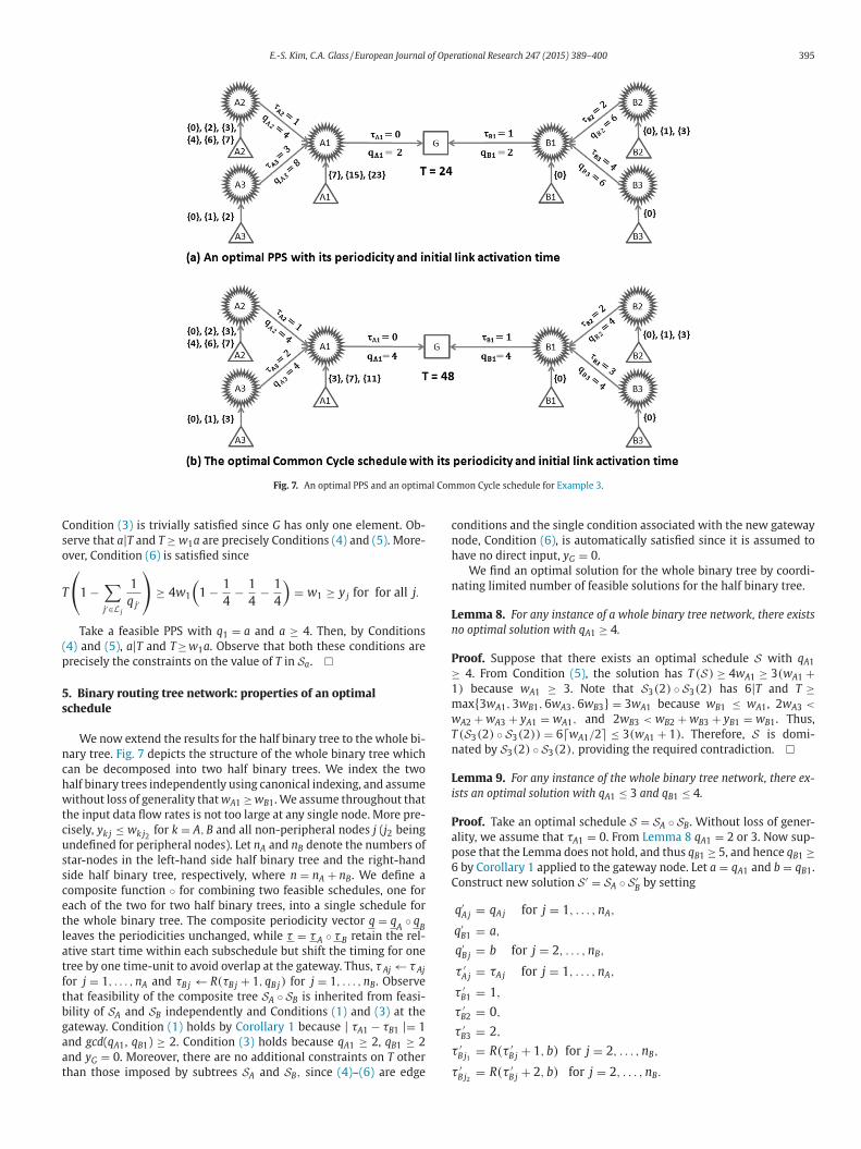
. Binary routing tree network: properties of an optimal

chedule

We now extend the results for the half binary tree to the whole bi-

ary tree. Fig. 7 depicts the structure of the whole binary tree which

an be decomposed into two half binary trees. We index the two

alf binary trees independently using canonical indexing, and assume

ithout loss of generality that wA1 ≥ wB1. We assume throughout that

he input data flow rates is not too large at any single node. More pre-

isely, yk j ≤ wk j2for k = A, B and all non-peripheral nodes j (j2 being

ndefined for peripheral nodes). Let nA and nB denote the numbers of

tar-nodes in the left-hand side half binary tree and the right-hand

ide half binary tree, respectively, where n = nA + nB. We define a

omposite function ◦ for combining two feasible schedules, one for

ach of the two for two half binary trees, into a single schedule for

he whole binary tree. The composite periodicity vector q = qA

◦ qB

eaves the periodicities unchanged, while τ = τ A ◦ τ B retain the rel-

tive start time within each subschedule but shift the timing for one

ree by one time-unit to avoid overlap at the gateway. Thus, τ Aj ← τ Aj

or j = 1, . . . , nA and τB j ← R(τB j + 1, qB j) for j = 1, . . . , nB. Observe

hat feasibility of the composite tree SA ◦ SB is inherited from feasi-

ility of SA and SB independently and Conditions (1) and (3) at the

ateway. Condition (1) holds by Corollary 1 because | τA1 − τB1 |= 1

nd gcd(qA1, qB1) ≥ 2. Condition (3) holds because qA1 ≥ 2, qB1 ≥ 2

nd yG = 0. Moreover, there are no additional constraints on T other

han those imposed by subtrees S and S , since (4)–(6) are edge

A B

onditions and the single condition associated with the new gateway

ode, Condition (6), is automatically satisfied since it is assumed to

ave no direct input, yG = 0.

We find an optimal solution for the whole binary tree by coordi-

ating limited number of feasible solutions for the half binary tree.

emma 8. For any instance of a whole binary tree network, there exists

o optimal solution with qA1 ≥ 4.

roof. Suppose that there exists an optimal schedule S with qA1

4. From Condition (5), the solution has T (S) ≥ 4wA1 ≥ 3(wA1 +) because wA1 ≥ 3. Note that S3(2) ◦ S3(2) has 6|T and T ≥ax{3wA1, 3wB1, 6wA3, 6wB3} = 3wA1 because wB1 ≤ wA1, 2wA3 <

A2 + wA3 + yA1 = wA1, and 2wB3 < wB2 + wB3 + yB1 = wB1. Thus,

(S3(2) ◦ S3(2)) = 6�wA1/2� ≤ 3(wA1 + 1). Therefore, S is domi-

ated by S3(2) ◦ S3(2), providing the required contradiction. �

emma 9. For any instance of the whole binary tree network, there ex-

sts an optimal solution with qA1 ≤ 3 and qB1 ≤ 4.

roof. Take an optimal schedule S = SA ◦ SB. Without loss of gener-

lity, we assume that τA1 = 0. From Lemma 8 qA1 = 2 or 3. Now sup-

ose that the Lemma does not hold, and thus qB1 ≥ 5, and hence qB1 ≥by Corollary 1 applied to the gateway node. Let a = qA1 and b = qB1.

onstruct new solution S ′ = SA ◦ S ′B by setting

q′A j = qA j for j = 1, . . . , nA,

q′B1 = a,

q′B j = b for j = 2, . . . , nB,

τ ′A j = τA j for j = 1, . . . , nA,

τ ′B1 = 1,

τ ′B2 = 0,

τ ′B3 = 2,

′B j1

= R(τ ′B j + 1, b) for j = 2, . . . , nB,

′B j = R(τ ′

B j + 2, b) for j = 2, . . . , nB.

2

396 E.-S. Kim, C.A. Glass / European Journal of Operational Research 247 (2015) 389–400

S

T

S

T

P

t

Sf

s

m

m

T

b

c

T

T

w

T

i

s

L

T

T

b

I

T

I

T

w

T

T

L

q

d

Observe that τ ′B j

, τ ′B j1

and τ ′B j2

satisfy Condition (1) by Lemma 1 for

j = 1, . . . nB. Condition (2) is satisfied because∑j′∈LB j

1

qj′= 1

qB j

+ 1

qB j1

+ 1

qB j2

≤ 1

a+ 1

b+ 1

b≤ 1

2+ 1

6+ 1

6= 5

6< 1 for j = 1, . . . , nB.

Condition (3) holds because q′A1

≥ 2, q′B1

≥ 2 and yG = 0. Thus, S ′ is

feasible. It remains to show that schedule S ′ is accommodated in

T (S), or equivalently that Conditions (4)–(6) are satisfied for the

given value of T (S). Condition (4) is satisfied because T (S) is divisible

by both qA1 = a and qB1 = b. Condition (5) is satisfied because

max{wA jq′A j, wB jq

′B j}

= max{wA1q′A1, max

j∈{2,...,nA}{wA jq

′A j}, wB1q′

B1, maxj∈{2,...,nB}

{wB jq′B j}}

= max{wA1a, maxj∈{2,...,nA}

{wA jq′A j}, wB1a, max

j∈{2,...,nB}{bwB j}}

≤ max{wA1a, maxj∈{2,...,nA}

{wA jqA j}, wB1b}= max{wA1qA1, max

j∈{2,...,nA}{wA jqA j}, wB1qB1}

≤ T (S).

Note that q′B1

≥ 2 and q′B j

≥ 6 for j = 2, . . . , nB. Moreover, since

T (S) ≥ q′B j

wB j = bwB j ≥ bwB j2≥ 6yB j for j = 1, . . . , nB,

T (S)

(1 −

∑j′∈LB j

1

qj′

)≥ 6yB j

(1 − 5

6

)≥ yB j,

and thus, Condition (6) is satisfied. �

From Lemmas 8 and 9, it is sufficient to consider only solutions

with qA1 = 2, 3 and qB1 = 2, 3, 4. Moreover, since qA1 and qB1 cannot

be co-prime from Corollary 1, when qA1 = 2 the value of qB1 is 2 or 4,

and when qA1 = 3 qB1 is 3. We now consider each of these three cases

in turn.

Lemma 10. Any feasible PPS for a whole binary tree with

qA1 = 3 is dominated by a solution S3(a) ◦ S3(a) with T =3a max {�wA1/a�, w} for some integer a ≥ 2, where w =max

{wk(2r+1) : r = 1, . . . , log2 nk and k = A, B

}.

Proof. Take a feasible schedule SA ◦ SB with qA1 = 3. As observed

above, qB1 = 3 from Corollary 1. Thus, by Lemma 6, SA and SB are

dominated by S3(aA) and S3(aB), respectively, where 3aA|T, 3aB|T,

T ≥ 3aA max {�wA1/aA�, wA} and T ≥ 3aB max {�wB1/aB�, wB} where

wA and wB are defined in Lemma 6. The rest of the proof follows by

setting a = aA if wA ≥ wB and a = aB if wA < wB, since wA1 ≥ wB1 and

w = max{wA, wB} as defined above. �

Lemma 11. Any feasible PPS for a whole binary tree with qA1 = qB1 =2 is dominated by one of the following solutions S2(2, a) ◦ S2(2, a) for

some integer a ≥ 2 with

T = 4a max

{⌈wA2

a

⌉, wA3,

⌈wB2

a

⌉, wB3

},

S2(2, 2) ◦ S2(3, 1) with

T = 24 max

{⌈wA2

6

⌉,

⌈wA3

3

⌉,

⌈wB2

4

⌉},

S2(2, a) ◦ S2(a, 1) and a ≥ 3 with

T = 4a max

{⌈wA2

a

⌉, wA3,

⌈wB2

2

⌉},

S2(3, 1) ◦ S2(2, 2) with

T = 24 max

{⌈wA2

4

⌉,

⌈wB2

6

⌉,

⌈wB3

3

⌉},

2(a, 1) ◦ S2(2, a) and a ≥ 3 with

= 4a max{⌈

wA2

2

⌉,

⌈wB2

a

⌉, wB3},

2(3, 1) ◦ S2(3, 1) with

= 6 max {wA2, wB2}.roof. From the result for a network containing a half binary sub-

ree in Lemma 5, it is sufficient to consider all combinations of

A = S2(2, a) for a ≥ 2 or SA = S2(a, 1) for a ≥ 3 and SB = S2(2, b)

or b ≥ 2 or SB = S2(b, 1) for b ≥ 3. We consider these cases

eparately.

Case 1: SA = S2(2, a) for a ≥ 2 and SB = S2(2, b) for b ≥ 2.

By Lemma 5, we have that 4a|T, 4b|T and T ≥ 4

ax {amax {�wA2/a�, wA3}, bmax {�wB2/b�, wB3}}. Thus, an opti-

al T value is of the form

≥ 4a′ max

{⌈wA2

a′

⌉, wA3,

⌈wB2

a′

⌉, wB3

},

y setting a′ = a if wA2 > wB2 and a′ = b if wA2 ≤ wB2.

Case 2: SA = S2(2, a) for a ≥ 2 and SB = S2(b, 1) for b ≥ 3.

We first consider the subcase when a = 2 and b = 3. In this sub-

ase, by Lemma 5, we have that 24|T and T ≥ max {4wA2, 8wA3, 6wB2}.

hus,

= 24 max

{⌈wA2

6

⌉,

⌈wA3

3

⌉,

⌈wB2

4

⌉}.

We now consider the subcase when a = 2 and b ≥ 4. By Lemma 5,

e have that 8|T, 2b|T and

≥ max{4wA2, 8wA3, 2bwB2}≥ max{4wA2, 8wA3, 4wB2, 8wB3}= 8 max

{⌈wA2

2

⌉, wA3,

⌈wB2

2

⌉, wB3

}= T (S2(2, 2) ◦ S2(2, 2)),

mplying that in this subcase, any solution can be dominated by a

olution S2(2, 2) ◦ S2(2, 2).

Finally, we consider the subcase when a ≥ 3 and b ≥ 3. Then, by

emma 5, we have that 4a|T, 2b|T and T ≥ max {4wA2, 4awA3, 2bwB2}.

hus, an optimal T value is of the form

= 4a′ max

{⌈wA2

a′

⌉, wA3,

⌈wB2

2

⌉},

y setting a′ = a if 4wA3 > 2wB3 and a′ = b if 4wA3 ≤ 2wB3.

Case 3: SA = S2(a, 1) for a ≥ 3 and SB = S2(2, b) for b ≥ 2

This case is similar to Case 2 but with the roles of a and b reversed.

f a = 3 and b = 2,

= 24 max

{⌈wA2

4

⌉,

⌈wA3

6

⌉,

⌈wB2

3

⌉}.

f a ≥ 3 and b ≥ 3, then

= 4a′ max

{⌈wA2

2

⌉,

⌈wB2

a′

⌉, wB3

},

here a′ = a if 2wA2 > 4wB3 and a′ = b if 2wA2 ≤ 4wB3.

Case 4: SA = S2(a, 1) for a ≥ 3 and SB = S2(b, 1) for b ≥ 3.

By Lemma 5, we have that 2a|T, 2b|T and

≥ max{2awA2, 2bwB2} ≥ 6 max{wA2, wB2}= T (S2(3, 1) ◦ S2(3, 1)).

hus, the solution is dominated by a solution S2(3, 1) ◦ S2(3, 1). �

emma 12. Any feasible PPS for a whole binary tree with qA1 = 2 and

B1 = 4, which is not dominated by a solution with qA1 = qB1 = 2, is

ominated by one of the following solutions

E.-S. Kim, C.A. Glass / European Journal of Operational Research 247 (2015) 389–400 397

T

T

P

b

t

S

4

T

i

3

T

m

T

N

t

s

o

a

6

c

S

t

w

t

a

i

s

L

f

S8

P

3

a

<

t

(

T ,

p

Ss

s

a

s

N

2

a

i

p

S

w

SS

S

S

a

S

S

T

t

P

t

L

f

f

w

w

a

a

T

g

T

S2(2, a) ◦ S4 for some integer a ≥ 3 with

= 4a max

{⌈wA2

a

⌉, wA3,

⌈wB1

a

⌉},

S2(3, 1) ◦ S4 with

= 12 max

{⌈wA2

2

⌉,

⌈wB1

3

⌉},

roof. Note that any feasible PPS SA ◦ SB with qB1 = 4 is dominated

y a solution with SB = S4 by Lemma 7. Since qA1 = 2, by Lemma 5

here are two cases to consider: SA = S2(2, a) for a ≥ 2, and SA =2(a, 1) for a ≥ 3.

Case 1: S2(2, a) ◦ S4 for a ≥ 2

By Lemmas 5 and 7, we have that 4a|T and T ≥ max {4wA2, 4awA3,

wB1}. If a = 2, then

= max{4wA2, 8wA3, 4wB1}= 8 max

{⌈wA2

2

⌉, wA3,

⌈wB1

2

⌉}≥ max

{⌈wA2

2

⌉, wA3,

⌈wB2

2

⌉, wB3

}= T (S2(2, 2) ◦ S2(2, 2)),

mplying that the solution is dominated by S2(2, 2) ◦ S2(2, 2). If a ≥, then

= 4a max

{⌈wA2

a

⌉, wA3,

⌈wB1

a

⌉}.

Case 2: S2(a, 1) ◦ S4 for a ≥ 3

By Lemmas 5 and 7, conditions on T are 4|T, 2a|T and T ≥ax {2awA2, 4wB1}. Thus, when a = 3,

= 12 max

{⌈wA2

2

⌉,

⌈wB1

3

⌉}.

ow take a ≥ 4 and compare S2(a, 1) ◦ S4 and its time frame T with

he alternative schedule S2(2, a) ◦ S4. The alternative schedule is fea-

ible with q′A2

= 4 < 2a = qA2, q′A j

= qA j = 2a or 4, for all other values

f j, and thus 4|T′, 2a|T′ and q′A j

≤ qA j for all values of j. Hence, T′ ≤ T

nd S2(a, 1) ◦ S4 is dominated by S2(2, a) ◦ S4. �

. Binary routing tree network: optimal algorithm

In the previous section we classified the forms which we need to

onsider for an optimal PPS for a binary tree in Lemmas 10 to 12.

everal of these forms are parameterised by the variable a and it is

herefore useful to reduce the range of potential values of a, which

e now do in the following Lemma. Algorithm OptPPS and Theorem 4

hen draws these results together. The efficiency of the optimisation

lgorithm OptPPS is considered at the end of the section, along with

ts effectiveness relative to the standard round robin, Common Cycle,

chedule.

emma 13. For a binary tree network, PPS of the following

orms S2(2, a) ◦ S2(a, 1), and S2(2, a) ◦ S2(2, a), S2(2, a) ◦ S4, and

2(a, 1) ◦ S2(2, a), may be optimal only for values of a less than 8, 8,

, and 5, respectively.

roof. Observe that we may restrict attention to the case T <

(wA1 + 1) since S3(2) ◦ S3(2) has T = 6�wA1/2� ≤ 3(wA1 + 1). In

ddition, it is sufficient to consider a solution with qA1 = 2 only if wA2

9wA3. To see this take an instance with wA2 ≥ 9wA3 and a PPS solu-

ion with qA1 = 2. Then, qA2 ≥ 4 by Lemma 4, and hence, by Condition

5) and the assumption that yA1 ≤ wA3,

≥ 4wA2 ≥ 3wA2 + 9wA3 ≥ 3wA2 + 3(wA3 + yA1 + 1) ≥ 3(wA1 + 1)

roviding the required contradiction.

Consider a solution with one of the following forms, S2(2, a) ◦2(a, 1), S2(2, a) ◦ S2(2, a) and S2(2, a) ◦ S4. In order for one of these

olutions to be optimal, it must hold that 4awA3 ≤ T < 3(wA1 + 1),

ince qA3 = 4a. Thus,

<3(wA1 + 1)

4wA3

= 3(wA2 + wA3 + yA1 + 1)

4wA3

≤ 3(wA2 + 3wA3)

4wA3

< 9,

ince we are restricting attention to instances for which wA2 < 9wA3.

ow consider a solution in the form of S2(a, 1) ◦ S2(2, a). It has qA2 =a and therefore 2awA2 < T ≤ 3(wA1 + 1). Hence,

<3(wA1 + 1)

2wA2

= 3(wA2 + wA3 + yA1 + 1)

2wA2

≤ 3(4wA2)

2wA2

≤ 6,

n an optimal solution. �

Algorithm OptPPS

Find the minimum T value amongst the following forms, and out-

ut in addition a corresponding schedule:

3(2) ◦ S3(2) with T = 6�wA1/2�;S3(a) ◦ S3(a) with T = 3wA1 for 3 ≤ a, a | wA1, and a < wA1/w

here w = max{

wk(2r+1) : r = 1, . . . , log2 nk and k = A, B}

;

2(2, 2) ◦ S2(2, 2) with T = 8 max{�wA2/2�, wA3, �wB2/2�, wB3};2(2, 2) ◦ S2(3, 1) with T = 24 max {�wA2/6�, �wA3/3�, �wB2/4�};

S2(2, a) ◦ S2(a, 1) with T = 4a max{�wA2/a�, wA3, �wB2/2�}for 3 ≤ a ≤ 8;

2(3, 1) ◦ S2(2, 2) with T = 24 max {�wA2/4�, �wB2/6�, �wB3/3�};S2(a, 1) ◦ S2(2, a) with T = 4a max{�wA2/2�, �wB2/a�, wB3}

for 3 ≤ a ≤ 5;2(3, 1) ◦ S2(3, 1) with T = 6 max {wA2, wB2};

S2(2, a) ◦ S2(2, a) with T = 4 max{wA2, wB2} for 3 ≤ a ≤ 8,

|max {wA2, wB2}, and a < max {wA2, wB2}/max {wA3, wB3};

2(2, a) ◦ S4withT = 4a max {�wA2/a�, wA3, �wB1/a�}for 3 ≤ a ≤ 8;

2(3, 1) ◦ S4withT = 12 max {�wA2/2�, �wB1/3�}.heorem 4. For a whole binary tree, Algorithm OptPPS provides an op-

imal perfect periodic schedule.

roof. We have established in the previous section that only solu-

ions with qA1 = qB1 = 3 and qA1 = 2 with qB1 = 2 or 4, described in

emmas 10, 11 and 12 need be considered.

When qA1 = qB1 = 3 potential optimal solutions are of the

orm S3(a) ◦ S3(a) with periodicity T = 3a max {�wA1/a�, w}rom Lemma 10. Now wA1 ≥ 2w, since wA1 ≥ wB1 and wk1 ≥

k2r−1 = wk2r+1 + wk2r + yk2r−1 > wk2r+1 + wk2r ≥ 2wk2r+1 because

k2r ≥ wk2r+1 from the indexing convention, for r = 1, . . . , log2 nknd k = A, B. Hence, �wA1/2� ≥ w and from the result in Appendix B

pplied to T/3, for a ≥ 2

={

3wA1 if there exists an integer a such thata | wA1 and 3 ≤ a < wA1/w,

6�wA1/2� otherwise,

iving rise to the first two forms.

The solution S2(2, a) ◦ S2(2, a) for a ≥ 2 has

=

⎧⎪⎨⎪⎩4 max{wA2, wB2} if there exists an integer

a such that a | max{wA2, wB2}and 3 ≤ a < max{wA2, wB2}/ max{wA3, wB3},

8 max{�wA2/2�, wA3, �wB2/2�, wB3} otherwise,

398 E.-S. Kim, C.A. Glass / European Journal of Operational Research 247 (2015) 389–400

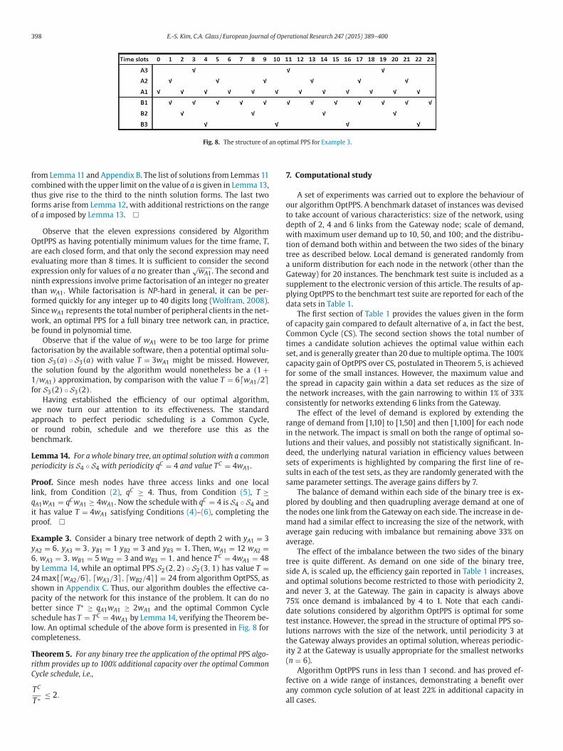
Fig. 8. The structure of an optimal PPS for Example 3.

7

o

t

d

w

t

t

a

G

s

p

d

o

C

t

s

c

f

t

t

c

r

i

l

d

s

s

s

p

t

m

a

a

t

s

a

a

7

d

t

l

t

i

(

f

a

a

from Lemma 11 and Appendix B. The list of solutions from Lemmas 11

combined with the upper limit on the value of a is given in Lemma 13,

thus give rise to the third to the ninth solution forms. The last two

forms arise from Lemma 12, with additional restrictions on the range

of a imposed by Lemma 13. �

Observe that the eleven expressions considered by Algorithm

OptPPS as having potentially minimum values for the time frame, T,

are each closed form, and that only the second expression may need

evaluating more than 8 times. It is sufficient to consider the second

expression only for values of a no greater than√

wA1. The second and

ninth expressions involve prime factorisation of an integer no greater

than wA1. While factorisation is NP-hard in general, it can be per-

formed quickly for any integer up to 40 digits long (Wolfram, 2008).

Since wA1 represents the total number of peripheral clients in the net-

work, an optimal PPS for a full binary tree network can, in practice,

be found in polynomial time.

Observe that if the value of wA1 were to be too large for prime

factorisation by the available software, then a potential optimal solu-

tion S3(a) ◦ S3(a) with value T = 3wA1 might be missed. However,

the solution found by the algorithm would nonetheless be a (1 +1/wA1) approximation, by comparison with the value T = 6�wA1/2�for S3(2) ◦ S3(2).

Having established the efficiency of our optimal algorithm,

we now turn our attention to its effectiveness. The standard

approach to perfect periodic scheduling is a Common Cycle,

or round robin, schedule and we therefore use this as the

benchmark.

Lemma 14. For a whole binary tree, an optimal solution with a common

periodicity is S4 ◦ S4 with periodicity qC = 4 and value TC = 4wA1.

Proof. Since mesh nodes have three access links and one local

link, from Condition (2), qC ≥ 4. Thus, from Condition (5), T ≥qA1wA1 = qCwA1 ≥ 4wA1. Now the schedule with qC = 4 is S4 ◦ S4 and

it has value T = 4wA1 satisfying Conditions (4)–(6), completing the

proof. �

Example 3. Consider a binary tree network of depth 2 with yA1 = 3

yA2 = 6, yA3 = 3, yB1 = 1 yB2 = 3 and yB3 = 1. Then, wA1 = 12 wA2 =6, wA3 = 3, wB1 = 5 wB2 = 3 and wB3 = 1, and hence TC = 4wA1 = 48

by Lemma 14, while an optimal PPS S2(2, 2) ◦ S2(3, 1) has value T =24 max{�wA2/6�, �wA3/3�, �wB2/4�} = 24 from algorithm OptPSS, as

shown in Appendix C. Thus, our algorithm doubles the effective ca-

pacity of the network for this instance of the problem. It can do no

better since T∗ ≥ qA1wA1 ≥ 2wA1 and the optimal Common Cycle

schedule has T = TC = 4wA1 by Lemma 14, verifying the Theorem be-

low. An optimal schedule of the above form is presented in Fig. 8 for

completeness.

Theorem 5. For any binary tree the application of the optimal PPS algo-

rithm provides up to 100% additional capacity over the optimal Common

Cycle schedule, i.e.,

TC

∗ ≤ 2.

T

. Computational study

A set of experiments was carried out to explore the behaviour of

ur algorithm OptPPS. A benchmark dataset of instances was devised

o take account of various characteristics: size of the network, using

epth of 2, 4 and 6 links from the Gateway node; scale of demand,

ith maximum user demand up to 10, 50, and 100; and the distribu-

ion of demand both within and between the two sides of the binary

ree as described below. Local demand is generated randomly from

uniform distribution for each node in the network (other than the

ateway) for 20 instances. The benchmark test suite is included as a

upplement to the electronic version of this article. The results of ap-

lying OptPPS to the benchmart test suite are reported for each of the

ata sets in Table 1.

The first section of Table 1 provides the values given in the form

f capacity gain compared to default alternative of a, in fact the best,

ommon Cycle (CS). The second section shows the total number of

imes a candidate solution achieves the optimal value within each

et, and is generally greater than 20 due to multiple optima. The 100%

apacity gain of OptPPS over CS, postulated in Theorem 5, is achieved

or some of the small instances. However, the maximum value and

he spread in capacity gain within a data set reduces as the size of

he network increases, with the gain narrowing to within 1% of 33%

onsistently for networks extending 6 links from the Gateway.

The effect of the level of demand is explored by extending the

ange of demand from [1,10] to [1,50] and then [1,100] for each node

n the network. The impact is small on both the range of optimal so-

utions and their values, and possibly not statistically significant. In-

eed, the underlying natural variation in efficiency values between

ets of experiments is highlighted by comparing the first line of re-

ults in each of the test sets, as they are randomly generated with the

ame parameter settings. The average gains differs by 7.

The balance of demand within each side of the binary tree is ex-

lored by doubling and then quadrupling average demand at one of

he nodes one link from the Gateway on each side. The increase in de-

and had a similar effect to increasing the size of the network, with

verage gain reducing with imbalance but remaining above 33% on

verage.

The effect of the imbalance between the two sides of the binary

ree is quite different. As demand on one side of the binary tree,

ide A, is scaled up, the efficiency gain reported in Table 1 increases,

nd optimal solutions become restricted to those with periodicity 2,

nd never 3, at the Gateway. The gain in capacity is always above

5% once demand is imbalanced by 4 to 1. Note that each candi-

ate solutions considered by algorithm OptPPS is optimal for some

est instance. However, the spread in the structure of optimal PPS so-

utions narrows with the size of the network, until periodicity 3 at

he Gateway always provides an optimal solution, whereas periodic-

ty 2 at the Gateway is usually appropriate for the smallest networks

n = 6).

Algorithm OptPPS runs in less than 1 second. and has proved ef-

ective on a wide range of instances, demonstrating a benefit over

ny common cycle solution of at least 22% in additional capacity in

ll cases.

E.-S. Kim, C.A. Glass / European Journal of Operational Research 247 (2015) 389–400 399

Ta

ble

1

Th

ere

sult

so

fth

ep

erf

orm

an

ceo

fO

ptP

PS

.

Test

sets

Pa

ram

ete

rse

ttin

gE

ffici

en

cyo

fN

um

be

ro

fti

me

sca

nd

ida

teso

luti

on

isid

en

tifi

ed

as

op

tim

al

by

Op

tPP

S

PP

So

ve

rC

S

Ch

ara

cte

rist

ico

f

inst

an

ceu

nd

er

inv

est

iga

tio

n

Va

ria

ble

sw

hic

hd

iffe

r

fro

md

efa

ult

va

lue

s1

Av

era

ge

(%)

Min

imu

m

(%)

Ma

xim

um

(%)

S 3(2

)◦

S 3(2

)

S 3(a

)◦

S 3(a

)

S 2(2

,2)◦

S 2(2

,2)

S 2(2

,2)◦

S 2(3

,1)

S 2(2

,a)◦

S 2(a

,1)

S 2(3

,1)◦

S 2(2

,2)

S 2(a

,1)◦

S 2(2

,a)

S 2(3

,1)◦

S 2(3

,1)

S 2(2

,a)◦

S 2(2

,a)

S 2(2

,a)◦

S 4S 2

(3,1)◦

S 4

Siz

eo

fn

etw

ork

(n=

6)

15

61

22

20

03

19

22

34

71

23

n=

30

13

91

31

15

26

08

40

21

50

02

n=

12

61

33

13

31

33

20

00

00

00

20

00

Sca

leo

fd

em

an

d(y

kj∼

U[1

,10

])1

61

12

51

90

10

14

41

24

60

13

yk

j∼

U[1

,50

]1

61

13

31

94

10

92

03

29

00

3

yk

j∼

U[1

,10

0]

15

41

31

19

54

19

52

23

51

13

Ba

lan

cein

de

ma

nd

on

en

od

efr

om

the

Ga

tew

ay

(yk

2∼

U[1

,10

])1

54

12

617

51

01

33

21

05

01

0

yk

2∼

U[2

0,3

0]

14

11

33

15

37

31

40

00

00

50

0

yk

2∼

U[4

0,5

0]

13

41

31

13

99

95

00

00

00

10

Ba

lan

cein

de

ma

nd

at

the

Ga

tew

ay

(yA

j∼

U[1

,10

])1

62

12

72

00

40

111

00

26

00

1

yA

j∼

U[2

0,3

0]

18

31

66

19

50

02

10

41

01

80

01

0

yA

j∼

U[4

0,5

0]

19

017

62

00

00

00

03

112

00

011

1D

efa

ult

pa

ram

ete

rv

alu

es

are

:n

=6,

yk

j∼

U[1

,10

]fo

rj=

1,..

.,n

kw

ith

k=

Ao

rB

.

8

N

p

i

l

n

l

w

w

G

t

s

u

s

r

t

g

T

o

t

f

t

p

o

c

a

l

s

a

n

t

d

c

t

t

s

t

a

i

n

t

i

o

o

A

E

e

q

A

m

P

S

2

w

b

. Conclusion

This paper examined packet scheduling in a Wireless Mesh access

etwork with a single Gateway to the Internet and identical link ca-

acities, and focus upon perfectly periodic schedules with the min-

mum time frame in which each peripheral client receives the same

evel of service. It focuses upon routing trees with a chain or a bi-

ary tree structure, producing optimal schedules for co-ordinating

ocal traffic generation with transmission across the access network

hich run in polynomial time. In doing so the research complements

ork on perfect periodic schedules at a single mesh node by Kim and

lass (2014), and on transmit schedules across the access network to

he Internet Gateway respecting pre-generated periodic local mesh

chedules (Allen et al., 2012).

The algorithms which we propose for a perfect periodic sched-

le along a chain, and through a binary tree network, form the ba-

is of a robust operating mechanism for WMNs. The chain algo-

ithm runs in polynomial time and is up to 50% more effective than

he optimal Common Cycle schedule. The binary tree scheduling al-

orithm effectively runs in polynomial time, of less than 1minute.

heoretically it is only demonstrably a PTAS relying on factorisation

f an integer. However, the integer under consideration represents

he number of clients in the network which is small enough to be

actorised quickly with current computer algorithms. The contribu-

ion of our algorithm is to provide up to double the throughput com-

ared to the optimal Common Cycle schedule for a binary tree. More-

ver, the nature of an optimal schedule makes it easy to convey to lo-

al nodes, and each solution remains optimal within a range of toler-

nce which depends only upon the relative cumulative transmission

oads through the links within two hops of the Gateway. Even out-

ide the tolerance range the solution will remain feasible with only

n incrementally increased time frame.

An important property revealed by this research is that for a bi-

ary routing tree in a uniform link capacity WMN, the minimum to-

al time frame of a PPS transmitting information to the Gateway is

etermined solely by the flow of data required through the six nodes

losest to the gateway. For a chain routing network it is the relative

raffic on the two links adjacent to the Gateway which determines

he form of an optimal solution for maximising the throughput. Ob-

erve that these properties may be used when assigning the routing

ree within the wireless access network, or indeed for designing the

ccess network itself. Thus, the simplicity and speed of our schedul-

ng algorithms ensure that they can be used to design the routing

etwork. The methodology developed in this paper provides analytic

ools for tackling more general routing trees. Future extensions might

nclude non-binary routing tree structures in WMNs, taking account

f secondary interference of two or more hops, and scheduling of

ther types of MANETs with similar equipment.

cknowledgments

This research was supported by EPSRC Grant number

P/G036454/1. The authors are grateful for the anonymous ref-

reeing process which resulted in a substantial improvement in the

uality of this article.

ppendix A

If a ≥ 2 and ab ≥ 3, then max{2w1, 2aw2, 2abw3} =ax{2aw2, 2abw3}.

roof. Consider the case when a = 2. Note that b ≥ 2 when a = 2.

uppose otherwise, then 4w2 = 2aw2 < 2w1 and 4bw3 = 2abw3 <

w1. From 4w2 < 2w1, we have that w2 < w1 − w2 = w2 + w3 + y1 −2 = w3 + y1. From 4bw3 < 2w1,

<w1

2w3

= w2 + w3 + y1

2w3

<2w3 + 2y1

2w3

= 1 + y1

w3

≤ 2,

400 E.-S. Kim, C.A. Glass / European Journal of Operational Research 247 (2015) 389–400

b

S

S

i

R

A

A

B

B

B

B

B

B

B

C

C

D

E

E

G

G

H

JK

L

M

P

P

Q

R

S

S

W

W

which contradicts to that b ≥ 2. Consider the case when a ≥ 3. Then,

2aw2 ≥ 6w2 = 2(w2 + w2 + w2) ≥ 2(w2 + w3 + y1) = 2w1. �

Appendix B

For given positive integers b and c such that b ≥ c, the set of values

T (a) = a max{�b/a�, c} for an integer a ≥ 2 has minimum value

T (a) = b if there exists a such that 3 ≤ a < b/c and a | b,

T (2) = 2 max{�b/2�, c} otherwise.

Proof. Consider the case when a = 2. If b < 2c, then T = 2c. If b ≥ 2c,

then

T (2) ={

b if b is an even number,b + 1 otherwise.

Consider the case when a ≥ 3. If b < ac, then

T (a) = ac ≥ max{2c, b + 1} ≥ T (2)

since a ≥ 3. If b ≥ ac, then

T (a) = a

⌈b

a

⌉≥

{b if a | b,

b + 1 otherwise.

Consequently,

mina≥3

T (a) ≥ T (2)

if there exists no integer a such that 3 ≤ a < b/c and a|b. �

Appendix C

Implementation of algorithm OptPPS on Example 3

In Example 3, wA1 = 12, wA2 = 6, wA3 = 3, wB1 = 5, wB2 = 3

and wB3 = 1. The condition on parameter values in OptPPS for

candidate schedules of the form S3(a) ◦ S3(a) restricts considera-

tion to a = 3 only, because 3 ≤ a < wA1/w and wA1 = 12 and w =max{wA3, wB3} = 3. Moreover, no schedule of the form S2(2, a) ◦S2(2, a) is a candidate because 3 ≤ a < max {wA2, wB2}/max {wA3,

wB3} and max{wA2, wB2}/ max{wA3, wB3} = 2, and hence algorithm

OptPPS evaluates T values for candidate list of schedules as follows:

S3(2) ◦ S3(2) : T = 6�wA1/2� = 36,

S3(2) ◦ S3(2) : T = 6�wA1/2� = 36,

S3(3) ◦ S3(3) : T = 3wA1 = 36,

S2(2, 2) ◦ S2(2, 2) : T = 8 max{�wA2/2�, wA3, �wB2/2�, wB3}= 24,

S2(2, 2) ◦ S2(3, 1) : T = 24 max {�wA2/6�, �wA3/3�, �wB2/4�}= 24,

S2(2, 3) ◦ S2(3, 1) : T = 12 max{�wA2/3�, wA3, �wB2/2�} = 36,

S2(2, 4) ◦ S2(4, 1) : T = 16 max{�wA2/4�, wA3, �wB2/2�} = 48,

S2(2, 5) ◦ S2(5, 1) : T = 20 max{�wA2/5�, wA3, �wB2/2�} = 60,

S2(2, 6) ◦ S2(6, 1) : T = 24 max{�wA2/6�, wA3, �wB2/2�} = 72,

S2(2, 7) ◦ S2(7, 1) : T = 28 max{�wA2/7�, wA3, �wB2/2�} = 84,

S2(2, 8) ◦ S2(8, 1) : T = 32 max{�wA2/8�, wA3, �wB2/2�} = 96,

S2(3, 1) ◦ S2(2, 2) : T = 24 max {�wA2/4�, �wB2/6�, �wB3/3�}= 48,

S2(3, 1) ◦ S2(2, 3) : T = 12 max{�wA2/2�, �wB2/3�, wB3} = 36,

S2(4, 1) ◦ S2(2, 4) : T = 16 max{�wA2/2�, �wB2/4�, wB3} = 48,

S2(5, 1) ◦ S2(2, 5) : T = 20 max{�wA2/2�, �wB2/5�, wB3} = 60,

S2(3, 1) ◦ S2(3, 1) : T = 6 max {wA2, wB2} = 36,

S2(2, 3) ◦ S4 : T = 12 max {�wA2/3�, wA3, �wB1/3�} = 36,

S2(2, 4) ◦ S4 : T = 16 max {�wA2/4�, wA3, �wB1/4�} = 48,

S2(2, 5) ◦ S4 : T = 20 max {�wA2/5�, wA3, �wB1/5�} = 60,

S2(2, 6) ◦ S4 : T = 24 max {�wA2/6�, wA3, �wB1/6�} = 72,

S2(2, 7) ◦ S4 : T = 28 max {�wA2/7�, wA3, �wB1/7�} = 84,

S2(2, 8) ◦ S4 : T = 32 max {�wA2/8�, wA3, �wB1/8�} = 96,

S2(3, 1) ◦ S4 : T = 12 max {�wA2/2�, �wB1/3�} = 36.

OptPPS picks up the minimum of these T values, 24, and outputs

oth schedules which achieve the T value of 24, namely S2(2, 2) ◦2(2, 2) and S2(2, 2) ◦ S2(3, 1), as optimal for Example 3.

upplementary material

Supplementary material associated with this article can be found,

n the online version, at 10.1016/j.ejor.2015.05.031

eferences

kyildiz, I. F., Wang, X., & Wang, W. (2005). Wireless mesh networks: a survey. Com-

puter Networks, 47, 445–487.

llen, S. M., Cooper, I. M., Glass, C. A., Kim, E.-S. Whitaker, R. M. (2012).Coordinating local schedules in wireless mesh networks. Working paper

(www.cs.cf.ac.uk/ISforWMN/Papers/CoordinatingWMN.pdf).ar-Noy, A., Bhatia, R., Naor, J., & Schieber, B. (2002a). Minimize service and operation

costs of periodic scheduling. Mathematics of Operations Research, 27, 518–544.ar-Noy, A., Dreizin, V., & Patt-Shamir, B. (2004). Efficient algorithms for periodic

scheduling. Computer Networks, 45, 155–173.

ar-Noy, A., Nisgav, A., & Patt-Shamir, B. (2002b). Nearly optimal perfectly periodicschedules. Distributed Computing, 15, 207–220.

jorklund, P., Varbrand, P., & Yuan, D. (2004). A column generation method for spatialtdma scheduling in ad hoc networks. Ad Hoc Networks, 2(4), 405–418.

rakerski, Z., Dreizin, V., & Patt-Shamir, B. (2003). Dispatching in perfectly-periodicschedules. Journal of Algorithm, 49, 219–239.

rakerski, Z., Nisgav, A., & Patt-Shamir, B. (2006). General perfectly periodic scheduling.Algorithmica, 45, 183–208.

rar, G., Blough, D., & Santi, P. (2006). Computationally efficient scheduling with the

physical interference model for throughput improvemen tin wireless mesh net-works. In Proceedings of ACM MobiCom 2006 (pp. 2–13).

hen, W.-M., & Huang, M.-K. (2008). Adaptive general perfectly periodic scheduling.In Proceedings of the international symposium on ubiquitous multimedia computing

(pp. 29–34).ommander, C. W., & Pardalos, P. M. (2009). A combinatorial algorithm for the tdma

message scheduling problem. Journal of Computational Optimization and Applica-

tions, 43(2), 449–463.as, A., Marks, R., Arabshahi, P., & Gray, A. (2005). Power controlled minimum frame

length scheduling in TDMA wireless networks with sectored antennas. In Proceed-ings IEEE INFOCOM 2005 (pp. 1782–1793).

lBatt, T., & Ephremides, A. (2004). Joint scheduling and power control for wirelessad-hoc networks. IEEE Transactions on Wireless Communications, 3, 74–85.

phremides, A., & Truong, T. (1990). Scheduling broadcasts in multihop radio networks.

IEEE Transactions on Communications, 38(4), 456–460.oussevskaia, O., Oswald, Y. A., & Wattenhofer, R. (2007). Complexity in geometric sinr.

In Proceedings of ACM MobiHoc 2007 (pp. 100–109).upta, A., Lin, X., & Srikant, R. (2007). Low-complexity distributed scheduling algo-

rithms for wireless networks. In Proceedings of IEEE INFOCOM 2007 (pp. 1631–1639).

ua, Q.-S., & Lau, F. C. (2008). Exact and approximate link scheduling algorithms under

the physical interference model. In Proceedings of ACM DIALM-POMC workshop 2008(pp. 45–54).

ones, G. A., & Jones, J. M. (1998). Elementrary Number Theory. Springer.im, E.-S., & Glass, C. A. (2014). Pefectly periodic scheduling for three basic cycles. Jour-

nal of Scheduling, 17(1), 47–65.i, Y., & Ephremides, A. (2007). A joint scheduling, powercontrol, and routing algorithm

for adhoc wireless networks. Ad Hoc Networks, 5(7), 959–973.

oscibroda, T., Wattenhofer, R., & Zollinger, A. (2006). Topology control meets sinr:the scheduling complexity of arbitrary topologies. In Proceedings of the 7th ACM

international symposium on mobile adhoc networking and computing (pp. 310–321).apadaki, K., & Friderikos, V. (2008). Approximate dynamic programming for link

scheduling in wireless mesh networks. Computers & Operations Research, 35(12),3848–3859.

atil, S., & Garg, V. K. (2006). Adaptive general perfectly periodic scheduling. Informa-tion Processing Letters, 98, 107–114.

uintas, D., & Friderikos, V. (2012). Energy efficient spatial tdma scheduling in wireless

networks. Computers & Operations Research, 39(9), 2091–2099.aman, B. (2006). Channel allocation in 802.11-based mesh networks. In Proceedings

of 25th IEEE international conference on computer communications Infocom 2006.(pp. 1–10).

arkar, S., & Ray, S. (2008). Arbitrary throughput versus complexity tradeoffs in wirelessnetworks using graph partitioning. IEEE Transactions on Automatic Control, 53(10),

2307–2323.

harma, G., Mazumdar, R. R., & Shroff, N. B. (2006). On the complexity of scheduling inwireless networks. In Proceedings of ACM MobiCom 2006 (pp. 227–238).

ang, G., & Ansari, N. (1997). Optimal broadcast scheduling in packet radio networksusing mean field annealing. IEEE Journal on Selected Areas in Communications, 15(2),

250–260.olfram, R. (2008). Mathematica 7.0. Wolfram Research, Champaign, Illinois, US.