Embed Size (px)
Citation preview

I/O scheduling strategy for periodic applications
ANA GAINARU, Vanderbilt University, USA
VALENTIN LE FÈVRE, École Normale Supérieure de Lyon, France
GUILLAUME PALLEZ (AUPY), Inria & University of Bordeaux, France
With the ever-growing need of data in HPC applications, the congestion at the I/O level becomes critical in
supercomputers. Architectural enhancement such as burst buffers and pre-fetching are added to machines,
but are not sufficient to prevent congestion. Recent online I/O scheduling strategies have been put in place,
but they add an additional congestion point and overheads in the computation of applications.
In this work, we show how to take advantage of the periodic nature of HPC applications in order to develop
efficient periodic scheduling strategies for their I/O transfers. Our strategy computes once during the job
scheduling phase a pattern which defines the I/O behavior for each application, after which the applications
run independently, performing their I/O at the specified times. Our strategy limits the amount of congestion
at the I/O node level and can be easily integrated into current job schedulers. We validate this model through
extensive simulations and experiments on an HPC cluster by comparing it to state-of-the-art online solutions,
showing that not only does our scheduler have the advantage of being de-centralized and thus overcoming
the overhead of online schedulers, but also that it performs better than the other solutions, improving the
application dilation up to 16% and the maximum system efficiency up to 18%.
Additional Key Words and Phrases: I/O, scheduling, periodicity, HPC, supercomputers
ACM Reference Format:Ana Gainaru, Valentin Le Fèvre, and Guillaume Pallez (Aupy). 2019. I/O scheduling strategy for periodic
applications. 1, 1 (May 2019), 25 pages. https://doi.org/10.1145/nnnnnnn.nnnnnnn
1 INTRODUCTION
Nowadays, supercomputing applications create or process TeraBytes of data. This is true in all
fields: for example LIGO (gravitational wave detection) generates 1500TB/year [30], the Large
Hadron Collider generates 15PB/year, light source projects deal with 300TB of data per day and
climate modeling are expected to have to deal with 100EB of data [22].
Management of I/O operations is critical at scale. However, observations on the Intrepid machine
at Argonne National Lab show that I/O transfer can be slowed down up to 70% due to conges-
tion [18]. For instance, when Los Alamos National Laboratory moved from Cielo to Trinity, the
peak performance moved from 1.4 Petaflops to 40 Petaflops (×28) while the I/O bandwidth moved
to 160 GB/s to 1.45TB/s (only ×9) [1]. The same kind of results can be observed at Argonne National
Laboratory when moving from Intrepid (0.6 PF, 88 GB/s) and to Mira (10PF, 240 GB/s). While
both peak performance and peak I/O improve, the reality is that I/O throughput scales worse
than linearly compared to performance, and hence, what should be noticed is a downgrade from
160 GB/PFlop (Intrepid) to 24 GB/PFlop (Mira).
Authors’ addresses: Ana Gainaru, Vanderbilt University, Nashville, TN, USA, [email protected]; Valentin Le Fèvre,
École Normale Supérieure de Lyon, France, [email protected]; Guillaume Pallez (Aupy), Inria & University of
Bordeaux, France, [email protected].
Permission to make digital or hard copies of all or part of this work for personal or classroom use is granted without fee
provided that copies are not made or distributed for profit or commercial advantage and that copies bear this notice and
the full citation on the first page. Copyrights for components of this work owned by others than ACM must be honored.
Abstracting with credit is permitted. To copy otherwise, or republish, to post on servers or to redistribute to lists, requires
prior specific permission and/or a fee. Request permissions from [email protected].
© 2019 Association for Computing Machinery.
XXXX-XXXX/2019/5-ART $15.00
https://doi.org/10.1145/nnnnnnn.nnnnnnn
, Vol. 1, No. 1, Article . Publication date: May 2019.

:2 Ana Gainaru, Valentin Le Fèvre, and Guillaume Pallez (Aupy)
With this in mind, to be able to scale, the conception of new algorithms has to change paradigm:
going from a compute-centric model to a data-centric model.
To help with the ever growing amount of data created, architectural improvements such as burst
buffers [2, 31] have been added to the system. Work is being done to transform the data before
sending it to the disks in the hope of reducing the I/O [14]. However, even with the current I/O
footprint burst buffers are not able to completely hide I/O congestion. Moreover, the data used is
always expected to grow. Recent works [18] have started working on novel online, centralized I/O
scheduling strategies at the I/O node level. However one of the risk noted on these strategies is the
scalability issue caused by potentially high overheads (between 1 and 5% depending on the number
of nodes used in the experiments) [18]. Moreover, it is expected that this overhead will increase at
larger scale since it need centralized information about all applications running in the system.
In this paper, we present a decentralized I/O scheduling strategy for supercomputers. We show
how to take known HPC application behaviors (namely their periodicity) into account to derive
novel static scheduling algorithms. This paper is an extended version of our previous work [4]. We
improve the main algorithm with a new loop aiming at correcting the size of the period at the end.
We also added a detailed complexity analysis and more simulations on synthetic applications to
show the wide applicability of our solution. Overall we consider that close to 50% of the technical
content is new material.
Periodic Applications. Many recent HPC studies have observed independent patterns in the I/O
behavior of HPC applications. The periodicity of HPC applications has been well observed and
documented [10, 15, 18, 25]: HPC applications alternate between computation and I/O transfer,
this pattern being repeated over-time. Carns et al. [10] observed with Darshan [10] the periodicity
of four different applications (MADBench2 [11], Chombo I/O benchmark [12], S3D IO [36] and
HOMME [35]). Furthermore, in our previous work [18] we were able to verify the periodicity of
gyrokinetic toroidal code (GTC) [16], Enzo [8], HACC application [20] and CM1 [7]. Furthermore,
fault-tolerance techniques (such as periodic checkpointing [13, 24]) also add to this periodic
behavior.
The key idea in this project is to take into account those known structural behaviors of HPC
applications and to include them in scheduling strategies.
Using this periodicity property, we compute a static periodic scheduling strategy (introduced
in our previous work [4]), which provides a way for each application to know when it should
start transferring its I/O (i) hence reducing potential bottlenecks due to I/O congestion, and (ii)
without having to consult with I/O nodes every time I/O should be done and hence adding an extra
overhead. The main contributions of this paper are:
• A novel light-weight I/O algorithm that looks at optimizing both application-oriented and
platform-oriented objectives;
• The full details of this algorithm and its implementation along with the full complexity
analysis;
• A set of extensive simulations and experiments that show that this algorithm performs as
well or better than current state of the art heavy-weight online algorithms.
• More simulations to show the performance at scale and a full evaluation to understand how
each parameter of the algorithm impacts its performance
Of course, not all applications exhibit a perfect periodic behavior, but based on our experience,
many of the HPC scientific applications have this property. This work is preliminary in the sense
that we are offering a proof of concept in this paper and we plan to tackle more complex patterns
in the future. In addition, future research will be done for including dynamic schedules instead of
only relying on static schedules. This work aims at being the basis of a new class of data-centric
, Vol. 1, No. 1, Article . Publication date: May 2019.

I/O scheduling strategy for periodic applications :3
scheduling algorithms based on well-know characteristics of HPC applications.
The algorithm presented here is done as a proof of concept to show the efficiency of these light-
weight techniques. We believe our scheduler can be implemented naturally into a data scheduler
(such as Clarisse [27]) and we provide experimental results backing this claim. We also give hints
of how this could be naturally coupled with non-periodic applications. However, this integration is
beyond the scope of this paper. For the purpose of this paper the applications are already scheduled
on the system and are able to receive information about their I/O scheduling. The goal of our I/O
scheduler is to eliminate congestion points caused by application interference while keeping the
overhead seen by all applications to the minimum. Computing a full I/O schedule over all iterations
of all applications is not realistic at today’s scale. The process would be too expensive both in time
and space. Our scheduler overcomes this by computing a period of I/O scheduling that includes
different number of iterations for each application.
The rest of the paper is organized as follows: in Section 2 we present the application model and
optimization problem. In Section 3 we present our novel algorithm technique as well as a brief
proof of concept for a future implementation. In Section 4 we present extensive simulations based
on the model to show the performance of our algorithm compared to state of the art. We then
confirm the performance by performing experiments on a supercomputer to validate the model.
We give some background and related work in Section 5. We provide concluding remarks and ideas
for future research directions in Section 6.
2 MODEL
In this section we use the model introduced in our previous work [18] that has been verified
experimentally to be consistent with the behavior of Intrepid and Mira, supercomputers at Argonne.
We consider scientific applications running at the same time on a parallel platform. The appli-
cations consist of series of computations followed by I/O operations. On a supercomputer, the
computations are done independently because each application uses its own nodes. However, the
applications are concurrently sending and receiving data during their I/O phase on a dedicated
I/O network. The consequence of this I/O concurrency is congestion between an I/O node of the
platform and the file storage.
2.1 Parameters
We assume that we have a parallel platform made up of N identical unit-speed nodes, composed of
the same number of identical processors, each equipped with an I/O card of bandwidth b (expressed
in bytes per second). We further assume having a centralized I/O system with a total bandwidth B(also expressed in bytes per second). This means that the total bandwidth between the computation
nodes and an I/O node is N · b while the bandwidth between an I/O node and the file storage is B,with usually N · b ≫ B. We have instantiated this model for the Intrepid platform on Figure 1.
We have K applications, all assigned to independent and dedicated computational resources, but
competing for I/O. For each application App(k )
we define:
• Its size: App(k )
executes with β (k ) dedicated processors;
• Its pattern: App(k )
obeys a pattern that repeats over time. There are n(k )tot
instances of App(k )
that are executed one after the other. Each instance consists of two disjoint phases: compu-
tations that take a time w (k ), followed by I/O transfers for a total volume vol(k)io. The next
instance cannot start before I/O operations for the current instance are terminated.
We further denote by rk the time when App(k )
is executed on the platform and dk the time when
the last instance is completed. Finally, we denote by γ (k )(t), the bandwidth used by a node on which
application App(k )
is running, at instant t . For simplicity we assume just one I/O transfer in each
, Vol. 1, No. 1, Article . Publication date: May 2019.

:4 Ana Gainaru, Valentin Le Fèvre, and Guillaume Pallez (Aupy)
b=0.1Gb/s/Node
=B
Fig. 1. Model instantiation for Intrepid [18].
App(1) w (1) w (1) w (1)
App(2) w (2) w (2) w (2)
App(3) w (3) w (3) w (3)
Bandwidth
Time0
0
B
Fig. 2. Scheduling the I/O of three periodic applications (top: computation, bottom: I/O).
loop. However, our model can be extended to work with multiple I/O patterns as long as these
are periodic in nature or as long as they are known in advance. In addition, our scheduler can
complement I/O prefetching mechanisms like [9, 23] that use the regular patterns within each data
access (contiguous/non-contiguous, read or write, parallel or sequential, etc) to avoid congestion.
2.2 Execution Model
As the computation resources are dedicated, we can always assume without loss of generality that
the next computation chunk starts immediately after completion of the previous I/O transfers, and
is executed at full (unit) speed. On the contrary, all applications compete for I/O, and congestion will
likely occur. The simplest case is that of a single periodic application App(k)
using the I/O system in
dedicated mode during a time-interval of duration D. In that case, let γ be the I/O bandwidth used
by each processor of App(k )
during that time-interval. We derive the condition β (k )γD = vol(k )io
to
express that the entire I/O data volume is transferred. We must also enforce the constraints that (i)
γ ≤ b (output capacity of each processor); and (ii) β (k )γ ≤ B (total capacity of I/O system). Therefore,
the minimum time to perform the I/O transfers for an instance of App(k )
is time(k )io=
vol(k )io
min(β (k )b ,B) .
However, in general many applications will use the I/O system simultaneously, and the bandwidth
capacity B will be shared among all applications (see Figure 2). Scheduling application I/O will
guarantee that the I/O network will not be loaded with more than its designed capacity. Figure 2
presents the view of the machine when 3 applications are sharing the I/O system. This translates at
the application level to delays inserted before I/O bursts (see Figure 3 for application 2’s point of
view).
This model is very flexible, and the only assumption is that at any instant, all processors assigned
to a given application are assigned the same bandwidth. This assumption is transparent for the I/O
, Vol. 1, No. 1, Article . Publication date: May 2019.
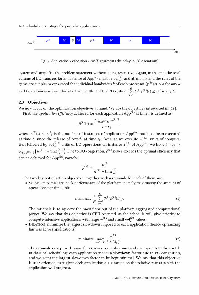
I/O scheduling strategy for periodic applications :5
App(2)
w (2) IO D IO w (2) IO w (2) IOBandwidth
Time
Fig. 3. Application 2 execution view (D represents the delay in I/O operations)
system and simplifies the problem statement without being restrictive. Again, in the end, the total
volume of I/O transfers for an instance of App(k )
must be vol(k )io, and at any instant, the rules of the
game are simple: never exceed the individual bandwidth b of each processor (γ (k )(t) ≤ b for any k
and t ), and never exceed the total bandwidth B of the I/O system (
K∑k=1
β (k )γ (k)(t) ≤ B for any t ).
2.3 Objectives
We now focus on the optimization objectives at hand. We use the objectives introduced in [18].
First, the application efficiency achieved for each application App(k )
at time t is defined as
ρ(k )(t) =
∑i≤n(k )(t )w
(k ,i)
t − rk,
where n(k )(t) ≤ n(k)tot
is the number of instances of application App(k )
that have been executed
at time t , since the release of App(k )
at time rk . Because we execute w (k ,i) units of computa-
tion followed by vol(k ,i)io
units of I/O operations on instance I(k )i of App
(k ), we have t − rk ≥∑
i≤n(k )(t )
(w (k ,i) + time
(k ,i)io
). Due to I/O congestion, ρ(k ) never exceeds the optimal efficiency that
can be achieved for App(k), namely
ρ(k ) =w (k )
w (k ) + time(k)io
The two key optimization objectives, together with a rationale for each of them, are:
• SysEff: maximize the peak performance of the platform, namely maximizing the amount of
operations per time unit:
maximize
1
N
K∑k=1
β (k )ρ(k )(dk ). (1)
The rationale is to squeeze the most flops out of the platform aggregated computational
power. We say that this objective is CPU-oriented, as the schedule will give priority to
compute-intensive applications with largew (k) and small vol(k )io
values.
• Dilation: minimize the largest slowdown imposed to each application (hence optimizing
fairness across applications):
minimize max
k=1..K
ρ(k )
ρ(k )(dk ). (2)
The rationale is to provide more fairness across applications and corresponds to the stretch
in classical scheduling: each application incurs a slowdown factor due to I/O congestion,
and we want the largest slowdown factor to be kept minimal. We say that this objective
is user-oriented, as it gives each application a guarantee on the relative rate at which the
application will progress.
, Vol. 1, No. 1, Article . Publication date: May 2019.

:6 Ana Gainaru, Valentin Le Fèvre, and Guillaume Pallez (Aupy)
We can now define the optimization problem:
Definition 1 (Periodic [18]). We consider a platform of N processors, a set of applications
∪Kk=1(App(k ), β (k ),w (k ), vol(k )
io), a maximum period Tmax, we want to find a periodic schedule P of
period T ≤ Tmax, in order to optimize one of the following objectives:
(1) SysEff
(2) Dilation
Note that it is known that both problems are NP-complete, even in an (easier) offline setting [18].
3 PERIODIC SCHEDULING STRATEGY
In general, for an application App(k ), n(k )
totthe number of instances of App
(k )is very large and
not polynomial in the size of the problem. For this reason, online schedules have been preferred
until now. The key novelty of this paper is to introduce periodic schedules for the K applications.
Intuitively, we are looking for a computation and I/O pattern of duration T that will be repeated
over time (except for initialization and clean up phases), as shown on Figure 4a. In this section, we
start by introducing the notion of periodic schedule and a way to compute the application efficiency
differently. We then provide the algorithms that are at the core of this work.
Because there is no competition on computation (no shared resources), we can consider that a
chunk of computation directly follows the end of the I/O transfer, hence we need only to represent
I/O transfers in this pattern. The bandwidth used by each application during the I/O operations is
represented over time, as shown in Figure 4b. We can see that an I/O operation can overlap with
the previous pattern or the next pattern, but overall, the pattern will just repeat.
Bw
Time
Init
· · ·
Pattern Clean up
c T+c 2T+c 3T+c (n−2)T+c (n−1)T+c nT+c
(a) Periodic schedule (phases)
Bw
Time0
0
T
B
vol(1)
iovol(1)
iovol(1)
io
vol(2)
io vol(2)
iovol(2)
io
vol(3)
iovol(3)
iovol(4)
io
initW(4)1
endW(4)1
initIO(4)1
(b) Detail of I/O in a period/pattern
Fig. 4. A schedule (above), and the detail of one of its regular pattern (below), where (w(1) = 3.5; vol(1)
io=
240;n(1)per= 3), (w(2) = 27.5; vol
(2)
io= 288;n
(2)per= 3), (w(3) = 90; vol
(3)
io= 350;n
(3)per= 1), (w(4) = 75; vol
(4)
io=
524;n(4)per= 1), and c is the duration of the initilization phase.
To describe a pattern, we use the following notations:
• n(k )per
: the number of instances of App(k)
during a pattern.
, Vol. 1, No. 1, Article . Publication date: May 2019.

I/O scheduling strategy for periodic applications :7
• I(k )i : the i-th instance of App
(k )during a pattern.
• initW(k )i : the time of the beginning of I(k )i . So, I
(k )i has a computation interval going from
initW(k )i to endW(k )i = initW(k )i +w(k )
mod T .
• initIO(k )i : the time when the I/O transfer from the i-th instance of App(k )
starts (between
endW(k)i and initIO(k )i , App(k )
is idle). Therefore, we have∫ initW(k )
(i+1)%n(k )per
initIO(k )i
β (k)γ (k )(t)dt = vol(k )io.
Globally, if we consider the two instants per instance initW(k )i and initIO(k )i , that define the change
between computation and I/O phases, we have a total of S ≤∑K
k=1 2n(k )per
distinct instants, that are
called the events of the pattern.
We define the periodic efficiency of a pattern of size T :
ρ(k )per=n(k )perw (k )
T. (3)
For periodic schedules, we use it to approximate the actual efficiency achieved for each application.
The rationale behind this can be seen in Figure 4. If App(k )
is released at time rk , and the first
pattern starts at time rk + c , that is after an initialization phase of duration c , then the main pattern
is repeated n times (until time n ·T + rk + c), and finally App(k )
ends its execution after a clean-up
phase of duration c ′ at time dk = rk +c+n ·T +c′. If we assume that n ·T ≫ c+c ′, then dk −rk ≈ n ·T .
Then the value of the ρ(k)(dk ) for App(k)
is:
ρ(k)(dk ) =
(n · n(k )
per+ δ
)w (k )
dk − rk=
(n · n(k )
per+ δ
)w (k )
c + n ·T + c ′
≈n(k )perw (k)
T= ρ(k )
per
where δ can be 1 or 0 depending whether App(k )
was executed or not during the clean-up or init
phase.
3.1 PerSched: a periodic scheduling algorithm
For details in the implementation, we refer the interested reader to the source code available at [17].
The difficulties of finding an efficient periodic schedule are three-fold:
• The right pattern size has to be determined;
• For a given pattern size, the number of instances of each application that should be included
in this pattern need to be determined;
• The time constraint between two consecutive I/O transfers of a given application, due to the
computation in-between makes naive scheduling strategies harder to implement.
Finding the right pattern size A solution is to find schedules with different pattern sizes between
a minimum pattern size Tmin and a maximum pattern size Tmax.
Because we want a pattern to have at least one instance of each application, we can trivially set
up Tmin = maxk (w(k ) + time
(k )io). Intuitively, the larger Tmax is, the more possibilities we can have
to find a good solution. However this also increases the complexity of the algorithm. We want to
limit the number of instances of all applications in a schedule. For this reason we chose to have
Tmax = O(maxk (w(k ) + time
(k )io)). We discuss this hypothesis in Section 4, where we give better
, Vol. 1, No. 1, Article . Publication date: May 2019.

:8 Ana Gainaru, Valentin Le Fèvre, and Guillaume Pallez (Aupy)
experimental intuition on finding the right value for Tmax. Experimentally we observe (Section 4,
Figure 11) that Tmax = 10Tmin seems to be sufficient.
We then decided on an iterative search where the pattern size increases exponentially at each
iteration from Tmin to Tmax. In particular, we use a precision ε as input and we iteratively increase
the pattern size from Tmin to Tmax by a factor (1 + ε). This allows us to have a polynomial number
of iterations. The rationale behind the exponential increase is that when the pattern size gets large,
we expect performance to converge to an optimal value, hence needing less the precision of a
precise pattern size. Furthermore while we could try only large pattern sizes, it seems important to
find a good small pattern size as it simplifies the scheduling step. Hence a more precise search for
smaller pattern sizes. Finally, we expect the best performance to cycle with the pattern size. We
verify these statements experimentally in Section 4 (Figure 10).
Determining the number of instances of each application By choosing Tmax = O(maxk (w(k ) +
time(k)io)), we guarantee the maximum number of instances of each application that fit into a pattern
is O
(maxk (w (k )+time
(k )io)
mink (w (k )+time(k )io)
).
Instance scheduling Finally, our last item is, given a pattern of size T , how to schedule instances
of applications into a periodic schedule.
To do this, we decided on a strategy where we insert instances of applications in a pattern, without
modifying dates and bandwidth of already scheduled instances. Formally, we call an application
schedulable:
Definition 2 (Schedulable). Given an existing pattern
P = ∪Kk=1
(n(k )per,∪
n(k )per
i=1 {initW(k )i , initIO
(k )i ,γ
(k )()}
), we say that an application App
(k )is schedulable
if there exists 1 ≤ i ≤ n(k )per
, such that:∫ initIO(k )i −w(k )
initW(k )i +w(k )
min
(β (k )b,B −
∑l
β (l )γ (l )(t)
)dt ≥ vol
(k )io
(4)
To understand Equation (4): we are checking that during the end of the computation of the
ith instance (initW(k )i +w(k)), and the beginning of the computation of the i + 1th instance to be,
there is enough bandwidth to perform at least a volume of I/O of vol(k )io. Indeed if a new instance is
inserted, initIO(k )i −w(k )
would then become the beginning of computation of the i + 1th instance.
Currently it is just some time before the I/O transfer of the ith instance. We represent it graphically
on Figure 5.
Bw
Time0
0
B
vol(1)
io 1vol(1)
io 2
vol(2)
io 1 vol(2)
io 2vol(2)
io 3
vol(3)
io
initW(2)2+w (2) initIO(2)
2−w (2)
Fig. 5. Graphical description of Definition 2: two instances of App(1)
and App(2)
are already scheduled. To
insert a third instance of App(2), we need to check that the blue area is greater than vol
(2)
iowith the bandwidth
constraint (because an instance of App(1)
is already scheduled, the bandwidth is reduced for the new instance
of App(2)). The red area is off limit for I/O (used for computations).
, Vol. 1, No. 1, Article . Publication date: May 2019.
I/O scheduling strategy for periodic applications :9
With Definition 2, we can now explain the core idea of the instance scheduling part of our
algorithm. Starting from an existing pattern, while there exist applications that are schedulable:
• Amongst the applications that are schedulable, we choose the application that has the worst
Dilation. The rationale is that even though we want to increase SysEff, we do it in a way
that ensures that all applications are treated fairly;
• We insert the instance into an existing scheduling using a procedure Insert-In-Pattern
such that (i) the first instance of each application is inserted using procedure Insert-First-
Instance which minimizes the time of the I/O transfer of this new instance, (ii) the other
instances are inserted just after the last inserted one.
Note that Insert-First-Instance is implemented using a water-filling algorithm [19] and Insert-
In-Pattern is implemented as described in Algorithm 1 below. We use a different function for
the first instance of each application because we do not have any previous instance to use the
Insert-In-Pattern function. Thus, the basic idea would be to put them at the beginning of the
pattern, but it will be more likely to create congestion if all applications are “synchronized” (for
example if all the applications are the same, they will all start their I/O phase at the same time). By
using Insert-First-Instance, every first instance will be at a place where the congestion for it is
minimized. This creates a starting point for the subsequent instances.
The function addInstance updates the pattern with the new instance, given a list of the intervals
(El , El ′,bl ) during which App(k )
transfers I/O between El and El ′ using a bandwidth bl .Correcting the period size In Algorithm 2, the pattern sizes evaluated are determined by Tmin
and ε . There is no reason why this would be the right pattern size, and one might be interested in
reducing it to fit precisely the instances that are included in the solutions that we found.
In order to do so, once a periodic pattern has been computed, we try to improve the best pattern
size we found in the first loop of the algorithm, by trying new pattern sizes, close to the previous
best one,Tcurr . To do this, we add a second loop which tries 1/ε uniformly distributed pattern sizes
from Tcurr to Tcurr /(1 + ε).With all of this in mind, we can now write PerSched (Algorithm 2), our algorithm to construct
a periodic pattern. For all pattern sizes tried between Tmin and Tmax, we return the pattern with
maximal SysEff.
3.2 Complexity analysis
In this section we show that our algorithm runs in reasonable execution time. We detail theoretical
results that allowed us to reduce the complexity. We want to show the following result:
Theorem 1. Let nmax =
(maxk (w (k )+time
(k )io)
mink (w (k )+time(k )io)
),
PerSched(K ′, ε, {App(k)}1≤k≤K ) runs in
O
((⌈1
ε
⌉+
⌈logK ′
log(1 + ε)
⌉)· K2 (nmax + logK
′)
).
Some of the complexity results are straightforward. The key results to show are:
• The complexity of the tests “while exists a schedulable application” on lines 11 and 23
• The complexity of computing A and finding its minimum element on line 13 and 25.
• The complexity of Insert-In-Pattern
To reduce the execution time, we proceed as follows: instead of implementing the set A, we
implement a heap A that could be summarized as
{App(k ) |App(k ) is not yet known to not be schedulable}
, Vol. 1, No. 1, Article . Publication date: May 2019.

:10 Ana Gainaru, Valentin Le Fèvre, and Guillaume Pallez (Aupy)
Algorithm 1: Insert-In-Pattern1 procedure Insert-In-Pattern(P, App(k ))
2 begin3 if App(k ) has 0 instance then4 return Insert-First-Instance (P,App(k ));
5 else6 Tmin := +∞ ;
7 Let I{i }k be the last inserted instance of App
(k );
8 Let E0, E1, · · · , Eji the times of the events between the end of I{i }k +w(k ) and the beginning
of I{(i+1) mod lT (k )}k ;
9 For l = 0 · · · ji − 1, let Bl be the minimum between β (k) b and the available bandwidth during
[El , El+1];
10 DataLeft = vol(k )io
;
11 l = 0;
12 sol = [];
13 while DataLeft > 0 and l < ji do14 if Bl > 0 then15 TimeAdded = min(El+1 − El ,DataLeft/Bl );
16 DataLeft -= TimeAdded·Bl ;
17 sol = [(El , El +TimeAdded,Bl )] + sol;
18 l++;
19 if DataLeft> 0 then20 return P21 else22 return P.addInstance(App(k),sol)
sorted following the lexicographic order:
(ρ (k )
ρ (k )per
, w (k )
time(k )io
). Hence, we replace the while loops on
lines 11 and 23 by the algorithm snippet described in Algorithm 3. The idea is to avoid calling
Insert-In-Pattern after each new inserted instance to know which applications are schedulable.
We then need to show that they are equivalent:
• At all time, the minimum element of A is minimal amongst the schedulable applications
with respect to the order
(ρ (k )
ρ (k )per
, w (k )
time(k )io
)(shown in Lemma 4);
• If A = ∅ then there are no more schedulable applications (shown in Corollary 2).
To show this, it is sufficient to show that (i) at all time,A ⊂ A, and (ii) A is always sorted according
to
(ρ (k )
ρ (k )per
, w (k )
time(k )io
).
Definition 3 (Compact pattern). We say that a patternP = ∪Kk=1
(n(k )per,∪
n(k )per
i=1 {initW(k )i , initIO
(k )i ,γ
(k )()}
)is compact if for all 1 ≤ i < n(k )
per, either initW(k )i +w
(k ) = initIO(k )i , or for all t ∈ [initW(k )i , initIO(k )i ],∑
l β(l )γ (l )(t) = B.
, Vol. 1, No. 1, Article . Publication date: May 2019.

I/O scheduling strategy for periodic applications :11
Algorithm 2: Periodic Scheduling heuristic: PerSched
1 procedure PerSched(K ′, ε, {App(k)}1≤k≤K )
2 begin3 Tmin ← maxk (w
(k ) + time(k )io);
4 Tmax ← K ′ ·Tmin;
5 T = Tmin;
6 SE← 0;
7 Topt ← 0;
8 Popt ← {};
9 while T ≤ Tmax do10 P = {};
11 while exists a schedulable application do12 A = {App(k ) |App(k ) is schedulable};
13 Let App(k )
be the element of A minimal with respect to the lexicographic order(ρ (k )
ρ (k )per
, w (k )
time(k )io
);
14 P←Insert-In-Pattern(P,App(k ));
15 if SE < SysEff(P) then16 SE← SysEff(P);
17 Topt ← T ;
18 Popt ← P
19 T ← T · (1 + ε);
20 T ← Topt;
21 while true do22 P = {};
23 while exists a schedulable application do24 A = {App(k ) |App(k ) is schedulable};
25 Let App(k )
be the element of A minimal with respect to the lexicographic order(ρ (k )
ρ (k )per
, w (k )
time(k )io
);
26 P←Insert-In-Pattern(P,App(k ));
27 if SysEff(P) = ToptT · SE then
28 Popt ← P;
29 T ← T − (Topt −Topt1+ε )/⌊1/ε⌋
30 else31 return Popt
We estimate SysEff of a periodic pattern, by replacing ρ (k )(dk ) by ρ(k )per
in Equation (1)
Intuitively, this means that, for all applications App(k), we can only schedule a new instance
between I(k )
n(k )per
and I(k )1
.
Lemma 1. At any time during PerSched, P is compact.
Proof. For each application, either we use Insert-First-Instance to insert the first instance
, Vol. 1, No. 1, Article . Publication date: May 2019.

:12 Ana Gainaru, Valentin Le Fèvre, and Guillaume Pallez (Aupy)
Algorithm 3: Schedulability snippet
11 A = ∪k {App(k )} (sorted by
(ρ (k )
ρ (k )per
, w (k )
time(k )io
));
12 while A , ∅ do13 Let App
(k )be the minimum element of A;
14 A ← A \ {App(k )};
15 Let P ′ =Insert-In-Pattern(P,App(k ));
16 if P ′ , P then17 P ← P ′;
18 Insert App(k )
in A following
(ρ (k )
ρ (k )per
, w (k )
time(k )io
);
(so P is compact as there is only one instance of an application at this step), or we use Insert-In-
Pattern which inserts an instance just after the last inserted one, which is the definition of being
compact. Hence, P is compact at any time during PerSched. □
Lemma 2. Insert-In-Pattern(P,App(k)) returns P, if and only if App(k )
is not schedulable.
Proof. One can easily check that Insert-In-Pattern checks the schedulability of App(k )
only
between the last inserted instance of App(k )
and the first instance of App(k ). Furthermore, because
of the compactness of P (Lemma 1), this is sufficient to test the overall schedulability.
Then the test is provided by the last condition Dataleft > 0.
• If the condition is false, then the algorithm actually inserts a new instance, so it means that
one more instance of App(k )
is schedulable.
• If the condition is true, it means that we cannot insert a new instance after the last inserted
one. Because P is compact, we cannot insert an instance at another place. So if the condition
is true, we cannot add one more instance of App(k )
in the pattern.
□
Corollary 1. In Algorithm 3, an application App(k)
is removed from A if and only if it is not
schedulable.
Lemma 3. If an application is not schedulable at some step, it will not be either in the future.
Proof. Let us suppose that App(k )
is not schedulable at some step. In the future, new instances of
other applications can be added, thus possibly increasing the total bandwidth used at each instant.
The total I/O load is non-decreasing during the execution of the algorithm. Thus if for all i , we had∫ initIO(k )i −w(k )
initW(k )i +w(k )
min
(β (k )b,B −
∑l
β (l )γ (l )(t)
)dt < vol
(k )io,
then in the future, with new bandwidths used γ ′(l )(t) > γ (l )(t), we will still have that for all i ,∫ initIO(k )i −w(k )
initW(k )i +w(k )
min
(β (k)b,B −
∑l
β (l )γ ′(l )(t)
)dt < vol
(k )io.
□
Corollary 2. At all time,
A = {App(k) |App(k ) is schedulable} ⊂ A.
, Vol. 1, No. 1, Article . Publication date: May 2019.

I/O scheduling strategy for periodic applications :13
This is a direct corollary of Corollary 1 and Lemma 3
Lemma 4. At all time, the minimum element of A is minimal amongst the schedulable applications
with respect to the order
(ρ (k )
ρ (k )per
, w (k )
time(k )io
)(but not necessarily schedulable).
Proof. First see that {App(k) |App(k ) is schedulable} ⊂ A. Furthermore, initially the minimality
property is true. Then the set A is modified only when a new instance of an application is added to
the pattern. More specifically, only the application that was modified has its position in A modified.
One can easily verify that for all other applications, their order with respect to
(ρ (k )
ρ (k )per
, w (k )
time(k )io
)has
not changed, hence the set is still sorted. □
This concludes the proof that the snippet is equivalent to the while loops. With all this we are
now able to show timing results for the version of Algorithm 2 that uses Algorithm 3.
Lemma 5. The loop on line 21 of Algorithm 2 terminates in at most ⌈1/ε⌉ steps.
Proof. The stopping criteria on line 27 checks that the number of instances did not change
when reducing the pattern size. Indeed, by definition for a pattern P,
SysEff(P) =∑k
β (k )ρ(k )per=
∑k β(k )n(k )
perw (k )
T.
Denote SE the SysEff reached in Topt at the end of the while loop on line 9 of Algorithm 2. Let
SysEff(P) be the SysEff obtained in Topt/(1 + ε). By definition,
SysEff(P) < SE and
Topt
1 + εSysEff(P) < ToptSE.
Necessarily, after at most ⌈1/ε⌉ iterations, Algorithm 2 exits the loop on line 21.
□
Proof of Theorem 1. There are ⌊m⌋ pattern sizes tried whereTmin · (1+ ε)m = Tmax in the main
“while” loop (line 9), that is
m =logTmax − logTmin
log(1 + ε)=
logK ′
log(1 + ε).
Furthermore, we have seen (Lemma 5) that there are a maximum of ⌈1/ε⌉ pattern sizes tried of the
second loop (line 21).
For each pattern size tried, the cost is dominated by the complexity of Algorithm 3. Let us
compute this complexity.
• The construction of A is done in O(K logK).• In sum, each application can be inserted a maximum of nmax times in A (maximum number of
instances in any pattern), that is the total of all insertions has a complexity ofO(K logKnmax).
We are now interested in the complexity of the different calls to Insert-In-Pattern.
First one can see that we only call Insert-First-Instance K times, and in particular they
correspond to the first K calls of Insert-In-Pattern. Indeed, we always choose to insert a new
instance of the application that has the largest current slowdown. The slowdown is infinite for
all applications at the beginning, until their first instance is inserted (or they are removed from
A) when it becomes finite, meaning that the K first insertions will be the first instance of all
applications.
, Vol. 1, No. 1, Article . Publication date: May 2019.

:14 Ana Gainaru, Valentin Le Fèvre, and Guillaume Pallez (Aupy)
During the k-th call, for 1 ≤ k ≤ K , there will be n = 2(k − 1) + 2 events (2 for each previously
inserted instances and the two bounds on the pattern), meaning that the complexity of Insert-First-
Instance will be O(n logn) (because of the sorting of the bandwidths available by non-increasing
order to choose the intervals to use). So overall, the K first calls have a complexity of O(K2logK).
Furthermore, to understand the complexity of the remaining calls to Insert-In-Pattern we are
going to look at the end result. In the end there is a maximum of nmax instance of each applications,
that is a maximum of 2nmaxK events. For all application App(k), for all instance I
(k )i k, 1 < i ≤ n(k ),
the only events considered in Insert-In-Pattern when scheduling I(k )i k were the ones between
the end of initW(i)k + w(k )
and initW(i)k+1. Indeed, since the schedule has been able to schedule
vol(k )io, Insert-In-Pattern will exit the while loop on line 13. Finally, one can see that the events
considered for all instances of an application partition the pattern without overlapping. Furthermore,
Insert-In-Pattern has a linear complexity in the number of events considered. Hence a total
complexity by application of O(nmaxK). Finally, we have K applications, the overall time spent in
Insert-In-Pattern for inserting new instances is O(K2nmax).
Hence, with the number of different pattern tried, we obtain a complexity of
O
((⌈m⌉ +
⌈1
ε
⌉) (K2
logK + K2nmax
) ).
□
In practice, both K ′ and K are small (≈ 10), and ε is close to 0, hence making the complexity
O( nmax
ε
).
3.3 High-level implementation, proof of concept
We envision the implementation of this periodic scheduler to take place at two levels:
1) The job schedulerwould know the applications profiles (using solutions such asOmnisc’IO [15]).
Using profiles it would be in charge of computing a periodic pattern every time an application
enters or leaves the system.
2) Application-side I/O management strategies (such as [27, 33, 41, 42]) then would be responsible
to ensure the correct I/O transfer at the right time by limiting the bandwidth used by nodes that
transfer I/O. The start and end time for each I/O as well as the used bandwidth are described in
input files.
To deal with the fact that some applications may not be fully-periodic, several directions could
be encompassed:
• Dedicating some part of the IO bandwidth to non-periodic applications depending on the
respective IO load of periodic and non-periodic applications;
• Coupling a dynamic I/O scheduler to the periodic scheduler;
• Using burst buffers to protect from the interference caused by non-predictable I/O.
Note that these directions are out of scope for this paper, as the goal of this paper aims to show a
proof-of-concept. Although future work will be devoted to the study of those directions.
4 EVALUATION AND MODEL VALIDATION
Note that the data used for this section and the scripts to generate the figures are available at https:
//github.com/vlefevre/ IO-scheduling-simu.
In this section, (i) we assess the efficiency of our algorithm by comparing it to a recent dynamic
framework [18], and (ii) we validate our model by comparing theoretical performance (as obtained
by the simulations) to actual performance on a real system.
, Vol. 1, No. 1, Article . Publication date: May 2019.
I/O scheduling strategy for periodic applications :15
We perform the evaluation in three steps: first we simulate behavior of applications and input
them into our model to estimate both Dilation and SysEff of our algorithm (Section 4.4) and
evaluate these cases on an actual machine to confirm the validity of our model. Finally, in Section 4.5
we confirm the intuitions introduced in Section 3 to determine the parameters used by PerSched.
4.1 Experimental Setup
The platform available for experimentation is Jupiter at Mellanox, Inc. To be able to verify our
model, we use it to instantiate our platformmodel. Jupiter is a Dell PowerEdge R720xd/R720 32-node
cluster using Intel Sandy Bridge CPUs. Each node has dual Intel Xeon 10-core CPUs running at 2.80
GHz, 25 MB of L3, 256 KB unified L2 and a separate L1 cache for data and instructions, each 32 KB
in size. The system has a total of 64GB DDR3 RDIMMs running at 1.6 GHz per node. Jupiter uses
Mellanox ConnectX-3 FDR 56Gb/s InfiniBand and Ethernet VPI adapters and Mellanox SwitchX
SX6036 36-Port 56Gb/s FDR VPI InfiniBand switches.
We measured the different bandwidths of the machine and obtained b = 0.01GB/s and B = 3GB/s.
Therefore, when 300 cores transfer at full speed (less than half of the 640 available cores), congestion
occurs.
Implementation of scheduler on Jupiter. We simulate the existence of such a scheduler by comput-
ing beforehand the I/O pattern for each application and providing it as an input file. The experiments
require a way to control for how long each application uses the CPU or stays idle waiting to start
its I/O in addition to the amount of I/O it is writing to the disk. For this purpose, we modified the
IOR benchmark [38] to read the input files that provide the start and end time for each I/O transfer
as well as the bandwidth used. Our scheduler generates one such file for each application. The
IOR benchmark is split in different sets of processes running independently on different nodes,
where each set represents a different application. One separate process acts as the scheduler and
receives I/O requests for all groups in IOR. Since we are interested in modeling the I/O delays due to
congestion or scheduler imposed delays, the modified IOR benchmarks do not use inter-processor
communications. Our modified version of the benchmark reads the I/O scheduling file and adapts
the bandwidth used for I/O transfers for each application as well as delaying the beginning of I/O
transfers accordingly.
We made experiments on our IOR benchmark and compared the results between periodic and
online schedulers as well as with the performance of the original IOR benchmark without any extra
scheduler.
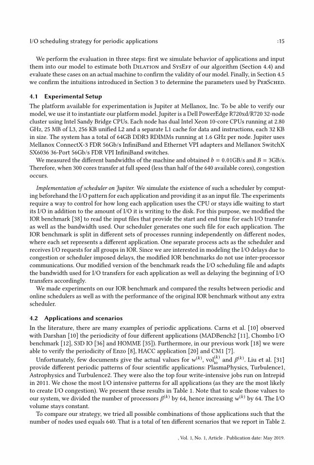
4.2 Applications and scenarios
In the literature, there are many examples of periodic applications. Carns et al. [10] observed
with Darshan [10] the periodicity of four different applications (MADBench2 [11], Chombo I/O
benchmark [12], S3D IO [36] and HOMME [35]). Furthermore, in our previous work [18] we were
able to verify the periodicity of Enzo [8], HACC application [20] and CM1 [7].
Unfortunately, few documents give the actual values for w (k), vol(k )io
and β (k ). Liu et al. [31]
provide different periodic patterns of four scientific applications: PlasmaPhysics, Turbulence1,
Astrophysics and Turbulence2. They were also the top four write-intensive jobs run on Intrepid
in 2011. We chose the most I/O intensive patterns for all applications (as they are the most likely
to create I/O congestion). We present these results in Table 1. Note that to scale those values to
our system, we divided the number of processors β (k ) by 64, hence increasingw (k ) by 64. The I/O
volume stays constant.
To compare our strategy, we tried all possible combinations of those applications such that the
number of nodes used equals 640. That is a total of ten different scenarios that we report in Table 2.
, Vol. 1, No. 1, Article . Publication date: May 2019.

:16 Ana Gainaru, Valentin Le Fèvre, and Guillaume Pallez (Aupy)
App(k ) w (k ) (s) vol
(k )io
(GB) β (k )
Turbulence1 (T1) 70 128.2 32,768
Turbulence2 (T2) 1.2 235.8 4,096
AstroPhysics (AP) 240 423.4 8,192
PlasmaPhysics (PP) 7554 34304 32,768
Table 1. Details of each application.
Set # T1 T2 AP PP
1 0 10 0 0
2 0 8 1 0
3 0 6 2 0
4 0 4 3 0
5 0 2 0 1
Set # T1 T2 AP PP
6 0 2 4 0
7 1 2 0 0
8 0 0 1 19 0 0 5 0
10 1 0 1 0
Table 2. Number of applications of each type
launched at the same time for each experiment
scenario.
Set # Application BW slowdown SysEff
1 Turbulence 2 65.72% 0.064561
2 Turbulence 2 63.93% 0.250105
AstroPhysics 38.12%
3 Turbulence 2 56.92% 0.439038
AstroPhysics 30.21%
4 Turbulence 2 34.9% 0.610826
AstroPhysics 24.92%
6 Turbulence 2 34.67% 0.621977
AstroPhysics 52.06%
10 Turbulence 1 11.79% 0.98547
AstroPhysics 21.08%
Table 3. Bandwidth slowdown, performance and application slowdown for each set of experiments
4.3 Baseline and evaluation of existing degradation
We ran all scenarios on Jupiter without any additional scheduler. In all tested scenarios congestion
occurred and decreased the visible bandwidth used by each applications as well as significantly
increased the total execution time. We present in Table 3 the average I/O bandwidth slowdown due
to congestion for the most representative scenarios together with the corresponding values for
SysEff. Depending on the I/O transfers per computation ratio of each application as well as how
the transfers of multiple applications overlap, the slowdown in the perceived bandwidth ranges
between 25% to 65%.
Interestingly, set 1 presents the worst degradation. This scenario is running concurrently ten
times the same application, which means that the I/O for all applications are executed almost at
the same time (depending on the small differences in CPU execution time between nodes). This
scenario could correspond to coordinated checkpoints for an application running on the entire
system. The degradation in the perceived bandwidth can be as high as 65% which considerably
increases the time to save a checkpoint. The use of I/O schedulers can decrease this cost, making
the entire process more efficient.
4.4 Comparison to online algorithms
In this subsection, we present the results obtained by running PerSched and the online heuristics
from our previous work [18]. Because in [18] we had different heuristics to optimize eitherDilation
or SysEff, in this work, the Dilation and SysEff presented are the best reached by any of those
heuristics. This means that there are no online solution able to reach them both at the same time!
, Vol. 1, No. 1, Article . Publication date: May 2019.
I/O scheduling strategy for periodic applications :17
We show that even in this scenario, our algorithm outperforms simultaneously these heuristics for
both optimization objectives!
The results presented in [18] represent the state of the art in what can be achieved with online
schedulers. Other solutions show comparable results, with [43] presenting similar algorithms but
focusing on dilation and [14] having the extra limitation of allowing the scheduling of only two
applications.
PerSched takes as input a list of applications, as well as the parameters, presented in Section 3,
K ′ = Tmax
Tmin
, ε . All scenarios were tested with K ′ = 10 and ε = 0.01.
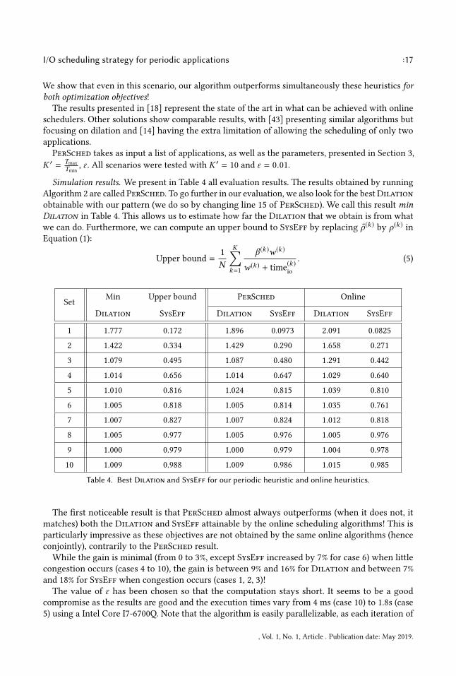
Simulation results. We present in Table 4 all evaluation results. The results obtained by running
Algorithm 2 are called PerSched. To go further in our evaluation, we also look for the bestDilation
obtainable with our pattern (we do so by changing line 15 of PerSched). We call this result min
Dilation in Table 4. This allows us to estimate how far the Dilation that we obtain is from what
we can do. Furthermore, we can compute an upper bound to SysEff by replacing ρ(k ) by ρ(k ) inEquation (1):
Upper bound =1
N
K∑k=1
β (k )w (k )
w (k ) + time(k)io
. (5)
Set
Min Upper bound PerSched Online
Dilation SysEff Dilation SysEff Dilation SysEff
1 1.777 0.172 1.896 0.0973 2.091 0.0825
2 1.422 0.334 1.429 0.290 1.658 0.271
3 1.079 0.495 1.087 0.480 1.291 0.442
4 1.014 0.656 1.014 0.647 1.029 0.640
5 1.010 0.816 1.024 0.815 1.039 0.810
6 1.005 0.818 1.005 0.814 1.035 0.761
7 1.007 0.827 1.007 0.824 1.012 0.818
8 1.005 0.977 1.005 0.976 1.005 0.976
9 1.000 0.979 1.000 0.979 1.004 0.978
10 1.009 0.988 1.009 0.986 1.015 0.985
Table 4. Best Dilation and SysEff for our periodic heuristic and online heuristics.
The first noticeable result is that PerSched almost always outperforms (when it does not, it
matches) both the Dilation and SysEff attainable by the online scheduling algorithms! This is
particularly impressive as these objectives are not obtained by the same online algorithms (hence
conjointly), contrarily to the PerSched result.
While the gain is minimal (from 0 to 3%, except SysEff increased by 7% for case 6) when little
congestion occurs (cases 4 to 10), the gain is between 9% and 16% for Dilation and between 7%
and 18% for SysEff when congestion occurs (cases 1, 2, 3)!
The value of ε has been chosen so that the computation stays short. It seems to be a good
compromise as the results are good and the execution times vary from 4 ms (case 10) to 1.8s (case
5) using a Intel Core I7-6700Q. Note that the algorithm is easily parallelizable, as each iteration of
, Vol. 1, No. 1, Article . Publication date: May 2019.

:18 Ana Gainaru, Valentin Le Fèvre, and Guillaume Pallez (Aupy)
0.4
0.6
0.8
1.0
1 2 3 4 5 6 7 8 9 10Set
Syst
em E
ffici
ency
/ U
pper
bou
nd
Periodic (expe)Periodic (simu)Online (expe)Online (simu)Congestion
(a) SysEff/ Upper bound SysEff
1.2
1.5
1.8
2.1
1 2 3 4 5 6 7 8 9 10Set
Dila
tion
Periodic (expe)Periodic (simu)Online (expe)Online (simu)
(b) Dilation
Fig. 6. Performance for both experimental evaluation and theoretical (simulated) results. The performance
estimated by our model is accurate within 3.8% for periodic schedules and 2.3% for online schedules.
Platform B (GB/s) b (GB/s) N N ·bB GFlops/node
Intrepid 64 0.0125 40,960 8 2.87
Mira 240 0.03125 49,152 6 11.18
Table 5. Bandwidth and number of processors of each platform used for simulations.
the loop is independent. Thus it may be worth considering a smaller value of ε , but we expect nobig improvement on the results.
Model validation through experimental evaluation. We used the modified IOR benchmark to
reproduce the behavior of applications running on HPC systems and analyze the benefits of I/O
schedulers. We made experiments on the 640 cores of the Jupiter system. Additionally to the
results from both periodic and online heuristics, we present the performance of the system with no
additional I/O scheduler.
Figure 6 shows the SysEff (normalized using the upper bound in Table 4) and Dilation when
using the periodic scheduler in comparison with the online scheduler. The results when applications
are running without any scheduler are also shown. As observed in the previous section, the periodic
scheduler gives better or similar results to the best solutions that can be returned by the online
ones, in some cases increasing the system performance by 18% and the dilation by 13%. When we
compare to the current strategy on Jupiter, the SysEff reach 48%! In addition, the periodic scheduler
has the benefit of not requiring a global view of the execution of the applications at every moment
of time (by opposition to the online scheduler).
Finally, a key information from those results is the precision of our model introduced in Section 2.
The theoretical results (based on the model) are within 3% of the experimental results!
This observation is key in launching more thorough evaluation via extensive simulations and is
critical in the experimentation of novel periodic scheduling strategies.
Synthetic applications. The previous experiments showed that our model can be used to simulate
real life machines (that was already observed for Intrepid and Mira in [18]). In this next step, we
now rely on synthetic applications and simulation to test extensively the efficiency of our solution.
We considered two platforms (Intrepid and Mira) to run the simulations with concrete values of
bandwidths (B,b) and number of nodes (N ). The values are reported in Table 5.
, Vol. 1, No. 1, Article . Publication date: May 2019.

I/O scheduling strategy for periodic applications :19
The parameters of the synthetic applications are generated as followed:
• w (k ) is chosen uniformly at random between 2 and 7500 seconds for Intrepid (and between
0.5 and 1875s for Mira whose nodes are about 4 times faster than Intrepid’s nodes),
• the volume of I/O data vol(k )io
is chosen uniformly at random between 100 GB and 35 TB.
These values where based on the applications we previously studied.
We generate the different sets of applications using the following method: let n be the number of
unused nodes. At the beginning we set n = N .
(1) Draw uniformly at random an integer number x between 1 and max(1, n4096− 1) (to ensure
there are at least two applications).
(2) Add to the set an application App(k)
with parametersw (k ) and vol(k )io
set as previously detailed
and β (k) = 4096x .(3) n ← n − 4096x .(4) Go to step 1 if n > 0.
We then generated 100 sets for Intrepid (using a total of 40,960 nodes) and 100 sets for Mira (using
a total of 49,152 nodes) on which we run the online algorithms (either maximizing the system
efficiency or minimizing the dilation) and PerSched. The results are presented on Figures 7a and 7b
for simulations using the Intrepid settings and Figures 8a and 8b for simulations using the Mira
settings.
0.6
0.8
1.0
0 25 50 75 100Set
Syst
em E
ffici
ency
/ U
pper
bou
nd
PeriodicOnline (best)
(a) SysEff/ Upper bound SysEff
1.0
1.2
1.4
1.6
0 25 50 75 100Set
Dila
tion
PeriodicOnline (best)
(b) Dilation
Fig. 7. Comparison between online heuristics and PerSched on synthetic applications, based on Intrepid
settings.
We can see that overall, our algorithm increases the system efficiency in almost every case. On
average the system efficiency is improved by 16% on intrepid (32% on Mira) with peaks up to 116%!
On Intrepid the dilation has overall similar values (an average of 0.6% degradation over the best
online algorithm, with variation between 11% improvement and 42% degradation). However on
Mira in addition to the improvement in system efficiency, PerSched improves on average by 22%
the dilation!
The main difference between Intrepid and Mira is the ratio compute (= N · GFlops/node) overI/O bandwidth (B). In other terms, that is the speed at which data is created/used over the speed
at which data is transferred. Note that as said earlier, the trend is going towards an increase of
this ratio. This ratio increases a lot (and hence incurring more I/O congestion) on Mira. To see if
this indeed impacts the performance of our algorithm, we plot on Figure 9 the average results of
running 100 synthetic scenarios on systems with different ratios of compute over I/O. Basically,
, Vol. 1, No. 1, Article . Publication date: May 2019.

:20 Ana Gainaru, Valentin Le Fèvre, and Guillaume Pallez (Aupy)
0.4
0.6
0.8
1.0
0 25 50 75 100Set
Syst
em E
ffici
ency
/ U
pper
bou
nd
PeriodicOnline (best)
(a) SysEff/ Upper bound SysEff
1
2
3
0 25 50 75 100Set
Dila
tion
PeriodicOnline (best)
(b) Dilation
Fig. 8. Comparison between online heuristics and PerSched on synthetic applications, based on Mira settings.
the systems we simulate have identical performance to Mira (Table 5), and we only increase the
GFlops/node by a ratio from 2 to 1024. We plot the SysEff improvement factor (SysEff(Online)
SysEff(PerSched))
and the Dilation improvement factor (Dilation(Online)
Dilation(PerSched)).
Fig. 9. Comparison between online heuristics and PerSched on synthetic applications, for different ratios of
compute over I/O bandwidth.
The trend that can be observed is that PerSched seems to be a lot more efficient on systems
where congestion is even more critical, showing that this algorithm seems to be even more useful at
scale. Specifically, when the ratio increases from 2 to 1024 the gain in SysEff increases on average
from 1.1 to 1.5, and at the same time, the gain in Dilation increases from 1.2 to 1.8.
4.5 Discussion on finding the best pattern size
The core of our algorithm is a search of the best pattern size via an exponential growth of the
pattern size until Tmax. As stated in Section 3, the intuition of the exponential growth is that the
larger the pattern size, the less precision is needed for the pattern size as it might be easier to fit
many instances of each application. On the contrary, we expect that for small pattern sizes finding
the right one might be a precision job.
, Vol. 1, No. 1, Article . Publication date: May 2019.

I/O scheduling strategy for periodic applications :21
0.080
0.085
0.090
0.095
2500 5000 7500
SysE
ff
Set 1
2.0
2.5
3.0
3.5
2500 5000 7500
Dila
tion
0.175
0.200
0.225
0.250
0.275
40000 80000 120000 160000
Set 2
1.50
1.75
2.00
2.25
40000 80000 120000 160000
0.30
0.35
0.40
0.45
40000 80000 120000 160000
Set 3
1.25
1.50
1.75
2.00
40000 80000 120000 160000
0.350.400.450.500.550.600.65
40000 80000 120000 160000
Set 4
1.00
1.25
1.50
1.75
2.00
40000 80000 120000 160000
0.5
0.6
0.7
0.8
1e+06 2e+06 3e+06 4e+06 5e+06
Set 5
1.00
1.25
1.50
1.75
2.00
1e+06 2e+06 3e+06 4e+06 5e+06
0.5
0.6
0.7
0.8
40000 80000 120000 160000
SysE
ff
Set 6
1.00
1.25
1.50
1.75
2.00
40000 80000 120000 160000Period
Dila
tion
0.5
0.6
0.7
0.8
10000 20000 30000 40000
Set 7
1.00
1.25
1.50
1.75
2.00
10000 20000 30000 40000Period
0.6
0.7
0.8
0.9
1e+06 2e+06 3e+06 4e+06 5e+06
Set 8
1.00
1.25
1.50
1.75
2.00
1e+06 2e+06 3e+06 4e+06 5e+06Period
0.5
0.6
0.7
0.8
0.9
1.0
40000 80000 120000 160000
Set 9
1.00
1.25
1.50
1.75
2.00
40000 80000 120000 160000Period
0.80
0.85
0.90
0.95
40000 80000 120000 160000
Set 10
1.00
1.25
1.50
1.75
2.00
40000 80000 120000 160000Period
Fig. 10. Evolution of SysEff (blue) and Dilation (pink) when the pattern size increases for all sets.
Set ninst nmax
1 11 1.00
2 25 35.2
3 33 35.2
4 247 35.2
5 1086 1110
Set ninst nmax
6 353 35.2
7 81 10.2
8 251 31.5
9 9 1.00
10 28 3.47
Table 6. Maximum number of instances per application (ninst) in the solution returned by PerSched, ratio
between longest and shortest application (nmax).
We verify this experimentally and plot on Figure 10 the SysEff and Dilation found by our
algorithm as a function of the pattern size T for all the 10 sets. We can see that they all have very
similar shape.
Finally, the last information to determine to tweak PerSched is the value of Tmax. Remember
that we denote K ′ = Tmax/Tmin.
To be able to get an estimate of the pattern size returned by PerSched, we provide in Table 6 (i)
the maximum number of instances ninst of any application, and (ii) the ratio nmax =maxk
(w (k )+time
(k )io
)mink
(w (k )+time
(k )io
) .Together along with the fact that the Dilation (Table 4) is always below 2 they give a rough idea
of K ′ (≈ ninst
nmax
). It is sometimes close to 1, meaning that a small value of K ′ can be sufficient, but
choosing K ′ ≈ 10 is necessary in the general case.
We then want to verify the cost of under-estimating Tmax. For this evaluation all runs were done
up to K ′ = 100 with ε = 0.01. Denote SysEff(K ′) (resp. Dilation(K ′)) the maximum SysEff (resp.
corresponding Dilation) obtained when running PerSched with K ′. We plot their normalized
version that is:
SysEff(K ′)
SysEff(100)
(resp.
Dilation(K ′)
Dilation(100)
)on Figure 11. The main noticeable information is that the convergence is very fast: when K ′ = 3,
, Vol. 1, No. 1, Article . Publication date: May 2019.
:22 Ana Gainaru, Valentin Le Fèvre, and Guillaume Pallez (Aupy)
0.97
0.98
0.99
1.00
1 2 3 4 5 6 7 8 9 10 11 12 13 14 15K' = Tmax / Tmin
Nor
mal
ized
Sys
Eff
1.00
1.05
1.10
1.15
1 2 3 4 5 6 7 8 9 10 11 12 13 14 15K' = Tmax / Tmin
Nor
mal
ized
Dila
tion
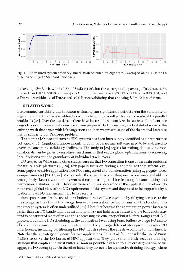
Fig. 11. Normalized system efficiency and dilation obtained by Algorithm 2 averaged on all 10 sets as a
function of K ′ (with Standard Error bars).
the average SysEff is within 0.3% of SysEff(100), but the corresponding average Dilation is 5%
higher than Dilation(100). If we go to K ′ = 10 then we have a SysEff of 0.1% of SysEff(100) and
a Dilation within 1% of Dilation(100)! Hence validating that choosing K ′ = 10 is sufficient.
5 RELATEDWORK
Performance variability due to resource sharing can significantly detract from the suitability of
a given architecture for a workload as well as from the overall performance realized by parallel
workloads [39]. Over the last decade there have been studies to analyze the sources of performance
degradation and several solutions have been proposed. In this section, we first detail some of the
existing work that copes with I/O congestion and then we present some of the theoretical literature
that is similar to our Periodic problem.
The storage I/O stack of current HPC systems has been increasingly identified as a performance
bottleneck [32]. Significant improvements in both hardware and software need to be addressed to
overcome oncoming scalability challenges. The study in [26] argues for making data staging coor-
dination driven by generic cross-layer mechanisms that enable global optimizations by enforcing
local decisions at node granularity at individual stack layers.
I/O congestionWhile many other studies suggest that I/O congestion is one of the main problems
for future scale platforms [6, 34], few papers focus on finding a solution at the platform level.
Some papers consider application-side I/O management and transformation (using aggregate nodes,
compression etc) [33, 41, 42]. We consider those work to be orthogonal to our work and able to
work jointly. Recently, numerous works focus on using machine learning for auto tuning and
performance studies [5, 29]. However these solutions also work at the application level and do
not have a global view of the I/O requirements of the system and they need to be supported by a
platform level I/O management for better results.
Some paper consider the use of burst buffers to reduce I/O congestion by delaying accesses to the
file storage, as they found that congestion occurs on a short period of time and the bandwidth to
the storage system is often underutilized [31]. Note that because the computation power increases
faster than the I/O bandwidth, this assumption may not hold in the future and the bandwidth may
tend to be saturated more often and thus decreasing the efficiency of burst buffers. Kougas et al. [28]
present a dynamic I/O scheduling at the application level using burst buffers to stage I/O and to
allow computations to continue uninterrupted. They design different strategies to mitigate I/O
interference, including partitioning the PFS, which reduces the effective bandwidth non-linearly.
Note that their strategy only consider two applications. Tang et al. [40] consider the use of Burst-
Buffers to serve the I/O bursts of HPC applications. They prove that a basic reactive draining
strategy that empties the burst buffer as soon as possible can lead to a severe degradation of the
aggregate I/O throughput. On the other hand, they advocate for a proactive draining strategy, where
, Vol. 1, No. 1, Article . Publication date: May 2019.

I/O scheduling strategy for periodic applications :23
data is divided into draining segments which are dispersed evenly over the I/O interval, and the
burst buffer draining throughput is controlled through adjusting the number of I/O requests issued
each time. Recently, Aupy et al. [3] have started discussing coupling of IO scheduling and buffers
partitionning to improve data scheduling. They propose an optimal algorithm that determines the
minimum buffer size needed to avoid congestion altogether.
The study from [37] offers ways of isolating the performance experienced by applications of one
operating system from variations in the I/O request stream characteristics of applications of other
operating systems. While their solution cannot be applied to HPC systems, the study offers a way
of controlling the coarse grain allocation of disk time to the different operating system instances
as well as determining the fine-grain interleaving of requests from the corresponding operating
systems to the storage system.
Closer to this work, online schedulers for HPC systems were developed such as our previous
work [18], the study by Zhou et al [43], and a solution proposed by Dorier et al [14]. In [14], the
authors investigate the interference of two applications and analyze the benefits of interrupting or
delaying either one in order to avoid congestion. Unfortunately their approach cannot be used for
more than two applications. Another main difference with our previous work is the light-weight
approach of this study where the computation is only done once.
Our previous study [18] is more general by offering a range of options to schedule each I/O
performed by an application. Similarly, the work from [43] also utilizes a global job scheduler to
mitigate I/O congestion by monitoring and controlling jobs’ I/O operations on the fly. Unlike online
solutions, this paper focuses on a decentralized approach where the scheduler is integrated into
the job scheduler and computes ahead of time, thus overcoming the need to monitor the I/O traffic
of each application at every moment of time.
Periodic schedulesAs a scheduling problem, our problem is somewhat close to the cyclic scheduling
problem (we refer to Hanen and Munier [21] for a survey). Namely there are given a set of activities
with time dependency between consecutive tasks stored in a DAG that should be executed on pprocessors. The main difference is that in cyclic scheduling there is no consideration of a constant
time between the end of the previous instance and the next instance. More specifically, if an instance
of an application has been delayed, the next instance of the same application is not delayed by the
same time. With our model this could be interpreted as not overlapping I/O and computation.
6 CONCLUSION
Performance variation due to resource sharing in HPC systems is a reality and I/O congestion is
currently one of the main causes of degradation. Current storage systems are unable to keep up
with the amount of data handled by all applications running on an HPC system, either during
their computation or when taking checkpoints. In this document we have presented a novel I/O
scheduling technique that offers a decentralized solution for minimizing the congestion due to
application interference. Our method takes advantage of the periodic nature of HPC applications by
allowing the job scheduler to pre-define each application’s I/O behavior for their entire execution.
Recent studies [15] have shown that HPC applications have predictable I/O patterns even when
they are not completely periodic, thus we believe our solution is general enough to easily include
the large majority of HPC applications. Furthermore, with the integration of burst buffers in HPC
machines [2, 31] periodic schedules could allow to stage data from non periodic applications in
Application-side burst buffers, and empty those buffers periodically to avoid congestion. This is the
strategy advocated by Tang et al. [40].
We conducted simulations for different scenarios and made experiments to validate our results.
Decentralized solutions are able to improve both total system efficiency and application dilation
, Vol. 1, No. 1, Article . Publication date: May 2019.
:24 Ana Gainaru, Valentin Le Fèvre, and Guillaume Pallez (Aupy)
compared to dynamic state-of-the-art schedulers. Moreover, they do not require a constant moni-
toring of the state of all applications, nor do they require a change in the current I/O stack. One
particularly interesting result is for scenario 1 with 10 identical periodic behaviors (such as what
can be observed with periodic checkpointing for fault-tolerance). In this case the periodic scheduler
shows a 30% improvement in SysEff. Thus, system wide applications taking global checkpoints
could benefit from such a strategy. Our scheduler performs better than existing solutions, improving
the application dilation up to 16% and the maximum system efficiency up to 18%. Moreover, based
on simulation results, our scheduler shows an even greater improvement for future systems with
increasing ratios between the computing power and the I/O bandwidth.
Future work: we believe this work is the initialization of a new set of techniques to deal with the
I/O requirements of HPC system. In particular, by showing the efficiency of the periodic technique
on simple pattern, we expect this to serve as a proof of concept to open a door to multiple extensions.
We give here some examples that we will consider in the future. The next natural directions is
to take more complicated periodic shapes for applications (an instance could be composed of
sub-instances) as well as different points of entry inside the job scheduler (multiple I/O nodes). We
plan to also study the impact of non-periodic applications on this schedule and how to integrate
them. This would be modifying the Insert-In-Pattern procedure and we expect that this should
work well as well. Another future step would be to study how variability in the compute or I/O
volumes impact a periodic schedule. This variability could be important in particular on machines
where the inter-processor communication network is shared with the I/O network. Indeed, in those
case, I/O would likely be delayed. Finally we plan to model burst buffers and to show how to use
them conjointly with periodic schedules, specifically if they allow to implement asynchrone I/O.
ACKNOWLEDGEMENT
This work was partially supported by the French National Research Agency (ANR) in the frame of
DASH (ANR-17-CE25-0004), the National Science Foundation grant CCF1719674 and Vanderbilt
Institutional Fund.
REFERENCES
[1] [n. d.]. The Trinity project. http://www.lanl.gov/projects/trinity/.
[2] Guillaume Aupy, Olivier Beaumont, and Lionel Eyraud-Dubois. 2018. What size should your Buffers to Disk be?. In
Proceedings of the 32nd International Parallel Processing Symposium, (IPDPS’18). IEEE.
[3] Guillaume Aupy, Olivier Beaumont, and Lionel Eyraud-Dubois. 2019. Sizing and Partitioning Strategies for Burst-
Buffers to Reduce IO Contention. In Proceedings of the 33rd International Parallel Processing Symposium, (IPDPS’19).
IEEE.
[4] Guillaume Aupy, Ana Gainaru, and Valentin Le Fèvre. 2017. Periodic I/O Scheduling for Supercomputers. In PMBS
2017, Denver, CO, USA, November 13, 2017.
[5] Behzad et al. 2013. Taming parallel I/O complexity with auto-tuning. In SC13.
[6] Rupak Biswas, MJ Aftosmis, Cetin Kiris, and Bo-Wen Shen. 2007. Petascale computing: Impact on future NASA
missions. Petascale Computing: Architectures and Algorithms (2007), 29–46.
[7] George H Bryan and J Michael Fritsch. 2002. A benchmark simulation for moist nonhydrostatic numerical models.
Monthly Weather Review 130, 12 (2002).
[8] Greg L Bryan et al. 2013. Enzo: An Adaptive Mesh Refinement Code for Astrophysics. arXiv:1307.2265 (2013).
[9] S. Byna, Y. Chen, X. Sun, R. Thakur, and W. Gropp. 2008. Parallel I/O prefetching using MPI file caching and I/O
signatures. In SC ’08: Proceedings of the 2008 ACM/IEEE Conference on Supercomputing. 1–12. https://doi.org/10.1109/
SC.2008.5213604
[10] P Carns, Rob Latham, Robert Ross, K Iskra, S Lang, and Katherine Riley. 2009. 24/7 characterization of petascale I/O
workloads. Cluster Computing and Workshops, 2009. CLUSTER’09. IEEE International Conference on (01 2009), 1–10.
[11] Jonathan Carter, Julian Borrill, and Leonid Oliker. 2005. Performance characteristics of a cosmology package on leading
HPC architectures. In HiPC. Springer, 176–188.
[12] P Colella et al. 2005. Chombo infrastructure for adaptive mesh refinement. https://seesar.lbl.gov/ANAG/chombo/.
, Vol. 1, No. 1, Article . Publication date: May 2019.

I/O scheduling strategy for periodic applications :25
[13] J. T. Daly. 2004. A higher order estimate of the optimum checkpoint interval for restart dumps. FGCS 22, 3 (2004).
[14] Matthieu Dorier, Gabriel Antoniu, Robert Ross, Dries Kimpe, and Shadi Ibrahim. 2014. CALCioM: Mitigating I/O
Interference in HPC Systems through Cross-Application Coordination. In IPDPS’14.
[15] Matthieu Dorier, Shadi Ibrahim, Gabriel Antoniu, and Rob Ross. 2014. Omnisc’IO: a grammar-based approach to
spatial and temporal I/O patterns prediction. In SC. IEEE Press, 623–634.
[16] Stephane Ethier, Mark Adams, Jonathan Carter, and Leonid Oliker. 2012. Petascale parallelization of the gyrokinetic
toroidal code. VECPAR (2012).
[17] Valentin Le Fèvre. 2017. source code. https://github.com/vlefevre/IO-scheduling-simu.
[18] Ana Gainaru, Guillaume Aupy, Anne Benoit, Franck Cappello, Yves Robert, and Marc Snir. 2015. Scheduling the I/O of
HPC applications under congestion. In IPDPS. IEEE, 1013–1022.
[19] Robert G Gallager. 1968. Information theory and reliable communication. Vol. 2. Springer.
[20] Salman Habib et al. 2012. The universe at extreme scale: multi-petaflop sky simulation on the BG/Q. In SC12. IEEE
Computer Society, 4.
[21] Claire Hanen and Alix Munier. 1993. Cyclic scheduling on parallel processors: an overview. Citeseer.
[22] Bill Harrod. 2014. Big data and scientific discovery.
[23] Jun He, John Bent, Aaron Torres, Gary Grider, Garth Gibson, Carlos Maltzahn, and Xian-He Sun. 2013. I/O Acceleration
with Pattern Detection. In Proceedings of the 22Nd International Symposium on High-performance Parallel and Distributed
Computing (HPDC ’13). ACM, New York, NY, USA, 25–36. https://doi.org/10.1145/2493123.2462909
[24] Thomas Herault, Yves Robert, Aurélien Bouteiller, Dorian Arnold, Kurt Ferreira, George Bosilca, and Jack Dongarra.
2018. Optimal Cooperative Checkpointing for Shared High-Performance Computing Platforms. In APDCM 2018,
Vancouver, Canada, May 2018.
[25] Wei Hu, Guang-ming Liu, Qiong Li, Yan-huang Jiang, and Gui-lin Cai. 2016. Storage wall for exascale supercomputing.
Journal of Zhejiang University-SCIENCE 2016 (2016), 10–25.
[26] Florin Isaila and Jesus Carretero. 2015. Making the case for data staging coordination and control for parallel
applications. In Workshop on Exascale MPI at Supercomputing Conference.
[27] Florin Isaila, Jesus Carretero, and Rob Ross. 2016. Clarisse: A middleware for data-staging coordination and control on
large-scale hpc platforms. In Cluster, Cloud and Grid Computing (CCGrid), 2016 16th IEEE/ACM International Symposium
on. IEEE, 346–355.
[28] Anthony Kougkas, Matthieu Dorier, Rob Latham, Rob Ross, and Xian-He Sun. 2016. Leveraging Burst Buffer Coordina-
tion to Prevent I/O Interference. In IEEE International Conference on eScience. IEEE.
[29] Sidharth Kumar et al. 2013. Characterization and modeling of PIDX parallel I/O for performance optimization. In SC.
ACM.
[30] Albert Lazzarini. 2003. Advanced LIGO Data & Computing.
[31] N. Liu et al. 2012. On the Role of Burst Buffers in Leadership-Class Storage Systems. In MSST/SNAPI.
[32] Glenn K Lockwood, Shane Snyder, Teng Wang, Suren Byna, Philip Carns, and Nicholas J Wright. 2018. A year in the
life of a parallel file system. In Proceedings of the International Conference for High Performance Computing, Networking,
Storage, and Analysis. IEEE Press, 74.
[33] Jay Lofstead et al. 2010. Managing variability in the IO performance of petascale storage systems. In SC. IEEECS.
[34] Jay Lofstead and Robert Ross. 2013. Insights for exascale IO APIs from building a petascale IO API. In SC13. ACM, 87.
[35] RD Nair and HM Tufo. 2007. Petascale atmospheric general circulation models. In Journal of Physics: Conference Series,
Vol. 78. IOP Publishing, 012078.
[36] Sankaran et al. 2006. Direct numerical simulations of turbulent lean premixed combustion. In Journal of Physics:
conference series, Vol. 46. IOP Publishing, 38.
[37] Seetharami R. Seelam and Patricia J. Teller. 2007. Virtual I/O Scheduler: A Scheduler of Schedulers for Performance
Virtualization. In Proceedings VEE. ACM, 105–115.
[38] H. Shan and J. Shalf. 2007. Using IOR to Analyze the I/O Performance for HPC Platforms. Cray User Group (2007).
[39] D. Skinner and W. Kramer. 2005. Understanding the Causes of Performance Variability in HPC Workloads. IEEE
Workload Characterization Symposium (2005), 137–149.
[40] Kun Tang, Ping Huang, Xubin He, Tao Lu, Sudharshan S Vazhkudai, and Devesh Tiwari. 2017. Toward Managing HPC
Burst Buffers Effectively: Draining Strategy to Regulate Bursty I/O Behavior. In MASCOTS. IEEE, 87–98.
[41] François Tessier, Preeti Malakar, Venkatram Vishwanath, Emmanuel Jeannot, and Florin Isaila. 2016. Topology-aware
data aggregation for intensive I/O on large-scale supercomputers. In First Workshop on Optimization of Communication
in HPC. IEEE Press, 73–81.
[42] Xuechen Zhang, Kei Davis, and Song Jiang. 2012. Opportunistic data-driven execution of parallel programs for efficient
I/O services. In IPDPS’12. IEEE, 330–341.
[43] Z. Zhou, X. Yang, D. Zhao, P. Rich, W. Tang, J. Wang, and Z. Lan. 2015. I/O-Aware Batch Scheduling for Petascale
Computing Systems. In Cluster15. 254–263. https://doi.org/10.1109/CLUSTER.2015.45
, Vol. 1, No. 1, Article . Publication date: May 2019.