Embed Size (px)
Citation preview
1
Chapter
12AUTOMATION AND DIGITAL
PHOTOGRAMMETRIC
WORKSTATIONSPeggy Agouris, Peter Doucette and Anthony Stefanidis
12.1 DIGITAL PHOTOGRAMMETRIC WORKSTATIONS
12.1.1 Introduction
Prior to the 1990s, early pioneering attempts to introduce digital (softcopy) photogrammetric mapproduction involved multiple special purpose and high-cost hybrid workstations equipped with customhardware and running associated proprietary software. The early 1990s saw the advent of the end-to-endsoftcopy-based system, or Digital Photogrammetric Workstation (DPW). This marked a major paradigmshift toward a stand-alone workstation that could accommodate virtually all aspects of image-based mapproduction and geospatial analysis. Through most of the 1990s, DPW systems ran almost exclusively onhigh-end Unix or VAX platforms. Supported by advances in computer hardware and software, the late1990s saw a migration toward more economical, modular, scalable, and open hardware architecturesprovided by PC/Windows-based platforms, which also offered performance comparable to their Unix-based counterparts. At the printing of this manual, there are about 15 independent software vendors thatoffer PC/windows-based DPW production systems that vary in cost, functionality, features, and complexity.Among the most popular fully-featured high-end systems are SOCET SET® by BAE Systems, Softplotter®
by Autometric, ImageStation® by Z/I Imaging, and Geomatica® by PCI Geomatics. Contained among thesesystem designs is a legacy of experience in the development of photogrammetric and mappinginstrumentation from several familiar vendors. Therefore, DPW design and development have beengreatly influenced by established conventions in the photogrammetric practice, resulting in comparablearchitecture and functionality in these systems.A DPW system comprises software and hardware that supports the storage, processing, and display ofimagery and relevant geospatial datasets, and the automated and interactive image-based measurementof 3-dimensional information. Dictated by the requirements of softcopy map production, the definingcharacteristics of a DPW include:
� the ability to store, manage, and manipulate very large image files,� the ability to perform computationally demanding image processing tasks,� providing smooth roaming across entire image files, and supporting zooming at various resolutions,� supporting large monitor and stereoscopic display,� supporting stereo vector superimposition, and� supporting 3-dimensional data capture and edit.
Some of these challenges are met by making use of common computer solutions. For example, in orderto support rigorous image processing and display demands for images with radiometric resolutions of upto 16 bit panchromatic (48 bit RGB) DPW systems make use of high-end graphics hardware, and largeamounts of video memory and disk storage. These capabilities are enhanced by specially designedsolutions that enable, for example, seamless roaming over large image files (see e.g. the architecture ofIntergraph’s ImagePipe [Graham et al., 1997]).
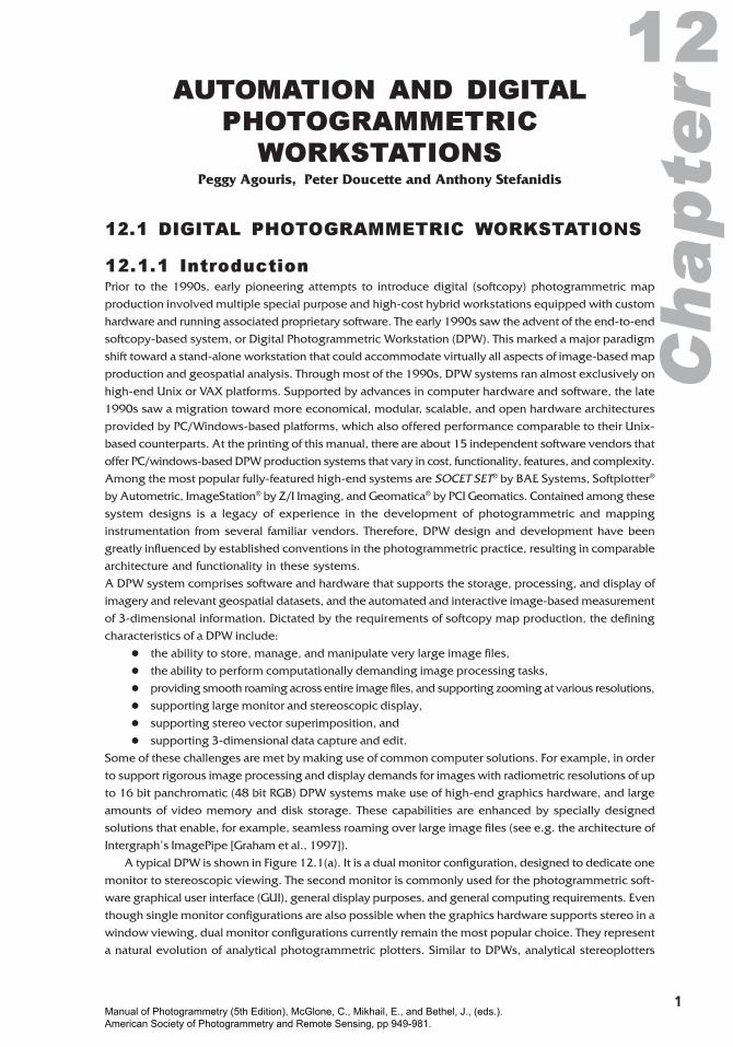
A typical DPW is shown in Figure 12.1(a). It is a dual monitor configuration, designed to dedicate onemonitor to stereoscopic viewing. The second monitor is commonly used for the photogrammetric soft-ware graphical user interface (GUI), general display purposes, and general computing requirements. Eventhough single monitor configurations are also possible when the graphics hardware supports stereo in awindow viewing, dual monitor configurations currently remain the most popular choice. They representa natural evolution of analytical photogrammetric plotters. Similar to DPWs, analytical stereoplotters
Manual of Photogrammetry (5th Edition), McGlone, C., Mikhail, E., and Bethel, J., (eds.). American Society of Photogrammetry and Remote Sensing, pp 949-981.
2 Chapter 12
made use of a monitor dedicated to GUI andsoftware control. The stereo displaying moni-tor of a DPW (and corresponding eyewear)can be considered the counterpart of thecomplex electro-optical viewing system ofan analytical stereoplotter with its ocularsand corresponding prisms. It allows the op-erator to view stereoscopically a window inthe overlapping area of a stereopair. As theimages are available in a DPW in softcopyformat (as computer files) instead of actualfilm, the complex electromechanical mecha-nism used to control movement in an ana-lytical stereoplotter is obsolete for a DPW,replaced by computer operations that generate pixel addresses within a file and accessing the corre-sponding information. The 3-dimensional measuring device (a.k.a. turtle) of an analytical stereoplotter isreplaced by specialized 3-dimensional mouse designs that are available to facilitate the extraction of x,y, z coordinates. These 3-dimensional mouse designs may range from simple mouse-and-trackball con-figurations to more complex specially designed devices such as Leica Geosystems’ TopoMouse shown inFigure 12.1(b). The TopoMouse has several programmable buttons, and a large thumbwheel to adjust thez-coordinate, and complements standard PC input devices to control roaming and measuring in bothsingle image and stereo mode.
Beyond the above-mentioned effects that the availability of softcopy imagery has had on the designof DPW configurations, the most dramatic effect of this transition has been the increased degree ofautomation of photogrammetric operations. Whereas automation in analytical stereoplotters was limitedto driving the stereoplotter stage to specific locations, in DPWs automation has affected practically allparts of the photogrammetric process, from orientation to orthophoto generation. This automation isaddressed in Sections 12.2 - 12.4 of this manual.
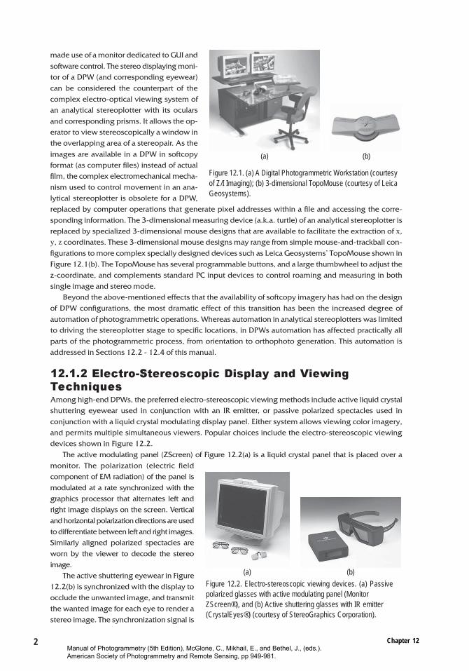
12.1.2 Electro-Stereoscopic Display and ViewingTechniquesAmong high-end DPWs, the preferred electro-stereoscopic viewing methods include active liquid crystalshuttering eyewear used in conjunction with an IR emitter, or passive polarized spectacles used inconjunction with a liquid crystal modulating display panel. Either system allows viewing color imagery,and permits multiple simultaneous viewers. Popular choices include the electro-stereoscopic viewingdevices shown in Figure 12.2.
The active modulating panel (ZScreen) of Figure 12.2(a) is a liquid crystal panel that is placed over amonitor. The polarization (electric fieldcomponent of EM radiation) of the panel ismodulated at a rate synchronized with thegraphics processor that alternates left andright image displays on the screen. Verticaland horizontal polarization directions are usedto differentiate between left and right images.Similarly aligned polarized spectacles areworn by the viewer to decode the stereoimage.
The active shuttering eyewear in Figure12.2(b) is synchronized with the display toocclude the unwanted image, and transmitthe wanted image for each eye to render astereo image. The synchronization signal is
Figure 12.1. (a) A Digital Photogrammetric Workstation (courtesyof Z/I Imaging); (b) 3-dimensional TopoMouse (courtesy of LeicaGeosystems).
(a) (b)
Figure 12.2. Electro-stereoscopic viewing devices. (a) Passivepolarized glasses with active modulating panel (MonitorZScreen®), and (b) Active shuttering glasses with IR emitter(CrystalEyes®) (courtesy of StereoGraphics Corporation).
(a) (b)
Manual of Photogrammetry (5th Edition), McGlone, C., Mikhail, E., and Bethel, J., (eds.). American Society of Photogrammetry and Remote Sensing, pp 949-981.
Automation and Digital Photogrammetric Workstations 3
transmitted to the eyewear via an IR signal that originates from an emitter that interfaces with thegraphics hardware.
In either case, the stereoscopic display technique used is referred to as time-multiplexing or field-sequential. A field represents image information allocated in video memory to be drawn to the displaymonitor during a single refresh cycle. In such an approach, parallax information is provided to the eye byrapidly alternating between the left and right images on the monitor. The images must be refreshed at asufficient rate (typically 120 fields per second, to achieve 60 fields per second per eye), in order to generatea flicker-free stereoscopic image. Today, stereo-ready high-end graphics cards and monitors that use atleast a double-buffering technique to provide refresh rates up to 120 fields per second are readily availablefor most computing platforms. Such graphics cards are equipped with a connector that provides an outputsynchronization signal for electronic shuttering devices such as an IR emitter or monitor panel.
Stereoscopic viewing solutions also exist for graphics hardware that is not stereo-ready. Known asthe above-and-below format, the method uses two vertically arranged subfields that are above andbelow each other, and squeezed top to bottom by a factor of two in a single field. A sync-doubling emitteradds the missing synchronization pulses for a graphics hardware running at a nominal rate of 60 fields persecond, thus doubling the rate for the desired flicker-free stereo image. As a result of altering the syncrate of the monitor, above-and-below stereoscopic applications must run at full-screen. The stereographics hardware automatically unsqueezes the image in the vertical so the stereo image has theexpected aspect ratio. A trade-off with this approach is that the vertical resolution of the stereo imageis effectively reduced by a factor of 2, since the pixels are stretched in the vertical directional. Nonetheless,the above-and-below format provides a workable solution for non-stereo-ready graphics hardware.
When video memory is limited, a relatively low-cost technique for generating a stereo image is tointerlace left and right images on odd and even field lines (e.g., left image drawn on lines 1, 3, 5…etc.,and right image on lines 2, 4, 6…etc.). Shuttering eyewear is synchronized with the refresh rate of theodd and even field lines in order to decode a stereo image for the viewer. The drawbacks of interlacedstereo include a degradation of vertical resolution by a factor of 2, more noticeable flicker, and applicationsthat are limited to full screen stereo mode.
For state-of-the-art stereo viewing capabilities, high-end 3-dimensional graphics hardware designsoffer what is known as quad buffered stereo (QBS). Once available only on Unix workstations, QBS hasnow become common place on PCs. QBS can be understood as a simple extension of double-bufferedanimation, i.e., during the display of one video image, the image to follow is concurrently drawn to amemory buffer. The result is a faster, and thus smoother transition between image sequences. Double-buffering is exploited in stereoscopic display techniques to speed up the transitions between left andright images. QBS extends this concept even further by dividing the graphics memory into four buffers,such that one pair of buffers is the display pair, while the other is the rendering pair. The result is vastlyimproved stereo viewing quality in terms of smoothness during image roaming, as well as renderingreal-time superimposed vectors that are always current. A significant advantage of QBS is that it allowsfor multiple stereo-in-a-window (SIAW) renderings. That is, a user has access to other application windowswhile rendering stereo displays in one or more windows on a single monitor.
In an ideal stereoscopic system, each eye sees only the image intended for it. Electro-stereoscopicviewing techniques are susceptible to a certain amount of crosstalk, i.e., when either eye is allowed tosee the image for the other eye, to some extent. The principal source of crosstalk in electro-stereoscopicdisplay is CRT phosphor afterglow, or ghosting. Following the display of the right image, its afterglowwill persist to some extent during the display of the left image, and vice-versa. Ghosting is kept at atolerable level by using sufficiently low parallax angles. As a general rule of thumb, parallax angles arekept under 1.5° for comfortable stereo viewing with a typical workstation configuration (StereoGraphics,1997). The parallax angle θ is defined as
(12.1)
where P is the distance between right and left-eye projections of a given image point, and d is the
Manual of Photogrammetry (5th Edition), McGlone, C., Mikhail, E., and Bethel, J., (eds.). American Society of Photogrammetry and Remote Sensing, pp 949-981.
4 Chapter 12
distance between the viewer’s eye plane and the display screen. Latest advances in stereoscopicviewing devices include autostereoscopic solutions that require no specialized eyewear, rendering theirdisplay on a liquid crystal flat-screen monitor.
12.2 AUTOMATED ORIENTATIONS IN A DPW
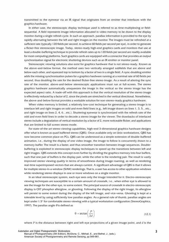
12.2.1 Photogrammetric Mapping WorkflowThe structure of the typical photogrammetric mapping workflow remains largely unchanged, as imagesare oriented and subsequently analyzed to produce geospatial information. Figure 12.3 is a schematicdescription of this workflow, identifying two groups of operations that make use of digital imagery. Themiddle column group comprises operations that relate images to other images and to a referencecoordinate system, namely orientations and triangulation. The right-hand column comprises operationsthat generate geospatial information: producing digital elevation models (DEMs) and orthophotos, andproceeding with GIS generation or updates through feature extraction.
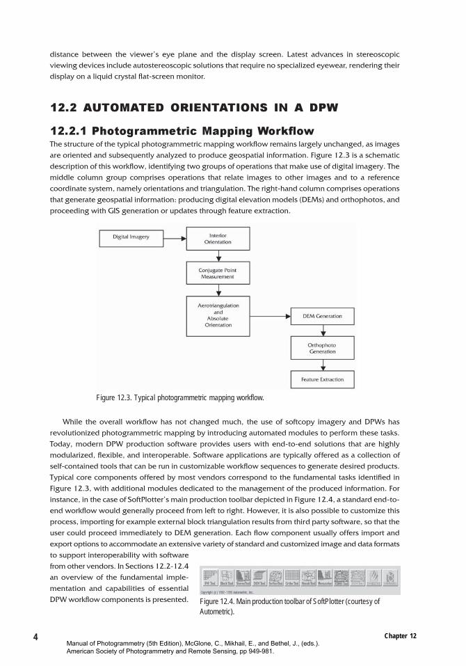
While the overall workflow has not changed much, the use of softcopy imagery and DPWs hasrevolutionized photogrammetric mapping by introducing automated modules to perform these tasks.Today, modern DPW production software provides users with end-to-end solutions that are highlymodularized, flexible, and interoperable. Software applications are typically offered as a collection ofself-contained tools that can be run in customizable workflow sequences to generate desired products.Typical core components offered by most vendors correspond to the fundamental tasks identified inFigure 12.3, with additional modules dedicated to the management of the produced information. Forinstance, in the case of SoftPlotter’s main production toolbar depicted in Figure 12.4, a standard end-to-end workflow would generally proceed from left to right. However, it is also possible to customize thisprocess, importing for example external block triangulation results from third party software, so that theuser could proceed immediately to DEM generation. Each flow component usually offers import andexport options to accommodate an extensive variety of standard and customized image and data formatsto support interoperability with softwarefrom other vendors. In Sections 12.2-12.4an overview of the fundamental imple-mentation and capabilities of essentialDPW workflow components is presented.
Figure 12.3. Typical photogrammetric mapping workflow.
Figure 12.4. Main production toolbar of SoftPlotter (courtesy ofAutometric).
Manual of Photogrammetry (5th Edition), McGlone, C., Mikhail, E., and Bethel, J., (eds.). American Society of Photogrammetry and Remote Sensing, pp 949-981.
Automation and Digital Photogrammetric Workstations 5
12.2.2 Interior Orientation in a DPWWhile digital cameras are becoming the standard in close-range applications, aerial mapping missionscommonly make use of analog cameras. The use of advanced high resolution digital sensors inphotogrammetric applications is still at an experimental stage [Fraser et al., 2002]. Aerial photographscaptured in analog format (using film cameras) are subsequently scanned to produce softcopy counterpartsof the original diapositives. These digitized diapositives are the common input to a DPW workflow. In thisset-up, interior orientation comprises two transformations:
� a transformation from the digital image pixel coordinate system (rows and columns) to the photocoordinate system of the analog image, as it is defined by the fiducial marks, and
� the definition of the camera model by selecting the corresponding camera calibration parameters,to support the eventual transformation from photo coordinates to the object space.
The second task is addressed during projectpreparation by selecting the appropriate cameracalibration file, similar to the way this information isselected in an analytical stereoplotter. This file includesthe geometric parameters that define the specificimage formation process, e.g. camera constant, fiducialmark coordinates, distortion parameters. Thisinformation is used later during aerotriangulation toreconstruct the image formation geometry using thecollinearity equations (Chapters 3 and 11).
The novelty introduced by the use of DPWs inrecovering interior orientation is related to the firsttransformation, namely from pixel (r,c) to the photo(xp,yp) coordinate system, which requires theidentification and precise measurement of fiducial marksin the digital image. Since fiducial marks are well-definedtargets, this process is highly suitable for full automation.
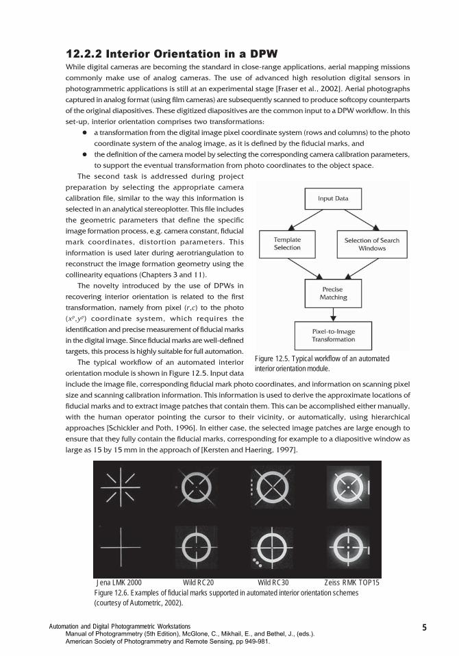
The typical workflow of an automated interiororientation module is shown in Figure 12.5. Input datainclude the image file, corresponding fiducial mark photo coordinates, and information on scanning pixelsize and scanning calibration information. This information is used to derive the approximate locations offiducial marks and to extract image patches that contain them. This can be accomplished either manually,with the human operator pointing the cursor to their vicinity, or automatically, using hierarchicalapproaches [Schickler and Poth, 1996]. In either case, the selected image patches are large enough toensure that they fully contain the fiducial marks, corresponding for example to a diapositive window aslarge as 15 by 15 mm in the approach of [Kersten and Haering, 1997].
Figure 12.5. Typical workflow of an automatedinterior orientation module.
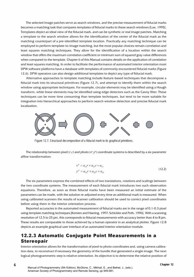
Jena LMK 2000 Wild RC20 Wild RC30 Zeiss RMK TOP15Figure 12.6. Examples of fiducial marks supported in automated interior orientation schemes(courtesy of Autometric, 2002).
Manual of Photogrammetry (5th Edition), McGlone, C., Mikhail, E., and Bethel, J., (eds.). American Society of Photogrammetry and Remote Sensing, pp 949-981.
6 Chapter 12
The selected image patches serve as search windows, and the precise measurement of fiducial marksbecomes a matching task that compares templates of fiducial marks to these search windows [Lue, 1995].Templates depict an ideal view of the fiducial mark, and can be synthetic or real image patches. Matchinga template to the search window allows for the identification of the center of the fiducial mark as thematching counterpart of a pre-identified template location. Practically any matching technique can beemployed to perform template-to-image matching, but the most popular choices remain correlation andleast squares matching techniques. They allow for the identification of a location within the searchwindow that offers the maximum correlation coefficient or minimum sum of squared gray value differenceswhen compared to the template. Chapter 6 of this Manual contains details on the application of correlationand least squares matching. In order to facilitate the performance of automated interior orientation mostDPW software platforms have a database with templates of commonly encountered fiducial marks (Figure12.6). DPW operators can also design additional templates to depict any type of fiducial mark.
Alternative approaches to template matching include feature-based techniques that decompose afiducial mark into its structural primitives (Figure 12.7), and attempt to identify them within the searchwindow using appropriate techniques. For example, circular elements may be identified using a Houghtransform, while linear elements may be identified using edge detectors such as the Canny filter. Thesetechniques can be more time consuming than template techniques, but tend to be more suitable forintegration into hierarchical approaches to perform search window detection and precise fiducial marklocalization.
The relationship between pixel (r,c) and photo (xp,yp) coordinate systems is described by a six parameteraffine transformation:
(12.2)
The six parameters express the combined effects of two translations, rotations and scalings betweenthe two coordinate systems. The measurement of each fiducial mark introduces two such observationequations. Therefore, as soon as three fiducial marks have been measured an initial estimate of theparameters can be made, with the solution re-adjusted every time an additional mark is measured. Whenusing calibrated scanners the results of scanner calibration should be used to correct pixel coordinatesbefore using them in the interior orientation process.
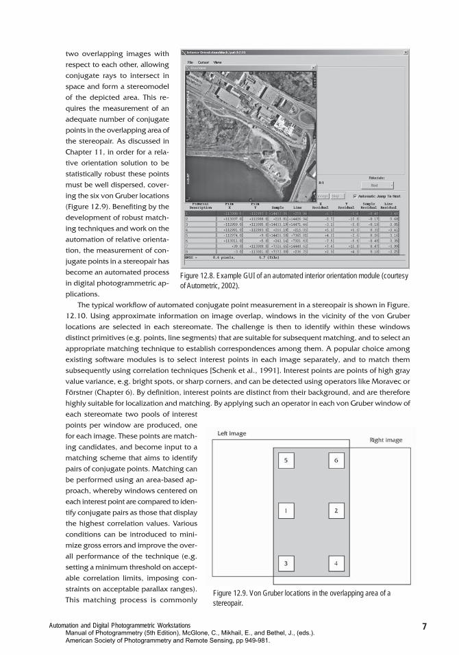
Reported accuracies in the automated measurement of fiducial marks are in the range of 0.1-0.3 pixelusing template matching techniques [Kersten and Haering, 1997; Schickler and Poth, 1996]. With a scanningresolution of 12.5 to 25 µm, this corresponds to fiducial measurements with accuracy better than 4 to 8 µm.These results are comparable to those achieved by a human operator in an analytical plotter. Figure 12.8depicts an example graphical user interface of an automated interior orientation module.
12.2.3 Automatic Conjugate Point Measurements in a
StereopairInterior orientation allows for the transformation of pixel to photo coordinates and, using camera calibra-tion data, to reconstruct if necessary the geometry of the bundle that generated a single image. The nextlogical photogrammetric step is relative orientation. Its objective is to determine the relative position of
Figure 12.7. Structural decomposition of a fiducial mark to its graphical primitives.
Manual of Photogrammetry (5th Edition), McGlone, C., Mikhail, E., and Bethel, J., (eds.). American Society of Photogrammetry and Remote Sensing, pp 949-981.
Automation and Digital Photogrammetric Workstations 7
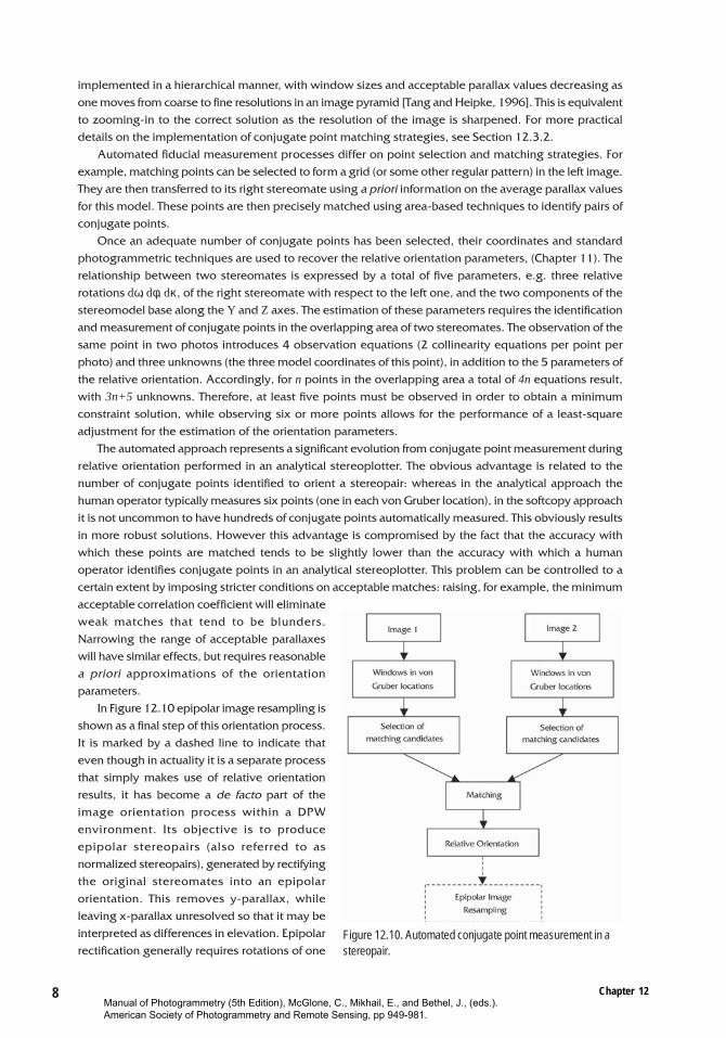
two overlapping images withrespect to each other, allowingconjugate rays to intersect inspace and form a stereomodelof the depicted area. This re-quires the measurement of anadequate number of conjugatepoints in the overlapping area ofthe stereopair. As discussed inChapter 11, in order for a rela-tive orientation solution to bestatistically robust these pointsmust be well dispersed, cover-ing the six von Gruber locations(Figure 12.9). Benefiting by thedevelopment of robust match-ing techniques and work on theautomation of relative orienta-tion, the measurement of con-jugate points in a stereopair hasbecome an automated processin digital photogrammetric ap-plications.
The typical workflow of automated conjugate point measurement in a stereopair is shown in Figure.12.10. Using approximate information on image overlap, windows in the vicinity of the von Gruberlocations are selected in each stereomate. The challenge is then to identify within these windowsdistinct primitives (e.g. points, line segments) that are suitable for subsequent matching, and to select anappropriate matching technique to establish correspondences among them. A popular choice amongexisting software modules is to select interest points in each image separately, and to match themsubsequently using correlation techniques [Schenk et al., 1991]. Interest points are points of high grayvalue variance, e.g. bright spots, or sharp corners, and can be detected using operators like Moravec orFörstner (Chapter 6). By definition, interest points are distinct from their background, and are thereforehighly suitable for localization and matching. By applying such an operator in each von Gruber window ofeach stereomate two pools of interestpoints per window are produced, onefor each image. These points are match-ing candidates, and become input to amatching scheme that aims to identifypairs of conjugate points. Matching canbe performed using an area-based ap-proach, whereby windows centered oneach interest point are compared to iden-tify conjugate pairs as those that displaythe highest correlation values. Variousconditions can be introduced to mini-mize gross errors and improve the over-all performance of the technique (e.g.setting a minimum threshold on accept-able correlation limits, imposing con-straints on acceptable parallax ranges).This matching process is commonly
Figure 12.8. Example GUI of an automated interior orientation module (courtesyof Autometric, 2002).
Figure 12.9. Von Gruber locations in the overlapping area of astereopair.
Manual of Photogrammetry (5th Edition), McGlone, C., Mikhail, E., and Bethel, J., (eds.). American Society of Photogrammetry and Remote Sensing, pp 949-981.
8 Chapter 12
implemented in a hierarchical manner, with window sizes and acceptable parallax values decreasing asone moves from coarse to fine resolutions in an image pyramid [Tang and Heipke, 1996]. This is equivalentto zooming-in to the correct solution as the resolution of the image is sharpened. For more practicaldetails on the implementation of conjugate point matching strategies, see Section 12.3.2.
Automated fiducial measurement processes differ on point selection and matching strategies. Forexample, matching points can be selected to form a grid (or some other regular pattern) in the left image.They are then transferred to its right stereomate using a priori information on the average parallax valuesfor this model. These points are then precisely matched using area-based techniques to identify pairs ofconjugate points.
Once an adequate number of conjugate points has been selected, their coordinates and standardphotogrammetric techniques are used to recover the relative orientation parameters, (Chapter 11). Therelationship between two stereomates is expressed by a total of five parameters, e.g. three relativerotations dω, dφ, dκ, of the right stereomate with respect to the left one, and the two components of thestereomodel base along the Y and Z axes. The estimation of these parameters requires the identificationand measurement of conjugate points in the overlapping area of two stereomates. The observation of thesame point in two photos introduces 4 observation equations (2 collinearity equations per point perphoto) and three unknowns (the three model coordinates of this point), in addition to the 5 parameters ofthe relative orientation. Accordingly, for n points in the overlapping area a total of 4n equations result,with 3n+5 unknowns. Therefore, at least five points must be observed in order to obtain a minimumconstraint solution, while observing six or more points allows for the performance of a least-squareadjustment for the estimation of the orientation parameters.
The automated approach represents a significant evolution from conjugate point measurement duringrelative orientation performed in an analytical stereoplotter. The obvious advantage is related to thenumber of conjugate points identified to orient a stereopair: whereas in the analytical approach thehuman operator typically measures six points (one in each von Gruber location), in the softcopy approachit is not uncommon to have hundreds of conjugate points automatically measured. This obviously resultsin more robust solutions. However this advantage is compromised by the fact that the accuracy withwhich these points are matched tends to be slightly lower than the accuracy with which a humanoperator identifies conjugate points in an analytical stereoplotter. This problem can be controlled to acertain extent by imposing stricter conditions on acceptable matches: raising, for example, the minimumacceptable correlation coefficient will eliminateweak matches that tend to be blunders.Narrowing the range of acceptable parallaxeswill have similar effects, but requires reasonablea priori approximations of the orientationparameters.
In Figure 12.10 epipolar image resampling isshown as a final step of this orientation process.It is marked by a dashed line to indicate thateven though in actuality it is a separate processthat simply makes use of relative orientationresults, it has become a de facto part of theimage orientation process within a DPWenvironment. Its objective is to produceepipolar stereopairs (also referred to asnormalized stereopairs), generated by rectifyingthe original stereomates into an epipolarorientation. This removes y-parallax, whileleaving x-parallax unresolved so that it may beinterpreted as differences in elevation. Epipolarrectification generally requires rotations of one
Figure 12.10. Automated conjugate point measurement in astereopair.
Manual of Photogrammetry (5th Edition), McGlone, C., Mikhail, E., and Bethel, J., (eds.). American Society of Photogrammetry and Remote Sensing, pp 949-981.
Automation and Digital Photogrammetric Workstations 9
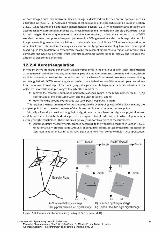
or both images such that horizontal lines of imagery displayed on the screen are epipolar lines asillustrated in Figure 12.11. A detailed mathematical derivation of the procedure can be found in Section3.2.2.7, while resampling is addressed in more detail in Section 12.3.3. With digital images, rotations areaccomplished via a resampling process that must guarantee the same ground sample distance per pixelfor both images. This technique, referred to as epipolar resampling, has become an essential part of DPWworkflow because it supports subsequent processes like DEM generation and orthophoto production. Asimage resampling involves interpolation to derive each new pixel, it is a CPU intensive operation. Inorder to alleviate this problem, techniques such as on-the-fly epipolar resampling have been developed(used e.g. in ImageStation) to dynamically localize the resampling process to regions of interest. Thiseliminates the need to generate entire epipolar resampled images prior to display and reduces theamount of disk storage overhead.
12.2.4 AerotriangulationIn modern DPWs the relative orientation workflow presented in the previous section is not implementedas a separate stand-alone module, but rather as part of a broader point measurement and triangulationmodule. However, it provides the theoretical and practical basis of automated point measurement duringaerotriangulation in DPWs. Aerotriangulation is often characterized as one of the more complex proceduresin terms of user knowledge of the underlying principles of a photogrammetric block adjustment. Itsobjective is to relate multiple images to each other in order to:
� recover the complete orientation parameters of each image in the block, namely the (X0,Y
0,Z
0)
coordinates of the exposure station and the ω,φ,κ rotations, and to� determine the ground coordinates (X,Y,Z) of points observed in them.
This requires the measurement of conjugate points in the overlapping areas of the block imagery (tieand pass points), and the measurement of the photo coordinates of depicted control points.
Virtually all vendors provide triangulation algorithms that are based on rigorous physical sensormodels and the well-established principles of least squares bundle adjustment in which all parametersare fully weight-constrained. These modules typically support two types of measurements:
� Automatic Point Measurements: proceed according to the workflow described in Section 12.2.3to automatically produce large amounts of conjugate points. To accommodate the needs ofaerotriangulation, matching tools have been extended from stereo to multi-stage application.
Figure 12.11. Pairwise epipolar rectification (courtesy of BAE Systems, 2001).
Manual of Photogrammetry (5th Edition), McGlone, C., Mikhail, E., and Bethel, J., (eds.). American Society of Photogrammetry and Remote Sensing, pp 949-981.
10 Chapter 12
The proposed techniques include the extension of least squares matching to multi-imageapplication and their integration with block adjustment [Agouris, 1993; Agouris and Schenk,1996], and the introduction of graph-based techniques to combine sequences of stereo matchingresults in a block adjustment [Tsingas, 1994].
� Interactive Point Measurements: supports user-controlled measurements for the identificationand measurement in a semi-automatic mode for specific points, especially ground control points.
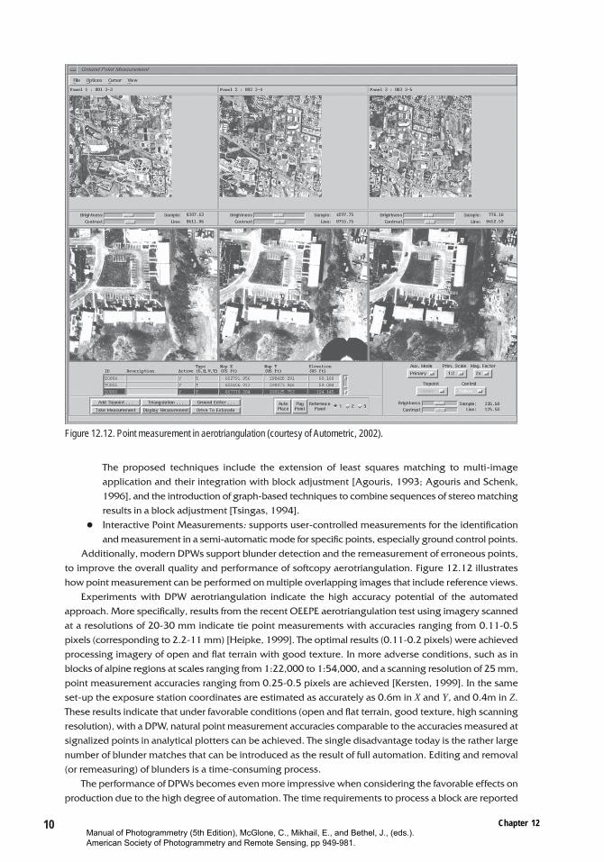
Additionally, modern DPWs support blunder detection and the remeasurement of erroneous points,to improve the overall quality and performance of softcopy aerotriangulation. Figure 12.12 illustrateshow point measurement can be performed on multiple overlapping images that include reference views.
Experiments with DPW aerotriangulation indicate the high accuracy potential of the automatedapproach. More specifically, results from the recent OEEPE aerotriangulation test using imagery scannedat a resolutions of 20-30 mm indicate tie point measurements with accuracies ranging from 0.11-0.5pixels (corresponding to 2.2-11 mm) [Heipke, 1999]. The optimal results (0.11-0.2 pixels) were achievedprocessing imagery of open and flat terrain with good texture. In more adverse conditions, such as inblocks of alpine regions at scales ranging from 1:22,000 to 1:54,000, and a scanning resolution of 25 mm,point measurement accuracies ranging from 0.25-0.5 pixels are achieved [Kersten, 1999]. In the sameset-up the exposure station coordinates are estimated as accurately as 0.6m in X and Y, and 0.4m in Z.These results indicate that under favorable conditions (open and flat terrain, good texture, high scanningresolution), with a DPW, natural point measurement accuracies comparable to the accuracies measured atsignalized points in analytical plotters can be achieved. The single disadvantage today is the rather largenumber of blunder matches that can be introduced as the result of full automation. Editing and removal(or remeasuring) of blunders is a time-consuming process.
The performance of DPWs becomes even more impressive when considering the favorable effects onproduction due to the high degree of automation. The time requirements to process a block are reported
Figure 12.12. Point measurement in aerotriangulation (courtesy of Autometric, 2002).
Manual of Photogrammetry (5th Edition), McGlone, C., Mikhail, E., and Bethel, J., (eds.). American Society of Photogrammetry and Remote Sensing, pp 949-981.
Automation and Digital Photogrammetric Workstations 11
to range from 10-20 minutes per image considering only operator-assisted processes and excludingbatch processes, scanning, and control preparation [Kersten, 1999]. This represents a significantimprovement compared to analytical processes.
12.2.5. Generalized Sensor ModelsThe sensor model establishes the functional relationship between image and object space. A physical orrigorous sensor model is used to represent the physical imaging process, making use of information on thesensor’s position and orientation. Classical sensors employed in photogrammetric missions are commonlymodeled through the collinearity condition. By contrast, a generalized or replacement sensor model doesnot include sensor position and orientation information. Rather, a general polynomial function is used torepresent the transformation between image and object space. While a general polynomial function is lessaccurate than a physical model, it offers significantly faster computational processing. It is also completelyindependent of the sensor platform, and thus particularly suitable for today’s ever increasing variety ofimage sources. A common practice used in DPW software implementations is to use a physical sensormodel (when available) during aerotriangulation only. Then, a set of rational functions that approximate theprojective geometry is derived from the physical model solution. These rational functions then serve as areplacement sensor model that can provide for faster or real-time implementations of subsequent workstationoperations (e.g., DEM generation, orthoimage generation, and feature extraction).
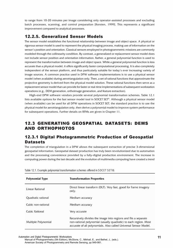
High-end DPW software vendors provide several polynomial transformation schemes. Table 12.1lists available options for the fast sensor model tool in SOCET SET®. Although a physical sensor model(when available) can be used for all DPW operations in SOCET SET, the standard practice is to use thephysical model for aerotriangulation only, then derive a polynomial model to improve system performancefor subsequent operations. Further details on RFMs are given in Chapter 11.
12.3 GENERATING GEOSPATIAL DATASETS: DEMS
AND ORTHOPHOTOS
12.3.1 Digital Photogrammetric Production of GeospatialDatasetsThe completion of triangulation in a DPW allows the subsequent extraction of precise 3-dimensionalgeospatial information. Geospatial dataset production has truly been revolutionized due to automationand the processing convenience provided by a fully-digital production environment. The increase incomputing power during the last decade and the evolution of multimedia computing have created a trend
Table 12.1. Example polynomial transformation schemes offered in SOCET SET®.
Manual of Photogrammetry (5th Edition), McGlone, C., Mikhail, E., and Bethel, J., (eds.). American Society of Photogrammetry and Remote Sensing, pp 949-981.
12 Chapter 12
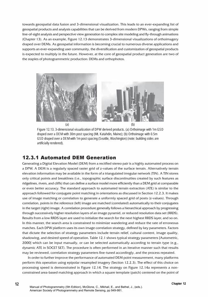
towards geospatial data fusion and 3-dimensional visualization. This leads to an ever-expanding list ofgeospatial products and analysis capabilities that can be derived from modern DPWs, ranging from simpleline-of-sight analysis and perspective view generation to complex site modeling and fly-through animations(Chapter 13). As an example, Figure 12.13 demonstrates 3-dimensional visualizations of orthoimagerydraped over DEMs. As geospatial information is becoming crucial to numerous diverse applications andsupports an ever-expanding user community, the diversification and customization of geospatial productsis expected to multiply in the future. However, at the core of geospatial product generation are two ofthe staples of photogrammetric production: DEMs and orthophotos.
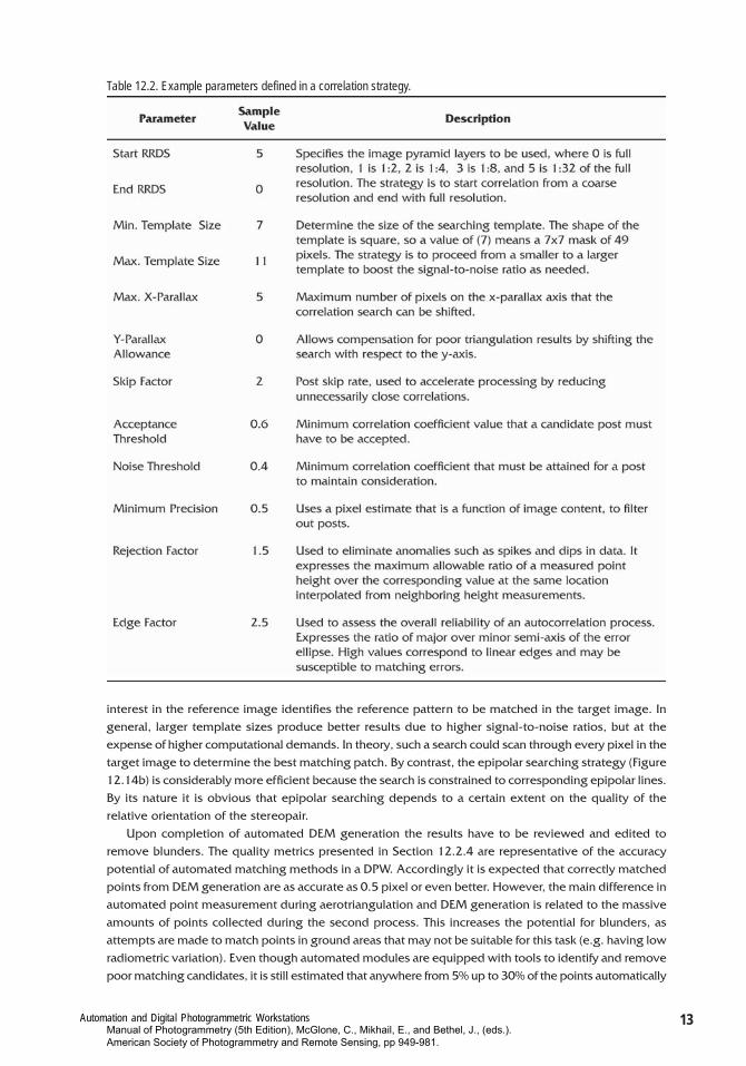
12.3.1 Automated DEM GenerationGenerating a Digital Elevation Model (DEM) from a rectified stereo pair is a highly automated process ona DPW. A DEM is a regularly spaced raster grid of z-values of the surface terrain. Alternatively terrainelevation information may be available in the form of a triangulated irregular network (TIN). A TIN storesonly critical points and breaklines (i.e., topographic surface discontinuities created by such features asridgelines, rivers, and cliffs) that can define a surface model more efficiently than a DEM grid at comparableor even better accuracy. The standard approach to automated terrain extraction (ATE) is similar to theapproach followed for conjugate point matching in orientations as discussed in Section 12.2.3. It makesuse of image matching or correlation to generate a uniformly spaced grid of posts (z-values). Throughcorrelation, points in the reference (left) image are matched (correlated) automatically to their conjugatesin the target (right) image. A correlation procedure generally follows a hierarchical approach by progressingthrough successively higher resolution layers of an image pyramid, or reduced resolution data set (RRDS).Results from a low RRDS layer are used to initialize the search for the next highest RRDS layer, and so on.In this manner, the search area is constrained to minimize wandering and reduce the rate of erroneousmatches. Each DPW platform uses its own image correlation strategy, defined by key parameters. Factorsthat dictate the selection of strategy parameters include terrain relief, cultural content, image quality,shadowing, and desired speed of operation. Table 12.1 shows typical strategy parameters [Autometric,2000] which can be input manually, or can be selected automatically according to terrain type (e.g.,dynamic ATE in SOCET SET). The procedure is often performed in an iterative manner such that resultsmay be reviewed, correlation strategy parameters fine-tuned accordingly, and the process repeated.
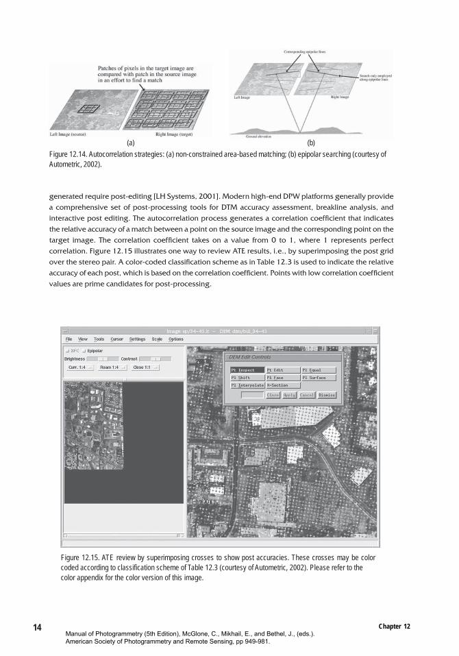
In order to further improve the performance of automated DEM point measurement, many platformsperform this operation using epipolar resampled imagery (Section 12.2.3). The effect of this choice onprocessing speed is demonstrated in Figure 12.14. The strategy on Figure 12.14a represents a non-constrained area-based matching approach in which a square template (patch) centered on the point of
(a) (b)Figure 12.13. 3-dimensional visualization of DPW derived products. (a) Orthoimage with 1m GSDdraped over a DEM with 30m post spacing (Mt. Katahdin, Maine); (b) Orthoimage with 0.5mGSD draped over a DEM with 1m post spacing (Seattle, Washington) (note: building sides areartificially rendered).
Manual of Photogrammetry (5th Edition), McGlone, C., Mikhail, E., and Bethel, J., (eds.). American Society of Photogrammetry and Remote Sensing, pp 949-981.
Automation and Digital Photogrammetric Workstations 13
interest in the reference image identifies the reference pattern to be matched in the target image. Ingeneral, larger template sizes produce better results due to higher signal-to-noise ratios, but at theexpense of higher computational demands. In theory, such a search could scan through every pixel in thetarget image to determine the best matching patch. By contrast, the epipolar searching strategy (Figure12.14b) is considerably more efficient because the search is constrained to corresponding epipolar lines.By its nature it is obvious that epipolar searching depends to a certain extent on the quality of therelative orientation of the stereopair.
Upon completion of automated DEM generation the results have to be reviewed and edited toremove blunders. The quality metrics presented in Section 12.2.4 are representative of the accuracypotential of automated matching methods in a DPW. Accordingly it is expected that correctly matchedpoints from DEM generation are as accurate as 0.5 pixel or even better. However, the main difference inautomated point measurement during aerotriangulation and DEM generation is related to the massiveamounts of points collected during the second process. This increases the potential for blunders, asattempts are made to match points in ground areas that may not be suitable for this task (e.g. having lowradiometric variation). Even though automated modules are equipped with tools to identify and removepoor matching candidates, it is still estimated that anywhere from 5% up to 30% of the points automatically
Table 12.2. Example parameters defined in a correlation strategy.
Manual of Photogrammetry (5th Edition), McGlone, C., Mikhail, E., and Bethel, J., (eds.). American Society of Photogrammetry and Remote Sensing, pp 949-981.
14 Chapter 12
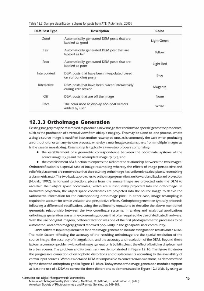
generated require post-editing [LH Systems, 2001]. Modern high-end DPW platforms generally providea comprehensive set of post-processing tools for DTM accuracy assessment, breakline analysis, andinteractive post editing. The autocorrelation process generates a correlation coefficient that indicatesthe relative accuracy of a match between a point on the source image and the corresponding point on thetarget image. The correlation coefficient takes on a value from 0 to 1, where 1 represents perfectcorrelation. Figure 12.15 illustrates one way to review ATE results, i.e., by superimposing the post gridover the stereo pair. A color-coded classification scheme as in Table 12.3 is used to indicate the relativeaccuracy of each post, which is based on the correlation coefficient. Points with low correlation coefficientvalues are prime candidates for post-processing.
(a) (b)
Figure 12.14. Autocorrelation strategies: (a) non-constrained area-based matching; (b) epipolar searching (courtesy ofAutometric, 2002).
Figure 12.15. ATE review by superimposing crosses to show post accuracies. These crosses may be colorcoded according to classification scheme of Table 12.3 (courtesy of Autometric, 2002). Please refer to thecolor appendix for the color version of this image.
Manual of Photogrammetry (5th Edition), McGlone, C., Mikhail, E., and Bethel, J., (eds.). American Society of Photogrammetry and Remote Sensing, pp 949-981.
Automation and Digital Photogrammetric Workstations 15
12.3.3 Orthoimage GenerationExisting imagery may be resampled to produce a new image that conforms to specific geometric properties,such as the production of a vertical view from oblique imagery. This may be a one-to-one process, wherea single source image is modified into another resampled one, as is commonly the case when producingan orthophoto, or a many-to-one process, whereby a new image contains parts from multiple images asis the case in mosaicking. Resampling is typically a two-step process comprising:
� the establishment of a geometric correspondence between the coordinate systems of thesource image s(x,y) and the resampled image r(x’,y’), and
� the establishment of a function to express the radiometric relationship between the two images.Orthorectification is a special case of image resampling whereby the effects of image perspective andrelief displacement are removed so that the resulting orthoimage has uniformly scaled pixels, resemblinga planimetric map. The two basic approaches to orthoimage generation are forward and backward projection[Novak, 1992]. In forward projection, pixels from the source image are projected onto the DEM toascertain their object space coordinates, which are subsequently projected into the orthoimage. Inbackward projection, the object space coordinates are projected into the source image to derive theradiometric information for the corresponding orthoimage pixel. In either case, image resampling isrequired to account for terrain variation and perspective effects. Orthophoto generation typically proceedsfollowing a differential rectification, using the collinearity equations to describe the above mentionedgeometric relationship between the two coordinate systems. In analog and analytical applicationsorthoimage generation was a time-consuming process that often required the use of dedicated hardware.With the use of digital imagery, orthorectification was one of the first photogrammetric processes to beautomated, and orthoimagery gained renewed popularity in the geospatial user community.
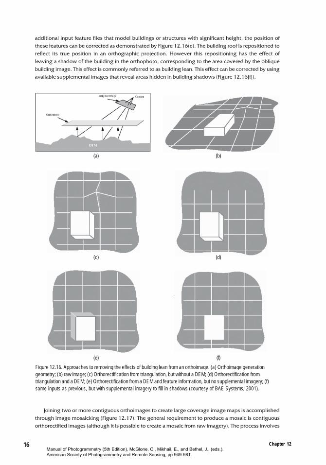
DPW software input requirements for orthoimage generation include triangulation results and a DEM.The main factors affecting the accuracy of the resulting orthoimage are the spatial resolution of thesource image, the accuracy of triangulation, and the accuracy and resolution of the DEM. Beyond thesefactors, a common problem with orthoimage generation is building lean, the effect of building displacementin urban scenes. The problem and its treatment are demonstrated in Figure 12.16. The figure illustratesthe progressive correction of orthophoto distortions and displacements according to the availability ofcertain input sources. Without a detailed DEM it is impossible to correct terrain variations, as demonstratedby the distorted orthophoto grid in Figure 12.16(c). Today most orthoimage generation modules supportat least the use of a DEM to correct for these distortions as demonstrated in Figure 12.16(d). By using as
Table 12.3. Sample classification scheme for posts from ATE [Autometric, 2000].
Manual of Photogrammetry (5th Edition), McGlone, C., Mikhail, E., and Bethel, J., (eds.). American Society of Photogrammetry and Remote Sensing, pp 949-981.
16 Chapter 12
additional input feature files that model buildings or structures with significant height, the position ofthese features can be corrected as demonstrated by Figure 12.16(e). The building roof is repositioned toreflect its true position in an orthographic projection. However this repositioning has the effect ofleaving a shadow of the building in the orthophoto, corresponding to the area covered by the obliquebuilding image. This effect is commonly referred to as building lean. This effect can be corrected by usingavailable supplemental images that reveal areas hidden in building shadows (Figure 12.16[f]).
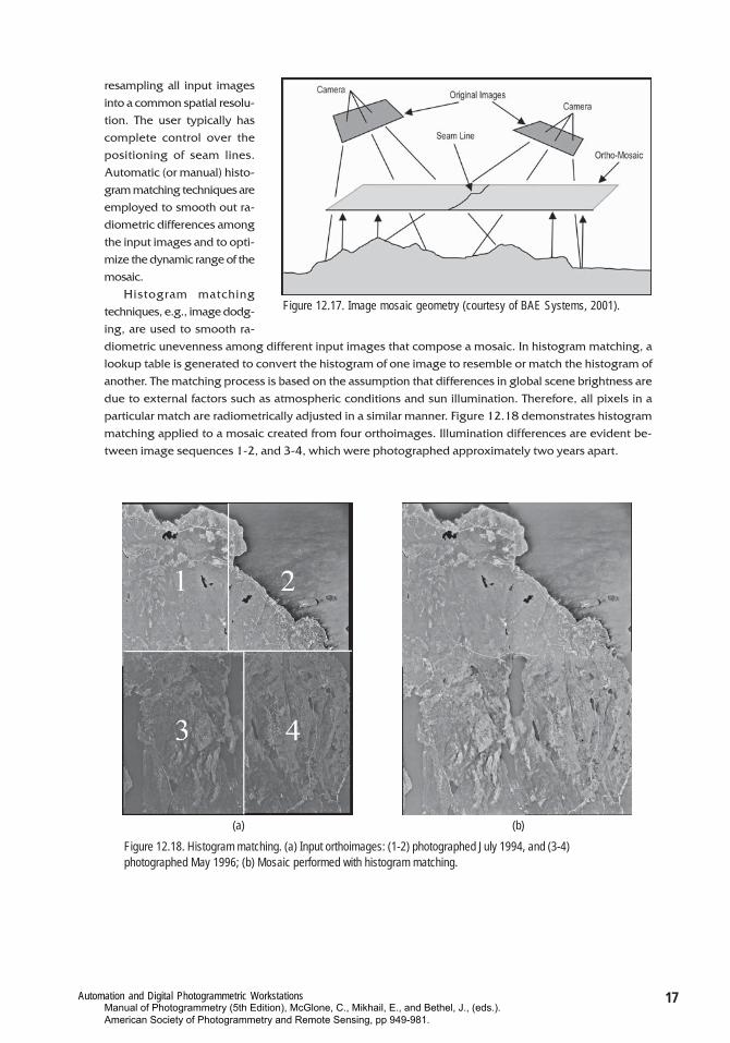
Joining two or more contiguous orthoimages to create large coverage image maps is accomplishedthrough image mosaicking (Figure 12.17). The general requirement to produce a mosaic is contiguousorthorectified images (although it is possible to create a mosaic from raw imagery). The process involves
Figure 12.16. Approaches to removing the effects of building lean from an orthoimage. (a) Orthoimage generationgeometry; (b) raw image; (c) Orthorectification from triangulation, but without a DEM; (d) Orthorectification fromtriangulation and a DEM; (e) Orthorectification from a DEM and feature information, but no supplemental imagery; (f)same inputs as previous, but with supplemental imagery to fill in shadows (courtesy of BAE Systems, 2001).
(a) (b)
(c) (d)
(e) (f)
Manual of Photogrammetry (5th Edition), McGlone, C., Mikhail, E., and Bethel, J., (eds.). American Society of Photogrammetry and Remote Sensing, pp 949-981.
Automation and Digital Photogrammetric Workstations 17
resampling all input imagesinto a common spatial resolu-tion. The user typically hascomplete control over thepositioning of seam lines.Automatic (or manual) histo-gram matching techniques areemployed to smooth out ra-diometric differences amongthe input images and to opti-mize the dynamic range of themosaic.
Histogram matchingtechniques, e.g., image dodg-ing, are used to smooth ra-diometric unevenness among different input images that compose a mosaic. In histogram matching, alookup table is generated to convert the histogram of one image to resemble or match the histogram ofanother. The matching process is based on the assumption that differences in global scene brightness aredue to external factors such as atmospheric conditions and sun illumination. Therefore, all pixels in aparticular match are radiometrically adjusted in a similar manner. Figure 12.18 demonstrates histogrammatching applied to a mosaic created from four orthoimages. Illumination differences are evident be-tween image sequences 1-2, and 3-4, which were photographed approximately two years apart.
Figure 12.17. Image mosaic geometry (courtesy of BAE Systems, 2001).
(a) (b)
Figure 12.18. Histogram matching. (a) Input orthoimages: (1-2) photographed July 1994, and (3-4)photographed May 1996; (b) Mosaic performed with histogram matching.
Manual of Photogrammetry (5th Edition), McGlone, C., Mikhail, E., and Bethel, J., (eds.). American Society of Photogrammetry and Remote Sensing, pp 949-981.
18 Chapter 12
12.4 AUTOMATED FEATURE MEASUREMENTS FOR
GEOSPATIAL APPLICATIONS
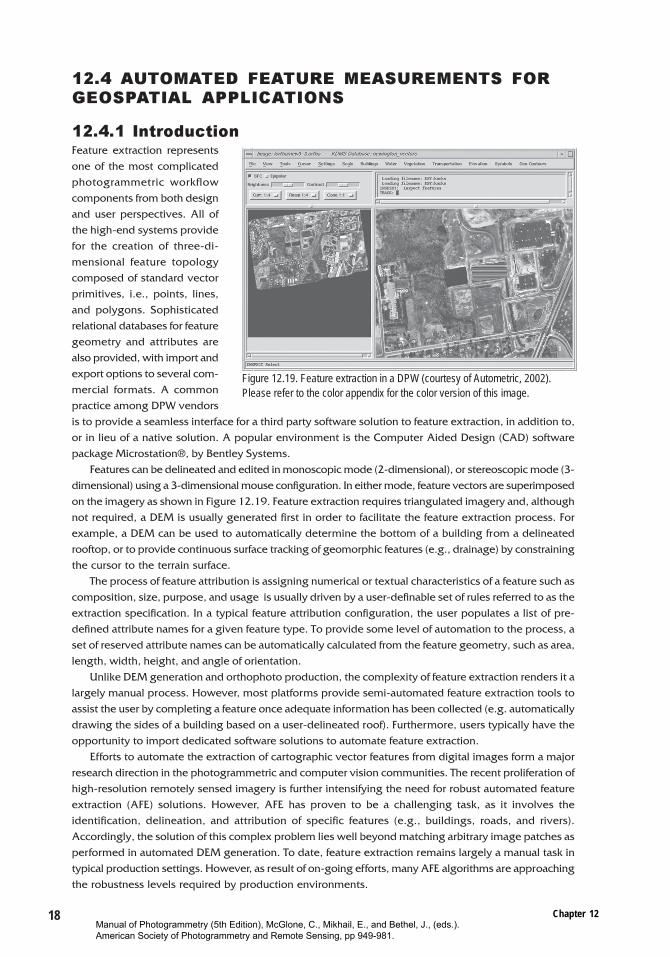
12.4.1 IntroductionFeature extraction representsone of the most complicatedphotogrammetric workflowcomponents from both designand user perspectives. All ofthe high-end systems providefor the creation of three-di-mensional feature topologycomposed of standard vectorprimitives, i.e., points, lines,and polygons. Sophisticatedrelational databases for featuregeometry and attributes arealso provided, with import andexport options to several com-mercial formats. A commonpractice among DPW vendorsis to provide a seamless interface for a third party software solution to feature extraction, in addition to,or in lieu of a native solution. A popular environment is the Computer Aided Design (CAD) softwarepackage Microstation®, by Bentley Systems.
Features can be delineated and edited in monoscopic mode (2-dimensional), or stereoscopic mode (3-dimensional) using a 3-dimensional mouse configuration. In either mode, feature vectors are superimposedon the imagery as shown in Figure 12.19. Feature extraction requires triangulated imagery and, althoughnot required, a DEM is usually generated first in order to facilitate the feature extraction process. Forexample, a DEM can be used to automatically determine the bottom of a building from a delineatedrooftop, or to provide continuous surface tracking of geomorphic features (e.g., drainage) by constrainingthe cursor to the terrain surface.
The process of feature attribution is assigning numerical or textual characteristics of a feature such ascomposition, size, purpose, and usage is usually driven by a user-definable set of rules referred to as theextraction specification. In a typical feature attribution configuration, the user populates a list of pre-defined attribute names for a given feature type. To provide some level of automation to the process, aset of reserved attribute names can be automatically calculated from the feature geometry, such as area,length, width, height, and angle of orientation.
Unlike DEM generation and orthophoto production, the complexity of feature extraction renders it alargely manual process. However, most platforms provide semi-automated feature extraction tools toassist the user by completing a feature once adequate information has been collected (e.g. automaticallydrawing the sides of a building based on a user-delineated roof). Furthermore, users typically have theopportunity to import dedicated software solutions to automate feature extraction.
Efforts to automate the extraction of cartographic vector features from digital images form a majorresearch direction in the photogrammetric and computer vision communities. The recent proliferation ofhigh-resolution remotely sensed imagery is further intensifying the need for robust automated featureextraction (AFE) solutions. However, AFE has proven to be a challenging task, as it involves theidentification, delineation, and attribution of specific features (e.g., buildings, roads, and rivers).Accordingly, the solution of this complex problem lies well beyond matching arbitrary image patches asperformed in automated DEM generation. To date, feature extraction remains largely a manual task intypical production settings. However, as result of on-going efforts, many AFE algorithms are approachingthe robustness levels required by production environments.
Figure 12.19. Feature extraction in a DPW (courtesy of Autometric, 2002).Please refer to the color appendix for the color version of this image.
Manual of Photogrammetry (5th Edition), McGlone, C., Mikhail, E., and Bethel, J., (eds.). American Society of Photogrammetry and Remote Sensing, pp 949-981.
Automation and Digital Photogrammetric Workstations 19
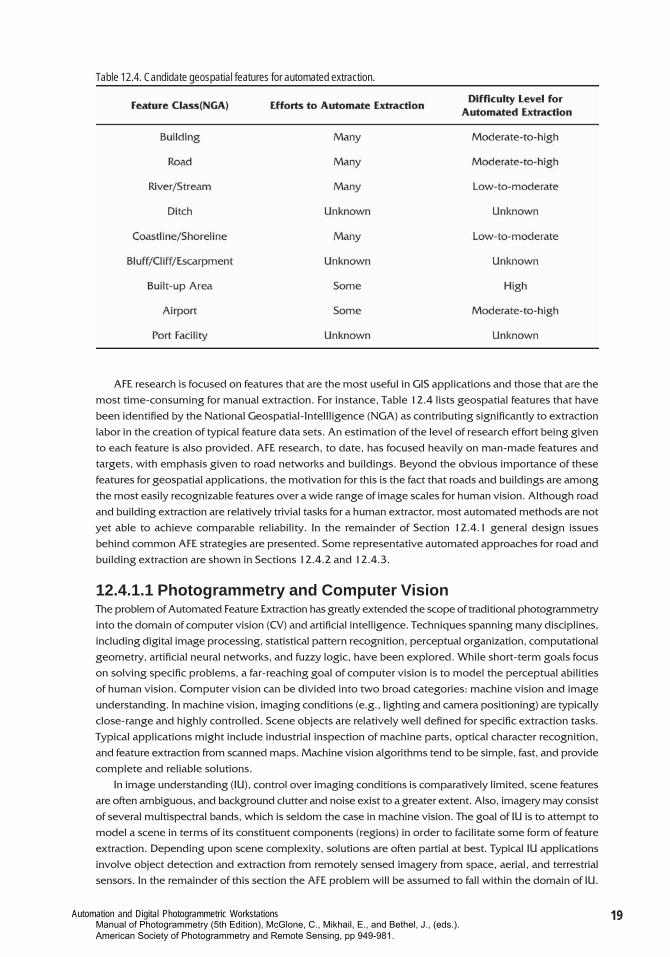
AFE research is focused on features that are the most useful in GIS applications and those that are themost time-consuming for manual extraction. For instance, Table 12.4 lists geospatial features that havebeen identified by the National Geospatial-Intellligence (NGA) as contributing significantly to extractionlabor in the creation of typical feature data sets. An estimation of the level of research effort being givento each feature is also provided. AFE research, to date, has focused heavily on man-made features andtargets, with emphasis given to road networks and buildings. Beyond the obvious importance of thesefeatures for geospatial applications, the motivation for this is the fact that roads and buildings are amongthe most easily recognizable features over a wide range of image scales for human vision. Although roadand building extraction are relatively trivial tasks for a human extractor, most automated methods are notyet able to achieve comparable reliability. In the remainder of Section 12.4.1 general design issuesbehind common AFE strategies are presented. Some representative automated approaches for road andbuilding extraction are shown in Sections 12.4.2 and 12.4.3.
12.4.1.1 Photogrammetry and Computer VisionThe problem of Automated Feature Extraction has greatly extended the scope of traditional photogrammetryinto the domain of computer vision (CV) and artificial intelligence. Techniques spanning many disciplines,including digital image processing, statistical pattern recognition, perceptual organization, computationalgeometry, artificial neural networks, and fuzzy logic, have been explored. While short-term goals focuson solving specific problems, a far-reaching goal of computer vision is to model the perceptual abilitiesof human vision. Computer vision can be divided into two broad categories: machine vision and imageunderstanding. In machine vision, imaging conditions (e.g., lighting and camera positioning) are typicallyclose-range and highly controlled. Scene objects are relatively well defined for specific extraction tasks.Typical applications might include industrial inspection of machine parts, optical character recognition,and feature extraction from scanned maps. Machine vision algorithms tend to be simple, fast, and providecomplete and reliable solutions.
In image understanding (IU), control over imaging conditions is comparatively limited, scene featuresare often ambiguous, and background clutter and noise exist to a greater extent. Also, imagery may consistof several multispectral bands, which is seldom the case in machine vision. The goal of IU is to attempt tomodel a scene in terms of its constituent components (regions) in order to facilitate some form of featureextraction. Depending upon scene complexity, solutions are often partial at best. Typical IU applicationsinvolve object detection and extraction from remotely sensed imagery from space, aerial, and terrestrialsensors. In the remainder of this section the AFE problem will be assumed to fall within the domain of IU.
Table 12.4. Candidate geospatial features for automated extraction.
Manual of Photogrammetry (5th Edition), McGlone, C., Mikhail, E., and Bethel, J., (eds.). American Society of Photogrammetry and Remote Sensing, pp 949-981.
20 Chapter 12
12.4.1.2 Feature Detection versus DelineationAutomated Feature Extraction commonly refers to a class of CV algorithms that address the tasks offeature detection and feature delineation. Feature detection represents a scene segmentation process inwhich image pixels are associated with specific feature patterns based on spatial and/or radiometricproperties. Pixel-feature associations are generally made with Type I operators, examples of whichinclude edge detection, spectral classification, histogram thresholding, texture analysis, and correlationmatching. Type I operators are useful in applications such as automated target recognition, templatematching, and thematic classification of scene regions.
In feature delineation, features are collected and displayed as vectors in a complete and precisetopological representation suitable for subsequent GIS analysis and database storage. Such representationsusually assume the form of strings of connected pixels, or preferably, points, lines or polygon vectors.Feature delineation is performed with Type II operators, which include methods for linking and groupingpixels into larger feature components. Type II operators usually work in conjunction with Type I operatorsin that the output of the latter serves as input to the former. Omission and commission errors generatedfrom Type I output are minimized to some extent by Type II operators. For example, feature gaps(omission errors) are filled in, and clutter (commission error) is ignored. Examples of Type II operatorsinclude region growing, the Hough transform, and line trackers.
As scene structure increases in complexity, so does the need for more sophisticated AFE techniques.Urban scenes generally present more structural complexity than rural scenes. For instance, automateddelineation of roads in urban scenes is complicated by road markings, vehicular traffic, parking lots,driveways, sidewalks, curbs, and shadows. By contrast, extraction of a radiometrically homogeneousroad going through a desert is a comparatively trivial task for a simple AFE technique.
12.4.1.3 Degrees of AutomationAutomated feature extraction strategies are often categorized according to their degree of automationinto semi- or fully automatic. The objective of semi-automatic methods is to assist the human operator inreal-time. This strategy is designed to use interactive user-provided information in the form of seedpoints, widths, and directions, with real-time manual editing of the extraction results. On the other hand,real-time execution sets limits on the computational complexity of the algorithm.
A fully automatic extraction strategy is intended to extract features from a scene as an offlineprocess, i.e., without the need of user-provided inputs. This is often suitable to perform GIS updates, inwhich existing coarse or outdated feature data is used to guide a revised extraction. A successful updateis dependent upon the accuracy of the reference data relative to the extraction image. A feature updatestrategy is an example of a top-down process in that it begins with a priori reference information to guidefeature extraction. Given current worldwide feature database holdings, an update strategy offers apractical approach to revise and refine existing data. However, for extraction of new features, a rigorousapproach to full automation is needed in the sense that there can be no reliance on reference vector data.A rigorous strategy is also motivated by gaining insight into the nature of the extraction problem as avision process. A standard methodology begins with low-level detection that generates initial hypothesesfor candidate feature components, followed by mid-level grouping of components, and concludes withhigh-level reasoning for feature completion. This operational flow is an example of a bottom up, or data-driven process.
12.4.1.4 General StrategiesAutomated feature extraction techniques often use a toolbox approach, in which a collection of specializedfeature models is assembled in a single algorithm to accommodate variable scene content. Regardless ofthe algorithm, three key strategies are often used to support feature extraction 1) using scale space, 2)using context in scene interpretation, and 3) data fusion. A synopsis of each strategy follows.
Scale space. Several photogrammetric processes make use of image pyramids, also known as reducedresolution data sets. Image pyramids are an example of scale space [Koenderink, 1984; Witkin, 1983]. Incomputer vision, image scale space is used to extract the manifestations of features at dif ferent image
Manual of Photogrammetry (5th Edition), McGlone, C., Mikhail, E., and Bethel, J., (eds.). American Society of Photogrammetry and Remote Sensing, pp 949-981.
Automation and Digital Photogrammetric Workstations 21
scales. For example, the use of image scale space can optimize the extraction of salient features by firstisolating them at lower resolutions, and then homing in on their precise locations at higher resolutions.In this way, extraction at lower resolutions serves to initialize subsequent extractions at higher resolutions.There is ample evidence to suggest that scale space processing is inherent in human vision.
Scene context. Modeling scene context is motivated by perceptual organization in human vision. Thepremise is to interpret and exploit background scene components more completely to provide a contextualreference that enhances the extraction of target features, as opposed to a more constrained approach thatonly distinguishes targets from non-targets. For example, road markings and vehicular traffic can providevaluable cues for the existence of roads. Modeling scene context generally increases the complexity ofthe algorithm.
Data fusion. The goal of data fusion is to merge different types of information to enhance therecognition of features. High-resolution multispectral and hyperspectral imagery and high-resolutionDEMs have become very useful information sources for automated extraction algorithms. The premise isthat solution robustness can be increased when several different input sources of information areanalyzed. However, the increase in computational complexity sets an upper limit on the effectiveness ofdata fusion.
12.4.1.5 Evaluating the Performance of Extraction AlgorithmsThe development of a variety of algorithms to support AFE has brought attention to the development ofrobust performance evaluation metrics for these techniques [Bowyer and Phillips, 1998; McKeown et al.,2000]. Practical utility of an algorithm within a production environment is ultimately determined by itsusage cost. An algorithm’s usage cost includes algorithm initialization (e.g. selection of seed points anddefinition of algorithm parameters), algorithm execution (computer run time), and the subsequent manualediting of its output to meet accuracy requirements. Usage cost is typically expressed as a comparison(e.g. fraction) of the level of effort expended in algorithm-based extraction versus completely manualextraction for the same job.
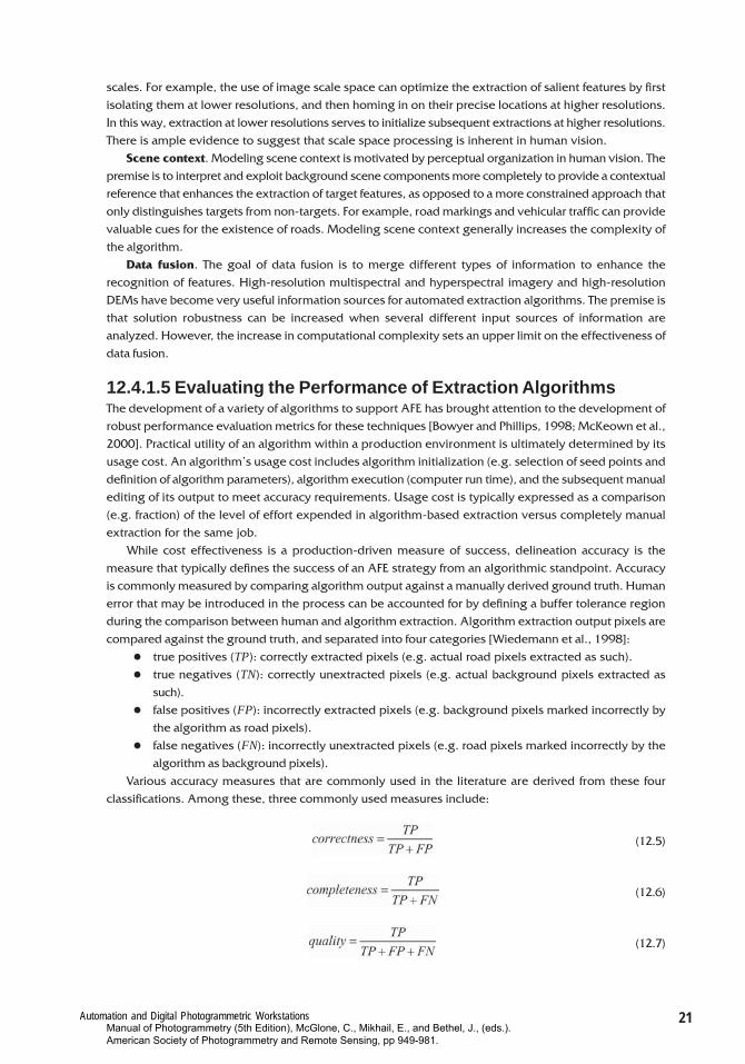
While cost effectiveness is a production-driven measure of success, delineation accuracy is themeasure that typically defines the success of an AFE strategy from an algorithmic standpoint. Accuracyis commonly measured by comparing algorithm output against a manually derived ground truth. Humanerror that may be introduced in the process can be accounted for by defining a buffer tolerance regionduring the comparison between human and algorithm extraction. Algorithm extraction output pixels arecompared against the ground truth, and separated into four categories [Wiedemann et al., 1998]:
� true positives (TP): correctly extracted pixels (e.g. actual road pixels extracted as such).� true negatives (TN): correctly unextracted pixels (e.g. actual background pixels extracted as
such).� false positives (FP): incorrectly extracted pixels (e.g. background pixels marked incorrectly by
the algorithm as road pixels).� false negatives (FN): incorrectly unextracted pixels (e.g. road pixels marked incorrectly by the
algorithm as background pixels).Various accuracy measures that are commonly used in the literature are derived from these four
classifications. Among these, three commonly used measures include:
(12.5)
(12.6)
(12.7)
Manual of Photogrammetry (5th Edition), McGlone, C., Mikhail, E., and Bethel, J., (eds.). American Society of Photogrammetry and Remote Sensing, pp 949-981.
22 Chapter 12
Correctness is a measure ranging between 0 and 1 that indicates the detection accuracy rate relativeto ground truth. It can also be interpreted as the converse of commission error, such that correctness +
commission_error = 1. Completeness is also a measure ranging between 0 and 1 that can be interpretedas the converse of omission error, such that completeness + omission_error = 1. Completeness andcorrectness are complementary metrics that clearly need to be interpreted simultaneously. For example,if all scene pixels are classified as TPs, then the completeness value is a perfect 1.0; of course thecorrectness value would likely be near 0. A more meaningful single metric is quality, which is a normalizedmeasure between correctness and completeness.The quality value can never be higher than either thecompleteness or correctness.
12.4.2 Automating Road ExtractionSince a road network does not conform to a specific global shape, the detection process must begin byconsidering local shape characteristics. Road extraction algorithms commonly use geometric andradiometric attributes to model the appearance of a road segment. With respect to geometry, roads aregenerally considered to be elongated, constant in width, linear to mildly curvilinear, smoothly curved,continuous, and connected into networks. In low-resolution images roads are single-pixel-width lines,whereas in high-resolution images roads are characterized geometrically as the area within a pair ofedges. With respect to radiometry, road models tend to assume good contrast, well-defined and connectedgradients, homogeneity, and smooth texture. As many road models are based on gradient and textureanalysis of high-resolution imagery, input images are often single-layer (e.g., panchromatic). However,models that incorporate spectral analysis can exploit the content of multispectral images [Agouris et al.,2002].
Initially most approaches to road extraction focused on scenes with mainly rural content as they aremuch less complex and easier to model than urban scenes. However, in recent years researchers havedeveloped models for urban scene content for road extraction. Approaches to urban scenes includemodeling road markings (which require a spatial resolution of about 0.2-0.5m per pixel) [Baumgartner etal., 1999b], or exploiting the geometric regularity of city grids [Price, 2000].
Over the last two decades, a few prominent modeling techniques have emerged from road extractionresearch. Among them, tracking, anti-parallel edge detection, and snakes are representative of a progresstowards more complex road models. In the remainder of this section a brief overview of these techniquesis provided, and the section concludes with examples from recently developed road extraction strategiesthat employ these techniques.
12.4.2.1 Interactive Road TrackingRoad tracking or following is a local exploratory technique within a scene. In interactive tracking, theprocess is user-initialized in real time with a starting point, start direction, and/or feature width. Thealgorithm then predicts the trajectory of the road in incremental steps until it reaches a stoppingcriterion. One technique for prediction is to fit a polynomial such as a parabola to the most recentlyidentified path points [McKeown and Denlinger, 1988]. The tracking process may combine edge, radiometricand/or textural constraints via template/correlation matching, whose patterns are derived from thestarting point, and periodically updated to better model local conditions along the road path.
More robust algorithms allow for gradual surface and width changes along a track, as well as negotiatingocclusions such as shadows, vehicles, surface markings, and surface irregularities. Additional searchparameters often include a search radius, allowable gap size, search angle, junction options, curvaturerate, and line smoothing and generalization. An effective approach to the problem is to provide an on-the-fly input mode in which the algorithm stops when it encounters potential obstacles such as overpassesand intersections, and prompts the user to determine how the algorithm should proceed.
12.4.2.2 Road Detection from the Anti-Parallel Edge ModelOver the last two decades, gradient analysis has perhaps provided the most motivation for road extractionalgorithms. A simple and well-known technique for detecting roads in high-resolution images is via anti-
Manual of Photogrammetry (5th Edition), McGlone, C., Mikhail, E., and Bethel, J., (eds.). American Society of Photogrammetry and Remote Sensing, pp 949-981.
Automation and Digital Photogrammetric Workstations 23
parallel (apar) edge detection [Nevatia and Ramesh, 1980; Zlotnick and Carnine, 1993]. Given its prominencein the literature, the apar method is presented in some detail to provide an indication of the practicalutility and limitations of automated road detection.
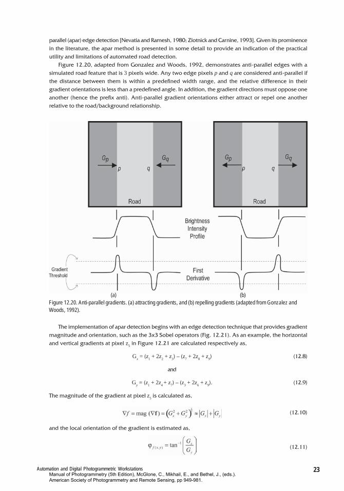
Figure 12.20, adapted from Gonzalez and Woods, 1992, demonstrates anti-parallel edges with asimulated road feature that is 3 pixels wide. Any two edge pixels p and q are considered anti-parallel ifthe distance between them is within a predefined width range, and the relative difference in theirgradient orientations is less than a predefined angle. In addition, the gradient directions must oppose oneanother (hence the prefix anti). Anti-parallel gradient orientations either attract or repel one anotherrelative to the road/background relationship.
The implementation of apar detection begins with an edge detection technique that provides gradientmagnitude and orientation, such as the 3x3 Sobel operators (Fig. 12.21). As an example, the horizontaland vertical gradients at pixel z5 in Figure 12.21 are calculated respectively as,
Gx = (z1 + 2z2 + z3) – (z7 + 2z8 + z9) (12.8)
and
Gy = (z1 + 2z4 + z7) – (z3 + 2z6 + z9). (12.9)
The magnitude of the gradient at pixel z5 is calculated as,
(12.10)
and the local orientation of the gradient is estimated as,
(12.11)
(a) (b)Figure 12.20. Anti-parallel gradients. (a) attracting gradients, and (b) repelling gradients (adapted from Gonzalez andWoods, 1992).
Manual of Photogrammetry (5th Edition), McGlone, C., Mikhail, E., and Bethel, J., (eds.). American Society of Photogrammetry and Remote Sensing, pp 949-981.
24 Chapter 12
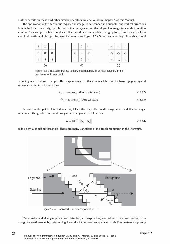
Further details on these and other similar operators may be found in Chapter 5 of this Manual.The application of this technique requires an image to be scanned in horizontal and vertical directions
in search of successive edge pixels p and q that satisfy road width and gradient magnitude and orientationcriteria. For example, a horizontal scan line first detects a candidate edge pixel p, and searches for acandidate anti-parallel edge pixel q on the same row (Figure 12.22). Vertical scanning follows horizontal
scanning, and results are merged. The perpendicular width estimate of the road for two edge pixels p andq on a scan line is determined as,
(Horizontal scan) (12.12)
(Vertical scan) (12.13)
An anti-parallel pair is detected when w pq
falls within a specified width range, and the deflection angleα between the gradient orientations gradients at p and q, defined as
(12.14)
falls below a specified threshold. There are many variations of this implementation in the literature.
Once anti-parallel edge pixels are detected, corresponding centerline pixels are derived in astraightforward manner by determining the midpoint between anti-parallel pixels. Road network topology
(c)(b)(a)
Figure 12.21. 3x3 Sobel masks. (a) horizontal detector, (b) vertical detector, and (c)gray levels of image patch.
Figure 12.22. Horizontal scan for anti-parallel pixels.
Manual of Photogrammetry (5th Edition), McGlone, C., Mikhail, E., and Bethel, J., (eds.). American Society of Photogrammetry and Remote Sensing, pp 949-981.
Automation and Digital Photogrammetric Workstations 25
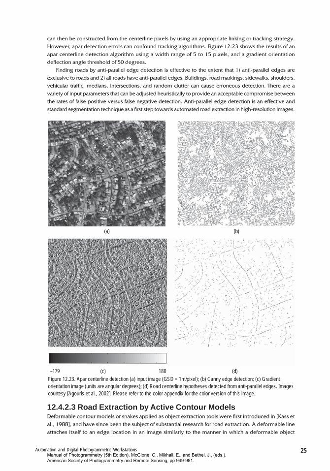
can then be constructed from the centerline pixels by using an appropriate linking or tracking strategy.However, apar detection errors can confound tracking algorithms. Figure 12.23 shows the results of anapar centerline detection algorithm using a width range of 5 to 15 pixels, and a gradient orientationdeflection angle threshold of 50 degrees.
Finding roads by anti-parallel edge detection is effective to the extent that 1) anti-parallel edges areexclusive to roads and 2) all roads have anti-parallel edges. Buildings, road markings, sidewalks, shoulders,vehicular traffic, medians, intersections, and random clutter can cause erroneous detection. There are avariety of input parameters that can be adjusted heuristically to provide an acceptable compromise betweenthe rates of false positive versus false negative detection. Anti-parallel edge detection is an effective andstandard segmentation technique as a first step towards automated road extraction in high-resolution images.
12.4.2.3 Road Extraction by Active Contour ModelsDeformable contour models or snakes applied as object extraction tools were first introduced in [Kass etal., 1988], and have since been the subject of substantial research for road extraction. A deformable lineattaches itself to an edge location in an image similarly to the manner in which a deformable object
(a) (b)
–179 (c) 180 (d)Figure 12.23. Apar centerline detection (a) input image (GSD = 1m/pixel); (b) Canny edge detection; (c) Gradientorientation image (units are angular degrees); (d) Road centerline hypotheses detected from anti-parallel edges. Imagescourtesy [Agouris et al., 2002]. Please refer to the color appendix for the color version of this image.
Manual of Photogrammetry (5th Edition), McGlone, C., Mikhail, E., and Bethel, J., (eds.). American Society of Photogrammetry and Remote Sensing, pp 949-981.
26 Chapter 12
embedded in a viscous medium deforms its shape until it reaches a stage of stability. In its numericalsolution the snake is represented by a polygonal line (i.e., nodes connected by segments). The geometricand radiometric relations of these nodes are expressed as energy functions, and object extractionbecomes an optimization problem. The main issues are how to define the energy at the snake nodes andhow to solve the energy minimization problem.
In general, the energy function of a snake contains internal and external forces. The internal forcesregulate the ability of the contour to stretch or bend at a specific point. The external force attracts thecontour to image features (e.g., edges). Additionally, external constraints may be used to express user-imposed restrictions (e.g., to force the snake to pass through specific points).The total energy of each point is expressed as
(12.15)
where,� Econt , Ecurv are expressions of the first and second order continuity constraints (internal forces),� Eedge is an expression of the edge strength (external force), and� α, β, and γ are relative weights describing the importance of each energy term.
A brief description of these energy functions follows [Agouris, et al., 2001].Continuity term: If v i = (x
i, y
i) is a point on the contour, the first energy term in (12.15) is defined as:
(12.16)
where d is the average distance between the n points:
(12.17)
The continuity component forces snake nodes to be evenly spaced, avoiding grouping at certain areas,while at the same time minimizing the distance between them.
Curvature term: This term expresses the curvature of the snake contour, and allows for the manipulationof its flexibility and appearance:
(12.18)
Edge term: Continuity and curvature describe the geometry of the contour and are referred to asinternal forces of the snake. The third term describes the relation of the contour to the radiometriccontent of the image, and is referred to as external force. In general, it forces points to move towardsimage edges. An expression of such a force may be defined as
(12.19)
The above model attracts the snake to image points with high gradient values. Since the gradient isa metric for the edges of an image, the snake is attracted to strong edge points. The gradient of the imageat each point is normalized to display small differences in values at the neighborhood of that point.
The coefficients α, β, and γ in (12.15) are weights describing the relative importance of each energyterm in the solution. Increasing the relative values of α and β will result in putting more emphasis on thegeometric smoothness of the extracted line. This might be suitable for very noisy images, but might beunsuitable when dealing with sharp angles in the object space. Increasing the relative value of γ placesmore emphasis on the radiometric content of the image, regardless of the physical appearance of theextracted outline. As is commonly the case in snake solutions, the selection of these parameters isperformed empirically.
Together, the three energy functions describe an ideal model of a road segment, namely a smoothcurve coinciding with a strong edge in the image. The objective of traditional snake-based road extractionis to identify in an image a sequence of points describing a contour that approximates this ideal model.
Manual of Photogrammetry (5th Edition), McGlone, C., Mikhail, E., and Bethel, J., (eds.). American Society of Photogrammetry and Remote Sensing, pp 949-981.
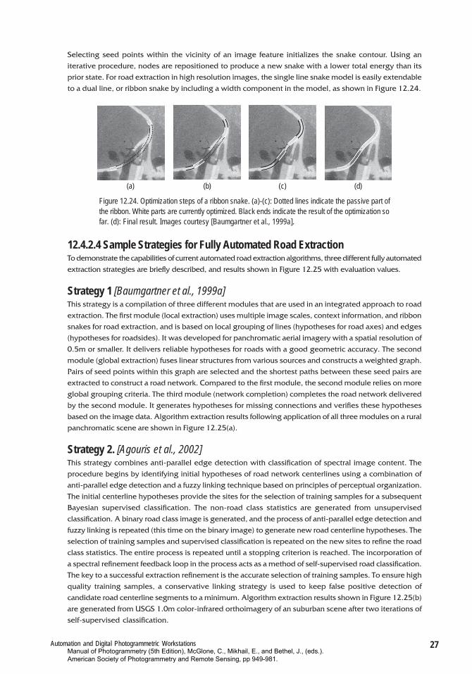
Automation and Digital Photogrammetric Workstations 27
Selecting seed points within the vicinity of an image feature initializes the snake contour. Using aniterative procedure, nodes are repositioned to produce a new snake with a lower total energy than itsprior state. For road extraction in high resolution images, the single line snake model is easily extendableto a dual line, or ribbon snake by including a width component in the model, as shown in Figure 12.24.
12.4.2.4 Sample Strategies for Fully Automated Road ExtractionTo demonstrate the capabilities of current automated road extraction algorithms, three different fully automatedextraction strategies are briefly described, and results shown in Figure 12.25 with evaluation values.
Strategy 1 [Baumgartner et al., 1999a]This strategy is a compilation of three different modules that are used in an integrated approach to roadextraction. The first module (local extraction) uses multiple image scales, context information, and ribbonsnakes for road extraction, and is based on local grouping of lines (hypotheses for road axes) and edges(hypotheses for roadsides). It was developed for panchromatic aerial imagery with a spatial resolution of0.5m or smaller. It delivers reliable hypotheses for roads with a good geometric accuracy. The secondmodule (global extraction) fuses linear structures from various sources and constructs a weighted graph.Pairs of seed points within this graph are selected and the shortest paths between these seed pairs areextracted to construct a road network. Compared to the first module, the second module relies on moreglobal grouping criteria. The third module (network completion) completes the road network deliveredby the second module. It generates hypotheses for missing connections and verifies these hypothesesbased on the image data. Algorithm extraction results following application of all three modules on a ruralpanchromatic scene are shown in Figure 12.25(a).
Strategy 2. [Agouris et al., 2002]This strategy combines anti-parallel edge detection with classification of spectral image content. Theprocedure begins by identifying initial hypotheses of road network centerlines using a combination ofanti-parallel edge detection and a fuzzy linking technique based on principles of perceptual organization.The initial centerline hypotheses provide the sites for the selection of training samples for a subsequentBayesian supervised classification. The non-road class statistics are generated from unsupervisedclassification. A binary road class image is generated, and the process of anti-parallel edge detection andfuzzy linking is repeated (this time on the binary image) to generate new road centerline hypotheses. Theselection of training samples and supervised classification is repeated on the new sites to refine the roadclass statistics. The entire process is repeated until a stopping criterion is reached. The incorporation ofa spectral refinement feedback loop in the process acts as a method of self-supervised road classification.The key to a successful extraction refinement is the accurate selection of training samples. To ensure highquality training samples, a conservative linking strategy is used to keep false positive detection ofcandidate road centerline segments to a minimum. Algorithm extraction results shown in Figure 12.25(b)are generated from USGS 1.0m color-infrared orthoimagery of an suburban scene after two iterations ofself-supervised classification.
(a) (b) (c) (d)
Figure 12.24. Optimization steps of a ribbon snake. (a)-(c): Dotted lines indicate the passive part ofthe ribbon. White parts are currently optimized. Black ends indicate the result of the optimization sofar. (d): Final result. Images courtesy [Baumgartner et al., 1999a].
Manual of Photogrammetry (5th Edition), McGlone, C., Mikhail, E., and Bethel, J., (eds.). American Society of Photogrammetry and Remote Sensing, pp 949-981.
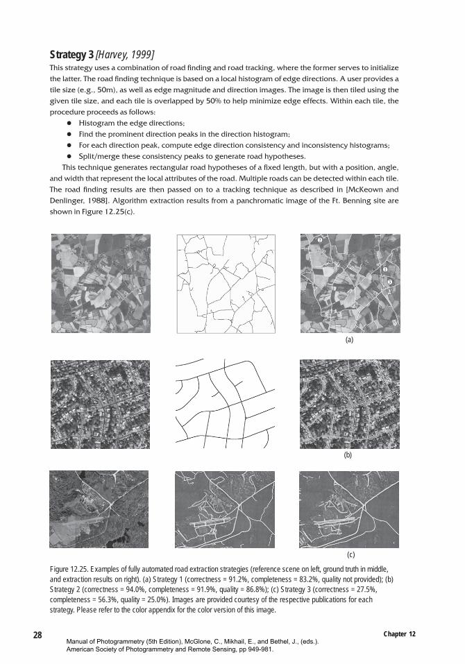
28 Chapter 12
Strategy 3 [Harvey, 1999]This strategy uses a combination of road finding and road tracking, where the former serves to initializethe latter. The road finding technique is based on a local histogram of edge directions. A user provides atile size (e.g., 50m), as well as edge magnitude and direction images. The image is then tiled using thegiven tile size, and each tile is overlapped by 50% to help minimize edge effects. Within each tile, theprocedure proceeds as follows:
� Histogram the edge directions;� Find the prominent direction peaks in the direction histogram;� For each direction peak, compute edge direction consistency and inconsistency histograms;� Split/merge these consistency peaks to generate road hypotheses.
This technique generates rectangular road hypotheses of a fixed length, but with a position, angle,and width that represent the local attributes of the road. Multiple roads can be detected within each tile.The road finding results are then passed on to a tracking technique as described in [McKeown andDenlinger, 1988]. Algorithm extraction results from a panchromatic image of the Ft. Benning site areshown in Figure 12.25(c).
Figure 12.25. Examples of fully automated road extraction strategies (reference scene on left, ground truth in middle,and extraction results on right). (a) Strategy 1 (correctness = 91.2%, completeness = 83.2%, quality not provided); (b)Strategy 2 (correctness = 94.0%, completeness = 91.9%, quality = 86.8%); (c) Strategy 3 (correctness = 27.5%,completeness = 56.3%, quality = 25.0%). Images are provided courtesy of the respective publications for eachstrategy. Please refer to the color appendix for the color version of this image.
(a)
(b)
(c)
Manual of Photogrammetry (5th Edition), McGlone, C., Mikhail, E., and Bethel, J., (eds.). American Society of Photogrammetry and Remote Sensing, pp 949-981.
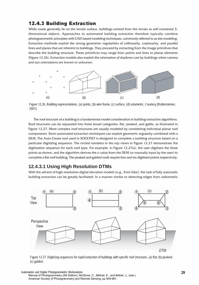
Automation and Digital Photogrammetric Workstations 29
12.4.3 Building ExtractionWhile roads generally lie on the terrain surface, buildings extend from the terrain as self-contained 3-dimensional objects. Approaches to automated building extraction therefore typically combinephotogrammetric principles with CAD-based modeling techniques, commonly referred to as site modeling.Extraction methods exploit the strong geometric regularities of collinearity, coplanarity, and parallellines and planes that are inherent to buildings. They proceed by extracting from the image primitives thatdescribe the building structure. These primitives may range from points and lines to planar elements(Figure 12.26). Extraction models also exploit the orientation of shadows cast by buildings when cameraand sun orientations are known or unknown.
The roof structure of a building is a fundamental model consideration in building extraction algorithms.Roof structures can be separated into three broad categories: flat, peaked, and gable, as illustrated inFigure 12.27. More complex roof structures are usually modeled by considering individual planar roofcomponents. Semi-automated extraction techniques can exploit geometric regularity combined with aDEM. The Auto Create tool used in SOCETSET is designed to complete a building structure based on aparticular digitizing sequence. The circled numbers in the top views in Figure 12.27 demonstrate thedigitization sequence for each roof type. For example, in Figure 12.27(a), the user digitizes the threepoints as shown, and the algorithm derives the z-value from the DEM (or manually input by the user) tocomplete a flat roof building. The peaked and gabled roofs require four and six digitized points respectively.
12.4.3.1 Using High Resolution DTMsWith the advent of high-resolution digital elevation models (e.g., from lidar), the task of fully automaticbuilding extraction can be greatly facilitated. In a manner similar to detecting edges from radiometric
(a) (b) (c) (d)
Figure 12.26. Building representations. (a) points, (b) wire frame, (c) surface, (d) volumetric. Courtesy [Rottensteiner,2001].
Figure 12.27. Digitizing sequences for rapid extraction of buildings with specific roof structures. (a) flat; (b) peaked;(c) gabled.
Manual of Photogrammetry (5th Edition), McGlone, C., Mikhail, E., and Bethel, J., (eds.). American Society of Photogrammetry and Remote Sensing, pp 949-981.
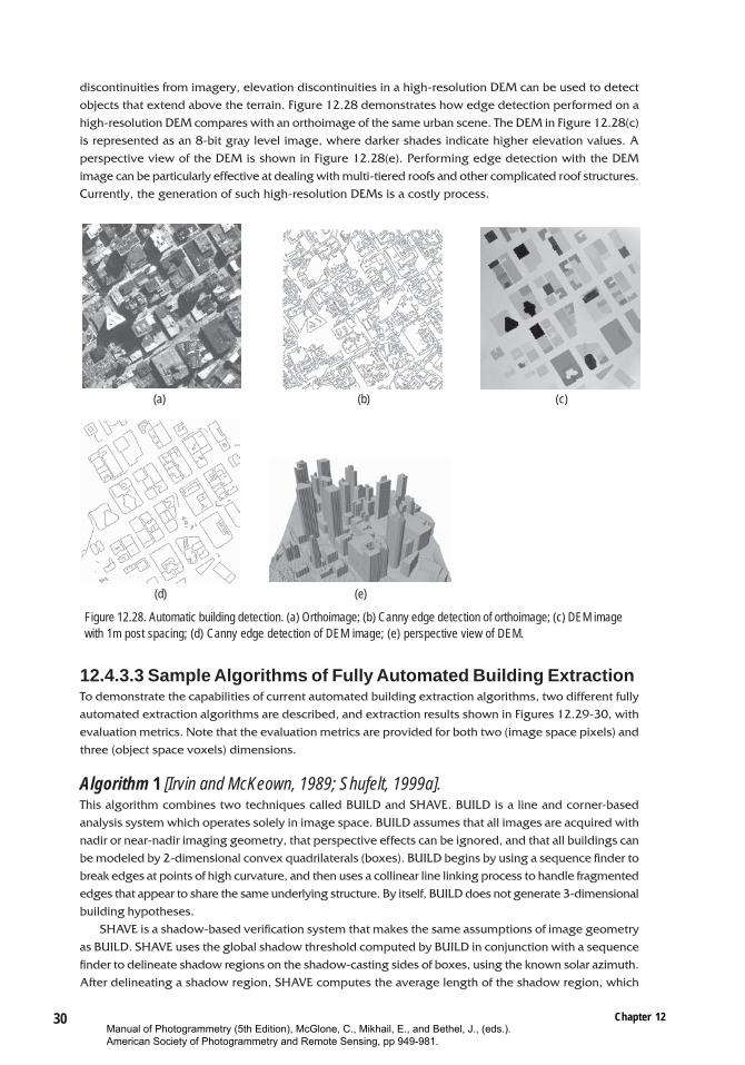
30 Chapter 12
discontinuities from imagery, elevation discontinuities in a high-resolution DEM can be used to detectobjects that extend above the terrain. Figure 12.28 demonstrates how edge detection performed on ahigh-resolution DEM compares with an orthoimage of the same urban scene. The DEM in Figure 12.28(c)is represented as an 8-bit gray level image, where darker shades indicate higher elevation values. Aperspective view of the DEM is shown in Figure 12.28(e). Performing edge detection with the DEMimage can be particularly effective at dealing with multi-tiered roofs and other complicated roof structures.Currently, the generation of such high-resolution DEMs is a costly process.
12.4.3.3 Sample Algorithms of Fully Automated Building ExtractionTo demonstrate the capabilities of current automated building extraction algorithms, two different fullyautomated extraction algorithms are described, and extraction results shown in Figures 12.29-30, withevaluation metrics. Note that the evaluation metrics are provided for both two (image space pixels) andthree (object space voxels) dimensions.
Algorithm 1 [Irvin and McKeown, 1989; Shufelt, 1999a].This algorithm combines two techniques called BUILD and SHAVE. BUILD is a line and corner-basedanalysis system which operates solely in image space. BUILD assumes that all images are acquired withnadir or near-nadir imaging geometry, that perspective effects can be ignored, and that all buildings canbe modeled by 2-dimensional convex quadrilaterals (boxes). BUILD begins by using a sequence finder tobreak edges at points of high curvature, and then uses a collinear line linking process to handle fragmentededges that appear to share the same underlying structure. By itself, BUILD does not generate 3-dimensionalbuilding hypotheses.
SHAVE is a shadow-based verification system that makes the same assumptions of image geometryas BUILD. SHAVE uses the global shadow threshold computed by BUILD in conjunction with a sequencefinder to delineate shadow regions on the shadow-casting sides of boxes, using the known solar azimuth.After delineating a shadow region, SHAVE computes the average length of the shadow region, which
(a) (b) (c)
(d) (e)
Figure 12.28. Automatic building detection. (a) Orthoimage; (b) Canny edge detection of orthoimage; (c) DEM imagewith 1m post spacing; (d) Canny edge detection of DEM image; (e) perspective view of DEM.
Manual of Photogrammetry (5th Edition), McGlone, C., Mikhail, E., and Bethel, J., (eds.). American Society of Photogrammetry and Remote Sensing, pp 949-981.
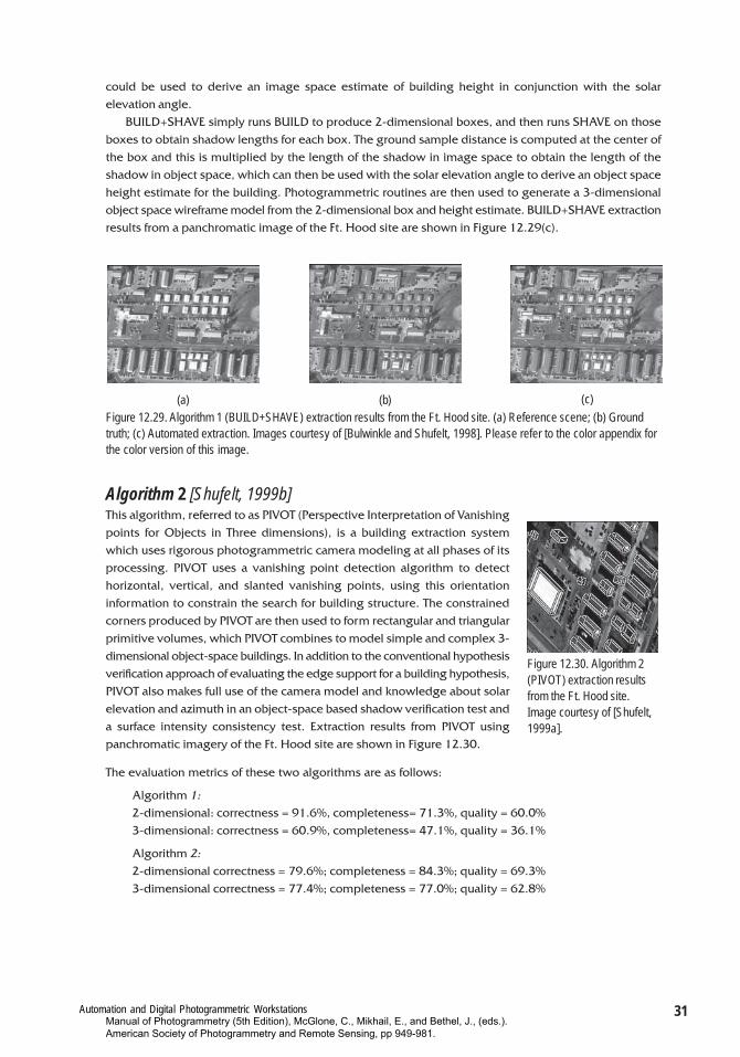
Automation and Digital Photogrammetric Workstations 31
could be used to derive an image space estimate of building height in conjunction with the solarelevation angle.
BUILD+SHAVE simply runs BUILD to produce 2-dimensional boxes, and then runs SHAVE on thoseboxes to obtain shadow lengths for each box. The ground sample distance is computed at the center ofthe box and this is multiplied by the length of the shadow in image space to obtain the length of theshadow in object space, which can then be used with the solar elevation angle to derive an object spaceheight estimate for the building. Photogrammetric routines are then used to generate a 3-dimensionalobject space wireframe model from the 2-dimensional box and height estimate. BUILD+SHAVE extractionresults from a panchromatic image of the Ft. Hood site are shown in Figure 12.29(c).
Algorithm 2 [Shufelt, 1999b]This algorithm, referred to as PIVOT (Perspective Interpretation of Vanishingpoints for Objects in Three dimensions), is a building extraction systemwhich uses rigorous photogrammetric camera modeling at all phases of itsprocessing. PIVOT uses a vanishing point detection algorithm to detecthorizontal, vertical, and slanted vanishing points, using this orientationinformation to constrain the search for building structure. The constrainedcorners produced by PIVOT are then used to form rectangular and triangularprimitive volumes, which PIVOT combines to model simple and complex 3-dimensional object-space buildings. In addition to the conventional hypothesisverification approach of evaluating the edge support for a building hypothesis,PIVOT also makes full use of the camera model and knowledge about solarelevation and azimuth in an object-space based shadow verification test anda surface intensity consistency test. Extraction results from PIVOT usingpanchromatic imagery of the Ft. Hood site are shown in Figure 12.30.
The evaluation metrics of these two algorithms are as follows:
Algorithm 1:2-dimensional: correctness = 91.6%, completeness= 71.3%, quality = 60.0%3-dimensional: correctness = 60.9%, completeness= 47.1%, quality = 36.1%
Algorithm 2:2-dimensional correctness = 79.6%; completeness = 84.3%; quality = 69.3%3-dimensional correctness = 77.4%; completeness = 77.0%; quality = 62.8%
(a) (b) (c)
Figure 12.29. Algorithm 1 (BUILD+SHAVE) extraction results from the Ft. Hood site. (a) Reference scene; (b) Groundtruth; (c) Automated extraction. Images courtesy of [Bulwinkle and Shufelt, 1998]. Please refer to the color appendix forthe color version of this image.
Figure 12.30. Algorithm 2(PIVOT) extraction resultsfrom the Ft. Hood site.Image courtesy of [Shufelt,1999a].
Manual of Photogrammetry (5th Edition), McGlone, C., Mikhail, E., and Bethel, J., (eds.). American Society of Photogrammetry and Remote Sensing, pp 949-981.
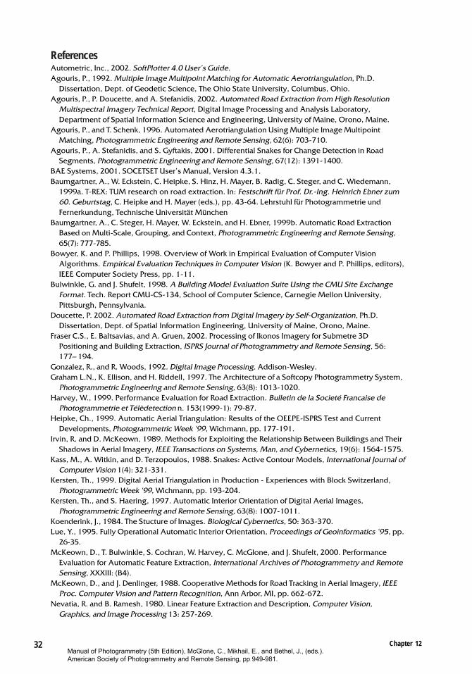
32 Chapter 12
ReferencesAutometric, Inc., 2002. SoftPlotter 4.0 User’s Guide.Agouris, P., 1992. Multiple Image Multipoint Matching for Automatic Aerotriangulation, Ph.D.
Dissertation, Dept. of Geodetic Science, The Ohio State University, Columbus, Ohio.Agouris, P., P. Doucette, and A. Stefanidis, 2002. Automated Road Extraction from High Resolution
Multispectral Imagery Technical Report, Digital Image Processing and Analysis Laboratory,Department of Spatial Information Science and Engineering, University of Maine, Orono, Maine.
Agouris, P., and T. Schenk, 1996. Automated Aerotriangulation Using Multiple Image MultipointMatching, Photogrammetric Engineering and Remote Sensing, 62(6): 703-710.
Agouris, P., A. Stefanidis, and S. Gyftakis, 2001. Differential Snakes for Change Detection in RoadSegments, Photogrammetric Engineering and Remote Sensing, 67(12): 1391-1400.
BAE Systems, 2001. SOCETSET User’s Manual, Version 4.3.1.Baumgartner, A., W. Eckstein, C. Heipke, S. Hinz, H. Mayer, B. Radig, C. Steger, and C. Wiedemann,
1999a. T-REX: TUM research on road extraction. In: Festschrift für Prof. Dr.-Ing. Heinrich Ebner zum60. Geburtstag, C. Heipke and H. Mayer (eds.), pp. 43-64. Lehrstuhl für Photogrammetrie undFernerkundung, Technische Universität München
Baumgartner, A., C. Steger, H. Mayer, W. Eckstein, and H. Ebner, 1999b. Automatic Road ExtractionBased on Multi-Scale, Grouping, and Context, Photogrammetric Engineering and Remote Sensing,65(7): 777-785.
Bowyer, K. and P. Phillips, 1998. Overview of Work in Empirical Evaluation of Computer VisionAlgorithms. Empirical Evaluation Techniques in Computer Vision (K. Bowyer and P. Phillips, editors),IEEE Computer Society Press, pp. 1-11.
Bulwinkle, G. and J. Shufelt, 1998. A Building Model Evaluation Suite Using the CMU Site ExchangeFormat. Tech. Report CMU-CS-134, School of Computer Science, Carnegie Mellon University,Pittsburgh, Pennsylvania.
Doucette, P. 2002. Automated Road Extraction from Digital Imagery by Self-Organization, Ph.D.Dissertation, Dept. of Spatial Information Engineering, University of Maine, Orono, Maine.
Fraser C.S., E. Baltsavias, and A. Gruen, 2002. Processing of Ikonos Imagery for Submetre 3DPositioning and Building Extraction, ISPRS Journal of Photogrammetry and Remote Sensing, 56:177– 194.
Gonzalez, R., and R. Woods, 1992. Digital Image Processing. Addison-Wesley.Graham L.N., K. Ellison, and H. Riddell, 1997. The Architecture of a Softcopy Photogrammetry System,
Photogrammetric Engineering and Remote Sensing, 63(8): 1013-1020.Harvey, W., 1999. Performance Evaluation for Road Extraction. Bulletin de la Societé Francaise de
Photogrammetrie et Télèdetection n. 153(1999-1): 79-87.Heipke, Ch., 1999. Automatic Aerial Triangulation: Results of the OEEPE-ISPRS Test and Current
Developments, Photogrammetric Week ‘99, Wichmann, pp. 177-191.Irvin, R. and D. McKeown, 1989. Methods for Exploiting the Relationship Between Buildings and Their
Shadows in Aerial Imagery, IEEE Transactions on Systems, Man, and Cybernetics, 19(6): 1564-1575.Kass, M., A. Witkin, and D. Terzopoulos, 1988. Snakes: Active Contour Models, International Journal of
Computer Vision 1(4): 321-331.Kersten, Th., 1999. Digital Aerial Triangulation in Production - Experiences with Block Switzerland,
Photogrammetric Week ‘99, Wichmann, pp. 193-204.Kersten, Th., and S. Haering, 1997. Automatic Interior Orientation of Digital Aerial Images,
Photogrammetric Engineering and Remote Sensing, 63(8): 1007-1011.Koenderink, J., 1984. The Stucture of Images. Biological Cybernetics, 50: 363-370.Lue, Y., 1995. Fully Operational Automatic Interior Orientation, Proceedings of Geoinformatics ‘95, pp.
26-35.McKeown, D., T. Bulwinkle, S. Cochran, W. Harvey, C. McGlone, and J. Shufelt, 2000. Performance
Evaluation for Automatic Feature Extraction, International Archives of Photogrammetry and RemoteSensing, XXXIII: (B4).
McKeown, D., and J. Denlinger, 1988. Cooperative Methods for Road Tracking in Aerial Imagery, IEEEProc. Computer Vision and Pattern Recognition, Ann Arbor, MI, pp. 662-672.
Nevatia, R. and B. Ramesh, 1980. Linear Feature Extraction and Description, Computer Vision,Graphics, and Image Processing 13: 257-269.
Manual of Photogrammetry (5th Edition), McGlone, C., Mikhail, E., and Bethel, J., (eds.). American Society of Photogrammetry and Remote Sensing, pp 949-981.

Automation and Digital Photogrammetric Workstations 33
Novak, K., 1992. Rectification of Digital Imagery. Photogrammetric Engineering and Remote Sensing,58(3): 339-344.
Price, K. 2000. Urban Street Grid Description and Verification, IEEE Workshop on Applications ofComputer Vision (WACV), Palm Springs, pp. 148-154.
Rottensteiner, F., 2001. Semi-Automatic Extraction of Buildings Based on Hybrid Adjustment Using 3DSurface Models and Management of Building Data in a TIS, Ph.D. Dissertation, Vienna University ofTechnology.
Schickler, W. and Z. Poth, 1996. Automatic Interior Orientation and Its Daily Use, InternationalArchives of Photogrammetry and Remote Sensing, XXXI(B3), pp. 746-751.
Schenk, T., J.C. Li, and C. Toth, 1991. Towards an Autonomous System for Orienting DigitalStereopairs, Photogrammetric Engineering and Remote Sensing, 57(8): 1057-1064.
Shufelt, J. 1999a. Performance Evaluation and Analysis of Monocular Building Extraction from AerialImagery, IEEE Transactions on Pattern Analysis and Machine Intelligence 21(4): 311-326.
Shufelt, J. 1999b. Performance Evaluation and Analysis of Vanishing Point Detection Techniques, IEEETransactions on Pattern Analysis and Machine Intelligence 21(3): 282-288.
StereoGraphics Corporation, 1997. StereoGraphics Developers’ Handbook.Tang, L., and C. Heipke, 1996. Automatic Relative Orientation of Aerial Images, Photogrammetric
Engineering and Remote Sensing, 62(1): 806-811.Tsingas, V., 1994. A Graph-Theoretical Approach for Multiple Feature Matching and Its Application on
Digital Point Transfer, International Archives of Photogrammetry and Remote Sensing, XXX(3/2), pp.865-871.
Wiedemann, C., C. Heipke, H. Mayer, and O. Jamet, 1998. Empirical Evaluation of AutomaticallyExtracted Road Axes, Empirical Evaluation Methods in Computer Vision (K. Bowyer, and P. Phillips,editors), IEEE Computer Society Press, pp. 172-187.
Witkin, A. 1983. Scale-Space Filtering, Int. Joint Conference on Artificial Intelligence, pp. 1019-1022.Zlotnick, A. and P. Carnine, 1993. Finding Road Seeds in Aerial Images, Computer Vision, Graphics,
and Image Processing 57(2): 243-260.
Manual of Photogrammetry (5th Edition), McGlone, C., Mikhail, E., and Bethel, J., (eds.). American Society of Photogrammetry and Remote Sensing, pp 949-981.