Embed Size (px)
Citation preview

A FRAMEWORK FOR DYNAMIC TRAFFIC MONITORING USING
VEHICULAR AD-HOC NETWORKS
by
Mohammad Hadi Arbabi B.S. June 2001, Shiraz University
M.S. June 2007, Old Dominion University
A Dissertation Submitted to the Faculty of Old Dominion University in Partial Fulfillment of the
Requirements for the Degree of
DOCTOR OF PHILOSOPHY
COMPUTER SCIENCE
OLD DOMINION UNIVERSITY August 2011
Approved by:
Michele C. Weigle (Director)
Stephan Olariu (Member)
Michael Fontaine (Member)
Hussein Abdel-Wahab (Member)
Kurt J. Maly (Member)

ABSTRACT
A FRAMEWORK FOR DYNAMIC TRAFFIC MONITORING USING VEHICULAR AD-HOC NETWORKS
Mohammad Hadi Arbabi
Old Dominion University, 2011 Director: Dr. Michele C. Weigle
Traffic management centers (TMCs) need high-quality data regarding the status of
roadways for monitoring and delivering up-to-date traffic conditions to the traveling
public. Currently this data is measured at static points on the roadway using technologies
that have significant maintenance requirements. To obtain an accurate picture of traffic
on any road section at any time requires a real-time probe of vehicles traveling in that
section. We envision a near-term future where network communication devices are
commonly included in new vehicles. These devices will allow vehicles to form vehicular
networks allowing communication among themselves, other vehicles, and roadside units
(RSUs) to improve driver safety, provide enhanced monitoring to TMCs, and deliver
real-time traffic conditions to drivers.
In this dissertation, we contribute and develop a framework for dynamic traffic
monitoring (DTMon) using vehicular networks. We introduce RSUs called task
organizers (TOs) that can communicate with equipped vehicles and with a TMC. These
TOs can be programmed by the TMC to task vehicles with performing traffic
measurements over various sections of the roadway. Measurement points for TOs, or
virtual strips, can be changed dynamically, placed anywhere within several kilometers of

the TO, and used to measure wide areas of the roadway network. This is a vast
improvement over current technology.
We analyze the ability of a TO, or multiple TOs, to monitor high-quality traffic data
in various traffic conditions (e.g., free flow traffic, transient flow traffic, traffic with
congestion, etc.). We show that DTMon can accurately monitor speed and travel times in
both free-flow and traffic with transient congestion. For some types of data, the
percentage of equipped vehicles, or the market penetration rate, affects the quality of data
gathered. Thus, we investigate methods for mitigating the effects of low penetration rate
as well as low traffic density on data quality using DTMon. This includes studying the
deployment of multiple TOs in a region and the use of oncoming traffic to help bridge
gaps in connectivity.
We show that DTMon can have a large impact on traffic monitoring. Traffic
engineers can take advantage of the programmability of TOs, giving them the ability to
measure traffic at any point within several km of a TO. Most real-time traffic maps
measure traffic at midpoint of roads between interchanges and the use of this framework
would allow for virtual strips to be placed at various locations in between interchanges,
providing fine-grained measurements to TMCs. In addition, the measurement points can
be adjusted as traffic conditions change. An important application of this is end-of-queue
management. Traffic engineers are very interested in deliver timely information to drivers
approaching congestion endpoints to improve safety. We show the ability of DTMon in
detecting the end of the queue during congestion.

iv
Copyright, 2011, by Mohammad Hadi Arbabi, All Rights Reserved.

v
For all from whom I learned.

vi
ACKNOWLEDGEMENTS
I would like to thank Dr. Michele C. Weigle for her guidance and constructive advice
which led me to enthusiastically complete this dissertation. Her patience and ideas as well
as her valuable comments and reviews have played an important role to conduct this
research toward a proper direction. I would like to thank Dr. Stephan Olariu who has
always been open for discussion and has inspired me in many ways. My sincere thanks to
Dr. Michael Fontaine for being my external committee member and kind help in this
project. I deeply appreciate his help, careful review, and constructive comments on my
papers and this dissertation. I need to thank to Dr. Hussein Abdel-Wahab and Dr. Kurt J.
Maly for being my committee members with their constructive criticism, feedback, and
support.
I am very thankful to the best friends I have ever had, my lovely brothers, Dr. Reza
Arbabi, Dr. Hossein Arbabi, and Dr. Javad Arbabi. They have taught me how to seek
knowledge and pursue high goals. Their academic accomplishment, guidance, insight
have always been a motivating track which I gladly follow. I thank my parents, who
formed my current life, for their love and support.

vii
TABLE OF CONTENTS
Page
LIST OF TABLES .............................................................................................................. x
LIST OF FIGURES ........................................................................................................... xi
CHAPTERS
1. INTRODUCTION .................................................................................................. 1
1.1. TRAFFIC DATA .......................................................................................... 3
1.1.1. Volume and Flow Rate .......................................................................... 3
1.1.2. Speed ..................................................................................................... 5
1.1.3. Travel Time and Delay .......................................................................... 7
1.1.4. Vehicle Classification ............................................................................ 8
1.1.5. Density ................................................................................................... 9
1.1.6. Headway and Spacing ......................................................................... 10
1.1.7. Relationship Among Basic Parameters ............................................... 11
1.2. VEHICULAR AD-HOC NETWORKS ...................................................... 14
1.3. TRAFFIC MANAGEMENT CENTERS ................................................... 16
1.4. THESIS STATEMENT AND CONTRIBUTIONS ................................... 18
1.5. OUTLINE ................................................................................................... 22
2. BACKGROUND AND RELATED WORK ........................................................ 24
2.1. TRAFFIC MONITORING METHODS AND TECHNOLOGIES ............ 24
2.1.1. Inductive Loop Detectors .................................................................... 25
2.1.2. Video Detection System ...................................................................... 27
2.1.3. Microwave Radar Sensors ................................................................... 29
2.1.4. Automatic Vehicle Identification ........................................................ 31
2.1.5. Automatic Vehicle Location ............................................................... 32
2.1.6. Wireless Location Technology ............................................................ 33
2.2. USE OF CELLULAR NETWORKS AND SMARTPHONES .................. 34

viii
2.3. USE OF VEHICULAR NETWORKS AND SENSOR NETWORKS ...... 38
2.4. NEED FOR AN INTEGRATED VANET SIMULATOR ......................... 39
2.5. SUMMARY ................................................................................................ 41
3. DTMON: DYNAMIC TRAFFIC MONITORING .............................................. 43
3.1. COMPONENTS AND METHODOLOGY ................................................ 43
3.1.1. Task Organizer .................................................................................... 44
3.1.2. Vehicles ............................................................................................... 44
3.1.3. Message Delivery ................................................................................ 46
3.1.4. Virtual Strips ....................................................................................... 49
3.1.5. Approach (Rural Areas/Highways) ..................................................... 50
3.1.6. Approach (Urban Areas/Arterials and Intersections) .......................... 58
3.2. IMPACT OF TRAFFIC DENSITY AND MARKET PENETRATION RATE .................................................................................................................... 60
3.2.1. Message Reception Rate and Information Reception Rate ................. 61
3.2.2. Effect of Market Penetration Rate and Traffic Density....................... 62
3.2.3. Deployment Of TOs ............................................................................ 70
3.3. SUMMARY ................................................................................................ 78
4. EVALUATION..................................................................................................... 79
4.1. MESSAGE DELIVERY METHODS......................................................... 80
4.2. FREE FLOW TRAFFIC ............................................................................. 81
4.2.1. Methodology ....................................................................................... 81
4.2.2. Evaluation ............................................................................................ 82
4.3. TRAFFIC WITH TRANSIENT FLOW ..................................................... 90
4.3.1. Congestion ........................................................................................... 91
4.3.2. Latency ................................................................................................ 91
4.3.3. Dynamically Defined Virtual Strips .................................................... 92
4.3.4. Methodology ....................................................................................... 94
4.3.5. Evaluation ............................................................................................ 96
4.4. ESTIMATING MARKET PENETRATION RATE ................................ 113
4.5. USING STATISTICAL SAMPLING IN DTMON .................................. 114
4.6. SUMMARY .............................................................................................. 115

ix
5. CONCLUSION AND FUTURE WORK ........................................................... 118
5.1. CONTRIBUTIONS .................................................................................. 121
5.2. FUTURE WORK ...................................................................................... 123
REFERENCES ............................................................................................................ 125
APPENDIX A ............................................................................................................. 137
VITA ........................................................................................................................... 160
x
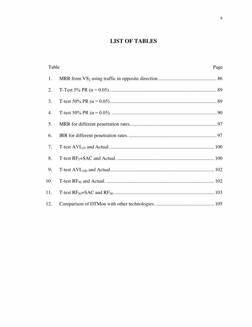
LIST OF TABLES
Table Page
1. MRR from VS2 using traffic in opposite direction ............................................... 86
2. T-Test 5% PR ( = 0.05) ....................................................................................... 89
3. T-test 50% PR ( = 0.05) ...................................................................................... 89
4. T-test 50% PR ( = 0.05). ..................................................................................... 90
5. MRR for different penetration rates. ..................................................................... 97
6. IRR for different penetration rates. ....................................................................... 97
7. T-test AVL25 and Actual. .................................................................................... 100
8. T-test RF5+SAC and Actual. .............................................................................. 100
9. T-test AVL100 and Actual.................................................................................... 102
10. T-test RF50 and Actual. ....................................................................................... 102
11. T-test RF50+SAC and RF50. ................................................................................ 103
12. Comparison of DTMon with other technologies. ............................................... 105

xi
LIST OF FIGURES
Figure Page
1. Generalized relationship among speed, density, and flow rate. ........................... 12
2. Functions of a TMC .............................................................................................. 17
3. Inductive loop detector system. ............................................................................ 26
4. Occlusion and its impact on video detection ........................................................ 29
5. Microwave radar operation. .................................................................................. 30
6. A sample header of a message or a report. ........................................................... 46
7. Illustration of virtual strips and segments. ............................................................ 50
8. Five dynamically defined virtual strips and two TOs. .......................................... 51
9. A sample volume-speed task. ............................................................................... 52
10. An illustration of TO and virtual strips in an intersection. ................................... 59
11. cdf of Ep in different PRs for medium flow rate. .................................................. 67
12. cdf of Ep in different PRs for medium-high flow rate. ......................................... 68
13. cdf of Ep in different PRs for high flow rate. ........................................................ 68
14. E[C] for different market penetration rate and traffic flow range. ....................... 69
15. The probability of success in forwarding through a 1000 meter segment. ........... 69
16. Relationship between distance d and probability of message reception freception. .. 73
17. An ability of a single TO in multi-branch roadways. ........................................... 74
18. Two TOs, desired virtual strip, and actual travel times. ....................................... 75
19. A six-lane bi-directional highway with two TOs and four VS. ............................ 82

xii
20. Expected inter-vehicle spacing for different market penetration rates. ................ 83
21. Freception based on the distance from the VS to TO1. ............................................. 84
22. MRR from VS2 with 50% PR. .............................................................................. 85
23. MRR from VS2 (1 km away) and VS5 (4 km away) with 50% PR. ..................... 86
24. Average message delay from VS2 with different delivery methods. .................... 87
25. Location of TOs and virtual strips ........................................................................ 94
26. MRR from VS2 using RF+SAC in different PRs. ................................................ 98
27. Estimated travel time by ILDs compared to actual. .............................................. 99
28. Average travel time ............................................................................................ 101
29. Travel time in 50% PR (aggregation every 5 minutes). ...................................... 103
30. SMS in 50% PR (aggregation every 5 minutes). ................................................ 104
31. SMS in 50% PR (aggregation every minute). ..................................................... 104
32. Message delay. .................................................................................................... 106
33. Flow rate at VS2 in 100% PR (aggregation every 5 minutes)............................. 108
34. Location of TOs and VS . ................................................................................... 110
35. TMS at virtual strips. Traffic stoppage occurs during 10-40 min. ...................... 111
36. Time, Space, and Speed. ..................................................................................... 112
37. Travel time for defined virtual segments. ........................................................... 112
38. Class diagram of the main components in our design. ....................................... 139
39. A small segment of a highway. ........................................................................... 146
40. The elapsed real time for 1 minute of dense traffic simulation. ......................... 149
41. A vehicle�’s displacement vs. velocity in a single simulation step ...................... 149
42. Comparison between average density results ..................................................... 154

xiii
43. Average difference in position (m) and average speed (m/s) .............................. 154
44. A sample plotted highway output for a 1000 m roadway. .................................. 156

1
CHAPTER 1
INTRODUCTION
State transportation departments in the US must collect and probe various types of data
for traffic monitoring purposes. Traffic management centers (TMCs) need high-quality
data regarding the status of roadways for monitoring and delivering up-to-date
information on traffic conditions to the traveling public. The most common of this traffic
data are traffic volume and flow rate, vehicle classification, traffic speed, traffic density,
travel time, and delay. Currently this data, such as speed and volume, is measured at
static points on the roadway using technologies that have significant maintenance
requirements. Systems that use this data to produce traffic reports are only as accurate as
the quality of the collected data. To obtain an accurate picture of traffic on any road
section at any time requires a real-time probe of vehicles traveling in that section. Current
technologies can only monitor vehicles at fixed points of interest and require
approximating some metrics, limiting the quality of the delivered data. Also fixed pointed
detectors may miss locations where congestion occur since they are often located away
from interchanges and other bottlenecks.
In the future, intelligent transportation systems - formed of combinational networks
(e.g. wireless, mobile, vehicular, and sensor networks) - will use roadside units that can
communicate with equipped vehicles (or mobile nodes) and with a TMC (a server). We
envision a near-term future where network communication devices are commonly
included in new vehicles. These devices will allow vehicles to form vehicular networks

2
allowing communication among themselves, other vehicles, and roadside units (RSUs) to
improve driver safety, provide enhanced monitoring to TMCs, and deliver real-time
traffic conditions to drivers. In this dissertation, we introduce a Dynamic Traffic
Monitoring mechanism (DTMon). We introduce RSUs called task organizers (TOs) that
can communicate with equipped vehicles and with a TMC. These TOs can be
programmed by the TMC to task vehicles with performing traffic measurements over
various sections of the roadway. Measurement points for TOs, or virtual strips, can be
changed dynamically, placed anywhere within near or far distance from the TOs, and
used to measure wide areas of the roadway network. This is a vast improvement over
current technology, where specific measurement points must be decided in advance and
hardware installed in those locations. Since vehicles are used to take traffic
measurements, TOs can report speed, travel times, and delays without needing
approximation even in low market penetration rates, and can report volume and density in
high market penetration rates. In addition to reporting traffic measurements to a TMC,
TOs can also be used to inform vehicles about the latest traffic conditions and other
useful information from the TMC.
In this chapter, we introduce the important traffic data and the vehicular ad-hoc
networks which can be used to probe and monitor this traffic data. Knowing the
importance of each type of traffic data, we propose DTMon, a dynamic traffic monitoring
mechanism using vehicular ad-hoc networks, TOs, and virtual strips, to augment and
improve the capability of the currently-used technologies. The thesis statement and
contributions are listed at the end of this chapter.

3
1.1. TRAFFIC DATA
The goals of monitoring traffic are directly tied to specific functional objectives of
departments of transportation (DOTs) and the related service providers, so the type of
data and its level of spatial or temporal aggregation vary depending on the ultimate use of
the data [1]. For example, some data are collected to support real-time traveler
information and traffic control, whereas other data are collected and used off-line to help
characterize typical travel patterns and project future traffic conditions. Examples of
some of the uses of traffic data include the following:
1. Predicting where roads should be built or expanded in the future
2. Designing bridges and pavements to withstand predicted traffic loads
3. Analyzing air quality in urban areas
4. Alerting drivers to congestion and accidents
5. Controlling traffic signals
Three basic variables, volume or flow rate, speed, and density, can be used to
describe traffic on any roadway. In addition to these variables, travel time and delay are
used to describe the traffic movement on any section of roadway [1, 2, 3].
1.1.1. Volume and Flow Rate
Volume and flow rate are two measures that quantify the amount of traffic passing a
point on a lane or roadway during a given time interval. These terms are defined as
follows:

4
Volume is the total number of vehicles that pass over a given point or section of a
lane or roadway during a given time interval; volumes can be expressed in terms
of annual, daily, hourly, or sub-hourly periods.
Flow rate is the equivalent hourly rate at which vehicles pass over a given point
or section of a lane or roadway during a given time interval of less than 1 hour,
usually 15, 10, or 5 minutes.
Volume and flow rate are variables that usually quantify demand, that is, the number
of vehicle occupants or drivers (usually expressed as the number of vehicles) who desire
to use a given facility during a specific time period. Congestion can influence demand,
and observed volumes sometimes reflect capacity constraints rather than true demand.
For example, in congested conditions demand is greater than volume because not
everyone that wants to use the road can access it.
The distinction between volume and flow rate is important. Volume is the number of
vehicles observed or predicted to pass a point during a time interval. Flow rate represents
the number of vehicles passing a point during a time interval less than 1 hour, but
expressed as an equivalent hourly rate. A flow rate is the number of vehicles observed in
a sub-hourly period, divided by the time (in hours) of the observation. For example, a
volume of 100 vehicles observed in a 15-minute period implies a flow rate of 100
veh/0.25 hour, or 400 veh/h. Also, flow rate can show the influence of sub-hourly
fluctuations in traffic which could cause variation in congestion.
Volume and flow rate can be illustrated by the volumes observed for four consecutive
15-min periods. For example, the four counts are 1000, 1200, 1100, and 1000. The total

5
volume for the hour is the sum of these counts, or 4300 vehicles. The flow rate, however,
varies for each 15-minute period. During the 15-minute period of maximum flow, the
flow rate is 1200 veh/0.25 h, or 4800 veh/h. Note that 4800 vehicles do not pass the
observation point during the study hour, but they do pass at that rate for 15 minutes.
1.1.2. Speed
Although traffic volumes provide a method for quantifying capacity values, speed is an
important measure of the quality of the traffic data provided to the TMC. Speed is a
measureable quantity of effectiveness, defining levels of service for many types of
facilities, such as rural two-lane highways, urban streets, freeway weaving segments, and
others. Speed can also be used to estimate travel time in some conditions.
Speed is defined as a rate of motion expressed as distance per unit of time, generally
as kilometers per hour (km/h). In characterizing the speed of a traffic stream, a
representative value must be used, because a broad distribution of individual speeds is
observable in the traffic stream. Usually the average travel speed is used as the speed
measure because it is easily computed from observation of individual vehicles within the
traffic stream and is the most statistically relevant measure in relationship to other
variables. Average travel speed is computed by dividing the length of the highway, street
section, or segment under consideration by the average travel time of the vehicles
traversing it. If travel times t1, t2, t3,..., tn (in hours) are measured for n vehicles traversing
a segment of length L, the average travel speed is computed using Equation 1.
(1)
where
6
S = average travel speed (km/h),
L = length of the roadway segment (km),
ti = travel time of the ith vehicle to traverse the segment (h),
n = number of travel times observed, and
ta = = average travel time over L (h).
The travel times in this computation include stopped delays due to fixed interruptions
or traffic congestion. They represent the total travel times to traverse the defined roadway
length. Several different speed parameters can be applied to a traffic stream. These
include the following:
Average running speed - A traffic stream measure based on the observation of
vehicle travel times traversing a section of highway of known length. It is the
length of the segment divided by the average running time of vehicles to traverse
the segment. Running time includes only the time that vehicles are in motion.
Average travel speed - A traffic stream measure based on travel time observed on
a known length of highway. It is the length of the segment divided by the average
travel time of vehicles traversing the segment, including all stopped delay times.
It is also a Space mean speed (SMS). It is called a space mean speed because the
average travel time weights the average to the time each vehicle spends in the
defined roadway segment or space.
Time mean speed (TMS) - The arithmetic average of speeds of vehicles observed
passing a point on a highway; also referred to as the average spot speed. The

7
individual speeds of vehicles passing a point are recorded and averaged
arithmetically.
Free-flow speed - The average speed of vehicles on a given facility, measured
under low-volume conditions, when drivers tend to drive at their desired speed
and are not constrained by control delay or congestion.
For most of the procedures using speed as a measure of effectiveness in this
dissertation, SMS and TMS are the defining parameters. For uninterrupted-flow facilities
like a segment of a highway or a street, the average travel speed is equal to the average
running speed.
SMS is always less than TMS, but the difference decreases as the absolute value of
speed increases. Based on the statistical analysis of observed data, this relationship is
useful because TMS often is easier to measure in the field than SMS [1, 2, 3]. To
calculate SMS accurately, average travel time must be calculated in an accurate way
which requires the observation of two constructing points of the segment rather than one.
It is possible to calculate both time mean and space mean speeds from a sample of
individual vehicle speeds. For example, suppose three vehicles are recorded with speeds
of 40, 60, and 80 km/h. The time to traverse 1 km is 1.5 min, 1.0 min, and 0.75 min,
respectively. The time mean speed is 60 km/h, calculated as (40 + 60 + 80)/3. The space
mean speed is 55.4 km/h, calculated as (60)[3 ÷ (1.5 + 1.0 + 0.75)].
1.1.3. Travel Time and Delay
Travel time is the amount of time that takes a vehicle to travel between two points on the
road. It is the piece of data most understandable for the driving public and, thus, is the

8
most desired data for traffic engineers. Historically, gathering travel times has been
challenging. Travel time is a variable used in calculation of average running speed and
average travel speed and also space mean speed.
Delay, or expected delay, is also a piece of data useful for the driving public. This is
the time difference between the observed travel time of the road segment and the travel
time usually measured directly by knowing the length of the segment and the desired
speed on that segment. For example, the travel time for a 5 km segment of a roadway
with a speed limit (desired speed) of 80 km/h is 0.0625 h (1 km ÷ 80 km/h). If the
observed average travel time of the vehicles that have passed the same segment is 0.09 h,
then the average delay can be estimated as 0.0275 h (1.65 min). This delay can be
assumed as the average delay that the drivers have encountered during their journey
through the segment or can be used as an estimate for the expected delay, the delay that
drivers may expect to encounter upon entering the same segment.
1.1.4. Vehicle Classification
Vehicle classification data records traffic volume with respect to the type of vehicle that
passes a point on the road. The Federal Highway Administration (FHWA) has defined a
set of 13 vehicle classes that are commonly used by most states [1, 3]. In addition to
vehicle classification, TMC needs the percentage of vehicles in different classes which
pass a point on the road. The classification scheme is separated into categories depending
on whether the vehicle carries passengers or commodities. Non-passenger vehicles are
further subdivided by number of axles and number of units, including both power and

9
trailer units. The most common vehicle types are motorcycles, buses, passenger cars
(including all sedans, coupes, and station wagons), and trucks.
1.1.5. Density
Density is the number of vehicles occupying a given length of a lane or roadway at a
particular instant. For the computations in this dissertation, density is usually averaged
over time and is usually expressed as vehicles per kilometer (veh/km).
Direct measurement of density in the field is difficult, requiring a vantage point for
photographing, videotaping, observing significant lengths of highway, or surrogating
based on other metrics. Density can be computed, however, from the average travel speed
and flow rate, which are measured more easily. Equation 2 is used for under-saturated
traffic conditions.
(2) where
v = flow rate (veh/h),
S = average travel speed (km/h), and
D = density (veh/km).
A highway segment with a rate of flow of 1000 veh/h and an average travel speed of
50 km/h would have a density of
Density is a critical parameter because it characterizes the quality of traffic
operations. It describes the proximity of vehicles to one another and reflects the freedom
to maneuver within the traffic stream.

10
Roadway occupancy is frequently used as a surrogate for density in control systems
because it is easier to measure. Occupancy in space is the proportion of roadway length
covered by vehicles, and occupancy in time identifies the proportion of time a roadway
cross section is occupied by vehicles.
1.1.6. Headway and Spacing
Spacing, or space headway, is the distance between successive vehicles in a traffic
stream, measured from the same point on each vehicle (e.g., front bumper, rear axle, etc.).
Headway, or time headway, is the time between successive vehicles as they pass a point
on a lane or roadway, also measured from the same point on each vehicle.
These characteristics are microscopic, since they relate to individual pairs of vehicles
within the traffic stream. Within any traffic stream, both the spacing and the headway of
individual vehicles are distributed over a range of values, generally related to the speed of
the traffic stream and prevailing conditions. In the aggregate, these microscopic
parameters relate to the macroscopic flow parameters of density and flow rate.
Spacing is a distance, measured in meters. It can be determined directly by measuring
the distance between common points on successive vehicles at a particular instant. This
generally requires complex techniques, so that spacing is usually derived from other
direct measurements. Headway, in contrast, can be easily measured with time
observations as vehicles pass a point on the roadway. Since headway and spacing are
related, knowing the headway allows the spacing to be determined as shown in Equation
3.

11
The relationship between average spacing and average headway in a traffic stream
depends on speed, as indicated in Equation 3.
(3)
This relationship also holds for individual headway and spacing between pairs of
vehicles. The speed is that of the second vehicle in a pair of vehicles.
The average vehicle spacing in a traffic stream is directly related to the density of the
traffic stream, as determined by Equation 4.
(4)
Flow rate is related to the average headway of the traffic stream as shown in Equation
5.
(5)
1.1.7. Relationship Among Basic Parameters
Equation 2 cites the basic relationship among the parameters density, speed, and flow
rate, describing an uninterrupted traffic stream. Although the equation v = S * D
algebraically allows for a given flow rate to occur in an infinite number of combinations
of speed and density, there are additional relationships restricting the variety of flow
conditions at a location.
Figure 1 shows a generalized representation of these relationships, which are the
basis for the capacity analysis of uninterrupted-flow facilities like in highways and streets
where relationship between speed and density is assumed to be linear. Speed is space
mean speed.

12
Figure 1. Generalized relationship among speed, density, and flow rate (based on
[2]).
The form of these functions depends on the prevailing traffic and roadway conditions
on the segment under study and on its length in determining density. Although the
diagrams in Figure 1 show continuous curves, it is unlikely that the full range of the
functions would appear at any particular location. Survey data usually show
discontinuities, with part of these curves not present.
The curves of Figure 1 illustrate several significant points. First, a zero flow rate
occurs under two different conditions. One is when there are no vehicles on the roadway,
thus both density and flow rate are zero. Speed is theoretical for this condition and would

13
be selected by the first driver (presumably at a high value). This speed (the free flow
speed) is represented by Sf in Figure 1.
The second case is when density becomes so high that all vehicles must stop�—the
speed is zero, and the flow rate is zero, because there is no movement and vehicles cannot
pass a point on the roadway. The density at which all movement stops is called jam
density, denoted by Dj in Figure 1.
Between these two extreme points, the dynamics of traffic flow produce a
maximizing effect. As flow increases from zero, density also increases, since more
vehicles are on the roadway. When this happens, speed declines because of the
interaction of vehicles. This decline is negligible at low and medium densities and flow
rates. As density increases, these generalized curves suggest that speed decreases
significantly before capacity is achieved. Capacity is reached when the product of density
and speed results in the maximum flow rate. This condition is shown as optimum speed So
(often called critical speed), optimum density Do (sometimes referred to as critical
density), and maximum flow vm.
The slope of any ray line drawn from the origin of the speed-flow curve represents
the inverse of density, based on Equation 2. Similarly, a ray line in the flow-density graph
represents speed. As examples, Figure 1 shows the average free-flow speed and speed at
capacity, as well as optimum and jam densities. The three diagrams are redundant, since
if any one relationship is known, the other two are uniquely defined.
As shown in Figure 1, any flow rate other than capacity can occur under two
different conditions, one with a high speed and low density and the other with high

14
density and low speed. The high-density, low-speed side of the curves represents
oversaturated flow. Sudden changes can occur in the state of traffic (e.g., in speed,
density, and flow rate). We emphasize that these are theoretical relationships based on a
linear speed-density relationship. Empirical data differs from these somewhat.
1.2. Vehicular Ad-hoc Networks
A Vehicular Ad-Hoc Network, or VANET, is a technology that uses vehicles (usually
moving vehicles) as nodes in a network to create a mobile network. Therefore, VANET is
a form of mobile ad-hoc network [4, 5]. Vehicles in VANETs are able to communicate
with nearby vehicles and between vehicles and nearby fixed equipments. The main goal
of VANETs is to provide safety and comfort for passengers. There are several
applications for VANETs such as incident management, collision warning, vehicle
tracking, improved driving, resource awareness, etc. [5]. There may also be multimedia
and Internet connectivity facilities for drivers (passengers), all provided within the
wireless coverage of each vehicle. Automatic payment for parking lots and toll collection
are other examples of possibilities using VANETs.
An on-board unit (OBU) consists of a wireless transceiver in a vehicle that provides
the communication with nearby road-side units (RSU) using Dedicated Short Range
Communication (DSRC). DSRC [6] provides short-to-medium range wireless
communication channels (5.9 GHz up to range of 300 meters) specifically designed for
automotive use. There are a corresponding set of protocols and standards (IEEE 1609 [7],
IEEE 802.11p [8]) associated with DSRC. Vehicles are also able to store useful data

15
during their trip for later delivery. The information gathered by OBUs and RSUs can be
mined to derive traffic data and its derivatives.
The main advantages of using VANETs in monitoring traffic compared with other
technologies are as follows:
1. VANETs can be used to collect and monitor real time traffic speeds and travel
times.
2. VANETs can be used to collect and monitor real time information on congestion.
3. VANETs have the potential to be used to dynamically change traffic signal
timings.
4. There are two-way communications between vehicles and roadside units in
VANETs.
5. VANETs have the potential to provide up-to-date traveler information in addition
to safety messages.
6. RSUs are nonintrusive.
The initial disadvantages are as follows:
1. VANET is still in its infancy, and the technology and requirements have not been
thoroughly tested and evaluated.
2. Its reliability and accuracy must be ensured.
3. Like other probe vehicle-based methods, VANET suffers when the market
penetration rate and sample size are low.
4. Its cost is still unknown. (OBU, RSU, operating, maintenance, etc.)

16
In Chapter 3, we will explain the use of VANETs in our proposed framework
(DTMon) and its components in more detail.
1.3. Traffic Management Centers
The TMC serves as the focal point for the management of the roadway transportation
system in an area [3]. It integrates data from a variety of different sensor sources and
provides a means for operators to manage traffic and inform the public from a centralized
point. Many TMCs are also co-located with emergency responders to help facilitate
coordination when a crash or other emergency arises. The workstations offer
functionality to perform tasks like changing messages on dynamic message signs
(DMSs), viewing police dispatch reports, and controlling closed-circuit cameras.
Sensors and other detection devices can usually communicate and transfer data with
the TMCs through wired, wireless, or by portable data storage [3, 9, 10]. Wired
mechanism involves regular cable, fiber optic cables (higher bandwidth), or telephone
lines. Wireless transfer of data can be done through cell phones or radio frequencies
specified for this purpose. Portable data storage devices are usually located nearby
sensors or attached to them. They store data which will be transferred to TMCs for
archiving or off-line data processing.
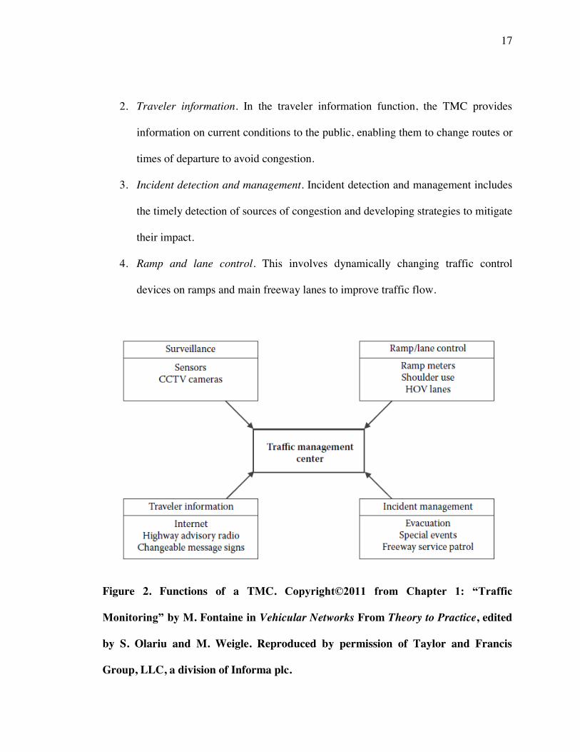
The major functions of the TMC are the following (see Figure 2):
1. Surveillance. The surveillance function involves the collection of data on traffic
flow conditions on the roadways being monitored.
17
2. Traveler information. In the traveler information function, the TMC provides
information on current conditions to the public, enabling them to change routes or
times of departure to avoid congestion.
3. Incident detection and management. Incident detection and management includes
the timely detection of sources of congestion and developing strategies to mitigate
their impact.
4. Ramp and lane control. This involves dynamically changing traffic control
devices on ramps and main freeway lanes to improve traffic flow.
Figure 2. Functions of a TMC. Copyright©2011 from Chapter 1: �“Traffic
Monitoring�” by M. Fontaine in Vehicular Networks From Theory to Practice, edited
by S. Olariu and M. Weigle. Reproduced by permission of Taylor and Francis
Group, LLC, a division of Informa plc.

18
1.4. THESIS STATEMENT AND CONTRIBUTIONS
There are several sensors/detectors and technologies currently used to monitor traffic data
(see Chapter 2 Sections 2.1 and 2.2). These traffic data are usually monitored by
technologies such as inductive loop detectors (ILDs), video detection systems, acoustic
tracking systems, and microwave radar sensors (MRS). In addition, wireless technologies
are used in systems such as automatic vehicle identification (AVI), automatic vehicle
location (AVL), and wireless location technology (WLT).
Among these, ILDs are the most prevalent, generally have the highest accuracy, and
can monitor all of the fundamental traffic data except travel times. However, they are
prone to failure. Maintenance, installation, and replacement can be problematic, and
because of this, large portions of an ILD network may not be returning quality data at any
given time. Video detection systems have issues in inclement weather (e.g., fog, rain,
snow) and especially with occlusion. Occlusion is also a major problem for acoustic
tracking and microwave radar systems. The ability of AVI-based systems to provide
useful data is directly linked to the number of probes on the road. Therefore, these
systems require the installation of significant roadside infrastructure to detect equipped
vehicles. AVL systems are susceptible to the same sample size limitations as AVI
systems. Also, trucking companies have been reluctant to share their AVL data with
others due to concerns about losing competitive advantages in the marketplace, so data
sources are not widely available. Note that AVL devices can also be installed in
municipal buses or taxis. WLT systems are based on the presence of cellular phones in

19
vehicles for monitoring traffic. But, these systems do not have the same location
precision as GPS and cannot distinguish between different phones in the same vehicle.
Thesis Statement: Vehicular networks and in particular DTMon, a dynamic traffic
monitoring system consisting of task organizers (programmable road side units) and
virtual strips (dynamic points of interest), can be used to efficiently provide to TMCs
high-quality, fine-grained traffic measurements covering a large area of the roadway.
This thesis is a framework for designing various systems that could be deployed in
different configurations based on highway topology and traffic conditions. We will
analyze the capabilities of DTMon and TOs to monitor high-quality traffic data in various
traffic conditions (free-flow and congested states). For some types of data, the percentage
of equipped vehicles, or the penetration rate, affects the quality of data gathered. We will
investigate methods for mitigating the effects of low penetration rate as well as low
traffic density on data quality. This may include deploying multiple TOs in a region or
using oncoming traffic to help bridge gaps in connectivity.
Our framework, and in particular DTMon, can have a large impact on traffic
monitoring. Traffic engineers can take advantage of the programmability of TOs, giving
them the ability to measure traffic at any point within up to reasonably far distances from
TO. Since the location of virtual strips can be changed at any time, measurement points
can be adjusted as traffic conditions change. An important example of this is end-of-
queue management. Traffic engineers are very interested in monitoring the endpoints of
congestion and would like to deliver timely information to drivers approaching these
points to improve safety. Another important example of the usefulness of dynamic

20
measurement is an evacuation scenario. As drivers evacuate, they may take roadways that
are not normally monitored. A TO could be placed temporarily in those locations as
conditions mandate to measure traffic and provide important information to drivers. Most
real-time traffic maps measure traffic at midpoint of roads between interchanges and the
use of this framework would allow for virtual strips to be placed at various locations in
between interchanges, providing fine-grained measurements to TMCs. Maybe most
importantly, a single TO could be used to monitor traffic up to reasonably far distances,
resulting in lower monitoring costs with less delay than is currently possible in providing
real-time information from/to drivers.
Contributions:
1. A method for using probe vehicles to perform spatial sampling of traffic
conditions �– Probe vehicles can provide real-time measurements of speed and
travel time. Using spatial sampling allows for these measurements to be made at
specific locations of interest on the roadway. This avoids the need for
interpolation and estimation that is required when temporal sampling of probe
vehicles is performed.
2. An analysis of the factors that can impact the quality of monitored traffic data
when using vehicular networks �– These factors are market penetration rate, traffic
conditions, communication range, distance between communicating entities,
methods of message delivery, message reception rate, and message delay. We
have performed an analysis of these factors and how each contributes to the

21
quality of traffic data that can be reported. We note that both traffic conditions
and market penetration rate affect the distance between communicating entities.
3. An evaluation of the impact of different methods of message delivery on the
quality of traffic data that can be gathered by vehicular networks �– We compared
four different message delivery methods (regular forwarding, dynamic
transmission range, store-and-carry, and a hybrid approach) by measuring
message reception rate and message delay in different traffic conditions and
different market penetration rates. We found that a hybrid approach (regular
forwarding coupled with store-and-carry and using vehicles traveling in the
opposite direction) can significantly improve the performance of DTMon in
poorly connected traffic conditions. We also showed that when the market
penetration rate is high, the message delay can be reduced significantly.
4. An evaluation of the effectiveness of DTMon as compared with current
technologies such as inductive loop detectors (ILD) and automatic vehicle
location (AVL) �– We show that DTMon can be used to report travel times that are
not statistically different from the actual travel times. In comparison, we show
that technologies such as ILD cannot measure travel times with this level of
accuracy.
5. A demonstration of the usefulness of DTMon�’s monitoring approach for
monitoring congested traffic conditions �– We have shown the ability of DTMon
to allow a TMC to dynamically place additional monitoring points (virtual strips)
in locations where congestion is building up. This allows the TMC to detect

22
transitions in traffic flow using speeds and travel times, without having to rely on
flow rate information. We have shown that DTMon can be used to detect and
track the end-of-the-queue in traffic with congestion.
6. Highway mobility modules for the ns-3 network simulator �– We have contributed
the first highway mobility modules designed to produce realistic vehicle mobility
and communications in ns-3. The mobility model has been validated against the
well-known vehicular mobility models, and the networking components use ns-3,
which has been validated against wireless models. These modules have been
released to the ns-3 community and are now being used by other researchers
around the world.
1.5. OUTLINE
The dissertation is organized as follows:
Chapter 2 presents the background and related work for the proposed DTMon and
implemented integrated VANET simulator. We also present the background and
related work regarding traffic monitoring using technologies such as
sensors/detectors and probe vehicle-based systems.
Chapter 3 introduces and explains the components of DTMon for dynamic traffic
monitoring using VANETs. We describe the main components of the proposed
framework such as proposed task organizers, proposed virtual strips and segment,
equipped vehicles and methods/techniques to monitor traffic data. We analyze the
effect of the market penetration rate and the traffic density on DTMon�’s
performance. We explain various scenarios and strategies for deploying TOs. We

23
also describe the advantages of TOs and dynamically defined virtual strips in
augmenting the current in-use systems for monitoring traffic.
Chapter 4 evaluates the proposed methods in free-flow traffic and addresses the
effect of traffic flow, speed, density, and market system penetration rate on
monitoring high quality traffic data. We show the performance of various
methods of message delivery on information and message reception rate and
delay in monitoring high quality traffic data. In addition to free flow traffic, we
evaluate the proposed methods in traffic with congestion and addresses the effect
of traffic flow, speed, density, and market system penetration rate on monitoring
high quality traffic data. We show the performance of various methods of
message delivery and compare the results with sensors/detectors and probe
vehicle-based systems. We also show advantage of using our dynamic monitoring
in detecting congestion.
We conclude and summarize our research and achievements in Chapter 5. We
discuss future research directions in Chapter 5 as well.
Appendix A presents the first implementation of a well-known vehicle mobility
model in ns-3, the next generation of the popular ns-2 networking simulator. We
show the need and motivation for a quality integrated VANET simulator which
was used to evaluate our proposed dynamic traffic monitoring system.

24
CHAPTER 2
BACKGROUND AND RELATED WORK
In the United States and numerous other parts of the world, road traffic is a critical part of
a region�’s economic activity. Numerous measures are taken to address problems arising
from traffic flow, its transition, and congestion. An essential step in this direction is the
creation of a traffic monitoring system with capabilities to estimate traffic data with
significant accuracy and reliability. Historically, dedicated infrastructure has been used
for monitoring traffic data, however, the corresponding sensors have limited coverage,
high installation and maintenance costs, and their fixed position does not enable
optimized and adaptive sampling as traffic conditions change. Therefore, there is a need
for a mechanism which can augment these monitoring systems or even replace them.
In this chapter, we present traffic monitoring methods and technologies. We explain
the advantages and disadvantages of these technologies.
2.1. TRAFFIC MONITORING METHODS AND TECHNOLOGIES
There are several sensors and detectors, methods, and technologies that can be used to
collect, probe, and monitor traffic data [3, 9, 10]. The sensor technologies can be broadly
classified into two categories: intrusive and nonintrusive sensors.
Intrusive detectors require intrusion into the pavement to perform installation or
maintenance activities.
Nonintrusive detectors are mounted either above or beside the roadway.

25
An example of an intrusive detector would be an inductive loop detector (ILD)
installed in the pavement surface. Intrusive detectors in comparison to nonintrusive
detectors have several problems:
1. Travel lanes may have to be closed in order to perform maintenance on the
sensor.
2. Timely maintenance, particularly in a congested urban area, is a significant barrier
where it may be difficult to close lanes during the day due to the impact on traffic.
3. They need to be replaced every time a road is repaved.
In addition to sensors, a number of new monitoring methods that rely on the use of
probe vehicle data have been deployed as a way to gather traffic data mostly relating to
travel time and speed. Probe vehicle-based systems track the movements of a subset of
the vehicle population in order to estimate the travel characteristics of all vehicles on the
road. Probe vehicle systems can generate estimates of speed and travel time on a section
of road, but they generally do not produce estimates of the volume or density of traffic.
By using this approach, estimates of SMS (rather than TMS) are generated for the road.
Thus, the speed estimates more fully characterize what drivers actually experience [2, 3,
9]. One method to probe traffic data is the use of wireless technology such as cell phones.
In this section, we introduce these commonly used sensors, methods, and
technologies in addition to their connectivity to TMC.
2.1.1. Inductive Loop Detectors
Inductive loops are intrusive detectors, consisting of a coiled wire that is cut into the
pavement. The ILD senses the presence of metal objects that pass over the coiled wire.

26
When a vehicle passes over or stops on top of an ILD, it reduces the loop inductance of
the wire. Currents are induced in the vehicle, reducing loop inductance. The reduction in
loop inductance is then translated by a controller into a detection of the presence of a
vehicle (see Figure 3). Lengths of vehicles can be estimated, but the number of axles is
not explicitly counted.
Figure 3. Inductive loop detector system.
ILDs can be installed as either a single or double loop configuration. Single loop
detectors comprise just one loop of coiled wire installed in the pavement and are
generally used to provide traffic volume and density information. With double loops, two
loops are installed in a lane of road one after another, with a short space between the two
ILDs. Double loops are necessary to generate speed estimates. As the two ILDs are
placed a known distance apart, the speed of a vehicle can be estimated by examining the
time that elapses between the activations of the two loops.
There are also several advantages to using ILDs:
1. The technology is mature, and there is a large experience base with the sensors.
2. All of the fundamental traffic data including volume, occupancy, TMS, and
vehicle classification can be provided by ILDs.

27
3. ILDs are robust to inclement weather such as fog, rain, and snow.
4. ILDs generally have the highest accuracy of commonly used sensors, with
accuracy reported to be between �–1 and +2% across a variety of studies [11, 12].
5. ILDs can produce high quality data (i.e., flow rate and volume).
Disadvantages of ILDs are as follows:
1. ILDs require regular tuning to ensure that speeds and vehicle classification data
are of high quality.
2. They are intrusive sensors, therefore maintenance, installation, and replacement of
ILDs can be problematic, particularly in congested urban areas.
3. Multiple loops are usually required to monitor a location.
4. Detection accuracy may decrease when design requires detection of a large
variety of vehicle classes.
5. They are prone to failure, and large portions of an ILD network may not be
returning quality data at any given time because of ILD failure rates and
maintenance difficulties.
For example, in 2005 the Virginia Department of Transportation Traffic Management
Center in Hampton Roads estimated that about 40% of their ILDs were not returning
quality data [13]. The difficulties in maintaining ILDs have been a significant reason why
alternative detection technologies have been pursued.
2.1.2. Video Detection System
Video detection systems utilize cameras and image processing software to collect data on
traffic flow. A camera is pointed at a roadway, and image processing software analyzes

28
changes in pixels between successive frames. The processing software identifies when a
vehicle has entered the frame, and then translates the movement of the vehicle on the
video into traffic flow parameters [9, 10].
Video detection offers several advantages over ILDs:
1. Video detection systems are nonintrusive detectors which can collect all of the
same traffic flow parameters as inductive loops.
2. A single controller and camera combination can be used to detect multiple lanes
on an approach.
3. Wide-area detection can be provided when information gathered from multiple
camera locations are linked together.
4. Video detection system is sometimes more cost effective solution for traffic
signal detection over the lifecycle of the equipment.
The problems with video detection systems are as follows:
1. Some periodic maintenance, such as cleaning camera lenses, requires shutting
down lanes.
2. Video detection systems have issues in inclement weather (i.e., fog, rain, snow)
which can create problems with the video processing software because they
reduce the contrast in the image between vehicles and the background.
3. The field of view of the camera can be affected by high winds.
4. Reliable nighttime signal actuation requires street lighting.
5. Occlusion is a major potential problem with video detection systems (see Figure
4) [3, 4].

29
Occlusion occurs when a vehicle obscures another vehicle within the camera�’s field
of view. Occlusion can cause undercounting of traffic volumes or poor speed estimation.
Figure 4. Occlusion and its impact on video detection. Copyright©2011 from
Chapter 1: �“Traffic Monitoring�” by M. Fontaine in Vehicular Networks From
Theory to Practice, edited by S. Olariu and M. Weigle. Reproduced by permission of
Taylor and Francis Group, LLC, a division of Informa plc.
2.1.3. Microwave Radar Sensors
Microwave radar sensors (MRS) are devices for transmitting high frequency
electromagnetic signals and receiving echoes from objects of interest within their volume
of coverage.
MRS have flexibility in where they can be placed. The sensors are typically mounted
on existing structures that pass over the highway (such as sign structures or bridges) or on

30
posts adjacent to the roadway, therefore MRS are another alternative option to ILDs, and
have the following advantages:
1. MRS are nonintrusive.
2. They can directly measure speed.
3. They can provide volume, occupancy, TMS, and vehicle classification data.
4. They can be mounted to collect data for a single lane or to collect data across
multiple lanes.
5. They are typically insensitive to inclement weather at relatively short ranges.
MRS have disadvantages:
1. The accuracy of MRS is not as good as well-functioning ILDs.
2. MRS suffer from many of the same occlusion problems as video detection.
3. They cannot detect stopped vehicles and vehicles with low speed.
Figure 5. Microwave radar operation.

31
The most common application of microwave sensors is to supplement data collected
from ILDs on major freeway facilities. Infrared, ultrasonic, and acoustic radars are fairly
similar technologies that are used for detection of vehicles, but these technologies do not
perform as accurately as MRS in various conditions and are not used as widely as ILDs,
cameras, and MRS for monitoring traffic data.
2.1.4. Automatic Vehicle Identification
Automatic Vehicle Identification (AVI) systems are probe vehicle-based systems that
usually rely on tags which reflect encoded radio signals transmitted from roadside
antennas or readers. The reflected signals are modified by the tag identification code so
that the tag�’s information can be read by the system. This type of system has also been
adapted to collect traffic monitoring data. In a monitoring application, roadside antennas
are installed along major highways where the DOT wants to collect information on travel
times or speeds. The unique tag identification numbers are logged each time a vehicle
passes by an antenna.
The travel time of the vehicle can then be explicitly calculated by examining when a
vehicle passes known antenna locations on the highway. This provides true point-to-point
travel times for all vehicles with tags. An example for this method is the system of toll
transponders and vehicles�’ smart tags.
There are several issues related to the deployment of AVI-based monitoring systems:
1. The ability of AVI-based systems to provide useful data is directly linked to the
number of potential probes on the road.

32
2. A sufficient number of probe vehicles must travel a route for the travel time and
speed estimate to have statistical validity.
3. These systems require the installation of significant roadside infrastructure in the
form of AVI tag readers and communications in order to gather data.
4. These systems have significant cost.
Capital costs for a single AVI site on a six-lane highway range from $18000 to
$38000, with annual operating costs of $4000 to $6000 per site [14, 15]. If sites are to be
spaced every 2 to 3 kilometers, this can be a significant cost. The advantage these
systems have is that they can produce quality speed and travel time estimates.
2.1.5. Automatic Vehicle Location
Automatic Vehicle Location (AVL) refers to a suite of probe vehicle-based technologies
that track the location of vehicles traveling through the roadway network. The more
commonly-used method in AVL relies on global positioning system (GPS) data. GPS
data is collected continuously by the vehicle and then periodically transmitted back to a
central control facility over a radio backbone, cellular service, or satellite
communications network. The location data generated by AVL systems could be mined
to generate traffic data. Examples for such a system are transit companies which track
location of buses on their routes [16] and combined traffic information providers such as
INRIX [17] which fuse their data from several sources including AVL systems (usually
from equipped trucks, buses, taxis, etc.).
The advantages of using this system are as follows:
1. Few pieces of fixed infrastructure are required.

33
2. Vehicles could be monitored anywhere on the network.
3. AVL technologies can provide estimates of speed and travel times on roads where
no point sensors (i.e., ILDs, MRS, cameras) are available.
This system has several limitations:
1. AVL has problem with the sample size limitations where only a small subset of
the vehicle population is outfitted with AVL equipment.
2. The estimated travel time and speed includes the stop and load delay time of
equipped vehicles during their trip (see Section 1.1.2).
3. The data source is also not widely available since participant companies may not
share their data with others due to concerns about losing competitive advantages
in the marketplace.
4. Usually the routes (i.e., AVL drivers�’ path) are predictable and the generated data
using AVL are not enough for monitoring the entire region.
2.1.6. Wireless Location Technology
Wireless Location Technology (WLT) involves using wireless devices to track the
vehicle (generally the mobile passenger) movements or to transfer information from the
vehicles for monitoring purposes. WLT systems are mostly based on the presence of
cellular phones in vehicles for monitoring traffic. An example for such system is
anonymous tracking of cellular phones [3, 18, 19]. WLT based traffic monitoring has the
potential to expand both the number of vehicles being monitored and the size of the
roadway network where data could be obtained.
The advantages of WLT using cellular phones are as follows:
34
1. A majority of car owners own cell phones.
2. Any road with cellular service can theoretically be monitored without installing
any infrastructure on the road.
3. Aggregated data are not particular to the fixed points on the road and can provide
information about several sampled locations on the road.
The major barriers to widespread use of WLT-based monitoring are as follows:
1. The spatial accuracy of the location estimates used by WLT systems is not as
precise as GPS data. (e.g., existing systems cannot distinguish between different
phones in the same vehicle or even determine differences in travel speeds between
adjacent lanes of traffic.)
2. Producing precise estimates of speed and travel time is highly affected by the
precision of location estimates.
3. WLT has issues with the continuous consumption of bandwidth on the wireless
link which can also cause congestion in the wireless network, information drops,
or unwanted handoffs.
4. Questions about who owns the data and what rights a DOT has to distribute the
data still remain since the data is generated by a third party vendor that sells the
data as a service to a DOT.
5. Privacy of users in these systems is questionable.
2.2. USE OF CELLULAR NETWORKS AND SMARTPHONES
An alternative to using dedicated sensing infrastructure is to leverage an existing
communication systems such as the cellular phone network. The mobile Internet and

35
Web 2.0 are the underlying technologies and paradigms that have enabled the
development of traffic estimation systems based on GPS-enabled phones as well as
numerous other cellular device-based traffic monitoring systems. WLT systems are based
on the presence of cellular phones in vehicles for monitoring traffic. But, these systems
do not have the same location precision as GPS and cannot distinguish between different
phones in the same vehicle. In addition, since these systems report data based on at a
particular time, it is difficult to collect data at a certain location. In this dissertation, when
we mention WLT systems we mean systems that rely on cellular network based
positioning and handsets that do not use GPS. Although, handsets may be equipped with
GPS device too.
There are several projects developing the use of wireless technology for traffic
monitoring, such as PATH�’s Group-Enabled Mobility and Safety (GEMS) project [20].
GEMS is based on AVL and WLT technologies with use of Internet queries for
delivering data to handheld devices. In the Mobile Millennium project [19], cell phones
are the main part of the architecture. The project�’s concept of virtual lines is similar to
our proposed virtual strips, which we propose and describe in Chapter 3. Using the
mobile Internet, user-generated content (in this case, traffic data measured by the smart-
phone) is sent to a central system, which provides information back to the cell phone
owner for personal use. This Web 2.0 user-generated content-based location based
service is commonly referred to as �“participatory sensing�”, which refers to the ad-hoc
process of voluntarily providing sensing data to a system. GPS-equipped vehicles
transmit data upon traversing virtual geographical sensors, thus offering a promising

36
alternative to estimating traffic statistics using fixed point-sensors. This sensing
technique leverages market-driven telecommunication infrastructure, thus limiting cost
for society and users. Moreover, these virtual sensors, by definition, are not embedded in
the physical infrastructure, and their location can be optimized dynamically (adaptively)
as traffic conditions change. The location of the sensors can be dictated by the central
system to optimize the value of each traffic sensor measurement sent to the system.
The Nericell project [21] is another example of using cellular networks and smart-
phone for monitoring of road and traffic conditions. Nericell system uses mobile smart-
phones equipped with an array of sensors (GPS, accelerometer, microphone) and
communication radios. This project mainly focuses on the sensing components which are
installed or setup on smart-phones, and specifically focuses on how these sensors and
radios are used to detect bumps and potholes, braking, and honking, and to localize the
phone in an energy-efficient manner. While GPS provides higher accurate location
estimates compared to cellular technologies, it has several limitations such as some
phones do not have GPS at all and the GPS sensor does not work in �“urban canyons�” (tall
buildings and tunnels) or when the phone is inside a pocket. Also the GPS on many
phones is power-hungry and drains the battery quickly. The VTrack system [22]
addresses these key challenges (e.g., energy consumption and sensor unreliability). In
VTrack, energy consumption can be reduced using inaccurate position sensors (WiFi
rather than GPS). VTrack uses a hidden Markov model (HMM)-based map matching
scheme, with a way to interpolate sparse data to identify the most probable road segments

37
driven by the user and to attribute travel times to those segments, to obtain accurate travel
time estimates from these inaccurate positions.
Besides the value of the data for traffic estimation, ensuring location privacy of the
users is an important consideration for the deployment of mobile traffic sensing methods.
A GPS-enabled smartphone is capable of recording and transmitting its GPS location
every few seconds. While this level of detail can be useful for traffic estimation [23], it
can be privacy invasive without the proper safeguards, since the device is ultimately
carried by a single user.
We describe the advantages of using virtual strips and spatial sampling in Chapters 3.
The same idea can be used via WLT systems. For example, Virtual Trip Lines (VTLs),
similar to our contributed virtual strips, provide a mobile sensing framework that
preserves the privacy of users [24]. VTLs are geographical markers embedded in the
map, that trigger probabilistic measurement updates. Each VTL consists of two GPS
coordinates which make a virtual line drawn across a roadway of interest. Instead of
time-based periodic sampling, VTLs trigger disclosure of speed and location updates by
spatial sampling, creating updates at predefined geographic locations on roadways of
interest. Additionally, the travel time between pairs of VTLs can be extracted and this
type of travel time data will be considered the primary data source used in this approach.
This sensing paradigm of virtual trip lines has emerged as a viable solution for real-time
traffic monitoring based on large-scale traveler participation. However, standard VTL
deployment is static and does not take advantage of the mobility of probes compared to
our proposed DTMon where virtual strips are defined dynamically.

38
2.3. USE OF VEHICULAR NETWORKS AND SENSOR NETWORKS
VANETs are networks in which each node is a vehicle. Such systems aim to provide
communications between individual vehicles and between vehicles and nearby fixed
equipment, or roadside units. The goal of VANETs, and more broadly vehicular
networks, is to improve traffic safety by providing timely information to drivers and
concerned authorities. The development of VANETs has received much attention from
the automotive industry and government agencies, including the US Department of
Transportation (DOT) which has launched the Connected Vehicle initiative [25, 26].
There have been a few attempts at using VANETs to monitor traffic. TrafficView
[27] is a scalable traffic monitoring system for inter-vehicle communication considering
road conditions, but it does not consider low penetration rates or low traffic density.
CarTel [28] is distributed mobile sensor computing system that uses cell phones and cars
as nodes in a dynamic sensor network. CarTel provides software to collect, process, and
visualize data from sensors located on mobile devices to a central portal. Kitani et al. [29]
have proposed traffic information sharing using public buses traveling regular routes.
This VANET-based technique is only useful in urban areas with good public
transportation systems and only monitors those areas traveled by the transit system.
As we show in Chapter 3, one of our main contributions is the first introduction of
location-aware sensing strategies via VANETs (using DTMon and virtual strips) that are
adaptive to the traffic conditions, thereby enabling the sensing infrastructure (i.e., TOs) to
take full advantage of the mobility of probes. TOs programmed by TMCs can also define
the points of interest dynamically in addition to that in DTMon, TOs are also able to

39
redefine, modify, add, or remove these virtual strips dynamically based on the monitored
traffic condition and real-time monitoring needs. We show the performance of DTMon in
various traffic conditions in Chapter 3. The main difference between the WLT systems
and our proposed DTMon is the base technology used in our framework. The technology
used in DTMon relies on vehicular ad-hoc networks than cellular networks. There has
been some work done in Connected Vehicle Research for traffic monitoring under low
penetration rates [25, 26]. But, there has been no work done on monitoring traffic
dynamically using VANETs for various traffic conditions and market penetration rates.
Therefore we believe our research, the proposed framework, and experiments perfomred
using DTMon will be a pioneer in real-time traffic monitoring with benefits of
dynamically defined spatial criteria. We also believe that our work on the
programmability of TOs can easily be adopted for use with different technologies and
infrastructures such as cellular networks. Nevertheless, we aim to find methods that can
augment the in-use monitoring technologies. Vehicular networks, cellular networks, or
sensors networks or their combinations seem to be future of probe vehicle-based
technologies [30].
2.4. NEED FOR AN INTEGRATED VANET SIMULATOR
As we propose DTMon, we need to evaluate its performance under various traffic
conditions and market penetration rates [31, 32, 33], and for that we need tools to
evaluate vehicular ad-hoc networks with realistic mobility [34].
In order to provide applications that can fulfill this vision, approaches must be
thoroughly evaluated. There are a limited number of testbeds with instrumented vehicles

40
and roadside units. As this is prohibitively expensive for most academic researchers, the
majority of evaluation studies have been performed via simulation. VANET simulations
have typically been segregated into traffic simulations and network simulations. Traffic
simulators, such as CORSIM [35], SUMO [36], VISSIM [37], and VanetMobiSim [38]
have been used to generate realistic mobility traces of vehicle traffic. These traces would
then be fed into well-known network simulators such as ns-2 [39], QualNet [40], OPNET
[41], or GloMoSim [42] to measure network performance. VANET tools such as TraNS
[43] and MOVE [44] have been used to facilitate this interaction between traffic and
network simulators. More recently, researchers have developed integrated simulators
such as ASH [45] and Gorgorin et al. [46] that allow feedback between the applications
using the network and the traffic model. This is important because the goal of most
VANET applications is to provide drivers with information that may change their driving
behavior or allow them to make more informed decisions (e.g., start braking now, or take
the next exit to avoid a traffic jam). Interested readers can find detailed comparisons of
various VANET simulators in Hassan [47] and Yan et al. [48].
The problem with integrated simulators is that often either the mobility model is
overly simplified or the network model is overly simplified. In order to study important
networking properties of VANETs, a high quality network simulator is essential. As we
will show in Appendix A, we have chosen to balance these two concerns by taking the
latest version of the highly-regarded network simulator, ns-3 [49], and adding a well-
known traffic mobility model in order to provide an integrated simulator for VANET
research.

41
ns-3 is a discrete-event network simulator written in C++, targeted primarily for
research and educational use and intended as a replacement for the popular ns-2
simulator. ns-3 promises to be a more efficient and more accurate simulator than its
predecessor (especially for wireless protocols). In addition, during the first quarter of
2010, ns-3 averaged almost 7000 downloads per month [49]. For this reason, we were
interested in using ns-3 to perform our VANET simulations. ns-3 provides various
mobility models, but none are appropriate to simulate the mobility of vehicles. The
mobility of a node in the mobility models included in ns-3 depends only on the node
itself. In realistic vehicular mobility, the mobility of the node must depend on the
surrounding nodes and the conditions on the road. Furthermore, this node dependency
becomes essential when messages in the network can affect the mobility of the nodes on
the roads. For example, the receipt of a safety message may result in a speed reduction.
Fiore and Harri [50] and Fiore [51] investigated the effects of node mobility on network
characteristics. They found that realistic mobility, especially at intersections, has a great
impact on networking connectivity metrics and that car-following models, such as the
Intelligent Driver Model (IDM) [52], provide realistic movement. In addition, they found
that multi-lane scenarios are important when considering network-level clustering. We
describe our integrated VANET simulator [34] using the implemented IDM and the
MOBIL lane change model [53] in Appendix A.
2.5. SUMMARY
We presented related work on traffic monitoring technologies and systems in this chapter.
We started with the most commonly used technologies (e.g., ILDs, radars, cameras) and

42
showed that these fixed-point sensors and detectors are not sufficient for real-time
monitoring of traffic. Then, we showed that there have been several works on the use of
cellular networks and smart-phones to augment these monitoring systems and
technologies. We presented vehicular networks as a solution which can be used to
augment the introduced monitoring systems. We described the related work on probe
vehicle-based systems either with use of cellular networks or VANETs. And more
importantly, we presented related work for our dynamic traffic monitoring system
(DTMon) using VANETs. In addition to describing benefits of using each of these
technologies and specifically DTMon, we described that there was a need to develop an
integrated VANET simulator. We concluded the section with related work on VANET
simulators.

43
CHAPTER 3
DTMON: DYNAMIC TRAFFIC MONITORING
We describe the main components of the proposed framework and DTMon in this
chapter. The main components of DTMon are the roadside units, task organizers, and the
equipment inside each vehicle. In addition, we introduce the idea of a virtual strip. The
communication among vehicles and roadside units in DTMon happens via standard
channels using Dedicated Short-Range Communications (DSRC) [6, 7, 8] which is the
currently proposed standard for vehicular communications due to its low latency, making
it suitable for safety applications. Using DTMon and its components, we introduce
methods to monitor traffic data (i.e., flow rate, density, speed, travel time) in urban and
rural roads in this chapter. With the assumption that some percentage of vehicles are
equipped (the market penetration rate of the system) with a Global Positioning System
(GPS) device for positioning, a detailed digital road map for route guidance, and a
transceiver for communication (DSRC device), we explain and analyze the impact of
market penetration rate and traffic density on the performance of DTMon. We conclude
this chapter with strategies for the deployment of TOs.
3.1. COMPONENTS AND METHODOLOGY
We describe the main components of DTMon in this section. We explain our approach
and how DTMon can be used to monitor in rural (highway) and urban (arterials and
intersections) areas.

44
3.1.1. Task Organizer
A TO is responsible for communicating with vehicles to inform them about upcoming
traffic conditions, assign measurement tasks, collect traffic data and organize the received
measurements. The TO may be the property of the local Department of Transportation
(DOT) and should be able to directly communicate with the local Traffic Management
Center (TMC). The goal of the TO is to provide accurate measurement information to the
TMCs and to disseminate timely messages or traffic reports from the TMCs to equipped
vehicles.
We assume that there is at least one TO deployed along the road. Each TO is
equipped with a DSRC transceiver and communicates with passing equipped vehicles.
Deploying multiple task organizers along the road and applying the union of information
gathered by them is an option for complex roads and for higher performance. The
equipped vehicles and the task organizer use a common piece of application software for
communication. Through neighbor discovery (described in Section 3.1.3), we assume that
equipped vehicles and the task organizer are aware of the position of equipped vehicles
within the standard DSRC communication range (300 meters).
3.1.2. Vehicles
Equipped vehicles contain the following equipment:
GPS device
DSRC transceiver
Vehicle ID (maps to the vehicle network address or the vehicle identification
number)

45
Detailed digital map
Processor/memory which interacts with the GPS device and DSRC transceiver
Common piece of application software for communication and for processing the
tasks and managing the events
Equipped vehicles are able to record the following information:
Speed
Spatial location represented in the form of (longitude, latitude, altitude)
Direction
Timestamp
Travel time (i.e., travel time of a segment defined by two virtual strips)
Route (i.e., road, street, highway) number
Lane number, if available. We assume that vehicles are not directly aware of the
lane they are in due to GPS inaccuracies. But, we assume that digital road maps
may contain information about the number of lanes on each roadway.
Each transmitted message from a vehicle contains a header that includes all of the
above information (shown in Figure 6). Vehicles may receive tasks from a TO and
forward the tasks to other vehicles. They can also produce new messages and forward
them back to the TO. Vehicles may store and carry the messages to the next available
TO. Vehicles can talk to the TO directly or indirectly (via messages forwarded to the TO
by other vehicles).

46
ID Timestamp (Longitude, Latitude, Altitude) Speed Route Lane Direction ...
Figure 6. A sample header of a message or a report.
Vehicles have the ability to store events that should be fired at a specific time, speed,
or location. As vehicles will be running other VANET applications, we anticipate that
much of the information needed to report traffic measurements can be piggybacked on
the packets from these other applications or be gathered from data produced by these
other applications, as is done by Robinson et al.�’s Message Dispatcher [54] and in
CASCADE by Ibrahim [55]. We assume vehicles and TOs are able to communicate
securely using the latest security techniques introduced for VANETs [56, 57, 58, 59, 60,
61, 62].
3.1.3. Message Delivery
DTMon can use well-known neighbor discovery, routing, and message forwarding
techniques (such as [63, 64, 65, 66, 67]) or opportunistic message dissemination methods
(such as OPERA[68] and SODA[69]) to pass tasks and information through the VANET
and to the TO. At the moment TOs are deployed, the topology of the roads and the paths
that messages may travel are known, therefore geographical routing can be appropriate
for our system. Our focus in this thesis is on how to monitor traffic measurement data
rather than introducing a new forwarding or routing algorithm, although we investigate
how to improve message delivery and the amount of received information. Both vehicles
and the TO perform neighbor discovery (Pseudocode 1) periodically, for instance each
second. In neighbor discovery, each equipped vehicle broadcasts a report containing its

47
current position, speed, direction, route, ID, and timestamp (see Figure 6). This type of
neighbor discovery may be part of a larger geographical routing algorithm. This
exchange of information can be piggybacked on messages sent by safety applications that
are broadcasted many times per second so that little overhead is added. Once a vehicle
receives a report from its neighbor, it checks its neighbor list. If the neighbor is unknown
(i.e., does not exist in the list), it is added. If the neighbor appears in the list, its
information is updated. If no reports from a particular neighbor are received for two
seconds, it is removed from the neighbor list.
Pseudocode 1. Neighbor discovery.
Messages and measurement tasks can be created by a TO or by a vehicle. They can be
stored and carried or forwarded in any direction along a road to reach to the desired
location, segment, vehicle, or TO. Vehicles and TOs update their neighbor list of
reachable vehicles, i.e., those within the DSRC range of R0 meters, periodically as
described in this section.
Neighbor Discovery N - neighbor list R_ID - report that contains current position, speed, direction, route, ID, and timestamp Broadcast report, R_ID Receive R_ID reports from neighbors Update N
- add previously unknown neighbors to N - update information on known neighbors - remove expired neighbors from N

48
In addition to sending messages to neighbors, messages can also be forwarded to a
vehicle or TO outside of the sender�’s range. To use the fewest possible hops when a
message is forwarded, it is best that the first hop be the neighbor farthest from the sender
in the appropriate direction.
Pseudocode 2. Forwarding a message to a destination (Multi-Hop).
We show the basic outline of the forwarding process in Pseudocode 2. If the
destination vehicle D is in range of the sender V, the message is sent directly to D.
Otherwise, the neighbor list is scanned to find the most appropriate next hop. Choosing
the appropriate target vehicle for the next hop depends not only on its distance from the
sender and signal strength, but also on the speed at which it is traveling.
ForwardMessage (V, D, M) V - current vehicle D - destination M - message or task N - neighbor list R0 - communication range R - filtered range d (x, y) - distance from x to y if (d (V, D) R0) send M directly to D else L N | d (V, L) R if (L = NULL) exit, message cannot be forwarded at this time else V' L | dmax (V, V') send M directly to V' (with final destination D)

49
A situation could arise where a vehicle selects a target vehicle near the boundary of
its range, but by the time the message is constructed, the vehicle has moved outside of the
sender�’s communication range. To avoid this situation, vehicles will only select target
vehicles from a filtered list. This filtered list is the set of neighbors that are within R
meters of the sender, where R < R0. The difference (R0 �– R) is such that the target vehicle
will remain within communication range of the sender until the next update, based on the
maximum relative speed between the two vehicles. The received signal strength can be
also applied as a factor to select the appropriate vehicle from the filtered list. For
example, assume the speed limit is 33 m/s, then the maximum relative speed between two
vehicles in the worst-case (traveling in opposite directions) would be 66 m/s. So, relative
to the sender, the target vehicle can move at most 66 meters in one second, or 66 meters
between neighbor discovery events. If R0 is the DSRC range and the frequency of
neighbor discovery is 1 second, then R should be set to at least (R0 - 66) meters.
3.1.4. Virtual Strips
A virtual strip (VS) is an imaginary line that crosses a road. Virtual strips, or strips, can
be defined geometrically as the intersection of a plane with the road (another plane). In
practice, the spatial location is represented in the form of longitude, latitude, and altitude
which can be used to express the points on every lane of the road that virtual strips
intersect. For example, a virtual strip over a road with three lanes can be represented in a
simpler way with only three points instead of a line, one point for each lane.

50
Figure 7. Illustration of virtual strips and segments.
A vehicle can reside on only one side of a strip. If vehicle is moving towards a strip, it
is before the strip, and once it passes the strip it is considered to be after the strip. Two
virtual strips can be used to create a virtual segment, or segment. Vehicles can be inside
the segment or outside the segment.
We use Figure 7 as an illustration of strips and segments. The virtual strips are
labeled VS1 and VS2 and are boundaries for the virtual segment VS1VS2. Vehicle a is
before VS1 and outside the segment VS1VS2, while vehicle b is after VS1, before VS2, and
inside the segment. Vehicle c is after VS2 and outside the segment. P1 is the point
representing the location of VS1 at the right most lane on the road in practice. For a
roadway with six lanes like the one illustrated in Figure 7, six points would be used to
represent VS1. These points can be easily mapped and represented on a vehicle�’s digital
map.
3.1.5. Approach (Rural Areas/Highways)
We first consider how DTMon can be used in rural areas or on highways.
3.1.5.1. Traffic Volume, Flow Rate, Speed, and Classification
We can use the same basic procedure to monitor several important traffic metrics: traffic
volume, flow rate, time mean speed (TMS), and vehicle classification. Figure 8

51
illustrates a situation where one TO (TOA) is located next to the road and has defined the
virtual strip VS1. The virtual strips VS1, VS2, VS3, and VS4 can be the desired strips, or
points of interest, for monitoring traffic data. Vehicles will report as they pass these strips
(e.g., the marked vehicle passing strip VS3 in Figure 8).
Figure 8. Five dynamically defined virtual strips and two TOs.
In Pseudocode 3, we outline our algorithm to monitor the traffic volume at a desired
virtual strip. The source TO (TOsrc) broadcasts a task containing its location, a list of
potential destination TOs (TOdes), the data to collect, and a list of the virtual strips where
the data should be collected. Each vehicle passing TOsrc receives the task. When a vehicle
passes each VS in the list, the task is triggered, and the vehicle sends a message to the
closest TOdes. This message contains the original task, TOsrc, TOdes, the VS, the vehicle�’s
current speed, position, and vehicle classification (the type of the vehicle). Note that
when there is only one TO deployed on the road, list<TO> = TOsrc, therefore TOdes = TO-
src. Once several messages have been received, TOdes can calculate the flow rate, volume,
TMS, vehicle classification, and VMT metrics for a VS over a specific time interval.

52
Pseudocode 3. Monitoring traffic volume.
Figure 9. A sample volume-speed task. This task from TOA requires vehicles not to forward the report but to store and carry them to TOB. The virtual strips of interest (dynamic points) are listed as target strips.
Type: Volume-Speed Delivery Method: Store-and-Carry (SAC) Source TO: TOA (xa, ya, za) Target TO: TOB (xb, yb, zb) Target Strips: VS1, VS2, VS3, ...
Monitor[flow rate, classification, speed, �…] V - current vehicle ID P - current vehicle position TOsrc - source task organizer TOdes - destination task organizer <list>(TO) - list of possible destination TOs <list>(VS) - list of desired virtual strips K - task (data to collect, TOsrc, <list>(TO), <list>(VS)) E - vehicle's event list M - message Receive task K from TOsrc if (K E) ignore, exit else add K to E while (exists unmarked VS in list<VS>) update GPS position P if (P < VS) continue if (P > VS and VS is not marked) Mark VS as passed TOdes = closest TO to VS (from list<TO>) M = K, TOdes , VS, speed, classification, timestamp, V,
P Forward M to TOdes *Note: See Section 4.1 delivery methods Remove K from E

53
Figure 9 shows a sample format of the volume task. The task description can include
multiple virtual strips, the type of message delivery method, and the location of the TOs
where message must be delivered.
Target Strip Outside Range of TO: First, we consider the scenario where the target strip
is outside the communication range of the nearest TO. Through neighbor discovery, the
TO knows about the vehicles that are within DSRC range and before the TO�’s nearest
virtual strip. The TO sends a task to these vehicles, requesting them to forward volume
information back to the TO (or to the other TOs given in the task) once they pass the
target virtual strip. These vehicles store the task as an event that should be raised when
the vehicle passes the location of the target strip. Each time the TO receives a completed
volume message, it will increment the number of vehicles that have passed the target
strip. Thus it can compute the traffic volume and flow rate at the target strip for any
duration.
Target Strip Within Range of TO: If the target strip is within communications range of
the TO, no forwarding will be required. In this case, the TO may be able to collect
volume, speed, and classification data for each lane of the road. The TO can use its own
location as a reference and the location of each vehicle that passes the target strip as a
target location. Therefore, it can estimate the lane in which the vehicle is traveling. There
might be some GPS inaccuracy when a vehicle reports its location, but the TO can
approximate this inaccuracy by assuming a particular width for each lane and comparing
the vehicle�’s reported location to the location of vehicles traveling in the adjacent lanes as
a second reference. It is the TO�’s responsibility to collect the coordinates of vehicles

54
during some period to estimate the boundaries of the left-most and right-most lanes. The
received signal strength indicator (RSSI) may also be used to estimate the lane number,
as it has been shown that RSSI can be used by a receiver to estimate the location of the
transmitter [70].
Low Density or Low Penetration Rate Considerations: In situations where there are few
equipped vehicles (either due to low penetration rate or low density traffic), message
forwarding may fail, and the TO may count a much lower volume and density than the
ground truth. Road profiles and the past history of the roadway may also be a great help
in determining the difference between low penetration rates and low traffic density. There
are several papers that have investigated the impact of low density traffic (resulting in a
sparse network) in VANETs [63, 65, 71, 72, 73, 74]. We suggest measuring traffic
volume at some point inside the communication range of a TO to avoid the need for
forwarding and to mitigate the effects of low traffic density.
In Chapter 4, we will describe methods to improve the message delivery. These
methods include using the traffic in opposite direction, using dynamic transmission
range, and requiring vehicles to store and carry the messages (i.e., whenever they cannot
be forwarded) to the next available TO.
3.1.5.2. Traffic Density
Traffic density refers to the number of vehicles on a section of road. Current methods that
monitor this type of data, like aerial photography, are not cost effective. Most often,
detector occupancy [3, 10], the percentage of time that the detector (such as an ILD) is
active due to the presence of a vehicle, is used as a surrogate measure for traffic density.

55
Pseudocode 4. Monitoring traffic density.
We show how VANETs can be used to collect instantaneous, accurate traffic density
of a desired segment on the road. In the following explanation, we assume a limited
CalcDensity TO - task organizer C - vehicle count inside target segment VS1 - target strip [segment beginning] VS2 - target strip [segment end] K - task (contains TO, VS1, VS2, C = 1) E - event list N - neighbor list V - current vehicle P - current vehicle position d (x, y) - distance from x to y R - communication range Receive density task K from TO if (K E) ignore, exit else add K to E while (P < VS1) update GPS position P if (P > VS1) if (P < VS2) Collect (TO, VS1, VS2, C) else D = d (P, VS1) R' = min (R, D) N' N | d (V, N') R'
V' N' | dmax (V, V') Forward K to V' Collect: D = d (P, VS2) N' N | d (V, N') R and N' < VS2 C += # N' if (D > R) V' N' | dmax (V, V') Forward modified K to V'

56
deployment with a single TO, although multiple TOs can be applied as described in
Sections 3.1.5.1 and 3.2.3.2. The existence of additional TOs would necessarily reduce
the amount of forwarding required as the resulting density measurement could be passed
to an upcoming TO rather than being passed backwards to the originating TO.
The basic algorithm is outlined in Pseudocode 4. The TO periodically selects a
vehicle that is in range and sends it a �“Density�” task containing the location of the TO,
the boundaries of the segment of interest (VS1 and VS2), and a count initialized to 1. If the
vehicle is inside the segment of interest, the task is triggered. The vehicle counts the
number of its neighbors that are both inside its communication range R and before VS2.
Then, the vehicle updates the count in the task message.
If the distance to VS2 is greater than R, the vehicle will forward the task (with the
updated count) to its farthest neighbor inside R and before VS2. Otherwise, the updated
task message will be forwarded back to the TO. If the vehicle receiving the task from the
TO is outside the segment of interest, it will initiate message forwarding to a vehicle
either at the edge of its communication range or to a vehicle just inside the segment of
interest.
Vehicles in charge of counting the number of vehicles can also aggregate the average
speed of the vehicles they count. In this case, the same message that contains density
information can contain the average speed of vehicles counted inside the segment. This
average speed may be another useful metric that the TO can collect. The TO could
request this kind of task periodically to monitor the current travel situation on the
roadway. We have to mention that this method can only calculate the density of equipped
57
vehicles and that the quality of computed density is highly dependent on the market
penetration rate. Computing density based on flow rate and speed [31, 32, 33] is faulty
since a TO�’s estimated flow rate has significant error as compared to the actual flow rate.
We explain this fact in Section 3.2 and Chapter 4.
In our description, we have assumed a 100% penetration rate of equipped vehicles as
our method can only count equipped vehicles. With a lower penetration rate, the TO can
estimate density if it knows the approximate penetration rate ahead of time. It is possible
that messages cannot be forwarded to measure density in an entire segment due to low
density traffic or an obstacle blocking the roadway. In such situations, if a delegate
vehicle cannot forward the message farther, it will forward to the TO the density up to the
last strip in which it was able to collect data. In the worst case, the TO may not receive
any message for a requested density task. If this occurs repeatedly over some time
interval, the TO should check the traffic volume to infer either low density traffic or
severe congestion inside the segment.
3.1.5.3. Travel Time and SMS
We propose a method to collect travel times, which is very similar to the method used to
monitor volume-speed data. In general, if vehicles include a timestamp when they report
the volume message, the travel time is the difference between the timestamps gathered
from two different strips for each vehicle. Thus, the TO only needs to keep a record of
vehicles that have passed two particular strips. When it is collecting volume for those
strips, the TO can also compute the travel time for an individual vehicle, or the mean
travel time for all reporting vehicles over a certain period of time. An alternate method

58
for calculating the travel time is to let each vehicle compute its travel time after it passes
the two strips of the segment and send the result back to the TO included in reports.
Another metric of interest to traffic engineers is the space mean speed (SMS). The
SMS is based on the average speeds of vehicles over an extended segment. To compute
SMS, the TO needs the travel time of each vehicle that passes through a segment. Then,
the TO can calculate the SMS as the length of the segment divided by the average travel
time.
3.1.6. Approach (Urban Areas/Arterials and Intersections)
An urban area can be modeled with a combination of streets and intersections. TOs can
be located beside streets or they can be located at the corner, center of intersections, or on
top of the roads. We suggest that TOs be located at intersections since one TO will be
enough to monitor traffic data on joint streets as well as in the intersection. Like ILDs,
TOs can be deployed only on those intersections and streets that are considered to be
significant for the TMC.
3.1.6.1. Streets
The method for collecting traffic data in streets is similar to method we described in
Section 3.1.5. Each street can be assumed to be a virtual segment. Therefore, TOs can
collect traffic volume, density, speed, classification, and travel time for any strip and
segment of the streets. The TMC or centralized TOs can combine the travel times of
connected streets and related intersections to estimate the travel time of desired paths in
the area. Each TO is also capable of broadcasting this type of information to vehicles on
the road.

59
3.1.6.2. Intersections
Count information is the key data to be collected at intersections as it can be used to
calculate traffic flow and volume. We consider two possibilities to model an intersection:
stop sign model and traffic light model [38, 75, 76]. One TO is located either at the center
of the intersection or on one side in the corner. The TO broadcasts tasks frequently and
monitors individual vehicle reports. Vehicles approaching the intersection may turn right,
turn left, or move straight. Therefore they can potentially pass through one strip from
three possible strips (except u-turns). For example in Figure 10, the content of a task for
vehicles (westbound) at the road numbered �“1�” (practically route number and direction)
is as follows:
this task is for vehicles on �“1�” before virtual strip s1
report the code �“1�” back to TO whenever you pass virtual strip s1, s2, or s3
ignore duplicate tasks
Figure 10. An illustration of TO and virtual strips in an intersection.

60
Vehicles will receive tasks (stored as events). They will raise an event whenever they
pass the specified strips. The message sent to the TO by a vehicle will contain its speed,
classification (the type of the vehicle), route number, timestamp, and the code number.
The code number, embedded in the task and received by the vehicle, will help the TO
collect data for the various turning options. For example, consider a vehicle that receives
the task with code �“1�” and then passes s3. The TO can determine that this vehicle turned
left at the intersection. In the same way, the TO can monitor the traffic volume for
vehicles that turned right, turned left, or continued straight at each intersection. There is
no need for vehicles to route or forward messages and tasks to/from the TO since the TO
and strips are in the vehicles�’ communication range.
3.2. IMPACT OF TRAFFIC DENSITY AND MARKET PENETRATION RATE
DTMon is a probe vehicle-based system. Market penetration rate, the number of
equipped vehicles (usually as percentage) satisfying VANET standards within a specific
population of vehicles, plays a significant role in amount of received and collected
information; as a result, the quality of collected data can be highly dependent on the
market penetration rate. It is possible to roughly estimate the density of equipped vehicles
in an area by knowing the traffic density (function of flow rate and speed) and the market
penetration in that area. In addition to market penetration rate, the traffic density of
equipped vehicles in the area is a factor which can determine the amount of success in
information delivery among vehicles and toward the location of TOs in that area.
Any increase in market penetration rate is gradual, requiring the increase of the
production rate in automobile factory lines to produce vehicles equipped for VANETs.

61
On the other hand, the traffic density of equipped vehicles does not vary only by the
market penetration rate but also can vary based on the conditions on the road in various
scenarios such as rural area, urban area, traffic with congestion, high speed free flow
traffic, low speed free flow traffic, low capacity roadways, affluent neighborhood, etc.
Two broad categories of congestion can be defined: recurring and nonrecurring.
Recurring congestion occurs regularly at the same locations on the roadway system at
about the same time every day. Nonrecurring congestion occurs when a crash or other
unusual event (such as a construction zone or severe weather) causes a reduction in the
traffic-carrying capacity. These two types of congestion result in an increase in traffic
density which can directly and indirectly impact the amount of success in information
delivery, latency (delay in delivery), travel time and vehicular delay. We will define
message reception rate and information reception rate to evaluate the performance of
TOs in receiving information from virtual strips using VANETs and for different
message delivery methods.
In this section, we analyze the effect of the market penetration rate and the traffic
density on our system and DTMon. We explain various scenarios and strategies for
deploying TOs. We also describe the advantages of TOs and dynamically defined virtual
strips in augmenting the current in-use systems.
3.2.1. Message Reception Rate and Information Reception Rate
The Message reception rate (MRR) for a particular virtual strip is the percentage of
messages generated by equipped vehicles passing the strip that were received by the TO.

62
The MRR shows what ratio of generated messages has been received to TOs. The upper
limit for message reception rate is 1.0 (or 100%).
The Information reception rate (IRR) for a particular virtual strip is the percentage of
messages received by the TO out of all possible messages generated by vehicles passing
the strip (i.e., as if all vehicles were equipped). The IRR indicates how well count
information can be collected by the TOs under scenarios with different market
penetration rates (PR).
The information reception rate can be estimated by knowing the message reception rate
and the market penetration rate, as shown in Equation 6.
(6)
For example, in 50% (0.5) market penetration rate, the information reception rate for a
strip with 59% (0.59) message reception rate will be estimated as 0.5 * 0.59 0.29 or 29%.
The upper limit of the IRR is equal to the PR. Thus, if the PR is 100%, then IRR = MRR.
3.2.2. Effect of Market Penetration Rate and Traffic Density
Equations 3, 4, and 5 in Chapter 1 (Section 1.1.6) show the relationship that exists among
density and spacing as well as among density, flow rate, and speed. In practice,
estimating traffic speed and flow rate is a simpler task. Also, most of the research that
models traffic for vehicular networks applies spacing among vehicles (equipped vehicles)
to analyze the behavior of the communication and the network [72, 73, 74].
We consider several traffic characteristics in our analysis, including inter-vehicle
spacing, density, flow rate, and mean speed. Inter-vehicle spacing is the distance between
vehicles. Density is the number of vehicles occupying a certain area, usually represented
63
in vehicles/km. Flow rate is the number of vehicles passing a certain point over a certain
amount of time, usually represented in vehicles/h. In free-flow traffic, the mean speed
typically follows a normal distribution [1, 2]. The relationship between inter-vehicle
spacing, flow rate, and mean speed is expressed in Equations 7 and 8:
(7)
(8)
where
= inter-vehicle spacing (density is 1/ )
v = flow rate, vmin v vmax
S = average speed (mean) of vehicles with normal distribution (TMS can be used
as an appropriate estimate for S).
The flow rate in low and medium density traffic can have three different types of
distributions: Poisson, exponential, or uniform [2]. According to the derived equations for
inter-vehicle spacing with an exponential distribution [72, 73, 74], the probability that
messages are forwarded successfully is very low for distances farther than the
transmission range of the TO, taking into account the market penetration rate.
The flow rate in very low density traffic has a Poisson distribution [2]. The
probability that the spacing of equipped vehicles in an interval is less than the
communication range is zero, taking into account the PR and traffic speed. Therefore, the
chance that a message is able to be forwarded even a short distance will be zero. The
conclusion is that in very low density traffic, the IRR will be very small and TOs will not

64
receive any messages from outside their communication range. Therefore, methods other
than message forwarding must be considered to improve the IRR in such traffic
conditions.
For the remainder of this section, we consider medium to high density traffic, where
the flow rate v varies in a limited range and the inter-vehicle spacing will have a
uniform distribution. Adding in the market penetration rate p, we can calculate the inter-
vehicle spacing of equipped vehicles Ep as shown in Equation 9:
(9)
(10)
(11)
where
p = market penetration rate
Ep = inter-vehicle spacing of equipped vehicles (E1.0 = and E0.0 = )
Ep, inter-vehicle spacing of equipped vehicle with market penetration rate p, has an
uniform distribution according to Equations 9, 10, and 11. Equation 12 shows the
probability density function (pdf), and Equation 13 shows the cumulative distribution
function (cdf) of Ep respectively.
(12)
where
min x max otherwise (x) = 0.

65
(13)
Equation 14 shows the mean, expected values, for inter-vehicle spacing Ep.
(14)
In this analysis, we assume that a connection between two equipped vehicles can only
take place if the spacing between them does not exceed the maximum DSRC
transmission range R0 and propagation loss is negligible. For a vehicle to forward a
message, it must be able to find at least one equipped vehicle in its neighbor list within
R0. Equation 15 shows the probability of a connection between two vehicles, Pconnected.
(15)
(16)
where
Pconnected = probability that vehicles are connected.
Pdisconnected = probability that two vehicles are disconnected or the message cannot
be forwarded farther.
A message can be forwarded through a group of connected vehicles (i.e., a cluster of
equipped vehicles). The inter-vehicle spacing C in a cluster of connected vehicles will
have the following pdf:
(17)
Therefore the average distance between two connected vehicles in a cluster will be

66
(18)
Let Cv be the number of equipped vehicles in the cluster, then the probability mass
function for a cluster with size n will be
(19)
Let Epi be the inter-vehicle spacing between vehicle i and i+1, then
fCv(1) = P{Ep1 > R0} = Pdisconnected
fCv(2) = P{Ep1 R0 Ep2 > R0} = Pconnected Pdisconnected
fCv(3) = P{Ep1 R0 Ep2 R0 Ep3 > R0} = (Pconnected)2Pdisconnected
...
fCv(n) = Pdisconnected(Pconnected)n-1
Therefore, the expected number of vehicles in the cluster is:
(20)
E[Cv] is as same as the expected number of hops that a message traverses to be
forwarded in a segment (from a VS to another VS or to a TO) within the traffic flow. As
a result, the average cluster length L will be
(21)
In a segment of size d (e.g., the distance between a VS and a TO), the probability of
having a successful message reception by a TO can be estimated by knowing the average
number of hops required and the probability of connectivity at each hop as shown in
Equation 22:
(22)

67
Equation 22 implies that it takes on average n-1 hops (last hop directly talks to the
TO) to forward a message to the TO. The probability of connectivity at each hop is
determined by Equations 13 and 15, which implicitly consider the traffic density (also
density of traffic in the opposite direction, if any), traffic speed, market penetration rate,
and DSRC communication range R0.
Figures 11, 12, and 13 illustrate the cumulative density function FEp in traffic with an
average speed S of 110 km/h (30 m/s, or 65 mph) and for three ranges of flow rate (in
veh/h) regardless of number of lanes on the road. The flow rate ranges are as follows:
1. Medium, 1800 v 3600
2. Medium-High, 3600 v 5400
3. High, 5400 v 7200
Figure 11. cdf of Ep in different PRs for medium flow rate.

68
Figure 12. cdf of Ep in different PRs for medium-high flow rate.
Figure 13. cdf of Ep in different PRs for high flow rate.

69
Figure 14. E[C] for different market penetration rates and traffic flow ranges.
Figure 15. The probability of success in forwarding through a 1000 meter segment
with different market penetration rates and traffic flow ranges.

70
Theoretically, the maximum equipped inter-vehicle spacing max will be less than R0
(300 m) and Pconnected will be 1.0 (100%) when the penetration rate p is above 0.1 (10%)
for flow rates vmin v vmax.
Figure 14 shows that the expected inter-vehicle spacing is above R0 for p less than or
equal to 10% even with a high traffic flow rate. Therefore, the probability that a message
is successfully forwarded a distance of 1000 m or longer is zero. These results emphasize
the fact that using TOs and message forwarding may only work in a highly equipped
system. The farther the distance between the VS and the TO, the higher the traffic density
must be and the more vehicles that must be equipped to achieve a high IRR. Therefore,
with low PR, either VS should be placed near TOs or methods that avoid forwarding
should be used to produce a high MRR. Our analysis does not consider fading effects, but
this would only make the conclusions stronger. In many situations, it is not feasible to use
a forwarding-only message delivery scheme and other methods should be examined.
3.2.3. Deployment Of TOs
The technologies described in Chapter 2 (Sections 2.1 and 2.2) can only detect vehicles at
fixed points on the roadway, therefore they are usually deployed according to the
topology of freeways, streets, and intersections considering the needs of traffic engineers
and the importance of required traffic data. The type of sensor and existing limitations
and barriers for each, which impacts the quality of collected data, may play a decisive
role. For example, nonintrusive sensors are installed in a way that their view, and hence
their data collection ability, is not occluded by other vehicles that are present within the
viewing area of the sensor. In rural areas, availability of a power source is a factor in

71
determining the location of the sensor (if not powered by solar cells). The method of
communication with TMCs is also a factor. For example, microwave radar sensors are
usually placed in locations with satisfactory cellular signal reception which enables
remote communication with the TMCs using a cellular phone mechanism. Video
detectors are preferred to be connected to TMCs with fiber optic cables which provides
higher bandwidth required for transferring larger data such as image frames.
TOs are nonintrusive units that can communicate with equipped vehicles, although it
is possible to integrate and combine these units with the other technologies such as
cameras or microwave radar sensors to improve their performance. Overall, TOs can be
deployed over/beside any desired point of interest on the road as long as they are supplied
with power. TOs have these advantages over previously discussed technologies in terms
of deployment:
TOs are nonintrusive.
Weather conditions, occlusion, mounting height and location, vehicle mixture,
road configuration, etc. do not affect the strategy of their deployments
TOs are not limited to only fixed points on the road.
One TO is able to collect data of from a wide area outside its communication
range.
Dynamic definition of virtual strips forms dynamic points and areas of interest in
enabled.
One TO is sufficient for each intersection.

72
One TO is sufficient to for several branches on the road (e.g., a TO at highway
can detect vehicles from the ramps too).
TOs can be assembled harmlessly next to existing sensors and detectors
TOs can be moveable (mobile).
Centralized multiple TOs (sometimes mixed with other sensors) provide
significant flexibility on TOs deployment for wider area coverage
A change in a point of interest does not require a change in location of TO, but
may only require for redefinition of the location of virtual strips.
3.2.3.1. Single TO and Multiple Points of Interest
The equations 6 and 22 in Section 3.2.2 imply that DTMon�’s best performance in
monitoring traffic data cannot exceed the information reception rate, which is directly
affected by the market penetration rate. This performance is in its extreme when virtual
strips are defined nearby the TO where no message forwarding is required and vehicles
directly communicate with the TO. Equation 22 in Section 3.2.2 shows that a TO�’s
performance in collecting information from farther strips relies on the spacing of
equipped vehicles which must remain below the DSRC communication range (300 m) for
a successful delivery. This is true even when the equipped vehicles in opposite direction
participate. We explain the methods of message delivery that may improve these
situations in Chapter 4.
Doubling the distance of a virtual strip from a TO, will decrease the message
reception rate exponentially. Nevertheless, traffic data such as TMS, SMS, and travel
time can be estimated with just a few received samples. Also, a TO can dynamically

73
change the location of virtual strips (included in tasks) to monitor various points of
interest on the road. The redefinition of virtual strips can also happen based on a TO�’s
observation of received data. This requires a decision-making program (e.g., incident
detection algorithm, real-time and up-to-date monitoring mechanism, etc.). This program
can be run on TMC computers which control the TOs or can be directly installed and run
on TOs.
Figure 16 illustrates a single TO and the message reception rate related to its distance
from the virtual strips. The message reception rate for VS1 is considered to be 1.0 (100%).
The average probability of success in receiving a message from distance d is freception. If
the traffic condition remains same, the probability of success decreases exponentially and
will be (freception)2 when the distance doubles.
Figure 17 shows that a single TO is sufficient to cover a major road and its incoming
and outgoing branches (e.g., entrance or exit ramps, an intersection, etc.).
Figure 16. Relationship between distance d and probability of message reception
freception.

74
Figure 17. An ability of a single TO in multi-branch roadways.
A single TO is able to collect traffic data from locations like VS1 and VSR (e.g., a
ramp). The TO is also able to collect traffic data from locations beyond the merging
point, like VS2. The traffic data collected by the TO can be used to determine differences
in flow rate, TMS, SMS, and sometimes congestion. The TO can define additional virtual
strips for a more complex roadway. The TO will not define multiple VS in a short
distance as it may generate excess network overhead and the traffic data collected from
very small segments is not typically useful.
3.2.3.2. Multiple TOs
The coverage of a single TO is limited. Farther locations (defined virtual strips) may not
be accessible by a single TO, and message delivery can encounter disconnectivity in the
network. The need for multiple TOs in an area is inevitable. Tasks may include multiple
destinations (location of TOs). This adds the ability for a message to be stored and
dropped off at the next available TO during the travel, therefore few messages may be
lost due to unsuccessful forwarding. Also, having a TO in front adds the possibility of
forward forwarding (messages can travel forward not backward). In addition to covering

75
a wider area, the use of multiple TOs can improve the message delivery mechanism.
Latency may be reduced in some occasions. Furthermore, generated reports and warnings
by TOs are spread faster and more reliably in the region. In addition, vehicles involved in
transferring the traffic data can share their experience of past points on the road (virtual
strips). Centralized TOs, assumed to be all connected to TMCs or each other, can provide
the union of information about the region. TOs can also be mobile and are not necessarily
statically placed. TOs can be moved by traffic managers to different parts of the roadway
system as needed. The TOs should remain stationary long enough to collect at least an
aggregation period�’s worth of messages from assigned tasks. As long as it can maintain a
network connection to the TMC, in practice, the TO could be placed in a special vehicle
and driven to needed locations.
Figure 18. Two TOs, desired virtual strip, and actual travel times.
Figure 18 shows two TOs, their distance from each other and from the desired strip
VSi in addition to the travel time for each segment. If only one TO, TO1, is used to collect

76
data from vehicles passing VSi located in distance d1, then messages can only be
forwarded back to TO1.
Message delay is the delay from when a message was generated to when the TO
received it. In fact, latency in traffic data is the encountered message delay. The TO can
calculate the average delay from when a message was generated to when the TO received
it using the message timestamp in addition to the time spent to aggregate the traffic data.
The metrics can be computed simultaneously by the TO or in the TMC, therefore the
latency is close to the message delay. We will show in Chapter 4 that average delay in
receiving the messages is a small number of milliseconds [31, 32, 33]. In a bi-directional
roadway, messages can also be stored and carried to TO1 by vehicles in the opposite
direction [31, 32, 33]. The average delay (latency) will be half the average travel time in
segment TO1VSi in the opposite direction.
If a message cannot be forwarded farther back from some point (marked x in Figure
18), it will encounter unsuccessful message delivery. By adding an additional TO, TO2,
on the way, this message can be forwarded ahead toward TO2 or stored and carried to
TO2. The latency of a message carried from x to TO2 is (t2+t4) which is the average travel
time from x from TO2. There is no need to forward the messages back to TO1 if VSi is
nearby TO2. A message can be forwarded to TO2 with little delay (almost milliseconds)
or be stored and carried to TO2 with average delay t2, which is the travel time from VSi to
TO2.

77
In a case where the union of TO1 and TO2 is used and messages can be forwarded in
any direction or stored and carried to available TOs with a mechanism to avoiding
duplicate messages, the average delay (latency) is as follows:
(23)
(24)
where
nf = total number of distinct received forwarded messages received by forwarding
nc = total number of distinct received carried messages
n = total number of distinct received messages
tf = forwarding delay 0.0
tc = carrying delay average travel time
wf = nf /n
wc = nc/n
The average delay of a message generated in segment TO1TO2 is (t/2) which is the
average travel time from any point inside segment TO1TO2. The average delay for
messages related to VSi will be wf t1 +wct2.
Note that, the average travel time at each interval highly depends on the actual traffic
conditions on the road. For example, nonrecurring congestion happening between VSi and
TO2 causes an increase in t2. Therefore all messages behind the congestion that are stored
to be carried will be delivered with latency higher than expected. In addition, if the
message reception rate is high (i.e., density of equipped vehicles is high) most of
messages are forwarded, and wc will be small and latency tends toward zero. Otherwise,

78
most messages are destined to be dropped or be carried, therefore wf will be small and the
latency tends toward the average travel time.
3.3. SUMMARY
In this chapter, we explained the main components of DTMon such as task organizers,
equipped vehicles, and virtual strips. We described methods in DTMon to monitor traffic
data such flow rate, volume, density, speed, and travel time in rural roads (e.g.,
highways) and in urban roads (e.g., streets and intersections). We analyzed and showed
the impact of market penetration rate and traffic density on message reception and
message delay in DTMon. We demonstrated that there is a need for use of various
methods of message delivery to achieve higher information reception rates. We explained
the deployment strategies of TOs, such as the use of multiple TOs.

79
CHAPTER 4
EVALUATION
The theoretical analysis in Chapter 3 (Section 3.2) showed that the reception rate in
receiving data for virtual strips farther from TOs is low when the inter-vehicle spacing of
equipped vehicles is high. This can be caused by a low traffic flow rate, a low penetration
rate, or both with various traffic speeds. Nevertheless, in this chapter we evaluate DTMon
and show that the quality of estimated metrics such as time mean speed (TMS), space
mean speed (SMS), and travel time will not be affected even with low information
reception rates in free flow (i.e. non-congested) traffic. Furthermore, we show that it is
possible to improve the reception rate from farther virtual strips in such situations. We
evaluate DTMon when it uses traffic in the opposite direction, dynamic transmission
range, or a store-and-carry technique, in which the messages will be delivered to the next
possible TO on the way.
In addition, we evaluate the performance of DTMon to measure travel times and
speeds in transient flow traffic caused by non-recurring congestion. We show DTMon�’s
ability to gather high-quality real-time traffic data such as travel time and speed. These
metrics can be used to detect transitions in traffic flow (e.g., caused by congestion)
especially where accurate flow rate information is not available. We evaluate the
accuracy and latency of DTMon in providing traffic measurements using different
methods of message delivery. We show the advantages of using dynamically-defined
measurement points for monitoring transient flow traffic. We compare DTMon with

80
currently in-use probe-based systems (e.g., AVL) and fixed-point sensors and detectors
(e.g., ILD).
4.1. MESSAGE DELIVERY METHODS
We will compare the performance of the following message delivery methods in
improving message and information reception rates as well as the quality of reported
traffic data:
Regular Forwarding (RF): A vehicle passing a virtual strip will forward the
message to the closest possible TO from the list of TOs defined in the task (see
Chapter 3 Section 3.5).
Dynamic Transmission Range (DTR): A vehicle will use RF initially with the
standard DSRC range of 300 m. If the message cannot be forwarded (i.e., there is
no vehicle within 300 m), then the vehicle will increase its transmission range to
600 m. If the vehicle is still not able to find a neighbor, it will increase its
transmission range to 1000 m. Note that IEEE 802.11p [6, 7, 8] allows for
transmission power settings that can result in a range of 1000 m in certain
instances.
Store-and-Carry (SAC): A vehicle will store the message and physically carry it
to the next TO.
RF+SAC: A vehicle will forward the message to the closest TO using RF and
will also store and carry the message to the next TO in order to ensure reception
by a TO. Duplicate reports are detected by the central server using the message
generation time and location.

81
DTR+SAC: A vehicle will forward the message to the closet TO using DTR and
also store and carry the same message to the next TO.
In bi-directional roadways, vehicles traveling in the opposite direction can participate
in forwarding or carrying messages, which may further improve the performance of these
methods.
4.2. FREE FLOW TRAFFIC
We will evaluate and compare the message delivery methods described in Section 4.1,
considering message and information reception rates, message delay, and quality of
traffic data in free flow traffic.
4.2.1. Methodology
We perform several experiments using VANET modules that we developed [34] for the
ns-3 simulator [49]. Our VANET simulator and these modules are described in Appendix
A. The goal is to compare the message reception rates and message delays of the various
delivery methods described Section 4.1 under various market penetration rates.
We focus on the highway scenario to highlight situations with potentially poor
connectivity. We used a six-lane bi-directional highway with two TOs and four VS as
shown in Figure 19. The subscripts on the TO and VS labels indicate their distance in km
from the highway entrance. Vehicles enter the highway with a medium flow rate (average
of 1800 veh/h) and a desired speed between 30±5 m/s (110±18 km/h). Recall, we have
defined the possible ranges of the flow rates in our analysis in Chapter 3 (Section 3.2.2).
We performed 10 30-minute simulation runs for each message delivery method and
present the average over all runs.

82
In each experiment, TO1 tasked passing vehicles with reporting when they passed
VS2, VS5, and VS9. Depending on the message delivery method, these reports were
delivered back to TO1 or were delivered to TO5. Our simulations use the log-distance
signal fading model.
Figure 19. A six-lane bi-directional highway with two TOs and four VS.
4.2.2. Evaluation
Using SAC will increase the reception rate (Section 4.2.2.1), but comes with the tradeoff
of increasing the message delay (Section 4.2.2.2). We note that a 100% reception rate
does not mean that all of the possible information is collected as only equipped vehicles
can report to the TO. We consider the question of traffic data quality and the information
reception rate in Section 4.2.2.3.
4.2.2.1. Message Reception Rate
Figure 20 is a repeat of Figure 14 from Chapter 3 (Section 3.2.2). It shows the expected
inter-vehicle spacing given different penetration rates and traffic flow rates. The results
shown in Figure 20 indicate that with a medium flow rate and a 300 m communication
range, market penetration rates (PR) of 10% and below will result in total disconnectivity

83
as the average equipped inter-vehicle spacing is higher than the communication range.
Thus, with a PR of 5-10%, no messages will be received by TO1 from VS2 or farther
strips when regular forwarding (RF) is used. With a PR of 5%, the situation is the same
for dynamic transmission range (DTR). Our simulations use the log-distance signal
fading model, so even though Figure 20 indicates that the average inter-vehicle spacing
is less than the maximum range of 1000 m, the signal is not actually able to propagate
that far. Since there is total disconnectivity, the SAC methods, including RF+SAC and
DTR+SAC, will have equal performance, as all messages will be carried to TO5. This
will increase the message reception rate (MRR) from 0% to 100% and the information
reception rate (IRR) will be equal to the PR.
Figure 20. Expected inter-vehicle spacing for different market penetration rates
with medium (1800 veh/h) and higher flow rates (3600 and 5400 veh/h) (Reprint of
Figure 14).

84
Figure 21 shows Freception for TO1 of messages sent by vehicles passing VS1, VS2, and
VS4 calculated by Equation 22 in Chapter 3 (Section 3.2.2) and the probability of
reception by TO1 obtained by simulation using RF with PRs of 50% and 100%. The
simulation produced an average speed of 27.45 m/s, so that was the speed used for S in
Equation 9 (Chapter 3 Section 3.2.2). Figure 21 shows that the analysis is confirmed by
the simulation results. The MRR drops when the VSs are farther from TO1. Even with
100% PR, TO1 will miss 10% of the messages from VS2 (1 km away) and about 30% of
messages from VS5 (4 km away).
Figure 21. Freception based on the distance from the VS to TO1.
Figure 22 shows the MRR for messages from VS2 using different delivery methods
with 50% PR. The figure also indicates what portion of the MRR is due to forwarding to
TO1 or carrying to TO5. RF results in over 50% MRR, and DTR improves that to over

85
75%. But, the addition of SAC (either alone or in combination with RF or DTR) results in
100% MRR. Any messages that cannot be forwarded back to TO1 are able to be carried
and delivered successfully to TO5.
Figure 22. MRR from VS2 with 50% PR.
Figure 23 shows how the MRR is affected by the distance of the report origination
from TO1 with 50% PR. Note that because of carrying, the distance does not affect the
delivery results when SAC is used. For both RF and DTR, the MRR drops dramatically
when the distance from TO1 is increased from 1 km (VS2) to 4 km (VS5). This is due to
periods of disconnectivity in the traffic when the message cannot be forwarded back to
TO1. Thus, if the VS is far from the originating TO, SAC methods should be used to
achieve high MRR.

86
Figure 23. MRR from VS2 (1 km away) and VS5 (4 km away) with 50% PR.
Table 1. MRR from VS2 using traffic in opposite direction.
Penetration Rate
RF, without opp dir.
RF, with opp dir.
DTR, without opp dir.
DTR, with opp dir.
5% 0% 0% 1.1% 2.4% 50% 59% 72% 78% 96.7%
Using vehicles traveling in the opposite direction on bi-directional roadways can
decrease the equipped inter-vehicle spacing for message delivery and therefore improve
the MRR. Table 1 shows the MRR when traffic in the opposite direction (with the same
medium flow rate) is also used for forwarding. With a 50% PR, using opposite direction
traffic with either RF or DTR improves the MRR from VS2 by 20-25%. For DTR, this
results in a total MRR of close to 100%. Unfortunately, since the opposite direction

87
traffic has the same flow rate as the forward direction, there is still much disconnectivity
with a 5% PR and thus, little or no improvement in the MRR.
4.2.2.2. Message Delay
Message delay is the time from a message being generated by a vehicle until the message
is received at a TO (either TO1 or TO5). Figures 22 and 23 showed that SAC greatly
improves the MRR, but there is a tradeoff in increased delay, which may impact its
usefulness in obtaining real-time traffic statistics.
Figure 24. Average message delay from VS2 with different delivery methods.
Figure 24 shows the average message delay from VS2 to a TO (either TO1 or TO5)
for the different delivery methods. When delivery is successful, RF and DTR have very
low delay, on the order of milliseconds. SAC has the highest delay because of the travel
time that vehicles encounter while driving towards TO5. Using SAC combined with
message forwarding will reduce this delay. For example, where the average delay for

88
SAC alone is 118 s, the average delay for RF+SAC is about 50 s. This is because 59% of
the messages with RF+SAC are able to be forwarded to TO1 using RF, which has a delay
of only 7 ms. The remaining 41% were carried to TO5 with an average delay of 118 s,
which is the average travel time for a 3 km segment. The distance between the TOs and
the distance from the VS to the closest TO has a direct impact on message delay using
SAC. Using traffic in the opposite direction may reduce the overall message delay by
allowing more forwarding to take place. In Figure 24 we only show messages originating
at VS2 because VS5 is co-located with TO5 and thus, would have no delay regardless of
the forwarding method. Even if there were only one TO (e.g., TO1), a successful delivery
using RF or DTR would have a delay on the order of milliseconds.
4.2.2.3. Quality of Traffic Data
Traffic management centers (TMCs) are interested in gathering travel times and traffic
speeds over certain sections of the highway. There are two types of speed that TMCs
consider, time mean speed (TMS) and space mean speed (SMS). TMS is the average
speed of vehicles passing a point on a roadway, and SMS is the average speed of vehicles
based on the average travel time of vehicles traversing a segment of roadway. DTMon
can only count equipped vehicles, therefore traffic flow rate and density estimates are
precise only with a high PR. But, DTMon can provide high quality estimates of travel
time and traffic speed with just a few received messages, thus it can be used even in low
PR situations.
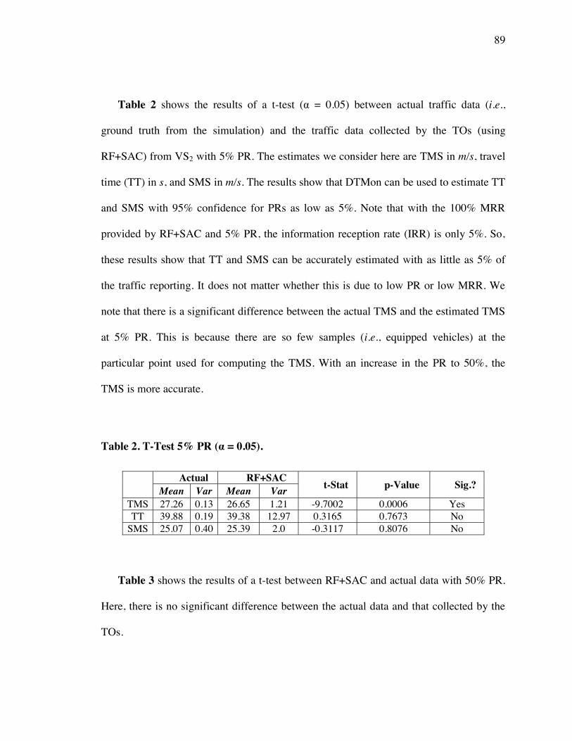
89
Table 2 shows the results of a t-test ( = 0.05) between actual traffic data (i.e.,
ground truth from the simulation) and the traffic data collected by the TOs (using
RF+SAC) from VS2 with 5% PR. The estimates we consider here are TMS in m/s, travel
time (TT) in s, and SMS in m/s. The results show that DTMon can be used to estimate TT
and SMS with 95% confidence for PRs as low as 5%. Note that with the 100% MRR
provided by RF+SAC and 5% PR, the information reception rate (IRR) is only 5%. So,
these results show that TT and SMS can be accurately estimated with as little as 5% of
the traffic reporting. It does not matter whether this is due to low PR or low MRR. We
note that there is a significant difference between the actual TMS and the estimated TMS
at 5% PR. This is because there are so few samples (i.e., equipped vehicles) at the
particular point used for computing the TMS. With an increase in the PR to 50%, the
TMS is more accurate.
Table 2. T-Test 5% PR ( = 0.05).
Table 3 shows the results of a t-test between RF+SAC and actual data with 50% PR.
Here, there is no significant difference between the actual data and that collected by the
TOs.
Actual RF+SAC t-Stat p-Value Sig.? Mean Var Mean Var TMS 27.26 0.13 26.65 1.21 -9.7002 0.0006 Yes TT 39.88 0.19 39.38 12.97 0.3165 0.7673 No
SMS 25.07 0.40 25.39 2.0 -0.3117 0.8076 No

90
Table 3. T-test 50% PR ( = 0.05).
Actual RF+SAC t-Stat p-Value Sig.? Mean Var Mean Var TMS 26.34 0.23 27.08 0.67 1.0689 0.2005 No TT 40.62 0.28 38.84 0.05 0.4025 0.5127 No
SMS 24.62 0.03 25.74 0.01 2.2064 0.3911 No
Table 4. T-test 50% PR ( = 0.05).
RF RF+SAC t-Stat p-Value Sig.? Mean Var Mean Var
TMS 27.45 0.41 27.08 0.67 2.9473 0.2082 No TT 39.17 1.35 38.84 0.05 0.5075 0.7010 No
SMS 25.52 2.01 25.74 0.01 0.0521 0.9668 No
Since the forwarding method can affect the number of samples received by the TOs,
we look at how well the data obtained using RF compared to RF+SAC with 50% PR. We
show the results of the t-test in Table 4. There is no significant difference between the
data collected with RF+SAC and with RF. So with a higher PR, TMCs could use
forwarding-only techniques to lower the message delay, while still receiving high quality
estimates.
4.3. TRAFFIC WITH TRANSIENT FLOW
Our goal in this section is to evaluate the performance of the DTMon to measure travel
times and speeds in transient flow traffic caused by non-recurring congestion. Because
the coverage area of a single TO is limited and transient traffic conditions can cause
periods of network disconnectivity, there is a need for multiple TOs in areas that are
91
prone to experiencing non-recurring congestion events. When multiple TOs are used,
message delay and latency may affect the quality of data that can be accurately gathered.
In addition, it is important to carefully assign measurement points in transient traffic as
the conditions can change quickly. We show how DTMon can allow for the dynamic
creation of new measurement points (VS) and the movement of existing VS.
4.3.1. Congestion
There are two types of traffic congestion. Recurring congestion occurs regularly at the
same locations on the roadway system at about the same time every day. Non-recurring
congestion occurs when a crash or other unusual event (such as a construction zone,
merging traffic, or severe weather) causes a reduction in the traffic-carrying capacity.
Detecting recurring congestion is not a critical monitoring process and requires a long-
term overview (i.e., weekly, monthly, or annual) of a large archive of collected traffic
data, estimated metrics, and structural features of the roads (e.g., capacity) in addition to
extra data-mining to detect the recurrence of similar patterns, all of which can be done
offline. Detecting and monitoring non-recurring congestion, on the other hand, is an
important function of TMCs. Extended periods of non-recurring congestion may require
immediate action, including notifying emergency personnel, highway patrols, or even
changing traffic light timings on surface streets to handle the extra capacity from diverted
highway vehicles.
4.3.2. Latency
In DTMon, tasks can include the locations of multiple TOs. This adds the ability for
messages to be stored and be dropped off at the next available TO during the travel (using

92
RF+SAC). This will reduce the number of messages lost due to unsuccessful forwarding.
In addition to covering a wider area, the use of multiple TOs can improve the message
delivery mechanism. The delay between a vehicle passing a VS and delivering the report
to a TO may be reduced in some instances. Furthermore, generated reports and traffic
warnings by TOs can be spread faster and more reliably in the region.
As described in Sections 3.2.3.2 and 4.2.2.2, message delay is the delay from when a
message was generated to when it was received by a TO. Since vehicles timestamp all
reports, the receiving TO can calculate the message delay for each message. When
messages are delivered to multiple TOs in a region, there is additional processing delay
associated with sending the message to the central TMC and having that data aggregated
with previously received data. We use the term latency for the total time from when a
message was generated to when it is ready to be used in analysis. In a single-TO system,
the latency is the same as the message delay. TMCs often aggregate data and use specific
averaging intervals (e.g., 1 min, 5 min) when reporting traffic conditions. Latency is
important if it rises to higher than the averaging interval. In this case, some late-arriving
data may not be included in the estimate.
4.3.3. Dynamically Defined Virtual Strips
The location of VS can be re-defined and modified by a TO at any time. A TO can divide
the roadway into several virtual segments. The size of the segments can vary by
relocating the VS. Also, additional VS can be defined inside any desired virtual segment.
This allows the TO receive more traffic information by defining additional points of
interest on the road without the cost of using additional TOs. Currently, achieving this

93
would require the installment of numerous sensors and detectors along the road. In AVL
and WLT systems, this would require a significant increase in the sampling rate to
maintain the desired level of accuracy [77].
Congestion can produce a transition in traffic flow which cannot be detected by
probe-based systems when the PR is not high. We show that the transition in the flow rate
can produce a transition in travel time and SMS, which can be detected by DTMon. The
travel time algorithms proposed by Sethi et al. [78] and Sermons [79] utilize both the
travel time and average speed measures of the congested segment and the adjacent
segment. DTMon using dynamically defined strips/segments can satisfy this data
requirement. Two variables, travel time and speed, are compared to historical averages
for each segment to infer if congestion occurs on this segment. It was found by Sethi that
traffic measures for the congested segment were most useful for detecting congestion
located in the downstream portion of the segment, while traffic measures for the next
upstream segment worked well for detecting congestion occurring in the upstream or
middle portion of the segment. The segment in the upstream portion that shows no
significant change in traffic measures is inferred to be the end-of-the-queue.
Identifying the end-of-the-queue is important for traffic engineers as this is the place
where most secondary incidents occur. The primary incident is the cause of the
congestion, but secondary incidents tend to occur at the point where the speed transition
is the sharpest. Traffic engineers would like to be able to identify these locations so that
approaching drivers can be warned in advance, potentially avoiding the secondary
incidents. We explain how DTMon can be used to determine the end of the queue in

94
congested traffic in Section 4.3.5.5. We show that transitions in travel times and speeds
detected by DTMon are two major factors in inferring the possibility of the congestion on
the roadway.
4.3.4. Methodology
We again use our VANET modules [34] to examine DTMon�’s ability to collect high-
quality traffic data, especially travel times and SMS, in transient flow traffic (i.e., non-
recurring congestion).
Figure 25. Location of TOs and virtual strips (not to scale).
As shown in Figure 25, TO1 is located 1 km away from the entrance of a bi-
directional four-lane highway. TO5 is located 5 km away from the beginning of the
highway as an optional secondary TO for the cases when RF+SAC is used. The vehicles
enter the highway with a medium flow rate (average 1800 veh/h) to simulate slightly
sparse traffic [31, 33] where the possibility of message reception by TOs is much lower
than in dense traffic. Trucks, which keep a larger inter-vehicle spacing and have slower

95
acceleration and deceleration than cars, comprise 20% of the vehicles. The desired speed
of all vehicles is 65±5 mph (29±2.2 m/s).
We induce congestion by stopping a vehicle in the first lane, 1.5 km away from the
entrance, between VS1 and VS2, 5 minutes after the simulation has started. The stopped
vehicle is outside the communication range (300 m) of TO1 and is relatively far from
TO5. The vehicle will remain stopped for 5 minutes, then the vehicle will start moving,
allowing traffic flow to gradually return to normal. During the stopped phase, following
vehicles will slow and try to change lanes around the stopped vehicle. This causes traffic
congestion in both lanes. We have observed through experimentation that 5 minutes is
long enough to create a transient flow. Note that congestion could have occurred at any
point on the road, and virtual strips can be defined dynamically by TOs. We examine
advantage of dynamically defined virtual strips in Section 4.3.5.5. At this point, we
named only those VS that surround the starting point of the congestion.
The performance of DTMon in monitoring traffic data is compared with the actual
simulation status (ground truth) at VS2 (2 km away from the highway entrance and 0.5 km
from the stopped vehicle). To compare our system with AVL, we assume that some
percentage of the trucks are able to periodically communicate directly to an operating
center to report their current status. In this comparison, we assume that AVL is used only
by trucks, which we note have slower speeds, acceleration, deceleration than cars. For
comparison with fixed point sensors and detectors (e.g., ILDs or microwave radar
sensors), we use actual simulation data sampled from VS1 and VS2. We execute 10 runs
of the simulation (20 min each) for each experiment. We test PRs of 5, 10, 25, 50, and

96
100%. Travel times, speeds, delays, and message reception rated are measured by TOs.
We compare the results for each scenario using t-test with 0.05 and 95% confidence.
4.3.5. Evaluation
There are several factors that can affect the quality of data gathered by DTMon. The first
factor is the percentage of equipped vehicles, or the market penetration rate (PR). Second,
we are concerned with the amount of information (i.e., location, speed, time) that is
received from vehicles. Third, we must consider how quickly and in what manner the
information is received. Methods that can collect more information from vehicles (higher
MRR and IRR) with less latency are preferred in up-to-date traffic monitoring.
4.3.5.1. MRR and IRR using RF or RF+SAC
For strips within transmission range of TO1 (e.g., VS1), the message reception rate
(MRR) is 100% and the information reception rate (IRR) equals the market penetration
rate (PR). For farther strips where message delivery is required, the MRR using regular
forwarding (RF) varies according to the distance from the TO and the PR. When
RF+SAC is used, only PR affects the MRR.
Table 5 shows the MRR for RF, RF using traffic in the opposite direction, and
RF+SAC for different penetration rates. With low PR, no messages were able to be
forwarded using RF. Even using traffic in the opposite direction does not improve the
MRR. In 25% PR, TO1 receives only 5.71% of messages (only 1.43% of total
information) from VS2. Only RF+SAC was able to deliver messages with full MRR. In
medium PR (e.g., around 50%), RF can deliver almost half of the messages although the
IRR still remains below 30%. Using traffic in opposite direction only improved MRR by

97
7%. In 100% PR, TO1 misses about 20% of messages when RF alone is used (due to
medium traffic flow rate and high inter-vehicle spacing). Using traffic in the opposite
direction for delivery improves the MRR by 15%.
Table 5. MRR for different penetration rates.
PR Actual RF RF+w/opp RF+SAC 5% 100 0.00 0.00 100
25% 100 5.71 5.71 100 50% 100 52.03 56.20 100 100% 100 79.50 91.01 100
Table 6 shows the corresponding IRR. Note that, having low IRR in low penetration
rates means that the system cannot estimate traffic flow rate or density. For example,
DTMon in 25% PR can only count 1.43% (25% with SAC) of vehicles in the traffic, thus
the flow rates estimated by DTMon will be 0.014 (0.25 with SAC) of the actual flow rate
on the road. This is a limitation of any system that does not directly count the physical
presence of vehicles.
Table 6. IRR for different penetration rates.
PR Actual RF RF+w/opp RF+SAC 5% 100 0.00 0.00 5 25% 100 1.43 1.43 25 50% 100 26.01 28.10 50
100% 100 79.50 91.01 100

98
Figure 26 shows the percentage of messages that were forwarded or carried using
RF+SAC in different penetration rates. Even in 100% PR, 20% of messages were carried.
Figure 26 also shows that with 100% PR using RF, in which no messages are carried,
DTMon will count 20% fewer vehicles than actually exist. This is because inter-vehicle
spacing can still be above the DSRC transmission range (300 m) in medium traffic flow.
This is especially true for sections after a point of congestion but before VS2 where the
traffic flow rate decreases and the gap among vehicles increases.
Figure 26. MRR from VS2 using RF+SAC in different PRs.
4.3.5.2. Travel Time and Space Mean Speed
First, we show that ILDs cannot accurately estimate travel times during transient traffic
flow. Next, we investigate how well DTMon is able to measure travel times and SMS
compared to current technologies.

99
Figure 27 shows the travel time in seconds, averaged every 5 minutes, for ILDs along
with the actual (ground truth) travel times. Recall that congestion starts from beginning of
the second interval (t = 5 minutes), reaches its peak at the end of this interval (t = 10
minutes), and starts to release during the third interval (t = 10-15 minutes). Since the
ILDs estimate the travel time as the segment size divided by the averaged traffic spot
speed, they cannot accurately follow the transient nature of the non-recurring congestion
event.
Figure 27. Estimated travel time by ILDs compared to actual (aggregation every 5
minutes).
Probe-based monitoring can perform better than ILDs for measuring travel times and
SMS, so we compare the estimated travel time and SMS during each interval (1 min or 5
min) among data collected using RF, RF+SAC, and with AVL. RFp is RF with a PR of p.

100
In AVL where only trucks are equipped, AVLp is AVL with p percentage of trucks
equipped. For example, AVL25 means 25% of the trucks in traffic are equipped and use
AVL. AVL25 can be compared with RF5 in DTMon since 5% of the total population of
vehicles are equipped and 20% of all vehicles are trucks.
Tables 7 and 8 show the results of a t-test with = 0.05 (95% confidence) for travel
time (in seconds) in four 5-minute intervals, as well as the average travel time and SMS
(in m/s) for the entire 20 minutes with 5% PR. The t-Stat column is the result of the t-test,
showing if the mean of the samples is larger or smaller than the mean of the actual data.
The p-Value column is the probability that the sample and the actual data come from
different distributions. If p-Value is less than (0.05), then the sample population and the
actual population are deemed to have a significant statistical difference.
Table 7. T-test AVL25 and Actual.
Time (min)
Actual AVL25 t-Stat p-Value Sig.? Mean Var Mean Var 0-5 38.55 0.40 43.12 0.03 -1.5326 0.0393 Yes 5-10 119.51 0.46 138.01 0.02 -7.0277 0.0055 Yes
10-15 99.59 0.32 127.86 0.60 -1.8161 0.0018 Yes 15-20 40.62 0.28 42.97 1.10 -2.1121 0.0400 Yes 0-20 74.57 1456.39 87.99 1163.09 -0.8172 0.0360 Yes SMS 13.41 - 11.36 - - - Yes
Travel time and SMS estimated by AVL25 systems have significant differences
compared to the actual data as shown in Table 7. This is because mainly trucks have
lower acceleration and deceleration than cars. Table 8 shows that even in 5% PR,
RF5+SAC provides travel times and SMS with no significant difference from the ground

101
truth. In addition, the eminent change in travel time with a large mean difference
occurring in the second and third intervals shows the possibility of congestion or
transition in traffic flow.
Table 8. T-test RF5+SAC and Actual.
Time (min)
Actual RF5+SAC t-Stat p-Value Sig.? Mean Var Mean Var 0-5 38.55 0.40 40.40 5.19 -0.9700 0.4371 No 5-10 119.51 0.46 113.89 666.13 0.6910 0.0559 No
10-15 99.59 0.32 105.39 902.07 -2.8911 0.0223 Yes 15-20 40.62 0.28 39.38 21.68 0.0060 0.9577 No 0-20 74.57 1456.39 69.77 1025.95 0.0773 0.9391 No SMS 13.41 - 14.33 - - - No
Figure 28. Average travel time (aggregation every 5 minutes).

102
Figure 28 shows the travel times for actual, AVL25, and RF+SAC5. Note that RF5 has
0.0 MRR and therefore no travel time can be estimated. As indicated in Tables 7 and 8,
RF+SAC5 can produce travel times much closer to the actual traffic status than AVL25.
We note that the performance of AVL in estimating travel times and speeds could be
closer to that of RF+SAC if other types of vehicles (e.g., sedans) were also equipped with
AVL devices. In such cases, AVL (in the best case and avoiding the inaccuracy in
sampled data and interpolation by AVL) may perform as accurately as RF+SAC.
Table 9. T-test AVL100 and Actual.
Time (min)
Actual AVL100 t-Stat p-Value Sig.? Mean Var Mean Var 0-5 38.55 0.40 44.95 0.01 -15.8148 0.0402 Yes 5-10 119.51 0.46 144.98 0.0007 -54.8502 0.0116 Yes
10-15 99.59 0.32 139.86 0.03 -153.0912 0.0041 Yes 15-20 40.62 0.28 44.79 0.08 -23.6415 0.0269 Yes 0-20 74.57 1456.39 93.64 2722.33 -3.4170 0.0111 Yes SMS 13.41 - 10.67 - - - Yes
Table 9 shows that even AVL100 provides a significantly different estimation of travel
time and SMS compared with the actual status of the highway. Table 10 shows that RF50
(and by extension, RF+SAC50) can provide high quality estimation of travel time and
SMS that is not significantly different than the actual traffic conditions. The addition of
SAC to RF will only add to the data quality because even more data can be delivered than
with RF alone. Table 11 shows the comparison between RF50 and RF+SAC50. Some of
the messages with RF+SAC may have higher message delay, but as long as the delay is
less than the aggregation interval, the data can be used in the traffic analysis.

103
Table 10. T-test RF50 and Actual.
Time (min)
Actual RF50 t-Stat p-Value Sig.? Mean Var Mean Var 0-5 38.55 0.40 39.00 2.01 -0.3117 0.80761 No 5-10 119.51 0.46 115.78 9.85 2.1514 0.2769 No
10-15 99.59 0.32 123.55 367.38 -1.7165 0.3358 No 15-20 40.62 0.28 39.17 1.35 3.2641 0.1892 No 0-20 74.57 1456.39 79.37 1918.00 -0.9630 0.3676 No SMS 13.41 - 12.59 - - - No
Table 11. T-test RF50+SAC and RF50.
Time (min)
RF50 RF50+SAC t-Stat p-Value Sig.? Mean Var Mean Var 0-5 39.00 2.01 38.94 0.01 0.0521 0.9668 No 5-10 115.78 9.85 116.72 0.15 -0.4858 0.7120 No
10-15 123.55 367.38 97.92 0.01 1.8805 0.3111 No 15-20 39.17 1.35 38.84 0.05 0.5075 0.7010 No 0-20 79.37 1918.00 73.10 1388.43 1.2612 0.2476 No SMS 12.59 - 13.67 - - - No
Figure 29. Travel time in 50% PR (aggregation every 5 minutes).

104
Figure 30. SMS in 50% PR (aggregation every 5 minutes).
Figures 29 and 30 show the estimated travel time and SMS, respectively, in 50% PR.
Because of the 100% MRR that RF+SAC provides, DTMon is able to track the actual
traffic status even during the transient flow periods.
Figure 31. SMS in 50% PR (aggregation every minute).

105
Figure 31 shows the trend in SMS when the aggregation interval is 1 minute. This
indicates that transitions in traffic flow rate can affect travel times and speeds. Even at
this level of aggregation, RF+SAC can track the actual status closely.
Table 12 summarizes the comparison of DTMon with conventional sensors and
detectors currently in use as well as other probe vehicle-based systems, such as AVL.
Note that WLT system performance is very similar to AVL except that WLT has also
issues with accurately detecting the location and timing of vehicles at a specific point.
Table 12. Comparison of DTMon with other technologies.
Good Estimate? Sensors and Detectors AVL (using trucks) DTMon
Travel Time Not Available Overestimate Yes SMS Not Available Underestimate Yes
As mentioned earlier, point-based sensors and detectors cannot directly measure
travel times. AVL systems are typically installed in commercial trucks (or taxis, etc.),
which have different characteristics than the majority of traffic (slower
acceleration/deceleration, larger inter-vehicle gaps, resulting in longer travel times).
4.3.5.3. Latency (Message Delay)
Sensors and detectors sense vehicles instantly. Their collected data are usually transferred
to a TMC periodically via cable or wireless communication with some amount of latency.
The aggregation usually happens every 5 minutes [14, 16]. In AVL systems, vehicles�’
location and speed are probed periodically with negligible delay but these locations and
speeds must be interpolated for a desired location and specific point on the road. For
example, a vehicle with maximum speed 30 m/s may be probed anywhere in the range of

106
150 meters around VS2 when the sampling period is every 5 seconds (which is a high
rate). In the best case, a vehicle�’s location is probed when it is exactly passing VS2 at
probe time. With a lower sampling rate, this offset increases.
Latency in DTMon varies depending upon several factors. The variation in the delay
depends on the method of message delivery. For example, RF adds very small delay (in
terms of milliseconds), while store-and-carry adds some travel time to the carried
messages. In the previous section, we showed that TOs are capable of collecting and
estimating high quality travel times and speeds as well as their trends even in traffic with
transient flow rate and with various market penetration rates.
Figure 32. Message delay.
Figure 32 shows the message delay when RF+SAC is used with different PR. Recall
from Table 5, in 5% PR, the MRR (of messages sent from VS2 to TO1) is zero when RF

107
is used and only RF+SAC could deliver the messages. This increases the message delay
by the average travel time from VS2 to TO5. In medium PR like 50%, almost half of the
messages could be forwarded to TO1, with an average message delay of 7 ms. The rest of
the messages are carried to TO5. Congestion during the second and third interval
(between 5-10 minutes) also adds additional delay to the messages that are carried. In
high PR like 100%, more messages are forwarded (80%) than carried (20%) and the
average message delay becomes lower.
Message delay can be a factor in selecting the method of message delivery. In Tables
10 and 11 we showed that in 50% PR and higher, RF and RF+SAC can provide high
quality estimation of traffic speed and travel time and can also sense transition and trends
in traffic flow based on travel time and SMS with 95% confidence. The advantage of
using RF alone is that we can use a single TO instead of multiple TOs to cover the area,
resulting in a latency below one second. The disadvantage of RF is a lower IRR
especially for VS far from a TO. In contrast, RF+SAC results in higher IRR, especially in
low PR, but with added latency. This latency can vary according to the traffic conditions
and the distance from TOs.
Message delay can also be used to show how fresh the generated reports are. This
may be crucial in real-time traffic monitoring. For example, aggregation may happen
every minute as shown in Figure 31, but during congestion the message delay was 70
seconds for RF+SAC50 (Figure 32), resulting in deviations from the actual traffic status.

108
4.3.5.4. Count Information
Count-based metrics such as flow rate, volume, and density can only be estimated when
the market penetration is high. Figure 33 shows the computed flow rate by DTMon with
100% PR during each time interval. Only 20% of the traffic are trucks, therefore the
estimated flow rate using AVL is inaccurate. RF100 on average has 79.50% IRR and
missed 21.5% of the vehicles that passed VS2. RF100+SAC collects all messages and
reports the same flow rate as ILDs and the actual traffic status. In 100% PR, RF and
RF+SAC can detect the transition in flow rate as shown in Figure 33. Thus, for high PR
scenarios, DTMon can be a good replacement system for sensor and detectors. In low or
medium PR, DTMon can be used to augment current systems and add important travel
time and SMS data.
Figure 33. Flow rate at VS2 in 100% PR (aggregation every 5 minutes).

109
4.3.5.5. End-of-the-queue Virtual Segment
As we explained in Section 4.3.3, identifying the end-of-the-queue is important for traffic
engineers as this is the place where most secondary incidents occur. The primary incident
is the cause of the congestion, but secondary incidents tend to occur at the point where
the speed transition is the sharpest. Traffic engineers would like to be able to identify
these locations so that approaching drivers can be warned in advance, potentially
avoiding the secondary incidents. We explained the importance of dynamically defined
virtual strips and virtual segments for detecting end-of-the-queue in traffic with
congestion in the previous sections. We showed that the transition in the traffic flow rate
cannot be detected in low PRs, although a transition in the traffic flow rate can produce a
transition in travel time and speed which can be detected using DTMon.
We show an example of detecting an end-of-the-queue using DTMon in this section.
A vehicle breaks down after 600s of simulation (10 min) in the first lane at a location
approximately 3.5 km from the highway entrance, far from TO1 which is located 1 km
away from the highway entrance. The vehicle blocks the first lane of the road in two-lane
highway for a long period (30 min). This causes kilometers of backup and congestion in
the traffic that initially has a flow rate 3600 veh/h and speed 29 m/s. After a total of 40
minutes have passed, the blocking vehicle starts moving in order to release the congestion
for the remaining 20 minutes of the one hour simulation.
During the 30 minutes of blocking, a backup starts to form, and the end of the backup
will move. The end will fall into different virtual strips/segments of 1 km size VS1, VS2,
VS3, VS4 (VS1VS2, VS2VS3, and VS3VS4 respectively) which were predefined by TO1.

110
The virtual strips VS2.5 and VS3.5 will be dynamically defined by TO1 during the
congestion, after the vehicle�’s break-down (and its location) is reported to TO1 (as shown
in Figure 34). TO1 (and TO5 if necessary for low penetration rates) monitor the traffic
speed and travel time for each defined strip and segment. Note that we have shown the
impact of penetration rate, distance, and use of store-and-carry in our previous
experiments. In this experiment, we plan to show how TO1 (with average message delay
of less than1 second where RF is used) can infer the end location of the backup in traffic.
Figure 34. Location of TOs and VS (not to scale).
Figure 35 shows the traffic speed at defined virtual strips when averaged every
minute. The transition in traffic speed at a specific VS can be used to infer that the
backup has passed that VS, since traffic behind that strip has a slower speed. For example
at time 24 min, the backup has not reached VS3 because the monitored traffic speed for
that strip was still high. But at time 26 min, the backup endpoint must have passed VS3
because the traffic passing VS3 reported a very low speed. Figure 35 shows the ability of

111
DTMon to detect the transition in traffic speed, which is one important factor to locate
the end of the queue.
Figure 35. TMS at virtual strips. Traffic stoppage occurs during 10-40 min.
In Figure 36, we show an alternate view of data in Figure 35 to highlight the
movement of the end of the queue. The darker points indicate lower traffic speeds. If the
traffic speed for a VS (e.g., VS2.5 at 2100s) is dark and the traffic speed for the location
ahead is dark too (e.g., VS3 at 2100s), the TO can infer that congestion has reached the
VS. When the points become brighter (e.g., VS3 at 3000s), it means that the speeds are
increasing, therefore the TO can infer that the congestion must have been released at VS3.
Figure 36 shows the ability of DTMon to detect the transition in traffic at various points
on the road and at any dynamically defined virtual strip. DTMon can compare these

112
transitions in speed at any two consecutive virtual strips. This is helpful to locate the end
of the back up or the release in the back up.
Figure 36. Time, Space, and Speed.
Figure 37. Travel time for defined virtual segments.

113
Figure 37 shows the travel time averaged every minute at the dynamically defined
virtual strips. Transitions in travel time in a specific virtual segment can be used to infer
whether the backup has reached that virtual segment or not. For example, travel time in
segment VS2VS3 starts to increase after 25 min, showing that the backup has reached this
segment and has started to expand toward the farther strips. The TO can dynamically
define VS2.5 define in this segment to monitor whether the backup has reached the upper
section (VS2.5VS3) or lower section (VS2VS2.5) of the segment VS2VS3. For example, the
traffic speed at VS2.5 (see Figures 35 and 36 ) has sharply decreased after 35 min, and the
travel time for the segment VS2V2.5 has increased, showing that the backup must have
reached into VS2VS2.5, the lower section of the segment VS2VS3. In contrast, the end-of-
the-queue must have been inside the upper section between 25 min to 35 min. Overall,
Figures 35, 36, and 37 show the advantage of dynamically defined virtual strips in
DTMon, and DTMon�’s ability to infer the location of the end of the queue during
congestion.
4.4. ESTIMATING MARKET PENETRATION RATE
In the previous sections, we have shown that DTMon can be used to estimate high-
quality travel times and speeds with relatively low PRs. But, DTMon, as with any probe-
based system, can only estimate high-quality flow rates and density with high PRs. As the
quality of flow rate and density measurements are proportional to the PR, the level of PR
needed for high-quality estimates depends on the acceptable error level. It is possible to
augment DTMon with current technologies such as sensors and detectors (i.e., MRS or
ILDs) and use the count information data collected by these technologies fused with data
114
collected by TOs. As a result, data collected by the TOs are augmented by data gathered
from sensors and detectors for the same virtual strip (same point of interest on the road).
This gives a TO the ability to estimate the PR by observing the total number of equipped
and unequipped vehicles which pass virtual strips in the range of the TO. In this case, the
total number of vehicles (equipped + unequipped) is collected by sensors and the total
number of equipped vehicles is collected by the TO. Once the PR is estimated, we can
apply it to density and flow rate measurements to increase the quality of those estimates.
We expect that the PR in an area will change very slowly over time, so this estimation
could be done once and used to augment DTMon�’s density and flow rate estimates for
several months.
4.5. USING STATISTICAL SAMPLING IN DTMON
There are statistical methods (e.g., Sample Size with Acceptable Absolute Precision for
Finite Populations [80]) that can be used to determine how many samples (reports) are
required to be received by a TO to maintain a desired level of accuracy and confidence in
the traffic estimates. These methods require the input of acceptable variance, acceptable
significance level, and acceptable absolute error and output the required sample size.
In DTMon, the traffic conditions (including the PR) play a major role in the number
of messages that a TO successfully receives. Even in 100% PR, the TO may not have a
high message reception rate from virtual strips that are out of its range, therefore the TO
will task all passing equipped vehicles in order to be sure it can keep the message
reception rate high from farther strips. This will help to keep the message reception rate
at its maximum in any traffic condition with various penetration rates. Also, the accuracy

115
of estimated metrics will remain at its maximum. We do not consider the problem of
sampling and distributing tasks by TOs to a smaller population of equipped vehicles. The
goal of traffic monitoring by the TMC is to collect and archive all possible data for
accurate record-keeping and archiving. As the goal of DTMon is to support this data
collection, we strive to collect all possible data. This is feasible because there is not much
overhead in DTMon, as mentioned in Chapter 3 (Sections 3.1.3 and 3.1.5.3). Reports
where sampling could be employed, such as travel times and speeds, can be piggybacked
on flow rate and density (volume) reports, where the data from the maximum number of
vehicles is required for high-quality estimates.
4.6. SUMMARY
We analyzed the ability of DTMon to provide high-quality traffic data in free-flow traffic
with low to medium market penetration rates. We showed how MRR and IRR were
affected by the market penetration rate, traffic speed, traffic flow rate, and distance of the
measurement point (VS) from the TO. The IRR directly impacts the quality of certain
traffic data. We evaluated different methods of delivering messages to improve the IRR
and showed that an improvement in the message reception rate can have the cost of
increased message delay. But, regardless of the method of message delivery, we showed
that DTMon can collect high-quality travel time and speed data in free-flow traffic where
the possibility of receiving messages from just a few vehicles exists.
In general, average speed, travel time, SMS are not affected by missing messages
(unless all are lost or failed to be delivered). The amount of difference in calculated
averages for speed (TMS and SMS) and travel time are negligible. This shows that with

116
a lower penetration rate and a higher miss rate, these averages can still be good
estimations for actual traffic speed and travel time. On the other hand, the estimate of
traffic flow rate, volume, and density are affected by information reception rate. DTMon
can only provide good estimate of count information in traffic with high penetration rates.
Overall, store-and-carry can always deliver the data from strips when multiple TOs
are deployed, especially for low market penetration rates. This may add cost to system as
well as latency in delivering messages. DTR can only improve the system when the
market penetration rate is medium or high, and it will perform to equal RF in low market
penetration rates or with low density traffic. Nevertheless, TMS, SMS, and travel time
can be estimated even with few samples in free flow traffic.
We also showed that DTMon can provide high quality travel time and SMS data in
transient flow traffic, such as that caused by non-recurring congestion. Currently-
deployed sensors and detectors can only estimate these metrics, and with transient flow
traffic, the estimates are often far off from reality. With low market penetration rates,
DTMon�’s measurements may incur some delay caused by vehicles having to carry their
data to a nearby TO. But, even in these situations, DTMon can be used to augment
current fixed point sensors and detectors. With high market penetration rates, DTMon
could replace these sensors and detectors altogether.
In addition to providing up-to-date travel statistics, DTMon can be used to detect
transitions in traffic flow using travel time and speed measurements gathered from
dynamically defined virtual strips. We showed the advantage of using dynamically
defined virtual strips in DTMon and that DTMon can detect end of the queue by

117
monitoring traffic speed and travel time and their transitions from various dynamic points
on the road.
We have shown that DTMon provides better performance than AVL systems in
monitoring these metrics. The decision regarding which of DTMon�’s message delivery
methods to use depends on the market penetration rate, message delay, and acceptable
latency.

118
CHAPTER 5
CONCLUSION AND FUTURE WORK
In this dissertation we introduced DTMon, a framework for monitoring traffic data. The
main components of the DTMon are task organizers, virtual strips, and equipped
vehicles. Task organizers (TOs) are roadside units that can communicate with equipped
vehicles and with a traffic management center (TMC). These TOs can be programmed by
the TMC to task vehicles with performing traffic measurements over various sections of
the roadway. Virtual strips (VS) are the measurement points for TOs. VS can be changed
dynamically and placed anywhere within several kilometers of the TO. This is a vast
improvement over current technology, where specific measurement points must be
decided in advance and hardware installed in those locations. DTMon can be used in both
rural and urban areas with very little infrastructure. We have shown that in medium to
high density traffic, a single TO can be used to collect data over several kilometers of
roadway. The installation of an additional TO past the desired monitoring points allows
for the use of store-and-carry techniques, which would improve DTMon�’s performance in
low density traffic. This system presents a clear advantage over current point-based
monitoring systems in that it can collect highly-desired travel time and speed metrics. In
addition, the VS measurement points can be dynamically defined based on changing
traffic conditions.
We analyzed the ability of DTMon to provide high-quality traffic data in free-flow
traffic with low to medium market penetration rates. We introduced the information

119
reception rate (IRR) and showed how it was affected by the market penetration rate (PR),
traffic speed, traffic flow rate, and distance of the measurement point (VS) from the TO.
The IRR directly impacts the quality of certain traffic data. We evaluated different
methods of delivering messages to improve the IRR and showed that an improvement in
the message reception rate can have the cost of increased message delay. But, regardless
of the method of message delivery, we showed that DTMon can collect high-quality
travel time and speed data in free-flow traffic where the possibility of receiving messages
from just a few vehicles exists.
We showed that DTMon can provide high quality travel time and SMS data in
transient flow traffic, such as that caused by non-recurring congestion. Currently-
deployed sensors and detectors can only estimate these metrics, and with transient flow
traffic, the estimates are often far off from reality. With low market penetration rates,
DTMon�’s measurements may incur some delay caused by vehicles having to carry their
data to a nearby TO. But, even in these situations, DTMon can be used to augment
current fixed point sensors and detectors. With high market penetration rates, DTMon
could replace these sensors and detectors altogether. In addition to providing up-to-date
travel statistics, DTMon can be used to detect transitions in traffic flow using travel time
and speed measurements gathered from dynamically-defined virtual strips. We showed
that DTMon is able to detect end of the queue locations during congestion using
dynamically-defined virtual strips and detecting transition in travel times and speeds. We
have shown that DTMon provides better performance than Automatic Vehicle Location
(AVL) systems in monitoring these metrics. The decision regarding which of DTMon�’s
120
message delivery methods relies on the market penetration rate, message delay, and
acceptable latency.
In Appendix A, we described the first implementation of a vehicular mobility model
integrated with the networking functions in ns-3. The integrated VANET simulator that
include both mobility and network models and allowed us to evaluate the performance of
DTMon in comparison with the rival technologies and over various traffic conditions
(e.g., free flow traffic, traffic with congestion, etc.).
The summary of this dissertation is as follows:
DTMon is a probe vehicle-based system that uses spatial sampling to
dynamically monitor traffic data. DTMon has two major components:
o Task Organizers
o Virtual strips
DTMon can provide high quality estimates of travel time and speed.
DTMon can provide high quality estimates of flow rate and density in higher
penetration rates.
Hybrid message delivery improves information reception rate with the cost
of increased latency as an option for low penetration rates.
o RF and RF+SAC have similar performance in higher penetration rates
o Using RF+SAC is an improving option in low penetration rates
DTMon can detect transitions in traffic flow using estimated travel time and
speed.

121
DTMon can detect end of queue situations in congested traffic via
dynamically-defined virtual strips and transition detection using travel time
and speed.
DTMon can augment current technologies and systems in monitoring
important traffic data.
We contributed the first implementation of a vehicular mobility model
integrated with the networking functions in ns-3.
o Full user control for studying a wide variety of scenarios in
VANETs using realistic mobility and network models
o Customization of almost all aspects of the simulation
o Settings and functions for wireless communication
o Manually and automatically creation of scenarios
o Allowing for feedback
5.1. CONTRIBUTIONS
The contributions of this dissertation are as follows:
1. A method for using probe vehicles to perform spatial sampling of traffic
conditions �– Probe vehicles can provide real-time measurements of speed and
travel time. Using spatial sampling allows for these measurements to be made at
specific locations of interest on the roadway. This avoids the need for
interpolation and estimation that is required when temporal sampling of probe
vehicles is performed.

122
2. An analysis of the factors that can impact the quality of monitored traffic data
when using vehicular networks �– These factors are market penetration rate, traffic
conditions, communication range, distance between communicating entities,
methods of message delivery, message reception rate, and message delay. We
have performed an analysis of these factors and how each contributes to the
quality of traffic data that can be reported. We note that both traffic conditions
and market penetration rate affect the distance between communicating entities.
3. An evaluation of the impact of different methods of message delivery on the
quality of traffic data that can be gathered by vehicular networks �– We compared
four different message delivery methods (regular forwarding, dynamic
transmission range, store-and-carry, and a hybrid approach) by measuring
message reception rate and message delay in different traffic conditions and
different market penetration rates. We found that a hybrid approach (regular
forwarding coupled with store-and-carry and using vehicles traveling in the
opposite direction) can significantly improve the performance of DTMon in
poorly connected traffic conditions. We also showed that when the market
penetration rate is high, the message delay can be reduced significantly.
4. An evaluation of the effectiveness of DTMon as compared with current
technologies such as inductive loop detectors (ILD) and automatic vehicle
location (AVL) �– We show that DTMon can be used to report travel times that are
not statistically different from the actual travel times. In comparison, we show

123
that technologies such as ILD cannot measure travel times with this level of
accuracy.
5. A demonstration of the usefulness of DTMon�’s monitoring approach for
monitoring congested traffic conditions �– We have shown the ability of DTMon
to allow a TMC to dynamically place additional monitoring points (virtual strips)
in locations where congestion is building up. This allows the TMC to detect
transitions in traffic flow using speeds and travel times, without having to rely on
flow rate information. We have shown that DTMon can be used to detect and
track the end-of-the-queue in traffic with congestion.
6. Highway mobility modules for the ns-3 network simulator �– We have contributed
the first highway mobility modules designed to produce realistic vehicle mobility
and communications in ns-3. The mobility model has been validated against the
well-known vehicular mobility models, and the networking components use ns-3,
which has been validated against wireless models. These modules have been
released to the ns-3 community and are now being used by other researchers
around the world.
5.2. FUTURE WORK
Our future work is to continue studying the design of traffic monitoring systems that
could be deployed in different configurations based on roadway topology and traffic
conditions. As we have seen for some types of data, the market penetration rate affects
the quality of data gathered. We have investigated deploying multiple RSUs (e.g., TOs)
in a region and using oncoming traffic to help bridge gaps in connectivity. But, future
124
work may require an investigation of methods for processing collected data from mobile
nodes (e.g., cell phones) or from other sources. This opens various avenues of research,
including communication protocols, wireless characteristics of vehicular (or mobile or
sensor) networks, security, packet delivery and routing algorithms, standardization, real-
time data-mining, and simulation/modeling. In addition to the research on these types of
networks, this work can motivate new directions on the design of appropriate operating
systems and applications of the required devices. These devices may be static or mobile
and may be servers or clients of traffic data. Low cost, high performance data mining
techniques (usually bound with data sources, search engines, and maps) must be
investigated.
We will further investigate the use of dynamically-defined virtual strips and TOs in
DTMon to evaluate the performance of our proposed framework in urban area
specifically where TOs are deployed at intersections. Therefore, we have plans to extend
our implementation of VANET simulation modules for urban areas (e.g., intersections)
and add the ability to read in and use detailed maps instead of a single straight highway.
We also have plans to implement and develop the most recent WAVE/DSRC standard in
ns-3. This will allow users to simulate up-to-date wireless communication for VANETs
based on the standard. We hope that our addition to ns-3 along with our future work will
allow researchers to easily perform high-quality VANET simulations.

125
REFERENCES
[1] Transportation Research Board, Highway Capacity Manual, Washington, D.C..
2010.
[2] A.D. May, �“Traffic Flow Fundamentals,�” Prentice-Hall, Englewood Cliffs, NJ, 1990.
[3] M. Fontaine, �“Traffic Monitoring�” in Vehicular Networks from Theory to Practice,
Ed. S. Olariu, M. C. Weigle, CRC Press, Boca Raton, FL , 2009.
[4] S. Olariu and M.C. Weigle, Vehicular Networks from Theory to Practice, CRC
Press, Boca Raton, FL, 2009.
[5] E. Schoch, F. Kargl, T. Leinmuller, and M. Weber, �“Communication patterns in
VANETs,�” IEEE Communications Magazine, Vol. 46, No. 11, 2008, pp. 119-125.
[6] US DOT. �“Standard Specification for Telecommunications and Information
Exchange Between Roadside and Vehicle Systems - 5 GHz Band Dedicated Short
Range Communications (DSRC) Medium Access Control (MAC) and Physical
Layer (PHY) Specifications,�” ASTM E2213-03, August 2003.
[7] IEEE 1609, Family of Standards for Wireless Access in Vehicular Environments
(WAVE). Available at http://www.standards.its.dot.gov/fact_sheet.asp?f=80 .
[8] D. Jiang and L. Delgrossi, �“IEEE 802.11p: Toward an International Standard in
Wireless Access in Vehicular Environments,�” 68th IEEE Vehicular Technology
Conference (VTC), Calgary, Alberta, 2008.
126
[9] L.A. Klein, Sensor Technologies and Data Requirement for ITS, Artech House,
Boston, 2001.
[10] L.A. Klein, M. Mills, and D. Gibson, Traffic Detector Handbook, 3rd Ed., Vol. 1,
Federal Highway Administration, Washington, D.C., 2006.
[11] Research and Innovative Technology Administration, State Transportation Statistics,
U.S. Department of Transportation, Washington, D.C., 2006.
[12] D. Middleton, D. Jasek, and R. Parker, Evaluation of Some Existing Technologies for
Vehicle Detection, Texas Transportation Institute, College Station, TX, 1999.
[13] S. Hanshaw, �“New�” Data Sources, Paper presented at the North American Traffic
Monitoring Exhibition and Conference, Minneapolis, MN, 2006.
[14] G.L. Ullman, K.N. Balke, W.R. McCasland, and C.L. Dudek, Benefits of Real-Time
Travel Time Information in Houston, Intelligent Transportation: Realizing the
Benefits, ITS America, Houston, TX, 1996.
[15] J. Wright and J. Dahlgren, Using Vehicles Equipped with Toll Tags as Probes for
Providing Travel Times, University of California, Berkeley, CA, 2001.
[16] D.J. Dailey and F.W. Cathey, AVL Equipped Vehicles as Speed Probes, Washington
State Transportation Center, Seattle, WA, 2005.
[17] INRIX, available at http://inrix.com/.

127
[18] Cellular Telephone and Internet Association, Wireless Statistics, available at
http://www.ctia.org/research_statistics/index.cfm/AID/10202, 2006.
[19] Mobile Century/Mobile Millennium project with Nokia. Available at
http://traffic.berkeley.edu.
[20] PATH�’s GEMS project available at http://www.path.berkeley.edu.
[21] P. Mohan and V. Padmanabhan, �“Nericell: Rich Monitoring of Road and Traffic
Condition using Mobile Smartphones,�” The Sixth ACM Conference on Embedded
Networked Sensor Systems, (ACM SenSys 2008), Raleigh, NC, 2008.
[22] A. Thiagarajan, L. Sivalingam, K. LaCurts, S. Toledo, J. Eriksson, S. Madden, and
H. Balakrishnan, �“VTrack: Accurate, Energy-Aware Traffic Delay Estimation Using
Mobile Phones,�” The Seventh ACM Conference on Embedded Networked Sensor
Systems, (ACM SenSys 2009), Berkeley, CA, 2009.
[23] J.C. Herrera, D. Work, J. Ban, R. Herring, Q. Jacobson, and A. Bayen, �“Evaluation
of traffic data obtained via GPS-enabled mobile phones: the Mobile Century
experiment,�” Transportation Research Part C, Berkeley, CA, 2008.
[24] B. Hoh, M. Gruteser, R. Herring, J. Ban, D.Work, J. C. Herrera, and A. Bayen,
�“Virtual trip lines for distributed privacy-preserving traffic monitoring,�” The Sixth
Annual International conference on Mobile Systems, Applications and Services
(MobiSys 2008), Breckenridge, USA, 2008.

128
[25] Connected Vehicle, US Department of Transportation, available at
http://www.its.dot.gov/connected_vehicle/connected_vehicle.htm, 2011.
[26] B. Smith, B. Park, H. Tanikella, and G. Zhang, �“Preparing to Use Vehicle
Infrastructure Integration in Transportation Operations: Phase I,�” Final Contract
Report, Virginia Transportation Research Council (VTRC), 2008. available at
http://www.virginiadot.org/vtrc/main/online_reports/pdf/08-CR1.pdf .
[27] T. Nadeem, S. Dashtinezhad, and C. Liao, �“Traffic View: A Scalable Traffic
Monitoring System,�” Proceeding of the IEEE International Conference. on Mobile
Data Management (MDM), New York, NY, 2004, pp.13-21.
[28] B. Hull, V. Bychkovsky, Y. Zhang, K. Chen, M. Goraczko, A. Miu, E. Shih,
H. Balakrishnan, and S. Madden, �“CarTel: A distributed mobile sensor computing
system,�” Proceeding of the International Conference on Embedded Networked
Sensor Systems (SenSys), New York, NY, 2006.
[29] T. Kitani, T. Shinkawa, N. Shibata, K. Yasumoto, M. Ito, T. Higashino, �“Efficient
VANET-based Traffic Information Sharing using Buses on Regular Routes,�”
Proceeding of the IEEE Vehicular Technology Conference (VTC), Singapore,
Singapore, May 2008, pp. 3031-3036.
[30] A. Krause, E. Horvitz, A. Kansal, and F. Zhao, �“Toward community sensing,�”
Proceedings of ACM/IEEE International Conference on Information Processing in
Sensor Networks (IPSN), St. Louis, MO, 2008.

129
[31] H. Arbabi and M.C. Weigle, �“Using DTMon to Monitor Transient Flow Traffic,�”
Proceedings of the IEEE Vehicular Networking Conference (VNC), Jersey City, NJ,
2010.
[32] H. Arbabi and M.C. Weigle, �“Monitoring Free-Flow Traffic using Vehicular
Networks,�” Proceedings of the IEEE Intelligent Vehicular Communications System
Workshop (IVCS), Las Vegas, NV, 2011.
[33] H. Arbabi and M.C. Weigle, �“Using Vehicular Networks to Collect Common Traffic
Data,�” Proceeding of the ACM International Workshop on Vehicular
Internetworking (VANET), Beijing, China, 2009, pp. 117-118.
[34] H. Arbabi and M. C. Weigle, �“Highway Mobility and Vehicular Ad-Hoc Networks
in ns-3,�” Proceeding of the Winter Simulation Conference, Baltimore, MD, 2010.
[35] A. Halati, H. Lieu, and S. Walker, �“CORSIM-corridor traffic simulation model,�”
Proceedings of the Traffic Congestion and Traffic Safety in the 21st Century
Conference, Heidelberg, Germany, 1997, pp. 570-576.
[36] D. Krajzewicz, M. Bonert, and P. Wagner, The open source traffic simulation
package SUMO, RoboCup 2006 Infrastructure Simulation Competition, Bermen,
Germany, 2006.
[37] PTV America. VISSIM Traffic Simulation Software, available at
http://www.ptvamerica.com/software/ptv-vision/vissim, 2010.

130
[38] M. Fiore, J. Härri, F. Filali, and C. Bonnet, �“VanetMobiSim: Generating realistic
mobility patterns for VANETs,�” Proceedings of ACM VANET, Los Angeles, CA,
2006, pp. 96-97.
[39] L. Breslau, D. Estrin, K. Fall, S. Floyd, J. Heidemann, A. Helmy, P. Huang, S.
McCanne, K. Varadhan, Y. Xu, and H. Yu, �“Advances in Network Simulation, �”
IEEE Computer, Hong Kong, China, 2000, pp. 59-67.
[40] Scalable Network Technologies, QualNet Simulation Software, available at
http://www.scalable-networks.com/products/qualnet, 2010.
[41] OPNET. OPNET Modeler Software, available at
http://www.opnet.com/solutions/network_rd/modeler.html, 2010.
[42] X. Zeng, R. Bagrodia, and M. Gerla, �“GloMoSim: a Library for Parallel Simulation
of Large-scale Wireless Networks,�” Proceedings of the 12th Workshop on Parallel
and Distributed Simulations, Banff, Canada, 1998.
[43] M. Piorkowski, M. Raya, A.L. Lugo, P. Papadimitratos, M. Grossglauser, and J.P.
Hubaux, �“Trans: Realistic joint traffic and network simulator for VANETs,�” ACM
SIGMOBILE Mobile Computing and Communications Review, 2008, pp. 31-33.
[44] F. Karnadi, Z.H. Mo, K. Lan, �“Rapid Generation of Realistic Mobility Models for
VANET,�” Proceedings of IEEE Wireless Communications and Networking
Conference, Kowloon, China, 2007, pp. 2506-2511.

131
[45] K. Ibrahim and M.C. Weigle, �“ASH: Application-aware SWANS with Highway
mobility,�” Proceedings of IEEE INFOCOM Workshop on MObile Networking for
Vehicular Environments (MOVE), Phoenix, AZ, 2008.
[46] C. Gorgorin, V. Gradinescu, R. Diaconescu, and L. Iftode, �“An Integrated Vehicular
and Network Simulator for Vehicular Ad-hoc Networks,�” Proceedings of the 20th
European Simulation and Modelling Conference (ESM), Bonn, Germany, 2006.
[47] A. Hassan, �“VANET Simulation,�” Högskolan i Halmstad, Master Thesis and
Technical Report, Stockholm, Sweden, 2009.
[48] G. Yan, K. Ibrahim, and M.C. Weigle, �“Vehicular Network Simulators,�” Vehicular
Networks: From Theory to Practice, Ed. S. Olariu and M. C. Weigle, Boca Raton,
FL, 2009.
[49] T. Henderson, S. Roy, S. Floyd, and G.F. Riley, �“ns-3 Project Goals,�” Proceedings
of the 2006 workshop on ns-2: the IP network simulator, New York, NY, 2006.
Available at http://www.nsnam.org.
[50] M. Fiore, J. Härri, �“The networking shape of vehicular mobility,�” Proceeding of the
9th ACM international symposium on Mobile ad hoc networking and computing,
Hong Kong, China, 2008, pp. 261-272.
[51] M. Fiore, �“Vehicular Mobility Models,�” Vehicular Networks: From Theory to
Practice, Ed. S. Olariu and M. C. Weigle, Boca Raton, FL, 2009.

132
[52] M. Treiber, A. Hennecke, and D. Helbing, �“Congested Traffic States in Empirical
Observations and Microscopic Simulations,�” Physical Review E, Stuttgart, Vol. 62,
Stuttgart, Germany, 2000, pp. 1805-1824.
[53] M. Treiber and D. Helbing, �“Realistische Mikrosimulation von Straßenverkehr mit
einem einfachen Modell,�” Proceedings of the 16th Symposium Simulationstechnik
(ASIM 2002), Rostock, Germany, 2002, pp. 514-520.
[54] C. Robinson, L. Caminiti, D. Caveney, K. Laberteaux, �“Efficient Coordination and
Transmission of Data for Vehicular Safety Applications,�” Proceeding of ACM
VANET, Los Angeles, CA, 2006.
[55] K. Ibrahim and M. Weigle, �“CASCADE: Cluster-based Accurate Syntactic
Compression of Aggregated Data in VANETs,�” Proceedings of the IEEE
International Workshop on Automotive Networking and Applications (AutoNet), New
Orleans, LA, December 2008.
[56] G. Yan, S. Olariu, and M.C. Weigle, �“Providing Location Security in Vehicular Ad-
hoc Networks,�” IEEE Wireless Communications, Special Issue on On-the-Road
Communications, Vol. 16, No. 6, 2009, pp. 48-55.
[57] C. Harsch, A Festag, P. Papadimitratos, �“Secure Position-Based Routing for
VANETs,�” Proceeding of the IEEE Vehicular Technology Conference (VTC),
Baltimore, MD, 2007, pp. 26-30.

133
[58] P. Papadimitratos, L. Buttyan, T. Holczer, E. Schoch, J. Freudiger, M. Raya, Z. Ma,
F. Kargl, A. Kung, and J.P. Hubaux, �“Secure Vehicular Communication Systems:
Design and Architecture,�” IEEE Wireless Communications Magazine, 2008.
[59] M. Raya and J.P. Hubaux, �“The Security of Vehicular Ad Hoc Networks,�”
Proceeding of the Workshop on the Security of Ad Hoc and Sensor Networks (SASN),
Alexandria, VA, 2005.
[60] H. Fußler, M. Mauve, H. Hartenstein, M. Kasemann, and D. Vollmer, �“Location-
Based Routing for Vehicular Ad-Hoc Networks,�” Proceeding of ACM MobiCom,
Atlanta, GA, 2002.
[61] B. Parno and A. Perrig, �“Challenges in Securing Vehicular Networks,�” Proceeding
of ACM HotNets, Berkeley, CA, 2005.
[62] G. Yan, S. Olariu, and M.C. Weigle, �“Providing VANET Security Through Active
Position Detection,�” Computer Communications: Special Issue on Mobility
Protocols for ITS/VANET, Vol. 31, No. 12, 2008, pp. 2883-2897.
[63] N. Wisitpongphan, O. K. Tonguz, J. S. Parikh, P. Mudalige, F. Bai, and V. Sadekar,
�“Broadcast storm mitigation techniques in vehicular ad hoc networks,�” Wireless
Communications, IEEE, Vol. 14, No. 6, 2007, pp. 84-94.
[64] L. Wischhof, A. Ebner, H. Rohling, M. Lott, and R. Halfmann, �“SOTIS: a self-
organizing traffic information system,�” Proceedings of the 57th IEEE Vehicular
Technology Conference, Jeju, South Korea, 2003.

134
[65] D. Borsetti and J. Gozalvez, �“Infrastructure-Assisted Geo-Routing for Cooperative
Vehicular Networks,�” Proceedings of the IEEE Vehicular Networking Conference
(VNC), Jersey City, NJ, 2010.
[66] F. Kaisser, C. Johnen, and V. Veque, �“Quantitative Model for Evaluate Routing
Protocols in a Vehicular Ad Hoc Networks on Highway,�” Proceedings of the IEEE
Vehicular Networking Conference (VNC), Jersey City, NJ, 2010.
[67] R. Stanica, E. Chaput, and A. Beylot, �“Broadcast Communication in Vehicular Ad-
Hoc Network Safety Applications,�” Proceedings of the IEEE Intelligent Vehicular
Communications System Workshop (IVCS). Las Vegas, NV, 2011.
[68] M. Abuelela, S. Olariu, and I. Stojmenovic, �“OPERA: Opportunistic Packet
Relaying in Disconnected Vehicular Ad Hoc Networks,�” Proceedings of the IEEE
International Conference on Mobile Ad-hoc and Sensor Systems (MASS). Atlanta,
GA, September 2008.
[69] M. Abuelela and S. Olariu, �“SODA: A Smart Opportunistic Data Dissemination
Approach for VANET,�” Proceedings of the 6th International Workshop on
Intelligent Transportation (WIT). Hamburg, Germany, March 2009.
[70] S. Saha, K. Chaudhuri, D. Sanghi, and P. Bhagwat, �“Location Determination of a
Mobile Device Using IEEE 802.11b Access Point Signals,�” Proceedings of IEEE
WCNC, New Orleans, LA, 2003, pp. 1987-1992.
[71] Federal Highway Administration, Traffic Monitoring Guide, Washington, DC, 2001.

135
[72] N. Wisitpongphan, F. Bai, P. Mudalige, V. Sadekar, and O. Tonguz, �“Routing in
Sparse Vehicular Ad Hoc Wireless Networks,�” IEEE Journal on Selected Areas in
Communication, Vol. 25, No. 8, 2007, pp. 1538-1556.
[73] N. Wisitpongphan, O. Tonguz, F. Bai, P. Mudalige, and V. Sadekar, �“On the Routing
Problem in Disconnected Vehicular Networks,�” Proceeding of IEEE INFOCOM,
Anchorage, Alaska, USA, 2007.
[74] G. Yan, S. Olariu, and M.C. Weigle, �“Cross-Layer Location Verification
Enhancement in Vehicular Networks,�” Proceedings of the IEEE Intelligent Vehicles
Symposium, San Diego, CA, 2010.
[75] A. Mahajan, N. Potnis, K. Gopalan, and A. Wang, �“Urban Mobility Models for
VANETs,�” Proceeding of 2nd Workshop on Next Generation Wireless Networks,
Bangalore, India, 2006.
[76] A. K. Saha and D. B. Johnson, �“Modeling mobility for vehicular ad-hoc networks,�”
VANET �’04: Proceedings of the 1st ACM international workshop on Vehicular ad
hoc networks, New York, NY, USA, 2004, pp. 91-92.
[77] A. Faghri and K. Hamad, �“Travel time, speed, and delay analysis using an integrated
GIS/GPS system,�” Canadian Journal of Civil Engineering, Vol. 29, 2002, pp. 325-
328.

136
[78] V. Sethi, N. Bhandari, F. Koppelman, and J. Schofer, �“Arterial Incident Detection
Using Fixed Detector and Probe Vehicle Data,�” Transportation Research Part C-
Emerging Technologies, Vol. 3, 1995, pp. 99-112.
[79] M. W. Sermons and F. S. Koppelman, �“Use of vehicle positioning data for arterial
incident detection,�” Transportation Research Part C-Emerging Technologies, Vol. 4,
1996, pp. 87-96.
[80] Levy P. and S. Lemeshow, �“Sampling of Populations: Methods and Application,�”
Wiley, New York, NY, 1999.
[81] Vehicular Networks (VANETs), Sensor Networks, and Internet Traffic Research in
the Department of Computer Science at Old Dominion University, http://oducs-
networking.blogspot.com/.
[82] M. Treiber, Intelligent Driver Model (IDM), available at traffic-
simulation.de/IDM.html, 2006.
[83] M. Treiber, Minimize Overall Braking decelerations Induced by Lane changes
(MOBIL), available via traffic-simulation.de/MOBIL.html, 2006.
[84] M. Green, �“How Long Does It Take To Stop?,�” Methodological Analysis of Driver
Perception-Brake Times, Transportation Human Factors, 2000, pp. 195-216.
[85] ns-3 Highway Mobility Project, available at http://code.google.com/p/ns-3-highway-
mobility/ .

137
APPENDIX A
SIMULATION MODULES FOR VANETS AND HIGHWAY
MOBILITY IN NS-3
The study of VANETs, and in our case DTMon, requires efficient and accurate
simulation tools. As the mobility of vehicles and driver behavior can be affected by
network messages, these tools must include a vehicle mobility model integrated with a
quality network simulator. We present the first implementation of a well-known vehicle
mobility model to ns-3, the next generation of the popular ns-2 networking simulator.
Vehicle mobility and network communication are integrated through events. User-created
event handlers can send network messages or alter vehicle mobility each time a network
message is received and each time vehicle mobility is updated by the model. To aid in
creating simulations, we have implemented a straight highway model that manages
vehicle mobility, while allowing for various user customizations. We show that the
results of our implementation of the mobility model matches that of the model�’s author
and provide an example of using our implementation in ns-3.
The problem with integrated simulators is that often either the mobility model is
overly simplified or the network model is overly simplified. In order to study important
networking properties of VANETs, a high quality network simulator is essential. We
have chosen to balance these two concerns by taking the latest version of the highly-
regarded network simulator, ns-3 and adding a well-known traffic mobility model in
order to provide an integrated simulator for VANET research. This work [34] has been

138
published and is being used by various researchers and users. ns-3 is a discrete-event
network simulator written in C++, targeted primarily for research and educational use,
and intended as a replacement for the popular ns-2 simulator. ns-3 promises to be a more
efficient and more accurate simulator than its predecessor (especially for wireless
protocols). For this reason, we were interested in using ns-3 to perform our VANET
simulations.
ns-3 provides various mobility models, but none are appropriate to simulate the
mobility of vehicles. The mobility of a node in the mobility models included in ns-3
depends only on the node itself. In realistic vehicular mobility, the mobility of the node
must depend on the surrounding nodes and the conditions on the road. Furthermore, this
node dependency becomes essential when messages in the network can affect the
mobility of the nodes on the roads. For example, the receipt of a safety message may
result in a speed reduction.
We have implemented IDM and the MOBIL lane change model in ns-3 (see Sections
A.1.3 and A.1.4). In addition, we have provided a Highway class to represent a straight
multi-lane, bi-directional roadway. In our simulations, the Highway object is the �“brain�”
of the system and efficiently manages the behavior of vehicles and their mobility on the
road. Each vehicle is a fully-fledged wireless node in ns-3. In this way, vehicles can
move with realistic mobility and communicate with each other to form a VANET. In our
network and mobility combined design, a user can simulate VANETs in highways with
customized road-side and on-board units. Users can create user-defined actions and event

139
handlers to customize simulation scenarios, allowing them to study vehicular traffic,
network traffic, or both.
We explain the main components of our design in Section A.1 and highlight possible
user customizations, such as adding helicopters or embedded highway sensors, in Section
A.2. In Section A.3, we discuss validation of our IDM/MOBIL implementation in ns-3,
and in Section A.4 we discuss an example of our additions to ns-3.
A.1. ARCHITECTURE
Here we describe the components of our design, which consists of five main classes
(Figure 38):
Figure 38. Class diagram of the main components in our design.
1. Vehicle - a mobile node that contains a wireless communications device
2. Obstacle - a Vehicle that has no mobility
3. Model - the IDM car-following mobility model

140
4. LaneChange - the MOBIL lane change model
5. Highway - holds Vehicle and Obstacle objects and uses a Vehicle�’s Model and
LaneChange properties to control its mobility
Highway uses the first four classes to generate the traffic in a highway. Since
vehicular mobility models, and especially car-following models like the one we
implement, need to know the position and mobility of other vehicles, the Highway object
must be used to control the mobility of all vehicles. Users can customize Highway
(including highway length, uni-directional or bi-directional traffic flow, number of lanes,
lane width, and center median width) to create a variety of simulation scenarios.
In the following sections, we will describe each of the classes in order. The source
code, examples, and documentation [34, 81] are available for researchers and developers.
A.1.1. Vehicle
A Vehicle is a mobile node that contains a wireless communications device. A Vehicle
has the following properties:
vehicleID
width - width of the vehicle in meters
length - length of the vehicle in meters
lane - lane number on the highway where the vehicle is located
direction - {-1, 1} (Assume eastbound is 1 and westbound is -1).
position - a vector (x, y, z), where x is the rear position of the vehicle, y is the
center of the vehicle, and z is the altitude of the vehicle above the highway (all
units in meters)
141
velocity - in m/s
acceleration - in m/s2
model - mobility model settings, desired velocity is associated with the mobility
model
lanechange - lane change model settings
In our design, the Highway object is in charge of managing the positions, directions,
and the lane numbers of its vehicles. A Vehicle�’s acceleration and velocity can be set
manually or can be calculated based on the IDM mobility model rules. A Vehicle is able
to change lanes, if necessary and possible, based on the MOBIL lane change model.
Vehicle objects can either be manually created and inserted onto the Highway, or they can
be automatically injected into the Highway.
Since a Vehicle contains a wireless communications device, we can control the
vehicle�’s WiFi capabilities. Vehicles are able to communicate (send/receive) through the
standard ns-3 WiFi channels. The messages, including sent and received packets, and all
related events can be captured by setting the appropriate event handlers to the
implemented callbacks, which are designed and considered for these purposes. A Vehicle
can unicast packets or it can send broadcast messages. The user has full control on how to
schedule the sending process and how to handle the receive callback. There are also
several callbacks for the purpose of tracing the different layers of the network and the
mobility of the vehicle. These help the user create and trace simulation scenarios easily.

142
A.1.2. Obstacle
An Obstacle is a static node that contains a wireless communications device. It is
inherited from the Vehicle class and has all of the capabilities of a Vehicle except that it
cannot be mobile (i.e., velocity = acceleration = model = lanechange = 0). An obstacle
can be used as an barrier to close a lane or to temporarily create stoppages that result in
congestion on the highway. An obstacle can also be used as a roadside unit or other piece
of infrastructure along, but outside of, the highway. If an Obstacle is placed on the
highway, it must have a direction and lane number. Anything that can be done to a
Vehicle object can be done to an Obstacle object (aside from affecting mobility), so in the
rest of this paper we will just use the term Vehicle.
A.1.3. Mobility Model
Model is the class that implements the mobility model for a Vehicle. We have
implemented the Intelligent Driver Model (IDM) in ns-3 based on equations and
parameters developed by Treiber [52, 82]. IDM is a car-following model, meaning that
each vehicle�’s acceleration or deceleration depends upon its own velocity, its desired
velocity, and the position and velocity of the vehicle immediately in front in the same
lane, which Treiber calls the front vehicle.
Each vehicle in IDM has a desired velocity, safety time headway (time needed to
cover a gap between two vehicles, e.g., the �“2 second rule�”), acceleration in free-flow
traffic, comfortable braking deceleration, and desired minimum distance to the front
vehicle. IDM uses these parameters and the current state of the vehicle and front vehicle
to compute the new acceleration. Acceleration is, in turn, used to update the velocity and

143
position of the vehicle. Note that acceleration necessarily decreases towards 0 when the
velocity of the vehicle approaches the desired velocity.
The function CalculateAcceleration in the Model class uses the IDM equations to
calculate and return the new acceleration at each time step. The vehicle�’s new velocity
and position are then adjusted based on this new acceleration.
For customizability, each vehicle can have its own set of IDM parameters. Treiber
suggests different parameter settings for cars and trucks. For example, trucks have a
lower desired velocity and acceleration in free-flow traffic, and longer deceleration gap
than cars. �“Careful�” drivers would have a high safety time headway, and �“pushy�” drivers
would have a low safety time headway, higher desired velocity, higher acceleration, and
higher deceleration.
In our design, we also allow each Vehicle object to have its own IDM parameters. We
have included reasonable default values for cars (the Sedan class) and trucks (the Truck
class). The user can create their own vehicle types with different parameter values for
specific experiments. For example, a user may want to create a mix of careful and pushy
drivers, or include sports cars, police cars, emergency vehicles, and buses, all of which
would have very different mobility characteristics.
A.1.4. Lane Change Model
LaneChange is the class that implements the lane changing model for a Vehicle. We have
implemented the MOBIL lane change model based on equations and parameters
developed by Treiber [53, 83]. Each lane change in this model must satisfy both the
safety criterion and the incentive criterion. The safety criterion states that the lane change

144
must not cause the vehicle that is being changed in front of (the back vehicle) to
decelerate unsafely (faster than a certain threshold). The incentive criterion is satisfied if
the lane-changing vehicle�’s advantage is greater than the other vehicles�’ disadvantages.
Note that although the incentive criterion is usually much easier to satisfy than the safety
criterion, both must hold for the lane change to occur. In addition, the IDM rules still
apply, meaning that the new front vehicle must be a certain distance ahead in order for
the lane change to occur.
To compute the incentive criterion, MOBIL first calculates the lane-changing
vehicle�’s advantage. This is simply the difference between the vehicle�’s current
acceleration and the vehicle�’s new acceleration after the lane change. The goal is to
increase the acceleration, or to reduce the braking deceleration, which are essentially the
same things. The disadvantage to both the back vehicle in the current lane and the back
vehicle in the new lane are considered. Again, this is done by comparing the acceleration
before the lane change with the acceleration after lane change.
To allow for some variability in how aggressive drivers are in deciding when to
change lanes, MOBIL weights the other vehicles�’ disadvantage with a politeness factor,
p. When p 1, the driver is considerate and puts others�’ disadvantages equal to or ahead
of their own advantage. In reality, most drivers are in the 0 < p 0.5 range, where some
weight is given to other drivers�’ disadvantage. If p = 0, the driver is inconsiderate,
discounting the disadvantage to others.
MOBIL also includes a right-lane bias parameter when computing the incentive
criterion. This parameter allows for modeling situations in countries where passing a

145
vehicle on the right is not allowed. The parameter can also be used to allow vehicles to
pass from either side or prevent trucks from travelling in the leftmost lanes.
The function CheckLaneChange in our LaneChange class returns a boolean to
indicate if the lane-change can take place or not. CheckLaneChange uses the MOBIL
equations and suggested parameters along with the statuses of the lane-changing vehicle,
the current front vehicle, the new front vehicle, and the new back vehicle. As with our
IDM implementation, we have included reasonable default values for each of these
parameters. We provide a Considerate driver class and an Inconsiderate driver class. The
user can, of course, create their own driver types with different parameters.
A.1.5. Highway
Highway is the class that holds Vehicles and manages their mobility. We will discuss
Highway�’s physical properties, Vehicle management tasks, and how users can control
vehicles on the highway in order to customize simulations.
A.1.5.1. Physical Properties
Highway represents a straight highway topology and has the following physical
properties:
length �– length of the highway in meters (up to 10,000 m)
number of lanes �– in each direction [1,5]
lane width �– in meters
median gap �– width of the median, in meters
bidirectional �– true if the highway contains two-way traffic, false if the highway
is one-way

146
Figure 39 shows two example highway configurations. Figure 39a is a unidirectional
highway with three lanes, and Figure 39b is a bidirectional highway with four lanes in
each direction.
Figure 39. A small segment of a highway. Cars are represented by small rectangles,
and trucks are represented by larger rectangles. (a) unidirectional highway with
three lanes, (b) bidirectional highway with four lanes in each direction and a
separating median.
A.1.5.2. Vehicle Management
There are several Vehicle management functions that Highway performs. Highway can
automatically create Vehicle objects with certain parameters, automatically insert these
created objects into lanes, and move each Vehicle according to its mobility and lane
change models.
Automatic Creation and Injection of Vehicles: When the AutoInjection parameter of
Highway is true, Vehicle objects will be automatically created and injected onto the

147
highway. For this purpose, Highway creates default mobility models with parameters set
appropriately for the standard car and truck, named SedanModel and TruckModel,
respectively. Highway also creates default lane change models with appropriate
parameters set for cars and trucks. The ratio of cars to trucks that are created is controlled
by the injectionMix parameter. Automatically-created Vehicle objects are provided with
default WiFi Phy/Mac settings appropriate for VANETs.
Highway stores each lane as a list structure. When a Vehicle object is added to
Highway, it is inserted in its proper place according to its lane, direction, and x position.
For auto-injection, there is a minGap parameter that specifies the minimum distance
between two vehicles entering the highway. Newly created Vehicle objects are not
inserted until the x position of the last Vehicle in the lane is at least minGap meters from
the start of the highway. Vehicles are inserted with a negative x position, so that the front
of the vehicle starts at the start of the highway (x = 0) according to user selected flow rate
distribution (i.e. uniform, exponential, normal, log-normal, Poisson) and velocity
distribution (i.e., uniform, exponential, normal, log-normal). Each lane is checked to see
if a Vehicle can be added, in round-robin fashion, starting with the rightmost lane (lane =
0) in the eastbound direction (direction = 1) and ending with the leftmost lane in the
westbound direction (direction = -1, if using bidirectional traffic). Thus, on a
bidirectional highway, vehicles are added to both directions considering the flow rate and
velocity in each direction.
Mobility of Vehicles: Every DeltaT seconds, Highway calls its step function which
updates the position, velocity, and acceleration of each Vehicle according to its mobility

148
model. In this way, vehicles with different mobility characteristics (e.g., trucks,
emergency vehicles) can be represented on the same highway. Vehicles are updated by
lane in round-robin fashion, starting with the Vehicles in the rightmost lane in the
eastbound direction. After the update, if a Vehicle�’s x position is greater than the length
of the Highway, the Vehicle is removed from the lane list. After all Vehicle positions have
been updated, automatic injection of new Vehicles occurs.
The opportunity for each vehicle to change lanes is evaluated every 10 * DeltaT
seconds to prevent unrealistic lane-changing patterns (e.g., vehicles changing lanes
multiple times in less than 1 second). If a vehicle can safely change lanes (according to
the Vehicle�’s MOBIL parameters), Highway removes the Vehicle from the current lane
and adds it to the target lane at the x position specified according to IDM/MOBIL. When
a lane change is allowed, it occurs before mobility is updated, so a Vehicle changing
lanes only has its mobility updated one time in DeltaT seconds.
The best case driver reaction time is 0.7 seconds [84]. Vehicle positions should be
updated more often than the driver reaction time, so we choose 0.1 seconds for the
default value of DeltaT as a tradeoff between efficiency and accuracy. Reducing DeltaT
(i.e., having the step function called more often) will produce a more detailed translation
of the position of the vehicle, but will result in a slower simulation (Figure 40).
Increasing DeltaT (i.e., having the step function called less often) will cause less accuracy
in mobility since each step may result in a larger displacement of the vehicles (Figure
41).

149
Figure 40. The elapsed real time for 1 minute of dense traffic simulation (average
180 vehicle/km).
Figure 41. A vehicle�’s displacement vs. velocity in a single simulation step with
different DeltaT values.

150
User Control of Vehicles: To allow for feedback between the network and the mobility
model, there must be a way for the user�’s application code to interact with individual
Vehicle objects. Highway allows the user to access any Vehicle object through its
VehicleID using FindVehicle(). The user can then use this object to change any of the
Vehicle�’s parameters. In addition, Highway provides FindVehiclesInRange() which
returns a list of all Vehicle objects within range meters of the given Vehicle.
FindVehiclesInSegment() returns a list of all Vehicle objects in a particular lane between
positions x1 and x2. To access these Vehicle objects at particular times, Highway triggers
several events that can be bound to an event handler created by the user. The events
InitVehicle, ControlVehicle, and ReceiveData are discussed below. In addition, there are
several other events, such as DevRxTrace and PhyRxErrorTrace, for the purposes of
tracing the communication channel, the PHY/MAC layer, and the behavior of the
network devices installed on vehicles.
InitVehicle is triggered at Highway initialization time. This gives the user the ability
to create customized scenarios or modify the initial settings. Although the user can create
and position Vehicle objects at any time, inside this event handler is the ideal place to
create and place initial objects on the highway. If AutoInjection is set to true in Highway,
automatically-created Vehicles will move around the previously placed Vehicles. The
event handler is passed a pointer to the Highway and a reference to a vehicleID (set to 1
initially). Any manually-created Vehicles should use and increment this vehicleID so that
all objects will have unique IDs. Note that any manually-created Vehicles will be
controlled by Highway according to the Vehicle�’s mobility model. The event handler

151
should return true if Vehicles have been manually added to the Highway or default
settings have been modified. In this case, Highway will sort the lane lists based on the
Vehicle positions. If no Vehicles have been added, there is no reason to sort the lists, so
the event handler should return false.
For each Vehicle, ControlVehicle is triggered by the step function, which is executed
every DeltaT seconds. In this way, the user has full control of each Vehicle at each time
step. For example, a particular Vehicle could be made to decelerate or stop in order to
create traffic congestion. In addition, this event handler is an ideal place to output the
locations of all Vehicles in order to produce traffic visualizations. The event handler is
passed a pointer to the Highway, a pointer to the particular Vehicle, and the value of
DeltaT. If the event handler has changed the Vehicle�’s position, it will return true, so that
the Vehicle�’s acceleration will not be updated by the mobility model. Otherwise, the
event handler will return false so that Highway will adjust the Vehicle�’s position
according to its mobility model.
ReceiveData is triggered when any Vehicle successfully receives data from the
network. The event handler is passed a pointer to the Vehicle that received the data, a
pointer to the data packet, and the address of the packet�’s sender.
A.2. CUSTOMIZATIONS
We provide a basic framework for a straight highway scenario and tools for generating
communicating vehicles traveling with a realistic mobility. There are many possible
customizations that can be made using this framework. We describe a few customizations
that can be made with Vehicle objects.

152
Any Vehicle can be associated with a parameterized mobility or lane-change model.
This allows the user to create simulations that contain various types of vehicles. For
example, a police car is a vehicle that during a chase has a higher desired speed and
acceleration than a normal vehicle. In addition, the user could set the networking
parameters such that the police car also has a more powerful transceiver than a normal
vehicle. In another instance, a helicopter used to transmit advertisements, warnings, or
reports could be simulated as a Vehicle with a positive z value (altitude). Since the
helicopter does not travel on the highway, it should not be added to or managed by
Highway. Instead, at every time step (i.e., in the ControlVehicle event handler), the
helicopter�’s position should be updated manually.
Stationary roadside units, such as digital guides, placed outside the highway can be
created using Obstacles. As with Vehicles that are outside the highway, these devices
would should not be added to Highway. As another example, a gantry on top of a
highway could be represented as an Obstacle with a positive z value. Sensors under the
road could be Obstacles with negative z values. These devices may have different
communications requirements than standard vehicles, so the user is free to adjust the
network parameters as well.
A.3. VALIDATION
We validate our implementation of IDM/MOBIL in ns-3 against Treiber�’s own
implementation of IDM/MOBIL in a Java applet [82, 83]. The first step is to validate that
the functions Model::CalculateAcceleration() and LaneChange::CheckLaneChange()
produce output correctly in comparison with Treiber�’s formula, model, and code

153
individually with various input and mobility model settings. The second step is to
produce simple traffic in a one lane roadway and compare the vehicle�’s acceleration,
deceleration, velocity, and position at each simulation interval. Finally, we need to show
that despite the difference in our design and the logic of step function, we are able to
create traffic similar to that created by Treiber�’s applet.
The first two steps have been performed during code implementation and testing.
Here we show the results of the third step of validation. We use Treiber�’s Java applet to
produce traffic on a straight two lane roadway for several traffic inflow rates. We record
traffic statistics (simulation time, vehicle type, acceleration, velocity, position, and lane)
at two points. Point A is the roadway entrance, and point B is 500 m from the entrance.
We apply the generated traffic recorded at point A in Treiber�’s applet to our ns-3
simulation and record the traffic statistics at point B. This is to mitigate the different
injection models used by Treiber�’s applet and our code. We compare the traffic at point B
in Treiber�’s applet with the traffic at point B in our ns-3 code during a 5 minute
simulation. Figure 42 shows the average traffic density over the 500 m as the traffic
inflow rate increases and with different desired speeds. The results between the two
applications are almost identical. Figure 43 shows the average differences in position and
speed between the two applications for each vehicle as it passes point B. Again, there is
very little difference between the two. The position differences are less than 7 mm, and
the speed differences are less than 1 cm/s.

154
Figure 42. Comparison between average density results of our code in ns-3 and Java
applet for different traffic inflow and different desired velocity.
Figure 43. Average difference in position (m) and average speed (m/s) between ns-3
version and Treiber Java applet for different traffic densities.

155
A.4. EXAMPLE
We have provided an example to show how to create a customized highway, set
parameters, handle events, and control which vehicles send and receive customized
messages. This example, also available as the part of our open source project [85],
demonstrates how a user can have full control of events to produce the desired scenarios
and experiments. The example generates output suitable for plotting vehicle positions
using gnuplot or other graph-plotting tool.
We have created a Controller class to handle events and create special vehicles. The
highway is a bidirectional 1 km roadway with two lanes in each direction. The lane width
and median width are both 5 meters. The sedan-truck mixture is 80%, so 80% of vehicles
are sedans and 20% are trucks. Automatically-generated vehicles will enter and be
injected to the highway with at least a 10 meter gap. We place a broken car (Obstacle
object) in the middle of the highway (lane=0, direction=1, x=500) which broadcasts a
safety message revealing its location and asking for help every 5 seconds. We also create
a police car with a VehicleID of 2. The police car is faster than a normal car and has a
higher wireless transmission range. It listens for messages and unicasts a reply for each
received request. The police car will decelerate when it reaches the broken car and will
eventually stop nearby.
The generated output points can be directed to gnuplot to be plotted and animated.
Figure 44 shows the gnuplot snapshot after 2 minutes and 40 seconds of the simulation.
The police car reached the broken car at 500 meters after 20 seconds and stopped in the
second lane, causing congestion.

156
Figure 44. A sample plotted highway output for a 1000 m roadway with two lanes in
each direction. This snapshot is taken at time 2 minutes, 40 seconds. The police car
has stopped in the lane next to the broken car at time 20 seconds, causing the
congestion behind it.
Below, we show a skeleton of a Controller class and main() function. Comments that
are shown in italics are placeholders for user-defined code.
Controller.h
class Controller : public Object { private: Ptr<Highway> m_highway; // other local variables public: Controller(); Controller(Ptr<Highway> highway); // event handlers

157
bool InitVehicle (Ptr<Highway> highway, int& vehicleID); bool ControlVehicle (Ptr<Highway> highway, Ptr<Vehicle> vehicle, double dt); void ReceiveData (Ptr<Vehicle> veh, Ptr<const Packet> pckt, Address addr); // other function declarations };
Controller.cc
Controller::Controller() {} Controller::Controller(Ptr<Highway> highway) {m_highway = highway;} bool Controller::InitVehicle(Ptr<Highway> highway, int& vehicleID) { // objects to create, settings to change at highway initialization time return true; // let Highway sort vehicles in highway lanes } bool Controller::ControlVehicle(Ptr<Highway> hw, Ptr<Vehicle> veh, double dt) { // actions that should occur each time this vehicle�’s mobility is updated return false; // let Highway manage the mobility of this vehicle } void Controller::ReceiveData(Ptr<Vehicle> veh, Ptr<const Packet> pckt, Address addr) { // actions that should occur each time a message is received by this vehicle }
main()
int main (int argc, char *argv[]) { // Create Highway and Controller Ptr<Highway> highway = CreateObject<Highway>(); Ptr<Controller> controller = CreateObject<Controller>(highway);

158
// Set highway parameters // Bind highway events to event handlers in controller highway->SetInitVehicleCallback(MakeCallback(&Controller::InitVehicle, controller); highway->SetControlVehicleCallback(MakeCallback(&Controller::ControlVehicle, controller); highway->SetReceiveDataCallback(MakeCallback(&Controller::ReceiveData, controller); // Schedule the highway and run the simulation Simulator::Schedule(Seconds(0.0), &Start, highway); Simulator::Schedule(Seconds(100.0), &Stop, highway); Simulator::Stop(Seconds(100.00)); Simulator::Run(); Simulator::Destroy(); return 0; }
A.5. SUMMARY
In this appendix, we described the first implementation of a vehicular mobility model
integrated with the networking functions in ns-3. Integrated VANET simulators that
include both mobility and network models are essential, allowing network
communications to affect vehicle mobility, which is one of the main goals of future
VANET deployments (e.g., network messages may prompt drivers to slow down early or
to take an alternate route). Our implementation allows for this feedback by triggering an
event each time a network message is received and each time vehicle mobility is updated.
User-created event handlers can then send network messages or alter the mobility of the
vehicle in response to the triggered event. These features can facilitate more detailed
simulations of VANETs.

159
Realistic vehicle mobility is achieved through the validated implementation of the
IDM car-following model and the MOBIL lane-change model. We introduced the
Highway class, which not only simulates a straight roadway, but also manages the
mobility of all vehicles on the highway. Our implementation also allows the user to take
advantage of automatically created and inserted vehicles or to manually insert vehicles at
any point along the highway. In addition, our implementation allows for the
customization of almost all aspects of the simulation so that the research can study a wide
variety of scenarios (e.g., DTMon).

160
VITA
Mohammad Hadi Arbabi Department of Computer Science Old Dominion University Norfolk, VA 23529
Hadi Arbabi was a top-ranked student in the fields of mathematics and physics at Dr.
Hashroudi College, class of 1997. He received his Bachelors Degree in Computer
Engineering from Shiraz University in 2001. He was also recognized as the top-ranked
student of the class of 2001. In Fall 2005, he joined the masters program in the
Department of Computer Science at Old Dominion University. He wrote his thesis in the
area of cellular networks under the supervision of Dr. Stephan Olariu. Hadi received his
Masters Degree in Computer Science in Summer 2007. He joined the PhD program in the
same department in the same year and decided to pursue his PhD under the supervision of
Dr. Michele C. Weigle. Hadi had been active in the areas of simulation/modeling,
programming languages, wireless networks, sensor networks, vehicular networks, and
intelligent transportation systems. With interests in data mining and simulation/modeling,
Hadi�’s PhD focus, including his dissertation, was on vehicular ad-hoc networks.
Specifically, his focus was the application of these networks to dynamically monitoring
roadway traffic.


![Seyedeh Mahsa Kamalia, Ehsan Arbabia, Amir Arbabi and ...Nanophotonics] A review of dielectric...Seyedeh Mahsa Kamali and Ehsan Arbabi: T. J. Watson Laboratory of Applied Physics and](https://img.pdfslide.us/doc/110x75/5fd3253a94fbf46cef2a1b31/seyedeh-mahsa-kamalia-ehsan-arbabia-amir-arbabi-and-nanophotonics-a-review.jpg)