Numerical approach for solving nonlinear stochastic It^o ...scientiairanica.sharif.edu/article_3797_390fb4db515fff7a60fccefe...Fibonacci functions and functions approximation by these

Scientia Iranica D (2015) 22(6), 2472{2481

Sharif University of TechnologyScientia Iranica

Transactions D: Computer Science & Engineering and Electrical Engineeringwww.scientiairanica.com

Numerical approach for solving nonlinear stochasticIto-Volterra integral equations using Fibonaccioperational matrices

F. Mirzaee� and S.F. Hoseini

Faculty of Mathematical Sciences and Statistics, Malayer University, Malayer, P.O. Box 65719-95863, Iran.

Received 16 October 2014; received in revised form 27 June 2015; accepted 10 August 2015

KEYWORDSStochastic operationalmatrix;Stochastic Ito-Volterraintegral equations;Brownian motionprocess;Fibonaccipolynomials;Error analysis.

Abstract. This article proposes an e�cient method based on the Fibonacci functions forsolving nonlinear stochastic Ito-Volterra integral equations. For this purpose, we obtainstochastic operational matrix of Fibonacci functions. We use the proposed basis functionin combination with stochastic operational matrix. This problem is then reduced into asystem of nonlinear equations which can be solved by Newton's method. Also, the existence,uniqueness, and convergence of the proposed method are discussed. Furthermore, in orderto show the accuracy and reliability of the proposed method, the new approach is appliedto some practical problems.

© 2015 Sharif University of Technology. All rights reserved.

1. Introduction

Some mathematical objects are de�ned by a formulaor an expression. Some other mathematical objectsare de�ned by their properties, not explicitly by anexpression. That is, the objects are de�ned by how theyact, not by what they are, such as Brownian motion.Brownian motion is the physical phenomenon namedafter the English botanist Robert Brown who discov-ered it in 1827. Brownian motion is the zigzag motionexhibited by a small particle, such as a grain of pollen,immersed in a liquid or a gas. Albert Einstein gavethe �rst explanation of this phenomenon in 1905. Heexplained Brownian motion by assuming the immersedparticle was constantly bu�eted by the molecules ofthe surrounding medium. Since then, the abstracted

*. Corresponding author. Tel.: +98 8132355466;Fax: +98 8132355466E-mail addresses: [email protected] [email protected] (F. Mirzaee);[email protected] (S.F. Hoseini)

process has been used for modeling the stock marketand in quantum mechanics. The French mathematicianand father of mathematical �nance Louis Bachelierinitiated the mathematical equations of Brownian mo-tion in his thesis \Th�orie de la Sp�culation" (1900).Later, in the mid-seventies, the Bachelier theory wasimproved by the American economists Fischer Black,Myron Scholes, and Robert Merton, which has hadan almost indescribable in uence on today's derivativepricing and international economy. Here, Brownianmotion is still very important as it is in many othermore recent �nancial models.

In many problems that involve modeling thebehavior of some system, we lack su�ciently detailedinformation to determine how the system behaves; orthe behavior of the system is so complicated that anexact description of it becomes irrelevant or impossible.In that case, a probabilistic model is often useful. Aprobability space (;F ; P ) consists of:

(i) A sample space, whose points label all possibleoutcomes of a random trial;

F. Mirzaee and S.F. Hoseini/Scientia Iranica, Transactions D: Computer Science & ... 22 (2015) 2472{2481 2473

(ii) A �-algebra F of measurable subsets of , whoseelements are the events about which it is possibleto obtain information;

(iii) A probability measure P : F ! [0; 1], where 0 �P (A) � 1 is the probability that the event A 2 Foccurs.

If P (A) = 1, we almost surely say that an eventA occurs.

Stochastic Volterra Integral Equations (SVIEs)are the natural extension of deterministic ones thatwere �rst studied by Berger and Mizel [1,2] for equa-tion:

Y (t) =Y0 +Z t

0f(t; s; Y (s))ds

+Z t

0g(t; s; Y (s))dW (s); 0 � t � T:

Such equations arise in many applications such asmathematical �nance, engineering, biology, medical,and social sciences [1,3-5]. Because most SVIEs cannotbe solved explicitly or do not have analytic solutions,it is important to provide numerical schemes [6-8].Also, many functions or polynomials, such as modi�edblock pulse functions [9], triangular functions [10],generalized hat basis functions [11], Taylor series [12],delta functions [13], Chebyshev wavelets [14], andBernstein polynomials [15], were used to derive so-lutions of SVIEs. However, there are still very fewpapers discussing the numerical solutions for stochasticVolterra integral equations.

In this paper, a stochastic operational matrix forFibonacci polynomials is derived. Then application ofthis stochastic operational matrix in solving stochasticIto-Volterra integral equation is investigated. Duringthe last decade, operational matrices have receivedconsiderable attention for making an ideal base inthe procedure of approximation [16-20]. The maincharacteristic behind this approach is that it reducessuch problems to those of solving a system of algebraicequations which greatly simplifying the problem. Fur-thermore, operational matrix can be computed at oncefor large values of N , and stored for use in variousproblems.

Let W (t) be a standard Brownian motion de�nedon the probability space. The aim of this paper isintroducing a numerical scheme to solve Ito type ofstochastic Volterra integral equation of the form:

Y (t) =Y0 + �1

Z t

0a (s; Y (s)) ds

+ �2

Z t

0b (s; Y (s)) dW (s); 0 � t � T; (1)

where, Y0 is a random variable independent of W (t),

�1 and �2 are parameters and Y (t); a(t; Y (t)) andb(t; Y (t)) for t 2 [0; T ] are stochastic processes de�nedon the some probability space (;F ; P ). Also Y (t) isunknown function.

The paper is divided into 8 sections. NextSection has an introductory character and providesdeterministic and stochastic tools that are needed later.In Section 3, we describe the basic properties of theFibonacci functions and functions approximation bythese functions and an integration operational matrix.In Section 4, we solve nonlinear stochastic Ito-Volterraintegral equations by using the stochastic integra-tion operational matrix. Existence of the solutionis discussed in Section 5. Convergence analysis ofthe presented method is discussed in Section 6. InSection 7, some examples illustrate the accuracy of thepresented results. Finally, Section 8 gives some briefconclusions.

2. Stochastic calculus

We start by recalling the de�nition of Brownian mo-tion, which is a fundamental example of a stochasticprocess. The underlying probability space (;F ; P )of Brownian motion can be constructed on the space = C0(R+) of continuous real-valued functions on R+started at 0.

De�nition 1. A scalar standard Brownian motion,or standard Wiener process, over [0; T ] is a randomvariable W (t) that depends continuously on t 2 [0; T ]and satis�es the following three conditions:

(i) W (0) = 0 (with probability 1);(ii) For 0 � s < t � T , the random variable

given by the increment W (t)�W (s) is normallydistributed with mean zero and variance t � s,equivalently, W (t) � W (s) � p

t� s N(0; 1),where N(0; 1) denotes a normally distributedrandom variable with zero mean and unit vari-ance;

(iii) For 0 � s < t < u < v � T , the incrementsW (t) � W (s) and W (v) � W (u) are indepen-dent.

Suppose that p � 2. Consider random variable Y withdistribution fY , so:

E[Y p] =Z 1�1

Y pfY dY <1:Let Lp(;H) be the collection of all strongly measur-able, p-th integrable and H-valued random variables.It is routine to check that Lp(;H) is a Banach spacewith:

kV kLp(;H) = [EkV kp] 1p :

2474 F. Mirzaee and S.F. Hoseini/Scientia Iranica, Transactions D: Computer Science & ... 22 (2015) 2472{2481

De�nition 2 [21]. The sequence Yn converge to Y inL2 if for each n;E(jYnj2) <1 and E(kYn � Y k)2 ! 0as n!1.

Suppose 0 � S � T , let v = v(S; T ) be the classof functions f(t; w) : [0; 1]� ! Rn, that satisfy:

(i) The function (t; w)! f(t; w) is ��F measurable,where � is the Borel algebra;

(ii) f is adapted to Ft;(iii) E

hR TS f2(t; w) dt

i<1.

De�nition 3 [22]. Let f 2 v(S; T ), then the Itointegral of f is de�ned by:Z T

Sf(t; w)dW (t)(w) = lim

n!1

Z T

S'n(t; w)dW (t)(w);

where 'n is the sequence of elementary functions suchthat:

E

"Z T

S(f � 'n)2dt

#! 0; n!1:

Theorem 1 [22]. Let f 2 v(S; T ), then:

E

24 Z T

Sf(t; w)dW (t)(w)

!235=E

"Z T

Sf2(t; w)dt

#:

3. Fibonacci polynomials and their properties

3.1. The Fibonacci polynomialsThe Fibonacci polynomials fFn(x)g are de�ned by therecursion Fn+2(x) = x Fn+1(x) + Fn(x); n � 1 withinitial values F1(x) = 1 and F2(x) = x. They are givenby the explicit formula:

Fn+1(x) =bn2 cXi=0

�n� ii

�xn�2i; n � 0;

where bn2 c denotes the greatest integer in n2 . Also for

x = k 2 N , we obtain the elements of the k-Fibonaccisequences [23,24]. Suppose that:

F (x) = [F1(x); F2(x); F3(x); : : : ; FN+1(x)]T : (2)

This equation can be written in the matrix form asfollows:

F (x) = BX(x); (3)

where X(x) = [1; x; x2; x3; : : : ; xN ]T , and B is thelower triangular matrix which its entrances are thecoe�cients appearing in the expansion of the Fibonaccipolynomials in increasing powers of x. Note that

matrix B is invertible, so xn may be written as a linearcombination of Fibonacci polynomials [23,24].

Suppose that a function f(x) can be expressedin terms of the Fibonacci polynomials. In particular,only the �rst-(N + 1)-term of Fibonacci polynomials isconsidered. Hence, the function f(x) can be written inthe matrix form:

f(x) ' AF (x); (4)

where A = [a1; a2; : : : ; aN+1].The integration of F (x) is approximated as:Z t

0F (s)ds =

Z t

0BX(s)ds ' BPXX(t);

where:

PX =

0BBBBB@0 1 0 � � � 00 0 1

2 � � � 0...

......

. . ....

0 0 0 � � � 1N

0 0 0 � � � 0

1CCCCCA ;

is operational matrix of integration of Taylor polyno-mials. Therefore:Z t

0F (s)ds ' PF (t); (5)

where P = BPXB�1 is an (N+1)�(N+1) operationalmatrix; B was introduced in Eq. (3).

3.2. Stochastic operational matrix based onFibonacci polynomials

Let F (x) be the vector de�ned in Eq. (2). The Itointegral of F (x) can be computed as follows:Z t

0F (s)dW (s) =

Z t

0BX(s)dW (s)

=B�Z t

0dW (s);

Z t

0sdW (s); : : : ;

Z t

0sNdW (s)

�T:

(6)

We can write:0BBBBBB@R t

0 dW (s)R t0 sdW (s)

...R t0 s

NdW (s)

1CCCCCCA = W (t)X(t)

�

0BBBBB@0R t

0 W (s)ds...

NR t

0 sN�1W (s)ds

1CCCCCA = �(t) = (�i)i=0;1;:::;N ;


where:

�i = tiW (t)� iZ t

0si�1W (s)ds;

i = 0; 1; : : : ; N:

Using composite trapezium rule, we obtain:

�i = tiW (t)� it4

�2(t2

)i�1W (t2

) + ti�1W (t)�

=�(1� i

4)W (t)� i

2iW (

t2

)�ti;

i = 0; 1; : : : ; N:

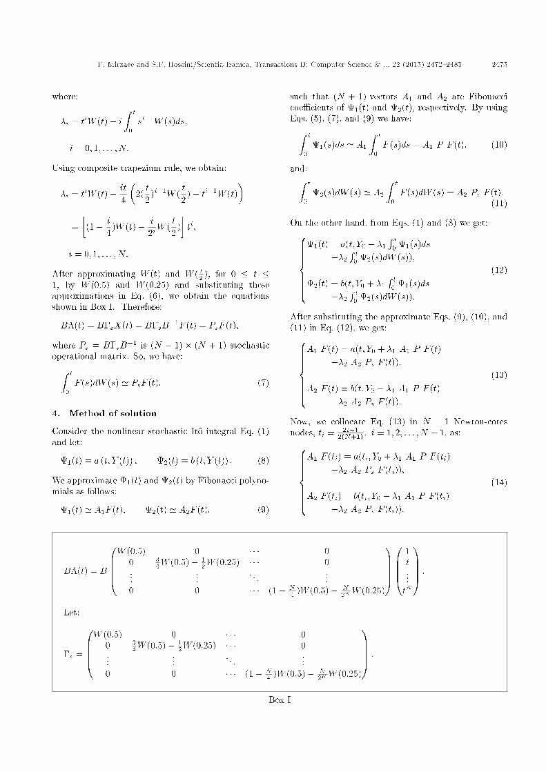
After approximating W (t) and W ( t2 ), for 0 � t �1, by W (0:5) and W (0:25) and substituting theseapproximations in Eq. (6), we obtain the equationsshown in Box I. Therefore:

B�(t) = B�sX(t) = B�sB�1F (t) = PsF (t);

where Ps = B�sB�1 is (N + 1) � (N + 1) stochasticoperational matrix. So, we have:Z t

0F (s)dW (s) ' PsF (t): (7)

4. Method of solution

Consider the nonlinear stochastic Ito integral Eq. (1)and let:

1(t) = a (t; Y (t)) ; 2(t) = b (t; Y (t)) : (8)

We approximate 1(t) and 2(t) by Fibonacci polyno-mials as follows:

1(t) ' A1F (t); 2(t) ' A2F (t); (9)

such that (N + 1)-vectors A1 and A2 are Fibonaccicoe�cients of 1(t) and 2(t), respectively. By usingEqs. (5), (7), and (9) we have:Z t

01(s)ds ' A1

Z t

0F (s)ds = A1 P F (t); (10)

and:Z t

02(s)dW (s) ' A2

Z t

0F (s)dW (s) = A2 Ps F (t):

(11)

On the other hand, from Eqs. (1) and (8) we get:8>>>>>><>>>>>>:1(t) = a(t; Y0 + �1

R t0 1(s)ds

+�2R t

0 2(s)dW (s));

2(t) = b(t; Y0 + �1R t

0 1(s)ds+�2

R t0 2(s)dW (s)):

(12)

After substituting the approximate Eqs. (9), (10), and(11) in Eq. (12), we get:8>>>>>><>>>>>>:

A1 F (t) = a(t; Y0 + �1 A1 P F (t)+�2 A2 Ps F (t));

A2 F (t) = b(t; Y0 + �1 A1 P F (t)+�2 A2 Ps F (t)):

(13)

Now, we collocate Eq. (13) in N + 1 Newton-cotesnodes, ti = 2i�1

2(N+1) ; i = 1; 2; : : : ; N + 1, as:8>>>>>><>>>>>>:A1 F (ti) = a(ti; Y0 + �1 A1 P F (ti)

+�2 A2 Ps F (ti));

A2 F (ti) = b(ti; Y0 + �1 A1 P F (ti)+�2 A2 Ps F (ti)):

(14)

B�(t) = B

0BBB@W (0:5) 0 � � � 0

0 34W (0:5)� 1

2W (0:25) � � � 0...

.... . .

...0 0 � � � (1� N

4 )W (0:5)� N2NW (0:25)

1CCCA0BBB@

1t...tN

1CCCA :

Let:

�s =

0BBB@W (0:5) 0 � � � 0

0 34W (0:5)� 1

2W (0:25) � � � 0...

.... . .

...0 0 � � � (1� N

4 )W (0:5)� N2NW (0:25)

1CCCA :

Box I


Finally, by solving this nonlinear system with Newton'smethod and determining A1 and A2, we obtain theapproximate solution of the problem as follows:

YN (t) = Y0 + �1 A1 P F (t) + �2 A2 Ps F (t):

5. Existence of the solution

Picard's iteration has been used to prove the existenceand uniqueness of the solution of stochastic integralequations. In [25], the authors used Schauder's �xedpoint theorem to give a new existence theorem aboutthe solution of a stochastic integral equation. The the-orem can weaken some conditions gotten by applyingBanach's �xed point theorem.

Theorem 2. Let Q = f(t; Y (t)) 2 R2; t 2 [0; T ];and jY (t)j � r for �xed r > 0g. Assume the followingconditions:

(i) a(t; Y (t)); b(t; Y (t)) : Q! R are continuous andmeasurable on [0; T ]� ;

(ii) We de�ne:

d = sup(t;Y (t))2Q

fjja(t; Y (t))jj; jjb(t; Y (t))jjg;

and let the real number T; d, and random variableh be given that:

3E[h2] + 3T (1 + T )d2 � r2:

(iii) We set M = fY (t) 2 X ; kY (t)k � rg in whichX denotes the space of all stochastic processesf(t; w); 0 � t � T that are adapted to �ltrate Ftand

R T0 E(jY (t)j2)dt < +1.

Then the stochastic integral Eq. (1) has at least onesolution Y (t) 2M .

Proof [25].

Theorem 3. Assume the following conditions:

(i) a(t; Y (t)) and b(t; Y (t)) are measurable on [0; T ]�;

(ii) ja(t; Y (t))� a(t;X(t))j � k1jY (t)�X(t)j, jb(t; Y(t))� b(t;X(t))j � k2jY (t)�X(t)j;

(iii) Let the real number T; c = maxfk1; k2g be givensuch that:

0 � 2Tc2(1 + T ) < 1:

Then the stochastic integral Eq. (1) has a uniquesolution Y (t) 2M .

Proof [25].

6. Convergence analysis

The Fibonacci polynomials can be expressed in termsof some orthogonal polynomials, such as Chebychevpolynomial of the second kind un(t) [26]. It can beshown that:

FN+1(t) = iNuN�t2i

�:

that i2 = �1; N � 0.As we know, the expansion of f(t) in the approx-

imated form of Fibonacci polynomials can be writtenas:

f(t) ' pn(t) =N+1Xi=1

aiFi(t):

On the other hand, it can eventually be expressed as:

pn(t) =NXj=0

cjuj(t);

where cj ; j = 0; 1; : : : ; N , can be expressed in termsof ai; i = 1; 2; : : : ; N + 1. If uj(t) =

q( 2� ) uj(t), then

uj(t); j = 0; 1; : : : ; N , form an orthonormal polynomialbasis in [�1; 1] with respect to weight function !(t) =(1 � t2) 1

2 , that can be mapped into [0; 1]. Therefore,this procedure yields:

pn(t) =NXj=0

r(

2�

) cjuj(t):

Golberg and Chen [27] proved that when we areapproximating a continuously di�erentiable function(g 2 Cr; r > 0) by Chebychev polynomials, then:

kg � pnk! < �N�r;

where � is some constant. So, above statements provethe following theorem.

Theorem 4. Suppose that Fn(g(t)) is expansion ofg(t) in Fibonacci basis. For all function g in C[0; 1],the sequence fFn(g); n = 1; 2; : : :g converges uniformlyto g.

Proof. Considering the above descriptions, proof isclear.

This theorem shows that for any g 2 C[0; 1] andfor any ", there exists n such that:

kFn(g)� gk < ":

We suppose k � k be the L2 norm on [0; 1]. We de�nethe error function as:

eN (t) = Y (t)� YN (t);


in which Y (t) and YN (t) are the exact and approximatesolution of Eq. (1), respectively. So, we have:

Y (t)� YN (t) = �1

Z t

0(1(s)� 1(s)) ds

+ �2

Z t

0(2(s)� 2(s)) dW (s);

where i(s); i = 1; 2, is de�ned in Eq. (8). Alsoi(s); i = 1; 2, is approximated form of i(s); i = 1; 2,by Fibonacci approximation.

Theorem 5. Let Y (t) be exact solution and YN (t)be the Fibonacci approximate solution of Eq. (1). Alsoassume that:

(i) For every T and K, there is a constant Ddepending only on T and K such that for alljZj; jY j � K and all 0 � t � T ,

ja(t; Z)�a(t; Y )j+jb(t; Z)�b(t; Y )j�DjZ�Y j:(ii) Coe�cients satisfy the linear growth condition:

ja(t; Z)j+ jb(t; Z)j � D(1 + jZj):(iii) E(jZj2) <1:

Then YN (t) converges to Y (t) in L2.

Proof.

eN (t) =�1

Z t

0(1(s)� 1(s))ds

+ �2

Z t

0(2(s)� 2(s))dW (s)

EkeN (t)k2 � 2�j�1j2Ek

Z t

0(1(s)� 1(s))dsk2

+j�2j2EkZ t

0(2(s)�2(s))dB(s)k2

�:

From Theorem 1, we have:

EkeN (t)k2 � 2�j�1j2

Z t

0Ek1(s)� 1(s)k2ds

+j�2j2Z t

0Ek2(s)� 2(s)k2ds

�� 8�j�1j2

Z t

0Ek1(s)�N

1 (s)k2ds

+j�1j2Z t

0EkN

1 (s)� 1(s)k2ds:

+j�2j2Z t

0Ek2(s)�N

2 (s)k2ds

+j�2j2Z t

0EkN

2 (s)� 2(s)k2ds�;

where N1 (s) = a(s; YN (s)) and N

2 (s) = b(s; YN (s)).By Theorem 4, there exists N > 0 such that for any ":

EkNj (s)� j(s)k2 � " =

"1

16j�j j2 ; j = 1; 2:

So:

EkeN (t)k2 � "1 + 8�j�1j2

Z t

0Ek1(s)�N

1 (s)k2ds

+j�2j2Z t

0Ek2(s)�N

2 (s)k2ds�:

Using Lipschitz condition:

EkeN (t)k2 � "1+8�j�1j2+j�2j2�D2

Z t

0EkeN (s)k2ds:

(15)

Hence from Eq. (15) and Gronwall inequality we have:

EkeN (t)k2 ! 0:

Therefore, YN (t)! Y (t) in L2.

7. Illustrative examples

To illustrate the e�ectiveness of the proposed method,three examples are carried out in this section. In thisregard, we have presented Tables 1 to 6. All resultsare computed by using a program written in Matlab.Using this method, all nonlinear examples reduce tononlinear systems of equations that we solve them byNewton's method with zero vector as the initial guess.

Let Y (t) be the exact solution and YN (t) be theFibonacci approximate solution of Eq. (1), then wede�ne the error in the interval [0; 1] as:

kEk1 = max jeN (ti)j; 0 � ti � 1;

where eN (ti) = Y (ti)� YN (ti).

Example 1 [8]. Consider the following nonlinearstochastic Ito-Voletrra integral equation:

Y (t) = 0:5 +Z t

0Y (s)(1� Y (s))ds

+0:25Z t

0Y (s)dW (s); 0 � t � 1; (16)

with the exact solution:

Y (t) =0:5exp(0:96875t+ 0:25W (t))

1 + 0:5R t

0 exp(0:96875t+ 0:25W (t))ds: (17)

This integral equation is a simple model for the size


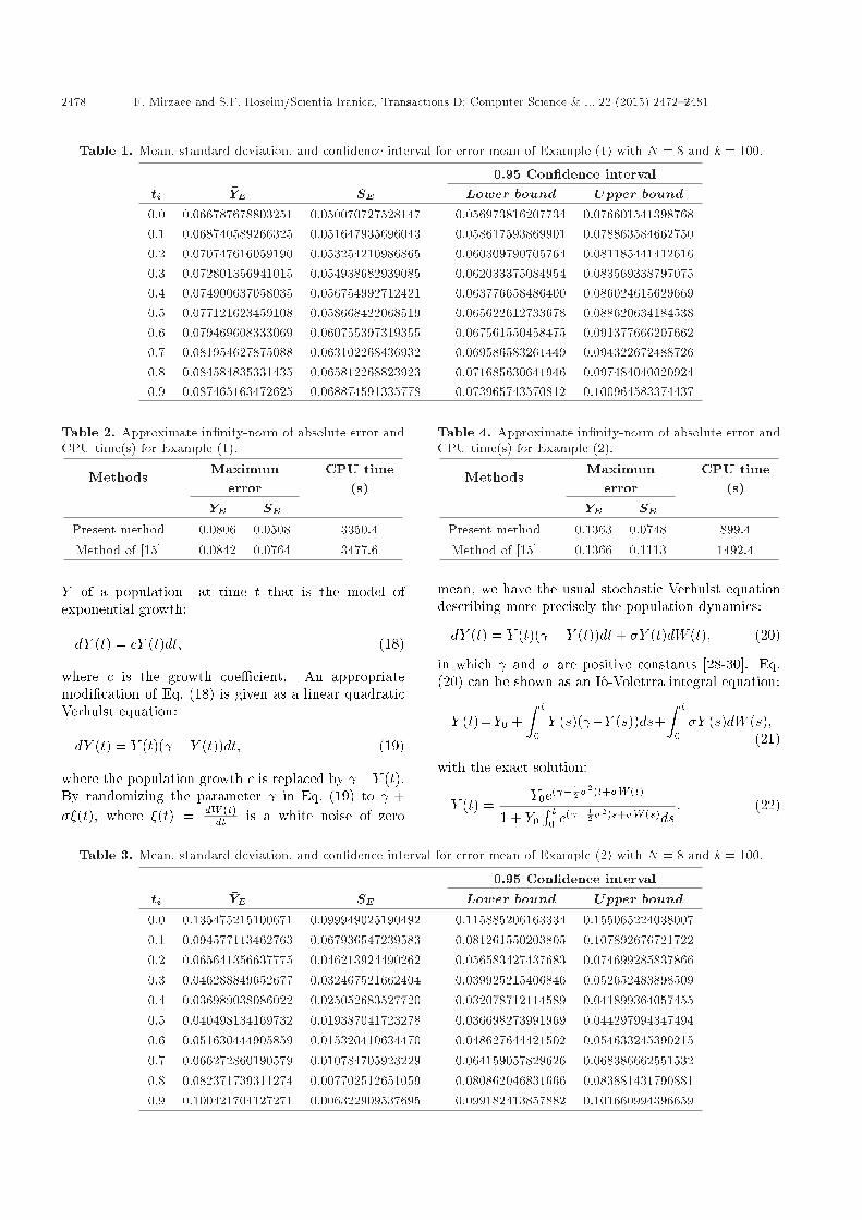
Table 1. Mean, standard deviation, and con�dence interval for error mean of Example (1) with N = 8 and k = 100.

0.95 Con�dence intervalti �YE SE Lower bound Upper bound0.0 0.066787678803251 0.050070727528147 0.056973816207734 0.0766015413987680.1 0.068740589266325 0.051647935696043 0.058617593869901 0.0788635846627500.2 0.070747616059190 0.053254210986865 0.060309790705764 0.0811854414126160.3 0.072801356941015 0.054938682939085 0.062033375084954 0.0835693387970750.4 0.074900637058035 0.056754992712421 0.063776658486400 0.0860246156296690.5 0.077121623459108 0.058668422068519 0.065622612733678 0.0886206341845380.6 0.079469608333069 0.060755397319355 0.067561550458475 0.0913776662076620.7 0.081954627875088 0.063102268436932 0.069586583261449 0.0943226724887260.8 0.084584835331435 0.065812268823923 0.071685630641946 0.0974840400209240.9 0.087465163472625 0.068874591335778 0.073965743570812 0.100964583374437

Table 2. Approximate in�nity-norm of absolute error andCPU time(s) for Example (1).

Methods Maximumerror

CPU time(s)

�YE SEPresent method 0.0806 0.0508 3350.4Method of [15] 0.0842 0.0764 3477.6

Y of a population at time t that is the model ofexponential growth:

dY (t) = cY (t)dt; (18)

where c is the growth coe�cient. An appropriatemodi�cation of Eq. (18) is given as a linear quadraticVerhulst equation:

dY (t) = Y (t)( � Y (t))dt; (19)

where the population growth c is replaced by �Y (t).By randomizing the parameter in Eq. (19) to +��(t), where �(t) = dW (t)

dt is a white noise of zero



CPU time(s)


mean, we have the usual stochastic Verhulst equationdescribing more precisely the population dynamics:

dY (t) = Y (t)( � Y (t))dt+ �Y (t)dW (t); (20)

in which and � are positive constants [28-30]. Eq.(20) can be shown as an Io-Voletrra integral equation:

Y (t)=Y0 +Z t

0Y (s)( �Y (s))ds+

Z t

0�Y (s)dW (s);

(21)


Y (t) =Y0e( � 1

2�2)t+�W (t)

1 + Y0R t

0 e( � 1

2�2)s+�W (s)ds: (22)


0.95 Con�dence intervalti �YE SE Lower bound Upper bound0.0 0.135475215100671 0.099949025190492 0.115885206163334 0.1550652240380070.1 0.094577113462763 0.067936547239583 0.081261550203805 0.1078926767217220.2 0.065641356637775 0.046213924490262 0.056583427437683 0.0746992858378660.3 0.046288849652677 0.032467521662404 0.039925215406846 0.0526524838985090.4 0.036989038086022 0.025052683527720 0.032078712114589 0.0418993640574550.5 0.040498134169732 0.019387041723278 0.036698273991969 0.0442979943474940.6 0.051630444905859 0.015320410634470 0.048627644421502 0.0546332453902150.7 0.066272860190579 0.010784705923229 0.064159057829626 0.0683866625515320.8 0.082371739311274 0.007702512651059 0.080862046831666 0.0838814317908810.9 0.100421704127271 0.006322909537695 0.099182413857882 0.101660994396659



0.95 Con�dence intervalti �YE SE Lower bound Upper bound

0.0 0.009355665647819 0.006755459612363 0.008031595563796 0.0106797357318420.1 0.031217002113644 0.024322569914853 0.026449778410333 0.0359842258169550.2 0.040897395484443 0.027392057364539 0.035528552240994 0.0462662387278930.3 0.048795606340377 0.038178679020026 0.041312585252452 0.0562786274283020.4 0.055188393237043 0.041477690239870 0.047058765950029 0.0633180205240580.5 0.061091301361998 0.045404732373637 0.052191973816765 0.0699906289072310.6 0.066550166176714 0.055272371925028 0.055716781279409 0.0773835510740200.7 0.074798297097570 0.057252918866680 0.063576724999701 0.0860198691954390.8 0.084017239030808 0.069273995253571 0.070439535961108 0.0975949421005080.9 0.097281470236254 0.074331818594678 0.082712433791697 0.111850506680811



CPU time(s)


By considering Y0 = 0:5; = 1; and � = 0:25in Eq. (21), we get Eq. (16) that can be solved bythe proposed method. The numerical results for thisexample are shown in Tables 1 and 2. In thesetables, �YE is the error mean and SE is the standarddeviation of errors in k iteration. In Table 2, wecompare the maximum absolute error and measuredCPU time(s) for the present method and Bernsteinfunctions method [15] with N = 8 and k = 20.


Y (t) = 1 +Z t

0Y (s)(

132� Y 2(s))ds

+0:25Z t

0Y (s)dW (s); 0 � t � 1; (23)


Y (t) =exp(0:25W (t))q

1 + 2R t

0 exp(0:5W (s))ds: (24)

The numerical results for this example are shown inTables 3 and 4. In these tables, �YE is the errormean and SE is the standard deviation of errors ink iteration. In Table 4, we compare the maximumabsolute error and measured CPU time(s) for thepresent method and Bernstein functions method [15]with N = 8 and k = 20.


Y (t) =18� 0:015625

Z t

0Y (s)(1� Y 2(s))ds

+0:125Z t

0(1� Y 2(s))dW (s); 0 � t � 1;

(25)


Y (t) =98e

0:25W (t) � 78

98e0:125W (t) + 7

8: (26)

The numerical results for this example are shown inTables 5 and 6. In these tables, �YE is the errormean and SE is the standard deviation of errors ink iteration. In Table 6, we compare the maximumabsolute error and measured CPU time(s) for thepresent method and Bernstein functions method [15],with N = 8 and k = 20.

8. Conclusion

Because it is almost impossible to �nd the exactsolution of Eq. (1), it would be convenient to determineits numerical solution based on stochastic numericalanalysis. This paper suggested a numerical methodto solve the nonlinear stochastic Ito-Volterra integralequations by using Fibonacci polynomials and theiroperational matrices. Moreover, the stochastic opera-tional matrix of Ito-integration for Fibonacci functionswas derived and the convergence and error analyses ofthe proposed method were established. E�ciency ofthis method and a good reasonable degree of accuracyis con�rmed by three numerical examples. Further-more, the results of the present method have beencompared with analytical solution and the solution ofBernstein method [15].


Acknowledgments

The authors are very grateful to referees and associateeditor for their comments and suggestions which haveimproved the paper.

References

1. Berger, M. and Mizel, V. \Volterra equations with Itointegrals", I. J. Int. Equ., 2, pp. 187-245 (1980).

2. Berger, M. and Mizel, V. \Volterra equations with Itointegrals", II. J. Int. Equ., 2, pp. 319-337 (1980).

3. Appley, J.A.D., Devin, S. and Reynolds, D.W. \Al-most sure convergence of solutions of linear stochasticVolterra equations to non-equilibrium limits", J. Integ.Equ. Appl., 19(4), pp. 405-437 (2007).

4. Pardoux, E. and Protter, P. \Stochastic Volterra equa-tions with anticipating coe�cients", Ann. Probab., 18,pp. 1635-1655 (1990).

5. Shiota, Y. \A linear stochastic integral equation con-taining the extended Ito integral", Math. Rep., 9, pp.43-65 (1986).

6. Khodabin, M., Maleknejad, K., Rostami, M. andNouri, M. \Numerical solution of stochastic di�erentialequations by second order Runge-Kutta methods",Math. Comput. Model., 53, pp. 1910-1920 (2011).

7. Khodabin, M., Maleknejad, K., Rostami, M. andNouri, M. \Interpolation solution in generalizedstochastic exponential population growth model",Appl. Math. Model., 36(3), pp. 1023-1033 (2012).

8. Kloeden, P.E. and Platen, E. \Numerical solutionof stochastic di�erential equations", Appl. Math.,Springer-Verlag, Berlin (1995).

9. Maleknejad, K., Khodabin, M. and Hosseini Shekarabi,F. \Modi�ed block pulse functions for numerical solu-tion of stochastic Volterra integral equations", J. Appl.Math., 2014, pp. 1-10 (2014).

10. Khodabin, M., Maleknejad, K. and Hosseini Shekarabi,F. \Application of triangular functions to numericalsolution of stochastic Volterra integral equations",IAENG Int. J. Appl. Math., 43(1), pp. 1-9 (2013).

11. Heydari, M.H., Hooshmandasl, M.R., Cattani, C.and Maalek Ghaini, F.M. \An e�cient computationalmethod for solving nonlinear stochastic Ito integralequations: Application for stochastic problems inphysics", J. Comput. Phys., 283, pp. 148-168 (2015).

12. Khodabin, M., Maleknejad, K. and Damercheli, T.\Approximate solution of the stochastic Volterra in-tegral equations via expansion method", Int. J. Indus.Math., 6(1), pp. 41-48 (2014).

13. Mirzaee, F. and Hadadiyan, E. \A collocation tech-nique for solving nonlinear stochastic Ito-Volterra inte-gral equations", Appl. Math. Comput., 247, pp. 1011-1020 (2014).

14. Mohammadi, F. \A wavelet-based computationalmethod for solving stochastic Ito-Volterra integralequations", J. Comput. Phys., 298, pp. 254-265(2015).

15. Asgari, M., Hashemizadeh, E., Khodabin, M. andMaleknejad, K. \Numerical solution of nonlinearstochastic integral equation by stochastic operationalmatrix based on Bernstein polynomials", Bull. Math.Soc. Sci. Math. Roumanie, 1, pp. 3-12 (2014).

16. Bhrawy, A.H. and Abdelkawy, M.A. \A fully spectralcollocation approximation formulti-dimensional frac-tional Schr�odinger equations", J. Comput. Phys., 294,pp. 462-483 (2015).

17. Bhrawy, A.H., Doha, E.H., Ezz-Eldien, S.S. andAbdelkawy, M.A. \A numerical technique based onthe shifted Legendre polynomials for solving the time-fractional coupled KdV equations", Calcolo (2015) (Inpress).

18. Bhrawy, A.H. and Zaky, M.A. \A method based onthe Jacobi tau approximation for solving multi-termtime-space fractional partial di�erential equations", J.Comput. Phys., 281, pp. 876-895 (2015).

19. Bhrawy, A.H. and Zaky, M.A. \Numerical simulationfor two-dimensional variable-order fractional nonlinearcable equation", Nonlinear Dyn., 80, pp. 101-116(2015).

20. Doha, E.H., Bhrawy, A.H. and Ezz-Eldien, S.S. \A newJacobi operational matrix: An application for solvingfractional di�erential equations", Appl. Math. Model.,36, pp. 4931-4943 (2012).

21. Klebaner, F., Introduction to Stochastic Calculus withApplications, Second Edition, Imperial college Press(2005).

22. Oksendal, B., Stochastic Di�erential Equations, an In-troduction with Applications, Fifth Edition, Springer-Verlag, New York (1998).

23. Falcon, S. and Plaza, A. \On k-Fibonacci sequencesand polynomials and their derivatives", Chaos SolitonFract., 39, pp. 1005-1019 (2009).

24. Mirzaee, F. and Hoseini, S.F. \Solving systems oflinear Fredholm integro-di�erential equations with Fi-bonacci polynomials", Ain Shams Engin. J., 5(1), pp.271-283 (2014).

25. Chen, X., Qi, Y. and Yang, C. \New existence the-orems about the solutions of some stochastic integralequations", arXiv preprint arXiv:1211.1249 (2012).

26. Rainville, E.D., Special Functions, New York (1960).

27. Golberg, M.A. and Chen, C.S., Discrete ProjectionMethods for Integral Equations, Southampton: Com-put. Mechanics Pub. (1997).

28. Gard, T.C., Introduction to Stochastic Di�erentialEquations, Marcel Dekker, New York (1988).

29. Gard, T.C. and Kannan, D. \On a stochastic di�eren-tial equations modeling of prey-predator evolution", J.Appl. Prob., 13, pp. 413-429 (1976).

30. Schoener, T.W. \Population growth regulated byintraspeci�c competition for energy or time: somesimple representations", Theor. Pop. Biol., 4, pp. 56-84 (1973).


Biographies

Farshid Mirzaee is Associate Professor at the Fac-ulty of Mathematical Sciences and Statistics, MalayerUniversity, Malayer, Iran. His research interests aremainly in the areas of numerical analysis, integral equa-tions, wavelets, orthogonal functions, fuzzy integralequations, stochastic analysis, and preconditioners.

Seyede Fatemeh Hoseini received her BS and MSdegrees in Applied Mathematics from Iran Universityof Science and Technology. She is currently PhDstudent of Malayer University in Applied Mathematicsat Malayer University under the supervision of Associ.Prof. Farshid Mirzaee. Her interests include numeri-cal analysis, ordinary di�erential equations, stochasticanalysis, wavelets, and integral equations.

Documents

Numerical approach for solving nonlinear stochastic It^o ...scientiairanica.sharif.edu/article_3797_390fb4db515fff7a60fccefe...Fibonacci functions and functions approximation by these