Embed Size (px)
Citation preview

Integration of System-Level Optimization with Concurrent Engineering Using Parametric Subsystem Modeling
by
Todd Schuman B.S. Engineering and Applied Science (Mechanical Engineering)
California Institute of Technology, 2002
Submitted to the Department of Aeronautics and Astronautics in partial fulfillment of the requirements for the degree of Master of Science in
Aeronautics and Astronautics at the
MASSACHUSETTS INSTITUTE OF TECHNOLOGY
June 2004
© 2004 Massachusetts Institute of Technology All rights reserved
Author ................................................................................................... Department of Aeronautics and Astronautics
May 24, 2003 Certified by ............................................................................................
Olivier L. de Weck Robert N. Noyce Assistant Professor of Aeronautics and Astronautics and
Engineering Systems Thesis Supervisor
Accepted by ...........................................................................................
Edward M. Greitzer H.N. Slater Professor of Aeronautics and Astronautics
Chair, Committee on Graduate Students

2

Integration of System-Level Optimization with Concurrent
Engineering Using Parametric Subsystem Modeling
by
Todd Schuman
Submitted to the Department of Aeronautics and Astronautics on May 24, 2004, in partial fulfillment of the
requirements for the degree of Master of Science in Aeronautics and Astronautics
Abstract
The introduction of concurrent design practices to the aerospace industry has greatly increased the efficiency and productivity of engineers during design sessions. Teams that are well-versed in such practices such as JPL’s Team X are able to thoroughly examine a trade space and develop a family of reliable point designs for a given mission in a matter of weeks compared to the months or years sometimes needed for traditional design. Simultaneously, advances in computing power have given rise to a host of potent numerical optimization methods capable of solving complex multidisciplinary optimization problems containing hundreds of variables, constraints, and governing equations. Unfortunately, such methods are tedious to set up and require significant amounts of time and processor power to execute, thus making them unsuitable for rapid concurrent engineering use. In some ways concurrent engineering and automated system-level optimization are often viewed as being mutually incompatible. It is therefore desirable to devise a system to allow concurrent engineering teams to take advantage of these powerful techniques without hindering the teams’ performance. This paper proposes such an integration by using parametric approximations of the subsystem models. These approximations are then linked to a system-level optimizer that is capable of reaching a solution more quickly than normally possible due to the reduced complexity of the approximations. The integration structure is described in detail and applied to a standard problem in aerospace engineering. Further, a comparison is made between this application and traditional concurrent engineering through an experimental trial with two groups each using a different method to solve the standard problem. Each method is evaluated in terms of optimizer accuracy, time to solution, and ease of use. The results suggest that system-level optimization, running as a background process during integrated concurrent engineering, is potentially advantageous as long as it is judiciously implemented from a mathematical and organizational perspective. Thesis Supervisor: Olivier L. de Weck Title: Assistant Professor of Aeronautics and Astronautics and of Engineering Systems
3

4

Acknowledgments
I would like to thank my advisor, Prof. Olivier L. de Weck, for providing me with ideas
and guidance whenever I needed them and for his continuous support during my graduate
career at MIT. I would also like to thank Dr. Jaroslaw Sobieszczanski-Sobieski, who graciously
supplied a wealth of knowledge on the BLISS method and helped create the motivational
backdrop for this project. Dr. Sobieski also provided the simplified model of the Space Shuttle
External Fuel Tank that was used as the case study for the life trials. I also acknowledge the
support of my former advisor at Caltech, Dr. Joel C. Sercel, who is one of the originators of the
ICEMaker software and method. Additional thanks to Dr. Hugh L. McManus for his advice on
projects from C-TOS to Space Tug. I am very grateful for the help and suggestions provided by
my fellow graduate students, with special recognition of those who participated in the live trial
exercise: Gergana Bounova, Babak Cohanim, Masha Ishutkina, Xiang Li, William Nadir, Simon
Nolet, Ryan Peoples, and Theresa Robinson. Finally, thanks to my friends for always standing
with me and to my family and Tory Sturgeon for their love and encouragement.
This research was supported by the MIT Department of Aeronautics and Astronautics
through a Teaching Assistant position. It was a great pleasure working with Prof. David Miller,
Prof. Jeffrey A. Hoffman, Col. John Keesee, Col. Peter W. Young, and all of the other Space
Systems Engineering staff and students.
5

6

Contents
1. Introduction.............................................................................15
1.1 Motivation................................................................................................................. 15
1.2 Integrated Concurrent Engineering............................................................................. 17
1.2.1 ICEMaker ............................................................................................................ 19
1.2.2 Improvements to ICEMaker.................................................................................. 22
1.3 Multidisciplinary Optimization ..................................................................................... 22
1.3.1 Genetic Algorithm Summary................................................................................. 23
1.3.2 Genetic Algorithm Procedure ................................................................................ 24
1.4 Problem Decomposition ............................................................................................. 26
1.5 Approximation Methods ............................................................................................. 29
1.6 Extensions of BLISS................................................................................................... 33
2. The ISLOCE Method .................................................................35
2.1 Implementation Overview .......................................................................................... 35
2.2 Implementation Specifics ........................................................................................... 37
2.2.1 Changes to ICEMaker .......................................................................................... 37
2.2.2 Software Specifics ............................................................................................... 38
2.2.3 Coding Issues...................................................................................................... 46
3. ISLOCE Method Live Trial.........................................................48
3.1 Trial Motivation ......................................................................................................... 48
3.2 Experimental Problem Description .............................................................................. 49
3.2.1 Model Introduction .............................................................................................. 49
3.2.2 Problem Setup..................................................................................................... 51
3.3 Trial Overview........................................................................................................... 58
3.3.1 Specific Trial Objectives ....................................................................................... 59
7

3.3.2 Trial Procedure.................................................................................................... 60
3.4 Evaluation Metrics ..................................................................................................... 64
3.5 Live Test Results ....................................................................................................... 67
3.5.1 Control Group Results Summary ........................................................................... 67
3.5.2 Control Group Performance .................................................................................. 70
3.5.3 Optimization Group Results Summary ................................................................... 71
3.5.4 Optimization Group Performance .......................................................................... 74
3.5.5 Combined Results and Comparisons ..................................................................... 76
4. Summary and Conclusions.......................................................83
4.1 Conclusions............................................................................................................... 83
4.2 Recommendations for Future Work............................................................................. 83
4.2.1 Refinement of Optimization Chair and Sheet Implementation ................................. 83
4.2.2 Comparison of CO, BLISS, and ISLOCE ................................................................. 84
4.2.3 Application of ISLOCE to an Industrial Strength Problem........................................ 85
4.2.4 Background Optimization Improvements ............................................................... 85
4.2.5 Refinement of EFT Pareto Front ........................................................................... 85
4.2.6 Trial Repetition.................................................................................................... 86
A. Appendix ..................................................................................87
A1 – Space Tug Concurrent Engineering Example ............................................................. 87
A1.1 Space Tug Introduction ........................................................................................ 88
A1.2 The MATE Method ................................................................................................ 89
A1.3 ICE Method.........................................................................................................102
A1.4 Case Study Observations .....................................................................................109
A2 – Catalog of ICEMaker and ISLOCE code ....................................................................112
A2.1 – Root Directory ..................................................................................................112
A2.2 – Client Subsystems ............................................................................................113
A2.3 – Project Server ..................................................................................................113
A2.4 – Saved Session Information................................................................................114
A2.5 – Optimization Chair ............................................................................................114
A3 – ISLOCE Tutorial......................................................................................................116
8

A3.1 ICEMaker Session Initialization .............................................................................116
A3.2 Client Operation ..................................................................................................116
A3.3 Optimization Chair Operation (optional) ................................................................117
A4 – Additional Figures and Tables..................................................................................118
Bibliography................................................................................120
9

List of Figures
Figure 1 – ICEMaker setup.................................................................................................. 20
Figure 2 – Genetic algorithm flowchart ................................................................................ 26
Figure 3 – BLISS system structure....................................................................................... 28
Figure 4 – Neural network iteration loop.............................................................................. 31
Figure 5 – Simple Neuron Model ........................................................................................ 31
Figure 6 – Example transfer function .................................................................................. 32
Figure 7 – Full neural network model ................................................................................. 33
Figure 8 - Foreground and background processes ................................................................ 36
Figure 9 - Simplified test case block diagram ....................................................................... 40
Figure 10 – Structures model neural network training data ................................................... 42
Figure 11 – Structures model neural network performance predicting total tank mass (R~1) .. 42
Figure 12 – Structures model neural network performance predicting cone stress (R~0.91) ... 43
Figure 13 – Viable EFT individuals discovered by genetic algorithm ....................................... 45
Figure 14 – (Pareto) Non-dominated individuals ................................................................... 45
Figure 15 – Space shuttle external fuel tank ........................................................................ 50
Figure 16 – EFT model components .................................................................................... 51
Figure 17 – EFT model stresses........................................................................................... 53
Figure 18 – Control group trade space exploration ............................................................... 69
Figure 19 – Optimization group trade space exploration ....................................................... 73
Figure 20 – Combined trade space exploration (circle: control, square: optimization) ............. 77
Figure 21 – Normalized Pareto front generated by extended GA run offline and used as “true”
Pareto front (circle: control, square: optimization, diamond: Pareto) ............................... 78
Figure 22 – Nominal single attribute utility for ∆V................................................................. 91
10

Figure 23 – ∆V utility for GEO-centric user ........................................................................... 92
Figure 24 – ∆V for ∆V hungry user ...................................................................................... 92
Figure 25 – Trade space for nominal user, with propulsion system indicated.......................... 98
Figure 26 – Trade space for nominal user, with capability indicated....................................... 98
Figure 27 – Trade space for capability stressed user............................................................. 99
Figure 28 – Trade space for response time stressed user...................................................... 99
Figure 29 – Trade space for user with large delta-V needs...................................................100
Figure 30 – Low capability systems, showing effect of increasing fuel load, with GEO rescue
vehicles ......................................................................................................................100
Figure 31 – ICE model components and interactions ...........................................................104
Figure 32 – Cryo one-way tug, showing extremely large fuel tanks; Bi-prop tug appears similar
..................................................................................................................................106
Figure 33 – Electric Cruiser (GEO round-trip tug) ................................................................106
Figure 34 – Comparison of all GEO tug designs ...................................................................107
Figure 35 – Mass breakdown of Electric Cruiser design ........................................................107
Figure 36 – Promising designs............................................................................................111
Figure 37 – Aerodynamics model neural network training data.............................................118
Figure 38 – Aerodynamics model neural network performance predicting payload (R~1).......118
Figure 39 – Cost model neural network training data...........................................................119
Figure 40 – Cost model neural network performance predicting total cost (R~1)...................119
11
List of Tables Table 1 – Live trial participants ........................................................................................... 67
Table 2 – Control group point designs ................................................................................. 70
Table 3 – Control group performance summary.................................................................... 71
Table 4 – Optimization group point designs ......................................................................... 74
Table 5 – Optimization group performance summary............................................................ 76
Table 6 – Combined live trial performance metrics ............................................................... 80
Table 7 – Manipulator capability attribute, with corresponding utility and mass ...................... 94
Table 8 – Utility weightings................................................................................................. 94
Table 9 – Propulsion system choices and characteristics ....................................................... 94
Table 10 – Miscellaneous coefficients .................................................................................. 96
Table 11 – GEO Tug Design Summary ................................................................................105
12
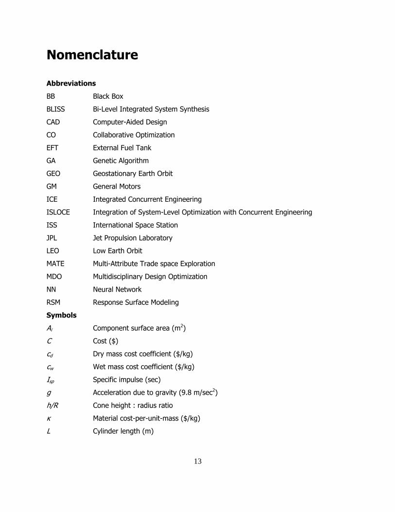
Nomenclature
Abbreviations
BB Black Box
BLISS Bi-Level Integrated System Synthesis
CAD Computer-Aided Design
CO Collaborative Optimization
EFT External Fuel Tank
GA Genetic Algorithm
GEO Geostationary Earth Orbit
GM General Motors
ICE Integrated Concurrent Engineering
ISLOCE Integration of System-Level Optimization with Concurrent Engineering
ISS International Space Station
JPL Jet Propulsion Laboratory
LEO Low Earth Orbit
MATE Multi-Attribute Trade space Exploration
MDO Multidisciplinary Design Optimization
NN Neural Network
RSM Response Surface Modeling
Symbols
Ai Component surface area (m2)
C Cost ($)
cd Dry mass cost coefficient ($/kg)
cw Wet mass cost coefficient ($/kg)
Isp Specific impulse (sec)
g Acceleration due to gravity (9.8 m/sec2)
h/R Cone height : radius ratio
κ Material cost-per-unit-mass ($/kg)
L Cylinder length (m)
13

l Seam length (m)
λ Seam cost-per-unit-length ($/m)
Mb Bus mass (kg)
mbf Bus mass fraction coefficient
Mc Mass of observation/manipulator system (kg)
Md Dry mass (kg)
Mf Fuel mass (kg)
mi Component mass (kg)
Mp Mass of propulsion system (kg)
mp Payload mass (kg)
mp0 Propulsion system base mass (kg)
mpf Propulsion system mass fraction coefficient
Mw Wet mass (kg)
Mt Total tank mass (kg)
pn Nominal tank payload (kg)
ρ Material density (kg/m3)
R Tank radius (m)
σ Component stress
t1 Cylinder thickness (m)
t2 Sphere thickness (m)
t3 Cone thickness (m)
Utot Total utility
Vc Single attribute utility for capability
Vt Single attribute utility for response time
Vv Single attribute utility for delta-V
Wc Utility weighting for capability
Wt Utility weighting for response time
Wv Utility weighting for delta-V
x Input design vector
∆v Change in velocity (m/sec)
ζ Vibration factor
14

1. Introduction 1.1 Motivation
The motivation for this project lies at the intersection of three ongoing areas of
research: integrated concurrent engineering, multidisciplinary optimization, and problem
decomposition. All three are relatively new fields that have quickly gained acceptance in the
aerospace industry. Integrated concurrent engineering (ICE) is a collection of practices that
attempts to eliminate inefficiencies in conceptual design and streamline communication and
information sharing among a design team. Based heavily on methods pioneered by the Jet
Propulsion Laboratory’s Team X, concurrent engineering practices have been adopted by major
engineering company sectors like Boeing’s Integrated Product Teams and General Motors’
Advanced Technology Design Studio. Multidisciplinary optimization is a formal methodology for
finding optimum system-level solutions to engineering problems involving many interrelated
fields. This area of research has benefited greatly from advances in computing power, and has
made possible a proliferation of powerful numerical techniques for attacking engineering
problems. Multidisciplinary optimization is ideal for most aerospace design, which traditionally
requires a large number of interfaces between complex subsystems. Problem decomposition is
a reaction to the ever-increasing complexity of engineering design. Breaking a problem down
into more manageable sub-problems allows engineers to focus on their specific fields of study.
It also increases efficiency by encouraging teams to work on a problem in parallel.
Modern engineering teams that are well versed in these practices see a significant
increase in productivity and efficiency. However, the three areas do not always work in
harmony with one another. One of the biggest issues arises from tension between
multidisciplinary optimization and problem decomposition. Decomposing a problem into smaller
pieces makes the overall problem more tractable, but it also makes it more difficult for system-
15

level optimization to make a meaningful contribution. Linking together a number of separate
(and often geographically distributed) models is not an easy coding task. As the complexity of
the various subsystems grows, so too does the size of the model needed to perform the
system-level optimization. It is possible to optimize all of the component parts separately at the
subsystem level, but this does not guarantee an optimal design. Engineering teams often
resign themselves to coding the large amount of software needed to address this problem. For
aerospace designs, an optimization run can take many days or even weeks to finish. This
introduces a factor of lag time into the interaction between the optimization staff and the rest of
the design team distances the two groups from each other. While waiting for the optimization
results to come back, the design team presses on with their work, often updating models and
reacting to changes in the requirements. When an optimization does finally produce data, the
results are often antiquated by these changes. This is of particular concern for concurrent
engineering, which strives to conduct rapid design. ICE teams cannot afford to wait for weeks
on end for optimization data when performing a trade analysis. On a more practical level, an
integrated engineering team and a computer-based optimizer cannot be allowed to operate on
the same design vector for fear of overriding each other’s actions. Thus, there is a fundamental
conflict between these three fields that must be carefully balanced throughout the design cycle.
This paper introduces a new method that addresses this conflict directly. It is an
attempt to unify multidisciplinary optimization with problem decomposition in an integrated
concurrent engineering environment. Known as ISLOCE (for ‘Integrated System-Level
Optimization for Concurrent Engineering’), this method has the potential to put the power of
modern system-level optimization techniques in the hands of engineers working on distributed
problems while retaining the speed and efficiency of concurrent engineering practices.
To evaluate this method, an aerospace test case is used. A simplified model of the
Space Shuttle external fuel tank (EFT) is adopted for use with ISLOCE. An experimental setup
is used to evaluate the benefits and issues of the method through a comparison to a more
conventional concurrent engineering practice. This setup allows for validation of the approach
in a full design environment. Before describing the details of the method, it is necessary to
introduce more fully the concepts upon which ISLOCE is based.
16

1.2 Integrated Concurrent Engineering
The traditional engineering method for approaching complicated aerospace design has
been to attack the problem in a linear fashion. Engineers are assembled into teams based on
their areas of expertise and the subsystems of the vehicle being designed. For example, a
typical aircraft design could be broken down into disciplines such as aerodynamics, propulsion,
structures, controls, and so on. A dominant subsystem is identified as one that is responsible
for satisfying the most critical requirements. The corresponding subsystem team begins its
work and develops a design that meets these requirements. This design is passed on to the
next most dominant subsystem and so on. The decisions made by each team thus become
constraints on all subsequent teams. In the aircraft example, the aerodynamics team could
determine a wing shape and loading that meets performance requirements on takeoff and
landing speeds, lift and drag coefficients, etc. This wing design is passed on to structures
group who, in addition to meeting whatever specific requirements they have on parameters like
payload capacity, vibration modes, and fuel capacity, must now accommodate securing this
wing design to the aircraft body. The propulsion team has to fit their power plant in whatever
space remains in such a way as to not violate any previous requirements, and finally the
controls team must develop avionics and mechanical controls to make the aircraft stable.
This example is obviously a simplification, but it illustrates a number of disadvantages of
a linear design process. Foremost among these is the inability to conduct interdisciplinary
trades between teams. With a linear design process, upstream decisions irrevocably fix
parameters for all downstream teams. There is little or no opportunity to go back and revise
previous parts of the design in order to achieve gains in performance or robustness or
reductions in cost. A certain wing design could require a large amount of structural
reinforcement resulting in increased mass, a larger power plant, and decreased fuel efficiency.
It should be possible to examine this result and then modify the wing design in such a way that
reduces the mass of the structural reinforcement at the cost of a small penalty in wing
performance. The gains achieved by this change could far outweigh the decrease in
performance and therefore would be a good decision for the overall project. These cascade
17

effects are a result of the interconnectedness of aerospace subsystems and are ubiquitous in
complex design problems.
Traditional design inhibits these interdisciplinary trades, not because they are
undesirable, but because of a lack of communication among subsystem teams. Engineering
teams typically focus their efforts on their particular problems and do not receive information
about what other teams are working on. Even when a group considers design changes that will
directly affect other teams, they are not notified of possible changes in a timely manner,
resulting in wasted efforts and inefficient time usage. Information is scattered throughout the
project team, meaning those seeking data on a particular subject have no central location to
search. Engineers thus spend a significant fraction of time not developing new information, but
rather searching for information that already exists.
Integrated concurrent engineering (ICE) has emerged as a solution to the major
problems associated with aerospace design, including complicated interdisciplinary interfaces
and inefficient time usage. Fundamentally, ICE addresses these issues by:
• Encouraging communication between subsystem teams
• Centralizing information storage
• Providing a universal interface for parameter trading
• Stimulating multidisciplinary trades
Rather than focusing on individual team goals, engineers meet frequently to discuss issues
facing the project as a whole. All pertinent project information is centralized so that anyone
can obtain information from every team with minimal effort.
ICE offers many advantages over conventional design methods. It acts to streamline
the entire design process, reducing inefficiencies caused by communication bottlenecks and
eliminating wasted work on outdated designs. Once an ICE framework is established, inter-
and intra-subsystem trades are clearly defined. This allows teams to work independently on
problems local to a subsystem and to coordinate effectively on issues that affect other teams.
ICE also provides for near-instantaneous propagation of new requirements. Projects using ICE
are more flexible and can quickly adapt to changes in top-level requirements. All these factors
18
together allow engineering teams to conduct rapid trades among complex multidisciplinary
subsystems. Teams that are well-versed in such practices are able to thoroughly examine a
trade space and develop a family of reliable point designs for a given mission in a matter of
weeks compared to the months or years sometimes needed for traditional design.
1.2.1 ICEMaker
Parameter-trading software has become an integral part of ICE teams, allowing users to
quickly share information and update each other of changes to the design. This software
serves not only as a central server for information storage but also as a tool for establishing a
consistent naming convention for information so that all engineers know that they are referring
to the same information. Caltech’s Laboratory for Spacecraft and Mission Design has made
several important contributions to the ICE method, including software known as ICEMaker that
was used throughout this project.1
ICEMaker is a parameter exchange tool that runs in Excel and facilitates sharing of
information amongst the design team. ICEMaker has a single-server / multiple-client interface.
With ICEMaker, a design problem is broken down into modules or subsystems with each
module (‘client’) consisting of a series of computer models developed by the corresponding
subsystem team. These models are developed offline, a process that can take anywhere from a
few days to a few months depending on the desired level of model fidelity. During a design
session, each client is interactively controlled by a single team representative (‘chair’). The
individual clients are linked together via the ICEMaker server. Chairs can query the server to
either send their latest numbers or receive any recent changes made in other clients that affect
their work. The querying process is manual, preventing values from being overwritten without
permission from the user. Design sessions using ICEMaker typically last three hours and usually
address one major trade per design session. A senior team member (‘facilitator’) leads the
design sessions and helps to resolve disconnects between the clients. Design sessions are
iterative, with each subsystem sending and receiving many times in order for the point design
to converge. Although it has recently become possible to automate this iterative process,
19

human operation of the client stations is almost always preferred. The human element and the
ability to catch bugs or nonsensical parameters are crucial to the ICE process. The necessity of
keeping humans in the loop will be discussed in greater detail in a later section.
Figure 1 – ICEMaker setup
As shown in figure 1, the ICEMaker server maintains the complete list of all parameters
available to the design team. Before beginning a project, an ICEMaker server creates all of the
clients that will be used during the design sessions. Additional clients can be added later if
needed. During a design session, the server notes all ‘send’ and ‘receive’ requests made by the
clients. This information is time-stamped so that the facilitator can track the progress of an
iteration loop and know how recent a set of data is. Any errors that are generated by the code
are also displayed in the server, with the most common being multiple subsystems attempting
to publish the same information and a single subsystem publishing duplicate parameters. In
general, the server runs on an independent computer and is checked occasionally by the
facilitator but otherwise stays in the background for most of a design session. The server is
20

never run on the same machine as a client as this generates conflicts between the code and
leads to session crashes.
The basic ICEMaker client initializes in Excel with three primary worksheets. The input
sheet tracks all parameters coming into a client and all associated data including parameter
name, value, units, comments, what client provides the parameter, and when the parameter
was last updated. A single macro button downloads all of the most current information from
the server to the client. The output sheet lists all parameters that a client sends to other
clients, with most of the same information as the input sheet. Again, a one-click macro sends
all current data to the ICEMaker server. Finally, a project status sheet gives a summary of all
available and requested parameters. A client operator can use this sheet to claim parameters
requested by other subsystems or to add additional input parameters to the input sheet. In
addition to these three main sheets, a finished ICEMaker client will also have several user-
designed sheets. These sheets contain all of the calculations need to process the input data
and calculate the output data.
It is important to note that ICEMaker is not an all-in-one automated spacecraft or
aircraft generator, nor is it a high-end symbolic calculation tool. It simply serves as a
compliment to the ICE method by enabling multidisciplinary trades through parameter sharing.
The end designs developed using ICEMaker are only as accurate as the models they are based
on. With this in mind, there are many problems that are unsuitable for ICEMaker usage.
Typically, models for ICEMaker clients are developed with Excel or with software that is easily
linked to Excel such as Matlab. CAD or finite-element programs are more difficult to interface.
Furthermore, the data that can be transferred through ICEMaker is limited to those formats
capable of being expressed in an Excel cell, typically real numbers or text strings. Approximate
geometry, timelines, and other qualitative information are very difficult to express in this way.
ICEMaker is most powerful for tackling highly quantitative problems with well-defined interfaces
between subsystems. Recognizing both the potential and the limitations of ICEMaker is
essential for proper usage.
21

1.2.2 Improvements to ICEMaker
While a powerful tool in its own right, attempts have been made to improve upon
ICEMaker by incorporating automated convergence and optimization routines into the program.
Automatic convergence presents no major problems as the routine simply mimics the role of a
human operator by querying each of the clients in turn and updating the server values
published by each client. Optimization algorithms have proven more difficult to implement.
Each module is usually designed with subsystem-level optimization routines built in that are
capable of producing optimal values for the inputs provided to it based on whatever metrics are
desired. However, even if every subsystem is optimized in this way, there is no guarantee that
the design is optimized at the system level. A system-level optimizer for ICEMaker that queried
each module directly when producing a design vector would require a tremendous amount of
time and computing resources to run, especially for problems with thousands of variables with
complicated non-linear relations between them. At the same time, the human team would be
unable to work on a design while the optimizer was running as any values they changed would
likely be overwritten by the optimizer as it searched for optimal solutions. Such an optimizer
would not be conducive to rapid design and is therefore unsuitable for this problem. It is
therefore desirable to develop an optimization method that complements the concurrent
engineering practices currently in use.
1.3 Multidisciplinary Optimization
For most traditional aerospace systems, optimization efforts have focused primarily on
achieving desired levels of performance through the variation of a small number of critical
parameters.2 In the aircraft design described in the introduction, wing loading and aspect ratio
serve as good examples of obvious high-level parameters that have far-reaching consequence
on the rest of the vehicle. The approach has worked fairly well in the past because these
critical parameters are in fact the dominant variables for determining aircraft performance.
Recently however, other subsystems such as structures and avionics have started to play a
more prominent role in aerospace design. The highly-coupled interactions of these subsystems
have driven up the number of design parameters which have a major impact on the
22

performance of an aerospace design. Further, even after optimization has been performed
through critical parameter variation, there is still a certain amount of variability in the residual
independent parameters whose values have a non-trivial effect on a vehicle’s performance.
Even a small improvement in the performance or cost can mean the difference between a viable
program and a complete failure. The ability to perform a system-level optimization with many
critical parameters displaying complex interactions is of the highest importance in modern
engineering design. Consequently, a number of new numerical techniques have been
developed to enable engineers to meet this challenge and produce designs that are as close as
possible to being mathematically optimal.
1.3.1 Genetic Algorithm Summary
A genetic algorithm is an optimization method based on the biological process of natural
selection. Rather than using a single point design, a genetic algorithm repeatedly operates on a
population of designs. Each individual of the population represents a different input vector of
design variables. Every individual’s performance is evaluated by a fitness function, and the
most viable designs are used as ‘parents’ to produce ‘offspring’ designs for the next generation.
Over time, the successive generations evolve towards an optimal solution.
Genetic algorithms have a number of features that make them attractive for
multidisciplinary optimization. GAs are well suited for solving problems with highly non-linear
discontinuous trade spaces like those commonly found in aerospace design. Especially in early
conceptual design, aerospace designers are often interested not in finding just one particular
solution to a problem but a family of solutions that span a wide range of performance criteria.
This set of solutions can then be presented to the customer or sponsor who can choose from
among them the design that best meets his or her metrics of performance. Genetic algorithms
can meet this need by solving for a front of Pareto-dominant solutions (those for which no
increase in the value of one objective can be found without decreasing the value of another).
Furthermore, this method helps elucidate not only the performance trades but also the
sensitivity of these trades and their dependence upon the input parameters. In this way,
23

genetic algorithms help provide a much fuller understanding of the trade space than do
gradient-based techniques.
1.3.2 Genetic Algorithm Procedure
This section describes the basic operation of a genetic algorithm. It should provide a
level of knowledge adequate for understanding the role of the GA in this report. Due to the
diversity of different types of genetic algorithms, this will not be an exhaustive coverage of the
topic. Discussion will focus almost entirely on the specific GA used in a later section. Additional
sources of information can be found in the references section if desired.3
To begin, a genetic algorithm requires several pieces of information. First, the
parameter space must be defined with lower and upper bounds for each input variable. A
starting population is often provided if the parameter space is highly constrained or has very
small regions of viable solutions. Many GAs, including the one used for this project, encode
each individual as a string of bits. Bit encoding allows for a uniform set of basic operators to be
used when evaluating the GA, simplifying the analysis but possibly resulting in performance
decreases. If bit encoding is used, the number of bits allocated to each variable in the design
vector is also specified. More bits are required for representing real numbers than simple
integers, for example.
Next, a fitness function is developed that represents the metric used to evaluate the
viability of an individual and determine whether its characteristics should be carried on to the
next generation. For many optimization problems, the fitness function is simply the function
whose optimum value is sought. However, as discussed previously, for many aerospace
optimization problems it is not a single optimum value but a family of Pareto-optimal solutions
that is desired. The EFT model uses this latter approach. To accomplish this, each individual of
a population is first evaluated according to the conventional method in order to determine its
performance. The fitness function then compares the output vector of an individual to every
other output vector in the population. A penalty is subtracted from the fitness of the individual
for each other member found whose output vector dominates that of the individual being
24

evaluated. Additional fitness penalties are imposed on individuals that violate any of the
problem constraints, with the severity of the penalty proportional to the severity of the
violation. In this way, the fittest individuals are those that dominate the most number of other
solutions while at the same time conforming to all of the constraints as closely as possible,
although some amount of fitness function parameter tweaking is required to observe this
behavior in practice.
Finally, it is necessary to set values for a number of options that dictate how the genetic
algorithm will progress once it is started. The number of individuals per generation and the
number of generations must both be specified. Larger populations increase the number of
points evaluated per generation and create a wider spread of points, but can bog down the GA
if the time required to evaluate each individual is long. Increasing the number of generations
gives the GA more time to evolve towards the Pareto front, but similarly increases the amount
of time required for the algorithm to run. Also, two probabilities must be defined. The first is
the crossover probability. During the reproduction phase between generations, the crossover
probability is the chance that a pair of parent individuals will be combined to produce a new
offspring individual. A high probability means that most high-fitness members will be combined
to form children, while a low probability means that most high-fitness individuals will pass
unaltered into the next generation. This number is usually set high (> 0.9), although certain
problems require a lower value. The second probability is the mutation probability. After the
reproduction phase, the values of some individuals’ input vectors are randomly altered based on
this probability. Mutation helps ensure that a population’s evolution does not stagnate in a local
optimum and allows the population to discover viable areas of the trade space. A low mutation
probability leads to somewhat faster convergence but has an adverse effect on how close the
population comes to approaching the true optimum. High mutation means that it is more
difficult for a large number of strong individuals to emerge from the reproduction phase
unaltered. Figure 2 shows the typical flow of a genetic algorithm.
25

Figure 2 – Genetic algorithm flowchart4
1.4 Problem Decomposition
As engineering problems grow in complexity, so too grow the models necessary to solve
these problems. This increased complexity translates directly to a greater number of required
calculations, longer model evaluation times, and slower design development. One way of
overcoming this obstacle is through problem decomposition. Problem decomposition breaks a
down large design problems into more tractable sub-problems. It takes advantage of the
diversity in design experience each designer brings to the table and allows advances in one
discipline to be incorporated into the work of every other. In addition to the benefits gained
from focusing engineers on specific disciplines (rather than broad areas), this division
encourages engineering teams to work in parallel and reduce end-to-end model run-time.
Recently, multidisciplinary optimization has been combined with problem decomposition
to help provide an overarching framework for the design. A careful balance must be struck
between giving the disciplines autonomy over their associated subsystems and ensuring that
26

decisions are made that benefit the project at a system level and not just the performance of an
individual subsystem. A number of techniques have emerged in an attempt to integrate these
two areas of research.
One such approach, known as collaborative optimization (CO), has been developed by
Braun and Kroo at Stanford University.5 , 6 This approach divides a problem along disciplinary
lines into sub-problems that are optimized according to system-level metrics of performance
through a multidisciplinary coordination process. Each sub-problem is optimized so that the
difference between the design variables and the target variables established by the system
analyzer is at a minimum. This combination of system optimization with system analysis is
potent, but leads to setups with high dimensionality. This result can drastically increase the
amount of processing power needed to run even a simple optimization. CO (like most other
distributed methods) is most effective for problems with well-defined disciplinary boundaries, a
large number of intra-subsystem parameters and calculations, and a minimum of
interdisciplinary coupling. CO has been successfully applied to a number of different
engineering problems ranging from vehicle design to bridge construction.7
Another leading method is bi-level integrated system synthesis (BLISS), developed by J.
Sobieski, Agte, and Sandusky at the NASA Langley Research Center.8 Like CO, BLISS is a
process used to optimize distributed engineering systems developed by specialty groups who
work concurrently to solve a design problem. The main difference with CO is that the quantities
handed down from the system level in BLISS are not targets, but preference weights that are
used for multi-objective optimization at the subsystem level. Constraints and coupling variables
are also handled somewhat differently. The system objectives are used as the optimization
objectives within each of the subsystems and at the system level. These two levels of
optimization are coupled by the optimum sensitivity derivatives with respect to the design
parameters. The design parameters are divided into three groupings. So-called X-variables are
optimized at the local level and are found only within each of the subsystems. Y-variables are
those which are output by one subsystem for use in another. Finally, system-level design
variables are denoted as Z-variables, with system-level denoting variables shared by at least
two subsystems. This setup is illustrated in figure 3.
27

Figure 3 – BLISS system structure9
A BLISS session begins with optimization at the subsystem level. The system-level variables are
treated as constants and each subsystem attempts to improve on the objective function. Then,
the system computes the derivatives of the optimum with respect to the frozen parameters.
The next step is an attempt at improving the objective function by modifying the system-level
variables. This step is linked to the first step via the optimum sensitivity derivatives. In this
way, the sub-domain X values are expressed as functions of the Y and Z variables. The two
steps alternate until the desired level of convergence is reached.
This setup has a number of advantages. The system structure is modular, which allows
black boxes to be added, modified, or replaced. This allows engineers to perform calculations
with different levels of fidelity at different stages of design. In this way, it is possible to use
coarse, high-speed models early on in design when rapid trade space exploration is desired
then switch over to higher fidelity models later when more accurate assessments are required.
Another benefit is the ability to interrupt the optimization process in between cycles, allowing
human intervention and the application of judgment and intuition to the design. Future
28

research will attempt to compare the performance and ease of use of these methods for a set
of benchmark cases. Both rapid design capability and insistence upon human incorporation into
design processes stand out as highly desirable features to have in a modern design method.
BLISS’s separation of overall system design considerations from subsystem-level detail also
makes it a good fit for diverse, dispersed human teams and is a model to be emulated in
ISLOCE.
1.5 Approximation Methods
As discussed in the previous section the pattern of work distribution via problem
decomposition has become commonplace in many industrial settings. However, this approach
does not make the job of a system-level optimizer any easier. To run a high-fidelity system-
level optimization, it is still necessary to somehow link all of the distributed models together to
form a monolithic calculator. The run-time for this sort of calculator would be on the order of
the sum of the run times of the individual pieces. Given that most optimization techniques
require thousands of model queries (and complex derivatives in the case of gradient-based
methods), it should be obvious that high-complexity models with long run-times basically
eliminate the possibility of performing system-level optimization. This is especially true for
design using the ICE method. Conventional design can accommodate optimization run-times of
days or even weeks. The success of ICE hinges on the ability to rapidly produce a large
number of point designs. Therefore, even waiting times of a few hours incur serious penalties
on ICE productivity.
The solution to this dilemma is the creation of approximations of the distributed models.
These surrogates can be constructed from a variety of mathematical techniques, but they all
share the goal of reducing system-level complexity and run-time. For optimization purposes,
model approximations offer many advantages over using the full-fidelity model. First, they are
much cheaper computationally to execute. Whereas a full-fidelity model could take several
minutes to run, each model approximation typically takes at most a few milliseconds. Also, they
greatly help smooth out any bumpiness or discontinuity in model functions. This is especially
29

important for gradient-based methods that rely on the computation of derivatives to reach
optimum solutions. Finally, approximation methods help the overall convergence performance
of most optimizations by reducing the probability that a routine will get stuck in a local
minimum.
One commonly used approximation method is response surface mapping, or RSM. A
response surface for a subsystem-level model is generated by a creating a number of design
vectors and solving the model using those vectors to obtain associated state variables. These
state variables are used to interpolate the model behavior over the entire design space via
surface fitting techniques. The optimizer can then use these approximation surfaces instead of
the full model in its analysis. This results in greatly decreased run times and an overall design
space smoothness whose benefits were discussed previously. RSMs carry with them a few
drawbacks. First, as with any approximation method, some amount of fidelity is lost when an
RSM is used in place of the actual model. The amount of fidelity decrease is proportional to the
amount of bumpiness of the functions being evaluated, making RSMs inappropriate for highly-
non-linear problems. Also, RSMs are best suited for approximating functions with a small
number of inputs and a single output. Large input vectors and/or multiple outputs tend to
decrease overall approximation performance.
An alternative to RSMs is the use of neural networks (NNs). Neural networks (like
genetic algorithms) are based on a biological process, in this case the operation of animal
nervous systems. Neural networks consist of a number of simple elements combined to work
together in parallel. Although the can be used for a number of different tasks, NNs are
particularly well suited to perform function approximation. To accomplish this task, a NN must
be trained by presenting it with an input vector and manipulating a series of weights until the
network can match a specified target output. Typically, a large number of input/output pairs
must be provided to the network in order to obtain a high degree of accuracy. The iterative
training process is depicted in figure 4.
30

Figure 4 – Neural network iteration loop10
As a neural network is a compilation of simple elements, it is necessary to examine the
pieces in order to understand the whole. A neural network is made up of a number of neurons
arranged into layers. A simple neuron receives an input value (either directly from training set
or from another neuron), scales that value by a weight (representing the strength of the
connection) and applies a transfer function to the scaled value. A slightly more complicated
neuron adds a bias to the scaled value before applying the transfer function. This process is
depicted in figure 5.
Figure 5 – Simple Neuron Model 10
31

Both the weight and the bias are adjustable parameters that are modified during the training
process to achieve desired neuron performance. Neurons can also be designed to take in an
input vector rather than a single value. The neuron behavior remains the same, as the scalar is
applied to the input vector, a bias is added (a vector this time) and the sum of the two is
passed through the transfer function. Different transfer functions can be used depending on
the function being approximated. Example transfer functions include step functions, pure linear
functions, and log-sigmoid functions. The log-sigmoid function is depicted below.
Figure 6 – Example transfer function 10
Note that the log-sigmoid transfer function is continuous, making it differentiable. This is an
important feature for gradient-based training methods.
A neural network contains many of these simple neurons arranged into groupings known
as layers. A typical function approximation network consists of at least two layers of neurons,
with each layer employing a different transfer function. The number of neurons in each layer
does not need to be the same. Figure 7 illustrates a multi-layer neural network model. Note
that neural networks can effectively handle multiple-input / multiple output problems, giving
them an advantage over RSMs. However, NNs can be difficult to set up and train properly and
require a fairly large batch of data in order to achieve high levels of approximation accuracy. In
general though, a two-layer neural network can eventually be trained to approximate any well-
behaved function.
32

Figure 7 – Full neural network model 10
1.6 Extensions of BLISS
The ISLOCE method has been developed as an extension of the work of J. Sobieski.
First, ISLOCE attempts to explore the feasibility of using new mathematical methods such as
neural networks and genetic algorithms. The use of neural networks as approximations of more
complicated engineering models is not a new idea. However, the integration of approximation
and system-level optimization methods with ICEMaker itself has not been tested. While
methodologically a seemingly minor contribution, it is important to demonstrate that the
numerical methods discussed in other papers can be successfully incorporated into existing
design tools. The potential impact and payoff on the practice of engineering design is therefore
significant. Also, concurrent and distributed processing methods to date have relied primarily
upon gradient-based derivative-dependent optimization methods. The use of heuristics for
collaborative optimization has not been thoroughly explored. This paper provides empirical data
about the use of genetic algorithms in a design studio environment.
33

In addition to these technical points, ISLOCE’s main contribution is a rethinking of the
role of optimization in concurrent engineering. The ISLOCE method was not designed in a
vacuum with a theoretical optimum as the only goal. While finding optima that meet the
Karush-Kuhn-Tucker11 conditions is certainly of the highest importance, it must be noted that all
design methods will be used by engineers, and that meeting requirement targets and iterative
improvements are realistic goals in practice. Other factors such as runtime, complexity, and
ease of use, in addition to optimization performance, all play a major role in the effectiveness of
a method. ISLOCE was developed with all these things in mind. The integration of optimization
with concurrent engineering was performed in a way that minimized the increase in complexity
of both areas. This has allowed the traditionally separate field of optimization to be added to
the list of tools at the disposal of conceptual designers. Furthermore, this report represents one
of the first attempts to quantify the benefits gained by employing a new design method through
direct experimentation with both humans and computers. It is hoped that the generation of
experience using ISLOCE and other design methods in practical environments will provide
guidelines for method improvements in efficiency and accuracy.
34

2. The ISLOCE Method
2.1 Implementation Overview
The candidate solution proposed in this paper makes use of an optimizer that operates
in the background during design sessions without interfering with the work being done by the
team members in the foreground. The optimizer is initialized before the design session begins
and trains a neural network approximation (discussed in Chapter 1) for each subsystem tool.
This network is not as thorough as the client itself, but instead provides an approximation of its
behavior. Once the approximations are constructed, they are saved and effectively act as
façades.12 The optimizer then links them together and runs a heuristic optimization technique
on the system. As the optimizer is working in the background, the human team runs their own
design session as normal, periodically referencing the background optimization process for new
insights into the problem. In this way, the optimizer is used not only to find optimal solutions
but also to guide the human team towards interesting point designs. As the fidelity of the
clients grows over time, the human team can export the upgrades to the optimizer and update
the subsystem approximations, leading to more accurate designs and a better understanding of
the trade space. An illustration of the process is shown below.
35

Figure 8 - Foreground and background processes
The human design team (foreground process) works in the same way as previous
studies. Mission requirements and specifications from a customer or design leader are provided
to the server and then fed to the subsystem models. The design team processes this
information and shares data via the server while exploring the trade space. A manually-
converged design is reached and the output is evaluated and compared to previous designs.
Feedback from this result is passed back to the server, teams are given a chance to update and
improve upon their models, and the cycle is iterated as many times as desired. In the new
approach, a system-level optimizer (background process) is appended to the existing design
team. At the beginning of each design session, the optimizer creates an approximation of each
subsystem model using a neural network. These subsystem models are linked to a system-level
optimizer and a genetic algorithm is run on the combined network. A set of Pareto-optimal
designs is generated and the results are evaluated and compared, not only to previous
optimizer runs but also to the results produced by the human team. The two design sets are
checked for agreement and any inconsistencies between them are addressed. Again, feedback
36

from the optimizer designs is passed back to the ICEMaker server, allowing the design team to
update their models (also leading to an update in the neural network approximations). A key
point of this approach is that the operation of the two processes is simultaneous. The human
design team is able to watch in real time as the system-level optimizer explores the trade
space. As the optimizer begins to identify candidate optimal designs, the ICE session facilitator
steers the design team towards those points. It must be reiterated that this approach is not
meant to automatically solve problems but is intended to serve as a guide allowing increased
session efficiency by quickly eliminating dominated point designs.
A major driver for the approach detailed above is that the mating of the two processes
be as transparent as possible. ICE and optimization are independently very complex problems
already. Developing a comprehensive set of spacecraft subsystem models or a routine capable
of optimizing a design based on hundreds of inputs can both take months to complete. Any
approach that added significantly to this complexity would be useless in a modern design
environment. Therefore, an overarching principle of this approach is to integrate optimization
with current ICE practices while minimizing the additional work required for either process.
2.2 Implementation Specifics
2.2.1 Changes to ICEMaker
The decision to use approximations of the ICEMaker modules with the system-level
optimizer was based on previous work in distributed processing by Braun, Kroo, and J.
Sobieski.13 The current scheme is as follows:
• An Optimization sheet is added to each subsystem client workbook. This sheet is
responsible for generating the neural network approximation of the subsystem model and
passing that data on to the system-level optimizer. The only information required from the
subsystem chair should be the cell references for the inputs, outputs, and internal
37

parameters of the subsystem. Updating the neural network during a design session should
take as little time as possible (on the order of 5-10 minutes).
• An Optimization subsystem is created and linked to the other clients via the ICEMaker
server. The Optimization client is responsible for collecting the neural network data from
the other subsystems. Once this data has been assembled, the Optimization client runs a
system-level optimizer and generates a set of Pareto-optimal designs.
It should be noted that the Optimization subsystem is not a ‘dummy’ client and requires a
skilled human chair just like every other subsystem. The operator must be capable of
interpreting the optimizer results and passing that information, along with his or her
recommendations, to the session facilitator.
This implementation method should minimize the impact of integrating optimization with
concurrent engineering. Ideally, the optimization sheet would be general enough to be
included as part of the basic initialization of every ICEMaker client from now on. Design teams
could use it as needed, but its inclusion in the client would have no effect if optimization were
not required.
2.2.2 Software Specifics 2.2.2.1 Neural Network Generation
As mentioned previously, the subsystem models for the design sessions are coded in
ICEMaker, a parameter exchange tool that operates within Microsoft Excel. Separate
worksheets store the input and output parameters available to each subsystem client. In
addition, each client has several user-designed sheets that perform all calculations necessary
for the spacecraft model, as well as the newly added optimization sheet. Initial work on the
ISLOCE method focused on the code needed to generate the approximations used in the
background process. Two candidate solutions were response surface mapping (RSM) and
neural networks. RSMs are easier to code and could be implemented directly in Excel by using
Visual Basic macros. Unfortunately, they are only well suited to approximate multiple-
38

input/single-output functions. Given that the majority of aerospace project clients have multiple
outputs to other subsystems, this would require greatly simplifying the models used in the
clients. Neural networks are much more versatile and can approximate functions with large
numbers of both inputs and outputs. A neural network consists of layers of neurons, each
containing a transfer function and an associated weight and bias. The network is “trained” by
presenting it with a series of inputs and corresponding outputs. The network attempts to
simulate the results presented to it by altering the weights associated with the various neurons
using least-squares or another minimization routine. If properly trained, a neural network can
accurately approximate most families of functions. However, they are much more code
intensive and cannot be easily implemented using Excel alone (see Chapter 1).
For these reasons, the Matlab neural network toolbox is used to construct the NNs used
in this project.10 However, this solution requires a way of generating a large amount of training
data from the ICEMaker clients in Excel and feeding it to Matlab. Exporting the data from Excel
and then importing to Matlab is possible, but cumbersome. It does not fit with the principle of
minimizing additional work for the subsystem chairs. The enabling piece of software that
solved all of these difficulties and more is appropriately named “Excel Link”. This add-in for
Excel allows seamless transfer of matrices between Excel and Matlab. Excel-Link coupled with
Visual Basic macros allows the generation of data tables and neural networks for any subsystem
clients.
Once all the necessary software tools were assembled, it was necessary to run a simple
experiment to test at a high level the viability of the proposed implementation. As a test case,
a simplified generic satellite (expandable to orbital transfer vehicles or many other missions)
was generated along with the necessary subsystem clients to model it. The subsystems and
their major inputs and outputs are listed below:
• Mission – sets high-level requirements (data rate, orbit altitude, total delta-V, etc.) and
passes that information on to other subsystems
• Telecom – accepts data rate and altitude, outputs antenna mass and required power
• Power – accepts antenna power requirement, outputs necessary solar array mass and area
39

• Propulsion – accepts orbit altitude, vehicle wet mass, and delta-V requirement, sets thruster
performance, outputs propellant mass
• Systems – summarizes mass and power budgets, applies contingencies and margins
Figure 9 - Simplified test case block diagram
After linking the clients to the ICEMaker server, the model was verified to function as
expected (correct trends and continuous function behavior). A general optimization sheet that
would be included with each client was then developed. The sheet functions as follows:
1. The subsystem chair defines the cell locations of the client inputs and outputs and sets input
ranges, initial values, and desired number of training iterations (larger data sets allow
greater neural network accuracy). This is the only work required of the subsystem chair,
corresponding to the principle of minimizing additional work for both the user and the
optimizer.
2. The above data is passed to Matlab.
3. An array of random input vectors equal to the number of iterations specified is generated in
Matlab within the ranges set by the subsystem chair.
40

4. The corresponding output vectors are generated by means of an iterative loop:
a. An input vector is passed to Excel and is written to the input cells in the ICEMaker
client.
b. The subsystem model automatically calculates the outputs and writes those to the
output cells.
c. The output vector is passed back to Matlab and stored in an outputs matrix.
d. Repeat for all input vectors.
5. At the conclusion of this loop, Matlab has a matrix containing all of the random input vectors
and their associated output vectors.
6. The input/output matrix is passed to the neural network toolbox, which generates a network
capable of approximating the subsystem model.
7. The original input vector is restored to the client and control is returned to the subsystem
chair.
Total time for this process is less than a minute for 100 iterations for the sample case used
during development. This value rises with increased model complexity and number of iterations
but still remains within the 5-10 minute range even for more complicated sheets and 1000
iterations. At this point, the neural network is completely trained and can be passed to the
Optimization client.
2.2.2.2 Sample Neural Network Runs
After confirming the high-level viability of the Excel / Matlab linkage for neural network
generation, the code could be applied incorporated into the external fuel tank model to be used
in the live trial exercise (see Chapter 3). A setup similar to the one used for the test case was
created for the live trial and a number of test runs were performed to verify that the code still
functioned properly for the new problem. Some sample neural network training and
performance data is provided in the figures below. Additional figures can be found in Appendix
A4.
41

Figure 10 – Structures model neural network training data
Figure 11 – Structures model neural network performance predicting total tank mass (R~1)
42

Figure 12 – Structures model neural network performance predicting cone stress (R~0.91)
Figure 10 plots the overall performance of the structures model neural network against
the number of training epochs. The horizontal black line represents the desired level of
accuracy for the network (0.1% error). The blue, green, and red curves represent the training,
validation, and test performance of the network, respectively. Note that this particular run did
not meet the goal accuracy after 50 epochs of training (the termination point). This was a
common problem with the structures model due to its complexity. Performance was improved
by increasing the size of the training data set or increasing the number of network neurons, but
both of these solutions greatly increased the length of time needed to train the network beyond
reasonable bounds. For the most part, this discrepancy was not a major issue.
Figure 11 plots the specific performance of the structures neural network at matching
the target value for the total tank mass output. The network performs extremely well at this
task, with a regression factor of nearly 1. Most of the outputs for all of the networks was very
near this level. However, there were a few outputs that consistently proved problematic to hit
43

dead on. Figure 12 shows the structures neural network performance at predicting cone stress.
The regression factor for this output is only about 0.91. This lower level of performance is
disconcerting, but is not so severe as to render the rest of the method inoperable. Again, this
performance can be improved through modification of neural network parameters. On average,
the neural networks were able to match the values generated by the full-fidelity external fuel
tank model extremely well, especially the cost and aerodynamics subsystems.
2.2.2.3 Genetic Algorithm Code The genetic algorithm operated by the Optimization chair during design sessions is
based on a third-party GA toolbox for MATLAB. Additional information about GA operation can
be found in Chapter 1. Specifics regarding GA operation and the code itself can be found in the
Appendix sections A2 and A3. Most of the toolbox was utilized as-is. A fitness function was
developed that penalized individuals both for being dominated and for violating constraints.
The genetic algorithm code was modified slightly to allow for this type of fitness function (rather
than a straight objective optimization. Once the GA code was developed, the neural networks
generated in the previous section were collected and linked to the optimizer. A number of test
runs were performed to verify proper GA behavior. Some sample data from the trial runs is
provided in the figures below.
44

Figure 13 – Viable EFT individuals discovered by genetic algorithm
Figure 14 – (Pareto) Non-dominated individuals
45

Figure 13 plots the payload-versus-cost performance of all viable (no constraint
violation) individuals discovered during the GA run. A relatively clear Pareto front develops
towards the lower right corner of the plot. Interestingly, the trade space for viable designs
does not appear to be evenly distributed, as several thick bands of points can be discerned in
the plot. Figure 14 plots the non-dominated individuals from the previous chart on a separate
graph. The Pareto front is fairly obvious towards the high-payload region of the curve, but
there is a large gap between the “knee” of the curve and the low-payload region. These gaps
were frequently found during various GA runs and made it difficult to completely fill in the
Pareto front for the EFT trade space. The incorporation of restricted mating into the GA code
could help spread the Pareto front out along a wider range.
2.2.3 Coding Issues
During the creation of the ISLOCE method, a number of coding issues emerged that led
to important design decisions for the method. One of the most crucial early issues was the
incorporation of subsystem-level parameters into the NN framework. The early implementation
of the parallel optimization method dealt solely with the inputs and outputs of a subsystem
model. In reality, there are many internal parameters that are neither inputs nor outputs but
are instead used only within a specific subsystem (thruster specific impulse or solar array
material, for example). These parameters are set by the subsystem chair and are often
scattered throughout a client. Since they cannot easily be compiled into a single list of cells (or
a matrix), it is difficult to pass this information from Excel to Matlab. ICEMaker has built-in lists
for the inputs and outputs, but the location of internal parameters is left to the discretion of the
model creator. In the early tests of the NN code, this meant that any neural network generated
for a client only used fixed values for these parameters. To evaluate a subsystem at a different
setting (monopropellant vs. bipropellant, for example), a separate neural network had to be
generated. While not a major issue per se, it did impose limitation on how ISLOCE could be
used. Most importantly, it restricted the speed at which ISLOCE could respond to changes in
the parameters or assumptions made in a model. It also limited ISLOCE’s ability to conduct
rapid trades during a single design session by locking the neural network into a single
configuration. For very simple problems, the extra time needed to generate a new network
46

would be minimal. For more complicated problems however, the delay imposed by repeated
network generations (and the subsequent additional GA runs needed) could cripple the speed of
a design team. Eventually, it was decided that this was not an acceptable state of events.
The optimization sheet code was modified to include a special routine that could actively search
out the locations of user-designated parameters throughout a client and incorporate them into
the neural network. Though one of the most code-intensive portions of the project, this feature
greatly increases the flexibility of the ISLOCE method. In a sense, internal subsystem
parameters can be treated rather as local design variables. Information about parameter
sensitivities can also be deduced using this routine. The live trial exercise in Chapter 3 does not
make explicit use of this feature, so additional research on its viability should be conducted.
Another code related issue arose from the neural network settings. The neural network
toolbox in Matlab offers a large amount of flexibility in the settings for a given network. It is
possible to modify the number of neurons, number of neuron layers, weight increments,
transfer functions, training method, termination criteria, and many other options. In the early
examples, the accuracy of the neural network was found to be highly dependent upon the
values chosen for these settings. The interactions between these settings and network
accuracy for the EFT model are not well understood. It is desirable to understand why a
particular group of settings yields an accurate prediction and also be able to predict which
settings will yield the best results. A trial-and-error approach was adopted for this project, but
additional research on neural network parameter selection is recommended.
47

3. ISLOCE Method Live Trial 3.1 Trial Motivation
As mentioned previously, other researchers have developed conceptual design methods
similar to the one outlined in this paper. While they all differ in their formulation, each has a
common goal: to increase the productivity and efficiency of engineering teams. As such, any
new method proposal would be deficient if it did not provide evidence of being able to achieve
that goal. It is common practice to demonstrate a process in the context of an appropriate test
case. This not only serves as a proof-of-concept but also provides a convenient illustration of
the method in action. The ISLOCE experiment outlined in this section satisfies the
demonstration requirement but also takes things a step further to address a unique issue in the
field of concurrent engineering.
Satisfactory demonstration of a new method typically involves successful application of
the method to a test case as described above. However, there is no fixed criterion for what is
considered a ‘success’. Previous papers have usually chosen to apply their methods to a
problem for which an optimal solution is already known. The method is then shown to
converge to the optimal solution in a reasonable amount of time. If the main purpose of the
test is to confirm that the method can reach a solution, then this type of experiment is
adequate. However, it neglects several key factors that are of great importance to the
engineering teams that will actually use the method for industry-related design. Engineering
teams are concerned not just with reaching a single optimal solution, but also completely
exploring a trade space and arriving at a family of optimum solutions that covers the range of
multidisciplinary objectives. Further, time-to-convergence is not as important as ease of setup
and use for the design team. A method that is cumbersome to setup, use, and modify does not
increase the productivity of the team that uses it. These are all highly relevant issues that are
48

not addressed by a simple convergence test. The only way to evaluate a method accurately
according to these metrics is with a live test by actual engineers in a distributed design session.
Therefore, the trial used to evaluate ISLOCE is not only a proof-of-concept but also a
live experiment that compares its effectiveness with more standard concurrent engineering
practices. Its purpose is both to demonstrate the method in a design studio environment and
to collect empirical data on the effectiveness of the method from the perspective of an
engineering team. Two groups of people are asked to solve the same engineering design
problem, each using a different approach. The first group (control group) uses conventional
concurrent engineering practices with no accompanying optimization process. This team
represents an environment in which the optimizer staff is separate from the conceptual design
staff. The second group makes use of the ISLOCE method, representing the union of
concurrent engineering and optimization. Both teams are given an equal amount of time to
develop a family of designs that attempts to maximize a set of multidisciplinary objectives while
meeting all constraints. All solutions are evaluated not only for accuracy, but also for
timeliness, efficiency, and the ability to cover the trade space.
3.2 Experimental Problem Description
3.2.1 Model Introduction
The model used in this study is a simplified version of the Space Shuttle external fuel
tank provided by Dr. Jaroslaw Sobieski. It was originally developed as an illustrative tool to
demonstrate how changes in a problem’s objective function influence the optimal design.14 This
choice of problem was made for several reasons:
• The model is based in Excel (as is ICEMaker), allowing easy integration into the desired test
environment.
• The original model could be solved numerically for a variety of objectives using Excel’s
Solver routine. Although the participants in the live trial did not use Solver, it was run after
the experiment to establish solutions to the problem that maximized performance,
49

minimized cost, or some combination of the two. These absolute optima could then be
used as a benchmark for comparison with the solutions developed by the test groups.
• There is sufficient complexity in the model to provide a reasonable test of the method’s
capabilities while still remaining simple enough to be easily understood by the test groups.
• Many of the participants were already familiar with the model from previous use. This
familiarity both minimized required training time and replicates an industry environment
where engineers almost certainly have experience developing/testing/using a model before
entering the design phase.
Figure 15 – Space shuttle external fuel tank15
The model divides the tank into three hollow geometric segments: a cylinder (length L,
radius R), a hemispherical end cap (radius R), and a conical nose (height h, radius R). These
segments have thicknesses t1, t2, and t3, respectively. Each segment is assumed to be a
monococque shell constructed from aluminum and welded together from four separate pieces
of material. This results in a total of fourteen seams (four seams per segment times three
segments plus the seams at the cone/cylinder and cylinder/sphere interfaces). Surface areas
and volumes are determined using geometric relations, and first principles and rules of thumb
are used to calculate stresses, vibration modes, aerodynamic drag, and cost.
50

Length = L Radius = R
Height = h
Length = L Radius = R
Height = h
Figure 16 – EFT model components
3.2.2 Problem Setup
As discussed previously, ICEMaker requires that a problem be broken down into distinct
modules with each module serving as a client in the ICEMaker hierarchy. These divisions serve
to clearly delineate spheres of influence and eliminate any ambiguity in what each module is
responsible for providing. The partitions themselves are arbitrary, but should strive to do the
following:
• Arrange parameters in logical groupings within a discipline.
• Evenly distribute the workload among all clients and team members.
• Ensure a sensible flow of information from one module to the next.
• Minimize feedback loops between modules.
These are not requirements but rather guidelines for how to divide up a problem like the EFT
model. In some cases, these goals are contradictory and it is impossible to achieve them all
simultaneously. Priority should be given to eliminating feedback loops as they complicate the
design iterations.
51

A total of four modules are used in this trial. Three main modules handle the various
calculations: a structures module, an aerodynamics module, and a cost module. The facilitator
uses a systems module to provide a high-level summary of the point designs and a visualization
of the tank itself. The optional optimization chair also has a de facto module, but it does not
directly interface with the ICEMaker server. Instead, it compiles the neural network data from
the other modules and generates the system-level optimizer for the rest of the team. For the
sake of thoroughness, a description of each module is given below.
3.2.2.1 Module Descriptions
Structures
• Input: six tank dimensions (L, R, t1, t2, t3, h/R)
• Output: component and tank surface areas and volumes, component and tank masses,
stresses, first vibration mode
The structures module is the most complicated module in the EFT model and performs the
majority of the calculations. This arrangement seems to violate the principle of an evenly
distributed workload, but the division was made in the interest of cohesion and consistency.
For example, it makes little sense for one module to compute mass and another volume. As
will be seen later, there were no major problems with this setup.
Given the input vector x = {L, R, t1, t2, t3, h/R} (where h/R is the ratio of cone height
to radius), it is a simple matter to use geometric relations to calculate the surface area and
volume of each component and therefore the tank as a whole. The volume of the tank is held
constant to accommodate an equal amount of propellant regardless of the tank design and
serves as an equality constraint. The mass of each component mi is calculated as
i i im A t ρ=
where ρ is the density of the material used for the tank. The density can be varied within the
model but was typically chosen to be that of an aluminum alloy.
52

Stresses are calculated based on the assumed internal pressure of the tank and are
measured in two directions per component as shown in figure 17.
Figure 17 – EFT model stresses14
The equations vary slightly based on the component, but all stresses are proportional to the
expected pressure and radius and inversely proportional to the component thickness. These
calculations result in a component equivalent stress given by
2 21 2 1e 2σ σ σ σ σ= + −
This equivalent stress may not exceed the maximum allowable stress parameter set within the
model. Together, the three component equivalent stresses serve as additional model
constraints. A final constraint is placed on the first bending moment of the tank. A vibration
factor ζ is calculated which is proportional to the tank radius and cylinder thickness and
53

inversely proportional to the mass (inertia). This factor is kept above a minimum value
prescribed in the model.
Aerodynamics
• Input: tank radius and cone height, surface and cross-sectional areas
• Output: maximum shuttle payload
The aerodynamics module takes the dimensions and areas provided by the structures
module and computes the resulting drag on the tank during flight. Cone drag is calculated
based on empirical trends according to
(1 )hcRdrag b ae
⎛ ⎞− ⎜ ⎟⎝ ⎠= +
where a, b, and c are experimentally determined constants. The drag and surface areas are
then compared to nominal values for the original tank. The change in available payload is
calculated from a weighted linear interpolation of these comparisons. The actual amount of
payload launched is determined by
p n tm p M p= − ∆ + ∆
where pn is the nominal payload, ∆Mt is the deviation in tank mass from the nominal value, and
∆p is the change in available payload described above.
Cost
• Input: tank dimensions and component masses
• Output: seam and material costs
The cost module uses the tank dimensions set by the structures module to calculate the
seam lengths required to weld each component. As mentioned previously, each of the three
components is constructed from four pieces of material that are welded together. The
components are then welded to each other, for a total of fourteen seams. A seam’s cost is
dependant upon its length and the thickness of the material being welded. A base cost-per-
unit-length parameter λ is set within the model and is multiplied by the seam length l and an
empirical function of the material thickness
54

( )seam cost l f tλ=
with the function f given by 2
1( ) ( ) ( )f t a b t c t= + − ∆ + − ∆
Here, t is the material thickness, ∆ is the weld offset, and a, b, and c are industry-determined
constants. For the twelve intra-component welds, the thickness t is just the component
thickness. The two inter-component welds use the average thickness of the two components in
the function f1(t). The procedure for calculating material costs is similar. A base cost-per-unit-
mass parameter κ is set within the model. This parameter κ is then multiplied by the
component mass and another function of thickness f2(t). The function f2(t) has the same form
as f1(t) but with different values for the constants a, b, and c. The material cost of all
components plus the sum of the seam costs calculated above yields the total cost of the tank.
Systems
• Input: tank dimensions, total cost, available shuttle payload
• Output: visual representation of tank, running history of tank designs, Pareto front
The systems module presents a high-level summary of the overall tank design. It does
not perform any direct calculations but instead helps the team to visualize the current tank and
track the team’s progress as it explores the trade space. Given the tank dimensions, a simple
picture of the tank is drawn using geometric relations and illustrates the shape of the tank (tall
and narrow versus short and wide) and the cone bluntness (sharp versus flat). Previous tank
designs are stored in a table that includes both the tank’s performance and cost (output vector)
and its associated dimensions (input vector). The data in this table is used to generate a chart
illustrating the performance of all designs developed by the team. This helps the group to
visualize the trade space and watch the Pareto front emerge during the course of a design
session.
55

Optimization (optional)
• Input: neural network data from the three main modules (structures, aerodynamics, cost)
• Output: prediction of expected Pareto front and table of possible Pareto-optimal designs in
terms of both their performance (payload) and cost as well as their associated design
vectors
The optimization module is not developed from the original EFT model but is instead an
optional add-on to the rest of the system. Based on the ISLOCE method, the optimization
module compiles the neural network approximations of the other subsystems and uses this
information to run a system-level optimization of the EFT design. A genetic algorithm is used in
this particular case study although other optimization techniques could also be used. After
running the GA, the optimization chair can provide the session facilitator with a list of predicted
Pareto-optimal designs. These designs can then be run through the actual EFT model to see if
the results match the predictions. While these solutions are being examined by the rest of the
design team, the optimization chair can begin a new optimization with different parameters in
the hopes of developing new points in a different area of the trade space. As will be shown,
the use of this optimization module has a significant effect on the results of a trade space
exploration.
3.2.2.2 Mathematical Problem Formulation
With the workload distributed among the modules as described above, it is now possible
to pose the objective of the trial in more precise mathematical language. The input vector for
the model is given by x = {L, R, t1, t2, t3, h/R}. These six variables (along with any user-
define parameters) are all that is needed to define a complete tank design. For this specific
trial, the output vector is chosen to be Z = {mP, c} where mP is the actual mass of payload
launched and c is the total cost of tank material and seams.
Eleven constraints are levied on the design space. The first six constraints are a set of
limits placed on the input vector (side constraints). These constraints limit modification of the
input variables to a range of values that could be realistically developed in industry. The next
56
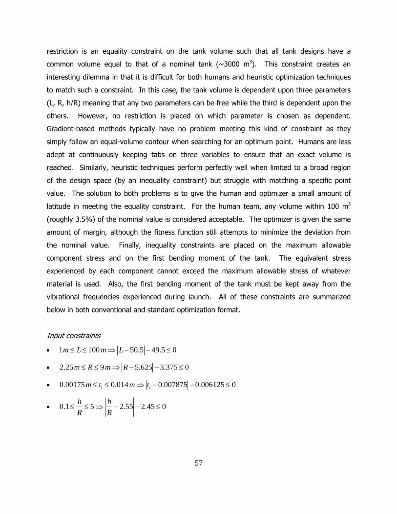
restriction is an equality constraint on the tank volume such that all tank designs have a
common volume equal to that of a nominal tank (~3000 m3). This constraint creates an
interesting dilemma in that it is difficult for both humans and heuristic optimization techniques
to match such a constraint. In this case, the tank volume is dependent upon three parameters
(L, R, h/R) meaning that any two parameters can be free while the third is dependent upon the
others. However, no restriction is placed on which parameter is chosen as dependent.
Gradient-based methods typically have no problem meeting this kind of constraint as they
simply follow an equal-volume contour when searching for an optimum point. Humans are less
adept at continuously keeping tabs on three variables to ensure that an exact volume is
reached. Similarly, heuristic techniques perform perfectly well when limited to a broad region
of the design space (by an inequality constraint) but struggle with matching a specific point
value. The solution to both problems is to give the human and optimizer a small amount of
latitude in meeting the equality constraint. For the human team, any volume within 100 m3
(roughly 3.5%) of the nominal value is considered acceptable. The optimizer is given the same
amount of margin, although the fitness function still attempts to minimize the deviation from
the nominal value. Finally, inequality constraints are placed on the maximum allowable
component stress and on the first bending moment of the tank. The equivalent stress
experienced by each component cannot exceed the maximum allowable stress of whatever
material is used. Also, the first bending moment of the tank must be kept away from the
vibrational frequencies experienced during launch. All of these constraints are summarized
below in both conventional and standard optimization format.
Input constraints
• 1 100 50.5 49.5 0m L m L≤ ≤ ⇒ − − ≤
• 2.25 9 5.625 3.375 0m R m R≤ ≤ ⇒ − − ≤
• 0.00175 0.014 0.007875 0.006125 0i im t m t≤ ≤ ⇒ − − ≤
• 0.1 5 2.55 2.45 0h hR R
≤ ≤ ⇒ − − ≤
57
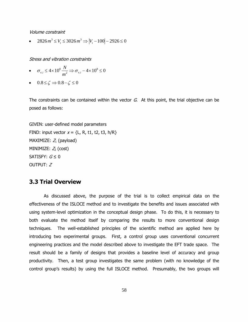
Volume constraint
• 3 32826 3026 100 2926 0t tm V m V≤ ≤ ⇒ − − ≤
Stress and vibration constraints
• 8 8, ,24 10 4 10 0e i e i
Nm
σ σ≤ × ⇒ − × ≤
• 0.8 0.8 0ζ ζ≤ ⇒ − ≤
The constraints can be contained within the vector G. At this point, the trial objective can be
posed as follows:
GIVEN: user-defined model parameters
FIND: input vector x = {L, R, t1, t2, t3, h/R}
MAXIMIZE: Z1 (payload)
MINIMIZE: Z2 (cost)
SATISFY: G ≤ 0
OUTPUT: Z
3.3 Trial Overview
As discussed above, the purpose of the trial is to collect empirical data on the
effectiveness of the ISLOCE method and to investigate the benefits and issues associated with
using system-level optimization in the conceptual design phase. To do this, it is necessary to
both evaluate the method itself by comparing the results to more conventional design
techniques. The well-established principles of the scientific method are applied here by
introducing two experimental groups. First, a control group uses conventional concurrent
engineering practices and the model described above to investigate the EFT trade space. The
result should be a family of designs that provides a baseline level of accuracy and group
productivity. Then, a test group investigates the same problem (with no knowledge of the
control group’s results) by using the full ISLOCE method. Presumably, the two groups will
58

arrive at different sets of solutions that can be compared to each other for accuracy and
completeness in terms of defining the trade space and Pareto front. The hypothesis to be
tested is that the use of background optimization will make the test group more effective
relative to the control group, given the same amount of time. The routes taken by the groups
can also be compared and ranked according to the number of designs developed, the ratio of
dominated/non-dominated designs, elapsed time, etc. After the experiment is run, this
information can be collated and analyzed to gain insight into the effectiveness of the ISLOCE
method and the role of optimization in conceptual design.
3.3.1 Specific Trial Objectives
The task presented to both groups is identical. Given the EFT model, each group
attempts to solve the multidisciplinary design optimization problem posed above within a fixed
amount of time. The end result should be an approximation of the EFT Pareto front with
designs that maximize available shuttle payload, minimize tank construction costs, and satisfy
all constraints on volume, stress, and vibration. The primary goal is to develop this
approximation with a minimum of three point designs: a maximum payload anchor point, a
minimum cost anchor point, and a compromise point somewhere between the two. This set of
points provides the minimum amount of data necessary to develop a front approximation and
perform any kind of meaningful analysis of the method performance.
The secondary goals are those that allow additional insight into the effectiveness of the
method used. These additional goals include finding multiple compromise (trade-off) points
and investigating the sensitivity of parameters on the final design. Extra compromise points are
desirable for several reasons. First, they provide a more accurate estimate of the Pareto front
(more points allow for better polynomial fits). Also, they allow for additional metrics by which
the two methods can be judged. The ratio of the number of dominated to non-dominated
solutions gives a feel for how efficiently a method produces solutions that are worth
investigating further (versus solutions that are dominated and whose discovery represents a
waste of time). Having multiple compromise points also introduces the possibility of using
59

minimum utopia point distance as a metric. A ‘best’ compromise point from each group can be
defined as the point that minimizes the normalized distance to the utopia point (i.e. the ideal
tank design that offers “infinite” payload for zero cost). This distance provides a measure of
the penetration depth of each group’s Pareto front and shows how closely they approach the
true Pareto front.
Finally, if a group does a good job in exploring the trade space of the initial problem in a
short amount of time, they have the option of attempting a second design problem. This
additional problem is similar to the first, but uses modified values of some of the internal
parameters within the EFT model. Some examples of possible parameter modifications include:
• Scaling up the seam cost-per-unit-length (e.g. representing a shortage of welding labor)
• Altering the density and cost of the tank material (representing a high-level decision to
switch materials because of cost, availability, etc.)
• Relaxing the constraint on stress or vibration (due to better structural design or more
accurate finite-element analysis
These changes are not intended to be drastic but should introduce enough change into the
model to cause a shift in Pareto-optimal designs. The purpose of making these modifications is
to determine how well a design method reacts to changes in the high-level requirements or
assumptions. Model flexibility is a highly desirable attribute that allows a design team to adapt
quickly to unforeseen changes. This ability to accommodate uncertainty goes a long way
towards alleviating project risk and helps reduce design costs.
3.3.2 Trial Procedure
The total amount of time allotted for each group was three hours. One hour was spent
learning about the EFT model and the design tools while the remaining two hours were devoted
to the design sessions. Broken down further, the schedule (in h:mm format) is as follows:
• 0:00–0:30 Trial introduction, purpose, and objectives
• 0:30–1:00 ICEMaker tutorial, EFT demo, trial goals and procedure
• 1:00–3:00 Design session and trade space exploration (additional design session optional)
• 3:00 on Post-trial debriefing and evaluation
60

The first hour was basically the same for both groups in terms of procedure with the
major differences emerging later during the sessions themselves. The trial introduction was
presented in PowerPoint with information about the trial purpose and a summary of the task.
Background information was provided about the external fuel tank and the model to be used
during the design session. Information about the model itself was presented at a level
necessary to understand and operate it without overwhelming the user (see Appendix A2).
General trends rather than specific equations were presented whenever possible. A short
description of the module and a simplified N2 chart helped all participants know what
information each module has as inputs and outputs and demonstrated the overall flow of
information.
Trial participants were also given a short introduction to the use of ICEMaker. The
instruction focused on client usage and transferring data with the ICEMaker server since this is
the primary skill required for the actual task. No training was necessary in client development,
server operation, or new parameter generation. A common vocabulary of ICEMaker terms was
established to ensure that everyone could communicate effectively during the design sessions.
Finally, participants were provided with a simplified procedure to follow during the design
sessions (see Appendix A3).
Participants were not given full information about the specifics of this thesis in order to
preserve objectivity and reduce bias. For example, participants were aware of the existence of
other groups but not of other methods. Further, no results from the design sessions were
shared between the two groups until after the conclusion of both trials. It was necessary to
explicitly emphasize to both groups that their design sessions should not be treated as a race or
competition. While it was important that they budget their allotted schedule efficiently and not
waste any time, having a competitive mindset or trying to rush through the process would be
detrimental to the results. Instead, participants were encouraged to be patient, to think about
every step in the process, and to ask questions if necessary.
61

The last part of the introduction was a trial run through the full procedure so that
participants could gain a small amount of hands-on experience using the tools before beginning
the design session. A small change was made in the input vector given to the structures chair
and this change was allowed to propagate through the system so that the team could see the
results. This process was repeated once more to confirm that everyone knew how to operate
his or her client. During this demonstration period, the author interacted briefly with each
subsystem chair regarding specific issues with that chair’s client. Any individual help needed
was given at this time to minimize observer interaction with the chair during the design session
itself. At the conclusion of the first hour, the team would be given the green light to begin its
independent evaluation of the EFT trade space and the clock was started. The author served as
an observer during the experiment taking notes on the team’s progress and answering
questions of clarification only. The next subsection describes the separate procedures followed
by each group during their respective trials.
3.3.2.1 Control Group Procedure
The control group requires four participants, one for each of the four EFT modules
(structures, aerodynamics, cost, and systems). Experience with the disciplines is not necessary
to operate the client effectively, so participants are free to choose based on personal
preference. The procedure for the control group is somewhat simpler than for the optimization
group. Without the complication of having to generate neural networks and run GAs, the
control group design session is simply a standard ICEMaker session:
1. The structures chair modifies the input vector (based on input from his model, other team
members, previous designs, and his own intuition) until he finds one that he or she believes
is a good candidate. The chair then confirms that the selected vector meets all constraints
on volume, stress, and vibration. If it passes, then the structures chair outputs his
information to the ICEMaker server. If not, then the design vector must be tweaked until all
constraints are met.
2. The aerodynamics and cost chairs request the latest information from the server and
examine the effects the chosen vector has on their subsystems. In the absence of changes
to the internal parameters of the model, these chairs’ primary job is to make observations
62

about the results of each change and to try and discern a pattern for what leads to a good
tank design. This information should feed back to the structures chair after each iteration
cycle. Once the two chairs have finished making their observations, they output their data
to the ICEMaker server.
3. The systems chair requests the latest information from the server and adds the new design
to the running table of discovered solutions. The visual depiction of the current design is
automatically updated. The new point is also plotted on the performance-versus-cost chart
and compared to previous solutions. From this information and the input of the other
subsystem chairs, a new input vector can be devised and the cycle iterates until the Pareto
front is well established or time expires.
3.3.2.2 Optimization Group Procedure
The optimization group requires four or five participants. With five participants, the
setup is the same as for the control group with the extra participant placed in charge of the
optimization module. With four participants however, the group uses a slightly different
workload distribution. The structures and systems chairs retain their previous positions, but the
aerodynamics and cost chairs are combined into a single position. This is done to free up one
member to operate the optimization chair position. This combination of positions does not
significantly alter the group dynamics, as the workload that goes into operating the two
positions is not substantial compared to that required for the structures, systems, and
optimization positions.
With access to the optimization module, the optimization group follows a different
procedure for its trial. It consists of a series of nested iterative loops:
1) At the beginning of the design session, the three main EFT modules (structures,
aerodynamics, and cost) call up the optional optimization sheet within their ICEMaker client
and initiate the neural network generation process. This takes approximately ten minutes.
Once the process is complete, the neural network data is saved in a common folder.
2) At this point, the design team breaks off into the foreground and background processes
described in the ISLOCE chapter (Chapter 2).
63

a) The conventional design team (foreground) begins exploring the trade space exactly as
described for the control group.
b) Simultaneously, the optimization chair (background) collects the neural network data
from the EFT model and uses the data to initiate a system-level optimization using a
genetic algorithm.
3) Once the GA is finished and post-processing is completed, the optimization chair
communicates the results to the rest of the team. Predicted Pareto-dominant points are
tabulated and provided to the structures chair for evaluation using the full EFT model.
4) Steps 2 and 3 can be repeated. The foreground process investigates the new points
discovered by the GA while the background process begins a new optimization run using
different parameters (possible choices for GA parameter modification include population
size, number of generations, cross-over probability, and mutation probability). Due to the
stochastic nature of GAs, this parameter modification frequently results in the discovery of
other Pareto-dominant solutions and allows the team to explore different parts of the trade
space. Again, this cycle can iterate until a desired level of completeness for the Pareto front
is reached or time expires.
It is important to note that step 1 never needs to be repeated unless some of the
internal parameters of the EFT model are changed (when examining the effects of higher
welding costs, for instance). The time spent generating the neural networks should be seen as
a one-time investment that provides the design team with information about the trade space at
the very beginning of the trial and continues to pay off periodically throughout the session.
3.4 Evaluation Metrics
The experimental framework described above as applied to evaluating different design
methods is, to the author’s knowledge, unique. Previous papers on new design methods
certainly demonstrate their power and utility, but no direct comparisons using an experimental
setup are used. It is usually left to the reader to attempt to quantify the differences between
the methods, but in the absence of a controlled environment this data is difficult to obtain. This
paper creates a first-cut attempt at developing such an environment. The preceding sections
64

describe in detail the motivation, setup, and procedure needed to perform a live test of the
ISLOCE method. However, before presenting the results of the experiment, it is necessary to
develop metrics by which the ISLOCE method can be compared to conventional design
methods.
The preferred approach would be to follow precedent and use established gauges of
performance in order to maintain consistency and allow for objective comparisons between
many different design techniques. Since no previous trials are available, a series of possible
performance measures will be described below. Both the metric and the reasoning behind it
will be given. It is hoped that future design methods will make use of them for their
comparisons.
Independent metrics
These metrics can be used to quantify the stand-alone performance of a design method.
1. Maximum/minimum objective values – These values (located at the anchor points) come
from the designs that have the ‘best’ possible value for a single objective, i.e. the global
optima. In the EFT model, the key values are maximum available payload and minimum
cost. These designs are like those that are developed using only single-objective
optimization with no regard for other objectives, but which still must satisfy all
constraints.
2. Raw number of point designs – This metric counts the total number of unique viable
point designs developed by a method. While this gives no information about the quality
of point designs (a random input vector generator would conceivably have a very high
score), it provides a general feel for how long a method takes to create a viable
solution. Combined with other metrics, this score can be used to determine average
process loop time, percentage of Pareto-dominant solutions, etc.
3. Raw number of “Pareto” optimal designs – This metric counts the number of unique
point designs that are non-dominated when compared to all the solutions generated by
a method. This metric also requires context to be interpreted correctly. It is easy to
create a splash of points with a fraction of non-dominant ones among them if none of
65
them are close to the true Pareto front. However, this metric serves as a measure of
productivity as a method explores the trade space. A larger number of predicted non-
dominated points means a greater number of points can be recommended for higher
fidelity examination.
4. Ratio of dominated to non-dominated designs – This ratio provides a measure of
method efficiency. A higher ratio implies less time is wasted discovering dominated
solutions.
5. Normalized minimum Pareto front / utopia point distance – Given a spread of point
designs, the trade space is normalized by placing the anchor points at opposite corners
(1,0) and (0,1) with the nadir and utopia points defined as (0,0) and (1,1), respectively
(for a two-objective maximization problem). This metric is defined as the shortest
distance between a point design on the Pareto front and the utopia point. The point
chosen on the Pareto front must be an actual design that satisfies all constraints and not
an interpolation of where the front could be. This metric measures the penetration
depth of a method in reaching for the ideal solution.
Comparative metrics
These metrics are best used to compare the performance of two different design methods.
1. Anchor point spread – This metric is given as the range of objective values defined by
the anchor points. It is a measure of how completely a method explores a trade space
within specified side constraints on the design vector.
2. Ratio of cross-dominated solutions – This metric takes the Pareto front of one method
and counts the number of dominated Pareto front designs generated by the other
method. The ratio of these two counts provides a measure of how much more effective
one method was over the other in approaching the true Pareto front. A ratio close to
one implies both methods are relatively equal in performance (or explored disparate
areas of the trade space). A ratio far from unity implies one method was significantly
better at getting close to the true Pareto front.
66

3.5 Live Test Results
The live test with the setup and procedures listed above was conducted in May of 2004
in the MIT Department of Aeronautics and Astronautics design studio (33-218). Eight MIT
Aero/Astro graduate students were recruited to participate in the trial. The students were
selected based on availability, familiarity with the EFT model, past experience with concurrent
engineering, knowledge of optimization basics, and personal interest in the project. The group
breakdown was as follows:
Control Group Optimization Group
Structures William Nadir Babak Cohanim
Aerodynamics Theresa Robinson Masha Ishutkina
Cost Xiang Li Masha Ishutkina
Systems Gergana Bounova Ryan Peoples
Optimization <N/A> Simon Nolet
Table 1 – Live trial participants
In addition to the participants, the author was present for both trials to deliver the
introductory presentation, run the ICEMaker demo, and make observations throughout the
design session. The control group trial was conducted first, then the optimization group trial a
week later. No information about the results of the trials was shared between groups until after
the conclusion of the second test. The results of the live tests will be presented one group at a
time and then combined in an additional section for comparative analysis.
3.5.1 Control Group Results Summary
The control group’s performance set the baseline for evaluation of the ISLOCE method. With
no access to optimization, the only trade space knowledge the group started with was a single
data point: the nominal values of a standard tank. The control group’s initial approach was to
make small perturbations to the original design vector and examine the effects on the tank’s
67

performance. During this stage, most changes were made to the tank’s geometric dimensions
with only secondary consideration paid to the component thicknesses. The result was a series
of designs that became progressively cheaper, but could not carry a significant amount of
payload due to the added weight from excessive material thickness. Later, as the team gained
more knowledge of the interaction of various parameters, they became more adept at
modifying multiple parameters at a time. They learned how to tune the component thicknesses
to the minimum values allowed by the constraints in order to achieve the lightest design
possible for a given set of geometric dimensions. This knowledge led them to the high payload
/ high cost region of the trade space. Towards the end of the design session, the control group
progressed back to the nominal design regime and completed their exploration of the trade
space in the low payload / low cost region. The results of the control group trial are listed on
the following pages in the order in which they were found. Note that point 9 is significantly
worse than all other designs and is not shown on the plot for scaling reasons.
68

1
2
3
56
8
10
11
12
13
14
15
1617
18
192320
21
222425
47
nominal
440000
480000
520000
560000
600000
640000
12000 16000 20000 24000 28000 32000 36000 40000
Available Shuttle Payload (kg)
Cos
t ($
)
Figure 18 – Control group trade space exploration
69

Design # Payload Cost Length Radius t_cy t_s t_co h/Rnominal 30000 $511,424 41.5 4.50 0.0070 0.0080 0.0075 1.0
1 24688 $500,018 40.0 4.60 0.0070 0.0090 0.0090 0.5 2 16727 $487,343 30.0 5.20 0.0090 0.0100 0.0100 0.5 3 16285 $501,558 26.0 5.50 0.0100 0.0100 0.0120 1.0 4 18205 $466,533 22.0 5.80 0.0090 0.0110 0.0100 1.0 5 19221 $449,640 20.0 5.90 0.0090 0.0105 0.0095 1.0 6 15844 $454,868 18.0 6.15 0.0095 0.0110 0.0100 1.0 7 18475 $471,703 16.0 6.15 0.0095 0.0110 0.0095 2.0 8 29800 $548,232 45.0 4.25 0.0080 0.0080 0.0070 1.5 9 2219 $716,579 40.0 4.50 0.0150 0.0150 0.0150 1.5 10 20204 $624,032 50.0 4.10 0.0100 0.0100 0.0100 1.5 11 34351 $551,885 50.0 4.10 0.0065 0.0080 0.0065 1.5 12 33509 $563,704 51.5 4.10 0.0065 0.0080 0.0065 1.5 13 32409 $535,983 45.0 4.30 0.0070 0.0080 0.0070 1.5 14 35773 $556,479 45.0 4.20 0.0065 0.0075 0.0065 3.0 15 35948 $567,545 45.0 4.15 0.0065 0.0075 0.0065 3.6 16 33712 $542,187 40.0 4.40 0.0070 0.0080 0.0070 3.0 17 30437 $534,968 35.0 4.70 0.0075 0.0085 0.0075 3.0 18 27524 $525,780 30.0 5.00 0.0080 0.0090 0.0080 3.0 19 28216 $497,903 25.0 5.20 0.0080 0.0095 0.0080 3.0 20 26148 $493,678 22.0 5.40 0.0085 0.0095 0.0085 3.0 21 26736 $498,049 23.5 5.28 0.0085 0.0095 0.0085 3.0 22 21344 $508,555 20.0 5.70 0.0090 0.0100 0.0090 3.0 23 25507 $492,148 21.0 5.48 0.0085 0.0100 0.0085 3.0 24 21416 $498,273 18.0 5.80 0.0090 0.0105 0.0090 3.0 25 18093 $495,035 14.0 6.15 0.0095 0.0110 0.0095 3.0
Table 2 – Control group point designs
3.5.2 Control Group Performance
Before applying the metrics developed in a previous section, it is important to point out
some highlights of the control group’s trial. First, the majority of solutions found by the control
group are arranged in a fairly linear pattern between the two anchor points. With the exception
of two outliers, there is very little scattering of points away from the predicted Pareto front. No
point was found which dominated the nominal solution. By following the numerical order of the
points as the team discovered them, one can trace the evolution of the design exploration over
time. Some key observations from this analysis:
70

• The first seven designs explore tanks with lengths shorter than the nominal value. Designs
1-3 carry significantly less payload without any major decrease in cost. Designs 4-7 shorten
the length even further and drive the cost down due to the decrease in material used.
• The next eight designs primarily explore tanks with lengths longer than the nominal value.
Designs 8-10 proved to be far inferior to previous designs because of their unnecessary
thicknesses (note that point 9 is not pictured on the chart as it is nowhere near the Pareto
front). The control group caught on to this trend and attempted to minimize thicknesses for
the next several solutions. As a result, Pareto dominant designs 11 and 13-15 were all
discovered quickly.
• The remaining designs slowly decreased the length again, keeping the height constant and
minimizing the thicknesses where possible. The solutions found filled in the gap between
the high payload / high cost region and the low payload / low cost region, with the final
designs ending up near the range of designs 2 and 3.
The performance metrics for the control group are summarized in the table below.
Min/Max objective values max payload = 35,948 kg min cost = $449,640
Number of point designs 26 viable designs, or roughly 13 per hour Number of “optimal” designs 10 non-dominated designs (including the
nominal point) Ratio of dominated to non-dominated solutions
10/26 or ~ 38%
Normalized minimum utopia point distance closest Pareto point to utopia: design 19 (0.538, 0.591) => 0.617 from the point (1,1)
Anchor point spread payload: {19221,35948} => 16727 cost: {449640, 567545} => 117905
Table 3 – Control group performance summary
A detailed discussion of this data will be given after the results of the optimization group are
presented.
3.5.3 Optimization Group Results Summary
The optimization group’s performance benefited significantly from access to optimization
through the ISLOCE method. Although the team’s progress was somewhat haphazard at times,
71

the overall results were an improvement over the baseline established by the control group.
The group had no problems with generating the neural networks for the optimization chair and
running genetic algorithms during the design session. This represented an initial investment
and meant that the progress of this group was initially delayed relative to the control group.
The exploration in parallel by the optimizer and the human team worked as predicted. The
optimization chair and the rest of the team complimented each other’s work by supplying each
other with data on the solutions their respective methods developed. The optimization chair
had more difficulty initially in finding viable point designs, but eventually became proficient at
generating new solutions based on the input from the optimization chair. Progress for the
optimization “group” came in waves as the optimizer provided new sets of points for exploration
by the rest of the team. Due to the stochastic nature of genetic algorithms, some predicted
Pareto fronts actually resulted in dominated designs and thus wasted time. However, the GA
was also able to point the optimization group towards regions of the trade space that the
control group did not find. The numerical results of the optimization group trial are listed on
the following pages, again, in the order in which they were discovered. Note that design 28 is
much worse than the other designs and is not shown on the plot for scaling reasons.
72

3231
30
29
2726
2524
23
2221
2019
1817
16
15
14
13
12
11
10
9
8
7
6 5
432
1
nominal
440000
480000
520000
560000
600000
640000
12000 16000 20000 24000 28000 32000 36000 40000
Available Shuttle Payload (kg)
Cos
t ($
)
Figure 19 – Optimization group trade space exploration
73

Design # Payload Cost Length Radius t_cy t_s t_co h/R nominal 30000 $511,424 41.50 4.50 0.00700 0.00800 0.00750 1.00
1 20414 $636,561 50.00 4.10 0.01000 0.01000 0.01000 2.00 2 28836 $481,042 30.43 5.00 0.00790 0.00890 0.00790 1.54 3 28709 $485,913 29.70 5.05 0.00790 0.00890 0.00790 1.79 4 29036 $491,730 30.40 4.99 0.00790 0.00890 0.00790 1.92 5 27113 $567,546 50.00 4.10 0.00790 0.00890 0.00790 1.00 6 20132 $568,309 20.00 5.30 0.01000 0.01000 0.01000 5.00 7 25116 $540,505 20.00 5.30 0.00850 0.00940 0.00850 5.00 8 23708 $609,920 32.00 4.68 0.00720 0.01000 0.01400 4.97 9 16566 $624,993 27.50 4.90 0.01000 0.01000 0.01400 4.78 10 29484 $557,806 32.70 4.70 0.00720 0.00870 0.00910 4.29 11 27802 $511,695 32.70 4.90 0.00800 0.00870 0.00910 2.00 12 16026 $598,294 55.00 4.00 0.00800 0.00870 0.01400 0.25 13 29298 $565,132 30.75 4.67 0.00710 0.00890 0.01000 4.99 14 29416 $583,020 35.00 4.50 0.00710 0.00890 0.01000 4.99 15 25626 $559,545 25.00 5.00 0.00800 0.00890 0.01000 4.99 16 20548 $471,825 25.00 5.50 0.00900 0.01000 0.01000 1.00 17 24789 $487,696 25.00 5.40 0.00850 0.00950 0.00900 2.00 18 27432 $481,221 30.58 5.00 0.00780 0.00990 0.01000 1.32 19 32105 $524,101 38.52 4.60 0.00700 0.00860 0.00700 2.16 20 33180 $526,384 39.73 4.50 0.00690 0.00860 0.00685 2.23 21 32918 $553,254 45.00 4.30 0.00690 0.00860 0.00685 2.23 22 34570 $545,937 45.00 4.30 0.00655 0.00755 0.00655 2.23 23 32153 $505,230 40.00 4.50 0.00690 0.00800 0.00830 1.30 24 31151 $511,836 42.00 4.48 0.00680 0.00785 0.00695 1.07 25 33800 $505,394 40.00 4.47 0.00680 0.00785 0.00695 1.53 26 37181 $554,732 50.00 4.05 0.00615 0.00710 0.00615 2.10 27 15173 $549,933 10.00 6.20 0.00940 0.01090 0.00950 5.00 28 1181 $539,942 10.00 7.00 0.01200 0.01400 0.01400 2.00 29 22908 $536,792 16.55 5.60 0.00850 0.00980 0.00850 4.97 30 20304 $559,528 18.43 5.41 0.00820 0.01100 0.01200 4.83 31 27797 $550,454 44.70 4.30 0.00810 0.00870 0.00880 1.32 32 26854 $542,026 50.00 4.21 0.00640 0.00820 0.00880 0.51
Table 4 – Optimization group point designs
3.5.4 Optimization Group Performance
The results of the optimization group display a very different pattern from those
generated by the control group. Whereas the control group’s data showed a linear distribution,
the optimization group’s solutions are far more scattered across the trade space. This effect is
74

due mainly to the team’s investigation of GA-supplied points that turned out to be dominated
when evaluated using the full EFT model. In terms of performance, the optimization group was
able to find points that dominated the nominal point provided at the start of the trial, as well as
most of the points found by the control group. Additional observations can be made by tracing
the path of the optimization group through the trade space.
• The first design (and others not listed due to constraint violation) represent the team’s initial
solution attempt while the first GA was still running. No improvement was made on the
nominal design until after the GA was finished.
• Designs 2-4 were recommended by the first complete GA run. The only Pareto optimal
points predicted by this run were very similar designs, hence the tight clustering of points.
This is most likely the result of the niching, or bunching up, phenomenon frequently
encountered with GAs.
• While the second GA ran with different parameters, the rest of the design team developed
designs 5-7. None of these designs were very good, but here the group began to
comprehend the value of minimizing component thicknesses.
• The second GA run produced points 8-11. For some reason, the GA thought these points
should perform much better than they do. The high cone height requires near-maximum
thickness which drives the mass up. The suspected cause of this anomaly is high sensitivity
of the neural network approximations to component thicknesses.
• Designs 12-17 were a combination of optimizer-suggested points and independently
obtained solutions. Point 16 is noteworthy because it is the low cost anchor point yet was
not hinted at by the optimizer during any of the runs. The GA did a poor job exploring the
low cost region of the trade space, though it is possible that the point would emerge
eventually using different GA settings or the introduction of restrictive mating in the GA.
• Designs 18-26 focus mostly on the high payload region of the trade space. As with the
previous GA run, some of the points (18-20 for example) are direct GA recommended points
while others (21-26) are points developed by the design team after examining the trends
predicted by the GA.
• The next four designs (27-30) were an attempt at pushing the low cost bound by
decreasing the length of the tank, but neither the team nor the GA could improve upon any
of the previous designs using this strategy.
75

• The final GA run yielded the last two points, both of which were dominated by previous
designs.
The performance metrics for the optimization group are summarized in the table below.
Min/Max objective values max payload = 37,181 kg min cost = $471,825
Number of point designs 33 viable designs, or roughly 17 per hour Number of optimal designs 7 Pareto designs
Ratio of dominated to non-dominated solutions
7/33 or ~ 21%
Normalized minimum utopia point distance closest Pareto point to utopia: design 25 (0.797, 0.595) => 0.453 from the point (1,1)
Anchor point spread payload: {20548,37181} => 16633 cost: {471825, 554732} => 82907
Table 5 – Optimization group performance summary
A performance comparison of the two groups is given in the next section.
3.5.5 Combined Results and Comparisons
The combined results of both trials provide a great deal of information, not only on the
effectiveness of the two methods but also on the benefits and issues associated with using
optimization in a concurrent engineering environment. The two primary sources for this
information are the combined results of the trade space exploration and the comparison of
metrics established in the two trials. While most of the data gleaned from the trials is
quantitative, it is equally important to investigate the qualitative data produced by the trials,
specifically from comments made by participants during the trial. As will be shown, these less-
tangible features of the two approaches can significantly contribute to a method’s performance.
76

440000
480000
520000
560000
600000
640000
12000 16000 20000 24000 28000 32000 36000 40000
Available Shuttle Payload (kg)
Cos
t ($
)
Figure 20 – Combined trade space exploration (circle: control, square: optimization)
77

Available Shuttle Payload
Cos
t
(0,0) (1,0)
(0,1) (1,1)
Figure 21 – Normalized Pareto front generated by extended GA run offline and used as “true” Pareto front (circle: control, square: optimization, diamond: Pareto)
78

Before delving into these more subjective matters, it is necessary to examine the
combined results of the two trials to put the rest of the performance discussion into proper
context. Figure 6 plots the data from figures 4 and 5 on the same axes for the purpose of
direct visual comparison of the regions explored by both methods. Two strongly dominated
outlying points are not shown for scaling purposes. In terms of finding near-Pareto optimal
designs, the optimization group’s results (in yellow) can clearly be seen to dominate those of
the control group (in green) over most regions of the trade space. The control group does a
slightly better job in the low payload / low cost region of the trade space, but it still has no
points that dominate any of the points on the optimization group Pareto front. The price the
optimization group pays for this increase in performance is also visible in the chart. The
optimization group’s points are scattered throughout the trade space, with the vast majority of
points dominated by other designs. This scattering represents ‘wasted’ time and effort by the
design team, although this time can also be seen as an investment or cost for obtaining higher
performing solutions.
Figure 7 shows the same data as the previous figure, only normalized against the two
best anchor points found during the trials. This figure provides a clearer view of what is
happening at the Pareto front. It also shows rather discontinuous nature of the front, with
large gaps in between Pareto solutions. Efforts to provide a more accurate picture of the ‘true’
Pareto front met with difficulties due to the nonlinear trade space. Several gradient-based and
heuristic attempts at plotting this front were made with limited success. Future research is
needed at better approximating the true Pareto front before archival publication. The
suspected problem is a phenomenon called “niching” where points tend to cluster during
multiobjective optimization with genetic algorithms. No anchor points could be found that were
superior to the ones found by the design teams. However, it was possible to improve on points
closer to the utopia point. The important thing to notice is that the ‘true’ Pareto front is
relatively near the one predicted by the control group and very near the front predicted by the
optimization group. This indicates that both groups were working in the correct area and were
not drastically off in their calculations.
79

The performance of the two groups can be examined further by comparing the methods
based on the metrics developed earlier. A summary of this comparison is detailed in table 6.
Control Group Optimization Group % Improvement Min/Max objective values
maximum payload 35,948 kg 37,181 kg 3.4 minimum cost $449,640 $471,825 (- 5.0) # of point designs 26 33 26.9 # of non-dominated designs
10 7 (- 30.0)
Ratio of dominated to non-dominated solutions
38% 21% (- 44.7)
Normalized minimum utopia point distance
intra-method 0.617 0.453 26.6 overall 0.678 0.563 17.0 Anchor point spread payload 16727 16633 (- 0.6) cost 117905 82907 (- 29.7)
Table 6 – Combined live trial performance metrics
These results help illustrate in more detail the visual results from figures 6-8. The
optimization group was able to locate the highest payload solution while the control group
found the point design with the lowest cost. The scale of these differences is relatively small,
but in the aerospace industry, a 3.4% boost in payload or a 5% reduction in cost can have a
major impact on the viability of a program. The anchor point spread shows that the control
group point designs cover a broader range of possible costs than do the optimization group
point designs. The optimization group was able to develop about 25% more viable point
designs than the control group. The optimization team was able to use many points directly
from the optimization run while the control group was forced to develop all of their designs
independently. However, the majority of these points were poor overall designs. The control
group had nearly double the ratio of dominated to non-dominated solutions compared the
optimization group. Much of the optimization group’s time was spent evaluating supposedly
good points recommended by the GA, only to find that most of them were dominated solutions.
The payoff from this ‘wasted’ time however is seen in the next metric. The optimization group
did a much better job at pushing their solutions closer to the utopia point. The best ‘true’
80
minimum distance found during trial post-processing was 0.520, 7% better than the best value
found by the optimization team. It should be noted that this best value was the result of a
genetic algorithm with many times more individuals and generations than the one run by the
optimization team, and consequently ran for hours rather than minutes. Even more impressive
is the fact that the optimization team was not even using the full EFT model but instead used a
series of approximations. While these results are only from a single test, if the ISLOCE method
is capable of consistently matching within 10% the performance of a full GA in a fraction of the
time, its application in industry could lead to a significant increase in the productivity of
conceptual design teams.
In addition to the quantitative data shown above, a number of more subjective
observations were made during the course of the trials. Both groups initially had difficulty
figuring out how best to go about exploring the trade space because they had no prior
knowledge of what the space looks or even what constitutes a “good” design. This problem
was obviously remedied quickly by the optimization group once the first GA run finished, but
their first attempts at generating designs were just as bad as the control group’s until the GA
came online. Another important observation made by the control group was that without any
prior knowledge it was impossible for them to ever tell if they were anywhere near the “true”
Pareto front. Over time, the control group’s confidence that they were on the right track
improved as more designs were developed, but as is shown by their results they were still
relatively far from the “true” front. Such problems did not plague the optimization group, which
was able to rapidly generate a fairly accurate picture of what the trade space looked like. The
optimization group’s confidence in the GA’s guidance had a noticeable effect on the overall
mood of the design session compared to the control group. Both groups were fortunate in that
they were only dealing with a rather simple problem with only six input variables. One can only
imagine the frustration that would be experienced by a team working on a far more complicated
problem with no additional insight as to the nature of the trade space. It is suggested that the
presence of a background optimization method can have a beneficial impact on the overall
mood and confidence level of a design team dependent upon how much trust the team places
in the optimizer’s accuracy. Repeated successful use of such a method would bolster this trust
81

and possibly lead to improvements in team morale, productivity, and consequently in the quality
of designs created. Further research on these effects is recommended.
82
4. Summary and Conclusions
4.1 Conclusions
A parallel optimization approach to concurrent engineering could offer great benefits for
any project that makes use of conceptual design. Traditionally, optimization has been
conducted by a small group of people separated from the rest of the design team. Their
models are extremely complex and may take days to run. The results from such a team are
useful but are not flexible enough to handle the rapid model changes that often occur during
concurrent engineering. This might be one of the reasons why full-scale MDO techniques have
had difficulty being infused into the mainstream design processes of major organizations. The
parallel approach presented here brings the optimization team right into the design studio,
allowing them to directly influence a design in real time while interacting with non-optimization
disciplinary specialists. The ability to quickly identify a set of interesting candidate solutions and
guide an engineering team towards them will have a significant effect on the efficiency of
design sessions.
4.2 Recommendations for Future Work
4.2.1 Refinement of Optimization Chair and Sheet Implementation The current incarnation of the optimization subsystem, while completely functional,
could greatly benefit from a number of user-friendly enhancements. The current code is run
directly at the MATLAB command line with no graphical user interface. There is also no direct
interaction with the rest of the ICEMaker clients. Other subsystems simply save their neural
networks in a common directory that the optimization chair then retrieves for incorporation into
the GA. It would be desirable to create an actual ICEMaker client for the optimization
subsystem that would interface with MATLAB through Excel Link. In this way, the optimization
83

chair would be connected to the rest of the design team while still having access to the
computing power of MATLAB. The optimization client could also output the list of interesting
point designs directly through the ICEMaker server rather than communicate it manually to the
rest of the team. Another possibility is the creation of real-time tracking and visualization of the
genetic algorithm and the evolving search space that could be projected for all to see during
the design session. Other features such as improved GA parameter control and graphing
capabilities would also be useful.
Similar improvements could be made to the optimization sheet used within the ICEMaker
clients, although this sheet is at a slightly higher level of refinement. The most important
improvement would be direct access to the neural network settings via each subsystem model.
Currently, every subsystem uses the same code to generate the neural networks. This means
that the neural network must be sized to accommodate the largest subsystem, resulting in
wasted capability for the other systems. The ability to independently tune each network
according to the needs of the associated subsystem would improve overall efficiency of the NN
generation process.
4.2.2 Comparison of CO, BLISS, and ISLOCE Each of the three major design methods discussed in this report represents a different
approach to distributed engineering and optimization. Presumably, they have specific strengths
and weaknesses when compared to each other and to more conventional design approaches. It
would be of great interest to test all three methods on a battery of standard problems and
evaluate how well each one performs. The purpose of this test would not be to determine
which method is “better” but rather to quantify the advantages and disadvantages of each.
With this information, one could select the most effective method for a problem based on the
characteristics of the expected design environment. To gather this information, a series of trials
could be run similar to the one in Chapter 3, with each method tested on a number of different
problems.
84

4.2.3 Application of ISLOCE to an Industrial Strength Problem The data collected by the live trial is the first step towards quantifying the benefits and
issues associated with ISLOCE. However, the problem used for the trial was relatively simple
and not typical of what is usually found in an industry environment. In order to validate the
advantages of ISLOCE observed during the trial, it is necessary to apply the method to high-
complexity problem, preferably with a professional organization such as JPL or General Motors.
A successful performance (or performances) under these circumstances would create a great
deal of credibility for the ISLOCE method. Regardless of the outcome, the feedback provided
by professional engineers who use the method would be invaluable in making method
improvements.
4.2.4 Background Optimization Improvements Another possible area of research is the refinement of the background. The GA used
by ISLOCE is quite basic and is limited in the types of problems can optimize. In Chapter 3, the
phenomenon of niching appeared, causing a clustering of points and a poor overall coverage of
the trade space. Improvements like restricted mating and self-tuning could solve these
problems. It is also of interest to investigate other alternatives for the background optimizer.
Simulated annealing is another heuristic optimization technique that could be employed. Any of
a number of gradient-based techniques could be tried as well.
4.2.5 Refinement of EFT Pareto Front As discussed in Chapter 3, the “true” Pareto front found by the extended GA operating
on the full EFT model demonstrated poor coverage. For comparison purposes, it is desirable to
have a fully-defined Pareto front created by a more powerful GA (or other optimization
technique). Some of the improvements described in the previous section could be used to aid
in this goal.
85

4.2.6 Trial Repetition While the results of the live trial seem to indicate that ISLOCE offers significant benefits
over design methods without optimization, the sample size for the trial is too small to make any
definitive conclusions at this point. For this reason, the live trial should be repeated with a
number of different groups to ascertain the statistical validity of the initial results. The trial
repetitions could mimic the EFT experiment exactly, or could be combined with other areas of
research such as section 4.2.2.
86

A. Appendix A1 – Space Tug Concurrent Engineering Example
This section provides an additional case study of the application of concurrent
engineering to an aerospace design problem. It also demonstrates the full use of ICEMaker in a
large group setting and serves as a good example of the end-to-end process of the ICE method.
Although the Space Tug study did not involve the ISLOCE method, it did make use of another
form of preprocessing known as multi-attribute trade space exploration, or MATE. A detailed
description of the method is included in this section as a point of comparison to ISLOCE. MATE
is similar to ISLOCE in that it uses approximation methods to perform a simplified trade space
exploration and guides the design team towards interesting candidate solutions. Whereas
ISLOCE directly incorporates the models developed by the design team, MATE is developed
independently. MATE also does not use optimization but instead relies on generating a very
large number of input vectors to completely explore the trade space.
A formal comparison of ISLOCE and MATE could be performed using the Space Tug case
study in much the same way as the EFT model was used to compare ISLOCE with conventional
concurrent engineering. The problem setup would be very similar, with one group using
ISLOCE during the design study and the other developing a MATE model to aid in the trade
space exploration. A third group could be introduced as a control to establish a baseline level
of performance for the two other teams. It is hoped that this sort of experiment could not only
provide data on the effectiveness of the two approaches but could also provide additional
reinforcement to the idea of using experimental methods to formally collect empirical data when
evaluating design methods. This sort of trial is strongly recommended as a viable area for
further research.
87

A1.1 Space Tug Introduction
An orbital transfer vehicle, or “space tug,” is one instance of a broad class of vehicles
that can perform a variety of on-orbit servicing functions. The simplest function of such a
vehicle would be to observe space assets, hereafter referred to as targets, in situ. The targets
may be cooperative (designed for servicing), partially cooperative (e.g. maneuverable in ways
helpful to the tug), uncooperative (inert), or even hostile. The latter case covers spinning or
tumbling vehicles that would be hazardous to approach. A tug changes the orbits of these
targets for operational reasons (e.g. life extension), to retrieve the targets, bringing them out of
orbit or to other assets (e.g. Shuttle or ISS), or to eliminate debris. Similar vehicles may
interact or service targets in a variety of other ways. The ability to interact with objects in
space is a desirable capability, but clearly the range of possible approaches is large, and it has
proven difficult to design viable tug systems.
The concept of tug vehicles goes back to the early years of the space program.16
Previous work has shown that hypothetical tugs designed for a single mission rarely show an
economic pay-off, although there is some evidence that if an infrastructure for on-orbit service
could be created it would have positive value.17 The concept in practice is made difficult by
unfriendly orbital dynamics (many desired maneuvers are extremely energy-intensive),
environments (the vehicle must be radiation hard, and/or hard against some level of debris
damage, to last useful lifetimes in many orbits), and economics (markets are uncertain, and
payoff is difficult to prove). Some missions require nuclear or other advanced propulsion
systems, and most require advances in control systems and docking or grappling hardware.
In this work, new space system architecture and conceptual design techniques have
been applied to the tug problem. A capability referred to as Multi-Attribute Trade space
Exploration (MATE) with Concurrent Engineering (MATE-CON) was used. MATE is a method for
examining many design concepts to understand the possibilities and problems of the space of
possible solutions – the trade space.18 It was developed at MIT from earlier work on
information systems analysis applied to space systems.19 Integrated Concurrent Engineering
(the CON in MATE-CON, but usually referred to on its own as ICE) is a method for rapidly
88

producing preliminary designs in a “design room” environment. The system used in this study
descends from work at JPL20 and the Aerospace Corporation21, by way of Caltech1. The overall
MATE-CON system, along with other front-end design tools, was developed by a consortium of
MIT, Caltech, and Stanford.22
Using MATE, several hundred possible space tug vehicles are evaluated for their ability
to move mass in orbit and interact with targets. The resulting trade space is examined to
clarify some of the fundamental difficulties with the space tug concept, understand the
sensitivities of the trade space to uncertainties in users needs, identify the Pareto front of
“good” designs, and find some design points that are promising for multi-purpose tugs. ICE is
then used to create ten conceptual designs for a range of hypothetical mission scenarios. The
ICE designs lend credibility to the crude MATE models, further clarify design issues, and provide
a starting point for further development of missions of interest.
This appendix covers the MATE and ICE models created to do the analyses, the MATE
trade space and its interpretation, and the conceptual design of four tug vehicles for a mission
involving the rescue of a Geosynchronous Earth Orbit (GEO) satellite stranded in a transfer orbit
by the failure of its apogee motor. Additional references look at a variety of specific missions,
suggested originally by this trade space analysis, that concentrate on servicing groups of
satellites in similar orbits.16
A1.2 The MATE Method
In MATE, user needs are defined in terms of the system’s attributes, or capabilities of
the desired system (objectives), rather than the characteristics of the desired space vehicle
(design vector). These needs are expressed and quantified in utility metrics, often through the
use of Multi-Attribute Utility Theory. Then a design vector is selected, consisting of a very large
number (hundreds to hundreds of thousands) of possible systems that could be used to meet
the user needs. Simulation models are used to calculate the attributes of the proposed
systems. The systems are then evaluated against the users’ utilities to understand which
systems best satisfy the users’ needs. The results, collectively referred to as the trade space,
89

can then be explored. This process consists of the search for not only optimal solutions, but
also for understanding of design sensitivities, key trade-offs, dangerous uncertainties, and
vulnerabilities to changes in the market or national policy. Often these understandings will
change a user’s perception of his or her need, and/or the designer’s perception of the
appropriate design space, resulting in a need to repeat the analysis. The semi-automated
nature of the computations allows this valuable exploitation of emergent understanding with
little cost or time penalty. Eventually, a design or designs from the trade space are selected for
further consideration.23
In this study, a somewhat simplified version of the MATE method was used. The
method was adapted in response to difficulties including the lack of an immediate customer and
a very open design space. The customer utilities were handled parametrically to understand
the sensitivities of the trade space to ranges of, and changes in, user needs. The analysis was
done at a high level, using low-fidelity models, but covering a large range of possible designs.
A1.2.1 Attributes and Utilities
The capabilities of a space tug vehicle determined to be useful to a potential user
include: (1) total delta-V capability, which determines where the space tug can go and how far
it can change the orbits of target vehicles; (2) mass of observation and manipulation equipment
(and possibly spare parts, etc.) carried, which determines at a high level what it can do to
interact with targets, referred to here as its capability; and (3) response time, or how fast it can
get to a potential target and interact with it in the desired way. Note that the design of
observation and manipulation equipment and its corresponding software is outside the scope of
this study – the equipment is treated as a “black box” with mass and power requirements.
These attributes are translated into a single utility function. In the absence of real users
from which to collect more sophisticated functions23, it was decided that a simple function that
could be explored parametrically was most appropriate. The three attributes are assigned
single-attribute utilities. These are dimensionless metrics of user satisfaction from zero
90

(minimal user need satisfied) to one (fully satisfied user). The utilities are combined as a
weighted sum.
The delta-V utility is shown in Figure. 22. Delta-V is a continuous attribute calculated for
each system considered. Utility is assumed to increase linearly with delta-V, with diminishing
returns above the levels necessary to do Low Earth Orbit (LEO) to GEO transfers. Variations on
this utility are shown in Figs. 23 and 24, which show respectively the utilities of a GEO-centric
user (large steps in utility for achieving GEO and GEO round-trip capabilities) and a delta-V-
hungry user (continued linear utility for very high delta-V). The manipulator mass (capability)
attribute has discrete values, assumed to correspond to increasing utility as shown in Table 7.
The response time of a real system would be a complex function of many factors; at the level of
the current analysis it is reduced to a binary attribute Vt, valued at one for high impulse
systems, and zero for low impulse ones.
0.00
0.10
0.20
0.30
0.40
0.50
0.60
0.70
0.80
0.90
1.00
0 2000 4000 6000 8000 10000 12000
Delta-V (m/sec)
Figure 22 – Nominal single attribute utility for ∆V
91

0.00
0.10
0.20
0.30
0.40
0.50
0.60
0.70
0.80
0.90
1.00
0 2000 4000 6000 8000 10000 12000
Delta-V (m/sec)
Figure 23 – ∆V utility for GEO-centric user
0.00
0.10
0.20
0.30
0.40
0.50
0.60
0.70
0.80
0.90
1.00
0 5000 10000 15000 20000 25000 30000 35000 40000
Delta-V (m/sec)
Figure 24 – ∆V for ∆V hungry user
92

The combined utility is calculated as follows:
Utot = WvVv +WcVc +WtVt
The combined utility is a dimensionless ranking of the presumed usefulness of the system to a
nominal user. It needs to be interpreted with care, as it provides ranking (0.8 is better than
0.4) but not scale (0.8 is not necessarily twice as good as 0.4) or any physical meaning. The
nominal weightings and two other cases studied are shown in Table 8.
A1.2.2 Design Vector and Calculation of Attributes
A set of design variables (in MATE parlance, a design vector) was selected to represent
possible tug vehicles. The following variables were selected: (1) observation and manipulator
system mass; (2) propulsion type, and (3) mass of fuel carried.
Table 7 shows the relationship assumed between manipulator mass, assumed capability,
and utility value. No attempt was made to design or even specify the manipulator system, but
for reference the 300 kg size is typical of small industrial robots, while the high capability (3000
kg) is taken from a postulated system based on shuttle arm technology.24
Table 9 shows the choices of propulsion system considered, along with some assumed
properties of the propulsion systems. The total mass of the propulsion system is taken to be
M p = mp0 + mpf M f
The fuel mass Mf was set at 30, 100, 300, 600, 1200, 3000, 10000, 30000 or 50000 kg,
obviously spanning a large range of possible delta-Vs.
93

Capability Utility value Vc
(dimensionless)
Mass Mc
(kg)
Low 0.3 300
Medium 0.6 1000
High 0.9 3000
Extreme 1.0 5000
Table 7 – Manipulator capability attribute, with corresponding utility and mass
Attribute Nominal
Weights
Capability
Stressed
Response
Time
Stressed
Delta-V 0.6 0.3 0.2
Capability 0.3 0.6 0.2
Response
Time
0.1 0.1 0.6
Table 8 – Utility weightings
Propulsion
System
Isp
(sec)
Base Mass
mp0 (kg)
Mass
Fract. mpf
High
Impulse
Storable biprop 300 0 0.12 Y
Cryo 450 0 0.13 Y
Electric 3000 25 0.30 N
Nuclear 1500 1000 0.20 Y
Table 9 – Propulsion system choices and characteristics
The design vector described above represents 144 possible designs. A few of the more
extreme of these designs were omitted, more for clarity of the resulting graphics than for
computational ease. A few designs with intermediate values of fuel mass, corresponding to
94

specific missions described in this and the companion paper, were added; the final design
vector contained 137 possible designs.
The attributes of each design were calculated as follows. The capability, and its utility,
are determined directly from the manipulator system mass as shown in Table 7. The response
time attribute is determined directly from the propulsion system choice. Those capable of high
impulse are given a response time utility Vt of one; those not capable are given a Vt of zero.
The delta-V attribute and the cost are calculated by some simple vehicle sizing rules and the
rocket equation.
The vehicle bus mass is calculated as
M b = M p + mbf M c
The vehicle dry mass is calculated as
M d = M b + M c
and the vehicle wet mass is
M w = M d + M f
The total delta-V attribute is then
∆v = g Isp ln M w M d( )
The delta-V utility is then calculated (by an interpolation routine) from Figure. 22, Figure. 23, or
Figure. 24. Note that the delta-V equation calculates the total delta-V that the vehicle can
effect on itself. Use of this value is supported by the fact that most missions studied spend
most of their fuel maneuvering the tug vehicle without an attached target. Alternately, this
delta-V can be thought of as a commodity. If a target vehicle is attached to the tug, more of
this commodity must be expended. Mission specific true delta-V’s for a variety of missions are
discussed in the references.
The individual utilities having been calculated, the total utility is calculated using the
utility equation above. The first-unit delivered cost is estimated based on a simple rule-of-
thumb formula.
C = cw M w + cd M d
95

This equation accounts for launch and first-unit hardware procurement costs. Technology
development costs are not included. The values for the coefficients in the attribute equations
are found in Tables 9 and 10. These values comprise the constants vector in MATE parlance.
The calculations are set up so that these values can be easily altered. These values were varied
+/- 10% and no strong sensitivity was found to any of them. However, it must be noted that
some of them (e.g. the nuclear propulsion properties) are quite speculative, and the trade
space may look different if they were drastically altered.
Constant Value (units)
mbf 1 (dimensionless)
cw 20 (k$/kg)
cd 150 (k$/kg)
Table 10 – Miscellaneous coefficients
A1.2.3 MATE Results
Figure 25 shows the trade space as a plot of utility vs. cost with each point representing
an evaluated design. The Pareto front of desirable designs is down (low cost) and to the right
(high performance), similar to the payload-versus-cost plots in the main body of the thesis. The
Pareto front features an area of low-cost, lower utility designs (at the bottom of Figure. 25). In
this region, a large number of designs are available, and additional utility can be had with
moderate increase in cost. On the other hand, very high levels of utility can only be purchased
at great cost (right hand side of plot).
The propulsion system is highlighted in Figure. 25, with different symbols showing
designs with different propulsion systems. The propulsion system is not a discriminator in the
low-cost, low utility part of the Pareto front, except that nuclear power is excluded. At the high
end, on the other hand, the Pareto front is populated by nuclear-powered designs. Electric
propulsion occupies the “knee” region where high utility may be obtained at moderate cost
96

97
Figure 26 shows the cost banding due to different choices of manipulator mass, or
capability. For the lower-performance systems, increased capability translates to large
increases in cost with only modest increases in utility. High capabilities are only on the Pareto
front for high utility, very high cost systems. This indicates, for the nominal set of user utilities
used, cost effective solutions would minimize the mass and power of the observation and
manipulation systems carried. Using the utility weights for the “Capability Stressed” user (Table
8) results in Figure. 27. As expected, increasing capability systems now appear all along the
Pareto front, although capability still comes at a fairly steep price.
Using the utility weightings for the “Response Time Stressed” user (Table 8) results in
Figure. 28. The results are clear; electric propulsion is eliminated from consideration. In the
nominal case (Figure. 25) electric propulsion appears at the “knee” of the Pareto front, and
would appear to give good utility for modest cost, but that conclusion will be very sensitive to
the weighting given response time by an actual user. Conversely, if the nominal weights and
the delta-V utility function from Figure. 24 are used (representing a user with a demand for
very large delta-V) the result is Figure. 29. Now, almost all the designs on the Pareto front
feature electric propulsion.

Figure 25 – Trade space for nominal user, with propulsion system indicated
Figure 26 – Trade space for nominal user, with capability indicated
98

Figure 27 – Trade space for capability stressed user
Figure 28 – Trade space for response time stressed user
99

Figure 29 – Trade space for user with large delta-V needs
Figure 30 – Low capability systems, showing effect of increasing fuel load, with GEO rescue vehicles
100

A more detailed view of the lower right-hand corner of the nominal Pareto front (from
Figure. 25) is shown in Figure. 30. Only low-capability systems are shown. The lines connect
designs that differ only by fuel load carried.
All the propulsion systems appear to hit a “wall” where costs increase sharply at little or
no advantage in utility. Examination of the designs on this wall reveal two very different
phenomena. The bi-propellant and cryogenically fueled systems are up against the limits of the
rocket equation. Each small increment in utility is gained only by carrying a lot more fuel, most
of which is used to push fuel around. The nuclear and electric systems, on the other hand, are
limited only by the fact that they achieve a high enough delta-V to score a 1.0 on the delta-V
utility, and there is simply no value in carrying more fuel. If that limit is removed, both systems
show large advantages, as shown in Figure. 29.
Also shown on Figure. 30 are some specific designs capable of carrying out the mission
mentioned in the introduction—moving from a LEO parking orbit to GEO transfer orbit,
grappling a stranded target vehicle, inserting it in GEO, and (optionally) returning to LEO. The
biprop design is “on the wall”, needing a very large fuel load to create the necessary delta-V.
The cryogenically fueled design is not as bad, but is clearly sensitive to the details of its design
– slight increases in manipulator mass etc. will send it too “up the wall.” Neither chemical fuels
can (without refueling) return a vehicle to LEO. The electric vehicles, both one-way “tug” and
round-trip “cruiser” do not have this problem. The Electric Cruiser design, in fact, sits in the
lower-right corner of the trade space because it has maximized the delta-V utility, not because
it is limited by physics.
To flesh out the vehicles briefly described here, and verify the reasonableness of the
very approximate methods used in the trade space analysis, conceptual designs for these
vehicles were created using ICE.
101

A1.3 ICE Method
A detailed description of the ICE method can be found in the main body of this thesis
(Chapter 1). This section focuses on the specific ICE model used to evaluate the Space Tug
trade space.
A1.3.1 Space Tug ICE Model
For Space Tug, each ICE session was broken down into three segments: pre-processing,
design, and post-processing. Customer inputs, payload design, and mission objectives were
decided by an Architecture chair during pre-processing. These inputs were fed to the design
team and were used to develop a point design. Finally, cost was estimated during the post-
processing segment.
Ten ICEMaker modules were developed, with each module representing a different
spacecraft subsystem or discipline. The six main modules were Mission, Systems, Propulsion,
Link, Configuration, and Power. Each sheet performed all the calculations necessary to design
its specific subsystem based on the inputs provided to it. The models were developed using
first principles whenever possible, but rules-of-thumb based on current technology were also
used to reduce complexity and coding time. These sheets were electronically linked through
the ICEMaker server and interacted throughout a design session sharing information and
updating each other of changes to the design made by the individual chairs. The ICEMaker
server works primarily with Microsoft Excel spreadsheets. This work also made innovative use
of a new software tool (Oculus CO) that was used to link routines written in Mathworks Matlab
and a parametric solid geometry model done in Solidworks® to the spreadsheets.
Several key simplifying assumptions were made. First, the sheets were only required to
handle one vehicle per design session. The Mating and Payload subsystems were treated as
“black boxes” with their specifications (mass, power, volume) fixed during the pre-processing
segment by the Architecture chair. Software, control systems, and operations were not
considered beyond a costing rule of thumb. Finally, a few aspects of the vehicle design were
handled by “dummy chairs” at a low level of model complexity. Structures, Thermal, Attitude
102

Control, and Command and Data Handling historically have a low impact on overall vehicle
design at this level of analysis and can be handled adequately by rules of thumb. These
dummy chairs can easily be expanded for future work without changing the overall architecture
if desired. The following is a summary of the six main ICEMaker modules including their inputs
and outputs:
Mission: determines delta-V requirements and other high-level specifications
• Inputs – target orbits, tasks, timeline
• Outputs – orbital elements, mission sequence, delta-Vs, lifetime, mission duration
Propulsion: sizes the propulsion subsystem, determines fuel requirements
• Inputs – initial dry mass, delta Vs, thrust requirements, target satellite masses, refueling
requirements
• Outputs – fuel mass and volume, propulsion system type with mass and power
requirements, wet mass of Space Tug
Power: sizes the power subsystem
• Inputs – power requirements (average and peak) from each subsystem by mode, orbit
periods and eclipse length by phase
• Outputs – solar array mass and area, battery and power management mass, temperature
constraints
Link: sizes the telecommunications subsystem, calculates mission link budget
• Inputs – transmit station location, Space Tug orbit parameters, uplink and downlink
margins, total data rate, mode durations
• Outputs – antenna type and dimensions, power requirements by mode, telecomm
subsystem mass
Configuration: produces a visual representation of the vehicle
• Inputs – system hardware dimensions and mass, fuel volume
• Outputs – inertia tensor, surface areas, CAD model
103

Systems: maintains summaries of all major specifications (mass, power, etc.)
• Inputs – mass by subsystem, power consumption by mode, total delta V, overall dimensions
• Outputs – total wet and dry mass by mode, link budget, cost estimate, contingencies,
margins, mission summary
A summary of the ICE model and the main module interactions are illustrated in Figure. 31.
Figure 31 – ICE model components and interactions
A full MATE-CON analysis would include the trade space analysis explicitly in the above
modeling system. In this effort, the MATE model was often run concurrently with the ICE
session, with key system parameters passed manually, so that the position of the developing
design on the trade space (as shown in Figure. 30) could be tracked in real time.
A1.3.2 ICE Results
Two main mission architectures were studied using the Space Tug ICE model: a GEO
Tug and a GEO/LEO Tender. The GEO Tug is parked in LEO and waits for a single target
mission, nominally a cooperative target of up to 2000 kg stranded in GEO transfer orbit. It then
rendezvous with the target and inserts it into a GEO orbit, and if possible returns itself to LEO.
The GEO/LEO Tender is parked in a populated, target-rich orbit and performs multiple missions
104

during its lifetime. Possible missions include moving or disposing of targets near its original
parking orbit. Both of these architectures assume a 300kg / 1kW mating device.
A1.3.2.1 GEO Tugs
Tugs were designed for both one-way and round-trip missions using three different
propulsion systems: bipropellant, cryogenic, and electric. The bipropellant and cryogenic
round-trip missions could not close their delta-V budgets, leaving four feasible designs. Table
11 and Figs. 32-34 summarize the GEO Tug designs. The masses and power figures are taken
from the ICE session results. The delta-V, utility, and cost numbers are taken from the MATE
analyses to allow direct comparison to the trade space results (e.g. Figure. 30). The ICE
system created considerably more design detail than shown in Table 11. Mass, power, and link
budgets were created—see Figure. 35 for a typical result. The physical sizes and layouts of
major components were also determined and linked to a parametric solid model, which can be
seen in Figure. 32-34. The view in Figure. 33 shows internal layout.
Design Dry Mass
(kg)
Wet Mass
(kg)
Power (w) Delta-V (km/s) Total Utility Cost
(M$)
Biprop one-way 1300 11700 1200 5.5 0.65 510
Cryo one-way 1100 6200 1200 7.1 0.69 310
Electric one-way 700 1000 3600 9.8 0.65 130
Electric cruiser 700 1100 3600 12.6 0.69 140
Table 11 – GEO Tug Design Summary
105

Figure 32 – Cryo one-way tug, showing extremely large fuel tanks; Bi-prop tug appears similar
Figure 33 – Electric Cruiser (GEO round-trip tug)
106

Figure 34 – Comparison of all GEO tug designs
Structures & Mechanisms
18%
Thermal5%
Mating System
27%
Propellant36%
Link1%
Propulsion (dry)2%
Power11%
C&DH0%
Figure 35 – Mass breakdown of Electric Cruiser design
107

The bi-prop one-way tug is very large and therefore very expensive. It is also very
sensitive to changes in any of the design assumptions; any increase in dry mass causes a very
large increase in fuel required. There is some danger that such a design would not “close” (i.e.
the required fuel mass would become infinite) if the dry mass fraction or delta-V requirements
were greater than anticipated. The best that can be said is that such a vehicle could fill a niche
for missions where a large payload must be moved quickly using existing technology.
The cryo one-way tug is significantly lighter than the biprop tug, but is almost as large
due to low fuel density. It would have a very limited life on-orbit due to the need to keep the
fuel cold. It is less sensitive to mass fractions and other assumptions, but still cannot make a
round trip to GEO.
The electric one-way and round-trip tugs seem to be practical, versatile designs with
reasonable sizes and costs. The electric designs do have the drawback of slow transit time, but
they appear to be well suited for missions where speed is not essential. The design impact of
the large total power requirement seen in Table 11 can be minimized by managing power use.
Not running the manipulator and the full thruster set all at once, and trading thruster power
(and hence impulse) vs. solar panel size results in panels not much bigger than those required
for the chemical propulsion designs (see Figs. 32 and 33).
A1.3.2.2 GEO / LEO Tenders
A family of tender missions was developed based on research of target satellite
population densities. All of the tender missions use storable bipropellant systems for reduced
cost and complexity. Each tender lives in a heavily populated orbit and is capable of performing
five or more missions involving moving or disposing of satellites near that orbit. The result of
the tender study was a line of similar vehicles with different fuel loads depending on the delta V
requirements of the desired orbit. These designs are discussed in the references.
108

A1.3.2.3 Model Consistency and Accuracy
The differences between the results of the detailed ICE and very simple MATE analyses
were remarkably small. Calculated masses differed by only a few percent. The only exceptions
were the chemical fuel one-way GEO tug designs, due to their extreme fuel loads. These
differences did not affect the points made here. Power was not calculated by the MATE model.
Delta-V was calculated differently by the ICE and MATE models, with the ICE model taking into
account the details of the mission including rendezvous maneuvers and the masses of target
vehicles, but the results were consistent given this difference. A check of the ICE models’
Theoretical First Unit (TFU) plus launch costs against the simple MATE cost model again showed
remarkable agreement (within 15% in all cases). The ICE model also included development
and engineering cost outputs, but these were not used due the wide variation in technological
maturity between the different propulsion systems considered, which the model made no
provision for.
The above comparison, along with sensitivity study carried out for the MATE analysis,
and the relative simplicity of the calculations, help verify that the models are accurate predictors
of their outputs, for the estimated or parametric inputs used. The model results should
therefore be useful for ranking and discussion, but the values given in all cases should be taken
to be estimates with accuracy appropriate for concept evaluation and comparison only.
A1.4 Case Study Observations
The trade space analyses clarify the challenges of designing space tug vehicles.
Visualization of the many possible solutions to the problem of moving mass around in near-
earth orbits reveals key constraints and trades, and concentrates attention on a set of viable
solutions. The rapid conceptual designs help to validate the crude trade space models, further
clarify design issues, and add detail and credibility to the designs of viable vehicles. The
combined set of models represents a capability that can be exercised to look at the specific
needs of customers (by identifying their utilities); exploring the possibilities of specific missions
(by designing vehicles for them, and understanding their position in the overall trade space)
109

and investigating the impact of specific technologies (by adding them to the trade space and/or
design analyses, and seeing the results).
A number of lessons that should be widely applicable to this class of vehicle were
learned during the study. First, the unfriendly physics of high delta-V missions (the “rocket
equation wall”) make carrying out these missions with chemical propulsion systems problematic.
Even if a design of this type looks feasible, it will be very vulnerable to unforeseen increases in
mass fraction and/or mission requirements, and it may be very expensive. Higher specific
impulse systems show promise, although caveats are in order. The electric propulsion systems
examined appeared to offer the best overall mix of performance and cost, but at the expense of
speed. The postulated missions are somewhat outside the current range of experience with
these technologies—it was assumed, for example, that getting operating lifetimes beyond those
of current systems would be feasible. Nuclear systems look interesting if there is need for very
high-capability systems with quick response times; they are the only technology studied that
can meet such a need. They are always expensive however, and the costs quoted here do not
include any technology development. Also, the policy and/or political issues surrounding this
technology were not addressed here. Methods for quantifying the costs of policy choices were
recently studied by Weigel25, and could be applied to this case.
The comparison of the performance of current and near future propulsion systems give
hints as to the potential value of other technologies applied to this problem. A high-Isp, high
impulse system without the large mass penalty of a nuclear system would be ideal; solar
thermal, or stored-solar-energy systems (e.g. flywheel storage) might be worth investigating for
this purpose. On the other hand, the good results with existing electric propulsion options
make other low thrust (e.g. solar sail) technologies less interesting, unless there is a very large
demand for delta-V. The trade-off between Isp, impulse, and total delta-V was found to be very
sensitive to user needs. Thus, any further discussion of the value of various propulsion systems
needs to take place in the context of the needs of a real user or at least a more completely
specified desired capability.
An issue that was relatively insensitive to user needs was the high penalty for dry mass
on the tug vehicle. The higher capability (higher observation and manipulator mass) vehicles
110

showed large cost penalties. Put another way, the total system costs were highly sensitive to
the efficiency of the observation and manipulation systems. Any user would be motivated to
achieve the highest actual capability for the lowest mass (and, secondarily, power) when
designing such equipment.
Figure 36 – Promising designs
The current trade space analysis reveals three classes of potentially useful space tug
vehicles. They are highlighted on Figure. 36. The Electric Cruiser occupies the “knee in the
curve” for our nominal utilities, providing good value for cost. It could potentially provide even
more value for a delta-V hungry user (see Figure. 29) although it is sensitive to user needs for
response time. Its features have been discussed in this paper. The “Nuclear Monsters” were
not discussed here, but appear to be the only designs (out of the design space considered) that
can provide high delta-V, high capability, rapid response systems. A final range of vehicles
occupies the lower left region of the Pareto front. These are cost effective vehicles built using
existing technology (e.g. storable bi-propellant systems) that can do a variety of jobs requiring
less delta-V than a LEO-GEO transfer. They could, for example, tend sets of vehicles in similar
orbits, doing a variety of maintenance tasks. For this reason (and to extend the naval support
vessel metaphor) they have been dubbed “Tenders.” They are considered in depth in the
references.
111

A2 – Catalog of ICEMaker and ISLOCE code The code used for all of the design sessions described in the main body of this paper
can be found on the included CD. This section contains a listing of all of the relevant files and a
short functional description. Section A3 gives a short tutorial of how to use the code to
replicate an ISLOCE design session.
A2.1 – Root Directory • ICEMaker system files
o ICEMaker.dll
o ICEMaker.chm
o ICEMaker.exe
o Project Status.xls
These files are required to initialize and run all ICEMaker sessions. They should not need to be
altered to perform any of the tasks described in this paper. Note that ICEMaker.exe is not the
file used to start the ICEMaker server, instead use ‘Shortcut to ICEMaker’ as will be described
later.
• Instructional files
o ISLOCE trial.ppt
o ISLOCE trial2.ppt
o client_howto.doc
o optimizer_howto.doc
o examples.zip
These files were used in the instruction of participants who participated in the live trial. The
first presentation was given to the control group, while the second presentation was shown to
the optimization group. The two how-to files were also provided to the optimization group to
describe the procedure for generating their neural networks and running the genetic algorithm.
The examples archive contains representative neural network and GA data for comparison
purposes.
112

A2.2 – Client Subsystems • Subsystem models
o Aerodynamics.xls
o Cost.xls
o Structures.xls
o Systems.xls
These files contain the subsystem models used for the live trial exercises. Macros must be
enabled when opening the file in order to use them during ICEMaker session.
• Other
o \Incoming
o \Template
o ISLOCE.bas
The two directories are used by ICEMaker for parameter trading and initializing new clients.
They should not need to be altered. ISLOCE.bas contains the Visual Basic code used on the
Excel side to generate the neural networks. The file can be imported as a module into any
other Excel sheet and used (in conjunction with Excel Link) to generate neural networks for
other designs.
A2.3 – Project Server • Server files and directories
o \Incoming
o ICEMaker.dat
o ICEMaker.lock
o Shortcut to ICEMaker
The Incoming directory again is used for parameter trading and tracking server requests and
should not be altered. ICEMaker.dat and .lock are storage files for the entire parameter list
being used for the active ICEMaker design. They should not be altered. The shortcut file can
be executed to launch the ICEMaker server.
113

A2.4 – Saved Session Information • \Control Group Subsystems
• \Optimization Group Subsystems
These directories contain the client models used during the live trial session in their final format.
They are provided for reference purposes only.
A2.5 – Optimization Chair • Neural network files
o GenerateNN.m
o net_aero.mat, net_cost.mat, net_struct.mat
GenerateNN is the primary Matlab file that takes the input and test data from an Excel
worksheet and launches the Neural Network toolbox to create the module approximation. The
three net files are sample neural networks generated for each of the main EFT clients.
• Genetic algorithm preparation
o convert_aero.m, convert_cost.m, convert_struct.m
o collect_nets.m
o compute_population_performance.m
o prep_genetic.m
The three convert files access the corresponding net_X.mat files and incorporate them into the
EFT performance function (compute_population_performance). Collect_nets is a scripts used to
load all of the neural networks into memory. Prep_genetic is the only file that needs to be run
in order to initialize the genetic algorithm. It contains all of the code needed to collect the
neural network data and also set the options for the GA. Some of the settings in prep_genetic
may be changed if different GA settings are desired.
• Genetic algorithm files
o b10to2.m, decode.m, encode.m, gendemo.m, genetic.m, genplot.m, mate.m,
mutate.m, reproduc.m, testgen.m, xover.m
o mdoFitness.m
o my_genetic.m
114
o Run_Me.m
The first bullet lists all of the GA function files included in the GA toolbox. These have not been
modified for the EFT session. MdoFitness.m is the fitness function passed to the genetic
algorithm to find Pareto optimal solutions. My_genetic.m is a modified version of the original
genetic.m that incorporates the use of the neural networks and also the Pareto search code.
Run_Me is a script file and is the only file that needs to be run to execute the GA once
prep_genetic has been executed.
• Post-processing files
o process_all_pop.m, determine_dominance.m
o post_proccess.m
These files perform data processing on the generated populations. Process_all_pop weeds out
all individuals that violate problem constraints. Determine_dominance singles out those points
that are Pareto superior. Post_process is a script that performs both these functions and
graphs the results. It is the only file that needs to be run after a GA is complete.
• EFT files
o EFT.m
o EFT_genetic.m
o compute_EFT_performance.m
These files were used to transfer the full EFT model directly into Matlab so that the high-level
model could be optimized to determine the true Pareto front. They are included for reference
only.
• Neural Network Storage
Various neural network trial runs are included in the NN Storage directory. Most of them do not
represent the model in its finalized form but are included for completeness.
115
A3 – ISLOCE Tutorial This section provides a step-by-step walkthrough of the procedure needed to replicate
the results of the ISLOCE trial. It is included for those who might wish to conduct further
research either on the EFT model or the method itself. A recommended strategy would be to
apply the ISLOCE method to a more complicated design problem such as the Space Tug design
described in A1 to determine whether the advantages observed during the EFT still emerge for
more complicated problems. This guide assumes that a group of participants has been
assembled and that all participants have network access to a common directory containing all of
the files described above. Optional sections are clearly marked and are for use with
optimization only.
A3.1 ICEMaker Session Initialization 1. Launch the ICEMaker server using the ‘Shortcut to ICEMaker’ file in the Project Server
directory. It is essential that no clients be run on the same computer as the server.
2. Each participant should open his or her respective ICEMaker client (aero, structures, cost,
systems). Macros must be enabled in order to pass information to and from the server.
3. (optional) Confirm that Excel Link has launched the Matlab command window and that the
active directory is set to X:\...\Optimization Chair
A3.2 Client Operation
1. Data is requested from the server by navigating to the ‘Inputs’ sheet and clicking the
‘Receive’ button.
2. Data is transferred to the server by navigating to the ‘Outputs’ sheet and clicking the ‘Send’
button.
3. (optional) A neural network for a client is generated by navigating to the ‘Optimization’
sheet and clicking the ‘CompleteNN’ button. This process will take a few minutes. Windows
will appear showing the performance of the NN when it is complete. At this point, go to the
Matlab command window and save the workspace in the active directory specified above.
a. Structures: ‘save net_struct.mat’
b. Aero: ‘save net_aero.mat’
c. Cost: ‘save net_cost.mat’
116

A3.3 Optimization Chair Operation (optional) 1. Launch Matlab and confirm that the active directory is the same as the one specified above.
2. Open prep_genetic.m and adjust settings as desired. Note that altering these values from
the default may have adverse consequences on GA performance. The following may be
modified:
a. population size
b. number of generations
c. cross-over probability
d. mutation probability
See the main body for expected results from parameter changes.
3. Run prep_genetic.m to initialize the genetic algorithm with the settings chosen.
4. Run Run_Me.m to begin the optimization process.
5. Confirm that viable solutions are being evaluated. A max fitness of 0.0001 (with the default
settings) means that no viable solutions are being generated and the GA must be restarted
with different parameters.
6. When the GA has finished, run post_process.m. This will generate plots of all viable
population members (stored in variable ‘trimmed_pop’), and all Pareto dominant individuals
(stored in variable ‘pareto_pop’). It will also display the input vectors used to create those
individuals. This information can be passed to the rest of the design team for verification
with the full EFT model.
a. Figure 1 displays all viable individuals (trimmed_pop)
b. Figure 2 displays all Pareto individuals (pareto_pop)
c. Notice that the first eight columns of pareto_pop are displayed along with the
figures. The first six columns represent the input vector (L, R, t_cyl, t_s, t_co, h/R)
and the last two are the output vector (Payload, Cost).
d. To see more individuals in this format, type:
‘display_members(trimmed_pop,<start>,<finish>,<sort_by>)’ where ‘start’ is the
starting row, ‘finish’ is the ending row, and ‘sort_by’ is the column to be sorted (7 for
payload, 8 for cost). Ex: To see members 6000 – 6050 sorted by payload, use
‘display_members(trimmed_pop,6000,6050,7)’
117
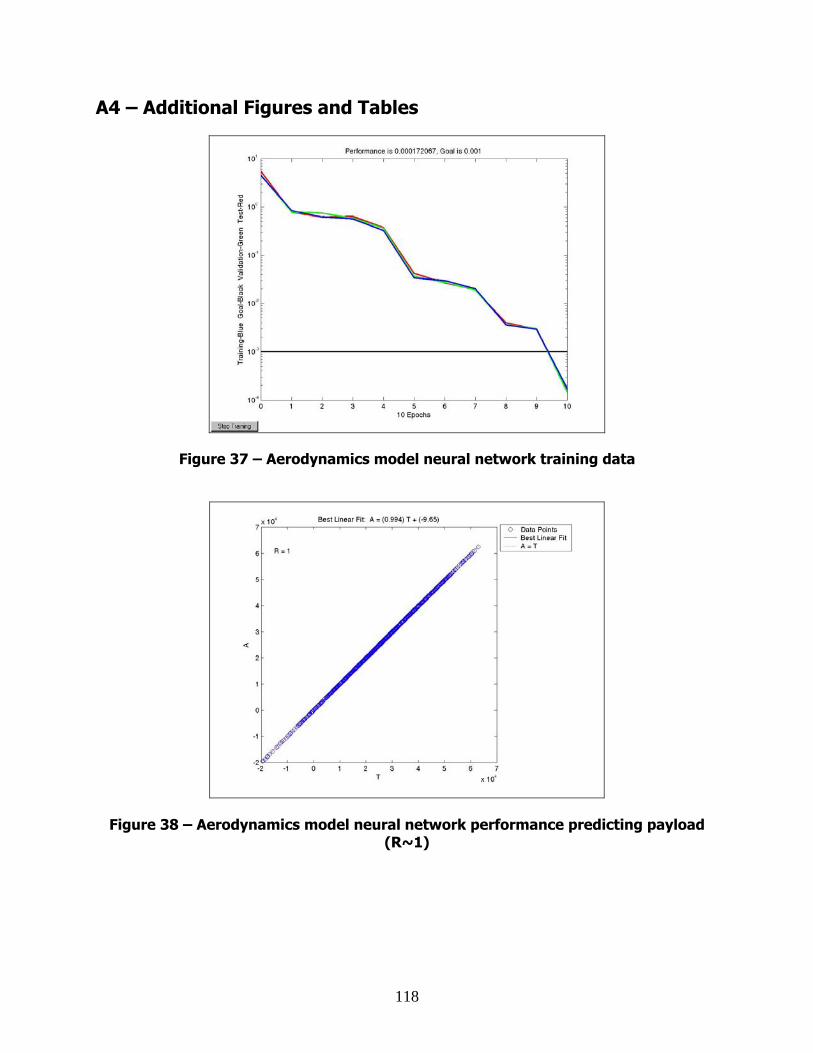
A4 – Additional Figures and Tables
Figure 37 – Aerodynamics model neural network training data
Figure 38 – Aerodynamics model neural network performance predicting payload (R~1)
118

Figure 39 – Cost model neural network training data
Figure 40 – Cost model neural network performance predicting total cost (R~1)
119

Bibliography 1 Parkin, K., Sercel, J., Liu, M., and Thunnissen, D., "ICEMaker: An Excel-Based Environment for
Collaborative Design," 2003 IEEE Aerospace Conference Proceedings, Big Sky, Montana, March
2003. Caltech Laboratory for Spacecraft and Mission Design homepage:
http://www.lsmd.caltech.edu
2 AIAA Technical Committee on Multidisciplinary Design Optimization, White Paper on Current
State of the Art, Jan. 1991.
3 Goldberg, David E. Genetic Algorithms in Search, Optimization, and Machine Learning.
Addison-Wesley Publishing Company, 1989.
4 Richards, Robert A. “Zeroth-Order Shape Optimization Utilizing a Learning Classifier System.”
Stanford University, 1995. http://www.stanford.edu/~buc/SPHINcsX/bkhm062.htm
5 Braun, R.D., “Collaborative Optimization: An Architecture for Large-Scale Distributed Design”,
Ph.D. Dissertation, Stanford University, May 1996.
6 Braun, R.D., Gage, P.J., Kroo, I.M., Sobieski, I.P., “Implementation and Performance Issues in
Collaborative Optimization”, Sixth AIAA/USAF MDO Symposium, Bellevue, WA, AIAA-94-4325,
Sept. 1996.
7 Kroo, I.M., Sobieski, I.P., “Collaborative Optimization Using Response Surface Estimation”,
AIAA #98-0915, 1993.
120

8 Sobieszczanski-Sobieski, J., Agte, J.S., Sandusky, R.R., “Bilevel Integrated System Synthesis
(BLISS)”, NASA/TM-1998-208715, August 1998b.
9 Sobieszczanski-Sobieski, J., Emiley, M.S., Agte, J., Sandusky, R., Jr. “Advancement of Bi-level
Integrated System Synthesis (BLISS)”, AIAA 2000-0421, AIAA 38th Aerospace Sciences Meeting,
Reno, Jan. 2000.
10 Demuth, Howard and Beale, Mark, Neural Network Toolbox for Use with MATLAB. The
MathWorks, Inc., 1998.
11 Kuhn, H.W., Tucker, A.W., “Nonlinear Programming”, Second Berkeley Symposium on
Mathematical Statistics and Probability. University of California Press, Berkeley. 481-492. 2.
12 Jackson, D. The Theory of Approximation. New York: American Mathematical Society, p. 76,
1930.
13 Sobieszczanski-Sobieski, J., Altus, T., Phillips, M., Sandusky, R., “Bi-Level Integrated System
Synthesis (BLISS) for Concurrent and Distributed Processing”, 9th AIAA/ISSMO Symposium on
Multidisciplinary Analysis and Optimization, Atlanta, GA., AIAA 2002-5409, Sept. 2002.
14 Sobieszczanski-Sobieski, J. “Different Objectives Result in Different Designs”. AIAA MDO
Short Course, Atlanta, GA, Sept. 2002.
15 North Carolina Foam Industries webpage: http://www.ncfi.com/space_shuttle.htm
16 Galabova, K., Bounova, G., de Weck, O. and Hastings, D., “Architecting a Family of Space
Tugs Based on Orbital transfer Mission Scenarios,” AIAA paper 2003-6368.
17 Saleh, J. H., Lamassoure, E., and Hastings, D. E. “Space Systems Flexibility Provided by On-
Orbit Servicing: Part l,” Journal of Spacecraft and Rockets, Vol. 39, No. 4, July-Aug. 2002,
pp. 551-560.
121

18 McManus, H. L., and Warmkessel, J. M., “Creating Advanced Architectures for Space Systems:
Emergent Lessons from New Processes,” Journal of Spacecraft and Rockets, in press, modified
from AIAA paper 2001-4738.
19 Shaw, G. M., Miller, D. W., and Hastings, D. E., “Development of the Quantitative Generalized
Information Network Analysis (GINA) Methodology for Satellite Systems,” Journal of Spacecraft
and Rockets, Vol. 38, No. 2, 2001, pp. 257-269.
20 Smith, J. L., “Concurrent Engineering in the JPL Project Design Center,” Society of Automotive
Engineers, Inc., Paper 98AMTC-83, 1998.
21 Aguilar, J. A., and Dawdy, A., “Scope vs. Detail: The Teams of the Concept Design Center,”
2000 IEEE Aerospace Conference Proceedings, Big Sky, Montana, March 2000, Vol. 1, pp.
465-482.
22 McManus, H. L., Hastings, D. E., and Warmkessel, J. M., “New Methods for Rapid Architecture
Selection and Conceptual Design,” Journal of Spacecraft and Rockets, in press.
23 Ross, A. M., Diller, N. P., Hastings, D. E., and Warmkessel, J. M., “Multi-Attribute Tradespace
Exploration as a Front-End for Effective Space System Design,” Journal of Spacecraft and
Rockets, in press.
24 “Project Freebird: An Orbital Transfer Vehicle”, Final report, 16.83 Space Systems
Engineering, Aeronautics and Astronautics Department, MIT, Spring 1994.
25 Weigel, A. L., and Hastings, D. E., “Evaluating the Cost and Risk Impacts of Launch Choices,”
Journal of Spacecraft and Rockets, in press.
Other References:
* Kodiyalam, S., Sobieszczanski-Sobieski, J., “Bi-Level Integrated Systems Synthesis with
Response Surfaces”, 40th AIAA/ASME/ASCE/AHS/ASC Structures, Structural Dynamics, and
Materials Conference, St. Louis, MO., Apr. 1999. AIAA 99-1306-wip
122

* Agte, J., Sobieszczanski-Sobieski, J., Sandusky, R., “Supersonic Business Jet Design Through
Bi-Level Integrated System Synthesis”, 1999 World Aviation Conference, San Francisco, CA.,
Oct. 1999. AIAA/SAE 1999-01-5622
* Rawlings, M., Balling, R., “Collaborative Optimization with Disciplinary Conceptual Design”,
AIAA-98-4919
* McManus, H., Schuman, T., “Understanding the Orbital Transfer Vehicle Trade Space”. AIAA
Space 2003 Conference, Long Beach, CA. AIAA 2003-6370, Sept. 2003.
123