IEEE TRANSACTIONS ON MAGNETICS, VOL. 51, NO. 1, JANUARY 2015 6300110

Comparison of Iron Loss Models for Electrical Machines WithDifferent Frequency Domain and Time Domain Methods

for Excess Loss PredictionDamian Kowal1, Peter Sergeant1,2, Luc Dupré1, and Lode Vandenbossche3

1Department of Electrical Energy, Systems and Automation, Ghent University, Gent B-9000, Belgium2Department of Industrial Technology and Construction, Ghent University, Gent B-9000, Belgium

3ArcelorMittal Global Research and Development Gent, Zelzate B-9060, Belgium

The goal of this paper is to investigate the accuracy of modeling the excess loss in electrical steels using a time domain model withBertotti’s loss model parameters n0 and V0 fitted in the frequency domain. Three variants of iron loss models based on Bertotti’stheory are compared for the prediction of iron losses under sinusoidal and non-sinusoidal flux conditions. The non-sinusoidalwaveforms are based on the realistic time variation of the magnetic induction in the stator core of an electrical machine, obtainedfrom a finite element-based machine model.

Index Terms— Electrical steel, excess losses, iron losses, loss modeling.

I. INTRODUCTION

AGENERAL approach for the calculation of iron loss insoft magnetic laminated materials under a unidirectional

flux φ(t) is based on the separation of the losses into threecomponents: 1) the hysteresis loss Ph ; 2) the classical loss Pc;and 3) the excess loss Pe [1]. The statistical loss theory underarbitrary flux waveforms and no minor loops is describedin [2], whereas [3] takes into account the minor order loops.Here, we may distinguish between frequency and time domainloss models.

Both frequency and time domain loss models require theidentification of certain material-dependent parameters. Forthe identification of the hysteresis loss Ph , quasi-static mea-surements of iron loss are carried out. In the case of mod-eling the classical loss Pc, when neglecting skin effect, theelectrical steel sheet-dependent parameters are the laminationthickness d and electrical conductivity σ . Both parameters areeasily measured.

In [4], the microstructural-dependent parameters describingthe excess loss component Pe are defined as n0 and V0. Bothparameters can be fitted in the frequency and time domain onthe basis of iron loss measurements for a range of frequenciesand peak induction values. The fitting method in the frequencydomain can be found in [5] and is later described in this paper.It is shown how significant is the error introduced using thematerial parameters fitted in the frequency domain to estimatethe losses in the time domain model.

The iron loss models, both frequency and time domain,exist with different levels of complexity. In this paper,we compare the loss prediction of three models with differentcomplexity, i.e., two frequency domain models and one time

Manuscript received February 6, 2014; revised May 19, 2014; acceptedJune 19, 2014. Date of publication July 11, 2014; date of currentversion January 26, 2015. Corresponding author: D. Kowal (e-mail:damian.a.kowal@gmail.com).

Color versions of one or more of the figures in this paper are availableonline at http://ieeexplore.ieee.org.

Digital Object Identifier 10.1109/TMAG.2014.2338836

domain model. The accuracy of these three different models istested both for sinusoidal and non-sinusoidal flux waveforms.A set of iron loss measurements was performed with anEpstein frame for both kinds of waveforms. The consideredmaterial is a fully processed non-oriented thin laminated,highly alloyed, low loss steel grade with a large grain size,and therefore, with a high excess loss component. Indeed, thetotal iron loss (for a time-dependent applied magnetic field)contains three components: 1) hysteresis loss; 2) classicaleddy current loss; and 3) excess loss. The hysteresis lossmay be measured by applying the same waveform for themagnetic field but at a frequency going in the limit to 0 Hzand consequently no dynamic effects are present. The classicalloss component is computed from the formulas obtained fromMaxwell’s equations and assuming a linear relation betweenthe magnetic induction and magnetic field. The excess loss ismeasured (segregated) by subtracting from the measured totaliron loss, the hysteresis and classical loss component, the lasttwo obtained as described in the previous sentences.

The choice of the non-sinusoidal flux waveforms is relatedto the estimation of the iron loss in electrical machines.Indeed, the magnetic induction waveforms in the statorteeth and yoke are non-sinusoidal, due to slot effects andnon-sinusoidal currents in the copper windings [6], [7].It is investigated how significant the loss error becomesby taking a simple frequency domain model based onthe peak value of the full waveform. This paper investi-gates also the error introduced using material related lossparameters identified from sinusoidal waveform measure-ments when the losses are estimated for a non-sinusoidalwaveform.

II. THEORETICAL ANALYSIS

A. Statistical Loss Theory for Unidirectional TimePeriodical Flux Conditions

It is well known that the dynamic losses, i.e., the clas-sical and excess losses are the result of induced electrical

0018-9464 © 2014 IEEE. Personal use is permitted, but republication/redistribution requires IEEE permission.See http://www.ieee.org/publications_standards/publications/rights/index.html for more information.

6300110 IEEE TRANSACTIONS ON MAGNETICS, VOL. 51, NO. 1, JANUARY 2015

currents due to the time varying magnetic flux appearing inthe electrical steel. According to the classical theory, wherethe material is assumed to be magnetized in a homogeneousway, these induced electrical currents are also distributed ina homogeneous way, as described by Maxwell’s equations.Due to the magnetic domain structure in electrical steels, theseinduced electrical currents are not varying in a homogeneousway in space but are located around moving magnetic domainwalls. One can attempt a general phenomenological descrip-tion of the magnetization process, where a certain numbern of active correlation regions, randomly distributed in thespecimen cross section, produce the overall observed magneticflux variation φ(t) [1]. Correlation regions are a way todescribe the fact that, given a Barkhausen jump, there is anenhanced probability that the next jump will take place in theneighborhood of the previous one. The term magnetic objectsis often used in the literature to refer to these correlationregions containing strongly interacting magnetic domain walls.Notice that φ(t) in this paper is defined as the flux in a 1 mwide lamination with thickness d .

The applied magnetic field Hs(t) (magnetic field at the sur-face of the electrical steel sheet with lamination thickness d)corresponding with the magnetic flux density B(t) in theelectrical steel sheet has a hysteresis, a classical, and anexcess field component, denoted by Hh(t), Hc(t), and He(t),respectively. Then, the instantaneous hysteresis, classical, andexcess loss components can be written as

ph(t) = Hh(t)d B

dt, pc(t) = Hc(t)

d B

dt, pe(t) = He(t)

d B

dt(1)

B(t) = φ(t)

d= 1

d

∫ d/2

−d/2Bl(x, t)dx (2)

and

Ph = 1

Tp

∫ Tp

0ph(t)dt (3)

Pc = 1

Tp

∫ Tp

0pc(t)dt (4)

Pe = 1

Tp

∫ Tp

0pe(t)dt (5)

where Bl(x, t), d , and Tp are local magnetic induction inthe sheet, thickness of the sheet, and period of the appliedmagnetic field Hs(t), respectively. The instantaneous classicalloss pc(t) is given by [1]

pc(t) = σd2

12

(d B

dt

)2

. (6)

In addition, for the instantaneous excess loss pe(t), equationscan be derived from Bertotti’s theory. When focussing on theexcess field He(t), it is shown in [1] that this field can bewritten as a function of electrical conductivity σ , the crosssection of the electrical sheet S, and the time derivative of themagnetic flux density in the electrical sheet

He(t) = σGS

n(t)

(d B

dt

). (7)

Notice that the number of simultaneously reversing magneticobjects n may vary in time and G is a dimensionless coeffi-cient [2]

G = 4

π3

∑k

1

(2k + 1)3 = 0.1356 . . . (8)

The two time-dependent functions in (7), i.e., He(t)and n(t), are not independent. In the statistical loss theoryof Bertotti, simple relations between them are postulatedand the resulting excess loss equations are then validatedexperimentally. From electromagnetic loss measurements, itbecame clear that the assumption

n(t) = n0 + He(t)

V0(9)

holds quite well for the magnetization processes underunidirectional magnetic fields for non-oriented electricalsteels and rolling direction of grain-oriented electrical steels.The material behavior under rotational field conditions is outof the scope of this paper.

From (7) and (9), one obtains for an increasing magneticflux density, by eliminating n(t)

He(t) = 1

2

(√n2

0V 20 + 4σGSV0

d B

dt− n0V0

)(10)

and consequently from (1)

pe(t) = 1

2

(√n2

0V 20 + 4σGSV0

d B

dt− n0V0

)d B

dt. (11)

From (5), (6), and (11), one may compute the classical andexcess loss for any arbitrary time-dependent periodic magneticflux pattern

Pc = σd2

12

1

Tp

∫ Tp

0

(d B

dt

)2

dt (12)

and

Pe = 1

Tp

∫ Tp

0

1

2

(√n2

0V 20 +4σGSV0

∣∣∣∣d B

dt

∣∣∣∣−n0V0

) ∣∣∣∣d B

dt

∣∣∣∣ dt .

(13)

The material parameters n0 and V0 can be derivedfrom electromagnetic loss measurements—often undersinusoidal magnetic flux conditions—at different frequenciesand induction levels as follows.

The total iron loss can then be calculated as

Pt = Ph + Pc + Pe. (14)

B. Statistical Loss Theory Under Sinusoidal Flux Patterns

In this case, a sinusoidal unidirectional flux φ(t) =d Bp sin(2π f t) or a period unidirectional flux without localminima or maxima is enforced to the electrical steel sheet nolocal minima in the induction waveform will appear (absenceof minor hysteresis loops). Therefore, it can be assumed thathysteresis loss is only related to the peak value Bp. If Wh(Bp)

KOWAL et al.: COMPARISON OF IRON LOSS MODELS FOR ELECTRICAL MACHINES 6300110

defines hysteresis energy loss per cycle for a given Bp , thenthe hysteresis power loss can be expressed as

Ph = Wh(Bp) f. (15)

Moreover, when the skin effects may be neglected, then forthe sinusoidal flux (12) reduces to

Pc = 1

6σπ2d2 B2

p f 2. (16)

According to the statistical loss theory [1], the magnetizationprocess for an arbitrary periodic magnetic flux φ(t) in a givencross section S of the lamination can be described in termsof a number of n(t) simultaneously active correlation regions,given by, see also (7)

n(t) =σGS

(d B

dt

)2

He(t)d B

dt

. (17)

One may approximate the time average of n(t) by

n = < n >≈1

Tp

∫ Tp0 σGS

( d Bdt

)2dt

1Tp

∫ Tp0 He(t)

d Bdt dt

=1

Tp

∫ Tp0 σGS

( d Bdt

)2dt

Pe. (18)

In the case of a piecewise linear time variation of B(t) withonly an absolute maximum and minimum, (18) becomes

n =< n >= 16σGSB2p f 2

Pe(19)

while in the case of a sinusoidal flux, one has

n =< n >≈ 2π2σGSB2p f 2

Pe. (20)

When defining the time averaged excess field He by

He = Pe

4Bp f(21)

we may rewrite (9) as

n = n0 + He

V0. (22)

Combining (19), (20), and (22), we obtain for the excess lossunder a piecewise linear time variation of B(t) with only anabsolute maximum and minimum

Pe = 2Bp f

(√n2

0V 20 + 16σGSV0 Bp f − n0V0

)(23)

and under a sinusoidal flux pattern

Pe = 2Bp f

(√n2

0V 20 + 2π2σGSV0 Bp f − n0V0

). (24)

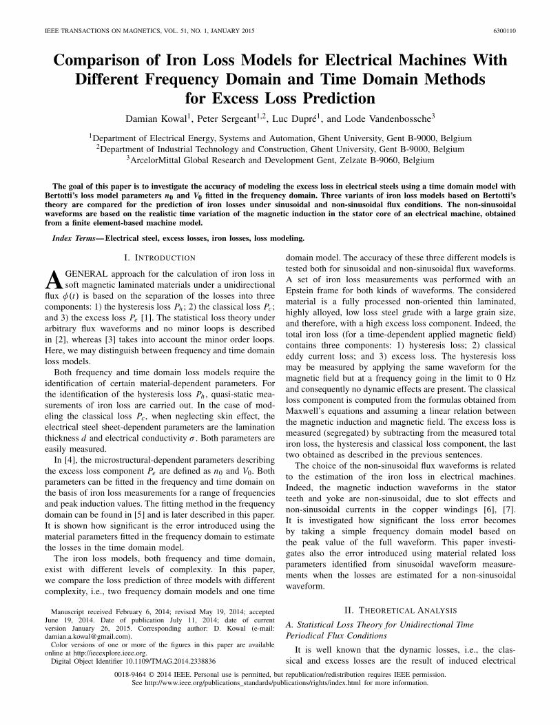
Fig. 1. Measured total loss minus classical loss versus square root offrequency. Energy loss is given per unit volume.

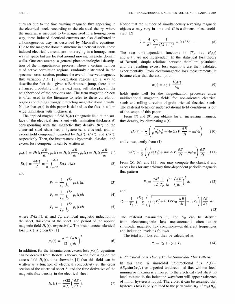
Fig. 2. Number of active correlation regions under sinusoidal flux conditions.

C. Identification of n0 and V0 Using the FrequencyDomain Approach

The identification of the microstructural-dependentparameters n0 and V0 is based on electromagnetic lossmeasurement under sinusoidal flux for different frequenciesand peak induction values.

By subtracting from the measured total loss Pt,m(Bp, f )(W/m3) the classical loss Pc(Bp, f ) given by (16), we mayconstruct (Ph + Pe)/ f as a function of the square root ofthe frequency f for the considered frequencies and inductionpeak levels (Fig. 1). By extrapolating the functions to zerofrequency, we may identify the measured hysteresis lossPh,m(Bp) (W/m3) and consequently also the measured excessloss Pe,m(Bp, f ) = Pt,m(Bp, f ) − Pc(Bp, f ) − Ph,m(Bp).

In a next step, we construct the function values n(He)for discrete values of Bp and f . Here, we make use of(20) and (21), see Fig. 2

n = 2π2σGSB2p f 2

Pe,m(25)

and

He = Pe,m

4Bp f. (26)

Notice that in Fig. 2, data is used up to 400 Hz. At thisfrequency, the considered electrical steel with a resistivity of

6300110 IEEE TRANSACTIONS ON MAGNETICS, VOL. 51, NO. 1, JANUARY 2015

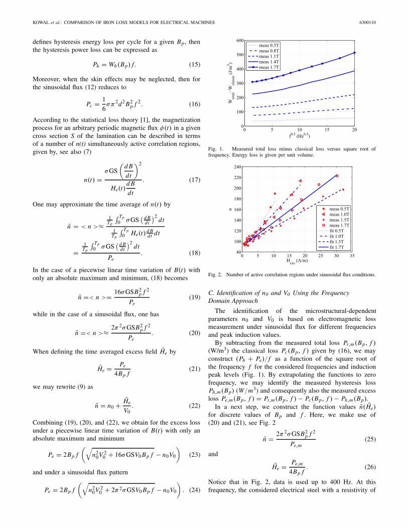
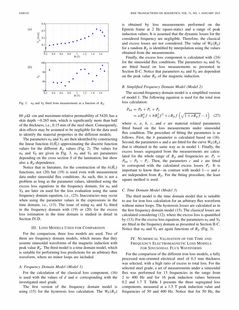
Fig. 3. n0 and V0 fitted from measurements as a function of Bp .

60 μ� · cm and maximum relative permeability of 5420, has askin depth ∼0.265 mm, which is significantly more than halfof the thickness, i.e., 0.15 mm of the steel sheet. Consequently,skin effects may be assumed to be negligible for the data usedto identify the material properties in the different models.

The parameters n0 and V0 are then identified by constructingthe linear function n(He) approximating the discrete functionvalues for the different Bp values (Fig. 2). The values forn0 and V0 are given in Fig. 3. n0 and V0 are parametersdepending on the cross section S of the lamination, but showalso a Bp-dependence.

Notice that in literature, for the construction of the n(He)functions, not (20) but (19) is used even with measurementdata under sinusoidal flux conditions. As such, this is not aproblem as long as the parameter values, identified using theexcess loss equations in the frequency domain, for n0 andV0 are later on used for the loss evaluation using the samefrequency domain equation, i.e., (23). Inaccuracies may occurwhen using the parameter values in the expressions in thetime domain, i.e., (13). The issue of using n0 and V0 fittedin the frequency domain with (19) or (20) for the excessloss estimation in the time domain is studied in detail inSection IV-D.

III. LOSS MODELS USED FOR COMPARISON

For the comparison, three loss models are used. Two ofthem are frequency domain models, which means that theyassume sinusoidal waveforms of the magnetic induction withpeak value Bp. The third model is a time domain model, whichis suitable for performing loss predictions for an arbitrary fluxwaveform, where no minor loops are included.

A. Frequency Domain Model (Model 1)

For the calculation of the classical loss component, (16)is used with the values of d and σ corresponding with theinvestigated steel grade.

The first version of the frequency domain model isusing (15) for the hysteresis loss calculation. The Wh(Bp)

is obtained by loss measurements performed on theEpstein frame at 2 Hz (quasi-static) and a range of peakinduction values. It is assumed that the dynamic losses for theconsidered frequency are negligible. Therefore, the classicaland excess losses are not considered. The value of Wh(Bp)for a random Bp is identified by interpolation using the valuesobtained from the measurements.

Finally, the excess loss component is calculated with (24)for the sinusoidal flux conditions. The parameters n0 and V0are fitted based on loss measurements as presented inSection II-C. Notice that parameters n0 and V0 are dependenton the peak value Bp of the magnetic induction.

B. Simplified Frequency Domain Model (Model 2)

The second-frequency domain model is a simplified versionof model 1. The following equation is used for the total ironloss calculation:

Ptot = Ph + Pc + Pe

= a Bαp f + bB2

p f 2 + cBp f(√

1 + eBp f − 1)

(27)

where α, a, b, c, and e are material related parametersfitted based on the loss measurements under sinusoidalflux condition. The procedure of fitting the parameters is asfollows. First, the b parameter is calculated based on (16).Second, the parameters α and a are fitted for the curve Wh(Bp)that is obtained in the same way as in model 1. Finally, theexcess losses segregated from the measurements are calcu-lated for the whole range of Bp and frequencies as: Pe =Ptot − Ph − Pc. Then, the parameters c and e are fittedto correspond with the calculated excess losses Pe. It isimportant to know that—in contrast with model 1—c and eare independent from Bp. For the fitting procedure, the leastsquare method is used.

C. Time Domain Model (Model 3)

The third model is the time domain model that is suitableto use for iron loss calculation for an arbitrary flux waveformwithout minor loops. The hysteresis losses are calculated as inthe first frequency domain model (15). The classical losses arecalculated considering (12), where the excess loss is quantifiedby (13). For the excess loss equation, the parameters n0 and V0are fitted in the frequency domain as presented in Section II-C.Notice that n0 and V0 are again functions of Bp (Fig. 3).

IV. NUMERICAL VALIDATION OF THE TIME AND

FREQUENCY ELECTROMAGNETIC LOSS MODELS

FOR SINUSOIDAL FLUX WAVEFORMS

For the comparison of the different iron loss models, a fullyprocessed non-oriented electrical steel of 0.3 mm thicknesswas selected, with a high ratio of excess to total loss. For theselected steel grade, a set of measurements under a sinusoidalflux was performed for 13 frequencies in the range from2 to 400 Hz and for 16 peak induction values between0.2 and 1.7 T. Table I presents the three segregated losscomponents, measured at a 1.5 T peak induction value andfrequencies of 50 and 400 Hz. Notice that for 50 Hz, the

KOWAL et al.: COMPARISON OF IRON LOSS MODELS FOR ELECTRICAL MACHINES 6300110

TABLE I

THREE IRON LOSS COMPONENTS SEGREGATED FROM LOSSES

MEASURED FOR 1.5 T AND A FREQUENCY OF 50 AND 400 Hz

UNDER SINUSOIDAL FLUX CONDITION (W/kg)

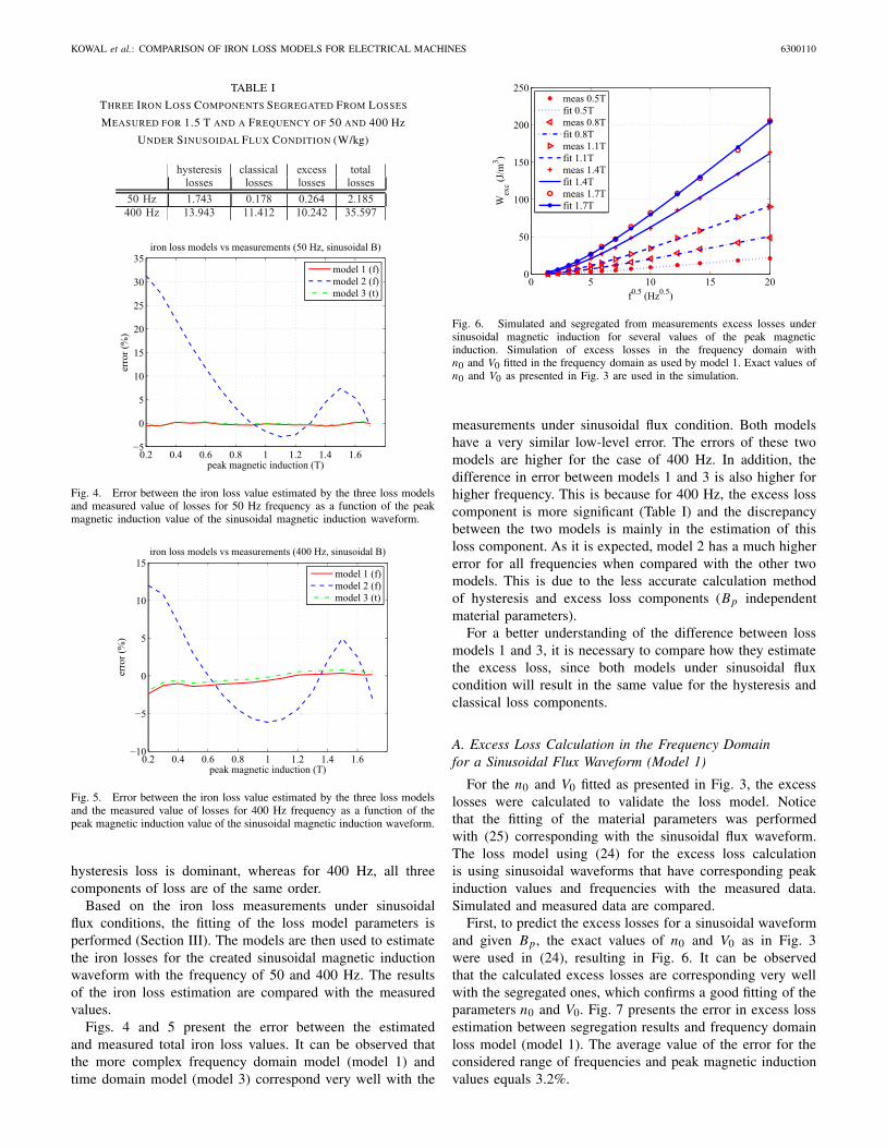
Fig. 4. Error between the iron loss value estimated by the three loss modelsand measured value of losses for 50 Hz frequency as a function of the peakmagnetic induction value of the sinusoidal magnetic induction waveform.

Fig. 5. Error between the iron loss value estimated by the three loss modelsand the measured value of losses for 400 Hz frequency as a function of thepeak magnetic induction value of the sinusoidal magnetic induction waveform.

hysteresis loss is dominant, whereas for 400 Hz, all threecomponents of loss are of the same order.

Based on the iron loss measurements under sinusoidalflux conditions, the fitting of the loss model parameters isperformed (Section III). The models are then used to estimatethe iron losses for the created sinusoidal magnetic inductionwaveform with the frequency of 50 and 400 Hz. The resultsof the iron loss estimation are compared with the measuredvalues.

Figs. 4 and 5 present the error between the estimatedand measured total iron loss values. It can be observed thatthe more complex frequency domain model (model 1) andtime domain model (model 3) correspond very well with the

Fig. 6. Simulated and segregated from measurements excess losses undersinusoidal magnetic induction for several values of the peak magneticinduction. Simulation of excess losses in the frequency domain withn0 and V0 fitted in the frequency domain as used by model 1. Exact values ofn0 and V0 as presented in Fig. 3 are used in the simulation.

measurements under sinusoidal flux condition. Both modelshave a very similar low-level error. The errors of these twomodels are higher for the case of 400 Hz. In addition, thedifference in error between models 1 and 3 is also higher forhigher frequency. This is because for 400 Hz, the excess losscomponent is more significant (Table I) and the discrepancybetween the two models is mainly in the estimation of thisloss component. As it is expected, model 2 has a much highererror for all frequencies when compared with the other twomodels. This is due to the less accurate calculation methodof hysteresis and excess loss components (Bp independentmaterial parameters).

For a better understanding of the difference between lossmodels 1 and 3, it is necessary to compare how they estimatethe excess loss, since both models under sinusoidal fluxcondition will result in the same value for the hysteresis andclassical loss components.

A. Excess Loss Calculation in the Frequency Domainfor a Sinusoidal Flux Waveform (Model 1)

For the n0 and V0 fitted as presented in Fig. 3, the excesslosses were calculated to validate the loss model. Noticethat the fitting of the material parameters was performedwith (25) corresponding with the sinusoidal flux waveform.The loss model using (24) for the excess loss calculationis using sinusoidal waveforms that have corresponding peakinduction values and frequencies with the measured data.Simulated and measured data are compared.

First, to predict the excess losses for a sinusoidal waveformand given Bp, the exact values of n0 and V0 as in Fig. 3were used in (24), resulting in Fig. 6. It can be observedthat the calculated excess losses are corresponding very wellwith the segregated ones, which confirms a good fitting of theparameters n0 and V0. Fig. 7 presents the error in excess lossestimation between segregation results and frequency domainloss model (model 1). The average value of the error for theconsidered range of frequencies and peak magnetic inductionvalues equals 3.2%.

6300110 IEEE TRANSACTIONS ON MAGNETICS, VOL. 51, NO. 1, JANUARY 2015

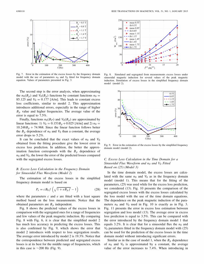
Fig. 7. Error in the estimation of the excess losses by the frequency domainmodel with the use of parameters n0 and V0 fitted for frequency domainequation. Values of parameters presented in Fig. 3.

The second step is the error analysis, when approximatingthe n0(Bp) and V0(Bp) functions by constant functions n0 =85.125 and V0 = 0.177 [A/m]. This leads to constant excessloss coefficients, similar to model 2. This approximationintroduces additional errors, especially in the range of higherBp value and higher frequencies. The average value of theerror is equal to 7.5%.

Finally, functions n0(BP) and V0(Bp) are approximated bylinear functions: 1) V0 = 0.153Bp +0.025 [A/m] and 2) n0 =10.248Bp + 74.968. Since the linear function follows betterthe Bp dependence of n0 and V0 than a constant, the averageerror drops to 5.2%.

It can be concluded that the exact values of n0 and V0obtained from the fitting procedure give the lowest error inexcess loss prediction. In addition, the better the approx-imation function corresponds with the Bp dependence ofn0 and V0, the lower the error of the predicted losses comparedwith the segregated excess losses.

B. Excess Loss Calculation in the Frequency Domainfor Sinusoidal Flux Waveform (Model 2)

The estimation of the excess losses in the simplifiedfrequency domain model is based on

Pe = cBb f(√

1 + eBp f − 1)

(28)

where the parameters c and e are fitted with a least squaremethod based on the loss measurements. Notice that theobtained parameters are Bp independent.

Fig. 8 shows the predicted values of the excess losses incomparison with the segregated ones for a range of frequenciesand few values of the peak magnetic induction. By comparingFig. 8 with Fig. 6, it is clear that the simplified model 2has much less accuracy in predicting the excess losses. Thisis also confirmed by Fig. 9, which shows the error thatmodel 2 introduces with respect to loss segregation results.The average error introduced by model 2 is 19.3%. Notice thatthe correspondence between predicted and segregated excesslosses is at its best for the middle range of frequencies, whichin this case is ∼200 Hz (Fig. 9).

Fig. 8. Simulated and segregated from measurements excess losses undersinusoidal magnetic induction for several values of the peak magneticinduction. Simulation of excess losses in the simplified frequency domainmodel (model 2).

Fig. 9. Error in the estimation of the excess losses by the simplified frequencydomain model (model 2).

C. Excess Loss Calculation in the Time Domain for aSinusoidal Flux Waveform and n0 and V0 FittedBased on (25) (Model 3)

In the time domain model, the excess losses are calcu-lated with the same n0 and V0 as in the frequency domainmodel (model 1). This means that for the fitting of theparameters, (25) was used while for the excess loss prediction,we considered (13). Fig. 10 presents the comparison of thesegregated excess losses with the excess losses calculated bythe loss model with the use of the time domain equations.The dependence on the peak magnetic induction of the para-meters n0 and V0 used in Fig. 10 is exactly as in Fig. 3.Fig. 11 presents the error in excess loss estimation betweensegregation and loss model (13). The average error in excessloss prediction is equal to 3.5%. This can be compared withthe error introduced by the frequency domain model 1 thatequals 3.2%. It is clear that for a sinusoidal flux the n0 andV0 parameters fitted in the frequency domain model with (25)can be used for the prediction of the excess losses in the timedomain model without introducing significant errors.

Similar as in the case of model 1, when the Bp dependenceof n0 and V0 is approximated by a constant, the averagevalue of the error increases to 7.4%. When introducing in

KOWAL et al.: COMPARISON OF IRON LOSS MODELS FOR ELECTRICAL MACHINES 6300110

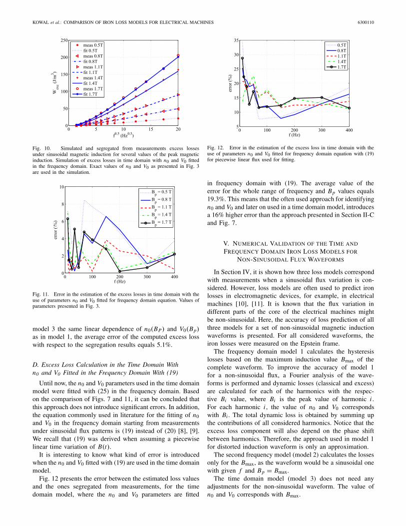
Fig. 10. Simulated and segregated from measurements excess lossesunder sinusoidal magnetic induction for several values of the peak magneticinduction. Simulation of excess losses in time domain with n0 and V0 fittedin the frequency domain. Exact values of n0 and V0 as presented in Fig. 3are used in the simulation.

Fig. 11. Error in the estimation of the excess losses in time domain with theuse of parameters n0 and V0 fitted for frequency domain equation. Values ofparameters presented in Fig. 3.

model 3 the same linear dependence of n0(BP) and V0(Bp)as in model 1, the average error of the computed excess losswith respect to the segregation results equals 5.1%.

D. Excess Loss Calculation in the Time Domain Withn0 and V0 Fitted in the Frequency Domain With (19)

Until now, the n0 and V0 parameters used in the time domainmodel were fitted with (25) in the frequency domain. Basedon the comparison of Figs. 7 and 11, it can be concluded thatthis approach does not introduce significant errors. In addition,the equation commonly used in literature for the fitting of n0and V0 in the frequency domain starting from measurementsunder sinusoidal flux patterns is (19) instead of (20) [8], [9].We recall that (19) was derived when assuming a piecewiselinear time variation of B(t).

It is interesting to know what kind of error is introducedwhen the n0 and V0 fitted with (19) are used in the time domainmodel.

Fig. 12 presents the error between the estimated loss valuesand the ones segregated from measurements, for the timedomain model, where the n0 and V0 parameters are fitted

Fig. 12. Error in the estimation of the excess loss in time domain with theuse of parameters n0 and V0 fitted for frequency domain equation with (19)for piecewise linear flux used for fitting.

in frequency domain with (19). The average value of theerror for the whole range of frequency and Bp values equals19.3%. This means that the often used approach for identifyingn0 and V0 and later on used in a time domain model, introducesa 16% higher error than the approach presented in Section II-Cand Fig. 7.

V. NUMERICAL VALIDATION OF THE TIME AND

FREQUENCY DOMAIN IRON LOSS MODELS FOR

NON-SINUSOIDAL FLUX WAVEFORMS

In Section IV, it is shown how three loss models correspondwith measurements when a sinusoidal flux variation is con-sidered. However, loss models are often used to predict ironlosses in electromagnetic devices, for example, in electricalmachines [10], [11]. It is known that the flux variation indifferent parts of the core of the electrical machines mightbe non-sinusoidal. Here, the accuracy of loss prediction of allthree models for a set of non-sinusoidal magnetic inductionwaveforms is presented. For all considered waveforms, theiron losses were measured on the Epstein frame.

The frequency domain model 1 calculates the hysteresislosses based on the maximum induction value Bmax of thecomplete waveform. To improve the accuracy of model 1for a non-sinusoidal flux, a Fourier analysis of the wave-forms is performed and dynamic losses (classical and excess)are calculated for each of the harmonics with the respec-tive Bi value, where Bi is the peak value of harmonic i .For each harmonic i , the value of n0 and V0 correspondswith Bi . The total dynamic loss is obtained by summing upthe contributions of all considered harmonics. Notice that theexcess loss component will also depend on the phase shiftbetween harmonics. Therefore, the approach used in model 1for distorted induction waveform is only an approximation.

The second frequency model (model 2) calculates the lossesonly for the Bmax, as the waveform would be a sinusoidal onewith given f and Bp = Bmax.

The time domain model (model 3) does not need anyadjustments for the non-sinusoidal waveform. The value ofn0 and V0 corresponds with Bmax.

6300110 IEEE TRANSACTIONS ON MAGNETICS, VOL. 51, NO. 1, JANUARY 2015

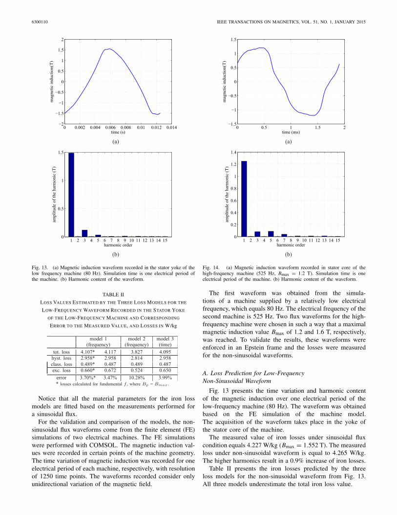
Fig. 13. (a) Magnetic induction waveform recorded in the stator yoke of thelow frequency machine (80 Hz). Simulation time is one electrical period ofthe machine. (b) Harmonic content of the waveform.

TABLE II

LOSS VALUES ESTIMATED BY THE THREE LOSS MODELS FOR THE

LOW-FREQUENCY WAVEFORM RECORDED IN THE STATOR YOKE

OF THE LOW-FREQUENCY MACHINE AND CORRESPONDING

ERROR TO THE MEASURED VALUE, AND LOSSES IN W/kg

Notice that all the material parameters for the iron lossmodels are fitted based on the measurements performed fora sinusoidal flux.

For the validation and comparison of the models, the non-sinusoidal flux waveforms come from the finite element (FE)simulations of two electrical machines. The FE simulationswere performed with COMSOL. The magnetic induction val-ues were recorded in certain points of the machine geometry.The time variation of magnetic induction was recorded for oneelectrical period of each machine, respectively, with resolutionof 1250 time points. The waveforms recorded consider onlyunidirectional variation of the magnetic field.

Fig. 14. (a) Magnetic induction waveform recorded in stator core of thehigh-frequency machine (525 Hz, Bmax = 1.2 T). Simulation time is oneelectrical period of the machine. (b) Harmonic content of the waveform.

The first waveform was obtained from the simula-tions of a machine supplied by a relatively low electricalfrequency, which equals 80 Hz. The electrical frequency of thesecond machine is 525 Hz. Two flux waveforms for the high-frequency machine were chosen in such a way that a maximalmagnetic induction value Bmax of 1.2 and 1.6 T, respectively,was reached. To validate the results, these waveforms wereenforced in an Epstein frame and the losses were measuredfor the non-sinusoidal waveforms.

A. Loss Prediction for Low-FrequencyNon-Sinusoidal Waveform

Fig. 13 presents the time variation and harmonic contentof the magnetic induction over one electrical period of thelow-frequency machine (80 Hz). The waveform was obtainedbased on the FE simulation of the machine model.The acquisition of the waveform takes place in the yoke ofthe stator core of the machine.

The measured value of iron losses under sinusoidal fluxcondition equals 4.227 W/kg (Bmax = 1.552 T). The measuredloss under non-sinusoidal waveform is equal to 4.265 W/kg.The higher harmonics result in a 0.9% increase of iron losses.

Table II presents the iron losses predicted by the threeloss models for the non-sinusoidal waveform from Fig. 13.All three models underestimate the total iron loss value.

KOWAL et al.: COMPARISON OF IRON LOSS MODELS FOR ELECTRICAL MACHINES 6300110

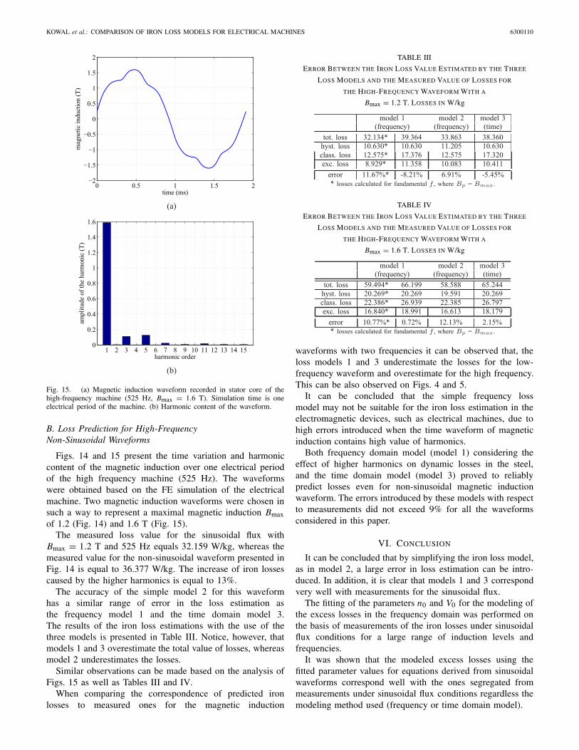
Fig. 15. (a) Magnetic induction waveform recorded in stator core of thehigh-frequency machine (525 Hz, Bmax = 1.6 T). Simulation time is oneelectrical period of the machine. (b) Harmonic content of the waveform.

B. Loss Prediction for High-FrequencyNon-Sinusoidal Waveforms

Figs. 14 and 15 present the time variation and harmoniccontent of the magnetic induction over one electrical periodof the high frequency machine (525 Hz). The waveformswere obtained based on the FE simulation of the electricalmachine. Two magnetic induction waveforms were chosen insuch a way to represent a maximal magnetic induction Bmaxof 1.2 (Fig. 14) and 1.6 T (Fig. 15).

The measured loss value for the sinusoidal flux withBmax = 1.2 T and 525 Hz equals 32.159 W/kg, whereas themeasured value for the non-sinusoidal waveform presented inFig. 14 is equal to 36.377 W/kg. The increase of iron lossescaused by the higher harmonics is equal to 13%.

The accuracy of the simple model 2 for this waveformhas a similar range of error in the loss estimation asthe frequency model 1 and the time domain model 3.The results of the iron loss estimations with the use of thethree models is presented in Table III. Notice, however, thatmodels 1 and 3 overestimate the total value of losses, whereasmodel 2 underestimates the losses.

Similar observations can be made based on the analysis ofFigs. 15 as well as Tables III and IV.

When comparing the correspondence of predicted ironlosses to measured ones for the magnetic induction

TABLE III

ERROR BETWEEN THE IRON LOSS VALUE ESTIMATED BY THE THREE

LOSS MODELS AND THE MEASURED VALUE OF LOSSES FOR

THE HIGH-FREQUENCY WAVEFORM WITH A

Bmax = 1.2 T. LOSSES IN W/kg

TABLE IV

ERROR BETWEEN THE IRON LOSS VALUE ESTIMATED BY THE THREE

LOSS MODELS AND THE MEASURED VALUE OF LOSSES FOR

THE HIGH-FREQUENCY WAVEFORM WITH A

Bmax = 1.6 T. LOSSES IN W/kg

waveforms with two frequencies it can be observed that, theloss models 1 and 3 underestimate the losses for the low-frequency waveform and overestimate for the high frequency.This can be also observed on Figs. 4 and 5.

It can be concluded that the simple frequency lossmodel may not be suitable for the iron loss estimation in theelectromagnetic devices, such as electrical machines, due tohigh errors introduced when the time waveform of magneticinduction contains high value of harmonics.

Both frequency domain model (model 1) considering theeffect of higher harmonics on dynamic losses in the steel,and the time domain model (model 3) proved to reliablypredict losses even for non-sinusoidal magnetic inductionwaveform. The errors introduced by these models with respectto measurements did not exceed 9% for all the waveformsconsidered in this paper.

VI. CONCLUSION

It can be concluded that by simplifying the iron loss model,as in model 2, a large error in loss estimation can be intro-duced. In addition, it is clear that models 1 and 3 correspondvery well with measurements for the sinusoidal flux.

The fitting of the parameters n0 and V0 for the modeling ofthe excess losses in the frequency domain was performed onthe basis of measurements of the iron losses under sinusoidalflux conditions for a large range of induction levels andfrequencies.

It was shown that the modeled excess losses using thefitted parameter values for equations derived from sinusoidalwaveforms correspond well with the ones segregated frommeasurements under sinusoidal flux conditions regardless themodeling method used (frequency or time domain model).

6300110 IEEE TRANSACTIONS ON MAGNETICS, VOL. 51, NO. 1, JANUARY 2015

It can be concluded that by approximating the dependenceof n0 and V0 on the magnetic induction level by a constantor linear function is introducing an error in modeling theexcess losses, when compared with the ones segregated frommeasurements. The approximation by a linear function intro-duces a smaller error than in the case of an approximation bya constant.

For the estimation of iron losses for non-sinusoidalwaveforms, both frequency, which considering harmonics(Fourier analysis) and time domain models can be used withrather high accuracy.

REFERENCES

[1] G. Bertotti, Hysteresis in Magnetism, for Physicists, Material Scientists,and Engineers. San Diego, CA, USA: Academic, 1998.

[2] F. Fiorillo and A. Novikov, “An improved approach to power losses inmagnetic laminations under nonsinusoidal induction waveform,” IEEETrans. Magn., vol. 26, no. 5, pp. 2904–2910, Sep. 1990.

[3] E. Barbisio, F. Fiorillo, and C. Ragusa, “Predicting lossin magnetic steels under arbitrary induction waveform and with minorhysteresis loops,” IEEE Trans. Magn., vol. 40, no. 4, pp. 1810–1819,Jul. 2004.

[4] G. Bertotti, “Physical interpretation of eddy current losses in ferromag-netic materials. II. Analysis of experimental results,” J. Appl. Phys.,vol. 57, no. 6, pp. 2110–2126, 1985.

[5] D. Kowal, P. Sergeant, L. Dupré, and A. Van den Bossche, “Comparisonof nonoriented and grain-oriented material in an axial flux permanent-magnet machine,” IEEE Trans. Magn., vol. 46, no. 2, pp. 279–285,Feb. 2010.

[6] K. Yamazaki and N. Fukushima, “Iron-loss modeling for rotatingmachines: Comparison between Bertotti’s three-term expression and3-D eddy-current analysis,” IEEE Trans. Magn., vol. 46, no. 8,pp. 3121–3124, Aug. 2010.

[7] A. M. Knight, J. C. Salmon, and J. Ewanchuk, “Integration of a firstorder eddy current approximation with 2D FEA for prediction of PWMharmonic losses in electrical machines,” IEEE Trans. Magn., vol. 49,no. 5, pp. 1957–1960, May 2013.

[8] L. R. Dupré, G. Bertotti, and J. A. A. Melkebeek, “Dynamic Preisachmodel and energy dissipation in soft magnetic materials,” IEEE Trans.Magn., vol. 34, no. 4, pp. 1168–1170, Jul. 1998.

[9] L. Dupré, G. Bertotti, V. Basso, F. Fiorillo, and J. Melkebeek,“Generalisation of the dynamic Preisach model toward grain orientedFe–Si alloys,” Phys. B, vol. 275, nos. 1–3, pp. 202–206, 2000.

[10] B. Gaussens et al., “Uni- and bidirectional flux variation locimethod for analytical prediction of iron losses in doubly-salient field-excited switched-flux machines,” IEEE Trans. Magn., vol. 49, no. 7,pp. 4100–4103, Jul. 2013.

[11] A. Belahcen, P. Rasilo, and A. Arkkio, “Segregation of iron losses fromrotational field measurements and application to electrical machine,”IEEE Trans. Magn., vol. 50, no. 2, pp. 893–896, Feb. 2014.