arX

iv:1

402.

6763

v1 [

mat

h.O

C]

27

Feb

2014

Linear Programming for Large-Scale Markov Decision Problems

Yasin Abbasi-Yadkori

Queensland University of Technology

yasin.abbasiyadkori@qut.edu.au

Peter L. Bartlett

UC Berkeley and QUT

bartlett@eecs.berkeley.edu

Alan Malek

UC Berkeley

malek@eecs.berkeley.edu

February 28, 2014

Abstract

We consider the problem of controlling a Markov decision process (MDP) with a large state

space, so as to minimize average cost. Since it is intractable to compete with the optimal

policy for large scale problems, we pursue the more modest goal of competing with a low-

dimensional family of policies. We use the dual linear programming formulation of the MDP

average cost problem, in which the variable is a stationary distribution over state-action pairs,

and we consider a neighborhood of a low-dimensional subset of the set of stationary distributions

(defined in terms of state-action features) as the comparison class. We propose two techniques,

one based on stochastic convex optimization, and one based on constraint sampling. In both

cases, we give bounds that show that the performance of our algorithms approaches the best

achievable by any policy in the comparison class. Most importantly, these results depend on

the size of the comparison class, but not on the size of the state space. Preliminary experiments

show the effectiveness of the proposed algorithms in a queuing application.

1 Introduction

We study the average loss Markov decision process problem. The problem is well-understood when

the state and action spaces are small (Bertsekas, 2007). Dynamic programming (DP) algorithms,

such as value iteration (Bellman, 1957) and policy iteration (Howard, 1960), are standard techniques

to compute the optimal policy. In large state space problems, exact DP is not feasible as the

computational complexity scales quadratically with the number of states.

A popular approach to large-scale problems is to restrict the search to the linear span of a small

number of features. The objective is to compete with the best solution within this comparison class.

Two popular methods are Approximate Dynamic Programming (ADP) and Approximate Linear

1

Programming (ALP). This paper focuses on ALP. For a survey on theoretical results for ADP see

(Bertsekas and Tsitsiklis, 1996, Sutton and Barto, 1998), (Bertsekas, 2007, Vol. 2, Chapter 6), and

more recent papers (Sutton et al., 2009b,a, Maei et al., 2009, 2010).

Our aim is to develop methods that find policies with performance guaranteed to be close to

the best in the comparison class but with computational complexity that does not grow with the

size of the state space. All prior work on ALP either scales badly or requires access to samples

from a distribution that depends on the optimal policy.

This paper proposes a new algorithm to solve the Approximate Linear Programming problem

that is computationally efficient and does not require knowledge of the optimal policy. In particular,

we introduce new proof techniques and tools for average cost MDP problems and use these tech-

niques to derive a reduction to stochastic convex optimization with accompanying error bounds.

We also propose a constraint sampling technique and obtain performance guarantees under an

additional assumption on the choice of features.

1.1 Notation

Let X and A be positive integers. Let X = {1, 2, . . . ,X} and A = {1, 2, . . . , A} be state and action

spaces, respectively. Let ∆S denote probability distributions over set S. A policy π is a map from

the state space to ∆A: π : X → ∆A. We use π(a|x) to denote the probability of choosing action a

in state x under policy π. A transition probability kernel (or transition kernel) P : X × A → ∆X

maps from the direct product of the state and action spaces to ∆X . Let Pπ denote the probability

transition kernel under policy π. A loss function is a bounded real-valued function over state and

action spaces, ℓ : X × A → [0, 1]. Let Mi,: and M:,j denote ith row and jth column of matrix M

respectively. Let ‖v‖1,c =∑

i ci |vi| and ‖v‖∞,c = maxi ci |vi| for a positive vector c. We use 1 and

0 to denote vectors with all elements equal to one and zero, respectively. We use ∧ and ∨ to denote

the minimum and the maximum, respectively. For vectors v and w, v ≤ w means element-wise

inequality, i.e. vi ≤ wi for all i.

1.2 Linear Programming Approach to Markov Decision Problems

Under certain assumptions, there exist a scalar λ∗ and a vector h∗ ∈ RX that satisfy the Bellman

optimality equations for average loss problems,

λ∗ + h∗(x) = mina∈A

[ℓ(x, a) +

∑

x′∈X

P(x,a),x′h∗(x′)

].

The scalar λ∗ is called the optimal average loss, while the vector h∗ is called a differential value

function. The action that minimizes the right-hand side of the above equation is the optimal action

in state x and is denoted by a∗(x). The optimal policy is defined by π∗(a∗(x)|x) = 1. Given ℓ and

2

P , the objective of the planner is to compute the optimal action in all states, or equivalently, to

find the optimal policy.

The MDP problem can also be stated in the LP formulation (Manne, 1960),

maxλ,h

λ , (1)

s.t. B(λ1+ h) ≤ ℓ+ Ph ,

where B ∈ {0, 1}XA×X is a binary matrix such that the ith column has A ones in rows 1+ (i− 1)A

to iA. Let vπ be the stationary distribution under policy π and let µπ(x, a) = vπ(x)π(a|x). We can

write

π∗ = argminπ

∑

x∈X

vπ(x)∑

a∈A

π(a|x)ℓ(x, a)

= argminπ

∑

(x,a)∈X×A

µπ(x, a)ℓ(x, a) = argminπ

µ⊤π ℓ .

In fact, the dual of LP (1) has the form of

minµ∈RXA

µ⊤ℓ , (2)

s.t. µ⊤1 = 1, µ ≥ 0, µ⊤(P −B) = 0 .

The objective function, µ⊤ℓ, is the average loss under stationary distribution µ. The first two

constraints ensure that µ is a probability distribution over state-action space, while the last con-

straint ensures that µ is a stationary distribution. Given a solution µ, we can obtain a policy via

π(a|x) = µ(x, a)/∑

a′∈A µ(x, a′).

1.3 Approximations for Large State Spaces

The LP formulations (1) and (2) are not practical for large scale problems as the number of vari-

ables and constraints grows linearly with the number of states. Schweitzer and Seidmann (1985)

propose approximate linear programming (ALP) formulations. These methods were later im-

proved by de Farias and Van Roy (2003a,b), Hauskrecht and Kveton (2003), Guestrin et al. (2004),

Petrik and Zilberstein (2009), Desai et al. (2012). As noted by Desai et al. (2012), the prior work

on ALP either requires access to samples from a distribution that depends on optimal policy or

assumes the ability to solve an LP with as many constraints as states. (See Section 2 for a more

detailed discussion.) Our objective is to design algorithms for very large MDPs that do not require

knowledge of the optimal policy.

In contrast to the aforementioned methods, which solve the primal ALPs (with value functions

as variables), we work with the dual form (2) (with stationary distributions as variables). Analogous

3

to ALPs, we control the complexity by limiting our search to a linear subspace defined by a small

number of features. Let d be the number of features and Φ be a (XA)× d matrix with features as

column vectors. By adding the constraint µ = Φθ, we get

minθθ⊤Φ⊤ℓ ,

s.t. θ⊤Φ⊤1 = 1, Φθ ≥ 0, θ⊤Φ⊤(P −B) = 0 .

If a stationary distribution µ0 is known, it can be added to the linear span to get the ALP

minθ

(µ0 +Φθ)⊤ℓ , (3)

s.t. (µ0 +Φθ)⊤1 = 1, µ0 +Φθ ≥ 0, (µ0 +Φθ)⊤(P −B) = 0 .

Although µ0 +Φθ might not be a stationary distribution, it still defines a policy1

πθ(a|x) =[µ0(x, a) + Φ(x,a),:θ]+∑a′ [µ0(x, a

′) + Φ(x,a′),:θ]+, (4)

We denote the stationary distribution of this policy µθ which is only equal to µ0 +Φθ if θ is in the

feasible set.

1.4 Problem definition

With the above notation, we can now be explicit about the problem we are solving.

Definition 1 (Efficient Large-Scale Dual ALP). For an MDP specified by ℓ and P , the efficient

large-scale dual ALP problem is to produce parameters θ such

µ⊤θℓ ≤ min

{µ⊤θ ℓ : θ feasible for (3)

}+O(ǫ) (5)

in time polynomial in d and 1/ǫ. The model of computation allows access to arbitrary entries of Φ,

ℓ, P , µ0, P⊤Φ, and 1⊤Φ in unit time.

Importantly, the computational complexity cannot scale with X and we do not assume any

knowledge of the optimal policy. In fact, as we shall see, we solve a harder problem, which we

define as follows.

Definition 2 (Expanded Efficient Large-Scale Dual ALP). Let V : ℜd → ℜ+ be some “violation

function” that represents how far µ0+Φθ is from a valid stationary distribution, satisfying V (θ) = 0

if θ is a feasible point for the ALP (3). The expanded efficient large-scale dual ALP problem is to

1We use the notation [v]− = v ∧ 0 and [v]+ = v ∨ 0.

4

produce parameters θ such that

µ⊤θℓ ≤ min

{µ⊤θ ℓ+

1

ǫV (θ) : θ ∈ ℜd

}+O(ǫ), (6)

in time polynomial in d and 1/ǫ, under the same model of computation as in Definition 1.

Note that the expanded problem is strictly more general as guarantee (6) implies guarantee

(5). Also, many feature vectors Φ may not admit any feasible points. In this case, the dual ALP

problem is trivial, but the expanded problem is still meaningful.

Having access to arbitrary entries of the quantities in Definition 1 arises naturally in many

situations. In many cases, entries of P⊤Φ are easy to compute. For example, suppose that for any

state x′ there are a small number of state-action pairs (x, a) such that P (x′|x, a) > 0. Consider

Tetris; although the number of board configurations is large, each state has a small number of

possible neighbors. Dynamics specified by graphical models with small connectivity also satisfy

this constraint. Computing entries of P⊤Φ is also feasible given reasonable features. If a feature ϕi

is a stationary distribution, then P⊤ϕi = B⊤ϕi. Otherwise, it is our prerogative to design sparse

feature vectors, hence making the multiplication easy. We shall see an example of this setting later.

1.5 Our Contributions

In this paper, we introduce an algorithm that solves the expanded efficient large-scale dual ALP

problem under a (standard) assumption that any policy converges quickly to its stationary distri-

bution.

Our algorithm take as input a constant S and an error tolerance ǫ, and has access to the various

products listed in Definition 1. Define Θ = {θ : θ⊤Φ⊤1 = 1 − µ⊤0 1, ‖θ‖ ≤ S}. If no stationary

distribution is known, we can simply choose µ0 = 0. The algorithm is based on stochastic convex

optimization. We prove that for any δ ∈ (0, 1), after O(1/ǫ4) steps of gradient descent, the algorithm

finds a vector θ ∈ Θ such that, with probability at least 1− δ,

µ⊤θℓ ≤µ⊤θ ℓ+

1

ǫ‖[µ0 +Φθ]−‖1 +

1

ǫ

∥∥∥(P −B)⊤(µ0 +Φθ)∥∥∥1+O(ǫ log(1/δ))

holds for all θ ∈ Θ; i.e., we solve the expanded problem for V (θ) equal to the L1 error of the

violation. The second and third terms are zero for feasible points (points in the intersection of

the feasible set of LP (2) and the span of the features). For points outside the feasible set, these

terms measure the extent of constraint violations for the vector µ0 + Φθ, which indicate how well

stationary distributions can be represented by the chosen features.

The above performance bound scales with 1/ǫ that can be large when the feasible set is empty

and ǫ is very small. We propose a second approach and show that this dependence can be eliminated

if we have extra information about the MDP. Our second approach is based on the constraint

5

sampling method that is already applied to large-scale linear programming and MDP problems

(de Farias and Van Roy, 2004, Calafiore and Campi, 2005, Campi and Garatti, 2008). We obtain

performance bounds, but under the condition that a suitable function that controls the size of

constraint violations is available. Our proof technique is different from previous work and gives

stronger performance bounds.

Our constraint sampling method takes two extra inputs: functions v1 and v2 that specify the

amount of constraint violations that we tolerate at each state-action pair. The algorithm samples

O(dǫ log1ǫ ) constraints and solves the sampled LP problem. Let θ denote the solution of the sampled

ALP and θ∗ denote the solution of the full ALP subject to constraints v1 and v2. We prove that

with high probability,

ℓ⊤µθ≤ ℓ⊤µθ∗ +O(ǫ+ ‖v1‖1 + ‖v2‖1) .

2 Related Work

de Farias and Van Roy (2003a) study the discounted version of the primal form (1). Let c ∈ RX

be a vector with positive components and γ ∈ (0, 1) be a discount factor. Let L : RX → RX be

the Bellman operator defined by (LJ)(x) = mina∈A(ℓ(x, a)+γ∑

x′∈X P(x,a),x′J(x′)) for x ∈ X . Let

Ψ ∈ RX×d be a feature matrix. The exact and approximate LP problems are as follows:

maxJ∈RX

c⊤J , maxw∈Rd

c⊤Ψw ,

s.t. LJ ≥ J , s.t. LΨw ≥ Ψw .

which can also be written as

maxJ∈RX

c⊤J , maxw∈Rd

c⊤Ψw , (7)

s.t. ∀(x, a), ℓ(x, a) + γP(x,a),:J ≥ J(x) , s.t. ∀(x, a), ℓ(x, a) + γP(x,a),:Ψw ≥ (Ψw)(x) .

The optimization problem on the RHS is an approximate LP with the choice of J = Ψw. Let

Jπ(x) = E[∑∞

t=0 γtℓ(xt, π(xt))|x0 = x

]be value of policy π, J∗ be the solution of LHS, and πJ(x) =

argmina∈A(ℓ(x, a)+γP(x,a),:J) be the greedy policy with respect to J . Let ν ∈ ∆X be a probability

distribution and define µπ,ν = (1 − γ)ν⊤(I − γP π)−1. de Farias and Van Roy (2003a) prove that

for any J satisfying the constraints of the LHS of (7),

‖JπJ− J∗‖1,ν ≤ 1

1− γ‖J − J∗‖1,µπJ ,ν

. (8)

Define βu = γmaxx,a∑

x′ P(x,a),x′u(x′)/u(x). Let U = {u ∈ RX : u ≥ 1, u ∈ span(Ψ), βu < 1}. Let

6

w∗ be the solution of ALP. de Farias and Van Roy (2003a) show that for any u ∈ U ,

‖J∗ −Ψw∗‖1,c ≤2c⊤u

1− βuminw

‖J∗ −Ψw‖∞,1/u . (9)

This result has a number of limitations. First, solving ALP can be computationally expensive as

the number of constraints is large. Second, it assumes that the feasible set of ALP is non-empty.

Finally, Inequality (8) implies that c = µπΨw∗,ν is an appropriate choice to obtain performance

bounds. However, w∗ itself is function of c and is not known before solving ALP.

de Farias and Van Roy (2004) propose a computationally efficient algorithm that is based on

a constraint sampling technique. The idea is to sample a relatively small number of constraints

and solve the resulting LP. Let N ⊂ Rd be a known set that contains w∗ (solution of ALP). Let

µVπ,c(x) = µπ,c(x)V (x)/(µ⊤π,cV ) and define the distribution ρVπ,c(x, a) = µVπ,c(x)/A. Let δ ∈ (0, 1)

and ǫ ∈ (0, 1). Let βu = γmaxx∑

x′ P(x,π∗(x)),x′u(x′)/u(x) and

D =(1 + βV )µ

⊤π∗,cV

2c⊤J∗supw∈N

‖J∗ −Ψw‖∞,1/V , m ≥ 16AD

(1− γ)ǫ

(d log

48AD

(1− γ)ǫ+ log

2

δ

).

Let S be a set of m random state-action pairs sampled under ρVπ∗,c. Let w be a solution of the

following sampled LP:

maxw∈Rd

c⊤Ψw ,

s.t. w ∈ N , ∀(x, a) ∈ S, ℓ(x, a) + γP(x,a),:Ψw ≥ (Ψw)(x) .

de Farias and Van Roy (2004) prove that with probability at least 1− δ, we have

‖J∗ −Ψw‖1,c ≤ ‖J∗ −Ψw∗‖1,c + ǫ ‖J∗‖1,c .

This result has a number of limitations. First, vector µπ∗,c (that is used in the definition of D)

depends on the optimal policy, but an optimal policy is what we want to compute in the first

place. Second, we can no longer use Inequality (8) to obtain a performance bound (a bound on

‖JπΨw− J∗‖1,c), as Ψw does not necessarily satisfy all constraints of ALP.

Desai et al. (2012) study a smoothed version of ALP, in which slack variables are introduced

that allow for some violation of the constraints. Let D′ be a violation budget. The smoothed ALP

(SALP) has the form of

maxw,s

c⊤Ψw , maxw,s

c⊤Ψw − 2µ⊤π∗,cs

1− γ,

s.t. Ψw ≤ LΨw + s, µ⊤π∗,cs ≤ D′, s ≥ 0, s.t. Ψw ≤ LΨw + s, s ≥ 0 .

7

The ALP on RHS is equivalent to LHS with a specific choice of D′. Let U = {u ∈ RX : u ≥ 1}

be a set of weight vectors. Desai et al. (2012) prove that if w∗ is a solution to above problem, then

‖J∗ −Ψw∗‖1,c ≤ infw,u∈U

‖J∗ −Ψw‖∞,1/u

(c⊤u+

2(µ⊤π∗,cu)(1 + βu)

1− γ

).

The above bound improves (9) as U is larger than U and RHS in the above bound is smaller than

RHS of (9). Further, they prove that if η is a distribution and we choose c = (1−γ)η⊤(I−γP πΨw∗ ),

then

∥∥JµΨw∗− J∗

∥∥1,η

≤ 1

1− γ

(inf

w,u∈U‖J∗ −Ψw‖∞,1/u

(c⊤u+

2(µ⊤π∗,νu)(1 + βu)

1− γ

)).

Similar methods are also proposed by Petrik and Zilberstein (2009). One problem with this result

is that c is defined in terms of w∗, which itself depends on c. Also, the smoothed ALP formulation

uses π∗ which is not known. Desai et al. (2012) also propose a computationally efficient algorithm.

Let S be a set of S random states drawn under distribution µπ∗,c. Let N ′ ⊂ Rd be a known set

that contains the solution of SALP. The algorithm solves the following LP:

maxw,s

c⊤Ψw − 2

(1− γ)S

∑

x∈S

s(x) ,

s.t. ∀x ∈ S, (Ψw)(x) ≤ (LΨw)(x) + s(x), s ≥ 0, w ∈ N ′ .

Let w be the solution of this problem. Desai et al. (2012) prove high probability bounds on

the approximation error ‖J∗ −Ψw‖1,c. However, it is no longer clear if a performance bound

on ‖J∗ − JπΨw‖1,c can be obtained from this approximation bound.

Next, we turn our attention to average cost ALP, which is a more challenging problem and is

also the focus of this paper. Let ν be a distribution over states, u : X → [1,∞), η > 0, γ ∈ [0, 1],

P πγ = γP π + (1 − γ)1ν⊤, and Lγh = minπ(ℓπ + P π

γ h). de Farias and Van Roy (2006) propose the

following optimization problem:

minw,s1,s2

s1 + ηs2 , (10)

s.t. LγΨw −Ψw + s11+ s2u ≥ 0, s2 ≥ 0 .

Let (w∗, s1,∗, s2,∗) be the solution of this problem. Define the mixing time of policy π by

τπ = inf

{τ :

∣∣∣∣∣1

t

t−1∑

t′=0

ν⊤(P π)t′

ℓπ − λπ

∣∣∣∣∣ ≤τ

t, ∀t}.

Let τ∗ = lim infδ→0{τπ : λπ ≤ λ∗ + δ}. Let π∗γ be the optimal policy when discount factor is

8

γ. Let πγ,w be the greedy policy with respect to Ψw when discount factor is γ, µ⊤γ,π = (1 −γ)∑∞

t=0 γtν⊤(P π)t and µγ,w = µγ,πγ,w . de Farias and Van Roy (2006) prove that if η ≥ (2 −

γ)µ⊤γ,π∗γu,

λw∗− λ∗ ≤

(1 + β)ηmax(D′′, 1)

1− γminw

∥∥h∗γ −Ψw∥∥∞,1/u

+ (1− γ)(τ∗ + τπw∗) ,

where β = maxπ ‖I − γP π‖∞,1/u, D′′ = µ⊤γ,w∗

V/(ν⊤V ) and V = LγΨw∗ − Ψw∗ + s1,∗1 + s2,∗u.

Similar results are obtained more recently by Veatch (2013).

An appropriate choice for vector ν is ν = µγ,w∗. Unfortunately, w∗ depends on ν. We should

also note that solving (10) can be computationally expensive. de Farias and Van Roy (2006) pro-

pose constraint sampling techniques similar to (de Farias and Van Roy, 2004), but no performance

bounds are provided.

Wang et al. (2008) study ALP (3) and show that there is a dual form for standard value function

based algorithms, including on-policy and off-policy updating and policy improvement. They also

study the convergence of these methods, but no performance bounds are shown.

3 A Reduction to Stochastic Convex Optimization

In this section, we describe our algorithm as a reduction from Markov decision problems to stochas-

tic convex optimization. The main idea is to convert the ALP (3) into an unconstrained optimiza-

tion over Θ by adding a function of the constraint violations to the objective, then run stochastic

gradient descent with unbiased estimated of the gradient.

For a positive constant H, form the following convex cost function by adding a multiple of the

total constraint violations to the objective of the LP (3):

c(θ) = ℓ⊤(µ0 +Φθ) +H ‖[µ0 +Φθ]−‖1 +H∥∥∥(P −B)⊤(µ0 +Φθ)

∥∥∥1

= ℓ⊤(µ0 +Φθ) +H ‖[µ0 +Φθ]−‖1 +H∥∥∥(P −B)⊤Φθ

∥∥∥1

= ℓ⊤(µ0 +Φθ) +H∑

(x,a)

∣∣[µ0(x, a) + Φ(x,a),:θ]−∣∣+H

∑

x′

∣∣∣(P −B)⊤:,x′Φθ∣∣∣ .

(11)

We justify using this surrogate loss as follows. Suppose we find a near optimal vector θ such that

c(θ) ≤ minθ∈Θ c(θ) +O(ǫ). We will prove

1. that∥∥∥[µ0 +Φθ]−

∥∥∥1and

∥∥∥(P −B)⊤(µ0 +Φθ)∥∥∥1are small and µ0 + Φθ is close to µ

θ(by

Lemma 2 in Section 3), and

2. that ℓ⊤(µ0 +Φθ) ≤ minθ∈Θ c(θ) +O(ǫ).

9

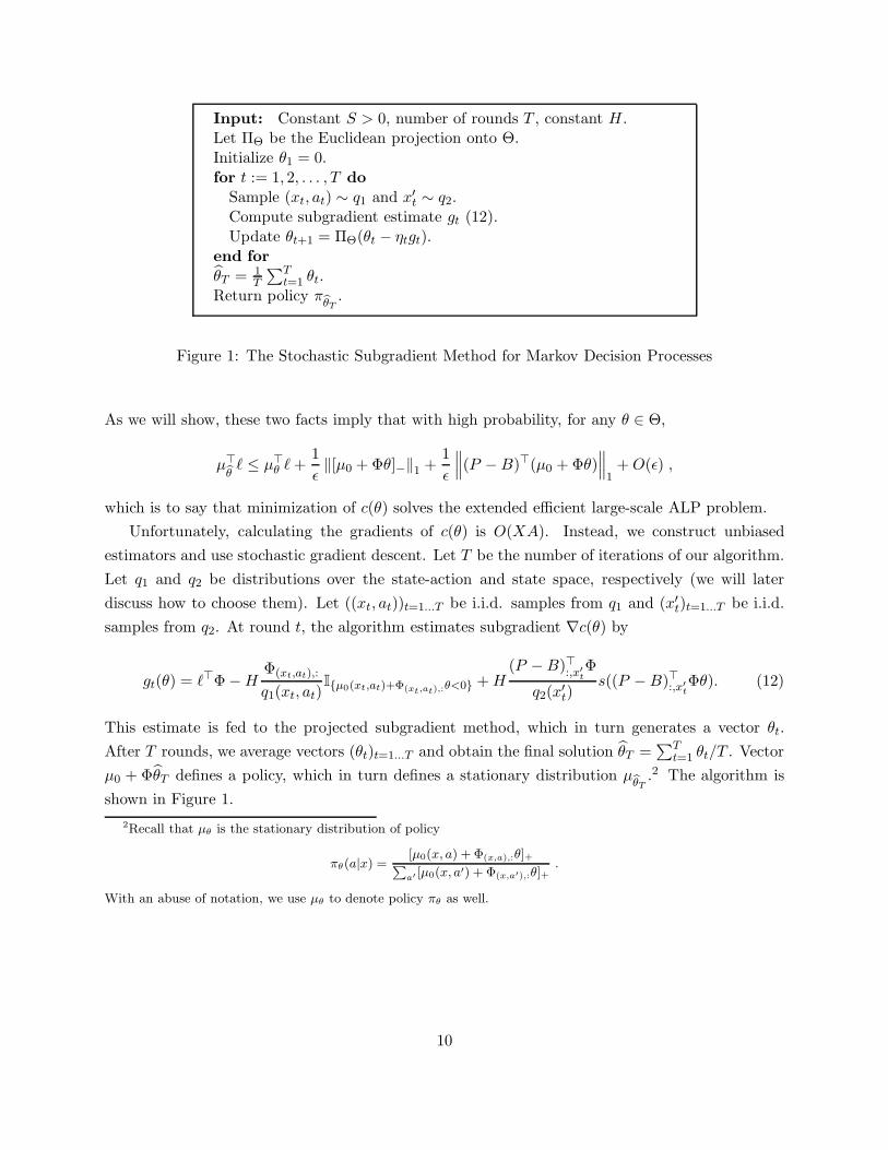
Input: Constant S > 0, number of rounds T , constant H.Let ΠΘ be the Euclidean projection onto Θ.Initialize θ1 = 0.for t := 1, 2, . . . , T do

Sample (xt, at) ∼ q1 and x′t ∼ q2.Compute subgradient estimate gt (12).Update θt+1 = ΠΘ(θt − ηtgt).

end for

θT = 1T

∑Tt=1 θt.

Return policy πθT.

Figure 1: The Stochastic Subgradient Method for Markov Decision Processes

As we will show, these two facts imply that with high probability, for any θ ∈ Θ,

µ⊤θℓ ≤ µ⊤θ ℓ+

1

ǫ‖[µ0 +Φθ]−‖1 +

1

ǫ

∥∥∥(P −B)⊤(µ0 +Φθ)∥∥∥1+O(ǫ) ,

which is to say that minimization of c(θ) solves the extended efficient large-scale ALP problem.

Unfortunately, calculating the gradients of c(θ) is O(XA). Instead, we construct unbiased

estimators and use stochastic gradient descent. Let T be the number of iterations of our algorithm.

Let q1 and q2 be distributions over the state-action and state space, respectively (we will later

discuss how to choose them). Let ((xt, at))t=1...T be i.i.d. samples from q1 and (x′t)t=1...T be i.i.d.

samples from q2. At round t, the algorithm estimates subgradient ∇c(θ) by

gt(θ) = ℓ⊤Φ−HΦ(xt,at),:

q1(xt, at)I{µ0(xt,at)+Φ(xt,at),:

θ<0} +H(P −B)⊤:,x′

tΦ

q2(x′t)s((P −B)⊤:,x′

tΦθ). (12)

This estimate is fed to the projected subgradient method, which in turn generates a vector θt.

After T rounds, we average vectors (θt)t=1...T and obtain the final solution θT =∑T

t=1 θt/T . Vector

µ0 + ΦθT defines a policy, which in turn defines a stationary distribution µθT.2 The algorithm is

shown in Figure 1.

2Recall that µθ is the stationary distribution of policy

πθ(a|x) =[µ0(x, a) + Φ(x,a),:θ]+∑a′ [µ0(x, a′) + Φ(x,a′),:θ]+

.

With an abuse of notation, we use µθ to denote policy πθ as well.

10

3.1 Analysis

In this section, we state and prove our main result, Theorem 1. We begin with a discussion of

the assumptions we make then follow with the main theorem. We break the proof into two main

ingredients. First, we demonstrate that a good approximation to the surrogate loss gives a feature

vector that is almost a stationary distribution; this is Lemma 2. Second, we justify the use of

unbiased gradients in Theorem 3 and Lemma 5. The section concludes with the proof.

We make a mixing assumption on the MDP so that any policy quickly converges to its stationary

distribution.

Assumption A1 (Fast Mixing) For any policy π, there exists a constant τ(π) > 0 such that

for all distributions d and d′ over the state space, ‖dP π − d′P π‖1 ≤ e−1/τ(π) ‖d− d′‖1.

Define

C1 = max(x,a)∈X×A

∥∥Φ(x,a),:

∥∥q1(x, a)

, C2 = maxx∈X

∥∥(P −B)⊤:,xΦ∥∥

q2(x).

These constants appear in our performance bounds. So we would like to choose distributions q1

and q2 such that C1 and C2 are small. For example, if there is C ′ > 0 such that for any (x, a) and

i, Φ(x,a),i ≤ C ′/(XA) and each column of P has only N non-zero elements, then we can simply

choose q1 and q2 to be uniform distributions. Then it is easy to see that

∥∥Φ(x,a),:

∥∥q1(x, a)

≤ C ′ ,

∥∥(P −B)⊤:,xΦ∥∥

q2(x)≤ C ′(N +A) .

As another example, if Φ:,i are exponential distributions and feature values at neighboring states

are close to each other, then we can choose q1 and q2 to be appropriate exponential distributions so

that∥∥Φ(x,a),:

∥∥ /q1(x, a) and∥∥(P −B)⊤:,xΦ

∥∥ /q2(x) are always bounded. Another example is when

there exists a constant C ′′ > 0 such that for any x,∥∥P⊤

:,xΦ∥∥ /∥∥B⊤

:,xΦ∥∥ < C ′′3 and we have access to

an efficient algorithm that computes Z1 =∑

(x,a)

∥∥Φ(x,a),:

∥∥ and Z2 =∑

x

∥∥B⊤:,xΦ

∥∥ and can sample

from q1(x, a) =∥∥Φ(x,a),:

∥∥ /Z1 and q2(x) =∥∥B⊤

:,xΦ∥∥ /Z2. In what follows, we assume that such

distributions q1 and q2 are known.

We now state the main theorem.

Theorem 1. Consider an expanded efficient large-scale dual ALP problem. Suppose we apply the

stochastic subgradient method (shown in Figure 1) to the problem. Let ǫ ∈ (0, 1). Let T = 1/ǫ4 be

the number of rounds and H = 1/ǫ be the constraints multiplier in subgradient estimate (12). Let θT

be the output of the stochastic subgradient method after T rounds and let the learning rate be η1 =

· · · = ηT = S/(G′√T ), where G′ =

√d+H(C1+C2). Define V1(θ) =

∑(x,a)

∣∣[µ0(x, a) + Φ(x,a),:θ]−∣∣

3This condition requires that columns of Φ are close to their one step look-ahead.

11

and V2(θ) =∑

x′

∣∣∣(P −B)⊤:,x′(µ0 +Φθ)∣∣∣. Then, for any δ ∈ (0, 1), with probability at least 1− δ,

µ⊤θTℓ ≤ min

θ∈Θ

(µ⊤θ ℓ+

1

ǫ(V1(θ) + V2(θ)) +O(ǫ)

), (13)

where constants hidden in the big-O notation are polynomials in S, d, C1, C2, log(1/δ), V1(θ),

V2(θ), τ(µθ), and τ(µθT ).

Functions V1 and V2 are bounded by small constants for any set of normalized features: for any

θ ∈ Θ,

V1(θ) ≤ ‖µ0‖1 + ‖Φθ‖1 ≤ 1 +∑

(x,a)

∣∣Φ(x,a),:θ∣∣ ≤ 1 + Sd ,

V2(θ) ≤∑

x′

∣∣∣P⊤:,x′(µ0 +Φθ)

∣∣∣+∑

x′

∣∣∣B⊤:,x′(µ0 +Φθ)

∣∣∣

≤(∑

x′

P:,x′

)⊤

[µ0 +Φθ]+ +

(∑

x′

B:,x′

)⊤

[µ0 +Φθ]+

= (2)1⊤[µ0 +Φθ]+

≤ (2)1⊤ |µ0 +Φθ|= 2 + 2S .

Thus V1 and V2 can be very small given a carefully designed set of features. The output θT is a

random vector as the algorithm is based on a stochastic convex optimization method. The above

theorem shows that with high probability the policy implied by this output is near optimal.

The optimal choice for ǫ is ǫ =√V1(θ∗) + V2(θ∗), where θ∗ is the minimizer of RHS of (13)

and not known in advance. Once we obtain θT , we can estimate V1(θT ) and V2(θT ) and use input

ǫ =

√V1(θT ) + V2(θT ) in a second run of the algorithm. This implies that the error bound scales

like O(√V1(θ∗) + V2(θ∗)).

The next lemma, providing the first ingredient of the proof, relates the amount of constraint

violation of a vector θ to resulting stationary distribution µθ.

Lemma 2. Let u ∈ RXA be a vector. Let N be the set of points (x, a) where u(x, a) < 0 and S be

complement of N . Assume

∑

x,a

u(x, a) = 1,∑

(x,a)∈N

|u(x, a)| ≤ ǫ′,∥∥∥u⊤(P −B)

∥∥∥1≤ ǫ′′.

Vector [u]+/ ‖[u]+‖1 defines a policy, which in turn defines a stationary distribution µu. We have

that

‖µu − u‖1 ≤ τ(µu) log(1/ǫ′)(2ǫ′ + ǫ′′) + 3ǫ′ .

12

Proof. Let f = u⊤(P −B). From∥∥u⊤(P −B)

∥∥1≤ ǫ′′, we get that for any x′ ∈ X ,

∑

(x,a)∈S

u(x, a)(P −B)(x,a),x′ = −∑

(x,a)∈N

u(x, a)(P −B)(x,a),x′ + f(x′)

such that∑

x′ |f(x′)| ≤ ǫ′′. Let h = [u]+/ ‖[u]+‖1. Let H ′ =∥∥h⊤(B − P )

∥∥1. We write

H ′ =∑

x′

∣∣∣∣∣∣

∑

(x,a)∈S

h(x, a)(B − P )(x,a),x′

∣∣∣∣∣∣

=1

1 + ǫ′

∑

x′

∣∣∣∣∣∣

∑

(x,a)∈S

u(x, a)(B − P )(x,a),x′

∣∣∣∣∣∣

=1

1 + ǫ′

∑

x′

∣∣∣∣∣∣−

∑

(x,a)∈N

u(x, a)(B − P )(x,a),x′ + f(x′)

∣∣∣∣∣∣

≤ 1

1 + ǫ′

∑

x′

∣∣∣∣∣∣−

∑

(x,a)∈N

u(x, a)(B − P )(x,a),x′

∣∣∣∣∣∣+∑

x′

∣∣f(x′)∣∣

≤ 1

1 + ǫ′

ǫ′′ +

∑

(x,a)∈N

∑

x′

|u(x, a)|∣∣(B − P )(x,a),x′

∣∣

≤ 1

1 + ǫ′

ǫ′′ +

∑

(x,a)∈N

2 |u(x, a)|

≤ 2ǫ′ + ǫ′′

1 + ǫ′

≤ 2ǫ′ + ǫ′′ .

Vector h is almost a stationary distribution in the sense that

∥∥∥h⊤(B − P )∥∥∥1≤ 2ǫ′ + ǫ′′ . (14)

Let ‖w‖1,S =∑

(x,a)∈S |w(x, a)|. First, we have that

‖h− u‖1 ≤∥∥∥∥h− u

1 + ǫ′

∥∥∥∥1

+

∥∥∥∥u− u

1 + ǫ′

∥∥∥∥1,S

≤ 2ǫ′ .

Next we bound ‖µh − h‖1. Let ν0 = h be the initial state distribution. We will show that as we

run policy h (equivalently, policy µh), the state distribution converges to µh and this vector is close

to h. From (14), we have µ⊤0 P = h⊤B + v0, where v0 is such that ‖v0‖1 ≤ 2ǫ′ + ǫ′′. Let Mh be a

X × (XA) matrix that encodes policy h, Mh(i,(i−1)A+1)-(i,iA) = h(·|xi). Other entries of this matrix

13

are zero. We get that

h⊤PMh = (h⊤B + v0)Mh = h⊤BMh + v0M

h = h⊤ + v0Mh ,

where we used the fact that h⊤BMh = h⊤. Let µ⊤1 = h⊤PMh which is the state-action distribution

after running policy h for one step. Let v1 = v0MhP = v0P

h and notice that as ‖v0‖1 ≤ 2ǫ′ + ǫ′′,

we also have that ‖v1‖1 =∥∥P h⊤v⊤0

∥∥1≤ ‖v0‖1 ≤ 2ǫ′ + ǫ′′. Thus,

µ⊤1 P = h⊤P + v1 = h⊤B + v0 + v1 .

By repeating this argument for k rounds, we get that

µ⊤k = h⊤ + (v0 + v1 + · · ·+ vk−1)Mh

and it is easy to see that

∥∥∥(v0 + v1 + · · ·+ vk−1)Mh∥∥∥1≤

k−1∑

i=0

‖vi‖1 ≤ k(2ǫ′ + ǫ′′).

Thus, ‖µk − h‖1 ≤ k(2ǫ′+ ǫ′′). Now notice that µk is the state-action distribution after k rounds of

policy µh. Thus, by mixing assumption, ‖µk − µh‖1 ≤ e−k/τ(h). By the choice of k = τ(h) log(1/ǫ′),

we get that ‖µh − h‖1 ≤ τ(h) log(1/ǫ′)(2ǫ′ + ǫ′′) + ǫ′.

The second ingredient is the validity of using estimates of the subgradients. We assume access

to estimates of the subgradient of a convex cost function. Error bounds can be obtained from

results in the stochastic convex optimization literature; the following theorem, a high-probability

version of Lemma 3.1 of Flaxman et al. (2005) for stochastic convex optimization, is sufficient.

Theorem 3. Let Z be a positive constant and Z be a bounded subset of Rd such that for any

z ∈ Z, ‖z‖ ≤ Z. Let (ft)t=1,2,...,T be a sequence of real-valued convex cost functions defined over

Z. Let z1, z2, . . . , zT ∈ Z be defined by z1 = 0 and zt+1 = ΠZ(zt − ηf ′t), where ΠZ is the Euclidean

projection onto Z, η > 0 is a learning rate, and f ′1, . . . , f′T are unbiased subgradient estimates such

that E [f ′t |zt] = ∇f(zt) and ‖f ′t‖ ≤ F for some F > 0. Then, for η = Z/(F√T ), for any δ ∈ (0, 1),

with probability at least 1− δ,

T∑

t=1

ft(zt)−minz∈Z

T∑

t=1

ft(z) ≤ ZF√T +

√(1 + 4Z2T )

(2 log

1

δ+ d log

(1 +

Z2T

d

)). (15)

Proof. Let z∗ = argminz∈Z∑T

t=1 ft(z) and ηt = f ′t − ∇ft(zt). Define function ht : Z → R by

ht(z) = ft(z) + zηt. Notice that ∇ht(zt) = ∇ft(zt) + ηt = f ′t. By Theorem 1 of Zinkevich (2003),

14

we get thatT∑

t=1

ht(zt)−T∑

t=1

ht(z∗) ≤T∑

t=1

ht(zt)−minz∈Z

T∑

t=1

ht(z) ≤ ZF√T .

Thus,T∑

t=1

ft(zt)−T∑

t=1

ft(z∗) ≤ ZF√T +

T∑

t=1

(z∗ − zt)ηt .

Let St =∑t−1

s=1(z∗−zs)ηs, which is a self-normalized sum (de la Pena et al., 2009). By Corollary 3.8

and Lemma E.3 of Abbasi-Yadkori (2012), we get that for any δ ∈ (0, 1), with probability at least

1− δ,

|St| ≤

√√√√(1 +

t−1∑

s=1

(zt − z∗)2

)(2 log

1

δ+ d log

(1 +

Z2t

d

))

≤√

(1 + 4Z2t)

(2 log

1

δ+ d log

(1 +

Z2t

d

)).

Thus,

T∑

t=1

ft(zt)−minz∈Z

T∑

t=1

ft(z) ≤ ZF√T +

√(1 + 4Z2T )

(2 log

1

δ+ d log

(1 +

Z2T

d

)).

Remark 4. Let BT denote RHS of (15). If all cost functions are equal to f , then by convexity of

f and an application of Jensen’s inequality, we obtain that f(∑T

t=1 zt/T )−minz∈Z f(z) ≤ BT /T .

As the next lemma shows, Theorem 3 can be applied in our problem to optimize cost function

c.

Lemma 5. Under the same conditions as in Theorem 1, we have that for any δ ∈ (0, 1), with

probability at least 1− δ,

c(θT )−minθ∈Θ

c(θ) ≤ SG′

√T

+

√1 + 4S2T

T 2

(2 log

1

δ+ d log

(1 +

S2T

d

)). (16)

Proof. We prove the lemma by showing that conditions of Theorem 3 are satisfied. We be-

gin by calculating the subgradient and bounding its norm with a quantity independent of the

number of states. If µ0(x, a) + Φ(x,a),:θ ≥ 0, then ∇θ

∣∣[µ0(x, a) + Φ(x,a),:θ]−∣∣ = 0. Otherwise,

15

∇θ

∣∣[µ0(x, a) + Φ(x,a),:θ]−∣∣ = −Φ(x,a),:. Calculating,

∇θc(θ) = ℓ⊤Φ+H∑

(x,a)

∇θ

∣∣[µ0(x, a) + Φ(x,a),:θ]−∣∣+H

∑

x′

∇θ

∣∣∣(P −B)⊤:,x′Φθ∣∣∣

= ℓ⊤Φ−H∑

(x,a)

Φ(x,a),:I{µ0(x,a)+Φ(x,a),:θ<0} +H∑

x′

(P −B)⊤:,x′Φs((P −B)⊤:,x′Φθ) ,(17)

where s(z) = I{z>0} − I{z<0} is the sign function. Let ± denote the plus or minus sign (the exact

sign does not matter here). Let G = ‖∇θc(θ)‖. We have that

G ≤ H

√√√√√d∑

i=1

∑

x′

±

∑

(x,a)

(P −B)(x,a),x′Φ(x,a),i

2

+∥∥∥ℓ⊤Φ

∥∥∥+H

√√√√√d∑

i=1

∑

(x,a)

∣∣Φ(x,a),i

∣∣

2

.

Thus,

G ≤

√√√√d∑

i=1

(ℓ⊤Φ:,i)2 +H√d+H

√√√√√d∑

i=1

∑

(x,a)

(±∑

x′

(P −B)(x,a),x′

)Φ(x,a),i

2

≤√d+H

√d+H

√√√√√d∑

i=1

2

∑

(x,a)

∣∣Φ(x,a),i

∣∣

2

=√d(1 + 3H) ,

where we used∣∣ℓ⊤Φ:,i

∣∣ ≤ ‖ℓ‖∞ ‖Φ:,i‖1 ≤ 1.

Next, we show that norm of the subgradient estimate is bounded by G′:

‖gt‖ ≤∥∥∥ℓ⊤Φ

∥∥∥+H

∥∥Φ(xt,at),:

∥∥q1(xt, at)

+H

∥∥∥(P −B)⊤:,x′tΦ∥∥∥

q2(x′t)≤

√d+H(C1 + C2) .

Finally, we show that the subgradient estimate is unbiased:

E [gt(θ)] = ℓ⊤Φ−H∑

(x,a)

q1(x, a)Φ(x,a),:

q1(x, a)I{µ0(x,a)+Φ(x,a),:θ<0}

+H∑

x′

q2(x′)(P −B)⊤:,x′Φ

q2(x′)s((P −B)⊤:,x′Φθ)

= ℓ⊤Φ−H∑

(x,a)

Φ(x,a),:I{µ0(x,a)+Φ(x,a),:θ<0} +H∑

x′

(P −B)⊤:,x′Φs((P −B)⊤:,x′Φθ)

= ∇θc(θ) .

The result then follows from Theorem 3 and Remark 4.

16

With both ingredients in place, we can prove our main result.

Proof of Theorem 1. Let bT be the RHS of (16). Equation (16) implies that with high probability

for any θ ∈ Θ,

ℓ⊤(µ0 +ΦθT ) +H V1(θT ) +H V2(θT ) ≤ ℓ⊤(µ0 +Φθ) +H V1(θ) +H V2(θ) + bT . (18)

From (18), we get that

V1(θT ) ≤1

H(2(1 + S) +H V1(θ) +H V2(θ) + bT )

def= ǫ′ , (19)

V2(θT ) ≤1

H(2(1 + S) +H V1(θ) +H V2(θ) + bT )

def= ǫ′′ . (20)

Inequalities (19) and (20) and Lemma 2 give the following bound:

∣∣∣µ⊤θTℓ− (µ0 +ΦθT )

⊤ℓ∣∣∣ ≤ τ(µ

θT) log(1/ǫ′)(2ǫ′ + ǫ′′) + 3ǫ′ . (21)

From (18) we also have

ℓ⊤(µ0 +ΦθT ) ≤ ℓ⊤(µ0 +Φθ) +H V1(θ) +H V2(θ) + bT ,

which, together with (21) and Lemma 2, gives the final result:

µ⊤θTℓ ≤ ℓ⊤(µ0 +Φθ) +H V1(θ) +H V2(θ) + bT + τ(µ

θT) log(1/ǫ′)(2ǫ′ + ǫ′′) + 3ǫ′

≤ µ⊤θ ℓ+H V1(θ) +H V2(θ) + bT + τ(µθT) log(1/ǫ′)(2ǫ′ + ǫ′′) + 3ǫ′

+ τ(µθ) log(1/V1(θ))(2V1(θ) + V2(θ)) + 3V1(θ) .

Recall that bT = O(H/√T ). Because H = 1/ǫ and T = 1/ǫ4, we get that with high probability,

for any θ ∈ Θ, µ⊤θTℓ ≤ µ⊤θ ℓ+

1ǫ (V1(θ) + V2(θ)) +O(ǫ).

Let’s compare Theorem 1 with results of de Farias and Van Roy (2006). Their approach is to

relate the original MDP to a perturbed version4 and then analyze the corresponding ALP. (See

Section 2 for more details.) Let Ψ be a feature matrix that is used to estimate value functions.

Recall that λ∗ is the average loss of the optimal policy and λw is the average loss of the greedy

policy with respect to value function Ψw. Let h∗γ be the differential value function when the

restart probability in the perturbed MDP is 1 − γ. For vector v and positive vector u, define the

4In a perturbed MDP, the state process restarts with a certain probability to a restart distribution. Such perturbedMDPs are closely related to discounted MDPs.

17

weighted maximum norm ‖v‖∞,u = maxx u(x) |v(x)|. de Farias and Van Roy (2006) prove that for

appropriate constants C,C ′ > 0 and weight vector u,

λw∗− λ∗ ≤

C

1− γminw

∥∥h∗γ −Ψw∥∥∞,u

+ C ′(1− γ) . (22)

This bound has similarities to bound (13): tightness of both bounds depends on the quality of fea-

ture vectors in representing the relevant quantities (stationary distributions in (13) and value func-

tions in (22)). Once again, we emphasize that the algorithm proposed by de Farias and Van Roy

(2006) is computationally expensive and requires access to a distribution that depends on optimal

policy.

4 Sampling Constraints

In this section we describe our second algorithm for average cost MDP problems. Using the re-

sults on polytope constraint sampling (de Farias and Van Roy, 2004, Calafiore and Campi, 2005,

Campi and Garatti, 2008), we reduce approximate the solution to the dual ALP with the solution

to a smaller, sampled LP. Basically, de Farias and Van Roy (2004) claim that given a set of affine

constraints in Rd and some measure q over these constraints, if we sample k = O(d log(1/δ)/ǫ)

constraints, then with probability at least 1 − δ, any point that satisfies all of these k sampled

constraints also satisfies 1 − ǫ of the original set of constraints under measure q. This result is

independent of the number of original constraints.

Let L be a family of affine constraints indexed by i: constraint i is satisfied at point w ∈ Rd

if a⊤i w + bi ≥ 0. Let I be the family of constraints by selecting k random constraints in L with

respect to measure q.

Theorem 6 (de Farias and Van Roy (2004)). Assume there exists a vector that satisfies all con-

straints in L. For any δ and ǫ, if we take m ≥ 4ǫ

(d log 12

ǫ + log 2δ

), then, with probability 1 − δ, a

set I of m i.i.d. random variables drawn from L with respect to distribution q satisfies

sup{w:∀i∈I,a⊤i w+bi≥0}

q({j : a⊤j w + bj < 0}) ≤ ǫ .

Our algorithm takes the following inputs: a positive constant S, a stationary distribution µ0,

a set Θ = {θ : θ⊤Φ⊤1 = 1 − µ⊤0 1, ‖θ‖ ≤ S}, a distribution q1 over the state-action space, a

distribution q2 over the state space, and constraint violation functions v1 : X × A → [−1, 0] and

v2 : X → [0, 1]. We will consider two families of constraints:

L1 = {µ0(x, a) + Φ(x,a),:θ ≥ v1(x, a) | (x, a) ∈ X ×A} ,

L2 ={(P −B)⊤:,x(µ0 +Φθ) ≤ v2(x) | x ∈ X

}⋃{(P −B)⊤:,x(µ0 +Φθ) ≥ −v2(x) | x ∈ X

}.

18

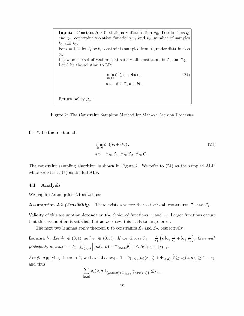
Input: Constant S > 0, stationary distribution µ0, distributions q1and q2, constraint violation functions v1 and v2, number of samplesk1 and k2.For i = 1, 2, let Ii be ki constraints sampled from Li under distributionqi.Let I be the set of vectors that satisfy all constraints in I1 and I2.Let θ be the solution to LP:

minθ∈Θ

ℓ⊤(µ0 +Φθ) , (24)

s.t. θ ∈ I, θ ∈ Θ .

Return policy µθ.

Figure 2: The Constraint Sampling Method for Markov Decision Processes

Let θ∗ be the solution of

minθ∈Θ

ℓ⊤(µ0 +Φθ) , (23)

s.t. θ ∈ L1, θ ∈ L2, θ ∈ Θ .

The constraint sampling algorithm is shown in Figure 2. We refer to (24) as the sampled ALP,

while we refer to (3) as the full ALP.

4.1 Analysis

We require Assumption A1 as well as:

Assumption A2 (Feasibility) There exists a vector that satisfies all constraints L1 and L2.

Validity of this assumption depends on the choice of functions v1 and v2. Larger functions ensure

that this assumption is satisfied, but as we show, this leads to larger error.

The next two lemmas apply theorem 6 to constraints L1 and L2, respectively.

Lemma 7. Let δ1 ∈ (0, 1) and ǫ1 ∈ (0, 1). If we choose k1 = 4ǫ1

(d log 12

ǫ1+ log 2

δ1

), then with

probability at least 1− δ1,∑

(x,a)

∣∣∣[µ0(x, a) + Φ(x,a),:θ]−

∣∣∣ ≤ SC1ǫ1 + ‖v1‖1.

Proof. Applying theorem 6, we have that w.p. 1 − δ1, q1(µ0(x, a) + Φ(x,a),:θ ≥ v1(x, a)) ≥ 1 − ǫ1,

and thus ∑

(x,a)

q1(x, a)I{µ0(x,a)+Φ(x,a),:θ<v1(x,a)}≤ ǫ1 .

19

Let L =∑

(x,a)

∣∣∣[µ0(x, a) + Φ(x,a),:θ]−

∣∣∣. With probability 1− δ1,

L =∑

(x,a)

∣∣∣[µ0(x, a) + Φ(x,a),:θ]−

∣∣∣ I{µ0(x,a)+Φ(x,a),:θ≤v1(x,a)}

+∑

(x,a)

∣∣∣[µ0(x, a) + Φ(x,a),:θ]−

∣∣∣ I{µ0(x,a)+Φ(x,a),:θ>v1(x,a)}

≤∑

(x,a)

∣∣∣Φ(x,a),:θ∣∣∣ I{µ0(x,a)+Φ(x,a),:θ≤v1(x,a)}

+ ‖v1‖1

≤∑

(x,a)

∥∥Φ(x,a),:

∥∥∥∥∥θ∥∥∥ I{µ0(x,a)+Φ(x,a),:θ≤v1(x,a)}

+ ‖v1‖1

≤∑

(x,a)

SC1q1(x, a)I{µ0(x,a)+Φ(x,a),:θ≤v1(x,a)}+ ‖v1‖1

≤ SC1ǫ1 + ‖v1‖1 .

Lemma 8. Let δ2 ∈ (0, 1) and ǫ2 ∈ (0, 1). If we choose k2 = 4ǫ2

(d log 12

ǫ2+ log 2

δ2

), then with

probability at least 1− δ2,∥∥∥(P −B)⊤Φθ

∥∥∥1≤ SC2ǫ2 + ‖v2‖1.

Proof. Applying theorem 6, we have that q2

(∣∣∣(P −B)⊤:,xΦθ∣∣∣ ≤ v2(x)

)≥ 1− ǫ2. This yields

∑

x

q2(x)I{|(P−B)⊤:,xΦθ|≥v2(x)}≤ ǫ2 . (25)

Let L′ =∑

x

∣∣∣(P −B)⊤:,xΦθ∣∣∣. Thus, with probability 1− δ2,

L′ =∑

x

∣∣∣(P −B)⊤:,xΦθ∣∣∣ I{|(P−B)⊤:,xΦθ|>v2(x)}

+∑

x

∣∣∣(P −B)⊤:,xΦθ∣∣∣ I{|(P−B)⊤:,xΦθ|≤v2(x)}

≤∑

x

∥∥∥(P −B)⊤:,xΦ∥∥∥∥∥∥θ∥∥∥ I{|(P−B)⊤:,xΦθ|>v2(x)}

+ ‖v2‖1

≤∑

x

SC2q2(x)I{|(P−B)⊤:,xΦθ|>v2(x)}+ ‖v2‖1

≤ SC2ǫ2 + ‖v2‖1 ,

where the last step follows from (25).

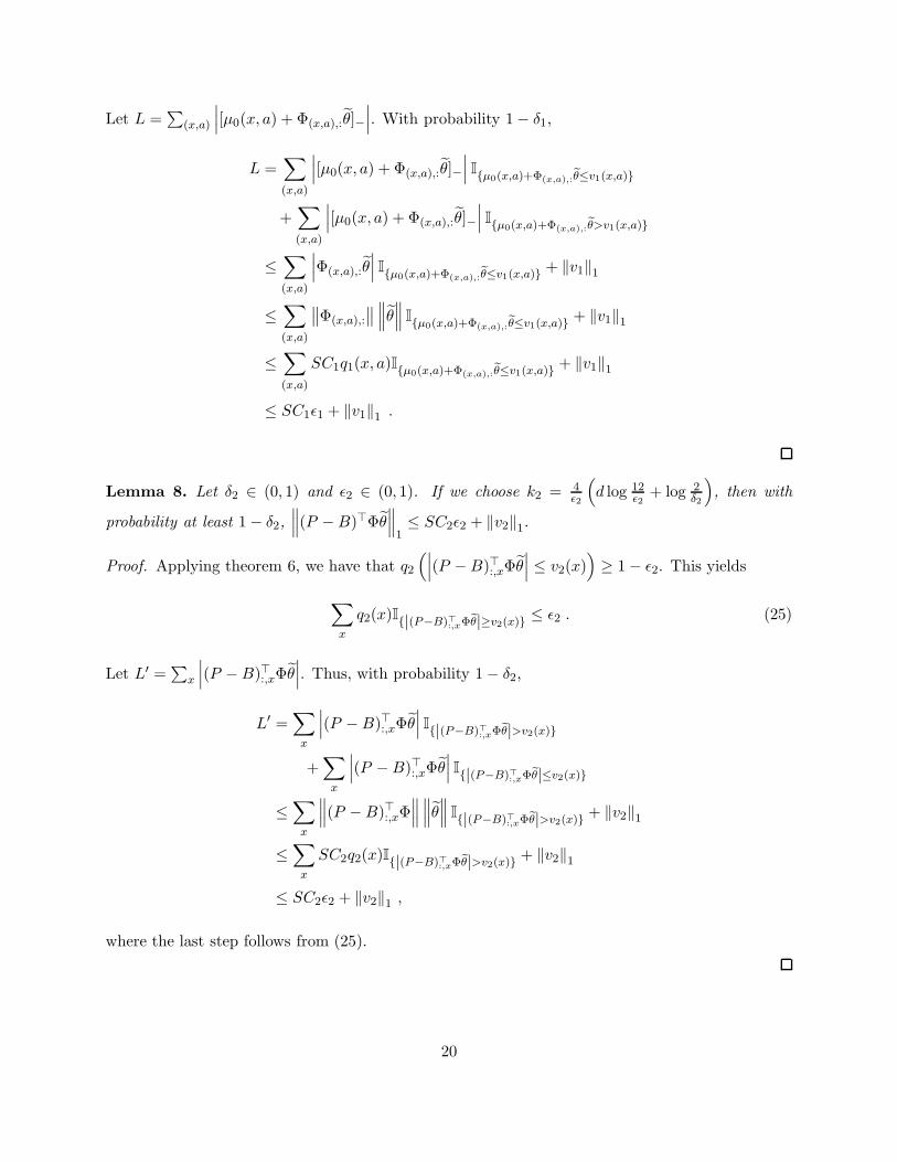
20

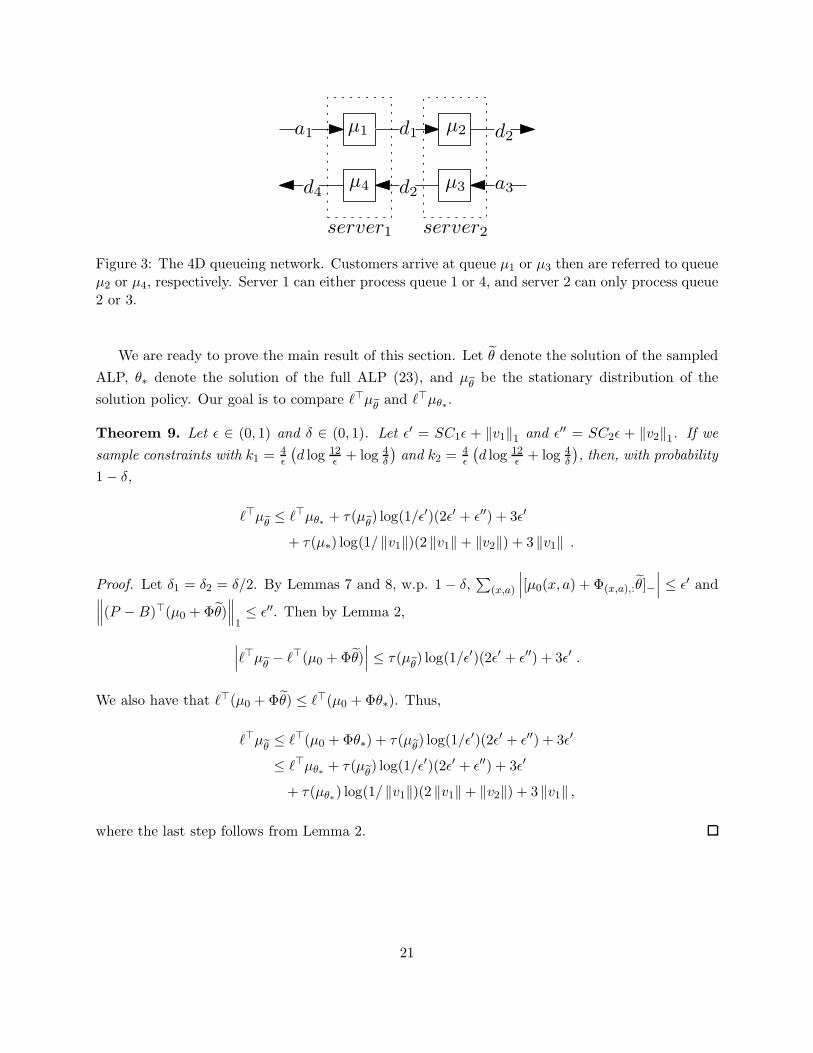
µ1 µ2

µ3µ4

d1a1

d2 a3

d2

d4

server1 server2

Figure 3: The 4D queueing network. Customers arrive at queue µ1 or µ3 then are referred to queueµ2 or µ4, respectively. Server 1 can either process queue 1 or 4, and server 2 can only process queue2 or 3.

We are ready to prove the main result of this section. Let θ denote the solution of the sampled

ALP, θ∗ denote the solution of the full ALP (23), and µθbe the stationary distribution of the

solution policy. Our goal is to compare ℓ⊤µθand ℓ⊤µθ∗.

Theorem 9. Let ǫ ∈ (0, 1) and δ ∈ (0, 1). Let ǫ′ = SC1ǫ + ‖v1‖1 and ǫ′′ = SC2ǫ + ‖v2‖1. If we

sample constraints with k1 =4ǫ

(d log 12

ǫ + log 4δ

)and k2 =

4ǫ

(d log 12

ǫ + log 4δ

), then, with probability

1− δ,

ℓ⊤µθ≤ ℓ⊤µθ∗ + τ(µ

θ) log(1/ǫ′)(2ǫ′ + ǫ′′) + 3ǫ′

+ τ(µ∗) log(1/ ‖v1‖)(2 ‖v1‖+ ‖v2‖) + 3 ‖v1‖ .

Proof. Let δ1 = δ2 = δ/2. By Lemmas 7 and 8, w.p. 1− δ,∑

(x,a)

∣∣∣[µ0(x, a) + Φ(x,a),:θ]−

∣∣∣ ≤ ǫ′ and∥∥∥(P −B)⊤(µ0 +Φθ)∥∥∥1≤ ǫ′′. Then by Lemma 2,

∣∣∣ℓ⊤µθ − ℓ⊤(µ0 +Φθ)∣∣∣ ≤ τ(µ

θ) log(1/ǫ′)(2ǫ′ + ǫ′′) + 3ǫ′ .

We also have that ℓ⊤(µ0 +Φθ) ≤ ℓ⊤(µ0 +Φθ∗). Thus,

ℓ⊤µθ≤ ℓ⊤(µ0 +Φθ∗) + τ(µ

θ) log(1/ǫ′)(2ǫ′ + ǫ′′) + 3ǫ′

≤ ℓ⊤µθ∗ + τ(µθ) log(1/ǫ′)(2ǫ′ + ǫ′′) + 3ǫ′

+ τ(µθ∗) log(1/ ‖v1‖)(2 ‖v1‖+ ‖v2‖) + 3 ‖v1‖ ,

where the last step follows from Lemma 2.

21

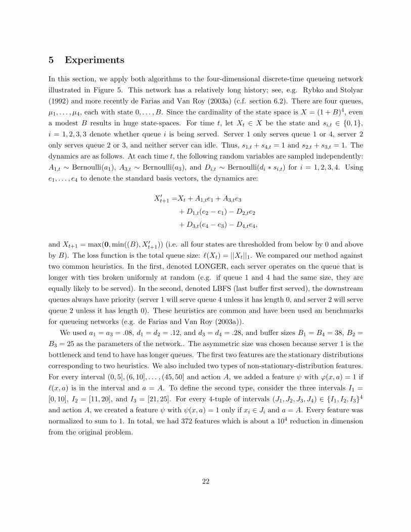
5 Experiments

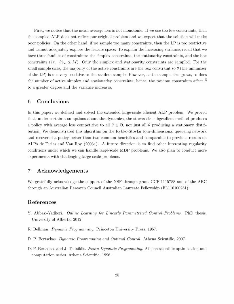
In this section, we apply both algorithms to the four-dimensional discrete-time queueing network

illustrated in Figure 5. This network has a relatively long history; see, e.g. Rybko and Stolyar

(1992) and more recently de Farias and Van Roy (2003a) (c.f. section 6.2). There are four queues,

µ1, . . . , µ4, each with state 0, . . . , B. Since the cardinality of the state space is X = (1 +B)4, even

a modest B results in huge state-spaces. For time t, let Xt ∈ X be the state and si,t ∈ {0, 1},i = 1, 2, 3, 3 denote whether queue i is being served. Server 1 only serves queue 1 or 4, server 2

only serves queue 2 or 3, and neither server can idle. Thus, s1,t + s4,t = 1 and s2,t + s3,t = 1. The

dynamics are as follows. At each time t, the following random variables are sampled independently:

A1,t ∼ Bernoulli(a1), A3,t ∼ Bernoulli(a3), and Di,t ∼ Bernoulli(di ∗ si,t) for i = 1, 2, 3, 4. Using

e1, . . . , e4 to denote the standard basis vectors, the dynamics are:

X ′t+1 =Xt +A1,te1 +A3,te3

+D1,t(e2 − e1)−D2,te2

+D3,t(e4 − e3)−D4,te4,

and Xt+1 = max(0,min((B),X ′t+1)) (i.e. all four states are thresholded from below by 0 and above

by B). The loss function is the total queue size: ℓ(Xt) = ||Xt||1. We compared our method against

two common heuristics. In the first, denoted LONGER, each server operates on the queue that is

longer with ties broken uniformly at random (e.g. if queue 1 and 4 had the same size, they are

equally likely to be served). In the second, denoted LBFS (last buffer first served), the downstream

queues always have priority (server 1 will serve queue 4 unless it has length 0, and server 2 will serve

queue 2 unless it has length 0). These heuristics are common and have been used an benchmarks

for queueing networks (e.g. de Farias and Van Roy (2003a)).

We used a1 = a3 = .08, d1 = d2 = .12, and d3 = d4 = .28, and buffer sizes B1 = B4 = 38, B2 =

B3 = 25 as the parameters of the network.. The asymmetric size was chosen because server 1 is the

bottleneck and tend to have has longer queues. The first two features are the stationary distributions

corresponding to two heuristics. We also included two types of non-stationary-distribution features.

For every interval (0, 5], (6, 10], . . . , (45, 50] and action A, we added a feature ψ with ϕ(x, a) = 1 if

ℓ(x, a) is in the interval and a = A. To define the second type, consider the three intervals I1 =

[0, 10], I2 = [11, 20], and I3 = [21, 25]. For every 4-tuple of intervals (J1, J2, J3, J4) ∈ {I1, I2, I3}4and action A, we created a feature ψ with ψ(x, a) = 1 only if xi ∈ Ji and a = A. Every feature was

normalized to sum to 1. In total, we had 372 features which is about a 104 reduction in dimension

from the original problem.

22

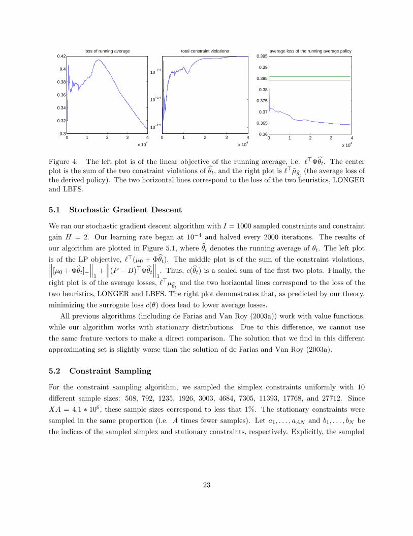
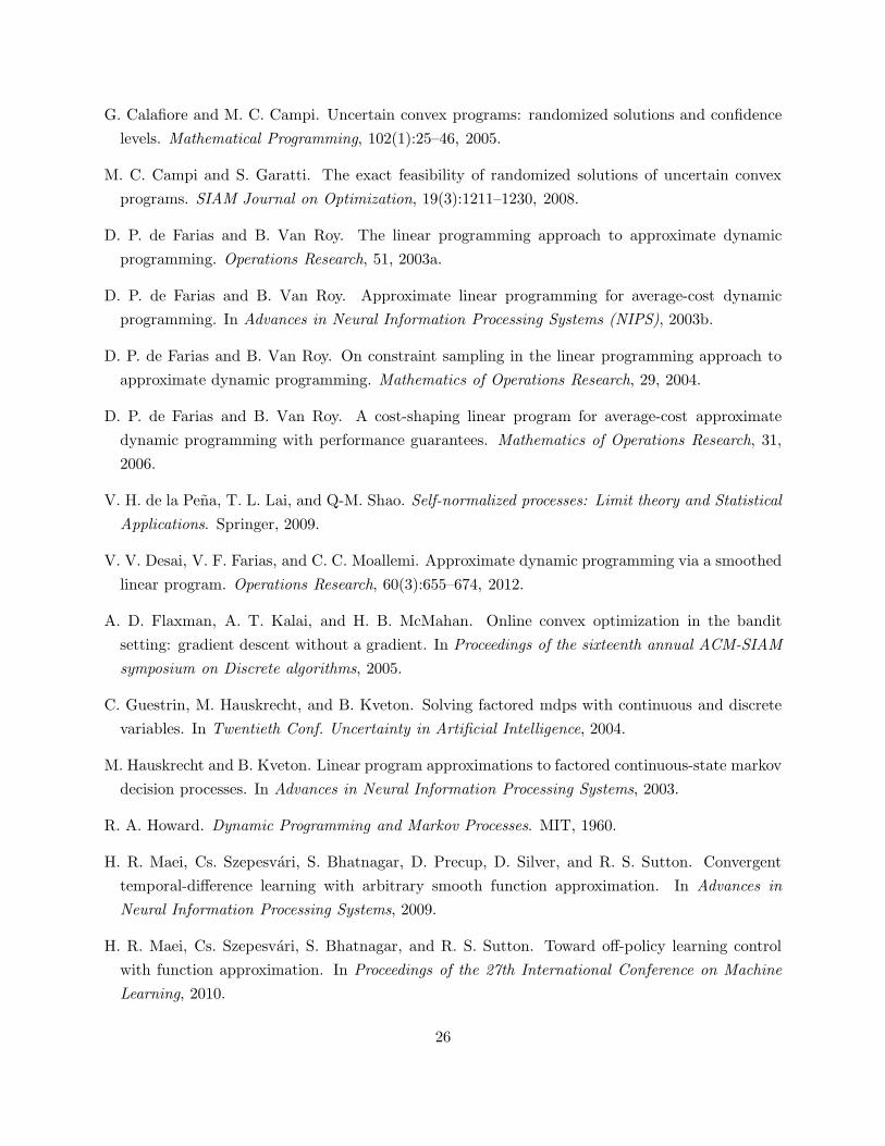
0 1 2 3 4

x 104

0.3

0.32

0.34

0.36

0.38

0.4

0.42loss of running average

0 1 2 3 4

x 104

10−2.5

10−2.4

10−2.3

total constraint violations

0 1 2 3 4

x 104

0.36

0.365

0.37

0.375

0.38

0.385

0.39

0.395average loss of the running average policy

Figure 4: The left plot is of the linear objective of the running average, i.e. ℓ⊤Φθt. The centerplot is the sum of the two constraint violations of θt, and the right plot is ℓ⊤µ

θt(the average loss of

the derived policy). The two horizontal lines correspond to the loss of the two heuristics, LONGERand LBFS.

5.1 Stochastic Gradient Descent

We ran our stochastic gradient descent algorithm with I = 1000 sampled constraints and constraint

gain H = 2. Our learning rate began at 10−4 and halved every 2000 iterations. The results of

our algorithm are plotted in Figure 5.1, where θt denotes the running average of θt. The left plot

is of the LP objective, ℓ⊤(µ0 + Φθt). The middle plot is of the sum of the constraint violations,∥∥∥[µ0 +Φθt]−

∥∥∥1+∥∥∥(P −B)⊤Φθt

∥∥∥1. Thus, c(θt) is a scaled sum of the first two plots. Finally, the

right plot is of the average losses, ℓ⊤µθt

and the two horizontal lines correspond to the loss of the

two heuristics, LONGER and LBFS. The right plot demonstrates that, as predicted by our theory,

minimizing the surrogate loss c(θ) does lead to lower average losses.

All previous algorithms (including de Farias and Van Roy (2003a)) work with value functions,

while our algorithm works with stationary distributions. Due to this difference, we cannot use

the same feature vectors to make a direct comparison. The solution that we find in this different

approximating set is slightly worse than the solution of de Farias and Van Roy (2003a).

5.2 Constraint Sampling

For the constraint sampling algorithm, we sampled the simplex constraints uniformly with 10

different sample sizes: 508, 792, 1235, 1926, 3003, 4684, 7305, 11393, 17768, and 27712. Since

XA = 4.1 ∗ 106, these sample sizes correspond to less that 1%. The stationary constraints were

sampled in the same proportion (i.e. A times fewer samples). Let a1, . . . , aAN and b1, . . . , bN be

the indices of the sampled simplex and stationary constraints, respectively. Explicitly, the sampled

23

LP is:

minθ

(Φθ)⊤ℓ , (26)

s.t. (Φθ)⊤1 = 1, Φai,;θ ≥ 0, ∀i = 1, . . . , AN,∣∣∣Φθ⊤(P −B):,bi

∣∣∣ ≤ ǫs, ∀i = 1, . . . , N, ‖θ‖∞ ≤M (27)

where M and ǫ are necessary to ensure the LP always has a feasible and bounded solution. This

corresponds to setting v1 = 0 and v2 = ǫ. In particular, we used M = 3 and ǫ = 10−3. Using

differenc values of ǫ did not have a large effect on the behavior of the algorithm.

For each sample size, we sample the constraints, solve the LP, then simulate the average loss of

the policy. We repeated this procedure 35 times for each sample size and plotted the mean with

error bars corresponding to the variance across each sample size in Figure 5.2. Note the log scale

on the x-axis. The best loss corresponds to 4684 sampled simplex constraints, or roughly 1%, and

is a marked improvement over the average loss found by the stochastic gradient descent method.

However, changing the sample size by a factor of 4 in either direction is enough to obliterate this

advantage.

103

104

25

30

35

40

45

50

55

60

65

70

number of simplex constraints sampled

aver

age

loss

average loss produced by the constraint sampling algorithm with variance bars

Figure 5: Average loss with variance error bars of the constraint sampling algorithm run with avariety of sample sizes.

24

First, we notice that the mean average loss is not monotonic. If we use too few constraints, then

the sampled ALP does not reflect our original problem and we expect that the solution will make

poor policies. On the other hand, if we sample too many constraints, then the LP is too restrictive

and cannot adequately explore the feature space. To explain the increasing variance, recall that we

have three families of constraints: the simplex constraints, the stationarity constraints, and the box

constraints (i.e. |θ|∞ ≤ M). Only the simplex and stationarity constraints are sampled. For the

small sample sizes, the majority of the active constraints are the box constraint so θ (the minimizer

of the LP) is not very sensitive to the random sample. However, as the sample size grows, so does

the number of active simplex and stationarity constraints; hence, the random constraints affect θ

to a greater degree and the variance increases.

6 Conclusions

In this paper, we defined and solved the extended large-scale efficient ALP problem. We proved

that, under certain assumptions about the dynamics, the stochastic subgradient method produces

a policy with average loss competitive to all θ ∈ Θ, not just all θ producing a stationary distri-

bution. We demonstrated this algorithm on the Rybko-Stoylar four-dimensional queueing network

and recovered a policy better than two common heuristics and comparable to previous results on

ALPs de Farias and Van Roy (2003a). A future direction is to find other interesting regularity

conditions under which we can handle large-scale MDP problems. We also plan to conduct more

experiments with challenging large-scale problems.

7 Acknowledgements

We gratefully acknowledge the support of the NSF through grant CCF-1115788 and of the ARC

through an Australian Research Council Australian Laureate Fellowship (FL110100281).

References

Y. Abbasi-Yadkori. Online Learning for Linearly Parametrized Control Problems. PhD thesis,

University of Alberta, 2012.

R. Bellman. Dynamic Programming. Princeton University Press, 1957.

D. P. Bertsekas. Dynamic Programming and Optimal Control. Athena Scientific, 2007.

D. P. Bertsekas and J. Tsitsiklis. Neuro-Dynamic Programming. Athena scientific optimization and

computation series. Athena Scientific, 1996.

25

G. Calafiore and M. C. Campi. Uncertain convex programs: randomized solutions and confidence

levels. Mathematical Programming, 102(1):25–46, 2005.

M. C. Campi and S. Garatti. The exact feasibility of randomized solutions of uncertain convex

programs. SIAM Journal on Optimization, 19(3):1211–1230, 2008.

D. P. de Farias and B. Van Roy. The linear programming approach to approximate dynamic

programming. Operations Research, 51, 2003a.

D. P. de Farias and B. Van Roy. Approximate linear programming for average-cost dynamic

programming. In Advances in Neural Information Processing Systems (NIPS), 2003b.

D. P. de Farias and B. Van Roy. On constraint sampling in the linear programming approach to

approximate dynamic programming. Mathematics of Operations Research, 29, 2004.

D. P. de Farias and B. Van Roy. A cost-shaping linear program for average-cost approximate

dynamic programming with performance guarantees. Mathematics of Operations Research, 31,

2006.

V. H. de la Pena, T. L. Lai, and Q-M. Shao. Self-normalized processes: Limit theory and Statistical

Applications. Springer, 2009.

V. V. Desai, V. F. Farias, and C. C. Moallemi. Approximate dynamic programming via a smoothed

linear program. Operations Research, 60(3):655–674, 2012.

A. D. Flaxman, A. T. Kalai, and H. B. McMahan. Online convex optimization in the bandit

setting: gradient descent without a gradient. In Proceedings of the sixteenth annual ACM-SIAM

symposium on Discrete algorithms, 2005.

C. Guestrin, M. Hauskrecht, and B. Kveton. Solving factored mdps with continuous and discrete

variables. In Twentieth Conf. Uncertainty in Artificial Intelligence, 2004.

M. Hauskrecht and B. Kveton. Linear program approximations to factored continuous-state markov

decision processes. In Advances in Neural Information Processing Systems, 2003.

R. A. Howard. Dynamic Programming and Markov Processes. MIT, 1960.

H. R. Maei, Cs. Szepesvari, S. Bhatnagar, D. Precup, D. Silver, and R. S. Sutton. Convergent

temporal-difference learning with arbitrary smooth function approximation. In Advances in

Neural Information Processing Systems, 2009.

H. R. Maei, Cs. Szepesvari, S. Bhatnagar, and R. S. Sutton. Toward off-policy learning control

with function approximation. In Proceedings of the 27th International Conference on Machine

Learning, 2010.

26

A. S. Manne. Linear programming and sequential decisions. Management Science, 6(3):259–267,

1960.

M. Petrik and S. Zilberstein. Constraint relaxation in approximate linear programs. In Proc. 26th

Internat. Conf. Machine Learning (ICML), 2009.

A. N. Rybko and A. L. Stolyar. Ergodicity of stochastic processes describing the operation of open

queueing networks. Problemy Peredachi Informatsii, 28(3):3–26, 1992.

P. Schweitzer and A. Seidmann. Generalized polynomial approximations in Markovian decision

processes. Journal of Mathematical Analysis and Applications, 110:568–582, 1985.

R. S. Sutton and A. G. Barto. Reinforcement Learning: An Introduction. Bradford Book. MIT

Press, 1998.

R. S. Sutton, H. R. Maei, D. Precup, S. Bhatnagar, D. Silver, Cs. Szepesvari, and E. Wiewiora. Fast

gradient-descent methods for temporal-difference learning with linear function approximation. In

Proceedings of the 26th International Conference on Machine Learning, 2009a.

R. S. Sutton, Cs. Szepesvari, and H. R. Maei. A convergent O(n) algorithm for off-policy temporal-

difference learning with linear function approximation. In Advances in Neural Information Pro-

cessing Systems, 2009b.

M. H. Veatch. Approximate linear programming for average cost mdps. Mathematics of Operations

Research, 38(3), 2013.

T. Wang, D. Lizotte, M. Bowling, and D. Schuurmans. Dual representations for dynamic program-

ming. Journal of Machine Learning Research, pages 1–29, 2008.

M. Zinkevich. Online convex programming and generalized infinitesimal gradient ascent. In ICML,

2003.

27