1

SNR walls for signal detection

Rahul Tandra Anant Sahai

tandra@eecs.berkeley.edu sahai@eecs.berkeley.edu

Dept. of Electrical Engineering and Computer Sciences, U C Berkeley

Abstract

This paper considers the detection of the presence/absenceof signals in uncertain low SNR environments.

Small modeling uncertainties are unavoidable in any practical system and so robustness to them is a fundamentally

important performance metric. The impact of these modelinguncertainties can be quantified by the position of the

“SNR wall” below which any particular detector will fail to be robust, no matter how long it can observe the channel.

We propose simple mathematical models for the uncertainty in the noise distribution and the fading process and

show what aspects of the model lead to SNR walls for differinglevels of knowledge of the signal to be detected.

These results have implications for wireless spectrum regulators. The context is opportunistically sharing spec-

trum with primary users that must be detected in order to avoid causing harmful interference on a channel. Ideally,

a secondary system would be able to detect primaries robustly without having to know much about their signaling

strategies. We argue that the tension between primary and secondary users is captured by the technical question of

computing the optimal tradeoff betweencapacityand robustnessas quantified by the SNR wall. This is an open

problem, but we compute this tradeoff for some simple detectors.

I. I NTRODUCTION

In order to recycle underutilized spectrum, the operation of unlicensed secondary devices within licensed primary

bands such as “unused” television broadcast bands has been proposed [1]. The main constraint for opportunistic

secondary devices/cognitive radios is guaranteeing non-interference to the primary system. One possibility is to

dynamically align the secondary transmissions such that the resulting interference is mostly orthogonal to the

primary’s received signal [2] or by having the secondary user counteract its own interference in the direction of

the primary signals [3]. Such design strategies face severalpractical problems. The two systems must be jointly

engineered and may require a huge overhead in terms of the amount of coordination between the primary and

secondary systems. Furthermore, even simple phase uncertainties can significantly lower the performance of such

collaborative designs [4].

Another possible strategy is for the secondary user to sensefor primary signals and opportunistically use a primary

channel only if sensing declares the channel to be vacant. This approach has the advantage of minimal coordination

2

with primary systems and hence is more flexible, but this flexibility comes at the cost of lower performance when

many primaries are present. The opportunistic approach is also fair in the sense that the onus is on the secondary

system to sense for the primary if it wants to use the spectrum. However, in order to guarantee non-interference

with potentially hidden primary receivers, the secondary system needs to be able to detect the presence/absence of

very weak primary signals [5], [6]. The IEEE 802.22 is the first international standards process for a cognitive-radio

based PHY/MAC/air interface for use in spectrum that is allocated to Television as the primary user. Under the

currently understood requirements, secondary devices arerequired to sense TV transmissions as low as−116 dBm

(SNR = −22 dB) [7], [8].

In spectrum sensing, the goal is to meet a given ‘receiver operating characteristic’ (ROC) constraint at very

low SNR. Classical detection theory suggests that degradation in the ROC due to reduced SNR can be countered

by increasing the sensing time [9], [10]. Hence, the sensitivity is considered to be limited by higher layer design

considerations. For instance, the QoS requirements of the application drive the protocol layer design, which in turn

dictates the time available for sensing by the physical layer. This traditional perspective implies that a cognitive

radio system can always be engineered at the cost of low enough QoS.

In a real-world physical system, parameters are never knownto infinite precision. To list just a few, real-world

background “noise” is not perfectly Gaussian, it is not perfectly white, nor is it perfectly stationary. The channel

fading is neither flat nor is it constant over time. Real-worldfilters are not ideal, A/D converters have finite precision

and dynamic range,I and Q signal pathways in a receiver are never perfectly matched and local oscillators are

never perfect sine-waves. This paper argues that as a result of these uncertainties, the degradation in QoS may be

complete once the target primary SNR is low enough.These model uncertainties impose fundamental limitations

on detection performance. The limitations cannot be countered by increasing the sensing duration. At very low

SNRs, the ergodic view of the world is no longer valid, i.e., one cannot count on infinite averaging to combat the

relevant uncertainties.

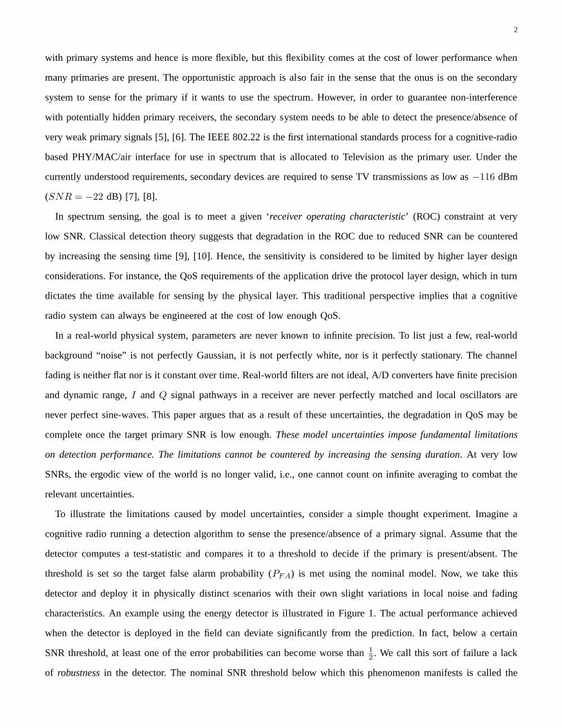
To illustrate the limitations caused by model uncertainties, consider a simple thought experiment. Imagine a

cognitive radio running a detection algorithm to sense the presence/absence of a primary signal. Assume that the

detector computes a test-statistic and compares it to a threshold to decide if the primary is present/absent. The

threshold is set so the target false alarm probability (PFA) is met using the nominal model. Now, we take this

detector and deploy it in physically distinct scenarios with their own slight variations in local noise and fading

characteristics. An example using the energy detector is illustrated in Figure 1. The actual performance achieved

when the detector is deployed in the field can deviate significantly from the prediction. In fact, below a certain

SNR threshold, at least one of the error probabilities can become worse than12 . We call this sort of failure a lack

of robustnessin the detector. The nominal SNR threshold below which this phenomenon manifests is called the

3

SNR wallfor the detector.

0 0.05 0.1 0.15 0.2 0.25 0.3 0.35 0.4 0.45 0.50

0.05

0.1

0.15

0.2

0.25

0.3

0.35

0.4

0.45

0.5ROC curves for energy detection (N=2000, SNR = −10 dB, x=.25)

Probability of false alarm PFA

Pro

babi

lity

of m

is−d

etec

tion

PM

DTargetPerformance

Fig. 1. Error probabilities of energy detection under noise uncertainty. The point marked by an ‘X ’ is the target theoretical performanceunder a nominal SNR of−10. The shaded area illustrates the range of performance achieved with actual SNR’s varying between−9.9 dBand−10.1 dB (x = .1 in Sec III-A2).

Such robustness limits were first shown in the context of radiometric (energy) detection of spread spectrum

signals [11]. To make progress for general classes of signals and detection algorithms, it is important to distill the

relevant uncertainties into tractable mathematical models that enable us to focus on the uncertainties that are most

critical. The basic sensing problem is posed in Section II withthe explicit models for practical wireless system

uncertainties in noise and fading being introduced gradually throughout this paper. Section III then explores the

robustness of two extreme cases — non-coherent detectors and pilot-detection. The former corresponds to very

limited knowledge about the primary signaling scheme whereas the latter corresponds to complete knowledge of

a part of the primary’s signal. Both of these detectors suffer from SNR walls. In particular, the best possible

non-coherent detector is essentially as non-robust as the energy detector and this non-robustness arises from the

distributional uncertainty in the background noise. In thecoherent case, the SNR wall is pushed back, but only to

an extent limited by the finite coherence time of the fading process. It is important to note that these SNR walls

are not modeling artifacts. They have been experimentally verified in [12] using controlled experiments that were

carefully calibrated to limit uncertainties.

Once it is clear that uncertainties limit detector performance, it is natural to consider detection strategies that

attempt to learn the characteristics of the environment at run-time and thereby reduce the uncertainty. We call

this approachnoise calibrationand it is explored in Section IV. First, pilot detection is revisited. The key idea is

that the pilot tone does not fill all degrees of freedom at the receiver and so the other degrees of freedom can be

used to learn the noise model. Such strategies can improve performance only so far, with the limit coming from

a combination of the non-whiteness of the background noise process and the finite coherence-time of the fading

4

process. Frequency is not the only way to think about degrees of freedom. So next, noise calibration is explored in

time domain by considering primary signals whose pulses have only a 50% duty cycle. In this example, the limits

to noise calibration are due to the uncertain frequency selectivity of the fading and the concept ofdelay coherence

time is introduced to capture this.

The robustness results in this paper have significant implications for policymakers. Suppose that a band of

spectrum is opened for cognitive use. The rules governing theband must be flexible enough to allow interoperability

with future technologies while also being compatible with high performance. One can think of a simple and flexible

rule: the primary can transmit any signal within a given spectral mask, similarly the secondary should be able to

robustly sense the primary with a high probability of detection. Under these rules, the primary could potentially

use all its degrees of freedom by transmitting a ‘white’ signal. As shown in Section III-A, the secondary would

be forced to non-coherently detect for the primary, and suchdetection algorithms are highly non-robust. Complete

flexibility for the primary user comes at a cost of inefficient spectral usage overall. The secondary systems face

SNR walls and hence are forced to presumptively shut-up sincethey cannot robustly detect the absence of potential

primary signals. But, if the rules are written so that the primary is mandated to transmit a known pilot tone at a

certain power, then the secondary systems can operate more easily at the cost of potentially lower performance

for the primary user. The general tradeoff can be posed technically as thecapacity-robustness tradeoff. We briefly

discuss this tradeoff in Section V for some of the detectors considered here.

II. PROBLEM FORMULATION

Let X(t) denote the band-limited signal we are trying to sense, letH denote the fading process, and let the

additive noise process beW (t). Although this paper focuses on real-valued signals, the analysis easily extends to

complex signals. The discrete-time version is obtained by sampling the received signal at the appropriate rate. The

sensing problem can be formulated as a binary hypothesis testing problem with the following hypotheses:

H0 : Y [n] = W [n]

H1 : Y [n] = HX[n] + W [n] (1)

Here X[n] are the samples of the signal of interest,H is a linear time-varying operator,W [n] are samples of

noise andY [n] are the received signal samples. Throughout this paper, thesignal is assumed to be independent

of both the noise and the fading process. Random processes are also assumed to be stationary and ergodic unless

otherwise specified.

All three aspects of the system(W, H, X) admit statistical models, but it is unrealistic to assume complete

knowledge of their parameters to infinite precision. To understand the issue of robustness to uncertainty, we assume

5

knowledge of their distributions within some bounds and areinterested in the worst case performance of detection

algorithms over the uncertain distributions.1

Background noise is an aggregation of various sources like thermal noise, leakage of signals from other bands due

to receiver non-linearity, aliasing from imperfect front end filters, interference due to transmissions from licensed

users far away, interference from other opportunistic systems in the vicinity, etc. A stationary white Gaussian

assumption is only an approximation2 and so the noise samplesW [n] are modeled as having any distributionW

from a set of possible distributionsWx. This set is called the noise uncertainty set and specific models for it

are considered in subsequent sections. The goal is to introduce only as much uncertainty as needed to show that

detection becomes non-robust.

Fading is modeled with the same philosophy. The fading process H ∈ Hf is considered a linear time varying

filter and models for it will be developed as needed. The generalidea is that filter coefficients vary on the time-scale

given by the channel coherence time, but it is unreasonable to assume that the true channel coherence time is known

exactly. All we can hope for are bounds on it.

Finally, uncertainty arises due tointentional under-modelingof system parameters. For instance, the primary

signalX can be modeled by imposing a cap on its power spectral density, instead of actually modeling its specific

signal constellation, waveform, etc. The advantage of under-modeling is two-fold. Firstly, it leads to less complex

systems. Secondly, intentional under-modeling keeps the model flexible. For example, a simple power spectral

density cap on a chunk of spectrum is advantageous because itgives the primary user flexibility to choose from a

diverse set of signaling strategies. This is useful for ease of system evolution.

Any detection strategy/algorithm can be written as a possibly random functionF : RN → {0, 1}, whereF maps

theN dimensional received vectorY = (Y [1], Y [2], · · · , Y [N ]) onto the set{0, 1}. Here ‘0’ stands for the decision

that the received signal is noise and ‘1’ stands for the decision that the received signal is signal plus noise. For

each choice of a noise distributionW ∈ Wx and fading modelH ∈ Hf , the error probabilities are

PFA(W, H) = EW,H

[1{F=1}|H0

]; PMD(W, H) = EW,H

[1{F=0}|H1

].

• A decision strategyrobustlyachieves a given target probability of false alarm,PFA, and probability of missed

detection,PMD if the algorithm satisfies

supW∈Wx,H∈Hf

PFA(W, H) ≤ PFA; supW∈Wx,H∈Hf

PMD(W, H) ≤ PMD.

1If a Bayesian perspective is taken and a prior is assumed over these parameters, then nothing much changes. The prior turns into a setof possible parameter values once a desired probability of missed detection and false alarm are set. Having a prior just makes the notationand definitions more complicated and so we do not assume priors here for system parameters.

2In information theory, it turns out that the Gaussian distribution is a saddle point for many interesting optimization problems. Therefore,we are sometimes safe in ignoring the distributional uncertainty and just overbounding with a worst case Gaussian. However, this turns outnot to be true in our case.

6

• The average signal to noise ratio is defined as

SNR =P

σ2n

, whereP = limN→∞

1

N

N∑

n=1

X[n]2.

Although the actual noise variance might vary over distributions in the setWx, we assume that there is a

single nominal noise varianceσ2n associated with the noise uncertainty setWx.

• A detection algorithm isnon-robust at a fixed SNR if the algorithm cannot robustly achieve any pair

(PFA, PMD), where0 ≤ PFA < 12 and0 ≤ PMD < 1

2 , irrespective of the sampling durationN .

• Suppose there exists a signal to noise ratio threshold,SNRt, such that the detector is non-robust for all

SNR ≤ SNRt. The maximum value of such a threshold is defined as theSNR wall for the detector.

SNRwall = sup{SNRt, s.t., the detector is non-robust for allSNR ≤ SNRt}.

An equivalent condition for testing robustness of a detector can be given in terms of the test statisticT (Y)

for the detector. The detector is non-robust iff the sets of means ofT (Y) under both hypotheses overlap [13],

[14]. Mathematically, for a fixedN , define AN := {EW,H [T (Y)|H0] : W ∈ Wx, H ∈ Hf} and BN :=

{EW,H [T (Y)|H1] : W ∈ Wx, H ∈ Hf}. The detector is non-robust iffAN ∩BN 6= ∅ for all N > 0. Furthermore,

if the set of distributions for the observationsY under both hypotheses overlap then every detection algorithm will

be non-robust. This criterion is used throughout this paper to verify if a given detection algorithm is non-robust.

The goal of this paper is to analyze detection algorithms and prove the existence ofSNR walls.

III. D ETECTOR ROBUSTNESS: TWO EXTREME CASES

A. Unknown signal structure

Consider a situation where the spectrum sensor knows very little about the primary signal. Assume that the

primary signaling scheme is unknown, except with a known power within the band of interest. This corresponds to

a primary licensee that has absolute freedom to choose its signaling strategy with only the bandwidth and power

specified in the license. To robustly detect such a primary user, a single detector must be able to detect the presence

of any possible primary signal that satisfies the power and bandwidth constraint.

Under this limited information, the intuitively hardest signal to detect is a zero-mean white signal in the frequency

band of interest.

1) Radiometer robustness:It is useful to review the radiometer (energy detector) under noise level uncertainty

[11]. The test statistic is given byT (Y) = 1N

∑Nn=1 Y [n]2. If there is no uncertainty and the noise variance is

completely known, the central limit theorem (see [15]) gives the following approximations:

T (Y)|H0 ∼ N (σ2,1

N2σ4), T (Y)|H1 ∼ N (P + σ2,

1

N2(P + σ2)2),

7

whereP is the average signal power andσ2 is the noise variance. Using these approximations gives

PFA = Prob (T (Y) > γ|H0)

= Q

γ − σ2

√2N σ2

, (2)

whereγ is the detector threshold. Similarly, the probability of detection is given by

PD = Q

γ − (P + σ2)√

2N (P + σ2)

(3)

Eliminating γ from (2) and (3), we getN = 2[Q−1(PFA)−Q−1(PD)(1 + SNR)]2SNR−2. At low SNR we can

approximate1 + SNR ≈ 1 and this gives a sample complexityN = O(SNR−2). This shows that if the noise

statistics are completely known, then we can detect signalsat arbitrarily lowSNR’s by increasing the sensing time

N .

Now, consider the case with uncertainty in the noise model. Since the radiometer only sees energy, the distribu-

tional uncertainty of noise can be summarized in a single interval [1ρσ2n, ρσ2

n] whereσ2n is the nominal noise power

andρ > 1 is a parameter that quantifies the size of the uncertainty.

To see the sample complexity required to achieve a targetPFA andPD robustly, (2) and (3) are modified to get

PFA = maxσ2∈[ 1

ρσ2

n,ρσ2n]Q

γ − σ2

√2N σ2

= Q

γ − ρσ2

n√2N ρσ2

n

,

PD = minσ2∈[ 1

ρσ2

n,ρσ2n]Q

γ − (P + σ2)√

2N (P + σ2)

= Q

γ − (P + 1

ρσ2n)

√2N (P + 1

ρσ2n)

. (4)

Approximating1 + SNR ≈ 1 gives

N =2[Q−1(PFA) −Q−1(PD)]2

[SNR −

(ρ − 1

ρ

)]2 . (5)

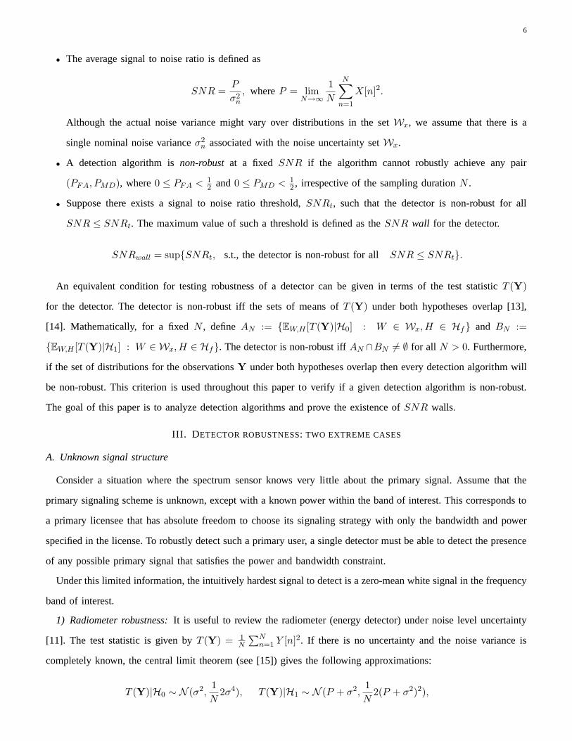
From the above expression it is clear thatN → ∞ as SNR ↓(ρ − 1

ρ

), and this is illustrated in Figure 2. The

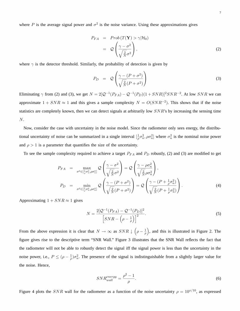
figure gives rise to the descriptive term “SNR Wall.” Figure 3 illustrates that the SNR Wall reflects the fact that

the radiometer will not be able to robustly detect the signaliff the signal power is less than the uncertainty in the

noise power, i.e.,P ≤ (ρ − 1ρ)σ2

n. The presence of the signal is indistinguishable from a slightly larger value for

the noise. Hence,

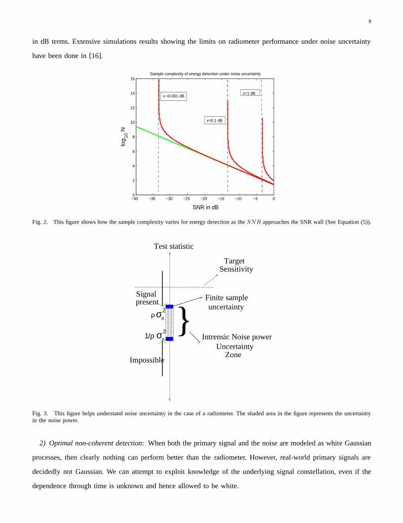
SNRenergywall =

ρ2 − 1

ρ. (6)

Figure 4 plots theSNR wall for the radiometer as a function of the noise uncertainty ρ = 10x/10, as expressed

8

in dB terms. Extensive simulations results showing the limits on radiometer performance under noise uncertainty

have been done in [16].

−40 −35 −30 −25 −20 −15 −10 −5 00

2

4

6

8

10

12

14

16

SNR in dB

log

10 N

Sample complexity of energy detection under noise uncertainty

x =0.001 dB

x=0.1 dB

x=1 dB

Fig. 2. This figure shows how the sample complexity varies for energy detection as theSNR approaches the SNR wall (See Equation (5)).

Signalpresent

TargetSensitivity

σ2n

σ2n

Finite sampleuncertainty

UncertaintyZone

Intrensic Noise power}

Impossible

Test statistic

1/ρ

ρ

Fig. 3. This figure helps understand noise uncertainty in the case of a radiometer. The shaded area in the figure represents the uncertaintyin the noise power.

2) Optimal non-coherent detection:When both the primary signal and the noise are modeled as white Gaussian

processes, then clearly nothing can perform better than theradiometer. However, real-world primary signals are

decidedly not Gaussian. We can attempt to exploit knowledgeof the underlying signal constellation, even if the

dependence through time is unknown and hence allowed to be white.

9

0 0.5 1 1.5 2 2.5 3−14

−12

−10

−8

−6

−4

−2

0

2Position of SNR wall for radiometer

Noise uncertainty x (in dB)

SN

Rw

all (

in d

B)

−3.3 dB

Fig. 4. This figure plots theSNRenergywall in (6) as a function of noise level uncertaintyx whereρ = 10x/10. The point marked by a “x”

on the plot corresponds to x=1 dB of device level noise uncertainty.

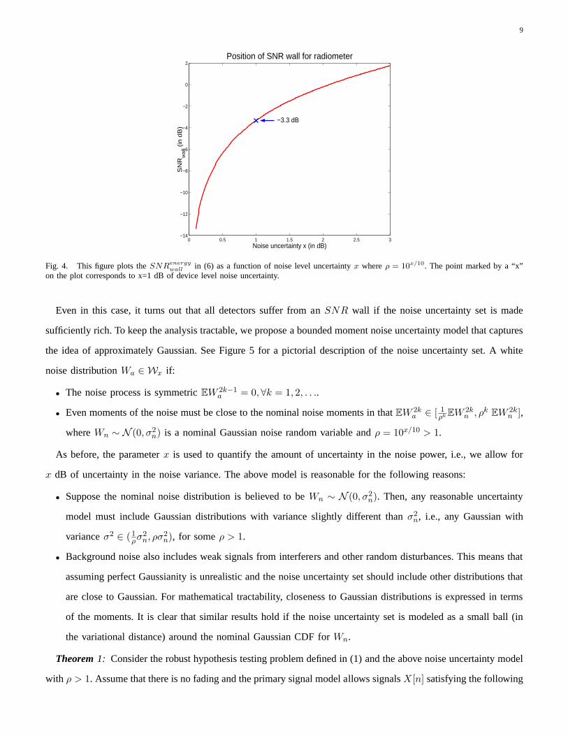
Even in this case, it turns out that all detectors suffer from an SNR wall if the noise uncertainty set is made

sufficiently rich. To keep the analysis tractable, we proposea bounded moment noise uncertainty model that captures

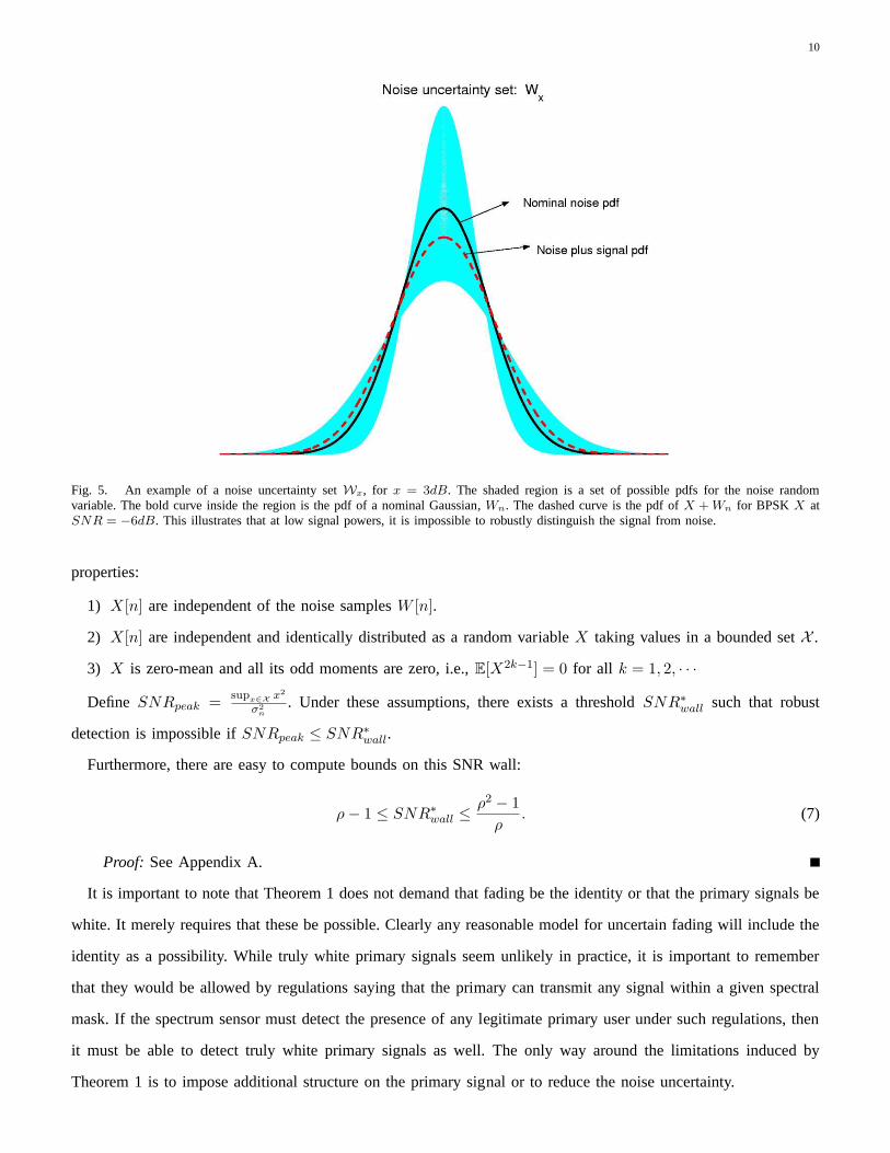
the idea of approximately Gaussian. See Figure 5 for a pictorial description of the noise uncertainty set. A white

noise distributionWa ∈ Wx if:

• The noise process is symmetricEW 2k−1a = 0,∀k = 1, 2, . . ..

• Even moments of the noise must be close to the nominal noise moments in thatEW 2ka ∈ [ 1

ρk EW 2kn , ρk EW 2k

n ],

whereWn ∼ N (0, σ2n) is a nominal Gaussian noise random variable andρ = 10x/10 > 1.

As before, the parameterx is used to quantify the amount of uncertainty in the noise power, i.e., we allow for

x dB of uncertainty in the noise variance. The above model is reasonable for the following reasons:

• Suppose the nominal noise distribution is believed to beWn ∼ N (0, σ2n). Then, any reasonable uncertainty

model must include Gaussian distributions with variance slightly different thanσ2n, i.e., any Gaussian with

varianceσ2 ∈ (1ρσ2

n, ρσ2n), for someρ > 1.

• Background noise also includes weak signals from interferers and other random disturbances. This means that

assuming perfect Gaussianity is unrealistic and the noise uncertainty set should include other distributions that

are close to Gaussian. For mathematical tractability, closeness to Gaussian distributions is expressed in terms

of the moments. It is clear that similar results hold if the noise uncertainty set is modeled as a small ball (in

the variational distance) around the nominal Gaussian CDF for Wn.

Theorem 1: Consider the robust hypothesis testing problem defined in (1)and the above noise uncertainty model

with ρ > 1. Assume that there is no fading and the primary signal model allows signalsX[n] satisfying the following

10

Fig. 5. An example of a noise uncertainty setWx, for x = 3dB. The shaded region is a set of possible pdfs for the noise randomvariable. The bold curve inside the region is the pdf of a nominal Gaussian, Wn. The dashed curve is the pdf ofX + Wn for BPSK X atSNR = −6dB. This illustrates that at low signal powers, it is impossible to robustly distinguish the signal from noise.

properties:

1) X[n] are independent of the noise samplesW [n].

2) X[n] are independent and identically distributed as a random variable X taking values in a bounded setX .

3) X is zero-mean and all its odd moments are zero, i.e.,E[X2k−1] = 0 for all k = 1, 2, · · ·

Define SNRpeak =supx∈X

x2

σ2n

. Under these assumptions, there exists a thresholdSNR∗wall such that robust

detection is impossible ifSNRpeak ≤ SNR∗wall.

Furthermore, there are easy to compute bounds on this SNR wall:

ρ − 1 ≤ SNR∗wall ≤

ρ2 − 1

ρ. (7)

Proof: See Appendix A.

It is important to note that Theorem 1 does not demand that fading be the identity or that the primary signals be

white. It merely requires that these be possible. Clearly any reasonable model for uncertain fading will include the

identity as a possibility. While truly white primary signals seem unlikely in practice, it is important to remember

that they would be allowed by regulations saying that the primary can transmit any signal within a given spectral

mask. If the spectrum sensor must detect the presence of any legitimate primary user under such regulations, then

it must be able to detect truly white primary signals as well.The only way around the limitations induced by

Theorem 1 is to impose additional structure on the primary signal or to reduce the noise uncertainty.

11

B. Unknown signal structure + deterministic pilot

The other extreme signal detection scenario is when the entire signalX(t) is known. Equivalently, assume that the

primary signal allocates a fraction of its total power to transmit a known and deterministic pilot tone and just focus

on that part for detection. This model covers many practical communication schemes that use pilot tones/training

sequences for data frame synchronization and timing acquisition generally. For example, a digital television (ATSC)

signal has a pilot tone that is -11 dB weaker than the average signal power [17].

For simplicity, assume the primary’s signalX[n] is given by√

θXp[n] +√

(1 − θ)Xd[n]. Here Xp[n] is a

known pilot tone withθ being the fraction of the total power allocated to the pilot tone. Continue to model

Xd[n], W [n] as zero-meaniid processes as in the previous section. The test statistic for the matched filter is

given by T (Y) = 1√N

∑Nn=1 Y [n]Xp[n], where Xp is a unit vector in the direction of the pilot tone. In the

case of completely known noise statistics, the matched filteris asymptotically optimal. It achieves a dwell time

N ≈ [Q−1(PD) −Q−1(PFA)]2 θ−1SNR−1 [18].

It is easy to see that the matched filter is robust to uncertainties in the noise distribution alone. Notice that

E[T (Y)|H0] = 0 and E[T (Y)|H1] = 1√N

∑Nn=1 Xp[n]Xp[n] 6= 0. This shows that the distributional uncertainty

classes ofT (Y) under both hypotheses do not overlap and hence the detector can robustly achieve any(PFA, PMD)

pair for sufficiently largeN .

The SNR wall in this case is a consequence of fading. The fading processH is modeled as acting on the signal

by∑∞

l=0 hl[n]X[n − l] wherehl[n] are the time-varying multipath fading coefficients. In this case, it is clear that

we cannot reap the gains of coherent signal processing forever. As soon as the channel taps assume independent

realizations, we can no longer gain from coherent signal processing.

Suppose that a genie gives the detector a lower-boundNc on the coherence time and the further guarantee that

the fading filterh can only change at integer multiples ofNc. Since this information is not available in practice,

making this assumption can only improve robustness. By considering time in units of coherence times, it is clear

that a good test statistic in this case isT (Y) = 1M

∑M−1n=0

[1√Nc

∑Nc

k=1 Y [nNc + k]Xp[nNc + k]]2

, whereM is the

number of coherent blocks over which we can listen for the primary.

This detector can be visualized as a combination of two detectors. First, the signal is coherently combined within

each coherence timeNc. Coherent processing gain boosts the signal power byNc while the noise uncertainty

is unchanged. Second, the new boosted signal is detected at the receiver by passing it through a radiometer. The

radiometer aspect remains non-robust to noise uncertainties, in spite of the boost in the signal strength. The effective

SNR of the coherently combined signal is given bySNReff = SNR · θ · Nc.

12

Hence, the modified matched filter will be non-robust if

SNReff ≤(

ρ2 − 1

ρ

)

⇒ SNR · θ · Nc ≤(

ρ2 − 1

ρ

)

⇒ SNRmfwall =

1

Nc · θ

(ρ2 − 1

ρ

). (8)

Coherent processing gains could also be limited due to implementation complexity. The clock-instability of

both the sensing radio and the primary transmitter imposes alimit on the coherent processing time. For instance,

suppose that there is1000 Hz of frequency uncertainty and we are doing coherent processing over1 ms. Since the

pilot frequency is uncertain, suppose that we need to searchover 4 bins to achieve a target probability of missed

detection. If we want to do coherent processing over10 ms, we now need to search over40 frequency bins. Since

searching over frequency bins involves computing FFTs, it is clear that the coherent processing time is limited

by the complexity of the spectrum sensor. Finally, coherent processing gains might be limited due to the lengths

of the pilots themselves. In packet-based primary systems,the pilots are embedded within each packet and are

only coherent for a packet duration since the inter-packet arrival times are usually random on the time-scale of the

carrier frequency. No further coherent processing gain is available. Simulations for evaluating the performance of

coherent detectors under noise uncertainty have been done in the IEEE 802.22 community. Extensive simulation

results evaluating performance of coherent detectors for captured DTV signal data can be found in [19], [20].

IV. N OISE CALIBRATION

So far we have shown the existence ofSNR walls for detection algorithms that do not attempt to explicitly

do anything about the noise uncertainty. The key question is whether it is possible to obtain accurate calibration

of uncertain statistical quantities like noise atrun-time. The focus on run-time is important because both the

fading process and the noise/interference are likely to be at least mildly nonstationary in practice. This means that

calibration will get stale (leaving substantial residual uncertainty) if it is done far in advance.

This leads to a tension. Ideally, we would like access toH0 in a parallel universe that is identical to our own

except that the primary user is certainly absent. However, our detector is necessarily confined to our own universe

where the presence or absence of the primary user is unknown.Any run-time calibration that aims to reduce the

noise uncertainty must use data that might be corrupted by the presence of the primary signal. When the primary

user is allowed to be white, then Theorem 1 can be interpreted as telling us that noise-calibration is impossible.

Intuitively, there is no degree of freedom that is guaranteed to be uncorrupted by the primary.

Therefore, a prerequisite for getting noise-calibration gains is that the primary signal must be constrained to

discriminate among the available degrees of freedom. The case of pilot-detection provides a natural first case to

13

explore since the pilot signal is confined to a specific frequency, leaving measurements at other frequencies available

to do noise calibration. After finishing the discussion of primaries that discriminate on the basis of frequency, we

consider models for primary users that discriminate in time.

A. Noise calibration: narrowband pilots

Consider the basic model of Section III-B, except with the additional assumption that the pilotXp[n] is a

narrowband pilot-tone given byXp[n] = 2√

P sin 2π f0

fsn, whereP is the average signal power. Rather than modeling

the fading process using a block-fading model with coherence timeNc, it is convenient to think about the fading

process as being arbitrary but bandlimited to total bandwidth BNc

whereB is the original width of the channel. The

coherent processing of the previous section can be reinterpreted as an ideal bandpass filter that selects a bandwidth

that is 1Nc

as wide as the total primary band and hence gives a reduction in noise power by the same factor.

The approach of the previous section throws away all the information outside that bandpass filter. Noise calibration

is about using that information to improve detection robustness.

���������������������������������������������������������������������������������������������������������������������������������������������������������������������������������������������

���������������������������������������������������������������������������������������������������������������������������������������������������������������������������������������������

f p fm

Pilot

Signal Noise

f ���������������������������������������������������������������

���������������������������������������������������������������

���������������������������������������������������������������

���������������������������������������������������������������

f p fm

f

Band pass filters

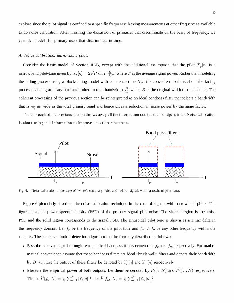
Fig. 6. Noise calibration in the case of ‘white’, stationary noise and ‘white’ signals with narrowband pilot tones.

Figure 6 pictorially describes the noise calibration technique in the case of signals with narrowband pilots. The

figure plots the power spectral density (PSD) of the primary signal plus noise. The shaded region is the noise

PSD and the solid region corresponds to the signal PSD. The sinusoidal pilot tone is shown as a Dirac delta in

the frequency domain. Letfp be the frequency of the pilot tone andfm 6= fp be any other frequency within the

channel. The noise-calibration detection algorithm can be formally described as follows:

• Pass the received signal through two identical bandpass filters centered atfp andfm respectively. For mathe-

matical convenience assume that these bandpass filters are ideal “brick-wall” filters and denote their bandwidth

by BBPF . Let the output of these filters be denoted byYp[n] andYm[n] respectively.

• Measure the empirical power of both outputs. Let them be denoted by P (fp, N) and P (fm, N) respectively.

That is P (fp, N) = 1N

∑Nn=1 |Yp[n]|2 and P (fm, N) = 1

N

∑Nn=1 |Ym[n]|2.

14

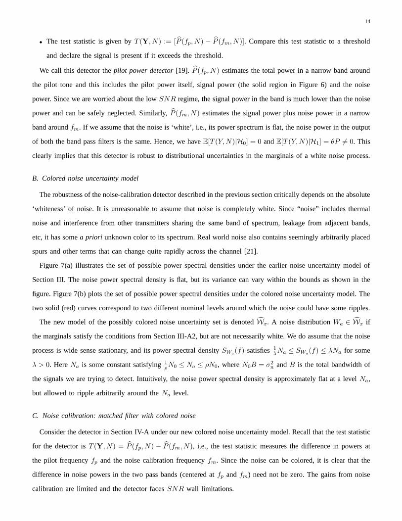
• The test statistic is given byT (Y, N) := [P (fp, N) − P (fm, N)]. Compare this test statistic to a threshold

and declare the signal is present if it exceeds the threshold.

We call this detector thepilot power detector[19]. P (fp, N) estimates the total power in a narrow band around

the pilot tone and this includes the pilot power itself, signal power (the solid region in Figure 6) and the noise

power. Since we are worried about the lowSNR regime, the signal power in the band is much lower than the noise

power and can be safely neglected. Similarly,P (fm, N) estimates the signal power plus noise power in a narrow

band aroundfm. If we assume that the noise is ‘white’, i.e., its power spectrum is flat, the noise power in the output

of both the band pass filters is the same. Hence, we haveE[T (Y, N)|H0] = 0 andE[T (Y, N)|H1] = θP 6= 0. This

clearly implies that this detector is robust to distributional uncertainties in the marginals of a white noise process.

B. Colored noise uncertainty model

The robustness of the noise-calibration detector describedin the previous section critically depends on the absolute

‘whiteness’ of noise. It is unreasonable to assume that noise is completely white. Since “noise” includes thermal

noise and interference from other transmitters sharing thesame band of spectrum, leakage from adjacent bands,

etc, it has somea priori unknown color to its spectrum. Real world noise also contains seemingly arbitrarily placed

spurs and other terms that can change quite rapidly across the channel [21].

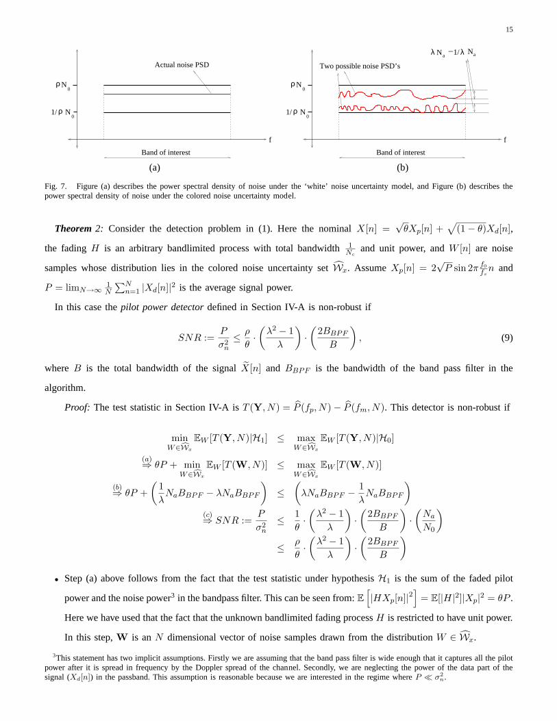
Figure 7(a) illustrates the set of possible power spectral densities under the earlier noise uncertainty model of

Section III. The noise power spectral density is flat, but its variance can vary within the bounds as shown in the

figure. Figure 7(b) plots the set of possible power spectral densities under the colored noise uncertainty model. The

two solid (red) curves correspond to two different nominal levels around which the noise could have some ripples.

The new model of the possibly colored noise uncertainty set isdenotedWx. A noise distributionWa ∈ Wx if

the marginals satisfy the conditions from Section III-A2, but are not necessarily white. We do assume that the noise

process is wide sense stationary, and its power spectral density SWa(f) satisfies1

λNa ≤ SWa(f) ≤ λNa for some

λ > 0. HereNa is some constant satisfying1ρN0 ≤ Na ≤ ρN0, whereN0B = σ2n andB is the total bandwidth of

the signals we are trying to detect. Intuitively, the noise power spectral density is approximately flat at a levelNa,

but allowed to ripple arbitrarily around theNa level.

C. Noise calibration: matched filter with colored noise

Consider the detector in Section IV-A under our new colored noise uncertainty model. Recall that the test statistic

for the detector isT (Y, N) = P (fp, N) − P (fm, N), i.e., the test statistic measures the difference in powersat

the pilot frequencyfp and the noise calibration frequencyfm. Since the noise can be colored, it is clear that the

difference in noise powers in the two pass bands (centered atfp andfm) need not be zero. The gains from noise

calibration are limited and the detector facesSNR wall limitations.

15

1/ρ N0

N0

ρ

f

Band of interest

Actual noise PSD

1/ρ N0

N0

ρ

Naλ Na1/λ−

f

Band of interest

Two possible noise PSD’s

(a) (b)

Fig. 7. Figure (a) describes the power spectral density of noise underthe ‘white’ noise uncertainty model, and Figure (b) describes thepower spectral density of noise under the colored noise uncertainty model.

Theorem 2: Consider the detection problem in (1). Here the nominalX[n] =√

θXp[n] +√

(1 − θ)Xd[n],

the fadingH is an arbitrary bandlimited process with total bandwidth1Ncand unit power, andW [n] are noise

samples whose distribution lies in the colored noise uncertainty setWx. AssumeXp[n] = 2√

P sin 2π f0

fsn and

P = limN→∞1N

∑Nn=1 |Xd[n]|2 is the average signal power.

In this case thepilot power detectordefined in Section IV-A is non-robust if

SNR :=P

σ2n

≤ ρ

θ·(

λ2 − 1

λ

)·(

2BBPF

B

), (9)

where B is the total bandwidth of the signalX[n] and BBPF is the bandwidth of the band pass filter in the

algorithm.

Proof: The test statistic in Section IV-A isT (Y, N) = P (fp, N) − P (fm, N). This detector is non-robust if

minW∈cWx

EW [T (Y, N)|H1] ≤ maxW∈cWx

EW [T (Y, N)|H0]

(a)⇒ θP + minW∈cWx

EW [T (W, N)] ≤ maxW∈cWx

EW [T (W, N)]

(b)⇒ θP +

(1

λNaBBPF − λNaBBPF

)≤

(λNaBBPF − 1

λNaBBPF

)

(c)⇒ SNR :=P

σ2n

≤ 1

θ·(

λ2 − 1

λ

)·(

2BBPF

B

)·(

Na

N0

)

≤ ρ

θ·(

λ2 − 1

λ

)·(

2BBPF

B

)

• Step (a) above follows from the fact that the test statistic under hypothesisH1 is the sum of the faded pilot

power and the noise power3 in the bandpass filter. This can be seen from:E[|HXp[n]|2

]= E[|H|2]|Xp|2 = θP .

Here we have used that the fact that the unknown bandlimited fading processH is restricted to have unit power.

In this step,W is anN dimensional vector of noise samples drawn from the distribution W ∈ Wx.

3This statement has two implicit assumptions. Firstly we are assuming that the band pass filter is wide enough that it captures all the pilotpower after it is spread in frequency by the Doppler spread of the channel. Secondly, we are neglecting the power of the data part of thesignal (Xd[n]) in the passband. This assumption is reasonable because we are interested in the regime whereP ≪ σ2

n.

16

• Step (b) is obtained by using the fact that the minimum difference in noise powers in the two bands is(

1λN0BBPF − λN0BBPF

). Similarly, the maximum possible difference in noise powersin the two bands is

(λN0BBPF − 1

λN0BBPF

).

• (c) follows from the fact thatN0B = σ2n. The final factor ofρ is just present to account for the fact thatNa

N0

could be as big asρ. This is an artifact of the fact that we are expressing the wallin terms of the nominal

SNR and the uncertainty is modeled multiplicatively.

From Theorem 2, it is clear that thepilot power detector’sSNR wall goes to zero as(

BBP F

B

)→ 0. So, can

the bandwidthBBPF of the bandpass filter be reduced arbitrarily? Recall that in the proof of Theorem 2, we

assumed that the pilot power under the bandpass filter isθP . This assumption is true only if the bandpass filter

has a bandwidth greater than the bandwidth of the fading process. This is because the pilot tone is a Dirac delta

in frequency domain and is smeared out due to the fading process. The pilot power is spread over the bandwidth

of the fading process in some unknown way. Therefore, the result of the theorem is true only ifBBPF ≥ 1Nc

. In

fact, tightening the bandpass filter any further could resultin the loss of all the pilot power and missed detection.

Hence the best possibleSNR wall for the pilot power detector is given byρθ ·(

λ2−1λ

)·(

2Nc

).

Notice that in this model of coloring uncertainty, there is no real benefit from calibrating the noise using nearby

frequencies. All frequencies within the channel are considered equally good. This makes physical sense if the

dominant coloring uncertainty is coming from potential local spurs and nulls in the noise. Otherwise, it is easy to

alter the uncertainty model to include some sense of continuity for the noise PSD. In that case, theλ uncertainty

parameter would also be proportional to1Ncsince it is the bandwidth of the fading process that limits how close in

frequency the calibration filter can come. That would result inthe SNR Wall improving asO( 1N2

c

) with increasing

coherence timeNc.

Finally, it is easy to see that the above noise calibration strategy does not really depend on the width of the

bandpass filter used for calibration. Even if it used all the information outside of a tight window containing the

pilot signal, a detector cannot completely calibrate the noise process within that tight window due to the unknown

color. Within that tight window, all detectors essentiallyface the same problem as Theorem 1 — an arbitrary (and

hence possibly white) signal in the presence of noise with a residual unknown level coming from the color ripple.

D. Noise calibration: 50% duty cycle pulse amplitude modulated signals

It is immediately obvious that Theorem 2 also generalize to cases where the primary signal restricts itself

to use aβ fraction of the bandwidth. This gives a processing gain corresponding to the bandwidth restriction

BBPF = (β + 1Nc

)B and setsθ = 1, but otherwise introduces no qualitatively new concerns. In that case, the

17

coherence time plays no significant role in the SNR wall. The noise calibration gains add to the bandwidth reduction

gains in a straightforward way.

We now explore another approach to using only some of the underlying degrees of freedom. To be specific,

consider an example signal that uses only half of the available degrees of freedom intime rather than frequency.

X[n] =

±√

2P w. p. 12 if n is odd,

0 if n is even.(10)

The average power of this signal isP and this example is a caricature of practical signals whose amplitude is

modulated using time domain pulses. Such pulse amplitude modulated signals come under the general category

of cyclostationarysignals [22]–[24].Feature detectorsare a general class of detectors that have been proposed to

distinguish cyclostationary signals from noise. These detectors were first proposed by William Gardner [25], [26].

Robustness of feature detectors is an active topic of research in this area. Fundamental results on robustness of

single cyclefeature detectors are shown in [27], [28], but here we illustrate the basic ideas in the context of this

simple caricature.

As in (1), the received signal under hypothesisH1 can be written asY [n] = HX[n]+W [n], whereW [n]’s are the

noise samples whose distribution lies in the uncertainty set Wx. In this example, the average power measurements

at ‘even’ time samples can be used to calibrate the noise in the ‘odd’ time samples.

1) No fading: Suppose that there was no fading. The natural test statistic isgiven by

T (Y) =

[1

N

N∑

n=1

|Y [2n − 1]|2 − 1

N

N∑

n=1

|Y [2n]|2]

. (11)

In this case it is easy to verify thatE[T (Y)|H0] = E[ 1N

∑Nn=1 |W [2n − 1]|2] − E[ 1

N

∑Nn=1 |W [2n]|2] = 0 and

E[T (Y)|H1] = 2P 6= 0. Therefore, it is clear that we can obtain infinite gains from noise calibration and hence

there is noSNR wall if the noise is guaranteed to be white. The somewhat surprising fact here is that the same is

true even if the the noise is colored. The mean of the test statistic is still the difference of two expectations. The

noise contribution to each expectation is identical bystationarity, not whiteness.

2) Flat fading: Assume that the channel fading is flat (i.eH is just multiplication by a bandlimited scalar signal).

For pilot-detection, this is enough to cause an SNR wall sinceit spreads the pilot tone over a finite bandwidth and

thereby stops infinite coherent processing gains. In this case however, the scalar multiplication can do nothing to

the zero samples of the signal! Even time-samples continue toprovide a clean view of the noise. Therefore, by the

arguments above the noise calibration becomes perfect. Noise color is not enough to stop this since the stationarity

and presumed ergodicity of the noise guarantees that the calibration term 1N

∑Nn=1 |Y [2n]|2 = 1

N

∑Nn=1 |W [2n]|2

converges with probability one to1N∑N

n=1 |W [2n − 1]|2 asN gets large.

18

3) Frequency-selective fading:The previous result is somewhat surprising since the matchedfilter for pilot

tones is not-robust to this kind of flat-fading uncertainty, even with noise calibration when the noise is colored.

However, frequency-selective fading does introduce an SNR wall for this detector. To illustrate the idea, consider

the simplest possible frequency-selective fading: a delay. Let the received signal under hypothesisH1 be Y [n] =

X[n − l[n]] + W [n].

Here, the traditional notion of a bandlimited fading process is inadequate to capture the size of the relevant

uncertainty. After all, the arguments of the previous section suggest thatHX[n] = h[n]X[n − l[n]] would behave

the same as justX[n− l[n]] while the apparent bandwidth of the fading process might be dominated by a fast flat

component given byh[n]. Instead, consider a block-fading model in which the delayl[n] is piecewise constant for

Dc time steps before taking on an independent realization. Call Dc the lower bound on thedelay coherence time.

To understand the nature of the delay coherence timeDc, it is useful to consider two cases:

• Assume that the delay spread of the channel is significantly larger than1 sample and all of the channel taps

arise from the sum of many paths. (There is no dominant line-of-sight path) As these path-lengths change over

time, all of the taps will get different values. In such a case, the delay coherence timeDc and the traditional

amplitude coherence timeNc (or equivalently, the reciprocal of the bandwidth of the fading process) are the

same since the relative phase response can change significantly in this time. This is the model that is likely to

hold for wideband primary users being detected at significantdistances from their transmitters. This basically

corresponds to when ISI is significant.

• Now suppose there is only one dominant line-of-sight path that is arriving at the spectrum sensor, but is subject

to local reflections in the near neighborhood of the sensor. (e.g. A user in an airplane) The delay spread of the

channel can be smaller than1 sample. In this case, there will just be a single tap in the filter. The amplitude

might change rapidly since the local paths can go in and out ofphase with each other, but the overall delay

is not going to be changing as fast. In such cases, the delay coherence timeDc > Nc and the dominant effect

may very well be the clock skew of the sensor’s local oscillator relative to the primary oscillator. In such cases,

the factor difference betweenDc andNc is comparable to the factor difference between the signal bandwidth

and the carrier frequency.

For this simplest example of a fading process with finiteDc, the strategy of (11) is doomed to failure if the sums

are taken beyond one coherence time. The signal will corrupt both the even and odd time samples eventually due

to the random delay. By analogy with the case of matched filtering, a natural detection strategy is to compute the

square of the test statistic within each coherence time and average that over multiple coherence times. The modified

19

test statistic is given by

T (Y, Dc) =1

M

M−1∑

k=0

∣∣∣∣∣∣2

Dc

Dc/2∑

n=1

{|Y [kM + 2n − 1]|2 − |Y [kM + 2n]|2

}∣∣∣∣∣∣

2 , (12)

whereN = MDc.

Theorem 3: Let the received signal under hypothesisH1 in (1) be given byY [n] = X[n − l[m]] + W [n], with

X[n] given in (10), andW [n] stationary uncertain noise independent of the signal. Assume that the distribution of

the noise arises from the noise uncertainty setWx. Suppose the delay fading satisfies:

• l[m] is constant within a delay coherence block andiid across different delay coherence blocks.

• l[m] is uniformly distributed on{0, 1}.

Define,SNR = Pσ2

n

. The detector defined in (12) is non-robust if

SNR ≤−2ρ + 2

√1ρ2 + (2 + Dc)(ρ2 − 1

ρ2 )

2 + Dc, where ρ = 10

x

10 .

Proof: From (12) it is clear that

E[T (Y, Dc)|Hi] = E

∣∣∣∣∣∣2

Dc

Dc/2∑

n=1

{|Y [2n − 1]|2 − |Y [2n]|2

}∣∣∣∣∣∣

2∣∣Hi

, for i = 0, 1. (13)

The following lemma gives the desired quantities.

Lemma 1:

E[T (Y, Dc)|H0] =16σ4

Dc, E[T (Y, N)|H1] = 4P 2 +

16σ4 + 16Pσ2 + 8P 2

Dc, (14)

whereW [n] ∼ N (0, σ2).

Proof: See Appendix C.

Using Lemma 1, it is clear that the detector in (12) is non-robust if the set of means under both hypotheses

overlap. This condition is equivalent to

min1

ρσ2

n≤σ2≤ρσ2n

4P 2 +16σ4 + 16Pσ2 + 8P 2

Dc≤ max

1

ρσ2

n≤σ2≤ρσ2n

16σ4

Dc

⇒ P 2 +4 1

ρ2 σ4n + 4P 1

ρσ2n + 2P 2

Dc≤ 4ρ2σ4

n

Dc

The last inequality inSNR := Pσ2

n

can be solved to give the required result by the quadratic formula.

This theorem suggests that it is the uncertainty corresponding to the frequency selectivity of the fading that induces

limits on the detection of very weak signals that do not fullyutilize all the degrees of freedom in time-domain.

There are two interesting aspects of this result:

20

• The dependence of the SNR wall for this detector on the delay coherence time isO( 1√Dc

). This gain from

increasing delay coherence time is slower than theO( 1Nc

) gain for the matched filter, but itis better than the

lack of any gain with coherence time for a primary signal thatonly uses half the degrees of freedom in the

frequency domain.

• The SNR wall result so far does not depend on the color of the noise! The proposed detector in (12), while

being intuitively very natural, is non-robust in the presence of frequency-selective fading, even when the noise

is truly white. A consequence of this is that the SNR wall depends only onρ, not on the potentially much

smallerλ. As the next section shows, this is an artifact of the detection strategy used.

E. Noise calibration: color revisited

The intuitively natural detector from (12) seems to be doing noise calibration, but Theorem 3 shows that it gets

no improvements in the SNR Wall from reducedλ ripples in the noise color. This prompts the question whether

the detector in (12) is even close to the best possible detector for exploiting noise calibration gains?

While the question remains open in general, it turns out thatdetectors based on cyclostationary feature detection

behave similarly to the detector (12) and thus do not seem to be able to fully exploit the promise of noise calibration

[27], [28]. However, itis possible to give an example of a better detector that is motivated from information-theoretic

arguments coming from the method of types [29]. Consider thefollowing detection algorithm:

• Within each delay coherence block, compute the empirical average power of the odd samples and even samples.

That is, compute(Pk,odd(Dc), Pk,even(Dc)), where

Pk,odd(Dc) =2

Dc

Dc2∑

n=1

|Y [kDc + 2n − 1]|2, Pk,even(Dc) =2

Dc

Dc2∑

n=1

|Y [kDc + 2n]|2

• Quantize these average powers into two bins using a global quantization thresholdT — i.e. setBk,odd(Dc) = 1

if Pk,odd(Dc) ≥ T and zero otherwise. Similarly forBk,even(Dc).

• Collect these quantized pairs(Bk,odd(Dc), Bk,odd(Dc)) for k = 1, 2, · · · , K, for a very large number of delay

coherence blocksK.

• Compute the empirical distribution of theunorderedbinary pairs{Bk,odd(Dc), Bk,odd(Dc)}, k = 1, 2, · · · , K.

Denote this empirical probability distribution(p11(K), p10(K), p00(K)).

• Choose the global thresholdT so thatp11(K) = 14 . From a practical point of view, this can be thought of as

a kind of automatic gain control (AGC) that is set so that the quantizer sees the pair(1, 1) a fourth of the

time. In a sense, this AGC is implicitly doing calibration tothe noise.

• The test statistic isp00(K) and the detector declares hypothesisH0 if | limK→∞ p00(K) − 14 | ≤ δ for some

small thresholdδ > 0, and declaresH1 otherwise.

21

Note that under either hypothesisHi, i = 0, 1, the empirical probabilities(p11(K), p10(K), p00(K)) converge to

their true probabilities asK → ∞. The key question is what are the possible limiting probability distributions as

the noise distribution varies over the noise uncertainty set Wx?

1) Under hypothesisH0 and white noise:The distributions of both the odd and even samples are independent

and identical. This implies thatBk,odd(Dc) is also independent and identical toBk,even(Dc). This forces the limiting

empirical distribution to have the following form:

limK→∞

(p11(K), p10(K), p00(K)) = (p2, 2p(1 − p), (1 − p)2),

wherep = Prob(Pk,odd(Dc) ≥ T |H0) = Prob(Pk,even(Dc) ≥ T |H0). Furthermore, since the AGC is set such that

the probability of a(1, 1) is 14 , we must havep = 1

2 , and hence the limiting distribution is(14 , 1

2 , 14).

2) Under hypothesisH1 and white noise: In this case, the distributions of the odd and even samples are

independent but not identical. This is because one of the two has more energy than the other (since it has both

signal plus noise). Therefore, the limiting distribution isof the form

limK→∞

(p11(K), p10(K), p00(K)) = (qr, q(1 − r) + r(1 − q), (1 − q)(1 − r)),

for some0 ≤ q ≤ 1, 0 ≤ r ≤ 1 given by

q = Prob(Pk,odd(Dc) ≥ T |H1), r = Prob(Pk,even(Dc) ≥ T |H1).

where the delayl[n] = 0 for the purposes of calculatingq, r underH1. Furthermore, the AGC is set so thatqr = 14 .

To have the hypotheses overlap, we would have to be able to also setq(1 − r) + r(1 − q) = 12 which implies that

q + r = 1. But the geometric mean and arithmetic means ofq, r can only agree ifq = r = 12 which is not possible

if there is any signal present.

This immediately shows that the limiting empirical probability distributions under both hypotheses are disjoint

if the noise is truly white. Hence, we can always separate thetwo hypotheses and this detector is robust to ‘white’

noise level uncertainties regardless of how short the delaycoherence timeDc ≥ 2 is. This result is consistent with

our intuition that ‘white’ noise level uncertainties are insufficient to limit noise calibration gains.

3) Under colored noise:For ease of analysis, consider a specific colored Gaussian noise uncertainty model. Let

M [n] be aniid white Gaussian noise process, with the varianceσ2m ∈ [1ρσ2

n, ρσ2n]. DefineW [n] = M [n]−αM [n−1]

for someα > 0. Suppose that just theα is unknown to within some small range0 ≤ α ≤ αmax.

The two-dimensional central limit theorem can be applied to(G1, G2) := (bPk,odd(Dc)

√Dc

2σ2m

,bPk,even(Dc)

√Dc

2σ2m

). Stan-

dard calculations reveal that this approaches a jointly normal random variable with variances(1+α2)2 and covari-

22

ance4 2α2. The means underH0 are((1+α2)√

Dc

2 , (1+α2)√

Dc

2 ) and are((1+α2)√

Dc

2 , (1+α2)√

Dc

2 +SNR√

Dc)

underH1. The variances and covariance do not change substantially inH1 whenP is small relative toσ2m.

The limiting distribution for the test statistic is thus

limK→∞

(p11(K), p10(K), p00(K)) = (1

4, aα, bα),

for someaα + bα = 34 .

For the noise-only hypothesis, if the noise is white, then clearlya0 = 12 andb0 = 1

4 . Otherwise for the noise-only

case, it is clear5 that bα ≈ 14 + K1α

2 for some constantK1 when α is small. When the signal is present, then

bα ≈ 14 + K1α

2 − K2SNR2Dc with K2 being another constant6 whenα is small. Thus, the presence or absence

of the signal is robustly detectable only ifSNR > K3αmax√

Dc

for some constantK3. This recovers theO(

1√Dc

)

scaling in the SNR wall, but also includes a clear dependence on the coloring parameter7 αmax.

We conjecture that this detector is order optimal in terms ofthe dependence on the coloring parameter and the

delay coherence time. However it is clear that the noise-calibration gains are intimately tied up with the features

of the signaling itself.

V. THE CAPACITY-ROBUSTNESS TRADEOFF

It is natural to wonder ‘Who must pay the price for robust detection?’ The goal of the primary transmitter is to

maximize its data rate to the primary receiver, while the secondary user wants to be able to design a robust algorithm

to detect the presence of the primary. The relevant tradeoff is between the performance loss to the primary system

and the robustness gains to the secondary system. The primaryperformance can be quantified using capacity and

this paper’s results indicate that robustness can be quantified in terms of the SNR wall.

For a target SNR wall, the ultimate goal is to find a primary signaling scheme that maximizes the data rate

achievable to the primary system while still being robustlydetectable above the wall. Conversely, given a target

primary data rate, the goal is to find the primary signaling scheme that maximizes the robustness of secondary

detection. If the primary were only concerned with a given bandwidth and power constraint, then information

theory reveals that the optimal signaling should look white[29] and Theorem 1 indicates that this gives very poor

robustness for the secondary. Thus, it appears that this tradeoff is fundamental from a system design point of view

and can be called the ‘capacity-robustness tradeoff’.

4It is clear that even under a general model for colored wide-sense stationary noise, the covariance here is going to be a function ofthe amount of coloring since it captures a particular way in which the noise deviates fromiid. The positive correlation here obscures theseparation of the two quantities if the signal is present.

5Space reasons force us to omit the proof. Intuitively, just think of the joint Gaussian as being the sum of a pair of two iid Gaussianrandom variables(N1, N2) with an independent pair distributed like(+Nα, +Nα). The variance ofNα is proportional toα2.

6The constant acts negatively since having a signal present tends to make the two move in opposite directions and hence reduces theprobability that both cross the threshold.

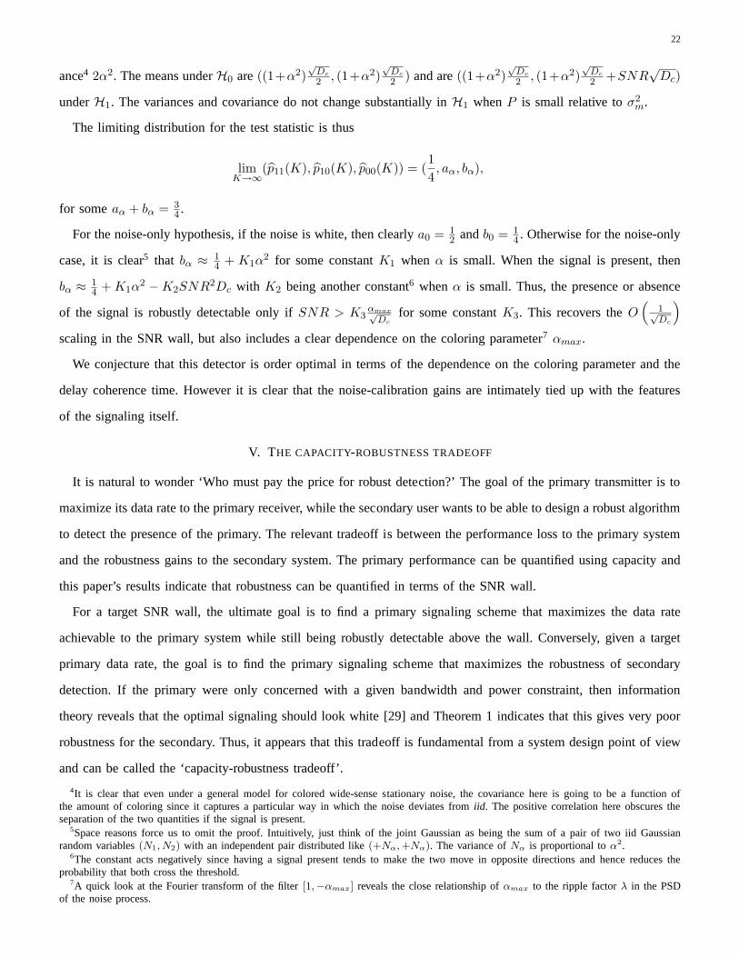
7A quick look at the Fourier transform of the filter[1,−αmax] reveals the close relationship ofαmax to the ripple factorλ in the PSDof the noise process.

23

It is a non-trivial open problem to determine the optimal tradeoff. Instead, here the tradeoff is explored in the

context of a given sensing algorithm and class of primary signals.

A. Capacity-robustness tradeoff: energy detector

Let the channel between the primary transmitter and primary receiver be a classic bandlimited AWGN channel.

The capacity of this channel is completely characterized by the channel bandwidthB and the signal to noise ratio

SNRP = PP

N0B, wherePP is the received signal power at the primary receiver andN0 is the noise power spectral

density. The capacity is given byC = B log (1 + SNRP ) assuming complex signaling. Assume that the spectrum

sensor uses a radiometer to detect the primary signal. As seen in Section III-A, the relevantSNRenergywall = ρ2−1

ρ .

The SNR at the sensor can be written asSNRS = PS

N0B, wherePS is the received primary power at the spectrum

sensor.

It is clear that the common parameter that affects both the primary data rate and the sensingSNR is the bandwidth

B. The primary transmitter can tradeoff its rate in exchange for robustness at the spectrum sensor by reducing the

fraction of degrees of freedom used. LetBactual = βB, whereβ ∈ (0, 1). We also assume that the fading at the

spectrum sensor is bandlimited and has a bandwidth ofBNc

. In this case, the total bandwidth potentially occupied

by the primary signal at the spectrum sensor isβB + BNc

. The effective SNR wall is given by(β + 1Nc

)(

ρ2−1ρ

).

Hence the capacity-robustness tradeoff for the simple radiometer is given by the parametric curve

(robustness, capacity) :

[(β +

1

Nc)

(ρ2 − 1

ρ

), βB log

(1 +

PP

βN0B

)], (15)

whereβ ∈ [0, 1]. The factorβ in the robustness is the processing gain obtained because the primary does not use

all the degrees for freedom.

One can also obtain noise calibration gains by taking measurements in the frequencies over which the primary

does not spread its signal. Using the model in Section IV-B, the uncertainty in the noise is reduced fromρ to some

smaller numberλ. Therefore, the tradeoff with noise calibration is given by:

(robustness, capacity) :

[(β +

1

Nc)ρ

(λ2 − 1

λ

), βB log

(1 +

PP

βN0B

)]. (16)

B. Capacity-robustness tradeoff: coherent detector

Assume that the spectrum sensor uses a coherent detector andthe primary signal has a deterministic pilot

tone as in Section III-B. Any power spent on the pilot improvesrobustness but reduces the power available for

communicating messages. Letθ be the fraction of total power spent in the pilot tone. The primary data rate is

bounded byRP = B log(1 + (1−θ)PP

N0B

). From (8), the SNR wall is given bySNR

mfwall = 1

Nc·θ

(ρ2−1

ρ

), where

24

θ ∈ [0, 1] and Nc is the channel coherence time. Thus, the capacity-robustness tradeoff for the matched filter is

given by the parametric curve

(robustness, capacity) :

[1

Nc · θ

(ρ2 − 1

ρ

), B log

(1 +

(1 − θ)PP

N0B

)], (17)

whereθ ∈ [0, 1]. The gains in robustness given in (17) are coherent processing gains. As discussed in Section IV-C,

noise calibration can also be used to reduce the uncertaintydown to theλ level. Hence, the capacity-robustness

tradeoff with noise calibration is given by

(robustness, capacity) :

[ρ

Nc · θ

(λ2 − 1

λ

), B log

(1 +

(1 − θ)PP

N0B

)], (18)

C. Numerical examples

−15 −10 −5 0 5 100

1

2

3

4

5

6

SNR wall (in dB)

Prim

ary

data

rate

(in

Mbp

s)

Capacity robustness tradeoffs

Matched filterMatched filter with noise calibrationEnergy detectorEnergy detection with noise calibration

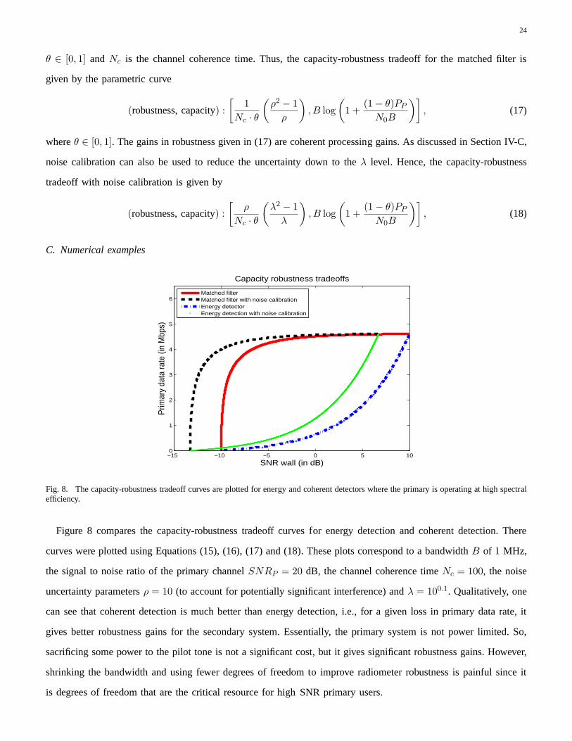
Fig. 8. The capacity-robustness tradeoff curves are plotted for energy and coherent detectors where the primary is operating at high spectralefficiency.

Figure 8 compares the capacity-robustness tradeoff curves for energy detection and coherent detection. There

curves were plotted using Equations (15), (16), (17) and (18). These plots correspond to a bandwidthB of 1 MHz,

the signal to noise ratio of the primary channelSNRP = 20 dB, the channel coherence timeNc = 100, the noise

uncertainty parametersρ = 10 (to account for potentially significant interference) andλ = 100.1. Qualitatively, one

can see that coherent detection is much better than energy detection, i.e., for a given loss in primary data rate, it

gives better robustness gains for the secondary system. Essentially, the primary system is not power limited. So,

sacrificing some power to the pilot tone is not a significant cost, but it gives significant robustness gains. However,

shrinking the bandwidth and using fewer degrees of freedom to improve radiometer robustness is painful since it

is degrees of freedom that are the critical resource for highSNR primary users.

25

−15 −10 −5 0 5 100

0.05

0.1

0.15

SNR wall (in dB)

Prim

ary

data

rate

(in

Mbp

s)

Capacity robustness tradeoffs

Matched filterMatched filter with noise calibrationEnergy detectorEnergy detection with noise calibration

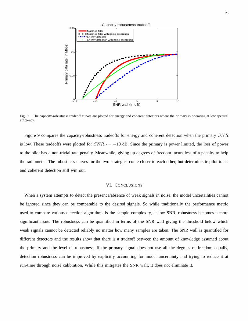
Fig. 9. The capacity-robustness tradeoff curves are plotted for energy and coherent detectors where the primary is operating at low spectralefficiency.

Figure 9 compares the capacity-robustness tradeoffs for energy and coherent detection when the primarySNR

is low. These tradeoffs were plotted forSNRP = −10 dB. Since the primary is power limited, the loss of power

to the pilot has a non-trivial rate penalty. Meanwhile, giving up degrees of freedom incurs less of a penalty to help

the radiometer. The robustness curves for the two strategiescome closer to each other, but deterministic pilot tones

and coherent detection still win out.

VI. CONCLUSIONS

When a system attempts to detect the presence/absence of weak signals in noise, the model uncertainties cannot

be ignored since they can be comparable to the desired signals. So while traditionally the performance metric

used to compare various detection algorithms is the sample complexity, at low SNR, robustness becomes a more

significant issue. The robustness can be quantified in terms of the SNR wall giving the threshold below which

weak signals cannot be detected reliably no matter how many samples are taken. The SNR wall is quantified for

different detectors and the results show that there is a tradeoff between the amount of knowledge assumed about

the primary and the level of robustness. If the primary signal does not use all the degrees of freedom equally,

detection robustness can be improved by explicitly accounting for model uncertainty and trying to reduce it at

run-time through noise calibration. While this mitigates the SNR wall, it does not eliminate it.

26

APPENDIX A

PROOF OFTHEOREM 1

For k ≥ 1, definef(k, SNR) to be the following uni-variate degreek polynomial

f(k, SNR) :=

[k∑

i=0

(2k

2k − 2i

)(1

ρk−i

)(1 · 3 · 5 · · · (2k − 2i − 1)

1 · 3 · 5 · · · (2k − 1)

)SNRi

]. (19)

Note that all the coefficients off(k, SNR) are non-negative and hencef(k, SNR) is monotonically increasing

in SNR. This means that the equationf(k, SNR) = ρk has a unique real valued rootSNR(2k)wall. Becausef(k, 0) =

1ρk < ρk sinceρ > 1, the rootSNR

(2k)wall > 0 for all k. DefineSNR∗

wall to be

SNR∗wall := inf

k=1,2,3,···∞SNR

(2k)wall. (20)

Let Wn ∼ N (0, σ2n), W1 ∼ 1√

ρWn. Let W2 := X + W1. If W1 ∈ Wx, andW2 ∈ Wx, then it is clear that robust

detection is impossible. We now prove thatW2 ∈ Wx by showing thatEW 2k−12 = 0 and 1

ρk EW 2kn ≤ EW 2k

2 ≤

ρkEW 2kn ∀ k.

SinceE[X2k−1] = 0 andW2 =: X + W1, we haveEW 2k−12 = 0 andEW 2k

2 ≥ 1ρk EW 2k

n . Therefore,W2 ∈ Wx

⇔ EW 2k2 ≤ ρk EW 2k

n

⇔ E(X + W1)2k

EW 2kn

≤ ρk

⇔k∑

i=0

(2k

2k − 2i

)EW 2k−2i

1

EW 2kn

EX2i ≤ ρk

⇔k∑

i=0

(2k

2k − 2i

)(1

ρk−i

)(1 · 3 · 5 · · · (2k − 2i − 1) σ2k−2i

n

1 · 3 · 5 · · · (2k − 1) σ2kn

)EX2i ≤ ρk

⇔k∑

i=0

(2k

2k − 2i

)(1

ρk−i

)(1 · 3 · 5 · · · (2k − 2i − 1)

1 · 3 · 5 · · · (2k − 1)

)EX2i

σ2in

≤ ρk ∀ k = 1, 2, · · · (21)

So, we just need to show that the last inequality in (21) is true.

By definition of ‘peakSNR’, we have EX2i

σ2in

≤ SNRipeak. Now, if SNRpeak ≤ SNR∗

wall, by the monotonicity

of f(k, SNR), we have

k∑

i=0

(2k

2k − 2i

) (1

ρk−i

) (1 · 3 · 5 · · · (2k − 2i − 1)

1 · 3 · 5 · · · (2k − 1)

)EX2i

σ2in

≤k∑

i=0

(2k

2k − 2i

) (1

ρk−i

) (1 · 3 · 5 · · · (2k − 2i − 1)

1 · 3 · 5 · · · (2k − 1)

)SNRi

peak

= f(k, SNRpeak)

≤ f(k, SNR∗wall) = ρk.

27

which is the last inequality in (21).

In terms of the upper-bound in (7), from (20) it is clear thatSNR∗wall ≤ SNR

(2)wall = ρ2−1

ρ . However, the entire

result is vacuous if the infimum in (20) is zero. Getting a nontrivial lower bound is more interesting.

Recall thatSNR(2k)wall is the root of the polynomialf(k, SNR)−ρk. The coefficient ofSNRi in f(k, SNR)−ρk

is(

2k2k−2i

) (1

ρk−i

) (1·3·5···(2k−2i−1)

1·3·5···(2k−1)

). Replace

(1

ρk−i

)by 1 to get a new polynomial,f(k, SNR)− ρk. Sinceρ > 1,

we have(

1ρk−i

)≤ 1 for all i = 1, 2, · · · , k, and hence the unique positive root off(k, SNR) − ρk = 0 must be

smaller thanSNR(2k)wall. Call this rootSNR

(2k)

wall.

It is thus clear that

SNR∗wall ≥ inf

k=1,2,··· ,∞SNR

(2k)

wall (22)

whereSNR(2k)

wall is the unique positive root of

f(k, SNR) :=

[k∑

i=0

(2k

2k − 2i

)(1 · 3 · 5 · · · (2k − 2i − 1)

1 · 3 · 5 · · · (2k − 1)

)SNRi

]= ρk. (23)

This polynomial has a natural upper bound given in the following lemma.

Lemma 2:

f(k, SNR) ≤ (1 + SNR)k, ∀ k ≥ 1, SNR ≥ 0

Proof: See Appendix B.

Using the above lemma in (23) gives

ρk = f(k, SNR(2k)

wall)

≤ (1 + SNR(2k)

wall)k.

This implies that

SNR(2k)

wall ≥ ρ − 1, ∀ k ≥ 1.

Substituting the above inequality in (22) gives the desired lower bound.

28

APPENDIX B

PROOF OF LEMMA 2

Fix k ≥ 1 andSNR ≥ 0. From the definition off(k, SNR) in (23), we get

f(k, SNR) =

[k∑

i=0

(2k

2k − 2i

)(1 · 3 · 5 · · · (2k − 2i − 1)

1 · 3 · 5 · · · (2k − 1)

)SNRi

]

=

[k∑

i=0

(2k)!

(2k − 2i)! · (2i)!

(1 · 3 · 5 · · · (2k − 2i − 1)

1 · 3 · 5 · · · (2k − 1)

)SNRi

]

=

[k∑

i=0

(2k) · (2k − 1) · · · (2k − 2i + 1)

(2i) · (2i − 1) · · · 1

(1 · 3 · 5 · · · (2k − 2i − 1)

1 · 3 · 5 · · · (2k − 1)

)SNRi

]

(a)=

[k∑

i=0

(k

i

)(2k − 1) · (2k − 3) · · · (2k − 2i + 1)

(2i − 1) · (2i − 3) · · · 1 · 1 · 3 · 5 · · · (2k − 2i − 1)

1 · 3 · 5 · · · (2k − 1)SNRi

]

(b)=

[k∑

i=0

(k

i

)1

(2i − 1) · (2i − 3) · · · 1SNRi

]

≤[

k∑

i=0

(k

i

)SNRi

]

= (1 + SNR)k.

• (a) follows from the following calculation.

(2k) · (2k − 1) · · · (2k − 2i + 1)

(2i) · (2i − 1) · · · 1 =

((2k) · (2k − 2) · · · (2k − 2i + 2)

(2i) · (2i − 2) · · · 2

)·(

(2k − 1) · (2k − 3) · · · (2k − 2i + 1)

(2i − 1) · (2i − 3) · · · 1

)

=

(2i · (k) · (k − 1) · · · (k − i + 1)

2i · (i) · (i − 1) · · · 1

)·(

(2k − 1) · (2k − 3) · · · (2k − 2i + 1)

(2i − 1) · (2i − 3) · · · 1

)

=

(k

i

)((2k − 1) · (2k − 3) · · · (2k − 2i + 1)

(2i − 1) · (2i − 3) · · · 1

).

• (b) follows from the following calculation.

[(2k − 1) · (2k − 3) · · · (2k − 2i + 1)

(2i − 1) · (2i − 3) · · · 1 · 1 · 3 · 5 · · · (2k − 2i − 1)

1 · 3 · 5 · · · (2k − 1)

]

=

[1

(2i − 1) · (2i − 3) · · · 1 · 1 · 3 · 5 · · · (2k − 1)

1 · 3 · 5 · · · (2k − 1)

]=

[1

(2i − 1) · (2i − 3) · · · 1

].

APPENDIX C

PROOF OF LEMMA 1

Under hypothesisH0: Y [n] = W [n] ∼ N (0, σ2) for all n > 0. Using this in (13), we get

E[T (Y, Dc)|H0] = E

∣∣∣∣∣∣2

Dc

Dc/2∑

n=1

{|W [2n − 1]|2 − |W [2n]|2

}∣∣∣∣∣∣

2 . (24)

29

|W [2n − 1]|2 − |W [2n]|2 are iid random variables with zero mean and variance4σ4. Using the Central Limit

Theorem [15], we get

1√Dc

Dc/2∑

n=1

{|W [2n − 1]|2 − |W [2n]|2

}∼ N (0, 4σ4).

Using this approximation in (24), we getE[T (Y, Dc)|H0] = 16σ4

Dc.

Under hypothesisH1: To compute the expectation of the modified test-statistic in(13) we can assumel[m] = 0

without loss of generality. So, we haveY [2n − 1] = X[2n − 1] + W [2n − 1] ∼ N (0, P + σ2) and Y [2n] =

X[2n] + W [2n] = W [2n] ∼ N (0, σ2) for all n > 0. This implies that|Y [2n − 1]|2 − |Y [2n]|2 are iid random

variables with meanP and variance4σ4 + 4Pσ2 + 2P 2. Again using the Central Limit Theorem [15], we get

1√Dc

Dc/2∑

n=1

{|Y [2n − 1]|2 − |Y [2n]|2

}∼ N (

√DcP, 4σ4 + 4Pσ2 + 2P 2).

Using this approximation we get

E[T (Y, Dc)|H1] = E

∣∣∣∣∣∣2

Dc

Dc/2∑

n=1

{|Y [2n − 1]|2 − |Y [2n]|2

}∣∣∣∣∣∣

2∣∣H1

=4

DcE

∣∣∣∣∣∣1√Dc

Dc/2∑

n=1

{|Y [2n − 1]|2 − |Y [2n]|2

}∣∣∣∣∣∣

2∣∣H1

=4

Dc[4σ4 + 4Pσ2 + 2P 2 + DcP

2]

= 4P 2 +16σ4 + 16Pσ2 + 8P 2

Dc

ACKNOWLEDGMENTS

We thank the NSF ITR program (ANI-0326503) for funding this research. The work is also indebted to ongoing

interactions with Mubaraq Mishra, Danijela Cabric, and Niels Hoven. The anonymous reviewers and issue editor

Akbar Sayeed were immensely helpful in shaping the presentation and scope of this paper.

REFERENCES

[1] FCC, “FCC 04-113,” May 2004. [Online]. Available: http://hraunfoss.fcc.gov/edocspublic/attachmatch/FCC-04-113A1.pdf

[2] V. R. Cadambe and S. A. Jafar, “Interference alignment and thedegrees of freedom for the K user interference channel,”Submitted to

the IEEE Transactions on Information theory, 2007.

[3] N. Devroye, P. Mitran, and V. Tarokh, “Achievable rates in cognitive radio,” IEEE Trans. Inform. Theory, May 2006.

[4] P. Grover and A. Sahai, “On the need for knowledge of the phase inexploring known primary transmissions,” inProc. of 2nd IEEE

International Symposium on New Frontiers in Dynamic Spectrum Access Networks, April 2007.

[5] A. Sahai, N. Hoven, and R. Tandra, “Some fundamental limits on cognitive radio,” in Forty-second Allerton Conference on

Communication, Control, and Computing, Monticello, IL, Oct. 2004.

30

[6] N. Hoven, “On the feasibility of cognitive radio,” Master’s thesis, University of California, Berkeley, 2005.

[7] S. Shellhammer, “Numerical spectrum sensing requirements,” inIEEE 802.22-06/0088r0, June 2006.

[8] C. R. Stevenson, C. Cordeiro, E. Sofer, and G. Chouinard, “Functional requirements for the 802.22 WRAN standard,” inIEEE 802.22-

05/0007r46, September 2005.

[9] S. M. Kay, Fundamentals of statistical signal processing: Detection theory. Printice Hall PTR, 1998, vol. 2.

[10] H. V. Poor,An Introduction to Signal Detection and Estimation, 2nd ed. Springer, March 1998.

[11] A. Sonnenschein and P. M. Fishman, “Radiometric detection of spread-spectrum signals in noise of uncertain power,”IEEE Trans.

Aerosp. Electron. Syst., vol. 28, pp. 654–660, Jul. 1992.

[12] D. Cabric, A. Tkachenko, and R. W. Brodersen, “Experimental study of spectrum sensing based on energy detection and network

cooperation,” in the proceedings of IEEE MILCOM 2006.

[13] P. J. Huber, “A robust version of the probability ratio test,”The Annals of Mathematical Statistics, vol. 36, pp. 1753–1758, 1965.

[14] ——, Robust Statistics. Wiley-Interscience, February 1981.

[15] R. Durrett,Probability: Theory and Examples, 3rd ed. Belmont: Duxbury Press, 2004.

[16] S. Shellhammer and R. Tandra, “Performance of the power detector with noise uncertainty,” in IEEE

802.22-06/0134r0, July 2006. [Online]. Available: ”http://ieee802.org/22/Meetingdocuments/2006July/22-06-0134-00-0000

Performance-of-the-power-detector-with-Noise-Uncertainty.ppt”

[17] ATSC Digital Television Standard, ATSC Std. A/53, 2007. [Online]. Available: ”http://www.atsc.org/standards.html”

[18] R. Tandra, “Fundamental limits on detection in low SNR,” Master’s thesis, University of California, Berkeley, 2005. [Online].

Available: http://www.eecs.berkeley.edu/∼tandra/pub1.htm

[19] S. Shellhammer and R. Tandra, “An evaluation of DTV pilot power detection,” in IEEE 802.22-06/0188r0, September 2006. [Online].

Available: ”http://ieee802.org/22/Meetingdocuments/2006Sept/22-06-0188-00-0000-An-Evaluation-of-DTV-Pilot-Power-Detection.

ppt”

[20] S. Mathur and S. Shellhammer, “An evaluation of the PN sequence based detection of DTV signals in the

draft,” in IEEE 802.22-06/0189r0, September 2006. [Online]. Available: ”http://ieee802.org/22/Meetingdocuments/2006Sept/

22-06-0189-00-0000-An-Evaluation-of-the-PN-Sequence-based-detection-of-DTV-signals.ppt”

[21] N. Agarwal, A. Sahai, and J. Tsitsiklis, “Narrowband noise mitigationin location-determining signal processing,” U.S. Patent 7 177 614,

February, 2007.

[22] W. A. Gardner, “The spectral correlation theory of cyclostationary time-series,”Signal Processing, vol. 11, pp. 13–36, July 1986.

[23] ——, Statistical Spectral Analysis: A Nonprobabilistic Theory. Englewood Cliffs, NJ: Prentice-Hall, 1987.

[24] ——, Introduction to Random Processes with Applications to Signals and Systems. New York: Macmillan, 1985.

[25] W. Gardner, “Signal interception: A unifying theoretical framework for feature detection,”IEEE Trans. Commun., vol. 36, pp. 897–906,

Aug. 1988.

[26] ——, “Signal interception: Performance advantages of cyclic-feature detectors,”IEEE Trans. Commun., vol. 40, pp. 149–159, Jan.

1992.

[27] R. Tandra and A. Sahai, “SNR walls for feature detectors,” inProc. of 2nd IEEE International Symposium on New Frontiers in Dynamic

Spectrum Access Networks, April 2007, pp. 559–570.

[28] ——, “SNR walls for cyclostationary feature detectors,”In preparation for submission to IEEE Transactions on Signal Processing,

2007.

[29] T. M. Cover and J. A. Thomas,Elements of Information Theory. Wiley-Interscience, 1991.