PDF (5.402Mb) - Open Knowledge Repository - World Bank

Beyond the CityThe Rural Contribution to DevelopmentDavid de Ferranti • Guillermo E. Perry • William Foster

Daniel Lederman • Alberto Valdés

WORLD BANK LATIN AMERICAN AND CARIBBEAN STUDIES

Pub

lic D

iscl

osur

e A

utho

rized

Pub

lic D

iscl

osur

e A

utho

rized

Pub

lic D

iscl

osur

e A

utho

rized

Pub

lic D

iscl

osur

e A

utho

rized

Administrator

32333

BEYOND THE CITYThe Rural Contribution to Development

CONTRIBUTING RESEARCHERS

Omar Arias World BankFernando Barceinas Paredes Universidad Autónoma Metropolitana Azcapotzalco

(Mexico)Margarita Beneke de Sanfeliú FUSADES, El Salvador

Claudio Bravo-Ortega World Bank/University of ChileDerek Byerlee World Bank

Tarsicio Castañeda ColombiaHazael Cerón El Colegio de México

Kenneth M. Chomitz World BankAliza Fleischer Hebrew University

Leonardo Gasparini National University of La Plata (Argentina)Federico Gutiérrez National University of La Plata (Argentina)

Geoffrey J. D. Hewings University of IllinoisDonald F. Larson World Bank

Bailey Klinger Harvard UniversityRamón López University of Maryland, College Park

Matthew A. McMahon World BankDonald Pianto University of Brasilia (Brazil)

Guido Porto World BankPablo Sanguinetti Torcuato di Tella University (Argentina)

Robert R. Schneider World BankRodrigo Sierra University of Texas–AustinMaria Tannuri University of Brasilia (Brazil)

J. Edward Taylor University of California–DavisGregory Traxler Auburn University

Basil Waite Harvard UniversityAntonio Yúnez-Naude El Colegio de México

PROJECT ADVISORS

Bruce Gardner University of Maryland, College ParkCarlos F. Jaramillo World Bank

John Nash World BankVinod Thomas World Bank

COVER ART

Danza de Tijeras. 1998. Silkscreen, by Pedro Osores, Huancayo, central Andes, Peru. Courtesy ofFrances Wu (Wu ediciones) and the World Bank Institutional Art Program.

The World Bank Institutional Art Program makes particular efforts to identify artists fromdeveloping nations and make their work available to a wider audience. The Art Program organizesexhibits, educational and cultural partnerships, competitions, artists’ projects, and site-specificinstallations.

BEYOND THE CITY

The Rural Contribution to Development

David de FerrantiGuillermo E. PerryWilliam FosterDaniel LedermanAlberto Valdés

WORLD BANK LATIN AMERICANAND CARIBBEAN STUDIES

THE WORLD BANK

Washington, D.C.

© 2005 The International Bank for Reconstruction and Development / The World Bank1818 H Street, NWWashington, DC 20433Telephone 202-473-1000Internet www.worldbank.orgE-mail [email protected]

All rights reserved.

05 06 07 08 4 3 2 1

The findings, interpretations, and conclusions expressed herein are those of the author(s) and do not necessarily reflect the views of the Boardof Executive Directors of the World Bank or the governments they represent.

The World Bank does not guarantee the accuracy of the data included in this work. The boundaries, colors, denominations, and other infor-mation shown on any map in this work do not imply any judgment on the part of the World Bank concerning the legal status of any territoryor the endorsement or acceptance of such boundaries.

Rights and PermissionsThe material in this work is copyrighted. Copying and/or transmitting portions or all of this work without permission may be a violation ofapplicable law. The World Bank encourages dissemination of its work and will normally grant permission promptly.For permission to photocopy or reprint any part of this work, please send a request with complete information to the Copyright ClearanceCenter, Inc., 222 Rosewood Drive, Danvers, MA 01923, USA, telephone 978-750-8400, fax 978-750-4470, www.copyright.com.All other queries on rights and licenses, including subsidiary rights, should be addressed to the Office of the Publisher, World Bank, 1818 HStreet NW, Washington, DC 20433, USA, fax 202-522-2422, e-mail [email protected].

ISBN-13: 978-0-8213-6097-2ISBN-10: 0-8213-6097-3e-ISBN 0-8213-6098-1

Library of Congress Cataloging-in-Publication Data

Beyond the city : the rural contribution to development / David de Ferranti . . . [et al.].p. cm. – (World Bank Latin American and Caribbean studies)

Includes bibliographical references.ISBN 0-8213-6097-3

1. Rural development—Latin America. 2. Rural development—Caribbean Area. 3. LatinAmerica—Economic conditions—21st century. 4. Caribbean Area—Economicconditions—21st century. 5. Latin America—Rural conditions. 6. Caribbean Area—Ruralconditions. 7. Regional planning—Latin America. 8. Regional planning—Caribbean Area.9. Economic development. I. De Ferranti, David M. II. World Bank. III. Series.

HN110.5.Z9C6165 2005338.98'009173'4–dc22

2005043153

For more information on publications from the World Bank’s Latin America and the Caribbean Region, please visitwww.worldbank.org/lacpublications (o en español: www.bancomundial.org/publicaciones).

v

Contents

Acknowledgments

Acronyms and Abbreviations

Chapter 1: The Rural Economy’s Contribution to Development: Summary of Findings and Policy Implications1.1 Policy implications1.2 Summary of findings 1.3 Conclusions: The need for institutional reforms1.4 Report organization Notes

Part I: The Rural Contribution to Development: Analytical Issues

Chapter 2: How Do We Define the Rural Sector? 2.1 How big is the RNR sector? 2.2 RNR sector composition based on national accounts 2.3 What do rural people do? Rural poverty, employment, and income sources 2.4 How many people really live in rural areas? Notes Annex A Annex B Annex C

Chapter 3: From Accounting to Economics: The Rural Natural Resource Sector’s Contribution to Development 3.1 RNR activities and welfare: Analytical framework 3.2 The RNR sector and economic growth 3.3 The RNR sector and income of the poorest households3.4 The RNR sector and the environment3.5 The RNR sector and macroeconomic volatility3.6 The RNR sector’s contribution to Latin American and Caribbean welfare and beyondNotes

Chapter 4: The Promise of the Spatial Approach4.1 The spatial approach: A new fad or old concerns?4.2 The extensive menu of concepts that justify spatial development programs4.3 The spatial approach complements the sectoral approach 4.4 The spatial approach is promising: New evidence4.5 Summary of analytical findingsNotes

xi

xiii

127

262727

29

313232424655575860

61626475809397

102

103103104106112122123

Part II: The Rural Contribution to Development: Policy Issues

Chapter 5: Public Expenditures, RNR Productivity, and Development5.1 National welfare and the allocation of public expenditures5.2 Are there policy biases in Latin American and Caribbean countries against rural development?5.3 Disparities in the per capita spending level in urban and rural areas 5.4 Does excessive urban concentration harm RNR activities and the rural economy?5.5 Sources of RNR productivity growth in Latin American and Caribbean countriesNotes

Chapter 6: Policy and the Competitiveness of Agriculture: Trade, Research & Development, and Land Markets6.1 The international trade regime, country trade policies, and the RNR sector6.2 Latin American and Caribbean public provision of agricultural R&D6.3 Identifying socially desirable public policies for rural land marketsNotes

Chapter 7: Enhancing the Contribution of Rural Economic Activities to National Development: Rural Finance and Infrastructure Services

7.1 What role should the government play in rural finance and development?7.2 Infrastructure investments for regional development and the poorNotes

Chapter 8: Promoting Economic and Social Development in Poor Regions: Direct Income Supports, Environmental Services, and Tourism

8.1 Compensation for trade liberalization and targeted anti-poverty support8.2 Policies to enhance the contribution of rural environmental services8.3 Rural tourism and public supportNotes

Chapter 9: Policy Challenges of the Spatial Approach: From Promise to Reality9.1 Introduction9.2 Government and community roles in enhancing the rural contribution to development9.3 Policy evaluation9.4 The promising future of Latin American and Caribbean regional development policiesNotes

Bibliography

BoxesChapter 1

1.1 Five critical policy questions for Latin American and Caribbean economic authorities1.2 Main findings

Chapter 33.1 Beyond GDP: Accounting for the effect of RNR activities on national welfare3.2 The relationship between RNR GDP share and development3.3 Rural-urban migration in Bolivia3.4 The sectorial approach to illicit crop eradication in Andean countries, 1980–2002

Chapter 44.1 The territorial approach to illicit crop eradication

Chapter 55.1 Empirical translog production functions5.2 Empirical farm-level production functions

Chapter 66.1 Welfare effects of the introduction of genetically modified organisms in Argentina and Mexico 6.2 Genetically modified organism generation options in tropical Latin American and Caribbean countries

vi

C O N T E N T S

125

127128130133136140152

155156165180183

185185193198

199200206210213

215215215225230231

233

28

63677099

122

141146

171174

Chapter 77.1 What market failures are relevant to rural finance? 7.2 Governance criteria for public rural financial services 7.3 Risk management approaches of farmers and other rural producers 7.4 Weather indices and area yield for crop insurance programs

Chapter 88.1 Direct payments to producers 8.2 CCT programs in Latin America 8.3 Agricultural tourism in Colombia

Chapter 99.1 Macro models used to evaluate EU cohesion funds

FiguresChapter 1

1.1 Official and consistent estimates of the Latin America and Caribbean rural population share1.2 Cumulative population distributions by distance to major Latin American and Caribbean cities 1.3 Agriculture’s GDP share diminishes as countries develop

(RNR sectors’ GDP share and income per capita, 1960–2002)1.4 RNR growth has positive effects on the overall economy in developing countries

(impact of a 1 percent increase in RNR GDP on the rest of the national economy the following year)1.5 Geographic distances to major cities relative to wages after economic reforms in Brazil 1.6 Mexican state GDP per capita relative to the federal district, 1940–20001.7 Regional GDP per capita in Colombia as a share of Bogota’s, 1960–96

Chapter 22.1 RNR exports per rural person and agricultural labor productivity,

22 Latin American and Caribbean countries, 20012.2 Relationships between remoteness, population density, and poverty in Nicaragua2.3 Population density in Latin America and the Caribbean2.4 Cumulative population distribution in Latin America and the Caribbean relative to distance from a major city2.5 Cumulative population distribution in Brazil relative to distance from a major city 2.6 Proportion of population that have more than one hour travel time to a city

of 100,000 people and that are below the specified population density thresholds 2.7 Census rurality measures compared to definition of <150 person per square kilometer

and > 1 hour travel time criteria

Chapter 33.1 RNR sector’s GDP share and GDP growth, 1960–20023.2 RNR sector’s GDP share and income per capita (annual data from 1960–2002)3.3 Impact of a 1 percent increase in RNR GDP on the rest of the national economy the following year3.4 Impact of a 1 percent increase in non-RNR GDP on the RNR sector 3.5 Impact of a 1 percent increase in RNR plus food industries’ GDP on the rest of the national economy

the following year3.6 CO2 emissions and RNR activities around the world, 1971–20003.7 Freshwater withdrawals and RNR activities around the world, 20003.8 Deforestation and RNR activities around the world, 20003.9 RNR activities and deforestation sources in Latin American and Caribbean countries between 1990 and 20003.10 Deforestation and potential agricultural lands in Latin American and Caribbean countries, 2000 3.11 The ecological footprints of South American agriculture, 2000

Chapter 44.1 Path dependency in Brazilian frontier settlements: Econometric evidence

Chapter 55.1 Urban primacy levels in the Americas, 1960–2000 5.2 Illiteracy and fertilizer use per worker

vii

C O N T E N T S

186187189191

201204212

228

910

12

12161718

3948494950

51

51

66677272

74818484868688

121

138144

Chapter 77.1 Assessing the performance of rural financial institutions

TablesChapter 1

1.1 Commodity agricultural production values in Latin American and Caribbean (LAC) countries (percent of national GDP)

1.2 Nonagricultural income in rural Latin American and Caribbean households 1.3 Agricultural and nonagricultural GDP growth rates

(annual averages for 1970–99, data at constant 1995 dollar exchange rate) 1.4 Direct and indirect effects of a one-percent agricultural output increase 1.5 The effect of public goods on agricultural sector productivity 1.6 Estimated R&D rates of return to the agricultural sector 1.7 Urban and rural student language attainment by education level

(percent of all students with satisfactory attainment) 1.8 Latin American and Caribbean differentials in access to safe water 1.9 Composition of rural public expenditures 1.10 Latin American and Caribbean countries are net agricultural exporters, but many are net food importers 1.11 Average MFN tariffs are as high in agriculture as in manufacturing 1.12 MFN tariff peaks (above 15 percent) are as common in agriculture as in manufacturing 1.13 Public rural expenditures compared with agriculture/GDP ratios

Chapter 22.1 Evolution of agriculture GDP in the Latin American and Caribbean region, 1990–2002 2.2 Agriculture, forestry, and fisheries as a percent of national GDP 2.3 Sum of sectoral GDPs of agriculture-related industries according to IICA, 1997 ($ billions) 2.4 Summary of expanded agricultural GDP share estimates 2.5 Main forward linkages for Chile, 1996 2.6 Export and import shares and trade balance of rural natural resource sectors

(agriculture, forestry, and fisheries) in Latin America and the Caribbean, 1999–2001 averages 2.7 Average value of RNR and total exports per person, 1999–2001 2.8 RNR export and import shares by subsectors, 2000–02 2.9 Net trade position in food and agricultural products

(excluding forestry and fisheries), 2000–02 averages ($ millions) 2.10 Taxonomy of Latin American and Caribbean countries, 1999–2001 2.11 Rural poverty and indigence rates (percentage of rural population) 2.12 Rural nonfarm income (RNFI) as share of rural household income, 1990s 2.13 Rural household income, distribution, and composition in Mexico, 2003 2.14 Income sources of rural households in El Salvador 2.15 Rural population (absolute value) and rural as percentage of total 2.16 Urban and rural populations defined, based on data provided 2.17 Proportion of total population by population density and remoteness 2.18 Proportion of total population, relative to hours of travel to a city of 100,000 people and low population density2.19 Proportion of total population by land category and low population density 2.20 Proportion of total land area by land category and low population density A2.1 Share of RNR products in total exports, 1980–2001 (percent) A2.2 Classification of countries according to per capita income and development level, 1999–2001B2.1 Trade balance of forestry products, 1990–92 and 2000–02 averages ($ millions)B2.2 Trade balance of fishery products, 1990–92 and 2000–01 averages ($ millions)

Chapter 33.1 RNR and non-RNR GDP growth rates (annual averages for 1970–99 data at constant 1995 dollar) 3.2 Regression results: The negative relationship between the RNR sector’s GDP share

on the development level holds across the globe 3.3 RNR GDP share falls with development in all Latin American and Caribbean countries

(econometric estimates: FE IV regressions with annual data, 1960–2000)

viii

C O N T E N T S

192

89

11132020

21212223242425

3334353536

383840

41424344454550525353545557575859

65

68

69

3.4 Cross-sector Granger causality: Heterogeneity across Latin American and Caribbean (LAC) countries 3.5 RNR labor productivity’s impact on household incomes across quintiles: Latin America and the Caribbean

(LAC) versus other regions (effect of a 1-percent increase on the average household income, percent) 3.6 The effect of agricultural or rural prices and incomes on labor demand in Chile and Mexico

(effect of a 1 percent increase of each variable on the labor demand, percent) 3.7 Sectorial determinants of (log) CO2 emissions: Fixed-effects estimations with annual data, 1970–2000 3.8 Sectorial determinants of (log) freshwater withdrawals (GMM cross-section estimations with year 2000 data) 3.9 Sectorial determinants of deforestation between 1990 and 2000 (GMM cross-sectional estimates) 3.10 Impact of agricultural land on eco-regional integrity in Latin America and the Caribbean 3.11 Differences in agro-chemical demands between export-oriented and traditional crops in Chile

(price and output demand elasticities for imported fertilizers, pesticides, and domestic nitrate fertilizers) 3.12 Co-movement of prices and quantities across economic activities 3.13 Volatility of economic growth across sectors and regions by decades 3.14 Sectorial determinants of GDP growth volatility, 1960–99 3.15 GMM estimates of determinants of the diversity index of agricultural exports 3.16 Contributions of agriculture and non-agriculture to national welfare as of 2000

Chapter 44.1 The impact of national indicators of agricultural and rural sophistication on rural wages

(effects of a 1 percent increase in each indicator on wages of rural prime-age males, percent) 4.2 The impact of national indicators of agricultural and rural sophistication on urban wages

(effects of a 1 percent increase in each indicator on wages of urban prime-age males, percent) 4.3 Agricultural output differences due to factor use across Ecuadorian provinces

(deviations from the national average, percent) 4.4 Agricultural productivity differences due to factor use across Ecuadorian provinces

(deviations from the national average, percent) 4.5 Determinants of industrial employment agglomeration in Argentina, 1974–94 4.6 Employment concentration in Brazil, 1986–99 4.7 Employment concentration in Mexico, 1985–98 4.8 Determinants of employment agglomeration in Brazil, 1986–99 4.9 Determinants of employment agglomeration in Mexico, 1985–98 4.10 Determinants of industry-regional wage premia in Brazil, 1985–99

Major coca regions in Andean territories

Chapter 55.1 Government spending in rural areas in Latin America,

subsidies and total expenditures (millions of U.S. dollars), 1985–2000 5.2 Central government expenditures on education both in rural areas and nationally (U.S. dollars per person) 5.3 Percentage of students reaching three levels of mathematics proficiency,

and primary school dropout rates, rural and urban areas 5.4 Index of government expenditures in rural areas:

Share of rural outlays in total spending relative to the share of agricultural GDP, 1985–2000 5.5 Regional urbanization levels (percent), 1925–2025 5.6 Urban population percentages living in cities of differing scales, 1950 and 1990 5.7 Degree of urbanization and urban primacy in Latin America 5.8 Total factor productivity growth in RNR activities in Latin America and the Caribbean (LAC)

and around the globe 5.9 The effect of public goods on RNR-sector productivity growth in Latin America and the Caribbean (LAC)

and the rest of the world 5.10 The effect of public goods on RNR-sector productivity growth in Latin America and Caribbean (LAC)

countries during the 1990s (effect of a 1 percent increase in each variable on the average annual growth of RNR TFP for each country)

5.11 Production elasticities in Ecuadoran farms 5.12 Effect of state variables on Ecuadoran farm production (effect of a 1 percent increase

in each variable on farm output, percent) 5.13 Determinants of household agricultural output in Nicaragua, 1998 5.14 Determinants of household agricultural inefficiency in Mexico, 2003

ix

C O N T E N T S

73

76

7783858791

9294959697

101

107

107

109

110114115116117118119122

132134

134

135136136137

142

143

145147

149151152

Chapter 66.1 Summary of world price results for multilateral trade policy liberalization simulations (percent) 1586.2 Trade balance of agricultural products for different

OECD protection levels, 2000–02 average (current dollars millions) 1616.3 Percent of trade in all agricultural products for different OECD protection levels, 2000–02 average 1626.4 Average MFN tariff rates by product category, 2000 1646.5 Proportion of tariffs by product category, with tariff values exceeding 15 percent 1646.6 Public agricultural research expenditures: Annual growth rates (percent per year) 1656.7 Funding sources for Latin American and Caribbean public agricultural research in the 1990s 1666.8 Institutional composition of public agricultural R&D spending, 1996 1666.9 Estimated rates of return 1676.10 Estimated average annual yield growth due to modern varieties

for selected crops and regions in marginal areas with poor market access 178

Chapter 88.1 Design features of CCT in Latin American and Caribbean countries, 2002 2038.2 World Bank support for PES programs 2078.3 Tourism sector size in eight Latin American and Caribbean countries 211

Chapter 99.1 Provincial regional policies in Argentina 219

Impact of the structural funds on GDP growth: Comparison of simulation results obtained from macroeconomic models (growth effects in percent differential from the baseline) 228

x

C O N T E N T S

xi

Acknowledgments

The Project Advisors—Carlos Felipe Jaramillo (WorldBank), Bruce Gardner (University of Maryland), John Nash(World Bank), and Vinod Thomas (World Bank)—partici-pated in various seminars and review meetings and pro-vided written comments at various stages. Their patienceand endurance were truly remarkable. Likewise, JulianAlston (University of California–Davis) provided compre-hensive comments at various stages, especially regardingthe material on the contribution of agricultural activities tonational welfare in developed countries. Although we still

do not completely agree on all issues, we did learn muchfrom Julian’s comments and appreciate the time he took toexchange ideas with us.

José María Caballero (World Bank) and Gladys Lopez-Acevedo (World Bank) provided feedback at various stages.José María, in particular, provided extensive comments onthe original project proposal that was discussed in July 2003.Marcelo Giugale (World Bank) provided detailed commentson a preliminary version of the manuscript, and we hope wehave responded accordingly. We also had helpful exchanges

THIS BOOK IS THE PRODUCT OF TWO YEARS OF RESEARCH BY A LARGE TEAM OF SPECIALISTS

from throughout the Americas and beyond. It is also the product of rigorous evaluations byvarious discussants and project advisors. We are deeply grateful to all our talented col-leagues and friends who did their best to improve the quality of the analysis and enhancethe practical relevance of this book. Many of them are properly acknowledged in the end-

notes in each chapter. The front matter of this book also lists numerous researchers who contributed substantial research, writ-

ing, and leadership for the completion of the report. We were lucky to have this impressive list of colleaguesworking with us. But the list is not exhaustive; many other friends provided invaluable inputs, and severalindividuals deserve further appreciation.

Numerous participants, too many to list here, in various seminars will remain anonymous. But we aregrateful to the dozens—probably approaching one hundred—specialists and colleagues who participated inthe following events: the initial proposal review meeting in July 2003; the workshop held in Washington,D.C., in May 2004, when background papers were presented and discussed by outside discussants; the pre-liminary report review meeting held at World Bank headquarters in September 2004; and the Annual BankConference on Development in Latin America and the Carribean (ABCD-LAC) held in San José, Costa Rica,in November 2004. Various papers commissioned by this project were presented at the Annual Meeting ofthe Econometric Society of Latin America (Santiago, Chile, July 2004). Last but not least, numerous civil-society organizations and specialists participated in the World Bank’s annual Regional Thematic Forumheld in San José, Costa Rica, on October 19–21, 2004, where various perspectives on rural developmentstrategies were analyzed. We acknowledge the invaluable insights we received in these venues.

of ideas on rural infrastructure issues with Marianne Fay,Jennifer Sara, and Danny Leipziger, all from the WorldBank. Isidro Soloaga (Universidad de las Américas–Puebla)graciously spent time to explain how we should interprethis empirical findings on the Mexican case.

Gustavo Gordillo (FAO–Latin America) shared FAO’sdata on public rural expenditures with us, and we hope tocontinue to work with his team to better understand thecauses and consequences of the structure of expenditures inthe region. Kostas Stamoulis (FAO–Rome) not only partic-ipated actively in the ABCD-LAC conference but has con-tinued to engage us, and the final product is much strongerthanks to many of his insightful suggestions. MarkDrabbenstott (Federal Reserve–Kansas) gave a terrificspeech at the ABCD-LAC conference on territorial devel-opment. Alberto Trejos (INCAE–Costa Rica) and J. Hum-berto López (World Bank) also provided comprehensivecomments during the conference.

This book would not have been written without therelentless support from David de Ferranti, John Redwood,and Kevin Cleaver. David was, until December 2004, ourregional vice-president for Latin America and theCaribbean. John remains our regional Director for Environ-mentally and Socially Sustainable Development (ESSD).Kevin is the World Bank’s director for Agricultural andRural Development (ARD), and he courageously pushed usto examine delicate topics related to rural development.

For the record, it is worth highlighting the principalauthors of each chapter. Chapter 1 was written by

Guillermo Perry (World Bank), based on a preliminary ver-sion drafted by Daniel Lederman (World Bank) with com-ments from Alberto Valdés (PUC–Chile) and WilliamFoster (PUC–Chile). Chapter 2 was written by KennethChomitz (World Bank), William Foster, and AlbertoValdés. In addition, Omar Arias (World Bank) and Ed Tay-lor (University of California–Davis) put together talentedteams of researchers that wrote key background papers forthis chapter. Chapters 3, 4, and 5 were written by DanielLederman, but much of the underlying research was under-taken jointly with Claudio Bravo-Ortega (World Bank/University of Chile). Teams of researchers lead by KenChomitz, Geoffrey Hewings (University of Illinois), GuidoPorto (World Bank), Robert Schneider (World Bank), andPablo Sanguinetti (Torcuato di Tella University–Argentina)provided key pieces that strengthened the content of thesechapters. Rodrigo Sierra (University of Texas–Austin) wrotethe key section on the ecological footprints of Latin Ameri-can agriculture. Chapters 6, 7, and 8 were put together byWilliam Foster and Alberto Valdés. Background papers byDerek Byerlee (World Bank), Mathew McMahon (WorldBank), Greg Traxler (Auburn University), Tarsicio Cas-tañeda (Colombia), Aliza Fleischer (Hebrew University),and other coauthors, as well as comments from Augusto dela Torre (World Bank), were instrumental in shaping thecontent of these chapters. Finally, chapter 9 was written byDaniel Lederman, but key sections were written by MarkCackler, Fernando Rojas, and Azul del Villar, all from theWorld Bank, and Geoffrey Hewings.

xii

A C K N O W L E D G M E N T S

xiii

Acronyms and Abbreviations

AKIS agricultural knowledge and informationsystem

ATPSM Agricultural Trade Policy SimulationModel

BANSEFI Banco del Ahorro Nacional y ServiciosFinancieros (Mexico)

CAFTA Central American Free Trade Agreement CAP Common Agricultural Policy CBT Chomitz, Buys, and Thomas CCT conditional cash transfer CDD community-driven development CGE computable general equilibrium CGIAR Consultative Group on International

Agricultural ResearchCGS competitive grants scheme CIAT Centro Internacional de Agricultura

Tropical CIESIN Center for International Earth Science

Network, Columbia UniversityCIMMYT Centro Internacional de Mejoramiento de

Maíz y TrigoD&PL Delta and Pineland Seed Company DC developing countryDIS decoupled income support ECLAC Economic Commission for Latin America

and the Caribbean EMBRAPA Empresa Brasileira de Pesquisa

Agropecuária (Brazilian AgriculturalResearch Corporation)

EPZs export processing zones EU European UnionFAIR Act Federal Agriculture Improvement and

Reform Act

FAO Food and Agriculture Organization FE fixed effectsFONDEN Fund for Natural Disasters (Mexico)FTAA Free Trade Area of the AmericasGAEZ global agro-ecological zoningGAO Government Accountability OfficeGE general equilibriumGMOs genetically modified organisms GPW 3 CIESIN/CIAT’s Gridded Population of the

World dataset, version 3GRUMP Gridded Population of the World GTAP Global Trade and Analysis ProjectHDI Human Development Index HT herbicide tolerant IARC International Agricultural Research Center IDB Inter-American Development Bank IFC International Finance Corporation IFPRI International Food Policy Research

Institute IICA Inter-American Institute for Cooperation in

Agriculture IIASA International Institute for Applied Systems

Analysis INIA National Agricultural Research Institution IRRI International Rice Research InstituteKm kilometerLAC Latin America and the CaribbeanLCR Latin America and the Caribbean Regional

Vice Presidency (World Bank) LDC least developed countryLIC low income countryLIFDC low income food dependent countryLMIC lower middle income country

MERCOSUR Southern Cone Common MarketMFI microfinance institutionMFN most favored nationMtC million tons of carbon-equivalent NAFTA North American Free Trade AgreementNAIM/EX net agricultural importing, net agricultural

exportingNAIS national agricultural innovation systemNARS National Agricultural Research SystemsNFEX net food exportingNFIM net food importingNPC nominal protection coefficient NPCs net present value of costs NRM natural resource management OECD Organisation for Economic Co-operation

and Development PANACA National Park of Agricultural Culture

(Colombia)PES payments to environmental services PRAF Family Allowance Program (Honduras)

xiv

A C R O N Y M S A N D A B B R E V I A T I O N S

PSE producer subsidy equivalent R&D research and development RDPs regional development policies RNFE rural nonfarm employmentRNFI rural nonfarm incomeRNR rural natural resourcesROA Roles of Agriculture projectRR Roundup ReadySAM social accounting matricesSDI subsidy dependence index SIMA Statistical Information Management &

Analysis databaseTFP total farm productionTFPy total-factor productivityUMIC upper middle income countryUSDA United States Department of AgricultureWDI World Development IndicatorsWTO World Trade Organization ZEs Extreme zones (Zonas Extremas in Spanish)

Note: All dollar amounts are U.S. dollars unless otherwise indicated.

1

CHAPTER 1

The Rural Economy’s Contributionto Development: Summary of

Findings and Policy Implications

THE DEVELOPMENT OF RURAL ECONOMIC ACTIVITIES AND COMMUNITIES IS PIVOTAL TO

national well-being. In Latin American and Caribbean history, rural societies have been at thecenter of both the origins of prosperity and of social upheaval. Rural communities have access toa wealth of natural resources, including arable land and forests, yet they face the highest povertyrates in their countries. Characterized by low population densities and located far from the

major urban centers, rural communities must overcome severe restrictions in access to public services and pri-vate markets, even in some countries where public expenditures per inhabitant are higher in rural than inurban communities.

While the trade tax structure of the import-substitution industrialization epoch historically discriminatedagainst the stereotypical rural economic activities related to agriculture, farmers nowadays enjoy higher tradeprotection than the average for manufacturing activities, along with significant government subsidies to specificproducer groups in most Latin American and Caribbean economies. But the rural development challenge hasagain emerged in relation to concerns regarding agriculture’s place in international trade negotiations. Specifi-cally, there are questions of both extended market access for the most competitive agricultural subsectors innational economies and of longer transition periods towards liberalization and support for less competitive or“sensitive” subsectors. Also, many countries are reconsidering their—at least at this date—ineffective policies tosupport the development of laggard regions, which have not benefited significantly either in the protectionistperiods or in the recent period of trade opening.

overall national welfare. This report aims to fill this gap bysystematically evaluating the contribution of rural develop-ment and policies to growth, poverty alleviation, and envi-ronmental degradation both in rural areas and in the rest ofthe economy. Specifically, it uses this broad framework toshed light on five critical policy issues for Latin Americanand Caribbean economic authorities (see box 1.1). For theconvenience of readers interested in policy issues, this chap-ter presents first a summary of the policy implications ofour findings. We then turn to the findings themselves,summarizing our methodological approach and mainresults (see box 1.2).

Indeed, most Latin American and Caribbean countriesare preoccupied about the state of their rural economy, par-ticularly the competitiveness of rural economic activities,poverty, and environmental degradation. While the major-ity of Latin American and Caribbean countries have inplace trade policies, sector-specific government supportpolicies, social intervention policies, infrastructure devel-opment strategies, and various regulatory regimes designedto respond to demands of various subsectors in the ruraleconomy, most of these have focused on problems affectingthe rural economy per se, without paying enough attentionto how the rural economies (and policies) contribute to

1.1 Policy implications

1. Is there, and should there be, a pro-urban orpro-rural bias in public policies?To answer this question we begin by assessing the rural sec-tor’s real size and its contribution to national welfare. Usingeither a sectoral (agricultural activities1) or territorial (popu-lation density and distance to a major urban center) defini-tion of “what is rural,” we find that Latin American andCaribbean rural sectors are much larger than official statisticssay, though there are considerable differences by country (seechapter 2). In particular, using the standard Organisation forEconomic Co-operation and Development (OECD) defini-tion of rurality (population densities of less than 150 inhabi-tants per square kilometer and distance to major urban areas2

of more than one hour travel time) on average, Latin Ameri-can and Caribbean rural sectors appear to be about twicetheir official size. Hence, policy makers should probably paymuch more attention to rural development policies than theynormally do.

More important, our estimates suggest that the expan-sion of Latin American and Caribbean agricultural activi-ties has a significant positive impact on non-agriculturalsector income. Indeed, on average, its effect on nationalgrowth and national welfare3 appears to be almost twice aslarge as agriculture’s share of national GDP, though againthere is considerable variation across countries. This resultis probably due to the forward linkages and high contribu-tion to net exports of agricultural activities. The effect ofexpanded agricultural activities on the rest of the economyis larger in those countries where agriculture is a major netexporter and is more integrated with the rest of the econ-omy, as is notably the case in Chile. In contrast to theseresults, we do not find evidence of significant impacts onLatin American and Caribbean agricultural activities ofgrowth in non-agricultural sectors (see chapter 3). Hence,

the continuous reduction of agriculture’s relative size as apercentage of GDP should be seen at least partly as a nat-ural consequence of the positive spillovers of its growth onthe rest of the economy.4

• These results suggest then that, if anything,there should be a pro-rural bias in public poli-cies in Latin America and the Caribbean.

So now we turn to the other part of the question. Is therea pro-rural bias in practice in public policies? First, thereport finds that the public expenditure allocations to thefarm sector5 are lower than the contribution to overallgrowth and national welfare that would be derived from anexpansion of agriculture in most Latin American andCaribbean countries. Hence, there is an “apparent” pro-urban bias in overall public expenditures. This conclusion,however, would lead one to recommend shifting publicexpenditures in favor of the rural sector only if rural publicexpenditures were, at the margin, at least as efficient in pro-moting rural growth as urban public expenditures are instimulating urban growth. We doubt this is the case at pres-ent, because we find that the composition of rural publicexpenditures is highly inefficient in most countries, as theyare severely biased in favor of subsidies to specific producergroups—such subsidies are usually regressive and ineffi-cient—and biased against the provision of “public goods”(using a broad definition of public goods that includes ruraleducation, health and social protection, rural infrastructure,research and development, environmental protection, andtargeted antipoverty expenditures). (See chapter 5.)

Indeed, we find that agricultural incomes would increasemuch more due to a change in the composition of rural sec-tor public expenditures (from private subsidies to publicgoods) than due to an increase in rural public expenditures,without changing their present inefficient structure. The

2

B E Y O N D T H E C I T Y: T H E R U R A L C O N T R I B U T I O N T O D E V E L O P M E N T

1. Is there, and should there be, a pro-urban or pro-rural bias in public policies?

2. How do we overcome the underprovision of publicgoods in the rural sector?

3. How do we optimize the potential effects of tradepolicies on the rural contribution to development?

4. How do we make rural development more pro-poor?

5. How do we engage in successful territorial devel-opment policies?

BOX 1.1

Five critical policy questions for Latin American and Caribbean economic authorities

conclusion is that there is an urban bias in the provision ofpublic goods, but that there is at the same time a bias inrural public expenditures in favor of private subsidies. Thisissue is further discussed below, under question 2.

• These results suggest that it is crucial to shift ruralpublic expenditures from present large subsidies tospecific groups of producers and towards increasedprovision of public goods (rural education, healthand social protection, rural infrastructure, researchand extension, environmental protection, and tar-geted antipoverty expenditures). Once this is done,overall rural sector allocations for the provision ofpublic goods should be further increased at theexpense of much more generous urban publicexpenditures.

With respect to another policy dimension, when LatinAmerica was pursuing an import substitution strategy infavor of industrialization, there was a severe bias in the traderegime against rural activities. The report finds that such abias has diminished significantly in most Latin Americanand Caribbean countries as a consequence of trade liberaliza-tion in recent decades, particularly with respect to manufac-tured goods. If anything, in terms of most favored nation(MFN) border protection, today agricultural activitiesreceive trade protection as high as or higher than the moreprotected manufacturing sectors in most Latin Americanand Caribbean countries. Further, the report finds evidenceof high inefficiencies arising from the distorted protectionpattern to agricultural products and their processing.

• Hence, the Latin American and Caribbean tradepolicy issue today is no longer removing a policybias against the rural sector, but removing theinefficiencies created by some countries’ highlydistortionary protection favoring some agricul-tural activities. This issue is further discussedbelow, under question 3.

2. How do we overcome the underprovision of public goods in the rural sector?This report and previous evidence6 find that further trade open-ing and provision of public goods to the rural sector canenhance the productivity of agricultural activities and agricul-tural incomes (see chapter 5). In particular, we present evidenceof the very high social rates of return to agricultural research

and extension investments. As mentioned, the report also findsevidence that agricultural incomes can be greatly enhanced bychanging the composition of rural public expenditures in favorof public goods and away from subsidies to specific producers.

In sharp contrast with this result, there is an underprovi-sion of public goods to the rural sector. The report amply illus-trates this, both by the much higher share of expenditures perperson in the urban sector in crucial public services—despitethe fact that provision costs are higher in the rural sector—andby very large differences in outcomes in favor of urban popula-tions (for example, in educational attainment, access to safewater, electricity, and so on). Why does this happen when, atthe same time, many public rural sector expenditures are inef-ficient due to regressive subsidies to specific producer groups?

We hypothesize that three factors may explain this sub-optimal outcome: (1) the stronger political voice of urbanconsumers and producers of public goods; (2) the politicaloverrepresentation of concentrated landed interests; and (3)the government’s institutional structure. Urban consumers ofpublic goods are more vocal politically. The “swing” vote ismuch larger in cities, reflecting a higher degree of politicalawareness and development, and urban residents can mobi-lize, strike, and exert political influence over executive andlegislative bodies with much more ease. Unions tend toaccentuate this bias of the political process as teachers, healthworkers, and so on, prefer to be assigned to urban environ-ments and can be more easily mobilized in cities. It is no sur-prise then that in practice, education and health ministersrarely have rural education and rural health as a higher prior-ity than urban education and urban health. Likewise, infra-structure ministers tend to be more concerned about adequatetransport links among cities and between cities and ports,than about rural roads, and tend to pay more attention towater and energy distribution and communications in largecities than in rural areas. Decentralization in service provisionhas probably mitigated these biases somewhat, but not fully,because these political economy configurations are to someextent reproduced at the regional and municipal levels.

In contrast, ministers and secretaries of agriculture—whoare supposed to be the “rural” sector’s caretakers in nationaland subnational governments—have no say whatsoever inthe provision of most public goods, with the exception ofresearch and development (R&D), and are subject to enor-mous pressures from overrepresented, concentrated landedinterests (in both legislatures and in their dealings with thegovernment). It is no wonder that governments end up allo-cating most of their effort and resources to subsidize such

3

T H E R U R A L E C O N O M Y ’ S C O N T R I B U T I O N T O D E V E L O P M E N T : S U M M A R Y O F F I N D I N G S A N D P O L I C Y I M P L I C A T I O N S

groups through distortionary trade policies (see below) andpublic subsidies of various kinds—including subsidizedcredit and frequent bailouts of favored subsectors.

• It is not obvious how to overcome the political andinstitutional incentives that lead to such an ineffi-cient outcome in public policies toward rural sectors.Sustainable solutions will probably require fosteringhigher political development and awareness amongrural inhabitants and undertaking governmentreforms that facilitate a higher influence of broadrural interests in the decisions pertaining to the pro-vision of public goods.

3. How do we optimize the potential effects of tradepolicies on the rural contribution to development?The report illustrates the well-known fact that most LatinAmerican and Caribbean countries are net exporters ofagricultural goods.7 This “revealed” comparative advantageaccords with the fact that these countries are rich in naturalresources when compared to other regions. However, there isevidence that land with agricultural potential is not alwaysused to its full potential in many Latin American andCaribbean countries. To some extent, this is due to theunderprovision of public goods, as discussed above, and fac-tor market imperfections (in land and credit markets, forexample). But it is also a consequence of distortions in inter-national and national trade policies. This report synthesizesthe conclusions of previous studies that have provided ampleevidence of the substantial welfare gains that could beachieved (especially in developing regions such as LatinAmerica that have rich natural endowments) if significantliberalization of agriculture were eventually to take placeboth in OECD and developing countries (see chapter 6).

At the same time, the report shows that the potentialbenefits of increased market access (reduced border protec-tion) are more important for most Latin American countriesthan those associated with reducing domestic subsidies toOECD producers. Import demand elasticity is much largerwith respect to border protection than it is with respect todomestic subsidies. Moreover, as the report discusses, whilemost Latin American and Caribbean countries are net agri-cultural product exporters, many are net food productimporters (see chapter 2). Net food importers actually bene-fit from such rich country subsidies. If these subsidies werereduced, world prices would increase and could result in awelfare loss to consumers. However, net importers could

reduce their own high tariffs on such products and so neu-tralize the negative impact on consumers. On the otherhand, other countries in the region, especially in the South-ern Cone, that are net exporters of products that are highlysubsidized in OECD countries, would clearly benefit in asignificant way from their reduction.

The report also shows that for some agricultural prod-ucts, MFN tariff protection is today as high and as distor-tionary in most Latin American and Caribbean countries asfor the more protected manufactured sectors, such as textilesand apparel (with a high frequency of tariff peaks and tariffescalation) (see chapter 6). The region does indeed indulgeto some degree in the same protectionism for which itrightly admonishes OECD countries. The consequences ofthis protection are costly for both groups of countries.

Based on previous and new evidence, the report showsthat higher trade openness is indeed associated with higherLatin American and Caribbean agricultural incomes andwith lower territorial concentration of economic activities.Indeed, the distance to major cities has become less impor-tant as a determinant of wages and employment after tradeliberalization in countries such as Brazil and Mexico. Inother words, high and distortionary Latin American andCaribbean trade protection is probably harming its ruraland national development, as much as the high OECDtrade protection. Thus, Latin American and Caribbeancountries should also proceed with further trade liberaliza-tion of their own agricultural sectors.

Agricultural trade liberalization would benefit con-sumers and some producers, but at the same time it wouldhurt those producers that benefit today from high tradeprotection. Indeed, in most Latin American and Caribbeancountries we find today a duality of highly competitive,dynamic, and modern subsectors (including both large andsmall producers), side by side with subsectors dominatedby traditional producers (both small and large) that havenot modernized and remain uncompetitive and stagnant,but survive thanks to high trade protection and govern-ment subsidies.

As changing land use and deploying resources to moreproductive activities cannot be done overnight, uncompet-itive producers would need time to either increase produc-tivity or shift to more competitive activities. Therefore, itis understandable that political pressures will favor a grad-ual trade liberalization process for “sensitive” sectors.Given some adjustment time, medium and large commer-cial producers can successfully restructure.8 This is proba-

4


bly not the case for small peasant farmers. Small producersin sensitive sectors would likely require transitionalincome support and technical assistance. Pure income sup-port would not be enough, as the experience of Mexicowith Procampo indicates.9 Experience with other cashtransfer programs (such as Oportunidades) suggest thatthey are more effective when they are better targeted andconditioned upon specific household investments10 (seechapter 8).

• Thus, in conclusion, while Latin American andCaribbean countries should continue to push forliberalization of OECD agricultural markets, theyshould also liberalize their own agricultural sec-tors. In doing so, liberalization of “sensitive” non-competitive sectors should be gradual, and smallfarmers in these sectors should receive technicalassistance and conditional income support to beable to restructure their activities.

4. How do we make rural development more pro-poor?The report finds that, on average, the expansion of Latin Ameri-can and Caribbean agricultural activities contributes less tooverall poverty reduction (directly and indirectly) than theexpansion of non-agricultural sectors. This is to a large extent aconsequence of the agricultural sector’s smaller size; relative toits size, agricultural growth tends to be slightly more pro-poor on average in Latin America and the Caribbean thanoverall growth in non-agricultural sectors. Nevertheless,there is considerable variation by country. In some coun-tries, such as Chile, there is a very high elasticity of agri-cultural growth to national poverty, both due to the laborintensity of postharvest activities and the large indirecteffects of agricultural growth on other sectors (see chapter3). In other countries, such as Brazil, agricultural expansionappears to have less of a poverty alleviation impact, proba-bly due to high land and capital intensity in production,coupled with high land concentration and relatively lowforward linkages.

Country case studies based on household surveys con-ducted for this report indicate that moving out of povertyoften requires access to more than one asset (for example,access to land is not enough11). Thus “integrated” greateraccess to assets such as land, infrastructure, and human cap-ital (as well as to technical assistance and credit) would becritical to allow agricultural growth (and the growth innonfarm rural activities) to be more pro-poor.

These studies also show that households diversify andincrease their incomes through access to a variety of ruralnonfarm activities (generally paying higher wages thanagriculture) and through remittances that are derived fromfamily members’ migration (see chapter 2). Hence, publicpolicies should aim at removing labor mobility impedi-ments. In particular, we find that provision of public goods,such as education and rural roads, facilitates both mobilityacross sectors and migration. These are thus critical compo-nents of successful poverty reduction strategies becausethey will result in both higher agricultural growth andmore mobility towards higher paying jobs and activities. Incontrast, subsidies to specific activities in specific locationstend to tie employment to unpromising activities, offeringlittle in terms of sustainable income growth and doingmore harm than good in the long term.

Our examination of the effect of rural public expendi-tures reinforces the results from our country case studies.Indeed, we find that shifting the composition of rural pub-lic expenditures in favor of the provision of public goodswould not only increase overall agricultural incomes, butwould increase the average income in the four lowerincome deciles (see chapter 5).

For the rural poor, conditional cash transfers systemsand safety nets are critical complementary programs tohelp them build their human capital and cope with cata-strophic shocks (see chapter 8). The successful experienceof programs such as Oportunidades in rural Mexico and ofrural pensions in Brazil shows that targeted safety nets canbe effective and their poverty reduction outcomesextremely positive. As discussed below, efficient territorialpolicies to stimulate growth in laggard regions are alsocomplementary tools to make rural development morepro-poor.

• In summary, policies to make agriculturalgrowth more pro-poor include greater access to“bundles” of assets (human capital, infrastruc-ture, land, and credit), facilitating labor mobilityacross sectors and localities, targeted incomesupport through conditional transfers, and effi-cient policies for laggard regions.

5. How do we engage in successful territorialdevelopment policies?The report shows that differences in regional characteristics(in natural resource endowments, public infrastructure,

5


quality of institutions, and average education levels) lead tosignificant regional employment and wage level differenceswithin countries. At the same time, evidence from house-hold surveys indicates that the effect of natural endowmentsand other assets on household incomes varies significantlyby region. And, as indicated above, moving out of povertyrequires access to a bundle of assets that also varies byregion. Finally, the report illustrates that there is a contin-uum between purely urban (cities larger than 100,000inhabitants), semi-urban, rural, and remote areas, and thereare close and complex economic ties between large cities,small urban centers, and the rural space in a given territory.All this evidence suggests that territorial (regional) develop-ment policies hold significant promise (see chapter 4).

Latin American countries have experimented with awide variety of regional development strategies (see chapter9). Unfortunately, few of these policies have been properlymonitored or evaluated. Thus, there are not robust lessonsabout what works and what does not work. Nevertheless,casual evidence suggests that laggard regions are not catch-ing up, even in countries that have devoted considerableefforts and resources to these regional development poli-cies. On the contrary, more often than not, wide regionaldisparities have continued or are increasing.

• However, some general lessons are emerging fromthis experience: 1. Sectoral and territorial policies need to be inte-

grated. The household survey data analysis suggeststhat sectoral policies may have effects that differ sub-stantially in intensity according to regional charac-teristics. Further, casual experience indicates thatpotential expansion of specific activities is usuallyconcentrated in a few regions. Thus, sectoral policieswithout a territorial dimension will tend to be lesseffective. This may be particularly true in countrieswhere there are significant market failures (for exam-ple, in land and credit markets) and suboptimal allo-cation of public goods across regions, as Alain deJanvry has suggested.12 Conversely, different regionshave their own relative comparative advantages, sothat territorial policies would be more effective ifthey are tailored to specific sectoral requirements.

2. Given that opportunities, restrictions, and the bun-dle of efficient policy packages are region-specific(and on occasion, specific to a particular locality),there is a major potential role for regional and local

community organizations and subnational govern-ments. Such institutions have better knowledgeof local conditions and would have a role inidentifying specific opportunities and con-straints and in channeling and coordinatingdemands for the provision of specific publicgoods. This coordination is essential to exploit thepotential complementarities of various public goodsto have a significant effect on growth and povertyreduction. The experience of community-drivendevelopment (CDD) in northeast Brazil and in otherLatin American and Caribbean regions appears tosupport this conceptual conclusion.

Within the general Latin American and Caribbeandecentralization trend, subnational governments (inpartnership with community organizations) are notonly well placed to coordinate demands on the deliv-ery of public goods by central governments, but arealso increasingly responsible for the provision of criti-cal public services. Indeed, many Latin American andCaribbean countries have already decentralized theprovision of basic education and health services, watersupply and sewerage, the maintenance and, in somecases, the construction of public roads, rural electrifi-cation, and so on. There are even encouraging experi-ments with partial decentralization of research andextension services. Obviously, there are significantdifferences in the roles and importance of subnationalgovernments across federal and unitary regimes andacross large and small countries.

Further, as decentralization has progressed, sub-national governments are not limiting themselves tothe role of public goods and service providers, but inmany countries are attempting to become economicdevelopment leaders or catalysts in their jurisdiction.These new roles open many opportunities, but alsopresent some challenges. On the one hand, as men-tioned above, subnational governments are in amuch better position than federal and central gov-ernments to identify specific regional or local levelopportunities, restrictions, and policy priorities, toprovide some of the required public goods and ser-vices, and to coordinate their provision with theaction of a host of (often disjointed) federal and cen-tral agencies in their jurisdiction. They are also bet-ter placed to engage regional and local communityorganizations for these purposes. But, at the same

6


time, regional and local specific interests can oftencapture them, and they end up distributing rentsamong powerful regional and local groups. Further,they may engage in immiserizing competition (forexample, in “regional” tax or subsidy wars to attractspecific investments) and may fail to identify andachieve opportunities for economies of scale, net-work interconnectivity, and inter-regional spillovers.

3. The latter suggests that federal and central gov-ernments have a major role to play in the design,regulation, and coordination of territorial devel-opment policies. National laws and regulationsshould limit the scope for immiserizing competitionamong subnational governments, should guaranteethe compatibility of their aggregate public financemanagement with overall macroeconomic stabil-ity,13 and permit and encourage achieving economiesof scale and positive spillovers in public goods andservices delivery. Economies of scale and networkinterconnectivity are of major importance in manyinfrastructure areas, but also in social service provi-sion. Spillovers are particularly important withrespect to human capital, social protection, andantipoverty programs, as labor mobility implies thatinvestments by one region or locality in these areasmay end up benefiting others and thus, left to theirown, subnational governments would severely underprovide such services. Also, it is essential to guaran-tee mobility among schools and “portability” ofsocial benefits. That is why national governmentsnormally keep a constitutional mandate to guaranteeand finance access to basic education, health, andsocial protection in almost every country, though theservice delivery may be highly decentralized. Butthis is also true of many infrastructure investmentsthat may end up facilitating migration (and improv-ing national welfare), without having a major effecton the jurisdiction’s economic growth.

4. Finally, it is essential to give adequate considerationto all kinds of economic assets in designing territor-ial development policies. This may be especiallyimportant for laggard and remote regions. Indeed,some of the poorest regions may be too remote orhave land that is not appropriate for competitiveagricultural (or forestry) production, even if publicgoods were not underprovided and distortionarytrade policies were removed. Some of their inhabi-

tants will migrate in search of better opportunities,as they get access to better education, communica-tion, and transport facilities. But these regions mayhave assets that could produce valuable services(environmental and recreational) to present andfuture members of society as a whole (and not justfor country nationals). However, market failuresimpede the rest of society from paying inhabitantsof these regions (and countries) the true value ofthese services.

There are some emerging markets for such ser-vices (such as eco-tourism, rural tourism, and car-bon certificates), and governments and internationalorganizations should do as much as they can todevelop them further. But we are still a long wayfrom where we should be. As such markets aredeveloped, we should also explore ways todirectly subsidize these activities from federaland central budgets and international aid. “Per-formance contracts” with remote or poor regions’subnational governments and communities may bethe way to go to create the right incentives for themto promote and engage in these valuable activities,instead of incurring high and irreversible environ-mental costs to achieve short-term low incomesfrom uncompetitive agricultural activities or, in theworst case, from illicit crops. Problems associatedwith the latter are usually concentrated in poorand/or remote areas where the state presence andrule of law are weaker; they should be treated in anintegral way in a nationally-coordinated approach toregional development, as outlined in this report.

The remainder of this chapter presents the methodolog-ical approach and main findings of the report that supportthese policy conclusions (see box 1.2).

1.2 Summary of findings

1. “Rural” is larger than shown in official statisticsTo assess the contribution of rural activities to nationaldevelopment, we must first ask, “What is the rural sector?”Unsurprisingly, our answer is that it depends on the criteriaused to define “rural” economic activities and/or populations.However, the evidence in chapter 2 indicates that the LatinAmerican and Caribbean rural sector is actually substan-tially larger than what official statistics show (see box 1.2).

7


In practice, there are two broad criteria to identify how wedefine “rural.” The traditional approach equates rural workersand territories with agricultural economic activities. By2000, the Latin American and Caribbean region’s agriculturalproduction, including fisheries and forestry as well as the tra-ditional production of agricultural commodities (referred toas the “rural-natural-resource” [RNR] sector in chapters2–4), reached about 12 percent of national GDP, on average.When we include the food processing industries as part ofagricultural production, the region’s average agriculturalGDP share rises to over 21 percent. Further, a recent Inter-American Institute for Cooperation in Agriculture (IICA)study (2004) shows that over 50 percent of primary agricul-tural production is used as production inputs by other indus-tries in nine Latin American and Caribbean countries.14 Thusit would appear that the expanded definition of primary agri-cultural production implies that the sector is significantlylarger than its GDP share, according to the IICA data.15 TheIICA data also show that such linkages tend to be larger inCanada and the United States, where over 70 percent of pri-mary agricultural production indirectly reaches domestic andforeign consumers via other industries.

GDP numbers may not be good indicators of the relative sizeof primary agriculture (including forestry and fisheries) becausefood industries and other users of agricultural inputs often useimported rather than domestic agricultural commodities, aswell as non-agricultural inputs. A more precise estimate under-taken for this report attributes to primary agriculture only a por-tion of the value added of other activities that use domesticagricultural products, using their relative weight in total inter-mediate input use (see chapter 2). This approach demonstratesthat forward linkages of agriculture to other industries in Chile,Colombia, and Mexico are indeed important (although lowerthan the IICA estimates for some countries). This is especially soin Chile, where modernized agriculture has become more inte-grated with the rest of the economy (see table 1.1). When esti-

mated in a similar manner, backward linkages are much lessimportant in Latin American countries.

The traditional sectoral approach to defining rurality basedon primary agricultural production does yield small estimatesof the rural sector size. However, when we look at the size ofagricultural plus forestry and fishery exports as a share of totalLatin American and Caribbean exports, they represent morethan 25 percent of total exports in nine countries and morethan 40 percent in countries such as Argentina, Guatemala,and Paraguay. Hence the contribution of agricultural activitiesto foreign exchange earnings is significantly larger than its con-tribution to national GDP from an accounting perspective. Thisis another reason why the sector’s true contribution to nationalincome from an economic perspective may also be significantlylarger than its GDP share and perhaps larger than the sum ofprimary agriculture plus food processing industries. Other rea-sons include the potential for intersectoral technologicalspillovers and the release of production factors accomplishedthrough technical improvements in agricultural production.The evidence regarding primary agriculture’s economic contri-bution to national development is discussed further below.

8


1. “Rural” is larger than what official statisticssay.

2. The contribution of agriculture and relatedactivities to national Latin American andCaribbean development is about twice its GDPshare.

3. Regional or territorial policies hold promise toenhance national development, but thoseapplied so far have not reduced Latin Ameri-can and Caribbean regional disparities.

4. Biases in Latin American and Caribbean publicpolicies thwart rural development.

BOX 1.2

Main findings

TABLE 1.1

Commodity agricultural production values in Latin American

and Caribbean (LAC) countries (percent of national GDP)

Official GDP share (%) (primary agriculture + Plus intersectorial linkages

Country forestry + fisheries) (% of total national GDP)a

Chile 4.92 9.32Colombia 14.42 18.31Mexico 5.26 8.00

LAC average 12.00 Unknown

Source: Authors’ calculations based on official data from latestavailable input-output matrixes, national accounts, and WorldBank data. a. Includes value of primary agriculture used in other industries.

Nevertheless, there are major drawbacks in defining andmeasuring rural sector size and contributions through sectoraldata. Indeed, there is substantial evidence demonstrating thatagricultural activities are by no means the sole or even themain income source for rural families, as shown in table 1.2.This evidence is reviewed in chapter 2 as well. An alternativerural sector definition emphasizes population density and/orgeographic distance to major cities. In fact, most official LatinAmerica statistics use various and often inconsistent criteriafor determining who lives in rural communities. These crite-ria range from the population size of any given settlementregardless of its territorial dimension, to the extent of avail-ability of basic services such as water and electricity. Andthese criteria are often used to inform decisions about criticalpublic policies, especially the allocation of public investmentsacross localities, despite the fact that most of the criteria aredevoid of any economic rationale. In contrast, the OECDindustrialized countries use internationally comparable crite-ria based on population density (that is, the number of peopleper square kilometer) and distance to major urban centers.These are economically relevant criteria because of theirimpact on unit costs of service delivery and market access.

Chapter 2 includes a detailed quantitative analysis thatcontrasts the size of Latin American and Caribbean rural pop-ulations based on official criteria with those derived using theOECD’s criteria. Figure 1.1 shows the resulting estimates. Forthe region as a whole, the most striking finding is that therural population is around 42 percent of the total, whereas the

official statistics yield an estimate of about 24 percent. In otherwords, a consistent definition of rurality based on analyticalcriteria suggests that the region’s rural population is almostdouble the size implied by official statistics. The differences,however, vary significantly by country. In some of the smallercountries (such as the Dominican Republic, El Salvador,Guatemala, and Trinidad and Tobago), official statistics mayexaggerate the rural sector’s size as compared to an applicationof OECD criteria.16 In most other countries, however, official

9


TABLE 1.2

Nonagricultural income in rural Latin American and Caribbean

households

Average share in Country Survey year total rural incomes (%)

Brazil 1997 39Chile 1997 41Colombia 1997 50Costa Rica 1989 59Ecuador 1995 41El Salvador 1995 38Haiti 1996 68Honduras 1997 22Mexico 1997 55Nicaragua 1998 42Panama 1997 50Peru 1997 50

Source: Various authors, summarized in Reardon, Berdegué,and Escobar (2001). See chapter 2 for details.

FIGURE 1.1

Official and consistent estimates of the Latin America and Caribbean rural population share

Source: Authors’ calculations. See chapter 2 for details.Note: Consistent criteria applies to all countries (OECD); offical criteria varies by country. See text.

El S

alva

do

r

Trin

idad

& T

ob

ago

Do

min

. Rep

.

Gu

atem

ala

R.B

. de

Ven

ezu

ela

Ecu

ado

r

Ch

ile

Mex

ico

Co

lom

bia

Suri

nam

e

Cu

ba

LAC

to

tals

Arg

enti

na

Co

sta

Ric

a

Para

gu

ay

Peru

Ho

nd

ura

s

Bra

zil

Nic

arag

ua

Bo

livia

Pan

ama

Uru

gu

ay

Gu

yan

a

0

70

60

50

4030

20

10

% of total national or regional population

Official criteria

Consistent criteria

statistics clearly underestimate the rural sector’s size. This isespecially notable in countries such as Argentina, Brazil,Chile, Uruguay, and República Bolivariana de Venezuela. Itwill be important to harmonize the information categoriza-tion methods in population censuses and other survey instru-ments across Latin America, using economically moremeaningful rurality definitions.

We cannot overstate that “rurality” is a multidimensionalconcept that encompasses access to social services and infra-structure, linkages to employment and commodity markets,and participation in agricultural and related activities. How-ever, population density and geographic distance to majorurban agglomerations affect the costs of services per beneficiaryand the competitiveness of various economic activities. Thus itis also worth keeping in mind that the shift from “rural” to“urban” populations does not occur suddenly, but rather thereis a rural-urban gradient that changes slowly over certain terri-tories as shown in figure 1.2. Chapter 2 further discusses howthis gradient is associated with poverty rates in a country suchas Nicaragua, where off-farm employment and incomes risewith population density and proximity to major urban centers.

These findings, plus similar evidence from Mexico, led DeJanvry and Sadoulet (2004, figures 1.1 and 1.2) to concludethat poor rural areas can fall under two broad categories: (a)“marginal rural areas” with low population densities character-ized by long distances from major markets and/or poor agro-ecological endowments; and (b) “favorable rural areas”characterized by good agro-ecological land endowments andrelatively good access to (short distances from) major urbanmarkets. Although it is not at all clear that good arable landcan attract high-paying jobs for unskilled workers in all coun-tries—see the next section—these authors also argue thatrural-urban linkages are crucial for poverty reduction. There-fore, this smooth gradient demonstrates both the policy use-fulness of adopting analytical criteria for determining the sizeof rural populations and the need to design public policies thatdo not strictly target “rural” areas at the expense of “urban”areas and vice-versa. The so-called “territorial approach” torural development is based on such considerations.

It is worth highlighting that the sectoral and demo-graphic approaches to defining rurality are not only compat-ible, but should be integrated. On the one hand, asmentioned, non-agricultural incomes are above 40 percentand even 50 percent of rural household incomes in mostLatin American and Caribbean countries (see table 1.2). Onthe other hand, there is new empirical evidence showingthat total Latin American and Caribbean rural incomes do

respond to agricultural development. The new evidencefrom Gasparini, Gutiérrez, and Porto (2004) is discussed inchapter 4. These authors’ statistical analysis uncovered, forexample, that national level use of fertilizers and irrigationis positively associated with improvements in average ruralwages, thus suggesting that the sophistication of agricul-tural production does affect rural wages, even though manyrural households do not necessarily rely on agriculture astheir direct or main income source. Also, rural householdstudies show that incomes and productivity are jointlyaffected by sectoral and territorial variables, indicating thatrural development policies must integrate sectoral and terri-torial approaches (see, among others, chapter 2; Tannuri-Pianto et al. 2004; De Janvry and Sadoulet 2004).

The relatively large share of rural household incomes fromnon-agricultural activities has important consequences. First, itis possible that factors such as education might have signifi-cantly larger income effects on households and therefore on ruralpoverty than having access to agricultural factors of production,such as land. In fact, evidence from Mexico (Taylor et al. 2004)supports this theory. Second, agriculture’s contribution topoverty reduction in Latin America and the Caribbean can alsobe lower than that of other economic activities in rural areas orelsewhere. These issues are addressed in the next section.

10


FIGURE 1.2

Cumulative population distributions by distance to major LatinAmerican and Caribbean cities

0

0.1

0.2

0.4

0.7

0.8

0.9

1.0

0 50 100 150 200 250 300 350 500

0.6

0.5

0.3

400 450

Proportion of population

Population density (per sq. km.)

< 1 hour

All distances < 4 hours

Source: Population and density from CIESIN 2004 (CPW v.3). Seechapter 2 for details.

2. Latin American and Caribbean agriculture’scontribution to national development is about twice its GDP shareAs mentioned, the sectoral rural development approachviews rurality as a function of mainly agricultural economicactivities. We also know that this sector’s relative size inthe average Latin American and Caribbean countrydepends on which activities are included in our definitionof agriculture and related production, although such mea-sures rarely exceed 25 percent of a Latin American orCaribbean economy. However, the aforementioned GDPshares that provide an accounting of the sector’s size do notnecessarily represent agricultural growth’s true contribu-tion to national development.

If agricultural production existed in a vacuum, com-pletely detached from the rest of society, then agriculturalproduction value could be used as a true indication of itscontribution to national development. For example, a one-percent increase in the primary agricultural sector’s size inthe average Latin American and Caribbean country wouldcontribute a 0.12 percent increase to national growth,when the sector’s GDP share is 12 percent. In addition,agricultural production tends to grow slower than othersectors in most countries, and Latin America and theCaribbean is not an exception—see table 1.3. This impliesthat agriculture’s national income share tends to decline ascountries develop (see figure 1.3). However, economicdevelopment is complex and is characterized by a plethoraof interconnections among workers, territories, and prod-ucts. Thus it is very likely that economic and socialprogress in agricultural areas can have repercussions onother production processes and vice-versa, thus augment-ing or reducing the impact of a given sector’s expansion onnational income.

Economic sectors are connected through product mar-kets (that is, city dwellers purchase and sell goods from andto agricultural producers), factor markets (that is, capitaland labor can migrate across economic sectors), and foreignexchange generation and use. National progress can dependcrucially on these interconnections. Chapter 3 examines theeconomic relationship between agriculture and relatedactivities and the rest of the Latin American and Caribbeaneconomy. We conclude that during the past 40 years or so,Latin American and Caribbean agricultural growth hasbeen associated with additional positive effects on the restof the economy, whereby a one-percent growth in agricul-tural GDP was associated with about a 0.12 percent

11


TABLE 1.3

Agricultural and nonagricultural GDP growth rates (annual averages

for 1970–99, data at constant 1995 dollar exchange rate)

Agricultural Nonagricultural Country growth (%) growth (%)

Argentina 2.3 2.0Brazil 3.5 4.3Chile 3.2 4.5Colombia 1.9 4.3Costa Rica 3.4 4.7Dominican Republic 2.5 5.5Ecuador 0.7 5.1El Salvador 0.9 2.4Guatemala 2.9 3.7Guyana 2.1 –0.1Honduras 2.4 3.9Jamaica 1.6 0.6Mexico 2.1 4.0Nicaragua 1.2 0.4Paraguay 4.2 4.8Peru 2.1 2.2Trinidad and Tobago –1.0 3.2Uruguay 1.1 2.2Venezuela, R.B. de 2.2 1.8

Latin America and Caribbean average 2.1 3.1

Source: Authors’ calculations based on data from the WorldBank and FAO. See chapter 3 for details.

growth in non-agricultural production17 (see figure 1.4).This result implies that the long-term relative decline ofthe Latin American and Caribbean agricultural sector’s sizeis a sign of strength; it is due, at least partially, to agricul-tural growth’s positive effects on the rest of the economy.Thus as agricultural productivity increases, the rest of theeconomy grows. At the same time, we did not find signifi-cant positive feedback effects going from Latin Americanand Caribbean non-agricultural activities to agricultureduring the past 40 years.

It must be noted that these results vary widely amongcountries. In particular, unsurprisingly, we find that theeffects of the expansion of agricultural activities on othersectors’ growth is larger in countries such as Chile, withlarger forward linkages and larger net exports of agricul-tural products.

As shown in figure 1.4, the Latin American andCaribbean results differ from those of developed countries.Other developing countries seem to have experienced simi-lar positive effects from agriculture on their overall

economies, but non-agricultural growth in the non-LatinAmerican developing countries has been associated withagricultural declines, thus suggesting that non-agricul-tural growth pulls resources out of agricultural production(see table 1.4). In contrast, industrialized high-incomecountries experienced notable resource-pull effects,whereby agricultural development reduced non-agricul-tural production values, which suggests that excessiveagriculture protection and subsidization in OECD coun-tries leads to growth costs for their national economies,not to mention the negative consequences for developingcountries with high agricultural export potential (seebelow). Table 1.4 (first row) provides our estimates of themagnitudes of these intersectoral growth effects for thethree groups of countries.

Chapter 3 also studies agricultural and non-agriculturaldevelopment’s effects on other social development indica-tors; table 1.4 reports the corresponding estimates. Thusour analysis of the rural national development contributiongoes beyond the standard economic approach that focusesalmost exclusively on national income or GDP.

12


FIGURE 1.4

RNR growth has positive effects on the overall economy indeveloping countries (impact of a 1 percent increase in RNRGDP on the rest of the national economy the following year)

Source: Econometric estimations by Bravo-Ortega and Lederman(2005), based on data from the World Bank. See chapter 3 fordetails.Note: LAC = Latin America and the Caribbean.

0.2

0.15

0.1

Developingcountries not

in LAC

0.148

LAC Countries

0.12

High-incomecountries

�0.090.05

0

% change in non-RNR GDP

�0.05

�0.1

FIGURE 1.3

Agriculture’s GDP share diminishes as countries develop (RNR sectors’ GDP share and income per capita, 1960–2002)

0.0

0.1

0.2

0.4

0.7

0.8

1.0

4 5 6 11

0.9

0.6

0.5

0.3

7 8 9 10

RNR GDP/total GDP

Log of total GDP per capita (1995 dollars)

Other countries LAC countries Exponential (other countries) Exponential (LAC countries)

Source: Authors’ calculations based on data from the World Bank and FAO. Note: LAC = Latin America and the Caribbean.

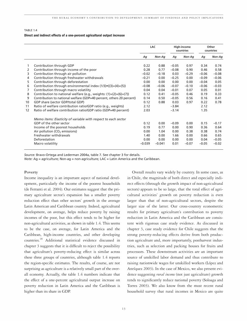
PovertyIncome inequality is an important aspect of national devel-opment, particularly the income of the poorest households(de Ferranti et al. 2004). Our estimates suggest that the pri-mary agriculture sector’s expansion has a smaller povertyreduction effect than other sectors’ growth in the averageLatin American and Caribbean country. Indeed, agriculturaldevelopment, on average, helps reduce poverty by raisingincomes of the poor, but this effect tends to be higher fornon-agricultural activities, as shown in table 1.4. This seemsto be the case, on average, for Latin America and theCaribbean, high-income countries, and other developingcountries.18 Additional statistical evidence discussed inchapter 3 suggests that it is difficult to reject the possibilitythat agriculture’s poverty-reducing effect is similar acrossthese three groups of countries, although table 1.4 reportsthe region-specific estimates. The results, of course, are notsurprising as agriculture is a relatively small part of the over-all economy. Actually, the table 1.4 numbers indicate thatthe effect of a one-percent agricultural output increase onpoverty reduction in Latin America and the Caribbean ishigher than its share in GDP.

Overall results vary widely by country. In some cases, asin Chile, the magnitude of both direct and especially indi-rect effects (through the growth impact of non-agriculturalsectors) appears to be so large, that the total effect of agri-cultural activities’ growth on poverty reduction is evenlarger than that of non-agricultural sectors, despite thelarger size of the latter. Our cross-country econometricresults for primary agriculture’s contribution to povertyreduction in Latin America and the Caribbean are consis-tent with rigorous case study evidence. As discussed inchapter 3, case study evidence for Chile suggests that thestrong poverty-reducing effects derive from both produc-tion agriculture and, more importantly, postharvest indus-tries, such as selection and packing houses for fruits andprocessors. These downstream activities are an importantsource of unskilled labor demand and thus contribute toraising nationwide wages for unskilled workers (López andAnríquez 2003). In the case of Mexico, we also present evi-dence suggesting rural income (not just agriculture) growthtends to significantly reduce national poverty (Soloaga andTorres 2003). We also know from the most recent ruralhousehold survey that rural incomes in Mexico are quite

13


TABLE 1.4

Direct and indirect effects of a one-percent agricultural output increase

LAC High-income Othercountries countries

Ag Non-Ag Ag Non-Ag Ag Non-Ag

1 Contribution through GDP 0.22 0.88 –0.05 0.97 0.34 0.742 Contribution through income of the poor 0.28 0.77 –0.08 0.90 0.46 0.583 Contribution through air pollution –0.02 –0.18 0.03 –0.29 –0.06 –0.084 Contribution through freshwater withdrawals –0.21 0.00 –0.25 0.00 –0.09 –0.065 Contribution through deforestation 0.00 0.00 0.00 0.00 –0.04 0.056 Contribution through environmental index (1/3)•((3)+(4)+(5)) –0.08 –0.06 –0.07 –0.10 –0.06 –0.037 Contribution through macro volatility 0.04 0.04 –0.01 0.07 0.05 0.018 Contribution to national welfare (e.g., weights: (1)+(2)+(6)+(7)) 0.12 0.41 –0.05 0.46 0.19 0.339 Contribution to national welfare (GDP=40 percent, others 20 percent) 0.14 0.50 –0.05 0.56 0.16 0.41

10 GDP share (sector GDP/total GDP) 0.12 0.88 0.03 0.97 0.22 0.7811 Ratio of welfare contribution ratio/GDP ratio (e.g., weights) 2.12 –3.84 2.12 12 Ratio of welfare contribution ratio/GDP ratio (GDP=40 percent) 2.03 –3.14 1.35

Memo items: Elasticity of variable with respect to each sectorGDP of the other sector 0.12 0.00 –0.09 0.00 0.15 –0.17Income of the poorest households 0.19 0.77 0.00 0.90 0.36 0.64Air pollution (CO2 emissions) 0.00 1.04 0.00 0.38 0.38 0.74Freshwater withdrawals 1.40 0.00 1.66 0.00 0.66 0.65Deforestation 0.00 0.00 0.00 0.00 0.04 –0.05Macro volatility –0.039 –0.041 0.01 –0.07 –0.05 –0.02

Source: Bravo-Ortega and Lederman 2004a, table 7. See chapter 3 for details.Note: Ag = agriculture; Non-ag = non-agriculture; LAC = Latin America and the Caribbean.

diversified. On average, agriculture provides less than 40percent of rural household income, including all farmersand nonfarmers (Taylor, Yuñez-Naude, and Cerón 2004).(For farmers, this percentage would be higher.) Finally, arecent Brazil study by Paes de Barros (2003) also suggeststhat the 1990s agricultural boom by itself did not directlycontribute much to poverty reduction through an increasein unskilled labor demand. Instead, the Brazil case showsthat real farm wage increases were linked more strongly tochanges in job and worker characteristics and householddemographics such as higher levels of schooling and theexperience of farm workers, labor force participation, lowerhousehold size, and significant increases in rural nonfarmemployment.

This finding leads to an important policy question.Beyond farming’s indirect contribution to poverty reductionthrough the sector’s integration with downstream industries(which is where poverty impacts are significant), what shouldgovernments do to make primary agricultural production andrural growth in general more pro-poor? The fact that agricul-tural growth is not pro-poor in many Latin American andCaribbean countries seems related to higher asset and incomeconcentration in agriculture than in other activities, under-provision of public goods in the rural space, and the fact thatagriculture taxation and public expenditure incidence can bemore regressive than in other sectors (see De Ferranti et al.[2004], and the evidence below on rural public expenditures).Thus, policies to make agriculture (and rural development ingeneral) more pro-poor would include those attempting tomake access to rural assets (land, education, infrastructure,and credit) more equitable.

One way to attempt more equitable land access is toimplement so-called market-based land reforms to improvethe dismal Latin American and Caribbean distribution ofland assets and/or improve the functioning of land markets,facilitating rotation of assets, rentals, and other land accessforms. Higher land taxes can have beneficial effects in thisregard. However, the historical record of politically motivatedland reforms has been unsatisfactory (Deininger 2003). Moregenerally, we are cautious about the potential for dramaticallyimproving Latin American and Caribbean agriculture’spoverty-reducing effects because we did not find strong statis-tical differences between these effects in Latin America andthe Caribbean as compared to those of other regions; henceLatin America and the Caribbean’s notoriously unequal landdistribution might not be the only explanation for why theincomes of the poorest households react less to agricultural

growth than to the growth of other economic activities(Bravo-Ortega and Lederman 2005). Moreover, we know thatLatin American and Caribbean agricultural incomes are but asmall share of rural incomes.

Further, evidence suggests that broadening access to justone production asset has limited effects (thus land reformwould need to be integrated with broadening access to edu-cation, technology, and credit). Taxing agricultural land andincomes more effectively and focusing public expenditures infavor of the rural poor (at present, public expenditures inrural areas are highly regressive in most countries [see chap-ter 5]) would be complementary policies to make agricul-tural growth more pro-poor. Still, redistributive policiesshould not be pursued at the expense of providing publicgoods in rural areas that are needed to increase overall agri-cultural productivity and that of off-farm rural activities. Aswe show in this report, agricultural production depends cru-cially on farmers’ access to urban and foreign markets(affected by public infrastructure coverage), credit, and tech-nical knowledge (see chapters 5, 6, and 7).

EnvironmentRegarding the environmental consequences of economicgrowth by sector, our evidence indicates that agriculturalgrowth tends to deplete freshwater reserves (over- and under-ground), while other sectors tend to worsen air pollution.Table 1.4 reports the corresponding estimates of theseeffects, which are discussed in chapter 3. But, we also knowfrom international data that deforestation has been a majorconcern in certain Latin American and Caribbean countries,especially those with large amounts of unexploited forestsand potentially arable land. This is the case, for example, inthe Brazilian Amazon. In these cases, substantial literaturehas documented the role played by different types of agricul-tural activities, especially cattle ranching. In addition, it iswell known that in many countries, the expansion of agricul-tural activities and the price reduction of agro-chemicalshave been associated with soil pollution due to the use of fer-tilizers and other agro-chemicals. However, evidence fromChile suggests that the large expansion in the use of suchinputs in the 1990s was basically due to price reductions,while the production shift in favor of exportables actuallyhad a dampening effect on such a trend. Chapter 3 also dis-cusses these issues.

Overall, our conclusion is that agricultural activities canhave deleterious effects on the environment, but the aggre-gate data does suggest that other economic activities tend

14


to have environmental side-effects that might be signifi-cantly worse than those produced by agriculture. In anycase, the patterns of agricultural expansion, deforestation,and general economic progress can be analyzed more rigor-ously from the regional or territorial development view-point. This approach is further discussed below.

VolatilityAnother important consideration in evaluating agricul-ture’s contribution to national development has to do withits effects on economic uncertainty. In a previous report, weconcluded that this was a major concern for the LatinAmerican and Caribbean population, despite the fact thateconomic uncertainty at the national and household levelsactually declined during the 1990s with respect to the1980s (De Ferranti et al. 2001). However, the policy andscientific literature have not examined the sectoral sourcesof macroeconomic volatility. Chapter 3 examines both themagnitude of the contributions of agriculture and othersectors to macroeconomic volatility (that is, unexpectedmovements in national GDP) and potential determinantsof agriculture’s contribution to this volatility.

As table 1.4 shows, the evidence suggests that in high-income countries, agricultural growth is associated withincrements in macroeconomic volatility that are largerthan those caused by other economic activities. In con-trast, for Latin America and the Caribbean as a whole,macroeconomic volatility does not seem to have a particu-lar sectoral source. On the one hand, this could be due tothe role played by large macroeconomic crises, such asexchange rate and financial crises that affected all sectors,thus overwhelming any contribution that might be ema-nating exclusively from the agricultural sector’s volatility.Chapter 3 contains statistical analysis of agriculture’s con-tribution to Latin American and Caribbean volatility,which explains why there is no simple sectoral pattern tothe contribution of the region’s agriculture to macroeco-nomic volatility. While agricultural diversification tendsto reduce agriculture’s contribution to volatility, at thesame time increasing international trade tends to enhancethe sector’s contribution to economic uncertainty. Fur-thermore, these relationships are made more complex bythe finding that international trade is associated withgreater agricultural diversification, thus indirectly reduc-ing agriculture’s contribution to macroeconomic volatil-ity. In addition, public policies can help reduce thesector’s contribution to economic risk, especially policies

related to financial markets, because financial develop-ment (in particular, credit and insurance) tends to be asso-ciated with greater agricultural diversification. Chapter 7covers the public sector’s role in alleviating credit-marketfailures.

With this evidence, we computed agriculture’s potentialcontribution to a broad measure of development thatincluded its contribution to national GDP per capita, butalso to poverty reduction, environmental quality, and thereduction of macroeconomic risk (see table 1.4). Our calcu-lations and methodology are discussed in chapter 3. Forhigh-income countries, which tend to justify agriculturalprotectionism on various potentially spurious arguments,our evidence indicates that agricultural growth during thepast decades has tended to reduce rather than enhance thewelfare of their citizens. In contrast, primary agriculturalgrowth’s contribution to national Latin American andCaribbean well-being tends to be about twice the size ofprimary agricultural production relative to GDP. In otherwords, while the simplistic accounting of the sector impliesthat a one-percent increase in Latin American andCaribbean agricultural production would be related to a0.12 percent increase in national income, our estimate sug-gests that its contribution to national welfare would becloser to a 0.24 percent increase. This realization can haveimportant consequences for the overall policy framework ofour countries, including tax and public expenditure poli-cies, as discussed further below and subsequently in chapter5. Again, country differences are large and will have signif-icant weight in the definition of national policies.

3. While regional or territorial policies hold promiseto enhance national development, they have notreduced Latin American regional disparities Regional policies’ potential effectiveness for enhancingnational development depends on whether regional or terri-torial characteristics affect the well-being of Latin Americanand Caribbean communities—as opposed to just that ofindividuals—in the targeted regions. For this to be true,regional policies, such as investments in the education ofrural populations, must be capable of influencing the targetpopulations’ wages or employment opportunities beyond thepolicies’ effect on each individual’s educational attainment. Ifnot, such interventions can benefit individuals but not neces-sarily communities as a whole or regional economies in par-ticular. In other words, such policies must create positiveregional externalities.

15


Chapter 4 reviews existing and new empirical evi-dence linking regional or territorial characteristics tocommunity-wide wages and employment opportunities.The evidence is clear: regional policies hold some promisebecause community-wide outcomes affect both the numberof jobs and the wages paid at the regional level. Shapingthe territorial distribution of job quality and quantity invarious Latin American and Caribbean countries are thefollowing regional characteristics: distance to major cities,the adult population’s average level of educational attain-ment, and the availability of arable land or other naturalresources.

The aforementioned chapter discusses new evidenceconcerning regional wage determinants in Brazil. Animportant finding is that distance to Sao Paulo matters forwages, but its importance declined during the economicreform period that began in the early 1990s. Figure 1.5illustrates the empirical evidence. The downward solid linedepicts the relationship between wages and distance to SaoPaulo, whereby workers employed in industries in regionsfar away from this city tended to get paid less than similarworkers in closer locations. The statistical analyses dis-cussed in chapter 4 indicate that after the economicreforms, this negative relationship became less dramatic, as

shown by the rotation of the solid line towards the dottedline. Our estimates suggest the effect of this distancebecame less severe and declined somewhere between 2 and6 percent between 1988 and 1999.

Similar evidence was found for Argentina, Brazil, andMexico regarding the quantity of employment opportuni-ties. That is, after the reforms implemented in these coun-tries, especially the opening to international trade, thehandicap of localities far away from major cities (that is,Buenos Aires in Argentina, Sao Paulo in Brazil, and theFederal District in Mexico) became less severe over time,suggesting that reforms were associated with a process ofgeographic de-concentration of employment opportunities.Nevertheless, distance to major markets still helps deter-mine the regional wage and employment patterns observedin these and other Latin American and Caribbean countries.The relevant points of economic attraction shifted from thelargest national cities to export markets. Thus internationaltrade policy can be an important ingredient in regionaldevelopment policies.

Regional educational outcomes also affect regionalwages and employment. In Brazil, the evidence discussedin chapter 4 indicates that a one-percentage point increasein a state’s share of skilled workers (those with a highschool education or higher) is associated with a 2.5 per-cent increase in regional wages and a 0.12 percentincrease in a state’s employment share, after controllingfor the characteristics of workers and industries. However,we did not find evidence that regional educational out-comes affect regional employment opportunities inArgentina or Mexico.

The existence of arable land and other natural resourcesalso helps attract employment to rural areas. As discussedin chapter 4, empirical evidence suggests that endowmentsof arable land generate employment and raise regionalwages in Brazil, but not necessarily in Argentina or Mex-ico. But mining reserves do attract employment opportuni-ties in Argentina and Mexico. Consequently, naturalresources, including land, should be considered key sectorsfor the development of laggard regions or territories inLatin American and Caribbean countries, but they shouldnot be viewed as a panacea for the development of ruralareas, since the evidence is mixed (probably because areaswith good land, but far away from consumer or export cen-ters, cannot use it in a competitive way). In addition, theremay be other less obvious assets, such as natural beauty andenvironmental assets, that benefit not only local popula-

16


FIGURE 1.5

Geographic distances to major cities relative to wages aftereconomic reforms in Brazil

Source: Authors’ calculations based on econometric evidencefrom Bravo-Ortega and Lederman (2004b). Underlying datacome from Brazil’s PNAD household surveys from 1984–99. Seechapter 4 for details.

Wage-distance gradientbefore reforms

Wage-distance gradientafter reforms

= between2% and 6%

Wage

Distance to major city(e.g., Sao Paulo)

17

FIGURE 1.6

Mexican state GDP per capita relative to the federal district, 1940–2000

1940 1950 1960 1970 1980 1988 1990 1993 1995 20000

1

0.9

0.8

0.7

0.6

0.5

0.4

0.3

0.2

0.1

State GDP per capita/federal district's GDP

ChiapasGuerreroOaxacaNuevo LeonSonoraChihuahua

Sources: Lederman, Maloney, and Serven (2004, chapter 2), based on data from Esquivel and Messmacher (2003).


tions, but also the rest of the Latin American andCaribbean national populations (and beyond Latin Americaand the Caribbean), that could contribute to their conserva-tion and use. These assets should also be considered indesigning public policies that aim to support the develop-ment of poor regions, as we discuss below. However, whilethe fact that regional characteristics affect wages andemployment holds promise for regional development poli-cies (RDPs), it does not necessarily imply that historicalexperiences with RDPs in Latin America and the Caribbeanhave been effective.

There are various types of RDPs that have been tried inLatin America and the Caribbean for some time, rangingfrom fiscal (tax) incentives to promote private investmentin particular regions, to attempts by central governmentsto coordinate a plethora of incentives that various govern-ment levels provide. Chapter 4 reviews the theoretical liter-ature that has provided the rationale for alternativeapproaches to public policies that target development ofpoor regions. In turn, chapter 9 reviews various Latin

American and Caribbean experiences and the EuropeanUnion’s experience.

The fact that most countries are still struggling withnotable inter-regional income and employment disparitiessuggests that RDP experiments in most countries, whichdate back several decades, have not been fully satisfactory.For example, figure 1.6 depicts the long-standing develop-ment gaps that exist between Mexico’s southern states(Chiapas, Guerrero, and Oaxaca) and some northern statesand the Federal District. Figure 1.7 illustrates the case ofinter-regional disparities in Colombia over 35 years; itshows that the relative underdevelopment of the Caribbeanregion has been quite persistent. Similarly, there is con-vincing evidence suggesting that inter-regional economicconvergence in Brazil (Magalhaes et al. 2000) and Chile(Soto and Torche 2002) has been quite slow during the pastfew decades.

Moreover, to our knowledge, there are no rigorous eval-uations of RDPs’ impact. The following paragraphs describesome of the attempted policies.

Fiscal incentivesMost Latin American and Caribbean countries have usedvarious fiscal incentives to promote regional development.In Argentina, most provinces have in place one form ofincentive or another, ranging from tax breaks to productionsubsidies, including establishing export processing zones(EPZs) (see chapter 9). There has been very limited evidencethat supports the use of these types of incentives to promoteregional development. New evidence that Sanguinetti andVolpe (2004) provide, discussed in chapter 4, does suggestthat some provinces in Argentina were able to attract indus-tries through such fiscal incentives during 1974–94. Butthe industries that are attracted by such incentives tend tobe of the “footloose” kind, and we have seen no evidencethat the promotion programs help promote national wel-fare. Rather, it is likely that such special regimes have flour-ished in almost every Argentine province, thus suggestingthat a race to the bottom in fiscal responsibility could be anundesirable side effect of such programs.

Likewise, EPZs and other fiscal incentives such as wagesubsidies and sales subsidies have been important compo-

nents of Chile’s overall policy towards its so-called“Extreme Zones” (Zonas Extremas, ZE, in Spanish). Thesefiscal incentives were complemented by raising the alloca-tion of public investments in the target regions, includingthe provision of public housing. These regions (mainlyregions I, XI, and XII in Chile’s regional coding) continueto be considered of geo-strategic importance for Chile andare located in the extreme north and south of the country,in areas that have been characterized by border disputeswith its neighbors. A recent study by Rojas et al. (2004)shows that the fiscal costs of Chile’s EPZ benefits, includ-ing forgone tax revenues plus public subsidies and expendi-tures, was over $420 million in 2001 alone. This numberimplies a total cost per capita in the ZEs that exceeds $630in 2001 or that such expenditures exceeded 10 percent ofthe national population’s average income; thus these are nottrivial fiscal costs, whereas the policy’s effects have not yetbeen properly evaluated. It is quite likely that the fiscalcosts of tax incentives and subsidies in other countries thataim to help regional development are also quite high, andthey still remain unevaluated.

18


FIGURE 1.7

Regional GDP per capita in Colombia as a share of Bogota’s, 1960–96

1960

1962

1964

1966

1968

1970

1972

1974

1976

1978

1980

1982

1984

1986

1988

1990

1992

1994

1996

0

1

0.9

0.8

0.7

0.6

0.5

0.4

0.3

0.2

0.1

Share of Bogota's GDP per capita

CaribbeanWest CentralNorth CentralSouth Central PacificoNew departments

Source: Authors’ calculations based on official data presented in Bonet (2004).

Key sectors and clustersBeginning in the late 1950s, Brazil focused fiscal incentivesand public investments on developing manufacturingindustries in the northeastern states, hoping that trans-forming the northeast’s productive structure would lead itto overcome its development gap. In a sharp reversal in the1990s, promoting agricultural production by expandingthe agricultural frontier became a key ingredient in thecountry’s regional development strategy.

Magalhaes, Hewings, and Azzoni (2000) provide empir-ical evidence that shows that the pace of inter-regional con-vergence was faster during 1980–95 than during the1970s, although during 1970–95 the pace of convergence(or the rate at which the poor states catch up with the richstates, such as Sao Paulo) was very slow, at about 1 percentper year. In fact, these authors as well as Laurini, Andrade,and Valls (2004) found that Brazil might be experiencing aphenomenon known as “convergence clubs,” wherebynortheast states and municipalities are growing at similarlyslow rates, while at the same time the states in the south-east and central Brazil are converging to development lev-els that are significantly higher. In other words, after a longhistory of public interventions justified by the goal of rais-ing the relative development of Brazil’s northeastern states,the reduction pace of inter-regional disparities hasremained anemic at best.

In recent years, establishing production clusters inspiredby the work of Harvard’s Michael Porter and others hasbeen in vogue in the Andean countries and in CentralAmerica. At this time it is too early to reach a firm conclu-sion about the wisdom of pursuing policies that aim toimprove the production linkages across vertically-integrated industries. One reason why this approach mightnot be as successful as expected is that such productionchains can be fragmented, not only across regions in coun-tries, but also across countries. And this production frag-mentation can be economically efficient. However, ifdomestic production chains are underdeveloped due topoor domestic infrastructure, for example, then the publicsector might have an effective role to play. But this is notthe main focus of the key sectors or production clusters’programs that have been tried in various Latin Americanand Caribbean countries. In fact, public infrastructure andother public goods remain significantly undersupplied inthe Latin American and Caribbean rural sector as discussedbelow and in chapters 5 and 7. There are stronger argu-ments, though, to support “innovation clusters” (for exam-

ple, the joint efforts by complementary or competitiveenterprises to develop R&D and skill formation, whereconsiderable economies of scale and group externalitiesmay be present).19 However, such cases are still rare inLatin America and the Caribbean as compared with otherregions.20

The roles of community organizations, the central government, and subnationalgovernments in regional development policies As mentioned above, there is a major potential role forregional and local community organizations and sub-national governments in identifying regional and local spe-cific opportunities and restrictions (as they have betterknowledge of regional/local conditions) and in channelingand coordinating provision demands for specific publicgoods (as there is normally a need to provide or improveaccess to more than one public good to have a significanteffect on growth and poverty reduction). The CDD experi-ence in northeast Brazil and in other Latin American andCaribbean regions appears to give empirical support to thisconceptual conclusion.

Federal and central governments also have a major roleto play in the design, regulation, and coordination of terri-torial development policies. In fact, in the context of LatinAmerican and Caribbean political and fiscal decentraliza-tion, the central or federal government’s role in the imple-mentation of regional development policies might actuallybe as important or more than in previous times. As dis-cussed in chapter 9, even in the European Union (EU), theEU plays an important role in coordinating the variouscontinental programs that aim to support the developmentof its laggard regions.

As an example, since the 1940s, the Mexican govern-ment’s executive branch has been responsible for coordinat-ing its numerous regional development initiatives. Inrecent years, the Mexican federal government has intensi-fied its interest in promoting development in laggardregions. Recent initiatives include the so-called Puebla-Panama project that was expected to lead to substantialinfrastructure investment in the poorest states of SouthernMexico. Even more recently, the Office of the President ofMexico proposed a novel mechanism for funding regionaldevelopment investments, whereby the funds come fromthe federal and local governments plus other donors(including civil society organizations and private firms),but the federal government is expected to coordinate the

19


resulting investments and the processes through which theinvestment decisions are consulted among all relevant actors.Thus this model is slowly approaching the community-leddevelopment model supported by the federal governmentin a strong coordination role. Mexico’s historical experiencewith the coordination of regional development programs isbriefly described in chapter 9. We believe that this coordi-nation model holds great promise, though it is not a sub-stitute for rigorous impact evaluations of the resultinginvestment projects.

4. Biases in Latin American and Caribbean public policies thwart rural developmentThis report contains an extensive discussion of two types ofbiases that may work against Latin American and Caribbeanrural economies. The first is related to rural policies, whichseem to be excessively focused on the provision of subsidies toagricultural producers rather than on the provision of “publicgoods” to develop rural areas. In this regard, we use the term“public goods” to include both the provision of “pure” publicgoods, such as roads and other transport infrastructure, researchand extension, or clean air, and other public sector interven-tions, such as public education and health or regulation ofcredit markets, that have positive effects on societies above andbeyond their effects on particular families or firms. That is, weinclude here all forms of government interventions that resolvemarket failures and stimulate activities with positive externali-ties or reduce those with negative externalities (such as pollu-tion). We also include targeted antipoverty programs, aspoverty reduction is deemed also to be a public good, beyondits effect on individual beneficiaries. The second type of bias isrelated to national policies, including international trade poli-cies and national public expenditures, in terms of their alloca-tion between rural and urban economic activities.

Biases in rural public expenditures policies As mentioned, important components of rural public goodsare infrastructure, knowledge about production techniquesand seeds, human capital, and investment in the protectionof natural resources and the environment. Chapter 5 con-tains both macroeconomic and microeconomic agriculturalproductivity analyses that indicate that market access andthe quantity and structure of education and infrastructureprovision affect agricultural productivity at the nationaland household (farm) levels (see table 1.5). Chapter 6 fur-ther argues that international evidence indicates dramaticsocial returns to public investment in agricultural R&D,

and the most common Latin American and Caribbeansocial rate of return to R&D agricultural investments isabout 40 percent (see table 1.6).

Likewise, human capital is the main productive asset formost poor people. As a consequence of credit and othermarket failures, however, the poor are not in general able tofully finance investments in human capital (or in new tech-nologies), regardless of how high the rate of return to theseinvestments might be (World Bank 2000). They are largelydependent on the public sector as a financing source forthese investments.21 More generally, rural communitiesface natural and economic barriers that limit their access tocredit; chapter 7 discusses the potential roles that the pub-lic sector can play to improve access to credit and infra-

20


TABLE 1.5

The effect of public goods on agricultural sector productivity

Effect in LAC Effect in the rest of the in the 1990s world during 1960–2000

Illiteracy –0.024 –0.0190.000 0.000

Irrigation 0.120 0.0340.180 0.560

Roads 0.424 –0.2090.000 0.000

Telephone density 0.063 0.0620.140 0.020

Credit to private sector 0.001 –0.0010.150 0.020

Electricity generation 0.027 0.0760.380 0.000

Source: Regressions by Bravo-Ortega and Lederman (2004a,table 6). See chapter 5 for details.Note: Effect of a 1 percent increase of each variable on theaverage annual growth of RNR total factor productivity; p-values of elasticities are listed in italic under each estimate.LAC = Latin America and the Caribbean.

TABLE 1.6

Estimated R&D rates of return to the agricultural sector

No. of Standard estimates Mode Mean deviation

Developed countries 78 20 66 120Developing countries 123 40 59 38

Africa 25 30 46 27East Asia and Pacific 38 45 77 52

Latin America and Caribbean 56 40 52 27

Source: Roseboom 2003.

structure by rural households. Likewise, chapter 8 discussesspecific poverty programs that can help poor rural familiesmaintain their children in school, so that future genera-tions of rural communities can find their way out ofpoverty. Moreover, the rural poor are also highly dependenton natural resources as a subsistence source (Barbier 2004).The rural poor often disproportionately pay for resourcedegradation, and investments to protect natural resourcesand reduce environmental externalities are also a means toalleviate hardships associated with rural poverty.

Inadequate provision of rural public goods contributesto slower growth for agriculture and related rural indus-tries. In general, many of the postharvest rural industrieslinked to agriculture are highly intensive in unskilledlabor, which is the principal resource of the poor, and inmany developing countries the rural sector’s share in theunskilled labor market is sufficiently large to influence sig-nificantly the real wages for unskilled workers at thenational level. A growing rural sector is thus an employ-ment source for unskilled workers, plays a role in raisingwages, and consequently is a source of poverty alleviation,even if most of the action in this regard takes place inpostharvest and off-farm rural activities and not in primaryagricultural activities, as discussed above.

Evidence discussed in chapter 5 suggests that rural com-munities in most Latin American and Caribbean countriessuffer from suboptimal investments in the provision of pub-lic goods such as public education, infrastructure, researchand extension, and environmental protection (see, for exam-

ple, tables 1.7 and 1.8), while at the same time there arelarge and largely inefficient and inequitable governmentexpenditures in private subsidies in favor of specific produc-ers that should be redirected towards the provision of publicgoods. On average, across the nine countries for which datais available, between 1985 and 2000 more than 54 percentof total rural expenditures were for private goods and trans-fers that have no significant externalities and that benefitedmostly medium-size and large producers (see table 1.9).Although the government expenditures level and composi-tion have changed significantly over the period (the share of

21


TABLE 1.7

Urban and rural student language attainment by education level

(percent of all students with satisfactory attainment)

Urban Rural

Country Level I Level II Level III Level I Level II Level III

Argentina 96 79 59 88 62 42Bolivia 87 58 35 77 40 24Brazil 95 82 58 84 62 38Chile 95 79 60 89 63 41Colombia 89 60 36 89 57 33Cuba 100 98 92 100 98 92Dominican Republic 73 44 25 73 39 20Honduras 87 55 29 78 35 17Mexico 89 64 43 82 48 30Paraguay 90 67 44 81 51 32Peru 86 57 34 71 30 13Venezuela, R.B. de 88 60 38 84 58 39

Source: OREALC/UNESCO 2001.

TABLE 1.8

Latin American and Caribbean differentials in access to safe water

1990 2000

Rural Urban Rural Urban

Honduras 78 89 81 95Jamaica 87 98 85 98Mexico 52 90 69 95Nicaragua 44 93 59 91Panama . . . . 79 99Paraguay 46 80 59 93Uruguay . . . . 93 98Venezuela, R.B. de . . . . 70 85

Latin America and the Caribbean 57.82 92.41 65.36 93.95

Source: World Health Organization and UNICEF, cited in WorldBank 2003a.

22


private subsidies declined notably for most countries22 andfor the five-year period, 1985–90, across all countries fellfrom 60 percent to 44 percent for 1995–2000), remainingshares are still excessively high.

Statistical evidence that López (2004) provided for thisreport indicates that this poor allocation of rural expendi-tures has severe consequences. For example, it suggests thatan increase of one percentage point in the share of ruralpublic expenditures dedicated to the provision of publicgoods in Latin American and Caribbean countries is associ-ated with a per person agricultural production growth ofabout 0.23 percent. In contrast, increasing total ruralexpenditures by one percent without changing its composi-tion raises agricultural incomes by only 0.06 percent. Thusthe restructuring of public rural expenditures must takeprecedence over increasing total rural expenditures,although our estimates suggest that, once this is done,national development in the future will benefit from over-all rural expenditure increases, as they will be mostly dedi-cated to the provision of rural public goods. Indeed, wefound evidence of an overall pro-urban bias in the alloca-tion of total public expenditures, as shown below.

Remaining antirural biases in national (and international) public policiesOne of the most sensitive issues that we tackle in this reportconcerns the structure of public policies in terms of theirpotential effects on rural and urban economic activities. Animportant set of policies concerns international trade barri-ers, which can have consequences for the allocation of pro-

ductive resources across agricultural and non-agriculturalactivities. A second set of issues concerns the global alloca-tion of public expenditures between rural and urban areas.

Agricultural trade and the structure of import tariffs Chapter 6 provides a detailed discussion of the potentialeffects that agricultural protectionism in OECD countrieshas on various Latin American and Caribbean countries asboth as importers and exporters, especially import restric-tions and subsidies offered to agricultural producers. TheLatin American and Caribbean region is very heteroge-neous; while agricultural exports are a significant foreignexchange source for most countries, a high proportion ofcountries are net food importers. The existing evidencesuggests that the impact of OECD agricultural tradereforms would have different effects on Latin American andCaribbean countries depending on their individual tradepatterns. Overall, OECD import barriers seem to be moreimportant than OECD domestic subsidies for Latin Ameri-can and Caribbean agricultural exports. The removal ofrich-country protectionist measures can also have differenteffects on national economies, depending on whether acountry is a net exporter or net importer of the protectedcommodities. As chapter 6 shows, 15 of 22 Latin Americanand Caribbean countries examined are net food importers;these import prices will rise when OECD farm-sector pro-tection is reduced (see table 1.10).

Thus it is difficult to generalize about the potentialeffects that global trade reforms or regional trade agree-ments might have on the Latin American and Caribbean

TABLE 1.9

Composition of rural public expenditures

Subsidies as Public Public goods as Total Subsidies % of total goods % of total expenditures

Countries ($ millions) expenditure ($ millions) expenditure ($ millions)

Costa Rica 41.6 47.4 46.1 52.6 87.7Dominican Republic 174.6 65.4 92.2 34.6 266.8Ecuador 89.8 67.3 43.61 32.7 133.4Honduras 3.3 10.8 27.6 89.2 31.0Panama 82.9 80.8 19.6 19.2 102.5Paraguay 106.5 86.5 16.6 13.5 123.1Peru 197.3 55.0 161.4 45.0 358.7Uruguay 7.7 19.1 32.42 80.9 40.1Venezuela, R.B. de 283.8 54.2 239.9 45.8 523.8

Source: López (2004) based on data supplied by FAO, Regional Office for Latin America andthe Caribbean, Santiago, Chile.

23


TABLE 1.10

Latin American and Caribbean countries are net agricultural

exporters, but many are net food importers

All agricultural Food exports exports and and imports imports

EX/IM EX/IM

South AmericaArgentina 24.2 12.5Bolivia 1.1 1.7Brazil 2.8 4.2Chile 0.6 2.7Colombia 0.5 1.9Ecuador 0.4 3.4Paraguay 2.2 1.7Peru 0.1 0.7Uruguay 6.5 2.6Venezuela, R.B. de 0.1 0.2Total South America 2.4 3.2

Central America and MexicoCosta Rica 0.9 3.3El Salvador 0.4 0.7Guatemala 0.9 1.8Honduras 0.2 1.3Mexico 0.2 0.7Nicaragua 1 1.4Panama 0.3 0.8Total Central America and Mexico 0.3 0.9

Latin America and the Caribbean 1.1 1.8

Source: Authors’ calculations based on FAO data.

region’s national economies. Countries such as Argentinaand Brazil would undoubtedly gain from the removal ofworldwide agricultural trade barriers and domestic subsi-dies in OECD countries. But many countries that are netimporters of protected or subsidized products might expe-rience deteriorations in their terms of trade if prices of someimported agricultural commodities rise as a consequence oftrade reforms. Thus, we argue that, given the enormouspotential contribution to national growth of agriculturalexports, trade negotiations should focus more on achievingbroader market access and reducing those domestic subsi-dies that reduce or impede market access of potentiallycompetitive sectors, while at the same time “buying time”and putting in place programs to support the restructuringof small domestic producers in importing sectors thatwould not be competitive even with a reduction of OECDdomestic subsidies (see below).

Latin American and Caribbean policy makers canaddress an important source of sectoral biases in trade poli-

cies directly—the structure of Latin American andCaribbean trade barriers. Chapter 7 analyzes one protectionmeasure, namely the tariff schedules that countries reportto the World Trade Organization (WTO). Contrary to thewidespread image of an unprotected, competitive, export-oriented agriculture in Latin America, MFN tariffs for agri-cultural and food product imports are relatively high formany Latin American and Caribbean countries. The aver-age tariff level for livestock is 17 percent, for crops 12 per-cent, and for textiles 18 percent (see table 1.11). Mexicohas the highest MFN tariffs for agriculture and food prod-ucts, though they have been reduced under bilateral agree-ments with its largest trading partners; next is Peru. Chilehas the lowest tariffs, and as of 2004, its uniform MFN tar-iff is 6 percent, but it maintains special price-settingregimes for three agricultural commodities. Overall, cropsand the wood products sectors are protected comparablyless than livestock. Processed food products also receivehigher protection, demonstrating the widespread phenom-enon of tariff escalation in developed and developing coun-tries. Of the various sectors, textiles are generally mostprotected, and industrial protection is similar to livestockand processed foods, but higher than crops.

Except for Bolivia and Chile, where uniform (and low) tar-iffs are the rule, the tariff data indicates that there are surpris-ingly high proportions of tariff peaks—that is, the number ofproducts that face abnormally high import tariffs—in allproduct categories; in many cases, more than 70 percent of allcategory lines are affected. The highest proportion of tariffpeaks is found in Argentina, Brazil, Colombia, and RepúblicaBolivariana de Venezuela. As in the case of average tariffs byproduct category, livestock and food products generally have agreater number of peaks as a proportion of tariff lines thancrops do. Nevertheless, the proportion of tariff peaks for cropsis notably high for Colombia, Guatemala, Honduras, Mexico,Peru, and República Bolivariana de Venezuela. Conspicu-ously, the six MERCOSUR (Southern Cone Common Mar-ket) countries (including associate members) have no croptariff peaks, although for forestry, livestock, and processedfood, there is a very high incidence of tariff peaks for thisgroup of countries (except Bolivia and Chile). AlthoughMERCOSUR has uniformly low crop protection, these com-modities are protected by tariffs that exceed 15 percent in atleast 45 percent of tariff lines in that category in the otherLatin American and Caribbean countries (see table 1.12).Coupled with the significant reductions that have occurred inmost countries in tariff and nontariff protection for manufac-

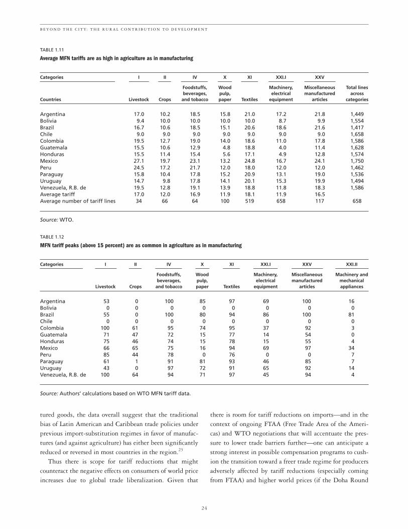
24


TABLE 1.11

Average MFN tariffs are as high in agriculture as in manufacturing

Categories I II IV X XI XXI.I XXV

Foodstuffs, Wood Machinery, Miscellaneous Total lines beverages, pulp, electrical manufactured across

Countries Livestock Crops and tobacco paper Textiles equipment articles categories

Argentina 17.0 10.2 18.5 15.8 21.0 17.2 21.8 1,449Bolivia 9.4 10.0 10.0 10.0 10.0 8.7 9.9 1,554Brazil 16.7 10.6 18.5 15.1 20.6 18.6 21.6 1,417Chile 9.0 9.0 9.0 9.0 9.0 9.0 9.0 1,658Colombia 19.5 12.7 19.0 14.0 18.6 11.0 17.8 1,586Guatemala 15.5 10.6 12.9 4.8 18.8 4.0 11.4 1,628Honduras 15.5 11.4 15.4 5.6 17.1 4.9 12.8 1,574Mexico 27.1 19.7 23.1 13.2 24.8 16.7 24.1 1,750Peru 24.5 17.2 21.7 12.0 18.0 12.0 12.0 1,462Paraguay 15.8 10.4 17.8 15.2 20.9 13.1 19.0 1,536Uruguay 14.7 9.8 17.8 14.1 20.1 15.3 19.9 1,494Venezuela, R.B. de 19.5 12.8 19.1 13.9 18.8 11.8 18.3 1,586Average tariff 17.0 12.0 16.9 11.9 18.1 11.9 16.5Average number of tariff lines 34 66 64 100 519 658 117 658

Source: WTO.

TABLE 1.12

MFN tariff peaks (above 15 percent) are as common in agriculture as in manufacturing

Categories I II IV X XI XXI.I XXV XXI.II

Foodstuffs, Wood Machinery, Miscellaneous Machinery and beverages, pulp, electrical manufactured mechanical

Livestock Crops and tobacco paper Textiles equipment articles appliances

Argentina 53 0 100 85 97 69 100 16Bolivia 0 0 0 0 0 0 0 0Brazil 55 0 100 80 94 86 100 81Chile 0 0 0 0 0 0 0 0Colombia 100 61 95 74 95 37 92 3Guatemala 71 47 72 15 77 14 54 0Honduras 75 46 74 15 78 15 55 4Mexico 66 65 75 16 94 69 97 34Peru 85 44 78 0 76 0 0 7Paraguay 61 1 91 81 93 46 85 7Uruguay 43 0 97 72 91 65 92 14Venezuela, R.B. de 100 64 94 71 97 45 94 4

Source: Authors’ calculations based on WTO MFN tariff data.

tured goods, the data overall suggest that the traditionalbias of Latin American and Caribbean trade policies underprevious import-substitution regimes in favor of manufac-tures (and against agriculture) has either been significantlyreduced or reversed in most countries in the region.23

Thus there is scope for tariff reductions that mightcounteract the negative effects on consumers of world priceincreases due to global trade liberalization. Given that

there is room for tariff reductions on imports—and in thecontext of ongoing FTAA (Free Trade Area of the Ameri-cas) and WTO negotiations that will accentuate the pres-sure to lower trade barriers further—one can anticipate astrong interest in possible compensation programs to cush-ion the transition toward a freer trade regime for producersadversely affected by tariff reductions (especially comingfrom FTAA) and higher world prices (if the Doha Round

TABLE 1.13

Public rural expenditures compared with agriculture/GDP ratios

Ratio of rural expenditure/total expenditureCountries to agricultural GDP/total GDP

Chile 1.26Costa Rica 0.52Dominican Republic 2.32Ecuador 0.02Honduras 1.61Panama 1.23Paraguay 0.51Peru 0.67Uruguay 0.02Venezuela, R.B. de 1.37

Source: Authors’ calculations based on data supplied by FAO,regional office for Latin America and the Caribbean, Santiago,Chile, and World Bank data.

25


succeeds). Chapter 8 addresses possible types of compensa-tion schemes that might provide such a cushion. Theseshould ideally combine temporary income transfers (à laProcampo in Mexico) with technical support to small farm-ers in these sectors to facilitate restructuring, the adoptionof more productive technologies, practices, and varieties, ora shift to new activities, and improving their access tocredit and consumption markets.

The structure of national public expenditures After the rural expenditure restructuring proposed above,the efficiency of Latin American and Caribbean ruralexpenditures could improve and thus justify a further real-location of total public expenditures from urban to ruralareas. This conclusion is derived from the observation thatnational welfare is best served by an allocation of publicexpenditures that is driven by each sector’s relative contri-butions to national development, as long as the efficiency ofboth types of expenditures is about equal.

As of 2000, the evidence discussed in chapter 5 indi-cates that most Latin American and Caribbean countries forwhich we obtained rural and total expenditure data hadallocated about half the amount to rural areas that would bejustified by agriculture’s contribution to national develop-ment (see table 1.13). In fact, out of the 10 countries stud-ied in chapter 5, only the Dominican Republic had a ratioof rural-to-total expenditures that was close to twice itsagricultural GDP share.

However, the Dominican Republic is one of the coun-tries with the worst distribution of rural expenditures inLatin America and the Caribbean, as over 45 percent ofrural expenditures were destined for the provision of pri-vate subsidies during 1995–2000. Ecuador and Paraguaydestined over 70 percent of their rural expenditures to sub-sidies during the same period, and thus were the worst per-formers out of the 10 Latin American and Caribbeancountries examined in chapter 5. As a result, we cannotoveremphasize the need to pursue a sequence of publicexpenditure reforms, whereby the first step is to improvethe structure of rural expenditures; the next step shouldinclude a broader reallocation of public expenditures fromurban to rural areas. Although there is a bias against ruralareas in the provision of most public goods (education,infrastructure, and R&D), a simple reallocation of totalpublic expenditures in favor of rural areas under presentbudgetary trends would not be efficient because a highshare of rural public expenditures are subsidies to private

groups, which are neither efficient nor equitable. Thisproblem of the inefficient public expenditures structure,which would undermine the benefits of any shift in publicspending toward rural areas, is explained by both politicaleconomy and institutional factors, as discussed in the firstfinding (p. 7).

Policies for poor regions require a broad definition of “assets”Many laggard rural regions in Latin American andCaribbean countries are poor even though they have naturalassets that, in theory, should enable them to overcomepoverty. The clearest example of such assets is the availabil-ity of arable land and other natural resources, such as forestsand mineral riches. These assets are important for regionaldevelopment because they can attract private investmentand thus lead to a process of social and economic develop-ment. However, this does not always occur because comple-mentary production factors, including labor and capital,might seek higher returns in other economic activitieslocated in cities or other regions. A better allocation ofinvestments in public goods between urban and rural areasand between major cities and laggard regions might changethe balance for some areas, but most probably not for all.

Some laggard regions, however, can also have other lessvisible assets that provide significant welfare benefits forthe national population, not just for the local residents. Forexample, some rural regions contain bodies of water thatprovide natural processes through which water is cleansed.

They also have natural forests that help clean the air. Thevalue of these assets and their contributions to the well-being of society as a whole is admittedly difficult to calcu-late, and chapter 8 in this report covers the existingliterature on these environmental services. Beyond thechallenge of measuring these contributions to develop-ment, it is nevertheless quite obvious to us that thenational and perhaps even the international communityshould pay nontrivial amounts for these services. If a seri-ous effort is undertaken to pay for these valuable services,then the resulting resources can be used to make the neces-sary public investments to safeguard these assets and toprovide other public goods that might help the emergenceof agricultural or non-agricultural activities in laggardregions. Thus chapter 8 also covers issues related to envi-ronmental services and rural tourism, a sector that canflourish only if environmental assets are safeguarded. Thereport discusses the public sector’s role in stimulating thesetypes of industries, although we acknowledge that neitherthis, nor a better allocation of public goods, might be aviable alternative for many people in some of the poorestregions in Latin American and Caribbean countries. Inthese cases, there will be few alternatives to improvinghuman capital to facilitate labor mobility in sectors orregions (domestic or international migration), as wagestend to be higher in nonfarm activities, but many of theserequire higher educational levels. Both off-farm employ-ment and migration (and associated remittances) have beenfound to be an important strategy of poor households toincrease their income levels and diversify risk.

1.3 Conclusions: The need for institutional reformsImplementing the suggested rural policy reforms can bedifficult. In particular, there might be political forces thathave shaped the structure of rural policies, including thestructure of public rural expenditures, through the courseof history. Thus we acknowledge that certain institutionalreforms and political activism might be needed to enablethe restructuring of rural public policies. For example, theministries of education, health, and public works usuallyundertake the allocation of public investments in the pro-vision of public goods in the corresponding sectors of edu-cation, health, and infrastructure. These ministries arenormally more responsive to the needs and pressures of con-centrated and organized urban voters and interests, includ-ing those of service providers. Existing ministries ofagriculture are about the only voice with a pro-rural bias in

governments, but they have virtually no voice in govern-ment deliberations about how and where to spend scarcepublic funds for these services. Thus it is not surprisingthat in many Latin American and Caribbean countries, theministries of agriculture have become a marginal ministrywith the main role of representing the interests of influen-tial agricultural producers, especially those in noncompeti-tive sectors. The overall process results in a highly-skewedstructure of public expenditures in rural areas, with signif-icant underprovision of public goods and huge transfersand subsidies that favor mostly large producers, especiallyin noncompetitive sectors, thus reducing the effectivenessand equity of rural public expenditures. We must thinkhard about how to reform public institutions and the polit-ical process so that rural communities get a seat at the tablewhen the provision of public goods for rural and urbanareas is decided on and avoid the capture of large chunks ofpublic expenditures (and policies) by large agriculturalproducers in specific sectors.

As mentioned above, fiscal and political decentralizationhave taken place in the context of wide inter-regional dis-parities, both in terms of social outcomes (education,health, and poverty) as well as in terms of purely economicoutcomes. In theory, however, increasing local oversightover government functions can also improve the quality ofpublic services, as long as local interest groups do not cap-ture local governments. For the same reason, we need tosupport community-led development strategies that involvelocal peasant and other communities in the decision-making process. As mentioned before, there is strong evi-dence in favor of the potential contribution of welldesigned and implemented “territorially-based” rural orregional development policies. Both community organiza-tions and local and regional governments have a central rolein identifying opportunities and bottlenecks and coordi-nating demand and supply of public goods. However, cen-tral governments must also strengthen their roles asregional development program coordinators, as theyremain the crucial actors in the provision of key publicgoods (such as R&D and inter-regional infrastructure) andas territorial development and policies have inter-regionalexternalities. Few other institutions are better positioned toensure that overall regional public investments are focusedon the provision of public goods that can benefit not onlylocal communities, but also the nation as a whole.

In the case of many poor and remote areas, where agricul-tural (that is, forestry, fishing, and mining) activities may

26


not be competitive even under an improved spatial alloca-tion of public goods and sectoral policies, we must find away for societies to pay for the delivery of environmentalservices (such as conservation, biological research, and ruraltourism) from which all, present and/or future citizens, willbenefit. And we must also facilitate the provision of humancapital to all (including through targeted conditionalincome transfers to the rural poor) that will allow morelabor mobility, across sectors or territories, for the poor andwill give income support to remaining poor families.

In sum, this report argues that agricultural developmentand territorial development, which includes other ruralactivities, are not only compatible, but also need to bestrengthened through smart public-sector interventionsthat focus on the provision of public goods in the ruralspace. This approach will allow rural families and commu-nities to make their own decisions about which activities topursue and how to pursue them as long as the public sectorand the international community provide opportunities forthem to overcome poverty.

This report also demonstrates that rural development isin the national interest of most Latin American andCaribbean countries. At a minimum, we hope to provokenational and international dialogues about how we canwork together with governments and civil society toenhance the rural contribution to Latin American andCaribbean development. And we have a social responsibil-ity to go beyond the traditional focus on growth and con-sider more the consequences of public actions for povertyand the environment.

1.4 Report organization The report is organized in two parts: the first covers analyt-ical issues about the rural sector’s size and contribution andthe potential effects of territorial development policies; thesecond centers on policy issues.

Part I has three chapters. Chapter 2 discusses the “real”size of the Latin American and Caribbean rural sector, bothfrom a sectoral (activity-based) and a territorial (population-based) viewpoint. Chapter 3 estimates the contribution ofLatin American and Caribbean agricultural growth tonational economic growth, poverty reduction, macroeco-nomic volatility, environmental degradation, and welfare.Chapter 4 discusses potential effects of territorial(“regional”) development policies.

Part II has five chapters. Chapter 5 identifies the deter-minants of agricultural productivity and growth and esti-

mates the effects of the composition of Latin Americanand Caribbean rural public expenditures. Chapter 6 dealswith three crucial determinants of agricultural productiv-ity and growth: trade, research and extension, and landpolicies. Chapter 7 covers two important determinants ofboth agricultural and other rural activities’ productivityand growth: rural infrastructure and rural finance. Chap-ter 8 deals with complementary policies related to envi-ronmental services, rural tourism, and income supportschemes for the poor and for small farmers in “sensitive”sectors during trade liberalization. Finally, chapter 9 dis-cusses different approaches to territorial developmentpolicies, summarizes Latin American and Caribbean expe-riences with such policies, and extracts some generallessons going forward.

Notes1. “Agricultural activities” in this report include crops, live-

stock, forestry, and fisheries. This commodity-agriculture sector isreferred to as the “Rural-Natural-Resource” (RNR) sector in chap-ters 2, 3, and 4. “Expanded” agriculture includes RNR productionplus the value added by the downstream industries, such as foodand processed products that use domestically-produced RNR prod-ucts. This definition of the expanded agricultural sector should bedistinguished from the augmented agricultural sector that IICA(2004) and other sources use, which is simply the sum of RNRgross domestic product (GDP) plus the GDP of all of the down-stream industries, not just the portion that relies on domestically-produced RNR products. Some statistical analyses presented inchapter 3 do use the sum of the RNR and downstream-industryGDPs.

2. Defined as cities of 100,000 inhabitants or more.3. National welfare defined as a weighted average of growth,

poverty reduction, environmental, and volatility effects.4. Similar results are obtained for other developing countries

outside the region, but not for developed countries. In the latter case,the growth of agricultural activities appears to detract from growthand welfare in the rest of the economy, probably as a consequence ofhigher labor scarcity and excessive protection that these activitiestypically receive in OECD countries.

5. Measured as the ratio to total public expenditures/ratio ofagriculture to GDP.

6. See, in particular, De Ferranti et al. (2002). 7. Referred to as the RNR sector in chapters 2, 3, and 4.8. See, for example, the evidence presented by Lederman, Mal-

oney, and Servén (2004). 9. Lederman, Maloney, and Servén 2004.

10. In human capital in the case of Oportunidades.11. We estimate that the marginal income elasticity of land is

close to zero.12. De Janvry 2004. 13. See Burki, Perry, and Dillinger (1999).

27


14. The nine Latin American and Caribbean countries included inIICA (2004) are Argentina, Brazil, Chile, Colombia, Costa Rica,Mexico, Peru, Uruguay, and República Bolivariana de Venezuela.

15. It is also noteworthy that IICA (2004) reports that GDPshares of primary agriculture plus food processing industries rangedfrom 20.5 percent in R.B. de Venezuela to 34.8 percent in Uruguayin 1997. This study also reports higher numbers for the GDP share ofprimary agriculture than our numbers, but both sets of calculationsinclude commodity agriculture, plus forestry and fisheries.

16. It may be argued, though, that such criteria (specially the dis-tance to a large urban center) should be adjusted by the country’s rel-ative size.

17. It is possible that the magnitude of this effect has changedover time due to trade liberalization and globalization (which tend toproduce higher fragmentation of production among countries) andagriculture modernization. These two effects act in opposite direc-tions, and it is difficult to establish robust econometric estimates ofnet trends.

18. The econometric analysis underlying these estimates consid-ered each country as a separate and equal policy experiment; theregressions were not weighted by each country’s population. Thusthese results are not necessarily inconsistent with the fact that a largeportion of the world’s poor live in rural areas when one counts therural poor in China and India.

19. See, for example, De Ferranti et al. (2003). 20. Chile being a probable exception, with successful government

R&D support of the salmon industry and other cases.21. Public support of human capital formation for the poor can

either be in the form of the direct government provision of educationand health care services, or in the form of vouchers and other transfersthat allow access to privately provided services.

22. Only Paraguay experienced an increase in the share of subsi-dies between the two periods.

23. There is evidence that in some countries such a bias againstagriculture may have never existed (see Kalmanovitz [2004] forColombia).

28


PART I

The Rural Contribution to Development: Analytical Issues

31

CHAPTER 2

How Do We Define the Rural Sector?

TO UNDERSTAND THE RURAL ECONOMY’S NATIONAL DEVELOPMENT ROLE, THIS CHAPTER

presents an overview of particularly relevant areas of the Latin American and Caribbean ruraleconomy. The rural economy is more than agriculture; it includes forestry and fisheries pro-duction and other economic activities that take place in nonurban areas. There are at leastthree ways of describing the rural economy: a sectoral approach, which emphasizes the sector’s

contribution to national GDP; a household income approach that includes farm and nonfarm activities; anda territorial approach that examines rural space more generally, in terms of population density and distancefrom cities.

From a sectoral perspective, as a country develops one expects increasing intersectoral integration due toforward and backward linkages between the rural natural resources (RNR) sector and the rest of the economy.What is the magnitude of the links between RNR production and the rest of the economy? What is itsshare of international trade? If there are substantial links, “agriculture” developments would influencedevelopments in related sectors and thus have a higher impact on the overall economy than is captured byagriculture’s GDP statistics.

breakpoint based on a set of characteristics. The changesfrom very remote towns to the largest city are often grad-ual. But in policy formation there have to be some criteriaor thresholds to guide administration. In terms of the eco-nomic efficiency of public investments, one set of criticalelements that could distinguish rural areas from urban arethe cost gradients of providing social services and infra-structure, which depend on population densities and dis-tances. What is referred to as “rural” population in theLatin American and Caribbean region reflects each coun-try’s official statistics, with country-specific definitionsand criteria. Criteria vary by country and are chosen with-out reference to an international standard.

This chapter presents an approach to defining rural pop-ulations based on density and distance from urban centers,which allows international comparisons and could providethe basis for the adoption of a common set of criteria for

Looking beyond the perspective of sectoral production,rural areas comprise a diversity of activities beyond agricul-tural production. Taking a purely sectoral perspective wouldbe incomplete, because a high proportion of households inrural areas have income sources that are not directly agricul-ture-related. As we will see below, there is a large amount ofrural non-agricultural employment and income in theregion, based on official definitions of rural populations.

This is significant, because rural nonfarm employmentrepresents an increasingly important part of the rural econ-omy in terms of income, employment, poverty alleviation,and economic development.

From a social perspective, what criteria would permitthe separation of rural and urban spaces? What is typicallyconsidered rural space encompasses activities and personslocated in low population density areas, usually distantfrom urban centers. But there is no natural dividing line or

defining rural areas in the Latin American and Caribbeanregion. And the evidence below will show that the regiontends to underestimate the population size living in areasthat can be reasonably called rural. Clarifying what is ruralwill grow increasingly more relevant to the evaluation ofrural area assistance and, more important, in the promotionof greater decentralization and territorial development.

The overview presented below is an attempt to provide adescriptive profile across countries, capturing the notableheterogeneity of the region’s rural economies. It lays outthe basic facts regarding the rural economy’s size and struc-ture, based on various indicators. These are: the GDP shareof RNR production to national GDP; RNR trade’s impor-tance and composition; rural income sources and povertyincidence; and a presentation of an approach to definingrural areas based on the number of persons living in low-density and remote areas.

2.1 How big is the RNR sector? The direct contributions of the primary sector—namely,rural natural resources, or often “agriculture”—to thenational economy are often depicted in terms of its GDPparticipation, its foreign exchange earnings, and its role insupplying savings and labor to other sectors.1 These formthe traditional roles of the RNR sector (crops, livestock,forestry, and usually fisheries) described decades ago, forexample, in Johnston and Mellor (1961). For Latin Amer-ica, the post-WWII development literature contained pes-simistic assessments of the sector’s potential forproductivity and export growth. In addition, the sector waspresumed to be unresponsive to incentives (for example,Prebisch 1959), with a perceived absence of linkages toother sectors (Hirschman 1958). This set of stylized factsled to the conclusion that spurring agricultural growth wasa low priority in the search for policies that would stimu-late national economic development (Lewis 1954).

Following Schultz (1964) and others, developmenteconomists changed their attitudes toward agriculture’sefficiency and growth potential. Econometric analysis sug-gested that agriculture in developing countries was asresponsive as in industrial countries and that agriculturewas capable of productivity growth and responsive to tech-nological change. With respect to the links between agri-culture and the rest of the national economy, the evidencedemonstrated that the farm sector could have significantmultiplier effects and therefore that agricultural growthcould be propagated to other economic sectors (Adelman

32


and Morris 1973; Mellor 1976; Bell and Hazell 1980;Hazell and Haggblade 1990; Delgado et al. 1998).2 In partbecause most of the above research focused on near-subsis-tence agriculture (primarily in South Asia), the findingsconcerned primarily the importance of linkages throughfarm-production generated household consumption, ratherthan through inter-industry effects.

More broadly, as countries develop and agriculture mod-ernizes, one expects an increasing intersectoral integrationalong the supply chain, between industries that supply theRNR sector with inputs and equipment, and the RNR sec-tors that supply processing industries and the marketing anddistribution sector. RNR sector development will depend ondevelopments in these other sectors, and their developmentwill depend to some extent on what happens in agriculture,forestry, and fisheries. The changing nature of the relation-ships between sectors is manifested by new technologies andnew financial and business interactions. And the depth ofintegration will be conditioned by the economy’s openness totrade, sources of new equipment and technologies, inputs,and the destination of new products. Relationships betweensectors have consequences for restructuring agriculture andthe rural sector more generally, in terms of the distributionof farm sizes, the crop and product mix, and the concentra-tion of agro-processing and retail trade.

An important question, therefore, especially for middle-income countries in Latin America (where the RNR sectortypically represents a small GDP3 share), regards the mag-nitude of the integration of agriculture, forestry, and fish-eries with other sectors relative to the primary sector’s size.Are linkages between the RNR sector and the nationaleconomy relevant for development strategy? The extent ofthe sector’s links to the rest of the economy determines itsreal size and importance to the overall economy.

2.2 RNR sector composition based on national accountsWhat is the size of the agriculture, forestry, and fisheriessector’s direct contribution to national output? The share ofnational GDP attributable to a broadly-defined RNR pri-mary sector—officially called “agriculture”—varies acrosscountries, tending to fall with the degree of a country’s eco-nomic development as measured by GDP per capita (seetable 2.1). Across the region, the range of GDP sharesattributable to the RNR sector varies between 1.5 percentfor Trinidad and Tobago to 30.8 percent for Guyana. Overtime, the RNR GDP share has declined for all countries,

and in some cases steeply, as in Colombia, Ecuador, Mexico,and Uruguay. For the region as a whole, the share of RNRin GDP was 7 percent in 2002 compared with 8.8 percentin 1990.

In terms of RNR sector composition, although disaggre-gated data is not available for all countries, table 2.2 showsthat across Latin America, crop production accounts for about60 percent of the sector’s GDP, while livestock production

accounts for between a quarter and slightly more than one-third. Uruguay is an exception, having a notably large live-stock subsector (70 percent of RNR GDP). Forestry isrelatively large in a few countries—Chile, Ecuador, Paraguay,and Uruguay—and has generally grown over the last decade.Fisheries represent an important share of the RNR sector’sGDP in a few countries along the Pacific coast: Chile (21 per-cent), Ecuador (13 percent), and Peru (9 percent).

33

H O W D O W E D E F I N E T H E R U R A L S E C T O R ?

TABLE 2.1

Evolution of agriculture GDP in the Latin American and Caribbean region, 1990–2002

Country 1990 1991 1992 1993 1994 1995 1996 1997 1998 1999 2000 2001 2002 2003

Antigua and Barbuda 4.2 4.2 4.2 4.1 3.7 3.9 3.9 4.1 4.0 3.9 3.9 3.8 3.8 —Argentina 8.1 6.7 6.0 5.6 5.5 5.8 6.1 5.7 5.7 4.8 5.1 4.9 10.8 11.1Barbados 7.4 7.4 7.1 6.8 6.5 6.3 7.2 7.0 5.8 6.2 6.2 6.0 5.8 —Belize 20.0 18.4 17.8 16.9 16.9 18.0 17.9 17.5 16.9 17.5 17.2 15.4 15.1 —Bolivia 16.7 17.1 16.0 16.3 17.1 16.9 16.4 17.2 14.7 15.1 14.9 15.2 14.6 14.6Brazil 8.1 7.8 7.7 7.6 9.9 9.0 8.3 7.9 8.4 7.2 7.2 6.1 6.0 —Chile 8.7 9.9 9.9 9.2 9.4 9.2 9.0 8.4 8.5 8.4 8.5 8.8 8.8 8.8Colombia 16.7 17.4 15.8 13.9 16.1 15.3 13.8 13.7 14.3 14.0 14.0 14.0 13.9 14.0Costa Rica 17.9 13.4 13.3 13.0 13.4 13.7 12.8 13.0 12.8 10.5 9.4 8.6 8.4 8.3Cuba — — — — — 6.0 6.8 6.7 6.2 6.4 6.7 — — —Dominica 25.0 23.8 22.4 21.5 21.7 18.9 19.9 19.4 18.8 18.7 18.1 17.7 18.6 —Dominican Republic 13.4 13.9 13.6 13.3 12.5 12.6 12.8 12.2 11.5 11.4 11.2 11.4 11.8 10.6Ecuador 13.3 14.4 12.8 19.7 16.8 16.7 15.6 15.8 13.8 11.7 10.6 9.0 9.0 9.1El Salvador 17.1 17.1 14.2 14.0 14.0 13.4 13.0 13.4 12.0 10.5 9.8 9.4 8.7 9.4Grenada 13.4 13.1 11.2 10.6 10.1 10.1 8.6 8.4 7.9 8.1 7.8 7.8 7.5 —Guatemala 25.9 25.7 25.3 24.9 24.5 24.2 24.1 23.7 23.4 23.0 22.8 22.6 22.5 22.3Guyana 38.1 38.4 40.8 36.2 37.0 41.2 38.9 35.4 34.6 34.6 31.1 30.3 30.8 —Haiti — — — — — — 32.9 31.7 30.9 29.7 28.5 28.6 27.1 —Honduras 22.4 22.7 20.4 20.6 24.3 21.5 22.3 23.0 19.1 15.9 16.4 14.0 13.4 13.5Jamaica 7.1 7.2 8.2 8.0 8.8 9.0 8.4 8.0 7.8 7.3 6.7 6.6 6.0 5.3Mexico 7.8 7.5 6.7 6.3 5.7 5.7 6.3 5.7 5.3 4.7 4.2 4.2 4.0 4.0Nicaragua 31.1 29.1 29.7 29.7 32.4 32.6 32.6 32.6 32.4 31.6 18.6 17.7 18.0 17.8Panama 9.5 9.0 8.1 7.7 7.6 7.6 6.7 6.2 6.0 5.9 5.7 5.7 5.7 5.6Paraguay 27.8 26.6 24.5 24.5 23.7 24.8 25.4 24.5 24.3 21.9 20.4 21.4 22.0 21.0Peru 8.5 8.4 8.5 9.0 9.2 8.8 9.2 8.7 9.0 8.8 8.5 8.0 7.9 7.8St. Kitts and Nevis 6.5 6.7 7.0 6.8 5.8 5.3 5.2 5.5 4.2 3.3 2.7 2.9 3.3 —St. Lucia 14.5 13.1 13.4 10.9 9.8 10.2 8.9 6.9 8.3 7.3 7.9 6.3 6.7 —St. Vincent and the Grenadines 21.2 18.6 19.4 14.9 11.1 14.1 12.5 10.1 10.8 10.5 10.8 10.5 10.5 —Suriname 8.7 9.5 11.9 19.2 17.0 14.9 16.3 12.5 9.6 9.7 11.1 11.6 11.1 —Trinidad and Tobago 2.5 2.5 2.5 2.4 2.2 2.3 2.1 2.2 2.1 1.9 1.6 1.4 1.5 1.2Uruguay 9.2 8.5 8.8 7.4 7.9 8.6 8.0 7.5 7.0 5.6 6.2 6.4 9.4 9.5Venezuela, R.B. de 5.4 5.5 5.3 5.4 5.1 5.5 4.5 4.4 5.1 4.9 4.2 4.5 2.6 —

Latin America and the Caribbean 8.8 8.4 8.0 7.8 8.8 8.4 8.1 7.7 7.9 7.0 6.9 6.3 7.0 —

Source: World Bank 2003a.Note: — Not available.

Linkages with other sectors: Measuring an expanded RNR sector’s GDPThe sectoral GDP estimates should be read in the light ofthe activities that are excluded from agricultural GDP, butthat would usually be thought of as being rural, nonurbanactivities. For example, official national accounts wouldexclude from the sector such activities as commercialwineries, the off-farm selection and processing of freshfruits and vegetables, and forestry product processing.

But more generally, the RNR sector’s comparatively lowand decreasing GDP share might give a misimpression as tothe sector’s larger importance in the national economy. In thepast, agriculture was often treated as an enclave, producingmost of its intermediate inputs within the sector and reachingconsumers at home or abroad with relatively little intermedi-ation by other economic activities. But as agriculturebecomes increasingly more modern, it grows more integratedwith other sectors, buying more intermediate inputs and sell-ing its products as intermediate inputs in other sectors.

No sector is completely independent of the rest of theeconomy. There are two types of linkages between sectors:

• Forward linkages refer to the connection of one sectorto the rest of the economy as it supplies production

inputs to other productive sectors. The agriculturesector has important forward linkages, especially tothe agro-industries that use farm products as theirmain inputs to produce processed meats, canned pro-duce, wine, and so forth.

• An economic sector has backward linkages with therest of the economy as it demands goods and servicesas inputs from other sectors. For example, agriculturehas important backward linkages to transport, fuels,chemical, and machinery industries.

How might one measure the RNR sector’s integrationwith the rest of the economy? A simple method would be tosimply sum the sectoral GDPs of national activities related toagriculture, forestry, and fisheries to the GDP of input suppli-ers, processing, and the marketing chain. Table 2.3 presentsjust such an exercise in summing sectoral GDP for LatinAmerican and Caribbean countries that the Inter-AmericanInstitute for Cooperation in Agriculture (IICA) undertook(2004). This generous, simple calculation produces an“expanded agricultural” Latin American and Caribbean GDPof about 30 percent of national output. A similar Furtuosoand Martins (2000) study for Brazil looks in a more detailedfashion at the size of agro-business industries specifically and

34


TABLE 2.2

Agriculture, forestry, and fisheries as a percent of national GDP

Subsector as share of all

agriculture (percent)

Crops Livestock Forestry

Argentina 1993 5.0 61.4 36.8 1.8 0.2 3.32001 4.5 60.8 37.0 2.3 0.3 5.8

Chile 1990 6.7 59.7 40.3 — 1.5 18.71998 5.4 69.4 30.6 — 1.4 21.2

Colombia 1990 16.5 61.7 36.8 1.5 0.6 3.42001 12.5 61.0 38.0 0.9 0.4 3.1

Ecuador 1993 14.5 60.4 31.5 8.1 3.7 20.42001 7.8 63.4 24.9 11.7 1.2 12.9

Mexico 1993 7.6 70.8 24.5 4.7 0.3 3.22001 4.0 65.0 29.4 5.6 0.1 3.1

Paraguay 1990 24.4 61.8 27.2 11.1 0.1 0.51998 23.5 60.3 27.3 12.3 0.1 0.5

Peru 1990 7.2 — — — 0.5 6.52001 7.1 — — — 0.7 8.9

Uruguay 1993 9.0 23.4 72.8 3.8 0.2 2.32001 6.0 16.0 69.8 14.2 0.2 2.7

Source: Authors’ calculations based on official data.Note: Minerals, oil, and gas are excluded. — Not available.

Agriculture Fisheries Fisheries as as share of as share of % of

Country Year national GDP national GDP agriculture

concludes that the agro-industrial sector accounts for 27 per-cent of national GDP (of which primary agriculture repre-sents 42 percent). But definitions of an “expanded sector”participation in the national economy that attributes to agri-culture all of the GDP in related industries would likely over-estimate the sector’s integration and importance in thenational economy. A simple sum of sectoral GDPs wouldoverstate the role of domestic agriculture, because any indus-try’s GDP could be attributable to contributions from varioussectors; other activities could claim the same links as agricul-ture. Moreover, one should account only for domestic agricul-tural inputs, discounting imported agricultural products.

Although sectoral GDP estimates from national accountsignore sectoral linkages and assign a specific value added to acountry’s main economic sectors, one can delve deeper intothe underpinnings of national accounts and measure theRNR sector’s integration with the rest of the economy bymaking use of the estimated relationships between sectorsthat underlie the official calculations of sectoral GDPs. Todetermine the relative size of all sectors and the transactionsamong them, yearly national accounts rely on infrequentlyupdated input-output (I-O) matrices as detailed snapshots ofthe economy at one point in time (for example, every 10years in Chile, but for Mexico, the I-O has not been updated

since 1980).4 From the I-O matrix coefficients, one canweight sectoral GDPs to account for domestic agriculture’sparticipation level in the supply and demand of the produc-tion value of other sectors. This approach allows a sum of theforward and backward links over all other sectors (less agri-culture) to yield an estimate of the size of the total linkagesfor years when I-O matrices exist (see appendix C).

Table 2.4 summarizes the results of the I-O approach inChile, Colombia, and Mexico, where I-O details were avail-able.5 For all three countries, the crop production subsectormakes up the bulk of the RNR sector’s GDP (see table 2.2),but the fisheries subsector is notably important in Chile, andlivestock has a relatively large share in Colombia. When com-paring national accounts and adjusted GDP share estimates,one observes that Chile’s RNR sector expands from an officialshare of 4.9 percent of national GDP to an integrated share of9.3 percent, an increase in GDP value of 89 percent. Colom-bia’s RNR sector, which has a much larger official share ofGDP, expands proportionally much less, from its official valueof 14.4 percent to its integrated share of 18.5 percent, anincrease of 28 percent in GDP value. And Mexico’s RNR sec-tor, with a slightly larger official GDP share than Chile’s butmuch smaller than Colombia’s, expands from an official shareof 5.3 percent to an integrated share of 8.0 percent, represent-ing an increase in GDP value of 52 percent.

For all three countries, forward linkages dominate.Backward linkages are relatively small, implying that theRNR sector demands much less in terms of the value ofgoods and services deriving from other sectors comparedwith what other sectors demand from it.

35


TABLE 2.3

Sum of sectoral GDPs of agriculture-related industries according to

IICA, 1997 ($ billions)

Sum of Agricultural linked (3)/ GDP /GDP sectors’ National

GDPa (%) GDPb GDP (%) Country (1) (2) (3) (4) (4) / (2)

Argentina 14.9 4.58 104.9 32.17 7.0Brazil 34.0 4.31 206.9 26.21 6.1Canada 11.5 1.83 96.5 15.29 8.4Chile 4.3 5.61 24.4 32.06 5.7Colombia 7.6 8.00 30.4 32.10 4.0Mexico 17.9 4.59 95.2 24.27 5.3Peru 4.3 6.61 20.6 31.76 4.8Uruguay 1.2 6.16 6.6 34.75 5.6United States 55.4 0.7 644.9 8.12 11.6Venezuela, R.B. de 3.4 4.03 17.2 2.53 5.1Costa Rica 2.5 11.34 7.2 32.52 2.9

Source: IICA, Dirección de Planeamiento Estratégico y Modern-ización Institucional. Data from GTAP 5.0 and the Costa RicaSAM of 1997 (IICA 2004). a. Including agriculture, forestry, and fisheries.b. Including primary sector plus food and derived manufactures.

TABLE 2.4

Summary of expanded agricultural GDP share estimates

% increase Official Expanded in share due to

agriculture agriculture forward and GDP share GDP share backward

Country (%) (%) linkages

Chile 1996 I-O matrix, 2001 GDP 4.92 9.32 89Colombia 2000 SAM matrix, 2000 GDP 14.42 18.51 28Mexico 1980 I-O matrix, 2002 GDP 5.26 8.00 52

Source: Authors’ calculations based on official data. See annex C.Note: I-O = Input-output matrx; SAM = Social accountingmatrix.

• For Chile, the RNR sector’s participation in theintermediate demand of other sectors contributes 3.1percentage points to its expanded, integrated GDPshare, while backward links contribute only 1.3 per-centage points.

• For Colombia, forward links contribute 3.3 percent-age points and for Mexico, 1.9 percentage points;backward links contribute less than one percentagepoint for both countries.

• For Colombia and Mexico (as of 1980), the resultsreveal that agriculture was relatively more self-sufficient, producing a high proportion of intermedi-ate inputs in the sector. These small backward linkscould be due to a combination of the two countries’crop mix, the choice of production techniques, andthe size of the subsistence and semi-subsistence farm-ing sector.

To investigate these linkages further, consider the table2.5 results regarding the sectors with the largest forwardlinks to Chile’s RNR sector. A comparison of the twocolumns indicates the relative importance of the domesticRNR sector versus imports. When values in the twocolumns are approximately equal, the domestic sector issupplying all or almost all of the RNR-related intermedi-ate inputs used by an industry.

In Colombia, forward links tend to be smaller, the mostsignificant being forward links to the meat and fish process-ing sector, for which domestic agriculture and fisheries con-tribute less than one-third of the sector’s intermediate inputpurchases (compared with over two-thirds in Chile’s meatsector). There are also relatively strong forward links tomilling and the service sector. While the individual forwardlinks are relatively small, the final sum coming from othersectors is similar to that of Chile, in terms of GDP percentage

36


TABLE 2.5

Main forward linkages for Chile, 1996

Sector All agricultural inputs/total inputs National agricultural inputs/total inputs

Meat 0.736 0.7359Sugar and starch 0.7211 0.7107Seafood 0.6667 0.6666Canned, as conserved fruits and vegetables 0.4759 0.4591Dairy products 0.4383 0.4372Milling industry 0.7369 0.4153Alcohol and liquor 0.3622 0.362Wood and wood products 0.3113 0.3109Wine 0.2787 0.2784Animal feed 0.3442 0.1767Tobacco products 0.1599 0.1599Restaurant services 0.1453 0.1325Hotel services 0.0952 0.0942Paper and paper products 0.0908 0.0908Bread, noodles, and pasta 0.098 0.0734Beer 0.1441 0.0659Public education services 0.0622 0.0574Oils and fats 0.0548 0.0548Charcoal 0.0442 0.0442Other diverse services 0.0384 0.035Private education services 0.0359 0.0331Other food products 0.1341 0.0286Public administration services 0.0169 0.0169Furniture 0.0134 0.013Public health services 0.0125 0.0125Amusement, recreation services 0.012 0.012Rubber products 0.0944 0.0006

Source: Authors’ calculations based on official data. See text.Note: A “1” represents a sector that is certainly dependent on domestic agriculture; a “2” represents a sector with a less-certaindependence due to potential imports of raw materials; a “3” represents a sector that is certainly not dependent on domestic agri-culture, although its GDP would likely fall if the domestic farm sector disappeared.

points (3.2 percent) that can be attributable to the expandeddefinition of an integrated RNR sector agriculture. The rea-son is that the individually smaller links are associated withsectors that have relatively larger national GDP shares.

Although much smaller, the main backward linkages arenot uninteresting. In Chile, the most integrated backward-linked sectors produce a variety of goods and services: theyare agro-industry (mainly animal feed); agro-chemicals;fuels; wood, plastic, and rubber manufactures; and trans-portation, wholesale and retail trade, and business trade ser-vices. Considering that the crop-livestock sector’s GDPcontribution is 3.7 percent, backward links greater thanthat should be considered “large.” For example, the crop-livestock sector demands 5.7 percent of the intermediatedemand from freight transport services, more than the rela-tive size of the overall economy’s crop-livestock sector. Bycontrast, in both Colombia and Mexico, backward linkagesto any particular sector tend to be very small. For Colombia,the main backward links are to transport, financial interme-diation, and milling products. For Mexico, the main back-ward links are to petroleum, chemicals and plastic products,food processing, and water and irrigation services.

Of course, this is a national level analysis, but if the datawere available, it would be useful to have the linkages dis-aggregated at regional levels as well. Linkages between pri-mary agriculture and other industries in some regionscould represent a large proportion of the whole regionaleconomy. By having a national average, one loses informa-tion across diverse regions, some of which would be muchmore RNR-sector dependent, and future work along theselines would be useful for understanding the regionalimportance of primary production activities.

Some caution ought to be taken in interpreting the pol-icy implications of the estimates of the RNR sector’s degreeof integration with the rest of the economy. These estimatesprovide a snapshot of the RNR sector’s “true size” andanswer the questions, “How integrated is the RNR sectorwith the rest of the economy? How big is this sector?” Assuch, these estimates are related to the Johnston-Mellorview of sectoral links, showing market-mediated I-O inter-actions between economic activities officially separated inGDP accounting. But there are no immediate policy impli-cations in terms of specific recommendations for favoringone sector over another.

But favoring or disfavoring the production of rural nat-ural resources will definitely have implications for theavailability and costs of raw material used in downstream

industries. In addition, there is the possibility of effects onnonfarm rural employment, labor income, and poverty. Forexample, in northeast Brazil, the irrigation expansion poli-cies stimulated fruit production; this had significantemployment and poverty effects, not only because farmsemployed more workers, but also because labor-intensivepost-harvest and processing activities dependent on fruitproduction grew rapidly (World Bank 2004). As discussedbelow in chapter 4, the reduction in the anti-export bias inChile induced a change in agricultural production compo-sition toward exportables, particularly fruits and vegeta-bles, which incited the growth of a dynamic processingsector that uses unskilled labor intensively.6

The I-O approach is just one way to measure RNR sec-tor integration and to anticipate the potential impacts onthe rest of the economy from sector changes. As the nextchapter will discuss, one can attack the problem economet-rically, detecting through historical and cross-country datathe dynamic effects of changes in the RNR sector’s outputon the rest of the economy. The I-O and econometricapproaches are complementary and show consistent results.For example, the I-O snapshot of sectoral integration pre-sented above shows that the Chilean RNR sector is moreintegrated—implying greater positive dynamic effectswith other sectors—than the Mexico RNR sector,7 whichis, in turn, more integrated than Colombia’s. Not surpris-ingly, as discussed in the next chapter, econometric resultsshow that the Chilean RNR sector’s growth has demon-strated historically greater positive dynamic effects on therest of the economy than that of Mexico, which, in turn,has greater dynamic effects than that of Colombia.

RNR sector’s importance in foreign trade: Its size and compositionThis section examines several aspects of the trade pattern ofgoods produced in the rural natural resource sectors of severalLatin American and Caribbean countries. Going beyond theunprocessed products derived from agriculture (crop and ani-mal production), forestry, and fisheries, an RNR trade assess-ment should also include processed goods. One question toaddress is its contribution to total national exports andimports of agriculture, forestry, and fishery products.Another issue is the distinction between the net overall agri-cultural trade position and the net food trade position, thelatter being important for understanding domestic agricul-tural policy debates, especially with regard to the question ofnational food security and food import dependence.

37


Rural natural resource exports and importsUsing data for the years 1999–2001, table 2.6 reports theshares in total exports and imports of RNR products for 21Latin American and Caribbean countries, Canada, and theUnited States (see also annex table A2.1 for the evolution ofexport trade since 1980). Renewable natural resourceexports represent more than 25 percent of total export rev-enue for nine countries, reaching as high as 40 percent forArgentina, Guatemala, and Paraguay. The share is rela-tively small in the oil-exporting countries of Mexico,

Trinidad and Tobago, and República Bolivariana deVenezuela, and the island nations of Haiti and Jamaica. Onthe import side, the shares of RNR products are generallysmaller, ranging between 10 and 15 percent. Only twocountries have a share greater than 15 percent—Paraguay(17 percent) and Haiti (30 percent). Of the 22 countries, 14are net exporters of RNR products, the net importers beingMexico, Trinidad and Tobago, and R.B. de Venezuela; theCaribbean countries; and El Salvador. The region as a wholeis clearly a net exporter of renewable natural resource prod-ucts. Of the two industrial countries in the hemisphere,Canada, geographically large with a relatively small popu-

38


TABLE 2.6

Export and import shares and trade balance of rural natural

resource sectors (agriculture, forestry, and fisheries) in Latin

America and the Caribbean, 1999–2001 averages

Exports Imports Balance

RNR/ RNR/ ExportsRNR/TOTAL TOTAL ImportsRNR

(%) (%)

South AmericaArgentina 40.4 6.75 5.77 NEXBolivia 29.5 12.73 1.56 NEXBrazil 27.3 7.41 3.33 NEXChile 28.7 6.96 4.34 NEXColombia 19.8 11.75 1.70 NEXEcuador — — 4.60 NEXParaguay 42.4 16.92 1.55 NEXPeru 20.5 13.12 1.39 NEXUruguay 31.4 12.34 2.40 NEXVenezuela, R.B. de 1.8 10.27 0.25 NIM

Central America and MexicoCosta Rica 25.4 10.06 2.63 NEXEl Salvador 15.9 15.05 0.70 NIMGuatemala 40.0 15.31 1.79 NEXHonduras 24.4 14.93 1.19 NEXMexico 5.0 6.83 0.69 NIMNicaragua — — 1.43 NEXPanama 15.1 12.55 1.06 NEX

CaribbeanCuba — — 0.99 NIMDominican Republic 10.7 11.97 0.67 NIMHaiti 6.1 30.13 0.08 NIMJamaica 8.4 13.28 0.50 NIMTrinidad and Tobago 5.4 11.74 0.57 NIM

United States 7.1 5.69 0.94 NIMCanada 14.5 6.10 2.66 NEX

Source: Natural resource export and import data are from FAOSTAT. Note: NEX represents a net exporting country, NIM a netimporting country. — Not available.

TABLE 2.7

Average value of RNR and total exports per person, 1999–2001

Value total Value RNR national exports per exports rural person per person

($) ($) Ratio

South AmericaArgentina 2,759 805 3.43Bolivia 136 174 0.78Brazil 533 367 1.45Chile 2,878 1,428 2.02Colombia 301 381 0.79Ecuador 564 — —Paraguay 102 65 1.56Peru 770 1,564 0.49Uruguay 4,371 1,126 3.88Venezuela, R.B. de 161 1,175 0.14

Central America and MexicoCosta Rica 1,233 1,988 0.62El Salvador 227 567 0.40Guatemala 217 327 0.66Honduras 193 374 0.52Mexico 334 1,697 0.20Nicaragua 203 — —Panama 404 1,171 0.34

CaribbeanCuba 282 — —Dominican Republic 187 606 0.31Haiti 6 62 0.09Jamaica 245 1,276 0.19Trinidad and Tobago 694 3,354 0.21

United States 1,143 3,695 0.31Canada 6,741 9,882 0.68

Source: Authors’ calculations based on FAO trade flow data.Note: — Not available.

lation, is also a net exporter of RNR products, while themore populous United States is a slight net importer.

As seen in table 2.7, there are striking differences inRNR export value per rural person, a measure of the con-tribution of rural exports to rural income. At first glance,across the region these differences appear uncorrelated withper capita income levels. A group of relatively high-incomecountries have high RNR exports per rural person:Argentina, Chile, Costa Rica, and Uruguay. For the mid-dle-income countries of Brazil, Colombia, Mexico, andPeru, the RNR exports per rural person corresponds toabout 20 percent that of Argentina and Chile. Are RNRexports per rural person in Latin America and theCaribbean correlated with agricultural labor productivity(for example, GDP per worker)? Figure 2.1 shows a posi-tive correlation between exports per rural person and agri-cultural productivity, but this is highly influenced by theinclusion of three Southern Cone countries (Argentina,Chile, and Uruguay). If these three countries are removedfrom the regression, there is a much reduced correlationbetween agricultural productivity and RNR exports perrural person. These three countries are in temperate cli-mates, are land abundant, have smaller proportions of theirpopulations in rural areas, and in the past, produced prod-ucts in greater demand in world markets. Taking the other

Latin American and Caribbean countries together, there is aweaker relationship between agricultural labor productiv-ity and RNR exports per rural person.

RNR export and import compositionThe categories of traded goods included in agriculture,forestry, and fisheries span a large number of products thatare raw, cooked, sawn, prepared, pulped, canned, frozen, fer-mented, bottled, and otherwise processed. For agriculture,products include oilseeds, processed oil cake and meal, milkand dairy products, fresh fruits, beverages, wines, and a vari-ety of meat products, from fresh to canned. Hides and skin,tobacco, rubber, and textile fibers are also included. Forestryproducts span the gamut from logs to sawn wood to woodchips to pulp to paper to fiberboard. Fishery productsinclude primary products from fresh and marine sources andprocessed fish products, canned, frozen, and meal.

As seen in table 2.8, agricultural products clearly pre-dominate in both RNR exports and imports. Agriculturalgoods exported average more than 75 percent of total RNRexports. There are some notable exceptions. Fisheries repre-sent a high percentage for three Pacific coast South Americancountries—Chile (27 percent), Ecuador (28 percent), Peru(58 percent)—and for República Bolivariana de Venezuela(28 percent) and Panama (41 percent). Only for Peru and

39


FIGURE 2.1

RNR exports per rural person and agricultural labor productivity, 22 Latin American and Caribbean countries, 2001

Source: Authors’ calculations from FAO trade data and World Bank 2003a. See table 2.7.

0.0

500

1.000

2.000

3.500

4.000

4.500

0 2.000 4.000 12.000

3.000

2.500

1.500

6.000 8.000 10.000

RNR exports per rural person ($)

Agricultural labor productivity (agricultural GDP per agricultural worker)

Regression line all 22 Latin American and Caribbean countriesRegression line excluding Argentina, Chile, and Uruguay

Chile does agriculture’s RNR export share fall below 50percent. Chile is also notable for the size of RNR exportsfrom forestry products (25 percent).

In the case of imports, agriculture’s share averages around80 percent for the three subregions. Unlike exports, forestryhas the second largest RNR import share. The highest sharesfor forestry are found in Argentina (37 percent), Costa Rica(32 percent), the Dominican Republic (21 percent), Ecuador(19 percent), and Trinidad and Tobago (22 percent).

Net trade position in food and agricultural productsTable 2.9 presents agricultural product trade, distinguish-ing between the net overall agricultural trade position andthe net food trade position. (The net food trade positions for

forestry and fisheries sectors are in annex B.) The broadagricultural group covers the products discussed above.The food group includes cereals, dairy products, eggs, veg-etable oils, meats, and sugar. The “food” concept here isbroader than that used by some international agencies, suchas FAO, which often excludes sugar and vegetable oils,based on a definition of “essential foods.”

Notable results shown in table 2.9 are that only five ofthe 22 countries considered are net food exporters, all are inMERCOSUR or are associated members, and all have cli-mate advantages for grain, oilseed, and livestock produc-tion.8 Contrary to the common perception that LatinAmerica is an agricultural continent, 16 of the 22 countriesare net food importers; nine of these are also net importers

40


TABLE 2.8

RNR export and import shares by subsectors, 2000–02

Crops and Crops and Exportsa animals Fisheriesb Forestry Importsa animals Fisheriesb Forestry

($ millions) (%) (%) (%) ($ millions) (%) (%) (%)

South AmericaArgentina 12,073 90.3 7.4 2.3 1,532 57.0 5.5 37.5Bolivia 429 94.0 0.0 6.0 281 82.5 2.7 14.8Brazil 19,188 83.4 1.4 15.2 4,950 76.1 6.3 17.6Chile 7,091 47.3 27.5 25.3 1,524 80.6 4.0 15.5Colombia 3,222 90.8 5.9 3.3 2,019 78.1 3.9 18.0Ecuador 2,306 69.0 28.4 2.5 601 79.1 1.4 19.5Paraguay 561 92.6 0.0 7.4 353 87.8 0.5 11.8Peru 2,011 36.8 58.6 4.6 1,282 82.1 1.6 16.3Uruguay 1,206 82.8 9.1 8.1 490 79.0 3.1 17.8Venezuela, R.B. de 536 61.5 28.3 10.1 2,192 82.7 2.9 14.4Total South America 49,026 77.5 11.3 11.2 15,421 77.2 4.2 18.6

Central America and MexicoCosta Rica 1,876 90.5 8.3 1.2 804 64.5 3.3 32.2El Salvador 578 93.2 4.9 1.9 991 83.0 1.0 16.1Guatemala 1,484 96.7 1.7 1.7 985 80.5 1.0 18.4Honduras 751 84.1 9.7 6.2 577 85.1 2.7 12.2Mexico 9,140 89.6 7.9 2.5 13,826 81.0 1.2 17.8Nicaragua 511 79.1 17.3 3.6 323 91.2 2.2 6.6Panama 554 56.5 41.8 1.7 499 83.6 2.4 14.0Total Central America and Mexico 15,019 88.6 9.0 2.4 18,179 80.9 1.4 17.8

CaribbeanCuba 900 90.3 9.7 0.0 949 89.4 4.5 6.1Dominican Republic 597 99.7 0.2 0.1 954 72.6 6.0 21.4Haiti 27 84.9 15.0 0.1 382 94.7 1.8 3.5Jamaica 269 96.6 3.4 0.0 546 74.2 7.6 18.3Trinidad and Tobago 262 94.9 4.2 0.9 451 76.4 1.8 21.7Total Caribbean 2,540 91.0 8.7 0.3 4,636 80.8 4.8 14.4

Latin America and the Caribbean 66,575 80.5 10.7 8.8 38,190 79.3 3.0 17.7

Source: Authors’ calculations from FAOSTAT.a. Export and import data are in millions of U.S. dollars deflated by the World Bank’s manufactures index (1990 = 100). b. Fisheries are for 2000–2001. Crops and animals and fisheries sectors here comprise all primary and processed products.

of all agricultural products. In contrast to food productsonly, for all agricultural products there are 10 net importersand 12 net agricultural exporters compared with five netfood exporters. Seven countries are both net agriculturalexporters and net food importers: Chile, Colombia, CostaRica, Ecuador, Guatemala, Honduras, and Nicaragua.

These results are relevant for agricultural trade negotia-tions. The common perception is that there exists a high costof agricultural protection for Latin American countries, basedon the presumption that most countries in the region are netexporters. Protection and domestic subsidies, especially thoseof the OECD, reduce world prices and Latin America’s export

earnings, a theme that chapter 7 addresses in more detail. Netfood importers benefit from protectionism and subsidy-induced lower world prices. The question of the world priceeffects of protection and OECD subsidies is more relevant fornonfood agricultural exports that affect many more countries(12). While it is clear why some Latin American and Caribbeancountries—seeking to expand their exports—would be keen onOECD trade liberalization and subsidy reduction, the case ofnet agricultural importers is ambiguous.

Industrial country trade liberalization would increaseworld prices and thus would increase the food import bill.It is often claimed that multilateral liberalization would

41


TABLE 2.9

Net trade position in food and agricultural products (excluding forestry and fisheries), 2000–02 averages ($ millions)

Food exports and imports All agricultural exports and imports

Net balance Net balance

Exports Imports EX-IM EX/IM Exports Imports EX-IM EX/IM

South AmericaArgentina 5,437.4 224.7 5,212.7 24.2 10,900.0 872.9 10,027.1 12.5Bolivia 124.8 113.4 11.3 1.1 403.3 232.0 171.3 1.7Brazil 5,769.0 2,076.9 3,692.1 2.8 16,000.0 3,768.2 12,231.8 4.2Chile 359.0 577.3 –218.3 0.6 3,351.4 1,228.4 2,123.0 2.7Colombia 388.8 724.8 –336.0 0.5 2,925.6 1,577.5 1,348.1 1.9Ecuador 71.9 189.8 –117.9 0.4 1,592.1 475.2 1,116.9 3.4Paraguay 131.5 58.7 72.9 2.2 519.3 310.1 209.3 1.7Peru 54.5 616.1 –561.5 0.1 739.4 1,052.8 –313.3 0.7Uruguay 733.5 112.2 621.2 6.5 998.0 387.3 610.6 2.6Venezuela, R.B. de 64.1 858.0 –793.9 0.1 329.6 1,813.5 –1,483.9 0.2

Total South America 13,300.0 5,643.2 7,656.8 2.4 38,000.0 11,900.0 26,100.0 3.2

Central America and MexicoCosta Rica 178.8 205.4 –26.6 0.9 1,698.2 518.5 1,179.6 3.3El Salvador 136.9 374.2 –237.3 0.4 539.3 822.0 –282.7 0.7Guatemala 346.2 384.5 –38.3 0.9 1,434.7 793.0 641.7 1.8Honduras 51.4 216.6 –165.3 0.2 630.8 491.1 139.7 1.3Mexico 811.0 5,385.2 –4,574.2 0.2 8,191.1 11,200.0 –3,008.9 0.7Nicaragua 152.0 146.9 5.1 1.0 404.4 294.2 110.2 1.4Panama 51.5 180.8 –129.4 0.3 313.0 417.3 –104.3 0.8

Total Central America and Mexico 1,763.1 6,922.8 –5,159.6 0.3 13,300.0 14,700.0 –1,400.0 0.9

CaribbeanCuba 504.1 598.7 –94.5 0.8 812.8 848.2 –35.3 1.0Dominican Republic 97.3 325.0 –227.7 0.3 595.0 691.9 –96.9 0.9Haiti 0.0 259.3 –259.3 0.0 23.2 362.0 –338.8 0.1Jamaica 96.1 283.3 –187.1 0.3 260.2 404.8 –144.6 0.6Trinidad and Tobago 82.6 163.5 –80.9 0.5 248.8 344.5 –95.7 0.7

Total Caribbean 847.0 2,125.6 –1,278.6 0.4 2,310.2 3,746.4 –1,436.2 0.6

Latin America and the Caribbean 15,900.0 14,700.0 1,200.0 1.1 53,600.0 30,300.0 23,300.0 1.8

Source: Authors’ calculations from FAOSTAT.Note: Export and import data are in millions of U.S. dollars deflated by the World Bank’s manufactures index (1990 = 100). Fisheriesdata are for 2000–01. Agricultural exports (crops and animals) here comprise all primary and processed products.

raise the domestic food prices. But considering that OECDtrade liberalization would require at least some degree ofreciprocal liberalization in developing countries, reducedtariffs and greater market access would have a mitigatingeffect on domestic prices. The final result on domesticprices is ambiguous, depending on the magnitude of worldprice changes relative to the degree of reduced border pro-tection in developing countries.

Based on income classifications (see annex table A2.2),table 2.10 presents a summary of the taxonomy of LatinAmerican and Caribbean countries’ net food and agriculturetrade positions, classified by income levels.

A simple regression analysis of net trade position andincome levels suggests that there is no systematic associationbetween them, especially when Argentina and Uruguay areexcluded from the regression line. Both countries have highincomes and high net export levels of both food and agricul-tural products. In terms of food imports alone, however, onewould expect that as countries grow richer, food consumptionpatterns diversify and result in more imported food products.This is confirmed by regression analysis, which demonstrates apositive relation between per capita income levels and the foodimport bill per capita (total population). Relative to theirexport capacities, however, there does not seem to be a patternin countries’ development level and food import dependence.Again excluding Argentina and Uruguay, there is also an evenmore pronounced positive relation between per capita incomeand total agriculture import bill per person. The point is thatin the case of Latin American and the Caribbean, food importlevels per capita are not an indicator of excessive food importdependence, but rather are a country wealth indicator.

What are the lessons that can be drawn from this overviewof the RNR trade’s importance in the region?

• First, the RNR sector contributes significantly tooverall national trade. RNR exports are more thanone-third of export revenues in recent years, althoughthis share has been declining. Even for countrieswhere agriculture’s GDP share is relatively low, RNRexports represent a higher total export share (forexample, in Argentina, Brazil, Chile, and Mexico).Moreover, the share of RNR export trade to totaltrade is quite heterogeneous across Latin Americanand Caribbean countries.

• Second, this high degree of heterogeneity carries overto countries’ net trade positions in both food and allagricultural, forestry, and fisheries products. In termsof the number of countries, there is a high degree ofimport dependence, which is relevant for the debateon WTO trade liberalization.

2.3 What do rural people do? Rural poverty,employment, and income sourcesThe rural economy is more than simply primary produc-tion activities, although a typical and prevailing view ofdeveloping countries is that rural households rely over-whelmingly, if not entirely, on farm production. Rural non-farm income is important, however, in terms of totalincome levels for both farming and nonfarming house-holds, poverty and food security, the incentives to migrate,the likelihood of resource overexploitation, and in terms ofproviding a source to finance farm production investments.

Rural income sources are of particular interest due tohigh poverty rates found in rural areas. Latin America andCaribbean poverty still affects rural more than urban popu-lations and significantly so, although most poverty analyseshave a strong urban orientation, and some countries do noteven have official rural poverty statistics. The high povertyincidence in rural areas in some countries is quite dramatic,as can be seen in table 2.11. In Bolivia, Guatemala, Hon-duras, Nicaragua, Paraguay, and Peru, at least 70 percent ormore of the rural populations live in poverty. More thanone-third of the rural population lives in extreme povertyin Bolivia, Colombia, El Salvador, Guatemala, Honduras,Nicaragua, Paraguay, and Peru. Poverty determinants wereaddressed in a variety of micro case studies based on house-hold surveys,9 and latter sections of this report will address

42


TABLE 2.10

Taxonomy of Latin American and Caribbean countries, 1999–2001

LIC LMIC UNIC Total

LIFDC 2 1 0 3NFIM 2 8 6 16NFEX 0 1 3 4NAIM 1 4 4 9NAEX 1 5 5 11

Source: Authors’ calculations based on FAOSTAT and WorldBank 2003a.Note: LIFDC = low income food dependent; NFIM = net foodimporting; NFEX = net food exporting; NAIM = net agriculturalimporting; NAEX = net agricultural exporting. LIC = low income(<$875 per capita); LMIC = lower middle income (<$3,125);UMIC = upper middle income (<$9,655).

RNR sectoral growth’s role in poverty alleviation. There arethree channels through which RNR sector growth can affectpoverty: (1) labor income of unskilled workers (used rela-tively more intensively by the sector, especially in crop pro-duction); (2) low income producers’ net revenues; and (3)real food prices to consumers. Nonfarm activities—perhapsconnected to agriculture, forestry, and fisheries—contributeto income generation and stabilization and poverty allevia-tion. So how do rural people earn their incomes?

Employment and household income sourcesIn addition to farming, evidence suggests that significantincome sources for rural households are wages, self-employ-ment outside agriculture, and other earnings from com-mercial activities, manufacturing, and other services. Ruralnonfarm income tends to be positively correlated withnational development, and case studies indicate positivegrowth over time of nonfarm income as a share of totalhousehold income in rural areas. As a proportion of totalemployment in rural areas, nonfarm employment averagesapproximately 25 percent in Latin America (comparedwith 44 percent in Asia), which represents a lower sharethan nonfarm income relative to total income (40 percent)(Reardon 1998). This nonfarm employment rate in ruralareas has been growing in Latin America, except in Peru(where it remains steady) and Bolivia (where it is falling).In absolute terms, rural nonfarm employment has grown inall Latin American and Caribbean countries and has grownsignificantly more rapidly than farm employment, which inmany cases has declined in absolute terms. As a regionalaverage, the percentage of the rural population having arural nonfarm activity as the principal economic activityincreased from 24 to 29 percent over the 1990s.

By the end of the 1990s, self-employed workers as a pro-portion of all rural workers represented more than 40 per-cent of total employment for almost all Latin American andCaribbean countries, except Chile and Costa Rica.10

Within the self-employed group, for most countries therehas been an increase—notable for some countries, such asMexico, Guatemala, and Panama—in the proportion thatare employed outside of agricultural production. In termsof all rural workers, most countries have shown an increasein the percentage of those employed in nonfarm activities,although Brazil and Nicaragua are notable exceptions. Ahigher percentage of all rural working women tend to workin nonfarm activities than is the case for men. For 11 of the14 countries where survey data is available, between 65 and

43


TABLE 2.11

Rural poverty and indigence rates (percentage of rural population)

Poverty Indigence

Country Year Urban Rural Urban Rural

Argentina 1994 16.1 — 3.4 —1999 23.7 — 6.7 —

Bolivia 1990 52.1 — 23.3 —1994 51.6 — 19.8 —1999 48.7 80.7 19.8 64.7

Brazil 1990 41.2 70.6 16.7 46.11995 32.4 58 10.8 33.21999 32.9 55.3 9.3 27.1

Chile 1990 38.4 39.5 12.4 15.21994 26.9 30.9 7.1 9.82000 20.1 23.8 5.3 8.3

Colombia 1990 39.1 — 13.9 —1994 45.4 62.4 18.6 42.51999 50.6 61.8 21.9 34.6

Costa Rica 1990 24.8 27.3 6.4 12.51994 20.7 25.0 5.7 9.71999 18.1 22.3 5.4 9.8

Ecuador 1990 62.1 — 26.2 —1994 57.9 — 25.5 —1999 63.6 — 31.3 —

El Salvador 1995 45.8 64.4 14.9 29.91999 38.7 65.1 13.0 34.3

Guatemala 1989 53.1 77.7 26.2 50.11999 46.0 70.0 17.2 45.2

Honduras 1990 69.8 88.0 43.2 72.81994 74.5 80.5 46.0 59.81999 71.7 86.3 42.9 68.0

Mexico 1989 42.1 57.0 13.1 27.91994 36.8 56.5 9.0 27.52000 32.3 54.7 6.6 28.5

Nicaragua 1998 64.0 77.0 33.9 57.5

Panama 1989 40.9 57.1 18.6 33.11994 30.8 49.2 11.4 26.21999 25.8 41.5 8.1 17.2

Paraguay 1994 49.9 18.81999 49.0 73.9 17.4 52.8

Peru 1995 38.3 65.1 11.7 42.22000 36.9 70.0 4.1 35.6

Dominican Republic 1998 25.4 38.4 4.4 10.9

Uruguay 1990 17.8 — 3.4 —1994 9.7 — 1.9 —1999 9.4 — 1.8 —

Venezuela, R.B. de 1990 38.8 46.5 13.3 21.71994 47.1 55.6 17.1 28.3

Source: ECLAC, División de Estadística y Proyecciones Económi-cas, Unidad de Estadísticas Sociales, Santiago.Note: — Not available.

93 percent of rural working women are employed outside ofagricultural production, percentages considerably higherthan that of men (Bolivia and Paraguay being the excep-tions, with relatively low rates). But over the decade of the1990s, the difference between women and men decreased inseveral countries, due both to the increase in men and insome cases to the decline in women in nonfarm activities.The increase in the percentage of rural men working in non-farm activities is especially large for Chile, Costa Rica, Mex-ico, and Panama. For all Latin American and Caribbeancountries, rural men have a higher participation in theworkforce than urban men, reflecting the much larger work-force participation of younger men who would otherwise bein high school and college. The disparity between the per-centages of women working in urban and rural areas isnotably lower for younger women than older, suggesting ashift over time that is taking some time to move throughgenerations (Economic Commission for Latin America andthe Caribbean [ECLAC]).

Nonfarm rural employment and incomeThe Latin America and Caribbean rural non-agriculturalemployment sector is large, extremely heterogeneous, andrepresents an important part of the rural economy in termsof both income and employment. There is a growing appre-ciation of this employment sector in both poverty allevia-tion and rural economic development. From survey analysisof rural households for the late 1990s, nonfarm income rep-resents more than 40 percent of total household income innine of 12 countries, and more than 50 percent for sixcountries (see table 2.12). Furthermore, this share has beenincreasing for most countries. While farm-based employ-ment has declined, nonfarm employment has been increas-ing, with a net increase in total rural employment.

Analysis shows that there are two coexisting but verydifferent types of rural nonfarm employment (RNFE) (Lan-jouw 2000). One type is poorly remunerated, often receiv-ing less than farm laborers, but it provides an incomesource to certain groups such as the elderly, disabled, andsometimes women. This income source is important, but itis not likely to provide upward income mobility or a meansto escape poverty. The other RNFE type is in higher-productivity activities, providing income to householdsthat offer a route out of poverty. RNFE can also be usefullycategorized by whether or not income is sheltered from theagriculture economy’s fluctuations. The most fortunateworkers are those employed in the service sector (for exam-

ple, administration and teaching), where remuneration isrelatively high and unrelated to agricultural conditions.RNFE growth has derived predominately from the servicesector, particularly the public sector.

With respect to recent analyses, studies for Ecuador, ElSalvador, and Mexico offer some insight as to rural house-hold income sources and their determinants. In an analy-sis of the 2003 Mexico National Rural Household Survey(the first effort to obtain detailed production, income,time use, and expenditure data that could be generalizedto the entire rural Mexican economy), Taylor, Yunez-Naude, and Ceron (2004) find that the key to economiclivelihood in rural Mexico is managing diverse householdassets. Although the various forms of income-generatingassets are unequally distributed, different householdshave different asset portfolios, leading to a more equitableincome distribution across rural households than wouldotherwise be expected from simply looking at assets.Increasingly, human and migration capital are the mostimportant assets for Mexico’s rural households; these havea role in reorienting households away from agricultureand toward the nonfarm economy. Schooling of householdmembers is negatively correlated with rural households’participation in agriculture, but positively correlated innonfarm activities. Physical capital for agricultural pro-duction purposes (that is, land value, farm machinery, andcattle) promotes household participation in all agricul-tural activities and income generated by these activities.In fact, the empirical evidence provided by Taylor, Yunez-

44


TABLE 2.12

Rural nonfarm income (RNFI) as share of rural household income,

1990s

Country Survey year Share of RNFI in rural incomes

Brazil 1997 39Chile 1997 41Colombia 1997 50Costa Rica 1989 59Ecuador 1995 41El Salvador 1995 38Haiti 1996 68Honduras 1997 22Mexico 1997 55Nicaragua 1998 42Panama 1997 50Peru 1997 50

Source: Various authors, summarized in Reardon, Berdegue,and Escobar (2001).

Naude, and Ceron suggests that total household income ismuch more sensitive to human capital and migration thanto land or other agricultural assets. This is apparently dueto the reduction of off-farm income associated withhigher stocks of agricultural assets, whereas human capi-tal has a large off-farm income effect that is much greaterthan any discernible effect that it has on reducing farmincomes.

An income breakdown by source, as table 2.13 shows,reveals the extent to which rural Mexicans currently relyon nonfarm income and the considerable regional dispari-ties in the mix of income sources. Farm production (sta-ples, livestock, and cash crops) represents only 18 percentof household total income, and agricultural wage workaccounts for another 13 percent. Local wages from non-agricultural activities are by far the largest income share(41 percent). Average household total income is $5,357,and the distribution of this income is much more equi-table than the distributions of individual assets acrosshouseholds.

This pattern of non-agricultural income sources seen inMexico is confirmed by a recent study on the microdeter-minants of sectoral participation and income growth offarm families in El Salvador. Tannuri-Pianto et al. exam-ined a panel dataset of rural households for the 1995–2001period and found strong evidence of the significant contri-bution of off-farm employment to rural income growth.While agricultural income grew only 1.2 percent annually,reflecting mainly the dismal performance of coffee produc-ers between 1995 and 2001, non-agricultural income

increased at a rate of 18.5 percent and remittances andtransfers from relatives at a rate of 42.9 percent. The dis-tribution of time dedicated to household labor activitiesshifted from 60 percent of labor hours dedicated to farm-ing to 44 percent. As table 2.14 highlights, agriculture’srelative importance in a typical household’s total incomewent from 44.0 percent in 1995 to 26.4 percent in 2001,and the relative importance of non-agricultural sourcesgrew significantly from 46.8 percent in 1995 to 55.2 per-cent in 2001. This was due mainly to rapid income growthfrom entrepreneurial activities (microenterprises) andtransfers, especially remittances from relatives abroad,

45


TABLE 2.13

Rural household income, distribution, and composition in Mexico, 2003

South-Southeast Center Center-West Northwest Northeast Total

Total net household income (average $) 2,740 2,828 5,235 8,784 5,435 5,347

Income sources (%)

Farm production 8.7 11.3 11.0 24.0 27.3 18.2Local nonfarm activities 20.6 7.5 7.4 5.0 8.3 8.3Renewable resource extraction 6.2 4.3 2.5 0.9 0.6 2.3Public transfers 9.9 5.1 3.9 2.0 4.9 4.4Migrant remittances from the United States 6.7 13.0 13.8 3.6 20.2 11.0Internal remittances 3.7 3.3 1.0 1.2 0.5 1.7Salaries from agriculture 14.8 15.9 11.3 14.4 8.9 13.0Salaries from non-agriculture 29.4 39.7 49.1 49.0 29.4 41.2

Total 100 100 100 100 100 100

Source: Taylor, Yúnez-Naude, and Ceron 2004; from ENHRUM 2003.

TABLE 2.14

Income sources of rural households in El Salvador

1995 1997 1999 2001

Household income in colones 2001 4,368 4,400 6,842 7,766

Income source as percent of totalFarm (production and wage income) 44.0 37.2 28.8 26.4Nonfarm (excluding remittances) 46.8 53.2 56.6 55.2Remittances and family 8.1 8.8 13.5 16.3Subsidies 1.1 0.8 1.1 2.2

Source: Tannuri-Pianto et al. (2004) from a survey of 449 ruralhouseholds. Note: Income is expressed in 2001 colones.

which increased its importance from 8.1 percent to 16.3percent by the end of the period. Notably, the labor supplyaway from agriculture was more marked for men, whilewomen (traditionally oriented to non-agricultural activi-ties) shifted their labor supply from salary non-agricul-tural jobs to entrepreneurial activities.

The shift from traditional agriculture to off-farm pro-ductive activities in El Salvador was driven both by pub-lic policies, such as the provision of rural roads and betteraccess to rural education, and by household’s own diversi-fication strategies, such as a shift toward nonfarm employ-ment and migration abroad. Electricity and proximity tomarkets increase the probability of relying primarily onoff-farm occupations, while individuals that lack themand have access to informal credit tend to remain in agri-culture. The Tannuri-Pianto study also finds significantevidence pointing to important complementaritiesbetween rural investments and the potential of families tobenefit from these investments, which depends on house-holds’ productive endowments, including education. Thisis a more general conclusion that Lanjouw (2000, 2003)derived from his detailed analyses for Brazil, Ecuador, andEl Salvador. There is significant evidence of greater non-agricultural activity in those areas that are better servedby rural infrastructure and in households with better edu-cation levels.11 Better coordination of rural invest-ments—in education, in roads with access to markets,and in credit provision—would ensure that the returns tomany of these investments are realized and conditions ofthe poor improved.

Rural nonfarm activities are a promising means toincrease rural employment and so offer a means to reduc-ing poverty.12 Nevertheless, a strategy to increase RNFE isinfeasible in low-density remote areas, where markets arethin and poorly served by infrastructure such as roads,electricity, and communications. Beyond the general con-ditions of a good investment climate13 (particularly forsmall entrepreneurs), there is unambiguous evidence thatRNFE tends to develop in areas with better infrastructure,where factor and product markets work better and transac-tion costs are lower, giving more densely populated areasan advantage in the creation of such employment. RNFEgeneration requires good transport and communicationsaccessibility. One of the most detailed Latin America andthe Caribbean RNFE studies was done for Brazil, and itsresults show that better education and good basic infra-structure are the critical ingredients for nonfarm activities

(World Bank 2003). The cost efficiency of providing theseservices depends on population densities and the remote-ness of communities, two rural space characteristics thatwe examine next.

2.4 How many people really live in rural areas?Just how many people live in rural areas in Latin Americanand the Caribbean? The Chomitz, Buys, and Thomas(CBT) (2004) background paper, from which this section islargely excerpted, argues that this question is not simple,perhaps not even well-defined. A standard answer mightcome from official statistics based on individual countrydefinitions of urban and rural areas (table 2.15). In 2001,by the official count, there were slightly more than 125million people living in Latin America and the Caribbeanrural areas, which represented 24 percent of the region’stotal population. But each country has its own definition ofwhat is a rural area14 (as can be seen in table 2.16), which istypically based on identifying what does not fit a particulardefinition of an urban area. Moreover, these criteria havechanged over time, exacerbating problems in comparingofficial statistics, not only across countries, but also overdifferent census years for a single country.15 Countries typi-cally apply criteria based on the nature of the administra-tive district or on the settlement’s population.16 Somecountries also apply criteria related to the presence of infra-structure and services—such as paved roads, street lights,schools, and medical clinics—usually associated withurban areas. Chile is unique in linking rurality to agricul-ture; it defines as rural all municipalities with less than1,000 persons, but a municipality having between 1,000and 2,000 persons is rural if 50 percent or more of theworkforce is in agriculture. As a rough generalization, mostcountries will classify as “urban” any settlement of morethan 1,500 to 2,000 people.

These official definitions of rurality in the region are inmarked contrast to the population density rule that theOECD favors. The OECD uses a threshold of 150 per-sons/kilometer2 (km) as a first step in defining the ruralityof its 50,000 local communities (Bollman and Bryden1997). Depending on the policy question’s nature, theOECD also uses as a criterion the rural population’s share ina larger regional unit of which the community is a part.

Rurality has many features and connotations, and theconstruction of an all-purpose definition applicable in allsituations would be a futile exercise. The apparently intu-itive dichotomy between “rural” and “urban”—evoked by

46


contrasting images of an isolated, bucolic farm and denselypacked skyscrapers and slums—is poorly suited to describ-ing the variety of dimensions that change as one travelsfrom a remote forest outpost, through fields and pastures,past tiny hamlets then small towns with weekly farm mar-kets, across intensively cultivated areas near larger townsand small cities, to eventually reach the center of a cos-mopolitan megacity. The changes may sometimes beabrupt, but more often are gradual; agriculture declines asan area’s income and employment source, and land usestend to shift from forestry to pasture to crops to vegeta-bles, becoming more intensive as larger cities areapproached. The proportion of indigenous people maydecrease, reflecting historical settlement or exclusion pat-terns. Access to infrastructure and social services and off-farm employment all rise with population density andincomes. Along this continuum from the most rural to themost urban, a settlement of 1,500 people—a typical offi-cial threshold of urbanity—is arguably closer to the ruralpole than the urban, and probably embraces many settle-ments that are physically and economically embedded inan agricultural space.

For practical policy objectives and comparisons acrosscountries it would be useful to specify precisely whataspects of rurality are of interest and to characterize criteriafor identifying these aspects. Two aspects of rurality arefairly clearly important in the context of economic activityand the provision of social services: a geographic area’s pop-ulation density and its population’s remoteness from largecities. These aspects are potentially measurable and consti-tute important gradients along which economic behaviorand appropriate development interventions might varysubstantially.

Low population densities mean that markets of all kindsare thin, and unit costs are high for the delivery of mostsocial services and for many types of public and privateinvestments. Along with transport, other infrastructure,and amenities, density drives the agglomeration economiesthat characterize cities, which in turn are due to fixed facil-ity costs that drive average travel costs for reaching house-holds. Economies of density are exemplified by theprovision of elementary education, public health, agricul-tural extension, grid-linked electricity, and feeder roads.Moreover, low population density areas may be too small tosupport competition in some product and service markets,notably transportation, leading to local monopolies. Eachof these considerations likely has a distinct relationship

with density and with other factors, making it difficult todesignate a unique urban-rural cutoff density. If it is neces-sary to adopt an arbitrary cutoff along this gradient, how-ever, it may be useful to refer to the OECD threshold of150 people/km2.

The greater an area’s distance from large urban centers,the lower the prices of the products produced on the farmor in the factory, and the higher the prices of inputsbrought into the area. It would be more difficult to recruitskilled personnel to public service or private enterprises.

For many purposes, areas within easy commuting radiusof a major urban center can be considered urban, even ifoccupied by farmsteads. The edge of this commutingradius may constitute a meaningful breakpoint or disconti-nuity on the urban-rural divide, though it is not sharplydelineated. As the travel radius expands slightly, farm andnonfarm households may still enjoy some urban employ-ment opportunities and can profitably grow fruits and veg-etables for urban markets. Perhaps one might locate here,at the von Thünen distance associated with truck farmingfor urban consumption, another meaningful breakpointbetween urban and rural, though it is even less sharplydefined. In theory, as the distance to markets increases stillfurther, activities will systematically change; householdseither produce goods with low relative transport costs orshift toward subsistence production. There will also be astrong though not universal tendency for population den-sity to decline as remoteness increases. In short, remotenessand low population densities together define a set of ruralareas that face special development challenges.

How might one go about measuring the degrees ofLatin American and Caribbean rurality based on popula-tion densities and remoteness criteria? CBT made use ofthe information provided by CIESIN 2004 (GPW v.3),17

version 3 (GPW 3). GPW 3 assembled census populationdata at fine-level administrative units (municipalities, forthe most part); assuming a homogeneous within-munici-pality distribution, population densities were imputed to5-km-square grid cells. This allows population densitydata to be cross-tabulated against remoteness from thenearest city of over 100,000, based on a rough travel timeassessment.18 In addition, because remoteness and popu-lation density measures alone cannot capture completelythe heterogeneity that exists in rural areas, population canalso be cross-classified by physical geography indicators:both agro-climatic suitability for cropping and forestcover. These additional geographic characteristics work to

47


shape opportunities and constraints for rural developmentand the linkages between the environment and develop-ment. The result of these cross-classifications is a flexibleframework for assessing the concept of “rurality” alongdifferent dimensions, each of which constitutes a gradient.Nevertheless, arbitrary dividing lines, or thresholds,between rural and urban can be designated for analyticalconvenience.

The quantitative results presented here are conditionedon the reporting unit’s size and heterogeneity. They are notwholly comparable across countries, although they may bemore consistent than existing official estimates, based on avariety of country-specific criteria of what is urban andwhat is rural. Within municipalities, there is likely to beheterogeneity of population densities. Because these popu-lation densities are computed, for the most part, at theadministrative unit levels, low-density areas are likely tocontain market towns or even small cities, and the meanpopulation densities estimate discussed above would notcorrespond exactly to the reality at submunicipal areas.19

Figure 2.2 illustrates the rural-urban gradient in thecontext of Nicaragua, based on municipal-level data. Thefigure shows a strong correlation between travel time toManagua, incidence of severe rural poverty, and low popu-lation density (all measured in logs). The relation’s tight-ness and smoothness is remarkable. However, the graphsexclude the Managua Department’s six municipalities,

which show a sharply lower poverty rate than would be pre-dicted by travel time alone.

Toward the density and remoteness gradient’s rural end,areas are by no means homogeneous. Agro-climatic suit-ability for cropping and current forest cover are importantfactors in determining the prospects for agriculturally-ledrural development and development’s potential effect onenvironmental externalities. Both factors are best viewed ascontinuous variables.

Figure 2.3 maps population densities from the GPWdata. Keep in mind that, for the most part, these representmunicipality-level averages.

Table 2.14 tabulates population proportion density bypopulation threshold for Latin America and the Caribbeanas a whole and for selected countries, breaking out thoseareas more than one hour travel time from cities with morethan 100,000 people (here designated as “remote”). In allcases, the proportions refer to the total national population,so for instance, we read that 46 percent of all Argentineslive at population densities below 150, and 44 percent ofall Argentines live in cells that both have densities below150 and are more than one hour travel time from a city of100,000. Figures 2.4 and 2.5 show these data graphicallyfor the Latin America and the Caribbean region and Brazilin the form of the proportion of the national population liv-ing in areas of density less than or equal to the value (on thex-axis) of a specific population density per square kilome-

48


FIGURE 2.2

Relationships between remoteness, population density, and poverty in Nicaragua

2.74697

4.15674

–0.33791

5.78789

2.74697–0.337913.31593–0.33791

4.15674PDP

7.36249T

7.36249T

5.78789D

Source: Kenneth Chomitz (World Bank).Note: P = log percent extreme rural poverty rate; D = log rural population density 1995; T = log travel time to Managua.

ter. Because one might be agnostic about density thresh-olds to define what is rural and what is not, each graph ispresented both on a density scale of 0 to 50 people persquare kilometer and on a density scale of 0 to 500 peopleper square kilometer.

According to the tabulations, about 13 percent of theLatin American and Caribbean populations live atextremely low densities of less than 20 per square kilome-ter. In effect, almost all of these people are more than onehour’s drive from a large city, and more than half live morethan four hours’ away. This group plays a key role in deter-mining effective environmental management because theyoccupy the great bulk of the continent’s territory andforests. About one-quarter of Latin America and theCaribbean’s population is estimated to live at densitiesbelow 50, again essentially all of them more than an hourfrom a large city and nearly half in very remote conditions(four or more hours’ travel time to a city). While thisgroup may include well-off households (prosperous farm-ers, for example) it certainly contains a large number ofvery poor people. Almost half (46 percent) of Latin Amer-ica and the Caribbean live at population densities below

150; more than 90 percent of this group is at least anhour’s time from a city, and about one-third of them (18percent of the Latin American and Caribbean total) aremore than four hours’ travel time (see table 2.15). Even atdensities of up to 500, the great majority of people aremore than an hour from cities.

Figure 2.6 graphs the “remote” (greater than an hour oftravel time) columns of table 2.15, with countries arrangedin ascending order according to the density-150 threshold.It shows that density-100, density-150, and density-200

49


FIGURE 2.3

Population density in Latin America and the Caribbean

Source: CIESIN 2004 (GPW v.3).Note: Number of people per square kilometer.

FIGURE 2.4

Cumulative population distribution in Latin America and the Caribbean relative to distance from a major city

0.0

0.1

0.2

0.4

0.7

0.8

0.9

1.0

0 50 100 150 200 250 300 350 500

0.6

0.5

0.3

400 450



< 1 hour


0.0

0.5

1.0

2.0

3.5

4.0

4.5

5.0

0 5 10 15 20 25 30 35 50

3.0

2.5

1.5

40 45



< 1 hour


Source: Population and density from CIESIN 2004 (GPW v.3)

TABLE 2.15

Rural population (absolute value) and rural as percentage of total

Total rural population Rural as % of total

Country 1990 (millions) 2001 (millions) Percentage change 1990 2001 Difference

Argentina 4.34 4.4 –0.4 13.5 11.7 –1.8Bolivia 2.9 3.2 8.2 44.4 37.1 –7.3Brazil 37.4 31.6 –15.5 25.2 18.3 –6.9Chile 2.2 2.2 –1.9 16.7 14.0 –2.8Colombia 10.9 10.6 –3.5 31.3 24.5 –6.8Costa Rica 1.4 1.6 11 46.3 40.5 –5.8Dominican Republic 3 2.9 –1.4 41.6 34.0 –7.5Ecuador 4.6 4.7 2.2 44.9 36.6 –8.3El Salvador 2.6 2.5 –4.7 50.8 38.7 –12.1Guatemala 5.4 7 29.5 61.9 60.0 –1.9Honduras 2.8 3.1 7.7 58.2 46.4 –11.8Jamaica 1.2 1.1 –3.1 48.6 43.4 –5.1Mexico 22.9 25.3 10.2 27.5 25.4 –2.1Nicaragua 1.8 2.3 26.1 46.9 43.5 –3.5Panama 1.1 1.3 13.4 46.3 43.4 –2.8Paraguay 2.1 2.2 4.9 50.5 40.8 –9.7Peru 6.7 7.1 5.6 31.1 26.9 –4.2Uruguay 0.3 0.3 –22.6 11.0 7.9 –3.1Venezuela, R.B. de 3.1 3.1 1.2 16.0 12.8 –3.2

Latin America and the Caribbean 125.6 125.4 –0.2 28.9 24.2 –4.8

Source: United Nations 2002.Note: Rural population is calculated as the difference between the total population and the urban population. Urban population isthe midyear population of areas defined as urban in each country and reported to the United Nations.

50


FIGURE 2.5

Cumulative population distribution in Brazil relative to distance from a major city

0.0

0.1

0.2

0.4

0.7

0.8

0.9

1.0

0 50 100 150 200 250 300 350 500

0.6

0.5

0.3

400 450



< 1 hour


Source: Population and density from CIESIN 2004 (GPW v.3)

0.0

0.5

1.0

2.0

3.5

4.0

4.5

5.0

0 5 10 15 20 25 30 35 50

3.0

2.5

1.5

40 45



< 1 hour


thresholds yield roughly the same ranking of countries androughly similar estimates of rurality. The density-20threshold, however, is poorly correlated with the others.For instance, Costa Rica, Cuba, and Peru have roughly sim-ilar rural proportions according to the density-150 thresh-

old, but Peru has proportionately far more people living atdensities below 20.

Figure 2.7 compares the rurality criterion density-150(>1 hour travel) to census measures of rurality. There aresome striking disparities. Census measures ascribe much

51


El Sa

lvador

Trin

idad

& To

bago

Domin

. Rep

.

Guatem

ala

R.B. d

e Ven

ezuela

Ecuad

orChile

Mex

ico

Colom

bia

Surin

ame

Cuba

LAC To

tals

Argen

tina

Costa R

ica

Para

guayPe

ru

Honduras

Brazil

Nicara

gua

Bolivia

Panam

a

Uruguay

Guyana

0

0.1

0.2

0.3

0.4

0.5

0.6

0.7

Proportion rural

20 people per sq. km.100 people per sq. km.

250 people per sq. km.200 people per sq. km.

FIGURE 2.6

Proportion of population that have more than one hour travel time to a city of 100,000 people and that arebelow the specified population density thresholds

Source: CIESIN 2004 (GPW v.3).Note: Lines refer to rural populations at four different population densities.

FIGURE 2.7

Census rurality measures compared to definition of <150 person per square kilometer and > 1 hour travel time criteria

Source: CIESIN 2004 (GPW v.3).Note: Consistent criteria applies to all countries (OECD); official criteria varies by country. See text.

El Sa

lvador

Domin

. Rep

.

Guatem

ala

R.B. d

e Ven

ezuela

Ecuad

orChile

Mex

ico

Colom

bia

Surin

ame

Cuba

LAC To

tals

Argen

tina

Costa R

ica

Para

guayPe

ru

Honduras

Brazil

Nicara

gua

Bolivia

Panam

a

Uruguay

Guyana

Proportion rural

0

0.1

0.2

0.3

0.4

0.5

0.6

0.7

Trin

idad

& To

bago

Consistent criteriaOfficial criteria

lower rural populations to Argentina, Brazil, and Uruguay,and much lower populations to El Salvador and Guatemala,compared with the measure based on density and distance.

Finally, tables 2.16 and 2.17 cross tabulate populationand land area by population density, suitability for rainfedcrops, and forest cover. About one-fifth of the Latin Ameri-can and Caribbean population lives at densities below 150on nonforested areas that are suitable for rainfed crops. Theyoccupy 29 percent of the Latin American and Caribbeanland area. Almost the same numbers of people live at densi-ties under 150 and occupy land that is rated marginal orunsuitable for rainfed crops; these lands constitute 45 per-cent of Latin America and the Caribbean, including 16 per-cent that is both poor for crops and under forest cover. Andabout 6 percent of the total population lives at densities lessthan 150, occupying land that is suitable for crops, but cur-rently largely forested. Constituting about 25 percent ofLatin America and the Caribbean, these lands may presentpolicy-relevant development-environment tradeoffs.

It is worth repeating that “rurality” is a multidimensionalconcept, and that there are many characteristics associatedwith the concept, such as access to social services and infra-

structure, linkages to employment and commodity markets,and involvement with agriculture and natural resources.These characteristics are correlated, but not perfectly so, andthe specific characteristics of interest depend on the particu-lar policy question to be analyzed. But it is important toemphasize that the degree of rurality is a gradient rather thana dichotomy between mutually exclusive rural and urbanabstractions. Although there does not appear to be a naturaldividing line or breakpoint between rural areas and urbanareas in many characteristics of interest, in policy formation,for example, one must often decide on some thresholds orcategories to guide administration. In this context, popula-tion density and remoteness from large cities constitute twouseful “general purpose” indicators of rurality, as bothemphasize the continuous nature of the rural-urban gradient.Arguably, the development challenges at 1, 15, 150, and1,500 persons per square kilometer are qualitatively quitedistinct, even though communities at all but the highest ofthese densities would be officially treated similarly as “rural.”

In the Latin American and Caribbean region, traditionalcensus measures of rurality exclude small towns embeddedin agricultural areas, tending to designate very small settle-

52


TABLE 2.16

Urban and rural populations defined, based on data provided

Rural is determined by

Population Population Service % of Administrative House Country size density provision primary activity division agglomeration

Argentina XBolivia XBrazil XChile X XColombia XCosta Rica X XCuba X XDominican Republic XEcuador XEl Salvador XGuatemala XHaiti XHonduras X XMexico XNicaragua X XPanama X XParaguay XPeru XUruguay X XVenezuela, R.B. de XOECD X

Source: ECLAC; Martine Dirven kindly provided this information.

ments as urban, implicitly using access to basic services(health clinic, school, paved road) as the criterion for defin-ing urbanity. It is on this basis that Latin America and theCaribbean is designated as a mostly-urbanized continent.In fact, a large proportion of the population lives in areas ofambiguous urbanity—small farm-oriented villages embed-ded in an agricultural countryside. From a policy perspec-tive, perhaps the rural-urban dichotomy has beenexaggerated, and inconsistent notions of what constitutes adividing line between the two may be a hindrance ratherthan an aid to formulating regionally-articulated develop-ment policies.

Given the diversity of definitions of rural and urbanpopulations in the Latin America and Caribbean region, itwould be useful to promote a debate over what would con-

stitute the most appropriate criteria for defining rurality.There are advantages in adopting a common set of criteriaas is done for other fields in the Latin America and theCaribbean region, such as national accounts, balance ofpayments, uniformity in household survey analysis, andothers. Of course, adopting a common definition of rurality,for example, based on the above density-distance gradient,would require a reformulation of a number of importantstatistics, such as rural poverty rates, income flows, infra-structure measures, and other pertinent data, which areunavailable at present. But the adoption of a common set ofcriteria for defining rurality will become increasing morerelevant for the comparison of assistance to rural areasaffected by changes in sectoral policies as part of regionalintegration schemes.

53


TABLE 2.17

Proportion of total population by population density and remoteness

Population density per square kilometer (%)

< 20 < 50 < 100

Country All Remote All Remote All Remote

Argentina 26 25 37 36 42 41Bolivia 33 33 43 42 54 51Brazil 18 17 34 33 47 44Chile 15 14 27 25 39 34Colombia 7 7 21 20 35 32Costa Rica 4 4 23 23 44 43Cuba 1 1 11 10 36 29Ecuador 7 7 20 18 35 31Guatemala 3 3 7 7 21 20Guyana 46 46 58 56 59 58Honduras 5 5 22 21 41 39Mexico 8 8 19 18 34 31Nicaragua 12 12 26 26 47 44Panama 14 14 32 32 44 44Paraguay 20 20 35 35 42 42Peru 17 17 32 32 43 42Uruguay 40 40 45 45 46 46Venezuela, R.B. de 11 10 23 22 34 31

LAC totals 13 13 26 25 39 36

Source: Population and density are from CIESIN 2004 (GPW v.3).Note: Totals include all Latin American and Caribbean (LAC)countries, including those that do not appear in the table.There were a small number of coastal gridcells that were miss-ing country codes and were therefore omitted from the abovetable. The denominator for the percentage was total popula-tion as given by the tabulated cells and excluding those fewcells with omitted country codes. “Remote” means that thegridcell is located an hour or more away from a city of 100,000people.

TABLE 2.18

Proportion of total population, relative to hours of travel to a city of

100,000 people and low population density

Hours to city of 100,000 people (%)

< 1 1–4 > 4

< 150 / < 150 / < 150 / Country All sq. km. All sq. km. All sq. km.

Argentina 50 3 29 23 21 21Bolivia 20 3 37 22 43 31Brazil 42 4 40 31 18 18Chile 40 7 51 28 9 8Colombia 42 4 46 28 13 11Costa Rica 49 2 30 23 21 21Cuba 50 13 49 40 1 1Ecuador 49 8 43 29 9 7Guatemala 35 3 59 26 6 6Guyana 5 2 26 8 69 52Honduras 33 4 62 43 5 5Mexico 47 5 42 28 10 10Nicaragua 35 5 47 34 17 17Paraguay 45 1 20 14 35 32Peru 43 2 22 16 36 30Panama 26 1 26 13 48 42Uruguay 37 1 23 18 40 40Venezuela, R.B. de 51 5 40 26 10 8

LAC totals 43 4 40 27 18 15

Source: Population and density data are from CIESIN 2004(GPW v.3).Notes: Totals include all Latin American and Caribbean (LAC)countries, including those that do not appear in the table.There were a small number of coastal gridcells that were miss-ing country codes and were therefore omitted from the abovetable. The denominator for the percentage was total popula-tion as given by the tabulated cells, excluding those few cellswith omitted country codes.

Summary of the Latin American and Caribbean rural sector’s size The RNR sector’s significance varies across the Latin Ameri-can and Caribbean countries, although in GDP terms, it isthe lowest in the developing world. But the RNR sector’scomparatively low and decreasing shares give a misimpres-sion of the sector’s larger importance in the national econ-omy. The sector has important linkages to the rest of theeconomy that appear to be increasing; RNR exports havebeen more than one-third of export revenues in recent years.The contribution to export earnings, however, varies widelyacross countries. RNR export shares for Nicaragua andEcuador are more than 30 percent, whereas the oil exportingcountries of Mexico and República Bolivariana de Venezuelahave very low shares. Even for countries where agriculture’sGDP share is relatively low, RNR exports represent a highershare in total exports (for example, in Argentina, Brazil,

Chile, and Mexico). Latin American and Caribbean coun-tries’ net trade positions (in food, agricultural products,forestry, and fisheries) also show a high degree of heterogene-ity, but in terms of the number of countries, the region is sur-prisingly import-dependent with respect to food products, apoint relevant to the debate on WTO trade liberalization.

With respect to who and what is rural, the official ruralstatistics are based on heterogeneous criteria and under-count the population living in remote and low-densityareas. There is no clear international standard for definingrurality, and rurality should be considered as a gradient,not a discrete condition. Official measures often overlookrural villages embedded in agricultural areas, and officialdefinitions tend to designate even very small settlements asurban. More people live in low-density, remote areas in theregion than one would be led to believe from official statis-tics. Based on official definitions of rural populations, the

54


TABLE 2.19

Proportion of total population by land category and low population density

Land category (%)

Suitable for rainfed Unsuitable for rainfed Suitable for rainfed Unsuitable for rainfed crops, not forested crops, not forested crops, forested crops, forested

Country All < 150/sq. km. All < 150/sq. km. All < 150/sq. km. All < 150/sq. km.

Argentina 76 28 21 16 2 2 1 1Bolivia 28 10 50 31 16 11 5 3Brazil 66 33 19 10 10 8 5 3Chile 21 7 60 24 7 4 12 9Colombia 20 10 55 18 7 6 18 9Costa Rica 5 5 12 8 7 7 76 26Cuba 82 41 3 2 8 7 8 5Ecuador 60 22 35 18 2 2 3 2Guatemala 7 5 50 10 7 5 36 15Guyana 25 12 9 3 52 41 14 8Honduras 19 8 28 16 11 6 42 23Mexico 42 13 35 19 10 4 12 7Nicaragua 42 19 29 19 9 6 20 12Paraguay 68 22 3 2 25 19 4 3Peru 8 6 80 33 7 5 5 4Panama 31 16 19 10 13 6 38 23Uruguay 98 58 2 2 0 0 0 0Venezuela, R.B. de 48 19 17 6 22 10 13 4

LAC totals 48 20 32 14 10 6 11 5

Source: Population and density are from CIESIN/CIAT Gridded Population of the World 3; rainfed crop suitability data are fromFAO/IIASA Global Agro-Ecological Zones.Note: Totals include all Latin American and Caribbean (LAC) countries, including those that do not appear in the table; there were asmall number of coastal gridcells that were missing country codes and were therefore omitted from the above table; the denomina-tor for the percentage was total population as given by the tabulated cells, excluding those few cells with omitted country codes;“unsuitable” include GAEZ classifications as marginal, very marginal, and not suitable.

region’s rural non-agricultural employment sector is largeand would be even larger if low-density and remoteness cri-teria (such as that of the OECD) were applied. Rural non-farm employment represents an increasingly importantpart of the rural economy in terms of income, employment,poverty alleviation, and rural economic development.Understanding the rural economy is especially importantbecause the rural poverty incidence is very high and ishigher than in urban areas. For example, there are sixcountries in the region where at least 70 percent or more ofthe rural population lives in poverty, and another sevenwhere more than one-third live in poverty.

Notes1. Minerals, petroleum, and gas are excluded from the RNR cov-

erage in this report.2. Studies on linkages focused on Asia, with some treatment of

Sub-Saharan Africa, but little if any on Latin America.

3. What is called the agricultural GDP depends on country-specific definitions. For example, in Chile agriculture includes allcrops, livestock, forestry, and agricultural services such as farmmachinery rentals, farm labor subcontracting, irrigation welldrilling, and other sector-specific services. Sectoral GDP estimatesvary by definition of included activities. They also differ by year andby the I-O matrix upon which yearly estimates are based.

4. Each I-O matrix disaggregates each sector’s output into inter-mediate consumption (goods and services used as inputs by the sameand other sectors), final demand—composed of the consumption ofhouseholds, government, or foreign consumers (exports)—and a por-tion used as investment.

5. For Colombia, the I-O matrix is derived from a year 2000SAM (social accounting matrix) that Planeación Nacional in Bogotasupplied, and linkages are based on 2000 GDP estimates. For Mex-ico, the I-O matrix dates to 1980, and linkages are calculated basedon 2002 GDP estimates. For Chile, I-O matrices for 1986 and 1996are available, and linkages are calculated for sectoral GDP estimatesfor 1996 and 2001 (using the 1996 I-O coefficients).

6. In the development policy modeling literature, studies basedon the same I-O coefficients examined above have taken a Hirschman-

55


TABLE 2.20

Proportion of total land area by land category and low population density

Land category (%)

Suitable for rainfed Unsuitable for rainfed Suitable for rainfed Unsuitable for rainfed crops, not forested crops, not forested crops, forested crops, forested

Country All < 150/sq. km. All < 150/sq. km. All < 150/sq. km. All < 150/sq. km.

Argentina 37 36 60 60 1 1 2 2Bolivia 31 30 28 28 37 37 4 4Brazil 35 34 15 15 35 35 15 15Chile 5 5 68 67 4 4 23 23Colombia 21 20 20 19 28 28 31 30Costa Rica 10 10 18 18 17 17 54 48Cuba 75 66 3 2 14 13 9 8Ecuador 28 25 37 35 14 14 21 21Guatemala 10 9 24 15 31 31 34 26Guyana 10 10 2 2 63 63 25 25Honduras 12 12 25 24 17 16 45 44Mexico 18 16 58 56 9 9 15 15Nicaragua 23 21 16 15 32 32 28 28Paraguay 54 53 25 25 18 17 4 4Peru 5 5 41 40 23 23 31 31Panama 21 19 18 17 18 17 44 42Uruguay 97 97 3 3 0 0 0 0Venezuela, R.B. de 37 35 7 6 28 28 28 28

LAC totals 30 29 29 29 25 25 16 16

Source: Population density is from CIESIN/CIAT Gridded Population of the World 3; rainfed crop suitability data are from FAO/IIASAGlobal Agro-Ecological Zones.Note: Totals include all Latin American and Caribbean (LAC) countries, including those that do not appear in the table; there were asmall number of coastal gridcells that were missing country codes and were therefore omitted from the above table; the denomina-tor for the percentage was total area as given by the tabulated cells, excluding those few cells with omitted country codes; “unsuit-able” includes GAEZ classifications of marginal, very marginal, and not suitable.

style, economic-impact multiplier approach to answering questionsregarding the final impacts of particular shocks and policy changes tothe RNR sector. These studies go beyond industry linkages and seekto include household income effects from social accounting matricesin simulations. Much of this multiplier work has been motivated by“choice of strategic sectors”: In which sectors should investment betargeted to yield the greatest impacts either in terms of growth orhousehold incomes or poverty reduction? These impacts would derivefrom “linkage effects” through both production and consumption,describing how a shock is absorbed throughout the economy. In LatinAmerica, unlike South Asia, for example, we would expect to findlower consumption-side multipliers and higher production multipli-ers. Lower consumption multipliers result because agriculture has afar smaller national GDP share; higher production multipliers resultbecause agriculture is demanding a higher share of intermediateinputs from the rest of the economy and a higher participation as anintermediate input in other sectors, such as processed foods. In manystudies for poorer countries the consumption-side effects have beenfound to be large relative to production effects, due to the relativelyhigher share of income generated by agriculture and the isolation ofagriculture from other sectors. (In Africa, consumption linkagesaccount for 75 to 90 percent of the total multiplier; and in Asia, for 50to 60 percent (Sadoulet and de Janvry, 295 [1995]).

7. The reader should remember that the latest I-O matrix forMexico dates back to the pre-NAFTA 1980 period.

8. Two countries, Bolivia and Guatemala, are borderline cases ofnet food importation. Particularly in the Santa Cruz area, Boliviaproduces soybeans, rice, and other grains.

9. See, for example, López and Valdés (2000) for analyses onChile, Colombia, El Salvador, Honduras, Paraguay, and Peru. Thereare also various World Bank studies that Quentin Wodon directedand several recent poverty assessments, such as for Guatemala,Nicaragua, and other countries.

10. The data available divide agricultural employment into twogroups: salaried employees, and the self-employed and unremuner-ated family members. Rural nonfarm employment refers to workersand others making a living outside of production agriculture, such asin manufacturing or services. While the data do differentiate betweenthe self-employed in agricultural production and those in nonfarmactivities, for salaried workers there is no distinction made betweenfarm and nonfarm work.

11. Lanjouw (2000, 118) also notes, “Clearly a minimum prereq-uisite and one that in the past has often been lacking in rural parts ofLatin America is a measure of safety and personal security.”

12. World Bank’s 2002 rural strategy presents a discussion of therecommendations for supporting the rural nonfarm economy. SeeWorld Bank 2002b.

13. The importance of a good investment climate for small entre-preneurs in the development of rural areas was well documented inthe case of India in Stern (2001). Bureaucracy, corruption, and poorinfrastructure take their largest tolls on small-scale firms in ruralareas.

14. No international standard exists in defining an urban-ruraldichotomy. In fact, the United Nations argues that “given the varietyof situations in the countries of the world, it is not possible or desir-able to adopt uniform criteria to distinguish urban areas from ruralareas” (United Nations 2002, 106). Accordingly, the official UnitedNations urban and rural population statistics are based on inconsis-tent national standards.

15. For a summary of the definitions of urban and rural popula-tions used in Latin America and the Caribbean over the last severaldecades, see CEPAL, 1999, “Latin America: Projections of Urban andRural Populations, 1970-2025,” Boletín Demográfico 63, January,http://www.eclac.cl/Celade/publica/bol63/BD63def00e.html.

16. Peru assesses settlement size in terms of houses rather thanpeople.

17. Center for International Earth Science Network (CIESIN),Columbia University; and Centro Internacional de Agricultura Trop-ical (CIAT), 2004. Gridded Population of the World, version 3, Pal-isades, NY: CIESIN, Columbia University. Documentation isavailable at http://beta.sedac.ciesin.columbia.edu/gpw. We are grate-ful to CIESIN for making this data available.

18. Andrew Nelson computed the accessibility map, based onroad data from the Digital Chart of the World; travel speeds wereassumed by road category. Because of input data limitations, thetravel time classification should be considered as a crude index.

19. A new version of the Gridded Population of the World(GRUMP v.1) will be available soon and should provide improvedestimates of density distributions.

20. To the extent that fixed proportions might characterize activi-ties, non-agricultural activities would not exist without farm prod-ucts, giving some credence to the attribution of all of anagriculture-dependent downstream sector’s GDP to agriculture gener-ally. The possibility of importing such farm products would severelylessen the validity of such an attribution to domestic agriculture.

21. Dirven’s multipliers exclude linkages with transport, com-merce, financial services, and public services, which are included inour estimates.

56


Annex A

57


TABLE A2.2

Classification of countries according to per capita income

and development level, 1999–2001

GDP per WB UN Country capita ($) classification classification LIFDC

South AmericaArgentina 7,535 UMIC DC n.a.Bolivia 986 LMIC DC n.a.Brazil 3,228 UMIC DC n.a.Chile 4,714 UMIC DC n.a.Colombia 1,975 LMIC DC n.a.Ecuador 1,632 LMIC DC LIFDCParaguay 1,413 LMIC DC n.a.Peru 2,046 LMIC DC n.a.Uruguay 5,951 UMIC DC n.a.Venezuela, R.B. de 4,833 UMIC DC n.a.

Central AmericaCosta Rica 4,217 UMIC DC n.a.El Salvador 2,088 LMIC DC n.a.Guatemala 1,709 LMIC DC n.a.Honduras 922 LMIC DC LIFDCMexico 5,727 UMIC DC n.a.Nicaragua* — LIC DC LIFDCPanama 4,133 UMIC DC n.a.

CaribbeanCuba* — — DC LIFDCDominican Republic 2,312 LMIC DC n.a.Haiti 496 LIC LDC LIFDCJamaica 2,983 LMIC DC n.a.Trinidad and Tobago 6,151 UMIC DC n.a.

Source: World Bank 2003a.Note: GDP per capita is the average in dollars for 1999–2001.LMIC: lower middle income country; UMIC: upper middleincome country; DC: developing country; LDC: least developedcountry; LIFDC: low income, food-dependent country. * valuesunavailable; n.a. not applicable; — Not available; n.a. notapplicable.

TABLE A2.1

Share of RNR products in total exports, 1980–2001 (percent)

Country 1980 1985 1990 1995 1999–2001

Argentina 53.7 55.7 47.5 42.6 37.7Bolivia 11.5 4.6 23.9 26.5 27.8Brazil 47.2 37.5 29.5 31.8 27.5Chile 19.7 29.8 28.1 31.4 28.6Colombia 58.1 51.4 29.0 29.8 21.4Costa Rica 57.8 57.1 47.3 41.8 24.3Dominican Republic 42.2 37.3 20.9 7.0 6.4Ecuador 29.5 25.5 39.3 46.6 39.8Guatemala 61.5 71.5 52.9 47.6 39.8Haiti 36.9 20.1 10.2 19.3 —Honduras 71.9 69.7 68.2 37.3 28.5Jamaica 9.7 11.9 10.3 9.1 8.1Mexico 10.7 6.9 7.1 7.5 5.0Nicaragua 75.9 87.2 65.0 60.7 51.0Panama 8.7 9.9 8.7 5.9 6.8Paraguay 52.6 64.3 33.2 16.4 25.3Peru 14.0 14.0 16.5 21.4 21.5El Salvador 70.1 61.3 35.8 27.9 16.1Trinidad and Tobago 2.7 1.9 5.0 7.2 5.5Uruguay 37.3 36.3 40.6 30.0 33.3Venezuela, R.B. de 0.4 1.6 2.2 2.9 1.9

Source: Agriculture, forestry, and fisheries exports are fromFAOSTAT; all exports from WDI (exports of goods and services,balance of payments) in current dollars.Note: — Not available.

Annex B

58


TABLE B2.1

Trade balance of forestry products, 1990–92 and 2000–02 averages ($ millions)a

1990–92 2000–02

Balance Balance

Countries Exports Imports EX-IM EX/IM Exports Imports EX-IM EX/IM

South AmericaArgentina 142.6 180.3 –37.7 0.8 283.6 574.6 –291.1 0.5Bolivia 43.6 8.4 35.2 5.2 25.7 41.6 –15.9 0.6Brazil 1,616.2 282.9 1,333.3 5.7 2,911.7 871.9 2,039.8 3.3Chile 880.8 98.9 781.9 8.9 1,791.6 235.6 1,555.9 7.6Colombia 26.0 197.0 –171.0 0.1 105.4 363.2 –257.8 0.3Ecuador 24.7 159.2 –134.5 0.2 58.7 117.4 –58.7 0.5Paraguay 34.3 20.3 14.0 1.7 41.2 41.5 –0.3 1.0Peru 5.2 104.0 –98.8 0.1 92.7 209.4 –116.7 0.4Uruguay 21.4 35.8 –14.4 0.6 97.9 87.5 10.5 1.1Venezuela, R.B. de 22.4 298.2 –275.8 0.1 54.2 315.2 –261.0 0.2

Total 2,824.5 1,392.3 1,432.2 2.0 5,502.6 2,866.7 2,635.9 1.9

Central America and MexicoCosta Rica 12.0 108.9 –96.9 0.1 22.8 258.7 –235.9 0.1El Salvador 3.6 42.4 –38.8 0.1 10.9 159.2 –148.3 0.1Guatemala 17.1 70.3 –53.1 0.2 24.6 181.3 –156.7 0.1Honduras 21.0 59.0 –38.0 0.4 46.8 70.7 –23.8 0.7Mexico 169.5 855.0 –685.5 0.2 228.4 2,458.5 –2,230.1 0.1Nicaragua 2.5 8.6 –6.1 0.3 18.3 21.4 –3.1 0.9Panama 3.9 69.4 –65.6 0.1 9.4 70.0 –60.6 0.1

Total 231.9 1,217.4 –985.4 0.2 365.3 3,227.0 –2,861.7 0.1

CaribbeanCuba 2.3 128.3 –125.9 0.0 0.3 57.6 –57.3 0.0Dominican Republic 0.4 78.8 –78.4 0.0 0.6 204.1 –203.5 0.0Haiti 0.0 7.4 –7.4 0.0 0.0 13.5 –13.5 0.0Jamaica 1.2 63.6 –62.4 0.0 0.0 99.6 –99.6 0.0Trinidad and Tobago 1.3 50.9 –49.6 0.0 2.3 98.0 –95.7 0.0

Total 5.9 486.0 –480.0 0.0 8.3 667.7 –659.4 0.0

Latin America and the Caribbean 3,062.3 3,095.6 –33.3 1.0 5,876.2 6,761.4 –885.2 0.9

Source: Authors’ calculations from FAOSTAT.a. Data are in millions of dollars deflated by the World Bank’s manufacture index (1990 = 100). Forestry products include sawnwood, wood for pulping and particulate manufacture, paper and cartons, wood pulp, particulate board and pressed fiber,insulation, and other semi-processed products.

59


TABLE B2.2

Trade balance of fishery products, 1990–92 and 2000–01 averages ($ millions)

1990–92 2000–01

Balance Balance

Country Exports Imports EX-IM EX/IM Exports Imports EX-IM EX/IM

South AmericaArgentina 427.6 23.3 404.2 18.3 889.9 84.1 805.8 10.6Bolivia 0.3 0.5 –0.2 0.6 0.0 7.7 –7.6 0.0Brazil 152.9 169.9 –17.0 0.9 276.3 309.8 –33.4 0.9Chile 1,031.6 16.8 1,014.7 61.3 1,947.5 60.2 1,887.3 32.3Colombia 135.5 48.4 87.1 2.8 190.5 78.2 112.3 2.4Ecuador 540.7 3.9 536.8 139.7 655.5 8.5 646.9 76.8Paraguay 0.0 0.7 –0.7 0.1 0.1 1.7 –1.7 0.0Peru 458.9 1.5 457.4 296.4 1,179.1 20.2 1,158.9 58.3Uruguay 92.2 4.1 88.1 22.4 109.7 15.4 94.3 7.1Venezuela, R.B. de 84.2 4.8 79.4 17.6 151.8 63.7 88.1 2.4

Total 2,991.1 279.2 2,711.9 10.7 5,523.4 654.7 4,868.7 8.4

Central America and MexicoCosta Rica 64.3 13.8 50.5 4.7 155.4 26.5 128.9 5.9El Salvador 16.0 3.0 13.0 5.3 28.6 9.7 18.9 2.9Guatemala 17.7 4.1 13.6 4.3 24.9 10.2 14.7 2.4Honduras 43.2 2.0 41.2 21.4 72.8 15.3 57.5 4.7Mexico 351.4 61.7 289.7 5.7 720.5 167.0 553.6 4.3Nicaragua 16.9 1.5 15.4 11.1 88.3 6.9 81.4 12.7Panama 72.6 10.7 61.9 6.8 231.2 12.0 219.2 19.3

Total 591.1 97.6 493.5 6.1 1,354.1 251.5 1,102.6 5.4

CaribbeanCuba 110.9 20.9 90.0 5.3 87.3 42.9 44.3 2.0Dominican Republic 0.5 22.6 –22.1 0.0 1.2 57.5 –56.4 0.0Haiti 1.9 4.3 –2.4 0.4 4.1 6.8 –2.7 0.6Jamaica 6.3 26.9 –20.6 0.2 9.1 41.3 –32.2 0.2Trinidad and Tobago 2.9 4.4 –1.5 0.7 11.0 8.3 2.7 1.3

Total 200.4 167.4 33.0 1.2 221.4 222.0 –0.7 1.0

Latin America and the Caribbean 3,782.6 544.2 3,238.4 7.0 7,098.8 1,128.2 5,970.6 6.3

Source: Authors’ calculations from FAOSTAT.Note: Data in millions of dollars deflated by the World Bank’s manufactures index (1990=100). Fishery products include primary andprocessed (filets, frozen, and other preshipment processing).

Annex C

Computing agricultural sectoral linkagesAn I-O matrix provides information to determine the sizeand extent of agriculture’s forward and backward linkages.To measure these linkages we use the value of the interme-diate transactions between sectors and each sector’s valueadded. We use a weighting scheme that accounts for thedomestic agriculture’s participation level in the supply anddemand of the production value of other sectors. This dif-fers from other definitions of sectoral participation in thenational economy that attribute all GDP in related indus-tries to agriculture. A simple sum of sectoral GDPs wouldoverstate national agriculture’s role because any industry’sGDP could be attributable to contributions from varioussectors; other activities could claim the same links as agri-culture.20 For example, in the case of Chile, Dirven esti-mates that simply by adding related sector’s GDPs to thatof the crop-livestock-forestry sector, current agriculturalGDP would rise from 4.4 percent of the national total to15.1 percent.21

To assess forward linkages to other sectors’ GDPs (agri-culture’s contribution to downstream activities) considerthe following formula:

C.1

where XTAj represents the intermediate demand value for

the agricultural sector’s products as inputs used in sector j.The term XT

kj represents the intermediate demand valuefor the products of the kth sector used in sector j. The super-

X

X

X

XVAAj

T

kjT

k

AjN

AjT j∑

⋅

⋅

script T indicates the total amount of an input from allsources, national and imported, and N indicates nationalinputs. The term VAj represents the standard value-addedmeasure ascribed to the jth sector. Equation (1) measuresagriculture’s forward linkage value as a proportion of the jth

sector’s value added, equivalent to the ratio of agriculturalinputs derived from the domestic sector to the total inputsused in another sector.

In a similar manner, to value the backward linkages con-sider the formula:

C.2

where XTjA represents the product value of the jth sector’s

output that agriculture used and XNjA represents the value

that domestic agriculture used. The term TVONj represents

the jth sector’s total value of national output. The backwardlinkage portion of value added of sector j is the product oftwo elements: the share of national intermediate demandgoing to the agriculture sector relative to the total interme-diate demand for sector j’s output (the first two terms ofequation 2), and the share of the intermediate demandspent on sector j relative to the total value of output of sec-tor j (the third term of equation 2). This backward linkagemeasure accounts for both the importance of the agricul-ture sector demand relative to the overall intermediatedemand spent on the sector, as well as the intermediatedemand’s importance in the total value of the sector’s out-put. Note that if a sector’s output is destined for final con-sumption, the ratio in the third term in the above equationwill be low.

X

X

X

X

X

T

jAT

jkT

k

jAN

jAT

jkN

k

∑∑

⋅

⋅VVO

VAjN j

⋅

60


61

CHAPTER 3

From Accounting to Economics:The Rural Natural Resource

Sector’s Contribution to Development

“Had human institutions . . . never disturbed the natural course . . . the progressive wealth would, in every politicalsociety, be consequential, and in proportion to the improvement and cultivation of the territory . . .”

Adam Smith, The Wealth of Nations, Book Two

THE PREVIOUS CHAPTER EXAMINED HOW THE RNR SECTOR’S SIZE VARIES WITH ALTERNATIVE

sector definitions. When production of the commodity RNR sector that is used as inputs byother industries in the cases of Chile, Colombia, and Mexico is taken into account, the RNR sec-tor’s share of national GDP is substantially higher, but still quite small relative to national GDP.If the value of total production by the food processing industries, including food, beverages, and

tobacco, is added to the size of the commodity RNR sector, the resulting average GDP share for Latin Amer-ica and the Caribbean countries during 1960–2000 rises from 15 percent to over 21 percent (Bravo-Ortega andLederman 2005, appendix). Alternative IICA estimates (2004) raise these GDP shares in a few Latin Americanand Caribbean countries to a bit over 30 percent by 1997. Even these numbers are small.

These GDP accounting exercises might be misleading when policy makers are interested in comparing theRNR sector’s contribution to national welfare with that of the non-agricultural sector. The main reason whythis is true is that an economic sector can be small relative to the size of the national economy, while at thesame time it can have large impacts on the rest of the economy, which are not immediately apparent. Thenature of these potential “spillover” or “multiplier” effects can be varied and are discussed in this chapter.

This chapter focuses on the RNR sector’s contribution tonational development. We look not only at the effect thatagricultural production can have on the overall size of thenational economy, but also at the RNR sector’s contributionto the incomes of the poorest households, environmental out-comes, and the volatility of national GDP growth rates. Thatis, our definition of national development or welfare goeswell beyond traditional considerations of GDP or nationalincome. The main finding is that during the past 40 years or

so, RNR growth has been associated with positive effects onLatin America and Caribbean welfare, which are roughlytwice as large as agriculture’s GDP share. However, thischapter pays close attention to international heterogeneity inthe effects of this sector on the various components ofnational welfare, thus providing a rich set of results that varynot only across regions (that is, Latin America and theCaribbean is different from the rest of the world), but alsoacross Latin America and Caribbean countries.

One of the key findings is that a one-percent growth inRNR GDP was associated with about a 0.12 percentgrowth in other industries. Although we did not identifythe precise channels through which RNR growth leads tonational GDP growth in excess of agriculture’s GDP share,there is an extensive literature that provides numerousexplanations of this phenomenon. This result is importantfor it implies that the long-term relative decline of theLatin American and Caribbean agricultural sector’s size is asign of strength; it is due to the positive effects that agri-cultural growth has on the rest of the economy. Thus asRNR productivity rises, the rest of the economy grows inthe average Latin America and the Caribbean country. Wedid not find significant positive feedback effects going fromother activities to RNR in Latin America and theCaribbean. Likewise, this chapter discusses evidence show-ing that the poverty-reducing effect of agriculture issmaller in absolute terms than the effect of the rest of theeconomy on the incomes of the poorest Latin American andCaribbean households. But the RNR sector’s effect on theincome of the poor is more than two times larger than whatwould be expected from its relative GDP.

Regarding environmental outcomes, the data suggestthat RNR sector growth in Latin America and theCaribbean has been associated with the use of scarce fresh-water resources, while other industries tend to pollute theair. The findings with respect to deforestation are a bitprovocative: we find that, on average, RNR GDP growth inLatin American and Caribbean countries has not been asso-ciated with significant deforestation in the 1990s. But thedescriptive evidence is quite clear in showing that in a fewLatin American and Caribbean countries, such as Brazil, theexpansion of the agricultural frontier was associated withmajor reductions in forestlands. Moreover, deforestationcosts, even if small, can be quite large for Latin Americanand Caribbean countries and indeed for the world commu-nity, because deforestation is usually associated with threatsto biodiversity that are difficult to quantify. Finally, thischapter also presents new estimates of the contribution ofthe RNR sector and non-RNR activities to macroeconomicvolatility. Growth in both sectors is associated, as expected,with declines in volatility, but the reduction of volatilitycaused by RNR growth is relatively larger than that derivedfrom the growth of other economic activities.

As mentioned, we find strong evidence suggesting that notall Latin American and Caribbean countries have the same sec-toral contributions to the proposed components of national

62


welfare. Thus the analyses of international experiences arecomplemented, when appropriate, with detailed case studies.

The rest of this chapter is organized as follows: Section3.1 presents the analytical framework for studying the sec-toral sources of national welfare, which is composed ofincome per capita, poverty, environment, and volatility; sec-tion 3.2 examines the relationship between the RNR sector’sshare in national GDP and the economic developmentprocess; section 3.3 turns to the effects of RNR and non-RNR labor productivity on incomes of poor households; sec-tion 3.4 studies the relationship between GDP compositionand environmental outcomes; and section 3.5 explores thesectoral sources of macroeconomic volatility, paying closeattention to the RNR sector’s role in shaping the LatinAmerican and Caribbean region’s notorious economic uncer-tainty (De Ferranti, Perry, and Servén 2000). Section 3.6 pre-sents our estimates of the welfare contributions of RNR andnon-RNR economic activities in Latin America and theCaribbean and other regions of the world, which are based onthe analytical and empirical findings of the previous sections.

3.1 RNR activities and welfare: Analytical frameworkThe first necessary step in this analysis is to define a nationalwelfare function that links national welfare to nationalincome per capita, incomes of the poorest households, envi-ronmental quality, and macroeconomic volatility. Derivingthis welfare function is cumbersome, and the correspondingmathematical procedures are presented in box 3.1.

In a nutshell, the resulting national welfare function isthe sum of the RNR sector growth’s impacts on the four ele-ments of national welfare, weighted by the sector’s size andcurrent environmental outcomes, and, in turn, weighted bysubjective perceptions about the relative importance of eachof the four elements that shape national welfare (develop-ment, poverty, environment, and volatility). To complicatematters even more, the empirical exercises discussed in thischapter were undertaken with sufficient rigor to deal withdifficult issues of endogeneity and international differencesin the behavior of key variables. Therefore, we took a cau-tious approach and calculated a set of national welfare effectsderived from the growth rates of RNR and non-RNR activi-ties in Latin American and Caribbean countries, other devel-oping countries, and in high-income countries with variousstatistical techniques. In addition, the following sections alsopay close attention to differences that might exist across thevarious Latin American and Caribbean countries.

63

F R O M A C C O U N T I N G T O E C O N O M I C S : T H E R U R A L N A T U R A L R E S O U R C E S E C T O R ’ S C O N T R I B U T I O N T O D E V E L O P M E N T

National welfare can be expressed as a utility function, whichrises with GDP per capita (y), increases with the averageincome of the poorest quintile (y1), increases with an indica-tor of environmental quality (E), and increases with theinverse of a measure of unexpected shocks or volatility (v):

(1) Welfare = U(y, y1, E,1/v).

For convenience, the functional form of the overall wel-fare function can be thought to be exponential, so that

.

α, β, γ parameters are unknown weights of each ele-ment in the overall national welfare function. In sec-tion 3.6 we use alternative weights to compare themarginal welfare effects of RNR (A) and non-RNRproduction (N) across regions. The elasticity of nationalwelfare with respect to A is given by the sum of themarginal effects of A on U through each element of thewelfare function.

(2)

.

To calculate the welfare elasticity with respect to A, weneed to examine its marginal contribution to each ofthe four elements in (2). First, y is the ratio of outputover population Q/G. In turn, Q is composed of RNR(A) and non-RNR output (N), Q = A + N. Since

, then ,

where represents externalities plus multiplier effects

of RNR on non-RNR GDP. By letting populationchanges be exogenous to agricultural output, the mar-ginal effect of A on y boils down to the its impact on N:

.

Regarding the second element in (2), the averageincome of the poor y1 is a weighted average of rural and

urban incomes of the poor, both of which are functions ofagricultural income and other determinants. Consider

that the bottom quintile is defined as , with Q1

the total income and G1 the population of the bottomquintile. This chapter provided econometric estimates of

and

.

These are elasticities of income per capita of the bottomquintile with respect to output per worker in A and Nrespectively. The income of the poorest quintile of thepopulation is also a function of the labor and the value ofproduction in A and N: y1 = f (A, N, LA, LN). Thus

,

and there is an analogous result for ey1,(N/L). The derivativeof y1 with respect to A/LA can therefore be expressed as afunction of the marginal effect of A on y1 plus an indirecteffect via A’s impact on N:

,

where ex,y’s are cross-sector elasticities.Regarding the third element in the welfare function

(2), environmental quality is defined as a land-weightedaverage of rural and urban environmental qualities,although alternative weights can be used. Define anindex of environmental quality as follows:

, where E1, E2, E3 represent three environmental outcomes.In particular E1 and E2 are measured with respect to a ref-erence level of pollution per capita. That is, E1, E2, E3 aredefined as

, , .EE

33

1=

'

E ME

G2 22= −

'

E ME

G1 11= −

'

E E E E= − −1 2 3

11 2 1 2γ γ γ γ

ey=11 1

1 1,( / ) ,( / ) ,/ /A L

Ay N L N A

AA N

y

A Le e

y

A L+ ⋅ ⋅

dy

d A Lf A N L

y

AL

y

N

N

AL

AA A A

1 1 1

( / )( , , )= =

∂∂

+∂∂

∂∂

ey

A L

A L

y

y

A

L

L

A

yey A L y A1 1

1

1 11

,( / ) ,( / )

( / )= ∂∂

=∂∂

=

edy

d N L

N L

yy N LN

N

N1

1

1,( / )( / )

/=

edy

d A L

A L

yy A LA

A

A1

1

1,( / )( / )

/=

yQ

G1 1

1

=

∂∂

= + ∂∂

y

A

N

A G1

1

∂∂N

A

∂∂

= + ∂∂

− ∂∂

y

A

N

A

G

Ay

G1

1y

Q

G

A N

G Gu r

= = ++

− − − −( ) ∂α β γ1vv

A

A

v∂

dU

dA

A

U

y

A

A

y

y

A

A

y

E

A

A

E= ∂

∂+ ∂

∂+ ∂

∂−α β γ1

1

U y y Ev

=

− − −α β γ

α β γ

( ) ( )( )

11

1

BOX 3.1

Beyond GDP: Accounting for the effect of RNR activities on national welfare

3.2 The RNR sector and economic growthAs demonstrated by the quote at the beginning of this chap-ter, the literature on agriculture’s role in economic develop-ment dates back to the work of the classic economists AdamSmith, David Ricardo, and Thomas Malthus. The modernliterature includes numerous books and articles, includingthe influential works of Johnston and Mellor (1961), Hayamiand Ruttan (1971, 1985), and Johnson (1997). There is anactive current debate that is partly inspired by the fact thatin many developing countries, agriculture still accounts for asignificant share of GDP. Nonetheless, the dynamism ofRNR production and its insertion into the rest of the

national economy have also been the subject of study inindustrialized, high-income countries where the RNR sectoraccounts for a small fraction of national income (for example,Gardner 2002). Some of the main contributions to thisdebate and cross-country econometric exercises addressingrelated issues are summarized in Timmer (2002).

The RNR sector’s theoretical weaknesses and strengths The RNR sector’s theoretical weaknesses are: (a) the expan-sion of agricultural production is limited by the availabil-ity of a specific factor of production, namely land, which

64


This is necessary so that E1, E2 and E3 correspond to mea-sures of pollution that are strictly positive, which is a math-ematical necessity in order to calculate an overall index ofenvironmental welfare as follows. M1and M2 are referencepoints of pollution in per capita terms so that E1, E2 mea-sure environmental quality with respect to an observedmaximum. The resulting marginal effect of A on E is

,

where the γ’s are unknown parameters that determine theweight of each component in the environmental index. Ourcalculations in table 3.18 assume that these weights are equal.

RNR impact on GDP volatility can be expressed asfollows:

.

Thus we can finally derive the elasticity of national wel-fare with respect to RNR by inserting the expanded

expressions for marginal effects of A on y, y1, E and 1/v,into equation (2) above:

,

where SA and SN are the sectorial GDP shares. Thisdecomposition allows us to recover the marginal contribu-tion of both sectors to national welfare. This chapter pro-vides econometric estimates of the relevant elasticities.

Source: Bravo-Ortega and Lederman 2005.

– – – – , , ,1 α β γ( ) + ⋅( )e e ev A v N N A

( ) +

′ ′– – –, , ,1 1 2

3 3

γ γ e e eE A E N N A

+′

⋅

′γ 2

2

2 2

E

G EeE N

–,

11

1

1′+

′

⋅

, ,

–N A E Ne

E

G Eeγ

+′

⋅γ 2

2

2

E

G EeE

–22′

,A

+′

⋅

′γ γ1

1

1 1

E

G EeE A

–,

dU

dA

A

US e S

e e

A N A N

y A L y N L

= + ⋅( )+ ⋅ + ⋅

α

β

,

,( / ) ,( / )1 1 eeN A,( )

∂

∂= − ∂

∂+ ∂

∂∂∂

112

vA v

v

A

v

N

N

A

+ − − ⋅∂∂

γ γ1 23

31E

E

E

N( )

∂∂N

A

+ ⋅∂∂

+ ⋅∂∂

γ γ11

12

2

2E

E

E

N

E

E

E

N

+ − − ⋅∂E

Eγ γ1 2

3

1( )EE

A3

∂+

∂∂

= ⋅∂∂

+ ⋅∂∂

E

A

E

E

E

A

E

E

E

Aγ γ1

1

12

2

2

BOX 3.1 (Continued)

sets a ceiling in terms of how much can be planted,although technological and other improvements can gener-ate tremendous increases in land yields (Ruttan 2002); (b)as household incomes grow, the share of consumption ded-icated to the purchase of food and related items tends todecline. Both could be reflected in low RNR GDP growthrates when compared to non-agricultural GDP growthrates. In fact, table 3.1 shows that in most Latin Americanand Caribbean countries during the past decades, the aver-age annual growth rate of RNR (commodity agricultureplus fisheries and forestry) activities has been lower thanthose of their non-RNR activities.

Some observers have provided another pessimistic viewof the RNR sector related to productivity growth. As dis-cussed in De Ferranti et al. (2002), a variety of develop-ment specialists, ranging from Prebisch (1959) to Sachsand Warner (1995), have argued that natural-resource-intensive sectors, including the RNR sector, have lowpotential to stimulate fast productivity growth. We cansafely discard this alleged weakness since there is substan-tial empirical evidence that demonstrates that agricultural

productivity growth tends to be substantially higher thangrowth observed in manufacturing industries in developedand developing countries alike (Martin and Mitra 2001;Bernard and Jones 1996a and 1996b). De Ferranti and hiscoauthors discuss this evidence in detail, and later in thisreport (chapter 5) we provide additional estimates of RNRproductivity growth in Latin American and Caribbeancountries and in other regions of the globe. In the mean-time, it suffices to observe that the RNR sector’s relativelylower growth rates are not due to low productivity growthbut are probably due to the other two factors mentioned inthe previous paragraph.

Nevertheless, the fact that the RNR sector’s GDP sharetends to decline with development throughout the develop-ing world says very little about the economic forces behindthe decline of the RNR sector. Johnston and Mellor (1961)provided five reasons why RNR activities, including fisheriesand forestry, can actually have a positive impact on non-RNR development: (a) demand for agricultural products canrise with development and lack of supply can obstructgrowth; (b) agricultural exports can help reduce foreignexchange constraints; (c) the manufacturing labor force hasto be drawn from agricultural production with rising labor(and land) productivity; (d) agriculture can contribute tonational savings and provide capital for investment; and (e)rising incomes of the rural population dedicated to farmingcan expand demand for other products. All these argumentsare now outdated for a world economy where imports cansatisfy domestic demand for food and agricultural products.Furthermore, as mentioned above, technological progress inagriculture seems to have been more rapid, at least in termsof measured total factor productivity growth, than in manu-facturing, in both developed and developing countries. Thisfinding could imply the existence of technological spillovers,whereby technological improvements in the RNR sectorhave positive effects on the technological progress in the restof a national economy. In any case, there are plenty of reasonsto rigorously explore the potential contribution of RNR-sector development to national economic growth beyond thecalculations of the GDP shares with and without linkages, asdone in chapter 2.

The relationship between the RNR sector’s size and overall economic growthThe RNR sector’s relatively lower growth rates in compari-son to the rest of the economy does imply a declining RNRGDP share, but it does not mean that overall economic

65


TABLE 3.1

RNR and non-RNR GDP growth rates (annual averages for 1970–99

data at constant 1995 dollar)

Growth of Growth of the Country RNR (%) rest (%)

Argentina 2.3 2.0Brazil 3.5 4.3Chile 3.2 4.5Colombia 1.9 4.3Costa Rica 3.4 4.7Dominican Republic 2.5 5.5Ecuador 0.7 5.1El Salvador 0.9 2.4Guatemala 2.9 3.7Guyana 2.1 –0.1Honduras 2.4 3.9Jamaica 1.6 0.6Mexico 2.1 4.0Nicaragua 1.2 0.4Paraguay 4.2 4.8Peru 2.1 2.2Trinidad and Tobago –1.0 3.2Uruguay 1.1 2.2Venezuela, R.B. de 2.2 1.8

Latin America and Caribbean average 2.1 3.1

Source: Authors’ calculations based on World Bank and FAO data.

growth will be slower as a consequence of the RNR sector’sdecline. Figure 3.1 provides descriptive evidence to sup-port this claim. It shows the relationship between the RNRsector’s share in national GDP and the national GDPgrowth rate for a large sample of countries. The data sug-gest a negative correlation between the RNR share andoverall national economic growth. While this evidence isnot being used here as a proof that a declining share of theRNR sector is caused by vigorous economic growth, thedata does suggest that a declining share of the RNR sectoris not necessarily a bad outcome in terms of national eco-nomic development.

A complementary question is whether lower RNR GDPshares in the national economy imply that countries arepoorer, a topic that was previously studied by many devel-opment and agricultural economists, including Cheneryand Syrquin (1975). This issue is illustrated in figure 3.2,which shows the relationship between RNR GDP sharesand the development level, as opposed to the growth rate ofnational GDP presented in the previous graph. The two lin-ear regression lines shown in figure 3.2 correspond to thecorrelation between the RNR GDP share and GDP percapita for the whole sample of over 120 countries and the

sample of over 30 Latin America and Caribbean countries.In both sets of countries, the correlation is negative, thusimplying that the RNR share in national GDP tends todecline with economic development.

Despite this descriptive evidence, figures 3.1 and 3.2 donot prove that a declining share of the RNR sector is neces-sarily a good outcome. The descriptive statistics containedin those graphs also do not prove that the RNR sector’sdecline rate, as a percentage of the national GDP, is neces-sarily the same for Latin American and Caribbean countriesas it is for other countries. Understanding why this is sorequires a bit of technical analysis, which appears in box3.2. Therefore, to assess whether some Latin American andCaribbean countries have experienced abnormally fastdeclines in their RNR-sector shares, we need to go beyondthe simple descriptive statistics shown in figure 3.2. Forexample, since Latin American and Caribbean countries onaverage tended to have lower RNR GDP shares than otherpoor countries during 1960–2000 (15.0 percent versus27.8 percent, excluding the food-processing industries),the former could have experienced slower rates of decline oftheir RNR GDP shares (that is, they could have lowerabsolute values of the parameter discussed in box 3.2).

66


FIGURE 3.1

RNR sector’s GDP share and GDP growth, 1960–2002

0

0.1

0.2

0.3

0.4

0.5

0.6

0 0.01 0.02 0.04 0.05 0.07 0.08 0.09 0.10.03 0.06

RNR GDP/Total GDP

Average annual GDP growth


67

FIGURE 3.2

RNR sector’s GDP share and income per capita (annual data from 1960–2002)

0.0

0.1

0.2

0.4

0.7

0.8

1.0

4 5 6 11

0.9

0.6

0.5

0.3

7 8 9 10

RNR GDP/Total GDP

Log of total GDP per capita (1995 dollars)

Other countries LAC countries Exponential (other countries) Exponential (LAC countries)


The relationship between the RNR sector’s share innational GDP and the process of economic developmentcan be formally expressed as follows:

(1) ,

where as corresponds to the RNR share in GDP, andln(ypc) is the natural logarithm of income per capita. Sim-ply put, the RNR GDP share falls with development

whenever β is negative. Let , where A is the RNR

output and Y is total GDP. Also, define per capita

income as , where POP is national population.

After some algebra, β can be expressed as:

(2) .

Equation (2) implies that the RNR sector’s growth rateneeds to be lower than GDP growth in order for β to benegative, which is generally the case for most of theworld and for Latin American and Caribbean countries inparticular (see table 3.1). Also, positive long-run growthrates of GDP per capita observed around the world and inLatin American and Caribbean countries imply that theexpression within parentheses in the denominator on theright-hand side of (2) is positive. Furthermore, equation(2) shows that β, or the pace of decline of the RNR sec-tor’s GDP share, tends to be faster in countries with alarger share of agricultural GDP. This implies that weshould, in fact, observe international heterogeneity in themagnitude of β, since national growth rates and the shareof agriculture do tend to vary greatly across countries andregions.

Source: Bravo-Ortega and Lederman 2005.

β = −

−

⋅dA

A

dY

Y dY

Y

dPOP

POP

A

Y

1

yY

POPpc =

asA

Y=

as ypc= ⋅β ln( )

BOX 3.2

The relationship between RNR GDP share and development

TABLE 3.2

Regression results: The negative relationship between the RNR sector’s GDP share on the development level holds across the globe

Estimation method (1) OLS (2) FE (3) FE (4) FE (5) FE IV (6) FE IV (7) FE IV (8) FE IV (9) FE IV (10) FE IV

GDP per capita (log) –0.0823 –0.129 –0.1177 –0.1263 –0.1378 –0.1775 –0.4188 –0.1671 –0.3866(0.0009)*** (0.0024)*** (0.0028)*** (0.0037)*** (0.0042)*** (0.0052)*** (0.0192)*** (0.0044)*** (0.0227)***

Times LAC countries 0.0592 0.3708(0.0125)*** (0.0867)***

Times high-incomecountries 0.1493 0.2788

(0.0085)*** –0.1862GDP per capita squared 0.0196 0.0167

(00.0015)*** (0.0017)***Times LAC countries –0.0219

(0.0055)***Times high-incomecountries –0.0118

–0.0095Trend –0.0021 –0.0006 0.0005 –0.0043 –0.0033 0.0000 –0.0001

(0.0001)*** (0.0001)*** (0.0001)*** (0.0004)*** (0.0007)*** –0.0001 –0.00010

Trend squared (0.0000)***Trend times GDP per capita (log) 0.0007 0

(0.0001)*** –0.0001

Sargan test P-values 0.00 0.12 0.40 0.51 0.73 0.93

Observations 3874 3874 3874 3874 2459 2459 2459 2459 2459 2459R-squared (overall) 0.67 0.67 0.02 0.66 0.69 0.69 0.69 0.74 0.16 0.20Number of countries 129 129 129 111 111 111 111 111 111

Source: Bravo-Ortega and Lederman 2005.Note: Dependent variable = RNR GDP share; various specifications and estimation techniques. Standard errors appear in parentheses. * = significant at 10 percent; ** =significant at 5 percent; *** = significant at 1 percent. Instruments used in the FE IV are lags 5–15 of (log) GDP per capita. LAC = Latin America and the Caribbean.

To further study the empirical relationship between theRNR GDP share and the level of development, table 3.2presents econometric estimates of the rates of decline of theRNR-sector’s GDP share across several specifications andestimations methods. All estimations use annual data, butcolumns (2)–(10) present estimates of the average negativecorrelation between RNR GDP shares and GDP per capitaacross countries over time. That is, we are capturing howthe RNR GDP shares vary within countries over time.1 Inall of them we observe a negative correlation between therelative RNR sector size and the development level.

Models (3)–(4) and (6)–(8) also include a time trend, whichis also statistically significant. This implies that the RNR sec-tor’s GDP share has tended to decline in all countries with acommon implicit trend. Moreover, regression (8) includesdummy variables identifying high-income and Latin Ameri-can and Caribbean countries multiplied by the log GDP percapita of the corresponding countries. This implies that thereference group is composed of non-Latin American andCaribbean developing countries. The Latin American andCaribbean rate decline of the RNR GDP share is thus the sumof the coefficient on the log of GDP per capita variable plus thecoefficient on the log of GDP per capita multiplied by theLatin American and Caribbean dummy variable. As predictedby theory, the results show a stronger negative relationship forthe reference group, a weaker negative relationship for LatinAmerica and the Caribbean, and an insignificant coefficient inhigh-income countries (see table 3.2).

It is also possible that the relationship between theRNR share in national GDP and the development levelcould be different across Latin American and Caribbeancountries. To assess whether some Latin American andCaribbean countries experienced abnormally high rates ofdecline of their RNR sectors relative to national GDP, weimplemented econometric tests of whether each LatinAmerican and Caribbean country experienced unique ratesof decline of the RNR-sector’s share. These results are pre-sented in table 3.3, which contains an estimate of the rele-vant coefficient for the average Latin American andCaribbean country in the first row and lists the statisticallysignificant differences in the subsequent rows for each LatinAmerican and Caribbean country.

Thus for each country in the table, the coefficient linkingthe RNR sector GDP share and the development level (rep-resented by the log of GDP per capita) for each Latin Amer-ican and Caribbean country is the sum of the coefficient forthe Latin American and Caribbean average plus each coun-

try’s deviation from that average. All 20 Latin American andCaribbean countries analyzed in this exercise experienceddeclines in the RNR sector’s GDP share with development,and only a handful of Latin American and Caribbean coun-tries experienced significantly different rates of the RNR sec-tor’s decline during 1960–2000 (see table 3.3).

The slowest rate of decline occurred in Nicaragua, fol-lowed by Chile and Ecuador, whereas the fastest decline wasexperienced by Colombia, followed by the DominicanRepublic. From this evidence it is impossible to concludethat fast declines in the RNR sector are per se a symptom ofweaknesses in the RNR sector’s potential contribution tolong-term national development in Latin American andCaribbean countries. For example, we know that Chile’s vig-orous economic growth since the mid-1980s was driven bynatural resource and agricultural production, thus produc-ing a slower decline in these sectors’ GDP shares. Countries


69

TABLE 3.3

RNR GDP share falls with development in all Latin American and

Caribbean countries (econometric estimates: FE IV regressions

with annual data, 1960–2000)

LAC average coefficient –0.11

Country-specific deviationsArgentina NSBolivia NSBrazil NSChile 0.08***Colombia –0.16***Costa Rica NSDominican Republic –0.10**Ecuador 0.08***El Salvador NSGuatemala NSGuyana NSJamaica NSMexico NSNicaragua 0.10***Nonduras NSPanama NSParaguay NSPeru NSTrinidad and Tobago NSUruguay NSVenezuela, R.B. de NS

Source: Regressions by Bravo-Ortega and Lederman, based ondata from the World Bank.Note: Coefficients were derived from a fixed–effectsinstrumental variables (IV) estimator. The IVs were the (de-meaned) explanatory variables that lagged 5–15 years. ** =Significant at 5 percent and *** = significant at 1 percent level;NS = not statistically different from the LAC average. LAC =Latin America and the Caribbean.

that have experienced rural violence, such as Colombia,might have experienced faster declines in their agriculturalGDP shares as factors of production, including labor,migrated out of conflict areas. In the case of the DominicanRepublic, it is well known that dynamic tourism andexport-processing zones have attracted a substantial numberof workers, which could explain this country’s relatively fastdecline of its RNR sector’s GDP share.

Thus far the analysis has focused on the decline of theRNR sector’s share in national income, but there is aclosely related literature on the decline in the share of theworkforce employed in agricultural production. Larson andMundlak (1997) used census population data for 98 coun-tries to study the migration of workers from agriculture toother economic activities during 1950–1990.2 Theseauthors found that the average migration rate for the wholeperiod was about 2.2 percent per year above the total laborforce’s rate of increase. That is, about 2.2 percent of agri-cultural workers moved to off-farm activities above andbeyond the total national labor force’s rate of increase.Their data for 23 Latin American and Caribbean countriesindicate that the region’s average intersectoral migrationrate was about 2.6 percent in the 1970s and 2.35 percent inthe 1980s. These rates were higher than for the 27 Africancountries (1.35 percent in the 1980s) and for the 11 Asian

countries (1.8 percent in the 1980s). Larson and Mundlakalso found that this labor migration was driven by potentialincome gains, whereby higher incomes in off-farm activi-ties attract workers.

Readers should note that the migration rates that Larsonand Mundlak calculated probably underestimate the paceat which labor flows out of agricultural activities, becausethey treated any worker as being employed in agriculture aslong as the individual reported receiving some incomefrom agriculture. Consequently, workers with diversifiedsources of farm and off-farm income were considered to bestrictly employed in agriculture.

In any case, this evidence on sectoral employment dynam-ics suggests that the process of decline in the RNR sector’sGDP share is accompanied by a corresponding inter-sectoralmigration of workers. And this phenomenon says very littleabout the desirability of maintaining workers in one oranother economic activity. Box 3.3 discusses new evidenceconcerning the determinants and consequences of rural-urban migration in Bolivia. This case study plus the evidenceon the determinants of nonfarm income sources in Mexicoand El Salvador discussed in chapter 2 suggest, indeed, thatit is quite possible that any public policy that reduces barri-ers to labor migration across economic activities can be quiteproductive from a national welfare viewpoint.3

70


In the background work by Tannuri-Pianto et al. (2004),migrant is defined as an individual who has moved to a dif-ferent city or locality in the past five years, excluding indi-viduals migrating from foreign countries. This is the onlydefinition that allows comparability across surveys (EIH1993, ENE 1997, MECOVI 2002). The MECOVI 2002survey does not identify the birthplace of migrants. TheENE 1997 provides information about the birthplace ofindividuals. The EIH 1993 has the most complete migra-tion data, including birthplace and how many years sincemigration. The 2001 census data is used to determine if amigrant’s place of origin is urban (more than 2,000 inhab-itants), rural (less than 2,000 inhabitants), or metropoli-tan. Even though analyzing only recent migrants has thedrawback of not fully allowing their assimilation at desti-nation, it has the advantage of restricting the sample to a

more homogeneous group. The results apply to migrantsat an early stage of integration into the urban economy.

The analysis is based on Roy’s model (1951) applied toan international migration context by Borjas (1999).Migration is costly and only occurs if net benefit (incomedifferential minus cost) is positive.

This implies that the earnings of migrants are onlyobserved in the destination area (who chose to leave), whilethe earnings of nonmigrants are observed in origin (whochose to stay), which induces potential selection bias inordinary regressions. This sample selection problem inher-ent to the migration model (nonobservable characteristicsthat influence the decision to migrate) is resolved by imple-menting a two-step method. In the first step, an individ-ual’s migration probability is estimated and included in thesecond step, earnings equations for migrants at the destina-

BOX 3.3

Rural-urban migration in Bolivia

71


tion, to correct for the fact that we only observe earnings ofindividuals who have migrated.

This model is appropriate to describe choices and earn-ings of average migrants, but presumes that gaps in aver-age earnings fully characterize the situation of migrantworkers at all points of the earnings scale. Also, returns tomigration may vary across workers that come from andinsert themselves into different points of the conditionalwage distribution due to, for example, their endowmentof unobserved skills or to differential opportunities(crowding effects) in the labor market. Moreover, selectionbiases may vary along the earnings distribution, for exam-ple, motivations and opportunity costs differ betweenmigrants at the bottom and top of the distribution.

The motivations and opportunities of individuals at thetop of the earnings distribution are likely to be differentfrom those of individuals at the bottom. Therefore, Tan-nuri-Pianto and coauthors estimated quantile earningsequations for migrants and nonmigrants in urban regionsin Bolivia, correcting for selectivity bias using the method-ology that Buchinsky (1998) developed. The models arecorrected for self-selectivity in 1997 and 2002, but not in1993, because of a lack of data at origin, and include theHuman Development Index (HDI) and its various compo-nents at the level of municipal sections (seccion) as a variablecorrelated with the migration decision but not with earn-ings at destination. The probability models were estimatedusing Ichimura’s (1993) semi-parametric least squares, butwere not very different from the results from probit models.

The analysis shows that the migration flow pattern con-forms with the human capital theory, which postulatesthat younger and better educated heads of household, withsmaller families, seeking more developed areas, are morelikely to migrate. A very interesting feature of the migra-tion process in Bolivia is that rural migrants do not comefrom the poorest or least developed areas and that commu-nities with higher education levels discourage migration,maybe because of the positive externalities generated byeducation. Moreover, there is significant reversed migra-tion from urban or metropolitan to rural areas.

Returns to migration are positive at low and medianquantiles and migrants’ returns to all education categories,

except university, are higher than those for nonmigrants in2002. Selectivity is negative at low quintiles in 1997 and2002. Although migrants represent a relatively more edu-cated segment of the rural population, they tend to insertthemselves into the lower part of the urban or metro con-ditional earnings distribution as their likelihood of migra-tion decreases, and unobserved heterogeneity plays astronger role, eroding some of migration’s benefits.

Interestingly, despite the fact that rural-to-urbanmigrants at the low and median quintiles of the condi-tional earnings distribution enjoy an earnings premium(especially women), there is not significant queuing for thelower tier urban jobs that would erode this earnings advan-tage. This and the fact that there is significant reversedmigration are consistent with nonpecuniary benefits of liv-ing in rural areas. This is consistent with the results ofArias and Sosa (2004) who concluded that location effectsmatter for both income and self-rated poverty, but theremay be nonmonetary benefits associated with living in par-ticular regions that are misrepresented by geographicincome poverty rankings. They find that once they controlfor indicators of access to assets and basic services (forexample, water, electricity), rural residents are equallylikely to self-rate as poor as the urban inhabitants, but theycontinue to be more likely to be income-poor.

This suggests there might be room for policies thatlower migration costs and facilitate migrants’ assimilationinto urban labor markets, such as child care centers and jobsearch posts. In rural municipalities where significant pock-ets of poverty coexist with relatively high but unequallydistributed incomes, there is greater room for accompany-ing growth investments with smart redistribution mecha-nisms, such as conditional cash transfers and targetedinvestments to support the proactive activities of the poor.In cases where proactive activities are not economicallyviable or the cost of infrastructure provision is too high, agradual integration to neighboring intermediate communi-ties (for example, migration) might be the best alternative,and there pro-migration policies that lower integrationcosts to urban labor markets can play an important role.

Source: Written by Omar Arias (World Bank).

BOX 3.3 continued

Causal effects of the RNR sector on other economic activitiesTo study the causal effects of RNR growth on the develop-ment of the national economy as a whole, we conductedadditional statistical analyses. More specifically, we studiedthe empirical relationship between the RNR sector’s size ina given year and the non-RNR sector’s size in the subse-quent year, while at the same time controlling for the non-RNR sector’s size in the same year. Nobel-prize-winningeconomist Clyde Granger (1969) suggested this type ofcausality analysis, but here we applied it to panel data cov-ering countries over time since the early 1960s, as Arellano(2003) suggested. The analyses of these causal relationshipsthat Bravo-Ortega and Lederman (2005) described indetail, also compared the RNR sector’s causal effects on therest of the national economy in Latin American andCaribbean countries with those observed in the other devel-oping and developed countries.

Figure 3.3 illustrates the results. This graph shows theestimated percent increase in the non-RNR sector associ-ated with a one-percent increase in the RNR GDP for LatinAmerican and Caribbean countries, other developing coun-tries, and high-income developed countries. The develop-ing countries, including Latin America and the Caribbean,seem to have experienced positive effects emanating fromthe RNR sector to other economic activities during1960–2000, while the developed high-income countriesexperienced negative effects from the RNR sector. The esti-mate for the non-Latin American and Caribbean develop-

ing countries is a bit higher than for Latin American andCaribbean countries, but the difference is not statisticallysignificant, and thus we cannot conclude that the RNR sec-tor’s positive effects on the rest of the economies of LatinAmerican and Caribbean countries are different from theeffects on other developing countries. But we can concludethat RNR growth in high-income countries tends to pullsignificant resources away from the other activities. Thestrong resource-pull effect found in the high-income coun-tries could be associated with the high protection level(import barriers and subsidies) that favors agriculturalactivities in these countries, especially since the mid-1980s. Furthermore, Bravo-Ortega and Lederman (2005)argue that these findings are consistent with the character-istics of agricultural growth in countries such as the UnitedStates, where notable productivity (or input-saving)growth has attracted human capital into the sector (see alsoAcquaye et al. 2003).

Figure 3.4 shows the reverse effects going from non-RNR activities to the RNR sector for the three groups ofcountries. This evidence suggests that Granger causalityalso goes from the rest of the national GDP to the RNRsector only in non-Latin American and Caribbean develop-ing countries. However, this effect is negative, implyingthat in these countries there is a predominant resource-pulleffect, whereby growth in the rest of the economy leads to ashrinking of the RNR sector. The estimates of this effectfor the Latin American and Caribbean and high-incomecountries are not statistically different from zero.

72


FIGURE 3.3

Impact of a 1 percent increase in RNR GDP on the rest of thenational economy the following year

–0.1

0

0.1

0.2

LAC countries

0.12

–0.09

0.148


in LACHigh-income

countries

Non-RNR GDP % change

Source: Granger causality tests from Bravo-Ortega andLederman (2005, table 3b).Note: LAC = Latin America and the Caribbean.

FIGURE 3.4

Impact of a 1 percent increase in non-RNR GDP on the RNRsector


–0.2

–0.15

–0.1

–0.05

0

0.05

LAC countriesDevelopingcountries not

in LAC

High-incomecountries

GDP % change in RNR

–0.168

0.01

–0.03

Diversity in the Latin America and Caribbean region Chapter 2 discussed the linkages between commodityRNR activities, such as agriculture, fisheries, and forestry,and the downstream industries associated with the produc-tion of processed foods, beverages, and other manufactur-ing activities that use RNR commodities as productioninputs. The country cases discussed therein suggested thatChile’s basic RNR sector has the strongest linkages withdownstream industries, followed by Mexico’s, and lastlyColombia’s. These findings imply that there might be sig-nificant heterogeneity across Latin American andCaribbean countries in terms of the positive multipliereffects going from the commodity RNR sector to otherindustries and vice-versa.

The estimates under the first column of table 3.4explore the Latin American and Caribbean region’s poten-

tial diversity. It provides estimates of country-specific devi-ations from the average Latin American and Caribbeaneffect of the basic RNR sector on other economic activitiesand vice-versa. The evidence suggests that there is substan-tial heterogeneity in the Latin American and Caribbeanregion, because the appropriate econometric tests suggestthat we cannot reject the possibility that most Latin Amer-ican and Caribbean countries have experienced cross-sectoreffects different from those of the region’s average. More-over, the results suggest that Chile has one of the highestpositive effects of the RNR sector on other economic activ-ities, whereas Mexico is just a bit above the Latin Americanand Caribbean average, and Colombia has just about theregion’s average. These three cases are interesting becausethese were the countries whose inter-sector linkages werestudied in chapter 2. Therein we concluded that Chile hadthe strongest linkages between the RNR sector and other

73


TABLE 3.4

Cross-sector Granger causality: Heterogeneity across Latin American and Caribbean (LAC) countries

% change in non-RNR GDP % change in RNR GDP due to due to a 1 % rise in RNR GDP (1) a 1 % rise in non-RNR GDP (2)

LAC effecta 0.12 0.02

Deviation from average LAC effect

Argentina 0.53*** 0.37***Brazil 0.57*** N.S.Chile 1.29*** 0.24***Colombia N.S. –1.17***Costa Rica N.S. –0.58***Dominican Republic N.S. –0.38***Ecuador N.S. N.S.Guatemala 0.63*** –1.73***Guyana 0.45*** –0.45***Honduras N.S. N.S.Jamaica 0.79*** –0.32***Mexico 0.17* –0.28***Nicaragua 0.63*** N.S.Panama 1.07*** 0.32**Peru 0.24** –0.22**PRI 0.22** –0.19**Paraguay N.S. N.S.El Salvador N.S. 0.24**Trinidad and Tobago N.S. N.S.Uruguay –1.27*** 0.62***Venezuela, R.B. de N.S. 0.62***

Source: Regressions by Bravo-Ortega and Lederman, based on data from the World Bank.Note: All regressions were estimated with the Arellano-Bover (1995) one-step GMM Systemestimator; * = significantly different from LAC at 10 percent; ** = significantly different from LACat 5 percent; *** = significantly different from LAC at 1 percent.a. These average LAC effects are slightly different from those in figures 3.3 and 3.4, because theestimation method is different. The regression results presented in figures 3.3 and 3.4 werederived from the two-step GMM system estimator.

industries, followed by Mexico and Colombia, in thatorder. Thus the econometric evidence presented in table3.4 is consistent with the case study evidence, sincestronger inter-sector linkages are expected to yield highermultiplier effects from the RNR sector to the rest of theeconomy.

An interesting pair of findings in the first column oftable 3.4 concerns Chile and Uruguay. In the former, theRNR sector has had positive effects on the rest of the econ-omy, and the magnitude of this effect could be greater thanone. This implies that the RNR sector’s growth in Chile hasbeen associated with an additional increment in the size ofthe rest of the economy: for each one-percent increase in theRNR sector’s size, the rest of the economy has tended togrow, on average, by 1.41 percent (that is, the average LatinAmerican and Caribbean effect of 0.12 plus Chile’s addi-tional effect of 1.29 percent). In contrast, in Uruguay, a one-percent growth of the RNR sector has been associated witha more-than-proportional decline in the rest of the economyof about 1.15 percent, although this estimate is not statisti-cally different from one. In this case, it is possible thatUruguay’s RNR sector has been highly efficient during thepast few decades, and consequently this sector tends toattract productive resources. Unfortunately, we have nomeans for testing this hypothesis since Uruguay’s data avail-ability on the factors used for agricultural production isquite limited, and thus not included in the analysis ofRNR-sector productivity discussed further in this chapter.

Regarding the reverse effects, namely, the impact of therest of the economy on the RNR sector’s size, the estimateslisted in the second column of table 3.4 also show substan-tial heterogeneity in the Latin American and Caribbeanregion. Colombia and Guatemala are two outliers in thattheir growth of non-RNR activities has been associatedwith more-than-proportional declines in the RNR sectors.Although these average effects might not be statisticallydifferent from one, it is worthwhile to investigate if thesecountries have policies in place that might unduly discrim-inate against the allocation of production factors into RNRactivities or whether these experiences were driven by theincidence of rural violence.

Finally, the cases of Chile and Argentina are worth high-lighting. Both of these countries seem to have experiencedstrong positive feedback effects from both sectors. That is,both of these cases show positive cross-sector effects ineither direction, which reflects strong linkages or spillovereffects between RNR activities and the rest of the economy.

The impact of the RNR sector plus the food-processing industries on other economic activitiesSince the basic RNR sector has positive effects on other eco-nomic activities in Latin American and Caribbean countries,it is also possible that the downstream industries, namely thefood-processing industries, can also have effects on other sec-tors. After the chapter 2 discussion, it is also clear that therural sector’s size changes with various definitions of “rural”activities. Consequently, the rural sector can be defined so asto include the food-processing industries. As such, it isworth exploring the impacts of this larger rural sector on therest of a typical Latin American and Caribbean economy.

Figure 3.5 illustrates the results from additional econo-metric estimates linking this broader definition of rural activ-ities (that is, the basic RNR sector plus the food-processingindustries) with the subsequent size of the remaining nationalGDP. These results are analogous to those presented for themore strict RNR sector definition in figure 3.3. This evidenceindicates that the positive effect of the extended-RNR sectoris substantially higher in Latin American and Caribbeancountries than elsewhere in the world. In fact, this effect isalso a bit higher when the food industries are included thanwhen they were excluded (compare 0.12 in figure 3.3 with0.18 in figure 3.5). Thus it is possible that in the typical LatinAmerican and Caribbean country, the positive spillover andmultiplier effects are stronger when the RNR sector’s down-stream industries are considered to be part of the rural econ-omy in the region4 (see figure 3.5).

The evidence presented thus far in this chapter has impor-tant policy implications. First, making policies based on sec-toral targets, such as attempting to maintain a constant or

74


FIGURE 3.5

Impact of a 1 percent increase in RNR plus food industries’ GDPon the rest of the national economy the following year


–0.1

0

0.1

0.2

LAC countries

0.18

–0.07

0.054


in LACHigh-income

countries

Non-RNR GDP % change

rising RNR GDP share as advocated for the case of Mexicoby Romero and Puyana (2004), for example, can be counter-productive from the national development viewpoint. This isa clear implication of the findings that a declining sectorshare is precisely what can be expected from a dynamicdeveloping economy. In other words, providing specialincentives, such as protection from international competi-tion for the RNR sector, can actually retard rather thanaccelerate overall economic growth. Second, Latin Americanand Caribbean countries would be well advised to continueto experiment with public policies that aim to strengthenthe linkages between the basic RNR sector and the down-stream industries. The precise design of such programs canvary across countries, depending on rigorous analyses of thebottlenecks that prevent the establishment of such linkages.This recommendation is based on the findings that (a) theaverage Latin American and Caribbean countries have expe-rienced larger positive developmental effects of the RNR-food sectors than other developing and high-incomecountries, and (b) the multiplier or positive externalitieseffects of RNR activities have been highest in countries, suchas Chile, that have the strongest linkages with the down-stream industries. Third, national policies should aim tomake the necessary investments in the provision of publicgoods that stimulate efficiency in RNR activities.

More detailed discussion of policy issues is presented insubsequent chapters (5–9). The following section turns tothe related issue of how RNR growth affects the income ofpoor families.

3.3 The RNR sector and income of the poorest householdsThere is little doubt that economic growth reduces poverty(for example, Dollar and Kraay 2002), but the growth ofdifferent economic sectors might have different impacts onthe incomes of poor households. For instance, poor familiescan be concentrated in rural areas. Although calculations ofmulticountry poverty rates are notoriously unreliable dueto data-comparability problems, Wodon (2003) reportsdramatically different rural and urban poverty rates forLatin America and the Caribbean: as of 2001, there wereabout 65 million people living in moderate poverty in ruralLatin America and the Caribbean, or about 53 percent ofthe official rural population. In contrast, there were about110 million urban poor, accounting for about 29 percent ofthe urban population in Latin America and the Caribbean.Consequently, there is a vast literature on the relationship

between the RNR sector’s size and growth and incomes ofthe poorest households within countries. There are threeprincipal ways by which more rapid growth of agriculturecan affect poverty: (a) by increasing the quantity demandedand the wages of unskilled workers in all sectors of theeconomy, not only in agriculture; (b) by increasing poorfarmers’ incomes, to the extent that they share in the sec-tor’s growth; and (c) by raising consumers’ real incomesresulting from lower food prices. These are effects mediatedby markets and are not unique to agriculture. The questionis, does the RNR or agricultural sector yield these pecu-niary externalities to a greater degree than other industries?

Irz et al. (2001) argue that agricultural productivitygrowth can have important pro-poor effects through variouschannels, ranging from lower food prices that benefit poorhouseholds throughout an economy to increases in labordemand that arise from improvements in land yields. Manyof these arguments are similar to the numerous conceptsrelated to the intersectoral effects discussed in the previoussection. These authors provide econometric evidence sug-gesting that the percentage of the national population thatearns less than a $1 a day tends to decline with improve-ments in both agricultural value-added per worker and landyields. Unfortunately, Irz and his coauthors did not controlfor the potential contribution of other economic sectors topoverty reduction. In contrast, Ravallion and Datt (1996)do not find any impact of Indian manufacturing growth onthe poor, even in urban areas, whereas rural growth reducedpoverty in both rural and urban areas. More specifically,these researchers found elasticities of national poverty levelswith respect to agricultural growth on the order of –1.2 to–1.9; and, importantly, they find an elasticity of urbanpoverty levels with respect to agricultural growth of –0.4 to–0.5. In contrast, secondary sector growth has no significantpoverty reduction effect.

Using international data, Gallup, Radelet, and Warner(1997) find that a one-percent growth in agricultural GDPper capita leads to a 1.61 percent increase in per capitaincome of the bottom quintile, whereas an equivalentincrease in industrial GDP increases the income of the bot-tom quintile by only 1.16 percent. Unfortunately, the dataused by these authors only included 35 developing countries,and the differences in the sectoral effects were not statisti-cally significant. Timmer (2002) studies the contribution ofagricultural and non-agricultural output per worker to theincome per capita across quintiles of the income distribution.Although he finds a slightly greater impact of agricultural

75


output, it is unlikely that the sectoral differences in his esti-mations were statistically significant.

Research compiled for this report comes from two typesof analyses. The first follows closely the studies by Timmerand others using international data. The second comes fromthree Latin American and Caribbean case studies under-taken for the FAO Roles of Agriculture (ROA) project oneconomic development. The two cases covered here areChile and Mexico, but we make some references to theexperiences of the Dominican Republic and Brazil.

RNR activities and income of the poorest householdsThe data used in our statistical analyses on income sharesacross quintiles come from Dollar and Kraay (2002) and theWorld Bank’s World Development Indicators 2003. The resultingdata spans from 1960 to 2000. The econometric estimations

use a panel of five-year averages. To study the contribution ofRNR GDP to the income of different quintiles, Bravo-Ortegaand Lederman (2005) estimated econometric models usingtechniques that deal with the endogeneity of the sectoralGDPs. More specifically, the GMM IV system estimations,which Bravo-Ortega and Lederman explain in detail, useappropriate lags of the sectoral GDPs as instrumental vari-ables. A second innovation of the analysis undertaken by theseauthors is that it tests for the presence of international hetero-geneity in the effects of the RNR sector and the rest of theeconomy on the average incomes of the poorest households.Thus here we compare the empirical effects that RNR growthhas on the average income of poor households in Latin Amer-ica and the Caribbean with those observed in high-income andother developing countries.

Table 3.5 reports the impact of output per worker inRNR and other economic activities on the income per

76


TABLE 3.5

RNR labor productivity’s impact on household incomes across quintiles: Latin America and the Caribbean (LAC) versus other regions

(effect of a 1-percent increase on the average household income, percent)

Income quintile (1) (2) (3) (4) (5) GMM system GMM system GMM system GMM system GMM system

Q1 Q2 Q3 Q4 Q5

RNR output per worker 0.3624 0.4426 0.423 0.3832 0.4121(0.1578)** (0.1270)*** (0.1004)*** (0.1419)*** (0.1003)***

Non-RNR output per worker 0.6418 0.5622 0.5566 0.5969 0.6249(0.1585)*** (0.1892)*** (0.1046)*** (0.1421)*** (0.1186)***

RNR output per worker times LAC –0.1716 –0.3214 –0.2512 –0.2558 –0.3448–0.2095 (0.1341)** –0.1622 –0.157 (1.1131)***

Non-RNR output per worker times LAC 0.1303 0.2732 0.2263 0.2392 0.3378–0.1762 (0.1105)** –0.1364 (0.1285)* (0.0975)***

RNR output per worker times high-income –0.2094 –0.4054 –0.3878 –0.4088 –0.4389–0.2438 (0.2105)* (0.1586)** (0.2016)** (0.1393)***

Non-RNR output per worker times high-income 0.2615 0.4418 0.4286 0.4439 0.4294–0.2102 (0.1900)** (0.1400)*** (0.1795)** (0.1194)***

Observations 226 226 226 226 226countries 84 84 84 84 84

Hansen’s J-statistic p-values 0.87 0.68 0.84 0.95 0.96

LAC effect (p-values)

RNR 0.10 0.01 0.06 0.01 0.00Non-RNR 0.00 0.00 0.00 0.00 0.00

High-income effect (p-values)

RNR 0.43 0.82 0.75 0.83 0.83Non-RNR 0.00 0.00 0.00 0.00 0.00

Source: Bravo-Ortega and Lederman 2005.Note: * = significant at 10 percent; ** = significant at 5 percent; *** = significant at 1 percent.


capita of each quintile, while also controlling for regionalheterogeneity. The estimate for developing countriesimplies that a 1 percent increase in a country’s RNR outputper worker is associated with an increase of 0.36 percent inthe average income of the poorest households. But RNRoutput per worker has a smaller effect than non-RNR out-put per worker on the average income of the first quintile,with an estimate implying that a 1 percent rise in this sec-tor is associated with a 0.64 percent increase in the averagehousehold income of the poor. The Latin American andCaribbean estimates are 0.19 and 0.77 for the RNR andnon-RNR sectors, respectively. But these estimates, as wellas those of high-income countries, are not statistically dif-ferent from those of the other developing countries. Thefinding that there is no significant international hetero-geneity in the magnitudes of these regional effects hasimportant policy implications, which are discussed furtherbelow.

There are some surprising results regarding the incomeof quintiles 2 through 5. First, improvements in RNR out-put per worker raise the income of quintiles 2 and 3 indeveloping countries. Second, growth of non-RNR outputper worker raises incomes in all quintiles and all groups ofcountries. This impact is significantly larger for LatinAmerica and the Caribbean quintiles 2, 4, and 5 than forother developing countries. This effect is even larger forhigh-income countries for quintiles 2–5.

In sum, the Latin America and the Caribbean commodityRNR sector has had, on average, small direct poverty-reducing effects, which are common throughout the world.In fact, the estimates imply that in Latin America and the

Caribbean, a 1 percent increase in the commodity RNR sec-tor is associated with a 0.12 percent rise in the rest of theeconomy. Consequently, this indirect effect on povertyimplies that a 1 percent growth in the Latin American andCaribbean basic RNR sector is associated with an additionalaverage increase in the incomes of the poor of almost 0.08percent. In other words, a large portion of the RNR sector’spoverty-reducing effect, namely 0.08 percent out of a totaleffect of 0.27 percent, operates through its positive effectson the rest of the economy. This poverty effect is large whencompared to the RNR’s low GDP share, which was about12 percent in the sample of Latin American and Caribbeancountries used in the analysis. Nonetheless, there might beinteresting experiences within regions, and the interna-tional estimates presented here do not say much about thechannels through which RNR or agricultural developmenthelps fight poverty in Latin American and Caribbean coun-tries. Thus the following subsection discusses the evidencecompiled for the three Latin American and Caribbean coun-tries under the aegis of the FAO ROA research project.

Case study evidence: Chile and MexicoThe ROA analysis for Chile by Lopez and Anriquez (2003)finds that unskilled labor demand is much more responsiveto agricultural than non-agricultural growth, and thedemand for unskilled workers is more sensitive to agricul-tural growth than the demand for skilled workers, withelasticity values of 0.58 and 0.44, respectively, as presentedin table 3.6. It should be noted that agricultural output inthis study included both primary production and the agro-industrial sector that depends on domestically supplied

77

TABLE 3.6

The effect of agricultural or rural prices and incomes on labor demand in Chile and Mexico (effect of a 1 percent increase of each variable on

the labor demand, percent)

Prices Output

Unskilled labor Skilled labor Capital Agricultural/rural Non-agricultural/urban

Chile Unskilled labor –0.53** 0.21 0.32 0.58*** 0.40***Skilled labor 0.07 –0.61*** 0.54** 0.44*** 0.70***

Mexico Unskilled labor –1.30*** 0.28*** 1.05*** 0.22* 0.57***Skilled labor 0.42*** –0.55*** 0.27** 0.06 0.88***

Sources: López and Anríquez 2003; Soloaga and Torres 2004.Note: Standard errors in parentheses. *** = significant at the 1 percent level; ** = significant at the 5 percent level; *= significant atthe 10 percent level. Elasticities evaluated at sample means. In the case of Chile, agricultural output includes primary productionand the agro-processing sector related to domestic production. In the case of Mexico, rural and urban output is calculated fromaggregate income levels (derived from household surveys) in rural and urban areas.

farm products. Increasing the share of the expanded agri-cultural output while keeping total output constant wouldlead to an expansion of employment of unskilled workers.In other words, a stagnant agricultural and agro-industrialsector would be unfavorable for unskilled workers.Depending on the value of the unskilled labor supply elas-ticity, for which there are no solid estimates, the elasticityof (national) poverty reduction with respect to agriculturalgrowth ranges between 1.5 and 2.4, in contrast to a aneconomy-wide elasticity of approximately 1.0. That is, inChile agriculture-based growth significantly reducespoverty, by raising employment and wages of hired labor.The effect on poverty of similar growth in the non-agricul-tural sector is more modest.

In the case of poor farmers, the analysis suggests thatagricultural growth overall has contributed negligibly toraising their farm-based income (an elasticity of poor farmers’incomes with respect to agricultural growth of 0.1), due inpart to the low participation of low income, small farmers inChile’s agro-export boom over the past two decades.5 Butthe analysis showed that increases in the output of anexpanded definition of agriculture sector—consisting of theprimary sector and agro-processing—leads to significantgains in off-farm employment and income of poor farmerswith an estimated elasticity of 1.0. The implication is thatpoor farmers are not directly participating in the Chileanfarm sector’s rapid growth, but they are participating indi-rectly through the increased employment generated by otherfarmers and by the agro-processing sector, which has been anintegral part of the expansion of Chile’s RNR growth.

As mentioned, agricultural expansion can lead to adecline in food prices, which in turn affects poverty in twoways: by raising household real incomes and by lowering thecost of the food basket that defines the poverty threshold.6 Inthe case of Chile, much of the expansion in agriculture’sGDP can be attributed to production of fruits, vegetables,and processed products oriented toward exports and to theproduction of some traditional import-competing goods,such as milk and grains. Because the country has a very opentrade regime, one should not expect a significant impact offood production on the domestic prices of these products.Based on recent household survey data on budget shares forChile, the analysis simulated the impact on poverty viareduced food prices due to an annual expansion of agricultureby 4 percent, which is close to recent trends.7 The results, infact, show that the poverty reduction level due to the fall infood prices would only be 0.73 percent. This is a marginal

amount, for both the poor and vulnerable in Chile, but thesituation for other countries with a more closed economy totrade and a food basket more heavily weighted toward non-tradables would likely yield a higher impact of agriculturalexpansion on food prices and hence on household income.

In Mexico, rural poverty levels vary considerably by region.They are lower in the north and the Pacific region and are con-siderably higher in the south. The Soloaga and Torres (2004)ROA study incorporated this regional dimension into theanalysis of the rural contribution to poverty reduction. As asource of household income, agricultural income represents amuch higher share of income among the rural poor. For the8.8 million people in extreme (food) poverty in rural areas (5.7million in urban areas), farming represents 46 percent of totalhousehold income (and 18 percent for those in urban areas).For the 16.7 million people living in moderate poverty in ruralareas (26.0 million in urban areas), agriculture represents 39percent (8 percent in urban areas) of total household income.Furthermore, according to recent World Bank (2004) calcula-tions, the incidence of extreme rural poverty (food poverty) inMexico (34.8 percent) is much higher than the national level(20.3 percent), while extreme urban poverty is considerablylower (11.4 percent). But these data say little about the contri-bution of rural income growth, including agricultural income,to national poverty rates, because rural development can havepoverty-reducing effects that go beyond the imaginary bound-aries of Mexico’s rural society.

Combining cross-sectional and time-series household data,the Mexico study followed the Datt and Ravallion approachand estimated the determinants of changes in rural and urbanpoverty rates by region during 1996–2001. Soloaga and Tor-res studied the possible distinct effects on people living inextreme and moderate poverty. In contrast to the Chile studyand Datt and Ravallion, the analysis for Mexico distinguishedbetween the “rural” and “urban” sectors. Rural and urbangrowth was based on calculations of incomes of rural andurban populations derived from household expenditure sur-veys.8 Growth of both rural and nonrural sectors is associatedwith the reduction of poverty levels, but rural growth has agreater impact on the improvement of per capita consump-tion of the poorest in rural areas. Notably, rural growth has aneffect on urban poverty for those people between the foodpoverty and the moderate poverty lines, but urban growthshows no similar linkages to rural poverty.

The primary mechanism by which rural growth allevi-ates poverty is supposedly through increases in the demandfor unskilled workers. The evidence summarized in table

78


4.2 is not clear for the case of Mexico. On the one hand,rural growth has a higher labor-demand elasticity forunskilled workers than for skilled workers (0.22 versus0.06). On the other hand, urban growth has a higher labor-demand elasticity for unskilled workers than rural growth(0.57 versus 0.22). This suggests that rural growth in Mex-ico might be more equitable, as it would increase relativelymore the demand for unskilled workers than for skilledworkers, but urban growth tends to produce more jobs forunskilled (and skilled) workers than rural growth. The lowabsolute magnitude of rural growth labor-demand elastici-ties in Mexico could be due to the fact, discussed in chapter2, that rural incomes are highly diversified and improve-ments in income derived from subsistence farming or frommigrant remittances might not necessarily lead to employ-ment creation. Yet these income sources can affect wages ofunskilled urban workers as such improvements mightreduce rural-urban migration, thus raising urban wages.9

According to the aforementioned FAO studies for Mex-ico and Chile, the effects of rural growth on food pricesapparently are small, especially if compared to the impactof real exchange rate fluctuations, again due to the impor-tance of tradables. That is, variations of food prices in bothcountries closely follow the variations of world food pricesplus exchange-rate fluctuations.

More generally, we do expect that rapid RNR growth andespecially agro-industrial growth would tend to have a posi-tive effect on the sector’s employment and wages, especially ofthe unskilled, and that to some extent these effects wouldextend to the rest of a country’s labor market. But these effectsmay not be significant in all circumstances. For example, inthe case of the Dominican Republic, the very elastic laborsupply in rural areas due to Haitian immigration was foundto dampen rapid agricultural growth’s effect on wages andemployment of Dominicans. But it certainly helps poorhouseholds in Haiti. In other cases, the combination of anoutput mix characterized by extensive cultivation combinedwith capital-intensive production techniques may limit theeffects that agricultural expansion can have on the wages ofunskilled workers. This is perhaps the case of grain produc-tion in Argentine pampas and soybean production in Brazil.Thus, the output mix, the degree of mechanization, the sup-ply elasticity of labor, and other variables also affect the mag-nitude of the impact that RNR activities can have on theincomes of poor families throughout an economy. The case ofChile illustrates situations where a significant segment ofagriculture and agro-processing is labor-intensive, such as

horticultural products for export with important post-harvestactivities that also use unskilled labor (for example, packag-ing plants). Mexico is a case where rural income growth yieldsfew jobs, but nevertheless raises incomes of poor urban fami-lies through other channels. Thus it is difficult to concludethat these cases can be easily replicated in other countries.

The Brazil case is thought-provoking. The 1990s was adecade of major transformation of Brazilian agriculture. Asresult of the trade liberalization, farm output prices fell, butthe price of tradable inputs fell proportionately more, whichfavored the expansion of farm outputs. Between 1992 and2001, agricultural production expanded by 37 percent, dueto improved domestic terms of trade and to rapid growth intotal factor productivity. But there was an apparent anomaly:labor demand in agriculture declined while agriculturalwages increased, and rural poverty rates declined. During the1992–2001 period, there was a 15 percent reduction in agri-cultural employment, but despite lower employment, farmreal wages increased by 11 percent. In a recent study usinghousehold survey data, Paez de Barros (2004) seeks toexplain these outcomes by focusing on factors related to laborsupply rather than sectoral aggregate output. The evidenceshows that farm real-wage increases can be linked to changesin job and worker characteristics and household demograph-ics, such as higher levels of schooling and experience of farmworkers, labor force participation, lower household size, aswell as significant increases in rural nonfarm employment.Moreover, the observed reduction in food prices between1993 and 1999 alone contributed to a reduction of 1 per-centage point in extreme poverty in Brazil, although it is notclear if these reductions in prices were related to globaland/or national trends.

Preliminary policy implications of poverty findingsIn general terms, public policies can help reduce poverty byeither shifting resources to economic activities that have thegreatest poverty-reducing effect or by implementing reformsthat enhance the poverty-reducing effect of the various eco-nomic activities. Our finding that the Latin American andCaribbean RNR sector has had significant direct and indirectpoverty-reducing effects could be interpreted as evidence thatbiasing public policies in favor of agriculture and other RNRactivities could be an effective means to fight poverty. Unfor-tunately, this is not quite right and can lead to policies thatwill actually worsen economic development’s poverty-reducingeffects, because the positive effects of non-RNR activities onthe incomes of the poor in Latin America and the Caribbean

79


are absolutely higher than those of the RNR sector. This con-clusion was supported by international evidence, which alsoshowed that this is the average relationship in Latin Americaand the Caribbean and in the rest of the world.

The case study evidence from Chile and Mexico alsosupports this cautionary note. In the case of Chile, thedownstream industries (food processing, and so on) inducethe large effects on unskilled labor demand, which in turnreduces poverty. In the case of Mexico, the evidence thatSoloaga and Torres (2004) provided is based on the behav-ior of total rural household incomes, which are highlydiversified in that country. Related evidence from theDominican Republic is mixed, and the recent analysis ofthe role of Brazil’s agricultural boom in the 1990s in reduc-ing rural poverty can be easily overstated, because it is notclear that the RNR sector’s productivity improvementswere the underlying cause of rural poverty reduction.

The fact that the international evidence is so robust, com-bined with the fact that we cannot reject the possibility thatthese relationships hold in Latin America and the Caribbeanand in the rest of the world, implies that policies, such asland reforms that aim to enhance the poverty-reducingeffects of RNR development, are probably not the best pre-scription for fighting national poverty in Latin Americanand Caribbean. Furthermore, there is strong empirical evi-dence that suggests that the effect of land tenure on ruralhousehold incomes in Latin America and the Caribbeancountries is quite small. This implies that the amount ofland to be given to poor rural families would need to behuge for this type of policy to have a noticeable povertyreduction effect (Lopez and Valdes 2000). Nonetheless, thepoverty effects of RNR activities in Latin America and theCaribbean do seem to be larger than what is expected fromthis sector’s low GDP share. Therefore, from the povertyreduction viewpoint, there is no evidence to support a tax orpublic investment structure that favors agricultural or RNRactivities in an absolute sense, but there might be justifica-tion for RNR-biased policies if the benchmark is the sector’sGDP share. Policy issues related to the allocation of publicexpenditures across sectors are discussed in chapter 5, andland-related policies that can affect the poverty effects ofRNR growth are discussed in chapter 6.

As mentioned, national welfare is determined by a vari-ety of considerations, where the incomes of the poor are butone important consideration. The following sectionexplores the relationship between RNR activities and vari-ous environmental outcomes.

3.4 The RNR sector and the environment Most empirical work on the interface between the environ-ment and RNR activities (or agriculture) has centered on agri-cultural growth’s costs rather than its benefits.10 The evidenceindicates that two important sources of environmental costsassociated with agricultural activities are the chemical andorganic contamination of water and the aggravated scarcity offreshwater due to growing demand by farmers. Althoughthere is no comparable evidence for the Latin American andCaribbean region, analyses for developed countries find thatthe farm sector’s environmental costs vary between 5 and 10percent of agriculture’s GDP, water-related costs being ofgreater significance than those associated with soil erosion.11

In the Latin American and Caribbean region, there is a con-cern regarding the interaction between the environment,poverty, and property rights. With well-defined propertyrights, increasing farming incentives generally leads to improvedmanagement of those productive assets, such as land and water,important factors of production in agriculture (López 2002).Poorer rural households, however, tend to be much moreaffected by failures in credit, land, and labor markets thancommercial farmers, and so their ability to invest in their pro-ductive assets may be diminished. Most notably, poorly func-tioning credit markets would constrain poorer households,even if they have potential investments that yield high rates ofreturn, and the constraint would be more significant for long-run than for short-term investments. Given that investments innatural assets tend to have longer maturity periods, an increasein farm production profitability would induce fewer invest-ments among poor farmers as compared with richer farmers.

But indirectly, by permitting higher savings and lessen-ing the importance of credit from beyond the farm house-hold, higher incomes associated with agricultural growthwould allow more investments in natural resource assets.For the extremely poor, their small endowments of all assets,natural and otherwise, may yield incomes that barely covertheir minimum subsistence requirements. In some circum-stances, they gradually “consume” their assets or migrateinto vulnerable frontier areas as part of a survival strategy.The improvements in welfare of the extremely poor,through increasing their returns to farming and stimulatingemployment in agriculture and other rural activities, couldtherefore lead to reduced pressures on the environment.

The contribution of the RNR sector’s growth to ruralpoverty reduction then indirectly reduces farming’s environ-mental impacts. And because the incomes of poor farmers aretypically more dependent on environmental resources than the

80


income of wealthier farmers (Dasgupta 1993), an improve-ment in the quality of those resources would contribute topoverty alleviation. As a consequence, although the direct evi-dence is sparse, there is almost certainly a synergy between theenvironmental and poverty dividends of agricultural growth.

Another important dimension with respect to the envi-ronmental consequences of rural sector growth is the com-position of activities, especially the mix of technologies andinput use in farming. Of particular interest is the interac-tion between environmental impacts and the orientation ofagricultural toward greater integration in world markets.Latin America and the Caribbean became more integratedinto the global economy partly as a result of policy reformsimplemented during the past two decades, and trade willreceive continued attention with regard to environmentaloutcomes in the context of international negotiations thatcover environmental and food-safety standards.

In any case, it is clear that there are numerous reasons toquestion the conventional wisdom that fears that RNR sec-tor development might come at the expense of the environ-ment. More generally, the main issue that has been ignored

by conventional wisdom is that RNR growth could haveless environmental consequences than other economicactivities. The following section explores the empiricalrelationship between RNR and other activities and varioustypes of environmental outcomes.

International evidenceThis section explores the determinants of three environ-mental outcomes: carbon dioxide (CO2) emissions, freshwa-ter withdrawals, and deforestation. The analyses explainthe evolution of these variables by the output of five eco-nomic sectors that account for total GDP: agriculture;food, beverages, and tobacco; manufacturing; services; andother industries. The data on sectoral output, CO2 emis-sions, and water withdrawals were obtained from the WorldDevelopment Indicators 2004. Forest area data are from FAO.The air pollution data covers 1970–2000, the freshwaterdata is from the year 2000, and the forest coverage data isfrom two years, 1990 and 2000.

Figure 3.6 shows how the air pollution data relates toRNR GDP data across countries during 1970–2000. The

81


FIGURE 3.6

CO2 emissions and RNR activities around the world, 1971–2000

15

25

30

16 18 26

20

20 22 24

Log (Kg CO2 gas emissions)

Log (GDP in1995 dollars)

Log (CO2 emissions) Log (CO2 emissions in LAC)Fitted whole sample Fitted value LAC

Source: World Bank 2003a.Note: LAC = Latin America and the Caribbean.

lines in the graph depict an average positive relationshipbetween these two variables for Latin American andCaribbean countries and for the rest of the world. However,this simple illustration can be quite misleading, because itcould be capturing international differences, rather thanvariations over time for each country. The graph could alsobe misleading since RNR GDP is correlated with othereconomic activities. Consequently, the positive relationshipfound in figure 3.6 could be spurious and uninformative forpolicy discussions.

Table 3.7 reports results from econometric analysisthat Bravo-Ortega and Lederman (2005) conducted onthe sectoral determinants of CO2 emissions. The underly-ing econometric models assumed that each country had agiven average level of economic activity and air pollution,thus examining the effects of the various sectors on airpollution for each country over time. In addition, theanalysis assumed that air pollution did not affect sectoraloutputs. In technical language, the estimates werederived from fixed-effects (FE) models, where each sector’scontemporaneous levels explain the extent of air pollu-tion. The researchers, however, did allow for the possibil-ity that air pollution might behave differently acrossregions of the world. Reported at the bottom of the tableare the probability values of the F-test of the significanceof the coefficients associated with Latin America and theCaribbean for the five economic sectors. Regression (1)examines the contribution of agriculture and non-agricul-ture to CO2 emissions; regression (2) does so for the fiveeconomic sectors; and (3) excludes food. Regression (1)shows that the main determinant of CO2 emissions in allcountries is the non-agricultural sector. Latin Americaand the Caribbean’s non-agricultural sector contributesmore air pollution than in other developing and high-income countries.

Model (2) indicates that manufactures have the highestcoefficient in all countries, but in Latin America and theCaribbean this effect appears to be higher than in the rest ofthe sample. The food industries seem to reduce the air-polluting effects of manufactures in all countries. Agricul-ture has a positive impact in poor and high-incomecountries, but this effect is negative in Latin America andthe Caribbean, which suggests that increasing the size ofagriculture in Latin America and the Caribbean is associ-ated with lower air pollution levels. When the food indus-tries are excluded, as in model (3), developing countries’RNR’s positive coefficient increases in magnitude. It

becomes positive for Latin American and Caribbean coun-tries, but the F-test of Latin American and the Caribbean’sRNR suggests that this effect is not different from zero. Incontrast, the impact of manufactures (which include thefood industries) becomes smaller in all countries. Theseresults suggest an interesting relationship between the foodindustries and air pollution: this sector tends to pollute lessthan other manufacturing industries, but more than com-modity agriculture.

The analysis thus far, however, relies on data fromCO2 emissions from the use of fossil fuels. This meansthat the available data does not include greenhouse gasemissions caused by the agricultural frontier’s expansioninto areas covered by natural forests (see section below ondeforestation), which is usually associated with the slashand burning of forest trees that produces significantgreenhouse emissions. In fact, a small component ofLatin America and the Caribbean agriculture is probablyresponsible for most of the region’s contribution togreenhouse gas emissions and indeed accounts for a sig-nificant portion of global emissions. According to theWorld Resources Institute’s Climate Analysis Indica-tors,12 Latin American and Caribbean land use change,which is largely attributable to agriculturally-drivendeforestation in a handful of countries, contributed 643million tons of carbon-equivalent (MtC) of greenhousegases in 2000 alone. This was 81 percent greater than theregion’s total emissions from fossil fuel combustion andcement production. In addition, cattle raising wasresponsible for a significant proportion of the region’s218 MtC methane emissions. Thus, while Latin Ameri-can and Caribbean contributed about 5 percent of theworld’s greenhouse emissions from fossil fuels, it accountsfor about 12 percent of global emissions of all greenhousegas. Still, it is important to keep in mind that agricul-ture-related emissions are not characteristic of agricul-ture in general, but are closely tied to particular land usepractices.

Another aspect of environmental quality is related tothe availability and use of scarce freshwater resources. Fig-ure 3.7 illustrates the relationship between agricultural(RNR) GDP and freshwater withdrawals around the globein the year 2000. Again, this picture, which shows a posi-tive relationship between these variables, could be mis-leading and inappropriate for informing policy. Table 3.7focuses on the sectoral determinants of freshwater with-drawals in a more rigorous empirical framework.

82


83

TABLE 3.7

Sectorial determinants of (log) CO2 emissions: Fixed-effects estimations with annual data, 1970–2000

(1) (2) (3)

Agriculture 0.3797 0.2537 0.3238(0.0330)*** (0.0527)*** (0.0396)***

Non-agriculture 0.7354(0.0209)***

Agriculture times LAC countries –0.3812 –0.5574 –0.2613(0.0695)*** (0.0924)*** (0.0722)***

Non-agriculture times LAC countries 0.309(0.0497)***

Agriculture times high-income countries –0.31 –0.1279 –0.2611(0.0597)*** –0.0842 (0.0777)***

Non-agriculture times high-income countries –0.364(0.0484)***

Manufactures 0.3129 0.1139(0.0432)*** (0.0300)***

Food, beverages, and tobacco –0.0931(0.0333)***

Other industries 0.1679 0.2389(0.0213)*** (0.0209)***

Services 0.393 0.4486(0.0459)*** (0.0389)***

Manufactures times LAC countries 0.4842 0.23(0.0906)*** (0.055)***

Food, beverages, and tobacco times LAC countries –0.0479–0.071

Other industries times LAC countries –0.1011 –0.082(0.0453)** (0.0348)**

Services times LAC countries 0.1559 0.0764(0.0611)*** –0.0566

Manufactures times high-income countries –0.1436 –0.2306–0.1436 (0.1027)**

Food, beverages, and tobacco times high-income countries –0.185

(0.098)*Other industries times high-income countries –0.11 –0.1871

(0.0464)** (0.0574)***Services times high-income countries 0.048 0.0811

–0.1484 –0.1364

Observations 3949 1709 3208Countries 167 111 159

R-squared 0.55 0.72 0.6

LAC effects p-values

Agriculture 0.98 0.00 0.30Non-agriculture 0.00Food, beverages, and tobacco 0.03Manufactures 0.00 0.00Other industries 0.10 0.00Services 0.00 0.00

High-income effects p-values

Agriculture 0.16Non-agriculture 0.00

Source: Bravo-Ortega and Lederman 2005, table 5a.Note: Standard errors in parentheses; * = significant at 10 percent; ** = significant at 5 percent; *** = significant at 1 percent. LAC = Latin America and the Caribbean.

84


FIGURE 3.7

Freshwater withdrawals and RNR activities around the world, 2000

0

30

25

20

15

262422201816

Log (2000 dollars)

Log (water withdrawals) Log (water withdrawals in LAC)Fitted whole sample Fitted value LAC

Log (water withdrawals)


FIGURE 3.8

Deforestation and RNR activities around the world, 2000

16

% change in forests

–.5

0

.5

18 20 22

Log (2000 dollars)

24 26

Log (forest in 1990) – log (forest in 2000)

Fitted whole sample

LAC deforestation

Fitted value LAC


Model (1) was estimated with a cross-section of coun-tries (that is, without considering the overtime variation ofthe explanatory variables), whereas model (2) uses instru-mental variables to control for the endogeneity of the sec-toral GDPs. The latter specification shows no significantdifference between sectors as a pollution source (with-drawals) in developing countries. In Latin America and theCaribbean and high-income countries, the agricultural sec-tor might be a significantly greater source of freshwaterwithdrawals than the non-agricultural sector. This conclu-sion is based on the implicit regional coefficients whose F-test are reported at the bottom of table 3.8.

Figure 3.9 shows the correlation between the extent ofdeforestation across countries between 1990 and 2000 andthe size of the RNR sector in a large sample of countries.Although this picture shows that the relationship is quiteweak, it might also be deceptive for the reasons mentionedabove in reference to the graphs on the other environmentaloutcomes. Table 3.9 studies more rigorously the sectoraldeterminants of deforestation.

The regression coefficients under column (1) are from across-section of countries, whereas column (2) containsresults from an instrumental-variables specification. Thelatter model’s coefficients are all smaller in absolute valuethan those derived from model (1), which presumes thatsectoral GDPs are exogenous. Also, the Hansen test of thevalidity of the instruments suggests that the chosen instru-mental variables are valid. The main finding is that theRNR sector is the principal source of deforestation. How-ever, this coefficient is not significant for Latin America andthe Caribbean or for the high-income countries, whichimplies that this result is driven by the experiences of non-Latin American and Caribbean developing countries.13

One reason why the RNR sector as whole might nothave a statistically significant impact on Latin Americanand Caribbean deforestation on average is that this sectorincludes various activities, some of which might in factreduce the extent of forest areas. Indeed, the sector includesforestry activities, which are characterized by forest farm-ing activities that might even induce increases in forestlands due to sustainable forest management practices.Another reason is that the expansion of the agriculturalfrontier in Latin America and the Caribbean countriesmight actually produce very small gains in the value ofRNR GDP, as frontier settlements might produce agricul-tural commodities very inefficiently. This would lead toinsignificant partial correlations between RNR GDP and

deforestation. To investigate further how the RNR sector’scomposition in Latin American and Caribbean countriesaffects forest lands, the following subsection examinesrecent Latin American and Caribbean trends in deforesta-tion and land use.

Land use in RNR activities and deforestation in Latin America and the Caribbean countries14

Figure 3.9 shows how changes in agricultural land useaccount for forest loss in Latin American and Caribbeancountries between 1990 and 2000. FAO defined total agri-cultural area as the sum of area in pasture, permanent crops,

85


TABLE 3.8

Sectorial determinants of (log) freshwater withdrawals

(GMM cross-section estimations with year 2000 data)

(1) CS (2) CS IV

Agriculture 0.7122 0.6574(0.2155)*** (0.2708)**

Non-agriculture 0.4067 0.6471(0.1889)** (0.2430)***

Agriculture times LAC –0.1968 0.7465

(0.426) (0.569)Non-agriculture times LAC 0.1819 –0.6754

(0.387) (0.524)

Agriculture times high-income 0.2501 0.9978

(0.311) (0.4706)**Non-agriculture times high-income –0.2737 –0.9527

(0.280) (0.4237)**

Observations 95 95

Hansen J-statistic p-value 0.27

LAC effect p-values

Agriculture 0.18 0.00Non-agriculture 0.08 0.95

High-income effect p-values

Agriculture effect 0.00 0.00Non-agriculture 0.52 0.35

Source: Bravo-Ortega and Lederman 2005.Note: Robust standard errors appear in parentheses. * = signifi-cant at 10 percent; ** = significant at 5 percent; *** = signifi-cant at 1 percent; CS = cross-sectional regression; CS IV =cross-sectional regressions with instrumental variables. The IVsare lagged differences of the log sectoral GDPs.

FIGURE 3.10

Deforestation and potential agricultural lands in Latin American and Caribbean countries, 2000

16

Multiples of cropland in 1995

14

12

10

8

6

4

2

0

–2

Uru

gu

ay

Cu

ba

Do

min

ican

Rep

ub

lic

Hai

ti

Ch

ile

Arg

enti

na

El S

alva

do

r

Jam

aica

Mex

ico

Gu

atem

ala

Ho

nd

ura

s

Co

sta

Ric

a

Bra

zil

Co

lom

bia

Ecu

ado

r

Para

gu

ay

R.B

. de

Ven

ezu

ela

Peru

Bo

livia

Nic

arag

ua

Pan

ama

Gu

yan

a

Net potential land in forest

Net potential nonforest land

Deforestation

Deforestation Net potential nonforest land Net potential land in forest

FIGURE 3.9

RNR activities and deforestation sources in Latin American and Caribbean countries between 1990 and 2000

–5,000

0

5,000

10,000

15,000

20,000

25,000U

rug

uay

Suri

nam

e

Jam

aica

El S

alva

do

r

Ch

ile

Pan

ama

Ho

nd

ura

s

Para

gu

ay

Bo

livia

R.B

. de

Ven

ezu

ela

Arg

enti

na

Bra

zil

Cu

ba

Do

min

ican

Rep

ub

lic

Hai

ti

Co

sta

Ric

a

Gu

yan

a

Gu

atem

ala

Nic

arag

ua

Ecu

ado

r

Co

lom

bia

Peru

Mex

ico

Deforestation not potentially explained by agricultural useAnnual crop change

Permanent crop changePasture change

Square kilometers

Source: Calculations by Robert Schneider, based on FAO data.

Source: Calculations by Robert Schneider, based on FAO data.

and annual crops.15 In figure 3.9, deforestation is repre-sented as the sum of these changes in the or FAO-reportedareas in pasture, permanent crops, annual crops, and “unex-plained.” That is, this latter category is constructed as thedifference between the sum of agricultural land-usechanges and deforestation. 16 Where this difference is posi-tive, deforestation exceeds reported increases in agriculturaluses over the decade. Where it is negative, the change inagricultural land use exceeds deforestation.

In Brazil, for example, 33,000 square kilometers ofdeforestation (14 percent of the total over the period) cannotbe explained by increases in agricultural uses. The increaseof agricultural land in Argentina, on the other hand, wasnearly 60 percent greater than deforestation was over theperiod, suggesting that some 16,000 square kilometers ofnew nonforested land was brought into agricultural use.

Two conclusions can be drawn from figure 3.10. First,Amazonian countries dominate total Latin American andCaribbean deforestation. These countries accounted for 70percent of total deforestation, with Brazil alone accountingfor half of total Latin American and Caribbean deforestationover the period. Second, crops account for a minor part oftotal deforestation. Of total Latin American and Caribbeandeforestation of 460,000 km2 during the period, only one-third (155,000 km2) can be explained by increases incropped land.17 The remaining 305,000 km2 can beaccounted for by the sum of the reported increases in pasture(35 percent of the total) and the residual “unexplained” cate-gory (31 percent of the total). FAO notes that “the dividingline between (permanent pasture) and the category ‘Forestsand Woodland’ is indefinite, especially in the case of shrubs,savannah, etc., which may have been reported under either ofthese two categories” (FAOSTAT). We conclude that withthe exception of reclassification into urban areas, nearly theentire nonurban portion of this “unexplained” deforestationis likely to be in pasture (at a low stocking density), thus cre-ating confusion between the classifications of open wood-lands and permanent pasture.18 If this is the case, sometwo-thirds of new deforestation went into pasture: at least 35percent of new forest frontier land went unambiguously intopasture, plus an additional 30 percent of “unexplained”deforestation that reflects new pasture formation at lowstocking rates.19 This conclusion is reinforced by agriculturalcensus data (1997) for the Brazilian Amazon, which indicatethat 80 percent of agricultural land use is pasture, withanother 10 percent of agricultural land either in long fallowor abandoned (Chomitz and Thomas 2003).

To what extent is deforestation due to scarcity of addi-tional cropland outside of forests? Figure 3.10 comparesdeforestation with estimates of potential additional croplandwithin and outside of forests. These estimates are based onthe FAO deforestation data described above, and the Interna-tional Institute for Applied Systems Analysis (IIASA) esti-mate of land with potential for cereals production—bothwithin and outside of forest lands. To obtain a measure ofpotential additional land that could be put into crops outsideof forests, we have subtracted land in crops (1995) fromIIASA’s estimate of land outside forests with cereals poten-tial.20 All three values, deforestation, potential additionalland outside forests, and potential additional land withinforests are expressed as a multiple of cropland in 1995.

Three major conclusions emerge from figure 3.10. First,the amount of land in crops is a much better predictor of a

87


TABLE 3.9

Sectorial determinants of deforestation between 1990 and 2000

(GMM cross-sectional estimates)

(1) CS (2) CS IV

Agriculture 0.0511 0.0436(0.0144)*** (0.0190)**

Non-agriculture –0.0612 –0.0451(0.0142)*** (0.0176)**

Agriculture times LAC 0.0182 –0.0392

(0.04) (0.05)Non-agriculture times LAC –0.0136 0.0372

(0.04) (0.05)

Agriculture times high-income –0.0801 –0.062

(0.0257)*** (0.0283)**Non-agriculture times high-income 0.0707 0.0533

(0.0225)*** (0.0249)**

Observations 114 114

Hansen’s J-statistic p-value 0.48

LAC effects p-values

Agriculture 0.07 0.92Non-agriculture 0.04 0.87

Source: Bravo-Ortega and Lederman 2005, table 5.Note: Robust standard errors appear in parentheses. ** = signifi-cant at 5 percent; *** = significant at 1 percent. CS = cross-sectional regression; CS IV = cross-sectional regression withinstrumental variables. The IVs are the lagged differences of the(log) sectorial GDPs. LAC = Latin America and the Caribbean.

country’s deforestation than is either the availability ofadditional potential cropland outside of forests or potentialcropland within forests. The wide variation in deforestationlargely reflects variation in the size of countries’ agricul-tural sectors. When expressed as a multiple of cropland,cross-country variation falls dramatically, from -0.4 forUruguay (forest cover expanded by 0.4 of 1995 cropland),to 1.0 for Guyana (1990–2000 deforestation was equal toland in crops). The leaders in area deforested, Brazil andMexico, lost forests equal to approximately 0.4 and 0.2times their cropland areas, respectively, over the decade.

Second, deforestation is not due to a lack of additional poten-tial cropland outside of forests. The 11 Latin American andCaribbean countries with the highest deforestation rates relativeto existing cropland (frontier expansion) all have significant

expanses of unexploited land with cereals potential outsideforests. Both Bolivia and Repûblica Bolivariana de Venezuelahave approximately seven times existing cropland still availablein nonforest lands. Colombia has nearly four, Guyana over two,and Brazil, Nicaragua, Panama, and Peru, all have approxi-mately one. Only five countries—the Dominican Republic, ElSalvador, Guatemala, Haiti, and Honduras—appear not tohave additional nonforest land with cereals potential.

Third, the 10 countries with the highest frontier expan-sion rate also harbor large expanses of cereals-quality landunder forest cover. Especially noteworthy in terms ofpotential cropland under forest cover are Guyana andBolivia where forest land with cereals potential exceedsland currently in crops by a factor of 15 and R.B. deVenezuela and Brazil where the factor exceeds 4.

88


FIGURE 3.11

The ecological footprints of South American agriculture, 2000

Land cover by ecoregion,2000

Ecoregion boundary

Natural cover

Agricultural land

Ecoregion remnancy(% natural cover), 2000

10.40–31.90

31.91–51.20

51.21–63.50

63.51–74.00

74.01–83.40

83.41–90.50

90.51–100.00

Source: Compiled by Rodrigo Sierra (University of Texas at Austin).

In sum, figures 3.9 and 3.10 draw our attention to thefollowing trends observed in Latin American and Caribbeancountries: (1) the dominant role that pasture plays in newfrontier expansion; (2) the large number of countries whererelatively good agricultural land, both outside of the forestand under forest cover, creates an incentive for continuedfrontier expansion; and (3) the relatively close relationshipbetween the size of the existing area of cropland and theoverall levels of new deforestation. This latter observation isnot surprising, but as mentioned in the introduction to thischapter, even small changes in forest coverage area can havesevere consequences for biodiversity maintenance. This isthe subject of the following section.

RNR activities and biodiversity The downstream environmental impacts of the expansion ofthe agricultural frontier and deforestation can be traced tocoral reefs and aquatic wildlife, usually through water pol-lution. Here we examine the environmental impact associ-ated with the demand by Latin American and Caribbean’sagricultural sector on environmental stockflow and service-fund resources. There is abundant research showing thatgrowth in agricultural land results in a net loss of ecosystemservices and biodiversity. For example, the creation of agri-cultural land results in a net release of CO2 into the atmos-phere equivalent to the loss of the carbon sequestrationservices of natural vegetation; a loss that in fact, is sharedglobally. Evidence from Costa Rica shows that total biomassand agricultural land are negatively correlated (Grau et al.2004). Similarly, the biodiversity loss associated with agri-cultural expansion has been well documented, including theloss of domesticated, often traditional, crop varieties. Forexample, Pearman (1997) and Bojsen and Barriga (2002)show that declines of frog and fish diversity, respectively, inEcuador are associated with agricultural lands. This rela-tionship has also been observed in other regions for manyother species. Schulze et al. (2004), for example, show thatthe number of species in several plant and animal groupsdrops with the transformation level of local environments.Indeed, globally, habitat loss is the most important cause ofbiodiversity loss (Henle et al. 2004) and, historically, themost important cause of habitat loss has been agriculturalexpansion. On the other hand, a growing source of habitatloss in past few decades has been urban growth. In somecountries, such as Puerto Rico and Uruguay, agriculturalland has declined, while urban areas have grown (FAO2004; Grau et al. 2004).

From an ecological viewpoint, agricultural land demandhas been met by transforming natural ecosystems into agri-cultural ecosystems. Some of these environmental resourceshave been incorporated directly into agricultural output (forexample, soils) and some indirectly (for example, the loss ofbiodiversity and ecosystem services). It is difficult to esti-mate the economic value of this loss because most environ-mental stockflow and fund-service resources lack markets orthey are poorly developed (Daly and Farley 2004). Uncer-tainty about the nature of the resource is one of the key limi-tations for valuation. It is estimated that 30 million types oforganisms exist worldwide. Of these only 2 million areknown to science. Constanza et al. (1997) estimated the aver-age current economic value of 17 ecosystem services for 16biomes at $33 billion a year. Their estimates put the value ofa hectare of tropical forest at $2,007. In contrast, local esti-mates within Latin America and the Caribbean vary from$1,200 per hectare from tourism in Costa Rica (Tobias andMendelson 1991) to $18–$47 per hectare from biologicalgoods consumed and sold by local households (Godoy et al.2002). These estimates contrast with reported economicreturns (that is, income) from agricultural activities in simi-lar periods for areas previously covered by tropical forests ofapproximately $21 per hectare in the northern EcuadorianAmazon (derived from Marquette 1998) and $40 per hectarein three different sites in the Brazilian Amazon (derived fromBrowder 2002). Thus the ecological value of natural habitatscan outweigh the value of RNR activities in frontier lands.

An approximation of the demand for and the ecologicalresources by Latin American and Caribbean’s agriculturalsector is carried out here for continental South America.This measure gives an idea of the proportion consumeddirectly and indirectly and the balance of ecologicalresources available. It also provides a relative measure of therisk of biodiversity or ecosystem service loss that should beimputed to the region’s agricultural sector. To do this, wecompare the distribution of agricultural lands across and inproportion to the distribution of geographic biodiversityunits in continental South America. For this region, rela-tively reliable maps of both eco-regional diversity and landuse (Eva et al. 2002) exist at scales that are consistent withcontinental level analysis and between datasets (that is, 1km resolution). Eco-regions are relatively large geographicunits with a distinctive assemblage of species, natural com-munities, and environmental conditions (World WildlifeFund 1999). Changes in area covered by natural ecosystemsin an eco-region due to the expansion of agricultural land

89


offer a relatively detailed measure of the ecological footprintof continental South America’s agricultural sector above andbeyond the aggregate measures offered above for LatinAmerica and the Caribbean as a whole.

In total, there are 120 eco-regional units in continentalSouth America. On average, 31.6 percent of the area of eacheco-region has been transformed to agriculture with a signifi-cant variation. Some eco-regions have been almost completelyconverted to agricultural uses and hence have potentiallyexperienced proportional losses in biodiversity and ecosystemservices. The Sinú Valley Dry Forest and the Pernambucocoastal forests eco-regions, for example, have lost almost 90percent of its original area. Table 3.10 shows the eco-regionswith area losses greater than 50 percent of the original anddistribution by country. In these regions, the environmentalimpact of agricultural is high. Figure 3.11 illustrates theregion’s intervention level.

Interestingly, Sierra (2005) shows that eco-regions affectedby economic transformation also tend to lack environmentalconservation areas, such as national parks. This is in part dueto the difficulty of establishing reserves in areas that offer sig-nificant agricultural value. It is also interesting to note thatno eco-region found partially or totally in Peru, Suriname, orUruguay has been transformed more than 50 percent. Thissuggests that the agricultural sector in these countries has asmaller ecological impact than in most other countries in theregion. Path dependency in land use in forest frontiers is fur-ther studied in chapter 4 of this report. In any case, historicalpatterns of frontier settlement have resulted often in increasedaccessibility and greater market development, which havefavored agricultural growth, some of which has been met byexpanding the area under agriculture. In turn, agriculturalgrowth patterns are affected by local resource endowments,such as soils and commercial species, which are directly asso-ciated with specific geographic biological units; representedhere by eco-regions. This determines that some units, thosewith best agricultural potential, are developed more inten-sively than those with lower overall potential. In addition,certain types of agricultural growth follow reductions intransport costs (that is, follow roads) and select better soils(Kaimowitz and Angelsen 1998).

Overall, the international evidence from past decades sug-gests that RNR GDP in Latin America and the Caribbean isgreener than in other developing countries, and it is greenerthan its non-RNR counterparts in certain aspects. In the caseof deforestation, on average Latin American and CaribbeanRNR activities have not had noticeable impacts on overall

forest land, but there is much heterogeneity both acrosscountries and across types of RNR activities within coun-tries. The data suggest that livestock activities associatedwith land expansion dedicated to pasture tends to have themost noticeable impacts on deforestation in Latin Americanand Caribbean countries. Nevertheless, as with all interna-tional evidence based on a large sample of countries, it is dif-ficult to conclude that this is the case in all countries of theregion. We now turn our attention to evidence of agro-chem-ical use in Chile and Mexico.

Case study evidence on the use of agricultural chemicals The ROA study for Chile included an analysis of the changesin agricultural cropping patterns over the past two decadestowards higher-valued products with an export orientation.One conclusion that can be derived from the study is thatthere is an interaction between environmental impacts andthe orientation of agriculture toward greater integration inworld markets as a result of policy reforms beginning in themid-1970s. With the increased profitability of farming, espe-cially the export sector, land values have risen and with themthe incentive to invest in more environmentally-friendlypractices. Furthermore, the trade orientation of many Chileanfarmers has exposed them to the demands of buyers and con-sumers in export markets, especially those of richer countries,making them more aware of the production process, notmerely the quantities and prices of harvested crops. This hasbeen especially true with respect to perishables.

A greater emphasis in the aggregate toward export-oriented crops compared to import-competing cereals, such aswheat, has also led to a shift in the input mix. This change ininput use patterns, brought about by the altered compositionof production, has important consequences especially for thedischarge of chemical pollutants associated with pesticide andfertilizer use. The ROA Chile study took an econometricapproach to ascertaining how the change in the sector’s orien-tation since the late 1970s toward a more open economyinfluenced the levels and types of agro-chemicals consumed infarm production. The response of agro-chemical inputdemands to structural changes in both the mix of agriculturaloutput and the scale of production was estimated usingannual data for the 1980–2000 period derived from nationalstatistics on export-oriented and traditional crop productionand agro-chemical use measures. The study involved analyz-ing the response of input demands, controlling for factor-price induced changes in chemical use, placing emphasis on

90


91


TABLE 3.10

Impact of agricultural land on eco-regional integrity in Latin America and the Caribbean

Country Eco-region cover characteristics 2000

Total Natural cover/ Agricult % (original) extractive land remnant

Eco-region area km2 land uses km2 km2 (natural)

Sinú Valley dry forests X 25646.1 2674.6 22971.5 10.4Pernambuco coastal forests X 17972.3 1937.2 16035.1 10.8Argentine Espinal X 129230.5 18684.7 110545.8 14.5Pernambuco interior forests X 23234.0 3974.4 19259.6 17.1Guajira-Barranquilla xeric scrub X X 32532.6 6624.0 25908.6 20.4Ecuadorian dry forests X 21521.8 4811.8 16710.0 22.4Apure-Villavicencio dry forests X X 69802.0 15735.1 54066.9 22.5Manabi mangroves X 1162.3 312.5 849.9 26.9Catatumbo moist forests X X 23359.0 6511.5 16847.5 27.9Western Ecuador moist forests X X 34444.8 9973.5 24471.3 29.0Magdalena-Urabá moist forests X 78425.7 22921.5 55504.1 29.2Magdalena Valley dry forests X 19884.5 6099.1 13785.4 30.7La Costa xeric shrublands X 70239.4 21584.2 48655.2 30.7Bahia interior forests X 245038.1 75513.6 169524.5 30.8Humid Pampas X 298817.5 93498.4 205319.1 31.3Guayaquil flooded grasslands X 2974.6 949.9 2024.7 31.9Lara-Falcón dry forests X 17447.4 6074.1 11373.3 34.8Llanos X X 396102.8 140103.9 255998.9 35.4Alta Paraná Atlantic forests X X X 534019.5 190708.8 343310.8 35.7Cauca Valley dry forests X 7448.9 2699.6 4749.3 36.2Patia Valley dry forests X 2299.7 849.9 1449.8 37.0Atlantic dry forests X 119257.0 45893.1 73363.9 38.5Rio Piranhas mangroves X 2149.7 887.4 1262.3 41.3Bahia coastal forests X 115882.5 48080.3 67802.3 41.5Northeastern Brazil restingas X 10173.5 4249.4 5924.1 41.8Maracaibo dry forests X 31032.8 13048.0 17984.8 42.0Maranhao Babaçu forests X 144228.3 62628.1 81600.2 43.4Magdalena Valley montane forests X 106771.4 47555.3 59216.1 44.5Northern Andean paramo X X X 30295.4 13897.9 16397.5 45.9Cauca Valley montane forests X 32545.1 15285.2 17259.9 47.0Cerrado X 2012396.8 978265.1 1034131.7 48.6Campos Rupestres montane savanna X 28258.2 14010.4 14247.9 49.6

Total subcontinent 18284945.2 12696087.2 5252121.2 69.4

Source: Rodrigo Sierra (University of Texas–Austin) based on data from Eva et al. (2002).Note: Only eco-regions with a loss greater than or equal to 50 percent are shown.

Arg

enti

na

Bo

livia

Bra

zil

Ch

ile

Co

lom

bia

Ecu

ado

r

Fr. G

uia

na

Gu

yan

a

Para

gu

ay

Peru

Suri

nam

e

Uru

gu

ay

Ven

ezu

ela,

R.B

. de

the following question: Is agricultural growth in Chile inher-ently chemical-intensive or is the fast growth of chemical usein the 1990s largely explained by input price changes?

One important conclusion of the analysis is that thisincrease is principally due to price effects rather than overalloutput expansion effects. Changes in output scale explainless than one-quarter of the total increase of pesticides andnitrates. The overall effect of output expansion has been lowas a consequence of the changes in the composition ofChilean crops, from import-competing towards export-oriented crops. The negative environmental externalities ofthe export-oriented sector have been less, as is indicated bythe input demand elasticities with respect to output changesin both export and import-competing sectors (see table3.11). In the case of fertilizers, pesticides, and other agro-chemicals, while chemical use and the chemical intensity perunit of total agricultural GDP has increased, the increases areless than they would have been in the case of a similar expan-sion led by import-competing (traditional) crops.

To illustrate the last point raised in the previous para-graph, consider the case of pesticides. The nominal price ofpesticides over the 1990–2000 period increased by 70 per-cent, compared with 300 percent increases for the nominalwage rates and increases on the order of 130 percent for fer-tilizers and other inputs. That is, pesticides became relativelymuch cheaper than other inputs over the decade. Given theestimated high price elasticity of pesticide demand (see table3.11), these relative price changes explain almost 70 percentof the increased pesticide use over the decade. By contrast,the role of increased agricultural output on pesticide demandis more modest, although pesticide demand appears highlyresponsive to increases in traditional agricultural output.

Simulating a neutral expansion in agricultural output(that is, where both export and traditional output grow at

the same rate) shows a rapid expansion in the use of pesti-cides by total agriculture. Traditional agriculture produc-ing import-competing crops is more dependent onpesticide use than is export-oriented agriculture. A neutralexpansion of agriculture of 4 percent (which has been aboutthe sector’s annual growth rate over the last three years), islikely to increase agricultural pesticide use by about 2.8percent (an elasticity of pesticide use with respect to aggre-gate agricultural output of the order of 0.7). A change inthe production composition in favor of the exportable sec-tor would cause a reduction of pesticide consumption.Between 1990 and 2000, agricultural exportablesexpanded twice as fast as traditional outputs. Given theeconometric results, had both sectors expanded at the samerate (keeping the total rate constant), pesticide use wouldhave risen by 130 percent instead of by an observed 100percent. Only three-fifths of the observed increase in pesti-cide use can be attributable to export crops, because theexport sector grew twice as fast.

The rise in the pesticide intensity of agriculture is wor-risome because it has negative health and environmentalconsequences. The high price-responsiveness of pesticidedemand is, however, an indication that the pesticide/output intensity potentially can be reduced through pricepolicies. Although a first-best policy would use instru-ments that directly control emissions, the use of taxes oninputs that are directly related to emissions may be justi-fied under certain circumstances (especially when monitor-ing and controlling emissions directly is expensive and/orvery difficult). What the econometric analysis for Chilesuggests is that given the high responsiveness of pesticideuse with respect to pesticide prices, a modest tax on domes-tic and imported pesticides can be effective in reducing thepesticide/output intensity, thus diminishing one of the

92


TABLE 3.11

Differences in agro-chemical demands between export-oriented and traditional crops in Chile (price and output demand elasticities for

imported fertilizers, pesticides, and domestic nitrate fertilizers)

Annual Farm Imported Pesticide Domestic Exportable Nonexportable autonomous

wages fertilizers prices prices output agricultural change

Imported fertilizers –0.035 –0.136 0.240 –0.128 0.838 0.677 –0.066Pesticides –0.036 0.173 –0.939 0.849 0.256 1.016 –0.042Domestic nitrates 0.151 –0.134 0.539 –0.584 –0.039 0.56 0.02

Sources: López and Anríquez 2003; FAO’s ROA project.

most important negative environmental externalities ofagriculture.

The ROA study for Mexico did not provide a quantita-tive assessment of agricultural growth’s impact on the envi-ronment, but it did report findings from a variety ofsources. The consensus from various studies is that one ofMexico’s most pressing environmental problems is theexpansion of degraded land in the last decades. By far, thelargest category is that of land that suffers soil erosion fromwater runoff, which affects 37 percent of total land.

Underground water pollution and excessive waterextraction of aquifers also represents a problem in almostevery state of the Mexican Republic.

Agriculture appears to be mining the natural resourcebase, and farming practices have to be improved to protectthe environment and to reduce their impacts on soil andwater.

The main policy implication that can be derived fromboth the international and the case study evidence is thatnational trade policies and public expenditures should notdiscriminate against RNR economic activities based onenvironmental concerns. Where there is evidence that spe-cific aspects of agricultural production processes are havingdeleterious environmental consequences, such as the expan-sion of pasture land in Brazil, water use in Mexico, and pes-ticide use in Chile, the proper policy response is to targetspecific taxes or policies to those aspects, rather than dis-criminate against the whole RNR sector.

3.5 The RNR sector and macroeconomic volatility It is now well known that Latin American and Caribbeaneconomies have historically faced dramatic swings inmacroeconomic performance, often associated with balanceof payments or financial crises. We also know that macro-economic uncertainty has declined since the advent of theeconomic reforms implemented during the 1990s (De Fer-ranti et al. 2000). Nevertheless, volatility remains animportant obstacle for improving the welfare of LatinAmerica and the Caribbean citizens, and thus the RNRsector’s contribution to the region’s infamous macroeco-nomic instability is an important policy issue. This sectionfirst discusses the overall contribution of the RNR sector’ssize to national macroeconomic volatility. In turn, we dis-cuss the factors that can reduce this sector’s contribution tomacroeconomic uncertainty, which is a fundamental contri-bution to policy discussions about what can be done toreduce economic uncertainty in the region.

Volatility and co-movement across economic activities21

The first issue that arises is whether economic diversificationacross sectors, beyond the RNR sector, can help reduce eco-nomic volatility. For within-RNR-sector diversification tobe effective in reducing price or production volatility, itmust be the case that RNR-product prices or quantities arenot highly and positively correlated with one another. Ifprices were negatively correlated, risk would be eliminated,and no correlation would allow risk to be reduced throughwithin-sector diversification. A significant positive correla-tion among RNR commodity prices implies that diversifica-tion in this sector will not protect a country from volatility.

To evaluate the extent of co-movement among agricul-tural prices, we examined the relationship between growthrates of world prices for agricultural commodities from1957 to 1998. To evaluate co-movement of national pro-duction levels, we obtained FAO production quantities forall countries from 1961–2002 (for which there is data). Weexamined the co-movement of changes in growth rates ofthese quantities to make the various goods comparable andto cancel out fixed country effects. Finally, to consider co-movement of alternative economic sectors for the economyas a whole, we examined changes in the growth rates of var-ious sectors comprising aggregate GDP.

To evaluate the co-movement of these merchandise bun-dles, three measures were calculated and are presented intable 3.12. First, we calculated the average of the correlationcoefficients for the relevant baskets. Second, we conducted aprincipal component analysis on the baskets and recordedthe proportion of the variance accounted for by the firstprincipal component. This proportion will rise as the bas-ket’s co-movement rises. Finally, as the contribution of thefirst principal component in factor analysis may be sensitiveto the number of variables examined, the average of the fac-tor loadings for the first principal component is alsoreported. The factor loadings represent the amount ofweight placed on each variable in the construction of theprincipal component. As these factor loadings rise, the firstprincipal component explains more of the entire basket vari-ance. Therefore, all three measures presented in table 3.12measure the amount of the basket’s co-movement, withhigher values indicating a greater degree of co-movement.

Three observations can be derived from these results.First, on the whole, the data indicate that agriculturalprices tend to co-move more than agricultural quantities.This observation does not strictly hold when considering

93


the three broad groupings of agricultural products individ-ually (tropical agriculture, animal products, cereals, and soforth), but differences in the availability of price and quan-tity data make the corresponding product groups differ incomposition, thus making comparisons less reliable acrossprices and quantities for the groupings. In any case, theobservation that prices tend to co-move more than quanti-ties suggests that diversification within agriculture to pro-tect it from price shocks is even less effective thandiversification to protect against production shocks.

The second observation is that there is less co-movementof both prices and quantities for the overall agriculturalportfolio than within each of the three product groups,consistent with the intuition that prices and productionlevels for similar goods are more likely to co-move. This isrelevant because diversification across agricultural groups islikely to be more difficult than diversification withingroups, due to the similarity of agro-climatic requirementsfor similar products. Therefore, higher co-movementwithin agricultural groups suggests that diversification toreduce price and quantity shocks is even more difficult.

The final observation relates to diversification’s benefitswithin agriculture as compared to the benefits betweenagriculture and other economic activities. Table 3.12 showsthe extent of co-movement of five broad product categories:agriculture, downstream agriculture (food, beverages, andtobacco), services, manufactures (other than food, bever-ages, and tobacco), and industry (other than manufactur-ing). The relatively low values of the co-movementindicators, particularly for the average correlation coeffi-cient and the average factor loadings, indicate little posi-tive co-movement among these sectors. A similar result isfound when including the manufacturing unit value(MUV) index in the agricultural price data, which causesthe co-movement measures for the basket to fall. This sug-gests that diversification from agriculture to downstreamagricultural activities and non-agricultural economic activ-ities (such as manufacturing and services) has much morepotential for protecting against price and productionvolatility than diversification within agriculture.

Other researchers have drawn similar conclusions regard-ing the co-movement of agricultural prices and quantities.

94


TABLE 3.12

Co-movement of prices and quantities across economic activities

Average factor Average Variation explained loading for first

correlation by first principal principal component coefficient component (%) (%)

PricesAll agricultural products 0.2065 29.80 50.00All agricultural products and MUV 0.1673 29.14 49.50

Tropical agriculture 0.1730 32.80 49.10Animal products 0.2960 47.70 68.50Cereals, etc. 0.3080 41.04 59.50

Quantity ProducedWorld

All agricultural products 0.1126 21.61 36.30Tropical agriculture 0.1874 47.40 68.10Animal products 0.2293 61.50 78.40Cereals, etc. 0.1789 36.40 51.20

Latin America and the CaribbeanAll agricultural products 0.0724 18.60 29.50Tropical agriculture 0.2347 49.70 69.70Animal products 0.1989 59.90 77.40Cereals, etc. 0.0995 32.40 41.90

Entire EconomyFive broad economic sectorsa –0.0184 26.40 2.50

a. Agriculture; food, beverages, and tobacco; services; other manufactures; and other industry.Note: MUV = Manufacturer’s unit value.

Using prices from 1970 to 1991 for a sample of agriculturalcommodities, Quiroz and Valdés (1995) found that 22 outof the 28 pairwise correlations between prices were positiveand that the correlations appear to be increasing over time.Barghouti et al. (2004) suggests a similar pattern over timefor production correlations, due to new crop protection pro-cedures and irrigation innovations, which reduce yield fluc-tuations for all crops. Using concentration ratios to considerthe case of Malawi, Tanzania, and Zimbabwe, Alwang andSiegel (1994) found that “there is no clear relationshipbetween the diversity of agricultural commodity exports, asmeasured by a lack of concentration, and export earningsstability or export earnings growth. This lack of a clear rela-tionship between export diversity and export performancehas been reported in other studies” (Love 1983; MacBeandand Nguyen 1980; Svedberg 1991). On the whole, there-fore, agricultural portfolio diversification to protect fromprice and production volatility appears to be less promisingthan diversification across a broad set of economic activitiesbeyond the RNR sector itself.

The RNR sector’s contribution to macroeconomic volatility22

Even if diversification within agriculture might be lesseffective than general economic diversification in terms ofreducing overall national economic risk, it is important tounderstand how the RNR sector’s size itself contributes tonational volatility. This is key for informing policies thataim to improve national welfare by stimulating some sec-tors over others.

This section studies the sectoral determinants of macro-economic volatility. The relationship between macroeco-nomic volatility and growth was studied in the seminalpaper by Ramey and Ramey (1995), which found thatvolatility reduces economic growth. In a recent paper,Hnatkovska and Loayza (2003) studied the reverse relation-ship and found a negative relationship between economicgrowth and volatility. We expect GDP growth to reducevolatility as long as growth leads to economic diversifica-tion, although it is also possible that growth and develop-ment more generally are associated with improvements inthe regulatory or institutional environment that reducemacro volatility. Nevertheless, the latter effect would notbe necessarily associated with a particular sectoral growthpattern. In any case, higher GDP levels are very likely neg-atively correlated with standard measures of macroeconomicvolatility as long as the diversification and institutional-

development effects predominate over any specializationeffect associated with GDP growth.

The proxy of macroeconomic volatility we use is the stan-dard deviation of the national-GDP growth rate over 10-yearperiods during 1960–99. In turn, we regress volatility againstthe decade-average sector GDPs in log levels using FE estima-tors. Since sectorial GDPs are included in the total GDP dataused to calculate GDP-growth volatility, we also instrumentthe sectorial outputs. Below we report standard FE estimates(with country-specific dummy variables) of the sectorial GDPeffects on volatility, as well as FE IV estimates, where the IVsare the lagged-differenced (initial) sectorial GDPs.

Table 3.13 shows the standard deviation of the growthrate of GDP, RNR GDP, and non-RNR GDP, acrossdecades and regions. These data show that agricultural GDPis more volatile than non-agricultural GDP across regionsand decades. RNR GDP is most volatile in the case of poornon-Latin American and Caribbean countries, followed byLatin America and the Caribbean and high-income coun-tries. This pattern is closely followed with some exceptionswhen using total GDP and non-RNR GDP.

Table 3.14 presents, under the first column, the resultsof the fixed-effects estimations with IVs used to capture theexogenous component of sectorial GDPs. The second col-umn lists the results from a simpler FE estimator. Both setsof results indicate that RNR and non-RNR GDPs reducevolatility in developing countries, including Latin Americaand the Caribbean. In high-income countries, RNR GDP

95


TABLE 3.13

Volatility of economic growth across sectors and regions by decades

Decade 1980s 1990s

Standard deviation of annual RNR GDP growth 0.076 0.080High-income countries 0.071 0.058LAC countries 0.072 0.052Other developing countries 0.078 0.092Standard deviation of annual non-RNR GDP growth 0.046 0.057High-income countries 0.020 0.019LAC countries 0.055 0.054Other developing countries 0.051 0.066Standard deviation of annual total GDP growth 0.040 0.050High-income countries 0.021 0.020Latin American and Caribbean countries 0.046 0.041Other developing countries 0.044 0.059

Source: Bravo-Ortega and Lederman (2005), based on WorldBank data.

increases volatility whereas non-agricultural output decreasesit. Moreover, the results indicate that the impact of the non-RNR sector in decreasing macroeconomic volatilityincreases with the level of development since this elasticity issmaller in magnitude for poor non–Latin American andCaribbean countries, followed by Latin American and theCaribbean and high-income countries. The elasticity thatcaptures the RNR impact in macroeconomic volatility fol-lows the opposite pattern: RNR GDP decreases volatility inpoor non–Latin American and Caribbean countries and to alesser extent in Latin American and Caribbean economies.

Recent papers by Imbs and Wacziarg (2003) and Klingerand Lederman (2004) found a consistent evolution of the rela-tionship between economic diversification of production,employment, and exports, and the development level. This pat-tern follows an inverted U-shape with respect to the develop-ment level, whereby economies tend to reach a peak in

economic diversification around $9,000–10,000 per capita inpurchasing-power parity terms. Our results are consistent withthese findings. That is, agricultural growth reduces macroeco-nomic volatility in Latin America and the Caribbean and otherdeveloping countries, where economic growth is associatedwith economic diversification. The positive effect of RNRGDP on volatility in high-income countries might come froman increase in specialization within the RNR sector. In con-trast, the non-RNR sector results might seem puzzling in lightof Imbs and Wacziarg (2003), because the volatility-reducingeffect of non-RNR GDP is highest in high-income countries.Since RNR and non-RNR growth rates are more similar inhigh-income countries than in developing countries (recall thefindings in section 3.2), it is possible that RNR specializationpredominates over non-agricultural diversification in the Imbsand Wacziarg data.

Reducing RNR’s contribution to macroeconomic uncertainty23

Research undertaken for this report by Foster (2004) furtherstudied the contribution of RNR activities to Latin Ameri-can and Caribbean macroeconomic volatility. The corre-sponding econometric analysis entailed a cross-countryeconometric analysis both of the influence of agriculturalexport diversity on deviations of national economic growthrates and of the determinants of export diversity. The analy-sis made use of an indicator of the diversity of exports of basicand processed agricultural products based on export sharesthat incorporates price correlations to determine the weightassigned each product share. Compared to standard weightedaverages of shares, this modified Simpson/Herfindahl mea-sure gives added weight to products with low and negativelycorrelated prices (greater diversity) and less weight to prod-ucts with positively and highly correlated prices (less diver-sity). In this manner, the diversity indicator integrates whatis the most intuitively interesting aspect of export diversityin the context of the agriculture and national developmentdiscussion: the role of broader product and export mixes inmitigating the shocks to sectorial and national income aris-ing from the concentration in few products.

There are three conclusions drawn from Foster’s resultsworth repeating here. First, controlling for other variables,greater trade openness leads to greater agricultural exportdiversity. Table 3.15 provides this evidence; it shows that theratio of exports plus imports over national GDP (nationaltrade openness) has a positive and significant impact on the agricultural diversification index. Consequently trade

96


TABLE 3.14

Sectorial determinants of GDP growth volatility, 1960–99

FE IV FE

RNR –0.047 –0.032(0.013)*** (0.018)*

Non-RNR –0.019 0.007(0.011)* (0.011)

RNR times LAC countries 0.008 0.017(0.011) (0.016)

Non-RNR times LAC countries –0.022 –0.022(0.011)** (0.016)

RNR times high-incomecountries 0.054 0.032

(0.015)*** (0.020)Non-RNR times high-incomecountries –0.053 –0.032

(0.014)*** (0.019)

Sargan (p-value) 0.234 —Observations 101 101Countries 71 71

F test LAC (p-values)

RNR 0.00 0.20Non-RNR 0.00 0.19

F test high-income (p-values)

RNR 0.08 0.92Non-RNR 0.00 0.14

Source: Bravo-Ortega and Lederman 2005, table 6. Note: Dependent variable: standard deviation of total GDPgrowth by decades. * = significant at 10 percent; ** = significantat 5 percent; *** = significant at 1 percent; — not applicable.LAC = Latin America and the Caribbean.

openness provides an indirect remedy, through the enhance-ment of agricultural export diversity to its magnifying effecton growth rate volatility arising in the agricultural sector.

Second, the investment environment of an economy (asmeasured by inflation, government burden, and financialdepth) influences the degree of export diversity. Beyondtheir more direct influence in determining national eco-nomic development, a greater macroeconomic stability, alower government participation in GDP, and a deeperfinancial market would serve to increase agricultural exportdiversity, and thus indirectly would serve to lessen agricul-ture’s contribution to macroeconomic volatility.

Third, controlling for other factors, the marginal effecton agricultural export diversity of higher per capita incomeis negative and perhaps large. That is, all other things beingequal, a richer country would have less agricultural exportdiversity. The observation that export diversity and develop-ment are positively correlated is due to the correlation ofboth variables with other factors influencing both, such asthe trade openness and the economy’s financial depth.

These results, combined with the previous discussion ofthe potential for within-sector diversification, provide awealth of information for policy making. The RNR sector’scontribution to national welfare does work, in part, via thesector’s effects on macroeconomic uncertainty. Ideally, poli-cies should aim to diversify the whole economy. But if inter-

est remains in enhancing the RNR sector’s contribution tonational welfare through a reduction in volatility, then pub-lic policies could focus on developing domestic credit mar-kets, which seems to reduce the sector’s contribution toeconomic risk. In addition, trade policies have two effects.The direct effect is to increase the sector’s contribution touncertainty, probably by enhancing the transmission ofglobal agricultural volatility to the domestic economy. Thesecond indirect effect is by aiding export diversification inthe RNR sector. Previous research, discussed in De Ferrantiet al. (2003), had also shown that the trade reforms of the1990s had been accompanied by a general increase in exportdiversification. Therefore, trade policies seem to help diver-sification within as well as across sectors. Chapter 6 providesmore specific analyses of various policy options available toLatin America and Caribbean countries in the trade andfinance fields.

3.6 The RNR sector’s contribution to LatinAmerican and Caribbean welfare and beyond24

The previous sections studied the causal feedback effectsacross RNR and non-RNR GDP. The results indicate thatRNR contributes to non-RNR sector development, butthere is significant heterogeneity across regions. In particu-lar, increases in the scale of RNR production in high-income countries tend to reduce the size of the rest of the

97


TABLE 3.15

GMM estimates of determinants of the diversity index of agricultural exports

Variable Estimate Standard error (robust) z-statistic p-value

Lagged diversity dt–1 0.57 0.05 12.51 0.00Government share of GDP 0.00 0.00 –2.65 0.01Inflation index 0.00 0.00 –2.68 0.01Financial depth (bank credit/GDP) 0.00 0.00 3.20 0.00Number of tractors per 100 hectares –0.05 0.01 –3.22 0.00100 grams of fertilizer per hectare 0.00 0.00 –1.03 0.30Percent land under irrigation 0.00 0.00 2.22 0.03Log total agricultural land –0.18 0.03 –5.40 0.00Log agricultural GDP 0.01 0.02 0.50 0.62Log total value –0.06 0.01 –4.86 0.00Agricultural exports National trade openness 0.08 0.02 3.83 0.00Agricultural trade openness –0.03 0.05 –0.72 0.47Log per capita income –0.12 0.03 –3.75 0.00Percent population in urban areas 0.00 0.00 –1.86 0.06

Source: Foster 2004.Note: Estimates of coefficients associated with country and year dummies omitted; number of observations: 249; F(52,196) = 4.24 p-value = 0.0000; Hansen J-statistic: 112.233, p-value = 0.475.

economy. Similarly, regarding the impact of non-agricul-tural output on agriculture, we found a predominantresource-pull effect in non–Latin American and Caribbeandeveloping and high-income countries that attractsresources to the non-agricultural sector, but this effect wasinsignificant for Latin American and Caribbean countries.

Regarding the RNR scale’s effect on incomes of poorhouseholds, the econometric evidence refutes the conven-tional wisdom. Our results indicate that richer householdquintiles benefit more from advances in RNR labor pro-ductivity than the poorest households. This chapter alsoexamined the impact of RNR output and other economicactivity sectors on three environmental outcomes. Theempirical findings suggest that the sectorial environmentalimpacts vary across regions. In Latin America and theCaribbean, agriculture is environmentally neutral, exceptin the case of water withdrawals, but there are still glaringgreenhouse gas emissions and ecological costs associatedwith deforestation caused by the expansion of the agricul-tural frontier in a handful of Latin American and Caribbeancountries. Finally, macroeconomic volatility is significantlyaffected by the size of the RNR and non-RNR sectors in allcountries, except for the case of RNR in high-income coun-tries, where increases in the scale of RNR GDP is associ-ated with small increases in volatility.

These results provide the necessary ingredients to calcu-late the welfare elasticity with respect to RNR and non-RNR output. As discussed in Bravo-Ortega and Lederman(2005) and in section 3.1 this elasticity depends on theeconometrically-estimated elasticities, on the share of eachsector in national GDP, and on current (as of 2000) envi-ronmental outcomes. Nonetheless, we acknowledge thatpolicy makers might have other policy objectives, whichwe have not considered in our welfare analysis. For exam-ple, many countries pursue policies to fight the spread ofillicit crop cultivation, which has become a major concernin Andean countries (see box 3.4).

In any case, our estimates of the sectorial welfare elastic-ities (affecting the developmental and environmental con-siderations only) are reported in table 3.16. The first set ofcalculations (row 8 in table 3.16) uses equal weights forGDP per capita, average income of the bottom quintile,the environmental index, and volatility. The second set ofcalculations (row 9 in table 3.16) reports welfare elastici-ties, assuming that GDP per capita carries 40 percent ofthe weight. These calculations use only statistically signifi-cant elasticities for each group of countries.

The elasticities in table 3.16 suggest that national wel-fare in high-income countries is best served through non-agricultural growth. This conclusion is supported by thereported pair of sectorial welfare elasticities, regardless ofthe assumptions concerning the weights in the nationalwelfare function. Indeed, RNR growth decreases welfare inthese countries. Developing countries’ welfare is also bestserved by non-RNR development, although the RNR con-tribution is positive and relatively larger than its GDPshare. In non–Latin American and Caribbean developingcountries, the ratio between the welfare gains due to non-RNR growth over the welfare gains due to agriculturalgrowth is 1.67 (not reported). When the overall develop-ment level predominates in the national welfare function,then the marginal welfare gains from non-RNR develop-ment are much larger than the gains from RNR develop-ment; indeed the ratio between them is 2.62 (not reported).In Latin America and the Caribbean, there is a 3.5 ratiobetween the welfare gains due to non-RNR growth overthe welfare gains due to RNR growth. When the overalldevelopment level predominates in the national welfarefunction, the ratio between the welfare gains due to non-RNR growth over the welfare gains due to RNR growth is3.6, slightly greater than in the previous case.

The ratios between the relative contributions to welfareand the sectorial GDP ratios are shown in rows (11) and (12)of table 3.16. These ratios measure the welfare contributionper percentage point of national GDP for each sector. Aratio equal to 1 implies that each sector’s contribution isproportional to its GDP share, whereas a ratio greater thanone implies that the RNR contribution to national welfareis greater than proportional to its GDP share.

For Latin America and the Caribbean these ratios areabove 2, thus implying that RNR’s contribution to nationalwelfare has been about twice its GDP share of 12 percent(in the sample used for the relevant econometric exercises).This result partly comes from RNR’s positive effect on therest of the economy, which also enhances RNR’s poverty-reducing effect. For the other developing countries theratios are 2 and 1.35. These also come from agriculturalgrowth’s positive effect on the rest of the economy, but themagnification of RNR’s effect on development is relativelysmaller than in Latin American and Caribbean countriesdue to the fact that RNR’s GDP share is higher in develop-ing countries than in Latin America and the Caribbean.The high-income countries’ negative ratios of –3.8 and–3.1 indicate that RNR growth entails welfare losses. This

98


99


The analysis in this chapter’s main text focuses on thecontribution of the RNR and other sectors to nationalwelfare in Latin America and the Caribbean and otherregions. This report also recognizes that governmentsoften pursue policies that narrowly target noneconomicobjectives or factors that are difficult to quantify in eco-nomic terms. One such example is related to environ-mental quality, as discussed in the text. Another areawhere quantification of the welfare effects of public poli-cies is difficult concerns the cultivation of illicit crops.

The 1980s saw a significant increase in coca cultivation inthe Andean countries. Coca, especially two varieties, has beentraditionally used for legal purposes in Bolivia and Peru.However, as time progressed, it was increasingly used inillicit drugs production. Coca is the main input in the manu-facture of cocaine hydrochloride, an addictive drug that hassevere negative effects on its users, their societies, and also onthe social fabric of producer territories. The United States isthe world’s largest consumer of illicit crops, and the Andeanregion, according to the United Nations Office on Drugs andCrime (UNODC 2004), is responsible for all the cocaine thatenters Europe and the United States. In response to this, theAndean countries and the United States developed a strategyto reduce illicit coca cultivation. Since then, coca eradicationhas captured the attention of various sectors of society and theinternational community. Support for these programs has notbeen unanimous because of the alleged costs involved, theirpotential threat to cultural norms of local communities, envi-ronmental and health risks, and questionable impact due to a“balloon effect” whereby eradication in one area leads to cul-tivation in others.

In response to these concerns, UNODC and variousgovernments have promoted alternative development pro-grams to discourage illicit crop cultivation and mitigatethe negative effects of coca eradication practices. Alterna-tive development was initially a reactionary measure, butit evolved over time as a social intervention model. Therehas been limited empirical evidence to support the con-tinuation of these programs, although there has been agradual, albeit slow, decline in regional production levels.However, we do not know whether the current approachis the most effective method to eradicate coca cultivationand improve social conditions of affected farmers.

Moreno-Sanchez, Kraybill, and Thompson (2002)estimated an econometric model of coca production inColombia and analyzed the impact of various factors oncoca cultivation levels. They concluded that coca eradica-tion is an ineffective means of supply control as farmerscompensate by cultivating the crop more extensively.They further concluded that incentives to produce legalsubstitute crops, particularly plantains, might havegreater supply-reducing potential than eradication.Other studies have sought to identify specific economic,political, and social conditions that contribute to theemergence of illegal drug production. Morrison (1997)concluded that contributing factors include isolation,economic insecurity in rural areas, and lack of enforce-ment caused by corruption or insurgency.

In a preliminary study, Lederman and Waite (2004)used data from UNODC and the World Bank to estimatea dynamic econometric model of the following form:

(1)

that is a linear model. CC is the number of hectares ofcoca under cultivation in the respective countries (cap-tured by subscript i), and X represents other explana-tory variables under investigation, namely the relativefarm gate price of coca leaf in Bolivia and Peru (cocabase in Colombia), the number of hectares of coca fumi-gated, agricultural GDP, non-agricultural GDP, thenumber of hectares of coca cultivated by the respectiveneighbors, and the volume of cocaine seized for eachcountry. This so-called SUR-regression approach allowsthe cultivation functions to be different across the threeAndean countries. The table below presents the resultsof various specifications, using either relative prices ofcoca or cocaine seizures as the proxies for coca demand,of model (1).

This evidence suggests that policies that are effectiveat the country level might not contribute to the reduc-tion of illicit-crop cultivation at the regional level if thereis no regional coordination among governments, perhapsaided by international organizations. In addition, theshort-term effectiveness of eradication (fumigation)varies across countries. Even when eradication is success-ful, the decline in coca cultivation levels was proportional

CC CC Xit i i it i i t i t t= + + + +− −β β β ε υ0 1 1 2 1( ) ( )

BOX 3.4

The sectorial approach to illicit crop eradication in Andean countries, 1980–2002

100


BOX 3.4 continued

Determinants of coca cultivation in Andean countries; cultivation and fumigation in levels

Bolivia Colombia Peru

(1) (2) (3) (1) (2) (3) (1) (2) (3)

Constant –1032480 39317.56 –172242.70 5692158 –2018941 –5649941 –385757.00 –758908.50 –2463662.00(0.12) (0.83) (0.54) (0.02) (0.15) (0.01) (0.67) (0.56) (0.12)

Coca (t-1) 0.35 0.48 0.53 0.42 0.84 0.62 –0.14 0.58 0.52(0.28) (0.00) (0.00) (0.00) (0.00) (0.00) (0.61) (0.00) (0.01)

Agri GDP (t-1)(log) 26753.66 –19685.25 –23506.53 –168438.00 –37360.22 19509.59 218920.20 123685.40 155677.50

(0.46) (0.21) (0.11) (0.00) (0.27) (0.66) (0.00) (0.08) (0.01)

Nonagri GDP (t-1)(log) 20090.42 16183.36 28393.47 –7116.61 102261.10) 167025.20 –173504.40 –77599.80 –38568.84

(0.46) (0.18) (0.07) (0.85) (0.00) (0.00) (0.00 (0.07) (0.51)

Seizures (t-1)(log) 3293.50 4676.14 –3236.88 –11044.85 –836.35 –1637.39

(0.70) (0.04) (0.43) (0.06) (0.85) (0.73)

Price (t-1)(log) –4558.52 –30731.36 10477.93

(0.47) (0.00) (0.02)

Eradication (sq)(t-1) –1.12 –0.94 –1.09 –0.01 –0.16 –0.03 –0.38 –0.09 0.54

(0.00) (0.00) (0.00) (0.92) (0.15) (0.79) (0.39) (0.86) (0.41)

Neighbor production (t-1) 0.14 0.06 0.03 –1.27 –0.29 –0.51 –0.96 –0.47 –0.31

(0.15) (0.17) (0.69) (0.00) (0.07) (0.01) (0.00) (0.04) (0.27)

Neighbor eradication (squared at t-1)1 –0.19 –0.22 –0.18 0.31 0.59 0.63 0.35 0.17 –0.20

(0.33) (0.16) (0.20) (0.37) (0.09) (0.07) (0.05) (0.30) (0.43)

1993–2003 (dummy) 15454.44 –197881.40 170129.70

(0.64) (0.05) (0.11)

Dummy 93a

Seizures –2155.34 16874.66 –19040.90(0.53) (0.06) (0.09)

Obs. 12 19 19 12 19 19 12 19 19F-test 0.00 0.00 0.00 0.00 0.00 0.00 0.00 0.00 0.00

Breusch Pagan Stat (p-value) 0.003 0.93 0.11 0.003 0.93 0.11 0.003 0.93 0.11

Source: UNODC data from 1980–2002, where available.Note: Dependent variable: Coca cultivation measured in hectares; time series by country: Bolivia, Colombia, Peru; method: Sureg(OLS); GDP is measured in constant local currency units; numbers in brackets represent the p-values of the coefficients; dfk, small-sample standard errors were used.a. Coefficient represents the estimated marginal effect, which equals the product of the estimated coefficient*2*averageeradication.

is due to the fact that RNR output in developed countrieshas a net resource-pull effect that hampers the non-RNRsector’s growth, which in turn reduces agriculture’s contri-bution to national welfare. Bravo-Ortega and Lederman(2005) argue that this result is consistent with agriculturalgrowth patterns observed in the United States, where it hasbeen characterized by notable productivity improvementsthat have nonetheless attracted human capital into the sec-tor (Acquaye et al. 2003). Chapter 5 in this report furtherdiscusses patterns of RNR productivity growth throughoutthe world.

Since policy makers are interested in maximizingnational welfare, these calculations have important policyimplications, for they go to the core of policy decisionsregarding public sector investments or private investmentincentives across sectors, budget allocations for publicly-supported research and extension services (or R&D subsi-dies for non-agricultural activities), or the burden oftaxation borne by different sectors (Johnston and Mellor1961). These issues are discussed in chapter 5.

For Latin American and Caribbean countries, however,there are definitive tradeoffs despite the fact that agriculture

101


only in Bolivia. Eradication seems to be effective in Bolivia,possibly in Colombia, and uncertain in Peru. Alternativedevelopment programs focused on agricultural opportuni-ties should be effective in Bolivia, but Colombia respondsto agricultural expansion by increasing coca land yields(results not reported here, see Lederman and Waite [2004]),while Peru expands coca cultivation areas at the expense ofland yields. In general, we find that agricultural develop-ment may be the most effective type of alternative program

in Bolivia, whereas the opposite may be the case for Peru,and perhaps in Colombia, thus contradicting the resultsfrom Moreno-Sanchez and coauthors. Different strategieswill have to be adapted to local conditions, especially tothose pertaining to the norms of local farming communi-ties. Further, these findings indicate that there is a strongcontagion effect—a “balloon effect”—across the region.

Source: Lederman and Waite 2004.

TABLE 3.16

Contributions of agriculture and non-agriculture to national welfare as of 2000

Latin America and High-income Other the Caribbean countries countries

Ag Non-Ag Ag Non-Ag Ag Non-Ag

1 Contribution through GDP 0.22 0.88 –0.05 0.97 0.34 0.742 Contribution through income of the poor 0.28 0.77 –0.08 0.90 0.46 0.583 Contribution through air pollution –0.02 –0.18 0.03 –0.29 –0.06 –0.084 Contribution through freshwater withdrawals –0.21 0.00 –0.25 0.00 –0.09 –0.065 Contribution through deforestation 0.00 0.00 0.00 0.00 –0.04 0.056 Contribution through environmental index (1/3)•((3)+(4)+(5)) –0.08 –0.06 –0.07 –0.10 –0.06 –0.037 Contribution through macro volatility 0.04 0.04 –0.01 0.07 0.05 0.018 Contribution to national welfare (e.g., weights: (1) + (2) + (6) + (7)) 0.12 0.41 –0.05 0.46 0.19 0.339 Contribution to national welfare (GDP = 40 percent,

others 20 percent) 0.14 0.50 –0.05 0.56 0.16 0.4110 GDP share (sector GDP/total GDP) 0.12 0.88 0.03 0.97 0.22 0.7811 Ratio of welfare contribution ratio/GDP ratio (e.g., weights) 2.12 –3.84 2.1212 Ratio of welfare contribution ratio/GDP ratio (GDP = 40 percent) 2.03 –3.14 1.35

Memo items: Elasticity of variable with respect to each sectorGDP of the other sector 0.12 0.00 –0.09 0.00 0.15 –0.17Income of the poorest households 0.19 0.77 0.00 0.90 0.36 0.64Air pollution (CO2 emissions) 0.00 1.04 0.00 0.38 0.38 0.74Freshwater withdrawals 1.40 0.00 1.66 0.00 0.66 0.65Deforestation 0.00 0.00 0.00 0.00 0.04 –0.05Macro volatility –0.039 –0.041 0.01 –0.07 –0.05 –0.02

Sources: Bravo-Ortega and Lederman 2005, table 7. See also text in this chapter for details. Note: Ag = agriculture; Non-ag = non-agriculture.

BOX 3.4 continued

has a rather large positive spillover plus multiplier effectson the rest of the average Latin America and Caribbeaneconomy. In particular, agriculture is not as pro-poor whencontrasted with non-agricultural growth (see row 2, table3.16), and it accounts for a relatively small portion of thenational economy (see row 10, table 3.16). There seem tobe two broad policy paths for the average Latin Americanand Caribbean economy. One is to maintain a sector-neu-tral tax burden, including neutral trade policies, combinedwith important public investments to stimulate agricul-tural productivity growth such as R&D subsidies, pluspublic education and infrastructure investments. Thisstrategy could also be complemented by public invest-ments and subsidies to enhance the linkages between agri-cultural commodity production and its upstream foodprocessing industries. The latter is justified by our findingthat the positive externalities of Latin American andCaribbean agriculture might be greater when it includesthese upstream industries. Another alternative is to imple-ment social and economic reforms that will increase thepoverty-reducing effects of RNR growth. Most of thesepolicy issues are covered in the second part of this reportencompassed by chapters 5–9. The following chapter turnsto the spatial or territorial approach for understanding therural contribution to development.

Notes1. The regression coefficients in columns (2)–(4) come from

country fixed-effects regressions, whereas columns (5)–(10) presentresults from two-stage regressions with fixed effects (Baltagi 2002).Consequently, all the estimates under columns (2)–(10) correspond tothe effect of development (increases in the log GDP per capita) onRNR GDP share over time within countries.

2. It is not clear whether Larson and Mundlak (1997) studiedlabor migration from commodity agriculture, including forestry andfisheries, or whether they looked only at crop agriculture. Thus weuse the term agriculture in this paragraph instead of RNR.

3. Soto and Torche (2002) discuss evidence suggesting that hous-ing subsidies in Chile have been associated with lower migrationrates. These authors also argue that such policies thus thwart thepoverty-reducing effects of overall economic growth across Chileanregions.

4. Ideally, we also want to know whether this large effect of theextended-RNR sector on the rest of the economy varies across LatinAmerica and Caribbean countries. Unfortunately, data limitationsprevented us from conducting this exercise.

5. De Ferranti et al. (2004) conclude, based on the analysis byCarter, Barham, and Mesbah (1996), that Chile’s small landholders’sector suffered farm income losses and declining numbers during theexport boom, which were partially offset by employment growth on

102


larger farms, although these jobs were seasonal with stagnant ordeclining wages. This analysis, however, overlooks off-farm employ-ment in postharvest and other processing activities and in non-agri-cultural jobs, such as services and transport. Labor income ofunskilled workers increased in Chile as it was stimulated by theexpansion of production in agriculture and associated agro-industrialactivities oriented toward exports.

6. Food price declines would affect households differently, basedon the weight of food in expenditures. The poverty threshold is com-mon to all families. Due to a reduction in the poverty thresholdaccompanied by food price decreases, some families would exitpoverty even if their nominal income remains unchanged.

7. The estimated long-run elasticity of nontradable food priceswith respect to agricultural output is approximately -0.6 in Chile.

8. Soloaga and Torres (2004) applied instrumental variables toavoid endogeneity problems in regional rural and urban income mea-sures. Also, these authors used the official survey definitions of ruraland urban dwellers.

9. In technical language, migration remittances or improvedsubsistence farming might increase the reserve wage of ruraldwellers, thus reducing their incentives to migrate to urban labormarkets at a given wage.

10. See Pretty et al. (2000), Barbier (2004), and Lewandrowski et al.(1997). For a survey of various papers, see Landry and Mistiaen (2002).

11. Lewandrowski et al. (1997); Pretty et al. (2000).12. Data and documentation are available from www.cait.wri.org. 13. The p-value of the F-test for the significance of the high-

income countries’ coefficient is not reported.14. Robert Schneider (World Bank) wrote this section. 15. They correspond to the FAO categories of permanent pastures,

permanent crops, and arable land.16. As in the previous empirical exercises, deforestation data over

the 1990–2000 decade come from the FAO Global Forest ResourceAssessment 2000 (2001).

17. This is made up of 20,000 km2 of permanent crops and135,000 km2 of annual crops.

18. Put differently, if this land, identified as being deforested bythe Forest Assessment, were in crops, as opposed to shrubby pasture,there would be no ambiguity as to whether it is in forest or agricul-tural use.

19. It is also likely that some unknown portion of the increase inannual crops represents new deforestation due to displacement of pas-ture by crops (for example, displacement of pasture by soybeans inMato Grosso, Eastern Paraguay, and the Bolivian lowlands). Thisshifting of the cattle frontier to the forest would result in the increasein land use that would show up in the statistics as predominantlycrops, while the observed use of converted forests is pasture.

20. We have chosen the cereals potential category of marginal andabove at low technology levels.

21. Bailey Klinger (Harvard University) and Daniel Lederman(World Bank) wrote this section.

22. This section comes from Bravo-Ortega and Lederman (2005).23. This section borrows heavily from Foster (2004). 24. This section comes from Bravo-Ortega and Lederman (2005).

103

CHAPTER 4

The Promise of the Spatial Approach

4.1 The spatial approach: A new fad or old concerns?The spatial approach to development, which focuses on theterritories within countries, is again fashionable. IADBresearchers published a book titled Is Geography Destiny?Another book is titled Rural Regional Development.

On the one hand, the current fad is justified by on-the-ground experiences. Simply put, rich regions seem to be get-ting richer while poor regions lag behind. This is a standardfinding of the now vast literature on regional patterns of eco-nomic growth within national boundaries. At least this is thecase for some of the largest economies of the Latin Americanand Caribbean region, including Mexico (Bosch and Maloney2003; Esquivel and Messmacher 2003), Brazil (Magalhaes,Hewings, and Azzoni 2003), Chile (Soto and Torche 2002),and Colombia (Bonet 2003). But this has also been the casewithin the national boundaries of the European Union mem-bers, despite the substantial resources that have been investedto help develop laggard regions (Fiess and Fugazza 2002).

On the other hand, there is also substantial evidence of“conditional” convergence across regions within countries.This approach controls for regional characteristics, such asthe workforce’s average education level in each region,infrastructure coverage, and so forth. This is the case forMexico in the 1990s (Esquivel and Messmacher 2003; Led-erman, Maloney, and Servén 2004), Chile during the pastfew decades (Soto and Torche 2002), and in numerous othercountries around the world (Barro and Xala-i-Martin2002). The implication of these findings is that poorregions can grow faster than rich regions as long as they canachieve the levels of education and infrastructure coverageobserved in the rich areas. But when factors of productioncan migrate across regions to take advantage of higher eco-

nomic payoffs offered by the already-successful economiccenters, it is not clear that policies that invest in educationor infrastructure in laggard regions will necessarily produceeconomic development in the target territory.

Nevertheless, due to a variety of reasons, governmentsthroughout the world have experimented with varioustypes of territorial development policies, based on the pre-dictions of various analytical approaches. Latin Americanand Caribbean governments have not been an exception.The region has experimented with fast economic and polit-ical decentralization (World Bank 2000) governments haveimplemented development programs based on the con-struction of regional industrial clusters and have explicitlytargeted the development of certain regions for geo-strate-gic reasons. Despite all the experimentation, we still knowlittle about the development effectiveness of many of thechosen policies.

This chapter explores the promise of the spatial approachto rural development by addressing a most fundamentalpolicy question: Do territorially targeted development poli-cies stand a chance of success? A necessary condition for thesuccess of such policies is that regional characteristics, aboveand beyond the individual characteristics of their residents,must make a difference for the pace of economic develop-ment, for job creation, and for improving the livelihoods ofworkers. The evidence below provides hope: regional andcommunity characteristics do matter for development, jobs,and wages. Moreover, there is no necessary contradictionbetween the sectoral approach used thus far in chapter 3 andthe spatial approach that focuses on territories rather thancertain economic sectors. Chapter 9 discusses the main pol-icy challenges that need to be confronted when designingeffective regional development policies.

The following section presents the territorial approach’smain conceptual underpinnings. Section 4.3 discusses theanalytical relation between the sectoral and territorialapproaches by demonstrating empirically that there are noinconsistencies in combining both approaches, because thereseems to be a tight relationship between population density(a spatial concept) and the concentration of RNR economicactivities. In turn, section 4.4 presents new evidence on thepromise of the spatial approach by illustrating how regionalcharacteristics affect both the number and quality of jobs inregions within Latin American and Caribbean countries. Thefinal section summarizes the main findings.

4.2 The extensive menu of concepts that justify spatial development programs1

The policy menu from which policy makers can choose isbroad, and several conceptual frameworks date back to theearly 1950s, thus revealing that the spatial approach is notnecessarily new. The scientific literature, which is groundedon rigorous reasoning, can be divided into four broad cate-gories, namely the key sectors, the growth poles, the clus-ters, and the economic agglomeration approaches. These arediscussed in the following subsections.

Economic agglomeration and the new economic geography It would seem that there would be a strong connectionbetween these approaches and the important role thatagglomeration plays in the new economic geography litera-ture and its link with trade theory. However, that connectionhas not been made explicitly although the vertical specializa-tion ideas (see Hummels et al. 1998, 1999) do offer onepotential link. As Venables (2001) has noted, cumulative cau-sation’s role has been a dominant feature of much of the workassociated with development. Externalities in general serve tocreate competitive advantages of some locations over others,but the form in which they are manifested in space may varyaccording to the sophistication of the transportation network,the level of per capita income, and consumer preferences.Generalizing the methodology presented in Fujita et al.(1999) Venables notes that trade costs play a very significantrole; high costs lead to firm locations close to consumers,whereas low trade costs allow firms to consider other issues(such as supply) in seeking an optimal location. At intermedi-ate trade costs, the potential for clustering is greatest.

However, as Parr et al. (2002) have suggested, it is impor-tant to recognize a distinction between the firm and establish-ment. Venables’ theoretical findings appear to be applicable in

104


considering the location patterns within the United States(low domestic trade costs) and developing countries (hightrade costs). However, closer inspection of the U.S. case revealsthat agglomeration effects can be observed in regions as exten-sive as the Midwest; improvements in transportation costsmake it possible for next-day delivery by road for distances of500 miles. Accordingly, there is evidence that firms are orga-nizing production in establishments to realize scale economiesthrough establishment-level specialization and performing thesort of vertical specialization identified by Hummels et al.(1998, 1999) at the international and inter-regional levels.

A couple of examples can help clarify the ongoing discus-sion. The Midwest states have very similar macro structures(the percentage of output that each sector accounts for), butthe internal structures are very different, reflecting differ-ences in products produced and thus the associated supplychains (see Hewings et al. 2001). In fact, the Chicagoregional economy has been experiencing a process of hollow-ing out, whereby the intermediation level in production isactually declining, while production levels continue toincrease in real terms (Hewings et al. 1998). Munroe Hew-ings, and Guo (2003) have found, not surprisingly, that tradebetween the Midwest states is dominated by intra-industrytrade, a finding consistent with the tenets of the new tradetheory. While the notion of agglomeration and clusteringsuggests spatial proximity, low trade costs may extend thenotion of proximity to distances beyond the metropolitanscale. In contrast, northeastern Brazil exhibits limited inter-state trade, reflecting limited markets and a transportationnetwork that is oriented more to the rest of the countryrather than between states (see Magalhães et al. 2001).

For some readers this brief review of recent advances inthe new economic geography and trade literature mightsmell like old wine in new bottles. Indeed, some of the lit-erature’s basic pillars, such as an emphasis on the structureand transport-intensity of different economic activities, canbe traced to older concepts.

Key sectorsThe development of regional level input-output tables gen-erated a surge of interest in the evaluation of regional eco-nomic structure beginning in the 1950s. Moving beyondthe classifications of Kuznets that were based on shares ofgross product or employment claimed by major segmentsof the economy (primary, secondary, tertiary), analystsquickly adopted what may be referred to as Hirschman-Rasmussen key sector analysis. The claim here was that, in

any economy, a small set of sectors would serve as the eco-nomic growth engines through forward and backward link-ages, as mentioned in chapter 2. The old-fashioned policyimplication was that identification of such key sectorswould enable policy makers to focus attention on their pro-motion (or, in some cases, their attraction).

McGilvray, for one, is very pessimistic about this approach’svalue; he claims that if one views the world as Leontief (that is,characterized by interdependence), then one would be hard-pressed to isolate a few sectors as more important than others inpromoting inter-sector agglomeration economies. In fact, heoffers the idea that perhaps the “non-key” sectors may be evenmore important than the key sectors. The argument suggeststhat the key sectors may have located in the region because theywere attracted by suppliers or forward markets, and thus to sep-arate them from other sectors may be misleading.

Growth pole, growth center, and industrial complex analysesThe dissatisfaction with the key sector idea’s restrictivenesswas answered, in part, by the proposal for identifyinggrowth poles (pôles de croissance) (Perroux 1955). Thisauthor envisioned sets of industries interacting to generatea synergetic impact on the economy, but he offered littlemethodology to identify these growth poles. A paralleldevelopment can be found with the notion of industrialcomplexes (Isard et al. 1959; Czamanski 1973, 1974) thatdraws inspiration from the input-output approach. Theseideas have subsequently been translated to form clusteranalysis (Bergman and Feser 1999), now one of the mostpopular approaches to regional development strategy.

Growth pole theory has proved attractive since it embracesin one conceptual framework a number of different theories andideas that have been developed in regional analysis. Thomas(1972) cautioned that there were a number of deficiencies withthe theory—a lack of knowledge concerning the growthprocesses within poles over time, the paucity of informationabout the nature and significance of the spatial components ofinter-industry linkages, and implementation difficulties.

Hansen (1972) viewed a growth center as a complex con-sisting of one or more communities that jointly provide arange of cultural, social, employment, trade, and service func-tions for itself and its associated rural hinterland. Though acenter may not be fully developed to provide all these func-tions, it could provide, or potentially provide, some elements,which would make it identifiable as the logical location formany specialized services for people in surrounding rural areas.

Moving from the identification of a potential growth poleto the stimulation of regional development is challenging.For example, much of the literature on clusters has derived itsinspiration from the successes of Silicon Valley, where thedegree of interaction is strong. However, even here, thedegree of industry interdependence is often not strong. Estab-lishments are locating to derive, in many cases, externalitiesthat are not associated with production linkages, but ratherare associated with the regional workforce’s skills and knowl-edge. An extensive discussion of these issues and the idea ofknowledge clusters was presented in a previous World Bankreport (De Ferranti et al. 2002).

Clusters, keystone sectors, and other conceptsCluster analysis also provides a link with several otherapproaches, the concept of a keystone sector, the identifica-tion of structural holes, and the role of agglomerationeconomies associated with the application of the new tradetheory. Each of these will be addressed in turn.

The Hirschman-Rasmussen key sector identification essen-tially focuses on the backward and forward linkages of individ-ual sectors. Two approaches extend the Hirschman-Rasmussenlinkages view by incorporating a sector’s role in the local orregional economy. The first approach was proposed by Cella(1984, 1986) and Clements (1990) and elaborated in thenotion of a pure linkage concept by Guilhoto et al. (1999).Kilkenny and Nalbarte (2002) exploited the keystone sectoridea, drawing on the physical analogy of the keystone’s role inlinking two sides of an arch to suggest a sector playing themost critical role in the economy (that is, providing a bridgebetween major components of the economy).

The advantage of these approaches is that they highlightthe fact that a sector with significant multiplier effects maynot generate significant growth if it is small in size, as dis-cussed in chapter 3. Kilkenny and Nalbarte’s keystoneapproach also considers social as well as economic networks;in many cases, two apparently similar (from an economicperspective) regions may have different development trajec-tories that can be traced to differences in the ways that entre-preneurs, community leaders, and bankers, for example,interact. Recent work by Carvalho (2002) has identifiedstriking differences between experience in the United Statesand Portugal in the role of social networks.

Many of these policy-relevant themes will be revisited inchapter 6. At this point, it is sufficient to state that regionalpolicies designed for the mid-20th century will need to berevisited in light of enhanced understanding of how regional

105

T H E P R O M I S E O F T H E S P A T I A L A P P R O A C H

economies develop and, equally important, external trade’s ever-increasing role—both inter-regional and international—in gen-erating the demand for a region’s goods and service. Sinceagriculture and other RNR economic activities require the useof land as a factor of production, it is natural for such activities tobe inextricable from regions within countries that provide suchland and are also characterized by low population densities. Con-sequently, there might not be an inconsistency in pursuing poli-cies that target the competitiveness of RNR activities, while atthe same time, they aim to develop certain territories. This com-plementarity is the subject of the following section.

Rural-urban linkages and the territorial approach2

Interest in rural-urban linkages has grown rapidly over recentyears, among both academics and development practitioners.This interest has been manifested in the so-called “livelihoods”and “assets” approach to rural development, widely popular-ized by DFID,3 and the “territorial” approach, based on theEuropean Communities LEADER Community Initiative4

that the FAO vigorously promoted throughout the LatinAmerican and Caribbean region. There is also much literatureon rural nonfarm markets that also emphasizes the importantrole played by nonfarm employment in promoting bothgrowth and welfare, in particular through generating employ-ment and slowing rural-urban migration. The literature onterritorial approach therefore builds on the nonfarm employ-ment literature. It is also strongly influenced by the model of“social fund”5 projects. These projects rely on local communi-ties to make public investment decisions. The territorialapproach can thus be seen as an effort to expand the social fundapproach to involve a wider range of economically importantactors. It emphasizes the importance of harnessing economiesof scale provided by urban agglomerations and the links toglobal markets that can enhance the productivity of rural eco-nomic activities. Consequently, this practical literature is alsoconceptually related to the growth poles and economicagglomeration literature mentioned above.

4.3 The spatial approach complements the sectoral approachThere are various ways of analyzing the complementaritybetween the sectoral and spatial approaches. One is to studyhow the degree of sophistication of agricultural productionaffects the quality of employment in Latin American andCaribbean countries across high- and low-population-densityareas. This method is pursued below. Another is to examinehow various regions within countries have achieved dramati-

cally different agricultural productivity levels. This approachis also discussed below. Both approaches suggest that regionaldevelopment is tied to sectoral development when the rele-vant economic activities use factors of production that areimmobile, as is the case of land in agricultural activities. Themain implication is that regional development policies(RDPs) might be more effective in stimulating territorialdevelopment when they are linked to key sectors that aredefined by their use of immobile factors of production.

However, as will be discussed below, there is also strongevidence suggesting that even the development of eco-nomic activities that use fixed factors of production canhave notable spillover effects on communities that do notspecialize in agricultural production. That is, the welfare ofurban families can also improve as a consequence of ruraldevelopment, thus making the results reported below con-sistent with the evidence presented in chapter 3.

The link between agricultural and ruraldevelopment and welfare across Latin Americanand Caribbean rural and urban populations Gasparini, Gutierrez, and Porto (2004) undertook an innova-tive analysis for this report that combines national-level indi-cators of the sophistication of agricultural production withhousehold income data across a dozen Latin American andCaribbean countries. The authors relied on a dataset that con-tained 60 household surveys covering the period 1989–2002,which is an expanded version of the data used by Gasparini(2003). The sample comprises more than 4 million individu-als surveyed in 17 Latin American and Caribbean countries:Bolivia, Brazil, Chile, Colombia, Costa Rica, the DominicanRepublic, Ecuador, El Salvador, Guatemala, Honduras,Jamaica, Mexico, Nicaragua, Panama, Paraguay, Peru, andRepublica Bolivariana de Venezuela. All household surveysincluded in the sample are nationally representative. Weexcluded Argentina and Uruguay from the analysis, since sur-veys in these countries cover only urban populations. All sur-veys record a basic set of demographic, education, labor, andincome variables at the household and individual levels.Although there are differences across countries, surveys areroughly comparable in terms of questionnaires and samplingtechniques. The sample represents more than 85 percent ofthe total Latin American and Caribbean population.

Country rural development data are gathered from a varietyof different sources. The World Bank SIMA database is themajor source consulted. We consider six variables linked torural development for which country data are available: (a) fer-

106


tilizer consumption (per hectare of arable land); (b) irrigation(percentage of cropland with irrigation); (c) agriculturalmachinery (per 1,000 agricultural workers); (d) tractors (num-ber per 100 hectares of arable land); (e) sanitation (share of ruralpopulation with access to improved sanitation facilities); and (f)water (share of rural population with access to improved watersource). The first two indicators are linked to investments thatincrease agricultural productivity and are expected to be associ-

ated with higher wages in rural areas. While machinery andtractors also increase productivity they may be more likely toreduce the unskilled labor demand in rural areas. The access tosanitation and water reveals improvements in the living condi-tions in rural areas, which may affect productivity, but maywell be the consequence of higher wages and incomes.

Tables 4.1 and 4.2, show the main results of estimating twoempirical models linking agricultural development indicators

107


TABLE 4.1

The impact of national indicators of agricultural and rural sophistication on rural wages (effects of a 1 percent increase in each indicator on

wages of rural prime-age males, percent)

Fertilizers (i) Irrigation (ii) Machinery (iii) Tractors (iv) Sanitation (v) Water (vi)

Model 1Variable alone 0.171 0.013 1.061 0.171 0.019 0.053

(2.13)*** (1.97)** (0.14) (1.85)* (5.10)*** (4.52)***

Model 2Variable*edu1 0.136 0.014 0.046 0.089 0.017 0.047

(1.50)* (2.12)** (0.01) (0.82) (4.19)*** (3.89)***Variable*edu2 0.173 0.013 8.071 0.216 0.014 0.045

(2.04)** (1.94)* (1.04) (2.22)** (3.44)*** (3.69)***Variable*edu3 0.241 0.009 –13.871 0.192 0.029 0.057

(2.57)*** (1.02) (–1.83)* (1.22) (6.78)*** (4.89)***

Observations 86525 96130 96130 96130 45130 45130Adjusted R-squared 0.1656 0.1871 0.185 0.187 0.1858 0.1856

Source: Gasparini, Gutierrez, and Porto (2004, table IV.1), based on data from the World Bank and national household surveys forvarious countries. See text for details.Note: Estimated from micro data of a sample of 61 household surveys and aggregate data; t-statistics in parentheses; * = significantat 10 percent; ** = significant at 5 percent; *** = significant at 1 percent. Estimated by weighted OLS.

TABLE 4.2

The impact of national indicators of agricultural and rural sophistication on urban wages (effects of a 1 percent increase in each indicator on

wages of urban prime-age males, percent)

Fertilizers (i) Irrigation (ii) Machinery (iii) Tractors (iv) Sanitation (v) Water (vi)

Model 1Variable alone 0.061 0.006 –6.294 0.028 0.005 0.01

(1.02) (1.33) (–0.93) (0.32) (5.62)*** (3.56)***

Model 2Variable*edu1 0.128 0.001 –2.088 –0.003 0.005 0.007

(1.67) (0.09) (–0.33) (–0.03) (1.91)** (2.78)***Variable*edu2 0.066 0.005 –4.785 0.046 0.002 0.009

(1.01) (1.18) (–0.75) (0.57) (1.47) (3.62)***Variable*edu3 0.055 0.007 –9.077 0.021 0.005 0.012

(0.49) (1.50) (–1.50) (0.22) (4.57) (5.23)***

Observations 163920 163920 163920 163920 110351 110351Adjusted R-squared 0.2952 0.2953 0.2953 0.2952 0.2859 0.286

Source: Gasparini, Gutierrez, and Porto (2004, table IV.1), based on data from the World Bank and national household surveys forvarious countries. See text for details. Note: Estimated from micro data of a sample of 61 household surveys and aggregate data; t-statistics in parentheses. * = significantat 10 percent; ** = significant at 5 percent, *** = significant at 1 percent. Estimated by weighted OLS.

to labor-market outcomes in rural and urban areas. Model(1) includes the rural development indicators without anyinteractions, whereas in model (2) the variables of interestare interacted with educational categories of the householdheads. The analyses consider six rural development vari-ables: fertilizers, irrigation, machinery, tractors, sanitation,and water.6 The use of fertilizers and irrigation seems to bepositively associated with rural wages (and with higheragricultural output per worker as discussed). Fertilizers andirrigation increase agricultural labor productivity (recallthe chapter 3 evidence) and thus translate into higherwages in rural areas, but not in urban areas. In rural areasall wages go up, regardless of the worker’s educationallevel. There is some evidence that fertilizers increase rela-tively more the wages of the unskilled, whereas irrigation isassociated with higher wages for the skilled rural workers.

Investment in agricultural machinery does not seem to beassociated with higher wages either in rural or in urban areas.Column (iii) in table 4.1 shows a weak positive link betweenthe use of tractors and rural wages, especially for semi-skilledworkers. As discussed above, while agricultural machineryincreases labor productivity, it may displace labor, and hencereduce the labor demand. The results of the tables suggest thatthe net effect of these factors on wages would be close to zero.

Access to sanitation and water is highly correlated withwages in rural areas. As discussed above, this fact couldreflect higher productivity of workers as a consequence ofbetter living conditions and health status, but it could alsomean that higher wages and income allow investments insanitation and improved water sources. In any case, theregression results show that this relationship is positive andstrong. It is interesting to note that this link is also presentin urban areas, thus implying that there might be noticeablespillovers from improved living standards in regions withlow population densities to Latin American and Caribbeanurban centers. This evidence is consistent with the chapter 3findings that suggested that the development of Latin Amer-ican and Caribbean RNR activities is, on average, associatedwith the development of other economic activities.

In principle, it would be interesting to see how the modelbehaves when several rural development indicators are simulta-neously included in the regressions. It should be noted, how-ever, that the aggregate indicators vary by country and year, notby individuals. This means that the simultaneous inclusion ofseveral rural development variables may cause strong co-linearity among the regressors, leading to inflated standarderrors. There are signs of these problems in the ongoing empir-

ical analysis. When Gasparini and his coauthors estimated themodel with all the rural development variables together, mostcoefficients lost their statistical significance. Nevertheless, thisshould not cloud the relevance of the partial conditional corre-lations reported in table 4.1, because the relevant explanatoryvariables are highly correlated and thus it is difficult to be cer-tain about the precise magnitude of each effect.

In this chapter we are interested in assessing not only thelink between rural development and mean rural and urbanwages, but also especially the link between rural develop-ment and the distribution of wages. Some rural developmentmeasures may increase mean rural wages, but is this increasegeneralized across conditional wage strata? An attempt toshed some light on this issue was introduced in model (2),where interactions between rural development indicatorsand individual education were considered. The correlationsbetween some rural development measures and wages seemto be stronger for some education groups than for others. Theauthors conducted additional empirical exercises attemptingto assess the robustness of these results across quintiles ofLatin American and Caribbean households. The evidencediscussed in Gasparini, Gutierrez, and Porto (2004) suggeststhat there are no statistically different effects of the ruraldevelopment indicators on the various segments of the popu-lation. In any case, the evidence does support the contentionthat policies that aim to improve the competitiveness of agri-culture or raise the living standards of rural populations canhave effects on households living in low-population-densityareas and, in some instances, these factors can even have pos-itive spillover effects to regions characterized by high popu-lation densities (urban areas).

Regional patterns in agricultural productivity—the case of Ecuador7

The empirical estimations that Larson, León, and Mugai (2004)conducted, which are also discussed in chapter 5 of this report,can be deployed to further our understanding of spatial patternsin Ecuador’s agricultural productivities. Chapter 5 presents thetechnical description of the econometric strategy and underly-ing theory. Table 4.3 gives the results from this exercise. Thetable illustrates the significant heterogeneity of farming scaleand farm output levels among Ecuador’s provinces. Calcula-tions based on the model estimates also show that these differ-ences arise from large differences in factor use in combinationwith generally smaller but significant productivity differences.

In table 4.3 output differences attributable to factor useare further broken down into differences related to land,

108


109


TABLE 4.3

Agricultural output differences due to factor use across Ecuadorian provinces (deviations from the national

average, percent)

Components of factor differences

Province Scale Factors Labor Land Other inputs Capital

Azuay Small –9.57 –0.47 –5.28 0.08 –3.91Medium –25.94 –1.23 –12.47 –6.87 –5.37

Large –65.06 –2.89 –37.67 –18.93 –5.57Bolivar Small –12.2 –1.18 –15.93 10.87 –5.95

Medium –32.7 –1.37 –27.74 3.77 –7.37Large –54.96 –4.62 –32.92 –9.36 –8.06

Canar Small –4.13 –0.1 –4.12 2.44 –2.34Medium –21.12 –0.03 –13.06 –8.2 0.17

Large –1.46 –1.16 –4.25 2.71 1.24Carchi Small 1.75 0.64 3.22 –4.11 1.99

Medium 5.74 0.18 –1.22 1.81 4.97Large –19.82 0.15 –27.65 4.49 3.2

Chimborazo Small –5.78 –0.87 –4.6 1.57 –1.88Medium –23.23 –0.7 –12.64 –7.32 –2.56

Large –49.31 –3.41 –30.57 –12.09 –3.24Cotopaxi Small –21.02 –0.44 –9.54 –7.92 –3.13

Medium –17.6 0.39 –18.96 0.01 0.96Large 4.63 3.61 –5 4.09 1.93

El Oro Small 22.47 0.45 11.13 8.47 2.42Medium 18.75 1.1 10.21 2.29 5.14

Large 4.47 3.04 –4.35 2.76 3.03Esmeraldas Small –1.73 –0.06 –16.93 14.5 0.76

Medium –31.17 –1.33 –27.45 –3.79 1.4Large –48.44 –2.42 –30.9 –13.78 –1.34

Guayas Small 12.46 0.5 12.04 1.82 –1.9Medium 30.24 0.52 12.91 16.84 –0.03

Large 82.05 2.97 17.53 56.65 4.91Imbabura Small 0.08 –0.15 –0.97 3.68 –2.48

Medium –6.84 –0.64 –1.61 –2.97 –1.62Large 1.61 0.93 –6.72 5.18 2.22

Loja Small –2.85 –0.27 1.99 7.53 –12.11Medium –24.36 –0.99 –5.63 –5.96 –11.78

Large –67.19 –5.04 –29.81 –20.61 –11.73Los Rios Small –3.07 0.18 –17.42 13.43 0.74

Medium 4.5 –0.44 –14.93 17.39 2.48Large 82.66 4.01 24.25 48.72 5.68

Manabi Small –1.03 1.12 –3.85 6.4 –4.7Medium –20.82 0.14 –15.91 –0.96 –4.1

Large –47.4 –2.28 –32.66 –10.04 –2.4Morona Santiago Small –43.19 –0.54 –53.08 11.96 –1.53

Medium –184.71 –0.86 –169.13 –7.39 –7.32Large –147.32 –4.98 –100.51 –29.76 –12.07

Napo-Orellana Small –37.67 1.64 –37.82 4.35 –5.84Medium –91.24 0.54 –78.17 –8.29 –5.32

Large –130.24 –3.15 –88.2 –27.08 –11.81Pastaza Small –64.43 1.32 –59.3 4.25 –10.7

Medium –97.15 0.11 –81.12 –12.62 –3.52Large –133.81 –3.73 –94 –22.36 –13.72

Pichincha Small –5.6 0.47 –9.57 –0.61 4.11Medium 2.14 3.93 –3.98 –3.19 5.38

Large 8.01 5.7 –6.36 4.14 4.53Sucumbios Small –137.9 –0.01 –144.82 15.2 –8.28

Medium –88.37 0.38 –79.93 –2.22 –6.59Large –120.85 –3.55 –75.99 –25.59 –15.72

labor, other input use, and capital. The land differencesinclude the amount of land used and also whether the landis irrigated or rain-fed. As might be expected, land differ-ences explain a large portion of differences in regional aver-age farm output. This mostly implies a variation in theaverage amount of land that was planted to crops; however,recalling that irrigated land elasticities were slightly largerthan rain-fed elasticities, a smaller portion can also be

attributed to differences in the portion of irrigated land.Differences due to differences in labor use were relativelysmall across provinces and across farm size. Differences infertilizer use and other inputs were quite large for someprovinces, especially for large-scale farms. Overall, differ-ences related to capital were not large.

In table 4.4 differences in total factor productivity arefurther broken down into effects by subcategories. The

110


TABLE 4.3 continued

Components of factor differences

Province Scale Factors Labor Land Other inputs Capital

Tumgurahua Small –17.63 0.22 –6.54 –19.2 7.9Medium 9.54 0.96 –3.06 1.04 10.6

Large –15.85 –0.2 –28.97 6.87 6.45Undelimited areas Small –4.17 0.3 –10.14 6.49 –0.83

Medium 3.65 –0.49 0.31 4.68 –0.86Large 15.95 –1.18 –2.87 17.27 2.73

Zamora Chinchipe Small –77.57 –0.38 –42.1 12.22 –47.3Medium –71.7 –2.49 –43.86 –8.15 –17.2

Large –150.03 –5.43 –98.08 –30.13 –16.4

Source: Larson, León, and Mugai (2004), based on Ecuador’s 2002 agricultural census data.

TABLE 4.4

Agricultural productivity differences due to factor use across Ecuadorian provinces (deviations from the national average, percent)

Components of total factor productivity differences

Government Social Province Scale Productivity Household Markets programs capital Risk Nature

Azuay Small –11.6 –5.9 –19.4 0.2 2.1 2.9 8.5Medium –17.8 –6.7 –12.3 0.3 0.3 –24.1 0.5

Large –15.5 –5 –5.2 0 –2.7 –30.5 –2.6Bolivar Small –18.3 –0.2 3.9 –0.1 –0.7 –12 –9.2

Medium –7.8 –8.4 2.8 0.2 –2.4 –10.5 –0.1Large –9.5 –7.8 –0.5 0 –2.2 17.7 0.9

Canar Small –22.4 –9.9 –8.7 0.1 –2.8 –8.5 7.5Medium –10.7 –5.6 –2.8 1 –4.1 –34.3 0.7

Large 2.8 –1.1 1.8 0.2 3.6 –14.7 –1.7Carchi Small 3.7 6.2 10.2 1.8 3.2 –17.7 –0.1

Medium 17.4 4.9 3.9 0.4 2.9 –21.4 5.3Large –0.1 0.4 –0.4 0.8 –1.2 –22.7 0.3

Chimborazo Small –14.5 0.1 3.7 0.2 –8.3 –10.7 0.6Medium –21.4 –2.5 –2.6 0.6 –11.3 –23 –5.6

Large –2.3 –1.8 –3.8 0.2 3.4 –19.1 –0.3Cotopaxi Small –30.2 –6.3 –0.6 –0.1 –3.1 –12.4 –7.8

Medium –14.2 –6.1 –0.7 0.5 –8.3 –18.7 0.5Large 6.1 1.8 2.2 0.4 1.2 –0.3 0.6

El Oro Small 15 –7 8.8 0.2 3.1 9.1 0.9Medium 5.5 3.8 2.1 0.5 2.4 15.2 –3.2

Large 3.1 1 2.4 0.3 –1.4 7 0.8

111


TABLE 4.4 continued

Components of total factor productivity differences

Government Social Province Scale Productivity Household Markets programs capital Risk Nature

Esmeraldas Small 28.2 2.4 8.4 –0.3 4.8 7.3 5.5Medium 24.4 8.5 1.8 –1.9 4 15.6 12

Large 2.4 –0.1 1.8 –0.4 0.5 6.3 0.6Guayas Small 38.1 4.2 11.3 –0.7 3.8 17.5 1.9

Medium 8.7 –2.9 6.3 –0.4 5.4 28 0.2Large 7.7 2.6 5.3 0 –0.2 37.5 –0.1

Imbabura Small –36.2 –3.3 –17.4 –0.1 –7.5 –0.6 –7.2Medium –12.5 –2.3 –4.1 0.4 –4.3 –14.2 –2.2

Large 0.8 1.8 –1.6 0.4 –0.2 –17 0.4Loja Small 4.8 –3.6 –0.6 0.1 2.4 1.3 5.1

Medium –9.1 –6.6 –2 0 1.5 –5.2 –2Large –15.3 –7.7 –3.7 0.2 –2.6 –14.9 –1.5

Los Rios Small 34.7 –0.9 12.9 –0.6 3 19.9 0.4Medium 9.3 –4.6 3.8 –0.3 3.2 37.6 7.2

Large 7.4 3.5 4.7 0.1 –1.6 70.3 0.7Manabi Small 10.7 3.8 7.1 –0.5 3.3 2.2 –5.1

Medium –0.6 2.2 1 –0.5 1.6 3.6 –4.8Large –5.2 –1.2 –2.9 0.2 –2.4 –6 1.1

Napo-Orellana Small 18.9 9.8 7 0 –4.1 –1.9 8.1Medium 5.5 2.1 0.1 –2 –7.8 –6.1 13

Large –2.7 –5.4 –3.3 –0.7 6.1 –32.5 0.5Pastaza Small –6.1 9.9 –17.5 –0.3 –9.9 3.6 8.2

Medium –6.5 5.8 –8.8 –2.5 –14.1 2.6 13Large –2.2 –3.4 –4.5 –0.4 5.4 –43.6 0.7

Pichincha Small –24.5 5.6 –17.1 0.2 0.9 –5.7 –8.4Medium 12.7 15.6 –3 0.4 –1.2 –9.5 0.9

Large 11.1 4.1 4.9 0.3 1.1 –5.7 0.8Sucumbios Small 31.5 11.2 7.3 –0.5 1 9.8 2.7

Medium 6.2 –6 3.3 –1.1 –1 –3.8 11.1Large –11.3 –6.8 –4.3 –0.7 –0.3 –34.1 0.8

Tumgurahua Small 15.9 3.3 14.7 0.5 0.3 –5 2.1Medium 10.8 5.8 5 0.6 0.1 –10.7 –0.8

Large 3.6 2.2 1.3 0.3 0.4 –15.2 –0.5Undelimited areas Small 5.2 –29.9 8.6 –0.7 3 16.3 7.8

Medium 18.5 0.8 3.7 –0.2 1.2 31.1 13Large 8.1 1.4 6.9 0.2 –0.8 39.7 0.4

Zamora Chinchipe Small 16.2 8 4.1 0.5 1.7 –1.1 3Medium 5.8 8.2 –2.6 –1.4 –2.2 –20.7 3.9

Large –9.2 –5.4 –3 –0.5 –0.8 –43.5 0.6

Source: Larson, León, and Mugai (2004), based on 2002 agricultural census data.

results indicate that, in practice, a large portion of observedproductivity differences can be attributed to naturalendowments and actions taken to mitigate associated nat-ural risks. This is seen by examining the relative contribu-tions of risk and nature in the last two columns. In someinstances, markets also play a significant role, as do differ-ences in household characteristics. Less significant are gov-ernment programs that provide extension and credit,because, as discussed in chapter 5, few farms receive assis-tance through these programs.

However, for any regional development policy to be suc-cessful in terms of bringing good jobs to beneficiary terri-tories, regional characteristics that can be affected by policymust matter for the determination of the number and qual-ity of jobs. These issues are empirically explored in the fol-lowing sections. While the evidence described thus farsuggests that the sectoral and spatial rural developmentapproaches are complementary, they do not prove thatregional-level interventions can have the desired effects interms of developing poor regions. The main reason is that

the studies reviewed above do not say much about whetherregional characteristics that are policy-sensitive actuallymake a difference above and beyond changing individual orfarm-level characteristics.

The necessary condition for regional policies to be effec-tive is that regional characteristics must affect the welfare ofits residents above and beyond the role played by their indi-vidual characteristics. In other words, if public policies, suchas public education investments, raise the skills of farmers orother rural dwellers, this by itself can have positive effects interms of poverty reduction, but it might lead to emigrationof workers to urban areas, thus possibly reducing the effectson the development of local social and economic outcomes.Of course, even out-migration can have positive effects onthe source communities (Taylor and Martin 2002). In fact, asdiscussed in Taylor et al. (2004), there is strong evidencesuggesting that migration in Mexico is associated withimprovements in Mexican rural household incomes. But thisis the type of evidence that needs to be assembled to havefirm grounds for supporting regional policies as opposed tofocusing exclusively on national policies.

4.4 The spatial approach is promising: New evidenceThis chapter’s introduction mentioned that interest in thespatial approach has resurfaced in Latin America and theCaribbean since the early 1990s, partly in response toobserved economic divergence across regions within coun-tries. The combination of evidence of unconditional diver-gence with conditional convergence implies that thesources of regional divergence in countries are related to thespatial distribution of factors that determine economicdevelopment, thus producing so-called “convergence”clubs of territories with high and low development levelsin countries. That is, rich regions tend to have better-educated workers, many of whom have migrated from poorrural areas, plus better governance, infrastructure, and soforth. At the international level, Easterly and Levine (2002)characterized this economic divergence driven by a conflu-ence of factors as “when it rains it pours.”

The evidence of conditional convergence across regions incountries is not sufficient to justify regional developmentpolicies, because the corresponding evidence is silent withrespect to the effect of regional interventions. For instance,investing in education in one region might reduce nationalpoverty without changing regional economic and socialdevelopment patterns. For public education investment to

have a chance of succeeding in raising living standards inlocal communities, local education levels must affect mem-bers’ wages and employment opportunities, above andbeyond what individuals can gain from raising their personalskills. If regional educational characteristics are not relevantfor regional outcomes, then education should be pursued as anational welfare-enhancing policy rather than as a means ofaddressing regional inequities. This could be the case if, forexample, educated workers migrate to regions where thereturns to skills are higher, and thus regional policy will beunable to affect regional economic performance. However, ifpublic investments in regional education lead to higherwages to workers with any given education level, thenregional policies have a fair chance of success. The same logicapplies to any public investment in regional public goods,including infrastructure development. This framework canbe extended to noneconomic regional outcomes such asdeforestation. Furthermore, national policies that change rel-ative prices and the relative costs of accessing various domes-tic and foreign markets also have a chance of affecting anation’s economic geography as long as transport and othertransaction costs matter for locational decisions by firms.

The following sections discuss new evidence about thedeterminants of job agglomeration in Argentina, Brazil,and Mexico, as well as regional patterns of wages in Brazil.Subsequently, we discuss new evidence concerning thedevelopment patterns in frontier territories in the Brazilianand Ecuadorian Amazon regions, which have additionalimplications for environmental policies and for socioeco-nomic development.

The spatial approach is promising: Latin Americanand Caribbean regional job agglomeration Two studies commissioned for this report studied job cre-ation dynamics across provinces or states in Argentina,Brazil, and Mexico. Sanguinetti and Volpe (2004) exploredthe determinants of manufacturing job agglomerationacross Argentine provinces during 1974–94. Bravo-Ortegaand Lederman (2005) studied the spatial patterns ofemployment agglomeration in Brazil and Mexico from theearly 1980s to the late 1990s. Details about econometrictechniques and data can be found in the correspondingpapers. For the purposes of this report, it suffices to statethat in the three cases the data come from employment orindustrial surveys. The following paragraphs borrow heav-ily from the writings of these authors. Due to data limita-tions, the two studies did not analyze the same set of

112


explanatory variables or use the same econometric tech-niques, and thus we discuss the empirical evidence fromeach study separately.

Argentina8

In the case of Argentina, manufacturing industries havehistorically been unevenly distributed across provinces.One jurisdiction, Buenos Aires, accounted for an average of44 percent of national industrial employment during1974–94. Further, the five largest provinces (Buenos Aires,the City of Buenos Aires, Cordoba, Santa Fe, and Mendoza)have jointly accounted for more than 80 percent of totalmanufacturing employment. Although this spatial patterndid not change much during the 20-year period, there wasa trend towards a de-concentration of industrial employ-ment: the share of the five jurisdictions declined from 86percent in 1974 to a bit over 81 percent of national manu-facturing employment in 1994. These descriptive data sug-gest that economic reforms, especially trade reformsimplemented beginning in the late 1980s, provided incen-tives for industries to locate themselves in regions that hadnot benefited from trade protection. In fact, the plethora ofeconometric evidence that Sanguinetti and Volpe discussedstrongly suggests that, in fact, trade reforms were a primarycause of this process of de-concentration of industrialemployment in Argentina. Thus the evidence suggests thatin this case, trade policy has modestly helped addressregional economic inequities.

Table 4.5 presents some results that Sanguinetti andVolpe provided. The results suggest that industries that useoil intensively in their production processes tended tolocate themselves near sources of oil. In contrast, other vari-ables that control for the interaction between regional char-acteristics in terms of their relative abundance of factors ofproduction (skilled labor, labor, agricultural land, and soon) were not significant determinants of employment con-centration at the provincial level. Likewise, industries thatused transport services intensively did not show a propen-sity to seek localities endowed with good infrastructure asmeasured by the coverage of paved roads.

Regarding evidence that might support the predictionsof so-called “new economic geography” discussed at thebeginning of this chapter, the econometric evidence fromArgentina is mixed. For example, Sanguinetti and Volpereport that industries with economies of scale (that is, mea-sured by average number of workers per firm) did not settlein provinces with large consumption markets. This result

could be driven by the fact that certain agricultural process-ing industries, such as those that process sugar and tobacco,tend to be large in size, but are located mainly in smallnorthern provinces, such as Tucuman and Jujuy (whichaccount for more than 70 percent of sugar-processingemployment in Argentina), and Chaco, Misiones, Salta,Tucuman, and Jujuy (which account for roughly 60 percentof tobacco-processing employment). Thus there might havebeen some interaction between agricultural production andscale, rather than between scale and size of the local con-sumption market for each industry’s products. On the otherhand, there is strong evidence that manufacturing indus-tries settle near the sources of inputs, as evidenced by thestatistically significant effects of the interaction between aprovince’s industrial base (measured by provincial shares innational employment divided by provincial industrialGDP) and the intensity of input use by each industry.

Perhaps more important for this chapter, trade policydid affect spatial patterns of manufacturing employment inArgentina. The interaction term between industry-leveltariffs and geographic distance from Buenos Aires is nega-tive and significant across all specifications, which impliesthat tariff reductions were associated with industry local-ization farther away from Buenos Aires.9 Finally, provincialtax policies were also important for job availability: thenegative and significant coefficient on the interaction betweenindustrial promotion regimes that offered tax breaks to cor-porations and the industry’s transport intensity suggeststhat mobile footloose industries, other things constant, areoverrepresented in provinces with lower tax burdens. Simi-larly, the positive and significant interaction between thepromotion schemes and economies of scale implies thatindustries with increasing return to scale move to favorabletax regions. Chapter 9 provides a more detailed discussionof specific policy options available to promote territorialjob creation.

Brazil and Mexico10

As in Argentina, there is evidence that economic reformshave alleviated rather than worsened geographic inequitiesin Brazil and Mexico. Moreover, we also found strong sta-tistical evidence indicating that certain types of RDPs havea chance of succeeding in these two countries. More specif-ically, the analyses discussed below suggest that policiestargeting agriculture, education, and regional growth polesin Brazil have potential, whereas policies targeting educa-tion and industrial complexes are promising for Mexico.

113


TABLE 4.5

Determinants of industrial employment agglomeration in Argentina, 1974–94

Sample selection model (maximum likelihood estimation) – dependent variable: logarithm of locational shares

Provincal characteristic Industry characteristic (1) Ins (2) Ins (3) Ins (4) Ins (5) Ins (6) Ins (7) Ins (8) Ins

Agriculture abundance * Agriculture intensity –0.026 –0.038 –0.032 –0.032 –0.048 –0.044 –0.031 –0.030(0.021) (0.022)* (0.021) (0.021) (0.022)** (0.022)** (0.021) (0.022)

Oil reserves * Mineral intensity 0.112 0.103 0.090 0.089 0.090 0.092 0.090 0.090(0.054)** (0.056)* (0.054)* (0.054)* (0.055)* (0.055)* (0.054)* (0.054)*

Relative wage * Labor intensity –0.012 0.001 0.002 0.003 0.002 0.001 0.003 0.003(0.067) (0.064) (0.064) (0.064) (0.064) (0.064) (0.064) (0.064)

Skilled labor abundance * Skilled labor intensity 0.049 0.080 0.080 0.079 0.084 0.077 0.080 0.077(0.066) (0.056) (0.056) (0.056) (0.056) (0.056) (0.056) (0.056)

Market potential * Economies of scale –0.357 –0.340 –0.342 –0.346 –0.344 –0.338 –0.337(0.059)*** (0.059)*** (0.059)*** (0.059)*** (0.059)*** (0.059)*** (0.059)***

Industrial base * Industrial inputs intensity 0.144 0.140 0.145 0.142 0.140 0.139(0.034)*** (0.034)*** (0.034)*** (0.034)*** (0.034)*** (0.034)***

Industrial base * Sales to industry 0.017 0.013 0.015 0.017 0.018(0.021) (0.021) (0.021) (0.021) (0.021)

Distance to Buenos Aires * Tariffs –0.203 –0.184 –0.150 –0.147 –0.150 –0.147 –0.147 –0.146(0.075)*** (0.074)** (0.073)** (0.073)** (0.074)** (0.074)** (0.073)** (0.073)**

Industrial promotion * Transport intensity –0.222 –0.232(0.046)*** (0.045)***

Industrial promotion * Economies of scale 0.161 0.160(0.070)** (0.069)**

Infrastructure * Transport intensity –0.048 –0.017(0.040) (0.040)

Industry dummies Yes Yes Yes Yes Yes Yes Yes YesProvince dummies Yes Yes Yes Yes Yes Yes Yes YesTime dummies Yes Yes Yes Yes Yes Yes Yes Yes

Observations 5890 5890 5890 5890 5890 5890 5890 5890

Wald test statistics (X2) 7.81*** 6.17** 6.72*** 6.76*** 6.77*** 6.59** 6.66*** 6.64***

Source: Sanguinetti and Volpe (2004), based on official employment survey data.Note: Provincial characteristics are used in the selection equation. Robust standard errors in parentheses. * = significant at 10 percent; ** = significant at 5 percent; *** = significant at 1percent.

Table 4.6 shows statistics that describe the evolution ofemployment concentration across states and industries ofBrazil. The rank correlation coefficients show two interest-ing facts. First, there were no significant relative changes inthe positions of the states according to their employmentshares, and second, there were no important changes in theranking of the industrial sectors and their labor demands.The indicators of the equality of employment opportunitiesacross Brazilian states, the Gini index, and the correspond-ing Theil index over time suggest that, as was the case inArgentina, during the economic reform period, employ-ment in Brazil became more evenly distributed than priorto the reforms. The share of the total employment inequal-

ity explained by differences across regions is also fallingaccording to the Theil index.

Consequently, the share of inequality explained by theTheil index within-states component is increasing overtime. The declines in the state Gini and the between-statesTheil index are consistent with a decrease in the employ-ment share in the top five states. This share falls from 34 to25 percent. These facts, together with the results of theSpearman’s rank correlation across states, imply that therewas a change in the distribution shape, but not a change inranking. Larger states experienced relative declines in theirnational employment shares as other states gained employ-ment shares.

115


TABLE 4.6

Employment concentration in Brazil, 1986–99

1986 1989 1993 1999

Top 5 states by employment share (percent) Sao Paulo (24.8) Sao Paulo (24.6) Sao Paulo (22.7) Sao Paulo (22.6)

Minas Gerais (10.9) Minas Gerais (10.9) Minas Gerais (11.3) Minas Gerais (11.2)Rio de Janeiro (10.6) Rio de Janeiro (10.3) Rio de Janeiro (8.9) Rio de Janeiro (8.5)

Rio Grande do Sul (7.4) Rio Grande do Sul (7.1) Rio Grande do Sul (7.6) Bahia (7.6)Bahia (7.2) Bahia (7) Bahia (7.5) Rio Grande do Sul (7.1)

Total employment share (percent) 61 60 58 57Top 5 industries by employment share (percent)a 544 (10) 544 (9.1) 544 (8.4) 544 (7.5)

340 (9.4) 340 (8.5) 340 (7.8) 340 (7)631 (5.5) 631 (5) 631 (4.6) 631 (4.1)26 (4.8) 26 (4.3) 26 (4) 26 (3.6)512 (4.2) 512 (3.8) 512 (3.5) 512 (3.2)

Total employment share (percent) 34 31 28 25

States rank correlation 1 0.999 0.987 0.986wrt T = 1986States rank correlation — 0.999 0.986 0.998wrt T – 1Industry rank correlation 1 1 0.99 0.991wrt T = 1986Industry rank correlation — 1 1 1wrt T – 1

Gini coefficient by states 0.61 0.6 0.58 0.57Gini coefficient by industries 0.89 0.81 0.72 0.68

Theil inequality index 1.75 1.67 1.7 1.66Between-states inequality 0.64 (36.8%) 0.59 (35.3%) 0.56 (33%) 0.56 (33.6%)Within-states inequality (weighted average) 1.1 (63.2%) 1.08 (64.7%) 1.14 (67%) 1.1 (66.4%)

Source: Calculations provided by Bravo-Ortega and Lederman (2005), based on official household survey data for Brazil (PNAD).Note: — Not available. a. 544 = Domestic services (of any kind); 340 = Construction industry; 631 = Public education; 26 = Cattleindustry; and 512 = Food services.

The data also show that the industrial Gini does changesignificantly over time, showing a decreasing trend. Fur-thermore, the Theil index within component explains anincreasing share of total inequality. These facts, togetherwith the results of the Spearman’s rank correlation forindustries, imply that there are sectors that are growingfaster than others, but the top employment industries werethe same over the period under study. Nevertheless, theTheil index implies that Brazil did experience an increasein the industrial specialization level in the Brazilian states.

Table 4.7 summarizes the Mexican experience and showsthe descriptive statistics for Mexico. The rank correlationcoefficients show two interesting facts. First, there is no sig-nificant relative change in the positions of the states accordingto their labor shares, but their labor demand with respect to

total employment fell from 53 to 46 percent. Second, thereare important changes in the sectors and their labor demands.While the list that composes the top five industrial sectorshas changed over time, the total labor amount involved hasnot changed, averaging about 34 percent of the labor force.

In the data we observe that inequality among regionsfalls according to the Gini coefficient and the Theil indexbetween components. According to the Theil index, theshare of the total inequality explained by differences acrossregions is also falling. All these facts are consistent with thetheoretical predictions already discussed. Consequently, theshare of inequality explained by the Theil index withincomponent is increasing over time. The fall in the stateGini and the between Theil index are consistent with adecrease in the employment share that corresponds to the

116


TABLE 4.7

Employment concentration in Mexico, 1985–98

1985 1988 1993 1998

Top 5 states by employment D.F (22.4) D.F (21.4) D.F (19) D.F (17.8)share (percent) Mexico (10.7) Mexico (9.8) Mexico (10.3) Mexico (9.8)

Jalisco (8.7) Jalisco (6.8) Jalisco (7) Jalisco (7.4)Nuevo Leon (6.2) Nuevo Leon (6.2) Nuevo Leon (6.2) Nuevo Leon (6.3)

Veracruz (5.2) Veracruz (5.5) Veracruz (4.8) Chihuahua (4.9)Total employment share (percent) 53 50 47 46Top 5 industries by employment share 6230 (10.4) 6230 (10.2) 6210 (11.3) 6210 (8.6)(percent)a 6210 (10) 6210 (9.5) 6230 (10.1) 6230 (8.4)

6310 (5.9) 9310 (5.4) 9310 (6.6) 9510 (7.6)6120 (3.6) 6120 (3.7) 9510 (5.6) 9310 (5.6)8400 (3.3) 9510 (3.6) 6120 (4.1) 6120 (3.7)

Total employment share (percent) 33 32 38 34

States rank correlation 1 0.99 0.989 0.988wrt T = 1985States rank correlation — 0.99 0.996 0.993wrt T – 1Industry rank correlation 1 0.926 0.838 0.778wrt T = 1985Industry rank correlation — 0.926 0.945 0.971wrt T – 1

Gini coefficient 0.55 0.53 0.5 0.49by statesGini coefficient 0.72 0.69 0.73 0.7by industries

Theil inequality index 1.9 1.71 1.73 1.6Between-states inequality 0.54 (28.7%) 0.49 (28.4%) 0.43 (24.8%) 0.41 (25.4%)Within-states inequality (weighted average) 1.35 (71.3%) 1.22 (71.6%) 1.3 (75.2%) 1.19 (74.5%)

Source: Calculations provided by Bravo-Ortega and Lederman (2005), based on official industrial censuses.Note: — Not available. a. 6230 = Retail non-food; 6210 = Retail food; 6310 = Non-food commerce; 6120 = Restaurants, bars, andnight clubs; 9510 = Restaurants, bars, and night club; and 8400 = Services.

top five states. These facts, together with the results of theSpearman’s rank correlation across states, imply that therewas a change in the geographic employment distribution,but not a change in the state rankings.

The industrial Gini does not change significantly overtime. Moreover, the industrial Gini coefficient and thewithin Theil index moved together over time. However,the within component of the Theil index explains anincreasing share of total inequality, which is consistentwith an increasing degree of specialization within Mexicanstates. These facts, together with the results of the Spear-man’s rank correlation for industries, imply that there aresectors that are growing faster than others, replacing themin their relative positions in terms of employment genera-tion in Mexico. This fact can be noted by looking at the listof the top five industrial sectors. There, the professional ser-vices sector (9510) moves onto the list in 1988, ascendingin its relative position and reaching the third spot in thelist. In sum, the evidence is consistent with the predictionsof the new economic geography literature discussed at thebeginning of this chapter and with traditional trade theory:

the data suggest that there is regional de-concentration oflabor across the states and also some increasing degree ofspecialization within regions, both for Brazil and Mexico.

Tables 4.8 and 4.9 study the determinants of employ-ment agglomeration in Brazil and Mexico. Bravo-Ortegaand Lederman (2004b) discuss in detail the econometricchallenges. The analyses for both countries looked at theimpact of four types of regional characteristics: (a) past lev-els of employment shares for a given industry and for totalnational employment; (b) past education levels of the work-force in each state; (c) endowments of certain naturalresources, including arable land; and (d) geographic dis-tance from major consumption markets. In addition, theresearchers examined the role played by the history ofemployment agglomeration of each industry in each state.

The first interesting difference between these two coun-tries is that for Brazil, previous levels of overall employ-ment concentration were significant predictors of currentconcentration of employment in a given industry, whereasin Mexico, the history of industry-specific concentration ineach state helps predicts current employment creation. This

117


TABLE 4.8

Determinants of employment agglomeration in Brazil, 1986–99

Dependent variable: Change in share of labor employed in industry j in region r (1) (2) (3)

Lagged change in employment share 0.0417 0.0478 0.0229(0.0166)** (0.0463) (0.0229)

Lagged change in regional employment share 0.6003 1.0682 0.3747(all industries) (0.1654)*** (0.1354)*** (0.1612)**Change in share of regional skilled labor force 0.1353 0.1174 0.1426

(0.0181)*** (0.0282)*** (0.0230)***Log (agricultural land) 0.0003 0.0001 0.0014

(0.0002) (0.0002) (0.0002)***Share of mining production –0.0216 –0.0255 –0.0262

(0.0059)*** (0.0103)** (0.0037)***Log (distance to Sao Paulo) –0.0011 –0.0039

(0.0006)* (0.0010)***Log (distance to Buenos Aires) 0.0103 0.0065

(0.0009)*** (0.0014)***Constant –0.0038 –0.0598 –0.0812

(0.0044) (0.0083)*** (0.0093)***Observations 2477 2477 2477Hansen’s J test (p-value) 0.28 0.21 0.26Consistency (p-value) 0.56 0.52 0.67

Source: Regressions provided by Bravo-Ortega and Lederman (2005), based on Brazil’s official household survey data (PNAD).Note: Robust standard errors are in parentheses. *** = significant at 1 percent, ** = significant at 5 percent; * = significant at 10percent. Instrumental variables (IVs) are lagged levels of the endogenous variables. Regressions estimated with Arellano-Bond(1991) GMM estimator. Hansen’s J statistic is a test of the null hypothesis that the correlation of the IVs with the errors is equal tozero. Thus a high p-value suggests that the IVs are valid. The consistency test is a test of whether the Arellano-Bond estimator isconsistent with the hypothesis that time-invariant unobserved characteristics of industry-regions have constant marginal effects onindustry-wage premia.

effect disappears only when the average size of Mexican firmsis considered in the analysis, which implies that there is a sys-tematic relationship between industries and firm size. Theseresults have important implications for the design of regionaldevelopment policies in both countries: in Brazil, the eco-nomic poles approach might be more appropriate, whereas inMexico, the key industries approach might be more relevant.

For Brazil and Mexico, the econometric evidence indicatesthat regional education matters for job creation. This result isconsistent with theories that relate employment concentra-tion to educational externalities or with the increasing need offirms for hiring educated workers. Regarding natural resourceendowments, agricultural land favors employment generationin Brazil, but not in Mexico. Similarly, the total mineral pro-duction share appears to be negatively related to employmentagglomeration in the case of Brazil.

For Mexico, we find that average firm size does not play arole in attracting employment to a given state. Moreover, theimportance of distance to the Federal District declined during

1985–98, again demonstrating that trade reforms have dimin-ished the importance of the country’s traditional economiccenter. This result seems to come from a faster labor de-concentration across states than across industries, as can benoted from the evolution of the respective Gini coefficientspresented in table 4.7. The opposite results are found for Braziland the distance to Sao Paulo. In this case there has been afaster employment de-concentration across industries thanacross regions, as the Gini coefficients indicated (see table 4.6).

The distance to Sao Paulo has increased its importanceas a determinant of job creation across regions and indus-tries in Brazil (see table 4.8). This implies that Sao Paulostill acts as a pole of attraction for Brazilian firms. The pre-vious results are interesting given the contrast between theBrazilian and Mexican experience, and they deserve furtherresearch on their own. It is plausible that trade liberaliza-tion has been stronger in Mexico than in Brazil, and thusdifferent trade policies could be underlying explanationsfor these different experiences.

118


TABLE 4.9

Determinants of employment agglomeration in Mexico, 1985–98

Dependent variable: Change in share of labor employed in industry j in region r (1) (2) (3) (4) (5)

Lagged change in employment share 0.3747 0.3777 0.2356 –0.0802 0.3769(0.1602)** (0.1588)*** (0.1373)*** –0.2159 (0.1579)**

Lagged change in regional employment (all industries) 0.2721 0.2931 0.511 1.1114 0.288(0.2577) (0.2598) (0.2335)* (0.2474)*** (0.2637)

D.log (years of education in each state) –0.0179(0.0224)

Share of mining production 0.0002 0.0002 0.0001 0.0002(0.0001)* (0.0001)* (0.0001) (0.0001)*

Log (agricultural land) –0.0001 –0.0001(0.0003) (0.0003)

Log (distance to DF) 0.0016 –0.0014 0.0013 0.0027 0.0014(0.0008)** (0.0008)* (0.0007)* (0.0014)* (0.0008)*

Log (distance to U.S. border) 0.0001(0.0005)

Telephone density 0.0000(0.0001)

D.log (scale) –0.0024(0.014)

Constant –0.0094 –0.0074 –0.0075 –0.0173 –0.0073(0.0048)* (0.0057) (0.0051) (0.0090)* (0.0063)

Observations 2126 2126 2126 1111 2126Hansen’s J test (p-value) 0.88 0.88 0.23 0.11 0.87Consistency test (p-value) 0.99 1.00 0.67 0.15 1.00

Source: Regressions provided by Bravo-Ortega and Lederman (2005), based on Mexico’s industrial censuses.Note: Robust standard errors are in parentheses. *** = significant at 1 percent, ** = significant at 5 percent. * = significant at 10percent. Instrumental variables (IVs) are lagged levels of the endogenous variables. Regressions estimated with Arellano-Bond (1991)GMM estimator. Hansen’s J statistic is a test of the null hypothesis that the correlation of the IVs with the errors is equal to zero. Thus ahigh p-value suggests that the IVs are valid. The consistency test is a test of whether the Arellano-Bond estimator is consistent with thehypothesis that time-invariant unobserved characteristics of industry-regions have constant marginal effects on industry-wage premia.

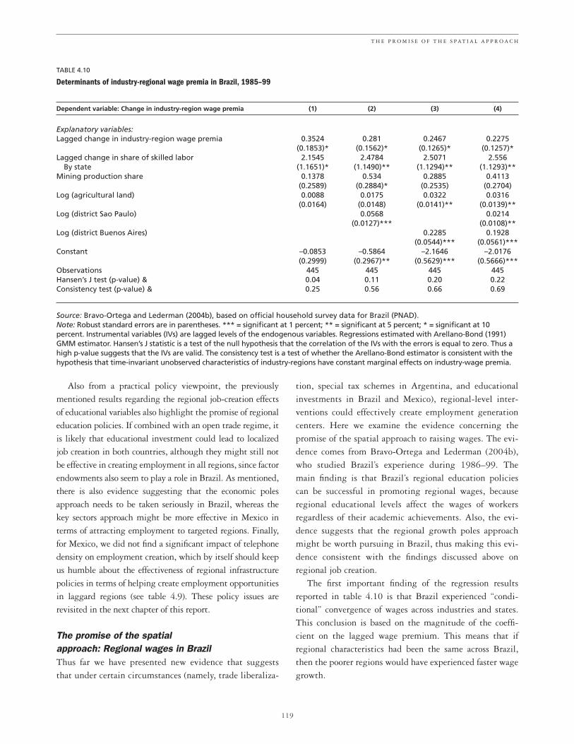
Also from a practical policy viewpoint, the previouslymentioned results regarding the regional job-creation effectsof educational variables also highlight the promise of regionaleducation policies. If combined with an open trade regime, itis likely that educational investment could lead to localizedjob creation in both countries, although they might still notbe effective in creating employment in all regions, since factorendowments also seem to play a role in Brazil. As mentioned,there is also evidence suggesting that the economic polesapproach needs to be taken seriously in Brazil, whereas thekey sectors approach might be more effective in Mexico interms of attracting employment to targeted regions. Finally,for Mexico, we did not find a significant impact of telephonedensity on employment creation, which by itself should keepus humble about the effectiveness of regional infrastructurepolicies in terms of helping create employment opportunitiesin laggard regions (see table 4.9). These policy issues arerevisited in the next chapter of this report.

The promise of the spatial approach: Regional wages in BrazilThus far we have presented new evidence that suggeststhat under certain circumstances (namely, trade liberaliza-

tion, special tax schemes in Argentina, and educationalinvestments in Brazil and Mexico), regional-level inter-ventions could effectively create employment generationcenters. Here we examine the evidence concerning thepromise of the spatial approach to raising wages. The evi-dence comes from Bravo-Ortega and Lederman (2004b),who studied Brazil’s experience during 1986–99. Themain finding is that Brazil’s regional education policiescan be successful in promoting regional wages, becauseregional educational levels affect the wages of workersregardless of their academic achievements. Also, the evi-dence suggests that the regional growth poles approachmight be worth pursuing in Brazil, thus making this evi-dence consistent with the findings discussed above onregional job creation.

The first important finding of the regression resultsreported in table 4.10 is that Brazil experienced “condi-tional” convergence of wages across industries and states.This conclusion is based on the magnitude of the coeffi-cient on the lagged wage premium. This means that ifregional characteristics had been the same across Brazil,then the poorer regions would have experienced faster wagegrowth.

119


TABLE 4.10

Determinants of industry-regional wage premia in Brazil, 1985–99

Dependent variable: Change in industry-region wage premia (1) (2) (3) (4)

Explanatory variables:Lagged change in industry-region wage premia 0.3524 0.281 0.2467 0.2275

(0.1853)* (0.1562)* (0.1265)* (0.1257)*Lagged change in share of skilled labor 2.1545 2.4784 2.5071 2.556

By state (1.1651)* (1.1490)** (1.1294)** (1.1293)**Mining production share 0.1378 0.534 0.2885 0.4113

(0.2589) (0.2884)* (0.2535) (0.2704)Log (agricultural land) 0.0088 0.0175 0.0322 0.0316

(0.0164) (0.0148) (0.0141)** (0.0139)**Log (district Sao Paulo) 0.0568 0.0214

(0.0127)*** (0.0108)**Log (district Buenos Aires) 0.2285 0.1928

(0.0544)*** (0.0561)***Constant –0.0853 –0.5864 –2.1646 –2.0176

(0.2999) (0.2967)** (0.5629)*** (0.5666)***Observations 445 445 445 445Hansen’s J test (p-value) & 0.04 0.11 0.20 0.22Consistency test (p-value) & 0.25 0.56 0.66 0.69

Source: Bravo-Ortega and Lederman (2004b), based on official household survey data for Brazil (PNAD).Note: Robust standard errors are in parentheses. *** = significant at 1 percent; ** = significant at 5 percent; * = significant at 10percent. Instrumental variables (IVs) are lagged levels of the endogenous variables. Regressions estimated with Arellano-Bond (1991)GMM estimator. Hansen’s J statistic is a test of the null hypothesis that the correlation of the IVs with the errors is equal to zero. Thus ahigh p-value suggests that the IVs are valid. The consistency test is a test of whether the Arellano-Bond estimator is consistent with thehypothesis that time-invariant unobserved characteristics of industry-regions have constant marginal effects on industry-wage premia.

Regional-level education also seems to be an importantpredictor of wage premia. In this instance, it is noteworthythat these effects are strictly spillovers, since the estimationof the regional wage premia controls for the individualcharacteristics of workers. In other words, a worker of agiven level of experience and education earns higher wagesif he or she works in regions where the workforce has highaverage education levels. These results can be explained bypositive externalities coming from more qualified workersto the rest of the local labor force.

Regarding the role of factor endowments, we found thatregions with a higher share of mining production haveincreased their wage premia more than others. The evi-dence also suggests that agricultural land has a positiveimpact on wages. There is inconclusive evidence on theimpact of industry concentration. Finally, an importantfinding is the declining strength of the wage gradient withrespect to the economic poles of MERCOSUR, for eitherSao Paulo or Buenos Aires. In turn, this decrease in a spatialwage premium gradient implies a geographical conver-gence of wage premia in Brazil as a whole.

The main policy implication of these findings is that thetrade reforms in Brazil were associated with “conditional”convergence of wages across regions and industries. The factthat the expected geographic wage gradients became lessstrong also suggests that trade liberalization allowed regionsfarther away from the expected economic centers to providebetter-paying jobs. In simple words, trade reforms stimulatewage improvements in geographically disadvantaged regions.Consequently, as trade reforms continue, infrastructure poli-cies aimed at promoting high-paying jobs do not need to linkgeographic areas to the major demand centers as much as inthe context of a closed economy. Rather, it is worth looking atinfrastructure policies that link potentially viable economicregions to closer or local economic poles, as we already men-tioned above. This is in fact the strategy that University ofCalifornia at Berkeley’s Alain de Janvry and others support.

Also from the viewpoint of other territorial develop-ment policies, the empirical evidence suggests that educa-tional policies have a good chance to promote theemergence of high-paying job clusters. And discriminatingagainst mining and agricultural activities might be self-defeating, as they do seem associated with increasing wagepremia. Finally, we found little evidence of persistence ofwage premia over time (that is, we found strong conver-gence in wage premia), which bodes well for the territori-ally focused policies in Brazil’s development.

The spatial approach is promising: Patterns of frontier settlement in Brazil11

Some of the literature reviewed above, especially the eco-nomics of agglomeration, tells us that urban development islikely to be a critical factor in determining the benefits ofopening new frontiers or developing certain regions withincountries. It suggests that to empirically address the benefitsof opening new frontiers in Latin America and theCaribbean, we need to take into account the relationshipbetween pioneers’ choice of economic activities and theaggregate effect of this choice on urban development. In par-ticular, individual household decisions that in the aggregateresult in low population densities and/or low multipliereffects may, in the long run, inhibit the region’s growthpotential. Areas where urban growth is depressed do notdevelop the innovation, learning, and links to global marketsassociated with urban agglomeration effects, nor do theytend to provide the options of nonfarm rural employmentassociated with higher density and urban development.

The evidence discussed in the following paragraphs sug-gests that key economic activities are associated with sus-tainable improvements in economic welfare, and theexpansion of crop agriculture is associated with closer link-ages with urban centers, higher average incomes of the rel-evant population, and less deforestation than livestockactivities that require expansion of land to be used for pas-ture. On the one hand, these outcomes could be endoge-nous to preexisting regional characteristics (weather, soils,and preexisting infrastructure networks), but we believethat some of the observed patterns are due to exogenousvariations that make these findings relevant for policy for-mulation: RDPs that aim to stimulate sustainable use offrontier forest lands should consider the potentially fruitfulroles that can be played by key sectors (crop agriculture)and infrastructure investments that reduce the costs of geo-graphic distance between the frontier areas and nearbyurban growth poles.

The following sections examine patterns of frontier set-tlement and exploitation in the Brazilian Amazon regions.This case study is relevant for understanding the long-termconsequences of policies that might lead to the settlementof low-population-density areas more generally. In addi-tion, these experiences link the economic analysis ofemployment creation and wages with the complexities ofenvironmental degradation, especially deforestation, whichwas previously analyzed in chapter 3 of this report, butmainly from the sectoral viewpoint.

120


Influenced by the literature on rural nonfarm employmentand the territorial approach to rural development (such asAndersen et al. 2002), Chomitz, Schneider, and Thomas(2004) investigated the interaction among rural activities,urban development, and the sustainability of regionalincomes. Of particular relevance for policy discussions, theauthors used a statistical technique (three-stage least squares[3SLS]) that allowed them to not only examine the effect ofland use and population on income, but also to look at possi-ble “feedback” effects of urbanization on land use and averageincomes in the Brazilian Amazon frontier during the past 20years. The existence of feedback effects produces path-dependent development, whereby initial conditions, such assoil quality and climate, lead to the selection of farming activ-ities. In particular, these natural conditions provide the con-text in which settlers chose either to produce crops or cattle.Subsequently, the links with urban centers and/or the pace ofurbanization produces income effects due to the emergence ofeconomies of scale in transport and other factors that are crit-ical for the productivity of agricultural and other rural eco-nomic activities. Figure 4.1 illustrates the main findings fromthe Chomitz, Schneider, and Thomas study.

The arrows depict the causal effects and the numbers pro-vide the magnitudes of the estimated effects. For example, anincrease of 1 percentage point in the share of cleared landthat is used for pasture (cattle ranching) was associated with

an increase of about 30 reais per household for each unit ofland cleared. The effect of an analogous increase in the shareof land cleared for crop production leads to an improvementin average incomes of 95 reais. Moreover, pastureland wasassociated with less urbanization: An increase of 1 percentagepoint in pastureland “caused” a decline of 1 percent in theratio of urban population per unit of cleared land. In con-trast, increases in cropland produced urbanization increases.In turn, urbanization itself increases incomes and increasescropland coverage. Thus frontier settlements that, due tonatural conditions, resulted in the production of crops areassociated with a virtuous cycle whereby cropland increasesincomes and urbanization, which then leads to more crop-land and so on. Pastureland, on the other hand, while it doesmodestly increase household incomes in frontier lands, tendsto reduce the extent of urbanization, leading to less land ded-icated to both crops and lands, thus resulting in subsequentnegative effects on income.

This Brazilian frontier settlement case study clearly illus-trates how certain regions in countries can fall into a “bad”equilibrium, depending on certain natural conditions com-bined with human actions undertaken in the course of his-tory. Such cases can be found throughout the world and LatinAmerica and the Caribbean is not an exception, and the phe-nomenon of the emergence of illicit crops in various countriesand regions within countries is another example (see box 4.1).

121


FIGURE 4.1

Path dependency in Brazilian frontier settlements: Econometric evidence

Income change(monthly totalhouseholdincome-cleared land,in reais)

Annual crop change(annual crops-cleared land)

Planted pasture change(planted pasture-cleared land)

Urban population change(urban population-cleared land)

–0.3

–1.0

0.2

2.3

154

95.0 30.1

Source: Chomitz, Schneider, and Thomas 2004.

While the unsustainable degradation of natural habitats canbe quite costly (see chapter 3), the economic outcomes can bequite discouraging. From a policy viewpoint, we must con-sider approaches that safeguard the environment and offeralternative economic opportunities for poor families whosedespair does not offer them the opportunity to internalize thelong-run negative effects that their private actions can haveon other community members and future generations.

4.5 Summary of analytical findingsThis chapter posed a key policy question concerning thepromise of public policies that aim to bring good jobs to par-ticular regions within countries. Overall, the evidence ispromising, because policy-sensitive characteristics do seemto affect both the quality and quantity of jobs available interritories in the confines of national borders. And these

effects are regional effects in the sense that they come strictlyfrom the regional traits rather than from the characteristicsof people themselves. In other words, people’s well-being canbe affected by the regional characteristics above and beyondthe consequences of individual characteristics. For example,for an individual worker’s given education level, his or herwage will also depend on the educational characteristics ofthe community that surrounds him or her.

Yet these findings are a double-edged sword. That is,regional characteristics, such as soil types, climates, andeven lack of law and order, can lead to poor developmentaloutcomes. The latter can have various symptoms, rangingfrom low incomes combined with environmental degrada-tion (as in certain regions in Brazil’s Amazon frontier) tothe emergence of illicit crop cultivation in regions andcountries where law and order is poor to begin with.

122


The cultivation of illicit crops (namely coca and opium)remains a mystery to many. In fact, it remains a puzzle asto why more countries are not involved in the productionof coca and opium, if the potential returns are so attrac-tive (Thoumi 2003). The answer is not simple but maybe attributed, in part, to plant varieties that thrive underspecific conditions. It is also noteworthy that weak lawand order and internal conflict characterize the majorproducers. Economic conditions might also be a relevantfactor, for they determine the set of alternative economicopportunities for farmers.

Regarding natural conditions that can affect whereillicit crops emerge, it is worth keeping in mind thatthe coca plant is commonly found throughout LatinAmerica. But varieties containing the cocaine alkaloid(the basis for cocaine, HCl) are cultivated and convertedprimarily in Bolivia, Colombia, and Peru. It has beenestimated that there are over 200 Erythroxylum (coca)species growing in the Western Hemisphere, but only17 species can be used to produce cocaine. Fifteen of the17 species contain relatively low levels of cocaine alka-loid, and thus are not cultivated. In South America, twospecies and two varieties in each of these species are cul-tivated and prosper under various climates. At the sametime, the methods used to cultivate and harvest coca

leaf differ depending on climate, local tradition, andother factors. The table above describes the various con-ditions in the Andean countries under which coca iscultivated.

The most widely grown coca variety is cultivated onthe eastern slope of the Andes from Bolivia in the southto as far north as central Ecuador. This area of the Andeshas a tropical climate and experiences high amounts of

BOX 4.1

The territorial approach to illicit crop eradication

Major coca regions in Andean territories

Elevation Climate Rainfall Country (m) (F) (ft) Region

Peru 600–1,911 55 12.44 Huallaga Valley

730–1,300 53 1.32–5.94 Cuzco500–1,350 55 6.6–7.26 Ayacucho

Bolivia 1,465–1,830 45 4.00 Yungas200–550 57 13.00 Chapare

Colombia 1,000–2,050 49.5–52 5.00 Southern region: Putamayo, Caqueta, Guaviare, Vaupes

Source: Schaffer Library of Drug Policy, www.druglibrary.org.

In any case, the finding that regional characteristics mat-ter for determining the development paths of regions withincountries immediately calls attention to a long-standingdebate in Latin America and the Caribbean over the appro-priate design of territorial development programs. Thisdebate is the subject of chapters 8 and 9 in this report.

Notes1. This section draws heavily from Hewings (2003).2. We thank Robert Schneider and Ken Chomitz for highlight-

ing the similarities between the rural-urban linkages literature andthe other concepts mentioned above.

123


rainfall. Coca in this region is usually grown between1,650 and 4,950 feet in elevation. Other varieties thrivein the drier regions of Colombia and, to a lesser extent, inRepública Boxlivariana de Venezuela. It is also grown atlower elevations where the climate is generally hotter.Coca is also found in western Brazil in the Amazon basin,southern Colombia, and northeastern Peru, but is pri-marily cultivated by indigenous populations for theirown consumption and is not as high in cocaine alkaloidsas that found in other areas. Thus it is unlikely that nat-ural conditions alone explain the location of illicit crops.

As mentioned in chapter 3 of this report, govern-ments around the world pursue policies that aim to erad-icate or reduce the cultivation of illicit crops. Thesepolicies usually entail a mix of policies that are difficultto coordinate effectively. These include the spraying ofpesticides over areas where illicit crops are located, thefight against the drug cartels that purchase and profitfrom these crops, and the implementation of alternativedevelopment projects.

In a very preliminary research paper, Lederman andWaite (2004) studied the empirical determinants ofthe probability of a country being an illicit crop pro-ducer. Consistent with the ongoing discussion, theseresearchers examined how the probability of being anillicit crop producer is related to natural, economic,and institutional factors. Their results from Probit

econometric models suggest that economic activity andits composition predominate over natural conditions(that is, climate and elevation). Moreover, the RNRsector size is positively related to the probability ofbeing a producer, whereas the non-RNR sector sizereduces this probability. Thus it seems that the factorsthat determine a country’s RNR sector size also pro-mote the emergence of illicit crops. This is an intuitiveresult, since illicit crops likely use the same types ofproduction inputs and use land as the main factor ofproduction. Yet more developed countries, both interms of GDP per capita and, alternatively, in terms ofthe quality of domestic institutions such as law andorder, have a lower probability of producing illicitcrops. While these are preliminary findings, they do atleast suggest that regional characteristics that gobeyond climatic and natural conditions determine thelocation of illicit and legal economic activities. Inother words, legal economic opportunities (especiallyin non-RNR activities) reduce the likelihood that aregion’s workers will choose to participate in alterna-tive illicit activities, while, in turn, law and ordertends to promote the emergence of legal economicopportunities. This interpretation of the statistical pat-terns in worldwide illicit crop production is thus con-sistent with Thoumi’s (2004) theory of competitiveadvantage in illicit activities.

BOX 4.1 continued

3. See http://www.livelihoods.org/. 4. See http://europa.eu.int/comm/archives/leader2/rural-en/biblio/

com-soc/pre.htm. 5. These projects typically provide money directly to local commu-

nities and let them decide what kinds of projects best meet local needs.6. The errors are corrected to take into account the clustering

effects generated by merging micro data with aggregate regres-sors. In our applications, a cluster is defined as a year-countrycombination.

7. This section draws heavily from Larson, León, and Mugai(2004).

8. This section borrows heavily from Sanguinetti and Volpe(2004).

9. The interpretation of this coefficient is as follows. Distancefrom Buenos Aires has a negative effect on employment agglomera-tion: the farther you are, the fewer jobs. The negative interaction tellsus that as tariffs rise, the impact of distance becomes even more neg-ative. When tariffs decline, the effect of distance becomes less impor-tant as the impact of distance becomes less negative.

10. This section borrows heavily from Bravo-Ortega and Leder-man (2004b).

11. This subsection borrows heavily from research done byChomitz, Schneider, and Thomas.

124


PART II

The Rural Contribution to Development: Policy Issues

127

CHAPTER 5

Public Expenditures, RNRProductivity, and Development

THIS AND SUBSEQUENT CHAPTERS ADDRESS SPECIFIC POLICY AREAS THAT SHAPE RURAL

development’s contribution to national welfare in Latin American and Caribbean countries.This part of the report thus covers policy issues related to the performance of RNR activitiesand issues related to the development of rural territories within countries. In other words, wecover policies that can be viewed through the lenses of either the sectoral or spatial approaches

discussed in chapters 1–4. This chapter in particular covers topics related to the role of public expendituresin shaping the performance of RNR activities and national welfare. The focus gradually shifts to territorialdevelopment policies as the reader moves from chapter 6 to chapter 9.

More specifically, this chapter begins with an analytical evaluation of how public expenditures can beallocated across the rural and urban sectors to maximize the social benefits of scarce public resources. Themain conclusion is that this allocation decision depends critically on two factors, namely the effectiveness(or efficiency) of public expenditures in lifting RNR or agricultural incomes and on the effect that RNRactivities have on the rest of the economy. The latter was estimated in chapter 3, where we found that LatinAmerican and Caribbean RNR activities make substantial contributions to national development to thetune of approximately twice the sector’s GDP share. Thus the rest of this chapter turns to issues related tothe impact of public expenditures on agricultural incomes and poverty.

the production of RNR products. We find that infrastruc-ture, especially roads during the 1990s, were crucial forRNR productivity growth in Latin American andCaribbean countries. Nevertheless, we also find that theremight be important differences across Latin American andCaribbean countries that require further analysis. Thisinternational evidence is complemented with detailedcountry case studies for Ecuador, Mexico, and Nicaragua.The evidence as a whole is quite strong in suggesting thatthe expansion of the agricultural frontier or the expansionof the size of land plots dedicated to RNR production doesnot necessarily raise productivity, which actually dependscrucially on the availability of public goods and comple-mentary factors of production.

Sections 5.2–5.4 study how the structure of public ruralexpenditures in Latin American and Caribbean countriesaffects agriculture and rural poverty. The main messagesfrom our preliminary statistical analyses are that first, LatinAmerican and Caribbean rural expenditures are severelyhampered by excessive private subsidies offered to producers,thus reducing public investments in the provision of publicgoods that have salutary effects on the RNR sector. Second,there is a substantial underinvestment in rural areas and ruraleconomic activities, which might be hampering primarilythe emergence and growth of nonfarm economic activities.

Section 5.5 concludes this chapter by exploring how theprovision of public goods, such as infrastructure, deter-mines the productivity of land, labor, and capital used in

5.1 National welfare and the allocation of public expenditures1

One of the key roles of central governments is to guidethe allocation of public resources in the national economy.Policy makers usually face two broad types of motivationsaffecting allocation decisions. On the one hand, politi-cians have constituencies and interest groups, and voterspermanently pressure them by seeking special favors fromthe public sector. On the other hand, policy makers areconcerned about national welfare. This section provides aframework that identifies the key parameters that welfare-oriented policy makers need to know to assess whether thestructure of public expenditures is optimal from a nationalwelfare viewpoint. The focus is on the distribution ofexpenditures between “urban” and “rural” sectors of eco-nomic activity. The policy maker’s challenge is thus todecide how to distribute the government’s budget, G, intorural and urban expenditures, GR and GU, so that G =GR+GU. A simplifying assumption is that G is given priorto the allocation decision. So the policy decision affectsonly the distribution of G and is not related to the overallgovernment size.

The welfare-oriented policy maker is concerned withmaximizing national welfare, W, which is affected by theperformance of the rural and urban sectors. In turn, publicexpenditures, GR and GU, are believed to positively affectthe growth or size of these two sectors, although inefficientexpenditures focused on providing private subsidies asopposed to public goods could hamper economic growth(see López 2004 and section 5.2). Thus, there are two rele-vant parameters: the sensitivity of national welfare withrespect to sector performance and the sensitivity of sectoralperformance with respect to sector public expenditures.The former was discussed in chapter 3, and thus the follow-ing subsection proposes a simple welfare-based rule fordetermining the marginal public expenditure’s optimaldistribution.

Welfare and optimal allocation of public expendituresSuppose we have a utility function that has as argumentsthe size of the rural and urban sectors. Suppose, in turn,that the rural economy’s output is a function of publicexpenditures in the rural economy. This welfare functioncan be written as follows:

(5.1) ,W W R U W R G U GR U= = ( )( , ) ( ), ( )

128


where W stands for national welfare, R represents rural eco-nomic activities, U represents nonrural activities, and theG’s are sector public expenditures.

The policy maker aims to maximize welfare after thetotal public sector budget has been determined. Thus eachexpenditure unit dedicated to the rural sector comes out ofthe urban budget or vice versa. Hence the contribution of amarginal increase in GR to W is the difference between theeffects of GR on W minus the forgone gains in W due to areduction of GU:

(5.2) .

The policy question is how to allocate resources betweenrural and urban expenditures so as to maximize nationalwelfare. In other words, the policy maker needs to find theoptimal ratio between rural and urban expenditures. Byadding the second term in (5.2) to both sides of the equa-tion and then dividing both sides of the resulting equalityby W, followed by some additional algebra, the optimalratio of rural over urban expenditures becomes:

(5.3) ,

where the a’s are elasticities.2 Equation (5.3) says that theratio of rural over urban expenditures has to be equal to theratio of the welfare elasticity with respect to each sectortimes each sector’s elasticity with respect to the corre-sponding sector’s public expenditures.

This is straightforward in theory, but complicated inpractice. The reason is that a policy maker would need tohave empirical measures of the relevant elasticities. Forexample, we need to know how rural development respondsto rural public expenditures and how, in turn, national wel-fare responds to rural development (the numerator of theright hand side of equation [5.3]) and compare these esti-mates with those for the urban sector. This requires anempirical evaluation of the effectiveness of rural and urbanexpenditures and an understanding of how rural and urbandevelopment affects national welfare.

Bravo-Ortega and Lederman (2005) and chapter 3 pro-vide regional estimates for aW,R and aW,U, based on interna-tional data, but assuming that R is RNR output and U isnon-RNR output. These authors also propose a nationalwelfare function that goes beyond GDP per capita byassuming that national welfare also depends on the average

G

G

a a

a aR

U

W R R GR

W U U GU

=⋅⋅

, ,

, ,

∂∂

= ∂∂

∂∂

− ∂∂

∂∂

=W

G

W

R

R

G

W

U

U

GR R U

0

income of the poorest households, environmental out-comes, and risk. Moreover, since these authors estimateRNR’s or rural growth’s impact on national GDP percapita, this entails estimating cross-sector effects. That is,the authors estimate rural development’s impact on urbandevelopment and vice versa. Thus their estimates of thesectoral welfare elasticities include not only the directeffects of the rural and urban sectors on welfare, but alsothe indirect effects via their influence on each other.

Estimating these parameters or the efficacy of rural andurban expenditures remains a subject for future research.The following section discusses the relationship betweenthis general welfare approach to allocating public expendi-tures and a commonplace technique used for assessing thesector biases of public expenditures, namely the so-called“benefit incidence” analysis of such expenditures.

Welfare and benefit-incidence analysesInformed analyses of the sector distribution of publicexpenditures often use the so-called “benefit incidence”approach. This data-intensive approach requires householdsurveys that contain data on transfers and in-kind servicesreceived by rural and urban households. It is common tosee this application in analyses of what portion of publicexpenditures is received by rural and urban populations,usually focusing on poor households (see, for example,Scott 2004 on the Mexican case).

This approach is a special case of the more general welfareapproach. First, the focus on the value of public expendituresreceived by poor households entails a poverty-focusednational welfare function. That is, the analyst implicitlyassumes that national welfare is synonymous with the wel-fare of poor households and that the latter depends exclu-sively on the pecuniary value of income sources, includingthe value of transfers and in-kind goods and services that thegovernment provides. Second, the benefit incidenceapproach implicitly relies on the assumption that each dollaror peso spent in rural and urban areas has the same rate ofreturn in terms of poverty reduction.3 Consequently, the tra-ditional benefit incidence approach portrays a rural bias inpublic expenditures whenever the value of public-sectortransfers and services received per rural poor is larger thanthat received by the average urban poor.

Although the benefit incidence approach is informativeand is superior to no empirical counterpart to the politicaldecision of how to distribute public funds across sectors, itis worthwhile to be explicit about this approach’s limita-

tions. The most important one is related to the second issueraised in the previous paragraph, namely the assumptionthat the rates of return (in terms of reducing poverty) are thesame across sectors. This is important because it is expectedthat delivering social services is generally more expensive perbeneficiary in rural areas, where population density tends tobe lower than in cities. Thus higher unit costs in the deliveryof services might be driving findings of higher public expen-ditures on the rural poor than on the urban poor. This doesnot mean that policy makers should ignore the costs, butrather that the benefit-incidence analysis might be strictlydriven by costs instead of social benefits. The following sec-tion examines another common and related methodologyused for allocating public expenditures.

The sector shares approachConventional wisdom dictates that governments shoulddistribute their expenditures according to each sector’sshare in the national economy. This view is also a specialcase of the general welfare approach. First, it presumes thateach sector’s marginal contribution to national welfare isequal, which would justify using sector shares as bench-marks for the distribution of national expenditures. Sec-ond, this approach implicitly uses the assumption that themarginal contributions of public expenditures to each sec-tor are also equal.

It is noteworthy that the sectoral shares approach isidentical to the benefit incidence approach when poverty isthe target in the national welfare function. If the policymaker is concerned only with reaching the poor, then allo-cating public expenditures so that each poor family,whether rural or urban, receives the same amount of bene-fits is the same as allocating expenditures according to theshare of poor families found in each sector.4

Can we do better?Thus the question is whether welfare-oriented policy mak-ers can do better than the benefit-incidence or the sectorshares approaches. Again, in theory they can do much bet-ter, but this requires knowledge about the effectiveness ofrural and urban expenditures, as well as a broader view ofnational welfare. In turn, this requires rigorous evaluationsof the impact of various public expenditures on each sector’swelfare. In the case of a poverty-focused welfare function,this requires knowing how effective sector-specific publicexpenditures are in reducing poverty, beyond the value ofbenefits that private agents or households receive. That is, it

129

P U B L I C E X P E N D I T U R E S , R N R P R O D U C T I V I T Y, A N D D E V E L O P M E N T

requires knowing the marginal social returns of suchexpenditures. The following section sheds some light onthese issues.

5.2 Are there policy biases in Latin American andCaribbean countries against rural development?Policy biases against rural development come in the form ofa pattern—across regions and economic sectors—of gov-ernment expenditures on infrastructure, social services, andsubsidies, and of trade and price policies. The issue of tradepolicy and its effect on agriculture specifically is treated insome detail elsewhere.5 This section examines two factorsassociated with a policy bias against rural economic activi-ties, with a special focus on RNR activities: the level andmix of public expenditures and the role of urban concentra-tion. First, we address the hypothesis of the underprovisionof public goods in rural areas, examining first the mix thenthe level of public spending.

Why worry about the provision of rural public goods?The underprovision of public goods may have importantconsequences for the productivity of private investments.Expenditures on public goods create assets that are comple-mentary with private capital, and an absence of such expen-ditures would both affect the scarcity of human capital6

and result in the underinvestment in a variety of sociallybeneficial projects: R&D, infrastructure, environmentalprotection, and so on (World Bank 2000). These are impor-tant assets that contribute to the productivity of privateinvestments, and their absence or deficiency would consti-tute an obstacle to economic expansion.

Government expenditures are directed toward a mix ofpublic and private goods. The bias in the mix toward onetype of good or the other not only has efficiency implica-tions, but may have important equity implications as well.Government expenditures in (nonsocial) subsidies andother private goods tend to be directed to the wealthiersegments of society, sometimes to the detriment of thepoor. The levels of taxation that accompany the expense ofprivate goods also have negative equity consequences incountries that rely heavily on indirect taxation.

Furthermore, the undersupply of public goods affectsthe welfare of the poor much more than the welfare of thewealthy. This is particularly important for the rural poorbecause they have few assets beyond their labor and perhapstheir land and their access to natural resources. Conse-

quently, the rural poor’s income is sensitive to their abilityto enhance their human capital and to protect their naturalassets; from society’s perspective, both have characteristicsof semipublic goods and both are influenced by expendi-tures on social goods.

The performance of agriculture and the evolution ofrural poverty are likely to depend on economic interdepen-dencies with the rest of the economy and with the rest ofthe world. Much of the direct interactions occur throughmechanisms associated with trade and marketing interven-tions and with public expenditure levels and compositionin the rural sector. In addition, both agricultural produc-tivity and rural poverty may be affected by the nonruraleconomy’s performance, as discussed in chapter 3 of thisreport and also analyzed in Gardner (2002). A dynamicnonrural economy may have positive spillover effects on therural sector and agriculture through higher farm productprices, the greater availability of credit, and new technolo-gies. In addition, better employment opportunities andhigher economywide wages are likely to also have positiveinfluences on rural poverty through both migration to andremittances from urban sectors.

The manner in which the government spends tax rev-enues in the rural sector—the particular mix of goods—isoften insufficiently emphasized and analyzed in the litera-ture. The classification of public expenditures into public (orsemipublic) goods and private goods arises from the concep-tual view that governments should use the taxpayer’smoney to enhance social welfare by providing goods andservices that are undersupplied as a consequence of missingmarkets or market imperfections. While there are somegray areas in characterizing whether a good is public or pri-vate, in practice more often than not the distinction is quitesharp. Notwithstanding the debate regarding whether ornot governments spend enough in rural areas or on agricul-ture,7 the structure or composition of expenditures in ruralareas (including, of course, in agriculture) in terms of pub-lic versus private goods is often overlooked.

Subsidies and agricultural performanceInvestment in public goods provides factors of productionthat, almost by definition, the private sector rarely sup-plies, although there is often a complementary relationshipbetween public goods and private investments. Govern-ment expenditures in private goods and subsidies, by con-trast, finance assets with returns that private interestscapture. The effect of these subsidies is almost always detri-

130


mental to economic efficiency and growth and, instead ofcontributing to the promotion of private investment,sometimes they tend to crowd them out, simply increasingthe consumption of the wealthy.

The public provision of private goods or subsidies hastwo negative effects. First, it displaces investment in publicgoods. Government subsidies compete with the provisionof public goods, not only in terms of financial resources,but also in terms of other scarce resources. The administra-tion of subsidy programs often absorbs a large share of lim-ited human capital, and scarce institutional capital is oftenpreferentially allocated to such programs. Subsidiesdirectly crowd out financial and nonfinancial resourcesavailable to governments that could otherwise be used tofund the provision of public goods, such as R&D expendi-tures or infrastructure investments.

Second, subsidies reduce the efficiency of private invest-ments. The existence of subsidies alters incentives forinvestments that are privately (and socially) profitable andcan divert private investments toward activities that wouldotherwise not be privately profitable. Several studies in var-ious countries have shown that subsidies, at least in theform in which they are usually allocated, do not generallypromote investment or more R&D. Empirical studies usingdetailed firm-level data have shown that subsidies and cor-porate tax concessions are at best ineffective at promotingprivate investment and technological adoption.8 Further-more, subsidies also hamper the long-run efficiency of pri-vate investment, because the public expenditure biasestoward subsidies are usually long-run in nature. The lowstocks of public goods caused by continuous underinvest-ment lower the productivity of private investments overthe long run, which is translated into slower investmentand slower productivity growth.9

The structure of public expenditures and rural povertyTwo important components of rural public goods are humancapital and investment in the protection of natural resourcesand the environment. Human capital is the main productiveasset for most poor. As a consequence of credit and othermarket failures, however, in general, the poor are not able tofully finance investments in human capital, regardless ofhow high the rate of return on these investments might be(World Bank 2000). They are, therefore, largely dependenton the public sector as a source of financing for these invest-ments.10 Moreover, the rural poor are also highly dependent

on natural resources as a source of subsistence (Barbier2004). The rural poor often disproportionately pay forresource degradation; investments to protect natural resourcesand reduce environmental externalities are a means to allevi-ate rural poverty.

An inadequate stock of rural public goods contributesto slower growth for agriculture and related rural indus-tries. In general, much of the rural industry linked to agri-culture is highly intensive in unskilled labor, which is theprincipal resource of the poor (as shown in the studies forChile and Mexico), and in many developing countries therural sector’s share in the unskilled labor market is suffi-ciently large to influence significantly the real wages forunskilled workers at the national level. A growing ruralsector is a source of employment for unskilled workers andplays a role in raising wages; consequently, it is a source ofpoverty alleviation.

Econometric evidence of the importance of theexpenditure mix in rural areas in Latin AmericaOne method to ascertain the importance of the mix of gov-ernment expenditures on the rural sector is to estimate itsrelationship to countries’ agricultural GDPs per capita oftheir rural populations. Using data from several LatinAmerican countries on total government expenditures inrural areas and the share of those expenditures in privategoods or subsidies, López (2004) estimates this relationshipcontrolling for trade openness and the per capita GDPshare of the non-agricultural sector. The basic data ongovernment expenditures in rural areas are available for10 Latin American and Caribbean countries for1985–2000.11 Public goods expenditures include those ontechnology generation and transfers, soil conservation, san-itary and phytosanitary protection, communications andinformation services, rural infrastructure, and social ser-vices (for example, education and health). For privategoods, expenditures include commodity-specific or focal-ized items, marketing assistance and promotion, subsidizedcredit, and irrigation.

Table 5.1 summarizes the data on rural expenditures interms of yearly average expenditures for three five-yearperiods. On average, across the nine countries for whichdata are available, between 1985 and 2000 more than 54percent of total rural expenditures was on private goods.But the level and composition of government expenditureshas changed significantly over the period. The share ofspending on private goods (subsidies) has declined notably

131


for most countries, and across all countries fell from 60 per-cent for the five-year period 1985–1990 to 44 percent for1995–2000. Only for Paraguay has the share of subsidiesincreased substantially.

Agricultural growth impact The López results distinguish between “long-run effects” ofthe mix of government rural expenditures, derived frompanel-data estimation using the five-year averages, and“short-run effects” that make use of the data for individualyears.12 The most important message emerging from theseestimates is that, while government expenditures also have apositive effect on agriculture per capita income, the structureor composition of such expenditures is very important. Infact, the results show that, while the short-run effects aresmaller, the long-run marginal effect on agricultural GDP percapita of the share of subsidies in total expenditures (holdingtotal expenditures constant) is surprisingly large and negative(and highly statistically significant): a reallocation of 10 per-centage points of total public expenditures from subsidies topublic goods would increase per capita agriculture income byabout 2.3 percent. And this is obtained without increasingtotal expenditures. By contrast, increasing governmentexpenditures (without changing their composition) is much

less effective in raising per capita agriculture incomes: a 10percent expansion of government outlays causes on averageonly a 0.6 percent increase in agriculture income. Theseimpacts are large mainly because they capture both the posi-tive effect of increasing the provision of public goods and thepositive effect of reducing the distortions created by subsi-dies, which negatively affect the quantity and quality of pri-vate investment, as mentioned above.

In 1996–2000, the 50 percent of the countries thatspent the least in rural areas spent about $35 per capita,while the top 50 percent of the countries spent about $74per capita. If a representative country of the lowestspenders in the region (in terms of per capita expendituresin rural areas) were to spend like the representative highestspender in a region, per capita agricultural GDP wouldincrease by 3 percent. With respect to the share of subsidiesin 1996–2000, it ranged from approximately 30 percentaverage for the bottom half to 65 percent for the top half.This means that if the representative (average) country ofthose that subsidize private goods the most were to readjustits expenditure shares to the level of the representativecountry of those that subsidize private goods the least, itsagricultural GDP per capita would increase, ceterisparibus, in the long term by a substantial 12.5 percent.

132


TABLE 5.1

Government spending in rural areas in Latin America, subsidies and total expenditures (millions of U.S. dollars), 1985–2000

1985–89 1990–94 1995–2000

Countries Subsidies Total Subsidies Total Subsidies Total

Costa Rica 7.5 22.5 34.0 116.2 31.7 127.6(33.3%) (29.3%) (24.8%)

Dominican Republic 164.0 221.4 183.8 243.8 162.0 339.8(74.1%) (75.4%) (47.7%)

Ecuador 59.7 99.2 67.8 102.8 123.3 158.1(60.2%) (65.9%) (78.0%)

Honduras 0.7 7.4 2.0 14.1 7.7 74.7(9.0%) (13.9%) (10.3%)

Panama 109.5 129.7 51.5 65.4 75.9 119.8(84.4%) (78.8%) (63.3%)

Paraguay 72.7 96.2 110.3 139.3 111.1 141.7(75.5%) (79.2%) (78.4%)

Peru 37.8 59.5 288.1 442.5 250.4 578.2(63.5%) (65.1%) (43.3%)

Uruguay 7.3 35.1 6.7 39.9 8.4 43.5(20.9%) (16.7%) (19.3%)

Venezuela, R.B. de 485.7 910.5 176.3 425.8 95.2 352.9(53.3%) (41.4%) (27.0%)

Source: López (2004), based on data from the FAO Latin American and Caribbean regional office in Santiago, Chile.

Poverty reduction impact Although econometrically there is no statistically signifi-cant direct effect on poverty from the level and mix of gov-ernment expenditures (due in part to a lack of rural povertydata), there is statistically robust evidence that growth inRNR GDP contributes to alleviating rural poverty. Mar-ginal changes in non-agricultural GDP also reduce ruralpoverty rates, but the size of their effect is more modest.The public expenditure level and structure have importanteffects on agriculture per capita income and so have indi-rect effects on poverty that are significant. Based on theLópez estimates, a 2.3 percent increase in agricultural GDPper capita (due to a 10 percentage point reduction in theshare of private good spending) would, in turn, induce a1.2 percent reduction in rural poverty. Using the1996–2000 averages for the highest and lowest subsidizers,if the expenditure share on subsidies decreased from 65 per-cent (the average for the highest) to 30 percent (the averagefor the lowest), poverty would decrease 4.2 percent. Sup-posing that 30 percent of the rural population is living inpoverty, with this change in expenditure shares, thispoverty rate would decline to 28.7 percent.

This econometric analysis suggests that the structure ofpublic expenditures is an important economic developmentfactor, and the quantitative importance of this factorappears to be greater than the traditional factors that thedevelopment literature focuses on. In particular, expandingtotal public expenditures in rural areas while maintainingthe existing public expenditure composition does little topromote agricultural income and reduce rural poverty. Thekey issue is not so much how much money is spent in thesector, but rather how public monies are being spent.

The Latin American and Caribbean evidence withrespect to the spending mix is supported by other studies,both country-specific and using cross-country analysis. In adetailed study of India, Fan, Hazell, and Thorat (1999) findthat spending on rural roads and agricultural research andextension has large poverty-alleviation effects and, com-pared with other farm-related expenditures, the largestimpact on agricultural productivity growth.

In a cross-country study of the effects and determinantsof government spending patterns in 43 developing coun-tries, Fan and Rao (2003) find that, with respect to agricul-tural GDP, in general, spending on programs andinvestments related to production agriculture and on educa-tion and roads promoted the sector’s output. And moreimportant for the mix of government expenditures related

to agriculture, R&D outlays enhanced the sector’s produc-tivity more than nonresearch spending. With respect to theinfluence of government spending mix on national eco-nomic growth, the cross-country evidence is less clear. Themarginal effects of all types of expenditures were positivelycorrelated with growth in Asia, and in Africa spending onhealth and the farm sector were significant in promotingtotal growth. For Latin America and the Caribbean, how-ever, the Fan and Rao empirical work finds that only healthspending contributed to growth. This could be due to theinefficient structure of Latin American and Caribbean ruralexpenditures, as mentioned above.

5.3 Disparities in the per capita spending level in urban and rural areasThe evidence of extremely high and nondeclining rates ofreturn suggests that there are important Latin Americanand Caribbean investment opportunities in public goodsthat are not being exploited. An immediate question is,why? Many development economists have pointed to thehistory of bias toward urban areas in national plans toaccount for an insufficient level of public investments—and slower growth—in agriculture and rural areas.13 Thissupposed bias is manifested both in terms of the large dif-ferences between government expenditures per person onsocial services in urban and rural areas and in terms of thediscrepancy between outcomes, such as measured by healthand education levels. Certainly, the data available suggest alarge discrepancy in both spending and outcomes: com-pared with national averages, rural areas receive far fewercentral government resources per person for education (seetable 5.2), and their educational attainment levels are typi-cally lower and school dropout rates higher (see table 5.3).

Distortions in public expenditures on social services andinfrastructure between urban and rural areas would haveconsequences for the marginal productivities of humancapital and other factors in those areas. In the case of educa-tion specifically, human capital formation would be influ-enced by both the supply of education services (the numberand quality of schools) and the demand for those services.Schooling demand is driven, in part, by the potentialreturns to human capital in economic activities in ruralareas (and in urban areas for potential migrants), which isinfluenced by other public investments. The terms of tradebetween rural and urban areas are determined in part bysectoral and trade policies that are not directly related toexpenditures on social services.

133


134


TABLE 5.2

Central government expenditures on education both in rural areas and nationally (U.S. dollars per person)

1995 1996 1997 1998 1999 2000 2001

Money spent on education in rural areasBolivia 2.6 6.1 4.3 3.5 4.0 3.5 —Chile 34.4 47.5 43.2 20.5 18.9 60.1 —Colombia 0.3 0.3 0.3 0.4 1.5 — —Dominican Republic 15.5 19.3 22.7 31.9 38.3 48.3 52.9Ecuador 3.2 2.5 2.0 2.7 2.9 2.6 10.0El Salvador 0.0 20.7 26.0 29.8 32.6 36.3 —Panama — — — 0.1 — — 0.8Paraguay 1.5 1.8 1.9 1.7 0.8 0.3 0.7Peru 7.3 3.7 6.6 2.6 5.6 0.1 1.2Uruguay 1.0 1.0 1.2 1.3 1.3 1.3 1.4Venezuela, R.B. de 11.9 8.0 13.6 15.1 17.4 34.6 30.1

Money spent on education nationallyArgentina 265.0 288.0 — 334.0 350.0 304.0Bolivia 52.0 47.0 — 59.0 57.0 56.0Brazil 220.0 — — — 156.0 167.0Chile 136.0 156.0 181.0 184.0 201.0 208.0Colombia 74.0 87.0 — — — —Costa Rica 115.0 131.0 — — 196.0 174.0El Salvador 36.0 41.0 47.0 46.0 47.0 —Guatemala 25.0 25.0 — 25.0 26.0 29.0Mexico — — — 185.0 218.0 —Nicaragua 13.0 13.0 15.0 21.0 — —Peru — 73.0 — 73.0 68.0 —

Sources: FAO Regional Office, Santiago, Chile, and World Bank 2003a.Note: — = Not available.

TABLE 5.3

Percentage of students reaching three levels of mathematics proficiency, and primary school dropout rates, rural and urban areas

Urban Rural

Dropout rate, Dropout rate, Country Level I Level II Level III primary school Level I Level II Level III primary school

Argentina 96 54 11 — 94 43 6 —Bolivia 94 51 14 2 89 36 8 10Brazil 94 55 15 5 84 40 7 4Chile 95 52 12 4 87 38 6 12Colombia 93 43 6 6 92 50 12 21Cuba 99 90 76 — 99 89 72 —Dominican Republic 81 36 4 4 79 38 7 2Honduras 86 39 8 32 78 23 13 57Mexico 94 58 13 10 90 46 10 24Paraguay 88 42 9 16 82 34 8 36Peru 89 33 4 21 78 23 2 21Venezuela, R.B. de 77 27 3 5 68 22 2 5

Source: UNESCO (2001) Informe Técnico del primer estudio internacional comparativo, August 2001.Note: Dropout rates from Panorama Social de América Latina, CEPAL, 2001–2. Primary school is defined as grades 1–8. — Notavailable.

Relative to urban areas, a policy bias against rural areaslowers incomes reduces the demand for education, which isavailable in fewer and lower-quality schools. The end resultis a tendency for lower rural incomes to persist, and for areduced demand for education. But studies suggest that theimpact of lower human capital formation in rural areas goesbeyond the income generation potential of individualhouseholds. Using panel data of 65 developing countriesthroughout the world (including 19 in Latin America),Chai (1995, cited in Timmer 2002) finds that the urbanpolicy bias reflected in relative educational outcomes inrural and urban areas has an important impact on nationaleconomic growth as well.

A crude measure of the possible bias against rural areasin government expenditures is the share of rural expendi-tures in total, relative to agriculture’s share in nationalGDP, the most important rural industry. This index of gov-ernment expenditures in rural areas is the ratio of two pro-portions: the rural sector’s share of total spending (GR/G),and agriculture’s share of national GDP (GDPA/GDPT):

(5.4) .

When the index is equal to one, a government is spend-ing proportionally in rural areas what agriculture is gener-ating as a share of national income. This index is a broadgauge of how close public spending is to meeting the crite-rion that governments should distribute their expendituresaccording to each sector’s share in the national economy. As

IGER

GG

GDPGDP

R

A

T

=

discussed in section 5.1 above, such an objective wouldonly be consistent with optimizing national welfare undervery special circumstances. In fact, the evidence assessed inchapter 3 suggests that Latin America and the Caribbean’saverage welfare elasticity with respect to agriculture isroughly equal to two times its share in national GDP.14 Ifthe sectoral returns to public expenditures are equal forrural and urban expenditures, also an unlikely propositionunless the structure of rural public expenditures isimproved in most Latin American and Caribbean countriesas argued above, then the optimal IGER would be equal to2. Nevertheless, using this index of relative proportions ofspending to sectoral GDP, one can compare the implicitweights that governments place on their rural sectors acrosscountries and through time.

Table 5.4 shows the evolution of these indices of all gov-ernment expenditures in rural areas for 10 Latin Americancountries for which data are available between 1985 and2000. What is notable from these data is the heterogeneityof the spending index across countries. The indices indicatethat for several countries, in the latter half of the 1990s,rural areas received more than the share of agriculture inthe total economy. This is the case of Chile, the DominicanRepublic, Honduras, Panama, and República Bolivarianade Venezuela. (But remember, an index value of one is not areference point for social efficiency.) For the other half ofthe countries, rural areas receive less than the agriculturalGDP share. Aside from an increase in most countries in thespending index in the late 1990s compared with the mid-1980s and early 1990s, there is no general pattern for theregion. In terms of total spending on all types of goods,

135


TABLE 5.4

Index of government expenditures in rural areas: Share of rural outlays in total spending relative to the share of agricultural GDP, 1985–2000

Country 1985 1990 1991 1992 1993 1994 1995 1996 1997 1998 1999 2000

Chile — — — — — — 0.83 1.37 1.58 1.27 1.12 1.26Costa Rica — 0.13 0.17 0.92 0.87 0.78 0.61 0.65 0.68 0.46 0.39 0.52Dominican Republic 1.94 2.56 3.48 5.63 3.42 3.45 2.69 2.25 2.06 2.25 2.31 2.32Ecuador 0.03 0.05 0.04 0.04 0.04 0.01 0.03 0.04 0.03 0.02 0.04 0.02Honduras 0.09 0.05 0.13 0.15 0.25 0.13 0.32 0.39 0.41 0.65 0.79 1.61Panama 1.32 0.44 0.62 0.58 0.67 0.56 0.64 0.65 0.77 1.50 0.99 1.23Paraguay 0.10 0.82 1.20 — 0.89 0.69 0.85 0.76 0.79 0.59 0.45 0.51Peru 0.25 0.88 1.21 0.80 1.81 1.48 1.50 1.26 1.32 1.06 0.87 0.67Uruguay 0.01 0.01 0.01 0.01 0.02 0.02 0.02 0.02 0.02 0.02 0.02 0.02Venezuela, R.B. de 2.65 1.13 1.36 1.61 1.06 0.82 0.92 0.92 1.31 1.00 0.88 1.37

Source: Calculated based on FAO rural government expenditure data; GDPs from World Bank 2003a.Note: — Not available.

there does not appear to be a systemic bias against ruralareas across Latin American and Caribbean countries. Butgiven the evidence presented earlier, there is very likely asystematic bias in the provision of public goods, such aseducation and infrastructure investments.

5.4 Does excessive urban concentration harm RNR activities and the rural economy?Latin American and Caribbean urbanization levels are highin comparison with other regions and similar to those ofNorth America (see table 5.5). The regional average of thepercentage of the population living in urban areas is cur-rently 75 percent, and by the year 2025, average urbaniza-tion is projected to reach 82 percent (reported in Lattes,Rodríguez, and Villa 2002). Recently growth rates in theregion’s urbanization levels have declined (0.8 percentbetween 1975 and 2000), compared with the periodbetween 1925 and 1950, when the urban growth rate (2percent) was twice that of total population growth.

Historically, Latin America has been notably urbanizedrelative to its degree of economic development. This charac-teristic is sometimes attributed to the initial conditions asso-ciated with the Spanish colonization process (for example, inLattes, Rodríguez, and Villa 2002), to the emphasis on pri-mary production for export (and the consequent growth ofport cities) prior to the early twentieth century, and laterwaves of immigrants to urban centers from outside the region(Lattes, Rodríguez, and Villa 2002). The period of importsubstitution policies, which promoted urban industry prior totrade reforms, has also been implicated in the rapid expansionof regional cities after 1925 (Cerrutti and Bertoncello).

Although it has been the case that, worldwide, the num-ber and size of urban areas have increased with populationincreases, certainly the growth of large cities in LatinAmerica has been striking, as can be seen in table 5.6.

In 1950, 16 percent of South America’s urban popula-tion lived in cities of more than 500,000 and nearly 13 per-cent in cities of greater than 1 million, of which there wereonly five. By contrast, in 1990 nearly 38 percent of theurban population lived in cities of more than 500,000, and32.5 percent lived in cities of more than 1 million, ofwhich there were 31. Moreover, while in 1950 SouthAmerica could claim only one city of more than 4 million,in 1990 there were six.15 The number of South Americanurban areas of greater than 20,000 inhabitants grew from194 in 1950 to 931 in 1990, and in Mesoamerica from 77to 279.

Although the region as a whole can be characterized ashighly urbanized if official criteria are used, the degree ofurbanization varies significantly across countries (see table6.8). In South America, Argentina had the largest percent-age of urban residents in the year 2000 (90 percent) andParaguay the smallest (65.3 percent). In Mesoamerica,Cuba ranked highest in degree of urbanization (75.3 per-cent) and Haiti and Guatemala the lowest (36 percent and40 percent). The degree of urban primacy (the percentageof total urban population living in the largest city) alsovaries in the region, from Panama and Guatemala with over70 percent of their urban populations in the largest city, toBrazil and República Bolivariana de Venezuela with about15 percent urban primacy. In general terms, the smallercountries of Mesoamerica have the highest urban primacy

136


TABLE 5.5

Regional urbanization levels (percent), 1925–2025

Region 1925 1950 1975 2000 2025

Africa 8.0 14.7 25.2 37.9 51.8Asia 9.5 17.4 24.7 36.7 50.6Europe 37.9 52.4 67.3 74.8 81.3Latin America 25.0 41.4 61.2 75.3 82.2North America 53.8 63.9 73.8 77.2 83.3Oceania 48.5 61.6 71.8 70.2 73.3World 20.5 29.7 37.9 47.0 58.0

More developed countries 40.1 54.9 70.0 76.0 82.3Less developed countries 9.3 17.8 26.8 39.9 53.3

Source: Lattes, Rodríguez, and Villa 2002.

TABLE 5.6

Urban population percentages living in cities of differing scales,

1950 and 1990

South America Mesoamerica

Size of cities 1950 1990 1950 1990

More than 1 million 12.7 32.5 7.3 22.5500,000 to 1 million 3.2 5.1 2.2 6.4100,000 to 500,000 7.5 12.1 9.1 1220,000 to 100,000 7.4 12.8 7.2 9.9Less than 20,000 69.2 37.4 74.2 49.2Number of cities of more than 20,000 194 931 77 279

Source: Pinto da Cunha 2002.

levels and the larger South American countries the smallestlevels.

In terms of a simple average across countries included intable 5.7, urban primacy levels have not noticeably changed,although some countries saw significant changes in primacybetween 1960 and 2000, as figure 5.1 demonstrates. Of the21 Latin American countries included in the data for figure5.1, 12 experienced declines in primacy levels. Costa Ricaand República Bolivariana de Venezuela had the largestdeclines of over 40 percent in their primacy levels. The mostnotable primacy increases have been in the small countries ofGuatemala, Guyana, and Haiti, and in one relatively largecountry, Colombia. Primacy measures are generally higher inLatin America than in other parts of the world; certainly allhave much higher levels than that of the United States.

Except for Brazil and R.B. de Venezuela (due to a substantialfall in its primacy level), all Latin American countries havehigher primacy levels than Canada.

How does urban concentration affect the contribution of agriculture and rural areas to the national economy?Economic analyses of the evolution of cities and the role ofurban economies in economic growth16 focus primarily onthe relationships among urbanization, urban concentra-tion, and non-agricultural activities. The agricultural sec-tor specifically and rural activities more generally aretypically not addressed, except insofar as the rural sectorplays an initiating role in the urbanization process, espe-cially as a labor source for industrial employment.17

137


TABLE 5.7

Degree of urbanization and urban primacy in Latin America

Population % Urban (1,000s) urban primacy

2000 2000 1960 2000

South AmericaArgentina 37,032 89.92 0.45 0.37Bolivia 8,329 62.47 0.36 0.28Brazil 170,115 81.28 0.15 0.13Chile 15,211 85.67 0.39 0.42Colombia 42,321 73.9 0.16 0.21Ecuador 12,646 65.33 0.29 0.27Paraguay 5,496 55.99 0.47 0.41Peru 25,662 72.77 0.37 0.40Uruguay 3,337 91.25 0.57 0.43Venezuela, R.B. de 24,170 86.93 0.28 0.15

Central AmericaCosta Rica 4,023 47.85 0.67 0.41Cuba 11,201 75.31 — —Dominican Republic 8,495 65.05 0.46 0.47El Salvador 6,276 46.64 0.32 0.35Guatemala 11,385 39.66 0.41 0.72Haiti 8,222 35.7 0.44 0.61Honduras 6,485 52.74 0.30 0.28Jamaica 2,583 56.1 0.68 0.63Mexico 98,881 74.39 0.27 0.25Nicaragua 5,074 56.13 0.33 0.35Panama 2,856 56.23 0.61 0.73

North AmericaCanada 30,770 78.70 0.14 0.20United States 282,224 77.22 0.11 0.08

Latin America average urban primacy 0.40 0.39World average urban primacy 0.35 0.33

Source: U.N. 2001.Note: — Not available.

Urbanization is considered simply a natural consequence ofdevelopment: labor is released to urban areas as a resultboth of shifts in labor-saving technology taking place at thefarm level and of changes in the composition of nationaloutput toward nonfood production.

Agricultural production and other rural activities takeplace in remote areas and while urban-oriented economicstudies recognize that these activities might be affectedby urbanization and urban concentration, at the center ofattention are questions related to explaining the industri-alization in cities, the patterns of industrial locationamong different cities, and the interrelationships betweennational economic growth and urban system develop-ment. Once the national economy’s rural component hasbeen given a passing acknowledgment, the conversationusually turns to the various reasons for the forms thaturbanization might take: the role of agglomerationeconomies in industrial organization, the distribution andsize of urban centers, the relative importance of localiza-tion and urbanization economies for urban firms and theirchoice of location, and the benefits and costs of (perhapstoo much) urban concentration in one or two metropolises

for the efficiency of industrial production, quality of life,and overall national growth.18

There are costs to what urban economists call “exces-sive” urban concentration; congestion effects in a mega citymay provoke politicians to use public resources and inter-ventions to divert resources from more productive activities(investments and social services) toward the sustaining ofthe quality of life in the metropolis.19 Is the agriculturalsector harmed more or less than other economic sectors bythe costs associated with excessive urban concentration? Allsectors bear the social costs associated with supporting anexcessive level of concentration in a metropolis through theinefficient allocation of resources, but the urban economicsliterature tends to stress the costs borne by industries inmedium-size and smaller urban areas due to underinvest-ment in urban infrastructure and social services outside theprimary city.

The agricultural economics literature has tended, on theother hand, to stress the consequences of an overall urbanpolicy bias for an imbalance of public and private invest-ment (for example, Lipton 1993 and Timmer 2002), result-ing in significant differences between urban and rural areas

138


FIGURE 5.1

Urban primacy levels in the Americas, 1960–2000

0.900

0.800

0.700

0.600

0.500

0.400

0.300

0.200

0.100

0.0

1960 2000

Urban primacy

United St

ates

Brazil

Venez

uela, R

.B. d

e

Canad

a

Colom

bia

Mex

ico

Ecuad

or

Honduras

Bolivia

Nicara

gua

El Sa

lvador

Argen

tina

Peru

Costa R

ica

Para

guayChile

Uruguay

Domin

ican R

epublic

Puer

to R

icoHait

i

Jam

aica

Guatem

ala

Panam

a

Guyana

World

aver

age

LAC av

erag

e

Source: Foster (2004), based on U.N. data.

in the marginal product of physical and human capital.Eliminating obstacles to realizing returns on investment inrural areas due to policy biases favoring urban investmentwould allow improved efficiency in resource flows and anincrease in factor productivity overall (Schultz 1978). Tim-mer (2002) specifically addresses the possible policy biasfavoring urban human capital development, manifested inpart by a reduced supply of educational facilities and aver-age years of schooling in rural areas.

But there could be benefits from urban concentration,for rural communities and agriculture. The most obviouspotential source of benefits to agriculture would derivefrom concentrated urban populations, similar to thereduced marketing and search costs that urban suppliersand buyers enjoy. After all, urban concentration is also thegeographic concentration of those who want to eat but tendnot to grow their own food. Increases in shipping volumesto centralized distribution points reduce the final cost ofdelivering food to urban consumers, a benefit that can beshared by farmers and consumers through an increase in thefarm gate price and a decrease in the retail store price.Rural-to-urban transport networks are less dispersed,supermarkets and other retailers are larger, advertisingcosts fall with the increase in size of the local intendedaudience, and intra-urban distribution systems can takeadvantage of scale.20

Nonfarming rural activities are likely tied to agriculturein some way, although their contributions to nationalincome would not be accounted for in agricultural GDP.Processing of agricultural products, transport of raw andprocessed goods to urban centers (for final consumption,further processing, or export), and other rural-based activi-ties that add value along the marketing chain from farm tocity would also benefit from urban concentration as theyshare in reduced costs.

Furthermore, industry agglomeration in cities reducesthe costs of urban-produced goods and services demandedby rural economic activities. The benefits of the localizationeconomies for firms of standardized products in medium-size and small cities would likely not be the result of con-centration per se in the metropolis. But indirectly, byreducing the costs of the intermediate goods and servicesproduced in the metropolis to standardized firms in smallercities, urban concentration’s benefits would be passedthrough to rural businesses and agriculture, as well as toother sectors. More directly, the largest cities are oftenR&D centers, the focal point of sophisticated finance and

insurance markets, and the entry points of foreign tech-nologies, capital goods, seeds, fertilizers, pesticides, andother inputs; and while imported products might be stan-dardized, the importers’ services of finding foreign sourcesand domestic buyers for a variety of goods are less likely tobe, especially in a developing country.

To the degree that the social costs of excessive urbanconcentration in a metropolis arise from poorer investmentin infrastructure farther from the metropolitan center thanelsewhere, one might initially guess that agriculturewould suffer relatively more from policies leading toexcessive concentration than would industries located inmedium-size and smaller cities. But other considerationswould argue that agricultural GDP, relative to rural non-farm and small city output, might be less negativelyaffected by excessive growth in the metropolis: (1) onewould observe a slower decline in agricultural GDP sharebecause the sector would become relatively less dependenton purchase inputs; (2) agricultural productivity increasesare perhaps more dependent on technological innovationsarising in (or passing through) the metropolis than areproductivity increases in other rural and small city non-farm sectors; and (3) the provision of cheap agriculturalgoods to the primary city would likely be a concern to thesame politicians that favor skewing infrastructure invest-ment to sustain the quality of life of an excessively concen-trated urban population.

Econometric evidence: Urban primacy appears to harm off-farm more than agricultural activitiesA cross-country econometric study21 prepared for thisreport addresses the roles that urban concentration andrural density play in influencing national economic growth,agriculture’s share of total GDP, and agricultural land pro-ductivity. The analysis makes use of data for 83 countriesbetween 1960 and 2000 (in the form of five-year averages)on growth rates, urban primacy, rural population densityper kilometer of arable land, and other determinants ofnational and agriculture sector GDPs. Both urban concen-tration and rural density should positively influencegrowth through local information spillovers, which in turnaffect local knowledge accumulation and agglomerationeconomies. Excessive urban concentration, however, woulddraw resources from productive investment and innovationtoward nongrowth-promoting investments and innova-tions associated with attempts to maintain quality of lifeand economic rents in congested urban centers.

139


The results confirm previous work (Henderson 2002)showing that urban concentration has a nonlinear effect onnational growth rates—positive at low levels of concentra-tion and negative at high levels—and that the effects of con-centration are influenced by country scale. The results alsoshow that observed urban primacy rates are generally exces-sive in terms of economic growth rates. Moreover, the resultssupport the hypothesis that the positive effects of agglomer-ation economies in rural areas on national economic growthare enhanced with greater rural density.22 With respect toagriculture’s contribution to national income, an increase inrural density has a statistically significant negative effect onthe change in agriculture’s GDP share relative to total GDP,becoming less negative with increases in urban primacy andmore negative with increases in schooling. Increases in urbanprimacy, on the other hand, have statistically significant pos-itive impacts on agriculture’s GDP share.

Evidently, the economies induced by greater rural densitycontribute to overall growth by stimulating non-agriculturalactivities more than agriculture. Such nonfarm activities arelikely to be both in rural areas and in medium-size and smallcities that are physically closer to rural areas. But, moreimportant, the results show that while the diseconomiesinduced by excessive urban concentration slow overallgrowth over the range of primacy levels exhibited by mostcountries (using 2000 reference data), including those ofLatin America, they must be doing so by harming non-agri-cultural sectors more than agriculture. The magnitude ofthis effect rises with rural population density; probablybecause less dense rural areas are associated both with fewernon-agricultural rural activities and perhaps because withless rural density there is less economic activity in generalthat takes place in remote urban areas as well. With respectto changes in agricultural land productivity, the analysisshows that the scale economies associated with rural densityand urban concentration positively influence productivity.

Taking together the results for per capita GDP, agricul-ture’s GDP share and land productivity, the agglomerationeconomies associated with urban concentration apparentlydecrease nonfarm sector activities more than farming. They doso both by harming non-agricultural activities and by increas-ing agricultural productivity. The implication is that,although further urban concentration might be excessive froma national growth perspective, the growth in nonfarm ruralactivities would likely be stunted to a greater degree than thegrowth in production agriculture. To the extent that ruralnonfarm activities are becoming a major source of employ-

ment and poverty reduction,23 the consequences of excessiveurban primacy and the diversion of resources to heavily con-centrated urban areas are even more costly to society.

5.5 Sources of RNR productivity growth in Latin American and Caribbean countriesHow fast can RNR productivity grow in Latin Americanand Caribbean countries? Answering this question requiresknowing, first, how fast the productivity of RNR activitieshas grown in Latin American and Caribbean countries com-pared with that observed in some of the most dynamic RNReconomies in the world. Second, we need to identify themain factors that have driven RNR sector productivity invarious Latin American and Caribbean economies. Thesetwo issues are addressed in the following subsections.

RNR productivity growth has been rapid in severalLatin American and Caribbean countriesUnderstanding the drivers of RNR productivity is challeng-ing for a variety of reasons. An important one is that RNRsector products are quite diverse, ranging from fisheries to allsorts of agricultural products. Furthermore, it is quite likelythat the same product can be produced with a variety of tech-nologies, allowing radically different economies to produceproducts that are indistinguishable from each other from theviewpoint of consumers. In other words, maize varieties canbe produced in both the United States and Mexico, but farm-ers in each country probably use dramatically differentmachinery and crop management techniques.

For these and other reasons, the resurgent academic lit-erature on RNR production functions has been recentlydominated by so-called “multi-output” production func-tions applied to international data and to farm-level data.This approach focuses on the factors that explain the valueof RNR production, rather than providing product-specificcomparisons. The underlying reason for this approach isthat both the output mix and the choice of technologiesand management strategies can be simultaneously deter-mined by the quantity of labor, tractors, animals, and soforth, that are used in the production process.

This is the logic of the so-called “translog” production-function approach described in box 5.1. This is a flexibleempirical approach for measuring the rate at which thevalue of any mix of RNR goods is produced for a given levelof use of tractors, workers, animals, land, and so forth,which allows the possibility that the productivity of specificfactors of production can also rise and the utilization of one

140


factor can affect the productivity of another. In other words,we are interested in measuring how the value of productionof RNR products changed over time for a given level of useof the relevant factors of production. In research thatBravo-Ortega and Lederman (2004a) undertook, this

approach was implemented with data from the FAO andthe World Bank. Table 5.8 presents the resulting RNRproductivity growth estimates.

In Latin America and the Caribbean, Brazil is the coun-try with the highest TFPy growth, which averaged 1.93

141


Following Kawagoe, Hayami, and Ruttan (1985) andLau and Yotoupoulos (1989) our initial assumption isthat developed and developing countries exhibit differentproduction functions. In particular, Lau and Yotoupoulos(1989) show that estimating a meta-production functionbased on international data requires paying close atten-tion to differences in the quality of the inputs. To con-sider international heterogeneity in the quality of inputs,first assume that input j of a developed country in termsof the input in a developing country r can be expressed as

, where a Ajr is a conversion factor. Thenthe translog function is expressed as follows:

(1)

,

which is equivalent to:

(2)

;

the previous expression can be simplified to:

(3)

,

where

, and .

Note that in a country in the reference group, all Air

are 1, therefore equation (3) reduces to the regular

translog. To capture the factor-augmentation parametersfor all countries not included in the reference group, theeconometric model needs to include a variable defined asthe interaction between a group-identifying dummyvariable and the corresponding variable for each factor ofproduction.

This report provides estimates of two regression mod-els, one using as a reference group the developing coun-tries and another using the developed countries. In thismanner we avoid the dubious interpretation of the coeffi-cients expressed without tilde, which indeed would allowus to recover elasticities and returns to scale with respectto a reference group. By changing the reference group wecan recover true elasticities for each group and truereturns to scale.

In addition, we are interested in capturing the evolu-tion of technical progress, ideally in a differentiated man-ner for each country. Following Kim (1992) we add atime trend and its quadratic term to model (3), so that wecan capture the average rate of total-factor productivity(TFPy) growth, which is the portion of output growththat is not explained by the utilized stock of factors ofproduction. Finally, we add the interaction of the timetrend variable and the natural logarithm of each factor.This allows us to recover different rates of technicalprogress associated with changes in the returns to eachfactor of production. Therefore our empirical productionfunction is specified as follows:

(4)

.

Source: Bravo-Ortega and Lederman 2004a.

++ ⋅ ( ) + +∑γ δ δiTi

i T TTT X T Tln1

22

ln lnB X Xi

iji

i j+ ⋅ ( ) ⋅ ( )∑ ∑1

2++

ln( ) lnY a a Xii i= + ( )∑0

α α β βi i kr ijk

jiA= + +∑' ln( )( )ln( )jrA

α α α β0 0= + + ⋅∑ ∑∑' ln( ) ( )ii ir ijj

iri

A ln A

ln( ) ln( )X Xijj

i ji

+ ⋅ ⋅∑∑ β1

2

ln( ) ln( )Y Xii i= + ∑α α0

ln( ) ln( )A Xjr j⋅ +( )

ijj

+ ⋅∑β1

2lln( ) ln( )A Xir i

i

+( )∑

ln( )' Xii i+ ∑ α

ln( ) ln( )' 'Y Aii ir= + +∑α α0

ln( )A Xijj

ir i+ ⋅ ⋅∑β1

2lln( )A Xjr j

i∑

ln( ) ln( )' 'Y A Xii ir i= + ∑α α0

X A Xj jr j* = ⋅

BOX 5.1

Empirical translog production functions

percent per year during 1960–2000. Mexico follows Brazilwith an average increase of 1.85 percent. In the third posi-tion and very close to Mexico’s average is Argentina, with a1.84 percent increase. On the last spot of our sample is ElSalvador, with an average increase of 0.53 percent. Thenext-to-last spot is occupied by Paraguay, with an averageincrease of 0.74 percent per year.

Regarding the high-income countries, the highest TFPygrowth was in Australia with 2.17 percent per year, fol-lowed by the United States with an average TFPy increaseof 2.04 percent. France occupies the third spot with a TFPyincrease of 1.74 percent per year. Finland holds the last spotwith a very low 0.21 percent. Among the non-Latin Amer-ican and Caribbean developing countries, India led the

group with an average TFPy increase of 1.98 percent, fol-lowed by China (1.67 percent) and Indonesia (1.45 per-cent). Among the lowest TFPy growth in the full sample isMozambique, with a reduction of 0.04 percent per year.

Average TFPy growth for high-income countries is 1.36percent per year, followed by Latin America and theCaribbean with an average increase of 1.2 percent. The restof the poor countries show an average of 0.74 percent. It isclear that several Latin American and Caribbean countries,including Argentina, Brazil, and Mexico, were, in fact, ableto achieve relatively high rates of RNR productivity growthduring the period under study, namely 1960–2000. Theseresults are consistent with recent studies that have alsofound quite rapid agricultural productivity growth in

142


TABLE 5.8

Total factor productivity growth in RNR activities in Latin America and the Caribbean (LAC) and around the globe

TFP growth TFP growth Average TFP over 40 Average TFP over 40growth (%) years (%) growth (%) years (%)

Argentina 1.84 107.61Bolivia 1,18 60.13Brazil 1.93 114.44Chile 1.20 61.32Colombia 1.43 76.65Cuba 1.17 59.10Ecuador 1.28 66.23El Salvador 0.53 23.31Guatemala 0.79 36.83Haiti 0.97 46.95Honduras 0.78 36.38Mexico 1.85 108.54Nicaragua 0.79 36.98Paraguay 0.74 34.34Peru 1.36 71.81Venezuela, R.B. de 1.35 70.97

LAC average 1.20 63.22

Australia 2.12 131.84Austria 0.69 31.79Canada 1.23 62.95Finland 0.25 10.50France 1.77 101.76Germany 1.39 73.37Greece 1.62 89.85Ireland 0.72 33.50Italy 1.73 98.59Japan 1.40 74.31Netherlands 1.16 58.55Portugal 1.41 75.02Spain 1.89 111.50

United Kingdom 1.67 93.64United States 2.11 130.77

High-income average 1.36 75.51

China 1.67 94.10Hungary 1.14 57.15India 1.98 119.17Indonesia 1.45 77.90Iraq 1.13 56.46Kenya 0.78 36.23Malaysia 1.21 61.58Mali 0.63 28.54Mauritania 0.40 17.38Morocco 1.22 62.49Mozambique –0.04 –1.40Myanmar 0.90 43.24Nepal 0.69 31.90Niger 0.37 16.09Philippines 1.44 77.09Romania 1.42 75.42Rwanda –0.01 –0.27Saudi Arabia 0.61 27.79Somalia 0.68 30.93Sri Lanka 0.95 46.07Sudan 0.96 46.40Thailand 1.39 73.58Tunisia 1.21 61.60Turkey 1.56 85.73Uganda 0.62 28.19Vietnam 1.09 54.52

Other countries average 0.74 37.62

Source: Bravo-Ortega and Lederman 2004a.Note: Average and cumulative growth rate of RNR TFP derived from empirical translog production function.

developing countries (Ninn et al. 2003) and with existingevidence on the relatively fast growth of agricultural TFPyin developed countries (Martin and Mitra 2001). The find-ing that high-income countries have experienced high pro-ductivity growth rates cannot be used to support theirprotectionist policies, because these and other agriculturalproductivity estimates come from historical data (from1960–2000 in our case; from 1967–92 in the case of Martinand Mitra), while the protectionism of agricultural activi-ties strengthened substantially in the United States andEurope after the mid-1980s. In fact, it is possible that com-petitive pressure emanating from imported agriculturalproducts might have been an important driver of agricul-tural efficiency in the high-income countries. However,from a policy viewpoint, it is perhaps more important tounderstand the types of factors that are limiting furtherRNR productivity growth, especially in recent times.

RNR productivity in Latin America and Caribbean countries is limited by inadequate public goodsTo study the TFPy determinants across countries, it is easierto estimate what economists call a “Cobb-Douglas produc-tion function” instead of the more flexible translog functiondiscussed above. The main reason is that the analysis needs tocontrol for the contribution of factors of production (tractors,animals, land, and labor) as well as factors that influence thecontext in which RNR production is taking place. For exam-ple, infrastructure coverage or the depth of domestic finan-cial markets might affect not only the stock of the factors ofproduction that are available within each economy, but theymight also influence the efficiency with which these factorsare used. Alternatively, one can think of these country char-acteristics as the determinants of how much capital, labor,land, and human capital are used for the production of RNRgoods and that mix is automatically or endogenously deter-mined by the same factors. For these reasons, the resurgentscientific literature on RNR production efficiency has beendominated by multi-output production functions applied tointernational as well as farm-level data (see Mundlak 2001).

This section follows this alternative Cobb-Douglasapproach. Moreover, due to the slimmed-down Cobb-Douglasproduction approach, Bravo-Ortega and Lederman (2004a)were able to deal with the difficult econometric issue of theendogeneity (or reverse causality) going from RNR produc-tion to the decisions that farmers make to buy additional trac-tors or hire additional workers. At the country level, this

approach is similar to now common approaches used forunderstanding why some countries develop faster economi-cally than others, such as the cross-country regression approachpioneered by Barro (1991). It is similar in that the fundamen-tal sources of economic growth are thought to be determinedby each country’s structural and policy characteristics.

The following paragraphs discuss evidence concerning theRNR productivity growth drivers in Latin American andCaribbean countries and in the rest of the world. It is notewor-thy that the factors analyzed herein are measured at the coun-try level and thus do not reflect the incidence of rural publicgoods per se, but rather the overall national coverage of the rel-evant factors. For example, to study the impact of credit avail-ability or roads, we use the national ratio of credit to theprivate sector over total GDP and the national total of pavedroads per kilometer, rather than agricultural credit or ruralroads. This is consistent with the theory discussed above thattreats a country’s output mix as endogenous to national char-acteristics. Nevertheless, the direction of the empirical effectsof the studied variables could be interpreted as indications ofwhether the national provision of public goods has favoredRNR or agricultural productivity or whether the provision ofpublic goods has suffered from an “urban” bias.

Table 5.9 reports estimated effects on RNR TFPygrowth for the Latin American and Caribbean region as a

143


TABLE 5.9

The effect of public goods on RNR-sector productivity growth in

Latin America and the Caribbean (LAC) and the rest of the world

Effect in LAC Effect in the rest of the in the 1990s world during 1960–1999

Illiteracy –0.024 –0.0190.000 0.000

Irrigation 0.120 0.0340.180 0.560

Roads 0.424 –0.2090.000 0.000

Telephone density 0.063 0.0620.140 0.020

Credit to private sector 0.001 –0.0010.150 0.020

Electricity generation 0.027 0.0760.380 0.000

Source: Bravo-Ortega and Lederman (2005) providedpreliminary econometric estimates. Note: Effect of a 1 percent increase of each variable on theaverage annual growth of RNR total factor productivity; p-values of elasticities are listed under each estimate.

whole during the 1990s. For comparison, this table alsoprovides consistent estimates for the rest of the world dur-ing the 1960–2000 period. Both sets of estimates werederived from an empirical Cobb-Douglas RNR productionfunction for the whole world, but with region-specific esti-mates for Latin America and the Caribbean, which ignoredthe influence of fertilizer use.

Illiteracy rates, or the portion of the national popula-tion that cannot read and write, were a significant deter-minant of RNR productivity growth, both in LatinAmerican and Caribbean during the 1990s and in the restof the world. It is noteworthy that a 1 percent illiteracydecline improves Latin American and Caribbean RNRproductivity growth by approximately 0.02 percent,slightly higher than in the rest of the world. Also of inter-est for Latin American and Caribbean policy discussions isthe finding that expanding the coverage of paved roads(that is, squared kilometers per capita) in Latin Americaand the Caribbean was also associated with improvementsin the competitiveness of RNR activities, a fact that is notfound in the rest of the world nor in other periods of time.Nonetheless, more recent estimations that Bravo-Ortega

and Lederman (2004a) reported indicate that the illiteracyeffect vanishes when fertilizer use is considered in theanalysis. This is due to the empirical finding that LatinAmerican and Caribbean illiteracy improvements duringthe 1990s were associated with the intensification of RNRproduction through increased use of fertilizers—as shownin figure 5.2. While the other public goods listed in table5.9, namely irrigated hectares per worker, telephone den-sity (that is, phone lines per capita), the ratio of privatesector credit to national GDP, and electricity generation(in kilowatts) per capita, were not statistically significantcontributors to Latin American and Caribbean RNR pro-ductivity growth, they all have the expected positiveeffects. And in some instances, such as electricity genera-tion and telephone density, these variables were importantfor other countries and time periods. Thus, the provisionof public goods seems to be important for the competitive-ness of RNR activities and thus for Latin America andCaribbean public policy formulation.

However, it is possible that various Latin American andCaribbean countries face different constraints to their RNRproductivity growth. Table 5.10 studies this potential

144


FIGURE 5.2

Illiteracy and fertilizer use per worker

30

20

10

0

–10

–20

0–50–100–150

% change in illiteracy

Fertilizer stock per worker whole sample, 2000 versus 1990 Whole sample fitted lineLAC sample fitted line Fertilizer stock per worker LAC sample, 2000 versus 1990

% change, fertilizer use per worker

Source: Bravo-Ortega and Lederman, based on data from FAO.Note: LAC = Latin America and the Caribbean

heterogeneity across Latin American and Caribbean coun-tries; the results presented therein do suggest that theneeds of various Latin American and Caribbean countriesare different. Again, readers should keep in mind that neg-ative effects of the various public goods on RNR produc-tivity need to be interpreted with caution, since they mayreflect that the provision of these public goods has favoredurban areas rather than rural areas, where RNR activitiesare largely concentrated, or they could reflect an overprovi-sion of the relevant infrastructure items in rural areas.Either way, the evidence is only suggestive, but it doesindicate that the public policy agenda should be tailoredfor each country’s context. At least the observed hetero-geneity should motivate further empirical investigationabout the constraints that RNR and agricultural competi-tiveness face in these countries.

Another weakness of the ongoing analysis must also berecognized. Important and perhaps crucial determinants ofRNR productivity in Latin America and the Caribbeancountries and elsewhere are the quality and quantity of agri-cultural R&D expenditures and extension services to aidfarmer’s adoption of improved production and managementtechniques. The issues related to these variables are discussed

in a special section of chapter 6. Overall, however, it is safe toconclude for now that the RNR competitiveness agenda isprobably unique for each country and that these estimatesprovide some guidance as to which factors need to be exam-ined in each Latin American and Caribbean country. In addi-tion, it is also possible that different regions in LatinAmerica and the Caribbean countries where RNR activitiestake place also have different needs for stimulating fast-paced productivity growth. The following section examinesthe determinants of farm-level productivity growth inEcuador, Nicaragua, and Mexico.

Farm productivity in Ecuador, Nicaragua, and Mexico24

As in the previous analyses of the determinants of RNRproductivity growth across countries, this section also usesa framework where farm productivity depends on the use offactors of production as well as certain “state” variables thatcapture the characteristics of farmers and of the regionswhere they reside. Box 5.2, below, provides a technical dis-cussion of this empirical modeling approach. The followingsubsections discuss the evidence concerning agriculturalproductivity drivers in Ecuador, Nicaragua, and Mexico.

145


TABLE 5.10

The effect of public goods on RNR-sector productivity growth in Latin America and Caribbean (LAC) countries during the 1990s (effect of a 1

percent increase in each variable on the average annual growth of RNR TFP for each country)

Illiteracy Electricity Paved roads Telephone density Credit Irrigation

LAC effecta –0.0248 . . 0.4244 . . . . . .

Argentina . . . . . . 0.482 . . . .Bolivia . . . . . . . . . . . .Brazilb . . . . –0.801 0.701 . . –0.947Chileb –0.813 –0.985 –0.888 –0.195 –0.021 –1.189Colombia . . 2.160 –1.333 . . . . . .Ecuador –0.513 –0.962 –0.587 –1.130 . . –1.817El Salvador . . . . 1.115 1.163 –0.466 3.067Honduras –0.171 0.196 –1.483 –0.652 0.040 –2.547Mexico . . . . . . . . . . . .Nicaragua –0.178 . . . . . . 0.001 . .Paraguay . . . . . . . . . . . .Peru . . . . . . . . . . –10.934Venezuela, R.B. de 0.109 . . . . 1.340 0.011 . .

Source: Estimations by Bravo-Ortega and Lederman (2005).Note: Reported coefficients are significantly different from 0 at 10 percent; . . = Not significant.a. These regional effects and their p-values are reported in Table 5.9.b. For computational reasons these countries’ deviations cannot be estimated with time dummies; therefore, for Brazil and Chilethe reported results were derived from regressions that did not include time dummies.

EcuadorFor Ecuador, the bulk of the data used in the analysis isfrom the 2000 Third Agricultural Census. This census,based on observations from nearly 108,000 farms inEcuador, contains information about physical output, landuse, labor and production methods, as well as key informa-tion related to marketing. Farm household information isalso collected. Output prices are not part of the survey,although detailed spatial data on farm products are avail-able from ongoing producer price surveys by the nationalstatistical institute (INEC). The authors of the study com-missioned for this report (Larson, León, and Mugai 2004)

explain how these data were matched with the physicaloutput data. The census data are also supplemented withenvironmental and climate data taken from the Social andEnvironmental Monitoring System of Ecuador (Sistema deMonitoreo Socioambiental Ecuatoriano; Ecociencia 2002).These data are then used to estimate farm-level productionfunctions, where some of the state variables, such as climateand geography, are at the canton level. Most other variablesthat explain the farm output value concern the use of fac-tors of production, such as land, labor, capital, fertilizers,and so on, as well as farm size and characteristics of thefarmers and of their communities.

146


In a first form of the empirical production functions esti-mated for Ecuadoran farms and for rural households inNicaragua, differences in observed productivity levels, asconditioned by the state variables (that is, regional char-acteristics), are expected to center symmetrically aroundan average level. More specifically, in this symmetric-error version of the model, total factor productivity dif-ferences are explained by differences in state variables(which proxy the technology choice), plus a residual, v,which has an expected value of zero, so that:

(1)

,

where ν is an iid error term that is symmetrically distributed.A second model extends the notion implicit in the

endogenous applied technology framework that somestates will result, via technology choice, in higher totalfactor productivity levels than others. Without loss ofgenerality it is therefore possible to rank the predictedproductivity measures. Labeling the output outcomeassociated with the technology that produces the highestproductivity level as P*

o, an inefficiency, measure, u*n = P*

o – P*n,

can be calculated for each observation (n = 1, 2, 3, . . . N).If the technology that produces P*

o is binding, then theexpected value of the inefficiency term will be nonnega-tive. Since, conversely, the inefficiency term can take onlarge values, the distribution of the inefficiency term maybe truncated and skewed. If this characterization of the

inefficiency term is correct, it can be exploited toimprove the empirical model, even though the true val-ues of P*

o, P*n, and u*

n are not observed. In particular, themodel can be rewritten so that the error term is a com-posite of the unobserved inefficiency term and an unob-served random element. Specifically, the model can berewritten as:

(2)

,

where the error term, ε = ν – u, is composed of the sym-metric error term, ν, and a nonnegative random term, u.This composite-error model is a generalization of theoriginal model, since, when E(u) = 0, the error term sim-plifies and the model given in (2) reduces to the modelgiven in (1).

As a practical matter, in the case of the composite-error model, it is necessary to give a specific functionalform to the unobserved inefficiency term, u, to separate itfrom the also-unobserved random component, ν. As astart, we assume that u follows a half-normal distribu-tion, while ν is distributed normally, that is, we assumethat the νi ~ iid N(0, σ2

ν) and ui ~ iid N+(0, σ2ν), where

the ui and the νi are assumed to be distributed indepen-dently of each other and of the regressors. Aigner, Lovell,and Schmidt (1977) and Battese and Corra (1977) firstused this specification in their early papers.

Source: Larson, León, and Mugai 2004.

v u= = −ε

ln ( , ) ln lnP x s y b x b sfj

jj i

i

= − − −∑ ∑0

lna s vii

i= +∑

ln ( , ) ln lnP x s y b x bj jj

= − − =∑ 0

BOX 5.2

Empirical farm-level production functions

Larson, León, and Mugai report two sets of results. Oneconcerns the economic returns in terms of additional farmoutput produced by increases in the various factors of pro-duction (land, tractors, capital, and workers). These arecalled “production elasticities.” These factors are importantbecause they tell us whether farms experience diminishing,constant, or increasing returns to scale. In other words,they tell us how much farm output increases if farmersincrease, for example, their use of land, perhaps due to landreforms that enlarge the farm plots of small farmers. If thereturns to scale are below one, then this means that farmersexperience diminishing returns to scale so that increasingland and all the complementary factors of production willresult in a less-than-proportional increase in farm income.

As discussed, the set of chosen technologies need notyield identical production functions for all farms. And thisappears to be the case in Ecuador as the production elastici-ties change with scale, as demonstrated by the regressionresults from Larson, León, and Mugai, which are reproducedin table 5.11. This is most apparent in elasticity sums, givenat the bottom of the table, which indicate greater variationacross scale than between estimation techniques. For largefarms, the elasticity sums are close to one for both irrigatedand rainfed farms, indicating nearly constant returns to

scale. The sums are lowest for small rainfed farms andincrease with scale and with irrigation. Interestingly, theranges of elasticity sums found in Nicaragua are quite simi-lar to those found in cross-country studies.25

The largest source of variation across scale comes from thelabor elasticities, which, in the case of the composite-errormodel, range from 0.08 for small farms to 0.43 for large farms.As indicated, this result is probably influenced by labor-intensity differences, since some small-farm household labormay reflect a lack of alternatives. Nevertheless, cross-countrystudies indicate that productivity-enhancing technologiesgenerally conserve labor (Larson and Mundlak 1997).

Land elasticities also fall in the range of those found incross-country studies, but they follow a different patternacross scale. Elasticities are highest for irrigated land onsmall farms, where land is likely constrained. Medium-sizeand large farms exhibit similar elasticities for irrigatedland. For rainfed land, the elasticity for medium-scalefarms is very low and statistically indistinguishable fromzero. Differences between the rainfed and irrigated elastici-ties are small, perhaps due to abundant rainfall in Ecuador.The returns from using additional inputs are high and inline with cross-country studies. Moreover, input use bene-fits are relatively constant across scale and land type.

147


TABLE 5.11

Production elasticities in Ecuadoran farms

Random-error model Composite-error model

Production All Small Medium Large All Small Medium Large variables farms (1) farms (2) farms (3) farms (4) farms (5) farms (6) farms (7) farms (8)

Labor 0.272 0.064 0.214 0.388 0.307 0.08 0.24 0.43(0.006)*** (0.012)*** (0.011)*** (0.009)*** (0.006)*** (0.011)*** (0.010)*** (0.008)***

Irrigated land 0.082 0.154 0.051 0.058 0.081 0.149 0.047 0.062(0.001)*** (0.003)*** (0.002)*** (0.002)*** (0.001)*** (0.003)*** (0.002)*** (0.002)***

Share of irrigated land with inputs 0.441 0.378 0.517 0.498 0.41 0.389 0.456 0.445

(0.006)*** (0.012)*** (0.016)*** (0.011)*** (0.006)*** (0.011)*** (0.015)*** (0.010)***Rainfed land 0.059 0.143 0.01 0.06 0.052 0.132 0.001 0.055

(0.002)*** (0.004)*** (0.003)*** (0.003)*** (0.002)*** (0.004)*** –0.003 (0.003)***Share of rainfed land with inputs 0.43 0.301 0.534 0.421 0.409 0.337 0.5 0.399

(0.006)*** (0.012)*** (0.013)*** (0.008)*** (0.005)*** (0.011)*** (0.013)*** (0.007)***Capital 0.069 0.067 0.071 0.06 0.072 0.073 0.076 0.061

(0.001)*** (0.004)*** (0.003)*** (0.002)*** (0.001)*** (0.003)*** (0.003)*** (0.002)***

Sum of elasticitiesIrrigated with inputs 0.864 0.663 0.853 1.004 0.87 0.691 0.819 0.998Rainfed with inputs 0.83 0.575 0.829 0.929 0.84 0.622 0.817 0.945

Source: Larson, León, and Mugai 2004.Note: Numbers in parentheses are standard errors; *** = significance at the 1 percent level.

For informing public policy, it is perhaps more interest-ing to assess the impact of the state variables on farm out-put, since the public sector is probably most able to affectsome state variables directly, whereas policies affect factoruse only indirectly. Table 5.12 presents the correspondingstatistical results.

Overall, the results are consistent with the previouslydiscussed idea that farmer and regional characteristicsdetermine production technologies. Regardless of estima-tion technique, most of the estimated elasticities are statis-tically significant; there are notable quantitative differencesamong the elasticities. In addition, while some elasticitiesare similar regardless of farming scale, others show signifi-cant variation with farm size. These combinations of varia-tion among the state elasticities and across scale haveimportant policy implications. The variations indicate thatsome mechanisms for policies are likely to be more effectiveat promoting productivity gains than others. The resultsalso indicate that some variables are particularly importantfor small-scale farmers who are generally poorer.

Looking first at the effects of farmer characteristics, gen-eral education has a positive but quantitatively small effecton productivity, regardless of scale. Education directlyrelated to agriculture has a larger effect than a more generaleducation. This is consistent with the international evidencepresented above, where illiteracy was an important determi-nant of Latin American and Caribbean RNR productivity,since reading and writing are likely to be more relevant forfarming than higher-level general academic knowledge. Thelargest effect is associated with the farm operator’s gender.This effect, which can be as large as 20 percent of output onsmall farms, is likely associated with households headed bya single woman and captures additional constraints on fam-ily resources. Moreover, the likelihood that a farm will bemanaged by a woman changes dramatically with scale;women manage 27 percent of small farms, compared withjust fewer than 10 percent of large farms.

The results indicate that markets are an important farmproductivity determinant. More productive farmers haveaccess to private technical assistance markets and creditmarkets and participate in output markets (rather than pro-duce for consumption only). Private credit, rare across allfarm sizes, was also important for all scales of farming.26

However, Larson, Lean, and Mugai report in the appendix totheir study that the positive effect of access to private creditdisappears for large farms when they control for the poten-tial reverse causality, whereby credit is offered to more pro-

ductive farmers, thus weakening the conclusion that accessto credit is an important constraint to stimulating farm pro-ductivity in this country. This is consistent with the inter-national evidence presented above, which showed that thedepth of credit markets in Ecuador has no noticeable impacton this country’s RNR TFPy. Having access to private tech-nical assistance and an intermediate buyer was especiallyimportant for small-scale farmers. Most farmers in Ecuadoruse intermediate buyers, but the few medium- and large-scale farmers that marketed output directly were more pro-ductive. Small farms that are physically more distant fromoutput markets did not measure as significantly less produc-tive than other small farms. However, more remotemedium- and large-scale farms registered as slightly moreproductive. This may reflect that remote farms must bemore productive to compensate for higher marketing costs,although this may also be an artifact of the way that outputvalue is calculated. For example, if output prices are notadequately adjusted downward for additional transportcosts, then the elasticity will, in part, capture this.

Looking at public services, the largest effects are associ-ated with government provision of credit and technicalassistance to small farms. Again, these estimates assumethat the public sector’s decision to offer these services tofarmers is not affected by each farmer’s productivity. Thisimplies that we need to interpret the results with caution,since if this assumption is far from reality, then the positiveeffects of these variables could be misleading. In any case,the technical assistance elasticity is smaller than that asso-ciated with private technical assistance and the opposite istrue with credit. Still, very few farmers benefit from theseservices in Ecuador—less than 2 percent of small farmersreceive public technical assistance and less than 1 percentreceive public credit. In contrast, land-titling averages arehigh—nearly 70 percent for small farmers and nearly 80percent overall. Nevertheless, only in the case of mediumfarms did land titling show up as a significant farm produc-tivity determinant.

The social capital measures are statistically significantand exert some influence on productivity. Assistance fromthe gremio (or trade association) is important for all types offarms. Lower productivity levels are associated with speak-ing an indigenous language at home for small- andmedium-scale farmers. However, higher productivity isassociated with native indigenous language skills for largefarmers, perhaps because of a better ability to communicatewith a wider hired labor pool.

148


149

TABLE 5.12

Effect of state variables on Ecuadoran farm production (effect of a 1 percent increase in each variable on farm output, percent)

Random-error model Composite-error model

All Small Medium Large All Small Medium Large farms farms farms farms farms farms farms farms

Farmer characteristicsFormal education 0.013 0.01 0.012 0.016 0.014 0.01 0.013 0.018

(0.001)*** (0.002)*** (0.002)*** (0.002)*** (0.001)*** (0.002)*** (0.002)*** (0.002)***Agricultural training 0.05 0.061 0.071 0.036 0.061 0.087 0.093 0.042

(0.003)*** (0.007)*** (0.006)*** (0.003)*** (0.003)*** (0.007)*** (0.006)*** (0.003)***Female head of housea –0.167 –0.205 –0.146 –0.153 –0.159 –0.209 –0.134 –0.129

(0.012)*** (0.017)*** (0.021)*** (0.024)*** (0.011)*** (0.016)*** (0.020)*** (0.023)***

MarketsTechnical assistancea 0.198 0.302 0.104 0.127 0.206 0.357 0.133 0.111

(0.019)*** (0.041)*** (0.036)*** (0.028)*** (0.019)*** (0.038)*** (0.035)*** (0.027)***Credit a 0.293 0.402 0.314 0.146 0.325 0.38 0.308 0.219

(0.021)*** (0.041)*** (0.035)*** (0.032)*** (0.020)*** (0.038)*** (0.034)*** (0.031)***Intermediate buyer* –0.064 0.212 –0.04 –0.251 –0.082 0.218 –0.061 –0.271

(0.013)*** (0.022)*** (0.022)* (0.021)*** (0.012)*** (0.020)*** (0.022)*** (0.020)***Output marketsa 0.85 0.635 0.808 0.84 0.852 0.646 0.796 0.805

(0.019)*** (0.027)*** (0.035)*** (0.043)*** (0.018)*** (0.025)*** (0.034)*** (0.041)***Markets remotea 0.092 –0.02 0.014 0.155 0.114 0.039 0.046 0.163

(0.012)*** (0.029) (0.021) (0.016)*** (0.011)*** (0.027) (0.020)** (0.016)***Public servicesShare of land titled 0.016 –0.006 0.043 0.021 0.023 0.018 0.055 0.026

(0.011) (0.018) (0.018)** (0.018) (0.010)** (0.017) (0.018)*** (0.017)Public technical assistancea 0.085 0.194 0.114 0.021 0.077 0.224 0.092 0.008

(0.027)*** (0.060)*** (0.048)** –0.037 (0.025)*** (0.056)*** (0.046)** –0.036Public credit a 0.113 0.598 0.003 0.106 0.091 0.587 –0.003 0.09

(0.031)*** (0.114)*** (0.066) (0.037)*** (0.029)*** (0.107)*** (0.064) (0.035)**

Social capitalGremio assistance 0.186 0.121 0.225 0.153 0.196 0.124 0.211 0.175

(0.014)*** (0.034)*** (0.025)*** (0.020)*** (0.014)*** (0.031)*** (0.024)*** (0.020)***Indigenous languagea –0.04 –0.106 –0.174 0.143 –0.073 –0.194 –0.217 0.135

(0.013)*** (0.022)*** (0.024)*** (0.023)*** (0.013)*** (0.020)*** (0.023)*** (0.022)***RiskRain variability –0.588 –0.934 –0.563 –0.172 –0.45 –0.766 –0.435 –0.037

(0.037)*** (0.065)*** (0.061)*** (0.063)*** (0.035)*** (0.060)*** (0.058)*** –0.06Land diversification –1.436 –0.981 –1.399 –1.74 –1.333 –0.828 –1.35 –1.642

(0.015)*** (0.027)*** (0.027)*** (0.024)*** (0.014)*** (0.026)*** (0.026)*** (0.023)***

GeographyMoist climatea 0.114 0.213 0.166 –0.045 0.08 0.139 0.117 –0.049

(0.016)*** (0.026)*** (0.025)*** –0.028 (0.015)*** (0.024)*** (0.024)*** (0.027)*Humid climatea 0.03 –0.009 0.115 0.002 –0.021 –0.112 0.048 –0.008

(0.016)* (0.027) (0.026)*** (0.028) (0.015) (0.025)*** (0.026)* (0.027)Wet climatea 0.111 0.154 0.274 –0.073 0.126 0.138 0.243 –0.018

(0.016)*** (0.032)*** (0.028)*** (0.027)*** (0.016)*** (0.029)*** (0.027)*** (0.026)Slope of land –0.444 –0.523 –0.266 –0.392 –0.401 –0.48 –0.265 –0.339

(0.027)*** (0.047)*** (0.048)*** (0.043)*** (0.026)*** (0.043)*** (0.047)*** (0.042)***

ScaleMediuma 0.823 0.79

(0.013)*** (0.012)***Largea 1.553 1.552

(0.015)*** (0.015)***

Source: Larson, León, and Mugai 2004.Note: Numbers in parentheses are standard errors; ***, **, and * denote statistical significance at the 1, 5, and 10 percent level,respectively.a indicates discrete variables.

Expectations regarding the relative risk of alternativetechnologies are expected to influence farmers’ productionchoices.27 In the context of our model, farmers are likely toforego otherwise attractive and available technologies infavor of technologies that, ex ante, mitigate risks (Rosen-zweig and Binswanger 1993).28 The results suggest thatforegone output associated with diversifying land uses wassignificant for all farms, but costs increased with the farmscale. This, in part, reflects the higher opportunity costs ofhigher-revenue cropland for large farms. In contrast, thehistorical rainfall variation had a greater negative impacton small farmers, which may be attributed to a constrainedability to invest in risk-mitigating on-farm investments.

As discussed, the Ecuadoran climate is divided into fourseparate classes, based on a combination of rainfall, soil qual-ity, and evaporation rates. For estimation purposes, the driestof the climates is suppressed and the elasticities can beviewed as a discrete change associated with a climate change.The results suggest that climate endowments influence farmproductivity—primarily for small- and medium-scale farms.The topological measure, related to potential soil erosion, isquantitatively more important for all farms and especiallysmall farms. Finally, these results can explain why farm pro-ductivity varies across regions in Ecuador. By definition, thisissue is related to the spatial or territorial rural developmentapproach, discussed in chapters 5 and 6 of this report.

NicaraguaDonald Larson (World Bank) conducted a similar analysisfor Nicaragua, but it was based on data from 1998 house-hold surveys. The methodologies used are comparable tothose used for Ecuador. The survey data for Nicaragua donot provide information on all the variables studied in thecase of Ecuador, but they provide more information onagricultural workers, allowing us to study the effects, forexample, of family versus hired labor. The analysis focuseson 520 households with complete data with 50 manzanas orless of land, for which it is safe to assume that productiontechnologies are similar across households. Nevertheless,much can be learned about the potential roles that the pub-lic sector can play to improve the competitiveness ofNicaraguan agriculture. Table 5.13 presents the statisticalevidence, which reports the results derived from a variety ofeconometric techniques, thus allowing us to be more confi-dent about the robustness of the evidence.

The sum of the estimated effects of the factors of pro-duction (labor and capital) are low compared with other

studies and to those from Ecuadoran farms. This findingimplies that Nicaraguan farming families face decreasingreturns to scale, thus suggesting that adding factors of pro-duction (land, labor, and capital) has larger positive effectson smaller farming operations. Regarding labor, hiredlabor is about 12 percent more productive than familylabor, which suggests that commercial farming tends to bemore productive than family or subsistence farming.Durable capital items (buildings and land improvements)are significant family farm income determinants, but thecorresponding elasticities are economically small. Equip-ment capital (tractors and so on) have about same quantia-tive estimate, but standard errors are larger, thus renderingthem irrelevant. Similarly, the effects of technical assis-tance, diversification (using land for noncrops—mostlylivestock), and social capital (participation in farmers orga-nizations) are not statistically significant. Interestingly,farmers’ identification of drought problems did not show assignificant either. Finally, as in the case of Ecuador, totalfactor productivity was higher among farmers that partici-pated in output markets. The sources of regional differ-ences in small farm productivity in Nicaragua are alsodiscussed in chapter 4.

MexicoThe Mexican data also come from a recent rural householdsurvey. Barceinas, Juárez, and Yúnez-Naude (2004) con-ducted the statistical analysis; Jose Mariá Caballero of theWorld Bank supervised their work. The researchers con-ducted similar analyses to those that Don Larson and hiscolleagues did for Ecuador and Nicaragua. The correspond-ing analysis covered 666 rural households surveyed in2003. The study of the Mexican case was conducted in aslightly different manner than those on Ecuador andNicaragua. Barceinas and his colleagues estimated an effi-ciency frontier and then explored the relative inefficiencydeterminants in a second stage. An interesting findingfrom the first part of the analysis was that maize and beansproduction in Mexico is significantly less productive thanother farming activities, probably due to the fact that thesecrops are highly protected in Mexico (see OECD 2003).Table 5.14 reports the results from the second step.

As expected, but in contrast to Nicaragua, householdsthat experienced climatic problems appear to be less effi-cient than other households. Farmers who did not haveaccess to credit actually seem to be more productive thanother households. The authors provide two explanations for

150


this counterintuitive result: first, it is possible that credit isnot used to make productive investments, but rather foralternative consumption or for off-farm production; andsecond, it is possible that credit has positive long-termeffects, but this cannot be captured in the analyses pre-sented here because they are based on single-year data.However, the evidence from Ecuador, as well as the RNRproductivity analysis for the whole Latin American andCaribbean region that was, in fact, estimated with datafrom 40 years, was also ambiguous with respect to credit’srole in promoting agricultural productivity.

As in Ecuador and Nicaragua, the variable that capturesassistance from farming organizations has a positive effect

on inefficiency, suggesting that rural households in Mexicothat seek such assistance are less productive than the rest.In addition, public assistance program (PROCAMPO andOportunidades) or community assistance beneficiaries donot seem to suffer from abnormal inefficiency levels. Familylabor, the type of land used for agricultural production(communal or ejidal versus the others), and the status ofbeing a large-scale producer are all irrelevant for productiveefficiency of Mexican rural households. Overall, the evi-dence for Mexico suggests that most of the differences inagricultural incomes in the country are driven by the prod-uct mix (maize and beans having lower returns), factor use(not reported here), and regional characteristics.

151


TABLE 5.13

Determinants of household agricultural output in Nicaragua, 1998

Base Heteroskedastic Exponential Simulationmodel model distribution OLS model

Land 0.076 0.082 0.081 0.074 0.048(0.028)*** (0.029)*** (0.029)*** (0.028)*** (0.016)***

Labor 0.053 0.05 0.054 0.052 0.053(0.015)*** (0.015)*** (0.015)*** (0.016)*** (0.015)***

Portion of labor hired 1.123 1.094 1.13 1.1 1.117(0.208)*** (0.211)*** (0.205)*** (0.212)*** (0.208)***

Capital (buildings and land improvements) 0.018 0.018 0.018 0.016 0.018

(0.007)*** (0.007)*** (0.007)*** (0.007)*** (0.007)***Capital (equipment) 0.01 0.011 0.011 0.01 0.011

(0.008) (0.008) (0.008) (0.008) (0.008)Diversification 0.321 0.345 0.387 0.204

(0.273) (0.276) (0.275) (0.265)Technical assistancea –0.159 –0.165 –0.162 –0.138

(0.126) (0.128) (0.125) (0.136)Does not participate in marketsa –1.131 –1.123 –1.138 –1.051 –1.151

(0.130)*** (0.130)*** (0.126)*** (0.135)*** (0.129)***Social capitala 0.147 0.138 0.127 0.132 0.104

(0.183) (0.185) (0.182) (0.194) (0.176)Drought –0.084 –0.062 –0.07 –0.147 –0.097

(0.129) (0.131) (0.126) (0.136) (0.129)Constant 8.456 8.483 8.105 7.445 8.479

(0.189)*** (0.192)*** (0.178)*** (0.178)*** (0.187)***σ2

u 1.333*** 1.364*** 0.733*** 1.323***(0.116) (0.116) (0.080) (0.119)

Region 2 dummy –0.626(0.830)

Region 3 dummy –0.529(0.786)

Region 4 dummy –0.786(0.859)

Source: Estimates by Donald F. Larson based on household survey data.Note: Numbers in parentheses are standard errors; ***, **, and * denote statistical significance at the 1, 5,and 10 percent level, respectively. OLS = ordinary least squares.a indicates discrete variables.

Policy implicationsThe experience of farms and households in Ecuador, Mex-ico, and Nicaragua provides some additional ingredientsfor a fruitful policy debate about the public sector’s role.First, as the international evidence shows, access to creditmight not be fundamental for improving agricultural com-petitiveness in Latin American and Caribbean countries,especially among small-scale farmers. The evidence forEcuador did show a positive correlation between publiccredit access and farm productivity, but, as mentioned, thisresult could be spurious, depending on how the public sec-tor allocates such credit. Moreover, the share of farms thatreported public credit access in Ecuador is so small that the

resulting estimate could be driven by a handful of strangeobservations. Second, regional characteristics might bequite important, and thus the material discussed in chapter4 on the spatial approach might be important for under-standing agricultural productivity in these countries.Third, government assistance has, at best, no direct impacton agricultural competitiveness, with the very importantexception of R&D services in Ecuador. This topic is dis-cussed in detail in chapter 6 of this report. Nonetheless, thefact that credit does not seem to be an important factor inshaping agricultural or RNR efficiency does not mean thatfinancial market issues are irrelevant for rural and RNRsector development. These issues might be crucial for miti-gating the perverse effects of economic uncertainty, as men-tioned in chapter 3. Policy issues related to the publicsector’s role in fomenting credit availability in rural areasare discussed in chapter 7.

Notes1. Claudio Bravo-Ortega (University of Chile) and Daniel Leder-

man (World Bank) wrote this section. 2. The algebra is simple, but the intermediate step between (2)

and (3) is not obvious. It entails dividing both sides of the equalitymaximization condition by W and twice multiplying both sides byratios equal to one, so that: (1/W)(R/R)(δW/δR)(δR/δGR)(GR/GR) =(1/W)(U/U)(δW/δU)(δU/δGU)(GU/GU).

3. This is not even the case for equally priced consumption bun-dles defining the poverty lines.

4. The arithmetic to prove this point is trivial. The benefit inci-dence approach implies that the optimal distribution of expendituresis given by: GR/Rural Poor = GU/Urban poor. This means thatGR/GU = Rural Poor/Urban Poor.

5. See Schiff and Valdés 2002.6. Though not pure public goods, education and health care have

characteristics of public goods. Their positive externalities are welldocumented in the literature. Moreover, the poor are generallyunable to finance even highly profitable investments in human capi-tal, so if governments do not intervene in some form, such invest-ments are often not realized.

7. In fact, if government expenditures have little efficacy as aconsequence of their highly unbalanced structure toward subsidies,this debate is quite misguided. More rural public spending may sim-ply mean greater support to certain groups in the rural sector, but notnecessarily greater support to agriculture and other rural industries.

8. See, for example, Bregman and others (1999) for Israel,Fakin (1995) for Poland, Lee (1996) for Korea, Bergstrom (1998)for Sweden, Estache and Gasper (1995) for Brazil, and Harris(1991) for Ireland.

9. For a formal analysis of the consequences of underinvestmentin public goods for long-run economic growth, see López et al.(2001).

152


TABLE 5.14

Determinants of household agricultural inefficiency in Mexico, 2003

Explanatory variables Coefficients

Products (difference with respect to maize and beans)Other grains 0.03Coffee –0.37*Horticulture –0.22*Perennial crops –0.15*

Climatic problems 0.18*

Services and programsOutside sources of finance (share of agricultural production) 0.00*Share of services offered by community (out of 9 types) 0.17Farmer organizations (1 = present in community) 0.07*Share of household members of working age –0.01Government program (1 = beneficiary of PROCAMPO or Oportunidades) 0.01

Land and scaleMixed land use (1 = private and communal land) –0.01Private land (= 1) –0.01Large scale (1 = more than 5 hectares planted) –0.03

Head of household characteristicsGender (1 = female) 0.06Language (speaks language besides Spanish) 0.00Education in years 0.00Age 0.00

Regions (difference with respect to Central Region)South-Southeast –0.11*Central-West –0.27*Northwest –0.33*Northeast –0.33*

Source: Barceinas, Juárez, and Yúnez-Naude 2004, table IX.Note: Effects of each variable on agricultural production ineffi-ciency: Positive coefficients imply less efficiency. Number ofhouseholds = 666;.* significant at 10 percent.

10. Public support to human capital formation for the poor caneither be in the form of the direct government provision of educationand health care services or in the form of vouchers and other transfersthat allow access to privately provided services.

11. The FAO’s Regional Office in Santiago collected the data.12. López uses both random effects and fixed effects estimation,

finding very similar results for both approaches.13. See, for example, Lipton (1993) and Timmer (2002).14. It is noteworthy that the sectoral shares approach is identical

to the benefit incidence approach when poverty is the target in thenational welfare function. If the policy maker is concerned only aboutreaching the poor, then allocating public expenditures so that eachpoor family, whether rural or urban, receives the same amount of ben-efits is the same as allocating expenditures according to the share ofpoor families found in each sector.

15. Useful overviews of the state of urbanization, spatial distribu-tion, and migration in Latin America can be found in Pinto da Cunhaand Cerrutti and Bertoncello.

16. Henderson (2003) reviews this literature in the Handbook ofEconomic Growth.

17. Traditionally, the economic development literature has takenthe entire rural sector to be agriculture, which plays five developmentroles: to increase food supply for domestic consumption; to releaselabor for industrial employment; to enlarge the market for industrialoutput; to increase the domestic savings supply; and to earn foreignexchange. See Johnston and Mellor (1961) and Timmer (2002).

18. The volume edited by Tolley, Gardner, and Graves (1979) con-tains essays that analyze private and social costs and benefits fromincreasing city size. As an example of concentration diverting invest-ments from more productive activities, Henderson (June 2002) citesthe high per capita costs of infrastructure and housing investments oflocating a family in a mega-city. Richardson (1987) reports that percapita investment costs of incorporating a family in a mega-city arethree times that of locating the family in a small city. Henderson(2002) addresses the question of the effect of urban concentration in aprimate city on the quality of life in other urban areas. The possibleadverse effects on rural quality of life have not been studied to thesame extent.

19. Henderson (2002) finds that if, ceteris paribus, a primate city isthe national capital, its size is expected to increase by more than 25percent. Both Henderson (1988) and Ades and Glaesser (1995) con-clude that state decentralization (a federal system) is associated withlower urban concentration levels. Henderson (2002) connects decen-tralization’s positive benefits associated with more efficient city-sizedistributions in developing countries to the availability to autonomouslocal governments of locally controlled revenue sources. Davis and

Henderson find that governments can influence the degree of urbaniza-tion only indirectly, by favoring some economic sectors over others (forexample, via agricultural protection or import substitution policies).But governments can influence more directly urban primacy (concen-tration) through infrastructure investments (or lack thereof in otherareas) and the democratization and fiscal decentralization levels.

20. Moreover, to the degree that a city develops its own “personal-ity” and buyer and consumer habits are more likely to center arounda single pattern, the activities involved in processing, packaging,quality control, and marketing can focus to a greater degree on alarge market of roughly similar expectations of a product’s size,shape, and quality, rather than on many smaller urban markets with avariety of idiosyncratic demands. And in a large city, the diversity ofculinary tastes very likely stimulates experimentation and innova-tions in food products, affecting at least the demand for processors’services, if not altering the demand pattern for farm products byopening up niche markets for goods that might have otherwise notbeen produced in favor of planting staples.

21. Foster 2004.22. Also examined was the influence of urban concentration and

rural density on schooling’s contribution to per capita incomegrowth. Schooling effects are enhanced when the national urban pop-ulation is more concentrated in the primary city and diminishedwhen the rural population is denser. These results are likely due tothe greater returns generated by human capital in the type of eco-nomic activities more often found in large metropolitan areas and thelower returns to human capital in the type of economic activities thatare associated with and encouraged by higher population concentra-tions in rural areas. The results for national growth and for agricul-ture’s GDP share are entirely consistent with household studies onreturns to education, which implies a ranking of returns: higher forurban activities, less high for nonfarm rural activities, and lowest forfarming activities.

23. See the recent article on economic reforms in India between1970 and 2000 by A.D. Foster and M.R. Rosenzweig. They concludethat nonfarm growth plays an important role in the increase in ruralincomes and that nonfarm growth is especially pro-poor.

24. This section borrows heavily from studies that Donald Larson(World Bank) and coauthors wrote. See the references in the text.

25. See Mundlak, Larson, and Butzer (1999) and Mundlak’s(2001) review.

26. Just under 4 percent of small farms, 5 percent of mediumfarms, and fewer than 6 percent of large farms received credit.

27. See recent reviews by Moschini and Hennessy (2001) andAnderson, Larson, and Varangis (2004).

28. Risks also result in ex ante losses that are not measured here.

153


155

CHAPTER 6

Policy and the Competitiveness of Agriculture: Trade,

Research & Development, and Land Markets

THIS CHAPTER TURNS TO THREE POLICY AREAS THAT ARE OF PRESENT AND FUTURE impor-tance to the RNR sector generally and to agriculture in particular: trade, research and devel-opment (R&D), and land policy. International trade in RNR products is notably important inmany Latin American countries, as in other developing countries, because of its level of tradeintegration with the rest of the world. Exports have traditionally been and will continue to be

a factor in the sector’s and the national economy’s growth, which has implications for income generation andpoverty alleviation, especially in rural areas. As a consequence, both external and internal conditions areimportant determinants for the consequences of expanding trade and further liberalization of trade policies.

But while the international agricultural trade environment sets the context for the sector’s contributionto national growth, an individual country’s sector-specific trade policies are not a panacea for bettering theeconomic performance of rural areas. Certainly, market failures affecting the provision of goods and servicesin the rural economy do not justify trade protection, and national and international trade reform is only oneelement of the region’s broader development agenda.

Other policies—such as those related to overcomingmarket and government failures in R&D provision, efficientland allocation in terms of ownership and rentals, ruralcredit and insurance, infrastructure development, and thepromotion of other activities in areas unlikely to benefitfrom RNR sector growth—are complementary to (and forall rural activities perhaps of longer-term significance than)the liberalization of the world trade regime for enhancingthe rural economy’s growth. A country’s ability to takeadvantage of the opportunities connected to changes in theinternational rules of the game for RNR trade will dependon domestic policies that address specific deficiencies in theway markets function in relation to the rural economy.

The first part of this chapter addresses what is knownabout the impacts of international agricultural trade lib-

eralization for Latin American and Caribbean countries.It also discusses individual country levels of agriculturaltrade protection. The second part reviews the importantsector-specific question of agricultural R&D for fosteringproductivity. The third part presents a discussion of pub-lic policies related to agricultural land, especially landadministration and the role of property rights, possibleinefficiencies in farmland use, and access to land as apotential poverty reduction strategy. Chapter 7 coversother domestic policies related to all rural economicactivities and rural household welfare more generally.Chapter 8 discusses policies related to households andregions that are unlikely to benefit from agriculture sec-tor growth, especially in light of its integration in worldmarkets.

6.1 The international trade regime, countrytrade policies, and the RNR sector

External conditions and trade liberalization’s effects on commodity prices and tradeAt present, broadly speaking, international terms of tradeare favorable for the RNR sector. But there is no reason tobelieve that commodity price cycles have disappeared; inthe future greater openness to trade in RNR products willhave consequences for exposure to international price risks,for both the rural and the national economy.

Beyond world commodity market trends, there havebeen recent policy developments that present special oppor-tunities and challenges to the region’s RNR sector. Themost directly important (although perhaps not the mostlong-term significant) development has been the severalbilateral and subregional trade agreements. Following theearlier North American Free Trade Agreement (NAFTA),MERCOSUR, the Andean Group, and the Central Ameri-can and Caribbean agreements, the most notable new initia-tives have been with U.S. participation: agreements withChile, Central American Free Trade Agreement (CAFTA)(including the Dominican Republic), negotiations with theAndean Group, and FTAA negotiations. There have alsobeen agreements between Chile and Mexico, Canada, theEuropean Union (EU), and Korea; other negotiations are inprogress, such as between Mexico and Japan and betweenMERCOSUR and the EU. These concluded and futureagreements will increase pressures on the competitivenessand induce adjustment of national RNR sectors.

Beyond the region, the most important trade policydevelopment concerns the possible farm policy changes inthe EU and United States, and the related current WTOnegotiations under the Doha Round. Although there hasbeen modest agricultural policy reform progress in OECDcountries, as observed by support levels, there has been somemovement toward greater market orientation. There hasbeen a shift away from market price supports and outputpayments towards programs that provide income supportsrelatively more “decoupled” from production decisions. Theoverall level of OECD farmer support has not significantlydecreased following the Uruguay Round, but there has beena change in the mix of the types of policies used. As assessedby S. Tangermann (2003), the distortions between domesticproducer prices and international market prices have less-ened, as market price supports and output payments havedecreased notably as a share of total support.

156


Importantly, the EU, the United States, and other majorworld markets players have recently stated their willing-ness to discuss an eventual removal of export subsidies anda reduction in domestic subsidies. Although the policydebate is still fluid and has yet to yield final results, one cananticipate a reduction in protection of agriculture inOECD countries, which will have consequences for increas-ing international prices to some degree. What are the likelyimpacts on Latin America of these future internationaltrade policy developments?

A number of recent studies have analyzed the impact ofmultilateral trade liberalization on global and regional wel-fare. Global, multiregional, and multisector computablegeneral equilibrium (CGE) studies apply a variety of mod-els such as GTAP, the World Bank’s LINKAGE, andMIRAGE, and apply differing specifications and policysimulations. There are also studies that use partial equilib-rium frameworks, such as those by Hoeckman and others(2002), Rosegrant and Meijer (2002), and Vanzetti andSharma (2002). The FAO has applied its ATPSM model,and OECD (2002a) has used AGLINK. What can one con-clude from these modeling efforts? In particular, what arethe sources of welfare gains of trade policy changes and whoare the main beneficiaries?

The first observation that can be made regarding thesestudies is that all models predict that trade liberalizationleads to an expansion of trade flows, higher commodityprices, and welfare gains for the liberalizers. With varyingdegrees of success, the models attempt to incorporate boththe tariff reductions and the removal or expansion ofimport quotas in OECD countries. With respect to welfaregains to individual developing countries, most can beattributed to their own trade reforms. For example, theWorld Bank reports1 that for developing countries, 83percent of total welfare gains from global agriculturaltrade reform derive from their own trade liberalizations.There are, of course, differences in the details. The generalequilibrium models, where economic sectors are inter-linked, produce larger global welfare gains than thoseimplying a partial equilibrium approach. Although oneshould not place too much confidence in dynamic, generalequilibrium simulations of long-run outcomes, dynamicCGE models predict even greater welfare gains by incor-porating endogenous productivity growth and capitalaccumulation related to trade openness. For many studies,the results appear to indicate that with respect to the rela-tive significance of market access and domestic support in

industrial countries, developing countries are the winnersfrom global tariff reductions, but the losers from domesticsupport elimination.

Regarding the distribution of gains among industrialand developing countries, the results vary greatly. Thestatic version of the World Bank’s LINKAGE model pre-dicts that low- and middle-income countries would cap-ture half of the total gains from full liberalization. Otherstudies (Cline 2003; Dimaranan, Hertel, and Martin2002) estimate that these shares are closer to one-third.The partial equilibrium models also differ: Rosegrantand Meijer estimate that over one-half of total welfaregains are absorbed by developing countries, whileVanzetti calculates that only one-quarter go to develop-ing countries. Moreover, the studies disagree as to theprincipal sources of welfare gains due to trade liberaliza-tion. The World Bank’s LINKAGE simulations suggestthat most of the welfare gains in developing countriesstem from their own liberalization. This is reinforced byVanzetti’s results showing that developing countries gainonly from unilateral trade liberalization, but lose fromliberalization in industrial countries. In Dimaranan etal., considering all economic sectors, only one-quarter ofthe welfare increase in low-middle-income countries aredue to their own liberalization.

One source of welfare losses for developing countries isthat, especially for chronic net food importers, consumerssuffer higher food costs with global agricultural policyreform, because many of the subsidies in richer countriesare presently stimulating the production of food staples,such as wheat, and thus reducing world prices of theseproducts. Moreover, the wide differences in estimates forthe gains to a developing country as a whole are due in partto how individual developing countries are treated in themodels. In particular, there are some developing countriesthat now enjoy trade preferences that allow them to sell atthe EU and U.S. internal prices, which would fall from tar-iff reduction. They would gain from world price increases,but lose from falling domestic prices in their preferredtrading partners. The large difference between the studies’results, with respect to which countries are winners andlosers, also emphasizes that the simulations are sensitive tomodel specification and parameter choices. Differences inbaseline scenarios and the baseline year, sectoral coverage,and regional decomposition are crucial, as are trade elastic-ities, which determine the substitution between domesticand the foreign goods.

World price distortions: How much? The implications for domestic price determinationAn argument is commonly made in political debates inLatin America that world prices are false guides for deter-mining domestic price of imported goods, because they areso distorted by high OECD agriculture subsidies. This isless an argument about efficiency (and certainly not aboutconsumer welfare) than it is about “fair trade” and treat-ment for domestic producers. Does research on trade liber-alization’s effects support this contention of highlydistorted world commodity prices? The predicted direc-tions of effects on world prices are fairly uniform acrossstudies, with most price increases occurring for commodi-ties that are heavily protected in the baseline periods. Suchcommodities include wheat, sugar, rice, processed meat,and dairy products (see table 6.1), of which sugar and dairyproduct markets are the most distorted. In addition, severalstudies find that markets for processed foods are subject tosignificant tariff escalation, implying that processed foodssector reforms could yield significant gains to developingcountries beyond the benefits that might arise from reformin primary agriculture alone.

The magnitude of the price increases differ across prod-ucts and across studies, but are on the order of 10 percent,although in some particular cases they are higher. Forexample, with the exception of the dynamic general equi-librium simulations of Fontagne, and van der Mensbrug-ghe and Beghin, the modeling efforts predict that prices forsugar (one of the most protected commodities) wouldincrease between 0 and 10 percent. The dynamic generalequilibrium (GE) models predict 20 to 40 percent increasesand as high as 71 percent. For wheat, again with the excep-tion of one model, price increases run 12 percent or less. Ingeneral, global liberalization gives higher world priceincreases than partial liberalization, but the overall conclu-sion from these simulation studies is that in both industrialand developing countries, trade liberalization would pro-duce commodity price increases that would be small rela-tive to what is generally perceived as compensation forworld price distortions in the debate in Latin America onprice supports to import-competing producers.

The political debates typically center on the possibilityof highly distorted levels of world prices rather than theprice transmission of volatile world prices. There areinstruments to deal with volatility without introducinghigher protection levels. Moreover, relevant to the questionof how much lower are world prices relative to what they

157

P O L I C Y A N D T H E C O M P E T I T I V E N E S S O F A G R I C U L T U R E : T R A D E A N D R E S E A R C H & D E V E L O P M E N T

would otherwise be with trade liberalization is the unar-guable observation that simulated world price changes aresmall relative to the standard deviation of year-to-year pricevolatility in primary commodity markets. Rodrik arguesthat trade liberalization effects are likely to be dwarfed byother sources of price variability, and is supported byGilbert’s (2003) estimates of the yearly standard deviationof price changes for maize (15 percent), rice (23 percent),soybeans (16 percent), sugar (43 percent), and wheat (16

percent). This does not minimize the importance of a per-manent increase in 10 to 15 percent in world prices.

Which is more important for agricultural trade—tariffs or subsidies in rich countries?A recent background study using a gravity model of bilat-eral trade in agricultural products between the UnitedStates and other countries (Bianchi, Rozada, and San-guinetti 2004) found that the point estimate of the elastic-

158


TABLE 6.1

Summary of world price results for multilateral trade policy liberalization simulations (percent)

Rice/ Bovine Processed paddy Sugar/ meat/ dairy/

Simulation Model Sector Wheat rice refined beef milk Maize Poultry

Full global liberalizationDimaranan and others (2002) Static, GE All merchandise 25.2 5.5 5.9 6.7 13.1 — —Rosegrant and Meijer (2002) Static, PE Agriculture 8.1 13.1 — 18.0 — 9.6 11.9Vanzetti (2002) Static, PE Agriculture 15.9 4.5 — 11.6 — 7.8 11.0van der Mensbrugghe and Beghin (2004) Dynamic, GE All merchandise 5–15 — 20–40 — 20–40 — —

Industrial country liberalizationDimaranan and others (2002) Static, GE All merchandise 23.0 5.0 6.7 6.5 11.9 — —Rosegrant and Meijer (2002) Static, PE Agriculture 0.8 1.6 — 5.2 — 2.9 3.8Vanzetti (2002) Static, PE Agriculture 11.5 1.9 — 7.2 — 3.1 2.6Beghin and others (2002) Static, GE Agriculture 12.0 5.5 9.0 10.4 8.3 — —

Developing country liberalizationDimaranan and others (2002) Static, GE All merchandise 1.6 0.5 –0.6 0.2 0.7 — —Rosegrant and Meijer (2002) Static, PE Agriculture 8.1 11.5 — 12.4 11.6 6.7 8.1Vanzetti (2002) Static, PE Agriculture 4.1 2.1 — 4.1 4.2 4.7 7.9

Partial liberalizationDimaranan and others (2002) Static, GE All merchandise 12.6 2.3 2.8 2.8 5.8 — —Bouet and others (2003) Static, GE All merchandise 10.1 14.5 10.0 6.0 31.3 — —Fontagné and others (2003) Dynamic GE All merchandise 14.0 11.0 71.0 15.0 85.0 — —Rosegrant and Meijer (2002) Static, PE Agriculture 4.1 6.0 — 8.1 14.0 4.8 5.6Vanzetti (2002) Static, PE Agriculture 7.1 1.7 — 4.5 6.6 2.8 4.1Thompson et al. (2002) Static, PE Agriculture –0.2 0.5 — 3.6 9.5 0.2 —Thompson et al. (2002) Static, PE Agriculture 1.4 0.2 — 5.5 6.8 1.3 —Thompson et al. (2002) Static, GE Agriculture 4.6 — — 1.3 1.3 — —

Source: Krivonos 2004.Note: — Not available.

ity of U.S. imports with respect to a tariff reduction is sixtimes that of the elasticity with respect to the tariff-equivalent of “subsidies.” In the study, “subsidies” repre-sent the wedge between the domestic and world priceattributable to nontariff border measures and subsidies.This confirms the findings of other studies (Hoekman, Ng,and Olarreaga 2002) emphasizing the importance of tariffsversus subsidies in determining import demand of agricul-tural goods. A decline in subsidies would reduce the incen-tives for U.S. domestic production (the reductiondepending on the degree of decoupling of subsidies), butwithout a change in tariffs, consumers would face the sameprice. Imports might increase as domestic production fell,but the total quantity bought by consumers would remainconstant. A decline in tariffs, however, would increase thetotal quantity demanded. The empirical evidence doesshow the importance of the displacement effect on agricul-tural imports from nontariff supports maintaining domes-tic producer prices above world prices, but the negativeeffect of tariffs on import demand is much greater.2

This has implications for Latin American and Caribbeancountries for both WTO and FTAs with the United States andEurope. In terms of market access, Latin American andCaribbean countries would have greater returns to negotiatingtariff reductions and expanding import quotas relative to whatcertainly would be difficult and lengthy negotiations over totalsubsidy reduction. The attention of Latin American andCaribbean countries may be misdirected toward the appallinglevel of expenditures of rich countries on agriculture. The evi-dence shows that focusing on the reduction of border protec-tions (tariffs and quotas) in rich countries would yieldsignificant gains in trade volume. Of course, for many coun-tries, rich and not so rich, a tariff is a means of maintainingproducer income that does not require government payments,yields revenues, and passes protection costs to consumers.Reducing tariffs may be all the more difficult if, in politicalterms, it would require an increase in government’s outlaysaimed at farmers in the context of a cap on fiscal expenditures.

The heterogeneity of the effects of trade agreements on welfare in Latin AmericaBeyond the effect on world prices, much of the discussion ofthe potential benefits of trade reforms is centered on liberal-ization’s impact on increases in the value of exports. Mostglobal trade liberalization simulations project large increasesin exports from Latin America. Similarly, the elimination ofall tariffs (including tariff equivalents) in the Western

Hemisphere due to the FTAA is estimated to lead to anincrease in the exports of Latin American agricultural prod-ucts by 14 percent.3 The outcomes of such tariff reductionswould differ, of course, by product and country. The Inter-American Development Bank (IDB) estimates that exportswould rise by over 10 percent for all subgroups of countriesin hemisphere, except Mexico and Canada. Andean groupexports rise about 12 percent, those from Argentina and theCentral American and Caribbean group by 15 percent, andfrom Brazil and Chile about 27 percent.

From a body of global liberalization studies one can makethree broad generalizations: (1) agricultural prices willincrease due to multilateral trade agreements by 10 percentor less, which is relatively small compared to the inherentvolatility of world prices; (2) exports will increase signifi-cantly; and (3) in absolute dollar terms, the global welfaregains are large and captured primarily by trade liberalizingcountries. But the results for welfare gains, while positive inthe aggregate, are typically small for individual countriesrelative to national GDP, especially for large economies.4

In addition, in each country, it is more difficult to deter-mine the direction of the impact of more open agriculturaltrade for low-income, net-food-buying consumers in LatinAmerica in urban and rural areas. In terms of low-incomehouseholds, as for example, Anderson (2004) tentativelyconcluded, the presumption is that a more liberal worldtrade regime would have the effect of directly alleviatingpoverty in developing countries by boosting unskilledlabor demand and exports of poor countries.

Nevertheless, there is a concern that the recent trade liber-alization trend in Latin America might have negative effectson unskilled labor demand, which would be translated intolower wages, unemployment, and poverty. The Gasparini,Gutierrez, and Porto (2004) commissioned background studyexplores the potential link between trade and labor outcomesin rural areas in Latin America by estimating cross household-survey regression models with micro-data from 60 LatinAmerican and Caribbean household surveys and countryaggregate data. The study merges data for more than 4 millionindividuals surveyed in 17 Latin American and Caribbeancountries between 1989 and 2002, with measures and indica-tors of international trade, mostly drawn from the World BankStatistical Information Management & Analysis (SIMA) data-base. The sample is representative at the national level, cover-ing more than 85 percent of the region’s total population inBolivia, Brazil, Chile, Colombia, Costa Rica, DominicanRepublic, Ecuador, El Salvador, Guatemala, Honduras,

159


Jamaica, Mexico, Nicaragua, Panama, Paraguay, Peru, andRepública Bolivariana de Venezuela. The resulting datasetcombines variability of aggregate variables with heterogene-ity at the country level. The international trade measures usedare exports, imports, and trade as a share of GDP, and prices ofexports, imports, and agricultural products; aggregate labormarket date includes wages, employment, and labor income.5

The study finds a significant association between individ-ual labor outcomes and some trade measures, in particularexports, trade as a share of GDP, and export prices. Thestudy’s main result is that international trade has been asso-ciated with higher wages and labor income in rural areas.The benefits of trade in terms of labor income do not differby groups of formal education. Instead, those workerslocated in the bottom quantiles of the conditional wage dis-tribution appear to benefit more from increased openness tointernational trade. Higher export prices are also associatedwith higher wages, employment, and labor income; all indi-viduals in rural areas benefit about the same due to higherexport prices. Interestingly, the results for urban areas arerarely statistically significant: trade does not affect totallabor income in urban areas as measured either by volumesor prices.6 The study supports the view that a higher tradeexposure may bring about an agricultural sector expansionand benefits to those factors intensively used in rural areas,including labor, consistent with comparative advantages.7

Under this interpretation, the results are consistent withtrade and convergence models, whereby economic activityrelocates from large urban centers to smaller cities.

Different trade reform consequences for different countriesLooking across the heterogeneous Latin American andCaribbean region, one would expect variation among coun-tries from global agricultural trade reform impacts, reflect-ing their international trade status in food and agricultureproducts. As shown in chapter 2, 17 of 22 countries in theLatin American and Caribbean region are net food importers,9 of which are net agricultural product importers, as moregenerally defined. In the short-term, multilateral liberaliza-tion will likely harm large groups of people in these 17 coun-tries. This is not to deny that from a longer-term perspective,trade liberalization across all economic sectors would expandgrowth and ultimately serve to raise incomes and reducepoverty. Several studies have shown that more openness to alltrade is correlated with faster national growth, but in theshort- and medium-term there will be some losers.

One way of anticipating agricultural trade liberaliza-tion’s possible net effect is to assess the net trade positionsof Latin American and Caribbean countries in relation tothe various degrees of protection of farm products in theOECD. Tables 6.2 and 6.3, below, present net trade bal-ances (in dollars and percentages of exports and imports) byindividual countries according to subsets of productsreceiving three distinct protection and support levels(available data 1999–20018) in the OECD, using averageexports and imports during the period 2000–02. Protec-tion is typically concentrated in a subset of products (forexample, the Common Agricultural Policy [CAP] coveragein the EU), and so the higher the protection and supportlevel (as defined by the nominal protection coefficient[NPC] and the Producer Subsidy Equivalent [PSE]), thelower the number of products covered (and included in cal-culating the net trade balances in table 6.2).

For example, in the case of Argentina in table 6.2, only$125.5 million of its average annual agricultural exportsfor 2000–02 are in the subset of agricultural goods that arevery highly protected in the OECD (NPCs > 1.85 andPSEs > 50 percent), namely, sugar and rice. These exportsrepresent only slightly more than 1 percent of its total agri-cultural exports (from table 6.3). On average, Argentinaimports annually $3.6 million of these very highly pro-tected products, giving a net trade balance ratio of 34.5 ofexports to imports for this subset of agricultural goods.

If the subset is expanded to include dairy and other prod-ucts at the second support level (NPCs > 1.20, PSEs > 40percent), Argentina’s exports increase to $429 million, butproportionally less than the increase in imports to $27.3 mil-lion (X/M = 15.7). By expanding the product subset still fur-ther to include those that are at least moderatelyOECD-protected (NPCs > 1.15, PSEs > 28 percent),Argentina’s exports rise dramatically to $4,337.3 million. Itsimports increase to $112.1 million, giving it a net exporttrade balance of 38.7 for products that are at least moderatelyprotected. It is worth noting that Argentina’s total agricul-tural exports averaged $10.9 billion during 2000–02, whichimplies that the country’s exports are heavily oriented towardproducts with relatively lower OECD protection levels.

One of the striking results of tables 6.2 and 6.3 thatemerges is that by far, most countries (15 of 22) are netimporters (that is, X/M < 1) of products that are “at leastmoderately protected.” Moreover, these moderate-to-highly protected products represent a significant share oftotal imports of agricultural goods, averaging 36 percent

160


for the region. The notable net-exporters of these productsare Argentina, Paraguay, and Uruguay, and to a lesserextent, Brazil, Cuba, Guatemala, and Nicaragua. Due tothe importance of sugar for several Central American andCaribbean countries, it is in the category of products withthe highest protection levels that one finds that most coun-tries are net exporters: 16 of the 22 countries in table 6.2.

Considering both levels and composition of exports,some countries could potentially capture relatively greater

returns to the reduction of the highest OECD protectionlevels (sugar and rice), especially in the Caribbean and inGuatemala.

Looking at the absolute levels and their share in totalexports, Argentina, Brazil, Nicaragua, and Paraguay are clearcases where the largest gains would arise in reduction of pro-tection for products that are moderately protected in theOECD. Nevertheless, approximately 60 percent of their agri-cultural exports face even lower protection levels by OECD

161


TABLE 6.2

Trade balance of agricultural products for different OECD protection levels, 2000–02 average (current dollars millions)

Group 1 Groups 1 & 2 Groups 1, 2, & 3

Product Very highly protected At least highly protected At least moderately protected subset NPC ≥ 1.85 PSE ≥ 50% NPC ≥ 1.20 PSE ≥ 40% NPC ≥ 1.15 PSE ≥ 28%

Balance Balance Balance Country Exports Imports X/M Exports Imports X/M Exports Imports X/M

Argentina 125.2 3.6 34.5 429.0 27.3 15.7 4,337.3 112.1 38.7Bolivia 11.5 3.7 3.2 18.4 17.5 1.1 64.8 131.8 0.5Brazil 1,863.4 130.3 14.3 1,889.7 409.7 4.6 5,769.5 1,738.5 3.3Chile 0.3 63.9 0.0 48.2 99.8 0.5 125.0 493.7 0.3Colombia 207.4 39.2 5.3 256.4 74.2 3.5 269.0 605.6 0.4Ecuador 24.6 7.2 3.4 25.7 11.6 2.2 49.0 117.9 0.4Paraguay 7.6 2.2 3.5 7.8 12.4 0.6 329.2 34.6 9.5Peru 16.5 64.1 0.3 23.0 128.3 0.2 30.3 468.2 0.1Uruguay 160.9 17.7 9.1 313.1 20.1 15.6 626.6 65.7 9.5R.B. de Venezuela 13.8 67.7 0.2 15.4 235.1 0.1 59.9 600.2 0.1Total South America 2,431.2 399.4 6.1 3,026.7 1,036.0 2.9 11,660.4 4,368.2 2.7

Costa Rica 31.6 12.8 2.5 52.4 28.3 1.8 92.9 188.7 0.5El Salvador 59.3 13.7 4.3 61.5 93.7 0.7 80.7 241.5 0.3Guatemala 210.9 11.6 18.2 211.6 79.0 2.7 251.3 227.2 1.1Honduras 15.5 18.7 0.8 19.7 54.4 0.4 22.6 121.9 0.2Mexico 70.5 114.4 0.6 116.6 843.9 0.1 270.8 4,569.1 0.1Nicaragua 37.8 14.8 2.6 59.1 30.9 1.9 134.3 65.0 2.1Panama 16.5 2.8 5.9 27.5 27.4 1.0 39.8 80.7 0.5Total Central America and Mexico 442.0 188.9 2.3 548.4 1,157.5 0.5 892.4 5,494.0 0.2

Cuba 477.6 121.1 3.9 477.7 219.4 2.2 477.8 432.4 1.1Dominican Republic 84.0 20.1 4.2 84.0 51.4 1.6 84.1 186.2 0.5Haiti — 106.3 — 0.0 135.1 0.0 0.0 175.2 0.0Jamaica 69.5 42.6 1.6 78.5 83.6 0.9 79.1 159.8 0.5Trinidad & Tobago 30.2 23.5 1.3 33.8 69.4 0.5 39.0 131.3 0.3Total Caribbean 661.3 313.5 2.1 674.1 558.9 1.2 680.0 1,084.9 0.6

Total Latin Americaand the Caribbean 3,534.5 901.8 3.9 4,249.2 2,752.4 1.5 13,232.8 10,947.1 1.2

Source: Authors’ calculations based on FAOSTAT and OECD data.Note: Group 1, very highly protected: products with a producer NPC ≥ 1.85 and PSE ≥ 50 percent; rice and sugar. Group 2, highly pro-tected: products with 1.20 ≤ NPC < 1.85 and 40 percent ≤ PSE < 50 percent; dairy and sheep and goat meat. Group 3, moderatelyprotected: products with 1.15 ≤ NPC < 1.2 and 28 percent ≤ PSE < 40 percent; beef, wheat and nonmaize grains, maize, and oilseeds.

countries (that is, either NPC < 1.15 or PSEs < 28 percent).By contrast, for Cuba, the bulk of benefits would comefrom the most highly protected group of products (namely,sugar), which accounts for nearly 60 percent of its exportsof agricultural products.

Some countries that are notable net exporters of agricul-tural products are also net importers of products thatreceive moderate to very high OECD protection. For exam-ple, Colombia and Chile exported $2.9 and $3.3 billion

annually, on average, in all agricultural products for theperiod 2000–02 (table 6.3). For the subset of products “atleast moderately protected” in the OECD, Colombia andChile were net importers, only exporting $269 and $125million annually, representing 9 percent and 4 percent,respectively, of their total agriculture-related exports. Bycontrast, these moderate-to-highly protected products rep-resent approximately 40 percent of both countries’ totalagriculture-related imports. For these two countries, a

162


TABLE 6.3

Percent of trade in all agricultural products for different OECD protection levels, 2000–02 average

Group 1 Groups 1 & 2 Groups 1, 2 & 3

Very highly At least highly At least moderately protected protected protected

Total value NPC ≥ 1.85 PSE ≥ 50% NPC ≥ 1.20 PSE ≥ 40% NPC ≥ 1.15 PSE ≥ 28%

Country Exports Imports Exports Imports Exports Imports Exports Imports

Argentina 10,900.0 872.9 0.01 0.00 0.04 0.03 0.40 0.13Bolivia 403.3 232.0 0.03 0.02 0.05 0.08 0.16 0.57Brazil 16,000.0 3,768.2 0.12 0.03 0.12 0.11 0.36 0.46Chile 3,351.4 1,228.4 0.00 0.05 0.01 0.08 0.04 0.40Colombia 2,925.6 1,577.5 0.07 0.02 0.09 0.05 0.09 0.38Ecuador 1,592.1 475.2 0.02 0.02 0.02 0.02 0.03 0.25Paraguay 519.3 310.1 0.01 0.01 0.02 0.04 0.63 0.11Peru 739.4 1,052.8 0.02 0.06 0.03 0.12 0.04 0.44Uruguay 998.0 387.3 0.16 0.05 0.31 0.05 0.63 0.17R.B. de Venezuela 329.6 1,813.5 0.04 0.04 0.05 0.13 0.18 0.33Total South America 38,000.0 11,900.0 0.06 0.03 0.08 0.09 0.31 0.37

Costa Rica 1,698.2 518.5 0.02 0.02 0.03 0.05 0.05 0.36El Salvador 539.3 822.0 0.11 0.02 0.11 0.11 0.15 0.29Guatemala 1,434.7 793.0 0.15 0.01 0.15 0.10 0.18 0.29Honduras 630.8 491.1 0.02 0.04 0.03 0.11 0.04 0.25Mexico 8,191.1 11,200.0 0.01 0.01 0.01 0.08 0.03 0.41Nicaragua 404.4 294.2 0.09 0.05 0.15 0.11 0.33 0.22Panama 313.0 417.3 0.05 0.01 0.09 0.07 0.13 0.19Total Central America and Mexico 13,300.0 14,700.0 0.03 0.01 0.04 0.08 0.07 0.37

Cuba 812.8 848.2 0.59 0.14 0.59 0.26 0.59 0.51Dominican Republic 595.0 691.9 0.14 0.03 0.14 0.07 0.14 0.27Haiti 23.2 362.0 — 0.29 0.00 0.37 0.00 0.48Jamaica 260.2 404.8 0.27 0.11 0.30 0.21 0.30 0.39Trinidad & Tobago 248.8 344.5 0.12 0.07 0.14 0.20 0.16 0.38Total Caribbean 2,310.2 3,746.4 0.29 0.08 0.29 0.15 0.29 0.29

Total Latin Americaand the Caribbean 53,600.0 30,300.0 0.07 0.03 0.08 0.09 0.25 0.36

Source: Authors’ calculations based on FAOSTAT and OECD data.Note: Group 1, very highly protected: products with a producer NPC ≥ 1.85 and PSE ≥ 50 percent; rice and sugar. Group 2, highly protected:products with 1.20 ≤ NPC < 1.85 and 40 percent ≤ PSE < 50 percent; dairy and sheep and goat meat. Group 3, moderately protected: prod-ucts with 1.15 ≤ NPC < 1.2 and 28 percent ≤ PSE < 40 percent; beef, wheat and nonmaize grains, maize and oilseeds.

reduction in protection (and a world price increase) of prod-ucts with lower levels of OECD support would have greaterimpact in expanding exports than the reduction in sup-ports for moderate to high protection.

One implication of the trade percentages by protectioncategory in table 6.3 is that reducing the highest protectionlevels would be perceived to be of obvious benefit to a num-ber of countries in the region from the viewpoint of theircurrent agricultural trade patterns: Brazil (12 percent),Cuba (59 percent), Guatemala (15 percent), and Uruguay(16 percent).9 Considering a wider group of protected prod-ucts (groups 1–3), the majority of Latin American andCaribbean countries are net importers, with exports ori-ented to products with lower protection rates. In the longrun, without such OECD protection, Latin American andCaribbean countries would increase their exports in some ofthese moderate-to-highly protected products, and perhapssome countries that are now net importers would becomenet exporters. But in the near term, tariff and subsidy reduc-tions for products with moderate protection levels (whichwould lead to higher world prices of those products) wouldbe felt negatively by most (15 of 22) Latin American andCaribbean countries, which are net importers of thosegoods. A strategic question for a country’s trade negotiationposition is how to assess the possibilities for trade reversals,which is primarily a private sector task.

From the perspective of present trade balance patterns,most Latin American and Caribbean countries would recog-nize greater export-related benefits from a broad reduction inOECD protection on products with relatively low OECDsupport that affect the bulk of their agricultural exports. Butone should keep in mind that protection as defined here con-siders both tariffs and subsidies in terms of NPCs and PSEs.There are, however, likely some products for which tariffs arerelatively high, but other government support is low or zero,such as the case of tariff escalation for semi-processed andprocessed agricultural goods. Governments typically handlethese products outside the scope of agricultural policy, andthey are perhaps outside of the focus of “agriculture” tradenegotiations. For this reason, simply because a country’sexports are oriented to products with relatively low OECD“protection,” does not mean that it would not benefit from areduction in high tariffs, although negotiations over such areduction would be done in a non-agriculture forum.

In terms of the potential consequences of a more openworld trade regime on consumers and especially the poor,the impact will depend not only on the world price effects

and the net trade position of a country, but also on a coun-try’s own protection levels for its domestic farm sector.Examining in more detail existing protection in LatinAmerican and Caribbean countries will show the scope forlowering import barriers and thus mitigating the conse-quences of the adverse changes for importers and consumers.

Latin American and Caribbean protection levels: Isthere a trade policy bias for or against RNR activities?In the past, the policies of many developing countries, includ-ing a number in the Latin American and Caribbean region, dis-criminated against their own agriculture. This was typicallydone by taxing agriculture directly (for example, by controlledfood prices and export taxes), but also and more importantlyindirectly through industrial protection and macroeconomicpolicies. These implicit taxes (or indirect effects) on agriculturederived from overvalued exchange rates and policies protectingindustrial sectors, which turned domestic terms of trade againstthe farm sector and raised input prices.10 In 2004, almost cer-tainly the bias is considerably below what it was when mea-sured for the 1970s and 1980s, although, unfortunately, aserious comparative analysis for the last decade and covering anumber of countries has yet to be done to update the estimatesof the direct effects (since 1995) and of indirect effects (since1985).11 During the 1990s, many of these interventions wereindeed eliminated or reduced in scope. According to a WorldBank study,12 tariffs on industrial products have been loweredmore than those on agricultural products, and exchange rateovervaluation is less prevalent. Nevertheless, the broad percep-tion remains that many developing countries still retain a pol-icy bias against agriculture. Is this true in Latin America? Toaddress this question, one can turn to what is known regardingthe direct effects of tariffs.

What do tariff protection profiles tell us?One protection measure is found in the tariff schedules thatcountries report to the WTO. Tables 6.4 and 6.5 present asummary of most favored nation (MFN) tariffs correspond-ing to the year 2000, and their tariff peaks (tariffs greaterthan 15 percent).13 Contrary to the widespread image of anunprotected, competitive, export-oriented agriculture inLatin America, one notes from the tariff schedules thatMFN tariffs on agricultural and food product imports arerelatively high for many countries. Over the countries pre-sented, the average tariff for livestock is 17 percent, forcrops, 12 percent, and for textiles, 18 percent. Mexico hasthe highest MFN tariffs for agriculture and food products

163


(categories I, II, and IV), followed by Peru. Chile has thelowest tariffs, and in 2004, the uniform MFN is even lowerat 6 percent. Overall, crops and the wood products sectorsare protected comparably less than livestock. Processedfood products also receive higher protection, demonstrat-ing the widespread phenomenon in industrial and develop-ing countries of tariff escalation. Of the various sectors,

textiles are generally most protected, and industrial protec-tion is similar to livestock and processed foods, but higherthan crops.

Tariff averages by broad categories of products reflectthe situation of many activities, some very small, and hidethe protection to a few sensitive and generally larger sub-sectors. To understand protection profiles, it is more rele-

164


TABLE 6.4

Average MFN tariff rates by product category, 2000

Categories I II IV X XI XXI.I XXV

Foodstuffs, Wood Machinery, Miscellaneous Total lines beverages, pulp, electrical manufactured across

Countries Livestock Crops and tobacco paper Textile equipment articles categories

Argentina 17.0 10.2 18.5 15.8 21.0 17.2 21.8 1,449Bolivia 9.4 10.0 10.0 10.0 10.0 8.7 9.9 1,554Brazil 16.7 10.6 18.5 15.1 20.6 18.6 21.6 1,417Chile 9.0 9.0 9.0 9.0 9.0 9.0 9.0 1,658Colombia 19.5 12.7 19.0 14.0 18.6 11.0 17.8 1,586Guatemala 15.5 10.6 12.9 4.8 18.8 4.0 11.4 1,628Honduras 15.5 11.4 15.4 5.6 17.1 4.9 12.8 1,574Mexico 27.1 19.7 23.1 13.2 24.8 16.7 24.1 1,750Peru 24.5 17.2 21.7 12.0 18.0 12.0 12.0 1,462Paraguay 15.8 10.4 17.8 15.2 20.9 13.1 19.0 1,536Uruguay 14.7 9.8 17.8 14.1 20.1 15.3 19.9 1,494Venezuela, R.B. de 19.5 12.8 19.1 13.9 18.8 11.8 18.3 1,586Average tariff 17.0 12.0 16.9 11.9 18.1 11.9 16.5 —Average number of tariff lines 34 66 64 100 519 658 117 658

Source: WTO.Note: — Not available.

TABLE 6.5

Proportion of tariffs by product category, with tariff values exceeding 15 percent

Categories I II IV X XI XXI.I XXV XXI.II

Foodstuffs, Wood Machinery, Miscellaneous Machinerybeverages, pulp, electrical manufactured and mechanical

Countries Livestock Crops and tobacco paper Textile equipment articles appliances

Argentina 0.53 0.00 1.00 0.85 0.97 0.69 1.00 0.16Bolivia 0.00 0.00 0.00 0.00 0.00 0.00 0.00 0.00Brazil 0.55 0.00 1.00 0.80 0.94 0.86 1.00 0.81Chile 0.00 0.00 0.00 0.00 0.00 0.00 0.00 0.00Colombia 1.00 0.61 0.95 0.74 0.95 0.37 0.92 0.03Guatemala 0.71 0.47 0.72 0.15 0.77 0.14 0.54 0.00Honduras 0.75 0.46 0.74 0.15 0.78 0.15 0.55 0.04Mexico 0.66 0.65 0.75 0.16 0.94 0.69 0.97 0.34Peru 0.85 0.44 0.78 0.00 0.76 0.00 0.00 0.07Paraguay 0.61 0.01 0.91 0.81 0.93 0.46 0.85 0.07Uruguay 0.43 0.00 0.97 0.72 0.91 0.65 0.92 0.14Venezuela, R.B. de 1.00 0.64 0.94 0.71 0.97 0.45 0.94 0.04

Source: Calculated from WTO data.

vant to examine tariff peaks. A tariff peak is defined as ahigh tariff value exceeding some threshold. In the contextof industrial countries’ tariff profiles, the commodities onwhich most tariff peaks apply are generally those of rela-tively greater importance for developing countries asexporters14 that account for a large share of total developingcountry exports. From a political economy viewpoint, thisis where the “action” is, and in post-Cancun WTO discus-sions the question of tariff peaks is being explicitlyaddressed. Table 6.5 presents the proportions of tariff linesin Latin American and Caribbean countries by product cat-egory, that have tariff values exceeding 15 percent.

Except for Bolivia and Chile, where uniform (and low)tariffs are the rule, one notes that there are surprisingly highproportions of tariff peaks in all product categories, in manycases, more than 70 percent of all category lines. The high-est proportion of tariff peaks is found in Argentina, Brazil,Colombia, and República Bolivariana de Venezuela. As inthe case of average tariffs by product category, livestock andfood products generally have a greater number of peaks as aproportion of tariff lines than do crops. Nevertheless, theproportion of tariff peaks for crops is noticeably high forColombia, Guatemala, Honduras, Mexico, Peru, and R.B.de Venezuela. Conspicuously, the six MERCOSUR coun-tries (including associated members) have no crop tariffpeaks, although for forestry, livestock, and processed food,there is a very high incidence of tariff peaks for this group ofcountries (excepting Bolivia and Chile). Although MER-COSUR has uniformly low crop protection, in the other halfof the countries, crops are protected by tariffs that exceed 15percent in 45 percent or more of tariff lines in that category.

What emerges from the tariff data is that, contrary to ageneral bias in trade policies against agriculture, thereappears to be a bias in favor of at least livestock and processedfoods across most countries. And for crops, the evidence isheterogeneous, depending on the particular country. What isclear is that there is scope for tariff reductions that mightcounteract the negative effects on consumers of world priceincreases due to global trade liberalization. Given that thereis room for tariff reductions on importables—and in the con-text of ongoing FTAA and WTO negotiations that willaccentuate the pressure to lower trade barriers further—onecan anticipate a strong political interest in possible compen-sation programs to cushion the transition toward a freer traderegime for producers and consumers adversely affected bytariff reductions (especially coming from FTAA) and higherworld prices (if the Doha Round succeeds). Chapter 8

addresses possible types of compensation schemes that mightprovide such a cushion.

6.2 Latin American and Caribbean publicprovision of agricultural R&D15

Recognizing its good public nature, government agricul-tural R&D funding among Latin American and Caribbeancountries expanded rapidly in the 1960s and 1970s, stag-nated in the 1980s and early 1990s due to tightening fiscalconstraints, and recently enjoyed a slight increase. Over the1976–96 period, publicly-funded research investmentsgrew more slowly in Latin America and the Caribbean thanin any other developing region except for Sub-SaharanAfrica (see table 6.6), although privately-funded researchhas grown. Has this relatively low level of taxpayer supportled to missed opportunities?

Although the Latin American and Caribbean region as awhole has higher research intensity measures than otherdeveloping country regions (research spending per agricul-tural GDP, per capita, or per economically-active agricul-tural population), the region’s intensity measures are lessthan one-third the average of developed countries. Directgovernment fund supports (that is, block grants) were stillthe prevalent form of financing the national agriculturalresearch institutions (INIAs) in the early 1990s (averaging66 percent of total funding for countries for which data areavailable, see table 6.7). Argentina and Chile were the onlytwo countries with less than 50 percent of funding comingfrom direct government grants. For the INIA in Argentina,a special tax on several commodities was the major incomesource, while for the INIA in Chile, research contracts were

165


TABLE 6.6

Public agricultural research expenditures: Annual growth rates

(percent per year)

Years 1976–81 1981–86 1986–91 1991–96

Developing countries 7.0 3.9 3.9 3.6Latin America and the Caribbean 9.5 0.5 0.5 3.5Sub-Saharan Africa 1.7 1.4 0.5 –0.2China 7.8 8.9 2.8 5.5Asia/Pacific (except China) 8.2 5.1 7.5 4.4West Asia/North Africa 7.4 4.0 4.2 3.5

Source: Beintema and Pardey 2001.

important funding sources. Funding diversification is amajor challenge for the region, as centralized national orprincipal agricultural research institutions are the domi-nant institutions in virtually all countries (see table 6.8).

Budgets and scientific capacity vary widely across theregion. Brazil accounts for about half of total Latin Americanand Caribbean expenditures. EMBRAPA’s total budget inthe late 1990s was about 60 percent that of the United StatesDepartment of Agriculture’s (USDA’s) Agricultural ResearchService. The total combined agricultural research expendi-tures of Argentina, Brazil, and Mexico are equal to more than85 percent of the Latin American and Caribbean total. Themajority of Latin American and Caribbean agricultural R&Dsystems, however, are small: 25 of the 32 Latin American and

Caribbean countries have less than 200 researchers, about thesize of a large U.S. land grant university. The Central Amer-ican and Caribbean region (12 countries) spent just $39 mil-lion in total (the budget of an average size land grantuniversity). The Latin American and Caribbean regionemployed more than 13,500 full-time equivalent researchersin public sector institutions in 1996, of which Brazilemployed nearly 5,000 (36 percent). Argentina and Mexicotogether employed about another 5,000 researchers; withBrazil, these three countries employed 73 percent of theLatin American and Caribbean total.

There are also large differences in the training level ofresearchers and in expenditure per researcher. While 82 per-cent of Brazilian researchers hold graduate degrees, just 20percent of the Guatemalan and 27 percent of the Honduranresearchers do. Only in Brazil and Mexico do more than halfof researchers have graduate degrees; only in Brazil and Chiledo 20 percent or more hold a PhD. Latin American andCaribbean researchers’ educational levels increased steadilybetween the early 1970s and 1996. There was a six-foldincrease in the share of researchers holding a doctorate, andthe share holding a Master of Science degree more than dou-bled, while the proportion holding a Bachelor of Sciencedegree fell from 77 to 33 percent. The region’s figures arestrongly affected by including the progress that Brazil andMexico have made in training researchers. Excluding thesetwo countries, the share of Latin American and Caribbeanresearchers with graduate degrees falls to 55 percent, withjust 18 percent holding a PhD.

In a policy context, perhaps the most relevant measure toevaluate investments on agricultural R&D is the social rate ofreturn, as compared to the expected rate of return, on alternate

166


TABLE 6.7

Funding sources for Latin American and Caribbean public agricultural research in the 1990s

Government Sales produce Earmarked Country Year subsidy and services taxes Donors Private Other

Argentina 1991 21 1 67 0 0 12Brazil 1991 95 4 0 0 0 1Chile 1994 41 26 0 8 5 21Colombia 1991 80 14 0 2 4 0Ecuador 1991 58 21 0 12 0 9Guatemala 1991 71 3 0 1 0 25Mexico 1991 88 5 2 4 0 1Panama 1986 62 2 0 5 0 31R.B. de Venezuela 1987 82 17 0 0 0 1Sample average 66 10 8 4 1 11

Source: Cremers and Roseboom 1997.

TABLE 6.8

Institutional composition of public agricultural R&D spending, 1996

Government

Country INIAs Other Nonprofit Higher education

Argentina 51 7 — 42Brazil 59 23 3 15Chile 49 18 — 33Colombia 57 10 24 9Costa Rica 33 4 28 35Guatemala 57 — 41 2Honduras 13 — 84 3Mexico 44 9 2 45Panama 81 8 — 11Paraguay 75 — 0 25Uruguay 47 14 0 39Average 54 17 4 25

Source: Beintema and Pardey 2001. Note: — not available.

uses of public funds. Researchers often cite a surprisingly highrate of return of 40 to 60 percent.16 In estimating the extent ofunderinvestment, Roseboom (2003) uses a subset of observa-tions from the extensive compilation by Alston and others(2000) of the evidence on returns to agricultural R&D since1953. The mode of reported rates of return for the 56 agricul-tural R&D projects examined for Latin American andCaribbean countries is calculated to be 40 percent and themean 56 percent (see table 6.9).17 Even when a conservativeestimate for the marginal value of additional R&D investmentis used (say 10 percent less than the mode of past investments),there is apparently substantial underinvestment in agricul-tural R&D in the Latin American and Caribbean region.18

Moreover, it should be emphasized that under WTO rules,governments have substantial leeway in promoting their agri-cultural sectors through support of publicly-funded R&D.

In the next section, after reviewing a brief history ofLatin American and Caribbean research systems, this chap-ter turns to several topics in the ongoing development ofLatin American and Caribbean region agricultural R&Dstrategies that merit closer inspection: (a) the public sector’ssize in R&D strategies; (b) the institutional structure fordelivering genetically modified organisms (GMOs); (c) thetransition to a complete system of innovation; and (d) howto best address underserved clients and marginal areas.

Latin American and Caribbean national systems:Structure and evolution Across Latin American and Caribbean countries, agriculturalresearch and extension systems are diverse, but have certaincommonalities: they are a relatively young and still evolving setof institutions, influenced by a common set of challenges. Mostof the INIAs—the backbone of National Agricultural ResearchSystems (NARS)—are public autonomous institutions created

between the 1950s and early 1970s. The INIA model took pre-viously fragmented research capacities, centered in agricultureministries, and consolidated them into a single organizationwith a clear mission and objectives. This new model was widelyaccepted, triggering a rapid expansion of research capacity (innumbers and quality) during the 1960s and 1970s. Over time,however, many of the INIAs developed into inflexible, politi-cally controlled bureaucracies, and by the early 1990s, mostwere considered to have become inefficient and ineffective.Experiments with reforming the “INIA model” began.

Centralized INIAs provided basic and applied research, aswell as extension services, and the public sector also absorbedthe responsibility for seed production, leaving little room forother actors in the agricultural science and technology sector.(The involvement of alternate suppliers of agriculturalresearch, such as NGOs, universities, and the private sector,is of recent origin in most countries.) In this model, exten-sion services acted as a “bridge” between the laboratories andresearch stations and farmers. Decision making was top-down, often leading to inappropriate technologies and conse-quently low adoption rates. INIA financing was simple:public budget allocations and international donors fundsflowed through the finance ministries to the agriculture min-istries or directly to the INIA. Many of the new institutionswere initially politically and financially independent, butthis autonomy eroded over time. The allocation of resourceswithin the INIAs was often inflexible and incapable ofresponding to farmers’ demands. Funding was often uncer-tain, administration uneven and politicized, and many sys-tems expanded their scientific staff beyond their financialcapacity, leading to low operating budgets. At the sametime, few resources were devoted to the human capital devel-opment required to keep abreast of modern science.

Much of the impact on agricultural production and pro-ductivity can be attributed to the ability of the young INIAsto capitalize on spillovers from the Green Revolution, ormore generally from the Consultative Group on Interna-tional Agricultural Research (CGIAR) international centers.The availability of modern farm inputs also increased dra-matically from virtually zero in 1960. Research benefits,however, did not accrue uniformly across countries or evenacross farmers in a given country, and concerns arose aboutthe distribution of the benefits of new technologies.

During the 1980s, a period of financial crisis and policyreforms, the level of public investment in agricultural researchstagnated in most countries, and the public sector’s role in pro-viding services, such as seed marketing and extension services,

167


TABLE 6.9

Estimated rates of return

Number Standard of estimates Mode Mean deviation

Industrial countries 78 20 66 120Developing countries 123 40 59 38Africa 25 30 46 27East Asia and Pacific 38 45 77 52

Latin America and the Caribbean 56 40 52 27

Source: Roseboom 2003.

was drastically reduced. Operating funds per scientist fellsignificantly, limiting research efforts. The lack of funds con-strained the effectiveness of agricultural research systems,creating an image of bloated and inefficient institutions. Bythe end of the 1980s, new concerns entered the NARSagenda: the environmental and natural resource stewardship,the effect of technological change on small farmers and therural poor, private sector involvement, and intellectual prop-erty rights. New providers of research and extension servicesappeared, such as NGOs and universities. Tentative reformswere initiated in funding agricultural research to addressfinancial stability concerns and responsiveness to clientdemands, and several competitive research fund schemeswere introduced at the regional and national levels.

In the 1990s, programs to reform agricultural researchgained momentum, and Latin America and the Caribbeanstarted to confront additional concerns raised by the global-ization process and the opening of economies: agriculture’slevel of competitiveness and the improvement of food safety,product quality, and value added for competitive exportmarkets. Furthermore, evidence that poverty had worsenedacross Latin America and the Caribbean during the 1980sraised the visibility of poverty alleviation in the agriculturalresearch agenda. The international institutional agriculturalscience environment had also evolved. Globalization andnew communication technologies reduced the cost ofacquiring information, increasing the potential to free rideon international research spill-ins. Balancing this, privateand public institutions increasingly sought to protect theirintellectual property. While many argued for increasedupstream investments in basic and strategic science, thereremained both a backlog of unfinished business in address-ing the fundamental needs of small farmers and large gapsin the applied and adaptive research agenda.

New institutional players, new scientific potential, liber-alized trade policies, and persistent fiscal constraints presenta vastly more complicated decision-making environment formanaging research in the 1990s. Reforms of the INIAs initi-ated in the 1980s included efforts to support new institu-tional actors, competitive research funding, private sectorparticipation, extension decentralization and contracting,and public-private partnerships. A more complex and com-prehensive view of innovation systems promoted greaterintegration among research, extension and education organi-zations—referred to variously as an agricultural knowledgeand information system (AKIS), or even more broadly as anational agricultural innovation system (NAIS). The NAIS

model expands the system concept by recognizing widersources of innovation (including farmers and foreign suppli-ers) and places increased importance on feedback linkagesamong research, development, and uptake of technology.

Response to the new vision for technological change hasresulted in an environment where INIAs, although stilldominant, are being challenged to link their efforts to avariety of other service providers that includes NGOs, uni-versities, and the private sector, including farmers and farm-ers association. These pluralistic research systems promotethe exploitation of complementarities among institutions.This represents a significant change in attitude for theINIAs, which had often viewed the private sector as com-petitors. Because the emphasis is on knowledge and infor-mation, education becomes part of the innovation system.At the same time, efforts are being made to implement newand diverse forms of research funding, which is increasingly“delinked” from provision of products and services. Special-ized funding bodies, such as research councils, are settingthese broad priorities; these funding bodies increasinglyallocate funds through competitive and contractual mecha-nisms, encouraging wider participation, competition, effi-ciency, and accountability (Byerlee and Alex 2003).

Despite the ongoing effort to reform and restructure LatinAmerican and Caribbean agricultural research, the mostcommon structures remain the INIA model in larger coun-tries and the ministerial department model in smaller coun-tries. A number of other research suppliers can now befound, but the quality of these institutes varies widely, andthere is often a lack of coherence and cohesion among theefforts of the various research providers. The average share ofpublic agricultural research capacity of the principal researchagencies (either INIAs or ministerial research departments)is 46 percent. The university research share is significant at28.1 percent, but tends to be lower in the smaller countries.In the mid-1990s in developed countries, about 43 percentof the public research was done at universities, while only 10percent was in Africa in 1991 (Pardey and Beintema 2001).Latin American and Caribbean countries have moved in thedirection of the developed countries, with universities play-ing a greater role in agricultural innovation under the broad-ened AKIS concept. The share of agricultural researchconducted by nonprofit agencies is small at just 4.6 percent,but it is much higher in a few of the smaller countries. Theprivate sector’s intramural agricultural research capacity andrelated investment are limited, probably around 5 percent oftotal agricultural research expenditures, and the bulk of pri-

168


vate investment occurs in Argentina, Brazil, and Mexico.Applying the same definition of private agricultural R&D tothe developed countries as used in Latin America and theCaribbean (that is, intramural R&D undertaken by privatebusinesses in the agricultural sector), yields a private sectorshare of 11.6 percent.

Public sector size and research strategiesIt is probably useful to separate Latin American andCaribbean systems into three groups, as follows:

1. The first group would include the 25 smallest agri-cultural research systems. These are about the size ofa single U.S. land grant university, but are at a largedisadvantage to U.S. universities in terms of trainingtheir scientists.

2. The second group of countries has an increased capac-ity across the research spectrum, but has large areas oflimited expertise. This includes Chile, Colombia,Costa Rica, and Uruguay.

3. Finally, there are the “giants” of the region, Argentina,Brazil, and Mexico, that have significant basic researchcapacity, a higher number of PhD trained scientists,well-staffed universities, and scientists that regularlyparticipate in international scientific congresses.

Moving from basic research to technology delivery, bothpotential spillovers and research costs and sophistication fallas research becomes embodied in farm technologies. Theability to exclude others from basic research findings is gen-erally assumed to be low, although there are importantexceptions to this. The agroclimatic specificity of innova-tions also increases closer to arriving at the technologyapplied on the farm. Historically, scientists at universitiesand nonprofit research institutes in industrialized countrieshave done the bulk of basic research. This is still true, butprivate sector firms, which are more inclined to protect dis-coveries than public institutions, have also made largeinvestments in upstream research as they search for strategicadvantage in developing biotechnology products. Basicresearch findings are routinely published in internationaljournals and presented at international conferences, facilitat-ing knowledge spillovers, and such results often have world-wide applicability because they are not sensitive to climate.

Strategic research is a broad category, including effortsthat link basic and applied research related to farming, butthat do not directly generate farm technologies. A plant-

breeding example would be prebreeding research thatsearches for genetic disease resistance. Prebreeding increas-ingly makes use of genetic engineering discoveries, butdoes not directly produce farm technologies. It providescrucial inputs for varietal development, but would gener-ally be useful to a broader group of environments than vari-etal development research. The initial wheat and ricesemi-dwarf varieties are an example of prebreeding prod-ucts. These varieties were useful across many climatic zonesand were directly planted during the early Green Revolu-tion. The genes’ main contribution, however, was as agenetic input that plant breeders used around the world toincrease yields of local varieties.

What do the characterizations of spillover potential andinstitutions suggest about the goal of achieving efficiencyin Latin American and Caribbean research? What are thepotential contributions of national, regional, and interna-tional institutions in providing the range of neededresearch outputs? And what are the institutional obstaclesto coordinating research across countries, sectors, and insti-tutions? The prescriptions vary slightly by institution size,but have much in common.

Small-scale systems lack human capital, not just to con-duct basic research; they must also borrow virtually allkinds of research, including finished technologies. Thesecountries cannot hope to adequately staff important researchon all agricultural commodities with a full range of requiredresearch disciplines. A significant challenge for these coun-tries is to increase the training of their agriculturalresearchers and to retain the scientists with advanced degreesin the research sector. The low numbers of PhD and MSlevel scientists leave many countries below the thresholdlevel of scientific talent needed even to competently screenand adapt technologies developed elsewhere. But it is clearthat the bulk of useful agricultural technologies will bedeveloped abroad and adapted to local conditions. In otherwords, the focus of these countries must be on accessingdirect technology spillovers, from whatever source.

The second tier countries are in a much better positionto take advantage of spillovers because they have a greaternumber of researchers with advanced training who are ableto screen foreign technologies when given access. Thesecountries will still be dependent on imported technologyin many areas, but would certainly be able to perform adap-tive research for virtually all commodities. They shouldalso be capable of conducting strategic research and somebasic research in nationally important commodities.

169


The top tier countries are able to mount credible researchprograms in all areas, including basic research. A significantnumber of their scientists are tied to the international scien-tific community, and the number of researchers is adequateto cover all important commodities and disciplines.Nonetheless, efforts to take advantage of spillovers representa key component of technical change in the future.

There is little indication that a significant amount ofresearch information or technology is currently passingdirectly between countries. Indeed, Traxler and Pingali foundthat just 5 percent of wheat and rice varieties released bydeveloping countries worldwide were directly transferredbetween national breeding programs without being firstadapted by either CIMMYT or IRRI. This leaves the CGIARcenters, which have been important providers of improvedgermplasm (and to a lesser extent improved agronomic prac-tices), and the international private sector as important tech-nology sources for small countries (Byerlee and Traxler 1995;Evenson and Gollin 1997). Intra-regional networks and sci-entific congresses organized to facilitate sharing of researchfindings are a third source that has been important in someresearch areas. The Central American regional maize and beanprograms are examples of these programs. Even these pro-grams, however, are largely a conduit for moving Interna-tional Agricultural Research Center (IARC) germplasm (Sain1998; Viana 1998), so they might most appropriately be con-sidered to be important compliments to CGIAR centers’activities. Regional networks appear to have great potentialmerit. Considerable work remains on addressing complexinstitutional issues of funding and operating such regionalsystems before they can be considered sustainable.

How might the small countries take better advantage ofresearch spillovers? An obvious first step is to improve thetraining of their agricultural researchers. Another basicstep is to develop improved institutional arrangements forsharing intellectual property. The institutional norms forsharing research across the public sector are not well estab-lished and are becoming more complex as concerns forintellectual property rights become more prominent and aspublic sector research budgets come under increased pres-sure to seek alternative funding sources. Cross-licensingtechnology between private sector firms has become a rou-tine and common practice as a means to speed R&D. Yetfew such compensation schemes exist anywhere in theworld for public sector sharing. Public-private agreementsmay be more common than cross-border technology shar-ing agreements among public sector institutions.

Many public sector scientists and administrators lackthe experience, understanding, incentives, and authority tonegotiate access to technology developed by either public-private or private sector institutions. Few research budgetsallocate funds for the purchase of rights to use technologyheld by other institutions (for example, for a breeding pro-gram to buy access to a transgene from Monsanto, ratherthan to invest in research to develop an alternative). As aresult, research efforts are duplicated among institutions,technology development timelines are lengthened, andaccess to useful technology is restricted. This problem isnot unique to Latin American and Caribbean and it seemsto exist in most countries. The lack of movement in negoti-ating technology access stands in striking contrast to thefrequency with which private sectors rivals enter into shar-ing agreements (Kalaitzandonakes 2000). The private sec-tor has accepted the impossibility of developing alltechnology components in a single firm, and has acceptedthe imperative of compensating other actors for technologyaccess. On the other hand, public sector institutions havebeen very slow to evolve access arrangements with institu-tions in either the public or private sector.

The institutional structure for delivering GMOs—existing and future needsBiotechnology deployment resembles nearly all otheragricultural technologies—for adoption to occur theremust be a convergence of technology attributes, infra-structure for delivering the technology, and farmer condi-tions. To date, the realization of biotechnology researchbenefits have been concentrated in just three large coun-tries that are exporters of major food crops: Argentina,Canada, and the United States. The primary explanationfor this geographic concentration is the dominance of theprivate sector to date in the delivery of biotechnologyinnovations. These countries have huge seed markets andsimilar agricultural systems. The private sector naturallyhas focused their R&D effort on those markets with thegreatest sales potential for seeds. Biotechnology’s poten-tial has been most notably unfulfilled with regards tofarmers in small countries and for tropical agriculture.Biotechnology holds great promise as a new tool in thescientific toolkit for generating applied agricultural tech-nologies for these groups. At present, the challenge is todesign an innovation system that focuses this potential onthe problems of developing countries (Pingali and Traxler2002) (see box 6.1).

170


171


Transgenic Bt cotton was first grown in Mexico and theU.S. in 1996 and subsequently introduced in Argentina,Australia, China, Colombia, India, Indonesia, and SouthAfrica. The first Bt varieties were introduced commerciallythrough a licensing agreement between Monsanto and theleading U.S. cotton germplasm firm. Herbicide tolerant(HT) varieties were also introduced in the United States in1996, and “stacked” varieties—containing both the Bt andthe HT events—appeared in 1998, but these varieties havenot been significantly adopted in any other Latin Americanand Caribbean country. BollgardTM cotton varieties havebeen accepted rapidly in areas where there are high infesta-tion levels and economic losses from pests, but adoptionhas been low and restricted to large-scale farmers inArgentina due to the large price premium charged fortransgenic seeds (Qaim, Cap, and de Janvry 2003).

Also in 1996, RR (Roundup Ready) soybeans werecommercially released in Argentina and the United States.The sale and use of RR technology are protected in theUnited States through patents and sales contracts withfarmers, but neither form of intellectual property protec-tion is used in Argentina, where RR soybeans are widelyavailable from sources other than Monsanto and farmerspay virtually the same price as for conventional varieties.Argentine farmers are legally allowed to use (but not sell)farm-saved seeds, but they are not required to sign specialpurchase contracts, as in the United States. The sale ofpirated seed is widespread, including cross-border sales inBrazil and Paraguay. By 2003, more than 95 percent ofArgentine soybean area was cultivated with RR seeds, andthis area has nearly doubled since the introduction of RRtechnology. The Argentine national seed institute, INASE,estimated that in 2001, farm-saved seeds accounted for 30percent of all soybeans planted. Although sales of farm-saved and other uncertified materials are prohibited underlaw, unauthorized sales are estimated to account foranother 35 percent of total seed consumption. (Theremaining 35 percent are certified seeds sold by authorizedcompanies.) Weak intellectual property protection and thewidespread use of farm-saved and black market seedsdepress prices in formal markets. In January 2004, Mon-santo announced that they were ceasing seed operations inArgentina due to widespread black market sales (Burke

2003). If farmers in Argentina, Brazil, and Paraguay werepaying the same per hectare royalty as in the United States,the industry would be collecting nearly $200 millionannually in RR technology fees.

Field level studies of Bt cotton performance were com-pleted in Mexico (Traxler et al. 2003) and Argentina(Qaim and de Janvry 2003) and in several other countries(Fitt 2001; Ismail et al. 2001; Pray et al. 2001; Qaim andZilberman 2003; Falck, Traxler, and Nelson 2000). Btvarieties had higher yields, were more profitable, and savedon pesticide expenditures in both Mexico and Argentina.Traxler et al. estimated the aggregate impact and the func-tional distribution of benefits from the introduction oftransgenic varieties in Mexico on benefits to producers andindustry. To calculate benefits, the study used estimates offarm-level cost savings and made use of estimated worldcotton supply and demand deriving from an economic sur-plus model (Alston et al. 1995). A similar framework wasused in studies of Bt cotton in the United States (Falck,Traxler, and Nelson 2000) and China (Pray et al. 2002).Part of the motivation for these studies has been that,except for a few varieties in China, Bt transgenics have allbeen patented private sector innovations, and patent hold-ers may hold some monopoly power over pricing. Cer-tainly, the transgenic seed price has been higher than thatof conventional seed, and technology fees are charged ontop of such high prices for genetically modified seeds.

The empirical studies that were completed find thatthe benefits from biotechnology innovations have beenwidely shared among consumers, producers, and industry.

The average shares of total benefits from the introduc-tion of Bt cotton in Mexico’s Comarca Lagunera regionwere 16 percent for germplasm suppliers and 84 percentfor farmers (Traxler et al. 2003). The per hectare changein variable profit accruing to farmers varied widelybetween the two years, with an average figure of$335.45. Therefore, for the two years, an estimated totalof more than $6 million in benefits was produced. In thiscalculation as in the U.S. welfare calculations, the entireamount attributed to Monsanto is not truly a net benefit,because costs such as seed distributor compensation,administration, and marketing were not accounted for.The $1.5 million revenue from seed sales is not a large

BOX 6.1

Welfare effects of the introduction of genetically modified organisms in Argentina and Mexico

The creation of a commercially viable GMO is the resultof combining the products of two distinct scientific steps—a biotechnology step and a plant-breeding step. Thebiotechnology step produces a genetic event or gene trans-formation that is useful in solving an economically impor-tant agricultural problem. The gene must then becombined with an adapted crop variety to create a viablecommercial GMO. The two steps are largely separate scien-tific enterprises and need not occur in the same institutionor even in the same country. For example, Monsanto has

introduced the most commercially successful genes to date,yet it has only recently acquired capacity in traditionalplant breeding, and has maintained its conventional breed-ing capacity in separate subsidiaries. All Monsanto GMOsuse germplasm from subsidiary or licensee seed firms. Onthe other hand, the world’s leading marketer of GMOs,Delta and Pineland Seed Company (D&PL), has never hadsignificant biotechnology research capacity. D&PL is amodest size seed company with eight U.S.-based cottonbreeders and three breeders in other countries.

172


sum for a company such as Monsanto with $5.49 billionin annual revenue. The large annual fluctuations arelargely caused by variability in pest infestation levels; inyears of heavy pest pressure, Bt cotton produces a largeadvantage over conventional cotton varieties. BecauseMexico grows a small share of the world’s cotton, therewas no effect on consumers’ benefits.

RR soybean yields are not significantly different fromconventional soybean yields in either the United States orArgentina. The farm level benefits of RR soybeans aregenerated primarily through reduced herbicide, tillage,and management costs. Many farmers switched to low-till or even no-till cultivation practices after adopting RRsoybeans and machinery; labor costs are also lower due tothe reduced time needed to harvest the cleaner RR soy-bean fields (Doanes 2001; Qaim and Traxler 2003). InArgentina, the total variable production cost is about 8percent ($21 per hectare) lower for RR soybeans than fora conventional crop. In 2001, RR soybeans created morethan $1.2 billion, or about 4 percent of the value of theworld soybean crop, in economic benefits at the globallevel. The largest share of overall benefits went to soybeanconsumers, who gained $652 million due to lower prices.Soybean producers received net benefits of $158 million,and biotechnology and seed firms received $421 millionas technology revenue. (Assuming research, marketing,and administration costs amount to 33 percent of tech-nology fee revenues, the monopoly rent would fall toaround $280 million [or 26 percent of total surplus].)

In 2001, soybean producers in countries where RRtechnology was not available faced losses of $291 milliondue to the induced decline of about 2 percent ($4.06/

metric ton) in world market prices. This underlines thefact that national restrictions to GMO technology accesscan bring about considerable domestic farm sector taxa-tion. A case in point is Brazil, the second largest soybeanproducer in the world. RR soybeans have now receivedofficial approval for commercialization in Brazil. Accord-ing to industry estimates, farm level benefits in Brazilcould be similar to those in Argentina (Paarlberg 2001).Argentine farmers received spillover surplus of more than$300 million by 2001, compared to $145 million goingto U.S. farmers. The RR technology was developed in theUnited States, with a small amount of adaptive plantbreeding done by the private sector in Argentina.Spillover benefits to Argentine farmers were large despitea minimal in-country biotechnology research capacity.Farmers in developing countries have much to gain whenthey are given access to suitable foreign technologies.

Monopoly rents for private firms in the United Stateswere large, but because of weak intellectual property pro-tection in Argentina, technology revenues there are muchsmaller, accounting for just 8 percent of the total Argen-tine surplus. Falling prices for RR seeds and a growinginformal market will further reduce this revenue streamover time. These results also show that private firms cangain something from their innovations even withouteffective patent protection. Given the large market size,Argentina will remain interesting for foreign seed com-panies, but intellectual property protection must beimproved beyond its current state.

Source: Acquaye et al. 2004.

BOX 6.1 continued

The type of scientific capacity required to mount a suc-cessful biotechnology research program is fundamentallydifferent from that needed for competitive plant breeding.To date, multinational life science firms have developedmost of the commercially successful genes. Discoveringuseful genes, transferring them to the intended plantspecies and achieving an adequate level of expression of thealien gene in the new plant host is advanced biotechnologyscience. Biotechnology science is evolving rapidly, with asteady stream of process innovations. For an institution tocompete in this market requires large investments,cutting-edge scientific talent, and the skilled legal counselneeded to negotiate intellectual property hurdles. Successin discovering a marketable event is also very uncertain,with many more failures than successes. The end productof the biotechnology step is a crop variety with an ade-quate level of expression. Transferring the gene to the ini-tial or receptor variety is accomplished using one of severalbiotechnology protocols. Subsequent transfers to othervarieties of the same crop are done using traditional plant-breeding techniques. Because the receptor variety is cho-sen on the basis of its characteristics in expressing thegene, rather than its superior agronomic performance, theplant-breeding step is essential to achieve a GMO thatwill be successful in the market. The plant-breeding stepfor self-pollinating crop varieties is straightforward. Thereceptor variety is crossed with a leading commercial line,followed by three or four backcross generations andanother three “selfing”19 generations to attain a geneticallystable variety. Using greenhouses and shuttle breeding, itis possible to produce three generations per year, so a mar-ketable GMO can be produced from a receptor line in twoto three years.

The plant-breeding step of creating a commercial GMOfrom a receptor GMO is quicker, easier and more certainthan the development of a commercially successful conven-tional variety from a pool of elite lines, and it can be doneat a fraction of the cost. As a result, the genes can be trans-ferred at low cost to a large number of locally adapted vari-eties. The ease of gene transfer through conventionalbreeding is the reason that countries with relatively smallareas, such as cotton in Argentina and Mexico, becameattractive commercial markets once they established proce-dures for biosafety clearance.

There are several necessary conditions for a multina-tional life science firm to enter a country. Currently, the

primary obstacle appears to be the unavailability, cost, anduncertainty of regulatory clearance. A more inclusive list ofmarket entry conditions might include the following: (1) Agene that adds market value; (2) access to adaptedgermplasm; (3) a centralized, transparent, science-based regu-latory process; (4) the ability to protect intellectual prop-erty; and (5) acceptance of GMOs by farmers, regulators,processors, and legislators.

The private sector–led progress in biotechnology hasbeen financed by corporate debt and equity, commercialsales, and through specialized “start-up” firms using ven-ture capital. The public sector has played a role in sup-porting basic research. The total U.S. federal and statepublic sector budget for Agricultural Research Service andthe land grant universities for agricultural research wasmore than $2 billion. Developing country potential tofinance biotechnology investments occurs on a vastlysmaller scale. Incentives are weak for private sector invest-ment even in large developing countries because of uncer-tainty about the potential to enforce intellectual propertyrights. Public sector research efforts are also small relativeto the United States. James (2003) estimates that 96 per-cent of the $4.4 billion invested globally in crop biotech-nology in 2001 occurred in industrialized countries, andthat the private sector invested just $36 million in devel-oping countries compared to $3.1 billion in industrialcountries. By comparison, CGIAR, the largest interna-tional public sector source of agricultural technologies,spends less than $250 million annually on all plantimprovement R&D and only about $25 million onbiotechnology (Byerlee and Fischer 2001).

Only in China has the public sector been a significantsource of biotechnology innovation. To date, no GMcrops have been introduced into tropical regions (Prayand Naseem 2003). The geographic and crop focus ofprivate sector biotechnology R&D and innovation areunlikely to change soon, and the innovation rate in coun-tries that do not have large seed markets will undoubt-edly continue to lag. A vital question then is who orwhat institution will develop GM crops for developingcountries, including the majority of countries that aresmall both in terms of seed market potential and in termsof scientific capacity? At present, no institutional infra-structure exists that has both the resources and incentivesto focus on delivering a stream of biotechnology innova-tions to developing countries (see box 6.2).

173


174


How might the institutional and scientific environmentfor generating and delivering biotechnology evolve in adirection that makes it possible to deliver transgenicproducts to developing country farmers residing in trop-ical countries? Consider the four institutional possibili-ties outlined below.

Each country produces its own GMOs This is the least likely of the institutional options. Thecapacity needed to use technology is very different fromthe capacity required to generate technology. Even largecountries such as Argentina and Mexico that are usingGMOs lack the capacity to generate a stream of GMOstargeted at their individual domestic agricultural prob-lems. The GMOs that they are using were developed byMonsanto for the U.S. market, so the only researchneeded was adaptive plant breeding to transfer the Bt andherbicide tolerance genes to local commercial varieties.Many small Latin American and Caribbean countries lackthe capacity for even this type of adaptive research.

CGIAR centers lead deliveryThis is an intriguing institutional possibility given thesuccess of the CGIAR centers in distributing the semi-dwarf wheat and rice technologies that induced the GreenRevolution. But the Green Revolution and the Biotech-nology Revolution are delivering vastly different tech-nologies into vastly different worlds. The dwarfing geneswere freely shared among scientists in many countrieswithout regard for intellectual property rights, werewidely adapted, easily moved to adapted germplasm atlow cost using simple scientific methods, and faced fewphytosanitary concerns. The CGIAR centers are not heav-ily invested in biotechnology research capacity at presentwith a total annual expenditure of perhaps $25 million,and have faced stagnant or declining budgets in recentyears. Furthermore, the CGIAR system is inexperiencedin negotiating and accessing protected intellectual prop-erty—an absolute necessity for any institution to play therole of developer or broker of useful biotechnology prod-ucts. It is unreasonable to expect them to be a major sup-plier of biotechnology research for developing countries.

Regional NARS take biotechnology leadershipThis institutional possibility might take the form of alarge NARS (such as in Brazil, Argentina, or Mexico, or acoalition of country institutes) emerging as the supplierof biotechnology research for all countries in the region.This would be logical given the similarity of productionconstraints across countries. The scale and scope economyadvantages of clustering efforts for countries with similaragroclimatic conditions are significant, and each of thesecountries has significant research capacity in both basicand agricultural science. But Brazil has only recentlyapproved GMOs for commercial use and is estimated tobe spending only $15 million annually on biotechnologyresearch (James 2003). (China is the world’s only publicsector research system that has delivered a GMO productto its farmers.) There is no indication that the public sec-tor in any other country will deliver a transgenic to itsfarmers in the near future (and no other country has yetbenefited from biotechnology made in China). The lackof institutional arrangements for sharing intellectualproperty (IP) is a large hurdle to be overcome. Contraryto the pace at which private sector companies now shareIP among firms, there is scant evidence from anywhere inthe world that indicates that public sector institutionshave the flexibility or that public sector research adminis-trators are motivated, or have the authority, to achievesuch exchanges. This implies that a radically new mind-set and new institutional arrangements would need toarise before sharing IP could become sufficiently routinethat smaller countries could depend on their large publicsector neighbors to supply useful research outputs.

At present, outside of germplasm being shared withinthe CGIAR networks, there is very little cross-border shar-ing of technology between public sector institutions, prob-ably due to a lack of incentives for public officials tonegotiate such arrangements, but also probably due to theimplicit competition among countries in internationalcommodity markets. For example, it is not clear whetherBrazilian Agricultural Ministry officials would favor allow-ing research administrators to share technology that wouldimprove soybean technology in Argentina, Paraguay, orBolivia.

BOX 6.2

Genetically modified organism generation options in tropical Latin American and Caribbean countries

Research policy and the transition to a more complete innovation system By any measure, agricultural R&D investments have histori-cally been an efficient use of funds, and by and large have hadthe type of social and economic impact that internationaldonors seek. Over the past decades, the vision for Latin Amer-ican and Caribbean agricultural technology has broadenedfrom the simple objective of creating a public research systemdedicated to producing more food, to a broader vision of creat-ing a system capable of using scientific knowledge to improvethe lives of rural residents. Serious efforts to increase rural pro-ductivity have been underway in Latin America and theCaribbean for about 50 years, but in many countries the effortis more recent. Knowledge about how to structure and sup-port research institutions, the impacts of technological change,and how the rural and urban sectors are linked have been gen-erated along with the scientific and technical advances.

Despite the progress that has been made, a number ofinstitutional flaws are apparent, and even successful institu-tions must be willing to change as the world around themchanges. The traditional, centralized NARS are often defi-cient in basic science capacity, lacking appropriate physicaland human capital. Inadequate downstream linkages tosmall farmers and to residents of remote rural areas (gener-ally the poorer population) are also a major concern. MostNARS have no formal mechanism for research priority set-ting. Research allocations are often the result of historicalprecedents, changing little over time. Individual researchersor research stations control few resources, so they have littleflexibility even when addressing local needs.

Experiments in institutional reform show some promisefor addressing some important challenges facing Latin Amer-ican and Caribbean systems; solutions for other problemsremain less clear, however, challenging the next generation of

175


Private sector deliveryPrivate sector delivery is the tested model, having deliv-ered current GMOs. The private sector accounts for morethan two-thirds of agricultural biotechnology investmentsat present, although investment in developing countries isnegligible. At least three major obstacles may prevent thisfrom becoming a viable option for the near term. First,transaction costs are very large for market entry in eachcountry. In most countries obtaining biosafety clearances iseither impossible or so uncertain and expensive that theprivate sector does not consider market entry to be a goodbusiness risk. The list of Latin American and Caribbeancountries with functioning biosafety committees isincreasing, but until there is some type of regional harmo-nization and sharing of biosafety information, the regula-tory transaction costs are entry barriers for most countries.A second obstacle is the difficulty of protecting intellectualproperty rights (IPR). The experience to date with IPRenforcement in soybean, maize, and cotton GMOs world-wide is mixed—protection has been good in some coun-tries, difficult in others, uncertain in most. The third—andpossibly the most difficult—obstacle is the absence offunctioning seed markets in most countries for most crops.With the exception of maize, cotton and vegetables in afew countries, seed markets are very thin, making it diffi-cult to deliver GMOs to farmers.

The combined effect of these obstacles is an environ-ment of weak incentives for private sector investment indeveloping countries—certainly nothing like the busi-ness potential that fueled the discovery of existing GMOsin the United States. At present then, the developingworld suffers from the absence of large GMO marketswith secure access. The one scenario under which the pri-vate sector could become a reliable source of biotechnol-ogy innovations for developing countries is the one inwhich the large market countries (India, Brazil, andChina) become “GMO friendly.” If Brazil were to achievea stable regulatory and IPR regime, and if GMO prod-ucts were accepted by Brazilian consumers, the privatesector would likely be prepared to make substantial R&Dinvestments in GMO development for Brazilian agricul-ture. Any products developed for Brazil would becomeavailable for neighboring countries that have attained thenecessary biosafety regulatory and IPR enforcementcapacity. Once the private sector would have developeduseful products for Brazilian farmers, it would beginmarketing them in similar agroclimatic countries. How-ever, even if this scenario were to develop, the prospectsfor pureline crops would remain uncertain.

Source: Acquaye et al. 2004.

scientists to continue the reform movement. There is also nodoubt that today’s scientific, legal, social, and economic envi-ronment is dynamic, complicating the search for solutions.Next, we turn to some of the challenges that are commonacross many of the systems discussed in this section.

Funding diversification Few national research systems are assured of maintainingpublic funding at historic levels. Several countries havealready forced NARS to take significant funding cuts. Afew countries may be able to increase funding, but themajority must be concerned with avoiding cuts as nationalgovernments shift budgetary priorities away from agricul-ture. Political support for increased funding depends onreforming public research organizations to address theproblems of scarce operating funds, inappropriate humanresource policies, and weak performance incentives.

Analytical capacity for priority setting is generally weakand subject to political influences, and research resourcesare largely fixed in current uses. A variety of new fundingmechanisms, such as the commercialization of researchproducts and services, levies that farmers pay, and environ-mental funds, have been attempted to supplement publicfunding. There has been a strong trend in many publicresearch organizations to commercialize research productsand services. While sometimes providing much neededoperating budgets, this strategy often undermines privatemarkets and leads to conflicts with the broader objective ofpublic organizations to maximize benefits to society atlarge. Furthermore, the experience of the U.S. publicresearch universities suggests that only a handful of institu-tions are likely to even cover the legal costs of administer-ing an effort devoted to capturing royalty income.

Whatever revenue is captured comes with a very largesocial cost of diverting the research focus away from creatingpublic goods, toward maximizing appropriable economic sur-plus. It is therefore not recommended that public institutionspresume that royalties are a secure or costless funding source.A more appropriate intellectual property management objec-tive would be to use whatever means available to ensure thatthe product gets to market. In some cases, placing the tech-nology in the public domain for free use will create the largestsocietal surplus; in other cases, exclusive licensing may berequired. The private sector is obviously a key ally in thiseffort. Producer groups are a funding source with greaterpotential, and one that is more consistent with the publicresearch mission. The experience with producer funding in

Chile, Colombia, and Uruguay also suggests that this can bean important funding source when properly organized.

To motivate client groups to contribute to research fund-ing will require deep reforms that create flexible and effi-cient “autonomous” research organizations that are runalong private sector lines, with independent governingboards representing key stakeholders. Greater flexibility indirecting research efforts must be combined with increasedaccountability to promote results-oriented institutions andthe development of a political constituency for agriculturalresearch. This involves better links and accountability toclients, improved monitoring and evaluation of researchimpacts, and better public relations. Movement toward thisfunding mechanism fits very well with the establishment ofcompetitive funding mechanisms. Building the trust of pro-ducer groups is a long and slow process, but one with a verylarge potential payoff for farmers and researchers. Competi-tive funding schemes allow research councils and ad hocbodies to set broad priorities; these groups are insulatedfrom the bureaucratic methods characteristic of INIAs.

Diversification of research services suppliers The centralized INIAs still dominate Latin American andCaribbean agricultural research performance and are likely tomaintain an important role in the future. For Latin Americanand Caribbean countries to move toward a more comprehen-sive innovation system will require a severing of the historicINIA monopoly of funding and of its research mandate. Pub-lic research agencies will remain central to providing coher-ence to many research efforts. Strategies, however, mustenhance, not restrict, participation by the full range ofresearch providers, including universities (domestic and for-eign), private firms, NGOs, international research institutes,and farmer organizations. To encourage pluralism and compe-tition, research funding must be “de-linked” from the provi-sion of research products and services. To accomplish this,research funds will need to be available through competitiveand contractual mechanisms to encourage wider participa-tion, competition, efficiency, and accountability. Decisions onfinancing of public goods can often be separated from respon-sibilities for producing them and, even when public financingof services is justified, the private sector (for-profit or not-for-profit) is often more efficient in delivering the product. Initialexperiences show that competitively contracting science andtechnology services divides responsibility between the publicand private sectors and improves the quality, accountability,and impact of services. The concept of contracting for

176


research services, rather than creating an in-house capacity,is a new idea for research managers.

Partnerships between INIAs and other institutionsallow for specialization, exploit institutional comparativeadvantages, and may reduce costs. Partnerships are oftenparticularly useful in linking institutions with differingcompetitive advantages for work at different levels of theresearch continuum, such as having universities performbasic research, international research centers conductingstrategic research, and NGOs and producer organizationsproviding adaptive research. Because of their agriculturalsector experience, their network of field research stationsand their links to extension services, INIAs can link thecomponents of the expanded set of research providers. Themost efficient and effective division of labor for researchwill vary across countries, depending on the strength ofexisting institutions, and it will require time for produc-tive working relationships to evolve.

Clear incentives for collaboration must be established toencourage partnerships that integrate the various players intoan innovation system with the capacity to employ science toserve rural areas. There is likely to be a very high return toefforts to form regional and international alliances. Links tothe CGIAR centers have generated large benefits in manyLatin American and Caribbean countries, and as the capacityof the NARS increases, the ability to use CGIAR knowledgeand technology will also increase. Many commodities are notcovered by CGIAR (for example, horticulture, tropical fruits,and coffee), so research organizations must seek a broaderrange of partners. Regional research initiatives led by regionalor subregional agricultural research organizations are espe-cially important in sharing research costs and in attaining acritical scientific mass for many small countries.

Integrating public and private sector effortsThe Latin American and Caribbean public and private sectorshave been very poorly articulated. In some countries, privatesector actors, particularly multinational companies, engendersuspicion and misunderstanding about the potential for farm-ers to benefit from private provision of services. Althoughlargely a phenomenon of the past, the public sector has attimes been in competition with the private sector or has triedto monopolize services such as seed production and distribu-tion that the private sector is better equipped to provide.There are many services that are now absorbing publicresources that could be divested to the private sector with nodrop in service to farmers. The transition to more cooperative

public-private relationships will require attention to a numberof institutional details, especially in the area of contracting andsharing of intellectual property. The capacity to devise strate-gies and procedures to administer partnerships is low in mostsystems, and countries have been slow to invest in improvingthis capacity. This is an area where there may be large regionaleconomies of scale and room for working jointly to set regionalstrategies and legal principles to engage the private sector.

Strategies to access biotechnologyBiotechnology and information and communications tech-nologies are providing new tools to address the needs of therural poor. Strategies to take advantage of this potential willvary with country scientific capacity and commercializationlevel of agriculture, but all countries will need to make deci-sions on a core set of issues. All countries will need tostrengthen their policy and regulatory frameworks for intel-lectual property rights, biosafety, and food safety. All coun-tries will need to improve their analytical capacity to devisesuitable trade strategies and policies for genetically modifiedproducts and for accessing the new technologies that must bedeveloped. It is also crucial that countries be able to assess thecosts and benefits from biotechnology science investments.

To date, public sector biotechnology investments haveprovided producer benefits in only a handful of countries.The highest return on biotechnology investments at pre-sent lie in developing the ability to assess economically themerits of particular biotechnology investment strategiesand in understanding how to free-ride on private sectorinvestments. Despite the immense promise held bybiotechnology, countries should proceed slowly withinvestments in biotechnology research capacity. Suchinvestments should be seen as complementary to therequired precursor investments in proven conventionalresearch areas such as plant-breeding capacity and in sup-port for needed regulatory infrastructure. The majority ofcountries in the region are small, and few have biosafetysystems that are fully functional. Even fewer have thecapacity to deliver seeds of improved varieties (GM or con-ventional) to all of their farmers in all crops.

Competitive grant programsSeveral countries have begun to experiment with institu-tional alternatives to the prevailing centralized NARSmodel for generating and delivering improved agriculturaltechnologies. The most prominent of these alternatives isthe competitive grants scheme (CGS) for agricultural

177


research and extension programs that began in the late1980s and 1990s. The World Bank and the IDB promotedthese schemes as a means of addressing several shortcom-ings of the centralized research institute model. CGSs arecurrently active in Colombia, Ecuador, Peru, RepúblicaBolivariana de Venezuela, and several countries in Africaand Eastern Europe. The institutional structure of the CGSprojects varies from country to country, but they have beendesigned to address three important reform issues: (1)input from rural clients can be directly incorporated intofunding decisions through client representation on subpro-ject boards of directors; (2) increased availability of operat-ing funds for scientists; and (3) improved linkages amongscientists at different institutions.

This last mechanism has the potential to improveupstream and downstream linkages. Upstream linkagesmay be improved by allowing financial resources to flow touniversities where basic science research capacity resides.On the downstream linkages side, NARS must nowrespond to client needs or face the prospect of diminishedfunding. Proposal criteria can be written to require thatprincipal investigators come from more than one institu-tion. This mechanism can be used, for example, to drawuniversity faculty in the biological sciences into research onagricultural problems through joint projects with fieldagricultural scientists. The need for strengthened backwardlinkages has increased in light of advances in the potentialfor new scientific discoveries, including biotechnology toimprove rural productivity.

In some sense, the CGS can be thought of as a tool of“backdoor reform.” Political pressure from larger farmers,larger political movements, or favors requested by localpoliticians can easily sideline efforts to restructure or reor-ganize NARS; as a result, often only tinkering with NARSoccurs and its deeper structural shortcomings are notaddressed. Reform is facilitated under donor-sponsoredCGSs because funds are additional to existing NARS bud-gets and resources do not need to be diverted from existingprograms. Developing sustainable funding sources is thenext challenge facing CGSs.

Connecting with underserved clients and marginal areas One motivation for public funding of agricultural R&D isto allow NARS to serve small and remote farmers who lackaccess to both innovations and the means to exploit them.Of particular concern are farmers in marginal areas, which

are characterized by geographic isolation, poor marketaccess, and low-productivity biophysical environments.Because the poverty incidence and severity are often higherin these marginal areas,20 they warrant special attention.One set of innovations that have shown proven results inimproving productivity in marginal areas comprises mod-ern varieties of crops. While the benefits of modern vari-eties were initially concentrated in high-productivityagricultural areas, Byerlee and Kelley (2004) report thatduring the 1990s, the adoption of modern varieties had amajor productivity impact in marginal areas (see table6.10). Another set of innovations with good potential formarginal areas suffering drought risk and moisture defi-ciencies are natural resource management (NRM) technolo-gies that manage soil and water better. These technologieshave proven effective in experimental conditions, but thereis limited evidence of their successful adoption.21

Marginal areas are typically difficult to access, makingextension services very difficult and expensive to provide,and consequently, many NARS have not been effective inreaching small and isolated farmers. Considering theBrazilian experience, Dahlman and Frischtak (1993) con-clude that, while the results of EMBRAPA’s R&D effortshave had some success in expanding production in less fer-

178


TABLE 6.10

Estimated average annual yield growth due to modern varieties for

selected crops and regions in marginal areas with poor market

access

Area Average annual planted with yield growth from

modern varieties modern varieties, Crop Region in 1998 (%) 1990s (%)

Cassava Latin America 7 0.24Asia 12 0.49Africa 18 0.77All regions — 0.64

Potatoes Latin America 84 0.69Africa 78 1.10All regions — 0.85

Beans Latin America 20 0.28Africa 15 0.43All regions — 0.33

Maize Africa 17 0.20

Source: Byerlee and Kelley (2004), from Evenson and Gollin(2003).Note: — Not available.

tile areas and in introducing new seed varieties (for coffee, cot-ton, maize, rice, tobacco, and wheat), the diffusion of researchresults, which is not necessarily EMBRAPA’s responsibility,has been limited mostly to producers in better-endowedregions. This is due in part to the few resources devoted tothe adaptation and screening by on-farm testing of newtechnologies and innovations prior to their disseminationto resource-poor, smaller-scale farmers in the country’s lessdeveloped regions. Research centers often lack the man-date, the motivation, and the human and physical resourcesfor technology diffusion to this group of producers. Exten-sion has yet to be recognized explicitly as an importantfunction of the research establishment.22

One challenge facing any innovation system is to have aclear strategy on the information flow from its source to theultimate users, thereby delineating responsibilities alongthe chain, but unfortunately, there has been very littlethinking with regard to this issue at the Latin American andCaribbean policymaking level. Farmers in marginal areasare difficult for extension agents to reach and serve due topoor transport and infrastructure links, their low educationlevels, and their limited access to complimentary inputs. Atthe same time, tight budgets and numerous potentialclients require extension agencies to ration direct contacts.Facing these constraints, extension agents are more likely toallocate their efforts to larger, wealthier, and more innova-tive farmers in accessible areas, because they are less expen-sive to serve and more able to exploit extension services.This incentive structure results in underserving farmers inmarginal areas, requiring NARS to take targeted action toserve those farmers, for example, by stratifying extensionefforts by client types, based on ability to pay for the ser-vice.23 Larger commercial farmers can both better evaluatethe benefits of extension services and have the ability to paya greater share, if not all, of the service’s costs.

All farmers desire better market intelligence and sup-port to determine which crops can be sold profitably abroadand which are likely to compete with imports. The increas-ing openness of Latin American and Caribbean economieswill heighten the value of NARS’ research in identifyingproducts that can be competitive in international markets.For example, there is growing interest in high-value nicheproducts such as herbs, spices, and specialty fruits, whichrepresent promising opportunities. This is of particularappeal in some arid marginal areas, where the dry climateonce offered little in terms of productive potential in termsof domestic markets, but where now there is a potential for

national comparative advantage in world trade. Currently,many small and poor farmers lack both the market intelli-gence to determine which crops can be sold successfullyabroad and the technical capacity to move into specializedcrops. Furthermore, even larger and more sophisticatedfarmers hoping to export their products must meet strin-gent international quality and sanitary standards. Informa-tion on export standards and technical support to meetthose standards will increasingly become an important partof the NARS extension services.

In addition to export markets, domestic supermarketsare also emerging as an extremely important purchaser ofagricultural goods. In fact, local producers’ sales of fruitsand vegetables to supermarkets were 2.5 times the totalworld produce exports from the region in 2000.24 Morethan any other developing region, supermarkets areincreasingly dominating Latin American and Caribbeanfood retail; by 2000, supermarkets represented 50–60 per-cent of national food retail sales, having the highest sharein Brazil, followed by Argentina, Chile, Costa Rica, Mex-ico, and Colombia.25 This transformation of domestic agri-culture markets—from smaller, more informal buyers tosophisticated and centralized purchasing by supermar-kets—poses a challenge to small local farmers. Supermar-kets hold suppliers to high product quality standards andrequire increasingly sophisticated logistical interfaces.Smaller farmers and processors find it impossible to meetthe supermarkets’ requirements and are then dropped fromtheir procurement lists.26 The NARS are not presently ori-ented to provide farmers with the technological tools andinformation to serve these specialized purchasers, althoughtheir importance will continue to grow over time.

Message regarding agricultural R&DEvolving markets, future technological demands, and highsocial rates of return (indicative of major underinvestment)pose institutional challenges for publicly-funded agriculturalR&D in Latin America. Policies and financing should bedesigned to promote flexible organizations and systems thatcontinually learn from their experiences and experimentationand are flexible to rapidly changing circumstances. Beyondthe decisions of public agencies, the returns to private invest-ment are determined in part by intellectual property rightsprotection. The legal framework with respect to these rightsin the region should be given more attention as to its designand enforcement. And allowing public research institutionsto capture some gains that result from their agricultural R&D

179


through intellectual property rights would help with regardto budget constraints, but would have to be balanced againstthe possible distortion of priorities away from efforts withhigh social benefits, but low private benefits. There is a clearrole for publicly-funded research in serving small poorerfarmers, particularly in marginal areas. With greater opennessof Latin American and Caribbean economies, this role willlikely grow, especially in terms of providing market informa-tion and the search for products competitive in internationalmarkets. The Latin American and Caribbean region is atpresent an importer of biotechnological innovations andgenetically modified plant material, which benefits primarilytemperate zones. Given the high fixed costs of biotechnologi-cal R&D, tropical crop production would be better served byenhancing incentives for private sector investments, but thisrequires additional attention to intellectual property rightsand safety procedures.

6.3 Identifying socially desirable public policies for rural land marketsPerhaps no other Latin American and Caribbean rural devel-opment issue has attracted as much passionate attention asthat of land. The region is characterized by inequality in landownership as compared to other regions in the developingworld. A prevailing view in the rural development literatureis that, although governments have made considerable effortsover the last three decades, there has been little advancetoward reducing deficiencies in land markets in terms of eco-nomic and social benefits (Jaramillo 1998). Although the evi-dence indicates that rural land markets are active with respectto annual average turnover and transactions, markets appearhighly segmented by farm sizes, regions, and social classes,with much informality in transactions. Furthermore, manypast land reform programs have proved costly, given theirlimited results, especially with respect to improving socialand economic inequalities (see, de Ferranti et al. 2004, pp. 194–8).27 Land taxes have not generated what wereexpected to be reductions in land concentration;28 land titlingand registering programs have advanced slowly, as haveefforts to modernize the land rental market. These outcomesare not, however, uniform in the region: as de Ferrantic et al.(2004) recognize, land market problems in the SouthernCone are perceived as being less serious than in the rest ofLatin America and the Caribbean.

Land policy issues are complex, country-specific, of along-term nature, and often controversial politically. Onecomplicating factor is that preconceived notions and ideo-

logical viewpoints often characterize land policy discussions.Prejudgments undermine good policy design based on thecareful analysis of the potential contribution of land policiesto broader development, the scope for intervention, and themechanisms that can be used to achieve broader social andeconomic goals (Stern in Deiniger 2003). In the context ofthe nexus between the rural and the national economy, howdoes rural land policy relate to the contribution of rural areasto national development and national welfare? There are fourprincipal links that appear most relevant to rural land poli-cies and national development and welfare:

1. The issue of land administration policy—specificallythe role of secure property rights in stimulatinginvestment and growth.

2. The possible inefficiency in the use of land. The inef-ficiency argument is connected to the debate on apresumed inverse relation between total factor pro-ductivity and farm size, which at one time was thefundamental economic argument used to justifyredistributive land reform policies aimed at produc-ing both efficiency and equity gains (de Janvry et al.2001).

3. The question of poverty alleviation. Access to land hasbeen widely offered as a poverty reduction strategy.The issue of secure property rights enters the povertyreduction debate strongly here, because ownershipsecurity allows the poor to use land as collateral,assures of the future flow of returns from investmentsattached to the land, and aligns private incentiveswith longer term socially desirable land management.A related issue is the role land redistribution thatmight play in social cohesion and conflict, especiallyin areas of highly unequal land distribution.

4. There are also questions of state ownership and landuse regulation and zoning associated with land envi-ronmental services, a topic that is covered in anothersection of this report.

Given the great deal of intellectual effort expended onthis topic, including recent reports by the World Bank(2003c), Deininger (2003), Tejo (2003), and de Janvry,Sadoulet, and Wolford (2001), one can lay out the areas ofgeneral consensus and those that remain controversial. Thefollowing paragraphs discuss the first three of the above-mentioned links between land policy, rural activities, anddevelopment.

180


Land administration policy—secure property rights for growthThe value of tenure security is one area where there is a con-sensus. Insecure land tenure is an obstacle to realizing theeconomic and non-economic benefits associated the incen-tive to invest in immovable assets and represents a real con-straint faced especially by farmers without formal,documented, and enforceable titles. Secure property rightsare particularly important for collateralizing both formaland informal loans. Significantly, in most of the LatinAmerican and Caribbean region less than 50 percent ofsmall and medium farmers have legal title to land that theycultivate, either because no title exists or there is no officialrecord (Lopez and Valdes 2000; Tejo 2003).

Insecure property rights also have negative impacts onlabor mobility. Rural residents that might otherwise earnhigher annual incomes in cities and nonfarm rural workhave a greater incentive to stay in rural areas and particu-larly to continue farming, when they are without secureland ownership. With secure rights, they could rent to oth-ers or to sell their land and move to other activities. With-out secure rights, there is a risk of losing the land itself andany capital investment associated with it. In Peru, formal-ization of land rights was found to have increased off-farmlabor supply by more than 50 percent.29

Although few in number, rigorous studies30 of theimpact of secure property rights on the Latin American andCaribbean region’s productivity find that greater securityassociated with registered titles augments investmentsattached to land, such as the planting of perennial crops andthe installation of drainage and soil conservation measures.Two panel data case studies on Honduras (Lopez 1996) andParaguay (Carter and Olinto 1996) demonstrate a positiveand statistically significant effect of land titling on farmincome, attributable to increased land and labor productiv-ity arising from titling’s positive impact on investmentincentives. The increase in average household income inHonduras was 5 percent (in Paraguay, 0.8 percent), andgiven titling costs, the return to investment in securingproperty rights was approximately 17 percent. In both stud-ies farmers chose to expand investments in attached capitalmore than in unattached capital. For example, in Hondurasthe effect of more secure property rights was seen inexpanded coffee plantations and fixed structures, such ascoffee drying patios. In Paraguay, a similar result was found,but only for operations greater than 20 hectares. Morerecent evidence is now available for Brazil (Alston, Libecap,

and Schneider 1996), Nicaragua (Deininger and Chamorro2002), and República Bolivariana de Venezuela (Delahaye2001). In Nicaragua, registered titling augmented invest-ments and increased land value by almost 30 percent. InEcuador, the impact of titling raised property values by 24percent, and in R.B. de Venezuela, untitled land was abouthalf the value of titled land.

There is, however, much more than formal property regis-tration needed to take advantage of the benefits of secureproperty rights. There must be an appropriate legal frame-work on land tenure, available cadastral surveys, a registry ofliens to allow its use as collateral and facilitate efficient landtransaction, and implementation and enforcement mecha-nisms, including a functional judicial system. In the LatinAmerican and Caribbean region there are both customary andformal systems, with a large diversity in characteristics. Andthere are significant areas of land used by indigenous peoples,with relatively well-defined land rights within their commu-nities and where formalized, government-sponsored titlingmight provide limited benefits. There is little uniformityacross countries with respect to property rights and institu-tional frameworks (in the form of registries, cadastres, andlegal systems), and there is heterogeneity even within indi-vidual countries. Nevertheless, there is every reason to sup-port a major effort in improving land administration and inenhancing institutional, legal, and administrative processesfor transactions involving both sales and rentals.

The 2003 World Bank report, Comparative Study of LandAdministration Systems, proposed that a land administrationsystem’s efficiency and effectiveness should be judged basedon an overall assessment of the policy-legal framework sup-porting it, including an assessment the relative importanceand effectiveness of formal and customary tenure systems.(And such assessments should be based on a quantitative setof indicators.) But the report also recognizes that manyshortcomings of land administrations systems across coun-tries are not simply the formal rules, but the inability of thecivil service and local authorities to implement policy. Thereis little gain to be had by strengthening a land administra-tion system without also addressing governance weaknesses,a task that in most situations, requires strong political will.

Possible inefficiencies in farm land use There are some notable cases of extensive livestock opera-tions in some areas of Brazil, Colombia, Ecuador, Guatemala,and Honduras (Jaramillo 1998), which may be sociallyinefficient due to protectionism, physical insecurity, and

181


money laundering. More generally, however, the economicefficiency argument for land redistribution has been basedon a presumed inverse relation between total factor produc-tivity and farm size, justifying land policies aimed at pro-ducing both efficiency and equity gain, as de Janvry et al.(2001) underline. The argument is that larger farms face adisadvantage using hired labor due to problems of moralhazard. Smaller farms use self-motivated family labor,avoiding the supervision cost of farm production. More-over, transaction costs in labor markets lower the familylabor cost relative to hired labor costs.

Nevertheless, Lopez and Valdes (2000) find no evidenceof an inverse relation between productivity and farm sizes ina study examining Chile, Colombia, El Salvador, Honduras,and Paraguay. Nor is there evidence that “large is beauti-ful”—that total farm production (TFP) increases with farmsize. And as discussed in chapter 5, estimation of agricul-tural productivity determinants, both at the micro level andusing cross-country aggregate data, show no evidence thatland size has a TFP effect. What might explain this result?One observation is that agriculture is becoming more capi-talized (especially compared to several decades past), notmerely a matter of land and unskilled labor, and is exposedto greater price risks as a result of more open trade and theremoval of price interventions. Smaller farm operationscould also face disadvantages in financial markets, restrict-ing their ability to incorporate the complementary inputs toland, such as technology and working capital, that wouldallow them to increase the marginal products of land andlabor. In addition, smaller farms often face restrictions inmarketing their products as food markets becoming increas-ingly integrated and emphasize larger volumes and stricterquality controls. De Janvry et al. also attribute the absenceof an inverse relationship between size and TFP to govern-ment, market, and institutional failures that favor largerfarmers. Therefore, if land access might prove an effectivepoverty reduction strategy, it would require a coordinationof efforts promoting both land access for the rural poor andrural development policies that enhance rural competitive-ness in input and output markets.

Whether or not government, market, and institutionalfailures are ultimately the cause of widespread low returnsto smaller Latin American and Caribbean farms requires anadditional test of the existence and influence of those fail-ures with respect to productivity. Large and medium-sizefarms may simply be better equipped to accept higher riskand manage open markets and, with an increasing agro-

processing concentration that places a premium on volume,standardization, regular supply, and quality. That aninverse relation goes unobserved is not evidence that thereare significant failures as an underlying cause, but neither isit a test that those failures do not exist. Moreover, it is notirrelevant that one observes that farm scales in developedand some middle-income countries (where one expects gov-ernment, market, and institutional failures to be less andthe opportunity cost of family labor in terms of nonfarmactivities to be increasing) have been growing and continueto grow.31

Access to land as a potential poverty reduction strategySometimes overlooked is the question of the potentialfarming income level that can be generated for the ruralhousehold, which is not only a question of technical effi-ciency in production. This could be the situation of thou-sands if not millions of small farmers and landless workers,particularly in relatively low productivity areas. In LatinAmerica there is an issue of farm fragmentation, wherebythe resulting farms are too small (regardless of how efficientthey are) to generate enough income for the family to crossthe poverty line. That is, unless the household’s income canbe supplemented from off-farm income sources.

For some areas off-farm income opportunities exist, asdiscussed in chapter 2, but off-farm employment opportu-nities are limited in low-land productivity areas that areremote and sparsely settled (Reardon, Berdegue, and Esco-bar 2001). As the Taylor, Yunez-Naude, and Ceron (2004)Mexico study finds, total household income is more sensi-tive to human capital and family member migration thanto land or other agricultural assets. Farming intensificationthrough an increase in inputs, both land and purchasedinputs (including extension services), while increasing farmproduction income, could result in less diversification ofincome sources, reducing off-farm income. Similarly, Lopezand Valdes (2000) find that for small, labor-intensivefarms, household income elasticity with respect to land isbelow 0.15 for Chile, Colombia, and Peru. This is innotable contrast to the farm output to land elasticity, whichis much higher, fluctuating between 0.36 and 0.46. Thedifference in elasticities may be due to small farm familiesredirecting household labor from nonfarm to farm work asfarm size grows.32 From this evidence of a possible tradeoffbetween farming and nonfarm incomes, one cannot drawthe conclusion that increasing productivity (for example,

182


through better credit markets and extension) is futile forpoverty reduction. But the evidence does show that landpolicies oriented to poverty reduction should be placed inthe context of off-farm income opportunities and the role ofother policies (such as human capital formation) in enhanc-ing a household’s ability to take advantage of diverseincome sources. The range of off-farm opportunities willvary by location; sometimes where the range is limited, itwould increase the importance of land policies, sometimeswhere it is abundant, it would increase the importance ofschooling and flexible labor markets.

Land reforms more broadlyToday’s policy debate over agrarian land reform is muchdifferent from that in the 1960s and 1970s. Large-scaleland reform is no longer on the policy agenda. Moreover, asBinswanger and Elgin (1990) noted, regardless of its eco-nomic merits, the large-scale land reform outlook wasbleak because of the high costs of compensating owners fortheir land’s value, given the inability of beneficiaries to pay.Today, it would be difficult to characterize the traditionaldichotomy of minifundio and latifundio as a predominatingmodel as discussed decades ago. In many countries, oneobserves the development of medium and large commercialfarms that are technologically advanced and sensitive tomarket incentives (Vogelgesang in Tejo 2003). In somecountries, particularly Brazil, Colombia, and Guatemala,more modest regional land redistribution programs arebeing implemented, often related to social conflict in spe-cific areas, without countrywide efficiency and povertyobjectives. These market-based reforms have a smaller cov-erage in terms of the number of farms and will likely notaffect significantly the Gini coefficient of land distribution.Market-based compensation for landowners of course impliesthat massive land reform programs today would be veryexpensive for governments.33 The programs in Brazil,Colombia, and Guatemala are small scale.

Certainly what appears to be generally true in LatinAmerica and the Caribbean is the need to strengthen landadministration. The limited empirical evidence suggeststhat there could be high social returns to investing in mod-ernizing rural land administration systems, not only landtitling, but more generally in enforcement, informationsystems, and dispute resolution. And this should not berestricted to land sales and purchases, but also include landrental markets. As shown in Colombia by Deininger,Castagnini, and Gonzalez (2004), rental markets have been

much more effective than administrative land reforms inbringing land access to productive and poor producers.

Notes1. World Bank 2002b. 2. The analysis for “bilateral” trade between the EU as a single

entity and other countries is much less clear as to the relative effectsof tariffs versus subsidies on import demand. The weaker resultsmight be explained by the treatment of Europe as an aggregate andby the transient trade through Europe of agricultural goods to non-EU countries.

3. See appendix 3.2 in IDB 2002.4. Welfare gains are estimated to be between zero and 1.2 per-

cent of GDP for countries such as Argentina and Brazil, which areexamples of countries that would be expected to benefit the mostfrom global trade liberalization (Bianchi et al. 2004).

5. While recognizing the possibility of endogeneity, the inter-pretation of the results stresses the causality from international tradeto labor outcomes. When prices are used as explanatory variables,this presumption is even stronger, because small countries (such asindividual Latin American and Caribbean countries) will have smallimpacts on equilibrium international prices.

6. Urban hourly wages do not seem to be affected by trade mea-sures, and employment appears to increase with trade (although thiseffect is sometimes only marginally significant).

7. It should be noted that the Latin American and Caribbeanhousehold surveys are not designed to capture the agricultural sectorspecifically, and that areas identified as rural may be small, semi-urban centers connected to the rural economy, including agriculture.

8. OECD 2002b.9. Jamaica receives preferential treatment for its sugar exports to

the EU and would not benefit (and perhaps lose) from trade liberal-ization of sugar.

10. See, for example, the study by Krueger, Schiff, and Valdes(1988).

11. The World Bank published the last major comparative studyfor 1985–95 on the direct effects of agricultural trade policies, cover-ing eight countries (see Valdes 1996). Ideally, it is the relative effec-tive rate of protection between tradables in RNR and in non-RNRactivities that would measure policy-induced effects. These are rarelyavailable. See Schiff and Valdes (2002) for a discussion of the varioustrade and exchange rate policy-induced effects on the RNR incentive.

12. World Bank 2002b.13. A tariff schedule would only represent a part of total protec-

tion. Three additional adjustments would have to be included for acomplete picture: tariff preferences, the effects of nontariff barriers(particularly important in the case of sanitary and phytosanitary regu-lations), and special surcharges (such as price bands in Chile, Colom-bia, Ecuador, Peru, and República Bolivariana de Venezuela). MFNrates would understate the true protection levels, due both to sur-charges and to quantitative restrictions. Estimates of tariff equivalentsin the past for Latin America have shown that MFN rates were consid-erably below the true price wedge between border and domestic prices(Valdes 1996). A tariff equivalent is the ad valorem equivalent of tariff

183


and nontariff barriers as measured by direct price comparisonsbetween border and domestic farm prices, adjusted for quality differ-ences, transport costs, and other marketing costs. Unfortunately,there are no up-to-date estimates of tariff equivalents that includemany countries and a large proportion of the agricultural and forestrysector using a common methodology.

14. See Hoekman, Ng, and Olarreaga (2001).15. This section is largely excerpted from Acquaye and others

(2004).16. However, some researchers have raised doubts as to the relia-

bility of these estimates, based on the measurement difficulties inher-ent to returns on R&D (Alston and others 2000).

17. When considering whether or not countries are underinvest-ing, project selection models suggest that the mode, rather than themean, is the most relevant measure (Roseboom 2003).

18. In addition, Roseboom (2003) estimates an underinvestmentgap for Latin America that is much higher than for developing coun-tries as a whole: 245 percent, compared to the 137 percent aggregateestimate. This region-specific estimate, however, is not statisticallyrobust.

19. Selfing is the pollination of a clone by the same clone.20. Byerlee and Kelley 2004.21. Byerlee and Kelley 2004.22. Nelson 1996.23. Sulaiman and Sadamate 2000.24. Reardon and Berdegue 2002.25. Barret et al. 2003.26. Barret et al. 2003. 27. Countries that have experimented with agrarian land reforms

include Bolivia, Brazil, Chile, El Salvador, Mexico, Nicaragua, Peru,and, of course, Cuba. Colombia has had a smaller program for manyyears.

28. In almost all Latin American and Caribbean countries, thetaxation of agricultural land is not an instrument for raising fiscalrevenues, despite it being a proposal on the table for decades. Landand property taxation is relatively underdeveloped in the region, cer-tainly compared to the OECD (de Ferranti et al. 2004). Nor has itbeen used as a land redistribution instrument. The administrativecosts of implementing traditional rural land taxation schemes havebeen high, although the costs are declining for identifying andappraising farmland productivity and values. Especially in middle-income countries, it would seem that governments now coulddevelop institutional mechanisms to generate relevant informationand modern land taxation systems.

29. Cited in Deininger 2003.30. Some studies note a correlation between land titles and access

to credit in Costa Rica, although correlation does not imply causality,because land titling is likely endogenous given the higher incentivesto register better quality land.

31. For a discussion of the well-documented case of increasingfarm size and scale in the United States, see Gardner (2002).

32. In many Latin American and Caribbean countries, as in richercountries, commercial agriculture is becoming more specialized andincreasingly more capital intensive. Thus at the margin, adding ahectare of land, by itself, would have a small impact on farm income.

33. In the 1960s and 1970s, there were massive land reforms,with partial or no compensation for land confiscations. Also, in manycountries there was a preference towards cooperative and collectivefarms as the object of land reform (Peru, Chile, Cuba, andNicaragua), instead of promoting small farms. In the 1990s and atpresent, there is no inclination toward collective and cooperativefarms and an acceptance of the principle that land transfers should beaccompanied by payment according to the land’s market value.

184


185

CHAPTER 7

Enhancing the Contribution of Rural Economic Activities

to National Development: RuralFinance and Infrastructure Services

The previous chapter addressed agricultural sector-specificpolicies. This chapter turns to domestic policies that arerelated to all rural economic activities and to rural house-hold welfare more generally.

7.1 What role should the government play in rural finance and development? Governments throughout the world intervene in ruralcredit markets. Interventions range from attempts toimprove the enabling environment for the development ofprivate credit markets through regulatory reforms andinterest rate subsidies by public banks to farmers. Tradition-ally, subsidized agriculture credit programs—an approachadopted by many Latin American and Caribbean countries—were justified based on the argument that such programsenhanced rural development. Evaluations of these programs,however, have shown that they are usually limited in out-reach, and have low recovery rates, high costs, and littleidentifiable farm level impact. In numerous countries, fromPeru to Malawi to Indonesia, government-sponsored ruralcredit programs have faltered under the weight of lossesgenerated by traditional directed credit subsidies.

The research presented in chapter 5 suggested that only insome countries has formal credit availability (primarilythrough banks) been associated with improvements in agri-cultural productivity, but in chapter 3, there was strong evi-dence suggesting that financial market development plays arole in mitigating the rural sector’s contribution to macroeco-nomic volatility by promoting income diversification. With

greater access to credit, farmers might increase their special-ization in production, but rural households could diversifyinto nonfarm activities. Furthermore, there is also strongempirical evidence suggesting that important segments ofthe Latin American and Caribbean rural population haveunsatisfied demand for credit. This seems to be the case inboth Brazil and Mexico, for example, where recent economet-ric analyses show that geographic locations affect individuals’abilities to gain access to credit, despite personal, familial,and professional characteristics (Sánchez et al. 2003; WorldBank 2004a). Thus there are still good reasons to think aboutthe public sector’s proper role in financial services in LatinAmerican and Caribbean countries.

There is growing recognition that government interven-tions in rural financial markets should aim at facilitating theworking of the market so that private participants can allo-cate resources in response to incentives. Government inter-ventions can play a constructive role by tackling directly thefailures of financial markets and using an appropriate mix ofinstruments. The design of market-oriented interventionsaims to complement, facilitate, or improve rural financialmarkets over the long term, enhancing competition and costeffectiveness. It is, however, unlikely to be politically feasibleto eliminate rural credit subsidies immediately, especiallythose for small farmers, and to turn government attentionsolely towards improving the enabling environment for pri-vate initiatives. Today there is a search for a middle ground,and this section focuses on some key issues related to thismiddle-of-the-road approach to rural financial development.

This cautious approach accepts public interventions thatdirectly deal with existing rural finance market failures thataffect the extent and quality of the provision of various ser-vices, including services that facilitate payments, savingsinstruments, credit availability, and the development of ruralinsurance products. The discussion below concentrates onthe last two issues, but this does not mean that payments andsavings instruments are unimportant for rural households.

186


Programs that can address rural finance deficiencies The search for new modalities of public intervention in ruralfinance is at an experimental stage, and little is known abouthow various types of interventions work.1 Nevertheless, it iswell known that rural finance faces special difficulties (seebox 7.1) and therefore may merit special solutions. Firstthere are geographic issues of access in remote rural areas.These are combined with typically high poverty rates, lower

In rural finance, market failures are associated with thefollowing:

(1)High transactions costs may prevail, thus there maybe financing demand but not sufficient supply dueto high minimum fixed operational costs for thefinancial services provider. Essentially, demand istoo small relative to fixed costs usually because thearea is characterized by poverty, low populationdensity, crop failures, lack of traditional collateral,and limited opportunities for diversifying risks.

(2)Free-riding: Externalities may arise because investorscannot gain the full benefits of their investments ifthey cannot exclude others from free-riding. Specifi-cally, rural areas are generally characterized by low-income families that are underexposed to modernfinancial instruments such as credit and insurance.Therefore, public education costs may be quite sig-nificant to familiarize potential buyers with—andto muster confidence in—these instruments andthereby alter behavior. Once this obstacle is sur-passed, however, numerous competitors are likely toenter the market, and a market that is initially prof-itable may turn out to be not as lucrative.

(3)Asymmetric information: According to Stiglitz (1996),the critical factor that explains the externalities,missing markets, and local monopolies in ruralfinancial markets is imperfect information. Finan-cial transactions involve a contractual exchange ofcash for a promise of a future stream of payments,rather than a simultaneous exchange of cash orgoods, or both, for goods. This promissory featureof financial transactions makes complete informa-tion about a counterpart’s ability and willingnessto pay an essential requirement. However, asym-

metric information constrains the lender’s (ordepositor’s) ability not only to discern the credit-worthiness of potential borrowers (or banks), butalso to enforce contracts. Thus, asymmetric infor-mation makes it incumbent on governments toregulate financial intermediaries, for instance, tolimit excessive risk-taking by banks using otherpeople’s money, and to provide a sound legal andregulatory framework for enforcing contracts.

As a case in point, rural areas are sometimes char-acterized by obsolete methods of determining landownership that, at best, are not captured by the for-mal titling system and, at worst, lead to severe con-flict. Though untenable, this situation is veryexpensive and institutionally difficult to correct. Thissituation makes it difficult for financial institutionsto provide financing for investors that have no tradi-tional form of collateral. It is this market failure thatgovernment intermediation may seek to address.

(4)Failure to provide insurance: There is significantambiguity in the discipline as to whether missinginsurance markets can be correctly classified as amarket failure. In its classic interpretation, the fail-ure to provide insurance may be attributable tohigh transaction costs or even asymmetric informa-tion. However, a major cause of the failure is a lackof large markets, the lack of crop diversity that pre-vents risk transference, and the scarcity of actuarialinformation. Therefore, because of the missingmarkets (not necessarily a failure, but missingnonetheless), market participants may not be ableto ensure against certain contingencies.

Source: Besley 1994.

BOX 7.1

What market failures are relevant to rural finance?

population densities, isolated markets, sharp seasonal varia-tions in income and in the demand for and supply of finan-cial resources, and a lack of traditional collateral. All thesefactors result in high transaction costs and higher perceivedrisk in providing financial services in rural areas.2

Although there may a consensus with respect to the basicproblems underlying rural financial markets and the generalnature of desirable outcomes, there remains disagreement as tothe manner and degree of direct government intervention.Direct interventions would be warranted if they address theproblem’s cause in a cost-effective manner, and, of course, if thenet results are a positive benefit, all of which introduces themonitoring and evaluation problem (see the discussion,below). Based on experience, some effective government inter-vention approaches are outlined below. While not a panacea,these strategies represent an attempt to address the marketfailures associated with rural finance systematically, and theirsuccess depends on specific local conditions.

The enabling environment: Reducing high transactions costsPublic support for rural financial markets does not implythat the government is necessarily the direct credit providerbecause targeted subsidies and other types of support can beused to accelerate the development of institutions. Hightransactions costs are usually addressed through governmentregulations promoting the development of microfinanceinstitutions with a focus on poverty, by mainstreamingfinancial institutions that provide small-scale finance, or bypromoting cost-reducing technologies and alternative waysof reaching targeted markets. Good governance is a common

thread in the success of microfinance institutions. All rolesand responsibilities should be clearly defined and consis-tently enforced, with limited bureaucratic restrictions ofmanagement and accountability.

The type of supervision and authorizing environment mayvary based on the institution’s size and mission, but the gov-ernment provision of financial services in rural areas is not rec-ommended unless it meets strict governance criteria (see box7.2). These criteria are applicable not only to mainstreamfinance through commercial banks, but also to microfinanceinstitutions (MFIs),3 which might be relevant for small ruralproducers and rural poverty. Honohan (2004) investigatedthe national characteristics that enhance more effective micro-finance penetration by conducting a regression analysis ofcross-country variation in penetration ratios using worldwidedata. The results were consistent with the view that, in addi-tion to potential market size, good institutions promotegrowth in the microfinance industry. In other words, the sameinstitutions that help develop formal credit markets alsoaffect microcredit development.

The Honohan results also suggested that excess profitabilityof mainstream financing could discourage microfinancingefforts, because of the higher opportunity cost to experts instrategic management working in a marginally profitablemicrofinance industry relative to utilizing their talents in arobust and stable mainstream commercial sector. Hence,another policy implication for government intervention is aregulatory environment that encourages entry into microfi-nance (for example, by targeted antipoverty microfinance sup-port), combined with the removal of protection fromcompetition of the mainstream domestic financial sector. If

187

E N H A N C I N G T H E C O N T R I B U T I O N O F R U R A L E C O N O M I C A C T I V I T I E S T O N A T I O N A L D E V E L O P M E N T

• Fully autonomous management that is held account-able for the bank’s financial performance.

• Exemption from civil service pay scales to attractand reward quality staff on the basis of the institu-tion’s financial performance.

• Insulation from staffing pressures by local authori-ties, for example, through autonomous organiza-tional charts with professional qualifications criteria.

• The same freedom to set borrowing and lendingrates that apply to commercial banks, so that bothdeposit and lending rates are at market rates, are

usually positive in real terms, and provide an ade-quate spread to cover costs.

• Application of international best practice prudentialregulatory, accounting, and disclosure practices, andtherefore the development of a strong managementinformation system by the rural financial institutions,and both offsite supervision and onsite examinationsby the same agency that supervises private banks.

• A hard budget constraint.

Source: Yaron, Benjamin, and Charitonenko 1998.

BOX 7.2

Governance criteria for public rural financial services

formal domestic banks are protected from foreign competi-tion, for example, this will also discourage the deepening ofmicrocredit markets, because they compete for the sametalent pool of managers and entrepreneurs.

Addressing asymmetric information and poor credit cultureFinancial transactions involve a contractual cash exchange for apromise of a future payments stream, rather than a simultane-ous exchange of valuables. This promissory feature makes itessential for participants to be well informed about their coun-terpart’s ability and willingness to honor contractual obliga-tions. Rural areas are generally burdened with poor creditcultures and lack of any indication as to ability to pay. Even ifit is locally recognized through local custom that an individualis sufficiently able to adhere to loan conditions, there is no wayof this being captured in the formal finance system. The policyobjective is to reduce credit information asymmetries so thatindividuals may have access to adequate financing. Significanteffort is required to simplify the legal framework to make theenforcement of contracts more effective. Possible interventionsat the initial stages include the following:

• Developing credit information database/centers andclient credit histories at the parochial or national lev-els in a cost-efficient manner could encourage morefinancial institutions into rural finance. Private inter-ests could eventually maintain such centers.

• Establishing a mechanism for legal recognition ofmore types of nontraditional forms of collateral, suchas movable property.

• Implementating a simple and cost-effective programto promote proper land titling and other propertyrights issues.

In some situations, working on the improvement of theenvironment for private rural financial activities may notbe sufficient in the short term. Some demand- and supply-side interventions may be warranted, although they couldbe designed without directly subsidizing interest rates. Onthe supply side, to correct a lack of credit produced byasymmetric information, partial credit guarantees mightbe offered to private banks or financial institutions thatlend to rural entrepreneurs and families. On the demandside, matching grants for farmers with investment projectsare also possible, thus addressing the market failures causedby a lack of credit culture in rural communities.

Dealing with coordination failuresIn addition to, there is an emerging consensus that the pro-motion of new technologies can be used to penetrate previ-ously untapped rural markets, as evidenced by the WorldBank-supported Banco del Ahorro Nacional y ServiciosFinancieros (BANSEFI) project in Mexico. BANSEFI, agovernment-created development bank that will be provid-ing services to over 700 MFIs, aims to reduce costs tomicrofinancing efforts by allowing the sharing of functions,accounting and reporting services, and information tech-nology. In other words, BANSEFI will play the role of alogistics service provider for a large community of MFIs.By establishing a technological platform, BANSEFI can,among other things, offer window services, accounting ser-vices, and “back office services,” and generate regulatoryreports for savings and popular credit institutions.Although this type of program is yet unknown, it is proba-bly worth experimenting with this model, where a pub-licly-supported organization helps numerous smallerproviders of financial services at the regional level to over-come high fixed costs of operating under a sound regulatoryregime.

Public intervention should seek to promote both main-stream finance on the one hand, and MFIs and other non-bank intermediaries on the other (such as input suppliersand contracts with buyers), because they complement eachother. Experience shows that the total microfinance assetsand loans are very small relative to mainstream finance,even in countries where microfinance has flourished.4 Ineffect, it does not compete with conventional finance forsuch funds.5

The successful provision of MFI services may requirechallenging cultural values and expectations developedover many generations, which is likely to be a difficult andexpensive proposition. The longer-term payoffs to privateor small-scale community efforts may not justify the pub-lic education investment because competitors might enterthe system after the initial barrier was significantlyreduced. To encourage microfinance investments, govern-ment policy could explore direct subsidies toward publiceducation programs in target areas in an effort to lowerbarriers to entry.

Addressing missing insurance marketsThe principle of insurance provision is based on the poolingof the individual risks of large numbers of persons andenterprises. In rural financial markets, however, where agri-

188


culture is usually the mainstay of economic activity, thehigh risk, sparse interest in, and unfamiliarity with theprudence of formal insurance deters the development of ademand sufficient to allow the profitable pooling of risk forpotential entrants into the market. Although farmers andrural communities employ several mechanisms to deal withthe risk (see box 7.3), public intervention can facilitate bet-ter risk management through improved information andcredit history systems, the development of financial mar-

kets, the promotion of market-based price and yield insur-ance schemes, and the assurance that the poor are able tobenefit from these policies. Two arguments for initial gov-ernment support to crop insurance are related to (1) infor-mation requirements and (2) overcoming the unfamiliarityof farmers with formal insurance. With respect to informa-tion, there are start-up costs associated with actuarial calcu-lations of the probability of premium income and payouts,and such investments yield externalities beyond a single

189


Rural producers and communities employ several mecha-nisms to deal with the risky business of farming, and anyinterventions must account for the likely effect on thesemechanisms and the resources available to farmers. Thesemechanisms include:

Information gathering:• Using and improving information available in decision

making, for example, market prices, regional rain-fall probabilities, new crop varieties, emergingmarkets, and so forth.

Risk avoidance:• Adopting a precautionary stance, with the costs bal-

anced against the possible reduction in serious neg-ative consequences.

• Using less risky technologies of lower but reliablyyielding drought-resistant crops or production ofcrops with more stable markets over those withpotentially higher but less certain returns.

Diversification:• Diversifying production systems by planting a variety

of crops for separate markets to mitigate climatic,disease, pest, and market vulnerability.

• Acting with flexibility to adjust to changed circum-stances, reflecting physical assets and markets.

• Financing farm activities with credit and borrowingin cash or in-kind, based on social capital.

Risk Sharing:• Using informal and formal insurance by making small

investments expected to provide returns only in theevent of difficulty or catastrophe, for example, cashor gifts, “banking” through social capital.

• Using risk pooling in formal or informal arrange-ments to share outputs and production costs.

• Using contract marketing and futures trading mecha-nisms (such as forward contracting to sell all of acrop at an agreed price, futures contracts, andhedging) to reduce price risks for commodities notyet produced or for future inputs.

In addition to the above treatments, Skees, Varangis, Lar-son, and Siegel at the World Bank have conducted significantresearch on many of the risk-coping strategies outlinedabove. Their research focused on private and public mecha-nisms for managing such covariate risks for natural disasters.They used innovation in Mexico to demonstrate that marketsmay more easily provide rainfall insurance than traditionalcrop insurance in many developing countries. In addition,they use parametric insurance to cover covariate risk for acommunity of poor households through formal and informalrisk-sharing arrangements among households that are pur-chasing these index contracts. They have also suggested thatthe basic infrastructure and contracts that are needed to indexand insure catastrophic weather events could also be used tosupport emergency disaster in developing countries.

Beyond the interesting aspects of small farm agricul-ture, Mexico has two major innovations that have directbearing on the issue of insurance: (1) the Fondos, whichare mutual insurance funds whose members are commer-cially-oriented small farmers; and (2) FONDEN, a fed-eral program that provides ad hoc funds for naturaldisasters. Both of these institutional arrangements pro-vide opportunities to share covariate natural disaster risk.

Source: Anderson and Lucas 2004.

BOX 7.3

Risk management approaches of farmers and other rural producers

insurance company. With respect to the unfamiliarity offarmers, there is an infant-industry argument for transitorysubsidies to reduce private costs and stimulate a demandfor insurance. But neither argument implies permanentsubsidies.

There are two common approaches to alleviate theeffects of natural disaster risks: (1) traditional crop insur-ance that gives individuals the opportunity to protectagainst natural disaster risk ex ante; and (2) disaster aidthat gives assistance ex post. There are important differ-ences between these strategies that involve access, incen-tives, and costs to society. One potentially negative effect offree disaster aid is the reduction in incentives for individu-als to purchase crop insurance.

Government-supported crop insurance has been longpromoted as an important contribution to the managementof rural household risk. A market-based, risk-sharing insur-ance alternative for agriculture does have many potentialadvantages (see box 7.3). Reducing the risks associated withcommodity production could also help raise access to creditfor potentially profitable rural investment projects in thelong run. Crop insurance can be used as collateral for smalland medium-size farmers who would otherwise be unable toobtain credit, which plays an important technologicaldevelopment role in some countries, as discussed in chapter5. The provision of individual crop insurance involves mon-itoring and some form of farm-level inspection when croplosses are claimed; aimed at small plots that the rural poorfarm, such efforts are cost prohibitive for private firms. Thismarket failure caused by the high fixed costs incurred byinsurance providers probably explains why there are noexamples of successful crop insurance programs withoutheavy reliance on government subsidies (Skees, Hazell, andMiranda 1999; Skees and Barnett 1999).

Nevertheless, traditional crop insurance and the eligi-bility to benefit from government support are directly tiedto production decisions. Even if crop insurance provisioncarried low government costs, it would be of limited valueto the rural poor, for whom growing crops generally repre-sents a small proportion of the household portfolio. InMexico, for example, only around 20 percent of poor, ruralfarm household incomes come from their own farm activi-ties in crops and livestock. Paying crop insurance premi-ums is even more problematic for the rural poor. Morefundamentally, adverse selection and moral hazard are seri-ous problems in providing traditional crop insurance,adding to its costs. High deductibles or co-payments are

one way to reduce these problems, but these solutionsreduce the portion of actual crop value that can be effec-tively insured.

One alternative to the problems of high monitoring andinspection costs and moral hazard and adverse selection, isthe adoption of area-yield or weather-indexed insuranceschemes (see box 7.4). Properly-designed weather-basedindex contracts could be used in a variety of ways within adeveloping country as a means of supplying a form of directinsurance for anyone at risk when there are major droughts,freezes, or floods; facilitating mutual insurance and collec-tive action; providing a form of reinsurance for the privateor government agricultural insurance company; and, giv-ing clearly defined disaster aid in a standing disaster reliefprogram for the rural poor, as with the Mexican Fund forNatural Disasters (FONDEN).

Beyond the farm-level problems, there are regional risksassociated with insuring crop yields, and the developmentof a market for such insurance depends on the use of inter-national reinsurers to cover the risks of those firms or agen-cies making the original insurance commitments. Insurancefor catastrophic natural disaster risk is in particularly lowsupply and can become cost prohibitive for the poor for avariety of reasons (Skees and Barnett 1999). Especially indeveloping countries, the risks associated with a wide-spread natural disaster can neither be balanced by poolingacross many insurance buyers, nor sustained by the finan-cial wherewithal to balance large present outlays with long-term income from premiums. Consequently, primaryinsurers rely heavily on traditional reinsurance markets,but this may be prohibitively expensive or impossible inmany cases as most reinsurers shy away from underwritingagricultural risk in developing countries. The costs relatedto reinsurance eventually are reflected in the farm-level pre-miums paid; and even when farmers might afford theinsurance from a purely objective actuarial assessment,there is a cognitive problem in assessing catastrophic risk(Kunreuther and Slovic 1978; Kunreuther 1996), provok-ing an underestimation of the real risk and a perceptionthat the price is too high.

Problems with free disaster assistanceWhen traditional crop insurance is either inappropriate orunaffordable for poor farmers in managing income risksrelated to natural disasters, governments have access toother measures. Free disaster assistance is a commonresponse, even among poor countries, and especially so

190


when the international community quickly responds inthe event of natural disasters. International aid, however,is more likely in the face of major hurricanes and earth-quakes, but not as forthcoming when the natural disasteris a slowly developing drought. And disaster aid is almostalways after the fact, with few rules and no real household-level knowledge with respect to how much support mightcome and who will get the aid. This also raises serious

equity questions and opens the door for corruption andabuse.

In many developing countries, disaster aid comes in theform of debt forgiveness, which typically does not help thepoorest rural residents, who tend not to have credit. For thatmatter, few countries actually have disaster aid programs thatare targeted at the poor. (Mexico is an exception—see box7.3.) Furthermore, economists have been rightly concerned

191


There is an emerging literature about how rainfall insur-ance could replace traditional crop insurance (Gautum etal. 1994; Sakurai and Reardon 1997; Skees, Hazell, andMiranda 1999; Skees 2000). A key advantage of this kindof insurance is that the weather or “trigger” event (forexample, a rainfall shortage) can be independently veri-fied, and is therefore not subject to the same possibilitiesof manipulation that are present when insurance pay-ments are linked to actual farm losses. And since the con-tracts and indemnity payments are the same for all buyersper unit of insurance, the usual problems of moral hazardand adverse selection associated with public crop insur-ance are lessened. In addition, the insurance would beeasy to administer, since there are no individual contractsto write, no on-farm inspections, and no individual lossassessments. This can help make the insurance affordableto a broad range of people, including agricultural traders,shopkeepers, and landless workers whose incomes are alsoaffected by the insured events.

Weather index insurance would also be easy to mar-ket. For example, it could be sold through banks, farmcooperatives, input suppliers, and microfinance organiza-tions, as well as sold directly to farmers. Weather insur-ance is not only for producers and rural people. Banksand rural finance institutions could purchase such insur-ance to protect their portfolios against defaults caused bysevere weather events. Similarly, input suppliers could bethe purchasers of such insurance. Once financial institu-tions can offset the risk with this type of index insurance,they would be in a better position to expand credit tofarmers, at perhaps improved terms.

There are few applications of weather-based indexinsurance in agriculture. An insurance plan in Canadain the province of Ontario uses rainfall indexes and

another one in Alberta for corn uses temperature-heatunits. Also, a private insurance company in Argentina isoffering a rainfall insurance contract to a milk-produc-ing cooperative (there is strong positive correlationbetween rainfall and milk yields). While the overallnumber of applications is still relatively small, interestis growing. There are several applications of indexinsurance in agriculture based not on rainfall (or tem-perature), but on average area yields. Instead of rainfall,the index that triggers the insurance payments is basedon estimates of the average yield for a county or otherpredetermined area. Area-based yield insurance hasbenefits similar to weather-based index insurance aslong as there is a reliable assessment of area yields. Someof the countries that have developed agricultural insur-ance products based on area yields are Argentina, Brazil,Canada, Sweden, the United States, and Morocco; thelatter is still on a pilot basis.

The International Finance Corporation (IFC) of theWorld Bank Group is working toward assisting develop-ing countries to get access to the newly developed weathermarkets. In this role, the IFC plans to take a financialinterest in these markets, increasing the likelihood of theirsuccess. A specially funded project was also awarded to aworking group in the World Bank. This project has inves-tigated the feasibility of developing weather-based indexcontracts for four countries: Ethiopia, Morocco, Nicaragua,and Tunisia. Since the project began, several of the profes-sionals involved have begun similar investigations in othercountries, including Argentina, India, Mexico, Mongolia,and Turkey. There is clearly a growing international inter-est in weather insurance.

Source: Skees et al. 2002.

BOX 7.4

Weather indices and area yield for crop insurance programs

with the incentives embedded in free disaster aid (Dacy andKunreuther 1969; Kunreuther 1973, 1993, 1996; Anderson1976; Rettger and Boisvert 1979; General AccountingOffice [GAO] 1980, 1989; Freeman and Kunreuther 1997).When households grow to expect government compensationfor natural disaster losses, they take on additional risks. Disas-ter relief tends to become self-perpetuating when individualsdo not receive proper price signals about their exposure tolosses from natural disasters. To avoid some of the problemswith too much free disaster aid, risk must be internalized orat least made explicit. For example, in insurance and otherrisk-sharing markets, risk should be priced so that decisionmakers perceive the real costs of the risk that they mighttransfer to others. Even when free disaster aid is provided, itwould be more efficient to make the rules for such aid explicitand to provide it in such a fashion that the expected value ofthe aid is similar across different regions.6

Monitoring and evaluation of governmentinterventions in rural financial institutionsThere is professional uncertainty as to the most efficient pol-icy interventions for governments to employ to reduce

poverty and expand income levels. It is very difficult to eval-uate the effect of rural credit programs on incomes andpoverty because it is very difficult to ascertain what borrow-ers’ next best alternative would have been in the program’sabsence. Practitioners and academics have developed aframework for assessing the performance of these credit pro-grams. This framework is based on outreach and self-sus-tainability (Yaron 1992a). It is supported by the argumentthat rural financial institutions that provide a broad range ofservices to the targeted clientele in an efficient manner arelikely to have the desired impact of expanding incomes andreducing poverty. Therefore, evaluating their performancebased on these criteria provides an easily quantifiable proxyof the impact of rural financial intermediation in lieu of afull benefit-cost analysis (see figure 7.1).

Outreach is measured by a hybrid index comprising sev-eral indicators, such as the number of clients, the loan port-folio’s value and annual growth, the percentage of femaleclients (where social norms discriminate against women), theaverage loan size (as proxy for income level of the clientele),and so on. By calculating the subsidy dependence index(SDI), self-sustainability is assessed, that is, the percentage

192


FIGURE 7.1

Assessing the performance of rural financial institutions

Assessment criteria

Self-sustainability

Subsidy dependence index:Measures subsidies receivedagainst interest earned

Examples of subsidies: •

• • •

• •

Outreach index:Evaluates outreach to clients andthe quality of services offered

Outreach to target clients

Interest rate subsidy on concessionallyborrowed fundsOpportunity cost of equityReserve requirement exemptionsFree equipment provided by governmentdonorsGovernment’s assumption of loan lossesFree training for staff provided bygovernment/donor

Examples of indicators:

Market penetration •

•

•Relative income level •

•Quality of services •

Number and annual growth rate of savingsand loan accountsValue and annual growth rate of the loanportfolio and depositsNumber of branches and staff

Value of average loan and range of loanamountsPercentage of rural clients

Services flexibility and transaction costs

Source: Yaron, Benjamin, and Piprek 1997.

by which the agency’s average on-lending interest rate wouldhave to increase to make it self-sustainable (Yaron 1992b;Benjamin 1994). Conventional accounting practices fail toreflect most subsidies that state-owned rural financial insti-tutions or NGOs receive and therefore do not show the truesocial costs of maintaining these intermediaries. However,without this measure it is not possible to establish the virtueof continuing support for these institutions. Given the wide-spread use and high costs of subsidies, the SDI determinationis essential to evaluating MFI performance. Another toolused in assessing the performance of MFIs is the net presentvalue of costs (NPCs). The NPCs is more useful for longer-term (more than one year) calculations, whereas the SDI ismore accurate in short-term calculations.

Risk and the rationale for interventionRisk in agriculture is pervasive. These risks include climactic,environmental, social and economic, and political risks. Sev-eral World Bank risk and vulnerability assessments haveshown that commodity price, yield (mainly weather-related),and health risks are the most important risks that rural house-holds face. Households are vulnerable to those risks when asignificant loss threatens the sustainability of their livelihoodbase, a common situation for many small-farm households indeveloping and transition economies. Profit is the reward forrisk taking, and therefore, any profit-seekers in the farmingbusiness, as in any other business, must be able to bear somerisk. Many farmers, however, are highly vulnerable and can-not readily bear additional risk in their farm/herd manage-ment or its potential shocks to their households. Just whatfarmers do to moderate the effects of risk is remarkably simi-lar at all economic levels and throughout the world (see box7.3). The specific components of these mechanisms vary asdoes the degree and formality with which farmers employthem. The more informal mechanisms for risk coping mayreduce the income of farmers (for example, diversificationmay come at the cost of specialization and higher incomes).Any government intervention targeting risk must take intoaccount how farmer risk management mechanisms areapplied, as well as farmers’ resource base.

In most Latin American and Caribbean countries, thegovernment-supported rural financial institutions, whichformerly subsidized credit, have been undergoing a reformprocess. In attempting to obtain the public good of ruralfinance interventions, one of the most difficult questions inselecting appropriate interventions is to be realistic aboutmeeting strict governance criteria. In general, governments

should avoid involving themselves in sophisticated mecha-nisms beyond their agencies’ supervision and enforcementabilities. The role of government support to the financialsystem with respect to medium-size and large farmersshould be restricted to the design of new instruments andadministration of the regulatory framework. But it is ques-tionable whether subsidized credit should be offered towell-to-do producers. By contrast, the situation of smallfarmers is different: liquidity problems, asymmetric infor-mation, and high transactions costs relative to the smallproduction volume at the individual farm level could merittransitional subsidies through credit guarantees, matchinggrants, longer repayment terms, and subsidized extension.

Finally, one should not forget what is regarded as of grow-ing importance in several countries in the region: nonbankcredit tied to input supply and product sales. Although notwell documented, it appears that a growing proportion of thecredit demand is being met via intermediaries that act tocoordinate formal financial institutions with farmers. This isa potentially important innovation generated by private ini-tiative and needs further analysis to provide a better contextfor considering government interventions.

7.2 Infrastructure investments for regionaldevelopment and the poorFrom the perspective of the national economy, the adequatesupply of services generated by infrastructure investments haslong been considered of key importance in ensuring economicproductivity and growth (World Bank 1994). Various cross-country econometric studies have substantiated the impor-tance of infrastructure provision to national output7 and haveshown that in particular, government expenditures on trans-portation and communications capital increase growth rates.8

For Latin America, Calderón and Servén (2003) find signifi-cant positive contributions to national output of telecommu-nications, transport, and power generation; indeed, theestimated marginal productivity of these types of infrastruc-ture capital is greater than that of noninfrastructure assets.Infrastructure has been linked to the alleviation of incomeinequality9 and the ability of countries to take advantage oftrade liberalization10 by allowing the growth of exports andthe efficient allocation of resources in the economy. And asseen in earlier chapters, infrastructure has impacts on theagricultural sector’s productivity, depending on country char-acteristics and the type of infrastructure. Consequently, infra-structure assessment and investment are important issues onnational policy agendas in most developing countries.

193


Infrastructure and the poor: Existing evidence on multiple effectsWhat effects does infrastructure have on the poor communi-ties and households that remain in rural areas?11 The valueof the assets of poor farm households are, in part, deter-mined by distance to markets for agricultural goods, andimproving road and communications infrastructure are ameans of effectively reducing that economic distance andthereby benefiting poor landowners.12 Various studies haveconcluded that for many developing countries, rural infra-structure investments contribute to agricultural productionand productivity growth that is faster than populationgrowth.13 This more rapid productivity growth leads indi-rectly to higher incomes for poor rural households.14 Lowertransportation costs reduce input and marketing costs andfree farmers to shift resources to productive inputs, such asfertilizers (Zhang and Fan 2004). The output mix choice isalso conditioned by access to infrastructure, especially in thecase of transportation; with more reliable and rapid trans-portation and the consequent reduction in costs associatedwith the marketing of perishables, farmers shift land usedecisions from lower-valued cereal production to higher-val-ued fruit and vegetables.

But greater access to markets also increases returns tolabor. A recent World Bank report (2003) credits thereduced time to reach markets due to the expansion ofinfrastructure services for generating large gains to the poorin El Salvador. In addition, improved roads increasedincomes and wage employment in Peru. Estache and Fay(1995) report, for Argentina and Brazil, that increasingroad and sanitation access has promoted income conver-gence for the poorest regions. With regard to roads in Viet-nam, analysis of the evidence (Deolalikar 2001) similarlyconcludes that road investments in poorer provinces haspositive effects on agricultural productivity and the growthof per capita industrial output.

Other analyses have found important links betweeninfrastructure services and the reduction in poverty in ruralareas. Studies for India and China15 show that infrastruc-ture development was a key determinant of the progressmade in reducing rural poverty. The most effective incre-mental poverty reduction expenditure is found to havebeen on road investments in India. For Western China, themost effective incremental expenditures were on agricul-tural R&D, education, roads, and electricity. For both Indiaand China, an important source of this poverty reductionwas the growth of rural nonfarm employment, which

depends on the availability of infrastructure services. TheRavallion and Datt (1999) study showed poverty reduc-tion’s importance on the growth in nonfarm economicactivities, conditioned on literacy, infrastructure availabil-ity, and initial poverty levels.

Better infrastructure services also have human capitaldevelopment implications both in terms of education andhealth. Improving local transportation and creating saferroad networks improves school attendance, and withincreases in the electrification of rural areas comes moretime for study. Both improved education and better healthcare improve employment opportunities and income levels.The Deolalikar (2001) Vietnam analysis shows that in poorprovinces, road infrastructure increases the use of publichealth facilities and raises secondary school enrollments inthe poorer provinces.

Water and sanitation improvements are especially impor-tant in child mortality and educational attainment.Leipziger and others (2003) find that increasing access towater and sanitation can significantly reduce child, infant,and maternal mortality. Using cross-country analysis, theyconclude that differences in service coverage of infrastructurevariables explain a substantial portion of the difference inhealth outcomes between rich and poor. Their water accessindex explains about 25 percent of the difference in infantmortality rates and 37 percent of the child mortality rates,when comparing the poorest quintile with the richest. Thisfinding is supported by several studies that use subnationaldata.16 Galiani and others (2002) report that for Argentina,increasing water and sanitation access reduced child mortal-ity by 8 percent, and the largest contribution to this declinewas in places with the greatest expansion of water infrastruc-ture, namely in low-income areas.

In terms of the welfare of poor households, several stud-ies have noted the complementarities of infrastructure ser-vices, education, and rural nonfarm employment (Reardonet al. 2000; Leipziger et al. 2003). For example, road accessin rural areas reduces the household time required for manynonfarm activities, as illustrated by the case of women liv-ing near roads in rural Cameroon who earn more than dou-ble the income of women living in isolated areas from foodproduction and sale. In a study on the effects of havingaccess to electricity, water, sanitation, and telephones inPeru, Chong and Hentschel (1999) show that householdsreceiving all services showed a significantly higher rate ofconsumption growth (37 percent) when compared withhouseholds receiving no services. Households that receive

194


just two services show a 10 percent faster consumptiongrowth. (For rural areas, electricity access was found to havethe largest effect on household consumption growth, incontrast to urban areas, where access to telephone serviceswas most important.)

The importance of the potential complementarities ofinfrastructure services is reinforced in a recent World Bank-commissioned study by Escobal and Torero (2004) forPeru, which finds that the availability of rural water, elec-tricity, telephone, and road infrastructure enhances theopportunities for rural households to generate income andlowers their chances of being poor. A rural household’shours of work per week rises significantly with access to atleast two infrastructure services, as does the diversificationof income sources. Those households with no access toinfrastructure services spent, on average, 85 percent of theirworking time in agriculture, compared with the 55 percentof working time spent in agriculture by households withaccess to three or four services.

Unfortunately, 74 percent of rural households in Peruhave access to only one or none of the four infrastructureservices, and only 5 percent have access to all four. There issubstantial evidence that cooperative interactions betweenservices can have compounding effects on family income:estimates show that the combined effect of access to waterand telephone services, for example, is a 38 percent increasein rural household income, compared with the sum of indi-vidual effects on increased income of 11 percent. Escobaland Torero also estimate that making all infrastructure ser-vices available to the 30 percent currently without access toany service could contribute to moving a half a millionPeruvians out of poverty.

It should be kept in mind, however, that simply spend-ing money on infrastructure investments is not enough toensure that the above-discussed benefits reach poor house-holds and regions. The quality of infrastructure services(and the manner in which the investments are financed)determines the eventual effects of investments on economicgrowth in general and household welfare in particular.Aschauer (1989) shows that a performance index (combin-ing efficiency and quality indicators) is both highly signifi-cant in explaining growth and important in determiningthe estimated influence of other explanatory variables in across-country growth model. Evidence from the Collier andGunning (1999) study of African country growth under-lines the importance of the poor quality of services in ham-pering the ability of infrastructure investments to

contribute both to productivity in economic activities andto development. Aschauer (1989) takes the case of Mexicoto show that, in comparing elasticities, an increase in theefficiency of infrastructure services (holding the stock con-stant) would contribute approximately the same to eco-nomic growth as an increase in the stock of infrastructure(holding its efficiency constant).

Infrastructure, especially related to reducing transporta-tion costs, is important for both domestic commerce andtaking advantage of trade. Booth, Hanmer, and Lovell(2000), for instance, cite the case of Uganda, where a surveyof manufacturers showed that they ranked the primary lim-itations to doing business as power outages and voltagefluctuations, telecommunications, and road infrastructure.Despite trade liberalization in that country, transport costsrepresent effective protection that equals almost 50 percentof the production value added for the domestic market(Milner, Morrissy, and Rudaheranwa 2000). Examining avariety of developing countries, Limão and Venables (2000)also show that there is a very high elasticity of internationaltrade with respect to transportation costs.

The impact of transport infrastructure on trade flowsbetween Sub-Saharan African countries is particularlynotable: approximately 50 percent of the transport costpremium for such trade (which is double that of otherdeveloping regions) can be attributed to poor infrastructuredevelopment reflected by road, rail, and telephone density.(For landlocked countries, transportation costs associatedwith international trade are higher still.) As pointed out byWood and Mayer (2001), the improvement of poor infra-structure services in general and transport in particular,would not only enhance the prospects for the export ofmanufactures, but would allow the region to take advan-tage of primary product trade.

Relative to industrial countries, logistics costs in LatinAmerica and the Caribbean countries are significantlyhigher, a fact that is for the most part explained by individ-ual country’s income levels and population and geographicsizes. As was addressed in detail in a recent World Bankstudy,17 improvements in infrastructure quality have thepotential to reduce logistics costs associated with higherfreight rate markups, long waiting periods to clear goodsfrom ports, and larger inventories of raw materials. It isworth emphasizing that estimates of the impacts of lowertransport costs for Argentina, Brazil, and Mexico show thatthe main beneficiaries in terms of value added are agricul-ture, natural resource–intensive, and labor-intensive sectors.

195


Increases in the amount and quality of infrastructureinvestments in the Latin American and Caribbean regionhave been linked to infrastructure policy reforms. Suchreforms have been more substantial in the Latin Americanand Caribbean region than in other developing regions andhave included privatization, the breakup of vertical inte-gration, enhanced competition, and less-politicized regula-tory frameworks. Fay (2001) reports a surge in thereform-oriented 1990s of private financing for infrastruc-ture in the region, although such private investments havedisproportionately favored telecommunications and trans-port, which suggests a continued important public financ-ing role in energy, and water and sanitation.18

For developing countries generally, the World Bank(2002a) also emphasizes private investments that have beenmade in infrastructure projects as one indication of the successof reforms over the last two decades. During the 1990s, for-eign private capital going to infrastructure amounted to $550billion, compared with $150 billion in aid directed to infra-structure. Most of these private investments were for telecom-munications (45 percent) and energy (32 percent), butsignificant amounts were directed to transport (18 percent),and water supply and sanitation (5 percent). But these invest-ments were directed primarily to upper-middle income coun-tries, notably Argentina, Brazil, Hungary, Malaysia, Mexico,and South Korea, which together received nearly 80 percentof the foreign private investments during the 1990s.

Estache, Foster, and Wodon (2001) survey the conse-quences of some specific cases of Latin America and theCaribbean infrastructure reform. Within five years of Peru’ssale of more than one-third of its national telephone compa-nies, fixed lines increased 165 percent and cellular phonesrose to more than a half million (from a base of about20,000). Low-income households in particular were benefi-ciaries, with dramatic increases in residential phone line con-nections; and by using subsidized concessions (allocatedbased on lowest subsidy bids), rural service expanded into5,000 towns that were previously without service (Cannock2001). Reforms in Argentina increased the number of powergenerators from 13 to 44 between 1992 and 1997, leading toa 40 percent reduction in electricity prices to households.Prices for water and sanitation services in Buenos Aires fell17 percent. The 1994 liberalization of the long-distance tele-phone market in Chile decreased prices more than half.

Although energy generation and telecommunicationsinfrastructure projects have clearly drawn greater privatesector interest, infrastructure related to trade (ports, rail-

ways, and other transportation) has also seen private sectorinvestments and improved efficiency. Regardless of the spe-cific type of project, one lesson from the experiences of theimpact of infrastructure investments on household welfareis that introducing competition for concessions and thethreat of the entry of other providers supports better serviceprovision, especially to the poor. For urban transport,telecommunications, water supply, and other services, auc-tioned concessions of more limited geographic exclusivityand shorter duration are potentially more efficient than thelong-term, widespread exclusivity once routinely granted tomonopolies (Brook and Smith 2000; World Bank 2001b).

An element determining the ability of rural communi-ties to take advantage of reforms is their capacity to partic-ipate in prioritizing, implementing, and overseeing theresults of infrastructure projects. The World Bank hasemphasized that targeting poor households and areas is noteasy, but it may be enhanced by improving the ability ofcommunities to set priorities and monitor the provision ofinfrastructure services (Evans 2000). The World Bank hasidentified the use of social investment funds, for example,as a means to promote local infrastructure projects by aid-ing in organizing community partnerships.

But the decentralization of responsibility for infrastruc-ture planning and monitoring requires greater considera-tion of the human capital bottlenecks at the localgovernment level. One remedy is to support communitiesin information gathering and analysis and to support gov-ernment agencies in their interactions with local groups,which often are less well educated with respect to technicalaspects of project design and implementation (World Bank2002c). Support to a community’s human and social capital(which may be an ex ante prerequisite to an actual infra-structure investment19) can come in the form of facilitatinglocal organizations, training local people involved in devel-opment planning and project design and monitoring, clar-ifying land ownership, improving land registries, andaiding in local governments’ ability to obtain financing andbetter credit ratings.20

Despite the improvement in project design, execution,and monitoring, the effect on poor households and commu-nities of national expenditures on increased infrastructureservices may not be sufficient for reaching social goalsrelated to poverty alleviation and the development of dis-advantaged regions. The targeting of subsidies in the pro-vision of infrastructure services is one method of addressingpoverty and region-specific development goals, although

196


the form such subsidies might take is problematic. Infra-structure service subsidies for the poor are a short-termsolution, and ideally, more economically efficient cashtransfers would better serve the poverty reduction goal.(This is discussed in the following chapter.) But until thereis a resolution to the problems of cash transfer schemes(design, administration, and political decision making),subsidies are often the second-best instruments available toinclude the poor in infrastructure reform benefits.

A conventional approach is the use of differential servicecharges based on consumption volume to attain cross-subsidization from more affluent to poorer ratepayers. This isnot entirely consistent with the general trend toward relyingon market signals, but the specific methods of applying dif-ferential charges (raising block tariffs and including initialblock consumption in fixed charges) carry low administrativecosts and are easily implemented. In many developing coun-tries, however, the practical reality is that these types of ratedifferentials often benefit better-off households and some-times may not benefit many of the poor (Barnes and Halpern2000), in part due to the weak correlation between con-sumption levels and income and to the inappropriate settingof consumption blocks for pricing.21

One alternative approach is the use of targeted subsidiza-tion of projects for poorer communities. For example, com-petitive bidding for concessions has been used in Chile toinduce firms to deliver electricity connections to ruralhouseholds. Firms bid discounts on a maximum subsidythat is meant to augment a project’s private returns whensocial returns are greater. The policy raised rural electricitycoverage from 57 percent to 75 percent between 1994 and1999 (Estache and others 2002). The logic of such a subsidyscheme is based on overcoming the high fixed costs of theinitial connection of the electrical grid to clusters of cus-tomers in areas previously not served by the service. This isin contrast to focusing subsidies on the rates that customerspay for continuous service provision, once the initial start-up investments have been made. It should be kept in mind,however, that simply targeting subsidies to start-up projectsfor the provision of services, which were previously unavail-able in disadvantaged areas, while addressing the largefixed-cost obstacles to private investments, does not resolveaffordability questions of service charges to poor householdsthat are associated with infrastructure already in place.

Of course, one difficulty with subsidizing certain projectsis that once they are implemented, the rates charged for infra-structure services are not only insufficient to recover initial

costs, but perhaps not even sufficient to recover periodic main-tenance costs. Beyond direct measures of real householdincome, such as improved infant and child health due to waterand sanitation projects, other external benefits may be perti-nent in justifying government support, but the fiscal burdenstill remains. In a study of a number of rural water projects, forexample, the World Bank study by Parker and Skytta (2000)finds that cost recovery was rarely attained, although a largeproportion of beneficiaries were not the very poor.

While effective competition and effective targeting aremajor components of expanding coverage and improving thequality of infrastructure services for poor households andregions, there are other factors related to the abilities of com-munities and local governments to take advantage ofreforms. Beyond incorporating into economic evaluation theeffects in localities of such spillovers as health improvementsand better education attainments, infrastructure policydesign should also consider strengthening local communitycapacities, augmenting beneficiary participation, and reduc-ing corruption22 and subsidies to the nonpoor.

Nevertheless, as underlined by Leipziger and others(2003), infrastructure improvements could have an impor-tant role to play in achieving the Millennium DevelopmentGoals, and experience has shown that this could be of par-ticular significance in reducing poverty and improving thewelfare of poor households and underdeveloped regions inhealth and education. But with respect to specific projectsthat carry high fixed costs per resident, it is worth acknowl-edging that locating the final impacts is difficult, both interms of poverty reduction and of overall regional develop-ment. For the purpose of focusing on the development of aparticular region, orienting infrastructure policy towardsattaining benefits tied to relatively immobile activities andpersons would appear to have greater advantages, in addi-tion to improving the ability to monitor the realized netproject benefits or costs.

Infrastructure and regional development: Tougher rather than lax evaluationDespite the significance of infrastructure services fornational output, growth, and poverty, infrastructure invest-ment is not a cure-all or even necessarily the best regionaldevelopment instrument. By lowering input and transac-tion costs, certain types of infrastructure investments, suchas communications and transport, are a means of strength-ening the link between core economic activities and moreremote territories. As the country case evidence shows,

197


farm-level returns are influenced by access to markets; buteasier access, as well as improved education, also reducesmigration costs out of a territory. And if the benefits to betterinfrastructure are not tied to relatively immobile economicactivities and persons in an area, then there may be little con-tribution to overall regional growth, although it might stillbe beneficial for potential migrants. Simply increasing theinfrastructure investment generally may not be sufficient toattain important territorial growth gains, because of the pos-sible spillovers that the investment might have. This wasillustrated empirically in the case of employment creation inMexico in chapter 5, where econometric analysis found nosignificant telephone density effect on the localization ofemployment opportunities across states. Thus if territorialdevelopment is the public policy objective, then infrastruc-ture investments should be designed with a deep understand-ing of the key sectors involved and their input and factor use.

The estimated payoffs to national output and growth arehigh when accounting for aggregate measures of countries’infrastructure, but, because the final location of benefitsmay be ambiguous, local returns of individual projects areoften difficult to evaluate. In less dense and remote areas,infrastructure projects require high fixed costs per resident,but the eventual potential beneficiaries may not be simplythose residents. Especially when thinking in terms of a spe-cific region’s development, therefore, infrastructure invest-ment strategies oriented toward generating benefits thatare tied to relatively immobile activities and persons wouldhave theoretically greater payoffs to that region. This is anapplication of the key sectors’ approach to regional devel-opment, where the key sector is characterized by the use ofimmobile factors of production.

Moreover, although one might predict positive but dif-fuse benefits, there is no guarantee that a project would reallyproduce them; the uncertainty as to whether or not the pro-ject is producing the promised results would increase theimportance (and the costs) of monitoring. But the ability tomonitor a project’s net benefits would be improved if it werelinked more directly with activities and observable results inthe territory to which it is targeted. The less diffuse a pro-ject’s spillovers, the quicker it would be to detect a “whiteelephant” with fewer resources spent on monitoring.

Notes1. The forthcoming regional study by de la Torre and Schmukler

(“Access to Financial Services: Innovative Experiences”) will look intospecific experiences with new forms of interventions in financial mar-kets.

2. World Bank 2004b. 3. Using population penetration ratios calculated from institu-

tional details released by the Microcredit Summit (Daley-Harris2003), in both global and national comparisons, the 30 top microfi-nance firms account for more than 90 percent of the clients servedworldwide by the 234 top MFIs. Hence, penetration rates exceeding1 percent of target population are extremely rare (Honohan 2004).

4. Honohan 2004.5. “Financial Sector Policy and the Poor: Selected Findings and

Issues, 2004,” 23.6. Skees, Varangis, Larson, and Siegel 2002. 7. Canning 1999; Demetriades and Mamuneas 2000. 8. Easterly and Rebelo 1993; Sanchez-Robles 1998; Easterly

2001; and Loayza, Fajnzylber, and Calderón 2003.9. See, for example, Estache (2003) and World Bank (2003).

10. Lederman, Maloney, and Servén 2004.11. A useful literature review is found in Willoughby (2002).12. See the evidence of Jacoby (2000), who uses the net present

values of crop production net income to serve as a proxy for the assetvalue of farm areas.

13. See, for example, Antle (1984), Binswanger, Khandker, andRosenzweig (1993), and Zhang and Fan (2004).

14. Ravallion and Datt 1999; Fan, Hazell, and Thorat 2000.15. Fan, Hazell, and Thorat 1999; Fan, Zhang, and Zhang 2000.16. Behrman and Wolfe 1987; Lavy et al. 1996; Lee et al. 1996;

Jalan and Ravallion 2002.17. De Ferranti et al. 2002.18. In 1998, private financing for infrastructure represented about

$35 billion in investment, of which $14 billion was directed totelecommunications and $12 billion to transport.

19. See Parker and Skytta (2001), and Coitéis-Wahl and Meunier(2001).

20. World Bank 1998; Parker and Serrano 2000.21. For a summary of infrastructure service targeting and the dif-

ficulties of targeting by differential tariffs in the context of the LatinAmerican and Caribbean region, see Estache, Foster, and Wodon(2002).

22. Privatization may also have the effect of dealing with corrup-tion in government-operated infrastructure service provision, as isdiscussed in the case of the energy sector by Lovei and McKechnie(2000).

198


199

CHAPTER 8

Promoting Economic and SocialDevelopment in Poor Regions:

Direct Income Supports,Environmental Services,

and Tourism

AGRICULTURAL TRADE AND R&D INFLUENCE PRIMARILY RETURNS TO FARMING. RURAL

land policies generally influence the incentives and the availability of funds for both workingcapital and longer-run investments attached to the land. Rural finance and infrastructuredetermine the ability of communities to make the most of all rural activities. But somehouseholds and regions will not be able to take the same advantage of new developments in

the international trade regime, new technologies, cheaper credit, crop insurance, and improvements in acountry’s roads, telephone networks, and other public infrastructure. Some households and communitieswill lag behind in rural and national growth because they do not have sufficient assets that complementthese developments.

The chapter discusses other forms of government transfers topoorer households specifically, which are based on familycharacteristics. Such support could be justified whether or nota rural area’s farmers might suffer with trade reforms.

The chapter then turns to other types of policies targetedto remunerating rural households and communities for theircontributions to generating positive environment externali-ties, and giving them additional income sources beyond thetraditional production of standard rural natural resource(RNR) products. In addition, public support in fomentingtourism is reviewed as a means of aiding rural communities indiversifying their income sources in places where a traditionalfocus on RNR production is unlikely in the future to be asource of alleviating poverty and an area’s underdevelopment.

This chapter reviews policies that could aid these house-holds and communities. Especially due to changes in the rulesof international trade and the likelihood of continued tradereforms, the chapter begins by addressing the question of pro-grams that offer nonproduction-related income support toproducers of import-competing goods. Such schemes wouldreduce the political opposition to moving toward more opentrade, by shifting the source of support for farmer incomesfrom border protections to government outlays and so easingthe transition to domestic prices that are more closely alignedwith world prices. But due to the objectives underlying suchcompensation schemes, they would not necessarily aid thepoor farmer significantly, and even less the rural nonfarm poorwho live in areas that are lagging behind in development.

8.1 Compensation for trade liberalization and targeted anti-poverty support1

With the global move toward more open trade, the reduc-tion of market price supports and output payments has ledmany governments to make use of programs that provideincome supports for rural areas through payments meant tobe unconnected to farm production decisions. These pro-grams, such as direct income supports and conditional cashtransfers, are recognized as a form of compensation to farmersand other groups for the negative consequences of ending orreducing border protection and production subsidies due tothe adoption of free trade agreements and other reforms. Butmore generally they are a possible form of direct support tothe incomes of rural households that lack the assets to makeuse of other measures meant to improve a rural area’s econ-omy, whether or not they are connected to farming andwhether or not they live in rural areas that stand to lose fromborder protections. Aside from questions of compensationfor trade reforms, these types of policies can also be appliedin areas of low farm productivity and of few alternative activ-ities that lag behind the rest of the economy.

In lieu of the sometimes-dubious attempt to alleviaterural poverty through the protection of agricultural pro-duction, direct payments can be targeted to the poor and tothe farmer (of whatever income level), while minimizingthe distortions in price signals that guide production deci-sions. But with respect to farmers specifically, such incomesupports can ease the transition to a more efficient agricul-tural sector. In WTO terminology, these are “decoupled”payments, so called because they are disconnected from theuse of inputs, such as land and fertilizer, and the productionof particular crops. They are of specific interest to theWTO and trade analysts because they are meant to be neu-tral with respect to international trade, reducing the distor-tions between domestic and border prices. Decoupledincome support (DIS) programs and conditional cash trans-fer (CCT) programs have been used successfully in OECDand Latin American and Caribbean countries to compen-sate farmers for the reduction in protection, to smooth con-sumption during economic downturns, and to alleviatepoverty directly in rural areas.

Of course, the adoption of income supports as compensa-tion for once-protected farmers might even be unnecessary,if there is a gradual reduction in protection that takes placeover a large number of years (say, 10 to 20 years, as has beenin the case of some products under bilateral and regionalagreements). And it is possible that the introduction of

200


these support programs might be unwise in any case, if agovernment’s institutional capacity is too weak and open tocorruption to implement such programs. Prior to adoptingany income support program, considerable attention oughtto be paid to identifying the circumstances where thosepolicies would, in fact, act to alleviate the poverty of ruralhouseholds or to compensate farmers for real harm due tothe reduction in price protection, and where successfulimplementation would be possible. Moreover, althoughcompensation should be temporary, experience has shownthat transfer policies are usually difficult to terminate.

Decoupled payments: Direct income supports for farmersA decade ago, the GATT Uruguay Round sought to limitdomestic agricultural price supports to farmers and govern-ment expenditures on production subsidies. But there weresome exemptions, one of which was that domestic supportswere permissible if they had no (or minimally) distortingeffects on production and international trade. Such permissiblesupports should be funded directly by the taxpayers and notindirectly by consumers, and they should not have the effect ofproviding price support to producers (see box 8.1). In princi-ple, these direct income supports, decoupled from productiondecisions (for example, by the use of fixed yields and land areaas basis of payment), could serve as compensation programs toease the political resistance to reducing trade distortions.

In the 1990s, OECD countries, particularly the EU andthe United States, introduced decoupled payments toshield farmers from the loss of tariffs and other protections,and explicitly so. The EU’s Common Agricultural Policy(CAP) in 1993 and the United States’ Federal AgricultureImprovement and Reform (FAIR) Act of 1996 containeddirect income supports, although decoupled payments stillare less than half of total support (30–40 percent).2 Indeveloping countries, Mexico and Turkey have both intro-duced DIS programs, Mexico as a part of joining NAFTAin 1994, and Turkey as compensation for the elimination ofprice supports, tariff reductions, and the reduction of aninput subsidy in 2001. While there are some similarities inprogram design and implementation between OECD anddeveloping countries, significant differences occur in thepayment basis, record keeping, and monitoring, which to alarge extent reflect differences in information availabilityand the details of payment schemes.3 Furthermore, OECDcountries have had a long history of domestic support pro-grams, in addition to tariff and nontariff protection.

Decoupled programs that provide transfers to farmers donot have poverty alleviation in rural areas as a primaryobjective. In OECD countries, farmers are not the poor andare often better off than urban residents. Although in devel-oping countries many of the poor have benefited fromdecoupled payment programs, the lion’s share of programexpenditures have gone to large farmers. Payments are basedon past production levels and area planted, favoring largecommercial farmers producing for the market. Most decou-pled programs have ignored landless workers who may alsosuffer from the reductions in agricultural production and inemployment opportunity that result from the eliminationof domestic price supports. For these workers, conditionalcash transfers or workfare programs for specific rural areaswould be more effective than decoupled cash transfers.

Direct income supports: PROCAMPO’s effects on income, consumption, production, and equityMexico’s PROCAMPO is a Latin American and CaribbeanDIS program worth examining in more detail. Mexico’sagriculture has traditionally been a highly protected sector,enjoying tariffs, guaranteed purchases by marketing boards,minimum guaranteed prices for many basic crops, inputsubsidies, and other forms of support. In 1994, Mexicointroduced direct income payments to compensate farmersfor the adverse effects of NAFTA reforms. In fiscal year2002, PROCAMPO benefited 2.8 million producers, cover-ing 13.7 million hectares, and representing almost all thecountry’s cultivated land—at a cost of $1.2 billion.

Studies4 have found that PROCAMPO serves well as acounter-cyclical tool to address the impacts on farmers of

economic downturns. In 1994, for instance, estimates indi-cate that without PROCAMPO payments, income wouldhave otherwise declined by about 4 percent. By 1997, theaverage program payment was $317 annually, representingon average 8 percent of ejido (small land plots that are partof community-owned land) household income. But for thepoorest tenth of the population, the contribution wasapproximately 40 percent. Panel data research on PRO-CAMPO’s net impact have shown that, controlling forother factors, the program reduces the probability of anejido household being poor by 10 percent. These paymentsto farmers also have multiplier effects. Although estimatedmultipliers vary by household characteristics and region,for every peso received by a household in the ejido sector,an income of 1.5 to 2.6 pesos is generated, on average. Sur-veys also indicate that producers would devote about two-thirds of PROCAMPO subsidies to financing productionand the remaining third to family consumption.5

The program, however, appears to not have contributedto modernizing the low-income farm sector (World Bank2003). About 50 percent of cultivated land grows low-value corn, and yields of rainfed grains remain constant.This might be attributed, in part, to a reduction of the sub-sidy’s real value, in pesos and dollar terms, of almost 50percent. But the primary reason appears to be the lack ofreforms to public and private monopolies in energy (diesel),marketing, transport, and other markets, which raises costsand reduces the rural sector’s competitiveness.

PROCAMPO has had important redistributive effects.First, each of approximately 170,000 farmers producing onless than one hectare receives payments as if he had one

201

P R O M O T I N G E C O N O M I C A N D S O C I A L D E V E L O P M E N T I N P O O R R E G I O N S

To be “decoupled” or de-linked from production deci-sions, direct payments shall meet the following criteria:

• Eligibility for such payments shall be determinedby clearly defined criteria such as income, status asa producer or landowner, factor use, or productionlevel in a defined and fixed base period.

• The amount of such payments in any given yearshall not be related to, or based on, the type or vol-ume of production (including livestock units)undertaken in any year after the base period.

• The amount of such payment in any given yearshall not be related to, or based on, the prices,domestic or international, applying to any produc-tion undertaken in any year after the base period.

• The amount of such payment in any given year shallnot be related to, or based on, the factors of produc-tion employed in any year after the base period.

• No production shall be required to receive suchpayments.

Source: WTO definition of Green Box payments.

BOX 8.1

Direct payments to producers

hectare. Second, payments provide special liquidity tosmall farmers. In 2002, payments prior to sowing timebenefited 2.1 million producers with 6.1 million hectares,at a cost of $642 million.6 Third, because the subsidy is thesame per hectare for all producers, small farmers, who aretypically net food buyers and sometimes produce very littlefor the market, are “overcompensated” for price reductionsdue to freer trade, and larger commercial farmers are“undercompensated.” Despite this pro-equity programdesign, and because land distribution is highly concen-trated, a high proportion of subsidies is given to a minorityof larger farmers (over 5 hectares). About 45 percent ofsmall producers (less than 5 hectares) receive only about 10percent of total payments (World Bank 2003).

Implementing DIS programsWhile decoupled payments have proved to be a good alterna-tive for providing nondistorting, incentive-neutral, and wel-fare-enhancing support to farmers and have been acceptedpolitically by farmers in most countries, they do not guaran-tee that pressures will cease for maintaining past supportmeasures—border protection, price supports, and credit sub-sidies. In fact, as experiences in the United States and Mexicohave shown, price distorting support measures may be re-invigorated and the decoupled support program may beextended, due to a change in the political environment. Thissuggests that the sequencing of introducing decoupled sup-port measures should be carefully considered to avoid doubledipping by farmers at a cost to taxpayers and consumers.

Designing and implementing decoupled paymentsrequires adequate planning and pilot testing, especially incountries without previous experience in direct governmentsupports and weak administrative capacity. This may be thecase in most Latin American and Caribbean countries, wherehistorically most support has been through border protectionand input and credit subsidies. The design of decoupled pay-ment programs should give the highest priority to simplic-ity, transparency, extensive information, and compliancewith rules, including making payments on time to ensureprogram credibility. The best registries are those that rely oncadastre records, cover all crops and agricultural land ratherthan cultivated land in specified crops, and do not requirecultivation for eligibility for the subsidy. Covering certainrather than all crops and requiring cultivation requires verifi-cation and land measurements, which are difficult and costlyto do, either manually or by satellite technology, and it alsois contrary to the idea of “decoupling.”

Poverty-focused payments: Conditional cash transfersCCT programs are the most successful rural poverty safety-net programs that are being implemented in Latin Americaand the Caribbean and many other countries. These pro-grams provide sometimes-significant cash support to poorfamilies residing in selected rural areas. In exchange, thesefamilies send their school-age children to school and obtainregular health checkups and vaccinations for children underfive years of age. The rationale is that poor rural familiesoften do not have the resources to pay for the direct costs ofschool or going to health centers and have high opportunitycosts to send children to school. Cash transfers have the dualobjective of providing immediate short-term assistance tofamilies so that they can improve consumption and nutri-tion, and of supporting long-term human capital invest-ments in children. A key feature of these programs is thatgovernments also simultaneously invest in social infrastruc-ture to ensure families of better schools and health services.

Although CCT programs have been introduced to pro-vide income-based rather than farm-related support for ruralfamilies, they may be also be candidates for compensatingrural farmers and landless workers for loss of employment orincome resulting from tariff reductions and loss of protec-tion in Latin American and Caribbean countries. Traditionaldirect-decoupled payments, which provide benefits on thebasis of past production and of cultivated land, fail toaddress the issues of landless workers, who may loseemployment opportunities, and of families working in dis-puted areas without land titles or rent contracts. CCT pro-grams can be properly targeted to areas either producingcertain import-competing crops that are more affected bytariff reductions, or where landless workers are more preva-lent and there are few alternatives to work outside farming.

CCT programs have been recently introduced in a num-ber of Latin American and Caribbean countries includingBrazil, Colombia, Honduras, Jamaica, Nicaragua, and inother countries such as Turkey. Most programs share a simi-lar design, drawing on cross-country experiences and evalua-tions. They have three common features: (1) implementationis focused on poor rural areas that produce basic foods forconsumption or for the market in small plots; (2) paymentsare based on the number of children in a household, whichprovides larger subsidies to poorer, typically larger familiesand establishes a basis of exit from the program as childrengrow older and lose eligibility; and (3) they have the goalthat program continuation should be contingent on its

202


impact on the economic and human capital development ofthe poor.

In Brazil, Colombia, Honduras, Mexico, and Nicaragua,by the end of 2002, CCT programs benefited more than10.5 million poor families, most of which resided in ruralareas. Total fiscal costs were of over $3.2 billion, represent-ing about 0.2 percent of the countries’ combined GDPs(see table 8.1 and box 8.2). Most of the CCT programs wereintroduced in 2000–1 (except PROGRESA, which wasintroduced in 1997) after a major crisis hit the region, andgovernments responded by providing a safety net for thepoor, especially in rural areas where the poverty incidence issometimes over 70 percent. The annual average benefit per

family ranged from about $110 per household (or less than5 percent of household expenditures) in Honduras, to $380(about 20 percent of household expenditures) in Mexico.

CCT programs have been effective in smoothing con-sumption during crises, in improving both school attendancein primary education and the rate of progression from pri-mary to secondary education of beneficiary children, and inimproving health services, vaccination rates, and growthmonitoring activities for small children and pregnant women.They have had a significant impact on the nutrition of poorrecipient families, compared with similar families not receiv-ing the benefit. In addition to consumption, families can usethe transfer money for production activities, if they choose.

203


TABLE 8.1

Design features of CCT in Latin American and Caribbean countries, 2002

Subsidy/ % of Budget, US$No. beneficiary Start family/ household (% of GDP

Country/program (000) date Type of benefit yr. (US$) spending min 2001)

Mexico 4,200 1997 (rural) Health/Nutrition grants: 380 21 $2.3 billion (Progresa– 2001 (urban) Lump-sum per household; (0.32%)Oportunidades) plus nutrition supplements

for children 0–5 yrs. old, and pregnant, lactating women. Education grant: Cash for 6–17-yr.-olds, plus supply-side spending.

Brazil BE: 3,700 HH 1995 (BE) Transfer to 6–15-yr.-olds 85 (BE) 5 (BE) $800 million (Bolsa Escola, BE and (2003) 2003 (BF) conditional on school 290 (BF) 19 of PL (BF) (0.15%)Bolsa Familia, BF) BF: 3,600 attendance. New BF

program merges four programs. Transfers conditional on education, health, and nutrition.

Colombia 315 2001 Nutrition grant for 0–6-yr.- 260 15 of MW $83 million (Familias en Acción) olds; education grant for (0.12%)

7–18 yr.-olds.

Nicaragua 10 2000 Nutrition grant for 0–5-yr.- 236 18 $5 million (RPS) olds. Education grants for (0.02%)

6–13-yr.-olds in 1st–4th grades; plus supply-side spending; in health and nutrition with paid NGOs.

Honduras 51 2000 Health/Nutrition grants: 110 <5 $8 million (PRAF) Cash plus supplements for (0.2%)

pregnant women and 0–2-yr.-old children. Education Grants: Cash for 6–13-yr.-olds. Plus supply-side spending.

Source: Castañeda (2004) calculated from data in Coady (2003). Note: PL = poverty line; MW = one minimum wage; HH = households.

204


In Mexico, Oportunidades began in 1997 to improve thecoordination of programs for the extreme poor and tohelp families build the human capital of their children.The program provides direct bi-monthly cash transfers tofamilies conditional on sending children to school and onchildren receiving health checkups and basic health care.It also provides food supplements to undernourished orat-risk children. The program benefited 4.2 million fam-ilies at a cost of $2.3 billion in 2003. Until 2000, theprogram covered only rural areas identified throughpoverty maps using a marginality index. In 2001, theprogram was extended to urban areas.

Participating families are selected using a two-step tar-geting strategy that combines geographic and householdcharacteristics. For rural areas the first step consists ofselecting poor areas on the basis of census-based povertymaps. In the second step, families are selected in theseareas using a proxy-means test on the basis of povertyscores produced by statistical models. For the recent pro-gram expansion into urban areas, families are selected frompoor urban areas that apply for the program and meetaccepted poverty scores levels. Because subsidies are calcu-lated per child below five years and per child in secondaryeducation (with larger subsidies for girls), the subsidy isweighted toward the poorest.

Program evaluations have indicated a significant impacton beneficiary families relative to families in control groups:80 percent of benefits go to the poorest 40 percent of thepopulation; there are increased progression rates in primaryeducation; in secondary education, there was an 8 percentagepoint increase in female and 5 points for male enrollment;the secondary-level grant incentive is 10 times more effec-tive at producing enrollments than investments in infra-structure; there are improvements in consumption, health,and nutrition (70 percent of households increased quantityand quality of food); there is decreased illness for both chil-dren and adults; and there is increased child height andreduced anemia in children 24–48 months (–19 percent).

In Brazil, the Bolsa Escola program began in Brasiliaand Campinas in 1995, providing transfers of about $5per child per month (with a maximum of $15 per month)for children 6–15 years and conditional on 85 percentschool attendance. The transfers cover about 5 percent of

total consumption in the poorest two deciles and are paidto the child’s mother. In 2001, the program coveredabout 10 million children from 6 million households (17percent of the population) at a cost of about $680 million(0.15 percent of GDP).

In 2003, Bolsa Familia merged four previous cash trans-fer programs that were operating for roughly the same targetgroup of the rural poor. Its objectives were to reduce poverty“today” through direct transfers and reduce it “tomorrow”through incentives for human capital investment in benefi-ciary families. Monthly transfers average $290 per year perfamily, about 19 percent of the World Bank’s poverty line, or6 percent of the minimum wage. This is a high-cost pro-gram (3.6 million families ending 2003, 11 million ending2006—about $11 billion over 2004–6). It is unlikely thatBrazil can afford national direct income support to farmersas well. One strategy would be to use Bolsa Familia for high-priority poor areas or families most affected by the loss ofagriculture protection.

In Colombia, Familias en Acción is a program modeledon Oportunidades and other similar programs in LatinAmerica, with the objective of providing a safety net forpoor families during crisis, while addressing child develop-ment. The program provides cash transfers to address cur-rent consumption needs (about $43 every two months),conditioned on health checkups for children six and under,and school for 7–17-year-olds. Ending 2002, the programbenefited 315,000 families with over 800,000 children atan annual cost of about $83 million. Once selected, thefamily stays in the program for three years if they meetestablished conditions. A recent program evaluation con-cluded: about 90 percent of beneficiaries have consumptionlevels below the poverty line; there has been a significantincrease in high-nutrition food consumption; a schoolenrollment increase of 14–17-year-olds, especially in ruralareas; an increase in growth monitoring and vaccinationsfor young children; and reductions in acute diarrhea.

In Nicaragua, Red de Protección Social was created tooperate a pilot conditional cash program in late 2000.There are two transfers: one for primary-school-age chil-dren and one for all participants. Cash transfers are plannedto raise household income sufficiently to permit the aver-age household in the region to access a minimum food bas-

BOX 8.2

CCT programs in Latin America

Evidence from Mexico indicates that the CCT programPROGRESA has led to families investing in their ownbusinesses and alternative income-generating enterprises(Davis et al. 2002). CCT transfers are more effective thandecoupled land-based payments to farmers are in transfer-ring fiscal resources to poor families. They are effective inthe prevention of the stress migration of poor rural familieswithout land and in children’s school retention. They areall the more effective in the absence of unemployment sub-sidies, workfare programs, or other safety programs that aregenerally not implemented in rural areas.

Lessons for direct support programs for farmer and nonfarmer rural householdsExperience suggests that DIS programs directed to farmerscost about the same per farm household and accomplishabout the same degree of consumption smoothing andincome support as do more-recent CCT programs directedat the rural poor. As compensation for lowering protectionto agricultural production, they both have an advantageover other safety-net programs: they are more politicallyacceptable as compensation for lower protection becausethey tend to reach a wider range of farmers. While they

205


ket. Beneficiary households are required to take part in anNGO-provided health education program, to attend childgrowth and development monitoring sessions, and to keepvaccinations up to date. The transfer has a fixed value ofapproximately $19 per household per month. By the endof 2003, the program was covering about 10,000 families.

The program operates in two of the country’s 17 depart-ments, selected for their high poverty rates and good accessto schools and health centers. Forty-two comarcas censales orcensus tracks (over two-thirds of the total) with the worstmarginality indices were considered eligible to receive thetransfers. Of the 42 eligible comarcas censales, 21 wereselected by lottery to actually receive the transfers. Virtu-ally all (97.5 percent) households in the 21 comarcas cen-sales are eligible to receive the transfer, the exceptionsbeing those (that admit to) owning a vehicle of some kindor farming more than 14 hectares of land.

A recent International Food Policy Research Institute(IFPRI) impact evaluation found: a large redistributiveimpact (the poorest 40 percent received 81 percent ofspending); enrollment increased from 69 to 87 percent;grade progression increased by 7.2 percentage points; percapita food expenditure increased by 22 percent; atten-dance of young children at health clinics increased by 11percentage points; stunting of the very young decreasedby 5 percentage points and the underweight by 6 per-centage points; and the very young receiving iron supple-mentation increased by 31 percentage points.

In Honduras, the Family Allowance Program(PRAF) began in 1991 to compensate poor families forthe economic adjustment program’s adverse effects. Theprogram started with a pilot program providing food

stamps to families conditional on sending small childrento school and obtaining health checkups and vaccinationsfor the very young. Food stamps were distributed athealth centers and at schools. By yearend 2000, the pro-gram was restructured under an IDB loan to implement aprogram of household cash transfers (PRAF/IDB PhaseII) covering 40 municipalities with a total population ofsome 400,000 persons. The phase II interventions com-prise two distinct transfers: for primary-school-age chil-dren and for pregnant women and children under three.All households in the 40 municipalities with young chil-dren or pregnant women are eligible. One distinctiveprogram aspect is supply-side expenditures to improveeducation, and health and nutrition services that wereabsent from the original project design.

A recent IFPRI midterm evaluation concluded:

• The poorest 40 percent received about 79 percentof program benefits.

• There was no evidence of impact on enrollmentrates (which were already high).

• Antenatal care visits increased by 19 percentagepoints for households receiving only the cash transfers.

• Post-childbirth checkups increased by 5 percentagepoints for households receiving only transfers.

• There was little evidence of any impacts on nutri-tional indicators (probably because transfers arevery small—less than 5 percent of expenditures—and irregular, and nutrition supplements had notbeen distributed).

Source: Castañeda 2004.

could provide significant support to farmers’ incomes (andthus could be a means to alleviate poverty), other complemen-tary programs—such as noncontributory pensions to theelderly poor and unemployment insurance—could be imple-mented as well.

In view of fiscal constraints, one would want to avoid pro-gram duplication in targeting similar populations. Whilepoverty alleviation experts will favor CCT programs for theirproven record of improving education, health, and nutritionof the rural poor, it is not always possible—for political orother reasons—to target all subsidies to the poor. Govern-ments are often under pressure to support all farmers, includ-ing large commercial farmers and corporations. Given such aconstraint, DIS programs are potentially an efficient alterna-tive to consider. In practice, a government’s best policy strat-egy may be to combine DIS and CCT programs to make useof their respective advantages, without overlapping coverage.

DIS programs are more appropriate when the targetpopulation is mostly farmers who own their land and haveproperty titles, when good cadastral records exist, andwhen there are few landless workers. CCT programs, incontrast, are more appropriate in rural areas where there is ahigh incidence of poverty and a large proportion of landlessworkers and of small producers working off-farm, and thereare acute education, health care, and nutrition deficiencies.

From international experience, the most efficient DISprograms require simple designs to reduce implementationproblems, lower costs, and respond quickly to compensationobjectives. This suggests three good design characteristics:

(1)All crops should be included. This avoids changes infarmer decisions to take advantage of the scheme andwould be especially important if the program isannounced beforehand, allows for pilot testing andgradual implementation, and permits late entrants inpoor areas.

(2)Cultivation should not be required, reducing theneed for resources to monitor compliance that couldotherwise be used in, for example, extension activi-ties. Fully decoupled payments, in fact, should haveno effect on production of particular crops, becausepayments should have no effects on prices, input use,or technology choice.

(3)Cadastral records—rather than self-reported plantedareas—should be used for determining area pay-ments, making program records more transparentand less subject to manipulation and corruption.

8.2 Policies to enhance the contribution of rural environmental servicesWhat are environmental services? The term refers broadlyto the provision by natural systems of a flow of goods andservices to society in contrast to similar (and substitutable)services from manmade infrastructure and technologies(such as water treatment). Ecosystems are assets, a form ofnatural capital that provides services to the economy andsociety beyond serving as a base for the production ofcrops, wood products, and the like. Their capacity to pro-duce environmental services can be enhanced or degradedby their management quality, and one tool to incorporatethe economic value of these services into the decisions ofproducers and consumers is the use of market-based mech-anisms. Environmental services can be grouped into thoseassociated with productive activities, such as farming andforestry, and those that are directly consumed, such as out-door recreation. They can also be classified as producingimmediate benefits—air and water purification—or pro-viding an option for future service provision, such as bio-diversity.

As major activities in most nonurban areas, agricultureand forestry can also be viewed as both consumers andsources of environmental services. The rural natural resourcesector is a consumer of services related to pollination, nutri-ent cycling, and pest control; a source of carbon sequestra-tion, landscapes, tourist attraction, animal habitatprovision, air and water purification, and the mitigation ofdroughts and floods (Heal and Small 2002). The problem ofenvironmental service management associated with ruralnatural resources is not so much one of being inherentlyundervalued by individuals and societies, but instead aproblem of aligning the incentives of private agents in thepresence of externalities and public goods. Thus the mainpolicy challenge is the design of institutions that provideaccurate information and appropriate incentives regardingpotential social benefits and costs of agricultural practices.Possible policy instruments include environmental taxes,mandated best practices, property rights allocation, andsupport for institutions for common property management.More recently, policies have been implemented that empha-size markets and government support through subsidies ofenvironmental goods and services. The increasing attentiongiven to this topic by policy makers and environment anddevelopment circles is evidenced by the World Bank’s par-ticipation in programs offering payments to environmentalservices (PES) (see table 8.2).

206


Taxes and best practicesThe planning of effective policy interventions requires anunderstanding of possible private incentives to protect theenvironment. For example, farmers in particular derivebenefits from the linkages between resource conservationand farm productivity. This incentive gives rise to the stew-ardship7 of natural resources, which policies may modify,enhance, or debilitate. In particular, farming’s role in soildegradation, in the form of waterlogging, salinization, anderosion, is a serious problem in Latin American andCaribbean countries. But stewardship incentives for main-taining soil quality may be undermined in some countriesdue to poorly operating credit markets and lack of clearproperty rights.

Environmental taxes have received an extensive treat-ment in the economics literature but have rarely beenimplemented. Because of the high cost of monitoring emis-sions in agriculture (and in rural areas more generally), poli-cies that require this information, such as the use ofemission charges, are not generally considered practicalmeasures; when they have been used the main motivationwas fiscal revenues. Emission permits have been imple-mented in some countries, but tend to be pollutant-specific,

with little observed trading. Best management practicesmandate the use of agricultural and forestry practices thatreduce negative environmental impacts and are particularlywell suited for nonpoint pollution problems. They maycome in the form of specific guidelines, restrictions on pro-ductive operations, or general rules. In developing coun-tries, their use in the past has been limited, but they arebecoming more common for the management of nativeforests and in connection with environmental quality certi-fications for export markets, a form of bundling agriculturalproducts with environmental services. Because governmentdesign and enforcement of mandated practices may be inef-ficient, especially for products aimed at foreign buyers, pri-vate third-party certification and voluntary implementationare feasible methods of implementing these practices.

Restrictions on input use are a direct form of reducingnegative environmental impacts, but given the consider-able heterogeneity in rural natural resources and especiallyamong farm practices, uniform rules on input use tend tobe inefficient. Input taxations might be more appropriatemeans of reducing the use of environmentally harmfulinputs, but they are politically costly and have not beenwidely implemented. Alternatively, subsidizing inputsthat benefit the environment is a policy used in manyindustrial countries to increase environmental quality pro-vided by agriculture. Examples are payments to maintainwildlife and natural landscape, and lower property taxes forrural areas.

Common property as a way to manage externality problems In many Latin American and Caribbean countries muchland remains as public property or under communal man-agement. Market integration and globalization can bringabout increased pressure for land privatization in what hasbeen called “a race for property rights,” and Lopez (2002)points out that this “race” creates incentives for excessive oraccelerated intensification, producing inefficient deforesta-tion and soil degradation. The efficiency losses associatedwith this process would endure if the resulting natural cap-ital degradation is large. Thus policies that make a smoothinstitutional transition—between public or communalland and private property—should be designed to avoidtransitional and permanent inefficiencies. As pointed outby Holden and Binswanger (1998), under uncertain prop-erty rights, higher output prices may accelerate deforesta-tion when this represents a way to acquire property rights

207


TABLE 8.2

World Bank support for PES programs

Project Country

Ecomarkets Costa Rica

Regional Silvopastoral Colombia, Costa Rica, and Management Nicaragua

Western Altiplano Natural GuatemalaResources Management

Technical support for Mexiconational PES program

Canaima National Park R.B. de Venezuela

Cape Action Plan for the South AfricaEnvironment

Pilot PES projects Dominican Republic, Ecuador, and El Salvador

Capacity-building courses Ecuador, Mexico, Panama, Peru,Senegal, South Africa, and R.B. de Venezuela

Carbon markets General

Source: Fleischer 2004.

(homesteading). What makes this problem even more com-plex to solve is that land titles in and of themselves are notenough; to be effective, they should be accompanied byproper cadastral information and an effective system for theresolution of disputes, which is lacking in several countriesin this region.

Common-pool resources provide many environmentalservices, and avoiding their degradation depends on thesuccess of their management by a group of owners, oftenthe same community that uses the resource. Ostrom’s(2002) study of institutions that have been successful inmanaging natural resources has led to principles that canbe used in policy decisions. Although many of these areapplied to self-governed institutions, some also apply whengovernance is mixed, that is, when some of the rules comefrom external authorities.

First, it should be clear who or what group has rightsover the resource and what its boundaries are. This is typi-cally not the case for international fisheries or forests thatcan be accessed by more than one community. Fairness inresource extraction and the allocation of exploitation costsare also key factors in implementing successful institutions.When participants consider that the management schemeis unfair, they are less likely to comply with the rules. Thisalso happens when rules are not modified with direct par-ticipation of most of the interested parties. Because in mostcases there will be individual incentives to cheat, monitor-ing the resource’s condition as well as individual behaviorsis an essential aspect of any management scheme.

A premium on being environmentally friendlySubsidizing best practices for environmental protection isalso common in industrial countries, and examples abounddue to its WTO acceptability as an income support vehicle.The USDA/CRP program, where farmers apply for pay-ments linked to land retirement, is the most notable andexpensive case, but similar approaches have been imple-mented in some developing countries for watershed conser-vation services associated with reducing soil erosion. AsLutz, Pagiola, and Reiche (1998) point out, however, inmany cases the cost of erosion-control measures outweighstheir direct benefits and would not be justified without sig-nificant offsite benefits (downstream externalities). Forexample, a USAID-funded project in Guatemala subsi-dized farmers to build terraces and reduce the flooding riskto the historic town of Antigua. Farmers normally usedcheaper erosion-prevention methods but were not account-

ing for the flooding risk. Using subsidies in these cases maybe justified, but their use is not without limitations. Theextent of the externality must first be estimated—a non-trivial task—to shape appropriate incentives. Many times,only the initial investment is subsidized and then the lackof funding for maintenance leads to a fast system degrada-tion. This has happened in the Managua watershed,Nicaragua, and Tierra Blanca, Costa Rica.

Probably the organic products market is the best-knownexample of a market that takes into account the environ-mental services associated with an agricultural product.Because a “more natural” production product relies less onexternal inputs, organic produce incorporates environmen-tal services to a greater degree. Another environmentallyfriendly case is the increasingly common production ofshade-grown coffee in Mesoamerica.8 This coffee is pro-duced on farms that remove considerably less of the naturalforest, thus keeping intact most of its environmental ser-vices, such as biodiversity conservation. A certificationprocess ensures coffee buyers of the product’s environmen-tal soundness for a price premium. Watershed protection isanother environmental service that can be providedthrough agricultural practices or forest conservation, andmunicipalities and water utilities have an incentive to payfor this type of practice that results in less pollution, lowerfluctuations of water flows, and diminished flooding risk.Dams and reservoirs can also reduce sedimentation whenerosion control practices are implemented upstream. A casein point is in Quito, Ecuador, where a grant was establishedto fund investments and the operational costs of a plan toprotect the watershed that provides water and hydropower,among other services, to the city.9

The Costa Rican experience, beginning in 1997, is per-haps the most studied of government policies dealing withpayments for environmental services10 and has generatedsimilar efforts in other Latin American countries.11 TheNational Forestry Financing Fund officially acknowledgesthat forest owners provide a bundle of environmental ser-vices, including watershed protection, biodiversity conserva-tion, scenic beauty, and carbon fixation and sequestration.The PES system arose due to the government’s desire to findsustainable funding sources for both forest conservation andsupport of forestry sector activities. Evolving out of previousincentive schemes and institutional frameworks arising inthe 1970s aimed at subsidizing the sector and reforestation(and abandoned with structural adjustment), the Costa RicaPES program has contracted over 280,000 hectares of forests,

208


with more than 800,000 hectares pending, spending $57million between 1997 and 2002.12

The program’s emphasis on forestry and its technicaland land titling requirements tended initially to excludesmall farmers and indigenous communities. The programhas been adapted to encourage greater participation ofindigenous reserves, and agriculture has taken on a largerrole with the program’s inclusion of agro-forestry systems.Of all contracts, 83 percent have been for forest conserva-tion, paying over $210 per hectare, and 7 percent are forreforestation, paying the considerably higher amount of$538 per hectare.13 PES funding has come mainly from fueltaxes, but also from the international community (WorldBank and GEF) and local hydroelectric power plants. Thosepaying the taxes are unlikely to connect their fuel purchasedecisions to environmental improvements, and so the sys-tem is not a true market for environmental services. Butthe PES is a market-like method for allocating funding tosupport environmental services and is worthy of furtherstudy and analysis.14 Furthermore, there are benefits andservices provided by ecosystems other than forests, such aswetlands, and areas where crop and livestock productiontakes place. For example, orchards and coffee plantationscontribute to carbon sequestration and well-maintainedfarms to scenic beauty, less soil erosion, and downstreamwater quality. Although the current PES focus is on naturalecosystems, other land uses could enter into future similarschemes.

PES policy discussions have been largely focused ontheir effectiveness at achieving environmental objectives,although they do have consequences for rural communitiesand the livelihood of the poor. Experience with PES pro-grams emphasizes that they are primarily instruments formore cost-effective realization of environmental goals asso-ciated with specific services. While the PES can be a part ofbroader policies aimed at alleviating rural poverty, they areaimed at affecting large-scale ecosystems with fewer actorsas a way of avoiding high transactions and monitoring costsand thus tend to emphasize private property rights and totarget landowners.15 The implications with respect to ruralcommunities are not the center of attention, but are theresult of the specific program context. By enjoying clearownership over geographical areas essential to the genera-tion of the targeted environmental services, communitieswill gain. For communities where ownership rights areweak, PES programs are less beneficial, perhaps evenundermining access to natural resources.

Private national parks and conservation of native forests and biodiversityIn some Latin American and Caribbean countries there isincreasing participation of private agents in the conserva-tion of native forests, biodiversity, and landscapes. Nationalpark services are often underfunded and lack the capacity tooffer many of the environmental services that could bederived from this land. Privately protected areas offer analternative form of providing environmental services. Somehave restricted access as decided by their owners, but othersare now open to the community at large.

For example, in Chile, in addition to publicly protectedareas covering 14.2 million hectares, Corcuera et al. (2002)cite that in 1998, there were 93 privately protected areascovering a total of 325,000 hectares. This does not includethe largest and best-known private park in Chile, Pumalín,in the south of the country, which, at least until recently,covers approximately 300,000 hectares in Patagonia. U.S.millionaire Douglas Tompkins purchased it in 1991,specifically as a conservation reserve, and he recentlyacquired another large ranch, including native forests. As aperson with connections to the deep ecology movement, hismain motivation apparently is conservation per se. Therewere, however, 12,700 visitors to this reserve in 2000. Itstourism and management infrastructure clearly surpassesthat of most national parks.

Scenic landscape preservation, biodiversity conservation,carbon sequestration, and watershed protection services areamong the main public benefits that these initiatives gen-erate. The social benefits of such initiatives could beenhanced with policies guiding and supporting these pri-vate initiatives to maximize public interest. For example, ahigher impact on biodiversity conservation could beachieved if incentives were established to match a national(and possibly global) conservation priority. Also, coordinat-ing efforts to avoid high fragmentation levels may yieldhigher conservation returns on privately protected areasserving as corridors or a buffer zone, or in geographicallylarge conservation areas. Lacking is scientific informationthat can guide such management. One government rolewould be to subsidize research and to train private man-agers to enhance the provision of public environmental ser-vices in these privately developed national parks.

Final reflections on environmental servicesThere is general public support for environmental services.But with some exceptions, the reality in most countries is

209


that environmental service policies are infrequently imple-mented in an effective manner. They are generally costlyand difficult to implement, and require specialized infor-mation and an effective institutional framework, whichis—unfortunately—lacking in most countries in theregion, and which is applicable to many aspects of the ruraldevelopment strategy, not merely to environmental ser-vices. The discussion above has noted various ways inwhich public support for environmental services can beoffered. The effectiveness of such public support dependson the extent to which governments can improve theirinformation gathering and institutional capacity.

There are, however, other public policies that are usuallynot discussed under the environmental policy umbrella butwhich are nevertheless important in terms of their unin-tended environmental impacts. Of these policies that indi-rectly affect the environment, it is worth emphasizingthree: (1) poverty reduction programs in marginal areasthat are environmentally sensitive; (2) patterns of publicexpenditures and investment; and, (3) policy failures withrespect to property rights.

Poverty reduction in marginal areas benefits the envi-ronment because the poor, particularly poor farmers, areoften more dependent on the use of resources that are moresusceptible to degradation. This is often the case withpressure on forested areas, including native forests; withthe mining of the soil for short-run economic survival; andwith the use of coastal fisheries when the capital for deep-sea fishing is unavailable. The classic case is the intensifi-cation of farming in hillside areas in the tropics, whichusually leads to rapid soil degradation, unless significantsoil protection investments are implemented. The poor areless mobile with fewer alternatives in production and con-sumption, drawing on the environmental capital of theirimmediate surroundings, and can hardly spare savings foron-farm investment (some of which are of long gestation).The poor very well may appreciate environmental services,but they often cannot afford to protect these assets. Thosewith higher income depend relatively less on extractingresources from fragile areas and can rely more on nonex-tractive activities. And in general, higher incomes andparticularly higher education levels tend to be associatedwith less dependence on extraction and thus a higher rela-tive evaluation of the benefits of maintaining the environ-mental capital.

The composition of public expenditures is not neutralwith respect to the environment. Roads are an illustration of

this. The impact of a more extensive road network, withpenetration into new areas, is usually associated with greaterdeforestation. In contrast, the intensification of already-existing road networks impacts far less, or even not at all,the expansion of commercial activities into isolated forestedareas. Governments should be aware that the pattern ofpublic expenditures could be more pro-environment.

Tenure insecurity, pervasive among the rural poor,reduces incentives for longer-term investments, such as soilconservation measures (for example, agro-forestry and ter-racing). The absence of title registration inhibits land mar-ket development in poor areas, beyond informal andshort-term tenancy arrangements. In addition, commonproperty resources (grazing land, wood for fuel, water, fal-low land) are important for the poor, particularly forindigenous communities. Communities with commonproperty arrangements are often efficient in managing theirnatural resources in a sustainable manner. As populationgrowth accelerates, traditional social arrangements, some-times become difficult to maintain, leading to soil degrada-tion and biomass losses.16

8.3 Rural tourism and public supportRural tourism has become an important activity in ruralareas in industrial countries, particularly in Europe. Forexample, countryside tourism in England was estimated togenerate about £12 billion annually. For those living inrural areas, tourism has become an additional incomesource. The decline in farm production’s ability to generatecompetitive incomes has induced many farmers to seek newincome sources and to diversify their agricultural base.17 Inthe United States, 30 states have tourism programs specifi-cally targeted for rural areas; rural tourism was adopted asan important restructuring strategy in rural developmentpolices. In addition to its role in supplementing ruralhouseholds’ income, the promotion of rural tourism ispredicated on the importance of preserving rural areas, thelandscape, its amenities, and social fabric.

For several countries in the Latin American andCaribbean region, tourism from all sources is also becom-ing a relatively large economic sector. As shown in table8.3, tourism receipts from all categories represented closeto 7 percent of GDP for Costa Rica, 10 percent for theDominican Republic, and 18 percent for Jamaica. Further-more, as a percentage of total export revenues, tourism ismuch higher. However, little is know about rural tourismin the region.

210


What defines rural tourism? An important feature ofrural tourism in industrial countries has been the largernumber of small, family-based business that are engaged init. The study by Fleischer (2004) lists a number of charac-teristics that stress the location, scope, size, tradition, andintegration of rural tourism enterprises into the rural wayof life:

• Located in rural areas;• Functionally rural: built on the rural world’s special

features of small-scale enterprise, open space, contactwith nature and the natural world, heritage, and “tra-ditional” societies and practices;

• Permits participation in the activities, traditions, andlifestyles of local people;

• Provides personalized contact;• Rural in scale—both in terms of buildings and set-

tlements—and therefore, usually small-scale;• Traditional in character, growing slowly and organi-

cally, and connected with local families; • Diverse, reflecting the idiosyncrasies of communities’

economy, history, and location; • Show a high percentage of tourism revenue benefit-

ing the rural community.

In their survey on rural tourism in industrial countries,Hall and Jenkins (1998) conclude that tourism can make apotential contribution a region’s development, prosperity,and tax base. One risk they note is the tendency to inflatethe possible benefits to communities and underestimateplanning requirements. The experience in industrial coun-

tries also suggests that an area’s diversification into tourismis not possible for all communities, but (according to Wil-son et al. 2001) requires several attributes:

• Attractions: the natural and manmade features bothwithin and adjacent to the community;

• Promotion: marketing a community and its tourismattractions to potential visitors;

• Infrastructure: access facilities (roads, airports,trains, and buses), water and power services, parking,signs, and recreation facilities;

• Services: lodging, restaurants, and various retailbusinesses needed to take care of tourists needs;

• Hospitality: how both community residents andemployees treat tourists in the tourism business andattractions.

In the context of Latin American and Caribbean ruralareas, one should also add personal security conditions andthe exchange rate regime as influential considerations.

There are several economic arguments that can beraised in favor of some degree of government support forrural tourism. Landscape and rural amenities are oftencited as cases where public support would be warranted.Agricultural and forest land provide public amenities inthe form of wildlife habitats, protection of naturalresources, open spaces, esthetic scenery, and culturalpreservation. Farmland’s landscape value consists of thebenefits derived from the scenic beauty generated byrural landscape, such as open fields, orchards, and live-stock herds grazing in green meadows. Because such

211


TABLE 8.3

Tourism sector size in eight Latin American and Caribbean countries

Total export Revenues from Tourism Number of Revenues from of goods and tourism exports as receipts as

Country tourists, ‘000s tourists, $ billions services, $ billions % of exports % of GDP

Bahamas 1,577 1.5 1.9 79.4 —Costa Rica 1,032 1.0 8.1 12.3 6.6Cuba 1,561 1.7 — — —Dominican Republic 2,649 2.5 8.3 30.4 9.6Guatemala 823 0.6 3.2 17.6 —Jamaica 1,248 1.2 3.4 35.7 17.9Mexico 19,043 7.2 146.8 4.9 —Nicaragua 468 0.1 0.8 13.8 4.5

Sources: World Bank, World Development Indicators 2001; Sachs et al. 2002; and World Tourism Organisation. Note: — Not available.

amenities are of a public good nature, markets tend not toallocate resources to them, and some sort of policy inter-vention might be efficient (Fleischer and Tsur 2000).There is also an argument that tourism in remote areaswould help sustain employment and economic activity inattractive regions that otherwise would deteriorate, if itwere not for the income from richer tourists.18

The experience of the past 20 years in industrial coun-tries has shown that tourism has promoted development inrural regions.19 Today, tourism serves as an important eco-nomic base in many rural areas by complementing agricul-ture, but not necessarily replacing it. For example, Toscanaand Provence are considered tourism-based regions, butmost of the land is cultivated farmland, which is part ofthose regions’ attraction. In Europe, rural tourism wasadopted as an alternative policy instrument for the eco-nomic restructuring of rural areas. In Eastern Europe,where rural regions presently suffer from high unemploy-ment levels, tourism has been emphasized as a possibleengine to help these regions out of their economic andsocial slump.

But rural tourism is not a panacea. Fagenece (1998)reviews rural tourism case studies in Indonesia and Thai-land. The conclusions from the Indonesian case studieswere that the more attractive the region is to tourists, thehigher the government’s involvement and the loss of con-trol by the local communities. In his work on tourism inhill tribes in northern Thailand, Cohen (1997) refers to the

danger in tourism overpowering the village culture andlifestyle. Forsyth (1995) researched the adoption of tourismby agricultural communities in northern Thailand. Hefound that tourism was adopted only by those with avail-able cash and labor and did not present a viable alternativeto agriculture. Most of the poorest households did not havethe resources to take advantage of it. His findings arerelated to those of Evans and Ilbery (1989) in their researchof tourism adoption practices in England. In their study,the smaller and poorer farms capitalize on tourism less thanthe relatively large and prosperous farms.

More positively, there are the cases of Colombia coffeetourism (see box 8.3) and of Costa Rica. Costa Rica, in par-ticular, is considered a Latin American and Caribbean eco-tourism leader due to its political stability, relatively highdegree of biodiversity concentrated in a small area, and acomprehensive system of public and private protectedareas. The Ministry of Agriculture initiated the protectedareas system in 1970 with the formation of National ParksServices (Rivinski 1991). The public system has beenexpanded by a growing number of privately protectedspaces (the most famous one is the Monteverde reserve).Eco-tourism’s economic revenues in Costa Rica might notappear very large by national standards, but their economicimpact on local economies is very important.

Place (1988) evaluated the socioeconomic impact of Tor-tuguero National Park on the local community. He foundthat the local population’s self-reliance on fishing and hunt-

212


The National Park of Agricultural Culture (PANACA) isan agriculture theme park located in Colombia’s main cof-fee planting area (depressed by over a decade of low inter-national coffee prices) in the Department of Quindio.Created in 1999 after a devastating earthquake in Arme-nia, the department’s capital, using tax exemption forinvesting in the area, the park offers eight places to visit,including sites for livestock, chickens, parks, dogs, andhorses, among others, in 103 hectares with 2.8 kilometersin pathways surrounded by bamboo forests and rivers.

The park enjoyed an instant success, with the numberof visitors increasing from 250,000 in 2000 to over300,000 visitors in 2003. Annual revenues surpass $4million per year. About 220 people are employed directly

in the park in low season and over 450 in high season.Visitors stay in nearby coffee farmhouses that have beenconverted to rural bed and breakfast hotels, adding tonew employment and income generation in the area.

PANACA also offers commercialization space for farmassociations and private firms in the agricultural, indus-trial, and financial sectors that can offer their services indifferent sections of the park. A large variety of agricul-tural products are sold commercially along with brandname PANACA products. The PANACA model is beingfranchised to other regions of the country, including aplace near Bogotá, and internationally.

Source: Aliza Fleischer (Hebrew University).

BOX 8.3

Agricultural tourism in Colombia

ing has been replaced by a dependence on mainly part-timejobs generated by park visitors and other tourists. This tran-sition from largely subsistence to a market economy had,however, already begun before the park was created, andsmall-scale, nature-based tourism has so far proved morebenign than other modern economic alternatives that mighthave otherwise developed. The key appears to be the reten-tion of this type of tourism within the contexts of a village-based delivery system that ensures the participation by thelargest possible number of locals. Mass tourism businesseswould call for outside investors and a large number oftourists, which dilute the local environment and culture.

Siegel and Alwang (2003) evaluated the impact of pub-lic investments in northeast Brazil on the local poor, find-ing similar experiences with those of Indonesia andThailand. Public investments in physical infrastructurecontributed to tourism growth, but have not necessarilyimproved the well-being of the poor. They concluded thatthere is a need for better targeting and planning of tourisminvestments. Improved human resources for the poor canenhance their participation in the economic growth result-ing from tourism development.

Rural regions in developing countries seem to be evenmore fragile than those in industrial countries. The largesocioeconomic and cultural gap between foreign tourists andlocal farmers calls for more cautious development. Thus,tourism incentive programs should take into considerationthat the type of tourism being promoted should involve localparticipation and should not “erase” the unique natural,social, and cultural attractions upon which it is based.

Notes1. Much of this section has been drawn from Castañeda (2004).2. The 1996 FAIR Act was designed as a fixed, annual, lump-

sum cash payment to farm operators based on previous production

levels. Between 1996 and 2002, about $36 billion was paid to over2.1 million farmers, giving an average annual payment of about$9,000 per recipient household and representing about 9 percent ofnet farm income. The 2002 Farm Bill was a retreat from decoupling,reintroducing, in addition to “emergency” payments (ostensibly tocompensate farmers for a decline in commodity prices), a variety of“coupled” program elements: loan deficiency payments, the updatingof base acres and payment yields as a basis of future payments, addingnew crops to the payment basis, and paying “counter-cyclical” pay-ments to support farmers through 2007.

3. For a discussion of the payment criteria under decoupledschemes, see Baffes and de Gorter (2003).

4. Cord-Wodon 2001; Sadoulet, de Janvry, and Davis 2001.5. SAGARPA 2003.6. Ibid.7. See Lichtenberg 2002.8. For a description of projects implemented in El Salvador and

Mexico, see Pagiola and Ruthemberg (2002).9. See Echevarria 2002.

10. Rojas and Aylward 2003. 11. See Pagiola 2002. 12. Rosa et al. 2003.13. Pagiola 2002. 14. Rojas and Aylward (2003) conclude that, “To date, little effort

has been made to monitor and evaluate the programme. The fewstudies that have been undertaken or are underway tend to focus oneither traditional project monitoring or on examining the distribu-tional implications of the programme. In other words, no study of thesupposed intention, that is, an efficient and low-cost allocation ofconservation monies, has been undertaken.”

15. Rosa and others 2003.16. See López and Valdes 2001 and Barbier 2001. 17. Commission of the European Communities 1992.18. Asymmetric information could also be relevant in the case of

rural tourism, considering that most rural tourist enterprises aresmall businesses, lacking access to the capital markets because theyare unknown quantities, less accessible, and less visible to banks(Binks et al. 1992).

19. Fleischer 2004.

213


215

CHAPTER 9

Policy Challenges of the Spatial Approach: From Promise to Reality

9.1 IntroductionThe large and diffuse set of policy issues on how the promiseof the spatial approach can become reality is often presentedin ways that defy formal evaluation. Consequently, thischapter focuses on policy frameworks that have beenexplored in various Latin American and Caribbean andother countries, with special emphasis on the roles playedby various government levels and local communities.Indeed, the historical record of regional development pro-grams (RDPs) is extensive, but our knowledge of whichRDPs work is actually quite thin. Thus, whereas the evi-dence discussed in chapter 4 and previous work on inter-regional economic convergence suggests that the spatialapproach is promising, the practical gap between thepromise and the reality of this approach remains wide.

Policy interventions aiming to improve the developmentprospects of poor and often isolated rural areas either remainpoorly understood or have failed in light of persistent territo-rial inequities because these policies face the challenge ofcoordinating the roles of various government levels. More-over, this coordination among local and central (or federal)governments must also take place in the context of moreactive participation by local communities. In other words,RDPs are unlikely to succeed without the active participa-tion of civil society and communities more generally, indefining local priorities for public investments. At the sametime, local and national governments must balance localneeds and interests with the national interest or regionalinterests that go beyond those identified by local communi-ties. Another important reason why our knowledge of bestpractices remains weak is that historically, RDPs have not

been properly evaluated, thus leaving behind bread crumbsrather than visible guiding lights for policy formulation.This chapter attempts to bring to light the spatial approach’stwin challenges to maximize the rural contribution to devel-opment in Latin America and the Caribbean and beyond.

Section 9.2, below, addresses policy issues concerning theroles of various levels of government and local communities.In turn, section 9.3 discusses analytical challenges pertain-ing to the evaluation of RDPs. In conclusion, section 9.4presents a hopeful message about the need to combine thetraditional rural development sector approach with themore novel yet poorly understood spatial approach.

9.2 Government and community roles inenhancing the rural contribution to developmentIn this section, a number of issues will be raised as a way offocusing the debates about regional policy and to set thestage for the discussion of evaluation approaches in the nextsection. Some issues have been debated for decades (oftenwithout resolution), while others reflect a changing LatinAmerica and the Caribbean and global context, especiallyinternational trade liberalization.

Multiplicity of objectives, intergovernmentalcoordination, and community-driven developmentRegional policy is not some homogeneous “good”; the com-position of this policy varies significantly from one country toanother. At one extreme, U.S. federal regional policy is virtu-ally nonexistent (for example, the U.S. Economic Develop-ment Administration, charged with attending to regionalissues, has a budget that consumes 0.21 percent of the federal

budget). In other countries, regional development policy maybe promoted by a variety of agencies and, in many cases, theremay be little coordination between these agencies. Withdecentralization pressures, regional policy may end up look-ing more and more like the case of the United States, with thestates (or provinces) in a country assuming this role.

The coordination problem is an important issue—oneagency may be concerned with infrastructure development,another with investment in human capital, and a thirdmight be involved with industrial attraction—but unlessthere is some coordination, the process may prove to beineffective. Federal-level agencies may have different objec-tives than those at the regional, state, or local levels. Theresult can often produce conflicting strategies and poor-quality public services. For example, subnational govern-ment units, bristling under a federal overseer’s influence,may move policies in entirely different directions as a resultof decentralization and may resist any attempt to coordi-nate policies and investment strategies among neighbors.

This latter issue brings to the fore another major issue withregional development—the degree to which the process is con-sistent across national, state, and local levels. Recent theoreticaland empirical studies have focused on the national gains ofdetailed geographic targeting of poverty-focused fiscal transfersacross lower-level jurisdictions (Ravallion 1993; Elbers et al.2004). The consensus seems to be that national well-being isbest served when only a subset of jurisdictions receives suchtransfers, when there is low labor and capital migration. Yetdifferential treatment of local jurisdictions can also lead to laborand capital migration to areas that are targeted by the benefits.In other words, differential treatment of jurisdictions can createdistortions in the form of incentives for people and money tomove to areas where the transfer—the carrot—is highest orwhere the tax burden—the stick—is lowest (Fujii and Jack2004). Three types of instruments have been used to fosterLatin American and Caribbean regional development. Themost important one is possibly fiscal federalism entailing fed-eral transfers to state or local governments; the others are sec-toral and regional promotion policies. An extensive analysis ofthe regional consequences of fiscal federalism and the decentral-ization of social expenditures is beyond this report’s scope, butDe Ferranti and others (2000) previously examined these issues.

Carrot versus stick policies and the race to the bottom: country experiences1

An important source of major discussion in past decadeshas been the role of enticements to attract firms to less

216


attractive locations, versus legal development limitationsin more prosperous areas. Canada enacted policies in the1960s and 1970s that focused on regions with a significantportion of the labor force (>30 percent). While there is nopercentage of the country that should be covered byregional development policies, critics felt that the lack ofspatial focus undermined any policy. Further, the policywas heavily focused on incentives to attract firms to specificregions; the less prosperous the region (for example,Canada’s Atlantic provinces), the higher the incentives.These incentives were of two kinds: the first addressedmodernization or expansion, while the second set providedcontributions for a new plant or product expansion.

In Britain, a combination of incentives (carrots) andrestrictions (sticks) were employed. Firms were activelydiscouraged from locating in London and southeast Eng-land in general and provided incentives to locate in north-west or northeast England. The latter areas have proven tobe very unpopular, and most regional development policiesof the current period focus heavily on incentives.

Argentina has a similar historical experience withregional incentives. With devolution of power away fromnational or federal governments, regional policy has oftendegenerated into fiscal wars, with states vying with eachother to lure a small number of large establishments. Inmost cases, no formal project appraisal was conducted topromote the wisdom of the incentive programs.

Regional and industrial promotional regimes that pro-vide tax exemptions and investment incentives oriented topromote different regions and economic sectors havereceived less attention. Porto (1991) analyzed the localeffect of several programs in Argentina, but such studiesare rare and are usually done ex post and not as part of gov-ernment policy evaluation. However, there is some evi-dence that promotional regimes had some impact in severalArgentine provinces, mainly San Luis and Tierra del Fuego.The econometric evidence presented in chapter 5 is thus amodest contribution to understanding how such tax incen-tives have affected employment generation across Argen-tine provinces.

The regional promotion regime (not industrial) wasintroduced in 1979 for agriculture, cattle, and tourism sec-tors in La Rioja. In 1982, it was extended to Catamarca andSan Luis, and it has benefited San Juan since 1983. During1995 and 1996, the federal government included Mendoza,Santiago del Estero, Formosa, Salta, Jujuy, Tucumàn,Chaco, Misiones, and Córdoba. The regime’s general objec-

tives were to promote industrial investment in laggardregions to improve income distribution across regions. Theindustrial incentives have had different changes since theirintroduction in the 1970s. In fact, apart from the regionsincluded in the industrial promotion regime, some otherregions also received subsidies through the Secretaría deIndustria.

Special incentives targeted Tierra del Fuego.2 Thisregion was a tax-free zone until 1972. After that year,several schemes were used to promote industrial employ-ment in the region. In fact, the regime can be defined asa mixture between an industrial promotional regime anda tax-free zone, involving not only tax, but also dutyexemptions. The regime consists of exemption of anynational tax on acts, operations, or goods located on theisland, VAT tax for sales and purchases inside and outsidethe island, and an exemption on income tax and importduties (total exemptions for locally important indus-tries). In addition, there is an export differential treat-ment, not only for exports to other provinces, but also forexports outside the country. In that case, the local specialtreatment includes Patagonia’s port incentive plus anextra 10 percent of reimbursement. Local authorities andnot the industrial secretary operate the regime, whichmakes it more flexible. Nevetheless, national organiza-tions such as Customs and the Dirección Nacional deImpuestos (DGI, National Directorate for Taxes) have toperform a preliminary control (in a 60-day period), andthere is no fiscal limit provision. The promotional incen-tives apply only to already-operating industries andproducts that are not produced internally. The regimeexpires on December 31, 2013.

This special regime generated industrial and commer-cial activity in the region. In fact, gross production valueincreased by 1,200 percent in U.S. dollars between 1973and 1987, and employment increased by 1,100 percent.Industries such as electronics, appliances, textiles, and plas-tics have shown an impressive increase in the area. How-ever, Salinardi (1991) estimated industrial promotion’sfiscal cost in Tierra del Fuego at $50,000 per employee peryear. Most of the firms relocated from the Buenos Airesmetropolitan area and are actually operating as assemblyand not manufacturing firms. The study shows that foreigninput participation in the regional output is above thenational average, and the value added in the local economyis below the national average. Indeed, the promotionalregime failed to generate a supportive network of local

providers. In 2002, the amount of tax exemptions was esti-mated to be over $500 million.

In the original regime, the promoted sectors includedthe petrochemical, steel, and wood industries. This regimeexpired in 1977 and was replaced by another that includedelectronic and petrochemical industries together with awider array of provinces. In 1989, because of fiscal crisis,the promotional regime was partially revoked. In fact,there will be no further benefits for additional projects, butfor those still working, the promotional regime continuedevery year. This situation generated a complicated networkof regional and sectoral fiscal incentives that overlap inadditive form with a fiscal impact and social effectivenessthat can hardly be estimated and measured.

Other promotional regimes include export promotionregimes. Regulated by law 23101/84, the benefits (Lattes,Rodriguez, and Villa 2002) include fiscal incentives andduty exemptions. Among the fiscal incentives, the Patago-nia (exports through Patagonian ports) and north regions(exports from Salta, Tucumán, and Jujuy) receive someespecial tax exemptions. Among the duties exemptions,Tierra del Fuego receives special treatment.

Promotional regional regimes also involve promotingregionally-concentrated industries, such as wine producersin Mendoza and San Juan. This regime established invest-ment deductions against national taxes. A further regimeestablished additional benefits (income tax deductions) tofacilitate vertical integration and diversification in origin,generating incentives to relocate firms from metropolitanareas. Another instrument that was widely used in the1980s was the state-owned winery to control prices andregulate the market (privatized in 1993). Finally, fiscalexemptions to foster marginal land incorporation had animportant impact on regional economies. Besides Men-doza and San Juan, this regime benefited other provincessuch as Rio Negro, La Rioja, Neuquen, Catamarca, Salta,and Jujuy.

The special regime for tobacco introduced in 1972 ben-efits mainly Salta, Jujuy, Tucumán, Misiones, and Corri-entes, and also Catamarca, Chaco, and Santa Fe. Its purposewas to support tobacco industries in the north ofArgentina. It subsidizes tobacco production by establishinga special tobacco fund that is generated from cigarette salestaxes. The regime establishes a minimum price for tobaccogathering and a transfer to the producer. This procedureallows for a low price for tobacco exports and, at the sametime, considers the social situation of local producers who

217

P O L I C Y C H A L L E N G E S O F T H E S P A T I A L A P P R O A C H : F R O M P R O M I S E T O R E A L I T Y

benefit from the transfer. The regime generated a sharpincrease in production and productivity of about 38 per-cent during the 1980s. Indeed, the price received by pro-ducers increased by 92.9 percent in the same period, whilethe gathering price increased by only 27 percent. Thus, theimprovement for producers is mainly due to the regime. ByLaw 25465/01, Congress excluded the tobacco sector fromthe national deregulation program.

Another promotional regime addressed the sugar sec-tor, including incentives to generate sugar alcoholic-gasfor car propulsion. Law 19597 regulated the sugar indus-try, under the Dirección Nacional del Azúcar’s (DNA)authority. The DNA established the production quota andprices, regulating all the aspects of sugar activities includ-ing production and commercialization. As internationaland local sugar demand decreased (due to the increasinguse of sugar substitutes), the pressures for more regulationincreased, especially from the producers’ provinces. How-ever, the sugar sector has been completely deregulatedsince 1998, including production and commercialization.This deregulation generated an asymmetry in relationswith Brazil. The Proalcohol program subsidizes Braziliansugar production that is used as a substitute for petroleumimports. This topic is an important one in the MERCO-SUR agenda.

In 2001, the federal government established the so-called “Competitiveness Plans” together with promotionalincentives to promote national production of capital goods,computers, and telecommunication. The plans includedincome tax exemptions and provisional and VAT exemp-tions involving several economic sectors, including servicessuch as transportation firms. Other special regimesextended the exemptions to capital goods and car suppliersand R&D technological industries (Decree 379/01).

Some of the above-mentioned programs were partiallycancelled in 2002 due to the Economic Emergency Law.However, for 2002 the overall tax expense due to promo-tional regimes was estimated to be over $1.9 billion,including the Tierra del Fuego promotional regime ($500million), Competitiveness Plans ($465 million), and indus-trial promotion ($319 million).

Provincial governments also offer special incentives,including provincial and municipal tax exemptions for cor-porations. Some provinces also provide special financingprograms, reductions to local service tariffs, and access tosubsidized loans. In most cases, provinces have industrialareas with special industrial infrastructure, and most of

them have tax-free zones. In general, provincial promo-tional regimes have the objective of promoting economicsectors with relative local advantages (for example, naturalresources, tourism, or strategic locations) and promotinglocations in relatively lagged regions. Table 9.1, below,summarizes the different regimes in the provinces. Thegeneralized use of tax exemptions by the provinces shouldbe noted. In fact, the use of tax exemptions may be relatedto lack of fiscal correspondence, especially in the provincesthat have benefited from positive fiscal transfers.

The lack of regional studies on these programs’ effectsmakes it difficult to argue that such incentive schemes haveworked or failed. The evidence discussed in chapter 4,which Sanguinetti and Volpe (2004) produced, provides awelcome, but still insufficient assessment of the welfareeffects of promotional schemes. However, it is clear fromthe long history of Argentina’s promotional schemes thatthe chosen instrument for promoting regional developmentin this country has always been tax incentives or subsidies,or some combination of both.

Likewise, EPZs and other fiscal incentives, such as wagesubsidies and sales subsidies, have been important compo-nents of Chile’s overall policy towards its so-called “ExtremeZones” (Zonas Extremas or ZEs). These fiscal incentives werecomplemented by raising the allocation of public invest-ments in the target regions, including the provision of pub-lic housing. These regions (mainly regions I, XI, and XII inChile’s regional coding) continue to be considered of geo-strategic importance for Chile; they are located in theextreme north and south of the country, in areas that havebeen characterized by border disputes with their neighbors.A recent study by Rojas et al. (2004) shows that the fiscalcosts of Chile’s EPZ benefits, including forgone tax revenuesplus public subsidies and expenditures, was over $420 mil-lion in 2001 alone. This number implies a total cost percapita in the ZEs that exceeds $630 in that year. This impliesthat such expenditures exceed 10 percent of the averageincome of the national population, and thus these are nottrivial fiscal costs, whereas the effects of these policies havenot yet been properly evaluated. It is quite likely that the fis-cal costs of tax incentives and subsidies in other countries,including Argentina, that aim to help regional developmentare also quite high, and they remain unevaluated. Further-more, carrots and sticks can also be used to promote certainindustries in poor regions, which central planners believe canspur territorial development and localized poverty reduction.This is the topic of the following section.

218


219


TABLE 9.1

Provincial regional policies in Argentina

Free tax Industrial Province Promotional law Exemptions Other zone areas

La Rioja Promotional regime Provincial and Fiscal Stability Law 4municipal taxes

Catamarca Promotional regime Provincial taxes TourismTucumán Tax exemptions Provincial taxes Industrial lawMisiones Industrial promotion Provincial taxes Mining Puerto Iguazu 4

ForestSan Juan Industrial promotion Provincial taxes 1

CreditElectric tariff

Neuquen Promotional regime Provincial taxes 6Credit ReimbursementBusiness support Patagonia’s portsFiscal lands

Rio Negro Industrial promotion Provincial taxes Reimbursement Sierra Grande 7Business support Patagonia’s portsFiscal lands

Salta Tax exemption Provincial taxes Local financing Guemes 3Tariff reductions

Santa Cruz Promotional regimes Provincial taxes ReimbursementLocal financing Patagonia’s portsTariff reductionsTechnical support

Santa Fe Promotional regimes Provincial taxes 6Fiscal land

Santiago del Estero Tax exemptions Provincial and Frías 1municipal taxes

Chaco Industrial promotion Provincial taxes Forest Chaco 4Investment reimbursementTariff reductionsFiscal lands

Chubut Industrial promotion Provincial taxes Forest Comodoro Rivadavia 13ReimbursementPatagonia’s ports

Ciudad de Buenos Aires Tax exemptions Local taxes Providers and south- located industries

Cordoba Industrial promotion Provincial tax Tourism Cordoba (Zofracor) 4Juarez Celman

Corrientes Industrial promotion Provincial taxesProvincial exemptions Tariff reductions Paso de los Libres 1

Entre Rios Industrial promotion Provincial taxes Financing Concepción del Uruguay 7Formosa Industrial promotion Provincial taxes

Fiscal landsGovernment Clorinda 1warranties

Jujuy Tax exemptions Provincial taxes Financing Pericó 6La Pampa Tax exemptions Provincial taxes Financing General Pico 2

Technical supportBuenos Aires Promotional regimes Provincial taxes La Plata 14

Provincial warranties(FOGABA)

Source: Elosegui 2003.

From old “key” sectors to new key sectors and economic polesThere might be no better example of experimentation withthe “key” sectors and economic “poles” approaches thanBrazil’s historical experience. The Superintendency for theDevelopment of the Northeast (SUDENE) was created in1959. Its initial activities were based on a document named“Grupo de Trabalho para o Desenvolvimento do Nordeste”(GTDN) that Celso Furtado elaborated. This document’smain message was to stimulate the region’s industrializa-tion process to replace the “old” agricultural export-ledmodel (Bacellar 1995). According to Baer (1995), the out-comes of SUDENE’s developmental plans were disappoint-ing. However, during 1962–89 more than 2,700 projectsbenefited from the incentives system that SUDENE man-aged and generated 500,000 new jobs. The investments forthese projects were around $47.1 billion, with only $16.4billion financed by federal fiscal incentives. But the socialconsequences of such spending were not clear.

In the early 1970s there were direct government actionsin other lagging regions as well; the National IntegrationPlan (PIN) was created to develop the Amazon region,PROTERRA was established to modernize the agriculturalsector, and PROVALE was founded to accelerate agricul-tural development in the empty areas of São FranciscoRiver borders. Baer (1995, 294) points out that just a fewof those actions were completed by the mid-1970s.

Other regional policies implemented during the 1970sand early 1980s in Brazil include: economic and social infra-structure investments, fiscal incentives that allowed firms touse their income taxes in specific investments projects, andpublic firms’ ability to obtain loans to invest in the country’sleast developed regions. These instruments were appliedunder the economic poles approach under the NationalDevelopment Plan of 1975–79, which emphasized “the cre-ation of various ‘development poles’ for backward regions”(Baer 1995, 295). Some examples of these poles were: (a) inPernambuco state, Petrolina-Juazeiro, where irrigation processeswere implemented to create an agro-industrial complex; (b)in Bahia, Maranhão, and Piauí states, in the cerrado areas,where grains, mainly soybeans, were cultivated using newtechnology to adapt plants to the dry weather; and (c) inBahia state, Camaçari, where a petrochemical pole was estab-lished with help from PETROBRAS. Also during the late1970s, three dynamic areas were created in the north regionand benefited from publicly provided subsidies and tax incen-tives: (a) the western agricultural pole in Rondônia state; (b)

the Zona Franca de Manaus, a tax-free industrial area; and (c)in Pará state, the mining-metal complex of Carajás.

The northeast’s relative development improved during1975–85, when the combined GDP of Brazil’s north, north-east, and central-west regions increased from 17.2 percent toover 25 percent of the nation’s total GDP (Haddad 2003).These changes could be interpreted in terms of Richardson’s(1969) notion of “polarization reversal,” defined as “the turn-ing point when spatial polarization trends in the nationaleconomy give way to a process of spatial dispersion out of thecore region into other regions of the system.” It is arguablethat the fundamental sources of Brazil’s polarization reversalthat began after 1975 include: (a) the fact that the São Paulometropolitan area suffered from congestion-related costs,including high land prices, rents, infrastructure costs, andupward pressures on labor costs; (b) social and economic infra-structure expansion in other states and regions (other than SãoPaulo) that stimulated growth in other areas; (c) expansion ofthe agricultural and mineral frontiers towards the center west;and (d) market integration because of improvements in trans-portation networks across the country (Haddad 2003). Thuspublic policies were but one of numerous potential explana-tions of the modest rise of the GDP share of Brazil’s laggardregions during the late 1970s and early 1980s.

In the early 1990s, two policies—Politíca Industrial e deComerció Exterior and Política de Competitividade Indus-trial—aimed to complement the increasing trade liberalizationthat was being implemented at the time. A key ingredient wasthe incentives to expand the agricultural frontier towards thecenter-west region. The plan’s success continues, as Brazil isexpected to become one of the world’s largest producer of soy-beans in the near future. However, this brief historical review ofBrazil’s regional development policies reveals two constantcharacteristics, namely, a knack for focusing on the nexusbetween key sectors and regions, coupled with an apparent lackof formal evaluations of such programs. The regional andnational welfare effects of these experiences therefore remainmurky. What is clear is that the central government’s agenciesare the only institutions with the responsibility for promotingnational welfare. As with the other approaches, Latin Americanand Caribbean countries have extensive policy experiencesaddressing the crucial role of central governments.

The central government’s role in regional development programs3

Although the central governments of most Latin Americanand Caribbean countries have played important roles in the

220


RDPs’ implementation and design, Mexico’s experience isparticularly relevant, due to a historical legacy that formallymandates that the central government play a coordinationrole. In fact, regional development planning in Mexico datesback to 1947 when the Papaloapan and the TepalcatepecRiver Commission started work on three hydrologicalbasins. To date, each new administration is compelled bylaw to present six-year regional plans. Despite this history,there is an apparent consensus among academics and inter-national agencies that economic and social policies lack aregional perspective (for example, Aguilar 1991; Martínezand Domínguez 1991; OECD 1998).

The National Development Plans of the past three admin-istrations included a (short) chapter referring to regionaldevelopment, and all commented on the necessity to decen-tralize the urban system but offered no specific targets ormeasures. Apart from these initiatives, each administrationhas also prepared urban development programs to implementthe urban aspects of the corresponding National Develop-ment Plans (Garza 2003). Those are: National Urban Devel-opment Program 1990–1994 (Programa Nacional Urbano1990–1994); 100 Cities Programme-1994 (Programa de 100Ciudades-1994); Urban Development National Program1995–2000 (Programa Nacional Urbano 1995–2000); andUrban Development and Territorial Redevelopment NationalProgram 2001–2006 (Programa Nacional Urbano y Orde-nación del Territorio 2001–2006). Similar to earlier urbanplans, these do not show any clear theoretical or conceptualdiscussion, a clear and measurable diagnostic or targets, orany discussion of specific measure to reach their goals. How-ever, they all mention an urban system that needs reform anddecentralization; therefore, they suggest the formation ofinterconnected urban subsystems around the three largestmetropolises; such subsystems should also distribute servicesalong the set of towns. The two most recent plans also stressthe need to reach sustainable urban models through a carefulmanagement of natural resources, the environment, andwaste. Another stated objective has been the maintenance ofterritorial reserves for future expansion (OECD 2003). The100 Cities Programme-1994 corresponds to the NationalDevelopment Plan 1990–1994. It includes aspects of devel-oping the local abilities to regulate growth in 116 cities (outof a total 304 that made up the national urban system in1990) as well as some social development issues.

The Puebla-Panama Plan, Mexico Chapter, intends toremove structural obstacles to growth in the southernregion, but also to promote the integration of these states

into Central America (OECD 2003). Apparently however,no Central American country has produced any other corre-sponding plan. The strategy includes alleviating poverty,promoting private investment and environmental sustain-ability, and constructing basic infrastructure and new pub-lic policies regarding prices and tariffs of goods andservices. Instead of explaining how the objectives are goingto be achieved, Garza (2003) points out that the plan onlydescribes the goals in further detail.

The Microregion Program is, in fact, a tool to addressrural poverty in the poorest municipalities from a local per-spective. The strategy concentrates and coordinates everypossible program that can be channeled to these municipal-ities and focuses them through community centers, whichthe target population should reach easily. In 2002, therewere 263 such microregions comprising 1,334 municipali-ties in 17 states, about 20 percent of the total population(OECD 2003). As basically a territorial assistance program,it seems to be fulfilling its main target, that is, making thelife conditions of millions a bit easier.

The Office of the President is responsible for strategicplanning for regional development. A recent paper statesthat overcoming the differences between regions is a top pri-ority for the government (Presidencia de la República 2003).To this end, it has created a “planning system,” includingstate and federal agencies that will take actions, if indepen-dently decided, that should be carefully coordinated underthe National Development Plan umbrella.

Under the regional planning model, the paper encour-ages discussion among actors in each region so that eventu-ally a flexible planning model will be reached, one thatshould include mechanisms of regional management and aregional planning process. The former is expected to bringtogether the interests of the federal government, those ofthe states included in each region, civil society, and the pri-vate sector. The character of institutions to be created iscarefully described; the regional planning process expectsthat each municipality and each state in the region wouldproduce a development plan. These plans would be coordi-nated at this instance according to a diagnostic evaluationof an individual region’s needs, from which a strategyshould be designed, together with a regional developmentprogram. The latter, in turn, includes a portfolio of pro-jects. Finally, a number of performance indicators would begathered to relate the initial proposals with the results. Aregional fund would finance this process; transfers from thefederal government, the states included in each region,

221


civil society, and the production sector would form thefund. In any case, it is clear that Mexico’s historical focus onplanning systems for coordinating investments in publicgoods is promising, especially if it is combined in thefuture with formal impact evaluations of such investments.

Thus far we have highlighted the threat to nationaldevelopment that can emerge from a race-to-the-bottom bylower government levels when they have the authority toprovide either carrots or sticks without the central govern-ment’s active role in limiting such incentives to only a fewwell-targeted regions or populations. Likewise, even well-intentioned public investments driven solely by officialgovernments, either local or national, can have unsatisfac-tory results when policy makers do not fully understand theneeds of local communities. While this concern can beameliorated with the advent of democracy and local elec-tions, political marginalization of rural communities canpersist, thus potentially hampering the social benefits ofpublic investments. Thus the efforts of local and centralgovernments must be accompanied by active participationof local communities and civil society in both the identifi-cation of needed public services and in the way the invest-ments are undertaken.

Community-driven rural developmentDevelopment agencies have a long and rich history of oper-ations directed toward community-driven development(CDD), beginning with a Northeast Brazil Rural Develop-ment Program (NRDP) pilot in the late 1980s. Over the1993–2004 period, aggregate World Bank lending toLatin American and Caribbean countries for CDD-relatedoperations totaled $3.3 billion. More than one-half of allCDD operations are in the rural sector. In addition, abouttwo-thirds of currently active CDD operations in theregion are found in three middle-income countries: Brazil,Colombia, and Mexico. Today, community-based organiza-tions in countries such as Bolivia, (Northeast) Brazil,Ecuador, Guatemala, Haiti, Honduras, Mexico, Nicaragua,and Peru play a major role in (a) identifying local invest-ment demands; (b) channeling these demands to municipaland state-level governance structures; (c) delivering publicservices; (d) directly managing financial resources and pro-curement; and (e) supervising and monitoring the imple-mentation of these services.

To be successful, CDD operations must be grounded inthe community-empowerment principle, which, according toanecdotal evidence, is effective both in terms of process and

product, when it is allowed to work. CDD cannot onlyimprove project targeting to beneficiary groups (typicallythrough self-selection), but also can more cost effectivelydeploy resources in expressed local priorities. Furthermore,CDD can build human and social capital, instill a sense of own-ership on the part of beneficiary communities, and facilitatemaintenance of chosen investments, thereby improvingtheir sustainability.

Nonetheless, problems can occur when the political sup-port for CDD interventions is missing, which can be thecase when national officials are reluctant or nervous aboutgranting true decision-making authority to the local level.Where CDD allegedly has been successful, central or stategovernments, often supported by donors such as the WorldBank, have been willing to provide the crucial enabling envi-ronment, by both exercising the political will to experimentwith CDD specifically—as a key element toward greaterdecentralization—and promoting stronger local institu-tional structures, especially at the municipal level. Whilelocal responsibility is promoted, fair and transparent “rulesof the game” are put into place, which local communitiesaccept and apply in a consistent fashion. Under these con-ditions, CDD can strengthen local governance and makethe delivery of productive projects, small infrastructure,and services more effective, when compared with more tra-ditional forms of service delivery.

Moreover, successful CDD programs can contribute to anew “institutionality” emerging in the region, around theconcept of increased participation of local actors, includingfarmers’ organizations, civil society, local governments, andthe private sector. A “rural space” approach is the vehiclefor achieving local-level integration and contributing to abroad-based regional development agenda. Increasingly,roles are being transformed, with “beneficiaries” becoming“clients,” taking leadership of regional planning and priority-setting, guiding and negotiating local developmentprocesses, and otherwise creating the conditions for greateraccountability and better governance. Acknowledging theadvantages and development results that CDD affords,governments are increasingly leveraging community orga-nizations and municipal governance structures createdunder CDD operations to channel and prioritize otherinvestment resources, further scaling-up the impact ofCDD operations, and helping to ensure the long-term via-bility of these institutions in reducing rural poverty.

Nonetheless, CDD also poses some challenges. One wasalready discussed in this chapter. It has to do with fact that

222


it is difficult for local communities to understand the needsof other regions and communities. Since many publicinvestment projects, especially in infrastructure (see chapter7), entail investments that reduce communications andtransport costs across communities, CDD mechanisms mustbe balanced with the broader regional or national interests.Finally, while we have received substantial positive feedbackregarding the CDD approach’s effectiveness and popularity,there is still much work to be done in terms of more formalevaluations of CDD projects, as discussed below. In themeantime, while CDD is becoming popular for deliveringtargeted public services to local communities, the dynamicsof territorial development are currently taking place in thecontext of global phenomena that will undoubtedly con-tinue to change the economic fabric that affects the develop-ment prospects at the local level.

Regional development under free trade areas (such as the EU and NAFTA)The previous discussion viewed regional policies as ema-nating from a nation down to some smaller geographicunit. The development of trading blocks, such as the EUand NAFTA, now provides a further level in the hierarchy.Coordination between countries creates an additional step,but regional policy instruments were proposed as one of themain reasons for the EU’s formation; in contrast, the issuewas barely addressed in NAFTA’s creation.

The problem that is now created involves the degree towhich regional (interventionist) policies can be seen to beconsistent with the WTO tenets. Countries such as Italy,Portugal, and Spain, with strong regional developmentproblems, would find it difficult to subscribe to the notionthat no intervention be made in their less prosperousregions, so that the full benefits of WTO liberalizationcould be realized. Of course, this sets up a tension betweenthe more developed and the less developed regions, withthe former likely to gain appreciably from free trade (seethe Brazil experience documented in the next section andthe Lederman, Maloney, and Servén NAFTA study [2005]).

Trade liberalization and regional development: Link with the new trade theory and the new economic geographyPerhaps the starkest contrast in the regional policy changesof the last decade and those of the preceding 40 years maybe seen in the way in which regional policy was promoted.As noted earlier, the equity-efficiency issue dominated

debate, and even subsequent policies viewed the context asdecidedly national in scope. Subsequently, the emergence ofGATT and WTO has radically altered the spatial context.Regions in countries often have very different ties with dif-ferent parts of the world; consequently, trade enhancementmay help some and hurt others—even in the same country.

Furthermore, these developments have come at a timewhen many countries have had little or no information aboutregional import and export activity, in contrast to theplethora of national-level statistics. As a result, many benefitswere ascribed to trade liberalization that did not materialize.For example, the United States-Canada Free Trade Agree-ment (a precursor to NAFTA) had little impact on Midweststates, since over 70 percent of trade with Canada was alreadyfree of tariffs prior to the agreement and most of the Midweststates’ trade with Canada fell into these categories.4

What the new trade theory suggests is that processessuch as vertical specialization are unlikely to result in thecreation of significant clustering as trade costs fall,enabling firms to seek inputs from a broader geographicalbase and to supply markets that are much more spatiallyextensive than 30 years ago. The development of tradeblocs further complicates the picture as location optimiza-tion now includes consideration of multinational inputsand markets. Further, competitive advantage has shiftedfrom traditional concerns with labor costs (a dominant fac-tor in the 1970s and 1980s) to concerns about labor qualityand availability. Product cycle development that saw aproduct move from the R&D phase in the metropolitanUnited States to the southeast for mass production wassoon transformed as mass production moved offshore. Themaquiladoras of Mexico offered significant advantages,enhanced by the creation of NAFTA, only to be challengedin recent years by China, for example (see López-Cordova2004). However, as mentioned in chapter 2, the attractionof metropolitan regions remains strong, leading to the pos-sibility of a world economy with rich metropolitan regionscontrasting with poorer, mainly rural regions, unless agri-culture plays an important role in raising regional wages, aswas the case in Brazil, but not in Mexico (see chapter 4).But even in the latter case, the evidence in chapter 5 sug-gests that the trade reforms period was associated with eco-nomic deconcentration across states, even if metropolitanareas in states might still be economic poles.

There are few cases where regional policy has been pro-moted to achieve gains from trade; the idea here is thatwith welfare disparities across regions, interregional trade

223


would be lower than would be the case if welfare levels wereboth higher and more even, under the assumption that tradeoccurs more readily among equal partners than amongregions with vastly different factor endowments. Obviously,concerns about trade creation versus trade diversion occur,but most theorists would probably suggest that there wouldbe welfare gains from the improvement in the position of lessprosperous regions. However, the issue hinges on whetherintervention can be justified to promote the welfare in lessprosperous regions and the opportunity cost of fundsdiverted from other programs and uses.5

Firm ownership, multiregional, and multinational enterprisesA complicating factor in regional policy development oflate has been the enormous growth in multiestablishmentfirms, especially those owning plants in several regionsand/or countries. Firms are now seeking to optimize whatis, in many cases, a vertically integrated commodity chainthat may involve components from several regions andcountries. In this context, regional development policyfocusing on, for example, cluster analysis, will be chal-lenged by the scale and scope of economies enjoyed by theseenterprises; spatial proximity may not be the major consid-eration, especially if production costs in another country fora component yield a significant cost advantage.

The EU case: Reconsidering the management of structural policiesWith regards to managing the funds, the “1996 AnnualReport of the European Court of Auditors” made obvious thelack of transparency, efficiency, and control in the way thatEU community aid is used. The Trousset Report in 1998noted also that the monitoring committee’s controls werenot used frequently enough and all the regions were notequally handled. In fact, the validation of projects mayappear excessively centralized. In some member states, therewere serious delays in undertaking programs managed at theregional level as compared with those managed centrally,necessitating significant budget reallocations. In this regard,member states have not made sufficient use of the technicalassistance that should have accompanied decentralizationand enabled some of the problems encountered to beresolved. There was little participation of the social partnersin program planning and monitoring. They complainedabout not being well represented on monitoring committeesand not being kept fully informed of developments,

although they cofinance the projects. However, they do notalways perceive the general dynamics of policies at work,because they put forward their own region’s objectives first,and these may not necessarily be consistent with those of theEuropean Commission. Where programs are jointly man-aged, responsibilities in the organization of tasks need to bedefined in a more efficient and transparent way.

Moreover, the GDP per capita is not the only criterionthat is examined before sharing structural funds. Fayolle andLecuyer (2000) underline that institutional bargaining is fre-quent and affects the way funds are shared. Finally, asregional or national cofinancing must accompany structuralfunds dedicated to particular projects (this is the “additional-ity” principle that reduces the temptation of regions to pre-sent nonviable projects, as they have to finance a part of thetotal costs6), it turns out that cofinancing doubles Europeanaid in poor regions, whereas it triples or quadruples funds inregions with medium- or high-income levels, as they are bet-ter able to provide cofinancing. As cofinancing is adopted forall regions, one can also add that a region that has alreadyattracted numerous firms enjoys higher tax revenues, andthese additional revenue sources allow it to sustain continueddevelopment initiatives more easily. Higher public expensesmay then attract more firms and foster industry concentra-tion again. Until now, the European Commission hasadopted no measure to reduce this “anti-redistributive” bias,but one could imagine that structural funds might be allo-cated under the constraint that national governments reduceregional divergence inside their country through additionalfunds. It would also be reasonable to consider more effectivepartnerships and the externalities among regions through amore integrated regional policy. This bias could however bejustified by the fact that structural funds granted tomedium-income regions may be favorable to the wholecountry’s growth, even of poor regions, whereas helping thepoor regions directly may reduce regional income inequali-ties, but may profit mainly the poor regions.

The EU case: Lack of labor mobilityLow labor mobility, due to linguistic and cultural barriers,is equally a factor that does not favor reduction in spatialequalities in income in Europe. Only about 1.5 percent ofEuropean inhabitants live in a country different from theircountry of birth, a strong contrast with the interstatemobility in the United States. However, the lack of inter-national labor mobility may be protecting the economicadvantage of lower real wages in southern countries, possi-

224


bly at the economic expense of its residents who could ben-efit from migration. International labor mobility couldreduce the extent of wage differentials and increase concen-tration in and market size of the core (see Krugman andVenables 1996). However, the lack of labor mobility also isfound in countries, and this may prove to be just as much ahandicap in smoothing regional income inequalities. InEurope, the wage structures that characterize the labor mar-kets are more rigid in each country than between countries,due to laws that prevent wage differentials in a single sectorat the national level. Therefore, if wage differentials do notreflect a region’s economic standing, then unemploymentrate differentials do (Puga 1999). Moreover, a high nationalunemployment rate that reduces the probability of finding ajob and unemployment insurance payments does not pro-vide enough incentive to move outside one’s own region.

An improvement in the job-matching process and otherpolicies facilitating interregional labor mobility (decrease incosts of housing transactions or in difficulties of finding arented accommodation) may allow reductions in the differ-entials in unemployment rates in a single country. Forinstance, Martin and Ottaviano (1999) notice that the job-matching process is more efficient where firms are agglom-erated, and McCormick (1997) discusses how housing pricesrise in faster-growing regions, a factor that may contributeto the persistence of low labor mobility across regions. Taxpolicies may also play a role (see Anderson and Forslid 1999;Madiès and Paty 2000), affecting factor mobility and hencefirm and factor location decisions. This, of course, has beenrecognized in the recent political debate on tax harmoniza-tion. Ludema and Wooton (1998) show that with footlooseindustries, countries may be less willing to tax mobile fac-tors of production at the expense of immobile factors(immobile workers). Such general equilibrium and politicaleconomy studies of the interaction between location choiceand intensity of tax competition are vital to a full under-standing of the EU’s future industry geography.

9.3 Policy evaluationDoes regional policy work? This is an enormously difficultquestion to answer, especially given the problem, as Arm-strong and Taylor (2000) point out, that it has often been dif-ficult to quantify what regional policy is expected to achieve.Further, should the evaluation be ex ante or ex post, andshould monitoring be a prominent feature of this evaluationprocess? The latter is important because circumstances change(for example, recessions occur, segments of activity decline in

importance, and so on), and there needs to be some mechanismto provide the option to change course in midstream.

Definition of the region and data availabilityWhile appearing to be a minor problem, regional definition isnot something that can be dismissed. Identification of regionshas been based on a variety of factors—physical geography(such as river basins), political jurisdictions (states, counties),and environmental considerations (air quality). Otherapproaches, such as the U.S. Bureau of Economic Analysisfunctional regions, attempt to exploit the idea of a region in thecontext of daily interactions (journey-to-work) patterns. Withnew developments in geographical information techniques,this problem will become less critical as more and more pub-lished data are geo-coded. Yet even if data are precisely geo-coded in household surveys, the latter rarely cover enoughhouseholds in each village to make a representative sample forany particular community, although they are designed to berepresentative of the national population or, at best, a country’ssubregions (for example, the ENRUHM survey for Mexicanrural communities discussed in chapter 2 provides representa-tive samples for only a handful of subnational regions).

Recent advances in statistical techniques (Elbers, Lan-jouw, and Lanjouw 2003) now allow policy makers and ana-lysts to combine the data from a national census (which havea representation level that is much more disaggregated thanhousehold surveys) and from household surveys (which con-tain reasonable measures of income and consumption pat-terns in households) to develop detailed poverty maps thattranscend the official jurisdictional boundaries of the variouslevels of government (municipalities, states, and so on). Theauthors, for example, were able to map poverty levels forsettlements with populations as low as 15,000 persons inEcuador. But this cannot be done for all social- and espe-cially not for policy-related variables, unless either the cen-sus or the household surveys contain detailed geo-codedinformation about factors that can affect poverty and othersocial outcomes at the community or village level.

The regional unit problem presents the analyst withinterpretation problems. Recent work by Nazara (2003) forIndonesia and Rey (2001) for the United States found thatmeasures of unconditional convergence were sensitive toregional specification. But if any type of econometric ortime-series analysis is to be performed, then one is often leftwith little alternative but to use official jurisdictionalregions. The tough question is whether policy recommenda-tions derived from these analyses are inappropriate. Our

225


view is that such analyses cannot be dismissed for at least tworeasons. First, many public policies are implemented by localgovernments with responsibilities that are confined to politi-cal boundaries. Second, regional development determinantscan be consistently estimated with any random set of regionalboundaries. Interactions and feedback effects, however, acrossformal regions should be considered in the design of regionaldevelopment policies. This is one reason why Mexico’s plan-ning model, with a heavy dose of CDD and local participa-tion, has great potential, as stated earlier.

Policy evaluation experiencesThere were some very early attempts to use shift and shareanalysis to evaluate the impacts of policies, but this techniqueis only an accounting decomposition with no real explanatorycontribution. Moore and Rhodes (1973) provided perhaps thefirst real attempt in their examination of British regional pol-icy. They tried to determine the employment increment inassisted areas that had occurred over what might have beenexpected in the absence of policy. The results were mixed; fur-ther, the analysis technique was criticized in part for itsdependence on an interpretation of the residuals as providing“explanation” for the policy impact, something that clearlyviolates the tenets of regression analysis.

Other attempts focused on individual firms or sectors ofthe economy, on the role of foreign direct investment, andon surveys of assisted firms. More elaborate evaluation pro-cedures have employed cost-benefit analysis and computablegeneral equilibrium (CGE) models. The results, as with themethodologies, are varied, with specific programs in someregions demonstrating welfare gains, but the CGE modelsthat Swales et al. (2000) adopted for Scotland included a“Rest of the UK” component to explore the spillover andfeedback effects. In very few cases (see Fingleton 2001) havethese effects been considered explicitly, yet they can providea significant (sometimes unintended) component of the pol-icy itself. In many developing economies where regions areeven more open than those in developed countries, inter-regional leakages can be sizeable and ignoring them createsproblems for accurate policy evaluation.

The EU caseThis section draws on the excellent review that Armstrongand Taylor (2000) provided and then presents a recent eval-uation of regional structural funds (Dall’erba et al. Forth-coming) Armstrong and Taylor (2000) provide four majorarguments in favor of EU regional policy:

1. The EU can ensure that regional policy spending bymember states does not end up in fiscal wars wherepoorer states would be at a disadvantage. The EUprovides both fiscal transfers and a set of legal con-trols to monitor the regional expenditures.

2. The EU can help improve regional policy coordina-tion, as the degree of coordination varies acrossregions and countries, but begins to break down atlower spatial levels (local authorities, for example).

3. The benefits accruing to one (less prosperous) regionare likely to spill over to other regions. What has tobe demonstrated, of course, is that the diversion offunds from other programs and activities generatesgreater gains for the EU as a whole.

4. Regional policy is necessary to sustain further inte-gration. The premise here is that strong regional dis-parities will not only hinder further integration, theymay even unravel it. But the EU’s enlargement islikely to put even greater strain on resources and pri-orities; regions that were formally disadvantaged inreference to the existing EU may end up eligible forless funding, since their comparative position willimprove with the addition of six countries from Cen-tral and Eastern Europe.

In examining the types of programs and targets, severalnew policies have been developed: enhancing innovation,targeting strategic development opportunities, and finally,focusing on community economic development. The lackof coherence in the EU’s regional development policies mayappear astonishing, especially when they absorb one-thirdof its budget and 0.46 percent of its member states’ totalGDP (€195 billion at 1999 prices over 2000–6). The ori-gin of regional development policies may be found in theEU’s evolution. Initially, the European Community wantedto ensure market integration, so cohesion among memberstates and the reduction of regional inequalities were not apriority. It was only with the first enlargement of 1973, toDenmark, Ireland, and the United Kingdom, that the ideaof setting up a regional policy appeared, as it was a condi-tion to their accession. With enlargement then focused onthe poorer southern countries, in 1981 to Greece and in1986 to Portugal and Spain, the lack of cohesion becameobvious and generated a demand for structural aid. Theprocess of accelerating deeper integration also requiredgreater efforts towards cohesion among members; the 1986Single Act was the basis of the Single Market that would

226


ensure free circulation of goods and people among membercountries. A necessary policy condition was rooted in thecreation of transportation infrastructures, able to link to thecore even the most remote regions. Moreover, with theenlargement to southern countries, the differences in infra-structures among countries were revealed to be even moreimportant than the differences in per capita incomes. TheEuropean Commission still considers this lack of infrastruc-ture as the main reason for low convergence, and this helpsexplain why funds are directed towards the finance of newinfrastructures in transport, telecommunication, energy, andeducation. The amounts allocated to regional developmentpolicies were doubled after the 1992 Maastricht Treaty thatdefined the criteria for a high degree of convergencebetween economies of members, one of the main prerequi-sites for introducing a common currency. In the poorercountries, it meant that heavy investments in public infra-structures were necessary to reduce the development gap,but this process had to be accomplished under the con-straint of lower public debt or budget deficits. Hence, theonly solution was for other member states to reinforce theirfinancial help; as a result, cohesion funds have been allocatedsince 1994 to Greece, Ireland, Portugal, and Spain.

Cohesion funds provide financial support to countrieshaving a GNP per capita in Standard of Purchasing Powerbelow 90 percent of the Community average, such as Spain(which benefits from 61–63.5 percent of these funds), Por-tugal (16–18 percent), Greece (16–18 percent), and Ireland(2–6 percent). Total commitments amount to €18 billion at1999 prices for 2000–6. To more effectively target the eligi-bility of regions for Community interventions over 2000–6,the European Council of March 1999 reduced the numberof structural objectives (or sets of policy instruments) fromsix to three. Objective 1 is for the development and struc-tural adjustment of NUTS II (Nomenclature of TerritorialUnits for Statistics) level regions, where development is lag-ging (regions whose per capita GDP is below 75 percent ofthe Community average). Almost 70 percent of total Com-munity structural funds are dedicated to this objective.Objective 2 supports the economic and social conversion ofregions affected by industrial decline (high long-termunemployment rate, a high poverty level, low educationlevel). Objective 3 supports the adaptation and moderniza-tion of systems of education, training, and employment. Inpractice, the EU Commission has allocated 60 percent of thefunds to finance transportation infrastructures and the restto other investments in public goods, including education

and R&D. Perhaps more important is the fact that variousmacroeconomic models have been applied to evaluate pastEU expenditures—see box 9.1.

Drawing on these results, the European Commissionconcluded that the structural funds have had a significanteffect in reducing economic performance disparities acrossthe Union and narrowing the gap in GDP per capitabetween the four cohesion countries and the rest of theUnion, although the analyses are silent with respect tointranational disparities. However, these macroeconomicmodels may be criticized for relying too much on the posi-tive Keynesian effect of demand. The demand-effects arestronger the higher the unemployment rate and the lowerthe utilization rate of factors of production such as capitalin the region. Of course, they are certainly the most visibleand the easiest to analyze and quantify, and they correspondto the political horizon of local deciders. The supply effect,which could include, for instance, the effects of firm reloca-tion on local supply after the building of a transport infra-structure, is much more difficult to measure, however, sincemany of the policies introduced produce their full effect onthe economy only after a number of years.

In addition, there is a potential spillover problem sincethe demand effects do not necessarily work in the regionwhere funds are targeted. The financing of interregionalinfrastructure in a country may benefit firms from thericher regions, since they can first ensure their constructionand, second, use the new infrastructure to sell their prod-ucts more easily. Productivity gains associated with Com-munity projects can therefore finance increasing incomes,but not necessarily within the Objective region. Fayolleand Lecuyer (2000) thus note that Objective 1 regions haveimproved their local productivity more than their percapita income, that is, they do not succeed in using theirnew productive possibilities to create jobs.

According to the previous results, it cannot be claimedthat the objective of “reducing disparities between the levelsof development of the various regions and the backwardnessof the least favored regions or islands, including rural areas”has been fully reached (Article 158 of the Treaty establishingthe European Community). Regional policies have not beeneffective enough to impede the process of increasing incomeinequalities among regions in a particular country. Thuseven the EU experience seems to demand further analysis forit to really become a model to be emulated by developingcountries. A similar uncertainty exists in our understandingof the benefits of CDD programs in developing countries.

227


228


Four input-output macroeconomic models are used toestimate the impact of structural funds on growth in thefour least developed countries (see, for instance, the “SixthPeriodic Report on the Social and Economic Situation andDevelopment of the Regions of the Community 1999”).They compare developments in the post assistance periodwith those before and estimate what would have hap-pened if the trend observed in the preassistance period hadcontinued. They assume that there is no change in thebehavioral relationships observed in the past and that nonew factors emerge during the postassistance period,other than the introduction of the policy itself that affectsthe outcome. Their results are different, as their assump-tions vary about the way demand- and supply-side effectsare considered. Note equally that given the data thatexist, the models can only really be applied to analyze thedevelopment in member states, but not in differentregions in countries. The expected effects of structuralfunds are twofold. Transfers add to income in recipientregions, producing a demand effect on output andemployment as the additional income is spent on goodsand services. An increase in the productive potential byimproving infrastructure and raising the skills of laborand local business is also expected. The second effect (sup-ply effect) is, however, much more difficult to measuresince many of the policies introduced produce their full

effect on the economy only after a number of years. Themodel results are summarized in the table below. Somesummary comments about each model are provided.

The Pereira model (1994) is a pure supply-side modelthat focuses on economic efficiency improvements.According to this model, the main underlying reason forincreased GDP is the additional investment in the busi-ness sector, public sector infrastructure, and human capi-tal triggered by Union intervention. Beutel (1995)presents a largely Keynesian model, incorporating input-output techniques that focus on the overall and sectoraleffects of the stimulus to demand. The additional growthin the cohesion countries arises from the increase ininvestment resulting directly from Community interven-tions. On average, they are responsible, together with theassociated national contribution, for financing over 30percent of total investment in Ireland and Portugal andover 40 percent in Greece. As a result, 2 to 3 percent ofthe capital stock in each country was assumed to be dueto Community transfers. The impact on employment isnotable (+3.5 percent of total employment), but is morelimited because private sector capital grants or subsidieswere used to increase the capital intensity of productionor modernize the plant and equipment. Another leakageeffect is the increase in imports (mostly from other EUcountries) that followed EU transfers.

BOX 9.1

Macro models used to evaluate EU cohesion funds

Impact of the structural funds on GDP growth: Comparison of simulation results obtained from macroeconomic models (growth effects in

percent differential from the baseline)

Pereira (1994) Beutel (1995) Hermin 4 (1995) Quest II (1996)

1994–99 1989–93 1994–99 1994 total 1999 total 2020 total 1989–93 1994–99 yearly yearly yearly effects effects effects yearly yearly

Country average average average (% demand) (% demand) (% demand) average average

Greece 0.4 to 0.6 0.8 1.0 1.2 9.4 9.5 0.3 0.1(1.1) (4.8) (1.5)

Ireland 0.4 to 0.6 0.9 0.6 6.2 9.3 12.4 0.3 0.3(6.2) (5.9) (4.0)

Portugal 0.4 to 0.9 0.9 1.1 7.0 9.2 8.9 0.3 0.2(1.9) (2.9) (7.6)

Spain - 0.3 0.5 1.9 4.3 8.7 0.1 0.1(1.9) (2.9) (1.9)

Source: European Commission 1999.Note: The results must be compared with annual transfers from the structural funds equivalent to 3.2 percent of GDP for Por-tugal; 3.4 percent for Greece; 2.1 percent for Ireland; 1.1 percent for Spain.

Evaluations of CDD projectsAs mentioned above, CDD projects have some clear advan-tages, but they pose important challenges, thus making pro-ject evaluation indispensable. A recent Wassenich andWhiteside (2004) study reviewed the so-called project “evalu-ations” of 43 World Bank CDD projects. An important ques-tion that the authors asked is whether CDD projects performbetter than non-CDD projects in terms of delivering publicservices that actually affect socioeconomic outcomes on theground. Another relevant question that the study addressed iswhether different service delivery mechanisms work best inthe context of CDD projects. The rest of this section borrowsdirectly from the Wassenich and Whiteside study.

A review of available evidence confirms the findings ofMansuri and Rao (2003, 19) regarding a lack of robustevaluations that compare CDD interventions to similarprojects implemented by less participatory, and perhapsmore centralized or top-down, development mechanisms.A central problem here is that even high-quality compara-tive evaluations often fail to include details on the deliverymechanism used by the alternative provider, especially inhow it differs from the CDD approach. The following para-graphs briefly review specific studies focusing on LatinAmerican and Caribbean experiences.

At the district level, Paxson and Schady (2002) compare thePeru FONCODES program’s targeting performance to a morecentralized government program, INFES. At the householdlevel, FONCODES’ poverty targeting performance is com-

pared against both INFES and parents’ committees. However,the paper does not provide details regarding differences inimplementation mechanisms among the three groups. A col-lection of studies compared the Nicaraguan Emergency SocialInvestment Fund’s (FISE1) health and education facilities andwater and sanitation infrastructure to those that other providersimplemented to examine the relative performance in terms ofutilization and sustainability. Yet the details are unclear on theimplementation and management process that the otherproviders supported (World Bank 2000, 40–64). Likewise, theevaluation of Honduras FHIS2 used an engineer to technicallyassess the quality of infrastructure that FHIS implemented incomparison to that of other providers, but the implementationmechanism that the other providers used is not clear from thereport (Walker et al. 1999, 37). Hence, thus far there is littleevidence to document the relative performance of CDD versusnon-CDD initiatives. Further information could be assembledby researching the implementation mechanisms that otherproviders used that are included in some of the completedstudies mentioned above. Finally, there is also little evidenceon the relative performance of different delivery schemes in aCDD program. Fortunately, the Wassenich and Whitesidereview study provides hope for the future, for they describefuture evaluation plans in various countries, including Brazil,that will attempt to deal with some of these analytical issuesthat remain crucial to help us understand the benefits of CDDprojects in sharpening the effectiveness of service delivery bythe various government levels.

229


In the Hermin model (see Bradley 1995 and 2000),incorporates both demand- and supply-side effects, theintervention’s initial impact comes through the stimulusto demand, since the effect on productive potential takestime to materialize. According to the model, however,the demand stimulus has only a temporary effect on rais-ing GDP growth and dissipates comparatively quickly.The lasting effects come from the improvements in theconditions of production that contribute significantly toincreasing productivity and competitiveness. For Portu-gal, the supply-side effects are estimated to be smallerthan for the other countries, partly because a higher pro-portion of assistance goes to agriculture, while for Spain,the impact is also estimated to be smaller, in this casebecause of the smaller size of EU transfers relative toGDP.

In the Quest II model (Roger 1996), which also incor-porates demand- and supply-side effects, the influence ofmonetary variables (interest rates, inflation, and so on) isincluded explicitly. As compared with the Herminmodel, it assumes that individuals and private businessesare more forward-looking in the decisions they makeabout consumption and investment, implying fasterresponses to policy changes. The model tends to dampeneconomic growth, since it assumes that fiscal policy isexpansionary, which is reflected in higher interest rates, aconsequent appreciation of the exchange rate, and (par-tial) crowding out of private investment. It is then notsurprising that the Quest II estimates are lower thanthose of the other models.

Source: Hewings et al. 2003.

9.4 The promising future of Latin Americanand Caribbean regional development policies7

The Latin American and Caribbean region is still goingthrough a learning process on regional development poli-cies and implementation strategies. Subsequent to the—largely failed—regional development policies of the 1960sand 1970s, the learning curve is marked by a trial and errorprocess inspired by the good practices of Europe (and EastAsia). Latin American and Caribbean countries are accumu-lating knowledge from experience on four critical ques-tions: sector and territorial scale, incentives, the role ofgovernment as a whole, and intergovernment territorialsynergies in the territory.

The selection of the initial territorial and sector scale hasproven to be a critical factor for coordinating participatingactors. In Chile, territorial policies based on improvedpublic investment coordination have helped link isolatedproducers to production chains. However, large-scaleundertakings that involve several governments or agenciesmight create interinstitutional friction, especially when fis-cal transfers and other budget allocations are involved.Given current institutional frameworks, effectively manag-ing common projects across multiple agencies or differentgovernments adds significant risks to a regional policy. Pro-jects that begin at a small territorial scale or in a singlejurisdiction find it easier to sustain personal contact amongprogram officers and leaders, achieve legitimacy, foster asense of partnership, ensure mutual responsibility to man-age risk, and build into larger-scale projects.

Multisector programs have a better potential to eventu-ally mobilize the unattended population. However, begin-ning with a fundamental concept that is well anchored in asingle sector minimizes the risks in a project’s early stages.This has been the case with Mendoza, Argentina, where afundamental concept, a credit program that involved intensecitizen participation to identify and build infrastructure, wasextended to cluster formation and participation in a produc-tion chain in wine and many other regional products.

The integral rural development approach continues toinspire local or regional agricultural development in someLatin American and Caribbean countries. Compared to thesingle-sector gradually growing into multisector strategy,integrated rural development is a highly ambitious—yetstill largely experimental and incompletely defined—strat-egy. It is a process, as opposed to a blueprint, characterizedby pragmatic adaptation to local or regional conditions.Despite its variability, it rests on several fundamental prin-

ciples, most particularly in emphasizing decentralization,participation, and collective action; devolution of manager-ial functions to communities; following a territorial asopposed to a sectoral approach; introducing payments forenvironmental and social services; seeking coordinationmechanisms with macro and sectoral policy; and recon-structing a set of rural institutions following de-scaling ofthe state’s role. The regional and local community organi-zations as well as subnational governments could have arole in identifying regional and specific local opportunitiesand restrictions.

Chile has an institutional mechanism that supportsregional and local projects, Corporación de Fomento de laProducción (CORFO). CORFO has been able to align theincentives in enterprises and regional governments todevelop projects that raise productivity and competitiveness,increasing employment and improving economic conditions.CORFO’s role (and the underlying purpose of governmentfinancing) is to promote projects with positive externalitiesas well as projects that are at a disadvantage due to asymmet-ric information or a lack of market transparency. CORFO hasspecific instruments to support investment, innovation, andmanagement. From a regional development perspective, itsinstruments related to management foster intergovernmen-tal linkages, public-private partnerships, entrepreneurialgroups and clusters, and Integrated Territorial Programssuch as Salmon, Puerta del Sur, and Innova Bio Bio.

In some Latin American and Caribbean countries, insti-tutional capacity and a lack of experience with projects stilllimit the opportunities of isolated producers to engage inidentification of public investment projects with poten-tially high rates of return in terms of national developmentand poverty reduction. In Argentina and Brazil, the federalgovernment is working on the provision of relevant, clus-ter-oriented market information for regional and local gov-ernments, chambers of commerce, and other organizationswith dissemination capacity. Argentina, Brazil, and Chilehave national policies and screening mechanisms that sup-port selection and transformation of an incipient local orregional idea into adequate project formulation. As a gen-eral rule, national governments need to evaluate the eco-nomic feasibility of regional development projects.

Latin American and Caribbean countries are learning tominimize the risk of government intervention. The state-led initiatives of the 1960s and 1970s were generally notsustainable beyond state support. Those initiatives werenot based on stakeholders’ preferences and contributed lit-

230


tle to understanding the incentives and motivational fac-tors that would ensure appropriation and sustainability bylocal agents. Fiscal (tax) incentives were either poorlyfocused and controlled or were granted for projects that hadno clear externalities. The new regional development poli-cies are based on the premise that private sector engage-ment and risk is a sine qua non for sustainability. Engaginglocal groups and beneficiaries in problem identification,planning, implementation, and results assessment pro-motes shared responsibility, a sense of ownership, and com-munity confidence, all of which are key to long-termsustainability. Similarly, Latin American and Caribbeandecentralization has enhanced the autonomy of regionaland local governments that are best suited to enter intopartnerships with private interests, including universityand analytic groups, for the formulation, mobilization, andexpansion that innovative projects demand.

Several themes seem to resonate from this review. Whileregional policy has been a feature of many countries for wellover five decades, success, by any reasonable measure, appearsto be elusive. In large part, this stems from the fact thatregional policy has rarely been coordinated in an effective pat-tern with national economic development strategy. A secondreason for the lack of success may be traced to a dearth of ana-lytical techniques and models that have been used in policyarticulation, monitoring, and evaluation to the same degreethat one finds at the national level. As a result, many policieshave been launched with little or no analytical research tosupport the premises under which the programs would bedeveloped. Ex post and ex ante evaluation has been lacking.

One of the most troubling parts of the regional policyagenda has been the lack of recognition of economic struc-ture’s role and the way it contributes to enhancing or hin-dering success. All too often, it has been assumed that theimpacts of development funds allocated to one regionwould be retained in that region. Interregional spillovereffects have rarely been considered and, in some cases, thesehave been large enough to undermine the policies.

Few policies have been advanced with a sense of the timenecessary for them to be effective; impatience, in part trace-able to the vagaries of political election cycles, has oftenmeant that suboptimal allocations have been made toachieve short-run and more modest goals that may havecompromised the ability to achieve larger, but longer-runobjectives. Yet regional development policy fads seem tohave resulted in a bandwagon effect—fiscal incentives,growth centers, human capital investment, transportation

system improvements, and most recently, cluster-baseddevelopment have, in turn, served as the basis for channel-ing development funds. But one rarely finds a careful eval-uation of the applicability of some of these ideas indifferent regions in different countries.

Perhaps the most dramatic change has come about inthe last decade as regional development policy faces thechallenge of operating in a WTO regime. How are coun-tries that are about to embrace the benefits of free tradegoing to attend to the fact that, in many cases, welfare dif-ferences in the country and across regions will likely deteri-orate as domestic markets are opened to foreigncompetition. Even in Europe, the EU’s enlargement pre-sents problems for existing members who see the possibil-ity of some of their regions ceasing to be eligible forregional assistance. There is an interesting game theoreticissue here—how should regions behave in the light ofthreats from foreign competition? The direct impacts mayyield only an incomplete guide to the likely total benefitsor costs as more complex trading patterns provide resultsthat may change as coalitions change. For example, if coun-try A joins a trade bloc, the benefits to a region in thiscountry may be different than if country B joins and differ-ent again if country C joins but not B, and so on.

Global trends imply that these are going to be the dom-inant issues in policy debates as far as the eye can see. Aregion’s competitive position is likely to be in a continualstate of flux. The example of the sudden need to restructurethe maquilidora industry in Mexico and Central Americaprovides an excellent example, especially when comparedwith the rise and decline of the U.S. Midwest manufactur-ing sector, which took place over 60 or more years. In muchthe same way that a worker entering the labor force at thepresent time can be expected to be trained and retrained upto five times during a working career, one may find thatregions need to reinvent themselves periodically to retaincompetitive advantages. Such a process makes regional pol-icy all the more difficult since it will be facing a moving,often unpredictable, target. But it also makes scarce publicresources and the provision of public goods more precious,and policy evaluation has thus become indispensable.

NotesGeoffrey Hewings (University of Illinois) wrote substantial portionsof this chapter.

1. This section relies on Elosegui (2003).2. Law No. 19.640, Dtos. No. 479/95 and 998/98, Res. S.I. No.

141/95 and except S.I.C. and M. No. 436/99.

231


3. This section draws heavily from Aroche (2004).4. Research by Gazel et al. (1996) found the benefits to Illinois

to be less than 0.5 percent gain in welfare (GSP) from the U.S.-Canada FTA. At the national level, the gains were estimated to bebetween 0 and 3 percent. Federal and state policy makers who fundedthe research claimed the models were wrong—they knew that thegains were higher!

5. A similar idea was promoted in the Chicago region to encour-age private investment in the south side of the city of Chicago.Detailed analysis of commodity flows, journey-to-work flows, incomeflows, and consumption expenditures revealed that the south sideregion’s growth would generate the greatest benefit to the region as awhole with significant spillovers to the other parts of the region(Hewings et al. 2001).

6. Over 1994–9, funds devoted to Objective 1 financed a maxi-mum 75 percent of the total cost, but 80 percent in cohesion coun-tries and 85 percent in the most remote regions and the outlyingGreek islands. The other objectives financed a maximum 50 percentof the total cost. For the current programming period, the differenti-ated ceilings are maintained, but the assistance rate also depends onthe Community interest in terms of environmental protection and ofthe promotion of equality between men and women. Lower ceilingsare specific to the case of investment in business or infrastructuregenerating revenue (respectively, up to 35 percent and 40 percent inObjective 1 areas, and 15 and 25 percent in Objective 2 areas).

7. Fernando Rojas and Azul del Villar (World Bank) wrote por-tions of this section.

232


233

Bibliography

Acquaye, Albert K. A., Julian M. Alston, and Philip G. Pardey.2003. “Post-War Productivity Patterns in U.S. Agriculture:Influences of Aggregation Procedures in a State-Level Analysis.”American Journal of Agricultural Economics 85 (1): 59–80.

Acquaye, Albert K. A., D. Byerlee, M. A. McMahon, H. Roseboom,G. E. Sain, G. Traxler, and J. Woelcke. 2004. “Productivity andInnovation in the Latin American Agricultural Sector.” Back-ground paper. World Bank, Washington, DC.

Adelman, I., and C. Morris. 1973. Economic Growth and Social Equityin Developing Countries. Palo Alto, CA: Stanford University Press.

Ades, A. F., and E. L. Glaeser. 1995. “Trade and Circuses: ExplainingUrban Grants.” Quarterly Journal of Economics 110: 195–227.

Aguilar A. G. 1991. “La política urbano-regional en México1978–1990. La ausencia de bases conceptuales rigurosas.” Estudiosdemográficos y urbanos 6: 283–312.

Aiger, D., C. A. K. Lovell, and P. Schmidt. 1977. “Formulation andEstimation of Stochastic Frontier Production Function Models.”Journal of Econometrics 6 (1): 21–37.

Alex, Gary. 1998. “Assessing Agricultural Research: Towards Con-sensus on a Framework for Performance and Impact Assessment.”Special Report No. 6, ESSD (Environmentally and Socially Sus-tainable Development) Agricultural Research and ExtensionGroup, World Bank, Washington, DC.

Alston, J. M., C. Chan-Kang, M. R. Marra, P. G. Pardey, and T. J.Wyatt. 2000. “A Meta-Analysis of Rates of Return to Agricul-tural R&D.” Research Report 113. IFPRI (International FoodPolicy Research Institute), Washington, DC.

Alston, L., G. Libecap, and R. Schneider. 1996. “The Determinantsand Impact of Property Rights: Land Titles on the Brazilian Fron-tier.” Journal and Law, Economics and Organization 12: 25–61.

Alwang, Jeffrey, and P. B. Siegel. 1994. “Portfolio Models and Plan-ning for Export Diversification: Malawi, Tanzania and Zim-babwe.” The Journal of Development Studies 30 (2): 405–22.

Anderson, D. R. 1976. “All Risks Rating Within a CatastropheInsurance System.” Journal of Risk and Insurance 43: 629–51.

Anderson, F., and R. Forslid. 1999. “Tax Competition and EconomicGeography.” CEPR Discussion Paper 2220. CEPR (Centre forEconomic Policy Research), London.

Anderson, J., and K. Lucas. 2004. “Managing Agricultural Risk,Vulnerability, and Disaster.” In Agricultural Investment Sourcebook.Washington, DC: World Bank. Available at http://www-esd.worldbank.org/ais/.

Anderson, K. 2004. “Subsidies and Trade Barriers.” Challenge paperprepared for the Copenhagen Consensus Project, May.

Anderson, Jock R., Donald F. Larson, and Panos Varangis. 2004.“Policies on Managing Risk in Agricultural Markets.” The WorldBank Research Observer 19 (2): 199–230.

Antle, J. 1984. “Human Capital, Infrastructure, and Productivity ofIndian Rice Farmers.” Journal of Development Economics 14:163–81.

Arias, Omar, and W. Sosa. 2004. “Income and Subjective Poverty inBolivia.” Photocopy. World Bank, Washington, DC.

Armstrong H., and J. Taylor. 2000. Regional Economics and Policy (3rdEdition). Oxford: Blackwell.

Aroca, Patricio, Mariano Bosch, and William F. Maloney. 2002. “ElTambien Existe? Spatial Dimenions of Mexico’s Post-Liberaliza-tion Growth.” Photocopy, World Bank, Washington, DC.

Aroche, Fidel. 2004. “Regional Planning in Mexico: An HistoricalOverview.” Photocopy, Universidad Autónoma de México, Mex-ico City, and World Bank, Washington, DC.

Aschauer, D. 1989. “Is Public Expenditure Productive?” Journal ofMonetary Economics 23: 177–200.

Bacellar, Tânia. 1995. “Nordeste, Nordestes: que Nordeste?” In Fed-eralismo no Brasil, ed. Rui B. A. Affonso and Pedro L. B. Silva. SãoPaulo: Fundação Editora da UNESP.

Baer, Werner. 1995. The Brazilian Economy. Praeger: Westport, CT. Baffes, John, and Harry De Gorter. 2003. “Decoupling Support to

Agriculture: An Economic Analysis of Recent Experience.”World Bank, Washington, DC.

Balmford, Andrew, Aaron Bruner, Philip Cooper, Robert Costanza,Stephen Farber, Rhys E. Green, Martin Jenkins, Paul Jefferiss,Valma Jessamy, Joah Madden, Kat Munro, Norman Myers,Shahid Naeem, Jouni Paavola, Matthew Rayment, SergioRosendo, Joan Roughgarden, Kate Trumper, and R. KerryTurner. 2002. “Economic Reasons for Conserving Wild Nature.”Science 297: 950–3.

Baltagi, Badi H. 2002. Recent Developments in the Econometrics of PanelData. International Library of Critical Writings in Econometrics,vol. 9. Cheltenham, U.K. and Northampton, MA: Elgar.

Barbier, Edward. 2000. “Rural Poverty and Natural Resource Degra-dation.” In Rural Poverty in Latin America, eds. R. López and A.Valdés. New York: Palgrave Macmillan.

———. 2004. “Agricultural Expansion, Resource Booms andGrowth in Latin America: Implications for Long-run EconomicDevelopment.” World Development 32 (1): 137–57.

———. Forthcoming. “Natural Capital Resource Dependency, andPoverty in Developing Countries: The Problem of Dualismwithin Dualism.” In Sustainable Development: New Options and Poli-cies, ed. R. López, J. Stiglitz, and M. Toman. New York: OxfordUniversity Press.

Barceinas, Fernando, Miriam Juárez, and Antonio Yúnez-Naude.2004. “Estudio de eficiencia para hogares rurales agrícolas enMéxico.” Photocopy. El Colegio de México, Mexico City.

Barghouti, Shawki, S. Kane, K. Sorby, and M. Ali. 2004. “Agricul-tural Diversification for the Poor: Guidelines for Practitioners.”Agriculture and Rural Development Discussion Paper 1. WorldBank, Washington, DC.

Barnes, D., and J. Halpern. 2000. “The Role of Energy Subsidies.” InWorld Bank Energy and Development Report 2000: Energy Services forthe World’s Poor. Washington, DC: World Bank.

Barrett, Christopher B., J. Berdegue, T. Reardon, and C. P. Timmer.2003. “The Rise of Supermarkets in Africa, Asia, and LatinAmerica.” American Journal of Agricultural Economics 85 (5):1140–6.

Barro, Robert J. 1991. “A Cross-Country Study of Growth, Savings,and Government.” In National Savings and Economic Performance.”eds. B. Douglas Bernheim and and John Shoven. Chicago: TheUniversity of Chicago Press.

Barro, Robert J., and Xavier Sala-i-Martin. 2002. Economic Growth,Second Edition. Cambridge, Massachusetts: The MIT Press.

Battese, George E., and Greg S. Corra. 1977. “Estimation of a Pro-duction Frontier Model: With Application to the Pastoral Zone ofEastern Australia.” Australian Journal of Agricultural Economics 21(3): 169–79.

Beghin, John C., D. Roland-Holst, and D. van der Mensbrugghe.2002. “How Will Agricultural Trade Reforms in High-IncomeCountries Affect the Trading Relationships of Developing Coun-tries?” Paper presented at OECD–World Bank Forum on Agri-cultural Trade Reform, Adjustment and Poverty (Paris, May) andthe Fifth Conference on Global Economic Analysis (Taipei, June).

Behrman, J., and B. Wolfe. 1987. “How Does Mother’s SchoolingAffect Family Health, Nutrition, Medical Care Usage and House-hold Sanitation?” Journal of Econometrics 36: 185–204.

Beintema, N. M., and P. G. Pardey. 2001. “Recent Developments inthe Conduct of Latin American Agricultural Research.” Paperprepared for the ICAST conference on Agricultural Science andTechnology, Beijing, November 7–9.

Bell, C., and P. Hazell. 1980. “Measuring the Indirect Effects of anAgricultural Project on Its Surrounding Region.” American Jour-nal of Agricultural Economics 62: 75–86.

234


Benjamin, McDonald Jr. 1994. “Credit Schemes for Microenter-prises: Motivation, Design and Viability.” PhD diss., GeorgetownUniversity, Washington, DC.

Berdegué, Julio A., and G. Escobar. 2001. “Agricultural Knowledgeand Information Systems in Poverty Reduction.” AKIS Discus-sion Paper. World Bank, Washington, DC.

Bergman, E. M., and Feser, E. J. 1999. “Industrial and RegionalClusters: Concepts and Comparative Applications.” In Web Book ofRegional Science, ed. Randall W. Jackson. Morgantown, WV:Regional Research Institute, West Virginia University.http://www.rri.wvu.edu/regscweb.htm

Bergstrom, F. 1998. “Capital Subsidies and the Performance ofFirms.” Stockholm School of Economics, Working Paper 285.

Bernard, Andrew, and Charles Jones. 1996. “Comparing Apples toOranges: Productivity Convergence and Measurement acrossIndustries and Countries.” American Economic Review 86 (5):1216–38.

Besley, T. 1994. “How do Market Failures Justify Interventions inRural Credit Markets?” World Bank Research Observer 9 (1): 27–47.

Beutel, J. 1995. “The Economic Impacts of the Community SupportFrameworks for the Objective 1 Regions 1994–1999.” Report forthe Directorate General for Regional Policies, Commission of theEuropean Communities, Constance, Europe.

Bianchi, Eduardo, Martín Rozada, and Pablo Sanguinetti. 2004.“Market Access Gains in U.S. and E.U. Agriculture Import Mar-kets: Estimates Based on Bilateral Trade.” World Bank, Washing-ton, DC.

Binks, M. R., C. T. Ennew, and G. V. Reed. 1992. “InformationAsymmetries and the Provision of Finance to Small Firms.” Inter-national Small Business Journal, 11 (1): 35–46.

Binswanger, H., and M. Elgin. 1990. “What are the Prospects forLand Reform?” In Agriculture and Governments in an InterdependentWorld, ed. A. Maunder and A. Valdés. London: Dartmouth.

Binswanger, H., S. Khandker, and M. Rosenzweig. 1993. “HowInfrastructure and Financial Institutions affect Agricultural Out-put and Investment in India.” Journal of Development Economics 41:337–61.

Bojsen, B., and R. Barriga. 2002. “Effects of Deforestation on FishCommunity Structure in Ecuadorian Amazon Streams.” Freshwa-ter Biology 47: 2246–60.

Bollman, R. D., and J. M. Bryden. 1997. Rural Employment: An Inter-national Perspective. Brandon, Manitoba: CAB International.

Bonet, Jaime. 2004. “Decentralization and Regional Disparities inColombia.” Photocopy, Central Bank of Colombia, Bogotá,Colombia.

Booth, D., L. Hanmer, and E. Lovell. 2000. “Poverty and Transport.”World Bank, Washington, DC, and DFID, London.

Borjas, G. .1999. “Self-Selection and the Earnings of Immigrants.” InLabor Economics, ed. O. Ashenfelter, 305–35. Princeton, New Jer-sey: Princeton University Press.

Bouet, Antoine, J.-C. Bureau, Y. Decreux, and S. Jean. 2003. “IsAgricultural Liberalization Beneficial to Developing Countries?”Photocopy, The Institute for International Integration Studies,Trinity College, Dublin, Ireland.

Bradley, J. 1995. Regional Aid and Convergence: Evaluating the Impact ofStructural Funds on the European Periphery. Aldershot, U.K.: Avebury.

———. 2000. The Impact of CSF on Objective 1 Countries –1989–2006. Report for the Directorate General for RegionalPolicies of the European Commission.

Bravo-Ortega, Claudio, and Daniel Lederman. 2004a. “AgriculturalProductivity and Its Determinants.” Photocopy, World Bank,Washington, DC.

———. 2004b. “The Wage Geography of Brazil after EconomicReforms.” Photocopy, World Bank, Washington, DC.

———. 2005. “Agriculture and National Welfare around theWorld: Causality and Heterogeneity since 1960.” Policy ResearchWorking Paper 3499, World Bank, Washington, DC.

Bregman, A., M. Fuss, and H. Regev. 1999. “Effects of Capital Sub-sidization on Productivity in Israeli Industry.” Bank of Israel Eco-nomic Review 72: 77–101.

Brook, P. J., and W. P. Smith. 2000. “Better Energy Services for thePoor.” In World Bank Energy and Development Report 2000: EnergyServices for the World’s Poor. Washington, DC: World Bank.

Browder, J. 2002. “Reading Colonist Landscapes: Social FactorsInfluencing Land Use Decisions by Small Farmers in the BrazilianAmazon.” In Deforestation and Land Use in the Amazon, ed. C.Wood and R. Porro. Gainesville, FL: University Press of Florida.

Buchinsky, M. 1998. “The Dynamics of Changes in the Female WageDistribution in the USA: A Quantile Regression Approach.”Journal of Applied Econometrics 13: 1–30.

Burke, H. 2003. “Monsanto Exits Argentina Soy Biz Despite SoyBoom.” News release, Reuters, January 18.

Byerlee, D., and G. Alex. 2003. “National Agricultural ResearchSystems: Recent Developments and Key Challenges.” Note pre-pared for the CGIAR Interim Science Council.

Byerlee, D., and G. Traxler. 1995. “National and InternationalWheat Improvement Research in the Post-Green RevolutionPeriod: Evolution and Impacts.” American Journal of AgriculturalEconomics 77: 268–78.

———. 2002. “The Role of Technology Spillovers and Economies ofSize in the Efficient Design of Agricultural Research Systems. InAgricultural Science Policy: Changing Global Agendas, ed. J. M.Alston, P. G. Pardy, and M. J. Taylor. Baltimore: Johns HopkinsUniversity Press.

Byerlee, D., and K. Fischer. 2001. “Accessing Modern Science: Policyand Institutional Options for Agricultural Biotechnology inDeveloping Countries.” IP Strategy Today, No. 1-2001.

Byerlee, D., and R. C. Echeverría. 2002. Agricultural Research Policy inan Era of Privatization. New York: CABI Publishing.

Byerlee, D., and T. Kelley. 2004. “Surviving on the Margin: Agricul-tural Research and Development Strategies for Poverty Reductionin Marginal Areas.” Photocopy, World Bank, Washington, DC.

Calderón, C., and L. Servén. 2004. “The Effects of InfrastructureDevelopment on Growth and Income Distribution.” Workingpaper, Central Bank of Chile, September.

Canning, D. 1999. “The Contribution of Infrastructure to AggregateOutput.” Policy Research Working Paper 2246, World Bank,Washington, DC.

Canning, D., and E. Bennathan. 2000. “The Social Rate of Return onInfrastructure Investments.” Policy Research Working Paper2390, World Bank, Washington, DC.

Cannock, G. 2001. “Expanding Rural Telephony: Output-BasedContracts for Pay Phones in Peru.” In Contracting for Public Ser-vices: Output-based Aid and Its Applications, ed. P. J. Brook and S. M.Smith. Washington, DC: World Bank and IFC (InternationalFinance Corporation).

Carter, M., and P. Olinto. 1996. “Getting Institutions Right forWhom? The Wealth-Differentiated Impact of Property RightsReform on Investment and Income in Rural Paraguay.” In “LandTenure Insecurity and Farm Productivity in Latin America: TheCase of Honduras and Paraguay,” Report no. 15669 LAC (LatinAmerica and the Caribbean Region), ed. D. Byerlee and A.Valdés. Washington, DC: World Bank.

Carter, Michael R., Bradford L. Barham, and Dina Mesbah. 1996.“Agricultural Export Booms and the Rural Poor in Chile,Guatemala, and Paraguay.” Latin American Research Review 31 (1):33–65.

Carvalho, P. G. 2002. “Social Network Analysis: The Measurementof Intangibles in Regional Development.” Photocopy, Depart-ment of Economics, Universidade da Beira Interior, Corvilha,Portugal.

Castañeda, T. 2004. “Compensation for Trade Reforms in Agricul-ture in Latin America and the Caribbean: Policy Options andDesign and Implementation Issues.” Photocopy, World Bank,Washington, DC.

Cella, G. 1984. “The Input-Output Measurement of InterindustryLinkages.” Oxford Bulletin of Economics and Statistics 46: 73–84.

———. 1986. “The Input-Output Measurement of InterindustryLinkages: A Reply.” Oxford Bulletin of Economics and Statistics 48:379–84.

CEPAL (Comisión Económica para América Latina y el Caribe [Eco-nomic Commission for Latin America and the Caribbean]). 1999.“Latin America: Projections of Urban and Rural Populations,1970–2025.” Boletín Demográfico 63, January. http://www.eclac.cl/Celade/publica/bol63/BD63def00e.html.

Cerrutti, Marcela, and Rodolfo Bertoncello. 2003. “Urbanization andInternal Migration Patterns in Latin America.” Paper presented atthe conference on African Migration in Comparative Perspectivein Johannesburg, South Africa, June 4–7.

Chenery, H. B., and M. Syrquin. 1975. Patterns of Development,1950–1970. London: Oxford University Press.

Chomitz, K. M., and A. Nelson. 2003. “The Geographical PovertyGradient in Nicaragua and Its Implications for Rural Develop-ment Strategy.” Working paper, World Bank, Washington, DC.

Chomitz, K. M., P. Buys, and T. S. Thomas. 2004. “Quantifying theRural/Urban Gradient in Latin America and the Caribbean.”Photocopy, World Bank, Washington, DC.

Chomitz, K., R. Schneider, and T. Thomas. 2004. “Choice of Crop,Path Dependence and Frontier Development.” Photocopy, WorldBank, Washington, DC.

Chong, A. and J. Hentschel. 1999. “Bundling of Basic Services, Welfareand Structural Reform in Peru.” World Bank, Washington, DC.

235

B I B L I O G R A P H Y

CIESIN (Center for International Earth Science Network. 2004.Gridded Population of the World, (GPW) [dataset] version 3.Palisades, NY: CIESIN, Columbia University. Available athttp://beta.sedac.ciesin.columbia.edu/gpw.

Clements, B. J. 1990. “On the Decomposition and Normalization ofInterindustry Linkages.” Economics Letters 33: 337–40.

Cline, William R. 2003. Trade Policy and Global Poverty. Washington,DC: Institute for International Economics.

Coady, D. 2003. “Alleviating Structural Poverty in DevelopingCountries: The Approach of Progresa in Mexico.” Photocopy,International Food Policy Research Institute, Washington, DC.

Cohen, E. 1979. “The Impact of Tourism on the Hill Tribes ofNorthern Thailand.” Internationales Asienforum 10: 5–38.

Colletis-Wahl, K., and C. Meunier. 2001. “Peut-on évaluer le lieninfrastructure-développement? Les risques d’une transpositionaux pays en développement.” In Infrastructure et Développement, ed.J. Brot and H. Gérardin, chapter 4. Paris: L’Harmattan.

Collier, P., and Gunning, J. W. 1999. “Explaining African EconomicPerformance.” Journal of Economic Literature 37.

Commission of the European Communities. 1992. Farm HouseholdAdjustment in Western Europe 1987–1991. Luxembourg: Office forOfficial Publications of the European Communities.

Corcuera, Elisa, Claudia Sepúlveda, and Guillermo Geisse. 2002.“Conserving Land Privately: Spontaneous Markets for Land Con-servation in Chile.” In Selling Forest Environmental Services: Market-based Mechanisms for Conservation and Development, ed. StefanoPagiola, Joshua Bishop, and Natasha Landell–Mills, chapter 8.London: Earthscan.

Cord, Louise, and Quentin Wodon. 2001. “Do Agricultural Pro-grams in Mexico Alleviate Poverty? Evidence from the Ejido Sec-tor.” Cuadernos de Economia Año 38, No. 114: 239–56, August.http://www.economia.puc.cl/publicaciones/cuadernos/cuader-nos114.htm and Latin American Journal of Economics, no. 144.

Costanza, R., R. d’Arge, R. de Groot, S. Farber, M. Grasso, B. Han-non, K. Limburg, S. Naeem, R. V. O’Neill, J. Paruelo, R. G.Raskin, P. Sutton, and M. van den Belt. 1997. “The Value of theWorld’s Ecosystem Services and Natural Capital.” Nature 387:253–60.

Cremers, M. W. J., and J. Roseboom. 1997. “Agricultural Researchin Government Agencies in Latin America: A Preliminary Assess-ment of Investment Trends.” ISNAR Discussion Paper No. 97-7,ISNAR, The Hague, December.

Czamanski, S. 1973. Regional and Interregional Social Accounting. Lex-ington, MA: Heath.

———.1974. “Study of Clustering of Industries.” Institute of PublicAffairs, Dalhousie University, Canada.

Dacy, D. C., and H. Kunreuther. 1969. The Economics of Natural Dis-asters: Implications for Federal Policy. New York: The Free Press.

Dahlman, C., and Frischtak, C. R. 1993. “National Systems Support-ing Technical Advance in Industry: The Brazilian Experience.” InNational Innovation Systems - A Comparative Analysis, 414–50. NewYork: Oxford University Press.

Daily, G. C., ed. 1997. Nature’s Services: Societal Dependence on NaturalEcosystems. Washington, DC: Island Press.

Daley-Harris, S. 2003. The State of the Microcredit Summit Campaign2003. Washington, DC: Microcredit Summit.

Dall’erba, S. Forthcoming. “Distribution of Regional Income andRegional Funds in Europe 1989–1999: An Exploratory SpatialData Analysis.” Annals of Regional Science.

Daly, H., and J. Farley. 2004. Ecological Economics. Principles and Appli-cations. Washington, DC: Island Press.

Dasgupta, P. 1993. “Poverty, Institutions, and Environmental-Resource Base.” Discussion Paper 48, London School of Econom-ics, Development Economics Research Programme, London.

Davis, B., S. Handa, M. Ruiz, M. Stampini, and P. Winters. 2002.“Conditionality and the Impact of Program Design on HouseholdWelfare: Comparing Two Diverse Cash Transfer Programs inRural Mexico.” ESA-FAO Working Paper Series No. 7.http://www.fao.org/es/ESA/work-e.htm.

de Ferranti, David, Guillermo Perry, Daniel Lederman, and WilliamF. Maloney. 2002. From Natural Resources to the Knowledge Economy:Trade and Job Quality. Viewpoints, Latin American and CaribbeanStudies, World Bank, Washington, DC.

de Ferranti, D., G. Perry, F. Fereira, and M. Walton. 2004. Inequalityin Latin America and the Caribbean: Breaking with History? Wash-ington, DC: World Bank.

de Ferranti, D., G. Perry, I. Gill, L. Guasch, W. F. Maloney, and N.Schady. 2003. Closing the Gap in Education and Technology. Wash-ington, DC: World Bank.

de Ferranti, D., G. Perry, I. Gill, and L. Servén. 2000. Securing OurFuture in a Global Economy. Washington, DC: World Bank.

Deininger, K. 2003. Land Policies for Growth and Poverty Reduction.Washington, DC: World Bank.

Deininger, K., and J. S. Chamorro. 2002. “Investment and IncomeEffects of Land Regularization: The Case of Nicaragua.” PolicyResearch Working Paper 2752, World Bank, Washington, DC.

Deininger, K., R. Castagnini, and M. A. Gonzalez. 2004. “Land Mar-kets and Land Reform in Colombia.” Working Paper 3258,World Bank, Washington, DC.

de Janvry, Alain, and Elisabeth Sadoulet. 2004. “Toward a TerritorialApproach to Rural Development: International Experiences andImplications for Mexico’s Microregions Strategy.” Photocopy,University of California at Berkeley, Berkeley, CA.

de Janvry, Alain, Elisabeth Sadoulet, and Wendy Wolford. 2001.“The Changing Role of the State in Latin American LandReforms.” In Access to Land, Rural Poverty, and Public Action, ed. deJanvry, Gordillo, Sadoulet, and Platteau. New York: Wider.

Delahaye, O. 2001. “Políticas de Tierras en Venezuela en el SigloXX.” Fondo Editorial Tropykos, Caracas, Venezuela.

de la Torre, Augusto, and Sergio Schmukler. Forthcoming. “Access toFinancial Services: Innovative Experiences.”

Delgado, C. L., J. Hopkins, and V. A. Kelly. 1988. “AgriculturalGrowth Linkages in Sub-Saharan Africa.” Research Report 107.IFPRI),Washington, DC.

Demetriades, P., and T. Mamuneas. 2000. “Intertemporal Outputand Employment Effects of Public Infrastructure Capital: Evi-dence from 12 OECD Economies.” The Economic Journal 110:687–712.

236


Deolalikar, A. B. 2001. “The Spatial Distribution of Public Spendingon Roads in Vietnam and Its Implications.” Working Paper,World Bank, Washington, DC.

Dimaranan B. V., T. W. Hertel, and W. Martin. 2002. “PotentialGains from Post-UR Trade Reform: Impacts on DevelopingCountries.” Paper presented at the summer symposium of theInternational Agricultural Trade Research Consortium on theDeveloping Countries, Agricultural Trade and the WTO,Whistler, British Columbia, Canada. June.

Dirven, M. 2002. “Los encadenamientos de la agricultura chilena:acercamiento a una medición.” Unidad de Desarrollo Agrícola,CEPAL, Santiago, Chile, March.

Doanes Marketing Research. 2001. “Conservation Tillage Study.”The American Soybean Association, St Louis. http://www.soy-growers.com/ctstudy/.

Dollar, D., and A. Kraay. 2002. “Growth is Good for the Poor.” Jour-nal of Economic Growth 7 (3): 195–225.

Easterly, W. 2001. “The Lost Decade: Developing Countries’ Stagna-tion in Spite of Policy Reform.” Journal of Economic Growth 6 (2):135–57.

Easterly, W., and R. Levine. 2001. “It’s Not Factor Accumulation:Stylized Facts and Growth Models.” The World Bank EconomicReview 15 (2): 177–228.

Easterly, W., and S. Rebelo. 1993. “Fiscal Policy and EconomicGrowth: An Empirical Investigation.” Journal of Monetary Econom-ics 32: 417–58.

Echavarria, Marta. 2002. “Financing Watershed Conservation:FONAG Water Fund in Quito, Ecuador.” In Selling Forest Envi-ronmental Services: Market–based Mechanisms for Conservation andDevelopment, ed. Stefano Pagiola, Joshua Bishop, and Natasha Lan-dell–Mills, chapter 6. London: Earthscan.

ECLAC, Unidad Mujer y Desarrollo, cited in Berdegue, and others,2003. “Análisis de la situación de las dinámicas sociales, laspolíticas sociales y las innovaciones requeridas para el ámbitorural.” Santiago.

Elbers, C, J. Lanjouw, and P. Lanjouw. 2003. “Micro-Level Estima-tion of Poverty and Inequality.” Econometrica 71 (1): 355–64.

Elbers, C., T. Fujii, P. Lanjouw, B. Ozler, and W. Yin. 2004. “PovertyAlleviation through Geographic Targeting: How Much Does Dis-aggregation Help?” Photocopy, Development EconomicsResearch Group, World Bank, Washington, DC.

Elosegui, Pedro L. 2003. “Overview of Regional Development Pro-grams, Policies and Research in Argentina.” Photocopy, Depart-ment of Economics, Universidad Nacional de La Plata, Argentina.

ENHRUM (Encuesta Nacional de Hogares Rurales en México).2003. El Colegio de México, Mexico City.

Escobal, J., and M. Torero. 2004. “Análisis de los servicios de infra-structura rural y las condiciones de vida en las zonas rurales dePerú.” World Bank, Washington, DC.

Esquivel, Gerardo, and Miguel Messmacher. 2003. “Sources ofRegional (Non) Convergence in Mexico.” Photocopy, WorldBank, Washington, DC.

Estache, A. 2003. “On Latin America’s Infrastructure Privatizationand Its Distribution Effects.” World Bank, Washington, DC.

Estache, A., and M. Fay. 1995. “Regional Growth in Argentina andBrazil: Determinants and Policy Options.” World Bank, Wash-ington, DC.

Estache, A., and V. Gaspar. 1995. “Why Tax Incentives Do Not Pro-mote Investment in Brazil.” In Fiscal Incentives for Investment andInnovation, ed. A. Shah. Baltimore: Oxford University Press.

Estache, A., V. Foster, and Q. Wodon. 2002. Accounting for Poverty inInfrastructure Reform: Learning from Latin America’s Experience.Washington, DC: World Bank Institute.

European Community. 1999. “Sixth Periodic Report on the Socialand Economic Situation and Development of the Regions of theCommunity 1999.” European Commission, Brussels, Belgium.

Eva, H., E. de Miranda, C. Di Bella, V. Gond, O. Huber, M. Sgren-zaroli, S. Jones, A. Coutinho, A. Dorado, M. Guimarnes, C.Elvidge, F. Achard, A. Belward, E. Bartholomé, A. Baraldi, G. DeGrandi, P. Vogt, S. Fritz, and A. Hartley. 2002. A Vegetation Mapof South America. Italy: ISPRA, Joint Research Center.

Evans, A. 2000. “Poverty Reduction in the 1990s: an Evaluation ofStrategy and Performance.” World Bank Operations EvaluationDepartment, Washington, DC.

Evans, N. J., and B. W. Ilbery. 1989. “A Conceptual Framework forInvestigating Farm-Based Accommodation and Tourism inBritain.” Journal of Rural Studies 5 (3): 257–66.

———. 1992. “Farm-Based Accommodation and the Restructuringof Agriculture: Evidence from Three English Counties.” Journal ofRural Studies 8 (1): 85–92.

Evenson, R. E., and D. Gollin. 1997. “Genetic Resources, Interna-tional Organizations, and Improvement in Rice Varieties.” Eco-nomic Development and Cultural Change 45 (3): 471–500.

———. 2003. Crop Variety Improvement and Its Effect on Productivity:The Impact of International Agricultural Research. Wallingford,U.K.: CABI.

Fagenece, M. 1998. “Rural and Village Tourism in DevelopingCountries.” TWPR 20 (1): 107–18.

Fakin, B. 1995. “Investment Subsidies During Transition.” EasternEuropean Economics Sept./Oct.

Falck-Zepeda, J. B., G. Traxler, and R. G. Nelson. 2000. “SurplusDistribution from the Introduction of a Biotechnology Innova-tion.” American Journal of Agricultural Economics 82 (2): 360–9.

Fan, S., and N. Rao. 2003. “Public Spending in Developing Coun-tries: Trends, Determination, and Impact.” Discussion Paper No.99. IFPRI, Washington, DC.

Fan, S., P. Hazell, and S. Thorat. 1999. “Linkages between Govern-ment Spending, Growth and Poverty in Rural India.” ResearchReport No. 110. IFPRI, Washington, DC.

———. 2000. “Government Spending, Growth and Poverty inRural India.” American Journal of Agricultural Economics 82:1038–51.

Fan, S., L. Zhang, and X. Zhang. 2000. “Growth and Poverty inRural China: The Role of Public Investments.” EPTD discussionpaper No. 66. IFPRI, Washington, DC.

FAO (Food and Agriculture Organization of the United Nations).2004. “The State of Food and Agriculture 2003–2004: Agricul-tural Biotechnology: Meeting the Needs of the Poor?” Rome: FAO.

237


———. 2001. FAO Global Forest Resource Assessment 2000. Rome:FAO.

FAOSTAT. Database of the Food and Agriculture Organization of theUnited Nations, FAO, Rome.

Fay, M. 2001. “Financing the Future: Infrastructure Needs in LatinAmerica, 2000–2005.” Policy Research Working Paper 2545,World Bank, Washington, DC.

Fayolle, J. and Lecuyer, A. 2000. “Croissance régionale, appartenancenationale et fonds structurels européens, un bilan d’étape.” Revuede l’OFCE 73: 165–96.

Fernandez-Cornejo, Jorge, and C. R. Shumway. 1997. “Research andProductivity in Mexican Agriculture.” American Journal of Agri-cultural Economics 79 (3): 738–53.

Fiess, N., and M. Fugazza. 2002. “European Integration: A Review ofthe Literature and Lessons for NAFTA.” Photocopy, World Bank,Washington, DC.

Fingleton, B. 2004. “Regional Economic Growth and Convergence:Insights from a Spatial Econometric Perspective.” In Advances inSpatial Econometrics, ed. L. Anselin, R. J. G. M. Florax, and S. J.Rey. Heidelberg, Germany: Springer-Verlag.

Fitt G. P. 2003. “Deployment and Impact of Bt Cottons in Aus-tralia.” In The Economic and Environmental Impacts of Agbiotech: AGlobal Perspective, ed. Nicholas Kalaitzandonakes. Netherlands:Kluwer Academic Press/Plenum Publications.

Fleischer, A. 2004. “Public Support for Rural Tourism as a Tool forDevelopment.” Photocopy, Hebrew University, Jerusalem, Israel.

Fleischer, A., and Y. Tsur. 2000. “Measuring the Recreational Valueof Agricultural Landscape.” European Review of Agricultural Eco-nomics 27 (3): 385–98.

Fontagné, Lionel, J. L. Guérin, and S. Jean. 2003. “Market Liberal-ization in the Doha Round: Scenarios and Assessment.” CEPIIWorking Paper No. 2003–12.

Forsyth, T. J. 1995. “Tourism and Agricultural Development inThailand.” Annals of Tourism Research 22 (4): 877–900.

Foster, W. 2004. “Urban Primacy, Rural Density and the AgricultureSector.” Photocopy, World Bank, Washington, DC.

Freeman, P. K. and H. Kunreuther. 1997. Managing EnvironmentalRisk Through Insurance. Boston: Kluwer Academic Press.

Fujii, Tomoki, and W. Jack. 2004. “Optimal Geographic Targeting.”Photocopy, University of California, Berkeley, and GeorgetownUniversity, Washington, DC.

Fujita, M., P. Krugman, and A. Venables. 1999. The Spatial Economy.Cities, Regions and International Trade. Cambridge, Massachusetts:The MIT Press.

Furtuoso, M. C. O., and J. J. M. Guilhoto. 2003. “Estimativa e Men-suração do Produto Interno Bruto do Agronegócio da EconomiaBrasileira, 1994 a 2000.” Revista Brasileira de Economia e SociologiaRural 41 (4): 803–27.

Galiani, S., P. Gertler, and E. Schargrodsky. 2002. “Water for Life:The Impact of the Privatization of Water Services on Child Mor-tality.” Working Paper 54, Universidad de San Andrés,Argentina.

Gallup, J. S. Radelet, and A. Warner. 1997. “Economic Growth andthe Income of the Poor.” Paper prepared for CAER II Project,

Harvard Institute for International Development, Cambridge,MA.

Gardner, B. L. 2002. American Agriculture in the Twentieth Century.How It Flourished and What It Cost. Cambridge, MA: HarvardUniversity Press.

Garza, G. 2003. La urbanización en México en el siglo XX. Mexico City:El Colegio de México.

Gasparini, L. 2003. “Different Lives: Inequality in Latin America andthe Caribbean.” Photocopy, World Bank, Washington, DC.

Gasparini, L., L. Gutierrez, and G. Porto. 2004. “Trade and LaborOutcomes in Latin America’s Rural Areas, a Cross-HouseholdSurveys Approach.” Photocopy, World Bank, Washington, DC.

Gautum, M., P. Hazell, and H. Alderman. 1994. “Rural Demand forDrought Insurance.” Policy Research Working Paper no. 1383.World Bank, Washington, DC.

Gazel, R., G. J. D. Hewings, and M. Sonis. 1996. “Trade, Sensitivityand Feedbacks: Interregional Impacts of the US-Canada FreeTrade Agreement.” In Recent Advances in Spatial Equilibrium Mod-eling, ed. J. C. J. M. van den Bergh, P. Nijkamp, and P. Rietveld.Heidelberg: Springer-Verlag.

Gilbert, C. L. 2003. “Trends and Volatility in Agricultural Com-modity Prices.” Paper presented at FAO Symposium on State ofResearch and Future Directions in Agricultural Commodity Mar-kets and Trade, Rome, Italy, December 16–17.

Godoy, R., H. Overman, J. Demmer, L. Apaza, E. Byron, T. Huanca,W. Leonard, E. Pérez, V. Reyes-García, V. Vadez, D. Wilkie, A.Cubas, K. McSweeney, and N. Brokaw. 2002. “Local FinancialBenefits of Rain Forests: Comparative Evidence from AmerindianSocieties in Bolivia and Honduras.” Ecological Economics 40:397–409.

Granger C. 1969. “Investigating Causal Relationships by Economet-ric Models and Cross-Spectral Methods.” Econometrica 37:424–38.

Grau, R., A. Mitchell, J. Zimmerman, and J. Thomlinson. 2004.“Trends and Scenarios of the Carbon Budget in PostagriculturalPuerto Rico (1936–2060).” Global Change Biology 10 (7):1163–79.

Guilhoto, J. J. M., M. Sonis, and G. J. D. Hewings. 1999. “UsingInput-Output to Measure Interindustry Linkages: A New Per-spective.” Photocopy, Regional Economic Analysis Laboratory,University of Illinois, Urbana, IL.

Haddad, P. R. 2003. “A persistencia e as novas caracteristicas dosdesequilibrios regionais no Brasil: A posicao relativa doNordeste.” Photocopy, Federal University of Minas Gerais, BeloHorizonte, Brazil.

Hall, M. C., and J. M. Jenkins. 1998. “The Policy Dimension ofRural Tourism and Recreation.” In Tourism and Recreation in RuralAreas, ed. R. Butler, C. M. Hall, and J. Jenkins. New York:Wiley.

Hansen, N. M., ed. 1992. Growth Centers in Regional Economic Develop-ment. Lexington, MA: Heath.

Hayami, Yujiro, and Vernon Ruttan. 1971. “Agricultural Productiv-ity Differences among Countries.” American Economic Review 60(5): 895–911.

238


———. 1985. Agricultural Development. Baltimore: The Johns Hop-kins University Press.

Hazell, P., and S. Haggblade. 1989. “Farm-Nonfarm Growth Link-ages and the Welfare of the Poor.” Photocopy, World Bank/IFPRIPoverty Research Conference, Washington, DC, October.

Heal, Geoffrey M., and Arthur A. Small. 2002. “Agriculture andEcosystem Services.” In Handbook of Agricultural Economics, Volume2A Agriculture and its External Linkages, ed. Bruce L. Gardner andGordon C. Rausser, chapter 25. Amsterdam: North-Holland.

Henderson, J. V. 1988. Urban Development: Theory, Fact and Illusion.Oxford: Oxford University Press.

———. 2002. “The Urbanization Process and Economic Growth: TheSo-What Question.” Photocopy, Brown University, Providence,Rhode Island. http://www.econ.brown.edu/faculty/henderson.

———. 2003. “Urbanization, Economic Geography and Growth.”In Handbook of Economic Geography, ed. I. P. Aghion and S. Durlauf,chapter 22. The Netherlands: North-Holland.http://emlab.berkeley.edu/~chad/Handbook.html.

Henle, K., D. Lindenmayer, C. Margules, D. Saunders, and C. Wis-sel. 2004. “Species Survival in Fragmented Landscapes: WhereAre We Now?” Biodiversity and Conservation 13: 1–8.

Hewings, G. J. D. 2003. “Overview of Regional DevelopmentIssues.” Photocopy, University of Illinois, Urbana.

Hewings, G. J. D., M. Sonis, J. Guo, P. R. Israilevich, and G. R.Schindler. 1998. “The Hollowing Out Process in the ChicagoEconomy, 1975–2015.” Geographical Analysis 30: 217–33.

Hewings, G. J. D., Y. Okuyama, and M. Sonis. 2001. “EconomicInterdependence within the Chicago Metropolitan Region: AMiyazawa Analysis.” Journal of Regional Science 41: 195–217.

Hirschman, A. O. 1958. The Strategy of Economic Development. NewHaven, CT: Yale University Press.

Hnatcovska, V., and N. Loayza. 2003. “Volatility and Growth.” WorldBank Policy Research Working Paper 3184, Washington, DC.

Hoekman, Bernard, Francis Ng, and Marcelo Olarreaga. 2002.“Reducing Agricultural Tariffs versus Domestic Support: What’sMore Important for Developing Countries?” Policy ResearchWorking Paper 2918, World Bank, Washington, DC.

Holden, Stein T., and Hans P. Binswanger. 1998. “Small-FarmerDecisionmaking, Market Imperfections, and Natural ResourceManagement in Developing Countries.” In Agriculture and theEnvironment: Perspectives on Sustainable Rural Development, ed. ErnstLutz, chapter 5. Washington, DC: World Bank.

Honohan, Patrick. 2004. “Financial Sector Policy and The Poor:Selected Findings and Issues.” Photocopy, World Bank, Washing-ton, DC.

Hummels, D., D. Rapoport, and K-M. Yi. 1998. “Vertical Special-ization and the Changing Nature of World Trade.” Economic PolicyReview (Federal Reserve Bank of New York) June: 79–97.

Hummels, D., J. Ishii, and K-M. Yi. 1999. “The Nature and Growthof Vertical Specialization in World Trade.” Working Paper, Fed-eral Reserve Bank of New York.

Ichimura, H. 1993. “Semiparametric Least-Squares (SLS) andWeighted SLS Estimation of Single-Index Models.” Journal ofEconometrics 58: 71–120.

IDB (Inter-American Development Bank). 2002. Beyond Borders: TheNew Regionalism in Latin America. Appendix 3.2. Washington,DC: IDB.

IICA (Inter-American Institute for Cooperation in Agriculture).2003. “More Than Food on the Table: Agriculture’s True Contri-bution to the Economy.” San Jose, Costa Rica: IICA.

———. 2004. Mas que alimentos en la mesa: La real contribución de laagricultura a la economía. San Jose, Costa Rica: IICA.

Imbs, J., and R. Wacziarg. 2003. “Stages of Diversification.” Ameri-can Economic Review 93 (1): 63–86.

Irz, X., L. Lin, C. Thritle, and S. Wiggins. 2001. “Agricultural Pro-ductivity Growth and Poverty Alleviation.” Development PolicyReview 19 (4): 449–66.

Isard, W., E. Schooler, and T. Vietorisz. 1959. Industrial ComplexAnalysis and Regional Development. Cambridge, MA: The MITPress.

Ismael Y., R. Bennett, and S. Morse. 2001. “Farm Level Impact of BtCotton in South Africa.” Biotechnology and Development Monitor No.48, 15–19.

Jacoby, H. 2000. “Access to Rural Markets and the Benefits of RuralRoads.” The Economic Journal 110: 713–37.

Jalan, J., and M. Ravallion. 2002. “Does Piped Water Reduce Diar-rhea for Children in Rural India?” Journal of Econometrics.

James, C. 2003. “Preview: Global Status of Commercialized Trans-genic Crops: 2003.” ISAAA Briefs No. 30. ISAAA: Ithaca, NY.

Jaramillo, C. 1998. “El Mercado rural de tierras en América Latina: Haciauna nueva estrategia.” In Perspectivas sobre mercados de tierras rurales enAmérica Latina: informe técnico, chapter 4. Washington, DC: IDB.

Johnson, G. 1997. “Agriculture and the Wealth of Nations.” Ameri-can Economic Review, Papers and Proceedings 87 (2): 1–12.

Johnston, B. F., and J. Mellor. 1961. “The Role of Agriculture in Eco-nomic Development.” American Economic Review 51 (4): 566–93.

Kaimowitz, D. 2000. “Useful Myths and Intractable Truths: ThePolitics of the Link Between Forests and Water in Central Amer-ica.” CIFOR, San José.

Kaimowitz, D., and A. Angelsen. 1998. “Economic Models of Tropi-cal Deforestation: A Review.” Photocopy, Center for InternationalForestry Research, Bogor, Indonesia.

Kalaitzandonakes, N. G. 2000. “Agrobiotechnology and Competitive-ness.” American Journal of Agricultural Economics 82 (5): 1224–33.

Kaplow, L. 1991. “Incentives and Government Relief for Risk.” Jour-nal of Risk and Uncertainty 4: 167–75.

Kawagoe, Tishihico, Yuyiro Hayami, and Vernon Ruttan. 1985.“The Intercountry Agricultural Production Function and Produc-tivity Differences among Countries.” Journal of Development Eco-nomics 19: 113–32.

Kilkenny, M., and Laura Nalbarte. 2002. “Keystone Sector Identifi-cation.” In Trade, Networks, Hierarchies, ed. G. J. D. Hewings, M.Sonis, and D. Boyce. Heidelberg: Springer-Verlag.

Kim, H. Youn. 1992. “The Translog Production Function and VariableReturns to Scale.” Review of Economics and Statistics 74 (3): 546–52.

Klinger, B., and D. Lederman. 2004. “Discovery and Development:An Empirical Exploration of ‘New’ Products.” World Bank Pol-icy Research Working Paper 3450, Washington, DC.

239


Kremer, Michael. 1998. “Patent Buyouts: A Mechanism for Encour-aging Innovation.” Quarterly Journal of Economics (November):1137–67.

Krivonos, E. 2004. “The Impact of Multilateral Trade Liberalization:Recent Studies.” Photocopy, Development Economics ResearchGroup, World Bank, Washington, DC.

Krueger, A. O., M. Schiff, and A. Valdés. 1988. “Agricultural Incen-tives in Developing Countries: Measuring the Effects of Sectoraland Economywide Policies.” The World Bank Economic Review 2(3): 255–72.

Krugman, P. and A. J. Venables. 1996. “Integration, Specialization,and Adjustment.” European Economic Review 40: 959–67.

Kunreuther, H. 1973. Recovery From Natural Disasters: Insurance orFederal Aid? Washington, DC: American Enterprise Institute forPublic Policy Research.

———. 1993. “Combining Insurance with Hazard Mitigation toReduce Disaster Losses.” Natural Hazards Observer 17: 1–3.

———. 1996. “Mitigating Disaster Losses through Insurance.” Jour-nal of Risk and Uncertainty 12: 171–87.

Kunreuther, H. and P. Slovic. 1978. “Economics, Psychology, andProtective Behavior.” American Economic Review 68: 64–9.

Landry, C. E., and J. A. Mistiaen. 2002. “Non-Market Valuation ofthe Environmental Roles of Agriculture in Developing Coun-tries.” Photocopy, Department of Economics, East Carolina Uni-versity, Greenville, North Carolina.

Lanjouw, P. 2000. “Rural Non-Agricultural Employment andPoverty in Latin America: Evidence from Ecuador and El Sal-vador.” In Rural Poverty in Latin America, ed. R. López and A.Valdés, chapter 6. New York: St. Martins.

———. 2003. “Poverty and Non-Farm Employment in RuralBrazil.” In Rural Poverty Alleviation in Brazil: Towards an IntegratedStrategy, chapter 6, World Bank Country Study. World Bank,Washington, DC.

Larson, D., and Y. Mundlak. 1997. “On the Intersectoral Migrationof Agricultural Labor.” Economic Development and Cultural Change45 (2): 295–319.

Larson, D., M. Leon, and R. Mugai. 2004. “How Endowments,Accumulations and Technology Choice Determine AgriculturalProductivity in Ecuador.” Photocopy, World Bank, Washington,DC.

———. 2004a. Larson, D., M. León, and Y. Aguayo. 2004. “Are There Common

Determinants of the Agricultural Geographies of Ecuador andNicaragua?” Photocopy, World Bank, Washington, DC.

Lattes, Alfredo, Jorge Rodríguez, and Miguel Villa. 2002. “Popula-tion Dynamics and Urbanization in Latin America: Concepts andData Limitations.” Paper presented at the IUSSP seminar on NewForms of Urbanization: Conceptualizing and Measuring HumanSettlement in the 21st Century in Bellagio, Italy, 11–15 March.

Lau, Lawrence, and Pan Yotopoulus. 1989. “The Meta ProductionFunction Approach to Technological Change in World Agricul-ture.” Journal of Development Economics 31: 241–69.

Laurini, Marcio, Eduardo Andrade, and Pedro L. Valls Pereira. 2004.“Income Convergence Clubs for Brazilian Municipalities: A Non-

Parametric Analysis.” Paper presented at the Annual Meeting ofthe Latin American Econometric Society, Santiago, Chile.

Lavy, V., J. Strauss, D. Thomas, and P. de Vreyer. 1996. “Quality ofHealth Care, Survival and Health Outcomes in Ghana.” Journal ofHealth Economics 15: 333–57.

Lederman, D., and B. Waite. 2004. “An Empirical Investigation ofIllicit Crops and Alternative Development.” Photocopy, WorldBank, Washington, DC.

Lederman, Daniel, and Claudio Bravo-Ortega. 2004. “Is There AnUrban Bias in Public Expenditures? A Welfare Approach.” Pho-tocopy, World Bank, Washington, DC.

Lederman, Daniel, William F. Maloney, and Luis Serven. 2004.Lessons from NAFTA for Latin America and the Caribbean. Palo Alto,CA: Stanford University Press.

Lee, Jong-Wha. 1996. “Government Interventions and ProductivityGrowth.” Journal of Economic Growth 1: 392–415.

Lee, L., M. Rosenzweig, and M. Pitt. 1997. “The Effects of ImprovedNutrition, Sanitation and Water Quality on Child Health inHigh Mortality Populations.” Journal of Econometrics 77: 209–35.

Leipziger, D., M. Fay, and T. Yepes. 2003. “The Importance of Infra-structure in Meeting the MDGs.” World Bank, Washington, DC.

Leipziger, D., M. Fay, Q. Wodon, and T. Yepes. 2003. “Achieving theMillennium Development Goals: The Role of Infrastructure.” Pol-icy Research Working Paper 3163, World Bank, Washington, DC.

Lewandrowski, J., Z. Cook, and J. Tobey. 1997. “The Interfacebetween Agricultural Assistance and the Environment: ChemicalFertilizer Consumption and Area Expansion.” Land Economics 73:404–27.

Lewis, A. 1954. “Economic Development with Unlimited Suppliesof Labor.” The Manchester School 22: 22–42.

Lichtenberg, Erik. 2002. “Agriculture and the Environment.” InHandbook of Agricultural Economics, Volume 2A Agriculture and itsExternal Linkages, ed. Bruce L. Gardner and Gordon C. Rausser,chapter 23. Amsterdam: North-Holland.

Limão, N., and A. J. Venables. 2000. “Infrastructure, GeographicalDisadvantage, Transport Costs and Trade.” Working Paper,Columbia University, New York.

Lipton, M. 1993. “Poverty Reduction, Sustainable Agriculture, andthe Project Cycle.” Staff Working Paper 15, Technical AdvisoryDivision, IFAD (International Fund for Agricultural Develop-ment), Rome.

Livelihoods Connect. http://www.livelihoods.org/. Loayza, N., P. Fajnzylber, and C. Calderón. 2003. “Economic Growth

in Latin America and the Caribbean: Stylized Facts, Explanationsand Forecasts.” World Bank, Washington, DC.

López, Ramón. 1996. “Land Titles and Farm Productivity in Hon-duras.” In Land Tenure Insecurity and Farm Productivity in Latin Amer-ica: The Case of Honduras and Paraguay, Report no. 15669 LAC, ed.D. Byerlee and A. Valdés. Washington, DC: World Bank.

———. 2002. “The Economics of Agriculture in Developing Coun-tries: The Role of the Environment.” In Handbook of AgriculturalEconomics, Volume 2A Agriculture and its External Linkages, ed.Bruce L. Gardner and Grodon C. Rausser, chapter 22. Amster-dam: North-Holland.

240


———. 2004. “Why Governments Should Stop Non-Social Subsi-dies: Measuring the Consequences for Rural Latin America.” Pho-tocopy, World Bank, Washington, DC.

López, R., and A. Valdés. 2001. “Fighting Rural Poverty in LatinAmerica: New Evidence and Policy.” In Rural Poverty in LatinAmerica. New York: Palgrave Macmillan.

López, R., and G. Anriquez. 2003. “Agricultural Growth andPoverty in an Archetypical Middle Income Country.” Photocopy,Department of Agricultural Economics, University of Marylandat College Park.

López-Cordova, E. 2004. “Economic Integration and ManufacturingPerformance in Mexico: Is Chinese Competition to Blame?” Pho-tocopy, IDB, Washington, DC.

Lovei, L., and A. McKechnie. 2000. “The Costs of Corruption for thePoor: The Energy Sector.” Public Policy for the Private SectorNote 207, World Bank, Washington, DC.

Ludema, R. D., and I. Wooton. 1998. “Economic Geography and theFiscal Effects of Regional Integration.” CEPR Discussion Paper1822, CEPR, London.

Lutz, Ernst, Stefano Pagiola, and Carlos Reiche. 1994. “The Costsand Benefits of Soil Conservation: The Farmers’ Viewpoint.”World Bank Observer 9 (2): 273–95.

———. 1998. “The Costs and Benefits of Soil Conservation in Cen-tral America and the Caribbean.” In Agriculture and the Environ-ment: Perspectives on Sustainable Rural Development, chapter 16, ed.Ernst Lutz. Washington, DC: World Bank.

Madies, T., and S. Paty. 2000. “Modèles de concurrence fiscale.” InEconomie géographique, les théories à l’épreuve des faits, ed. C. Bau-mont, P. Combes, P. Deryeck, and H. Jayet. Paris: Economica.

Magalhães, Andre, Geoffrey J. D. Hewings, and Carlos R. Azzoni.2000. “Spatial Dependence and Regional Convergence in Brazil.”Photocopy, University of Illinois, Urbana, Illinois.

Mansuri, Ghazala, and Vijayendra Rao. 2003. “Evaluating Commu-nity-Based and Community-Driven Development: A CriticalReview of the Evidence.” Photocopy, Development ResearchGroup, World Bank, Washington, DC.

Marquette, C. 1998. “Land Use Patterns Among Small Farmer Set-tlers in the Northeastern Ecuadorian Amazon.” Human Ecology 26(4): 573–98.

Martin, P., and G. I. P. Ottaviano. 1999. “Growing Locations: Indus-try Location in a Model of Endogenous Growth.” European Eco-nomic Review 43: 281–302.

Martin, W., and D. Mitra. 2001. “Productivity Growth and Conver-gence in Agriculture and Manufacturing.” Economic Developmentand Cultural Change 49 (2): 403–22.

Martínez, R. R., and L. S. A. Domínguez. 1991. La planificaciónregional y urbana en México. Reflexiones sobre su teoría y su práctica.Veracruz, Mexico: Instituto de Investigaciones y EstudiosSuperiores Económicos y Sociales de la Universidad Ver-acruzana.

McCormick, B. 1997. “Regional Unemployment and Labour Mobil-ity in the UK.” European Economic Review 41: 581–89.

Mellor, J. W. 1976. The New Economics of Growth: Strategy for India andthe Developing World. Ithaca: Cornell University Press.

Milner, C., O. Morrissey, and N. Rudaheranwa. 2000. “Policy andNon-Policy Barriers to Trade and Implicit Taxation of Exports inUganda.” Journal of Development Studies 37 (2): 67–90.

Moore, B., and J. Rhodes. 1973. “Evaluating the Effects of BritishRegional Economic Policy.” Economic Journal 83: 87–110.

Moreno-Sánchez, R., D. S. Kraybill, and S. R. Thompson. 2002. “AnEconometric Analysis of Coca Eradication Policy in Colombia.”World Development 31 (2): 375–83.

Morrison, S. 1997. “The Dynamics of Illicit Drug Production:Future Sources and Threats.” Crime, Law and Social Change 27:121–38.

Mowery, David C., R. R. Nelson, B. N. Sampat, and A. A. Ziedonis.2001. “The Growth of Patent Licensing by U.S. Universities: AnAssessment of the Bayh-Dole Act of 1980.” Research Policy 30 (1):99–119.

Mundlak, Yair. 2001. Agriculture and Economic Growth: Theory andMeasurement. Cambridge, MA: Harvard University Press.

Mundlak Yair, Donald Larson, and Rita Butzner. 1997. “The Deter-minants of Agricultural Production Function: A Cross CountryAnalysis.” Photocopy, World Bank, Washington, DC.

Munroe, D. K., G. J. D. Hewings, and D. Guo. 2003. “The Role ofIntraindustry Trade in Interregional Trade in the Midwest of theUS.” Discussion Paper, 99-T-7 (revised 2003), Regional Econom-ics Applications Laboratory, University of Illinois, Urbana, IL.http://www.uiuc.edu/unit/real.

Nazara, S. 2003. “Spatial Inequality Analysis Within A RegionalGrowth Decomposition Technique: Indonesian Case1976–1998.” Discussion Paper, 03-T-11 Regional EconomicsApplications Laboratory, University of Illinois, Urbana, IL.http://www.uiuc.edu/unit/real.

Nelson, Richard R. 1996. The Sources of Economic Growth. Cambridge,MA: Harvard University Press.

OECD (Organisation for Economic Co-operation and Development).1998. Desarrollo regional y política estructural en México. Paris:OECD.

———. 2002a. “The Medium Term Impacts of Trade Liberalizationin OECD Countries on the Food Security in Non-MemberEconomies.” COM/AGR/TD/WP(2001)74/FINAL, OECD, Paris.

———. 2002b. “Agricultural Policies in OECD Countries: Moni-toring and Evaluation 2002, Highlights.” OECD, Paris.

———. 2003. OECD Territorial reviews. Mexico. Paris: OECD. OREALC/UNESCO (Oficina Regional de Educación para América

Latina y el Caribe). 2001. Primer estudio internacional comparativosobre lenguaje, matemática, y factores asociados, para alumnos del tercer ycuarto grado de la educación básico. Informe técnico,OREALC/UNESCO, Santiago, Chile.

Ortiz Furtuoso, M. C., and J. J. Martins Guilhoto. 2000. “BrazilianAgribusiness, Defining and Measuring: 1994 to 2000.” Proceed-ings of the 29th Brazilian Economics Meetings, Brazilian Associa-tion of Economics Graduate Programs.

Ostrom, Elinor. 2002 “Common-Pool Resources and Institutions:Toward a Revised Theory.” In Handbook of Agricultural Economics,Volume 2A Agriculture and its External Linkages, ed. Bruce L. Gardnerand Gordon C. Rausser, chapter 24. Amsterdam: North-Holland.

241


Paarlberg, R. L. 2001. The Politics of Precaution: Genetically Modified Cropsin Developing Countries. Baltimore: Johns Hopkins University Press.

Paes de Barros, Ricardo. 2003. “Pobreza rural e trabalho agrícola noBrasil ao longo da década de noventa.” Photocopy, IPEA, Brazil.

Pagiola, Stefano. 2002. “Paying for Water Services in Central Amer-ica: Learning from Costa Rica.” In Selling Forest Environmental Ser-vices: Market-Based Mechanisms for Conservation and Development, ed.Stefano Pagiola, Joshua Bishop, and Natasha Landell-Mills, chap-ter 3. London: Earthscan.

Pagiola, Stefano, and Ina-Marlene Ruthemberg. 2002. “Selling Bio-diversity in a Coffee Cup: Shade-Grown Coffee and Conservationin Mesoamerica.” In Selling Forest Environmental Services: Market-Based Mechanisms for Conservation and Development, ed. StefanoPagiola, Joshua Bishop, and Natasha Landell-Mills, chapter 7.London: Earthscan.

Pardey, P. G., and N. M. Beintema. 2001. “Recent Developments inthe Conduct of Latin American Agricultural Research.” Preparedfor the ICAST conference on Agricultural Science and Technol-ogy, Beijing, November 7–9.

Parker, A., and R. Serrano. 2000. “Promoting Good Local Gover-nance through Social Funds and Decentralization.” World Bank,Washington, DC.

Parker, R., and T. Skytta. 2000. “Rural Water Projects: Lessons fromOED Evaluations.” Operations Evaluation Department, WorldBank, Washington, DC.

Parr, J. B., G. J. D. Hewings, J. Sohn, and S. Nazara. 2002.“Agglomeration and Trade: Some Additional Perspectives.”Regional Studies 36: 675–84.

Paxson, Christina, and Norbert R. Schady. 2002. “The Allocationand Impact of Social Funds: Spending on School Infrastructure inPeru.” World Bank Economic Review 16 (2): 297–319.

Pearman, P. B. 1997. “Correlates of Amphibian Diversity in anAltered Landscape of Amazonian Ecuador.” Conservation Biology11 (5): 1211–25.

Pereira, A. 1994. “Evaluation of the Community Support Frameworkfor 1994–1999.” Report to the Directorate General for RegionalPolicies of the Commission of the European Communities, Brus-sels, Belgium.

Perroux, F. 1955. “Note sur la notion de ‘pole de croissance.’”Economie Appliquée 307–20.

Pingali, P. L., and G. Traxler. 2002. “The Changing Locus of Agri-cultural Research: Will the Poor Benefit from Biotechnology andPrivatization Trends?” Food Policy 27 (3): 223-238.

Pinto da Cunha, J.M. 2002. “Urbanización, redistribución espacialde la población y transformaciones socioeconómicas in AméricaLatina.” Serie Población y Desarrollo, No. 30, ECLAC, Santiago,Chile, September.

Place, S. 1988. “The Impact of National Park Development on Tor-tuguero, Costa Rica.” Journal of Cultural Geography 9 (1): 37–52.

Porto, A., ed. 1991. Regulación de actividades económicas y financieras.Buenos Aires, Argentina: Instituto Torcuato Di Tella.

Pray, C. E., J. Huang, R. Hu, and S. Rozelle. 2002. “Five Years of BtCotton in China - the Benefits Continue.” The Plant Journal 31(4): 423–30.

Pray, C. E., and A. Naseem. 2003. “Biotechnology R&D: PolicyOptions to Ensure Access and Benefits for the Poor.” ESA Work-ing Paper No. 03–08, FAO, Rome, Italy, June.

Prebisch, R. 1959. “Commercial Policy in the UnderdevelopedCountries.” American Economic Review 49: 251–73.

Presidencia de la República. 2003. Planeación para el desarrolloregional. Oficina de Planeación Estratégica y Desarrollo Regional,Presidencia de la República, Mexico City, Mexico.

Puga, D. 1999. “The Rise and Fall of Regional Inequalities.” Euro-pean Economic Review 43: 303–34.

Puyana, Alicia, and José Romero. 2004. “Evaluación integral de losimpactos e instrumentación del capítulo agropecuario delTLCAN.” Photocopy, FLACSO and El Colegio de México, Mex-ico City.

Qaim, M., and A. de Janvry. 2003. “Genetically Modified Crops,Corporate Pricing Strategies, and Farmers’ Adoption: The Case ofBt Cotton in Argentina.” American Journal of Agricultural Econom-ics 85 (4): 814-828.

Qaim, M., and D. Zilberman. 2003. “Yield Effects of GeneticallyModified Crops in Developing Countries.” Science 299 (February7): 900–2.

Qaim, M., and G. Traxler. Forthcoming. “Roundup Ready Soybeansin Argentina: Farm Level, Environmental, and Welfare Effect.”Agricultural Economics.

Qaim, M., E. J. Cap, and A. de Janvry. 2003. “Agronomics and Sus-tainability of Transgenic Cotton in Argentina.” AgBioForum 6(1&2): 41–7. http://www.agbioforum.org.

Quiroz, J. A., and A. Valdés. 1995. “Agricultural diversification andpolicy reform.” Food Policy 20 (3): 245–55.

Ramey, G., and V. Ramey. 1995. “Cross-Country Evidence on theLink between Volatility and Growth.” American Economic Review85 (5): 1138–51.

Ravallion, M. 1993. “Poverty Alleviation through Regional Target-ing: A Case Study of Indonesia.” In The Economics of Rural Organi-zation: Theory, Practice, and Policy, ed. A. Braverman, K. Hoff, andJ. Stiglitz. Washington, DC: Oxford University Press and WorldBank.

Ravallion, M., and Gaurav Datt. 1996. “How Important to India’sPoor Is the Sectoral Composition of Economic Growth?” WorldBank Economic Review 10: 1–26.

———. 1999. “When Is Growth Pro-Poor? Evidence from theDiverse Experiences of India’s States.” World Bank, Washington,DC.

Ravallion, M., and Shaohua Chen. 2004. “China’s (Uneven) Progressagainst Poverty.” Photocopy, Development Research Group,World Bank, Washington, DC.

Reardon, T. 1999. “Rural Non-Farm Income in Developing Coun-tries.” The State of Food and Agriculture 1998. Rome: FAO.

Reardon, T., and J. A. Berdegué. 2002. “The Rapid Rise of Super-markets in Latin America: Challenges and Opportunities forDevelopment.” Development Policy Review 20 (4): 371–434.

Reardon, T., J. Berdegué, and G. Escobar. 2001. “Rural Non-FarmEmployment and Income in Latin America: Overview and PolicyImplications.” World Development 29 (3): 395–409.

242


Reardon, T., J. E. Taylor, K. Stamoulis, P. Lanjouw, and A. Balisacan.2000. “Effects of Non-Farm Employment on Rural IncomeInequality in Developing Countries: An Investment Perspective.”Journal of Agricultural Economics 51 (2): 266–88.

Rettger, M. J., and R. N. Boisvert. 1979. “Flood Insurance or Disas-ter Loans: An Economic Evaluation.” American Journal of Agricul-tural Economics 61: 496–505.

Rey, S. 2001. “Spatial Empirics for Economic Growth and Conver-gence.” Geographical Analysis 33: 195–213. Richardson, H. 1987.“The Costs of Urbanization: A Four-Country Comparison.” Eco-nomic Development and Cultural Change 33: 561–80.

Richardson, H. W. 1969. Regional Economics. London: Weidenfeld. Rivinski, Y. 1991. “Private Reserves, Parks and Ecotourism in Costa

Rica.” In Nature Tourism: Managing the Environment, ed. T. Whe-lan, 39–57. Washington, DC: Island Press.

Rodrik, D. 2003. “Trade Liberalization and Poverty: Comments.”Paper presented at the Center for Global Development/GlobalDevelopment Network Conference on Quantifying the Impact ofRich Countries’ Policies on Poor Countries, Institute for Interna-tional Economics, Washington, DC, October 23–24.

Röger, W. 1996. “Macroeconomic Evaluation of the Effects of CSFwith Quest II.” Document presented to the European Conferenceon Evaluation Methods for Structural Funds Intervention, Berlin,Germany, December.

Rojas, M., and B. Aylward. 2003. What Are We Learning from Experi-ences with Markets for Environmental Services in Costa Rica? A Reviewand Critique of the Literature. London: International Institute forEnvironment and Development.

Rosa, H., S. Kandel, L. Dinas, and E. Mendez. 2003. “Payment forEnvironmental Services and Rural Communities: Lessons fromthe Americas.” Paper presented to the International Conferenceon Natural Assets, Tagaytay City, Philippines, January 8–11.

Roseboom, J. 2003. “Optimizing Investment in AgriculturalResearch, or the Quest for Prosperity.” ISNAR Research Report23. ISNAR, The Hague.

Rosegrant, Mark W., and S. Meijer. 2002. “Agricultural Trade Liber-alization to 2020: Impact on Trade, Prices and Economic Bene-fits.” IFPRI, Washington, DC.

Rosenzweig, Mark, and Hans Binswanger. 1993. “Wealth, WeatherRisk, and the Composition and Profitability of AgriculturalInvestments.” Economic Journal 103 (416): 56–78.

Rural Europe. http://europa.eu.int/comm/archives/leader2/rural-en/biblio/com-soc/pre.htm.

Ruttan, V. W. 2002. “Productivity Growth in World Agriculture:Sources and Constraints.” Journal of Economic Perspectives 16 (4):161–184.

Sachs, J., and A. Warner. 1995. “Natural Resources and EconomicGrowth.” National Bureau of Economic Research Working Paper,Cambridge, Massachusetts.

Sachs, J., M. Porter, and K. Schwab. 2002. Global CompetitivenessReport 2001–2002. World Economic Forum in collaboration withthe Center for International Development at Harvard Universityand the Institute for Strategy and Competitiveness, HarvardBusiness School. New York: Oxford University Press.

Sadoulet, E., A. de Janvry, and B. Davis. 2001. “Cash Transfer Pro-grams with Income Multipliers: PROCAMPO in Mexico.” WorldDevelopment 29 (6): 1043–56.

Sadoulet, E., and J. de Janvry. 1995. Quantitative Development PolicyAnalysis. Baltimore: Johns Hopkins University Press.

SAGARPA (Secretary of Agriculture, Ranching, Rural Development,Fisheries and Nutrition). 2003. http://www.sagarpa.gob.mx.

Sain, G. 1998. Intercambio de Germoplasma, Redes Regionales de Investi-gación Agricola y el Papel de los Derechos de Propiedad Intelectual. SanJose, Chile: CIMMYT.

Sakurai, T., and T. Reardon. 1997. “Potential Demand for DroughtInsurance in Burkina Faso and Its Determinants.” American Jour-nal of Agricultural Economics 79 (4): 1193–207.

Salinardi, M. 1991. “Regimen de promoción de Tierra del Fuego.” InRegulación de actividades económicas y financieras, ed. A. Porto andothers. Buenos Aires, Argentina: FIEL.

Sanchez, S., P. Fajnzylber, I. Love, and M. S. Martinez Pería. 2003.“Mexico’s Financial Markets and the Rural Economy.” Photocopy,World Bank, Washington, DC.

Sanchez–Robles, B. 1998. “Infrastructure Investment and Growth:Some Empirical Evidence.” Contemporary Economic Policy 16:98–108.

Sanguinetti, P., and C. Volpe. 2004. “Trade Policy and Manufactur-ing Location Patterns: Evidence from Argentina.” Photocopy,Economics Department, Tocuato di Tella University, BuenosAires, Argentina.

Schaffer Library. DRCNet Online Library of Drug Policy.http://www.druglibrary.org.

Schiff, M., and A. Valdés. 2002. “Agriculture and the Macroecon-omy, with Emphasis on Developing Countries.” In Handbook ofAgricultural Economics, ed. B. Gardner and G. Rausser, volume 2A,chapter 27. The Netherlands: North-Holland.

Schreiner, Mark, and Jacob Yaron. 2001. “Development FinancialInstitutions: Measuring Their Subsidy.” World Bank, Washing-ton, DC.

Schultz, T. W. 1964. Transforming Traditional Agriculture. NewHaven, CT: Yale University Press.

———, ed. 1978. Distortions of Agricultural Incentives. Bloomington:Indiana University Press.

Scott, J. 2004. “The Distribution of Benefits from Public Expendi-tures in Mexico.” Photocopy, Centro de Investigación y DocenciasEconómicas (CIDE), Mexico City, Mexico.

Secretaría de Agricultura, Ganadería, Desarrollo Rural, Pesca y Ali-mentación—SAGARPA. 2003. Programas de Apoyos Directos.“Resultados Principales del 3er. Trimestre.” Año Fiscal 2003.

Siegel, B. P., and J. R. Alwang. 2003. “Public Investment in North-east Brazil: Does the Poor-Area Strategy Benefit the Poor?”Report to the World Bank, World Bank, Washington, DC.

Sierra, R. Forthcoming. “From National to Global Planning for Bio-diversity Conservation. Examining the Regional Efficiency ofNational Protected Area Networks in the Tropical Andes.” InGeographies of Environmental Management and Globalization:Expanding Dimensions and Dilemmas, ed. K. Zimmerer. New York:Columbia University Press.

243


Skees, Jerry R. 2000. “A Role for Capital Markets in Natural Disas-ters: A Piece of the Food Security Puzzle.” Food Policy 25: 365–78.

Skees, Jerry R., and Barry J. Barnett. 1999. “Conceptual and Practi-cal Considerations for Sharing Catastrophic/Systemic Risks.”Review of Agricultural Economics. 21: 424–41.

Skees, J., P. Hazell, and M. Miranda. 1999. “New Approaches toCrop Insurance in Developing Countries.” EPTD DiscussionPaper No. 55, IFPRI, Washington, DC.

Skees, J., P. Varangis, D. Larson, and P. Siegel. 2002. “Can FinancialMarkets Be Tapped to Help Poor People Cope with WeatherRisks?” Copublished as Discussion Paper No. 2002/23,UNU/WIDER [World Institute for Development EconomicsResearch], Helsinki, Finland; and as Policy Research WorkingPaper No. 2812, World Bank, Washington, DC.

Smith, Adam. 1776. The Wealth of Nations, Book Two. Great Britain:Penguin Books Reprint 1978.

Soloaga, I., and M. Torres. 2003. “Growth and Poverty Reduction:The Case of Mexico.” Photocopy, Universidad de las Américas,Puebla, Mexico.

Soto, Raimundo, and Alfredo Torche. 2002. “Spatial Inequity afterReforms in Chile: Where Do We Stand?” Photocopy, Departmentof Economics, Catholic University of Chile, Santiago, Chile.

Stern, N. 2001. “Building a Climate for Investment, Growth andPoverty Reduction in India.” Paper presented at the Export-Import Bank of India, Mumbai, India, March 22.

Stiglitz, G. 1996. “The Role of Government in Economic Develop-ment.” Paper presented at the Annual World Bank Conference onDevelopment Economics, Washington, DC.

Sulaiman, R., and V. V. Sadamate. 2000. “Privatising AgriculturalExtension in India.” Policy Paper 10. National Centre for Agri-cultural Economics and Policy Research, New Delhi.

Swales, J. K., P. G. McGregor, and Y. P. Yin. 2000. “Spillover andFeedback Effects in General Equilibrium Interregional Models ofthe National Economy: A Requiem for Interregional Input-Out-put?” In Understanding and Interpreting Economic Structure, ed. G. J.D. Hewings, M. Sonis, M. Madden, and Y. Kimura. Heidelberg:Springer Verlag.

Tangermann, S. 2003. “Agricultural Policies in OECD Countries 10Years After the Uruguay Round: How Much Progress?” Invitedpaper presented at the International Conference on AgriculturalPolicy Reform and the WTO: Where Are We Heading? Spon-sored by USDA ERS and the University of Calabria, Capri, June.

Tannuri-Pianto, María, Donald Pianto, Omar Arias, and MargaritaBeneke de Sanfeliú. 2004. “Determinants and Returns to Produc-tive Diversification in Rural El Salvador.” Photocopy, WorldBank, Washington, DC.

Taylor, J. Edward, and P. L. Martin. 2002. “Human Capital: Migra-tion and Rural Population Change.” In Handbook of AgriculturalEconomics, Volume 2A, ed. B. L. Gardner and G. C. Rausser. Ams-terdam: North-Holland.

Taylor, J. E., Antonio Yúñez-Naude, and Hazael Cerón. 2004. “TheEffects of Rural Mexico Household Assets on Rural ActivitySelection, Incomes, and Technology Adoption.” Photocopy,World Bank, Washington, DC.

Tejo, P., ed. 2003. Mercados de Tierras Agrícolas en América Latina y elCaribe. Santiago, Chile: CEPAL.

Thomas, M. D. 1972. “Growth Pole Theory: An Examination ofSome of Its Basic Concepts.” In Growth Centers in Regional EconomicDevelopment, ed. N. M. Hansen, 50–81. Lexington, MA: Heath.

Thompson, W., G. Smith, and A. Elasri. 2002. “The Medium-TermImpacts of Trade Liberalisation in OECD Countries on the Food Secu-rity of Non-Member Economies.” COM/AGR/TD/WP(2001)74/FINAL. Joint Working Party on Agriculture and Trade, Direc-torate for Food, Agriculture and Fisheries, OECD, Paris.

Thoumi, F. 2003. Illegal Drugs, Economy, and Society in the Andes. Bal-timore: Johns Hopkins University Press.

———. 2004. “The Causes of Illegal Drug Industry Development inthe Andes, Anti-Drug Policies, and Their Effectiveness.” Photo-copy, Universidad del Rosario, Bogotá, Colombia.

Timmer, P. 2002. “Agriculture and Economic Development.” InHandbook of Agricultural Economics, Volume 2A, ed. B. L. Gardnerand G. C. Rausser. Amsterdam: North-Holland.

Tobias, D., and R. Mendelson. 1991. “Valuing Eco-Tourism in aTropical Rain-Forest Reserve.” AMBIO 20 (2): 91–3.

Tolley, G., J. Gardner, and P. Graves. 1979. Urban Growth Policy in aMarket Economy. New York: Academic Press.

Townsend, Robert M., and Jacob Yaron. 2001. “The Credit Risk-Contingency of an Asian Development Bank.” Economic Perspectives25 (3): 31–48.

Traxler, G., and P. L. Pingali. 1999. “International Collaboration inCrop Improvement Research: Current Status and FutureProspects.” Economics Working Paper No. 99–11, InternationalMaize and Wheat Improvement Center, Mexico City.

Traxler, G., S. Godoy-Avila, J. Falck-Zepeda, and J. Espinoza-Arel-lano. 2003. “Transgenic Cotton in Mexico: Economic and Envi-ronmental Impacts.” In Economic and Environmental Impacts of FirstGeneration Biotechnologies, ed. Nicholas Kalaitzandonakes. NewYork: Kluwer Academic.

UN (United Nations). 2001. World Population Prospects 2000. NewYork: UN.

———. 2002. World Urbanization Prospects. New York: UN. UNESCO (United Nations Educational, Scientific and Cultural

Organization) . 2001. “Informe Técnico del primer estudio inter-nacional comparativo.” August.

UNODC (United Nations Office on Drugs and Crime). 2004. WorldDrug Report. New York: UN.

U.S. General Accounting Office. 1980. “Federal Disaster Assistance:What Should the Policy Be?” PAD-80-39. Washington, DC: U.S.Government Printing Office.

———. 1989. “Disaster Assistance: Crop Insurance Can ProvideAssistance More Effectively than Other Programs.” RCED-89-211. Washington, DC: U.S. Government Printing Office.

Valdés, A. 1996. “Surveillance of Agricultural Price and Trade Policyin Latin America during Major Policy Reforms.” DiscussionPaper 349, World Bank, Washington, DC.

van der Mensbrugghe, D., and J. Beghin. 2004. “Global AgriculturalReform: What Is at Stake?” Photocopy, World Bank, Washing-ton, DC.

244


Vanzetti, D., and R. Sharma. 2002. “Impact of Agricultural TradeLiberalization on Developing Countries: Results of the ATPSMPartial Equilibrium Model.” FAO Recent Experience. WorldBank, Washington, DC.

Venables, Anthony. 2001. “Trade, Location, and Development: AnOverview of Theory.” Photocopy, London School of Economicsand CEPR, England, October.

Viana Ruano, A. 1998. Flujo de Germoplasma e impacto del PROFRIJOLen Centroamérica, 1987–96. PROFRIJOL: Guatemala City.August.

Walker, Ian, Rafael del Cid, Fidel Ordoñez, and Florencia Rodríguez.1999. “Ex-Post Evaluation of the Honduran Social InvestmentFund (FHIS2).” ESA Consultores, Tegucigalpa, Honduras.

Wassenich, P., and K. Whiteside. 2004. “CDD Impact AssessmentsStudy: Optimizing Evaluation under Constraints.” World Bank,Washington, DC.

Wenner, Mark D., Javier Alvarado, and Francisco Galarza. 2003.“Promising Practices in Rural Finance: Experiences from LatinAmerica and the Caribbean.” IDB, Washington, DC.

Willoughby, C. 2002. “Infrastructure and Pro-Poor Growth: Impli-cations of Recent Research.” Working Paper, Oxford Policy Man-agement, Oxford, England.

Wilson, S., D. R. Fesenmaier, J. Fesenmaier, and J. C. van Es. 2001.“Factors for Success in Rural Tourism Development.” Journal ofTravel Research 40 (2): 132–8.

Wodon, Q., ed. 2003. “Internal Migration, Urbanization, andPoverty: Case Studies for Latin America.” Photocopy, WorldBank, Washington, DC.

Wood, A., and J. Mayer. 2001. “Africa’s Export Structure in a Com-parative Perspective.” Cambridge Journal of Economics 25 (May):369–94.

World Bank. 1994. World Development Report 1994: Infrastructure forDevelopment. New York: Oxford University Press.

———. 1998. “Living by Serving: New Directions for the Transi-tion Economies—Infrastructure Sector Strategy for Europe andCentral Asia Region.” Report 18426–ECA, World Bank, Wash-ington, DC.

———. 1999. Beyond the Center: Decentralizing the State. Washington,DC: World Bank.

———. 2000. The Quality of Growth. New York: Oxford UniversityPress.

———. 2001. “Strategic Directions for Infrastructure.” Paper pre-sented at the Infrastructure Development Session of the 3rd

United Nations Conference on the Least Developed Countries,Brussels, May 19.

———. 2002a. Cities on the Move: A World Bank Urban TransportStrategy Review. Washington, DC: World Bank.

———. 2002b. “Reaching the Rural Poor: Strategy and BusinessPlan.” World Bank, Washington, DC.

———. 2002c. Social Funds: Assessing Effectiveness. Washington, DC:World Bank.

———. 2003a. World Development Indicators. Washington, DC:World Bank.

———. 2003b. “Rural Poverty Alleviation in Brazil: Toward anIntegrated Strategy.” World Bank Country Study, World Bank,Washington, DC.

———. 2003c. “Reaching the Rural Poor: Strategy and BusinessPlan.” World Bank, Washington, DC.

———. 2003d. “Comparative Study of Land Administration Sys-tems.” Land Equity International, Australia.

———. 2003e. “Income Support Program in Turkey and Mexicoand Agricultural Reform in New Zealand. Case Studies.” WorldBank, Washington, DC.

———. 2004a. “Channeling Rural Finance.” In Brazil Access toFinancial Services, chapter 5. (February 19). Washington, DC:World Bank.

———. 2004b. “Irrigate Agriculture in the Brazilian Semi-AridRegion: Social Impacts and Externalities.” Report no. 28785-BR,Brazil Country Management Unit, April 26.

WWF (Worldwide Fund for Nature). 1999. “WWF in Action.Ecoregion-based Conservation.” http://www.panda.org/resources/publications/sustainability/global/eco-based.html. Last accessedon June 2002.

Yaron, Jacob. 1992a. “Successful Rural Finance Institutions.” Discus-sion Paper 150, World Bank, Washington, DC.

———. 1992b. “Assessing Development Finance Institutions: APublic Interest Analysis.” Discussion Paper 174, World Bank,Washington, DC.

Yaron, Jacob, and McDonald Benjamin. 1997. “Developing RuralFinancial Markets.” Finance and Development, World Bank, Wash-ington, DC.

Yaron, J., M. Benjamín, and S. Charitonenko. 1998. “PromotingEfficient Rural Financial Intermediation.” The World BankResearch Observer 13 (2): 147–70.

Yaron, J., M. P. Benjamin, and G. L. Piprek. 1997. Rural Finance:Issues, Design, and Best Practices. ESSD Monograph Series No. 14.Washington, DC: World Bank.

Zhang, X., and S. Fan. 2004. “How Productive Is Infrastructure? ANew Approach and Evidence from Rural India.” American Journalof Agricultural Economics 86 (2): 492–501.

245


ISBN 0-8213-6097-3

In the history of Latin America and the Caribbean, rural societies have been

at the center of both the origins of prosperity and of social upheaval. Rural

communities have access to a wealth of natural resources, including arable land

and forests, yet they face the highest poverty rates. Often located far from major

urban centers, rural communities must overcome restrictions to gain access to

public services and private markets—even in those countries where public

spending is already higher in rural than in urban areas.

Beyond the City: The Rural Contribution to Development, the World Bank’s major

annual research study on Latin America and the Caribbean, evaluates the

effects of the rural economy on growth, poverty, and the environment, both in

the rural space and in the national and regional economy. Prepared by a team

of researchers led by Guillermo Perry, the Bank’s chief economist for the

region, the report brings together new theoretical and empirical treatments

of the links between rural and national development. Combined with existing

literature, these findings show that the importance of the rural sector has

been underestimated and help to identify appropriate public policies that

can enhance the sector’s contribution to overall national development.

Documents

PDF (5.402Mb) - Open Knowledge Repository - World Bank