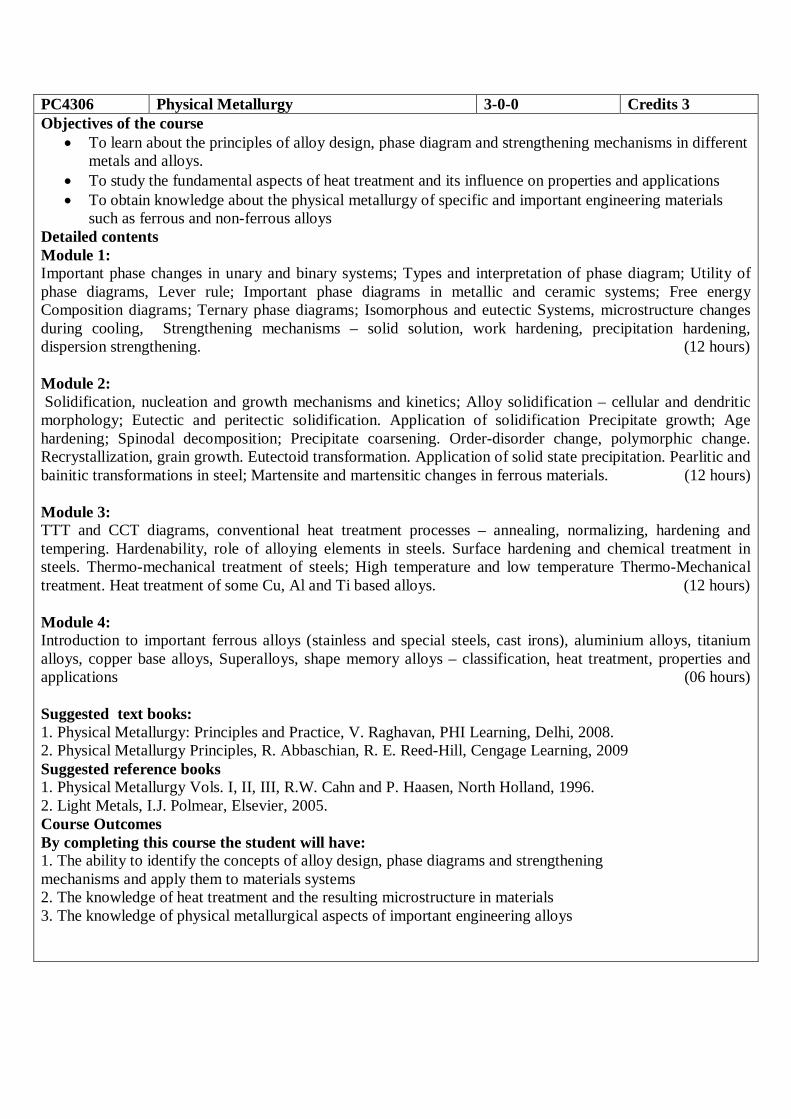
PC4306 Physical Metallurgy 3-0-0 Credits 3 Objectives of the course

• To learn about the principles of alloy design, phase diagram and strengthening mechanisms in different metals and alloys.

• To study the fundamental aspects of heat treatment and its influence on properties and applications • To obtain knowledge about the physical metallurgy of specific and important engineering materials

such as ferrous and non-ferrous alloys Detailed contents Module 1: Important phase changes in unary and binary systems; Types and interpretation of phase diagram; Utility of phase diagrams, Lever rule; Important phase diagrams in metallic and ceramic systems; Free energy Composition diagrams; Ternary phase diagrams; Isomorphous and eutectic Systems, microstructure changes during cooling, Strengthening mechanisms – solid solution, work hardening, precipitation hardening, dispersion strengthening. (12 hours) Module 2: Solidification, nucleation and growth mechanisms and kinetics; Alloy solidification – cellular and dendritic morphology; Eutectic and peritectic solidification. Application of solidification Precipitate growth; Age hardening; Spinodal decomposition; Precipitate coarsening. Order-disorder change, polymorphic change. Recrystallization, grain growth. Eutectoid transformation. Application of solid state precipitation. Pearlitic and bainitic transformations in steel; Martensite and martensitic changes in ferrous materials. (12 hours) Module 3: TTT and CCT diagrams, conventional heat treatment processes – annealing, normalizing, hardening and tempering. Hardenability, role of alloying elements in steels. Surface hardening and chemical treatment in steels. Thermo-mechanical treatment of steels; High temperature and low temperature Thermo-Mechanical treatment. Heat treatment of some Cu, Al and Ti based alloys. (12 hours) Module 4: Introduction to important ferrous alloys (stainless and special steels, cast irons), aluminium alloys, titanium alloys, copper base alloys, Superalloys, shape memory alloys – classification, heat treatment, properties and applications (06 hours) Suggested text books: 1. Physical Metallurgy: Principles and Practice, V. Raghavan, PHI Learning, Delhi, 2008. 2. Physical Metallurgy Principles, R. Abbaschian, R. E. Reed-Hill, Cengage Learning, 2009 Suggested reference books 1. Physical Metallurgy Vols. I, II, III, R.W. Cahn and P. Haasen, North Holland, 1996. 2. Light Metals, I.J. Polmear, Elsevier, 2005. Course Outcomes By completing this course the student will have: 1. The ability to identify the concepts of alloy design, phase diagrams and strengthening mechanisms and apply them to materials systems 2. The knowledge of heat treatment and the resulting microstructure in materials 3. The knowledge of physical metallurgical aspects of important engineering alloys

Lecture No.

1. Introduction to phase transformation, Important phase changes in unary and binary systems

2. Types and interpretation of phase diagram; Utility of phase diagrams, Isomorphous and eutectic Systems

3. Lever rule; Important phase diagrams in metallic and ceramic systems 4. Ternary phase diagrams 5. Microstructure changes during cooling 6. Free energy Composition diagrams 7. Strengthening mechanisms (Basics) 8. Details on solid solution, work hardening, precipitation hardening, dispersion

strengthening 9. Solidification, nucleation and growth mechanisms and kinetics (In pure metals) 10. Alloy solidification – cellular and dendritic morphology (In alloys) 11. Eutectic and peritectic solidification 12. Recrystallization, grain growth 13. Idea on Solid-state phase transformation (diffusion based transformation);

Precipitate growth 14. Age hardening 15. Spinodal decomposition; Order-disorder change 16. Precipitate coarsening, polymorphic change 17. Eutectoid transformation, Pearlitic and bainitic transformations in steel 18. Diffusionless phase transformation; Martensite and martensitic changes in

ferrous materials 19. Basics of heat treatment; TTT and CCT diagrams 20. Conventional heat treatment processes – annealing, normalizing, hardening and

tempering. 21. Hardenability 22. Effect of alloying elements in steels 23. Surface hardening and chemical treatment in steels 24. Thermo-mechanical treatment of steels; High temperature and low temperature

Thermo-Mechanical treatment 25. Heat treatment of some Cu, Al and Ti based alloys (Part -1) 26. Heat treatment of some Cu, Al and Ti based alloys (Part -2) 27. Introduction to important ferrous alloys (stainless steels) 28. Introduction to important ferrous alloys (Special steels) 29. Introduction to important ferrous alloys (Cast irons) 30. Aluminium alloys, Copper base alloys (classification, heat treatment, properties

and applications) 31. Superalloys, Titanium alloys (classification, heat treatment, properties and

applications) 32. Shape memory alloys – classification, heat treatment, properties and applications

Module – 1

Lecture – 1

(Introduction to phase transformation, important phase changes in unary and binary systems)

1.1 Phases

For the understanding of phase diagrams, it is essential to understand the concept of a phase.

A phase may be defined as a homogeneous portion of a system that has uniform physical and

chemical characteristics. Every pure material is considered to be a phase; so also is every

solid, liquid, and gaseous solution. For example, the sugar–water syrup solution just

discussed is one phase, and solid sugar is another. Each has different physical properties (one

is a liquid, the other is a solid); furthermore, each is different chemically (i.e., has a different

chemical composition); one is virtually pure sugar, the other is a solution of and if more than

one phase is present in a given system, each will have its own distinct properties, and a

boundary separating the phases will exist across which there will be a discontinuous and

abrupt change in physical and/or chemical characteristics. When two phases are present in a

system, it is not necessary that there be a difference in both physical and chemical properties;

a disparity in one or the other set of properties is sufficient. When water and ice are present in

a container, two separate phases exist; they are physically dissimilar (one is a solid, the other

is a liquid) but identical in chemical makeup. Also, when a substance can exist in two or

more polymorphic forms (e.g., having both FCC and BCC structures), each of these

structures is a separate phase because their respective physical characteristics differ.

1.2 Phase diagram Much of the information about the control of the phase structure of a particular system is

conveniently and concisely displayed in what is called a phase diagram, also often termed an

equilibrium diagram. Now, there are three externally controllable parameters that will affect

phase structure—viz. temperature, pressure, and composition and phase diagrams are

constructed when various combinations of these parameters are plotted against one another.

1.3 One - Component (Unary) Phase diagrams Perhaps the simplest and easiest type of phase diagram to understand is that for a one-

component system, in which composition is held constant (i.e., the phase diagram is for a

pure substance); this means that pressure and temperature are the variables. This one-

component phase diagram (or unary phase diagram) sometimes also called a pressure–

temperature (or P–T) diagram is represented as a two-dimensional plot of pressure (ordinate

or vertical axis) versus temperature (abscissa, or horizontal axis). Most often, the pressure

axis is scaled logarithmically. We illustrate this type of phase diagram and demonstrate its

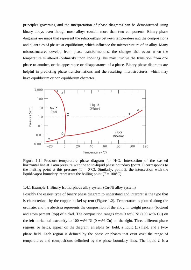
interpretation using as an example the one for, which is shown in Figure 1.1. Here it may be

noted that regions for three different phases—solid, liquid, and vapor—are delineated on the

plot. Each of the phases will exist under equilibrium conditions over the temperature–

pressure ranges of its corresponding area. Furthermore, the three curves shown on the plot

(labelled aO, bO, and cO) are phase boundaries; at any point on one of these curves, the two

phases on either side of the curve are in equilibrium (or coexist) with one another. That is,

equilibrium between solid and vapour phases is along curve aO—likewise for the solid-

liquid, curve bO, and the liquid vapor, curve cO. Also, upon crossing a boundary (as

temperature and/or pressure is altered), one phase transforms to another. For example, at one

atmosphere pressure, during heating the solid phase transforms to the liquid phase (i.e.,

melting occurs) at the point labelled 2 on Figure 1.1 (i.e., the intersection of the dashed

horizontal line with the solid-liquid phase boundary); this point corresponds to a temperature

of 0°C. Of course, the reverse transformation (liquid-to-solid or solidification) takes place at

the same point upon cooling. Similarly, at the intersection of the dashed line with the liquid-

vapor phase boundary [point 3 (Figure 1.1), at 100°C] the liquid transforms to the vapor

phase (or vaporizes) upon heating; As may also be noted from Figure 1.1, all three of the

phase boundary curves intersect at a common point, which is labelled O (and for this system,

at a temperature of 273.16 K and a pressure of atm). This means that at this point only, all of

the solid, liquid, and vapor phases are simultaneously in equilibrium with one another.

Appropriately, this, and any other point on a P–T phase diagram where three phases are in

equilibrium, is called a triple point; sometimes it is also termed an invariant point in as much

as its position is distinct, or fixed by definite values of pressure and temperature. Any

deviation from this point by a change of temperature and/or pressure will cause at least one of

the phases to disappear.

1.4 Binary Phase Diagrams Another type of extremely common phase diagram is one in which temperature and

composition are variable parameters, and pressure is held constant, normally 1 atm. There are

several different varieties; in the present discussion, we will concern ourselves with binary

alloys—those that contain two components. If more than two components are present, phase

diagrams become extremely complicated and difficult to represent. An explanation of the

principles governing and the interpretation of phase diagrams can be demonstrated using

binary alloys even though most alloys contain more than two components. Binary phase

diagrams are maps that represent the relationships between temperature and the compositions

and quantities of phases at equilibrium, which influence the microstructure of an alloy. Many

microstructures develop from phase transformations, the changes that occur when the

temperature is altered (ordinarily upon cooling).This may involve the transition from one

phase to another, or the appearance or disappearance of a phase. Binary phase diagrams are

helpful in predicting phase transformations and the resulting microstructures, which may

have equilibrium or non equilibrium character.

Figure 1.1: Pressure–temperature phase diagram for H2O. Intersection of the dashed horizontal line at 1 atm pressure with the solid-liquid phase boundary (point 2) corresponds to the melting point at this pressure (T = 0°C). Similarly, point 3, the intersection with the liquid-vapor boundary, represents the boiling point (T = 100°C).

1.4.1 Example 1: Binary Isomorphous alloy system (Cu-Ni alloy system)

Possibly the easiest type of binary phase diagram to understand and interpret is the type that

is characterized by the copper–nickel system (Figure 1.2). Temperature is plotted along the

ordinate, and the abscissa represents the composition of the alloy, in weight percent (bottom)

and atom percent (top) of nickel. The composition ranges from 0 wt% Ni (100 wt% Cu) on

the left horizontal extremity to 100 wt% Ni (0 wt% Cu) on the right. Three different phase

regions, or fields, appear on the diagram, an alpha (α) field, a liquid (L) field, and a two-

phase field. Each region is defined by the phase or phases that exist over the range of

temperatures and compositions delimited by the phase boundary lines. The liquid L is a

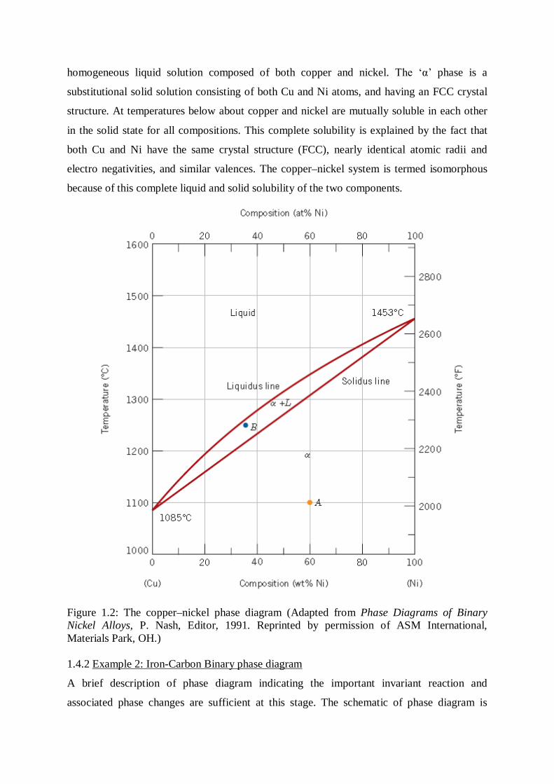
homogeneous liquid solution composed of both copper and nickel. The ‘α’ phase is a

substitutional solid solution consisting of both Cu and Ni atoms, and having an FCC crystal

structure. At temperatures below about copper and nickel are mutually soluble in each other

in the solid state for all compositions. This complete solubility is explained by the fact that

both Cu and Ni have the same crystal structure (FCC), nearly identical atomic radii and

electro negativities, and similar valences. The copper–nickel system is termed isomorphous

because of this complete liquid and solid solubility of the two components.

Figure 1.2: The copper–nickel phase diagram (Adapted from Phase Diagrams of Binary Nickel Alloys, P. Nash, Editor, 1991. Reprinted by permission of ASM International, Materials Park, OH.) 1.4.2 Example 2: Iron-Carbon Binary phase diagram

A brief description of phase diagram indicating the important invariant reaction and

associated phase changes are sufficient at this stage. The schematic of phase diagram is

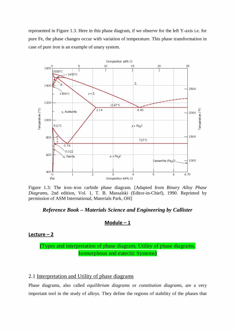
represented in Figure 1.3. Here in this phase diagram, if we observe for the left Y-axis i.e. for

pure Fe, the phase changes occur with variation of temperature. This phase transformation in

case of pure iron is an example of unary system.

Figure 1.3: The iron–iron carbide phase diagram. [Adapted from Binary Alloy Phase Diagrams, 2nd edition, Vol. 1, T. B. Massalski (Editor-in-Chief), 1990. Reprinted by permission of ASM International, Materials Park, OH]

Reference Book – Materials Science and Engineering by Callister

Module – 1

Lecture – 2

(Types and interpretation of phase diagram; Utility of phase diagrams, Isomorphous and eutectic Systems)

2.1 Interpretation and Utility of phase diagrams Phase diagrams, also called equilibrium diagrams or constitution diagrams, are a very

important tool in the study of alloys. They define the regions of stability of the phases that

can occur in an alloy system under the condition of constant pressure (atmospheric). The

coordinates of these diagrams are temperature (ordinate) and composition (abscissa). Notice

that the expression “alloy system” is used to mean all the possible alloys that can be formed

from a given set of components. This use of the word system differs from the thermodynamic

definition of a system, which refers to a single isolated body of matter. An alloy of one

composition is representative of a thermodynamic system, while an alloy system signifies all

compositions considered together.

The interrelationships between the phases, the temperature, and the composition in an alloy

system are shown by phase diagrams only under equilibrium conditions. These diagrams do

not apply directly to metals not at equilibrium. A metal quenched (cooled rapidly) from a

higher temperature to a lower one (for example, room temperature) may possess phases or

metastable phase and compositions that are more characteristic of the higher temperature than

they are of the lower temperature. In time, as a result of thermally activated atomic motion,

the quenched specimen may approach its equilibrium low temperature state. If and when this

occurs, the phase relationships in the specimen will conform to the equilibrium diagram. In

other words, the phase diagram at any given temperature gives us the proper picture only if

sufficient time is allowed for the metal to come to equilibrium.

2.2 Isomorphous Alloy system The Cu-Ni isomorphous alloy system is already discussed in section 1.4.1. The detailed

explanation to this Cu-Ni alloy system is described here and is represented in Figure 2.1. The

area in the figure above the line marked “liquidus” corresponds to the region of stability of

the liquid phase, and the area below the solidus line represents the stable region for the solid

phase. Between the liquidus and solidus lines is a two-phase area where both phases can

coexist. A set of coordinates—a temperature and a composition—is associated with each

point. By dropping a vertical line from point x until it touches the axis of abscissa, we find the

composition 20 percent Cu. Similarly, a horizontal line through the same point meets the

ordinate axis at 500°C. The Point x signifies an alloy of 20 percent Cu and 80 percent Ni at a

temperature of 500°C. The fact that the given point lies in the region below the solidus line

tells us that the equilibrium state of this alloy is the solid phase. The structure implied is,

therefore, one of solid solution crystals, and each crystal will have the same homogeneous

composition (20 percent Cu and 80 percent Ni). Under the microscope, such a structure will

be identical to a pure metal in appearance. In other respects, however, a metal of the given

composition will have different properties. It should be stronger and have a higher resistivity

than either pure metal, or it will also have a different surface sheen or color. The point, y,

which falls inside the two-phase region, the area bounded by the liquidus and solidus lines.

The indicated temperature in this case is 1200°C, while the composition is 70 percent Cu and

30 percent Ni. This 70 to 30 ratio of the components represents the average composition of

the alloy as a whole. It should be remembered that we are now dealing with a mixture of

phases (liquid plus solid) and that neither possesses the average composition. To determine

the compositions of the liquid and the solid in the given phase mixture, it is only necessary to

extend a horizontal line (called a tie line) through point y until it intersects the liquidus and

solidus lines. These intersections give the desired compositions. In Fig. 2.1, the intersections

are at points m and n, respectively. A vertical line dropped from point m to the abscissa axis

gives 62 percent Cu, which is the composition of the solid phase. In the same manner, a

vertical line dropped from point n shows that the composition of the liquid is 78 percent Cu.

Figure 2.1: The copper-nickel phase diagram

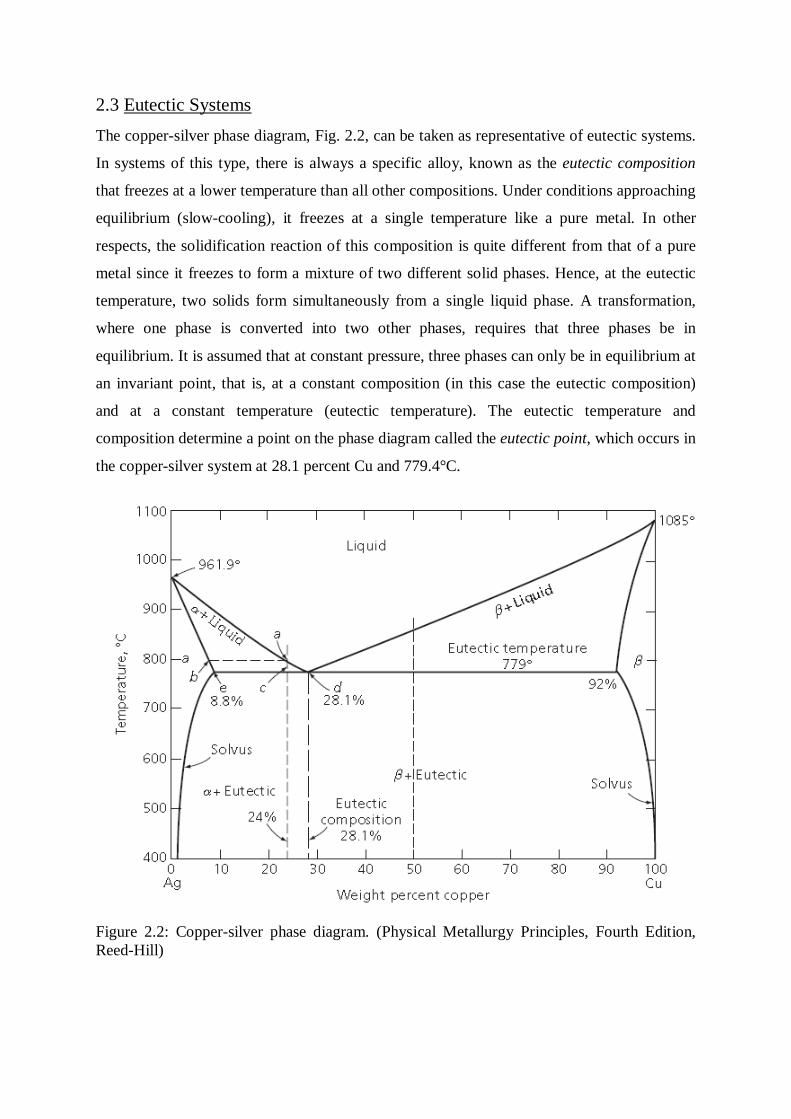
2.3 Eutectic Systems The copper-silver phase diagram, Fig. 2.2, can be taken as representative of eutectic systems.

In systems of this type, there is always a specific alloy, known as the eutectic composition

that freezes at a lower temperature than all other compositions. Under conditions approaching

equilibrium (slow-cooling), it freezes at a single temperature like a pure metal. In other

respects, the solidification reaction of this composition is quite different from that of a pure

metal since it freezes to form a mixture of two different solid phases. Hence, at the eutectic

temperature, two solids form simultaneously from a single liquid phase. A transformation,

where one phase is converted into two other phases, requires that three phases be in

equilibrium. It is assumed that at constant pressure, three phases can only be in equilibrium at

an invariant point, that is, at a constant composition (in this case the eutectic composition)

and at a constant temperature (eutectic temperature). The eutectic temperature and

composition determine a point on the phase diagram called the eutectic point, which occurs in

the copper-silver system at 28.1 percent Cu and 779.4°C.

Figure 2.2: Copper-silver phase diagram. (Physical Metallurgy Principles, Fourth Edition, Reed-Hill)

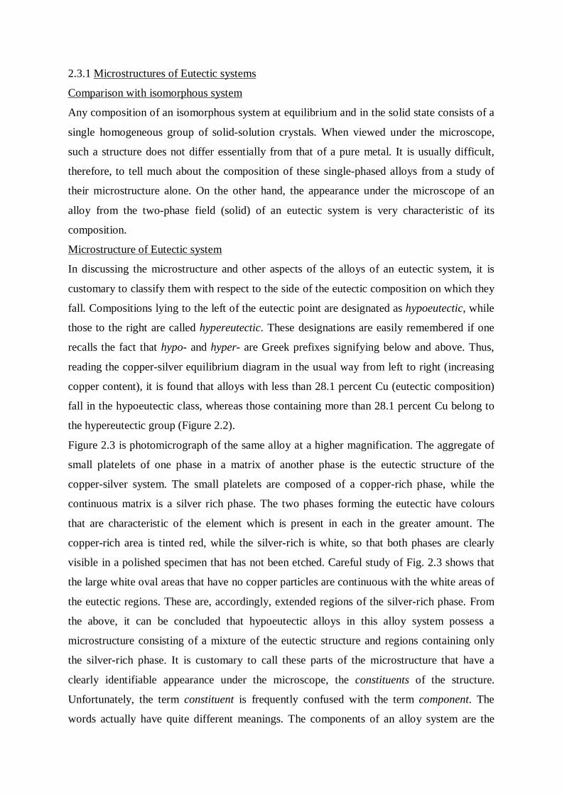
2.3.1 Microstructures of Eutectic systems

Comparison with isomorphous system

Any composition of an isomorphous system at equilibrium and in the solid state consists of a

single homogeneous group of solid-solution crystals. When viewed under the microscope,

such a structure does not differ essentially from that of a pure metal. It is usually difficult,

therefore, to tell much about the composition of these single-phased alloys from a study of

their microstructure alone. On the other hand, the appearance under the microscope of an

alloy from the two-phase field (solid) of an eutectic system is very characteristic of its

composition.

Microstructure of Eutectic system

In discussing the microstructure and other aspects of the alloys of an eutectic system, it is

customary to classify them with respect to the side of the eutectic composition on which they

fall. Compositions lying to the left of the eutectic point are designated as hypoeutectic, while

those to the right are called hypereutectic. These designations are easily remembered if one

recalls the fact that hypo- and hyper- are Greek prefixes signifying below and above. Thus,

reading the copper-silver equilibrium diagram in the usual way from left to right (increasing

copper content), it is found that alloys with less than 28.1 percent Cu (eutectic composition)

fall in the hypoeutectic class, whereas those containing more than 28.1 percent Cu belong to

the hypereutectic group (Figure 2.2).

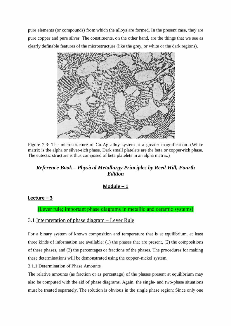
Figure 2.3 is photomicrograph of the same alloy at a higher magnification. The aggregate of

small platelets of one phase in a matrix of another phase is the eutectic structure of the

copper-silver system. The small platelets are composed of a copper-rich phase, while the

continuous matrix is a silver rich phase. The two phases forming the eutectic have colours

that are characteristic of the element which is present in each in the greater amount. The

copper-rich area is tinted red, while the silver-rich is white, so that both phases are clearly

visible in a polished specimen that has not been etched. Careful study of Fig. 2.3 shows that

the large white oval areas that have no copper particles are continuous with the white areas of

the eutectic regions. These are, accordingly, extended regions of the silver-rich phase. From

the above, it can be concluded that hypoeutectic alloys in this alloy system possess a

microstructure consisting of a mixture of the eutectic structure and regions containing only

the silver-rich phase. It is customary to call these parts of the microstructure that have a

clearly identifiable appearance under the microscope, the constituents of the structure.

Unfortunately, the term constituent is frequently confused with the term component. The

words actually have quite different meanings. The components of an alloy system are the

pure elements (or compounds) from which the alloys are formed. In the present case, they are

pure copper and pure silver. The constituents, on the other hand, are the things that we see as

clearly definable features of the microstructure (like the grey, or white or the dark regions).

Figure 2.3: The microstructure of Cu-Ag alloy system at a greater magnification. (White matrix is the alpha or silver-rich phase. Dark small platelets are the beta or copper-rich phase. The eutectic structure is thus composed of beta platelets in an alpha matrix.)

Reference Book – Physical Metallurgy Principles by Reed-Hill, Fourth Edition

Module – 1

Lecture – 3

(Lever rule; important phase diagrams in metallic and ceramic systems)

3.1 Interpretation of phase diagram – Lever Rule

For a binary system of known composition and temperature that is at equilibrium, at least

three kinds of information are available: (1) the phases that are present, (2) the compositions

of these phases, and (3) the percentages or fractions of the phases. The procedures for making

these determinations will be demonstrated using the copper–nickel system.

3.1.1 Determination of Phase Amounts

The relative amounts (as fraction or as percentage) of the phases present at equilibrium may

also be computed with the aid of phase diagrams. Again, the single- and two-phase situations

must be treated separately. The solution is obvious in the single phase region: Since only one

phase is present, the alloy is composed entirely of that phase; that is, the phase fraction is 1.0

or, alternatively, the percentage is 100%. If the composition and temperature position is

located within a two-phase region, things are more complex. The tie line must be utilized in

conjunction with a procedure that is often called the lever rule (or the inverse lever rule),

which is applied as follows:

1. The tie line is constructed across the two-phase region at the temperature of the alloy.

2. The overall alloy composition is located on the tie line.

3. The fraction of one phase is computed by taking the length of tie line from the overall alloy

composition to the phase boundary for the other phase, and dividing by the total tie line

length.

4. The fraction of the other phase is determined in the same manner.

5. If phase percentages are desired, each phase fraction is multiplied by 100. When the

composition axis is scaled in weight percent, the phase fractions computed using the lever

rule are mass fractions—the mass (or weight) of a specific phase divided by the total alloy

mass (or weight). The mass of each phase is computed from the product of each phase

fraction and the total alloy mass.

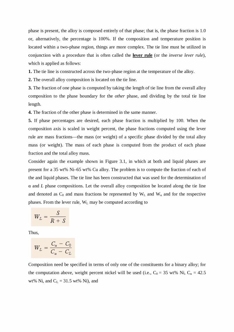
Consider again the example shown in Figure 3.1, in which at both and liquid phases are

present for a 35 wt% Ni–65 wt% Cu alloy. The problem is to compute the fraction of each of

the and liquid phases. The tie line has been constructed that was used for the determination of

α and L phase compositions. Let the overall alloy composition be located along the tie line

and denoted as C0 and mass fractions be represented by WL and Wα and for the respective

phases. From the lever rule, WL may be computed according to

Thus,

Composition need be specified in terms of only one of the constituents for a binary alloy; for

the computation above, weight percent nickel will be used (i.e., C0 = 35 wt% Ni, Cα = 42.5

wt% Ni, and CL = 31.5 wt% Ni), and

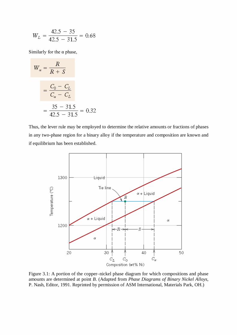
Similarly for the α phase,

Thus, the lever rule may be employed to determine the relative amounts or fractions of phases

in any two-phase region for a binary alloy if the temperature and composition are known and

if equilibrium has been established.

Figure 3.1: A portion of the copper–nickel phase diagram for which compositions and phase amounts are determined at point B. (Adapted from Phase Diagrams of Binary Nickel Alloys, P. Nash, Editor, 1991. Reprinted by permission of ASM International, Materials Park, OH.)

3.2 Important phase diagrams in metallic and ceramic systems 3.2.1 Examples of Metallic system Some common phase diagrams of metallic system are already discussed in the previous

section. These are Cu-Ni, Fe-C, Pb-Sn etc. The eutectic Pb-Sn alloy system is represented in

Figure 3.2 and the description of the reaction taking place in this alloy system is similar to

that mentioned in Section 2.3.

Figure 3.2: Pb-Sn phase diagram

3.2.1 Examples of Non-metallic system

Some common examples are SiO2-Al2O3, Al2O3-Cr2O3 etc. These are represented in Figure

3.3 and 3.4 respectively.

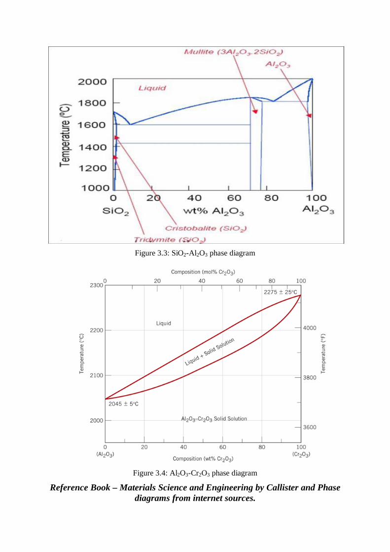
Figure 3.3: SiO2-Al2O3 phase diagram

Figure 3.4: Al2O3-Cr2O3 phase diagram

Reference Book – Materials Science and Engineering by Callister and Phase diagrams from internet sources.

Module – 1

Lecture – 4

(Ternary phase diagrams)

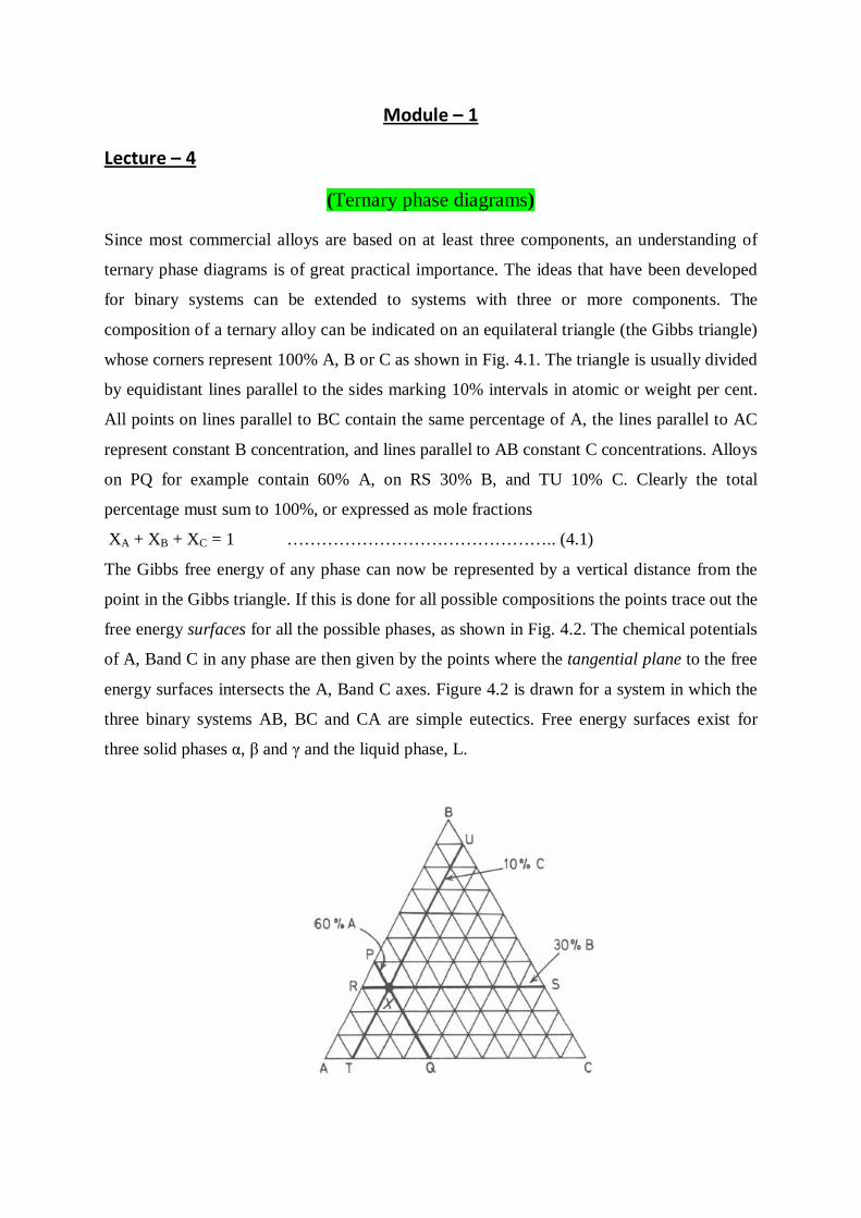
Since most commercial alloys are based on at least three components, an understanding of

ternary phase diagrams is of great practical importance. The ideas that have been developed

for binary systems can be extended to systems with three or more components. The

composition of a ternary alloy can be indicated on an equilateral triangle (the Gibbs triangle)

whose corners represent 100% A, B or C as shown in Fig. 4.1. The triangle is usually divided

by equidistant lines parallel to the sides marking 10% intervals in atomic or weight per cent.

All points on lines parallel to BC contain the same percentage of A, the lines parallel to AC

represent constant B concentration, and lines parallel to AB constant C concentrations. Alloys

on PQ for example contain 60% A, on RS 30% B, and TU 10% C. Clearly the total

percentage must sum to 100%, or expressed as mole fractions

XA + XB + XC = 1 ……………………………………….. (4.1)

The Gibbs free energy of any phase can now be represented by a vertical distance from the

point in the Gibbs triangle. If this is done for all possible compositions the points trace out the

free energy surfaces for all the possible phases, as shown in Fig. 4.2. The chemical potentials

of A, Band C in any phase are then given by the points where the tangential plane to the free

energy surfaces intersects the A, Band C axes. Figure 4.2 is drawn for a system in which the

three binary systems AB, BC and CA are simple eutectics. Free energy surfaces exist for

three solid phases α, β and γ and the liquid phase, L.

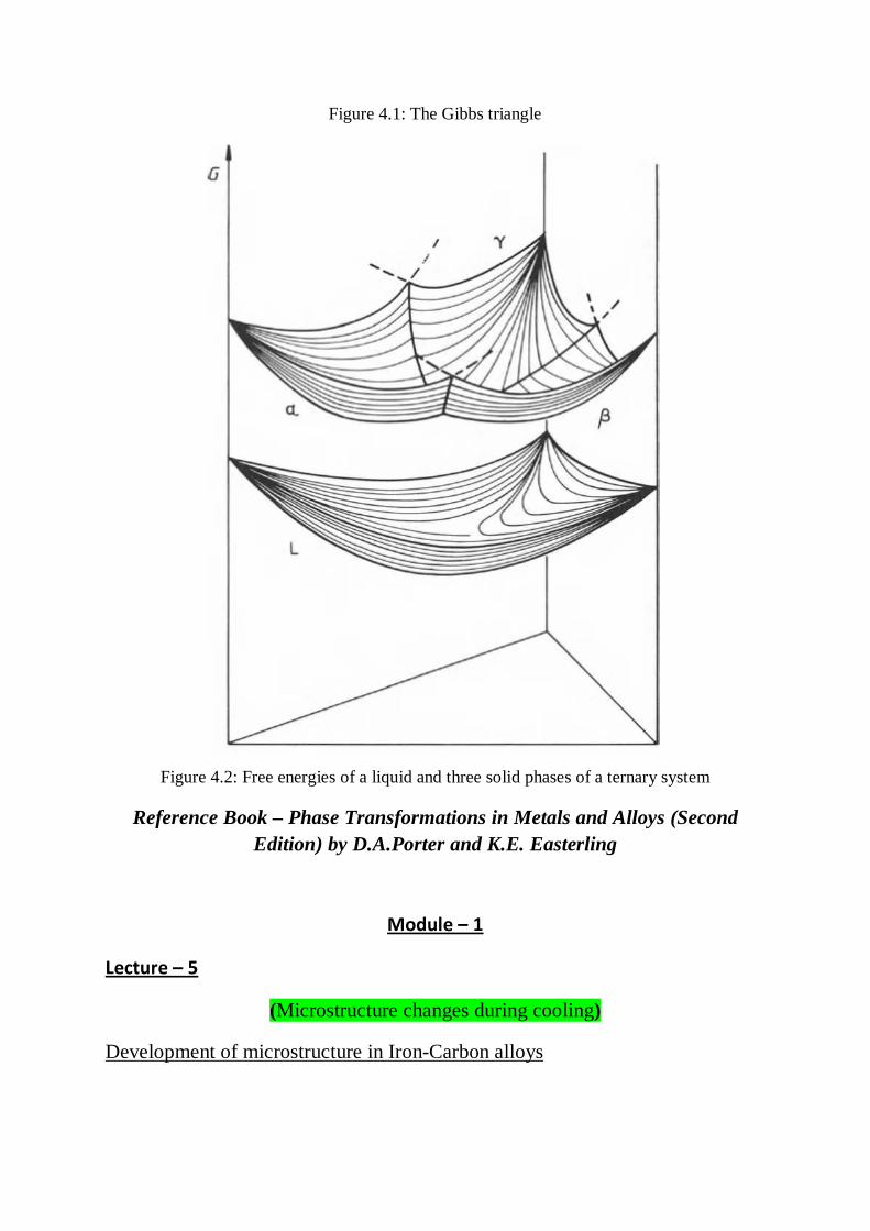
Figure 4.1: The Gibbs triangle

Figure 4.2: Free energies of a liquid and three solid phases of a ternary system

Reference Book – Phase Transformations in Metals and Alloys (Second Edition) by D.A.Porter and K.E. Easterling

Module – 1

Lecture – 5

(Microstructure changes during cooling)

Development of microstructure in Iron-Carbon alloys

Phase changes that occur upon passing from the region into the Fe3C phase field are

relatively complex and similar to those described for the eutectic systems. Consider, for

example, an alloy of eutectoid composition (0.76 wt% C) as it is cooled from a temperature

within the phase region, say, 800°C—that is, beginning at point a in Figure 5.1 and moving

down the vertical line xx’. Initially, the alloy is composed entirely of the austenite phase

having a composition of 0.76 wt% C and corresponding microstructure, also indicated in

Figure 5.1. As the alloy is cooled, there will occur no changes until the eutectoid temperature

is reached. Upon crossing this temperature to point b, the austenite transforms. The

microstructure for this eutectoid steel that is slowly cooled through the eutectoid temperature

consists of alternating layers or lamellae of the two phases (and Fe3C) that form

simultaneously during the transformation. In this case, the relative layer thickness is

approximately 8 to 1. This microstructure, represented schematically in Figure 5.1, point b, is

called pearlite because it has the appearance of mother of pearl when viewed under the

microscope at low magnifications. Figure 5.2 is a photomicrograph of eutectoid steel showing

the pearlite. The pearlite exists as grains, often termed “colonies”; within each colony the

layers are oriented in essentially the same direction, which varies from one colony to another.

The thick light layers are the ferrite phase, and the cementite phase appears as thin lamellae

most of which appear dark. Many cementite layers are so thin that adjacent phase boundaries

are so close together that they are indistinguishable at this magnification, and, therefore,

appear dark. Mechanically, pearlite has properties intermediate between the soft, ductile

ferrite and the hard, brittle cementite. The alternating α and Fe3C layers in pearlite form as

such for the same reason that the eutectic structure forms because the composition of the

parent phase [in this case austenite (0.76 wt% C)] is different from either of the product

phases [ferrite (0.022 wt% C) and cementite (6.7 wt% C)], and the phase transformation

requires that there be a redistribution of the carbon by diffusion. Figure 5.3 illustrates

schematically microstructural changes that accompany this eutectoid reaction; here the

directions of carbon diffusion are indicated by arrows. Carbon atoms diffuse away from the

0.022 wt% ferrite regions and to the 6.7 wt% cementite layers, as the pearlite extends from

the grain boundary into the unreacted austenite grain. The layered pearlite forms because

carbon atoms need diffuse only minimal distances with the formation of this structure.

Furthermore, subsequent cooling of the pearlite from point b in Figure 5.1 will produce

relatively insignificant microstructural changes.

Figure 5.1: Schematic representations of the microstructures for an iron–carbon alloy of eutectoid composition (0.76 wt% C) above and below the eutectoid temperature.

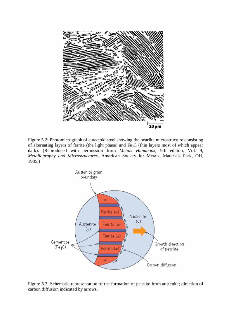
Figure 5.2: Photomicrograph of eutectoid steel showing the pearlite microstructure consisting of alternating layers of ferrite (the light phase) and Fe3C (thin layers most of which appear dark). (Reproduced with permission from Metals Handbook, 9th edition, Vol. 9, Metallography and Microstructures, American Society for Metals, Materials Park, OH, 1985.)

Figure 5.3: Schematic representation of the formation of pearlite from austenite; direction of carbon diffusion indicated by arrows.

Reference Book – Materials Science and Engineering by Callister

Module – 1

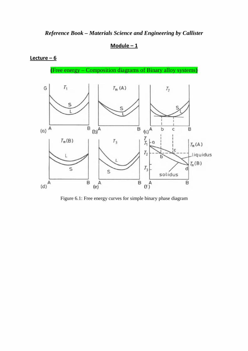
Lecture – 6

(Free energy – Composition diagrams of Binary alloy systems)

Figure 6.1: Free energy curves for simple binary phase diagram

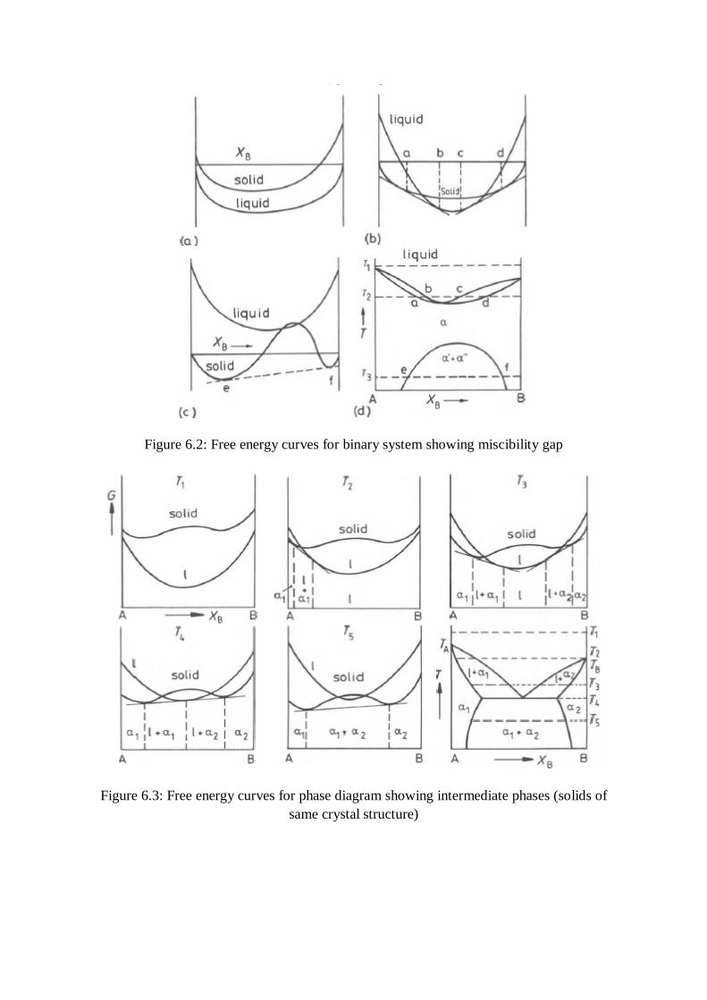
Figure 6.2: Free energy curves for binary system showing miscibility gap

Figure 6.3: Free energy curves for phase diagram showing intermediate phases (solids of same crystal structure)

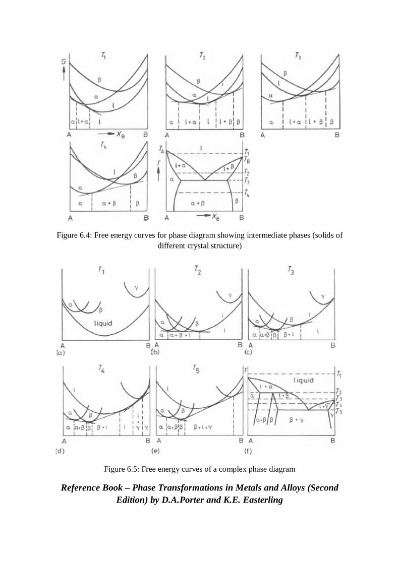
Figure 6.4: Free energy curves for phase diagram showing intermediate phases (solids of different crystal structure)

Figure 6.5: Free energy curves of a complex phase diagram

Reference Book – Phase Transformations in Metals and Alloys (Second Edition) by D.A.Porter and K.E. Easterling

Module – 1

Lecture – 7

(Strengthening mechanisms - Basics)

Metallurgical and materials engineers are often called on to design alloys having high

strengths yet some ductility and toughness; ordinarily, ductility is sacrificed when an alloy is

strengthened. Several hardening techniques are at the disposal of an engineer, and frequently

alloy selection depends on the capacity of a material to be tailored with the mechanical

characteristics required for a particular application. Important to the understanding of

strengthening mechanisms is the relation between dislocation motion and mechanical

behaviour of metals. Because macroscopic plastic deformation corresponds to the motion of

large numbers of dislocations, the ability of a metal to plastically deform depends on the

ability of dislocations to move. Since hardness and strength (both yield and tensile) are

related to the ease with which plastic deformation can be made to occur, by reducing the

mobility of dislocations, the mechanical strength may be enhanced; that is, greater

mechanical forces will be required to initiate plastic deformation. In contrast, the more

unconstrained the dislocation motion, the greater is the facility with which a metal may

deform, and the softer and weaker it becomes. Virtually all strengthening techniques rely on

this simple principle: restricting or hindering dislocation motion renders a material harder

and stronger.

Module – 1

Lecture – 8.

(Details on solid solution, work hardening, precipitation hardening, dispersion strengthening)

Solid solution strengthening

One technique to strengthen and harden metals is alloying with impurity atoms that go into

either substitutional or interstitial solid solution. Accordingly, this is called solid-solution

strengthening. High-purity metals are almost always softer and weaker than alloys

composed of the same base metal. Increasing the concentration of the impurity results in an

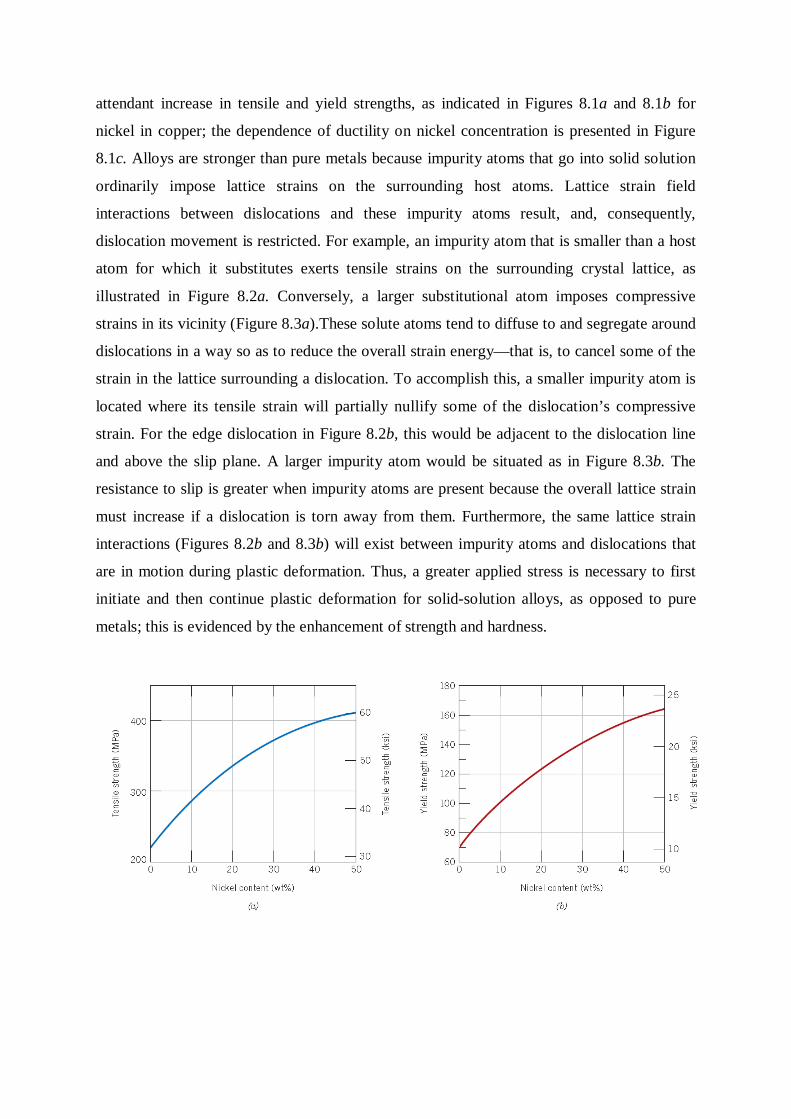
attendant increase in tensile and yield strengths, as indicated in Figures 8.1a and 8.1b for

nickel in copper; the dependence of ductility on nickel concentration is presented in Figure

8.1c. Alloys are stronger than pure metals because impurity atoms that go into solid solution

ordinarily impose lattice strains on the surrounding host atoms. Lattice strain field

interactions between dislocations and these impurity atoms result, and, consequently,

dislocation movement is restricted. For example, an impurity atom that is smaller than a host

atom for which it substitutes exerts tensile strains on the surrounding crystal lattice, as

illustrated in Figure 8.2a. Conversely, a larger substitutional atom imposes compressive

strains in its vicinity (Figure 8.3a).These solute atoms tend to diffuse to and segregate around

dislocations in a way so as to reduce the overall strain energy—that is, to cancel some of the

strain in the lattice surrounding a dislocation. To accomplish this, a smaller impurity atom is

located where its tensile strain will partially nullify some of the dislocation’s compressive

strain. For the edge dislocation in Figure 8.2b, this would be adjacent to the dislocation line

and above the slip plane. A larger impurity atom would be situated as in Figure 8.3b. The

resistance to slip is greater when impurity atoms are present because the overall lattice strain

must increase if a dislocation is torn away from them. Furthermore, the same lattice strain

interactions (Figures 8.2b and 8.3b) will exist between impurity atoms and dislocations that

are in motion during plastic deformation. Thus, a greater applied stress is necessary to first

initiate and then continue plastic deformation for solid-solution alloys, as opposed to pure

metals; this is evidenced by the enhancement of strength and hardness.

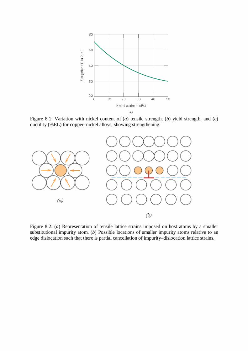
Figure 8.1: Variation with nickel content of (a) tensile strength, (b) yield strength, and (c) ductility (%EL) for copper–nickel alloys, showing strengthening.

Figure 8.2: (a) Representation of tensile lattice strains imposed on host atoms by a smaller substitutional impurity atom. (b) Possible locations of smaller impurity atoms relative to an edge dislocation such that there is partial cancellation of impurity–dislocation lattice strains.

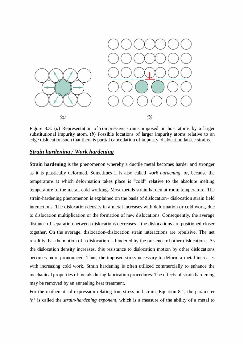
Figure 8.3: (a) Representation of compressive strains imposed on host atoms by a larger substitutional impurity atom. (b) Possible locations of larger impurity atoms relative to an edge dislocation such that there is partial cancellation of impurity–dislocation lattice strains. Strain hardening / Work hardening Strain hardening is the phenomenon whereby a ductile metal becomes harder and stronger

as it is plastically deformed. Sometimes it is also called work hardening, or, because the

temperature at which deformation takes place is “cold” relative to the absolute melting

temperature of the metal, cold working. Most metals strain harden at room temperature. The

strain-hardening phenomenon is explained on the basis of dislocation– dislocation strain field

interactions. The dislocation density in a metal increases with deformation or cold work, due

to dislocation multiplication or the formation of new dislocations. Consequently, the average

distance of separation between dislocations decreases—the dislocations are positioned closer

together. On the average, dislocation–dislocation strain interactions are repulsive. The net

result is that the motion of a dislocation is hindered by the presence of other dislocations. As

the dislocation density increases, this resistance to dislocation motion by other dislocations

becomes more pronounced. Thus, the imposed stress necessary to deform a metal increases

with increasing cold work. Strain hardening is often utilized commercially to enhance the

mechanical properties of metals during fabrication procedures. The effects of strain hardening

may be removed by an annealing heat treatment.

For the mathematical expression relating true stress and strain, Equation 8.1, the parameter

‘n’ is called the strain-hardening exponent, which is a measure of the ability of a metal to

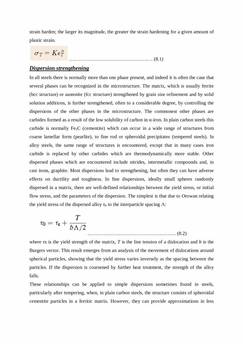
strain harden; the larger its magnitude, the greater the strain hardening for a given amount of

plastic strain.

…………………………………………… (8.1)

Dispersion strengthening In all steels there is normally more than one phase present, and indeed it is often the case that

several phases can be recognized in the microstructure. The matrix, which is usually ferrite

(bcc structure) or austenite (fcc structure) strengthened by grain size refinement and by solid

solution additions, is further strengthened, often to a considerable degree, by controlling the

dispersions of the other phases in the microstructure. The commonest other phases are

carbides formed as a result of the low solubility of carbon in α-iron. In plain carbon steels this

carbide is normally Fe3C (cementite) which can occur in a wide range of structures from

coarse lamellar form (pearlite), to fine rod or spheroidal precipitates (tempered steels). In

alloy steels, the same range of structures is encountered, except that in many cases iron

carbide is replaced by other carbides which are thermodynamically more stable. Other

dispersed phases which are encountered include nitrides, intermetallic compounds and, in

cast irons, graphite. Most dispersions lead to strengthening, but often they can have adverse

effects on ductility and toughness. In fine dispersions, ideally small spheres randomly

dispersed in a matrix, there are well-defined relationships between the yield stress, or initial

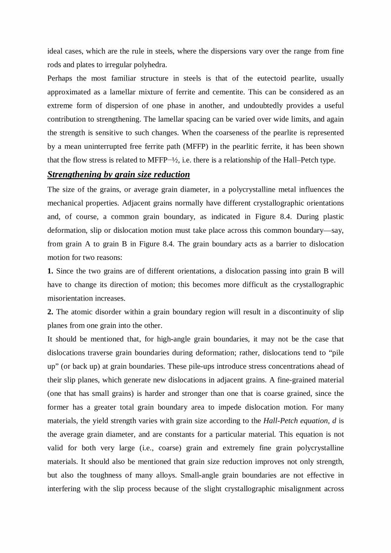
flow stress, and the parameters of the dispersion. The simplest is that due to Orowan relating

the yield stress of the dispersed alloy τ0 to the interparticle spacing Λ:

……………………………………………… (8.2)

where τs is the yield strength of the matrix, T is the line tension of a dislocation and b is the

Burgers vector. This result emerges from an analysis of the movement of dislocations around

spherical particles, showing that the yield stress varies inversely as the spacing between the

particles. If the dispersion is coarsened by further heat treatment, the strength of the alloy

falls.

These relationships can be applied to simple dispersions sometimes found in steels,

particularly after tempering, when, in plain carbon steels, the structure consists of spheroidal

cementite particles in a ferritic matrix. However, they can provide approximations in less

ideal cases, which are the rule in steels, where the dispersions vary over the range from fine

rods and plates to irregular polyhedra.

Perhaps the most familiar structure in steels is that of the eutectoid pearlite, usually

approximated as a lamellar mixture of ferrite and cementite. This can be considered as an

extreme form of dispersion of one phase in another, and undoubtedly provides a useful

contribution to strengthening. The lamellar spacing can be varied over wide limits, and again

the strength is sensitive to such changes. When the coarseness of the pearlite is represented

by a mean uninterrupted free ferrite path (MFFP) in the pearlitic ferrite, it has been shown

that the flow stress is related to MFFP−½, i.e. there is a relationship of the Hall–Petch type.

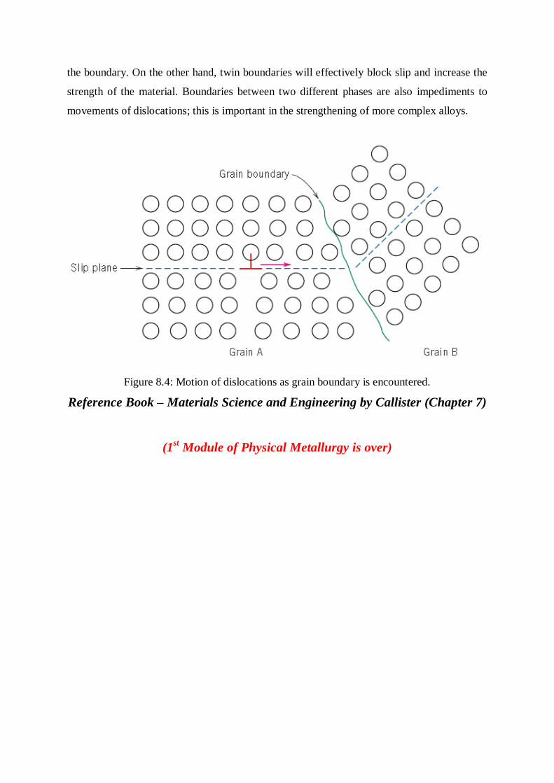
Strengthening by grain size reduction The size of the grains, or average grain diameter, in a polycrystalline metal influences the

mechanical properties. Adjacent grains normally have different crystallographic orientations

and, of course, a common grain boundary, as indicated in Figure 8.4. During plastic

deformation, slip or dislocation motion must take place across this common boundary—say,

from grain A to grain B in Figure 8.4. The grain boundary acts as a barrier to dislocation

motion for two reasons:

1. Since the two grains are of different orientations, a dislocation passing into grain B will

have to change its direction of motion; this becomes more difficult as the crystallographic

misorientation increases.

2. The atomic disorder within a grain boundary region will result in a discontinuity of slip

planes from one grain into the other.

It should be mentioned that, for high-angle grain boundaries, it may not be the case that

dislocations traverse grain boundaries during deformation; rather, dislocations tend to “pile

up” (or back up) at grain boundaries. These pile-ups introduce stress concentrations ahead of

their slip planes, which generate new dislocations in adjacent grains. A fine-grained material

(one that has small grains) is harder and stronger than one that is coarse grained, since the

former has a greater total grain boundary area to impede dislocation motion. For many

materials, the yield strength varies with grain size according to the Hall-Petch equation, d is

the average grain diameter, and are constants for a particular material. This equation is not

valid for both very large (i.e., coarse) grain and extremely fine grain polycrystalline

materials. It should also be mentioned that grain size reduction improves not only strength,

but also the toughness of many alloys. Small-angle grain boundaries are not effective in

interfering with the slip process because of the slight crystallographic misalignment across

the boundary. On the other hand, twin boundaries will effectively block slip and increase the

strength of the material. Boundaries between two different phases are also impediments to

movements of dislocations; this is important in the strengthening of more complex alloys.

Figure 8.4: Motion of dislocations as grain boundary is encountered.

Reference Book – Materials Science and Engineering by Callister (Chapter 7)

(1st Module of Physical Metallurgy is over)