PC237 Lab Manual - Wilfrid Laurier University

PC237 Lab Manual

Hasan Shodiev, Terry Sturtevant1

Winter, 2012

1Physics Lab Instructors

ii

Contents

1 Goals for Physics 237 1

2 Instructions for Physics 237 32.1 Expectations . . . . . . . . . . . . . . . . . . . . . . . . . . . 3

3 Exercise on Reflection and Refraction of Light 73.1 Purpose . . . . . . . . . . . . . . . . . . . . . . . . . . . . . . 73.2 Introduction . . . . . . . . . . . . . . . . . . . . . . . . . . . . 73.3 Theory . . . . . . . . . . . . . . . . . . . . . . . . . . . . . . . 7

3.3.1 Reflection . . . . . . . . . . . . . . . . . . . . . . . . . 73.3.2 Refraction . . . . . . . . . . . . . . . . . . . . . . . . . 8

3.4 Procedure . . . . . . . . . . . . . . . . . . . . . . . . . . . . . 113.4.1 Apparatus . . . . . . . . . . . . . . . . . . . . . . . . . 113.4.2 Preparation . . . . . . . . . . . . . . . . . . . . . . . . 123.4.3 Experimentation . . . . . . . . . . . . . . . . . . . . . 123.4.4 Analysis . . . . . . . . . . . . . . . . . . . . . . . . . . 15

3.5 Bonus . . . . . . . . . . . . . . . . . . . . . . . . . . . . . . . 163.6 Recap . . . . . . . . . . . . . . . . . . . . . . . . . . . . . . . 163.7 Summary . . . . . . . . . . . . . . . . . . . . . . . . . . . . . 163.8 Template . . . . . . . . . . . . . . . . . . . . . . . . . . . . . . 17

4 Exercise on The Brewster Angle 194.1 Purpose . . . . . . . . . . . . . . . . . . . . . . . . . . . . . . 194.2 Theory . . . . . . . . . . . . . . . . . . . . . . . . . . . . . . . 19

4.2.1 Production of Polarized Light . . . . . . . . . . . . . . 204.3 Procedure . . . . . . . . . . . . . . . . . . . . . . . . . . . . . 24

4.3.1 Experimentation . . . . . . . . . . . . . . . . . . . . . 244.3.2 Analysis . . . . . . . . . . . . . . . . . . . . . . . . . . 26

iv CONTENTS

4.4 Recap . . . . . . . . . . . . . . . . . . . . . . . . . . . . . . . 264.5 Summary . . . . . . . . . . . . . . . . . . . . . . . . . . . . . 274.6 Template . . . . . . . . . . . . . . . . . . . . . . . . . . . . . . 28

5 Exercise on the Michelson Interferometer 295.1 Purpose . . . . . . . . . . . . . . . . . . . . . . . . . . . . . . 295.2 Theory . . . . . . . . . . . . . . . . . . . . . . . . . . . . . . . 295.3 Procedure . . . . . . . . . . . . . . . . . . . . . . . . . . . . . 30

5.3.1 Apparatus . . . . . . . . . . . . . . . . . . . . . . . . . 305.3.2 Preparation . . . . . . . . . . . . . . . . . . . . . . . . 305.3.3 Experimentation . . . . . . . . . . . . . . . . . . . . . 305.3.4 Analysis . . . . . . . . . . . . . . . . . . . . . . . . . . 31


6 Exercise on Newton’s Rings 356.1 Purpose . . . . . . . . . . . . . . . . . . . . . . . . . . . . . . 356.2 Theory . . . . . . . . . . . . . . . . . . . . . . . . . . . . . . . 35

6.2.1 Newton’s Rings . . . . . . . . . . . . . . . . . . . . . . 366.3 Procedure . . . . . . . . . . . . . . . . . . . . . . . . . . . . . 39

6.3.1 Preparation . . . . . . . . . . . . . . . . . . . . . . . . 396.3.2 Apparatus . . . . . . . . . . . . . . . . . . . . . . . . . 396.3.3 Experimentation . . . . . . . . . . . . . . . . . . . . . 396.3.4 Analysis . . . . . . . . . . . . . . . . . . . . . . . . . . 40


7 Exercise on Generalized Least Squares Fitting 437.1 Purpose . . . . . . . . . . . . . . . . . . . . . . . . . . . . . . 437.2 Introduction . . . . . . . . . . . . . . . . . . . . . . . . . . . . 437.3 Theory . . . . . . . . . . . . . . . . . . . . . . . . . . . . . . . 43

7.3.1 Non-linear . . . . . . . . . . . . . . . . . . . . . . . . . 437.3.2 Linear . . . . . . . . . . . . . . . . . . . . . . . . . . . 447.3.3 Goodness of fit . . . . . . . . . . . . . . . . . . . . . . 45

7.4 Example . . . . . . . . . . . . . . . . . . . . . . . . . . . . . . 467.5 Procedure . . . . . . . . . . . . . . . . . . . . . . . . . . . . . 54

CONTENTS v

7.5.1 Investigation . . . . . . . . . . . . . . . . . . . . . . . 547.6 Summary . . . . . . . . . . . . . . . . . . . . . . . . . . . . . 567.7 Template . . . . . . . . . . . . . . . . . . . . . . . . . . . . . . 57

8 Thin Lenses 598.1 Purpose . . . . . . . . . . . . . . . . . . . . . . . . . . . . . . 598.2 Introduction . . . . . . . . . . . . . . . . . . . . . . . . . . . . 598.3 Theory . . . . . . . . . . . . . . . . . . . . . . . . . . . . . . . 598.4 Procedure . . . . . . . . . . . . . . . . . . . . . . . . . . . . . 63

8.4.1 Apparatus . . . . . . . . . . . . . . . . . . . . . . . . . 638.4.2 Preparation . . . . . . . . . . . . . . . . . . . . . . . . 638.4.3 Experimentation . . . . . . . . . . . . . . . . . . . . . 638.4.4 Analysis . . . . . . . . . . . . . . . . . . . . . . . . . . 66

8.5 Bonus . . . . . . . . . . . . . . . . . . . . . . . . . . . . . . . 668.6 Summary . . . . . . . . . . . . . . . . . . . . . . . . . . . . . 66

A Aligning the Spectrometer 67A.1 Introduction . . . . . . . . . . . . . . . . . . . . . . . . . . . . 67

A.1.1 Levelling the Spectrometer . . . . . . . . . . . . . . . . 67A.1.2 Telescope Adjustment . . . . . . . . . . . . . . . . . . 68A.1.3 Collimator Alignment . . . . . . . . . . . . . . . . . . . 69

vi CONTENTS

List of Figures

3.1 Reflection of Light at a Mirror . . . . . . . . . . . . . . . . . . 93.2 Virtual Image Produced by a Mirror . . . . . . . . . . . . . . 93.3 Refraction of Light as it Passes from one Medium to Another . 103.4 Refraction of Light Passing Through a Glass Slab . . . . . . . 12

4.1 The Polarization of Light . . . . . . . . . . . . . . . . . . . . . 204.2 Brewster’s Law . . . . . . . . . . . . . . . . . . . . . . . . . . 214.3 Polarization by Successive Reflection . . . . . . . . . . . . . . 234.4 Polarization by Reflection and by Transmission . . . . . . . . 24

6.1 Plano–Convex Lens . . . . . . . . . . . . . . . . . . . . . . . . 376.2 Newton’s Rings Setup . . . . . . . . . . . . . . . . . . . . . . 38

7.1 Plot of Sample Data . . . . . . . . . . . . . . . . . . . . . . . 477.2 Graph of Fit to A+B/x . . . . . . . . . . . . . . . . . . . . . 487.3 Graph of Fit to A+B/x+ C/x2 . . . . . . . . . . . . . . . . 517.4 Graph of Fit to A+B/x+ C/x2 +D/x3 . . . . . . . . . . . . 54

8.1 Light Passing Through a Thin Lens . . . . . . . . . . . . . . . 608.2 Location of Back Focus . . . . . . . . . . . . . . . . . . . . . . 608.3 Focal Plane of a Lens . . . . . . . . . . . . . . . . . . . . . . . 618.4 Front Focal Point . . . . . . . . . . . . . . . . . . . . . . . . . 628.5 Important Points in the Object and Image Planes . . . . . . . 62

A.1 Telescope Adjustment . . . . . . . . . . . . . . . . . . . . . . 68A.2 Collimator Adjustment . . . . . . . . . . . . . . . . . . . . . . 69

viii LIST OF FIGURES

List of Tables

3.1 Light reflecting from a mirror . . . . . . . . . . . . . . . . . . 173.2 Light refracting through a slab . . . . . . . . . . . . . . . . . . 173.3 Calculated index of refraction . . . . . . . . . . . . . . . . . . 183.4 Light refracting through a prism . . . . . . . . . . . . . . . . . 183.5 Calculated refraction angles . . . . . . . . . . . . . . . . . . . 18

4.1 Sketch of spectrometer scales . . . . . . . . . . . . . . . . . . 284.2 Angle where maximum polarization is observed . . . . . . . . 28

5.1 Mercury lamp data . . . . . . . . . . . . . . . . . . . . . . . . 33

6.1 ? . . . . . . . . . . . . . . . . . . . . . . . . . . . . . . . . . . 42

7.1 Sample Data . . . . . . . . . . . . . . . . . . . . . . . . . . . . 477.2 Data for Fit to A+B/x . . . . . . . . . . . . . . . . . . . . . 487.3 LINEST 2 parameter output . . . . . . . . . . . . . . . . . . . 487.4 Data for Fit to A+B/x+ C/x2 . . . . . . . . . . . . . . . . . 497.5 LINEST 3 parameter output . . . . . . . . . . . . . . . . . . . 497.6 Data for Fit to A+B/x+ C/x2 +D/x3 . . . . . . . . . . . . 527.7 LINEST 4 parameter output . . . . . . . . . . . . . . . . . . . 527.8 Comparisson of Fit Parameters . . . . . . . . . . . . . . . . . 537.9 F–Distribution Table (α = 0.05) . . . . . . . . . . . . . . . . . 557.10 Fit comparison . . . . . . . . . . . . . . . . . . . . . . . . . . 57

x LIST OF TABLES

Chapter 1

Goals for Physics 237

Thes labs will familiarize you with some basic optics concepts such as:

• polarization

• dispersion

• interference

It may involve other areas such as:

• data analysis

• technical communication

2 Goals for Physics 237

Chapter 2

Instructions for Physics 237

2.1 Expectations

By this stage of your university career, there are certain things expected ofyou. Some of them are as follows:

• You are expected to come to the lab prepared. This means first of allthat you will attend all lectures so that you have all of the informationyou need to do the labs. After you have been told what lab you willbe doing, you should read it ahead and be clear on what it requires.You should bring the lab manual, lecture notes, etc. with you to everylab. (Of course you will be on time so you do not miss importantinformation and instructions.)

• You are expected to be adaptable and use common sense. In labs itis often necessary to change certain details (eg. component values orprocedures) at lab time from what is written in the manual. You shouldbe alert to changes, and think rationally about those changes a reactaccordingly.

• You are expected to value the time of instructors and lab demonstrators.This means that you make use of the lab time when it is scheduled,and try to make it as productive as possible. This means not arrivinglate or leaving early and then seeking help at other times for what youmissed.

4 Instructions for Physics 237

• You are expected to use all of the resources at your disposal. This in-cludes everything in the lab manual, textbooks for other related courses,the library, etc.

• You are expected to be professional about your work. This meansmeeting deadlines, understanding and meeting requirements for labs,reports, etc. This means doing what should be done, rather than whatyou think you can get away with. This means proofreading reports forspelling, grammar, etc. before handing them in.

• You are expected to collect your own data. This means that you per-form experiments with your partner and no one else. If, due to anemergency, you are forced to use someone else’s data, you must explainwhy you did so and explain whose data you used. Otherwise, you arecommitting plagiarism.

• You are expected to do your own work. This means that you prepareyour reports with your partner and no one else. If you ask someoneelse for advice about something in the lab, make sure that anything youwrite down is based on your own understanding. If you are basicallyregurgitating someone else’s ideas, even in your own words, you arecommitting plagiarism. (See the next point.)

• You are expected to understand your own report. Even if you dividework, such as writing up labs, with your partner, you are each stillresponsible for all of the information in your report.

• You are expected to be organized This includes recording raw data withsufficient information so that you can understand it, keeping properbackups of data, reports, etc., hanging on to previous reports, and soon. It also means starting work early so there is enough time to clarifypoints, write up your report and hand it in on time.

• You are expected to act on feedback from instructors, markers, etc. Ifyou get something wrong, find out how to do it right and do so.

• You are expected to actively participate in your own education. Thismeans that in the lab, you do not leave tasks to your partner becauseyou do not understand them. This means that you try and learn how

2.1 Expectations 5

and why to do something, rather than merely finding out the result ofdoing something.

6 Instructions for Physics 237

Chapter 3

Exercise on Reflection andRefraction of Light

3.1 Purpose

This exercise is designed for the demonstration of the law of reflection of lightfrom a mirror surface and the location of the image of the object formed bya mirror. Further, the law of refraction of light is demonstrated and the pathof light rays through a glass prism is studied. The index of refraction for theglass used is measured as well.

3.2 Introduction

This exercise will develop skills in dealing with uncertainties in trigonometricfunctions. The focus is on geometric optics.

3.3 Theory

3.3.1 Reflection

When a beam of light in air strikes a medium with different electrical prop-erties (here the metallic surface of a mirror, or glass) some of the light isreflected at the interface. The fraction of light reflected depends on the elec-trical properties of the material. This paper reflects about 60% of the light

8 Exercise on Reflection and Refraction of Light

incident upon it, while a polished mirror surface reflects more than 90% ofincident light.

If the material surface is relatively rough on the scale of the wavelength ofvisible light, such as this paper, the light is reflected in all directions: a beamof light is diffused by the surface upon reflection. This is the reason that youdon’t see a clear reflected image of the lights on the ceiling from this paper.

On the other hand, for very smooth surfaces such as that of a mirror thereflected rays are not diffused at all, so that the eye can focus them and forma real image of the reflected object on its retina. Such reflection is termedregular or specular.

The law for reflection from specular surfaces has been known for centuries;it states that

the angle of incidence (i) equals the angle of reflection (r)

as they are defined in Figure 3.1. ( i and r are measured relative to thenormal to the reflecting surface at the point where reflection occurs.)

When an optical element such as a mirror is placed in the line of sight, raysof light entering the eye from the mirror appear to have come from a pointbehind the mirror. We say that a virtual image of the object exists behindthe mirror. The word virtual means the image is not real, that the light raysdon’t actually come from it, but they appear to do so. On the other hand,rays from the object are reflected from the mirror and enter the eye wherethey are focused on the retina creating a real image of the object there.

As in Figure 3.2, two rays from a “point” object are reflected from a mirrorto the eye. If the path of the actual reflected rays is traced behind the mirror(as dashed lines) they appear to have come from an object behind the mirrorwhich is the virtual image of the object.

3.3.2 Refraction

It was stated previously that when a ray of light in air strikes a medium withdifferent electrical properties some of the light is reflected at the interface;the light that isn’t reflected is refracted into the next material (glass in ourcase).

3.3 Theory 9

surface normal

incident ray reflected ray

mirror surface

i r

Figure 3.1: Reflection of Light at a Mirror

normals

object

virtual rays

virtual image mirror surface

eye

Figure 3.2: Virtual Image Produced by a Mirror


normal

incident ray reflected ray

refracted ray

air

glass

i

r

na

ng

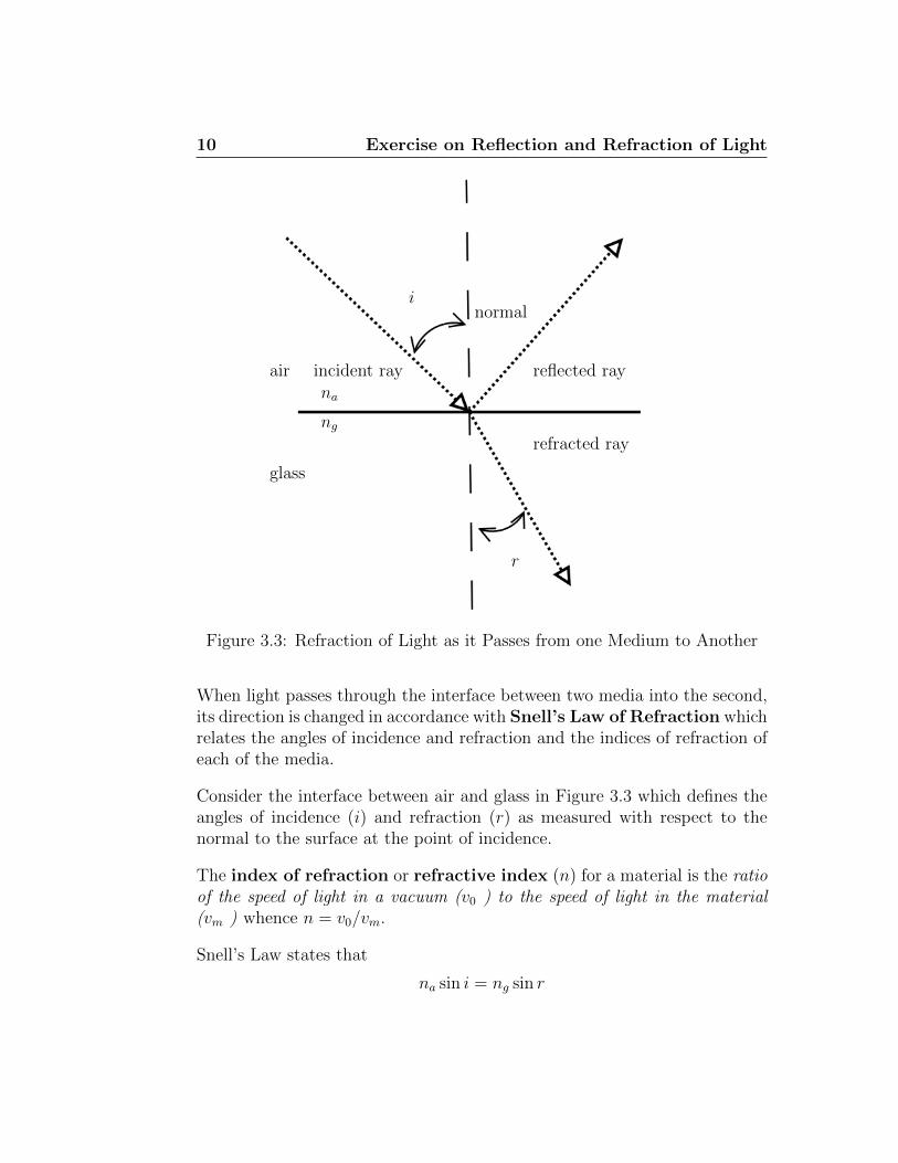
Figure 3.3: Refraction of Light as it Passes from one Medium to Another

When light passes through the interface between two media into the second,its direction is changed in accordance with Snell’s Law of Refraction whichrelates the angles of incidence and refraction and the indices of refraction ofeach of the media.

Consider the interface between air and glass in Figure 3.3 which defines theangles of incidence (i) and refraction (r) as measured with respect to thenormal to the surface at the point of incidence.

The index of refraction or refractive index (n) for a material is the ratioof the speed of light in a vacuum (v0 ) to the speed of light in the material(vm ) whence n = v0/vm.

Snell’s Law states that

na sin i = ng sin r

3.4 Procedure 11

where na is the refractive index of air, and to a very good approximation

na ≈ 1

We can thus rewrite Snell’s Law for air to glass as

sin i = ng sin r

where ng is the refractive index of the glass.

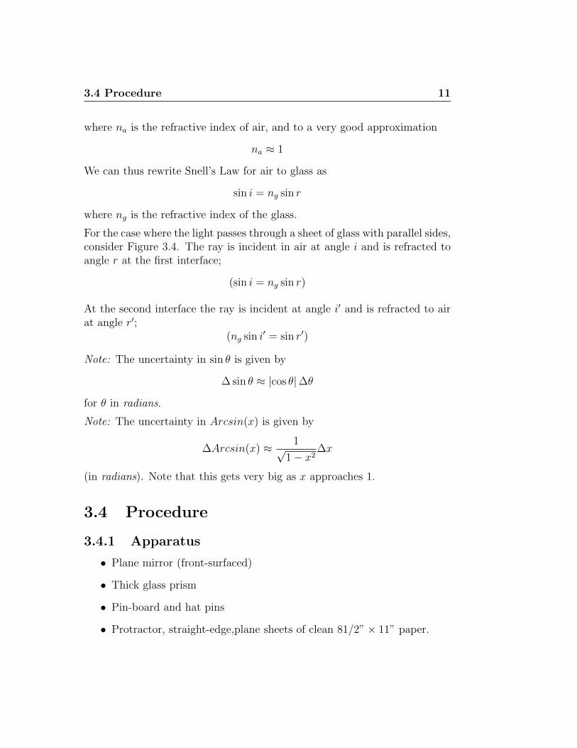
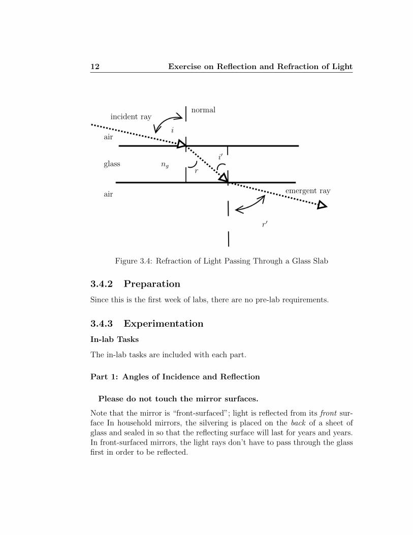
For the case where the light passes through a sheet of glass with parallel sides,consider Figure 3.4. The ray is incident in air at angle i and is refracted toangle r at the first interface;

(sin i = ng sin r)

At the second interface the ray is incident at angle i′ and is refracted to airat angle r′;

(ng sin i′ = sin r′)

Note: The uncertainty in sin θ is given by

∆ sin θ ≈ |cos θ|∆θ

for θ in radians.

Note: The uncertainty in Arcsin(x) is given by

∆Arcsin(x) ≈ 1√1− x2

∆x

(in radians). Note that this gets very big as x approaches 1.

3.4 Procedure

3.4.1 Apparatus

• Plane mirror (front-surfaced)

• Thick glass prism

• Pin-board and hat pins

• Protractor, straight-edge,plane sheets of clean 81/2”× 11” paper.


normalincident ray

emergent ray

air

glass

air

i

r

i′

r′

ng

Figure 3.4: Refraction of Light Passing Through a Glass Slab

3.4.2 Preparation

Since this is the first week of labs, there are no pre-lab requirements.

3.4.3 Experimentation

In-lab Tasks

The in-lab tasks are included with each part.

Part 1: Angles of Incidence and Reflection

Please do not touch the mirror surfaces.

Note that the mirror is “front-surfaced”; light is reflected from its front sur-face In household mirrors, the silvering is placed on the back of a sheet ofglass and sealed in so that the reflecting surface will last for years and years.In front-surfaced mirrors, the light rays don’t have to pass through the glassfirst in order to be reflected.

3.4 Procedure 13

1. Draw a line down the centre of a piece of clear paper and place it onthe pin-board. Set the mirror surface against this line near the centreof the page, standing on edge. On the front side of the mirror, off toone side, stick a hat-pin vertically into the pin-board to serve as anobject. Viewing the image of this pin in the mirror, place two hat pinsalong the direction of a reflected ray. Keep the two pins as far apart aspossible.

2. Remove the pins, and circle these three holes in the paper.

3. Repeat this procedure once more for another viewing direction, usingsomething other than circles to mark the other set of holes.

4. From each of the two sets of pin-holes you have the direction of thereflected ray, which you can extend to find the point of reflection at themirror. From the point of reflection and the object pin hole, you candraw the incident ray direction. Remove pins, mirror and sheet, anddraw in all incident and reflected rays and the surface normal at eachpoint of reflection. Measure the incident and reflected angles for eachof the rays and enter them in Table 3.1.

IT1: Show your diagram to the lab instructor.

Part 2: Virtual Images

1. Begin with paper, line, and mirror as in the previous part. Draw alarge letter V somewhere in front of the mirror. Mark the two ends ofthe V in some way (such as A, B, C) so that you can tell them apartin the reflection. Hint: Make the two arms of the V different lengthsand it will make them easier to distinguish.

2. Place a pin in one of the strategic points of the (object) letter, (sayA), and find the incident and reflected rays in two directions, labellingthem (such as A1 for the points in one direction, and and A2 for thetwo points in the other direction).

3. Repeat with hat-pins placed in the other strategic points of the objectletter.


4. Remove pins and mirror, and on the sheet extend each pair of reflectedrays back behind the mirror as dashed lines, to where they intersect.The three intersection points thus gained mark the strategic points ofthe virtual image of the letter used as an object. Draw in this virtualimage using dotted lines.

IT2: Show your diagram to the lab instructor.

Part 3: Refraction through Parallel Surfaces

1. Draw a line down the centre of a piece of paper as before. With paperon the pin board, place the glass prism standing on one of its longedges, against the line, centred on the page.

2. Draw a line along the back edge of the parallel-sided glass block on thepage.

3. Place a pin in the paper behind the prism off to one side. Observe froma position which will give a large angle of incidence. Use another pinon the same side of the paper so that you can map the incident ray.

4. With 2 more pins, map out the emergent ray. Remove the pins andlabel the 4 points.

5. Repeat the previous two steps for another object point.

6. Remove the prism.

7. Draw the incident and emergent rays for both cases, and then draw inthe rays refracted through the glass as well. Measure the angles i, r,i′ and r′ for both rays and record them in Table 3.2. Remember thatyou’ll have to draw in normal lines to measure the angles, or else use(90 − angle) if you measure from the glass surface. You may have toextend the rays inside the glass block in order to measure them.

Note that the emergent ray should be exactly parallel to the incidentray for each case.

IT3: Show your diagram and Table 3.2 to the lab instructor.

3.4 Procedure 15

Part 4: Refraction Through a Prism

1. Place the prism flat on one of its broad faces on a sheet of paper anddraw in its outline carefully.

2. Place 2 pins along a path to the prism with an incident angle i about45◦.

3. Look through the side of the prism where the refracted ray emerges,and place 2 pins along the line of the emergent ray.

4. Remove the prism. Draw lines connecting both sets of pins with thefaces of the prism, and then draw the line though the prism which joinsthem and thus trace the ray path through the prism experimentally.

5. Measure the incident, refracted, and emergent angles and put them inTable 3.4.

IT4: Show your diagram and Table 3.4 to the lab instructor.

3.4.4 Analysis

Post-lab Questions

Q1: Calculate ng and ∆ng from the data in Part 3, placing the results inTable 3.3.

1. Measure the prism angle from your diagram of Part 4, and use it alongwith the average n from Part 3 to calculate each of the angles in Ta-ble 3.5. Show your calculations.

2. Draw in the ray based on your calculations as it passes through theprism to the other face. Higlight this line to distinguish it from theexperimental one.

3. Draw in the ray as it leaves the second surface, based on your calcula-tions. Higlight this line to distinguish it from the experimental one.

4. Put all the calculations on the sheet with the prism outline and thecalculated ray path.


Post-lab Tasks

T1: Photocopy your diagram and your calculations and hand them in.

3.5 Bonus

Include uncertainties in the last part. Note that in each step, the uncertaintyin an angle makes an uncertainty in the position of the next refraction.

3.6 Recap

By the end of this exercise, you should know how to :

• Draw ray diagrams for

– reflection at a plane surface

– refraction at a plane interface

3.7 Summary

Item Number Received weight (%)Pre-lab Questions 0 0In-lab Questions 0 0Post-lab Questions 1 20

Pre-lab Tasks 0 0In-lab Tasks 4 60Post-lab Tasks 1 20

3.8 Template 17

3.8 Template

My name:My student number:My partner’s name:My other partner’s name:Today’s date:

ray Angle (degrees)i r

1

2

Table 3.1: Light reflecting from a mirror

ray Angle (degrees)i r i′ r′

1

2

Table 3.2: Light refracting through a slab


ray From incident From emergentn ∆n n ∆n

1

2

average(n)

uncertainty(∆n)

Table 3.3: Calculated index of refraction

ray Angle (degrees)i r i′ r′

1

Table 3.4: Light refracting through a prism

ray Angle (degrees)r ∆r i′ ∆i′ r′ ∆r′

1

Table 3.5: Calculated refraction angles

Chapter 4

Exercise on The BrewsterAngle

4.1 Purpose

The purpose of this lab is to investigate polarization by reflection and theBrewster angle.

4.2 Theory

The ‘vibrations’ of a light wave are transverse, i.e., light is an electromag-netic wave whose electric and magnetic field vectors are perpendicular to thedirection of propagation. This can be seen from the solutions to Maxwell’sequations for the electromagnetic field. The transverse nature of light wavesis illustrated diagrammatically Figure 4.1a , in which the radial arrows rep-resent vibrations taking place in all directions in a plane perpendicular tothe line of sight. For the purposes of analysis, it is convenient to describe thetransverse vibrations in terms of components resolved along two mutuallyperpendicular directions, XX and YY in Figure 4.1a .

In the case of ordinary, unpolarized light, energy is distributed uniformlyamong transverse vibrations in all possible directions, and the perpendicularcomponents are equal, regardless of the chosen directions of resolution.

In the case of completely polarized light, only one plane of vibration exists.This situation is illustrated in Figure 4.1b , where a polarizing device hasbeen used to select only the vertical components of all transverse vibrations

20 Exercise on The Brewster Angle

(a) (b) (c)

Figure 4.1: The Polarization of Light

in the incident light. It can be shown that the intensity of the polarized lightin Figure 4.1b is one-half of the original, unpolarized intensity.

Since the human eye is cannot distinguish between polarized and unpo-larized light, we require a polarizing device; an instrument that will transmitvibrations that take place only along one axis, known as the transmissionaxis. If the observed intensity remains the same for all orientations of theaxis, the light is unpolarized. If (virtually) no light is transmitted for aparticular orientation of the polarizer, the incident light is completely planepolarized, as shown in Figure 4.1c . Because the second polarizer in Fig-ure 4.1c is used to analyze the polarization of light incident upon it, it isreferred to as an analyzer. The plane of polarization of the light can thenreadily be determined by noting that the transmission axis of the analyzer isperpendicular to it when no light is transmitted.

4.2.1 Production of Polarized Light

Polarizing Screens

The simplest method of producing polarized light makes use of a polariz-ing screen, composed of either natural or artificially prepared crystals that

4.2 Theory 21

Figure 4.2: Brewster’s Law

possess the property of being able to transmit only the components of thetransverse vibrations parallel to a specific direction in the crystal. Tourma-line is an example of a natural crystal which does this, but it is obtainableonly small and imperfect specimens. A commercial product marketed underthe trade name of Polaroid R© is well suited to the construction of polarizingscreens of any size. It consists of a layer of iodo-quinine sulfate (herapathite)crystals suitably oriented and imbedded in a thin sheet of transparent cellu-loid. While the polarization produced by these screens is practically completethroughout most of the visible spectrum, the shortest violet and longest redends are only partially polarized. Since the eye (and most optical detec-tors designed to work in the visible) are not particularly sensitive to thesewavelengths, this limitation is not serious for most practical applications.

Polarization by Reflection

When a ray of light is incident on a smooth surface, the reflected componentis partially polarized, with the direction of maximum intensity parallel tothe surface (i.e., perpendicular to the plane of incidence). If the surface isthat of a transparent medium, the transmitted component is also partiallypolarized, but with the direction of maximum intensity parallel to the planeof incidence. This is illustrated in Figure 4.2 .


Of course, the reflected and transmitted rays are described by:

i = i′

andsin i = n sin r (4.1)

where i is the angle of incidence, i′ is the angle of reflection, r is the angle ofrefraction, and n is the index of refraction of the medium.

It was discovered by Malus in 1808 that, in the case of non-metallic sur-faces, when the angle of incidence is such that the angle between the reflectedand transmitted rays is 90◦, the reflected ray is completely polarized parallelto the surface. The particular angle of incidence for which this occurs iscalled the polarizing angle, and it depends on the index of refraction n.For glass, the polarizing angle is about 57◦.

The required angle of incidence can be derived from the geometry ofFigure 4.2 . According to Malus’ Law, complete polarization of the reflectedray occurs when i is such that the angle between the reflected ray and thetransmitted ray is 90◦. Then it follows from the geometry that

i+ r = 90◦

orr = 90◦ − i

Using this in Equation 4.1

sin i = n sin r = n sin (90◦ − i) = n cos i

orn = tan i

andi = arctann (4.2)

Equation 4.2 is known as Brewster’s Law, and the required angle of inci-dence is also known as the Brewster angle. At angles of incidence otherthan Brewster’s angle, the reflected light is partially polarized.

As mentioned previously, the transmitted component is also partially po-larized. By means of transmission through a number of parallel plates, therepeated reflection progressively increases the degree of polarization of the

4.2 Theory 23

Figure 4.3: Polarization by Successive Reflection

transmitted ray, until, (after 10 or twelve reflections), the transmitted rayis, for all practical purposes, completely polarized. From what has beensaid, it should be clear that the plane of polarization of the transmitted rayis perpendicular to that of the reflected ray. This process is illustrated inFigure 4.3 .

Thus, a stack of glass plates inclined at the Brewster angle with respectto the incident ray can be used as a polarizer in either of two ways, as shownin Figure 4.4 .

Polarizing screens are extensively used in photography for the eliminationof unwanted reflections and for lighting control. Anti–glare glasses are madewith Polaroid to reduce the glare produced by specular reflections from water,hard-surface roads, etc.

How would you orient the transmission axis of the glasses to accomplishthis?

Polarization by reflection can be used to construct analyzers to operatein spectral regions (such as the extreme ultraviolet) where the light wouldbe completely absorbed by any transmission through a medium. These areusually made of a series of front surface mirrors, (gold or aluminum plated),and produce polarizations of up to 99% , with about 10 to 20% of the incidentlight intensity emerging.


Figure 4.4: Polarization by Reflection and by Transmission

4.3 Procedure


Apparatus

The following equipment is required for this experiment:

• Polaroid R© filter

• spectrometer

• glass slides

• holder for slides

• light source

Method

Measuring the Brewster Angle

1. Place the holder with the glass plates on the prism table of the spec-trometer.

4.3 Procedure 25

2. Place a light source to send light through the collimator slit.

3. Hold a polarizing filter close to your eye and observe the reflected imageof the source, as shown in Figure 4.4a. Rotate the filter to find theminimum transimission (i.e. the dimmest image of the slit).

4. Rotate the prism table, and repeat the previous instruction until youfind the angle at which the slit becomes invisible as the filter is rotated.

5. Move the telescope into position so that the slit image is lined up withthe crosshairs.

6. Measure the angle of the telecope from the spectrometer scale andrecord it in Table 4.2.

7. Rotate the prism table 10 or twenty degrees, and then repeat the lastthree steps to determine the angle again. The difference between theseangles can be used to determine an uncertainty in the Brewster angle.

8. The Brewster angle should be 1/2 of the recorded angle.

9. Look at the other side of the glass plates to see the image transmittedthrough the plates.

10. Move the telescope into position so that the slit image is lined up withthe crosshairs, as before.

11. Measure the angle of the telecope from the spectrometer scale andrecord it.

Inlab Questions

IQ1: Why should the Brewster angle be half of the measured angle?

IQ2: Is the transmitted image of the slit at 90◦ to the reflected image?Explain. (Hint: Look carefully at Figures 4.2 and 4.3.)

IQ3: If you turned the plates so that the reflected image was on the otherside of where it is now, how would your calculation of the Brewster anglechange?

IQ4: Write out one sample conversion from degrees, minutes, and seconds(DMS) to decimal degrees (DD).

IQ5: Write out your calculation of the Brewster angle and its uncertainty.


Inlab Tasks

IT1: Sketch the experimental layout in your lab book.

IT2: Sketch the spectrometer scale for one measurement in Table 4.1 andshow the corresponding measurement to show that you can use the Vernierscale correctly. (Be sure to show both the main and Vernier scales.)

IT3: Demonstrate the Brewster angle and summarize your findings to thelab instructor.

4.3.2 Analysis

Postlab Questions

Q1: Calculate the index of refraction of the glass from Brewster’s Law. Showyour calculations.

Postlab Tasks

T1: Hand in the question answers, along with a copy of your sketch of thesetup.

4.4 Recap

By the end of this exercise, you should know how to :

• find and measure the Brewster angle, and

• use it to calculate the index of refraction

To do this, you will have to learn how to read the spectrometer.

4.5 Summary 27

4.5 Summary




4.6 Template


Table 4.1: Sketch of spectrometer scales

Trial Angle (degrees)1

2

Table 4.2: Angle where maximum polarization is observed

Chapter 5

Exercise on the MichelsonInterferometer

5.1 Purpose

The purpose of this lab is to use the Micheleson interferometer to detectsmall differences in index of refraction.

5.2 Theory

In the Michelson interferometer, a beam of light is split in two and laterrecombined. An interference pattern is produced when the two beams re-combine. The pattern will be affected if there is a difference in the opticalpath length of the two arms of the interferometer. If an air cell is placedin one of the arms, then the path length in that arm will be different thanif there were a vacuum in place of the air cell, since the index of refractionfor air is not the same as for a vacuum. If we observe the interference pat-tern while air is removed from the air cell, then the change can be used todetermine the difference between the indices of refraction of air and vacuum.

Due to the air being withdrawn, the total change in optical path length is

∆L = 2(n− 1)t (5.1)

where n is the index of refraction of air at the wavelength used, and t is thethickness of the air cell. This change in optical path length may also be given

30 Exercise on the Michelson Interferometer

by

∆L = λ∆m (5.2)

since when the total optical path difference is an odd multiple of λ/2, con-structive interference occurs and when the optical path difference is an evenmultiple of λ/2, destructive interference occurs.

Thus, when t, ∆m, and λ are known, n− 1 is easily calculated.

5.3 Procedure

5.3.1 Apparatus


• vacuum pump, Michelson Interferometer with air cell

• Na lamp, Hg lamp, laser with beam spreader

5.3.2 Preparation

Pre-lab Tasks

PT1: Read the section on the Michelson interferometer on pages 408 and409 of your text.

Pre-Lab Questions

PQ1: Combine and rearrange Equations 5.1 and 5.2 to determine how alinear graph of ∆m vs. 1

λmay be produced, and show how n − 1 may be

derived from the graph.


1. Using green light from the Hg lamp (λ = 5461A), produce circularinterference fringes by adjusting the planes of the fixed mirrors. Theair cell should be in place in one of the arms. Use a vacuum pump towithdraw the air from the cell.

5.3 Procedure 31

2. Count the number of fringes, ∆m that appear or disappear. It may beeasier to determine ∆m while air is admitted into the cell.

3. Repeat this several times and average the results for consistency.

4. Repeat the above procedure using the Na lamp, and any other sourcepossible. Some possibilities are the Mercury light (with the approriatefilter) for the yellow lines at 5770 Aand 5790 A, the Mercury light (withthe approriate filter) for the blue line at 4358 A.

5. Measure the inside thickness of the air cell.

Inlab Questions

IQ1: Did the number of fringes change monotonically with the wavelengthof light? Did it change in the direction expected?

Inlab Tasks

IT1: Summarize your results to the lab instructor.

5.3.4 Analysis

1. Plot the linearized graph, and do a least squares fit.

Postlab Discussion Questions

Q1: Calculate the index of refraction of air from the results of the leastsquares fit, and compare this with the expected value. Does the y-interceptof your graph match your expectations? Explain.

Postlab Tasks

T1: Hand in the question answers, along with the graph and your calcula-tions.


5.4 Recap

By the end of this exercise, you should know how to use a Michelson inter-ferometer.

5.5 Summary



5.6 Template 33

5.6 Template


wavelength number of fringes(A)

Table 5.1: Mercury lamp data


Chapter 6

Exercise on Newton’s Rings

6.1 Purpose

The purpose of this lab is to investigate interference in thin films.

6.2 Theory

Various methods of producing interference fringes can be classified into twotypes:

1. division of a wavefront into two or more beams (double slit, Lloydmirror, Fresnel biprism) which are later recombined, and

2. division of the amplitude of an extended portion of the wavefront intobeams which are later recombined

Unlike the division of the wavefront, thin film interference does not requirea narrow line source or meticulous alignment of auxiliary equipment. Thefamiliar colours in soap films and oil slicks are excellent examples of thin filminterference.

When light is incident on a thin film, part of it is reflected from the firstsurface, and part is reflected from the second surface. These recombine atthe first surface to form the reflected beam, and the rest combine to formthe transmitted beam at the second surface. Because of the optical path dif-ference between the two reflected beams, a phase difference exists between

36 Exercise on Newton’s Rings

these beams, leading to interference effects. In addition, there are phase dif-ferences introduced because of reflections. Whenever reflection occurs froman optically denser medium, a phase change of π is introduced. Thus, whenthe total optical path difference is an odd multiple of λ/2, constructive in-terference occurs. When the optical path difference is an even multiple ofλ/2, destructive interference occurs. These effects result in the formation ofinterference fringes as observed with the reflected light. Fringes also occur inthe transmitted beam, except that these are the complement of the reflectedfringes, and are much harder to observe.

The fringes are essentially constant thickness contours of the film. Theycan be used to map the irregularities in the film thickness and/or deter-mine the film thickness. The Michelson Interferometer and the Fabry-PerotInterferometer are good examples of devices operating on this principle.

6.2.1 Newton’s Rings

Newton’s Rings form a circular interference pattern due to the reflectionsoccurring in an air wedge, formed around the point of contact between aspherical surface and a plane surface, as shown in Figure 6.1.

Let rm be the radius of the mth dark ring. A is the center of curvature,B is the point of contact, and R is the radius of the spherical surface ofthe plano-convex lens. Note that m is an integer, and h is the height of thesurface of the lens above the plane surface at radius rm.

From the geometry, it can be shown that

r2m = 2Rh− h2 (6.1)

for this setup.

Then mλ = 2h, and a dark fringe is produced at the center (because ofthe phase change due to reflection). Since h� R, this means

r2m ≈ 2Rh = Rmλ

If rm is measured as a function of m for different values of λ, and a graph ofr2m vs mλ is plotted, a straight line with slope R should be obtained.

6.2 Theory 37

B

A

R R

h

rmXXXy ��:

Figure 6.1: Plano–Convex Lens


Observer

Travelling Microscope

Thin Glass Plate Parallel Light

Plano-Convex Lens

Optical Flat

Figure 6.2: Newton’s Rings Setup

6.3 Procedure 39

6.3 Procedure

6.3.1 Preparation

Pre-lab Tasks

PT1: Read the section on the Newton’s rings on pages 406 and 407 of yourtext.

Pre-Lab Questions

PQ1: Derive Equation 6.1.

6.3.2 Apparatus


• planoconvex lens, glass plates, lens holders

• Na lamp


Measurement of Fringe Diameters

Figure 6.2 shows the experimental arrangement to be used. Light from theNa arc lamp (λ = 5893A) is reflected to the flat surface of the plano-convexlens by a thin glass plate inclined at 45◦ to the vertical. Light is reflected atthe boundaries of the air film between the lens and the optical flat. These tworeflections pass through the glass plate into the travelling telescope, whichmagnifies the rings and can be used to measure their diameters.

1. Carefully adjust the telescope so that the center of the cross-hairs passthrough the center of the fringe pattern (travelling at right angles tothe fringes).

2. Set the cross-hairs tangentially on each dark ring, beginning at the10th ring on one side, and moving over to the 10th ring on the otherside. Record the positions of each dark ring as a function of m. Thediameters of each ring can be found from these measurements.


3. If the order of the central dark spot is m = 0, make a table of r2m vs m.

4. After measuring the fringes, replace the lens with a reticule and mea-sure a wide spacing on it so that you can determine the calibration forthe microscope.

Inlab Questions

IQ1: Using the calibration of the reticule, determine the diameter of thebiggest ring which you measured. Does the value fit with what you canobserve by eye?

Inlab Tasks

IT1: Summarize your results to the lab instructor.

6.3.4 Analysis

1. Determine the slope and y-intercept of the line passing through yourdata points.

Postlab Discussion Questions

Q1: Calculate the value of R. Does it seem reasonable?

Q2:Does the y-intercept of your graph make sense? Explain.

Postlab Tasks

T1: Hand in the question answers, along with the graph and your calcula-tions.

6.4 Recap

By the end of this exercise, you should know how to use and calibrate amicrometer scale.

6.5 Summary 41

6.5 Summary




6.6 Template


fringe number reading(left)

reading(right)

1

2

3

4

5

6

7

8

9

10

Table 6.1: ?

Chapter 7

Exercise on Generalized LeastSquares Fitting

7.1 Purpose

The purpose of this exercise is to show you how to do least sqaures fits topolynomial functions in Excel TM.

7.2 Introduction

Previously you have done curve fitting in two dimensions. Now you will learnhow to extend that to multiple dimensions.

7.3 Theory

7.3.1 Non-linear

Linearizable

Some equations, such asy = Ae(Bx)

can be treated fairly simply. Linearize and do a linear least squares fit, asyou have done in the past. (Note: “Least Squares” applies to transformedquantities, not original ones so gives a different answer than you would getfrom a least squares fit in the untransformed quantities; remember in general

44 Exercise on Generalized Least Squares Fitting

the idea of a line of “best fit” is not unique. For example, for the equationshown, ln y vs. x is linear, so you can do a least squares fit in ln y, but thiswill not give the same result as a least squares fit in y, since the sum ofsquares of ln y will depend on the data in a different way than the sum ofsquares in y.)

7.3.2 Linear

General

Some equations, such as this

y = b0 + b1x1 + b2x2 + · · · bkxk

are linear, although in multiple variables. We can create a matrix of inde-pendent data

X =

x11 x12 . . . x1kx21 x22 . . . x2k...

.... . .

...xn1 xn2 . . . xnk

from the x values, where xij means variable xj for data point i and form avector of dependent data

Y =

y1...yn

where yi is the y data for data point i.

This creates a system which can be solved using functions in a spread-sheet.

Polynomial

Consider an equation such as this:

y = b0 + b1x+ b2x2 + · · · bkxk

This is just a special case of the previous situation above, eg. x1 = x, x2 = x2,x3 = x3, etc. (or x1 = 1/x, x2 = 1/x2 , etc.)

7.3 Theory 45

What about fit with skipped orders?eg. y = a+ b/x2 + c/x5

In this case, x1 = 1/x2, x2 = 1/x5.

A linear or polynomial least squares fit does not need starting values forparameters like the solver function would need.

7.3.3 Goodness of fit

Often you must choose between different fits because you do not know whattype of equation to use. In this case you want to be able to answer thequestion “Which fit is better?”

1. If both fits have the same number of parameters, then the better fit isthe one with the smaller SSE in the same quantity. (In other words,if you’re comparing a fit in y vs. x to one in ln y vs. x, you will firsthave to calculate the SSE of both in y vs. x. If you have linearizedan equation to calculate a fit, you can still use that fit to calculate theSSE in the original quantity afterward.)

2. One or both of the fits may have some parameters which are not “sta-tistically significant”; (i.e. lots of parameters close to 0 are probablymeaningless.) How close to 0 is “close enough”?

• RULE: Adding more parameters→ smaller SSE, (however a smallchange in SSE may not be significant.) Whether or not the addedparameters are significant can be determined statistically if the fitis a linear one or one which can be linearized.

To actually determine whether the change is big enough, proceed asfollows:

(a) Do fit with g + 1 parameters (as above); calculate the sum ofsquares error and call it SSE1. If you use regression from aspreadsheet, you can determine SSE from the results. RememberSSE1 = s1

2ν1; in this case ν1 = n− (g + 1).

(b) Do fit with k+1 parameters (as above); calculate SSE2. As above,SSE2 = s2

2ν2 and in this case ν2 = n− (k + 1).


(c) Calculate s3 as follows:

s3 =

√SSE1 − SSE2

k − g

and let ν3 = k − g.

(d) Calculate F as follows:

F =s3

2

s22

If F is big, then include the extra parameters. (In this case, itmeans the SSE changed a lot by adding the extra parameters,which is what would happen if they were really important.) Howbig is “big”?

(e) Look up Fα,ν3,ν2 from a table of the F distribution in a statis-tics text1, where α determines the confidence interval; typicallyα = 0.05 for a 95% confidence interval. If the F you calculatedis greater than the table value, then keep the extra parameters.Note: In the table, you are given quantities ν1 and ν2; you shoulduse your calculated value of ν3 in place of ν1 in the table. Doingit this way keeps the table in the same form you will find it in astatistics text.

The following example illustrates how to do this for a linear fit. Usually wewant to compare two fits; in this example, we will compare 3 fits to illustratethe process more clearly. We will compare 2 fits at a time, and in each casewe will use g + 1 to denote the number of parameters in the “smaller” fit 2

, and k + 1 to denote the number of parameters in the “bigger” fit, so k isalways bigger than g.

7.4 Example

Consider the data shown in Table 7.1 and plotted in Figure 7.1. (Error barshave been omitted for simplicity.)

1You can also use the FINV function of a spreadsheet like Excel or OpenOffice.2Why not just g? Because g is the degree of the polynomial, which has g+1 parameters.

For example a polynomial of degree 2, such as Ax2 + Bx + C has 3 parameters, namelyA, B, and C.

7.4 Example 47

x y

100 185 270 450 836 1520 2510 45

Table 7.1: Sample Data

Figure 7.1: Plot of Sample Data

It should be obvious that some possible equations for a fit to this datamay be polynomials in 1/x.

A fit to y = A+B/x gives us Table 7.2.

Notice that the curve cannot “bend enough”, and so we will see whathappens if we add another parameter. To do this we simply add anothercolumn to the data, and change LINEST so that it now points to the newblock of x data, which includes two columns.


1/x y

0.0100 10.0118 20.0143 40.0200 80.0278 150.0500 250.1000 45

Table 7.2: Data for Fit to A+B/x

B 488.15 -2.02 AσB 30.56 1.37 σAR2 0.98 2.43 s

255.18 5 ν1502 29.43 SSE

Table 7.3: LINEST 2 parameter output

Figure 7.2: Graph of Fit to A+B/x

7.4 Example 49

1/x 1/x2 y

0.01000 0.000100 10.01176 0.000138 20.01429 0.000204 40.02000 0.000400 80.02778 0.000772 150.05000 0.002500 250.10000 0.010000 45

Table 7.4: Data for Fit to A+B/x+ C/x2

C -2713.14 784.5 -6.45 AσC 562.24 62.79 1.09 σAR2 1 1.04 #N/A

707.95 4 #N/A1527.11 4.31 #N/A


Note how the parameters are rearranged when there are more of them.(The parameters are actually arranged on the top row of the output in reverseorder of the data columns.)

It’s now possible to compare the two fits to see if the third parametermakes a big enough change to keep. To do that, we do the following:

1. Get s for the fit with more parameters. (We’ll refer to this as the “big”fit.) Call this s2. In our example, that would be s2 = 1.04.

2. Calculate s3 due to the difference of the fits. Since we’re only checkingfor the effect of one parameter,

s3 =

√SSEsmall − SSEbig

νsmall − νbig=

√29.43− 4.31

1=√

25.12 = 5.01

3. Calculate F = s32

s22= 5.012

1.042= 23.2


4. Look up the value of F0.05,νsmall−νbig ,νbig = F0.05,1,4 or calculate it usingthe FINV function of a spreadsheet. (The values go in the order given.)From Table 7.9, F0.05,1,4 = 7.71 is the value to compare.

5. Since our calculated value for F is bigger than the value from the table,that means our extra parameter made a big difference, so we shouldkeep it.

7.4 Example 51

Figure 7.3: Graph of Fit to A+B/x+ C/x2

This process can be repeated as many times as we wish.


1/x 1/x2 1/x3 y

0.01000 0.000100 0.00000100 10.01176 0.000138 0.00000163 20.01429 0.000204 0.00000292 40.02000 0.000400 0.00000800 80.02778 0.000772 0.00002143 150.05000 0.002500 0.00012500 250.10000 0.010000 0.00100000 45

Table 7.6: Data for Fit to A+B/x+ C/x2 +D/x3

D 60476.14 -12121.37 1156.6 -9.93 AσD 29909.81 4672.18 189.98 1.91 σAR2 1 0.78 #N/A #N/A

837.72 3 #N/A #N/A1529.6 1.83 #N/A #N/A


It is not immediately obvious which of the above curves fits the data“best”. We could even go on adding higher and higher powers of 1/x untilwe had no more degrees of freedom 3 left, but once we get no significantchange, it’s time to stop.

Table 7.8 summarizes the results of the various fits.

3The number of degrees of freedom in a fit is the number of data points beyond thebare minimum for that fit. So, for an average it is n − 1, since only one value is needed;for a straight line it is n− 2, since two points are needed, etc. In general,

ν = n−m

where m is the number of parameters in the fit to be determined. Note that when youhave no degrees of freedom, you have no idea of the “goodness” of your data, and thuscannot determine the standard deviation. Once you have even one degree of freedom, youcan do so.

7.4 Example 53

Quantity FitA+B/x A+B/x+ C/x2 A+B/x+ C/x2 +D/x3

s 2.43 1.04 0.78ν 5 4 3

SSE 29.43 4.31 1.83A -2.02 -6.45 -9.93σA 1.37 1.09 1.91B 488.15 784.5 1156.6σB 30.56 62.79 189.98C -2713.14 -12121.37σC 562.24 4672.18D 60476.14σD 29909.81

Table 7.8: Comparisson of Fit Parameters

• Note that the SSE gets smaller as the number of parameters increases,but the change gets smaller.

• Note also that when a parameter is added, all of the previous parame-ters change as well.

• Even though it is considered “insignificant”, the D parameter is biggerthan all of the rest! (However, note the size of its standard error.Remember also that it gets divided by x3, which will range in size from1000→ 1000000.)


Figure 7.4: Graph of Fit to A+B/x+ C/x2 +D/x3

7.5 Procedure

7.5.1 Investigation

The following functions are polynomials in 1λ

or something similar. Set upthe appropriate tables for each and use LINEST to do a least squares fit foreach.

Then use the goodness of fit criteria to determine the best.

n = A+B

λ(7.1)

n = A+B

λ2(7.2)

n = A+B

λ+C

λ2(7.3)

n = A+B

λ2+C

λ4(7.4)

7.5 Procedure 55

ν2 \ ν1 1 2 3 4 5 6 · · · ∞1 161.4 199.5 215.7 224.6 230.2 234 · · · 254.32 18.51 19 19.16 19.25 19.3 19.33 · · · 19.53 10.13 9.55 9.28 9.12 9.01 8.94 · · · 8.534 7.71 6.94 6.59 6.39 6.26 6.16 · · · 5.635 6.61 5.79 5.41 5.19 5.05 4.95 · · · 4.366 5.99 5.14 4.76 4.53 4.39 4.28 · · · 3.67...

......

......

......

. . ....

∞ 3.84 3 2.6 2.37 2.21 2.1 · · · 1

Table 7.9: F–Distribution Table (α = 0.05)

Using LINEST for the first two parameter fit

• Put the function in C20, with constant=1 and stats=1.

• Highlight C20 to D24.

• Press 〈F2〉 followed by 〈CTRL〉〈SHIFT〉〈ENTER〉.

• Some of the important parameter names have been indicated.

For the second two parameter fit, you can just copy and paste as needed(or adapt the steps above for the new location.)

Using LINEST for the three parameter fits

It works in a similar way, but instead of C20 to D24, highlight C20 to E24.(There is one more parameter so another column is needed.) Note the waythe parameters are arranged in this case.

Inlab Tasks

IT1: Do each of the fits above and fill in Table 7.10.

IT2: Use the F test to determine whether fit 7.3 is better than fit 7.1 orfit 7.2.


Inlab Questions

IQ1: Based on the SSE values, which was better; fit 7.1 or fit 7.2?

IQ2: Based on the SSE values, which was better; fit 7.3 or fit 7.4?

7.6 Summary



7.7 Template 57

7.7 Template


Fit A σA B σB C σC SSE

7.17.27.37.4

Table 7.10: Fit comparison


Chapter 8

Thin Lenses

8.1 Purpose

In this experiment we measure the focal lengths of two thin converging lenses,observe real and virtual images in lenses, build a simple telescope, and makeuse of the simple lens formula.

8.2 Introduction

8.3 Theory

Lenses work by virtue of the refraction of light at their spherically shaped sur-faces. Any spherically shaped interface between media with different indicesof refraction, both of which are transparent, will have focusing or defocusingeffects on light passing through it.

A simple thin lens has two spherical surfaces, one on each side of a pieceof glass. The centres of curvature of the lens surfaces define a straight linecalled the optic axis of the lens, as shown in Figure 8.1. (A and B are thecentres of curvature of the two spherical lens surfaces.)

The focal point of a lens, or back focus F ′ is defined as that point on theoptic axis at which parallel rays incident on the lens are brought to a focusbehind the lens. See Figure 8.2.

Figure 8.2 also defines-f , the focal length of the lens as the distancefrom the lens centre to the back focal point.

60 Thin Lenses

optic axis

lens

r1

r2

A B

Figure 8.1: Light Passing Through a Thin Lens

optic axis

f -�

F ′

Figure 8.2: Location of Back Focus

8.3 Theory 61

focal plane

Figure 8.3: Focal Plane of a Lens

An imaginary plane perpendicular to the optic axis through the backfocus is called the focal plane of the lens. This focal plane has the propertythat all sets of parallel rays incident on the lens are focused on it, as inFigure 8.3.

The properties of a thin lens are symmetric about its central plane allow-ing us to define a second focal point called the front focal point F , alsoat distance f from the lens centre. Rays emanating from this front focalpoint toward the lens emerge from the lens parallel to the optic axis as inFigure 8.4.

Figure 8.5 shows a thin converging lens with an object (an arrow) locateda distance S from the lens centre. S is the object distance. The locationof the real image of the object is determined graphically by drawing threeprincipal rays from the tip of the object arrow:

1. parallel to the optic axis before reaching the lens, then through F ′

2. straight through the lens centre (undeviated by the lens)

3. through F to lens, emerging parallel to the optic axis

The point where these principal rays intersect is the image of the tip ofthe object arrow. The image is located at image distance S ′ from the lenscentre. Note that the image thus formed is a real image because rays fromthe object actually form the image. This means the image can be displayedon a screen.

62 Thin Lenses

F

f -�

Figure 8.4: Front Focal Point

opticaxis

object

image

S ′ -�

F ′

S -�

F

Figure 8.5: Important Points in the Object and Image Planes

8.4 Procedure 63

This geometrical construction with the principal rays can be replacedwith algebra; the lens formula is

1

S+

1

S ′=

1

f

with all quantities as defined in the diagram.

8.4 Procedure

8.4.1 Apparatus

• A “meter-stick” optical bench on stands

• Two lenses of different focal length

• Lighted object & screen

• Holders for lenses, screens, and a mirror

8.4.2 Preparation

Pre-lab Questions

PQ1:

Pre-lab Tasks

PT1:


Inlab Questions

IQ1:

In-lab Tasks

IT1:

64 Thin Lenses

Part 1: Focal Length of Converging Lenses

Please don’t get the lens surfaces dirty, and set them down only in theirholders or on a sheet of paper.

1. Place one of the lenses in its holder, and mount it and the screen onthe optical bench. Find the image of a distant object on the screen(the lights on the ceiling, for example) and measure the lens–to–imagedistance carefully. This will give a quite good measurement of f . Re-peat using the other lens. Note, f measured this way is accurate onlyif the object is far enough away that light from it can be considered tobe parallel.

Part 2: Autocollimation Method for Focal Length

1. Another bench method can be used to measure f , called autocollima-tion. Mount the illuminated object at one end of the optical bench.Mount one of the lenses in its holder on the bench, and also the flat mir-ror in the screen holder. These pieces should be in order; object, lens,mirror. Slide the lens and mirror together until their mounts touch onthe bench, then, slide mirror and lens together until a clear image ofthe object can be seen on the card holding the object. Slightly turningthe mirror will facilitate this, such that the image is on the object cardbeside the object. In this case the focal length is the distance from thelens centre to the object-image card. Measure this distance with care,and find the focal length with this method for the other lens as well.

2. Draw a ray diagram in your lab book (practise on a rough-work sheetfirst!) to illustrate the distant-object method of determining f .

3. Draw a ray diagram in your lab book to illustrate the autocollimationmethod of finding f (Hint: recall how the focal plane was defined andassume the object and its image coincide at the focal plane of the lens.

Part 3: Lens Formula Method for Focal Length

8.4 Procedure 65

Yet another method of determining f is through use of the lens formula.

1. Set up the illuminated object at one end of the bench, and mount onelens and the screen on the bench. For 5 well–separated object distances,(each larger than f), measure the object distance and determine theimage distance for each case. Repeat for the other lens.

2. For each lens, plot 1/S ′ against 1/S and draw a straight line through thepoints thus determining the intercepts on both axes. Either intercept(by the lens formula) is equal to the reciprocal of the focal length.

Part 4: The Refracting Telescope

1. Set up the small lens in its holder on the optical bench near one end.Place the large lens in its holder on-the bench a distance from the smallone equal to the sum of the focal lengths of both lenses. Use this as atelescope using the small lens as the eyepiece to view distant objects.Draw a ray diagram for the refracting telescope assuming the objectdistance is very large (i.e. off the page).

Would the telescope produce an image of a distant object on a screenheld where the eye was in using the telescope?

Part 5: Simple Magnifier

1. Using the small lens, view any object with the object distance less thanthe focal length of the lens. Draw a ray diagram for this case in yourlab book.

Is the image

• real or virtual?

• erect or inverted?

• magnified?

This device is called a simple magnifier.

66 Thin Lenses

8.4.4 Analysis

Post-lab Questions

Q1: Calculate ng and δng.

Post-lab Tasks

T1:

8.5 Bonus

8.6 Summary



Appendix A

Aligning the Spectrometer

A.1 Introduction

To align the spectrometer you will need the following pieces of equipment:

• Spectrometer,

• Bubble Level,

• 60◦ Prism,

• Front Surface Mirror,

• small Allen wrench, screwdriver,

• Variable Intensity White–Light Source.

A.1.1 Levelling the Spectrometer

1. Place the spectrometer on the laboratory table so that it will be con-venient to rotate the telescope when making observations.

2. Place the bubble level on the base of the spectrometer and use shims(at 3 points separated by 120◦) to level it.

3. Adjust the height of the prism table so that the prism face is centeredon the telescope and collimator lenses.

68 Aligning the Spectrometer

Figure A.1: Telescope Adjustment

4. Place the bubble level on the prism table and rotate the table so thatthe adjusting screws are opposite the corresponding shims on the spec-trometer base. Level the prism table using the adjusting screws.

5. Rotate the prism table through 60◦ and adjust the shims on the tableso that the prism table is once again level.

6. Rotate the prism table in the same direction through another 60◦ andadjust the screws so that the table is level.

7. Repeat the previous two steps until the prism table is level in all posi-tions.

A.1.2 Telescope Adjustment

1. Figure A.1 shows a schematic view of the telescope used in this partof the experiment. Do not poke anything down the cross–hair tube,since the cross–hairs may be damaged or moved out of their pre-alignedposition.

2. Make sure that the opening in the eyepiece coincides with the openingin the cross–hair tube. Adjust the eyepiece until the cross–hairs are insharp focus.

A.1 Introduction 69

Figure A.2: Collimator Adjustment

3. Place the front surface mirror across the objective lens and shine light(from the white–light source) into the opening. Look into the eyepieceand observe the cross–hairs and their reflected image. Loosen the fo-cusing screw and adjust the cross–hair tube until the reflected image ofthe cross–hairs is in sharp focus and there is no parallax with respect tothe real cross-hairs. Lock the tube into this position with the focusingscrew.

4. Remove the front surface mirror and place the prism on its table withthe polished face perpendicular to the table surface. Shine white lightinto the opening and rotate the table until the cross–hairs and theirreflected image can be seen through the eyepiece. Adjust the levelingscrew on the telescope until the cross–hairs coincide with their image.The telescope has now been aligned to accept parallel light rays.

A.1.3 Collimator Alignment

1. Figure A.2 shows a schematic view of the collimator. Remove the prismfrom the table. Open the adjustable slit of the collimator and placethe white–light source in front of it.

2. Rotate the telescope until its cross–hairs are aligned with the adjustableslit. Adjust the leveling screw of the collimator until the slit is in thecenter of the eyepiece’s field of view.

70 Aligning the Spectrometer

3. Loosen the focusing screw of the collimator, and adjust the collimatortube until the slit is in sharp focus. Now reduce the slit width (do notclose the slit completely!) until the slit image is slightly larger thanthe cross–hairs, and remove any parallax between the slit image andcross–hairs. Lock the collimator into this position with the focusingscrew. The collimator has now been aligned to produce parallel lightrays.

Documents

PC237 Lab Manual - Wilfrid Laurier University