PC131 Lab Manual

c©Terry Sturtevant1 2

September 5, 2006

1Physics Lab Supervisor2This document may be freely copied as long as this page is included.

ii

Contents

1 Lab Manual Layout 1

1.1 This is a Reference . . . . . . . . . . . . . . . . . . . . . . . . 1

1.2 Parts of the Manual . . . . . . . . . . . . . . . . . . . . . . . . 1

1.3 Lab Exercises and Experiment Descriptions . . . . . . . . . . 1

1.4 Templates . . . . . . . . . . . . . . . . . . . . . . . . . . . . . 5

1.4.1 Table format in templates and lab reports . . . . . . . 5

1.4.2 Template tables . . . . . . . . . . . . . . . . . . . . . . 5

1.4.3 Before the lab . . . . . . . . . . . . . . . . . . . . . . . 6

1.4.4 In the lab . . . . . . . . . . . . . . . . . . . . . . . . . 7

1.4.5 Spreadsheet Templates . . . . . . . . . . . . . . . . . . 9

2 Goals for PC131 Labs 11

3 Instructions for PC131 Labs 13

3.1 Expectations . . . . . . . . . . . . . . . . . . . . . . . . . . . 14

3.2 Workload . . . . . . . . . . . . . . . . . . . . . . . . . . . . . 15

3.3 Administration . . . . . . . . . . . . . . . . . . . . . . . . . . 16

3.4 Plagiarism . . . . . . . . . . . . . . . . . . . . . . . . . . . . . 17

3.5 Calculation of marks . . . . . . . . . . . . . . . . . . . . . . . 17

4 How To Prepare for a Lab 19

5 Plagiarism 21

5.1 Plagiarism vs. Copyright Violation . . . . . . . . . . . . . . . 21

5.2 Plagiarism Within the University . . . . . . . . . . . . . . . . 21

5.3 How to Avoid Plagiarism . . . . . . . . . . . . . . . . . . . . . 23

iv CONTENTS

6 Lab Reports 256.1 Format of a Lab Report . . . . . . . . . . . . . . . . . . . . . 25

6.1.1 Title . . . . . . . . . . . . . . . . . . . . . . . . . . . . 256.1.2 Purpose . . . . . . . . . . . . . . . . . . . . . . . . . . 266.1.3 Introduction . . . . . . . . . . . . . . . . . . . . . . . . 266.1.4 Procedure . . . . . . . . . . . . . . . . . . . . . . . . . 276.1.5 Experimental Results . . . . . . . . . . . . . . . . . . . 276.1.6 Discussion . . . . . . . . . . . . . . . . . . . . . . . . . 296.1.7 Conclusions . . . . . . . . . . . . . . . . . . . . . . . . 306.1.8 References . . . . . . . . . . . . . . . . . . . . . . . . . 31

6.2 Final Remarks . . . . . . . . . . . . . . . . . . . . . . . . . . . 316.3 Note on Lab Exercises . . . . . . . . . . . . . . . . . . . . . . 31

7 Measurement and Uncertainties 337.1 Errors and Uncertainties . . . . . . . . . . . . . . . . . . . . . 337.2 Single Measurement Uncertainties . . . . . . . . . . . . . . . . 34

7.2.1 Expressing Quantities with Uncertainties . . . . . . . . 347.2.2 Random and Systematic Errors . . . . . . . . . . . . . 347.2.3 Recording Precision with a Measurement . . . . . . . . 357.2.4 Realistic Uncertainties . . . . . . . . . . . . . . . . . . 367.2.5 Zero Error . . . . . . . . . . . . . . . . . . . . . . . . . 38

7.3 Precision and Accuracy . . . . . . . . . . . . . . . . . . . . . . 387.3.1 Precision . . . . . . . . . . . . . . . . . . . . . . . . . . 387.3.2 Accuracy . . . . . . . . . . . . . . . . . . . . . . . . . 39

7.4 Significant Figures . . . . . . . . . . . . . . . . . . . . . . . . 407.4.1 Significant Figures in Numbers with Uncertainties . . . 417.4.2 Rounding Off Numbers . . . . . . . . . . . . . . . . . . 41

7.5 How to Write Uncertainties . . . . . . . . . . . . . . . . . . . 427.5.1 Absolute Uncertainty . . . . . . . . . . . . . . . . . . . 427.5.2 Percentage Uncertainty . . . . . . . . . . . . . . . . . . 427.5.3 Relative Uncertainty . . . . . . . . . . . . . . . . . . . 43

7.6 Bounds on Uncertainty . . . . . . . . . . . . . . . . . . . . . . 43

8 Repeated Independent Measurement Uncertainties 458.1 Arithmetic Mean (Average) . . . . . . . . . . . . . . . . . . . 468.2 Deviation . . . . . . . . . . . . . . . . . . . . . . . . . . . . . 46

8.2.1 Average Deviation . . . . . . . . . . . . . . . . . . . . 468.2.2 Standard Deviation . . . . . . . . . . . . . . . . . . . . 47

CONTENTS v

8.3 Standard Deviation of the Mean . . . . . . . . . . . . . . . . . 478.4 Preferred Number of Repetitions . . . . . . . . . . . . . . . . 488.5 Sample Calculations . . . . . . . . . . . . . . . . . . . . . . . 498.6 Simple Method; The Method of Quartiles . . . . . . . . . . . . 50

9 Repeated Dependent Measurements: Constant Intervals 539.1 The Method of Differences . . . . . . . . . . . . . . . . . . . . 53

9.1.1 Option I: End Points . . . . . . . . . . . . . . . . . . . 569.1.2 Option II (Better):Method of Differences . . . . . . . . 569.1.3 Non-Option III :Average All of the Sub-Intervals . . . 58

10 Uncertain Results 5910.1 The most important part of a lab . . . . . . . . . . . . . . . . 59

10.1.1 Operations with Uncertainties . . . . . . . . . . . . . . 5910.1.2 Uncertainties and Final Results . . . . . . . . . . . . . 7110.1.3 Discussion of Uncertainties . . . . . . . . . . . . . . . . 73

11 Exercise: Measuring Instruments and Uncertanties 8111.1 Purpose . . . . . . . . . . . . . . . . . . . . . . . . . . . . . . 8111.2 Introduction . . . . . . . . . . . . . . . . . . . . . . . . . . . . 8111.3 Theory . . . . . . . . . . . . . . . . . . . . . . . . . . . . . . . 81

11.3.1 Precision Measure . . . . . . . . . . . . . . . . . . . . . 8111.3.2 Zero Error . . . . . . . . . . . . . . . . . . . . . . . . . 8211.3.3 Effective Uncertainties (or Realistic Uncertainties) . . . 8311.3.4 Types of Scales . . . . . . . . . . . . . . . . . . . . . . 83

11.4 Procedure . . . . . . . . . . . . . . . . . . . . . . . . . . . . . 8611.4.1 Preparation . . . . . . . . . . . . . . . . . . . . . . . . 8611.4.2 Experimentation . . . . . . . . . . . . . . . . . . . . . 8611.4.3 Follow-up . . . . . . . . . . . . . . . . . . . . . . . . . 89

11.5 Bonus: Human Precision . . . . . . . . . . . . . . . . . . . . . 8911.6 Weightings . . . . . . . . . . . . . . . . . . . . . . . . . . . . . 8911.7 Template . . . . . . . . . . . . . . . . . . . . . . . . . . . . . . 90

12 Exercise: Determining Human Reaction Time 9312.1 Purpose . . . . . . . . . . . . . . . . . . . . . . . . . . . . . . 9312.2 Introduction . . . . . . . . . . . . . . . . . . . . . . . . . . . . 9312.3 Theory . . . . . . . . . . . . . . . . . . . . . . . . . . . . . . . 93

12.3.1 Random Events . . . . . . . . . . . . . . . . . . . . . . 94

vi CONTENTS

12.3.2 Anticipated Events . . . . . . . . . . . . . . . . . . . . 9412.3.3 Synchronization . . . . . . . . . . . . . . . . . . . . . . 9412.3.4 Repeatability . . . . . . . . . . . . . . . . . . . . . . . 94

12.4 Procedure . . . . . . . . . . . . . . . . . . . . . . . . . . . . . 9512.4.1 Preparation . . . . . . . . . . . . . . . . . . . . . . . . 9512.4.2 Experimentation . . . . . . . . . . . . . . . . . . . . . 9512.4.3 Analysis . . . . . . . . . . . . . . . . . . . . . . . . . . 97

12.5 Bonus: Other Factors to Study . . . . . . . . . . . . . . . . . 9712.6 Weightings . . . . . . . . . . . . . . . . . . . . . . . . . . . . . 9812.7 Template . . . . . . . . . . . . . . . . . . . . . . . . . . . . . . 99

13 Exercise: Repeated Measurements 10313.1 Purpose . . . . . . . . . . . . . . . . . . . . . . . . . . . . . . 10313.2 Introduction . . . . . . . . . . . . . . . . . . . . . . . . . . . . 10313.3 Theory . . . . . . . . . . . . . . . . . . . . . . . . . . . . . . . 10313.4 Procedure . . . . . . . . . . . . . . . . . . . . . . . . . . . . . 104

13.4.1 Preparation . . . . . . . . . . . . . . . . . . . . . . . . 10413.4.2 Investigation . . . . . . . . . . . . . . . . . . . . . . . 10413.4.3 Analysis . . . . . . . . . . . . . . . . . . . . . . . . . . 10613.4.4 Follow-up . . . . . . . . . . . . . . . . . . . . . . . . . 107

13.5 Bonus: Using Calculator Built-in Statistical Functions . . . . . 10713.6 Weightings . . . . . . . . . . . . . . . . . . . . . . . . . . . . . 10813.7 Template . . . . . . . . . . . . . . . . . . . . . . . . . . . . . . 109

14 Exercise: Processing Uncertainties 11514.1 Purpose . . . . . . . . . . . . . . . . . . . . . . . . . . . . . . 11514.2 Introduction . . . . . . . . . . . . . . . . . . . . . . . . . . . . 11514.3 Theory . . . . . . . . . . . . . . . . . . . . . . . . . . . . . . . 116

14.3.1 Summary of Rules . . . . . . . . . . . . . . . . . . . . 11614.3.2 Discussion of Uncertainties . . . . . . . . . . . . . . . . 117

14.4 Procedure . . . . . . . . . . . . . . . . . . . . . . . . . . . . . 11914.4.1 Preparation . . . . . . . . . . . . . . . . . . . . . . . . 11914.4.2 Investigation . . . . . . . . . . . . . . . . . . . . . . . 12014.4.3 Analysis . . . . . . . . . . . . . . . . . . . . . . . . . . 12114.4.4 Follow-up . . . . . . . . . . . . . . . . . . . . . . . . . 121

14.5 Bonus . . . . . . . . . . . . . . . . . . . . . . . . . . . . . . . 12314.5.1 Proof of earlier result; uncertainty in marble volume . . 123

14.6 Weightings . . . . . . . . . . . . . . . . . . . . . . . . . . . . . 124

CONTENTS vii

14.7 Template . . . . . . . . . . . . . . . . . . . . . . . . . . . . . . 125

15 Exercise: Introduction to Spreadsheets 12715.1 Purpose . . . . . . . . . . . . . . . . . . . . . . . . . . . . . . 12715.2 Introduction . . . . . . . . . . . . . . . . . . . . . . . . . . . . 12715.3 Theory . . . . . . . . . . . . . . . . . . . . . . . . . . . . . . . 127

15.3.1 Formulas . . . . . . . . . . . . . . . . . . . . . . . . . . 12815.3.2 Functions . . . . . . . . . . . . . . . . . . . . . . . . . 12815.3.3 Copying Formulas and Functions: Absolute and Rela-

tive References . . . . . . . . . . . . . . . . . . . . . . 12915.3.4 Pasting Options . . . . . . . . . . . . . . . . . . . . . . 13015.3.5 Formatting . . . . . . . . . . . . . . . . . . . . . . . . 13015.3.6 Print Preview . . . . . . . . . . . . . . . . . . . . . . . 130

15.4 Procedure . . . . . . . . . . . . . . . . . . . . . . . . . . . . . 13115.4.1 Preparation . . . . . . . . . . . . . . . . . . . . . . . . 13115.4.2 Investigation . . . . . . . . . . . . . . . . . . . . . . . 13115.4.3 Follow-up . . . . . . . . . . . . . . . . . . . . . . . . . 133

15.5 Bonus . . . . . . . . . . . . . . . . . . . . . . . . . . . . . . . 13315.6 Weightings . . . . . . . . . . . . . . . . . . . . . . . . . . . . . 134

16 Exercise: Simulation of Free Fall using a Spreadsheet 13516.1 Purpose . . . . . . . . . . . . . . . . . . . . . . . . . . . . . . 13516.2 Introduction . . . . . . . . . . . . . . . . . . . . . . . . . . . . 13516.3 Theory . . . . . . . . . . . . . . . . . . . . . . . . . . . . . . . 136

16.3.1 Basic Equation . . . . . . . . . . . . . . . . . . . . . . 13616.3.2 Approximating Results . . . . . . . . . . . . . . . . . . 136

16.4 Procedure . . . . . . . . . . . . . . . . . . . . . . . . . . . . . 13816.4.1 Preparation . . . . . . . . . . . . . . . . . . . . . . . . 13816.4.2 Investigation . . . . . . . . . . . . . . . . . . . . . . . 13916.4.3 Analysis . . . . . . . . . . . . . . . . . . . . . . . . . . 144

16.5 Bonus . . . . . . . . . . . . . . . . . . . . . . . . . . . . . . . 14416.6 Weightings . . . . . . . . . . . . . . . . . . . . . . . . . . . . . 144

17 Measuring “g” 14517.1 Purpose . . . . . . . . . . . . . . . . . . . . . . . . . . . . . . 14517.2 Introduction . . . . . . . . . . . . . . . . . . . . . . . . . . . . 14517.3 Theory . . . . . . . . . . . . . . . . . . . . . . . . . . . . . . . 146

17.3.1 Physics Behind This Experiment . . . . . . . . . . . . 146

viii CONTENTS

17.3.2 About Experimentation in General . . . . . . . . . . . 146

17.4 Procedure . . . . . . . . . . . . . . . . . . . . . . . . . . . . . 148

17.4.1 Preparation . . . . . . . . . . . . . . . . . . . . . . . . 148

17.4.2 Experimentation . . . . . . . . . . . . . . . . . . . . . 149

17.4.3 Analysis . . . . . . . . . . . . . . . . . . . . . . . . . . 151

17.5 Weightings . . . . . . . . . . . . . . . . . . . . . . . . . . . . . 152

17.6 Template . . . . . . . . . . . . . . . . . . . . . . . . . . . . . . 153

18 Moment of Inertia 157

18.1 Purpose . . . . . . . . . . . . . . . . . . . . . . . . . . . . . . 157

18.2 Introduction . . . . . . . . . . . . . . . . . . . . . . . . . . . . 157

18.3 Theory . . . . . . . . . . . . . . . . . . . . . . . . . . . . . . . 157

18.3.1 Theoretical Calculation of Moment of Inertia . . . . . . 158

18.3.2 Experimentally Determining Moment of Inertia by Ro-tation . . . . . . . . . . . . . . . . . . . . . . . . . . . 159

18.3.3 Moment of Inertia and Objects Rolling Downhill . . . . 161

18.4 Procedure . . . . . . . . . . . . . . . . . . . . . . . . . . . . . 164

18.4.1 Preparation . . . . . . . . . . . . . . . . . . . . . . . . 164

18.4.2 Experimentation . . . . . . . . . . . . . . . . . . . . . 165

18.4.3 Analysis . . . . . . . . . . . . . . . . . . . . . . . . . . 169

18.5 Bonus . . . . . . . . . . . . . . . . . . . . . . . . . . . . . . . 170

18.6 Weightings . . . . . . . . . . . . . . . . . . . . . . . . . . . . . 171

18.7 Template . . . . . . . . . . . . . . . . . . . . . . . . . . . . . . 172

19 Translational Equilibrium 179

19.1 Purpose . . . . . . . . . . . . . . . . . . . . . . . . . . . . . . 179

19.2 Introduction . . . . . . . . . . . . . . . . . . . . . . . . . . . . 179

19.3 Theory . . . . . . . . . . . . . . . . . . . . . . . . . . . . . . . 179

19.3.1 General . . . . . . . . . . . . . . . . . . . . . . . . . . 179

19.3.2 Friction . . . . . . . . . . . . . . . . . . . . . . . . . . 180

19.4 Procedure . . . . . . . . . . . . . . . . . . . . . . . . . . . . . 183

19.4.1 Preparation . . . . . . . . . . . . . . . . . . . . . . . . 183

19.4.2 Experimentation . . . . . . . . . . . . . . . . . . . . . 185

19.4.3 Analysis . . . . . . . . . . . . . . . . . . . . . . . . . . 186

19.5 Bonus . . . . . . . . . . . . . . . . . . . . . . . . . . . . . . . 188

19.6 Weightings . . . . . . . . . . . . . . . . . . . . . . . . . . . . . 188

19.7 Template . . . . . . . . . . . . . . . . . . . . . . . . . . . . . . 189

CONTENTS ix

20 One Dimensional Conservation of Momentum and Energy 19320.1 Purpose . . . . . . . . . . . . . . . . . . . . . . . . . . . . . . 19320.2 Introduction . . . . . . . . . . . . . . . . . . . . . . . . . . . . 19320.3 Theory . . . . . . . . . . . . . . . . . . . . . . . . . . . . . . . 19320.4 Procedure . . . . . . . . . . . . . . . . . . . . . . . . . . . . . 194

20.4.1 Preparation . . . . . . . . . . . . . . . . . . . . . . . . 19420.4.2 Experimentation . . . . . . . . . . . . . . . . . . . . . 19420.4.3 Analysis . . . . . . . . . . . . . . . . . . . . . . . . . . 196

20.5 Bonus: Inelastic Collisions . . . . . . . . . . . . . . . . . . . . 19620.6 Weightings . . . . . . . . . . . . . . . . . . . . . . . . . . . . . 19620.7 Template . . . . . . . . . . . . . . . . . . . . . . . . . . . . . . 197

21 Torque and the Principle of Moments 20121.1 Purpose . . . . . . . . . . . . . . . . . . . . . . . . . . . . . . 20121.2 Introduction . . . . . . . . . . . . . . . . . . . . . . . . . . . . 20121.3 Theory . . . . . . . . . . . . . . . . . . . . . . . . . . . . . . . 20121.4 Procedure . . . . . . . . . . . . . . . . . . . . . . . . . . . . . 204

21.4.1 Preparation . . . . . . . . . . . . . . . . . . . . . . . . 20421.4.2 Experimentation . . . . . . . . . . . . . . . . . . . . . 20421.4.3 Analysis . . . . . . . . . . . . . . . . . . . . . . . . . . 208

21.5 Bonus: Unknown Metre Stick and Unknown Mass . . . . . . . 20921.6 Weightings . . . . . . . . . . . . . . . . . . . . . . . . . . . . . 20921.7 Template . . . . . . . . . . . . . . . . . . . . . . . . . . . . . . 210

A Information about Measuring Instruments 215

B Common Uncertainty Results 217

C Common Approximations 219

D Use of the Standard Form for Numbers 221D.1 Introduction . . . . . . . . . . . . . . . . . . . . . . . . . . . . 221

E Order of Magnitude Calculations 225E.1 Why use just one or two digits? . . . . . . . . . . . . . . . . . 225E.2 Order of Magnitude Calculations for Uncertainties . . . . . . . 226

Index 227

x CONTENTS

List of Figures

1.1 Example of spreadsheet table . . . . . . . . . . . . . . . . . . 10

9.1 Different Possibilities . . . . . . . . . . . . . . . . . . . . . . . 549.2 Position Measurements for Constant Velocity . . . . . . . . . . 559.3 Independent Sub-intervals . . . . . . . . . . . . . . . . . . . . 57

10.1 Uncertainty in a Function of x . . . . . . . . . . . . . . . . . . 6310.2 Closer View of Figure 10.1 . . . . . . . . . . . . . . . . . . . . 6410.3 Relative Size of Quantity and its Uncertainty . . . . . . . . . . 7410.4 Contributions of Various Sources to Total Uncertainty . . . . . 75

11.1 Micrometer Caliper . . . . . . . . . . . . . . . . . . . . . . . . 8411.2 Reading a Micrometer Scale . . . . . . . . . . . . . . . . . . . 8411.3 Vernier Caliper . . . . . . . . . . . . . . . . . . . . . . . . . . 8511.4 Reading a Vernier Scale . . . . . . . . . . . . . . . . . . . . . 85

16.1 Simulation formula relationship . . . . . . . . . . . . . . . . . 140

18.1 Moment of Inertia of Regular Bodies . . . . . . . . . . . . . . 15918.2 System Rotating with Constant Torque . . . . . . . . . . . . . 16018.3 Object Rolling Down an Incline . . . . . . . . . . . . . . . . . 162

19.1 Block Resting on Surface . . . . . . . . . . . . . . . . . . . . . 18119.2 Mass on an Incline in Equilibrium . . . . . . . . . . . . . . . . 18219.3 Suspended Masses in Equilibrium . . . . . . . . . . . . . . . . 18419.4 Force Diagram for Suspended Masses in Equilibrium . . . . . 184

21.1 Definition of Torque . . . . . . . . . . . . . . . . . . . . . . . 20221.2 System in Static Equilibrium (Part 1) . . . . . . . . . . . . . . 20321.3 For Parts 2 and 3 . . . . . . . . . . . . . . . . . . . . . . . . . 206

xii LIST OF FIGURES

List of Tables

1.1 Relationship between qwertys and poiuyts . . . . . . . . . . . 31.2 Calculated quantities . . . . . . . . . . . . . . . . . . . . . . . 61.3 Given (ie. non-measured) quantities (ie. constants) . . . . . . 61.4 Quantities measured only once . . . . . . . . . . . . . . . . . . 71.5 Experimental factors responsible for effective uncertainties . . 81.6 Repeated measurement quantities and instruments used . . . . 81.7 Example of experiment-specific table . . . . . . . . . . . . . . 9

8.1 Sample Data . . . . . . . . . . . . . . . . . . . . . . . . . . . . 49

11.1 Quantities measured only once . . . . . . . . . . . . . . . . . . 9011.2 Repeated measurement quantities and instruments used . . . . 9111.3 Experimental factors responsible for effective uncertainties . . 9111.4 Translational Equilibrium data: Station 1 . . . . . . . . . . . 9211.5 Translational Equilibrium data: Station 2 . . . . . . . . . . . 92

12.1 Repeated measurement quantities and instruments used . . . . 9912.2 Online test data . . . . . . . . . . . . . . . . . . . . . . . . . . 10012.3 Random event data . . . . . . . . . . . . . . . . . . . . . . . . 10012.4 Anticipated event data . . . . . . . . . . . . . . . . . . . . . . 10012.5 Synchronization data . . . . . . . . . . . . . . . . . . . . . . . 101

13.1 Quantities measured only once . . . . . . . . . . . . . . . . . . 10913.2 Repeated measurement quantities and instruments used . . . . 11013.3 Sample standard deviation calculation . . . . . . . . . . . . . 11013.4 Calculated statistical quantities . . . . . . . . . . . . . . . . . 11113.5 Statistics for timing data . . . . . . . . . . . . . . . . . . . . . 11113.6 Raw ladder data . . . . . . . . . . . . . . . . . . . . . . . . . 11213.7 Statistics for ladder data . . . . . . . . . . . . . . . . . . . . . 113

xiv LIST OF TABLES

14.1 Uncertainties for g . . . . . . . . . . . . . . . . . . . . . . . . 126

16.1 Spreadsheet rows 7 to 10 . . . . . . . . . . . . . . . . . . . . . 14016.2 Half increment rows 7 to 10 . . . . . . . . . . . . . . . . . . . 14216.3 Friction rows 7 to 10 . . . . . . . . . . . . . . . . . . . . . . . 144

17.1 Quantities measured only once . . . . . . . . . . . . . . . . . . 15317.2 Repeated measurement quantities and instruments used . . . . 15417.3 Given (ie. non-measured) quantities (ie. constants) . . . . . . 15417.4 Calculated quantities . . . . . . . . . . . . . . . . . . . . . . . 15517.5 Experimental factors responsible for effective uncertainties . . 15517.6 Timing data . . . . . . . . . . . . . . . . . . . . . . . . . . . . 156

18.1 Relation of Linear and Rotational Quantities . . . . . . . . . . 15818.2 Relation of Linear and Rotational Definitions . . . . . . . . . 15818.3 Quantities measured only once . . . . . . . . . . . . . . . . . . 17318.4 Repeated measurement quantities and instruments used . . . . 17418.5 Given (ie. non-measured) quantities (ie. constants) . . . . . . 17418.6 Calculated quantities . . . . . . . . . . . . . . . . . . . . . . . 17518.7 Experimental factors responsible for effective uncertainties . . 17518.8 Part 1 . . . . . . . . . . . . . . . . . . . . . . . . . . . . . . . 17618.9 Part 2 . . . . . . . . . . . . . . . . . . . . . . . . . . . . . . . 17618.10Part 2 . . . . . . . . . . . . . . . . . . . . . . . . . . . . . . . 17618.11Part 3 . . . . . . . . . . . . . . . . . . . . . . . . . . . . . . . 177

19.1 Quantities measured only once . . . . . . . . . . . . . . . . . . 18919.2 Repeated measurement quantities and instruments used . . . . 19019.3 Given (ie. non-measured) quantities (ie. constants) . . . . . . 19019.4 Calculated quantities . . . . . . . . . . . . . . . . . . . . . . . 19019.5 Experimental factors responsible for effective uncertainties . . 19119.6 Part 1 . . . . . . . . . . . . . . . . . . . . . . . . . . . . . . . 19119.7 Part 2 . . . . . . . . . . . . . . . . . . . . . . . . . . . . . . . 19119.8 Part 3 . . . . . . . . . . . . . . . . . . . . . . . . . . . . . . . 192

20.1 Quantities measured only once . . . . . . . . . . . . . . . . . . 19720.2 Repeated measurement quantities and instruments used . . . . 19820.3 Given (ie. non-measured) quantities (ie. constants) . . . . . . 19820.4 Calculated quantities . . . . . . . . . . . . . . . . . . . . . . . 19820.5 Experimental factors responsible for effective uncertainties . . 199

LIST OF TABLES xv

20.6 Before collision . . . . . . . . . . . . . . . . . . . . . . . . . . 19920.7 After collision . . . . . . . . . . . . . . . . . . . . . . . . . . . 200

21.1 Quantities measured only once (to be continued) . . . . . . . . 21121.2 Quantities measured only once (continued) . . . . . . . . . . . 21221.3 Given (ie. non-measured) quantities (ie. constants) . . . . . . 21321.4 Calculated quantities . . . . . . . . . . . . . . . . . . . . . . . 21321.5 Experimental factors responsible for effective uncertainties . . 213

A.1 Measuring instrument information . . . . . . . . . . . . . . . . 215A.2 Measuring instrument information (continued) . . . . . . . . . 216

xvi LIST OF TABLES

Chapter 1

Lab Manual Layout

1.1 This is a Reference

Just as the theory you learn in courses will be required again in later courses,the skills you learn in the lab will be required in later lab courses. Save thismanual as a reference: you will be expected to be able to do anything in it inlater lab courses. That is part of why the manual has been made to fit in abinder; it can be combined with later manuals to form a reference library.

1.2 Parts of the Manual

The lab manual is divided mainly into four parts: background information,lab exercises, experiments, and appendices.

New definitions are usually presented like this and words or phrases tobe highlighted are emphasized like this.

1.3 Lab Exercises and Experiment Descrip-

tions

Each experiment description is divided into several parts:

• Purpose

The specific objectives of the experiment are given. These may be interms of theories to be tested (see Theory below) or in terms of skills

2 Lab Manual Layout

to be developed (see Introduction below).

• Introduction

This section should explain or mention new measuring techniques orequipment to be used, data analysis methods to be incorporated, orother skills to be developed in this experiment. Knowledge is cumula-tive; what you learn in one lab you will be assumed to know and usesubsequently, in this course and beyond. As well, proficiency comeswith practice; the only way to become comfortable with a new skill is totake every opportunity to use it. If you get someone else (such as yourlab partner) to do something which you don’t like doing, you will neverbe able to do it better, and will get more intimidated by it as time goeson.

• Theory

(Note: lab exercises and experiment descriptions will make slightlydifferent use of the “theory” section. In a lab exercise, “theory” willrefer to explanations and derivations of the techniques being taught.In experiment descriptions, “theory” will refer to the physics behindan experiment.)

A physical theory is often expressed as a mathematical relationship be-tween measurable quantities. Testing a theory involves trying to deter-mine whether such a mathematical relationship may exist. All mea-surements have uncertainties associated with them, so we can onlysay whether or not any difference between our results and those givenby the relationship (theory) can be accounted for by the known uncer-tainties or not. (There may be other factors affecting the results whichwere not accounted for.) We cannot conclude that a theory is “true”or “false”, only whether our experiment “agrees” with or “supports”it. Experimentation in general is an iterative process; one sets upan experiment, performs it and takes measurements, analyzes the re-sults, refines the experiment, and the process repeats. No experimentis ever “perfect”, although it may at some point be “good enough”,meaning that it demonstrates what was required within experimentaluncertainty. The theory section for an experiment should give anymathematical relationship(s) pertinent to that experiment, along withany definitions, etc. which may be needed. You don’t have to under-stand a theory in depth to test it; inasmuch as it is a mathematical

1.3 Lab Exercises and Experiment Descriptions 3

relationship between measurable quantities, all you need to understandis how to measure the quantities in question and how they are related.This is why whether or not you understand the theory is irrelevant inthe lab. (In fact, you may at times find the experiment helps you un-derstand the theory, whether you do the lab before or after you coverthe material in class.)

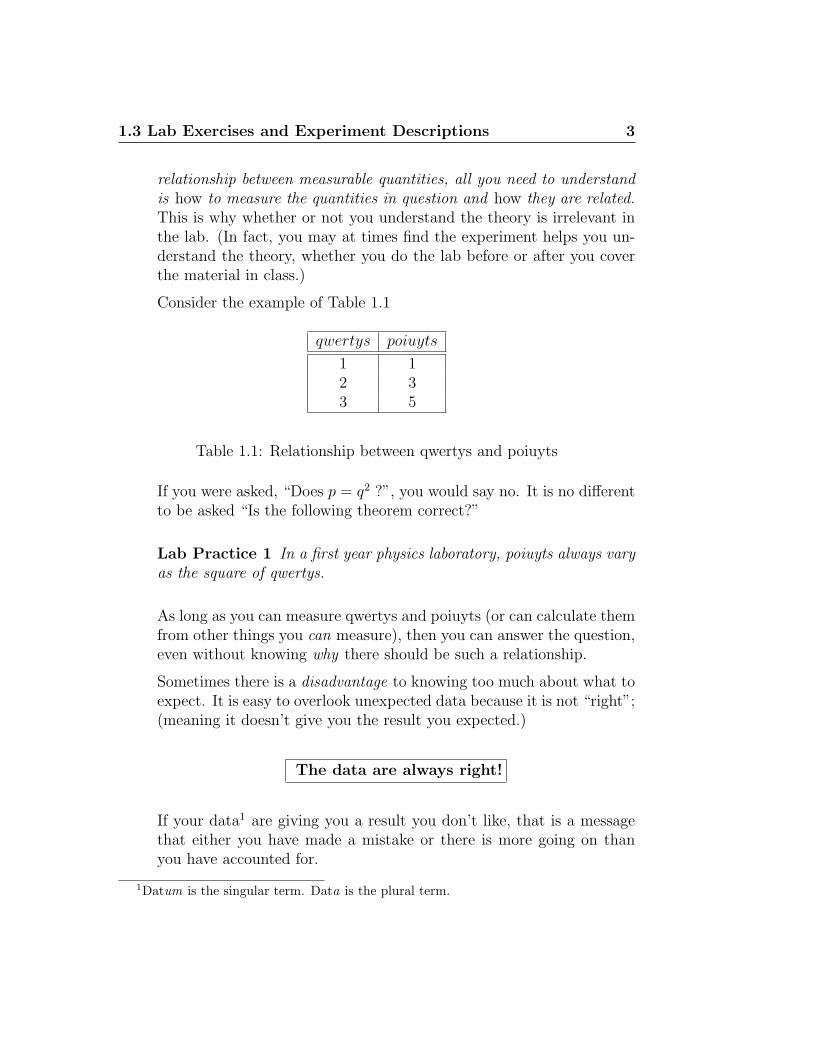
Consider the example of Table 1.1

qwertys poiuyts

1 12 33 5

Table 1.1: Relationship between qwertys and poiuyts

If you were asked, “Does p = q2 ?”, you would say no. It is no differentto be asked “Is the following theorem correct?”

Lab Practice 1 In a first year physics laboratory, poiuyts always varyas the square of qwertys.

As long as you can measure qwertys and poiuyts (or can calculate themfrom other things you can measure), then you can answer the question,even without knowing why there should be such a relationship.

Sometimes there is a disadvantage to knowing too much about what toexpect. It is easy to overlook unexpected data because it is not “right”;(meaning it doesn’t give you the result you expected.)

The data are always right!

If your data1 are giving you a result you don’t like, that is a messagethat either you have made a mistake or there is more going on thanyou have accounted for.

1Datum is the singular term. Data is the plural term.

4 Lab Manual Layout

• Procedure

This tells you what you are required to do to perform the experiment.Unless you are told otherwise, these instructions are to be followedprecisely. If there are any changes necessary, you will be informed inthe lab.

Questions will need to be handed in; tasks will be checked off in thelab.

Included in this section are three important subsections:

– Preparation (including pre-lab questions and tasks)

The amount of time spent in a lab can vary greatly dependingon what has been done ahead of time. This section attempts tominimize wasted time in the lab .

– Experimentation or Investigation

(including in-lab questions and tasks)

For some lab exercises, there won’t be an “experiment” as such,but there will be things to be done in the lab. The in-lab ques-tions can usually only be answered while you have access to the labequipment, but the answers will be important for further calcula-tions and interpretation. For computer labs, instead of questionsthere will often be tasks, consisting of points to be demonstratedwhile you are in the lab.

– Analysis (usually for labs) or Follow-up (usually for exercises)

(including post-lab questions and tasks)

Many of the calculations for a lab can be done afterward, providedyou understand clearly what you are doing in the lab, record allof the necessary data, and answer all of the in-lab questions. Thepost-lab questions summarize the important points which must beaddressed in the lab report.

Since most of the exercises are developing skills, the results canusually be applied immediately to labs either already begun orupcoming.

1.4 Templates 5

• Bonus

Most experiments will have a bonus question allowing you to take onfurther challenges to develop more understanding, either of data analy-sis concepts or of the underlying theory. (Bonus questions will usuallybe worth an extra 5% or so on the lab if they are done correctly.)

1.4 Templates

Each experiment, and many exercises, include a template. This is to helpyou ensure that you are not missing any data when you leave the lab. Sinceyou will perform many calculations outside the lab, you’ll need to make sureyou have everything you need before you leave.

1.4.1 Table format in templates and lab reports

The templates are set up to help you consistently record information. Forthat reason, the tables are very “generic”. It would be more concise to createtables that are specific to each experiment, but that would not be as helpfulfor your education. When you write a report, you should set up tables whichare concise and experiment-specific, even if they look different than the onesin the template.

Don’t automatically set up tables in your lab reports like the ones in thetemplates.

1.4.2 Template tables

• The first table contains information which you should record every timeyou do an experiment, and looks like this:

6 Lab Manual Layout

My name:My student number:My partner’s name:My partner’s student number:My other partner’s name:My other partner’s student number:My lab section:My lab demonstrator:Today’s date:

1.4.3 Before the lab

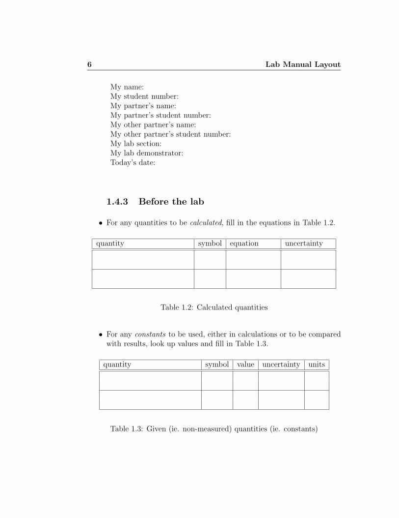
• For any quantities to be calculated, fill in the equations in Table 1.2.

quantity symbol equation uncertainty

Table 1.2: Calculated quantities

• For any constants to be used, either in calculations or to be comparedwith results, look up values and fill in Table 1.3.

quantity symbol value uncertainty units

Table 1.3: Given (ie. non-measured) quantities (ie. constants)

1.4 Templates 7

1.4.4 In the lab

• For any new measuring instruments, (ie. ones you have not used pre-viously), fill in the information in Table A.1 or Table A.2.

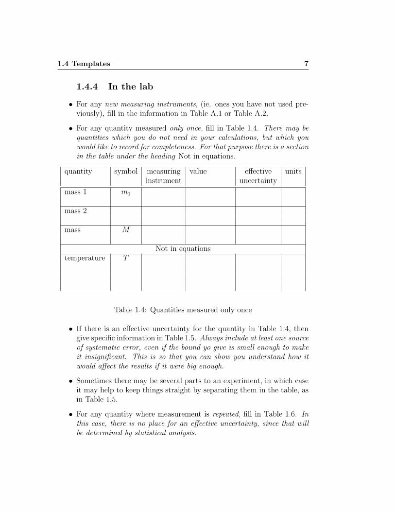
• For any quantity measured only once, fill in Table 1.4. There may bequantities which you do not need in your calculations, but which youwould like to record for completeness. For that purpose there is a sectionin the table under the heading Not in equations.

quantity symbol measuring value effective unitsinstrument uncertainty

mass 1 m1

mass 2

mass M

Not in equationstemperature T

Table 1.4: Quantities measured only once

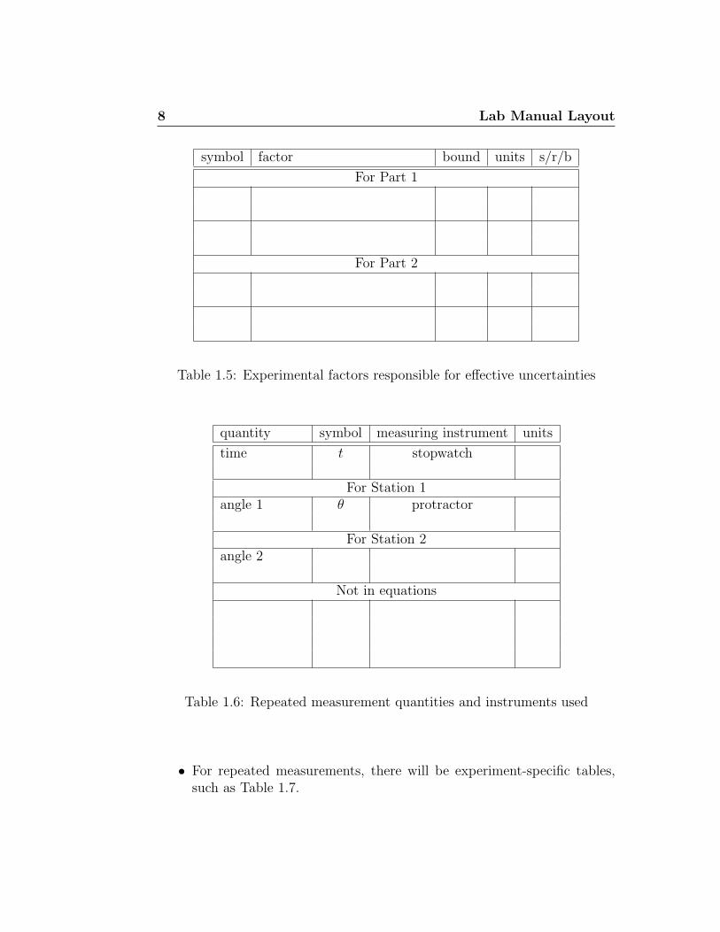
• If there is an effective uncertainty for the quantity in Table 1.4, thengive specific information in Table 1.5. Always include at least one sourceof systematic error, even if the bound yo give is small enough to makeit insignificant. This is so that you can show you understand how itwould affect the results if it were big enough.

• Sometimes there may be several parts to an experiment, in which caseit may help to keep things straight by separating them in the table, asin Table 1.5.

• For any quantity where measurement is repeated, fill in Table 1.6. Inthis case, there is no place for an effective uncertainty, since that willbe determined by statistical analysis.

8 Lab Manual Layout

symbol factor bound units s/r/b

For Part 1

For Part 2

Table 1.5: Experimental factors responsible for effective uncertainties

quantity symbol measuring instrument units

time t stopwatch

For Station 1angle 1 θ protractor

For Station 2angle 2

Not in equations

Table 1.6: Repeated measurement quantities and instruments used

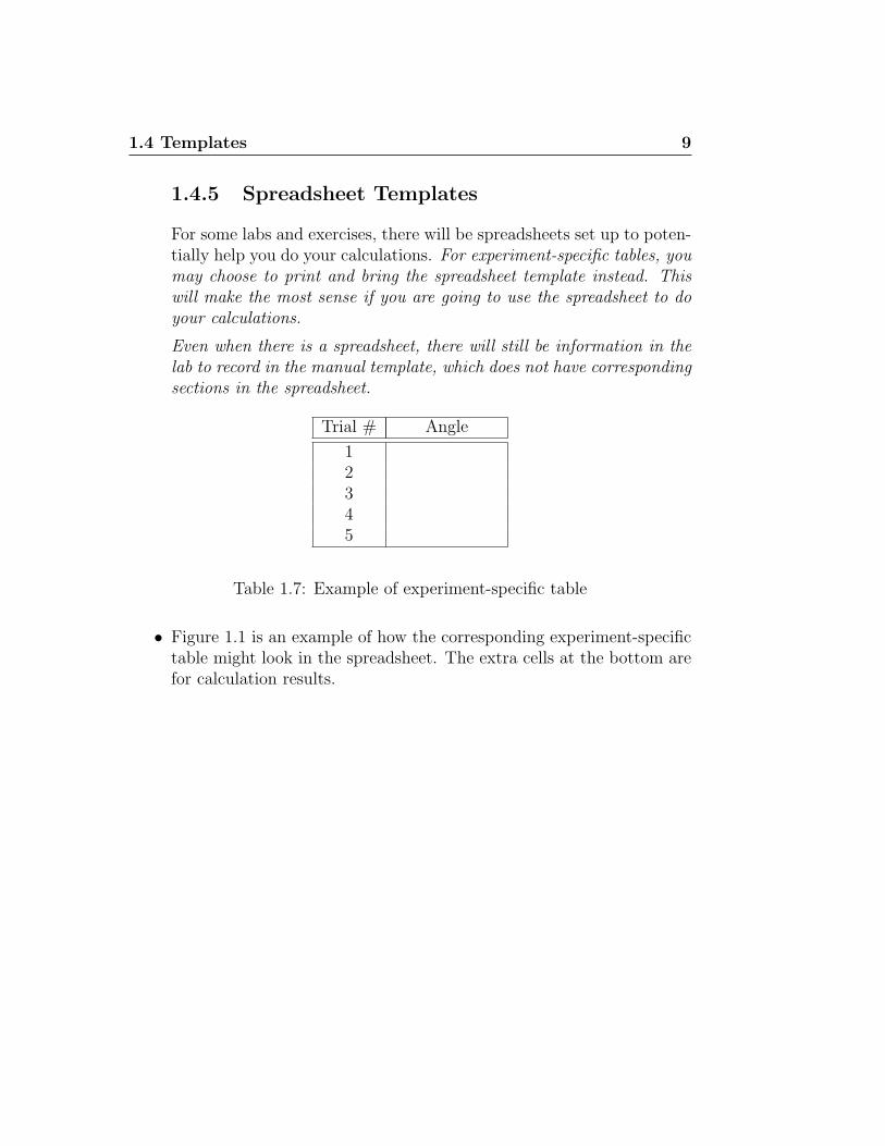
• For repeated measurements, there will be experiment-specific tables,such as Table 1.7.

1.4 Templates 9

1.4.5 Spreadsheet Templates

For some labs and exercises, there will be spreadsheets set up to poten-tially help you do your calculations. For experiment-specific tables, youmay choose to print and bring the spreadsheet template instead. Thiswill make the most sense if you are going to use the spreadsheet to doyour calculations.

Even when there is a spreadsheet, there will still be information in thelab to record in the manual template, which does not have correspondingsections in the spreadsheet.

Trial # Angle

12345

Table 1.7: Example of experiment-specific table

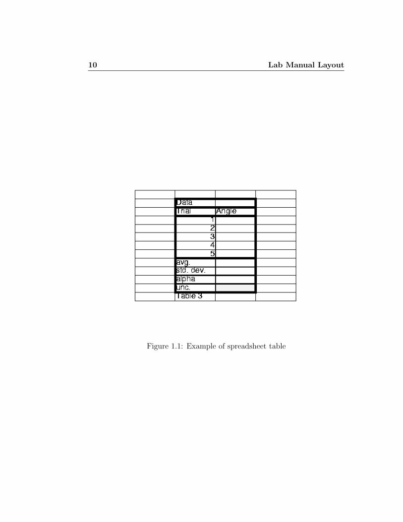
• Figure 1.1 is an example of how the corresponding experiment-specifictable might look in the spreadsheet. The extra cells at the bottom arefor calculation results.

10 Lab Manual Layout

Figure 1.1: Example of spreadsheet table

Chapter 2

Goals for PC131 Labs

When you take a science course, you are obviously going to learn some sci-ence. However, in a science course with labs, you are expected to learn howto think and act like a scientist, which is a different thing. It is like the dif-ference between being a spectator for a particular sport and actually beinga participant, or like the difference between enjoying cello music and play-ing the cello. Becoming a professional scientist (like becoming a professionalathlete or a professional musician) will require both learning science and howto think and act like a scientist. In the lectures for PC131, you will learn lotsof physics. In the labs, you will learn how to think and act as a physicist.

Usually, one thinks of the purpose of a lab as being the demonstration ortesting of laws of some sort, but a lab should accomplish more than that. Infact, learning how to demonstrate or test physical theories or laws is moreimportant (in the lab) than learning the laws themselves.

Learning the physics theory behind any particular experiment can bedone in a lecture, and so that is not the main focus of the lab. In fact,for some experiments the “theory” behind them may never be covered inclass. Part of what you should learn through your university career is howto assimilate knowledge. In other words, you are now going to begin to beexpected to learn things on your own. In the lab, this will originally amountto reading the lab manual ahead of time to get an idea of what you willbe doing in the lab. (Later in the course there may be more preparationrequired.) If you feel you need more information, you may need to look it upyourself.

As well, what you learn in the lab should be applicable in other areas ofstudy after you are finished this course. For example, you may never again

12 Goals for PC131 Labs

need to calculate the acceleration due to gravity, however, if you continue inscience you will be sure to do more data analysis of some type.

For these reasons, the labs in this course will be intended to address threemajor issues:

1. One has to understand what it means to test or demonstrate a lawbefore one can actually do so.

2. To actually perform an experiment, a student will often be required tobecome familiar with

(a) lab apparatus and equipment,

(b) measurement techniques and efficient methods of gathering data,

(c) methods and tools for data analysis.

3. The results of an experiment are only useful if they can be communi-cated to others.

For these reasons, the goals of the labs in this course will fall into thesegeneral areas:

• develop understanding of what it means to demonstrate or test physicallaws

• introduce measurement tools and equipment

• introduce measurement techniques

• introduce uncertainty (or error) analysis tools and techniques

• promote organized presentation of results in the format of formal labreports.

High school physics labs tend to focus mainly on the second of theseabove; in this course we will touch on all of them. It should become appar-ent that the second one is fairly experiment–dependent, whereas the othersare less so. While the specific theories tested and the format of the reportrequired may be unique to this course, it is important that you as a scientistdevelop the skills which allow you to investigate theories to assess their va-lidity and communicate your results in a clear and concise manner regardlessof your field of study.

Chapter 3

Instructions for PC131 Labs

Students will be divided into sections, each of which will be supervised by alab supervisor and a demonstrator. This lab supervisor should be informedof any reason for absence, such as illness, as soon as possible. (If the studentknows of a potential absence in advance, then the lab supervisor should beinformed in advance.) A student should provide a doctor’s certificate forabsence due to illness. Missed labs will normally have to be made up, andusually this will be scheduled as soon as possible after the lab which wasmissed while the equipment is still set up for the experiment in question.

It is up to the student to read over any theory for each experiment andunderstand the procedures and do any required preparation before the labora-tory session begins. This may at times require more time outside the lab thanthe time spent in the lab.

Students are normally expected to complete all the experiments assignedto them, and to submit a written report of your experimental work, includingraw data, as required.

You will be informed by the lab instructor of the location for submissionof your reports during your first laboratory period. This report will usuallybe graded and returned to you by the next session. The demonstrator whomarked a particular lab will be identified, and any questions about markingshould first be directed to that demonstrator. Such questions must be directedto the marker within one week of the lab being returned to the student if anyadditional marks are requested.

Unless otherwise stated, all labs and exercises will count toward your labmark, although they may not all carry equal weight. If you have questionsabout this talk to the lab supervisor.

14 Instructions for PC131 Labs

3.1 Expectations

As a student in university, there are certain things expected of you. Some ofthem are as follows:

• You are expected to come to the lab prepared. This means first of allthat you will ensure that you have all of the information you need todo the labs, including answers to the pre-lab questions. After you havebeen told what lab you will be doing, you should read it ahead andbe clear on what it requires. You should bring the lab manual, lecturenotes, etc. with you to every lab. (Of course you will be on time soyou do not miss important information and instructions.)

• You are expected to be organized This includes recording raw data withsufficient information so that you can understand it, keeping properbackups of data, reports, etc., hanging on to previous reports, and soon. It also means starting work early so there is enough time to clarifypoints, write up your report and hand it in on time.

• You are expected to be adaptable and use common sense. In labs itis often necessary to change certain details (eg. component values orprocedures) at lab time from what is written in the manual. You shouldbe alert to changes, and think rationally about those changes and reactaccordingly.

• You are expected to value the time of instructors and lab demonstrators.This means that you make use of the lab time when it is scheduled,and try to make it as productive as possible. This means NOT arrivinglate or leaving early and then seeking help at other times for what youmissed.

• You are expected to act on feedback from instructors, markers, etc. Ifyou get something wrong, find out how to do it right and do so.

• You are expected to use all of the resources at your disposal. This in-cludes everything in the lab manual, textbooks for other related courses,the library, etc.

• You are expected to collect your own data. This means that you per-form experiments with your partner and no one else. If, due to an

3.2 Workload 15

emergency, you are forced to use someone else’s data, you must explainwhy you did so and explain whose data you used. Otherwise, you arecommitting plagiarism.

• You are expected to do your own work. This means that you prepareyour reports with no one else. If you ask someone else for advice aboutsomething in the lab, make sure that anything you write down is basedon your own understanding. If you are basically regurgitating someoneelse’s ideas, even in your own words, you are committing plagiarism.(See the next point.)

• You are expected to understand your own report. If you discuss ideaswith other people, even your partner, do not use those ideas in yourreport unless you have adopted them yourself. You are responsible forall of the information in your report.

• You are expected to be professional about your work. This meansmeeting deadlines, understanding and meeting requirements for labs,reports, etc. This means doing what should be done, rather than whatyou think you can get away with. This means proofreading reports forspelling, grammar, etc. before handing them in.

• You are expected to actively participate in your own education. Thismeans that in the lab, you do not leave tasks to your partner becauseyou do not understand them. This means that you try and learn howand why to do something, rather than merely finding out the result ofdoing something.

3.2 Workload

Even though the labs are each only worth part of your course mark, theamount of work involved is probably disproportionately higher than for as-signments, etc. Since most of the “hands-on” portion of your education willoccur in the labs, this should not be surprising. (Note: skipping lectures orlabs to study for tests is a very bad idea. Good time management is a muchbetter idea.)

16 Instructions for PC131 Labs

3.3 Administration

1. Students will be required to have a binder to contain all lab manualsections and all lab reports which have been returned. (A 3 hole punchwill be in the lab.)

2. Templates will be used in each experiment as follows:

(a) The template must be checked and initialed by the demonstratorbefore students leave the lab.

(b) No more than 3 people can use one set of data. If equipment istight groups will have to split up. (ie. Only as many people as fitthe designated places for names on a template may use the samedata.)

(c) 5% of the lab mark will be for the template.

(d) The template must be included with lab handed in. (A 5% penaltywill be incurred if it is missing.) It must be the original, not aphotocopy.

(e) Missing a lab without a doctor’s note gives up the template markand marks for question answers.

(f) If a student misses a lab, and if space permits (decided by thelab supervisor) the student may do the lab in another section thesame week without penalty. (However the due date is still for thestudent’s own section.) In that case the section recorded on thetemplate should be where the experiment was done, not where thestudent normally belongs.

3. In-lab tasks must be checked off before the end of the lab, and answersto in-lab questions must be handed in at the end of the lab. Students areto make notes about question answers and keep them in their bindersso that the points raised can be discussed in their reports. Marks foranswers to questions will be added to marks for the lab. For peoplewho have missed the lab without a doctor’s note and have not made upthe lab, these marks will be forfeit. The points raised in the answerswill still be expected to be addressed in the lab report.

4. Labs handed in after the due date incur a penalty of 5% per day late toa maximum penalty of 50%. After the reports for an experiment have

3.4 Plagiarism 17

been returned, any late reports submitted for that experiment cannotreceive a grade higher than the lowest mark from that lab section forthe reports which were submitted on time.

3.4 Plagiarism

5. Plagiarism includes the following:

• Identical or nearly identical wording in any block of text.

• Identical formatting of lists, calculations, derivations, etc. whichsuggests a file was copied.

6. You will get one warning the first time plagiarism is suspected. Afterthis any suspected plagiarism will be forwarded directly to the courseinstructor. With the warning you will get a zero on the relevant sec-tion(s) of the lab report. If you wish to appeal this, you will have todiscuss it with the lab supervisor and the course instructor.

7. If there is a suspected case of plagiarism involving a lab report of yours,it does not matter whether yours is the original or the copy. Thesanctions are the same.

3.5 Calculation of marks

8. All of the labs and exercises will count toward your average. Exerciseswill count less than labs.

9. The weighting of individual labs and exercises may depend on the qual-ity of the work; ie. if you do better work on some things they will countmore toward your final grade. Details will be discussed in the lab.

10. There may be a lab test at the end of term.

18 Instructions for PC131 Labs

Chapter 4

How To Prepare for a Lab

“The theory section for an experiment should give any math-ematical relationship(s) pertinent to that experiment, along withany definitions, etc. which may be needed. You don’t have tounderstand a theory in depth to test it; inasmuch as it is a math-ematical relationship between measurable quantities all you needto understand is how to measure the quantities in question andhow they are related. This is why whether or not you understandthe theory is irrelevant in the lab. (In fact, you may at times findthe experiment helps you understand the theory, whether you dothe lab before or after you cover the material in class.)”

1. Check the web page after noon on the Friday before the lab to makesure of what you need to bring, hand in, etc. (It is a good idea to checkthe web page the day of your lab, in case there are any last minutecorrections to the instructions.)

2. Read over the lab write–up to determine what the physics is behindit. (Even without understanding the physics in detail, you can do allof the following steps.)

3. Answer all of the pre-lab questions and do all of the pre-lab tasks andbring the answers with you to the lab.

4. Examine the spreadsheet and/or template for the lab (if either of themexists) to be sure that you understand what all of the quantities, sym-bols, etc. mean. (If there is a spreadsheet, you can prepare any or allof the formulas before the lab to simplify analysis later.)

20 How To Prepare for a Lab

5. Enter any constants into the appropriate table(s) in the template.

6. Highlight all of the in-lab questions and tasks so you can be sure toanswer them all in the lab.

7. Check the web page the day of the lab in case there are any last minutechanges or corrections to previous instructions.

8. Arrive on time, prepared. Bring all previous labs, calculator, and any-thing else which might be of use. (If the theory is in your textbook,maybe it would be good to bring your textbook to the lab!)

Chapter 5

Plagiarism

5.1 Plagiarism vs. Copyright Violation

These two concepts are related, but may get confused. Both involve unethicalre-use of one person’s work by another person, but they are different becausethe victim is different in each case.

Copyright is the right of an author to control over the publication ordistribution of his or her own work. A violation of copyright is, in effect, acrime against the producer of the work, since adequate credit and/or paymentis not given.

Plagiarism is the presentation of someone else’s work as one’s own, andthus the crime is against the reader or recipient of the work who is beingdeceived about its source.

Putting these two together suggests that there is a great deal of overlap,since trying to pass off someone else’s work without that person’s permis-sion as one’s own is both plagiarism and a violation of copyright. However,copying someone else’s work without permission, even without denying whoproduced it, is still a violation of copyright. Conversely, presenting someoneelse’s work as your own, even with that person’s permission,is still plagiarism.

5.2 Plagiarism Within the University

The Wilfrid Laurier University calendar says: “ plagiarism . . . is the unac-knowledged presentation, in whole or in part, of the work of others as one’s

22 Plagiarism

own, whether in written, oral or other form, in an examination, report, as-signment, thesis or dissertation ”

A search of the university web site for the word “plagiarism” turns upseveral things, among them the following:

• “Of course, under no circumstance is it acceptable to directly use anauthor’s words (or a variation with only a few words of a sentencechanged) without giving that author credit; this is plagiarism!!!” (Psy-chology 229)

• “plagiarism, which includes but is not limited to: the unacknowledgedpresentation, in whole or in part, of the work of others as one’s own;the failure to acknowledge the substantive contributions of academiccolleagues, including students, or others; the use of unpublished mate-rial of other researchers or authors, including students or staff, withouttheir permission;” (Faculty Association Collective Agreement)

• “DO NOT COPY DOWN A SECTION FROM YOUR SOURCE VER-BATIM OR WITH VERY MINOR CHANGES. This is PLAGIARISMand can lead to severe penalties. Obviously,no instructor can catch alloffenders but, to paraphrase the great Clint Eastwood, “What you needto ask yourself is ‘Do I feel lucky today?’ ” (Contemporary Studies100 Notes on Quotes)

• “Some people seem to think that if they use someone else’s work, butmake slight changes in wording, then all they need to do is make ref-erence to the “other” work in the standard way, i.e., (Smith, 1985),and there is no plagiarism involved. This is not true. You must ei-ther use direct quotes (with full references, including page numbers)or completely rephrase things in your own words (and even here youmust fully reference the original source of the idea(s)).” (Psychology306, quote from Making sense in psychology and the life sciences: Astudent’s guide to writing and style , by Margot Northey and BrianTimney (Toronto: Oxford University Press, 1986, pp. 32-33).)

• “Any student who has been caught submitting material that is notproperly referenced, where appropriate, or submits material that iscopied from another source (either a text or another student’s lab),

5.3 How to Avoid Plagiarism 23

will be subject to the penalties outlined in the Student Calendar.”(Geography 100)

• “Paraphrasing means restating a passage of a text in your own words,that is, rewording the ideas of someone else. In such a case, properreference to the author must be given, or it is plagiarism. Copying apassage verbatim (not paraphrased) also constitutes plagiarism if it isnot placed in quotes and is not referenced. Plagiarism is the appro-priation or imitation of the language, ideas, and thoughts of anotherauthor, and the representation of these as one’s own.” (Biology 100)

5.3 How to Avoid Plagiarism

Plagiarism is a serious offense, and will be treated that way, but often stu-dents are unclear about what it is. The above quotes should help, but hereare some more guidelines:

• If you use the same data as anyone else, this should be clearly doc-umented in your report, WHETHER THE DATA ARE YOURS ORTHEIRS.

• If you copy any file, even if you modify it, it is plagiarism unless youclearly document it. (This does not mean you can copy whatever youlike as long as it’s documented; you still are expected to do your ownwork. However at least you’re not plagiarizing if you document yoursources properly.)

• You are responsible for anything in your report; if you answer a questionabout your report with, “I don’t know, my partner did that part”, youare guilty of plagiarism, because you are passing off your partner’s workas your own.

• The purpose for working together is to help each other learn. If collab-oration is done in order for one or more people to avoid having to learnand/or work, then it is very likely going to involve plagiarism, (and isa no-no for pedagogical reasons anyway.)

• If you give your data, files, etc. to anyone else and they plagiarizeit you are in trouble as well, because you are aiding their attempt to

24 Plagiarism

cheat. Do not give out data, files, or anything else without expresspermission from the lab supervisor. This includes giving others yourwork to “look at”; if you give it to them, for whatever reason, and theycopy it, you have a problem.

• If you want to talk over ideas with others, do not write while you arediscussing; if everyone is on their own when they write up their reports,then the group discussion should not be a problem. However, as in aprevious point, do not use group consensus as justification for what youwrite; discussion with anyone else should be to help you sort out yourthoughts, not to get the “right answers” for you to parrot.

Look at the following from the writing centre, “How to Use Sources andAvoid Plagiarism”

< http : //www.wlu.ca/ ∼ wwwwc/handouts/sources.htm >

Chapter 6

Lab Reports

A lab report is personal, in the sense that it explains what you did in the laband summarizes your results, as opposed to an assignment which generallyanswers a question of some sort. On an assignment, there is (usually) a “rightanswer”, and finding it is the main part of the exercise. In a lab report, ratherthan determining an “answer”, you may be asked to test something. (Notethat no experiment can ever prove anything; it can only provide evidence foror against; just like in mathematics finding a single case in which a theoremholds true does not prove it, although a single case in which it does not holdrefutes the theorem. A law in physics is simply a theorem which has beentested countless times without evidence of a case in which it does not hold.)The point of the lab report, when testing a theorem or law, is to explainwhether or not you were successful, and to give reasons why or why not. Inthe case where you are to produce an “answer”, (such as a value for g), youranswer is likely to be different from that of anyone else; your job is to describehow you arrived at yours and why it is reasonable under the circumstances.

6.1 Format of a Lab Report

The format of the report should be as follows:

6.1.1 Title

The title should be more specific than what is given in the manual; it shouldreflect some specifics of the experiment.

26 Lab Reports

6.1.2 Purpose

The specific purpose of the experiment should be briefly stated. (Note thatthis is not the same as the goals of the whole set of labs; while the labs as agroup are to teach data analysis techniques, etc., the specific purpose of oneexperiment may indeed be to determine a value for g, for instance.) Usually,the purpose of each experiment will be given in the lab manual. However, itwill be very general. As in the title, you should try and be a bit more specific.

There should always be both qualitative and quantitative goals for alab.

Qualitative

This would include things like “see if the effects of friction can be observed”.In order to achieve this, however, specific quantitative analyses will need tobe performed.

Quantitative

In a scientific experiment, there will always be numerical results producedwhich are compared with each other or to other values. It is based on the re-sults of these comparrisons that the qualitative interpretations will be made.

6.1.3 Introduction

In general, in this course, you will not have to write an Introduction section.

An introduction contains two things: theory for the experiment and ra-tionale for the experiment.

Theory

Background and theoretical details should go here. Normally, detailed deriva-tions of mathematical relationships should not be included, but referencesmust be listed. All statements, equations, and ‘accepted’ values must be jus-tified by either specifying the reference(s) or by derivation if the equation(s)cannot be found in a reference.

6.1 Format of a Lab Report 27

Rationale

This describes why the experiment is being done, which may include refer-ences to previous research, or a discussion of why the results are importantin a broader context.

6.1.4 Procedure

The procedure used should not be described unless you deviate from thatoutlined in the manual, or unless some procedural problem occurred, whichmust be mentioned. A reference to the appropriate chapter(s) of the labmanual is sufficient most of the time.

Ideally, someone reading your report and having access to the lab manualshould be able to reproduce your results, within reasonable limits. (Later onwe will discuss what “reasonable limits” are.) If you have made a mistake indoing the experiment, then your report should make it possible for someoneelse to do the experiment without making the same mistake. For this reason,lab reports are required to contain raw data, (which will be discussed later),and explanatory notes.

Explanatory notes are recorded to

• explain any changes to the procedure from that recorded in the labmanual,

• draw attention to measurements of parameters, values of constants, etc.used in calculations, and

• clarify any points about what was done which may otherwise be am-biguous.

Although the procedure need not be included, your report should be clearenough that the reader does not need the manual to understand your write–up.

(If you actually need to describe completely how the experiment was done,then it would be better to call it a “Methods” section, to be consistent withscientific papers.)

6.1.5 Experimental Results

There are two main components to this section; raw data and calculations.

28 Lab Reports

Raw Data

In this part, the reporting should be done part by part with the numberingand titling of the parts arranged in the same order as they appear in themanual.

The raw data are provided so that someone can work from the actualnumbers you wrote down originally before doing calculations. Often mistakesin calculation can be recognized and corrected after the fact by looking atthe raw data.

In this section:

• Measurements and the names and precision measures of all instrumentsused should be recorded; in tabular form where applicable.

• If the realistic uncertainty in any quantity is bigger than the precisionmeasure of the instrument involved, then the cause of the uncertaintyand a bound on its value should be given.

• Comments, implicitly or explicitly asked for regarding data, or exper-imental factors should be noted here. This will include the answeringof any given in-lab questions.

Calculations

There should be a clear path for a reader from raw data to the final resultspresented in a lab report. In this section of the report:

• Data which is modified from the original should be recorded here; intabular form where applicable.

• Uncertainties should be calculated for all results, unless otherwise spec-ified. The measurement uncertainties used in the calculations shouldbe those listed as realistic in the raw data section.

• Calculations of quantities and comparisons with known relationshipsshould be given. If, however, the calculations are repetitive, only onesample calculation, shown in detail, need be given. Error analysisshould appear here as well.

6.1 Format of a Lab Report 29

• Any required graphs would appear in this part. (More instructionabout how graphs should be presented will be given later.)

• For any graph, a table should be given which has columns for the data(including uncertainties) which are actually plotted on the graph.

• Comments, implicitly or explicitly asked for regarding calculations, ob-servations or graphs, should be made here. This will include answeringof any given post-lab questions.

Sample calculations may be required in a particular order or not. Ifthe order is not specified, it makes sense to do them in the order in whichthe calculations would be done in the experiment. If the same data can becarried through the whole set of calculations, that would be a good choice toillustrate what is happening.

Printing out a spreadsheet with formulas shown does not count as showingyour calculations; the reader does not have to be familiar with spreadsheetsyntax to make sense of results.

6.1.6 Discussion

This section is where you explain the significance of what you have deter-mined and outline the reasonable limits which you place on your results.(This is what separates a scientific report from an advertisement.) It shouldoutline the major sources of random and systematic error in an experiment.Your emphasis should be on those which are most significant, and on whichyou can easily place a numerical value. Wherever possible, you should tryto suggest evidence as to why these may have affected your results, and in-clude recommendations for how their effects may be minimized. This can beaccompanied by suggested improvements to the experiment.

Two extremes in tone of the discussion should be avoided: the first isthe “sales pitch” or advertisement mentioned above, and the other is the“apology” or disclaimer (“ I wouldn’t trust these results if I were you; they’reprobably hogwash.”) Avoid whining about the equipment, the time, etc. Yourjob is to explain briefly what factors most influenced your results, not to ab-solve yourself of responsibility for what you got, but to suggest changes orimprovements for someone attempting the same experiment in the future.

30 Lab Reports

Emphasis should be placed on improving the experiment by changed tech-nique, (which may be somewhat under your control), rather than by changedequipment, (which may not).

This section is usually worth a large part of the mark for a lab so beprepared to spend enough time thinking to do a reasonable job of it.

You must discuss at least one source of systematic error in your report, evenif you reject it as insignificant, in order to indicate how it would affect theresults.

6.1.7 Conclusions

Just as there are always both qualitative and quantitative goals for a lab,there should always be both qualitative and quantitative conclusions froma lab.

Qualitative

This would include things like “see if the effects of friction can be observed”.In order to achieve this, however, specific quantitative analyses will need tobe performed.

Quantitative

In a scientific experiment, there will always be numerical results producedwhich are compared with each other or to other values. It is based on the re-sults of these comparrisons that the qualitative interpretations will be made.

General comments regarding the nature of results and the validity of rela-tionships used would be given in this section. Keep in mind that these com-ments can be made with certainty based on the results of error calculations.The results of the different exercises should be commented on individually.Your conclusions should refer to your original purpose; eg. if you set out todetermine a value for g then your conclusions should include your calculatedvalue of g and a comparison of your value with what you would expect.

While you may not have as much to say in this section, what you sayshould be clear and concise.

6.2 Final Remarks 31

6.1.8 References

If an ‘accepted’ value is used in your report, then the value should be foot-noted and the reference given in standard form. Any references used for thetheory should be listed here as well.

6.2 Final Remarks

Reports should be clear, concise, and easy to read. Messy, unorganizedpapers never fail to insult the reader (normally the marker) and your gradewill reflect this. A professional report, in quality and detail, is at least asimportant as careful experimental technique and analysis.

Lab reports should usually be typed so that everything is neat and or-ganized. Be sure to spell check and watch for mistakes due to using wordswhich are correctly spelled but inappropriate.

6.3 Note on Lab Exercises

Lab exercises are different than lab reports, and so the format of the write-up is different. Generally exercises will be shorter, and they will not includeeither a Discussion or a Conclusion section.

Computer lab exercises may require little or even no report, but will havepoints which must be demonstrated in the lab.

32 Lab Reports

Chapter 7

Measurement and Uncertainties

If it’s green and wiggles, it’s biology;If it stinks, it’s chemistry;If it doesn’t work, it’s physics.1

The quote above is rather cynical, but depending on what is meant by“work”, there may be some truth to it. In physics most of the numbersused are not exact but only approximate. These approximate numbers arisefrom two principal sources:

1. uncertainties in individual measurements

2. reproducibility of successive measurements of the same quantities.

The first of these cases will be discussed in the following section, while thesecond will be discussed somewhat here, and more later.

7.1 Errors and Uncertainties

When an experiment is performed, every effort is made to ensure that what isbeing measured is what is supposed to be measured. Factors which hinder thisare called experimental errors, and the existence of these factors resultsin uncertainty in quantities measured.

1The Physics Teacher 11, 191 (1973)

34 Measurement and Uncertainties

7.2 Single Measurement Uncertainties

When a number is obtained as a measure of length, area, angle, or otherquantity, its reliability depends on the precision2 of the instrument used,the repeatability of the measurement, the care taken by the experimenter,and on the subjectivity of the measurement itself.

7.2.1 Expressing Quantities with Uncertainties

Consider a measured length that is found to be between 14.255 cm and14.265 cm. A number like this should be recorded as 14.260± 0.005 cm,where the 0.005 cm is the uncertainty 3 in the length.

Note: Digits which are not stated are definitely uncertain. They are, infact, unknown, and you can’t get any more uncertain than that! For instance,it makes no sense to quote a value of 78.3±0.0003kg. Unless the next threedigits after the decimal place are known to be zeroes, then the uncertaintydue to those unknown digits is much bigger than 0.0003kg. If we actuallymeasured a value of 78.3000kg, then those zeroes should be stated, otherwiseour uncertainty is meaningless. (More will be said about significant figureslater.)

Remember: The uncertainty in a measurement should always be in the lastdigit quoted; ie. the least significant digit recorded is the uncertain one.

7.2.2 Random and Systematic Errors

There are two main categories for errors, (ie. sources of uncertainty), whichcan occur: systematic and random.

• Systematic errors are those which, if present, will skew the results ina particular direction, and possibly by a relatively consistent amount.For instance, If we need to calculate the volume of the inside of a tube,and we measure the outer dimensions of the tube, then the volume wecalculate will be a little higher than it should be. If we repeated the

2This term will be discussed in detail later.3The term error is also used for uncertainty, but it suggests the idea of mistakes, and

so it will be avoided where possible, except to describe the experimental factors whichlead to the uncertainty.

7.2 Single Measurement Uncertainties 35

measurement a few times, we might get slightly different results, butthey would all be high.

• Random errors, on the other hand, cannot be consistently predicted, indirection or size, outside of perhaps broad limits. For example, if youare trying to measure the average diameter of a sample of ball bearings,then if they are randomly chosen there is no reason to assume that thefirst one measured will be either above average or below.

One of the important differences between random and systematic errorsis that systematic errors can be corrected for after the fact, if they can bebounded. (If we measured the thickness of the walls of the tube from theexample above, we could use this to correct the volume.) Random errors canonly be reduced by repeating the number of measurements. (This will bediscussed later.)

It should be noted that a particular measurement may combine bothtypes of errors; if the two above examples are combined, so that one is tryingto determine the average inner volume of a bunch of tubes by measuringthe outer dimensions, then there would be a systematic error, (due to thedifference between inner and outer dimensions), and a random error, (due tothe variation between the tubes), which would both affect the results.

7.2.3 Recording Precision with a Measurement

When taking measurements, one can usually estimate a reading to the nearest1/2 of the smallest division marked on the scale. This quantity is known asthe precision measure of the instrument. For a digital device, you canmeasure to the least significant digit.

So, for example, if a metre stick has markings every millimetre, then theprecision measure is 0.5 mm, and all measurements should be to 10ths ofmillimetres. On the other hand, if a digital stopwatch measures to 1/100thof a second, the precision measure is 0.01s and measurements should be tohundredths of seconds.

Determine the precision measure of an instrument before taking any mea-surements, not after. Since the number of digits you quote will depend onthe precision measure, you cannot make them up after the fact, or assumethem to be zero.

36 Measurement and Uncertainties

7.2.4 Realistic Uncertainties

Sometimes the precision you can actually achieve in a measurement is lessthan what is theoretically possible. In other words, your uncertainty is notdetermined by the precision measure of the instrument, but is somewhatlarger because of other factors.

The size of the uncertainty you quote should reflect the real range of possiblevalues for the quantity measured. You should be prepared to defend anymeasurement within the uncertainty you give for it, so do not blithely quotethe precision measure of the instrument as the uncertainty unless you areconvinced that it is appropriate. The precision measure is the best that youcan do with an instrument; the uncertainty you quote should be what youcan realistically do. Your goal as you do the experiment is to try and reduceother factors as much as possible so that you can get as close to the precisionmeasure as possible.

There are many possible sources for the uncertainty in a single quan-tity which all contribute to the total uncertainty. The magnitude of eachuncertainty contribution can vary, and the uncertainty you quote with themeasurement should take all of the sources into account and be realistic. Forinstance, suppose you measure the length of a table with a metre stick. Theuncertainty in the length will come from several sources, including:

• the precision measure of the metre stick

• the unevenness of the ends of the table

• the unevenness of the top of the table (or the side, if you place themetre stick alongside the table to measure)

• the temperature of the room (a metal metre stick will expand or con-tract)

• the humidity of the room (a wooden table and/or metre stick will swellor shrink)

It is possible to come up with many other sources of uncertainty, but it shouldbe clear that this does not make the uncertainty you use arbitrarily large.In this example, you’d probably ultimately believe your measurement to bewithin a cm or so, no matter what, and so that is the uncertainty you should

7.2 Single Measurement Uncertainties 37

use. (On the other hand, your uncertainty should not be unrealisticallysmall. Even if the metre stick has a precision measure of say, one millimetre,your uncertainty is obviously bigger than that if the ends of the table havevariations of 3 or 4 millimetres from one side of the table to the other.)

Usually if the uncertainty in a quantity is bigger than the precision measure,it will be due mainly to a single factor, or perhaps a couple of factors. It israre that there will be several errors equally contributing to the uncertaintyin a single quantity.

Repeatability of Measurements

Whether we repeat a measurement or not, its realistic uncertainty shouldreflect how close we would be able to be if we attempted to repeat the exper-iment. This reflects many things, including the strictness of our definitionof what we are measuring. A later section of the lab manual, Chapter 8,“Repeated Independent Measurement Uncertainties”, will discuss how to cal-culate the uncertainty if we are actually able to repeat a measurement severaltimes.

Here’s a guideline for determining the size of the “realistic uncertainty” in aquantity: If someone was to try and repeat your measurement, with only theinstructions you have written about how the measurement was made, howbig a discrepancy could they reasonably have from the value you got?

Subjectivity

Suppose you are measuring the distance between two dots on a page witha ruler. If the ruler has a precision measure of 0.5mm, but the dots arenon-uniform “blobs” which are several millimetres wide, then your effectiveuncertainty is going to be perhaps a few millimeters. The subjectivity indetermining the centre of the blobs is responsible for this. When you findyourself in this situation, you should note why you must quote a larger un-certainty than might be expected, and how you have determined its value.

38 Measurement and Uncertainties

7.2.5 Zero Error

Some measuring instruments have a certain zero error associated with them.This is the actual reading of the instrument when the expected value wouldbe zero. For instance, if a spring scale reads 5g with no weight hanging onit, then it has a zero error of 5g. Any measurement made will thus be 5g toohigh, and so 5g must be subtracted from any measurements. (If the zero errorwas minus 5g, then 5g would have to be added to every subsequent measure-ment. Always be sure to check and record the zero error of an instrumentwith its uncertainty. (Since the zero error is itself a measurement, then it hasan uncertainty just like any other measurement.) Subsequent measurementswith that instrument should be corrected by adding or subtracting the zeroerror as appropriate.

With some very sensitive digital instruments, there may be another factor:if the “zero” value of the scale fluctuates over time, then the fluctuationshould be taken into account.

7.3 Precision and Accuracy

Two concepts which arise in the discussion of experimental errors are preci-sion and accuracy which, in general, are not the same thing.

7.3.1 Precision

Precision refers to the number of significant digits and/or decimal placesthat can be reliably determined with a given instrument or technique. Theprecision of a quantity is revealed by its uncertainty.Precision (or uncertainty) can be expressed as either absolute or relative. Inthe first case, it will have the same units as the quantity itself; in the latter,it will be given as a proportion or a percentage of the quantity.

Uncertainties may be expressed in the first manner, ( i.e. having units),are called absolute uncertainties. Uncertainties be expressed as a percent-age of a quantity are then called percentage uncertainties.

For example, the measurement of the diameter of two different cylinderswith a meter stick may yield the following results:

d1 = 0.10±0.05cm

d2 = 10.00±0.05cm

7.3 Precision and Accuracy 39

Clearly, both measurements have the same absolute precision of 0.05 cm, i.e.,the diameters can be determined reliably to within 0.5 millimeters, but therelative precisions are quite different. For d1, the relative precision is

0.05

0.10× 100% = 50.0%

whereas for d2 it is0.05

10.00× 100% = 0.5%

so we could express these two quantities as

d1 = 0.10± 50.0%

d2 = 10.00± 0.5%

An error which amounts to a half a percent in the overall diameter is probablynot worth quibbling about, but a fifty percent error is highly significant.Consequently, we would say that the measurement of d2 is more precise thanthe measurement of d1. The relative precision tells us immediately thatthere is something wrong with the first measurement, namely, we are usingthe wrong instrument. Something more precise is needed, like a micrometeror vernier calipers, where the precision may be more like ±0.0005 cm.

When comparing quantities, the more precise value is the one with thesmaller uncertainty.

7.3.2 Accuracy

Accuracy refers to how close the measured value is to the ‘true’ or correctvalue. Thus, if a steel bar has been carefully machined so that its lengthis 10.0000 ± 0.0005 cm, and you determine its length to be 11.00 ± 0.05cm, your measurement is precise, but inaccurate. On the other hand, ifyour measurement is 10.0 ± 0.5 cm, it is accurate, but imprecise, and ameasurement of the length which yields a value of 10.001 ± 0.005 cm canbe considered to be accurate and precise. Errors in precision and errors inaccuracy arise from very different causes, as we shall discuss in the nextsection.

If you do not know what value to “expect” for a quantity, then youcannot determine the accuracy of your result. This will sometimes be the

40 Measurement and Uncertainties

case. However, even in these cases, you will often still be able to use commonsense to determine whether a value is plausible. For instance, if you measuredthe mass of a marble to be 21kg, you should realize that is unreasonable. Ifyou get a value which is unreasonable, you should try and figure out why.(In this case, it may be that the mass should be 21 grams ; incorrect unitsare a common source of odd results.)

When comparing quantities, the more accurate value is the one which iscloser to the “correct” or expected value.

Systematic errors affect the accuracy of a measurement or result, while ran-dom errors affect the precision of a measurement or result.

7.4 Significant Figures

The approximate number 14.26 is said to be correct to 4 figures, or to have4 figure accuracy. Those figures that are known with reasonable accuracyare called significant figures. It is permissible to retain only one estimatedfigure in a result and this figure is also considered significant.

If three numbers are measured to be 327, 4.02, and 0.00268 respectively,they are each said to have three significant digits. Thus, in counting signifi-cant figures, the decimal place is disregarded. Zeros at the end of a numberare significant unless they are merely place holders. If, for example, a massis found to be 3.20 grams, the zero is significant. On the other hand, whenthe distance to the sun is given to be 150,000,000 km, this is consideredto have only 2 significant digits. Note that there is some ambiguity aboutthe significance of the trailing zeros in this case. This can be avoided bythe use of scientific notation, which for the above measurement would be1.5× 108 km. (Note that in this case, zeros are never place holders, and so,if shown, are always significant.) The following rules tell us which digits aresignificant in an approximate number:

1. all digits other than zero are significant

2. zeros between non–zero digits are significant

3. leading zeros in a number are not significant

7.4 Significant Figures 41

4. trailing zeros in a number may or may not be significant. Use thestandard form when appropriate to avoid any confusion of this type.

7.4.1 Significant Figures in Numbers with Uncertain-ties

When quantities have uncertainties, they should be written so that the un-certainty is given to one significant digit, and the the least significant digit ofthe quantity is the uncertain one. Thus, if a mass is measured to be 152.1gwith an uncertainty of 3.5g, then the quantity should be written as

152± 4g

(Note the “2” is the uncertain digit.)

When using scientific notation, you should separate the power of ten fromboth the quantity and its uncertainty to make it easier to see that this rulehas been followed. This is known as the standard form. Use the standardform when the quantities you are quoting have placeholder zeroes. Whenthey don’t, the standard form is unnecessary and a bit cumbersome. Ifyou are using the standard form correctly, it should allow you to presentresults with uncertainties more concisely. Any time that it would be shorterto present a result without using the standard form, it should not be used.

For instance, if the speed of light was measured to be 2.94×108m/s withan uncertainty of 6.3× 106m/s, then it should be written as

c = (2.94± 0.06)× 108m/s

Note that this makes the relative uncertainty easier to determine.

7.4.2 Rounding Off Numbers

Often it is necessary to round off numbers. The length 14.26 feet if correctto three figures is 14.3 feet, and if correct to two figures is 14 feet. Followingis a list of rules used when rounding off numbers:

1. when the digit immediately to the right of the last digit to be retainedis more than 5, the last digit retained is increased by one.

42 Measurement and Uncertainties

2. when the digit immediately to the right of the last digit to be retainedis less than 5, the last digit retained is unchanged.

3. when the digit immediately to the right of the last digit to be retainedis 5, the last digit to be retained remains unchanged if even and isincreased by one if odd.

This last rule exists so that, for instance, 12.345 rounds to 12.34, but 12.355rounds to 12.36. If either of these were rounded again, they would roundcorrectly. However if the first had been rounded to 12.35, then roundingagain would make it 12.4, which is incorrect.

7.5 How to Write Uncertainties

There are different ways of expressing the same uncertainties; which methodis used depends on the circumstances. A couple of these will be describedbelow.

7.5.1 Absolute Uncertainty

An absolute uncertainty is expressed in the same units as the quantity.Note that uncertainties are always expressed as positive quantities. For ex-ample, in the quantity

123± 4cm

“4” is the uncertainty (not “±4”), and both the 123 and the 4 are in cm.

7.5.2 Percentage Uncertainty

An uncertainty can be written as a percentage of a number, so in the aboveexample we could write

123± 4 = 123±(

4

123

)× 100% = 123± 3%

Generally percentage uncertainties are not expressed to more than one ortwo significant figures.

7.6 Bounds on Uncertainty 43

7.5.3 Relative Uncertainty

Although uncertainties are not actually presented this way, they are oftenused this way in calculations, as you will see later. The relative uncertainty issimply the ratio of the uncertainty to the quantity, or the percent uncertaintydivided by 100. So again, in the example above, the relative uncertainty is

4

123

7.6 Bounds on Uncertainty

Occasionally you will have to measure a quantity for which the uncertaintyis unknown. In these cases, the uncertainty can be bounded by varyingthe quantity of interest by a small amount and observing the resulting effect.The uncertainty is the amount by which the quantity of interest can be variedwith no measurable effect. This is a case where trying to induce more errorin an experiment may be desirable! Suppose that you have a circuit, and youthink that the resistance in the wires of the circuit may be affecting yourresults. You can test this hypothesis by increasing the lengths of the wiresin your circuit; if your results do not get worse, then there is no evidencethat the original length of wires caused a problem.

44 Measurement and Uncertainties

Chapter 8

Repeated IndependentMeasurement Uncertainties

If a quantity is measured several times, it is usually desirable to end up withone characteristic value for the quantity. (Quoting all the data may be morecomplete, but will not result in the kind of general conclusion that is desired.)The uncertainty in a quantity measured several times is the bigger of theuncertainty in the individual measurements and the uncertainty related tothe reproducibility of the measurements. Most of this write-up deals withhow to determine the latter quantity.

Sometimes an attempt at a single measurement will give multiple values.For instance, a very sensitive digital balance may produce a reading whichfluctuates over time. Recording several values over a period of time willproduce a more useful result than simply picking one at random. There are3 common values which are extracted from data distributions which may beconsidered “characteristic” in certain circumstances. They are the mean,the median, and the mode. The mean is simply the average, with whichyou are familiar. The median is the “middle” value; the value which hasan equal number of measurements above and below 1. (StatsCan often reportsthe median income, rather than the average. The average wealth of people inRedmond, Washington, where Bill Gates lives, is huge, but it doesn’t affectmost people.) The mode is the most commonly occurring value. (If thereis a continuous range of data values, then the data may be grouped into

1If there are an even number of points, the median is the average of the two centralones.

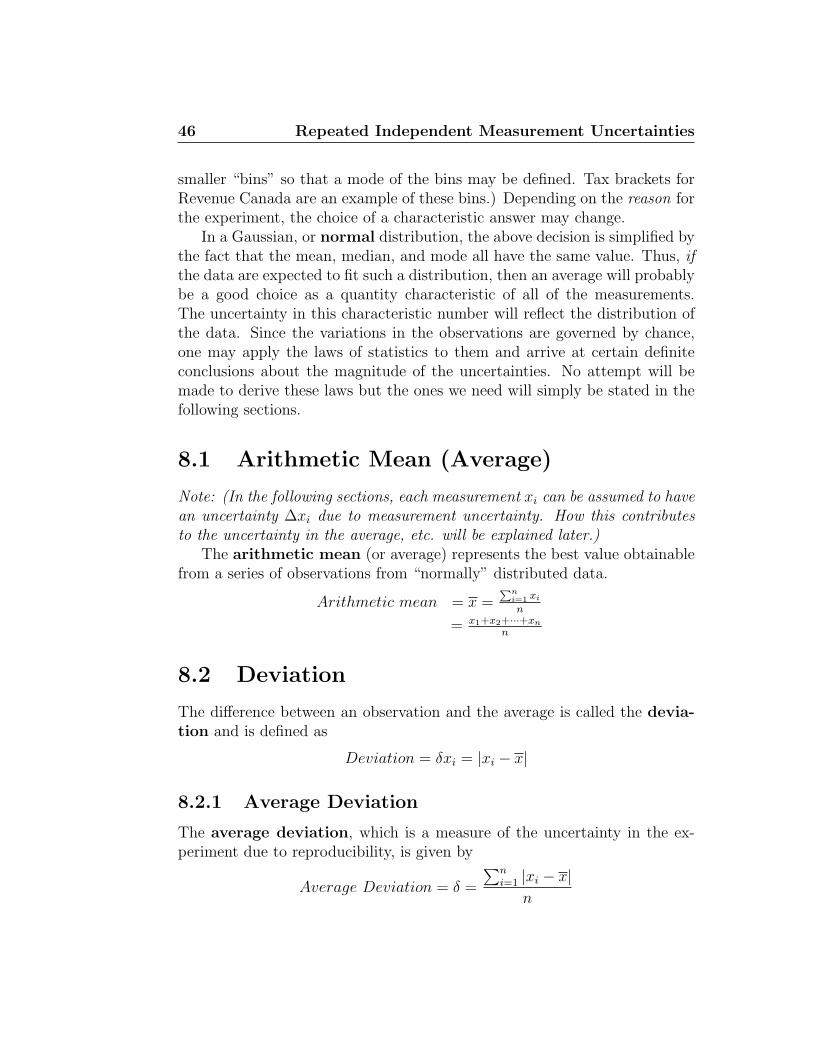
46 Repeated Independent Measurement Uncertainties

smaller “bins” so that a mode of the bins may be defined. Tax brackets forRevenue Canada are an example of these bins.) Depending on the reason forthe experiment, the choice of a characteristic answer may change.

In a Gaussian, or normal distribution, the above decision is simplified bythe fact that the mean, median, and mode all have the same value. Thus, ifthe data are expected to fit such a distribution, then an average will probablybe a good choice as a quantity characteristic of all of the measurements.The uncertainty in this characteristic number will reflect the distribution ofthe data. Since the variations in the observations are governed by chance,one may apply the laws of statistics to them and arrive at certain definiteconclusions about the magnitude of the uncertainties. No attempt will bemade to derive these laws but the ones we need will simply be stated in thefollowing sections.

8.1 Arithmetic Mean (Average)

Note: (In the following sections, each measurement xi can be assumed to havean uncertainty ∆xi due to measurement uncertainty. How this contributesto the uncertainty in the average, etc. will be explained later.)

The arithmetic mean (or average) represents the best value obtainablefrom a series of observations from “normally” distributed data.

Arithmetic mean = x =Pn

i=1 xi

n

= x1+x2+···+xn

n

8.2 Deviation

The difference between an observation and the average is called the devia-tion and is defined as

Deviation = δxi = |xi − x|

8.2.1 Average Deviation

The average deviation, which is a measure of the uncertainty in the ex-periment due to reproducibility, is given by

Average Deviation = δ =

∑ni=1 |xi − x|

n

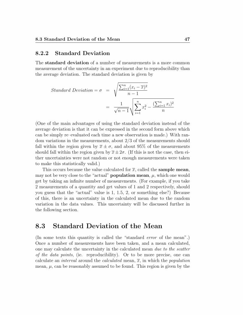
8.3 Standard Deviation of the Mean 47

8.2.2 Standard Deviation

The standard deviation of a number of measurements is a more commonmeasurement of the uncertainty in an experiment due to reproducibility thanthe average deviation. The standard deviation is given by

Standard Deviation = σ =

√∑ni=1(xi − x)2

n− 1

=1√

n− 1

√√√√ n∑i=1

x2i −

(∑n

i=1 xi)2

n

(One of the main advantages of using the standard deviation instead of theaverage deviation is that it can be expressed in the second form above whichcan be simply re–evaluated each time a new observation is made.) With ran-dom variations in the measurements, about 2/3 of the measurements shouldfall within the region given by x ± σ, and about 95% of the measurementsshould fall within the region given by x±2σ. (If this is not the case, then ei-ther uncertainties were not random or not enough measurements were takento make this statistically valid.)

This occurs because the value calculated for x, called the sample mean,may not be very close to the “actual” population mean, µ, which one wouldget by taking an infinite number of measurements. (For example, if you take2 measurements of a quantity and get values of 1 and 2 respectively, shouldyou guess that the “actual” value is 1, 1.5, 2, or something else?) Becauseof this, there is an uncertainty in the calculated mean due to the randomvariation in the data values. This uncertainty will be discussed further inthe following section.

8.3 Standard Deviation of the Mean

(In some texts this quantity is called the “standard error of the mean”.)Once a number of measurements have been taken, and a mean calculated,one may calculate the uncertainty in the calculated mean due to the scatterof the data points, (ie. reproducibility). Or to be more precise, one cancalculate an interval around the calculated mean, x, in which the populationmean, µ, can be reasonably assumed to be found. This region is given by the

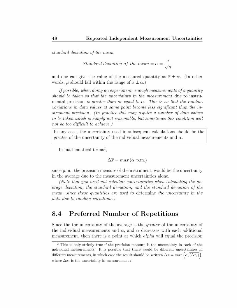
48 Repeated Independent Measurement Uncertainties

standard deviation of the mean,

Standard deviation of the mean = α =σ√n

and one can give the value of the measured quantity as x ± α. (In otherwords, µ should fall within the range of x± α.)

If possible, when doing an experiment, enough measurements of a quantityshould be taken so that the uncertainty in the measurement due to instru-mental precision is greater than or equal to α. This is so that the randomvariations in data values at some point become less significant than the in-strument precision. (In practice this may require a number of data valuesto be taken which is simply not reasonable, but sometimes this condition willnot be too difficult to achieve.)

In any case, the uncertainty used in subsequent calculations should be thegreater of the uncertainty of the individual measurements and α.

In mathematical terms2,

∆x = max (α, p.m.)

since p.m., the precision measure of the instrument, would be the uncertaintyin the average due to the measurement uncertainties alone.

(Note that you need not calculate uncertainties when calculating the av-erage deviation, the standard deviation, and the standard deviation of themean, since these quantities are used to determine the uncertainty in thedata due to random variations.)

8.4 Preferred Number of Repetitions

Since the the uncertainty of the average is the greater of the uncertainty ofthe individual measurements and α, and α decreases with each additionalmeasurement, then there is a point at which alpha will equal the precision

2 This is only strictly true if the precision measure is the uncertainty in each of theindividual measurements. It is possible that there would be different uncertainties indifferent measurements, in which case the result should be written ∆x = max

(α, (∆xi)

),

where ∆xi is the uncertainty in measurement i.

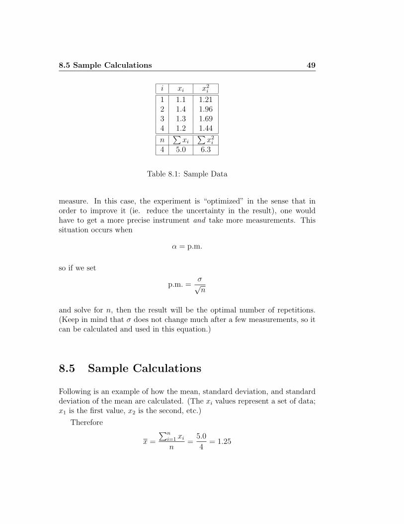
8.5 Sample Calculations 49

i xi x2i

1 1.1 1.212 1.4 1.963 1.3 1.694 1.2 1.44

n∑

xi

∑x2

i

4 5.0 6.3

Table 8.1: Sample Data

measure. In this case, the experiment is “optimized” in the sense that inorder to improve it (ie. reduce the uncertainty in the result), one wouldhave to get a more precise instrument and take more measurements. Thissituation occurs when

α = p.m.

so if we set

p.m. =σ√n

and solve for n, then the result will be the optimal number of repetitions.(Keep in mind that σ does not change much after a few measurements, so itcan be calculated and used in this equation.)

8.5 Sample Calculations

Following is an example of how the mean, standard deviation, and standarddeviation of the mean are calculated. (The xi values represent a set of data;x1 is the first value, x2 is the second, etc.)

Therefore

x =

∑ni=1 xi

n=

5.0

4= 1.25

50 Repeated Independent Measurement Uncertainties

and so

σ =

√∑ni=1(xi − x)2

n− 1

=1√

n− 1

√√√√ n∑i=1

x2i −

(∑n

i=1 xi)2

n

=1√

4− 1

√(6.3)− (5.0)2

4= 0.129099

thus

α =σ√n

=0.129099√

4= 0.06455

The uncertainty which should be quoted with the average above will bethe bigger of the uncertainties in the individual measurements and the stan-dard deviation of the mean. So, if the above xi values all had an uncertaintyof 0.05, then since 0.05 is less than α, we would write

x = 1.25± 0.06

If, on the other hand, the xi had an uncertainty of 0.07 units, then we wouldwrite

x = 1.25± 0.07

since 0.07 is greater than α.Note that in both of these cases, the uncertainties have been rounded to

one significant digit, and the average is rounded so that its last significantdigit is the uncertain one, as required.

8.6 Simple Method; The Method of Quartiles

There is a way to get values very close to those given by calculating themean and standard deviation of the mean with very little calculation. (Thiswill be true if the data have a Gaussian3 distribution.) The method involvesdividing the data into quartiles. The first quartile is the value which is above

3or “normal”

8.6 Simple Method; The Method of Quartiles 51

1/4 of the data values; the second quartile is the value which is above 1/2of the data values4 and so on. The second quartile gives a good estimatefor the average, and the third quartile minus the first quartile gives a goodestimate5 for the standard deviation. Thus,

x± α ≈ Q2 ±(Q3 −Q1)√

n

If you use a number of data values which is a perfect square, such as 16, thenthe only calculation is one division!

4which is also the median5Actually the inter-quartile distance or IQR ≈ 1.35 σ for normally distributed data.

52 Repeated Independent Measurement Uncertainties

Chapter 9

Repeated DependentMeasurements: ConstantIntervals

9.1 The Method of Differences

Occasionally, one performs an experiment which produces more data than isabsolutely necessary. (This is especially true when using electronic equipmentwhich automates data collection.) For example, when doing an experimentmeasuring the position of a cart on a track at fixed time intervals you mayproduce several data points as shown in Figure 9.1.

Consider the situation in Figure 9.1. The first 3 cases all have 6 dotsspaced 1 second apart, for a total time interval of 5 seconds. The fourthcase has only two dots, but they are spaced 5 seconds apart, so again thetotal time interval is 5 seconds. If we were to calculate the velocity usingendpoints alone, all four sets of data would give the same answer. Theimportant question for us is “Which data set do you trust the most?”, or inmore scientific terms, “Which data set has the smallest uncertainty?”

1. Consider cases 1 and 2. The centres of the corresponding dots are atexactly the same times, so each sub-interval is identical. However, thedots in case 1 are much larger. Because of the dot size, we would preferthe data in case 2, or in other words, case 2 has the smaller uncertaintydue to the smaller dots.

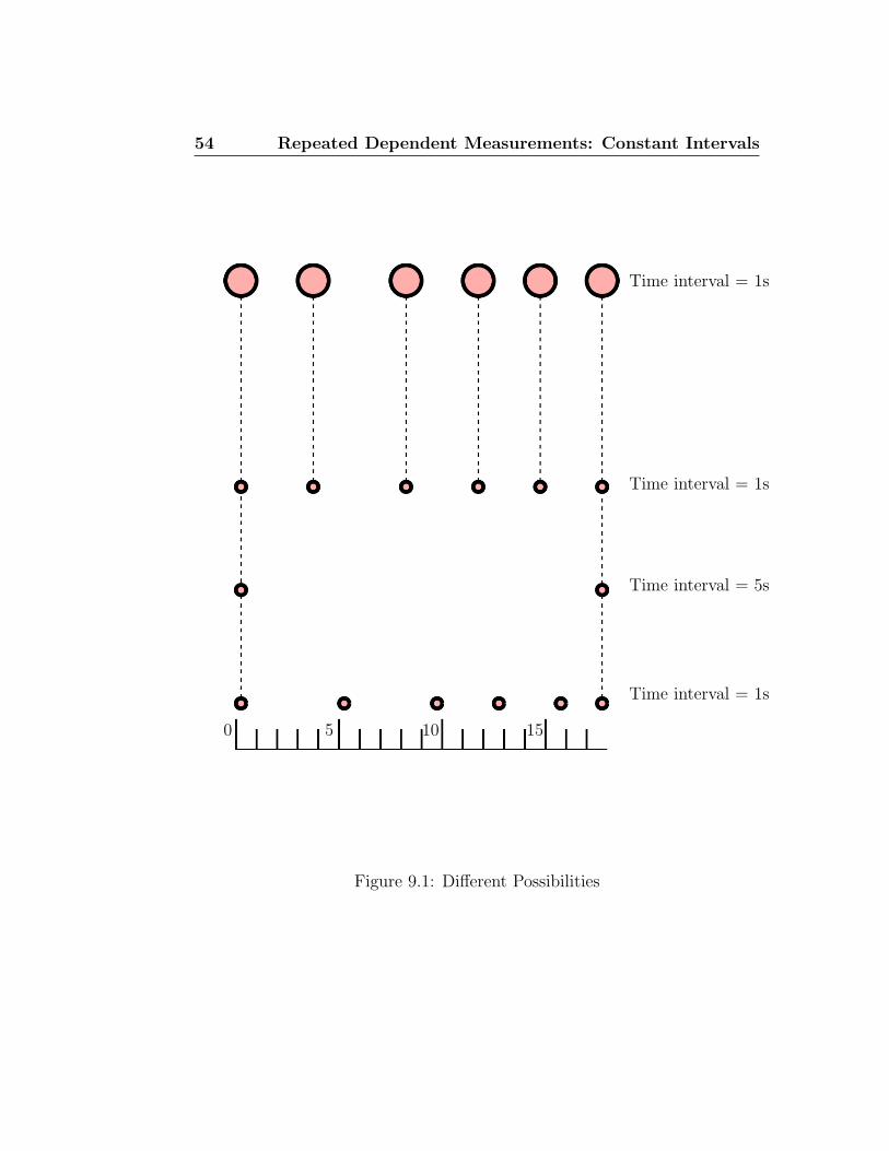
54 Repeated Dependent Measurements: Constant Intervals

Time interval = 1s

Time interval = 1s

Time interval = 5s

Time interval = 1s

0 5 10 15

Figure 9.1: Different Possibilities

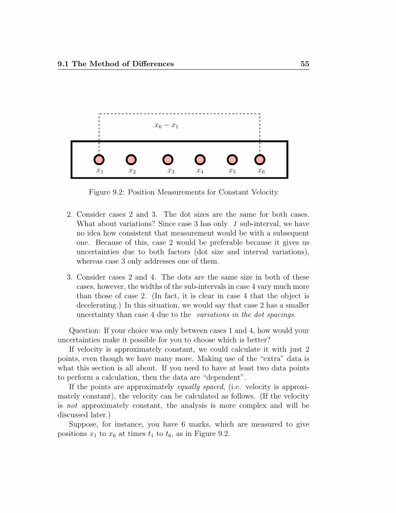
9.1 The Method of Differences 55

x1 x2 x3 x4 x5 x6

x6 − x1

Figure 9.2: Position Measurements for Constant Velocity

2. Consider cases 2 and 3. The dot sizes are the same for both cases.What about variations? Since case 3 has only 1 sub-interval, we haveno idea how consistent that measurement would be with a subsequentone. Because of this, case 2 would be preferable because it gives usuncertainties due to both factors (dot size and interval variations),whereas case 3 only addresses one of them.

3. Consider cases 2 and 4. The dots are the same size in both of thesecases, however, the widths of the sub-intervals in case 4 vary much morethan those of case 2. (In fact, it is clear in case 4 that the object isdecelerating.) In this situation, we would say that case 2 has a smalleruncertainty than case 4 due to the variations in the dot spacings.

Question: If your choice was only between cases 1 and 4, how would youruncertainties make it possible for you to choose which is better?

If velocity is approximately constant, we could calculate it with just 2points, even though we have many more. Making use of the “extra” data iswhat this section is all about. If you need to have at least two data pointsto perform a calculation, then the data are “dependent”.

If the points are approximately equally spaced, (i.e. velocity is approxi-mately constant), the velocity can be calculated as follows. (If the velocityis not approximately constant, the analysis is more complex and will bediscussed later.)

Suppose, for instance, you have 6 marks, which are measured to givepositions x1 to x6 at times t1 to t6, as in Figure 9.2.

56 Repeated Dependent Measurements: Constant Intervals

9.1.1 Option I: End Points

The simplest way we can calculate v is to use just two points. Clearly, theuncertainty in v will be minimized if we use points that are as far apart aspossible to calculate the interval width; i.e.

v =x6 − x1

t6 − t1(9.1)

The uncertainty in the result due to the precision measure of the measuringinstrument can be calculated as usual. Now, is there any way we can use allof the data to produce better results?

9.1.2 Option II (Better):Method of Differences

While the data can be considered as 1 interval of width 5, we can use thepoints we ignored and see the data as 3 independent intervals of width 3, asin Figure 9.3.

Suppose we calculate x as

width1 = x6 − x3 (9.2)

width2 = x5 − x2 (9.3)

width3 = x4 − x1 (9.4)

and then

x =width1 + width2 + width3

3(9.5)

(the average of the 3 widths) and similar for t. The velocity will be given by

v =x

t(9.6)

In this way, we turn 1 interval of 5 into 3 independent intervals of 3! Nowthese 3 independent measurements can be treated as usual, with standarddeviations, etc. The value in this is that now all of the data are used, andvariations in the interval spacing will affect the uncertainty by increasing thestandard deviation of the mean. (Note each measurement is used once andonly once, so all have equal weight.)

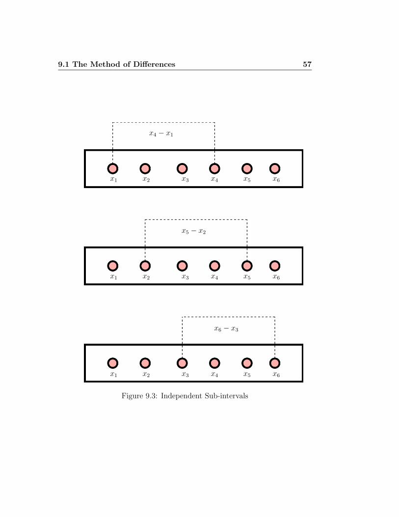
9.1 The Method of Differences 57

x1 x2 x3 x4 x5 x6

x6 − x3

x1 x2 x3 x4 x5 x6

x5 − x2

x1 x2 x3 x4 x5 x6

x4 − x1

Figure 9.3: Independent Sub-intervals

58 Repeated Dependent Measurements: Constant Intervals

The uncertainty in your result will be the bigger of the uncertainty from theprecision measure and the standard deviation of the mean.(In this example,the uncertainty due to the precision measure would be 2∆x. If this is unclear,ask.)

Whenever you have data like this, you should use this method.

9.1.3 Non-Option III :Average All of the Sub-Intervals

You may be wondering why we don’t average all of the sub-intervals; in otherwords, why not determine

v =xi+1 − xi

ti+1 − ti(9.7)

for i = 1, 2, . . . 6. If you expand this out, you get

v =x6−x5

t6−t5+ x5−x4

t5−t4· · · x3−x2

t3−t2+ x2−x1

t2−t1

5(9.8)

Since all of the time intervals are the same, this becomes

v =(x6 − x5) + (x5 − x4) · · · (x3 − x2) + (x2 − x1)

5∆t(9.9)

Removing the brackets gives

v =x6 −��x5 +��x5 −ZZx4 · · ·ZZx3 −��x2 +��x2 − x1

5∆t(9.10)

Notice we have both a ‘+’ and a ‘-’ term for each of x2 to x5, so that we areleft with

v =x6 − x1

5∆t(9.11)

which is exactly what we get by using the endpoints alone! This is why, withequal time intervals1, there is no point to averaging all of the intervals.

1Note that if the time intervals are not the same, then the simplification from Equa-tion 9.8 to Equation 9.9 cannot happen, so the intermediate points do not automaticallydisappear.

Chapter 10

Uncertain Results

10.1 The most important part of a lab

The “Discussion of Errors” (or Uncertainties) section of a lab report is whereyou outline the reasonable limits which you place on your results. If you havedone a professional job of your research, you should be prepared to defendyour results. In other words, you should expect anyone else to get resultswhich agree with yours; if not, you suspect theirs. In this context, you wantto discuss sources of error which you have reason to believe are significant.

10.1.1 Operations with Uncertainties

When numbers, some or all of which are approximate, are combined by ad-dition, subtraction, multiplication, or division, the uncertainty in the resultsdue to the uncertainties in the data is given by the range of possible calculatedvalues based on the range of possible data values.

Remember: Since uncertainties are an indication of the imprecise nature of aquantity, uncertainties are usually only expressed to one decimal place. (Inother words, it doesn’t make sense to have an extremely precise measure ofthe imprecision in a value!)

For instance, if we have two numbers with uncertainties, such as x = 2±1and y = 32.0 + 0.2, then what that means is that x can be as small as 1 oras big as 3, while y can be as small as 31.8 or as big as 32.2 so adding themcan give a result x+y which can be as small as 32.8 or as big as 35.2, so that

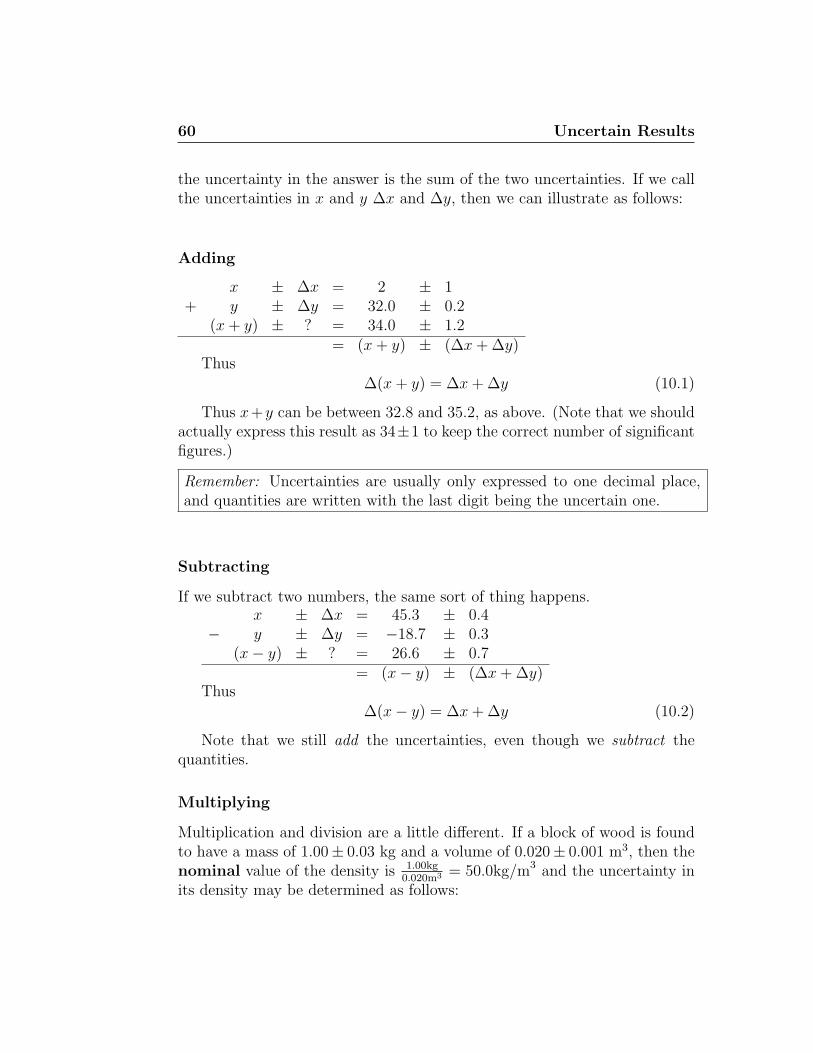
60 Uncertain Results

the uncertainty in the answer is the sum of the two uncertainties. If we callthe uncertainties in x and y ∆x and ∆y, then we can illustrate as follows:

Adding

x ± ∆x = 2 ± 1+ y ± ∆y = 32.0 ± 0.2

(x + y) ± ? = 34.0 ± 1.2= (x + y) ± (∆x + ∆y)

Thus

∆(x + y) = ∆x + ∆y (10.1)

Thus x+y can be between 32.8 and 35.2, as above. (Note that we shouldactually express this result as 34±1 to keep the correct number of significantfigures.)

Remember: Uncertainties are usually only expressed to one decimal place,and quantities are written with the last digit being the uncertain one.

Subtracting

If we subtract two numbers, the same sort of thing happens.x ± ∆x = 45.3 ± 0.4

− y ± ∆y = −18.7 ± 0.3(x− y) ± ? = 26.6 ± 0.7

= (x− y) ± (∆x + ∆y)Thus

∆(x− y) = ∆x + ∆y (10.2)

Note that we still add the uncertainties, even though we subtract thequantities.

Multiplying

Multiplication and division are a little different. If a block of wood is foundto have a mass of 1.00± 0.03 kg and a volume of 0.020± 0.001 m3, then thenominal value of the density is 1.00kg

0.020m3 = 50.0kg/m3 and the uncertainty inits density may be determined as follows:

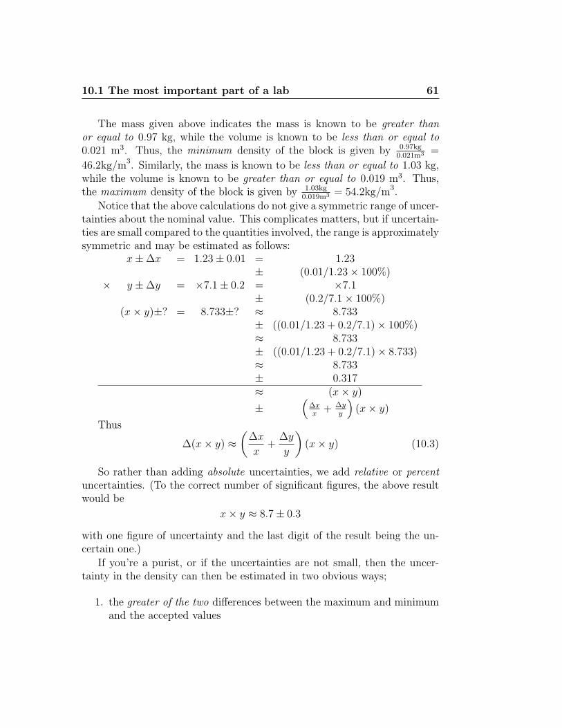
10.1 The most important part of a lab 61

The mass given above indicates the mass is known to be greater thanor equal to 0.97 kg, while the volume is known to be less than or equal to0.021 m3. Thus, the minimum density of the block is given by 0.97kg

0.021m3 =

46.2kg/m3. Similarly, the mass is known to be less than or equal to 1.03 kg,while the volume is known to be greater than or equal to 0.019 m3. Thus,the maximum density of the block is given by 1.03kg

0.019m3 = 54.2kg/m3.

Notice that the above calculations do not give a symmetric range of uncer-tainties about the nominal value. This complicates matters, but if uncertain-ties are small compared to the quantities involved, the range is approximatelysymmetric and may be estimated as follows:

x±∆x = 1.23± 0.01 = 1.23± (0.01/1.23× 100%)

× y ±∆y = ×7.1± 0.2 = ×7.1± (0.2/7.1× 100%)

(x× y)±? = 8.733±? ≈ 8.733± ((0.01/1.23 + 0.2/7.1)× 100%)≈ 8.733± ((0.01/1.23 + 0.2/7.1)× 8.733)≈ 8.733± 0.317≈ (x× y)

±(

∆xx

+ ∆yy

)(x× y)

Thus

∆(x× y) ≈(

∆x

x+

∆y

y

)(x× y) (10.3)

So rather than adding absolute uncertainties, we add relative or percentuncertainties. (To the correct number of significant figures, the above resultwould be

x× y ≈ 8.7± 0.3

with one figure of uncertainty and the last digit of the result being the un-certain one.)

If you’re a purist, or if the uncertainties are not small, then the uncer-tainty in the density can then be estimated in two obvious ways;

1. the greater of the two differences between the maximum and minimumand the accepted values

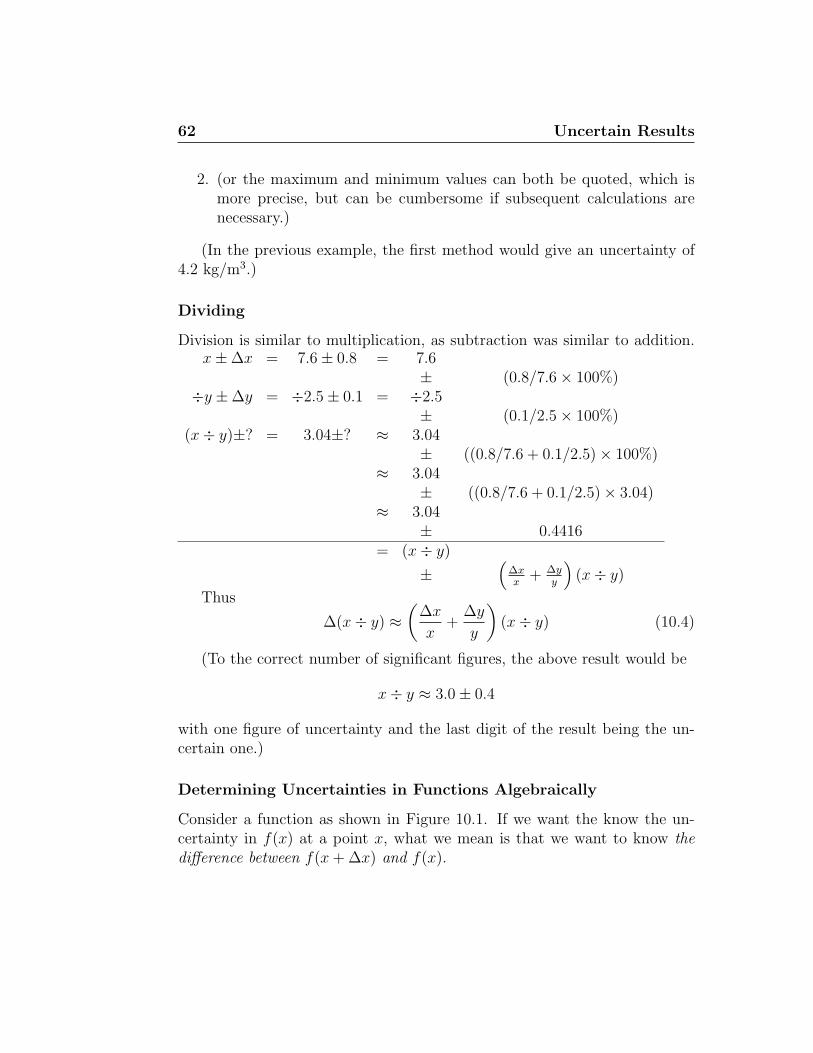
62 Uncertain Results

2. (or the maximum and minimum values can both be quoted, which ismore precise, but can be cumbersome if subsequent calculations arenecessary.)

(In the previous example, the first method would give an uncertainty of4.2 kg/m3.)

Dividing

Division is similar to multiplication, as subtraction was similar to addition.x±∆x = 7.6± 0.8 = 7.6

± (0.8/7.6× 100%)÷y ±∆y = ÷2.5± 0.1 = ÷2.5

± (0.1/2.5× 100%)(x÷ y)±? = 3.04±? ≈ 3.04

± ((0.8/7.6 + 0.1/2.5)× 100%)≈ 3.04

± ((0.8/7.6 + 0.1/2.5)× 3.04)≈ 3.04

± 0.4416= (x÷ y)

±(

∆xx

+ ∆yy

)(x÷ y)

Thus

∆(x÷ y) ≈(

∆x

x+

∆y

y

)(x÷ y) (10.4)

(To the correct number of significant figures, the above result would be

x÷ y ≈ 3.0± 0.4

with one figure of uncertainty and the last digit of the result being the un-certain one.)

Determining Uncertainties in Functions Algebraically

Consider a function as shown in Figure 10.1. If we want the know the un-certainty in f(x) at a point x, what we mean is that we want to know thedifference between f(x + ∆x) and f(x).

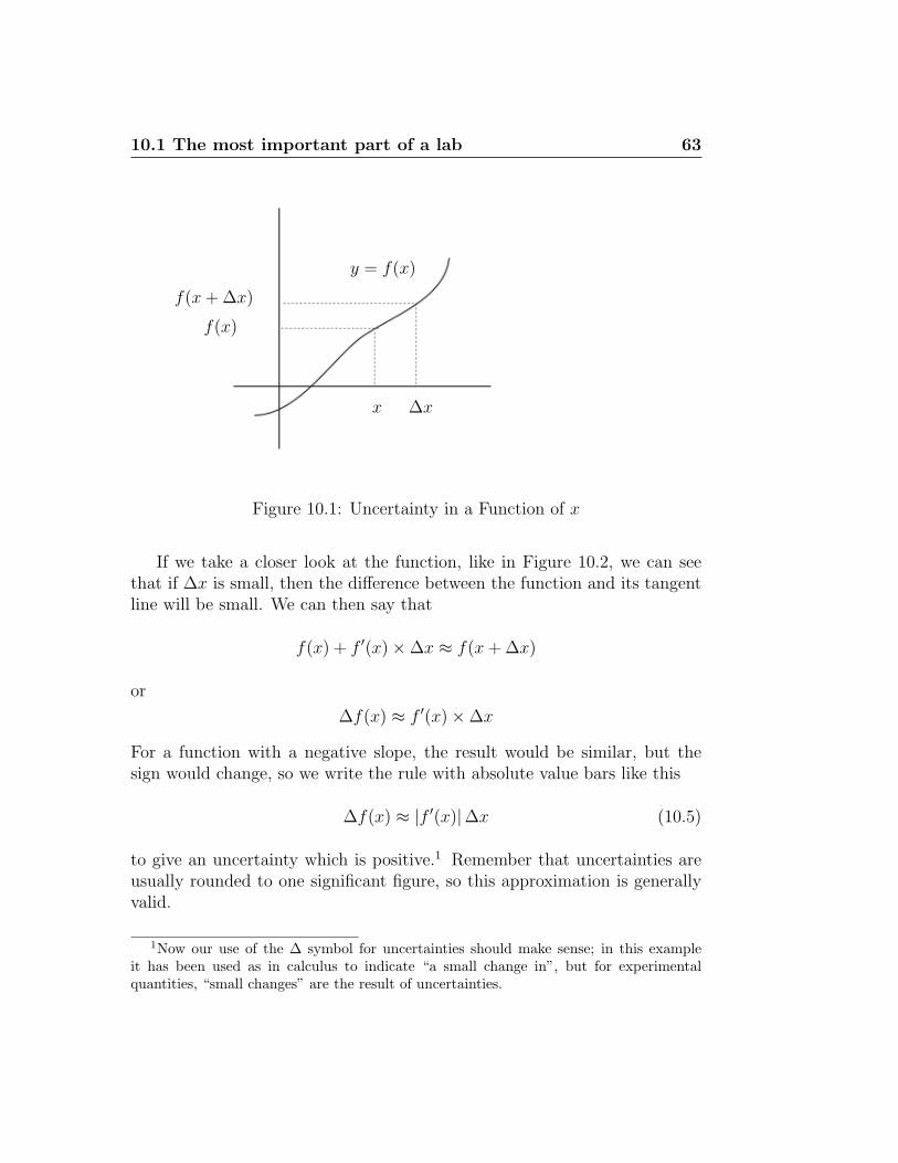
10.1 The most important part of a lab 63

f(x)

y = f(x)

x

f(x + ∆x)

∆x

Figure 10.1: Uncertainty in a Function of x

If we take a closer look at the function, like in Figure 10.2, we can seethat if ∆x is small, then the difference between the function and its tangentline will be small. We can then say that

f(x) + f ′(x)×∆x ≈ f(x + ∆x)

or

∆f(x) ≈ f ′(x)×∆x

For a function with a negative slope, the result would be similar, but thesign would change, so we write the rule with absolute value bars like this

∆f(x) ≈ |f ′(x)|∆x (10.5)

to give an uncertainty which is positive.1 Remember that uncertainties areusually rounded to one significant figure, so this approximation is generallyvalid.

1Now our use of the ∆ symbol for uncertainties should make sense; in this exampleit has been used as in calculus to indicate “a small change in”, but for experimentalquantities, “small changes” are the result of uncertainties.

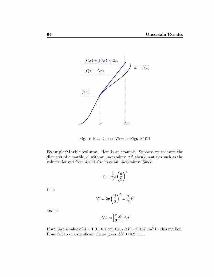
64 Uncertain Results

y = f(x)

f(x)

x

f(x + ∆x)

f(x) + f ′(x)×∆x

∆x

Figure 10.2: Closer View of Figure 10.1

Example:Marble volume Here is an example. Suppose we measure thediameter of a marble, d, with an uncertainty ∆d, then quantities such as thevolume derived from d will also have an uncertainty. Since

V =4

3π

(d

2

)3

then

V ′ = 2π

(d

2

)2

=π

2d2

and so

∆V ≈∣∣∣π2d2∣∣∣∆d

If we have a value of d = 1.0±0.1 cm, then ∆V = 0.157 cm3 by this method.Rounded to one significant figure gives ∆V ≈ 0.2 cm3.

10.1 The most important part of a lab 65

Determining Uncertainties in Functions by Inspection

Note: In the following section and elsewhere in the manual, the notation ∆xis used to mean “the uncertainty in x”.

When we have a measurement of 2.0± 0.3 cm, this means that the max-imum value it can have is 2.0 + 0.3cm. The uncertainty is the differencebetween this maximum value and the nominal value (ie. the one with nouncertainty). We could also say that the minimum value it can have is2.0−0.3 cm, and the uncertainty is the difference between the nominal valueand this maximum value. Thus if we want to find the uncertainty in a func-tion, f(x), we can say that

∆f(x) ≈ fmax − f (10.6)

or∆f(x) ≈ f − fmin (10.7)

where fmax is the same function with x replaced by either x+∆x or x−∆x;whichever makes f bigger, and fmin is the same function with x replaced byeither x + ∆x or x − ∆x; whichever makes f smaller. (The approximatelyequals sign is to reflect the fact that these two values may not be quite thesame, depending on the function f .) For instance, if

f(x) = x2 + 5

then clearly, if x is positive, then replacing x by x + ∆x will make f amaximum.

fmax = f(x + ∆x) = (x + ∆x)2 + 5

and so

∆f(x) ≈ fmax − f = f(x + ∆x)− f(x) =((x + ∆x)2 + 5

)−(x2 + 5

)On the other hand, if we wanted to find the uncertainty in

g(t) =1√t

then, if t is positive, then replacing t by t−∆t will make g a maximum.

gmax = g(t−∆t) =1√

(t−∆t)

66 Uncertain Results

and so

∆g(t) ≈ gmax − g = g(t−∆t)− g(t) =

(1√

(t−∆t)

)−(

1√t

)If we had a function of two variables,

h(w, z) =

√w

z2

then we want to replace each quantity with the appropriate value in orderto maximize the total, so if w and z are both positive,

hmax =

√(w + ∆w)

(z −∆z)2

and thus

∆h ≈ hmax − h =

√(w + ∆w)

(z −∆z)2 −√

w

z2

Notice in each of these cases, it was necessary to restrict the range of thevariable in order to determine whether the uncertainty should be added orsubtracted in order to maximize the result. In an experiment, usually yourdata will automatically be restricted in certain ways. (For instance, massesare always positive.)

Example:Marble volume Using the above example of the volume of amarble,

∆V ≈ V (d + ∆d)− V (d)

Since

V =4

3π

(d

2

)3

then

∆V ≈ 4

3π

(d + ∆d

2

)3

− 4

3π

(d

2

)3

If we have a value of d = 1.0±0.1 cm, then ∆V = 0.173 cm3 by this method.Rounded to one significant figure gives ∆V ≈ 0.2 cm3 as the value to bequoted.

10.1 The most important part of a lab 67

Determining Uncertainties by Trial and Error

For a function f(x, y), the uncertainty in f will be given by the biggest of

|f(x + ∆x, y + ∆y)− f(x, y)|

or

|f(x−∆x, y + ∆y)− f(x, y)|

or

|f(x + ∆x, y −∆y)− f(x, y)|

or

|f(x−∆x, y −∆y)− f(x, y)|

Note that for each variable with an uncertainty, the number of possibilitiesdoubles. In most cases, common sense will tell you which one is going to bethe important one, but things like the sign of numbers involved, etc. willmatter a lot! For example, if you are adding two positive quantities, thenthe first or fourth above will give the same (correct) answer. However, if onequantity is negative, then the second and third will be correct.

The advantage of knowing this method is that it always works. Sometimesit may be easier to go through this approach than to do all of the algebraneeded for a complicated expression, especially if common sense makes iteasy to see which combination of signs gives the correct answer.

Determining Uncertainties Algebraically

To summarize, the uncertainty in results can usually be calculated as in thefollowing examples (if the percentage uncertainties in the data are small):

(a) ∆(A + B) = (∆A + ∆B)

(b) ∆(A−B) = (∆A + ∆B)

(c) ∆(A×B) ≈ |AB|(∣∣∆A

A

∣∣+ ∣∣∆BB

∣∣)(d) ∆(A

B) ≈

∣∣AB

∣∣ (∣∣∆AA

∣∣+ ∣∣∆BB

∣∣)(e) ∆f(A±∆A) ≈ |f ′(A)|∆A

Note that the first two rules above always hold true.

68 Uncertain Results

To put it another way, when adding or subtracting, you add absolute un-certainties. When multiplying or dividing, you add percent or relative uncer-tainties. Note that for the last rule above that angles and their uncertaintiesmust be in radians for the differentiation to be correct! (In the examplesabove, absolute value signs were omitted since all positive quantities wereused.) (Some specific uncertainty results can be found in Appendix I.)

Remember that a quantity and its uncertainty should always have the sameunits, so you can check units when calculating uncertainties to avoid mis-takes.

Example: Marble volume If we have a value of d = 1.0 ± 0.1 cm, asused previously, then ∆V = 0.157 cm3 by this method.

Mathematically, this result and the previous one are equal if ∆d << d. Youcan derive this using the binomial approximation, which simply meansmultiplying it out and discarding and terms with two or more ∆ terms mul-tiplied together; for instance ∆A∆B ≈ 0

Choosing Algebra or Inspection

Since uncertainties are usually only expressed to one decimal place, thensmall differences given by different methods of calculation, (ie. inspection oralgebra), do not matter.

Example: Marble volume Using the previous example of the marble, ifwe have a value of d = 1.0± 0.1 cm, then ∆V = 0.173 cm3 by the inspectionmethod. Rounded to one significant figure gives ∆V ≈ 0.2 cm3 as the valueto be quoted. By the algebraic method, ∆V = 0.157 cm3. Rounded to onesignificant figure gives ∆V ≈ 0.2 cm3, which is the same as that given by theprevious method. So in this example a 10% uncertainty in d was still smallenough to give the same result (to one significant figure) by both methods.

Sensitivity of Total Uncertainty to Individual Uncertainties

When you discuss sources of uncertainty in an experiment, it is important torecognize which ones contributed most to the uncertainty in the final result.

10.1 The most important part of a lab 69

In order to determine this, proceed as follows:

1. Write out the equation for the uncertainty in the result, using whichevermethod you prefer.

2. For each of the quantities in the equation which have an uncertainty,calculate the uncertainty in the result which you get if all of the otheruncertainties are zero.

3. Arrange the quantities in descending order based on the size of theuncertainties calculated. The higher in the list a quantity is, the greaterit’s contribution to the total uncertainty.

The sizes of these uncertainties should tell you which factors need to beconsidered, remembering that only quantities contributing 10% or more tothe total uncertainty matter. For example, from before we had a function of

two variables,

h(w, z) =

√w

z2

so by inspection, its uncertainty is given by

∆h ≈ hmax − h =

√(w + ∆w)

(z −∆z)2 −√

w

z2

So we can compute

∆hw ≈√

(w + ∆w)

z2−√

w

z2

and

∆hz ≈√

w

(z −∆z)2 −√

w

z2

Note that in the first equation, all of the ∆z terms are gone, and in thesecond, all of the ∆w terms are gone. By the algebraic method,

∆h ≈√

w

z2

(∆w

2w+

2∆z

z

)and so

∆hw ≈√

w

z2

(∆w

2w

)

70 Uncertain Results

and

∆hz ≈√

w

z2

(2∆z

z

)Note that until you plug values into these equations, you can’t tell whichuncertainty contribution is larger.

In the above example, if we use values of w = 1.00 ± 0.01 and z =2.00±0.02, then the proportional uncertainties in both w and z are the same,1%. However, using either inspection or the algebraic method, ∆h = 0.006,and ∆hw = 0.001 while ∆hz = 0.005; in other words, the uncertainty in theresult due to ∆z is five times the uncertainty due to ∆w! (As you get moreused to uncertainty calculations, you should realize this is because z is raisedto a higher power than w, and so its uncertainty counts for more.) In orderto improve this experiment, it would be more important to try and reduce∆z than it would be to try and reduce ∆w.

Simplifying Uncertainties

Uncertainty calculations can get quite involved if there are several quantitiesinvolved. However, since uncertainties are usually only carried to one ortwo significant figures at most, there is little value in carrying uncertaintiesthrough calculations if they do not contribute significantly to the total.

You do not need to carry uncertainties through if they do not contributemore than 10% of the total uncertainty, since uncertainties are usually onlyexpressed to one decimal place. (However, be sure to give bounds for theseuncertainties when you do this.)

Note that this shows a difference between doing calculations by handversus using a spreadsheet. If you are doing calculations by hand, it makessense to drop insignificant uncertainties like this.

If you’re using a spreadsheet in order to allow you to change the data andrecalculate, it may be worth carrying all uncertainties through in case someof them may be more significant for different data.

10.1 The most important part of a lab 71

10.1.2 Uncertainties and Final Results

When an experiment is performed, it is crucial to determine whether or notthe results make sense. In other words, do any calculated quantities fallwithin a “reasonable” range?

The reason for doing calculations with uncertainties is so that uncertain-ties in final answers can be obtained. If, for instance, a physical constantwas measured, the calculated uncertainty determines the range around thecalculated value in which one would expect to find the “theoretical” value.If the theoretical value falls within this range, then we say that our resultsagree with the theory within our experimental uncertainty.

For instance, if we perform an experiment and get a value for the accel-eration due to gravity of g = 9.5 ± 0.5m/s2 then we can say that we saythat our values agrees with the accepted value of g = 9.8m/s2 within ourexperimental uncertainty.

If we have two values to compare, such as initial and final momentum todetermine whether momentum was conserved, then we see if the ranges givenby the two uncertainties overlap. In other words, if there is a value or rangeof values common to both, then they agree within experimental uncertainty.

So if an experiment gives us a value of pi = 51.2 ± 0.7 kg-m/s and pf =50.8 ± 0.5 kg-m/s, then we would say the values agree within experimentaluncertainty since the range from 50.5 kg-m/s → 51.3 kg-m/s is common toboth. Since what we were studying was the conservation of momentum, thenwe would say that in this case momentum was conserved within experimentaluncertainty. Note that if both uncertainties were 0.1 kg-m/s, then our resultswould not agree and we would say that momentum was not conserved withinexperimental uncertainty.

Mathematically, if two quantities a and b, with uncertainties ∆a and ∆b arecompared, they can be considered to agree within their uncertainties if

|a− b| ≤ ∆a + ∆b (10.8)

A constant given with no uncertainty given can usually be assumed to havean uncertainty of zero.

If we need to compare 3 or more values this becomes more complex.

If two quantities agree within experimental error, this means that the dis-crepancy between experiment and theory can be readily accounted for on the

72 Uncertain Results

basis of measurement uncertainties which are known. If the theoretical valuedoes not fall within this range, then we say that our results do not agree withthe theory within experimental uncertainty. In this situation, we cannot ac-count for the discrepancy on the basis of measurement uncertainties alone,and so some other factors must be responsible.

If two numbers do not agree within experimental error, then the percentagedifference between the experimental and theoretical values must be calcu-lated as follows:

Percent Difference =

∣∣∣∣theoretical − experimental

theoretical

∣∣∣∣× 100% (10.9)

Remember: Only calculate the percent difference if your results do not agreewithin experimental error.

In our example above, we would not calculate the percentage differencebetween our calculated value for the acceleration due to gravity of g = 9.5±0.5m/s2 and the accepted value of g = 9.8m/s2 since they agree within ourexperimental uncertainty.

Often instead of comparing an experimental value to a theoretical one,we are asked to test a law such as the Conservation of Energy. In this case,what we must do is to compare the initial and final energies of the system inthe manner just outlined.2 If the values agree, then we can say that energywas conserved, and if the values don’t agree then it wasn’t. In that case wewould calculate the percentage difference as follows:

Percent Difference =

∣∣∣∣ initial − final

initial

∣∣∣∣× 100% (10.10)

Significant Figures in Final Results

Always express final answers with absolute uncertainties rather than percentuncertainties. Also, always quote final answers with one significant digit of

2 There is another possibility which you may consider. Suppose you compare the changein energy to its expected value of zero. In that case, any non-zero change would resultin infinite percent difference, which is mathematically correct but not terribly meaningfulphysically.

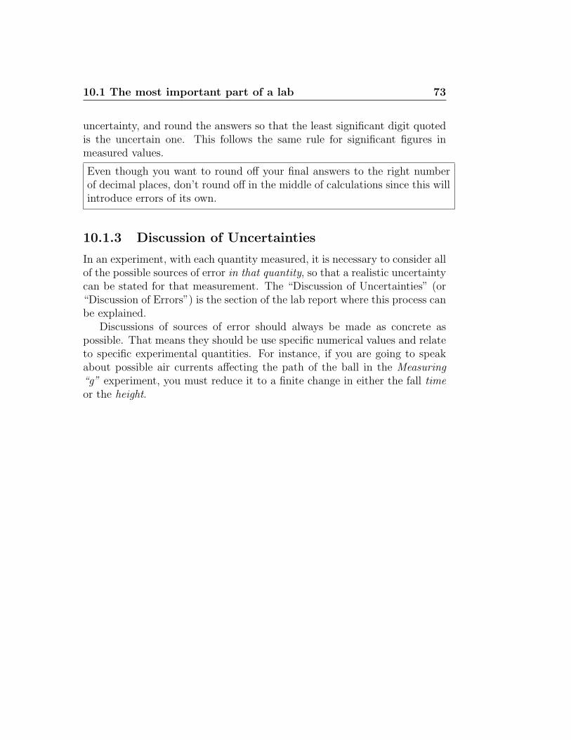
10.1 The most important part of a lab 73

uncertainty, and round the answers so that the least significant digit quotedis the uncertain one. This follows the same rule for significant figures inmeasured values.

Even though you want to round off your final answers to the right numberof decimal places, don’t round off in the middle of calculations since this willintroduce errors of its own.

10.1.3 Discussion of Uncertainties

In an experiment, with each quantity measured, it is necessary to consider allof the possible sources of error in that quantity, so that a realistic uncertaintycan be stated for that measurement. The “Discussion of Uncertainties” (or“Discussion of Errors”) is the section of the lab report where this process canbe explained.

Discussions of sources of error should always be made as concrete aspossible. That means they should be use specific numerical values and relateto specific experimental quantities. For instance, if you are going to speakabout possible air currents affecting the path of the ball in the Measuring“g” experiment, you must reduce it to a finite change in either the fall timeor the height.

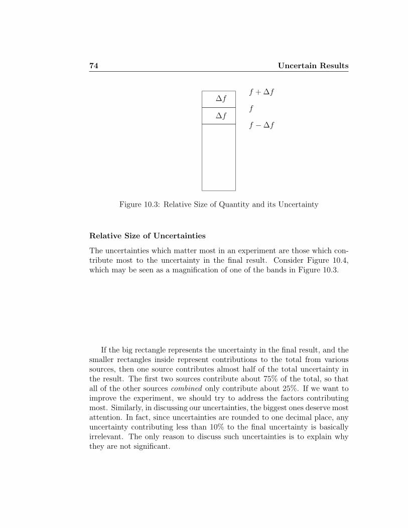
74 Uncertain Results

f −∆f

f

f + ∆f

∆f

∆f

Figure 10.3: Relative Size of Quantity and its Uncertainty

Relative Size of Uncertainties

The uncertainties which matter most in an experiment are those which con-tribute most to the uncertainty in the final result. Consider Figure 10.4,which may be seen as a magnification of one of the bands in Figure 10.3.

If the big rectangle represents the uncertainty in the final result, and thesmaller rectangles inside represent contributions to the total from varioussources, then one source contributes almost half of the total uncertainty inthe result. The first two sources contribute about 75% of the total, so thatall of the other sources combined only contribute about 25%. If we want toimprove the experiment, we should try to address the factors contributingmost. Similarly, in discussing our uncertainties, the biggest ones deserve mostattention. In fact, since uncertainties are rounded to one decimal place, anyuncertainty contributing less than 10% to the final uncertainty is basicallyirrelevant. The only reason to discuss such uncertainties is to explain whythey are not significant.

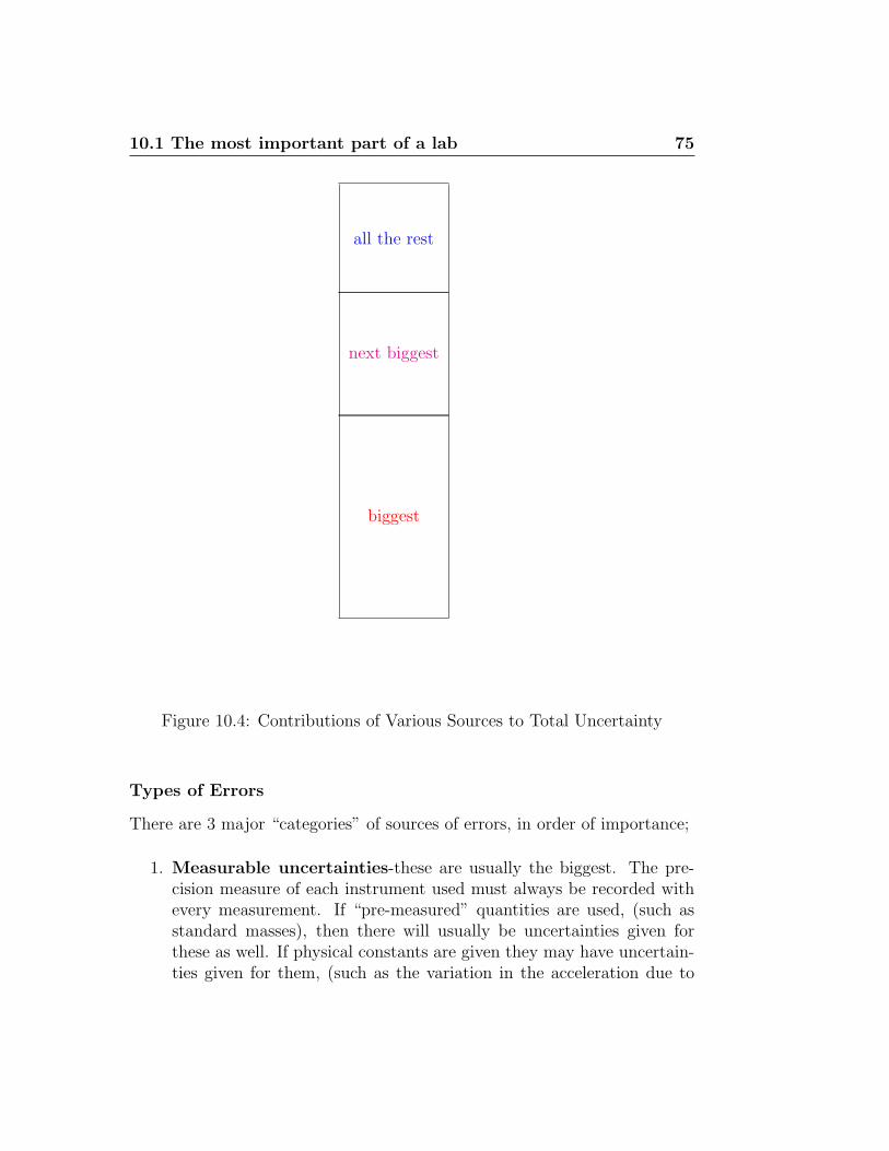
10.1 The most important part of a lab 75

biggest

next biggest

all the rest

Figure 10.4: Contributions of Various Sources to Total Uncertainty

Types of Errors

There are 3 major “categories” of sources of errors, in order of importance;

1. Measurable uncertainties-these are usually the biggest. The pre-cision measure of each instrument used must always be recorded withevery measurement. If “pre-measured” quantities are used, (such asstandard masses), then there will usually be uncertainties given forthese as well. If physical constants are given they may have uncertain-ties given for them, (such as the variation in the acceleration due to

76 Uncertain Results

gravity by height above sea level, latitude, etc.) Where the realisticuncertainty in a quantity comes from any of these, (which will often bethe case), you do not usually need to refer to them in your discussion.However, if there are any which contribute greatly to the uncertainty inyour results, you should discuss them. For example, when you measurethe mass of an object with a balance, then if the precision measure isthe uncertainty used in your calculations, you don’t need to discuss it,unless it is one of the biggest uncertainties in your calculations. Keepin mind that without these values being given, it is impossible to tellwhether any of the following sources of error are significant or not.

2. Bounded uncertainties-these are things which you observed, andhave put limits on and usually are much smaller than those in the groupabove. (Remember that since uncertainties are ultimately rounded toone significant digit, any which contribute less than 10% to the totaluncertainty can be ignored.) Since you have observed them, you cangive some estimate of how much effect they may have. For instance,suppose you measure the length of a table with a metre stick, and no-tice that the ends of the table are not exactly smooth and straight. Ifyou can find a way to measure the variation in the length of the tabledue to this, then you can incorporate this into your uncertainty (if itis big enough) and discuss it.

A plausible error is one which can be tested. If you cannot figure out howto test for an error, it is not worth discussing. (Putting a bound on an errorimplies some method of testing for its existence, even if you are not able todo it at the present time.)

3. Blatant filler-these are things you may be tempted to throw in tosound more impressive. Don’t!!! If you did not observe them, don’t dis-cuss them. If you suggest the gravitational pull of Jupiter is affectingyour results, you’d better be prepared to show evidence (such as get-ting consistently different results at different times of day as the Earthrotates and so changes the angle of Jupiter’s pull.) Do you even knowin which direction the pull of Jupiter would be???

10.1 The most important part of a lab 77

If you are going to discuss a source of uncertainty, then you must either haveincluded it in your calculations, or given some reasonable bounds on its size.If you haven’t done either of those, forget it!

You must discuss at least one source of systematic error in your report, evenif you reject it as insignificant, in order to indicate how it would affect theresults.

Reducing Errors

Whenever errors are discussed, you should suggest how they may be reducedor eliminated. There is a “hierarchy” of improvements which should be ev-ident in your discussion. The following list starts with the best ideas, andprogresses to less useful ones.

1. Be smart in the first place. You should never suggest you may have donesomething wrong in the lab; a professional who recognizes a mistakegoes back and fixes it before producing a report. If you find yourselfmaking a mistake which would seem likely to be repeated by otherpeople, you may want to mention it in your report so that instructionsmay be clarified for the future.

2. Repeat the measurements once or twice to check for consistency. Rep-etition is a very good thing to do if your data are inconsistent or scat-tered. If certain values appear to be incorrect, you may want to repeatthem to make sure. If this seems to be true, and you feel a measurementwas wrong, you should still include it in your report but explain whyit was not used in your calculations. (This is probably similar to theprevious one; if you think your data may be messed up, you should tryto repeat it before you write your report, so this is not something youshould be suggesting in your own report, although you should explainthat you did it if you felt it was necessary.)

3. Change technique. It may be that a different way of doing things,using the same equipment, could (potentially) improve your results. Ifso, this should be explained.

One example of this which may sound odd at first is to try and increasethe error and see what change is produced. For instance, if you neglected

78 Uncertain Results

the mass of something in an experiment, you could increase that massand then repeat the experiment. If the results do not change, then it isunlikely that the original mass had a significant effect.

Question: How big a change in the quantity in question (such as themass just mentioned) should you try? Explain.

4. Make more types of observations. In some cases, monitoring certainthings during the experiment may ensure they do not affect the results.This may be relevant in the case of “bounded uncertainties” above. Itshould be possible with equipment available in the lab. (For instance, ifyou are measuring the speed of sound, and the expected value is givenat 25◦ C, then you might explain a discrepancy by the temperaturebeing different. However, in this case, if you think the temperaturemay have affected your results, then you should check a thermometerto get the actual temperature during the experiment to suggest whetheror not that was likely to have caused an effect.)

5. Repeat the measurements to average the results. While it is alwaysgood to repeat measurements, there is a law of diminishing returns.(In other words, repeating measurements a few times will give you alot of information about how consistent your results are; repeating themmany more times will not tell you as much. That is why the standarddeviation of the mean decreases as 1/

√n, where n is the number of

measurements; as n gets bigger, the change happens more slowly.) Infact, depending on the uncertainties involved, repetition at some pointis of no value. (That is when the standard deviation of the mean getssmaller than the uncertainty in the individual measurements. At thatpoint you cannot improve without using a more precise instrument, nomatter how many times you repeat the experiment.)

6. Change equipment; this is a last resort. Since this in essence meansdoing a different experiment, it is least desirable, and least relevant.Your goal is to produce the best results possible with the equipmentavailable.

Ridiculous Errors

Certain errors crop up from time to time in peoples’ reports without anyjustification. The point of your discussion is to support your results, placing

10.1 The most important part of a lab 79

reasonable bounds on them, not to absolve yourself of responsibility for them.Would you want to hire people who did not have faith in their own research?Including errors merely to “pad” your report is not good; one realistic sourceof error with justification is better than a page full of meaningless ones.Following are some commonly occurring meaningless ones.

• “..human error...”

This is the most irritating statement you can make; you should haveread over the instructions beforehand until you knew what was re-quired, and then performed the experiment to the best of your ability.If you didn’t you were being unprofessional and are wasting the reader’stime. After doing your calculations, you should be able to tell from yourresults if they make sense. If not, you should go back and correct yourerrors. (Note something like reaction time does not fall into this cat-egory, because it is well-defined and can easily be measured. Vague,undefined errors are the big no-no.)

• “..parallax...”

Parallax is the error you get from looking at a scale like a speedometeror a clock from the side; the position of the hands will appear differentdepending on your angle. With just about any scale I’ve seen, I’d behard pressed to get an error of more than 5 → 10% from parallax (andthe latter very rarely). Even that would only occur if I was deliberatelytrying to observe off-axis. Unless there is some reason that you cannoteliminate it, don’t ascribe any significant error to it.

• “..component values may not have been as stated...”

Usually people say this about masses, etc. I’m tempted to say “Well,DUH! ” but I won’t. Of course if given values are incorrect then cal-culations will be in error, but unless you have evidence for a specificvalue being wrong, (which should include some bounds on how wrongit could be), then it is just wild speculation. (You may allow reason-able uncertainties for these given values if you justify them.) Of course,suggesting equipment was damaged or broken is in this same category.If you understand what is going on, you should be able to tell if theequipment is functioning correctly. If it isn’t, you should fix it or re-place it (unless it’s not working because you are not using it correctly;in that case, see “human error” above.) If it’s possible you have broken

80 Uncertain Results

it, you should bring this to the attention of the lab demonstrator, andbe very sure you know how to use it properly before trying again withnew equipment.

A Note on Human Errors

By now you are probably wondering why human error is so bad, even thoughhumans have to make judgments in experiments, which will certainly con-tribute to uncertainties in the results. The problem is vague unspecified“human error” which is more of a disclaimer than a real thoughtful expla-nation. If you had to judge the time when an object stopped moving, forinstance, you can discuss the judgment required, but in that case you shouldbe able to determine concrete bounds for the uncertainties introduced, ratherthan suggesting some vague idea that your results may be meaningless.

A rule of thumb to follow in deciding whether a particular type of “humanerror” is valid is this; if it is something which you may have done wrong,that is not valid. If it is a limitation which anyone would have doing theexperiment, then it is OK, provided you bound it. (But don’t call it “humanerror”; be specific about what judgment is involved.)

Chapter 11

Exercise: MeasuringInstruments and Uncertanties

11.1 Purpose

The purpose of this exercise is to become familiar with some common mea-suring devices and the uncertainties associated with measurement.

11.2 Introduction

In this exercise, you will be introduced to the concepts of zero error andprecision measure of measuring instruments. As well, you will learn abouteffective uncertainties and the experimental factors which cause them.

11.3 Theory

Most of the “theory” for this exercise has been covered in a previous section,“Measurement and Uncertainties”.

11.3.1 Precision Measure

The precision measure of an instrument indicates how much uncertaintyis in a measurement due to the limitations of the instrument. It is expressedas a number with one significant digit, and measurements taken with that

82 Exercise: Measuring Instruments and Uncertanties

instrument should be recorded so that the last digit recorded is in the samedecimal place as the precision measure.

Non-Digital Instruments

For most instruments where one must read a value from a scale, such asa metre stick, the usual practice is to estimate one digit beyond what isgiven by the scale, and then the precision measure is given as one half ofthe scale division. Thus for a metre stick with markings every millimetre,measurements should be estimated to tenths of a millimetre, and the precisionmeasure given as one half millimetre.

Digital Instruments

For digital instruments, it is not possible to estimate beyond what is shown,and the precision measure is given as the smallest increment produced by theinstrument.

11.3.2 Zero Error

Some measuring instruments have a certain zero error associated withthem. This is particularly true of micrometer calipers, as used in this exper-iment. Take note of the actual reading of the instrument when the expectedvalue would be zero. (For example, close the calipers and record the readingyou get with its uncertainty.) Subsequent measurements should be correctedby adding or subtracting the zero error as appropriate. For some instruments,zero error will be easy to determine. For others, it may be very difficult.

Note that since the zero error is a reading taken from the instrument, it hasan uncertainty equal to the precision measure, like any other measurementwould.

With some very sensitive digital instruments, there may be another factor:if the “zero” value of the scale fluctuates over time, then the fluctuationshould be taken into account.

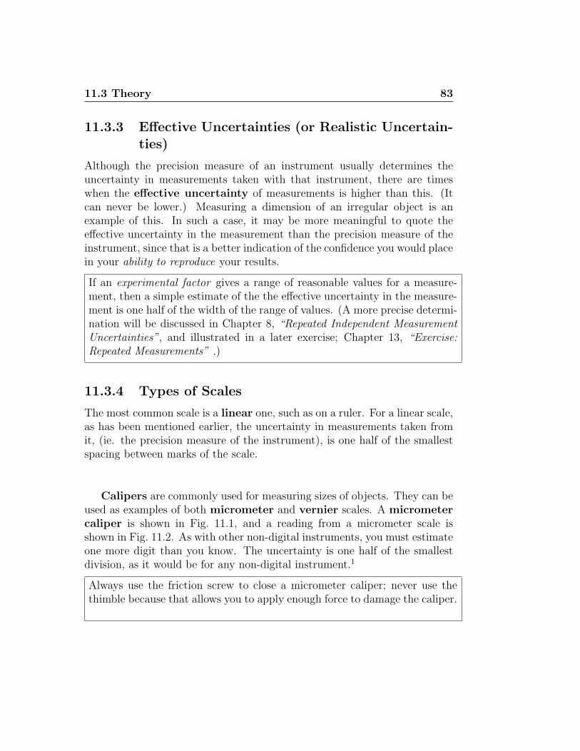
11.3 Theory 83

11.3.3 Effective Uncertainties (or Realistic Uncertain-ties)

Although the precision measure of an instrument usually determines theuncertainty in measurements taken with that instrument, there are timeswhen the effective uncertainty of measurements is higher than this. (Itcan never be lower.) Measuring a dimension of an irregular object is anexample of this. In such a case, it may be more meaningful to quote theeffective uncertainty in the measurement than the precision measure of theinstrument, since that is a better indication of the confidence you would placein your ability to reproduce your results.

If an experimental factor gives a range of reasonable values for a measure-ment, then a simple estimate of the the effective uncertainty in the measure-ment is one half of the width of the range of values. (A more precise determi-nation will be discussed in Chapter 8, “Repeated Independent MeasurementUncertainties”, and illustrated in a later exercise; Chapter 13, “Exercise:Repeated Measurements” .)

11.3.4 Types of Scales

The most common scale is a linear one, such as on a ruler. For a linear scale,as has been mentioned earlier, the uncertainty in measurements taken fromit, (ie. the precision measure of the instrument), is one half of the smallestspacing between marks of the scale.

Calipers are commonly used for measuring sizes of objects. They can beused as examples of both micrometer and vernier scales. A micrometercaliper is shown in Fig. 11.1, and a reading from a micrometer scale isshown in Fig. 11.2. As with other non-digital instruments, you must estimateone more digit than you know. The uncertainty is one half of the smallestdivision, as it would be for any non-digital instrument.1

Always use the friction screw to close a micrometer caliper; never use thethimble because that allows you to apply enough force to damage the caliper.

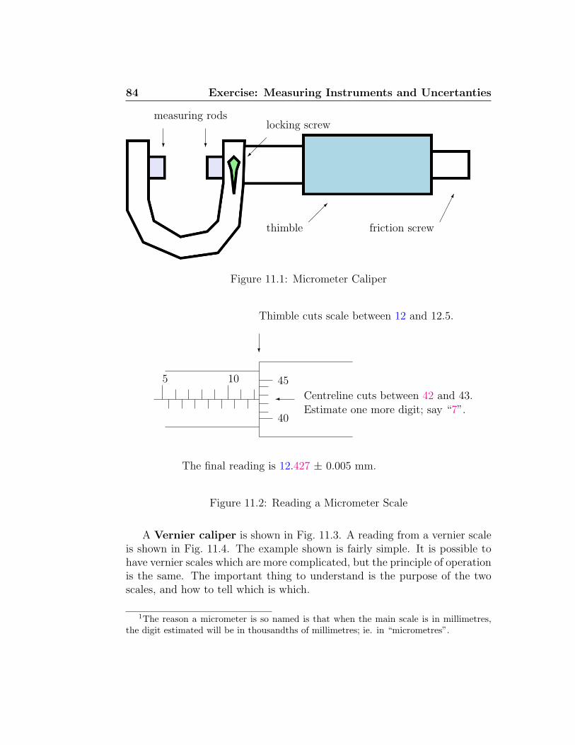
84 Exercise: Measuring Instruments and Uncertanties

? ?

measuring rods

��

locking screw

���

thimble����

friction screw

Figure 11.1: Micrometer Caliper

?

Thimble cuts scale between 12 and 12.5.

� Centreline cuts between 42 and 43.Estimate one more digit; say “7”.

40

45105

The final reading is 12.427 ± 0.005 mm.

Figure 11.2: Reading a Micrometer Scale

A Vernier caliper is shown in Fig. 11.3. A reading from a vernier scaleis shown in Fig. 11.4. The example shown is fairly simple. It is possible tohave vernier scales which are more complicated, but the principle of operationis the same. The important thing to understand is the purpose of the twoscales, and how to tell which is which.

1The reason a micrometer is so named is that when the main scale is in millimetres,the digit estimated will be in thousandths of millimetres; ie. in “micrometres”.

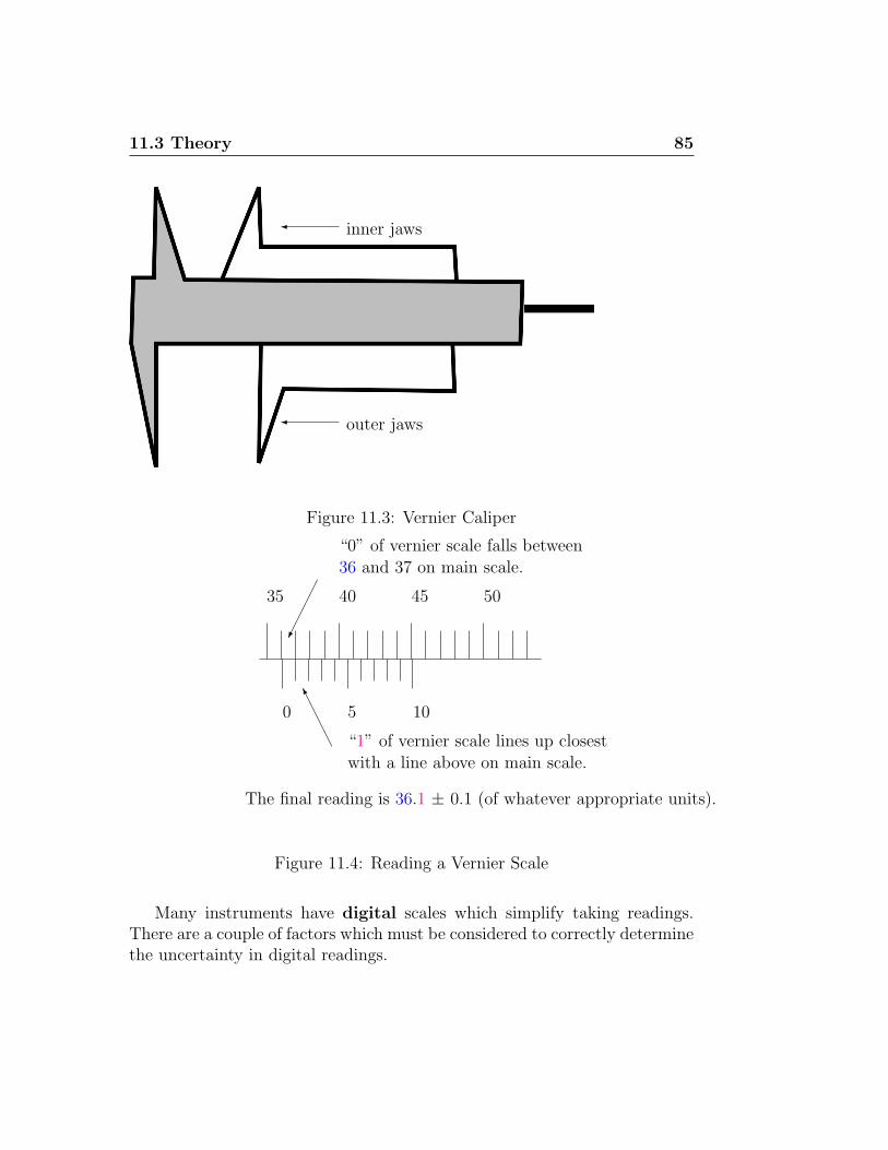
11.3 Theory 85

� inner jaws

� outer jaws

Figure 11.3: Vernier Caliper

35 ��

���

“0” of vernier scale falls between36 and 37 on main scale.

40 45 50

0

AA

AAK

“1” of vernier scale lines up closestwith a line above on main scale.

5 10

The final reading is 36.1 ± 0.1 (of whatever appropriate units).

Figure 11.4: Reading a Vernier Scale

Many instruments have digital scales which simplify taking readings.There are a couple of factors which must be considered to correctly determinethe uncertainty in digital readings.

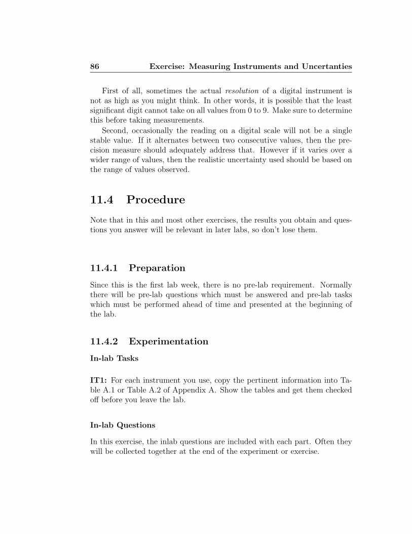
86 Exercise: Measuring Instruments and Uncertanties

First of all, sometimes the actual resolution of a digital instrument isnot as high as you might think. In other words, it is possible that the leastsignificant digit cannot take on all values from 0 to 9. Make sure to determinethis before taking measurements.

Second, occasionally the reading on a digital scale will not be a singlestable value. If it alternates between two consecutive values, then the pre-cision measure should adequately address that. However if it varies over awider range of values, then the realistic uncertainty used should be based onthe range of values observed.

11.4 Procedure

Note that in this and most other exercises, the results you obtain and ques-tions you answer will be relevant in later labs, so don’t lose them.

11.4.1 Preparation

Since this is the first lab week, there is no pre-lab requirement. Normallythere will be pre-lab questions which must be answered and pre-lab taskswhich must be performed ahead of time and presented at the beginning ofthe lab.

11.4.2 Experimentation

In-lab Tasks

IT1: For each instrument you use, copy the pertinent information into Ta-ble A.1 or Table A.2 of Appendix A. Show the tables and get them checkedoff before you leave the lab.

In-lab Questions

In this exercise, the inlab questions are included with each part. Often theywill be collected together at the end of the experiment or exercise.

11.4 Procedure 87

Precision Measure

• Linear Scales

IQ1: Sketch the portion of the instrument around your reading andgive the reading shown in your sketch with its uncertainty. Be sure toquote the correct number of significant figures in your measurement.

• GL1002R Balance

1. Press the tare button and write down the reading produced. Doesthe reading change over time? If so, record the first five valuesgiven.

2. Put the cup on the balance. Record the mass. Slowly add shot tothe cup, and record the mass when the reading changes.

3. Add more shot, until the reading changes again and determinewhat the smallest increment is which will be recognized.

IQ2: What is the precision measure of this balance? Is it what onemight expect just from looking at the balance? Explain.

• Stopwatch

Start and stop the watch several times to see if all digits are possibleas the least significant digit.

IQ3: Start the watch and try to stop it when it reaches 10 seconds.Give the reading obtained with its uncertainty. Be sure to quote thecorrect number of significant figures in your measurement.

Zero Error

• Spring Scale

IQ4: Sketch the portion of the spring scale near zero, and give thezero error with its uncertainty. State whether the zero error shouldbe added or subtracted to subsequent readings. Be sure to hang thescale vertically to determine the zero error, and explain why this isimportant.

88 Exercise: Measuring Instruments and Uncertanties

• Micrometer Caliper

IQ5: Sketch the portion of the micrometer caliper near zero, and givethe zero error with its uncertainty. State whether the zero error shouldbe added or subtracted to subsequent readings. Be sure to use thefriction screw when closing the micrometer to avoid damaging it.

Effective (or Realistic) Uncertainties

• From “Translational Equilibrium”, (Station 1)

– For the ramp, adjust the angle until the block slides down atconstant velocity once it has been tapped to get it started. Recordthe angle and the precision measure.

– Adjust the angle and find the limits of what could be considered“constant velocity”.

IT2: Record at least 3 experimental factors leading to uncertaintyin Table 11.3 along with bounds and indication of whether they arerandom, systematic, or possibly both.

IQ6: What is the effective uncertainty in the angle, due to determining“constant velocity”?

• From “Translational Equilibrium”, (Station 2)

– For the hanging masses in equilibrium, record the masses, theirangles, and the precision measure of the protractor.

– Displace the system from equilibrium, and let it come to restagain. Record the angles again. Repeat this by displacing thesystem in different ways.

IT3: Record at least 3 experimental factors leading to uncertaintyin Table 11.3 along with bounds and indication of whether they arerandom, systematic, or possibly both.

IQ7: What is the effective uncertainty in the angles based on this?

11.5 Bonus: Human Precision 89

– How much of an uncertainty in the angle is due to the string width?How much of an uncertainty in the angle is due to the difficultyin lining up the protractor? Are either of these significant giventhe previous factor?

IQ8: Combining all of these factors, what is the effective uncertaintyin the angles, and what factor is mainly responsible?

IT4: Show each of the completed tables in the template and get them checkedoff before you leave the lab.

11.4.3 Follow-up

Post-lab Tasks

T1: Go to the first URL given on the lab page to find diagram with partsof a micrometer labeled. Print the diagram.

T2: Go to the second URL given on the lab page to find diagram with partsof a micrometer labeled. Add the alternate names to the first diagram.

11.5 Bonus: Human Precision

For either mass or distance, determine your own “precision” by seeing howsmall a difference between two objects you can consistently detect. Explainhow you do this before you draw any conclusions.

Does your precision depend on an object’s dimensions or is it basicallyconstant?

11.6 Weightings

In-lab Questions and Tasks 80Post-lab Questions and Tasks 15Template 5Bonus 5

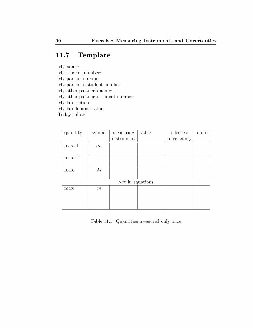
90 Exercise: Measuring Instruments and Uncertanties

11.7 Template

My name:My student number:My partner’s name:My partner’s student number:My other partner’s name:My other partner’s student number:My lab section:My lab demonstrator:Today’s date:

quantity symbol measuring value effective unitsinstrument uncertainty

mass 1 m1

mass 2

mass M

Not in equationsmass m

Table 11.1: Quantities measured only once

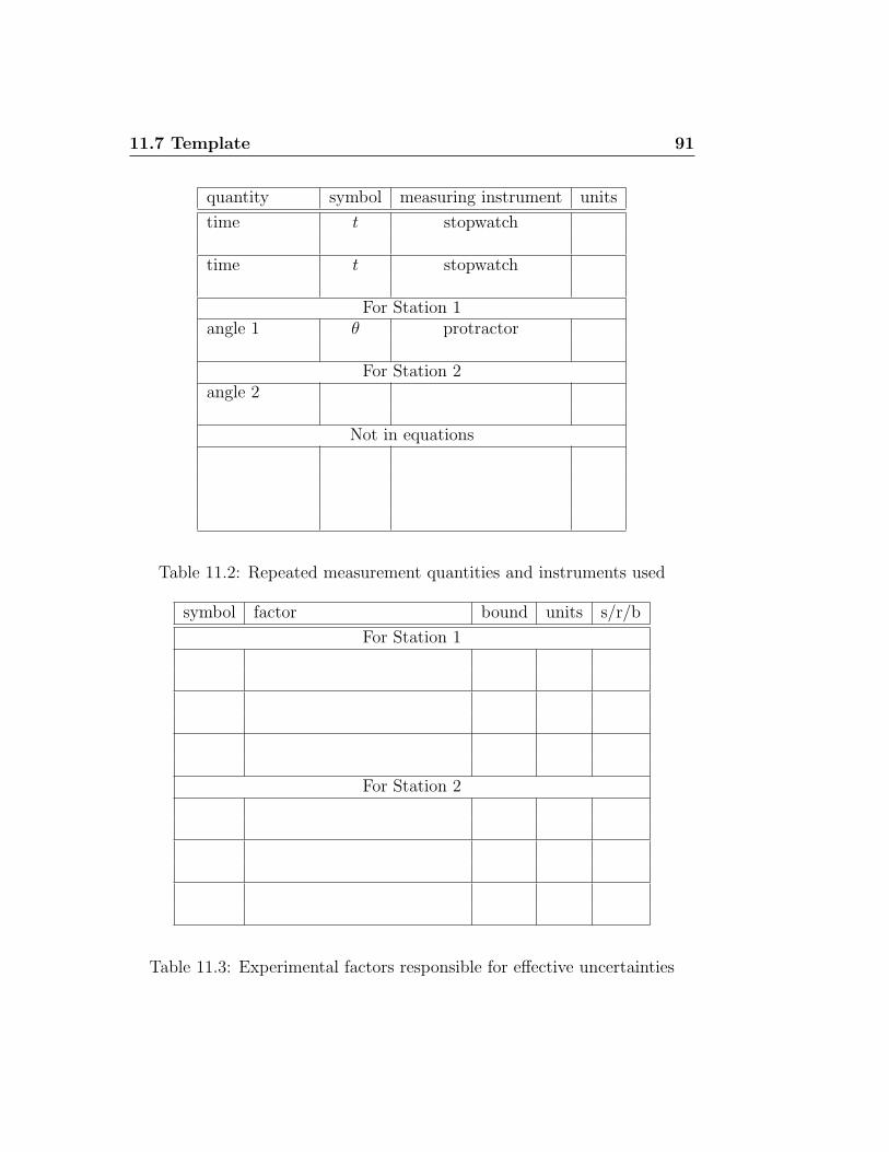
11.7 Template 91

quantity symbol measuring instrument units

time t stopwatch

time t stopwatch

For Station 1angle 1 θ protractor

For Station 2angle 2

Not in equations

Table 11.2: Repeated measurement quantities and instruments used

symbol factor bound units s/r/b

For Station 1

For Station 2

Table 11.3: Experimental factors responsible for effective uncertainties

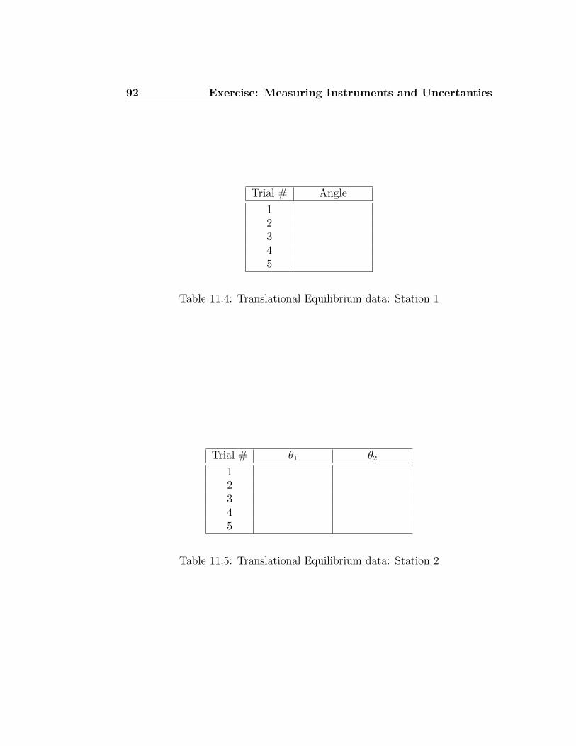
92 Exercise: Measuring Instruments and Uncertanties

Trial # Angle

12345

Table 11.4: Translational Equilibrium data: Station 1

Trial # θ1 θ2

12345

Table 11.5: Translational Equilibrium data: Station 2

Chapter 12

Exercise: Determining HumanReaction Time

12.1 Purpose

The purpose of the exercise is to determine reasonable measurements of hu-man reaction time, as it is a source of uncertainty in many experiments.

12.2 Introduction

This exercise will illustrate how to place bounds on a source of uncertaintywhich can be used in many experiments. Many of these results can be illus-trated with bar graphs for comparison purposes.

12.3 Theory

There are many different situations where human reaction time is important,but there are several different types of reactions which may be considered,and which have different times. Some of the possibilities are:

1. Time to react to a random event: this includes situations like hittingthe brakes in a vehicle when a child runs onto the street.

2. Time to react to an anticipated event: this includes situations likebatting a baseball as it crosses home plate.

94 Exercise: Determining Human Reaction Time

There are other related things to consider, such as how closely in time peo-ple may synchronize their actions with other events and/or people, and thepossibility of changes to these times with practice.

12.3.1 Random Events

Since one cannot anticipate a random event, by definition, there will be afinite time required for a reaction after the event happens.

12.3.2 Anticipated Events

When an event is anticipated, “reaction” does not necessarily follow theevent. In the example of hitting a baseball, it is possible for a batter to swingbefore the ball crosses the plate, (and in fact success requires the swing tobegin early), as easily as it is to swing after the ball crosses the plate.

12.3.3 Synchronization

In some situations, people must work together at a task, and then theymust try to synchronize their actions. In that case, there is a limitationto their ability to act together, and that also reflects a collective reactiontime. An example of this is musicians in an orchestra playing in time withthe conductor’s baton. A small time difference (either positive or negative)between the motion of the baton and the playing of different instrumentsturns “music” into “noise”.

12.3.4 Repeatability

No matter which situation occurs involving reaction time, it may be possiblefor experience to lead to an improvement. Drivers, batters, and musicianscan all perform better as they develop focus and experience.

12.4 Procedure 95

12.4 Procedure

12.4.1 Preparation

Pre-lab Questions

PQ1: Read through this exercise, and explain what it means for two rangesof numbers to obviously differ. Give an example of two ranges which don’tobviously differ, and give an example of two ranges which do obviously differ.(You can use ranges of 3 numbers for each example.)

Pre-lab Tasks

PT1: Go to the URL listed on the lab web page, and do the reaction timetest there. Print off the results and bring them to the lab to compare withthe results you produce in the lab.

PT2: Copy the results from PT1 into one column of Table 12.2.

PT3: Print off the “template” sheet of the spreadsheet for this exercise andbring it to the lab.

12.4.2 Experimentation

In-lab Questions

In this exercise, the in-lab questions are included with each part. Often theywill be collected together at the end of the experiment or exercise.

In-lab Tasks

IT1: For the instrument you use, copy the pertinent information into Ta-ble A.2 of Appendix A and fill in Table 12.1.

Random Events

1. Do several (at least 5) trials of the random event test and record thetimes. Any negative times are basically “wild guesses” and should beignored.

96 Exercise: Determining Human Reaction Time

2. Repeat with the other partner.

IQ1: Was one person’s reaction time obviously1 longer than the other’s?

Anticipated Events

1. Do several trials of the anticipated event test and record the times.Negative times are educated guesses and should be included.

2. Repeat with the other partner.

IQ2: Was one person’s reaction time obviously longer than the other’s?

SynchronizationUsually synchronization involves one person being the initiator and the

other being the responder (like the conductor and a musician).

1. Figure out a method to try and synchronize with each other.

2. Do several trials of the synchronization test and record the times.

3. Repeat with the roles of “initiator” and “responder” reversed.

IQ3: Was there any obviously better choice of which person to initiate?

RepeatabilityThis applies to all of the previous situations.

1. Look at your previous data sets and see if the times are changing ac-cording to a pattern in any of them.

IQ4: Was there any indication that something was changing systematicallyas trials went on? (For instance, were times getting shorter or longer?) If so,what insight does this give about doing an experiment?

IT2: For each instrument you use, copy the pertinent information into Ta-ble A.1 or Table A.2 of Appendix A. Show the tables and get them checkedoff before you leave the lab.

IT3: Show the template tables and get them checked off before you leavethe lab.

1If the ranges of two sets of times don’t overlap, then they obviously differ.

12.5 Bonus: Other Factors to Study 97

12.4.3 Analysis

Post-lab Discussion Questions

These questions will only be able to be completed after the “Repeated Mea-surements” lab exercise has been completed.

Q1: Did the two reaction times for random events for the two people agreewithin experimental uncertainty?

Q2: Did the two reaction times for anticipated events for the two peopleagree within experimental uncertainty?

Q3: Was either person’s reaction time for anticipated events equal to zerowithin experimental uncertainty?

Q4: Did the two synchronization times for the two situations agree withinexperimental uncertainty?

Q5: Was either synchronization time equal to zero within experimental un-certainty? How did your synchronization times compare to your anticipatedtimes?

Q6: Which measurement of reaction time do you feel most closely approx-imates the situation when the ball was being dropped? Is there more thanone? Was there any correspondence between reaction times you measuredand the variation in times you got when dropping the ball?

Q7: How did your reaction time from the pre-lab exercise compare with thevalue you got in the lab?

12.5 Bonus: Other Factors to Study

Choose any one of the following (depending on equipment available):

1. See if it matters whether a button is pushed or released to stop thetime.

2. See if the time taken between repetitions makes a difference.

3. Determine whether the mode of stimulus matters (eg. sight versussound).

98 Exercise: Determining Human Reaction Time

4. Determine whether practice does indeed make perfect by doing manyrepetitions of a test (at least 30) to see if results improve.

5. Figure out whether the length of the sequence for an anticipated eventmatters.

6. Figure out whether the speed of the sequence for an anticipated eventmatters.

7. Test whether the method of synchronization can be improved.

8. Check whether any person in the lab is significantly better or worse forthe anticipated event.

9. Check whether any group in the lab is significantly better or worse forsynchronization.

10. Check whether musical ability influences synchronization.

11. Check whether athletic ability influences synchronization.

12. (For musicians) Given the suggested tempo and time signature of apiece of music, determine the maximum synchronization delay allow-able for a performance.

12.6 Weightings

Pre-lab Questions and Tasks 10In-lab Questions and Tasks 40Post-lab Questions and Tasks 45Template 5Bonus 5

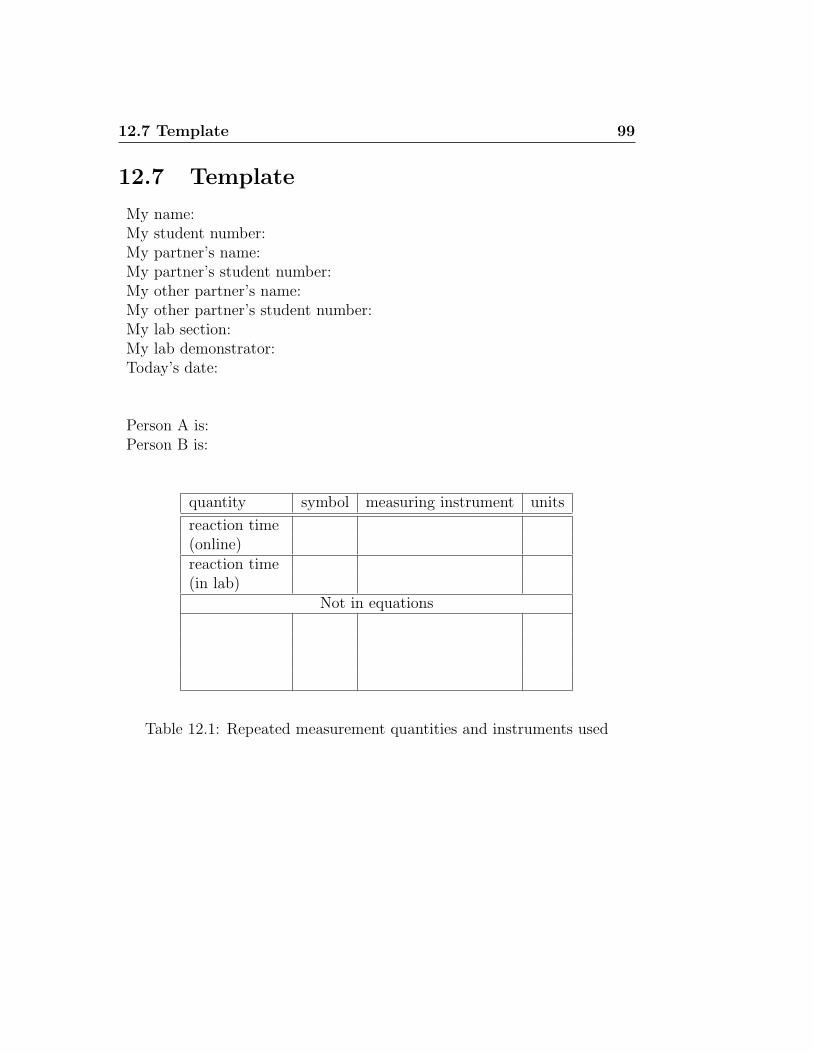
12.7 Template 99

12.7 Template

My name:My student number:My partner’s name:My partner’s student number:My other partner’s name:My other partner’s student number:My lab section:My lab demonstrator:Today’s date:

Person A is:Person B is:

quantity symbol measuring instrument units

reaction time(online)reaction time(in lab)

Not in equations

Table 12.1: Repeated measurement quantities and instruments used

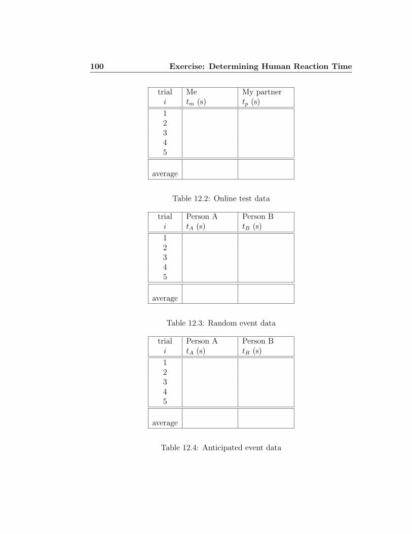
100 Exercise: Determining Human Reaction Time

trial Me My partneri tm (s) tp (s)

12345

average

Table 12.2: Online test data

trial Person A Person Bi tA (s) tB (s)

12345

average

Table 12.3: Random event data

trial Person A Person Bi tA (s) tB (s)

12345

average

Table 12.4: Anticipated event data

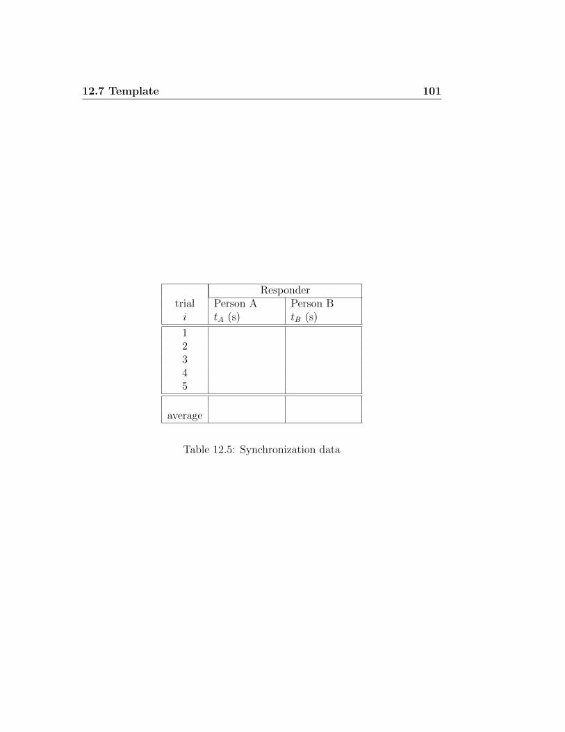
12.7 Template 101

Respondertrial Person A Person B

i tA (s) tB (s)

12345

average

Table 12.5: Synchronization data

102 Exercise: Determining Human Reaction Time

Chapter 13

Exercise: RepeatedMeasurements

13.1 Purpose

The purpose of this exercise is make you familiar with calculations involvingrepeated measurements.

13.2 Introduction

In this experiment, you will be introduced to the concepts repeated depen-dent and independent measurements.

13.3 Theory

Most of the “theory” for this experiment has been covered in Chapter 8; “Re-peated Independent Measurement Uncertainties” and Chapter 9; “RepeatedDependent Measurements with Constant Intervals” of the lab manual.

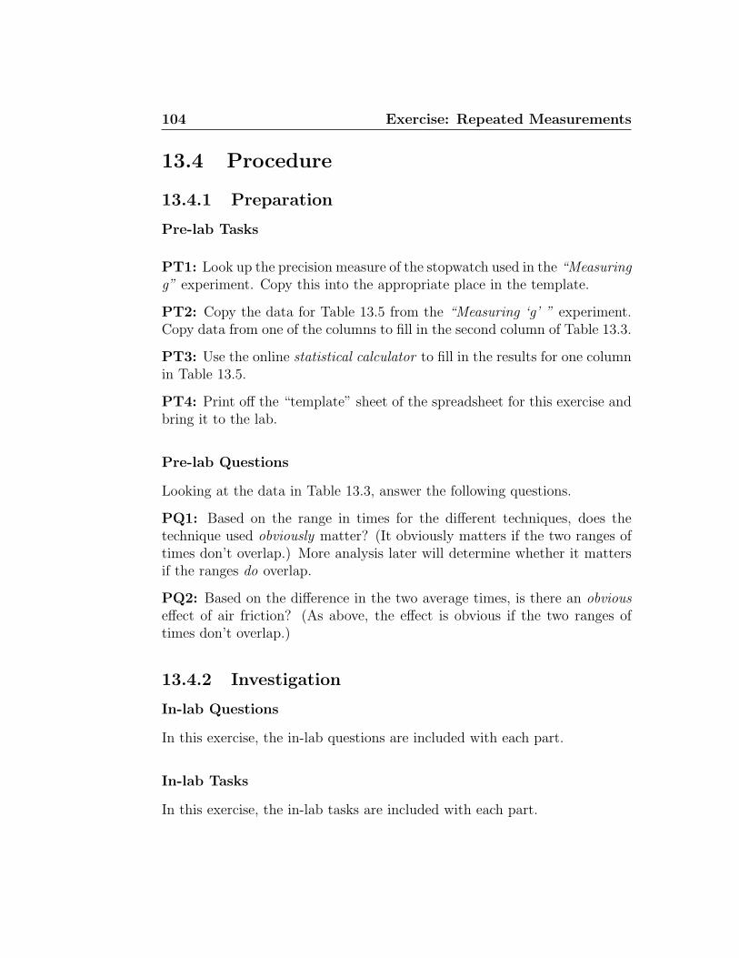
104 Exercise: Repeated Measurements

13.4 Procedure

13.4.1 Preparation

Pre-lab Tasks

PT1: Look up the precision measure of the stopwatch used in the “Measuringg” experiment. Copy this into the appropriate place in the template.

PT2: Copy the data for Table 13.5 from the “Measuring ‘g’ ” experiment.Copy data from one of the columns to fill in the second column of Table 13.3.

PT3: Use the online statistical calculator to fill in the results for one columnin Table 13.5.

PT4: Print off the “template” sheet of the spreadsheet for this exercise andbring it to the lab.

Pre-lab Questions

Looking at the data in Table 13.3, answer the following questions.

PQ1: Based on the range in times for the different techniques, does thetechnique used obviously matter? (It obviously matters if the two ranges oftimes don’t overlap.) More analysis later will determine whether it mattersif the ranges do overlap.

PQ2: Based on the difference in the two average times, is there an obviouseffect of air friction? (As above, the effect is obvious if the two ranges oftimes don’t overlap.)

13.4.2 Investigation

In-lab Questions

In this exercise, the in-lab questions are included with each part.

In-lab Tasks

In this exercise, the in-lab tasks are included with each part.

13.4 Procedure 105

Part 1: Independent Measurements

IT1: Fill in the rest of Table 13.3 and Table 13.4 to show how to do astatistical analysis. Use the data from the column of Table 13.5 which youused in the statistical calculator, so that you can confirm your results.

IQ1: Based on your calculated uncertainty, did the precision measure of thestop watch limit the precision of your average time for the chosen data set?Why or why not? This should be a question you can answer definitively basedon your statistical analysis.

IQ2: Approximately 2/3 of the values should vary from the average by lessthan the standard deviation. Does this hold true for one of your data sets?Explain why this might not always be so, even if it is the case for your results.

Part 2: Dependent Measurements

Using the “carts” software One of the challenges of using data col-lection software in the lab is to strike a balance between being easy to use andstill requiring students to think. Much of the commercial software availablewill collect data, plot graphs, etc. so students become passive observers andexperiments are really just demonstrations. The software used in this lab isvery simple so that collecting the data is all it does.

The consequence of the simplicity of this software is that there are veryfew assumptions made about the experiment. Specifically:

1. The ladder with 13 bars will be used for each cart. Thus 13 bars passingthrough a gate will be identified as a single “cart”.

2. “Before” and “after” refer to the gates, not to the possible collision.The first set of 13 times through a gate is designated “before” and anyothers are designated “after”.

3. Time “begins” when the first cart begins to pass through a gate. Alltimes are relative to this.

What these mean is that you have to think about which set(s) of times referto which cart(s) and at what point in the experiment. The only way to changethings would be to design the software with a particular type of collision inmind, which would make it easy to use but completely lacking in versatility.

106 Exercise: Repeated Measurements

1. Measure the “ladder” spacing of the setup for the “One DimensionalConservation of Momentum and Energy” experiment with the precisionmeasure of the instrument used.

In this case, when the spacing of the individual bars should be veryconsistent, the best way to determine the spacing is to measure thedistance for all thirteen bars, and divide in order to get the length ofany sub-interval. Be sure to count and measure intervals, not bars.

2. Perform the experiment as required, making sure that the track is aslevel as it can be made.

3. With the stopwatch, time how long it takes the cart to go one metre,and calculate the velocity to compare with later calculations.

IQ3: Sketch the ladder, showing what positions on the ladder you used tomeasure the spacing.

IQ4: Calculate the first difference and show how you did it.

IT2: Do an order of magnitude calculation for the velocity using a single timeinterval, and compare it to the velocity you calculated using the stopwatch.

13.4.3 Analysis

Post-lab Discussion Questions

In this exercise, the post-lab questions are included with each part.

“Measuring ‘g’ ”

1. Repeat the calculation of mean, standard deviation and standard de-viation of the mean for each of your sets of times.

2. Based on the value of α calculated, determine the number of additionalmeasurements needed in order to reduce α to the same size as thep.m. (Hint: Assume σ does not change significantly with additionalmeasurements.)

3. Create tables for your lab report, with proper titles, numbers, etc.

13.5 Bonus: Using Calculator Built-in Statistical Functions 107

4. For each table, record average time, the standard deviation, the stan-dard deviation of the mean, and the ultimate uncertainty in the averagetime.

Q1: Were the times given by different methods for the same ball significantlydifferent?

Q2: Were the times given by the preferred method for the first ball and thesecond ball significantly different?

Q3: Would it be feasible to take the number of measurements calculatedabove in the actual experiment?

Part 2: Dependent Measurements

13.4.4 Follow-up

Post-lab Tasks

T1: Calculate the average velocity of the cart using the method of differences,and state the result with its uncertainty.

T2: Can you tell from your data if the cart is accelerating or deccelerating?Explain.

13.5 Bonus: Using Calculator Built-in Sta-

tistical Functions

If your calculator has built–in functions to calculate averages and standarddeviations, test them out with the above data. Does your calculator calculatethe correct value for σ? If not, how can you correct it?

Write out the instructions needed to do this on your calculator. Includehow to clear for a new data set, and show what is in the display after eachinstruction for a sample. (Record the make and model of calculator youhave.) After you have verified the operation of the statistical functionson your calculator, you can use them whenever you need to calculate thesequantities.

108 Exercise: Repeated Measurements

13.6 Weightings

Pre-lab Questions and Tasks 10In-lab Questions and Tasks 40Post-lab Questions and Tasks 45Template 5Bonus 5

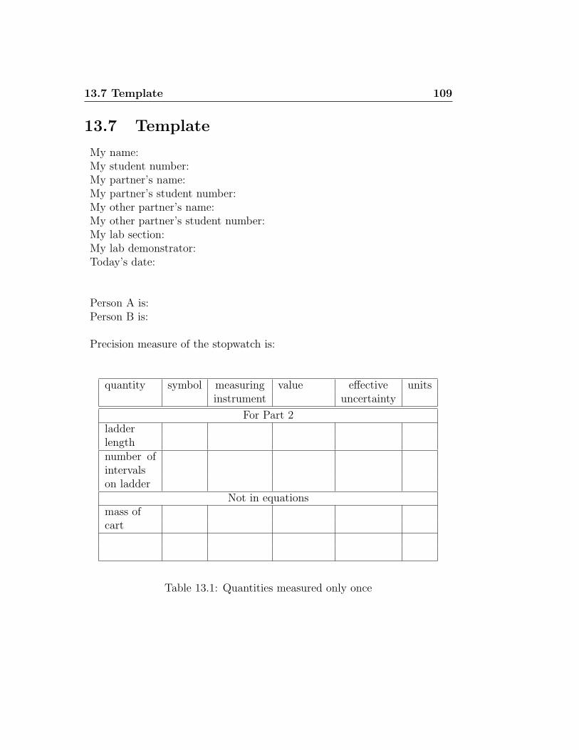
13.7 Template 109

13.7 Template

My name:My student number:My partner’s name:My partner’s student number:My other partner’s name:My other partner’s student number:My lab section:My lab demonstrator:Today’s date:

Person A is:Person B is:

Precision measure of the stopwatch is:

quantity symbol measuring value effective unitsinstrument uncertainty

For Part 2ladderlengthnumber ofintervalson ladder

Not in equationsmass ofcart

Table 13.1: Quantities measured only once

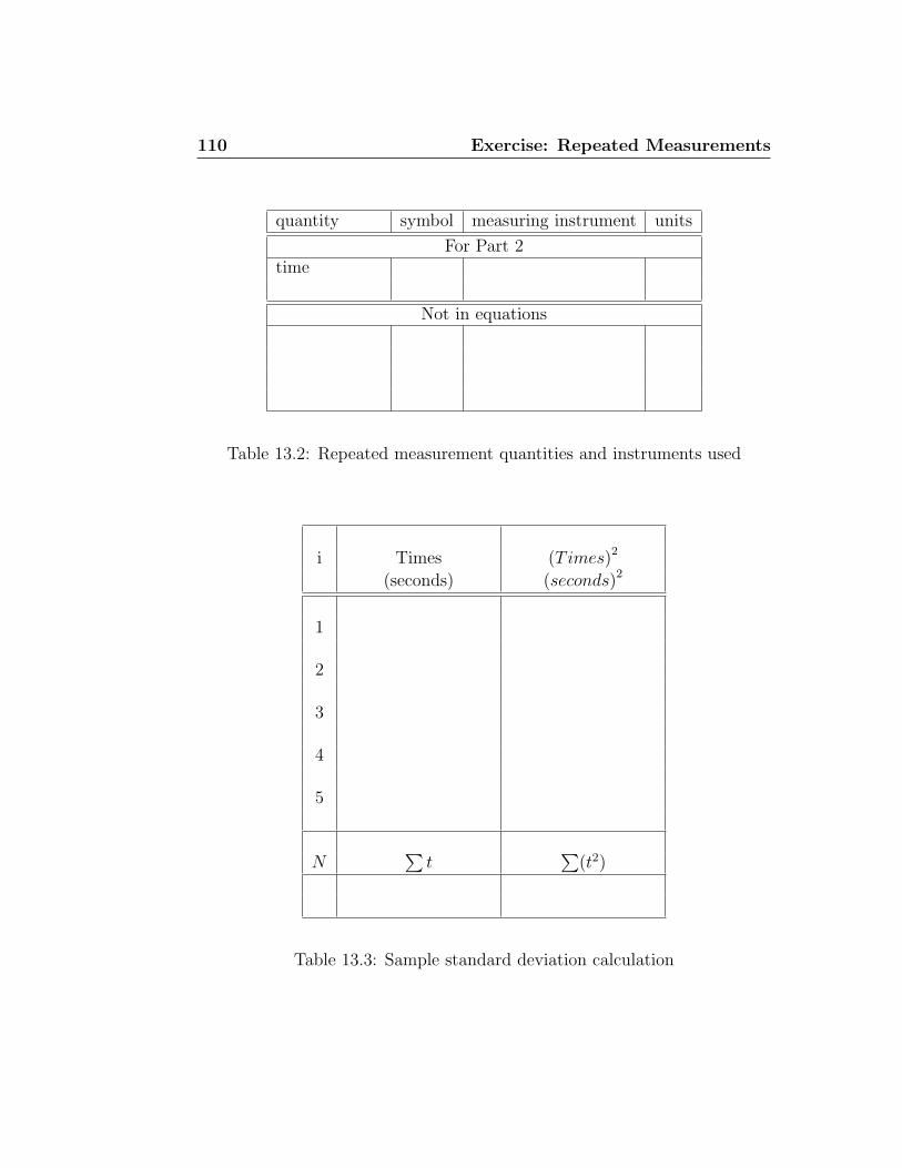
110 Exercise: Repeated Measurements

quantity symbol measuring instrument units

For Part 2time

Not in equations

Table 13.2: Repeated measurement quantities and instruments used

i Times (Times)2

(seconds) (seconds)2

1

2

3

4

5

N∑

t∑

(t2)

Table 13.3: Sample standard deviation calculation

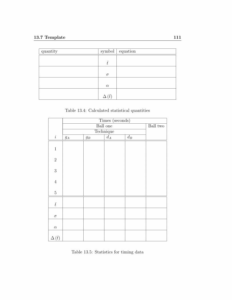
13.7 Template 111

quantity symbol equation

t̄

σ

α

∆ (t̄)

Table 13.4: Calculated statistical quantities

Times (seconds)Ball one Ball two

Techniquei gA gB dA dB

1

2

3

4

5

t̄

σ

α

∆ (t̄)

Table 13.5: Statistics for timing data

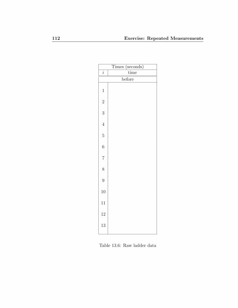
112 Exercise: Repeated Measurements

Times (seconds)i time

before

1

2

3

4

5

6

7

8

9

10

11

12

13

Table 13.6: Raw ladder data

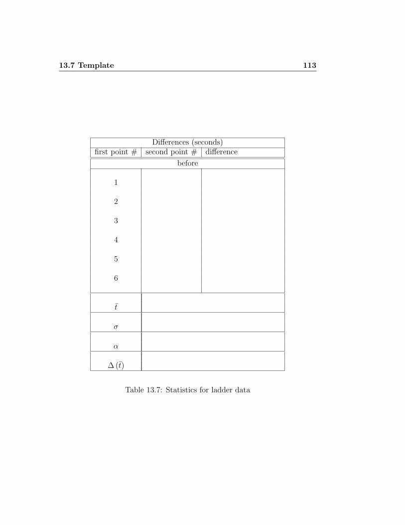
13.7 Template 113

Differences (seconds)first point # second point # difference

before

1

2

3

4

5

6

t̄

σ

α

∆ (t̄)

Table 13.7: Statistics for ladder data

114 Exercise: Repeated Measurements

Chapter 14

Exercise: ProcessingUncertainties

14.1 Purpose

The purpose of the exercise is to develop skills in calculating with uncer-tainties, recognizing significant sources of error, and writing a “Discussion”.Many of these results will be used in future labs, so be sure not to lose thisreport.

14.2 Introduction

This exercise should help you become familiar with calculations involvinguncertainties, and how to address them in lab reports.

The “Discussion of Errors” (or Uncertainties) section of a lab report iswhere you outline the reasonable limits which you place on your results. Ifyou have done a professional job of your research, you should be preparedto defend your results. In other words, you should expect anyone else to getresults which agree with yours; if not, you suspect theirs. In this context,you want to discuss sources of error which you have reason to believe aresignificant.

116 Exercise: Processing Uncertainties

14.3 Theory

This has been covered previously. (See Chapter 10, “Uncertain Results” inthe manual.)

14.3.1 Summary of Rules

Basic arithmetic rules

The uncertainty in results can usually be calculated as in the following ex-amples (if the percentage uncertainties in the data are small):

(a) ∆(A + B) = (∆A + ∆B)

(b) ∆(A−B) = (∆A + ∆B)

(c) ∆(A×B) ≈ |AB|(∣∣∆A

A

∣∣+ ∣∣∆BB

∣∣)(d) ∆(A

B) ≈

∣∣AB

∣∣ (∣∣∆AA

∣∣+ ∣∣∆BB

∣∣)Note that the first two rules above always hold true.

Uncertainties in functions, by algebra

∆f(x) ≈ |f ′(x)|∆x (14.1)

Uncertainties in functions, by inspection

∆f(x) ≈ fmax − f (14.2)

or

∆f(x) ≈ f − fmin (14.3)

Sensitivity of Total Uncertainty to Individual Uncertainties

If f = f(x, y), then to find the proportion of ∆f due to each of the individualuncertainties, ∆x and ∆y, proceed as follows:

• To find ∆fx, let ∆y = 0 and calculate ∆f .

• To find ∆f y, let ∆x = 0 and calculate ∆f .

14.3 Theory 117

Simplifying Uncertainties

You do not need to carry uncertainties through if they do not contributemore than 10% of the total uncertainty, since uncertainties are usually onlyexpressed to one decimal place. (However, be sure to give bounds for theseuncertainties when you do this.)

Uncertainties and Final Results

Mathematically, if two quantities a and b, with uncertainties ∆a and ∆b arecompared, they can be considered to agree within their uncertainties if

|a− b| ≤ ∆a + ∆b (14.4)

A value with no uncertainty given can be assumed to have an uncertainty ofzero.

If two numbers do not agree within experimental error, then the percentagedifference between the experimental and theoretical values must be calcu-lated as follows:

Percent Difference =

∣∣∣∣theoretical − experimental

theoretical

∣∣∣∣× 100% (14.5)

Remember: Only calculate the percent difference if your results do not agreewithin experimental error.

Significant Figures in Final Results

Always quote final answers with one significant digit of uncertainty, andround the answers so that the least significant digit quoted is the uncertainone.

14.3.2 Discussion of Uncertainties

• Spend most time discussing the factors which contribute most to un-certainties in your results.

118 Exercise: Processing Uncertainties

• Always give a measured value or a numerical bound on an uncertainty.

• State whether any particular factor leads to a systematic uncertaintyor a random one. If it’s systematic, indicate whether it would tend toincrease or decrease your result.

Types of Errors

• Measurable uncertainties

• Bounded uncertainties

• Blatant filler

Dont’t use “human error”; it’s far too vague.

Reducing Errors

1. Avoid mistakes.

2. Repeat for consistency, if possible.

3. Change technique

4. Observe other factors as well; including ones which you may have as-sumed were not changing or shouldn’t matter.

5. Repeat and do statistical analysis.

6. Change equipment; the last resort.

Ridiculous Errors

Anything which amounts to a mistake is not a valid source of error. A seriousscientist will attempt to ensure no mistakes were made before consideringreporting on results.

14.4 Procedure 119

14.4 Procedure

14.4.1 Preparation

Pre-lab Tasks

PT1: Copy the data into Table 14.1 from the results of the “Repeated Mea-surements” exercise.

PT2: Rearrange the equation to solve for g as required in IQ1.

PT3: Use the online uncertainty calculator to fill in the results for onecolumn in Table 14.1 using the method of maximum uncertainty.

PT4: What was the precision measure of the stopwatch from “Measuring‘g’ ”? Copy this value into the template.

PT5: What were the height and the realistic uncertainty in the height from“Measuring ‘g’ ”, and what factor(s) caused the uncertainty? Copy thesevalues into the template.

Pre-lab Questions

PQ1: For each of the following situations, come up with a physically plausi-ble explanation in a sentence or so. (Mistakes in calculations do not count asphysically plausible, unless they are errors with units or constants. System-atic errors in measurements are valid, but you must specify in what directionan error must be to have the effect observed.) If you suggest a scale error forone situation, don’t simply use the opposite error for the opposite case. (ie.Try to come up with different things.)

• Values for g for both the dense and the non-dense ball are below theexpected value of 9.8m/s2.

• Values for g for both the dense and the non-dense ball are above theexpected value of 9.8m/s2.

• The value for g for dense ball is above the expected value of 9.8m/s2,but the value for g for the non-dense ball is below the expected valueof 9.8m/s2.

120 Exercise: Processing Uncertainties

PQ2: Can you think of any obvious mistake which might result in gettingthe value for g for dense ball below the expected value of 9.8m/s2, but thevalue for g for the non-dense ball above the expected value of 9.8m/s2?(Hint: Consider the case where the values for g were not calculated when theexperiment was performed, but some days or weeks later.)

14.4.2 Investigation

In-lab Questions

IQ1: (From “Measuring ‘g’ ”)

• h = 12gt2

• Find the equation for ∆g by both methods; (algebra and inspection).State which method you preferred and why.

(Note: you will first have to rearrange the equation.)

• Using either method, determine the equations for ∆gh and ∆gt.

• Using your actual data, and the results from previous exercises, findthe numerical values of∆g for one data set by both methods. Do thetwo methods agree when rounded to one significant figure?

• Using your actual data, find the numerical values of the sensitivity of∆g to each of the quantities involved, (ie. ∆gh and ∆gt), based on yourdata for the same data set.

For the “Measuring g” experiment, answer the following questions. Don’tdiscuss an uncertainty unless you have given a measured value or an esti-mated bound for it.

IQ2: From your numerical results for the uncertainty in g, which quantity,(h or t), produced the biggest proportional effect? In other words, which wasbigger; ∆gh or ∆gt?

IQ3: From the answer to question 2, what experimental factor from thosediscussed when you collected the data made the biggest contribution to theuncertainty in the quantity mentioned?

14.4 Procedure 121

IQ4: From the answer to question 3, what steps might be taken to reducethe uncertainty, keeping in mind the guidelines about the best ways to reduceuncertainties from earlier in this exercise?

IQ5: For the quantity not used in question 2, what factor from those dis-cussed when you collected the data made the biggest contribution to theuncertainty in the quantity, and what steps might be taken to reduce theuncertainty, keeping in mind the guidelines about the best ways to reduceuncertainties?

IQ6: Are there any other factors which contributed significantly to the un-certainty in your result? If so, how do they affect the results and what canbe done to reduce them?

14.4.3 Analysis

Post-lab Discussion Questions

All of the in-lab questions from this exercise should be incorporated into yourDiscussion for “Measuring ‘g’ ”, as should be the case for all of the exerciseswhich contributed to completing the “Measuring ‘g’ ” lab report.

14.4.4 Follow-up

Post-lab Tasks

T1: Fill in the rest of Table 14.1 and determine the most important sourceof uncertainty for each data set.

For tasks T2 to T5: In each of the following equations, assume each of thequantities has an uncertainty associated with it, and calculate the uncertaintyin the result two ways;

1. algebraically

2. by inspection (or trial-and-error, if it’s not easy otherwise), determin-ing which signs for all of the variables gives the biggest change fromthe quantity without uncertainties. (Be sure to state any assumptionsabout the signs of quantities involved.)

122 Exercise: Processing Uncertainties

T2: (From “Translational Equilibrium”)

• Tx = T cos θ

• Given uncertainties ∆T , ∆θ

• Find ∆Tx by both methods. State which you preferred.

• Hand in these answers, and copy the equation into Table 19.4.

Note: when dealing with angles, ALWAYS convert to radians first. Evenspreadsheets are set up to use radians, not degrees! The reason this is im-portant for uncertainties is shown by the following example:Suppose

A = sin (θ)

then∆A = |cos (θ)|∆θ

The last term, ∆θ, will be different depending on whether the angle is indegrees or radians, and must be in radians for the result to be correct.

The following ones will probably be easiest if you treat them as twoseparate terms and then add the results.

T3: (From “One Dimensional Conservation of Momentum and Energy”)

• P = m1v1 + m2v2

• Given uncertainties ∆m1, ∆v1, ∆m2, ∆v2

• Find ∆P by both methods. State which you preferred.

• Hand in these answers, and copy the equation into Table 20.4.

T4: (From “One Dimensional Conservation of Momentum and Energy”)

• E = 12m1v

21 + 1

2m2v

22

• Given uncertainties ∆m1, ∆v1, ∆m2, ∆v2

• Find ∆E by both methods. State which you preferred.

• Hand in these answers, and copy the equation into Table 20.4.

14.5 Bonus 123

T5: (From “Moment of Inertia”)

• I = 12m (r2

1 + r22)

• Given uncertainties ∆m, ∆r1, ∆r2

• Find ∆I by both methods. State which you preferred.

• (Hint: In this case, multiply it out to get two separate terms, and thenproceed as above.)

• Hand in these answers, and copy the equation into Table 18.6.

14.5 Bonus

14.5.1 Proof of earlier result; uncertainty in marblevolume

This question is from the “Uncertain Results” section of the manual.For a sphere,

V =4

3π

(d

2

)3

and so by inspection

∆V ≈ 4

3π

(d + ∆d

2

)3

− 4

3π

(d

2

)3

Algebraically,

V ′ = 2π

(d

2

)2

=π

2d2

and so

∆V ≈∣∣∣π2d2∣∣∣∆d

Show that these two methods give the same results if uncertainties are small;ie. if ∆d << d. Remember that uncertainties in final results are usually onlyexpressed to one decimal place, so you can usually discard terms with twoor more ∆ terms multiplied together; for instance ∆A∆B ≈ 0

124 Exercise: Processing Uncertainties

14.6 Weightings

Pre-lab Questions and Taks 10In-lab Questions and Tasks 60Post-lab Questions and Tasks 25Template 5Bonus 5

14.7 Template 125

14.7 Template

My name:My student number:My partner’s name:My partner’s student number:My other partner’s name:My other partner’s student number:My lab section:My lab demonstrator:Today’s date:

g has units of:The equation used for ∆g is:

h has a value (with units) of:The realistic uncertainty in h is:

The precision measure of the stopwatch (including units) was:

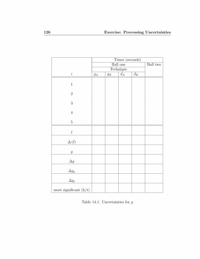
126 Exercise: Processing Uncertainties

Times (seconds)Ball one Ball two

Techniquei gA gB dA dB

1

2

3

4

5

t̄

∆ (t̄)

g

∆g

∆gh

∆gt

most significant (h/t)

Table 14.1: Uncertainties for g

Chapter 15

Exercise: Introduction toSpreadsheets

15.1 Purpose

The purpose of this exercise is to introduce you to the use of a spreadsheetas a tool for data analysis.

15.2 Introduction

A spreadsheet is basically a large programmable calculator with some specialfeatures thrown in. Because of this it is very useful for data analysis. It isimportant that you try to learn how to use the spreadsheet, rather than simplytry to “get the work done”. A spreadsheet is a handy tool, and these labsgive you an opportunity to become familiar with it, if you are not already.It will be well worth the effort to use a spreadsheet for calculations for thetime saved and mistakes avoided as you become more experienced with it.(Ask your lab demonstrator!).

15.3 Theory

Some of the information here will be specific to Microsoft Excel, but mostshould be similar for other spreadsheets as well.

128 Exercise: Introduction to Spreadsheets

15.3.1 Formulas

The value in using cell references instead of numerical values is that if thenumbers change, the calculations are performed automatically. In a lab thisallows you to set up the spreadsheet and then simply type in new data to seenew results. If you do things properly, it is even easy to change the numberof data points after the fact.

Never use a number where you can use a cell reference.

15.3.2 Functions

Functions perform commonly used tasks on a cell or block of cells and returnthe result in a cell.1 Some of the most common ones follow.

Common Functions

For blocks of cells

• average()

• count() counts the non-empty cells

Always use the count function instead of typing in the number of data pointsso you can change the number later if needed without editing formulas.

• stdeva() determines the sample standard deviation

• max() finds the maximum

• min() finds the minimum

For individual values

• sqrt() square root

• abs() absolute value

• if() allows a cell to have a value depending on a condition

1There are functions which return a block of cells, which don’t fit with the mathematicalnotion of a “function”, but we won’t get into those here.

15.3 Theory 129

Using the Built-in Automation

In you aren’t sure what parameters are needed by a function, or in whatorder, you can simply type in the function until after the left bracket andthen you will be prompted for what needs to be filled in.

15.3.3 Copying Formulas and Functions: Absolute andRelative References

Never copy values from one part of the spreadsheet to another where a cellreference could be used instead.

Relative References

The value of using formulas in a spreadsheet is that calculations can be easilyrepeated. One of the ways this happens is by copying formulas to be appliedto different data. When a formula is copied from one location to another,references are usually changed relative to the move. In other words, if aformula is copied from one cell to the next one on the right (ie. where thecolumn address increases by one), then cell references within the formulawill have their column addresses increased by one as well. If a formula iscopied from one cell to the one above (ie. where the row address decreasesby one), then cell references within the formula will have their row addressesdecreased by one as well.2

Absolute References

Sometimes you don’t want cell references in a formula to change when itis copied. In this case what you do is to put a $ before the part of a cellreference which you do not want to change. in other words, if you have aformula with a reference to B13 and you do not want the B to change whenyou copy, then change the reference to $B13. If you don’t want the 13 tochange when you copy, then change the reference to B$13. If you don’t wanteither B or 13 to change, then change the reference to $B$13. (In otherwords, you make a number a constant by referring to it like $B$13).

2Note that when you move a cell, none of the references inside it are changed.

130 Exercise: Introduction to Spreadsheets

15.3.4 Pasting Options

Sometimes when you copy a formula, you don’t want to copy everythingabout it. For instance, sometimes you just want to get the numerical result.In a spreadsheet, you can’t choose what to copy, but you can choose what topaste. When you go to paste something, you can Paste Special and chooseto paste whatever you want. Thus you can paste strings or numbers and notformulas, and you can include formatting (boxes, colours, fonts, etc.) or not.

Always copy formulas from one part of the spreadsheet to another instead ofretyping to avoid making mistakes.

15.3.5 Formatting

You can do many things to a cell or block of cells to change its appearance,such as putting boxes around it, changing fonts or how numbers are displayed,changing the background colour, etc.

Format after you’re done copying formulas, etc., to avoid having to alwaysPaste Special to preserve style information.

15.3.6 Print Preview

When printing a spreadsheet, there are lots of options to make the resultmore readable. Doing a print preview allows this. You can

• turn the grid off.

• include page headers and footers (or not)

• scale to fit the page

Doing a page preview also helps you figure out which page number(s) youneed to print, since it may not be obvious.

Preview the printing to avoid wasting reams of paper printing out stuff youdon’t want.

15.4 Procedure 131

15.4 Procedure

15.4.1 Preparation

You are welcome to go ahead and do as much of the exercise on your ownas you wish; you can just bring your spreadsheet with you to the lab anddemonstrate the points indicated. If you get it all done in advance, that’sgreat.

If you do it on your own, then print a copy of the spreadsheet showingformulas along with the ones indicated in the post-lab questions. (You onlyneed to show the formulas for rows mentioned in the instructions.)

Pre-lab Tasks

PT1: Follow the link posted on the web site to create a Novell login beforethe lab. Verify that you can log in to a computer in one of the public labson campus before you come to the lab.

15.4.2 Investigation

In-lab Tasks

In this exercise, the in-lab tasks are included with each part.

Creating the First Formulas

1. Cell B14 should containg the average for the steel ball. In that cell,begin by typing a “=” so Excel knows you’re typing a formula. Thefunction you want to use is average(). Once you type the left bracket,the function will prompt you for parameters.Select the range from B7to B11, and then type the right bracket to finish the formula.

2. Cell B15 should contain the standard deviation. Follow the same pro-cedure as above, using the function stdeva().

3. Cell B16 going to contain the standard deviation of the mean, so you’llneed to use a formula which takes the standard deviation from B15 anddivides it by the square root of the number of measurements. The twofunctions you’ll need are sqrt() and count(). Do not type in a value

132 Exercise: Introduction to Spreadsheets

for the number of data points, and do not cut and paste the value ofthe standard deviation. You want to use cell references so if the valueschange the results will still be correct.

4. Cell B17 is going to have the uncertainty in the average, which is thebigger of the standard deviation of the mean and the precision measure.Use the max() function for this.

IT1: Show the lab demonstrator the table with the results.

Copying the Formulas

1. Modify the formulas so that they can be copied for the ping pong ball.One reference from the formulas in B14 to B17 must be made absolutein order for them to copy correctly. Change that one reference.

2. Copy the formulas from B14 to B17, and then use Paste Special topaste them in C14 to C17. (Copy formulas only). See that the resultsare correct. If not, check to see if any references should have beencopied differently. If so, make the changes to the steel ball formulasand repeat this step.

3. Notice the block for the brass series has one less value. If you haveset up the formulas correctly, you should be able to copy them for thisball and the results will be correct. Try this and make changes to theoriginal if necessary so that the copied formulas are correct.

IT2: Show the lab demonstrator the table with the changes you made.

Adapting the Formulas

1. The block for the wood series has one more value. If you copy theformulas, you will notice they do not include the last value. You caninsert a row somewhere between the first and last in Column B or Cbefore you copy the formulas. This should make the result correct. Trythis and see.

2. Another way to handle changes in data size is to use names for cellsand blocks of cells. If you name a block of cells, and use the namein formulas instead of the addresses, then you can simply redefine thename once and all of the formulas will be correct.

15.5 Bonus 133

IT3: Show the lab demonstrator the formulas and that you have used func-tions where needed so that the number of data points does not need to betyped in anywhere.

Comparing Uncertainties

1. The times for the steel and ping pong balls can be compared.

IT4: Show the lab demonstrator the formulas and that you have used func-tions where needed so that the whether the two averages agree is correct evenif the times change.

(After you have done this exercise, you may wish to type in your owndata so your own calculations will be done.)

15.4.3 Follow-up

Post-lab Tasks

T1: Print two versions of the spreadsheet; one without gridlines or row andcolumn labels, and one with both gridlines and row and column labels.

T2: Copy the formulas (and adjust where necessary) into Table 2 of theSampleData tab of the spreadsheet for the Moment of Inertia lab. Save thespreadsheet and print Table 2 with the formulas.

T3: Copy the formulas (and adjust where necessary) into Table 3 of theSampleData tab of the spreadsheet for the Translational Equilibrium lab.Save the spreadsheet and print Table 3 with the formulas.

15.5 Bonus

Complete all of the formulas in one of the spreadsheets mentioned in T2 orT3 and confiirm that your values match those on the Calculations tab of thespreadsheet. Save the spreadsheet and print the SampleData page with theformulas. Doing this will save lots of time when you do that lab, as you willjust need to replace the sample data with your own.

134 Exercise: Introduction to Spreadsheets

15.6 Weightings

Pre-lab Questions and Tasks 20In-lab Tasks 70Post-lab Questions and Tasks 10Bonus 5

Chapter 16

Exercise: Simulation of FreeFall using a Spreadsheet

16.1 Purpose

To show how a spreadsheet can be used to perform a simulation.

16.2 Introduction

You will be given spreadsheet files containing data and equations neededto simulate the motion of a particle (eg. a ping pong ball) traveling in1 dimension under the influence of a constant field (eg. gravity) througha fluid (eg. air) which provides friction. You will be shown two methodsof simulation and will be able to compare them. You will also be able tocompare your results to what you actually observed in the Measuring ‘g’experiment. In this lab, you are encouraged to experiment with parametersof the problem to observe the effects.This is one of those rare situations where ∆ will be used to mean “the changein” instead of “the uncertainty in”.

136 Exercise: Simulation of Free Fall using a Spreadsheet

16.3 Theory

16.3.1 Basic Equation

For an object falling without friction, there exists a simple analytical equationdescribing the motion. It is

y = y0 + Vy0t +1

2gt2 (16.1)

where

• y is the height in metres

• Vy0 is the initial upward velocity in metres/second

• g is the acceleration due to gravity, (-9.8 m/s2)

• t is the time in seconds.

16.3.2 Approximating Results

Motion such as this can be simulated by using the full–increment methodof solving the differential equation for the fall of the ball. The full–incrementmethod is described below. We will be using the definitions

a =dV

dt

and

V =dy

dt

For an object undergoing a force, we have its acceleration , a, given by

a =d2y

dt2=

ddydt

dt=

F

m(16.2)

From calculus,

ddydt

dt= lim

∆t→0

dydti+1

− dydti

∆t(16.3)

16.3 Theory 137

Thus, if ∆t is fairly small,

ai =ddy

dt

dt≈

dydti+1

− dydti

∆t(16.4)

where ai is the instantaneous acceleration at instant i. This can berewritten as

dy

dti+1

≈ dy

dti+ ai∆t (16.5)

which could also be written

Vi+1 ≈ Vi + ai∆t (16.6)

(In practical terms, the assumption being made is that over a small enoughtime interval, the acceleration is constant.)Similarly,

yi+1 ≈ yi +dy

dti∆t (16.7)

which could also be written

yi+1 ≈ yi + Vi∆t (16.8)

(As above, this step assumes that for a small time interval, the velocity isconstant.)In other words, given the values of y, V , and a at instant i, (time t), thevalues of these parameters can be approximated at instant i+1, (time t+∆t),by Eqns. 16.4 to 16.8.This method for solving the second–order differential equation can be used forany second order differential equation, as long as the second derivative canbe expressed as a function of the velocity, position, and time. (It can also beextended to two or more dimensions as well.)

Choosing the Correct Timestep

In the above discussion, it should be clear that the equations will give moreprecise results if the timestep is smaller. Thus the ideal timestep is very small.However, the smaller the timestep, the longer the simulation takes becausethe more calculations are required. So there is a trade-off between accuracyand computation time. In order to find a timestep which is sufficient for aparticular purpose, proceed as follows:

138 Exercise: Simulation of Free Fall using a Spreadsheet

1. Decide on a degree of accuracy required in the final results; for instance,position at the end of the simulation being within 1% of the correctvalue.

2. Choose an initial timestep and perform the simulation.

3. Reduce the timestep and repeat the simulation. (Note that the numberof steps required will increase in order to reach the same simulatedtime.)

4. Compare the two previous results. If the positions at the appropriatetime agree within the chosen amount, stop. If they don’t, go to theprevious step.

Under normal circumstances, decreasing the timestep beyond this pointshouldn’t affect the results much. The final timestep used should be sufficientto allow variations of some experimental parameters, provided they don’taffect the final result greatly.

16.4 Procedure

16.4.1 Preparation

You are welcome to go ahead and do as much of the exercise on your ownas you wish; you can just bring your spreadsheet with you to the lab anddemonstrate the points indicated. If you get it all done in advance, that’sgreat.

If you do it on your own, then print a copy of the spreadsheet showingformulas along with the ones indicated in the post-lab questions. (You onlyneed to show the formulas for rows mentioned in the instructions.) Hand inanswers to the demonstration points.

Pre-lab Tasks

PT1: Calculate the frictional coefficients for both balls you used in the“Measuring ‘g’ ” experiment according to the following formulas:

A = 6πηr

16.4 Procedure 139

B =1

2Cdρaπr2

where ρa = 1.3kg/m3, η = 1.8 × 10−5 P, and Cd = 0.5 (all in MKS units).The mass and ball radius you can get from your own data.

Pre-lab Questions

PQ1: What were the masses and radii of the ping pong ball and the denseball?

PQ2: Explain how to make an absolute reference to cell A3 in a spreadsheet.

PQ3: Explain how to paste cells into a spreadsheet without changing colours,boxes, etc. in the destination area.

16.4.2 Investigation

In-lab Tasks

In this exercise, the in-lab tasks are included with each part.

Testing Simulation Validity

To use the simulation equations above, we need an expression for the ac-celeration in the y direction. If we differentiate Equation 16.1 twice, we get

ay = g (16.9)

and thus we can simulate the motion in one dimension.Note: Once the simulation is set up, the only thing that needs to be

changed to change the physics of what’s going on is to change the formu-las for the acceleration; nothing else changes as the relationships betweenacceleration, velocity, and position remain the same.

Tip: In any formulas, references to cells in Rows 1 to 6 should be absolute,and references to cells in Rows 7 and beyond should be relative, as illustratedby Figure 16.1.

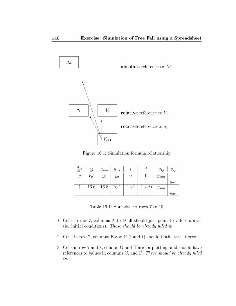
140 Exercise: Simulation of Free Fall using a Spreadsheet

∆t

ai Vi

Vi+1A

AA

AA

AK

relative reference to ai

6

relative reference to Vi

BB

BB

BB

BB

BB

BB

BB

BBM

absolute reference to ∆t

Figure 16.1: Simulation formula relationship

d2ydt2

dydt

ysim yact i t y1p y2p

g Vy0 y0 y0 0 0 ysim

yact

↑ 16.6 16.8 16.1 ↑ +1 ↑ +∆t ysim

yact

Table 16.1: Spreadsheet rows 7 to 10

1. Cells in row 7, columns A to D all should just point to values above;(ie. initial conditions). These should be already filled in.

2. Cells in row 7, columns E and F (i and t) should both start at zero.

3. Cells in row 7 and 8, column G and H are for plotting, and should havereferences to values in columns C, and D. These should be already filledin.

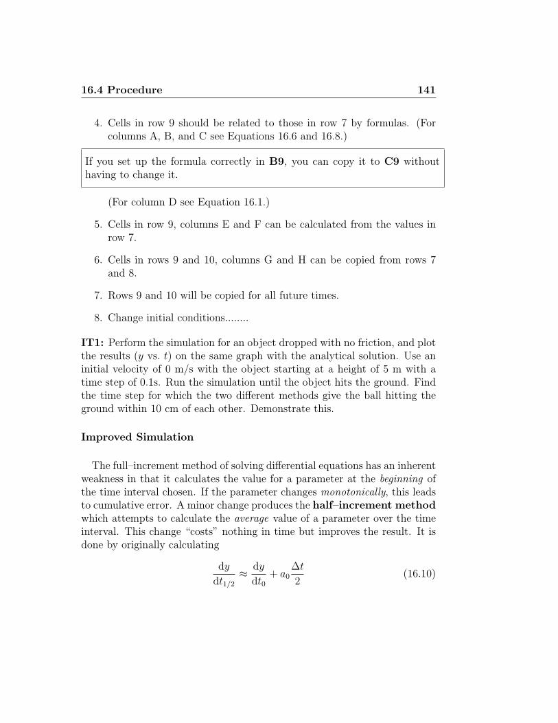
16.4 Procedure 141

4. Cells in row 9 should be related to those in row 7 by formulas. (Forcolumns A, B, and C see Equations 16.6 and 16.8.)

If you set up the formula correctly in B9, you can copy it to C9 withouthaving to change it.

(For column D see Equation 16.1.)

5. Cells in row 9, columns E and F can be calculated from the values inrow 7.

6. Cells in rows 9 and 10, columns G and H can be copied from rows 7and 8.

7. Rows 9 and 10 will be copied for all future times.

8. Change initial conditions........

IT1: Perform the simulation for an object dropped with no friction, and plotthe results (y vs. t) on the same graph with the analytical solution. Use aninitial velocity of 0 m/s with the object starting at a height of 5 m with atime step of 0.1s. Run the simulation until the object hits the ground. Findthe time step for which the two different methods give the ball hitting theground within 10 cm of each other. Demonstrate this.

Improved Simulation

The full–increment method of solving differential equations has an inherentweakness in that it calculates the value for a parameter at the beginning ofthe time interval chosen. If the parameter changes monotonically, this leadsto cumulative error. A minor change produces the half–increment methodwhich attempts to calculate the average value of a parameter over the timeinterval. This change “costs” nothing in time but improves the result. It isdone by originally calculating

dy

dt1/2

≈ dy

dt0+ a0

∆t

2(16.10)

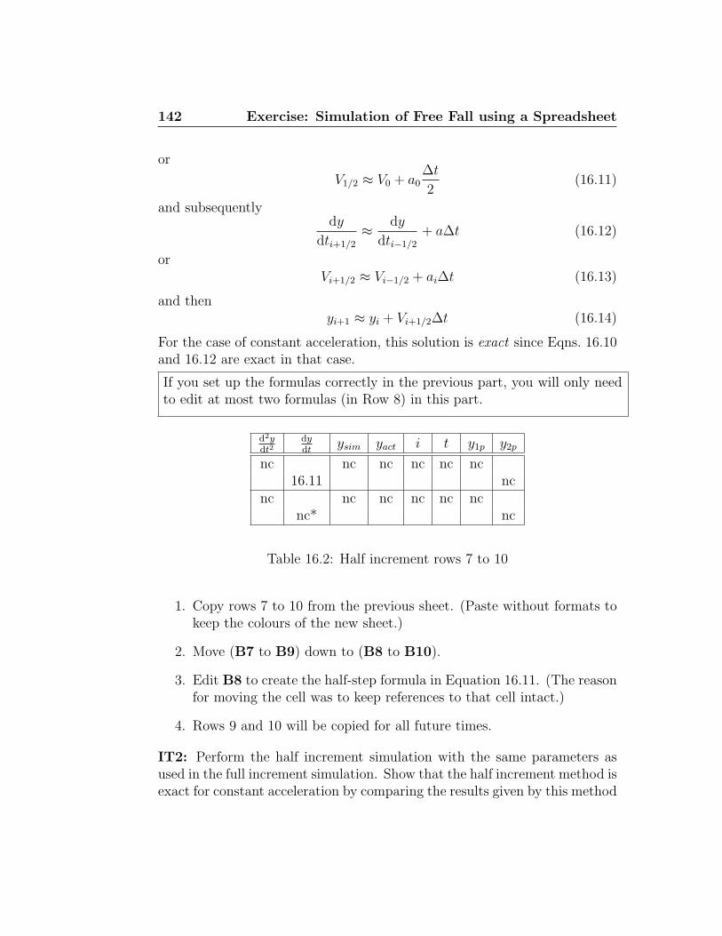
142 Exercise: Simulation of Free Fall using a Spreadsheet

or

V1/2 ≈ V0 + a0∆t

2(16.11)

and subsequentlydy

dti+1/2

≈ dy

dti−1/2

+ a∆t (16.12)

orVi+1/2 ≈ Vi−1/2 + ai∆t (16.13)

and thenyi+1 ≈ yi + Vi+1/2∆t (16.14)

For the case of constant acceleration, this solution is exact since Eqns. 16.10and 16.12 are exact in that case.

If you set up the formulas correctly in the previous part, you will only needto edit at most two formulas (in Row 8) in this part.

d2ydt2

dydt

ysim yact i t y1p y2p

nc nc nc nc nc nc16.11 nc

nc nc nc nc nc ncnc* nc

Table 16.2: Half increment rows 7 to 10

1. Copy rows 7 to 10 from the previous sheet. (Paste without formats tokeep the colours of the new sheet.)

2. Move (B7 to B9) down to (B8 to B10).

3. Edit B8 to create the half-step formula in Equation 16.11. (The reasonfor moving the cell was to keep references to that cell intact.)

4. Rows 9 and 10 will be copied for all future times.

IT2: Perform the half increment simulation with the same parameters asused in the full increment simulation. Show that the half increment method isexact for constant acceleration by comparing the results given by this method

16.4 Procedure 143

using a very large time step (0.1s) with the analytical solution. Demonstratethis.For the following exercises, use the half–increment method since it is moreaccurate than the full–increment method.

Adding Friction

A slightly more difficult (but more realistic) problem involves a frictionalforce acting on the ball due to air which is proportional to the square of thevelocity. For this problem, the frictional force is given by

|Ff | ∝ A |V |+ BV 2 (16.15)

and the force always acts to oppose the motion of the ball. Thus we canwrite the frictional force as

Ff = −(A + B |V |)V (16.16)

(This takes care of the sign of V .) To get the acceleration of the ball, we mustdivide the force acting on the ball by the mass of the ball, since F = ma.

• Now simulate this problem, plot y vs. t as before, and see how changingthe frictional force coefficients, A and B, changes the motion of the ball.(In this case, ay = g + afy = g − (A+B|V |)Vy

m.)

(Typical values for A and B for a ping pong ball are 5.9 × 10−6 and3.1× 10−4, respectively.)

If you set up the formulas correctly in the previous part, you will only needto edit two formulas (for the accelerations in Rows 7 and 9) in this part.

1. Copy rows 7 to 10 from the previous sheet. ( Paste without formats.)

2. Change A7 and A9 according to the equation for friction.

3. Rows 9 and 10 will be copied for all future times.

IT3: Perform the half increment simulation adding friction. How can yoube reasonably sure you have used a small enough time step for this last sim-ulation to give reasonable results, since you don’t have an analytical solutionto compare it with? Demonstrate this.

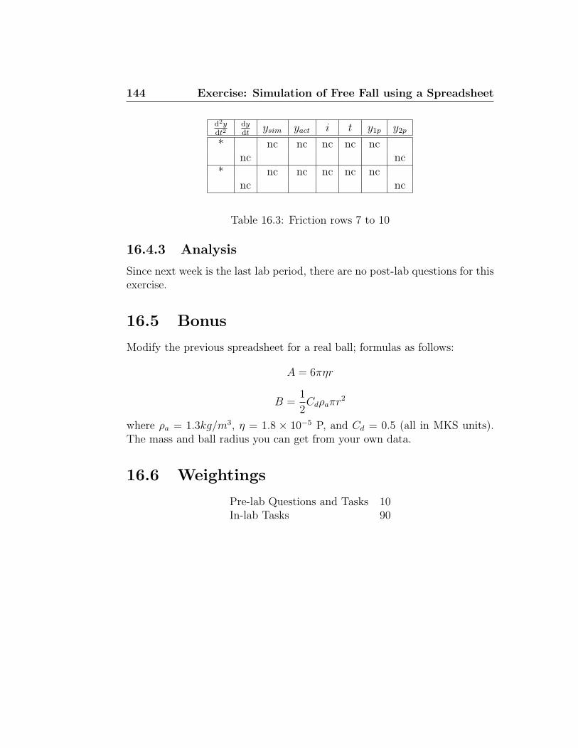
144 Exercise: Simulation of Free Fall using a Spreadsheet

d2ydt2

dydt

ysim yact i t y1p y2p

* nc nc nc nc ncnc nc

* nc nc nc nc ncnc nc

Table 16.3: Friction rows 7 to 10

16.4.3 Analysis

Since next week is the last lab period, there are no post-lab questions for thisexercise.

16.5 Bonus

Modify the previous spreadsheet for a real ball; formulas as follows:

A = 6πηr

B =1

2Cdρaπr2

where ρa = 1.3kg/m3, η = 1.8 × 10−5 P, and Cd = 0.5 (all in MKS units).The mass and ball radius you can get from your own data.

16.6 Weightings

Pre-lab Questions and Tasks 10In-lab Tasks 90

Chapter 17

Measuring “g”

17.1 Purpose

The purpose of this experiment is to measure the acceleration due to gravityand to see if the effects of air resistance can be observed by dropping variousballs and recording fall times.

17.2 Introduction

This experiment will introduce the concept of using uncertainties to comparenumbers.

Actually this experiment is really intended to illustrate the process you willgo through in each lab. The physics involved is extremely basic, so you shouldbe able to focus on how to analyze the results and prepare the report.

This lab will actually be broken into parts, so you will spend several weeksto produce the report. After you know how to do this, you will be able toproduce reports much more quickly.

The schedule will be somewhat like this:

• Evaluate uncertainties in raw data and collect data.

• Calculate uncertainties.

• Learn how to write up “Discussion of Uncertainties” and “Conclusions”in your report.

146 Measuring “g”

After that, you will hand in the lab. Note: the time for the parts men-tioned above may not all be consecutive; in research you often have severalprojects underway at once in different stages of completion.

17.3 Theory

17.3.1 Physics Behind This Experiment

For a body falling from rest under gravity, without air resistance, the heightfallen at time t will be given by

h =1

2gt2 (17.1)

17.3.2 About Experimentation in General

In order to learn anything useful from an experiment, it is critical to collectmeaningful data.

There are a few things to consider:

1. Data must be correct. (This means values must be recorded accurately,along with units.)

2. Data must be consistent. (Where you have repeated measurements,they should be similar.)

3. Data must be reproducible. (If you or someone else were to come backand do this later, the data should be similar to what you got the firsttime. This is more determined by your notes about what you do thanby the actual data.)

Collaboration

If you are working with a partner, it is important that you both understandahead of time what has to be done. It is easy to overlook details, but if twopeople are both thinking then it’s much less likely that something importantwill be missed.

Keep in mind that there may be some individual quantities which must beknown when doing an experiment which can change with time. If you do notrecord them at the time, you may have to redo the experiment completely.

17.3 Theory 147

Technique

How you collect the data may have a huge effect on the usefulness of thedata. Always consider alternatives which may be better.

Preliminary Calculations

Before you leave the lab you need to do preliminary calculations of importantresults to see if they are in the right ballpark. This should prevent youfrom making scale errors (such as using wrong units) and should avoid youforgetting to record time-sensitive values as mentioned above.

Well-Documented Raw Data

If your raw data are too messy or incomplete for you to understand later,you will have to redo the experiment. Always record

• Date

• Experimenters’ names and student ID numbers

• Lab section

• Experiment name

• For each type of measurement,

– Name of device used

– Precision measure

– Zero error (if applicable)

– Other factors in measurement making realistic uncertainty biggerthan the precision measure, and bound on uncertainty.

– Notes about how the measurement was taken or defined.

• For each table of data,

– Title

– Number

– Units for each column

148 Measuring “g”

– Uncertainties for each column; (If uncertainties change for datavalues in a column, make a column for the uncertainties.)

• For each question asked in the manual,

– Question number

– Answer

Most of the questions in this exercise are not numbered, but in labs they are.In the exercises, questions are often grouped together to try and develop a“big picture” of what is going on, and so the goal is to write explanationswhich address a group of questions, rather than handling each one individu-ally. This is the approach which you are to take in writing your “Discussionof Uncertainties” in a lab. Remember that wherever possible, you want toanswer questions from experiment, rather than from theory.

Uncertainties for all Measurements

Make sure that any value you record has an uncertainty. You should recordboth the precision measure of the instrument used, (if appropriate), and anyother factors which may make the actual uncertainty bigger than that andrationale for the size of the realistic uncertainty.

17.4 Procedure

17.4.1 Preparation

Most experiments and exercises will have requirements which must be com-pleted before the lab and presented at the beginning of the lab period.

Pre-lab Tasks

PT1: Look up the density of brass, steel, lead, aluminum, wood and cork.(If you find ambiguous information, explain.) Fill these values in Table 17.3,and record the reference for them.

17.4 Procedure 149

PT2: Rearrange Equation 17.1 to solve for g. In other words, complete thefollowing:

g =

Copy the result into Table 17.4.

PT3: Print off the “template” sheet of the spreadsheet for this experimentand bring it to the lab.

Pre-lab Questions

PQ1: If a person delays starting the watch after the ball is dropped, butdoes not delay stopping the watch when the ball hits the ground, what willbe the effect on the average time? What will be the effect on the value of gcalculated?

PQ2: If a person does not delay starting the watch when the ball is dropped,but delays stopping the watch after the ball hits the ground, what will bethe effect on the average time? What will be the effect on the value of gcalculated?

PQ3: If a person delays starting the watch after the ball is dropped and de-lays stopping the watch after the ball hits the ground, what will be the effecton the average time? What will be the effect on the value of g calculated?

17.4.2 Experimentation

Apparatus

• stopwatch

• bucket

• dense ball

• less dense ball

• tape measure

150 Measuring “g”

Method

Note about groups of 3: There is not really a difference between the rolesin a group of 3 and a group of two. For the purpose of the experiment,anyone who is not the “dropper” is the “gofer”; the important thing to noteis whether the person dropping the ball is the one timing it. Anyone notdropping the ball is functionally equivalent, regardless of which floor he orshe is on.

While you are getting the bucket lined up, practice drops with the pingpong ball. Once you have things aligned, you can switch to the dense ball.

1. Measure h.

2. Select a ball which you think should be relatively unaffected by frictionand time one drop. Repeat this a few times, to see how consistent yourtimes are.

3. Once you have some consistency in your times,do a calculation to seeif this gives you a reasonable result for g or not.

Note: This is not usually explicit in a lab, but you should always check whenyou collect data to see if your results are in the right ballpark, so you cancheck your data or repeat the experiment if there seems to be a problem. Ifyou wait until you are at home and find your results don’t make sense, andyour report is due the next day.....

4. Drop the ball several (ie. at least 5) times and record the fall times, asrecorded by both the dropper and the gofer. Calculate the average falltime.

5. Switch position, and repeat the previous steps.

6. Calculate values for g, based on the average times, Determine which ofthe methods gave the best result and try to figure out why. Note that“best” has to consider both accuracy and consistency of data.

7. Use the “preferred method” to collect data for a ball which shouldbe more affected by friction, by dropping the ball several times andrecording the fall times, as before.

8. Average the values for t and calculate g for the second type of ball.

17.4 Procedure 151

In-lab Tasks

IT1: For each instrument you use, copy the pertinent information into Ta-ble A.1 or Table A.2 of Appendix A.

IT2: Record at least experimental factors leading to uncertainty in h otherthan the one given and at least 2 experimental factors other than reactiontime leading to uncertainty in t Table 17.5 along with bounds and indicationof whether they are random, systematic, or possibly both.

IT3: Write up a Title and a Purpose for this experiment, which are moreappropriate than the ones given here. Be sure to include both quantitativegoals and qualitative ones in the “Purpose”. Hand these in.

In-lab Questions

Before leaving the lab, any determination of uncertainties in measurementsand other factors affecting uncertainties must be completed. After you leavethe lab, you may never see the equipment set up the same way again!

IQ1: What is the realistic uncertainty in h, and what experimental factor(s)cause it? This value should be one you feel you can defend as being neitherextremely high nor extremely low. (There may be more than one contributingfactor.)

IQ2: Was the technique which produced the most accurate time also theone which produced the most precise (ie. consistent) time? How difficult isit to determine the “best” technique if the most accurate one is not the mostprecise one?

17.4.3 Analysis

Before learning how to analyze uncertainties, there may be few obvious con-clusions to be drawn from an experiment. The following steps will be com-pleted in later exercises.

1. Calculate the standard deviation and standard deviation of the meanfor the sets of times for each of the types of ball, and then determinethe uncertainty in t̄ for each data set.

2. Determine the formula for the uncertainty in g, given the uncertaintiesin h and t̄.

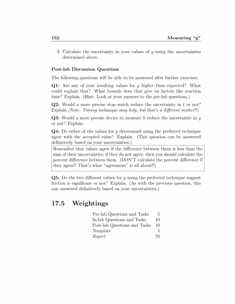
152 Measuring “g”

3. Calculate the uncertainty in your values of g using the uncertaintiesdetermined above.

Post-lab Discussion Questions

The following questions will be able to be answered after further exercises.

Q1: Are any of your resulting values for g higher than expected? Whatcould explain that? What bounds does that give on factors like reactiontime? Explain. (Hint: Look at your answers to the pre-lab questions.)

Q2: Would a more precise stop watch reduce the uncertainty in t or not?Explain.(Note: Timing technique may help, but that’s a different matter!!)

Q3: Would a more precise device to measure h reduce the uncertainty in gor not? Explain.

Q4: Do either of the values for g determined using the preferred techniqueagree with the accepted value? Explain. (This question can be answereddefinitively based on your uncertainties.)

Remember that values agree if the difference between them is less than thesum of their uncertainties; if they do not agree, then you should calculate thepercent difference between them. (DON’T calculate the percent difference ifthey agree!! That’s what “agreement” is all about!!)

Q5: Do the two different values for g using the preferred technique suggestfriction is significant or not? Explain. (As with the previous question, thiscan answered definitively based on your uncertainties.)

17.5 Weightings

Pre-lab Questions and Tasks 5In-lab Questions and Tasks 10Post-lab Questions and Tasks 10Template 5Report 70

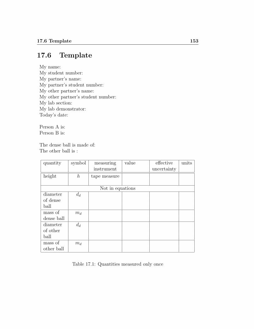
17.6 Template 153

17.6 Template

My name:My student number:My partner’s name:My partner’s student number:My other partner’s name:My other partner’s student number:My lab section:My lab demonstrator:Today’s date:

Person A is:Person B is:

The dense ball is made of:The other ball is :

quantity symbol measuring value effective unitsinstrument uncertainty

height h tape measure

Not in equationsdiameter dd

of denseballmass of md

dense balldiameter dd

of otherballmass of md

other ball

Table 17.1: Quantities measured only once

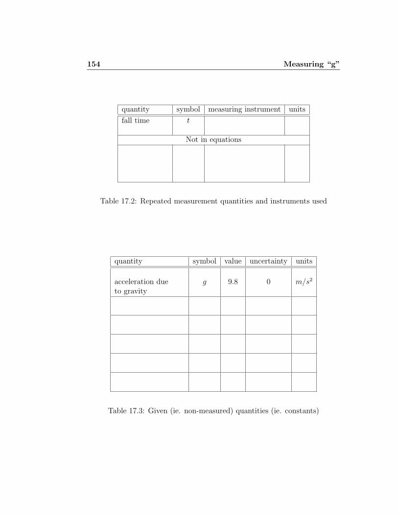
154 Measuring “g”

quantity symbol measuring instrument units

fall time t

Not in equations

Table 17.2: Repeated measurement quantities and instruments used

quantity symbol value uncertainty units

acceleration due g 9.8 0 m/s2

to gravity

Table 17.3: Given (ie. non-measured) quantities (ie. constants)

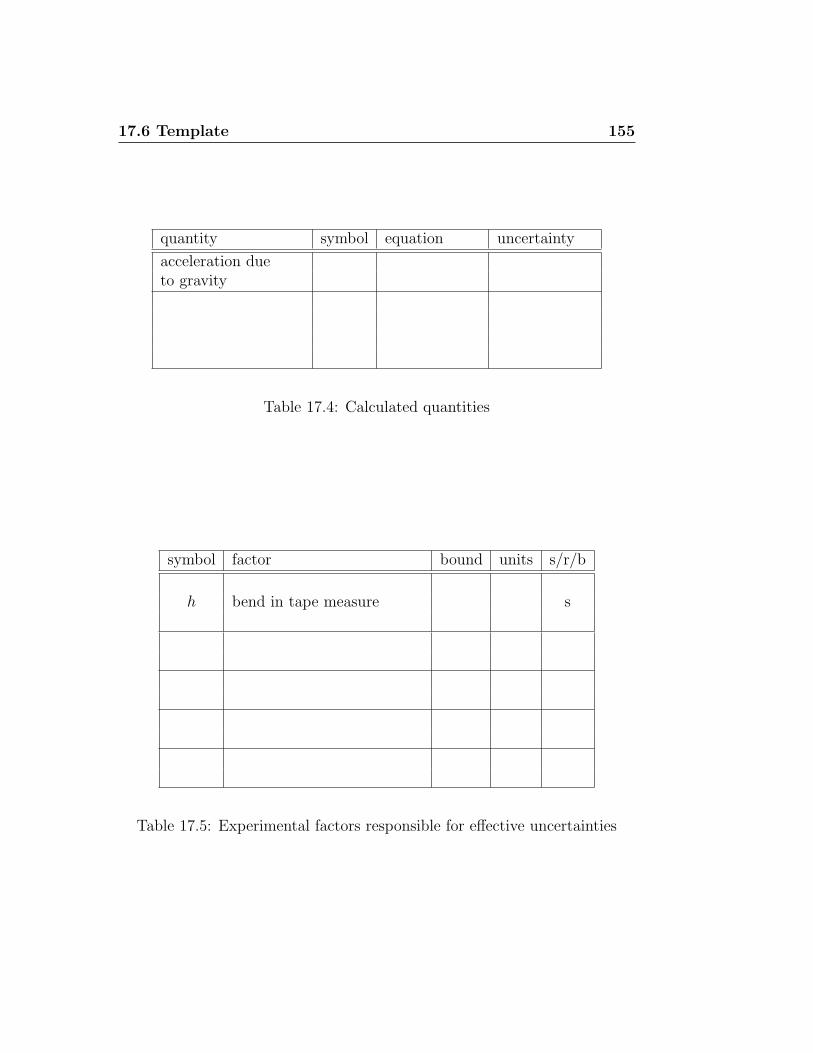
17.6 Template 155

quantity symbol equation uncertainty

acceleration dueto gravity

Table 17.4: Calculated quantities

symbol factor bound units s/r/b

h bend in tape measure s

Table 17.5: Experimental factors responsible for effective uncertainties

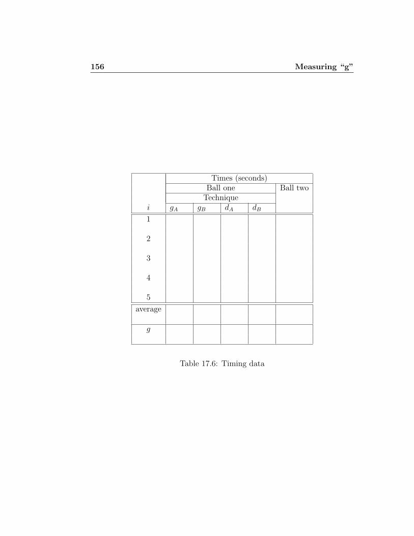
156 Measuring “g”

Times (seconds)Ball one Ball two

Techniquei gA gB dA dB

1

2

3

4

5

average

g

Table 17.6: Timing data

Chapter 18

Moment of Inertia

18.1 Purpose

The purpose of this experiment is to determine empirically the moment ofinertia of a body about an axis and to compare this with the theoreticalvalue calculated from the measured mass and dimensions of the body. Thisexperiment will also examine what factors affect an object rolling down anincline.

18.2 Introduction

This experiment tests basic calculations with uncertainties and repeated inde-pendent measurements. In this experiment, there are several places involvingthe choice of certain parameters. How these choices affect the uncertaintiesinvolved is important.

18.3 Theory

Understanding rotational motion is a lot easier if you realize that the quanti-ties involved are analogous to the familiar quantities in linear motion, and theresulting equations are analogous. The following two tables should illustratethis.

Some of the equations relating the quantities are shown below.

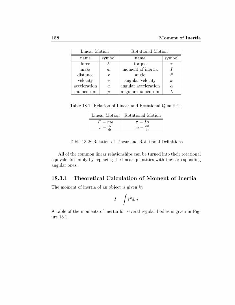
158 Moment of Inertia

Linear Motion Rotational Motion

name symbol name symbolforce F torque τmass m moment of inertia I

distance x angle θvelocity v angular velocity ω

acceleration a angular acceleration αmomentum p angular momentum L

Table 18.1: Relation of Linear and Rotational Quantities

Linear Motion Rotational Motion

F = ma τ = Iαv = dx

dtω = dθ

dt

Table 18.2: Relation of Linear and Rotational Definitions

All of the common linear relationships can be turned into their rotationalequivalents simply by replacing the linear quantities with the correspondingangular ones.

18.3.1 Theoretical Calculation of Moment of Inertia

The moment of inertia of an object is given by

I =

∫r2dm

A table of the moments of inertia for several regular bodies is given in Fig-ure 18.1.

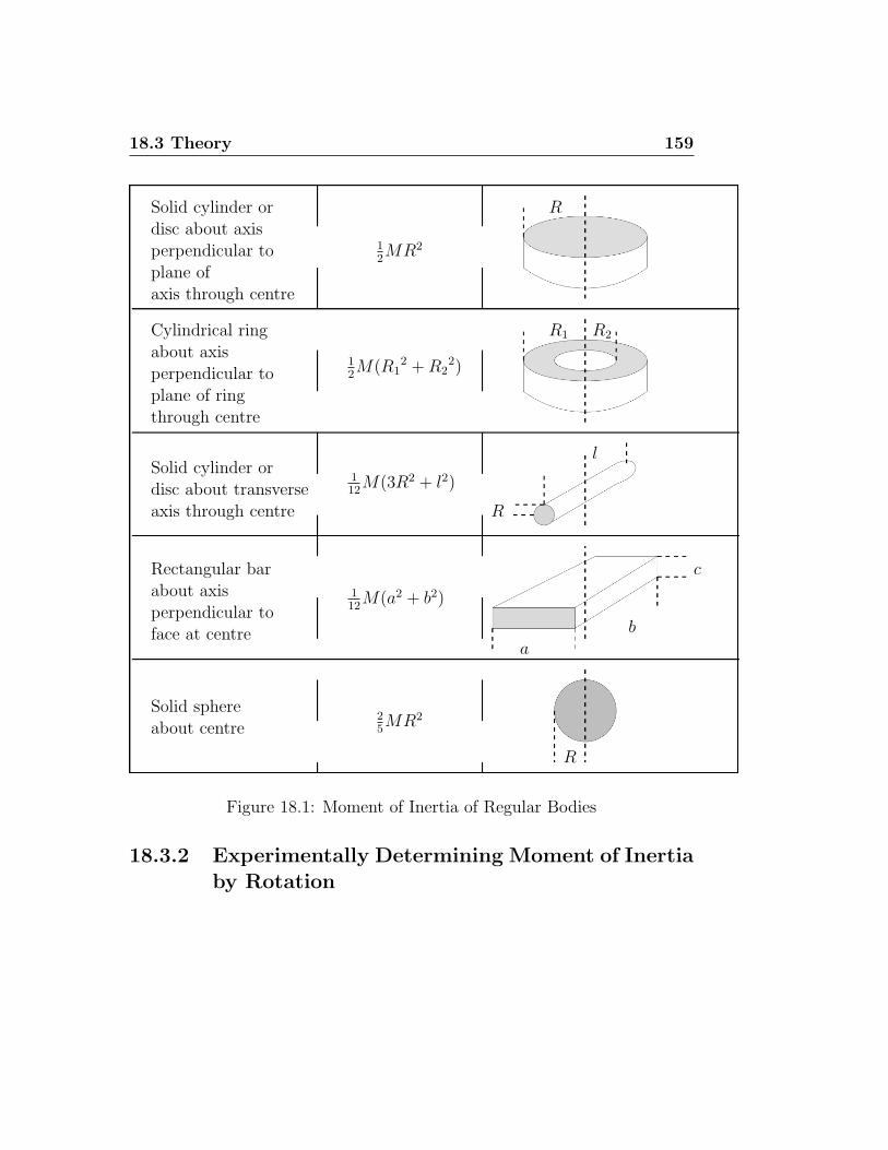
18.3 Theory 159

12MR2

12M(R1

2 + R22)

112

M(3R2 + l2)

112

M(a2 + b2)

25MR2

R

R1 R2

l

R

c

ba

R

Solid cylinder ordisc about axisperpendicular toplane ofaxis through centre

Cylindrical ringabout axisperpendicular toplane of ringthrough centre

Solid cylinder ordisc about transverseaxis through centre

Rectangular barabout axisperpendicular toface at centre

Solid sphereabout centre

Figure 18.1: Moment of Inertia of Regular Bodies

18.3.2 Experimentally Determining Moment of Inertiaby Rotation

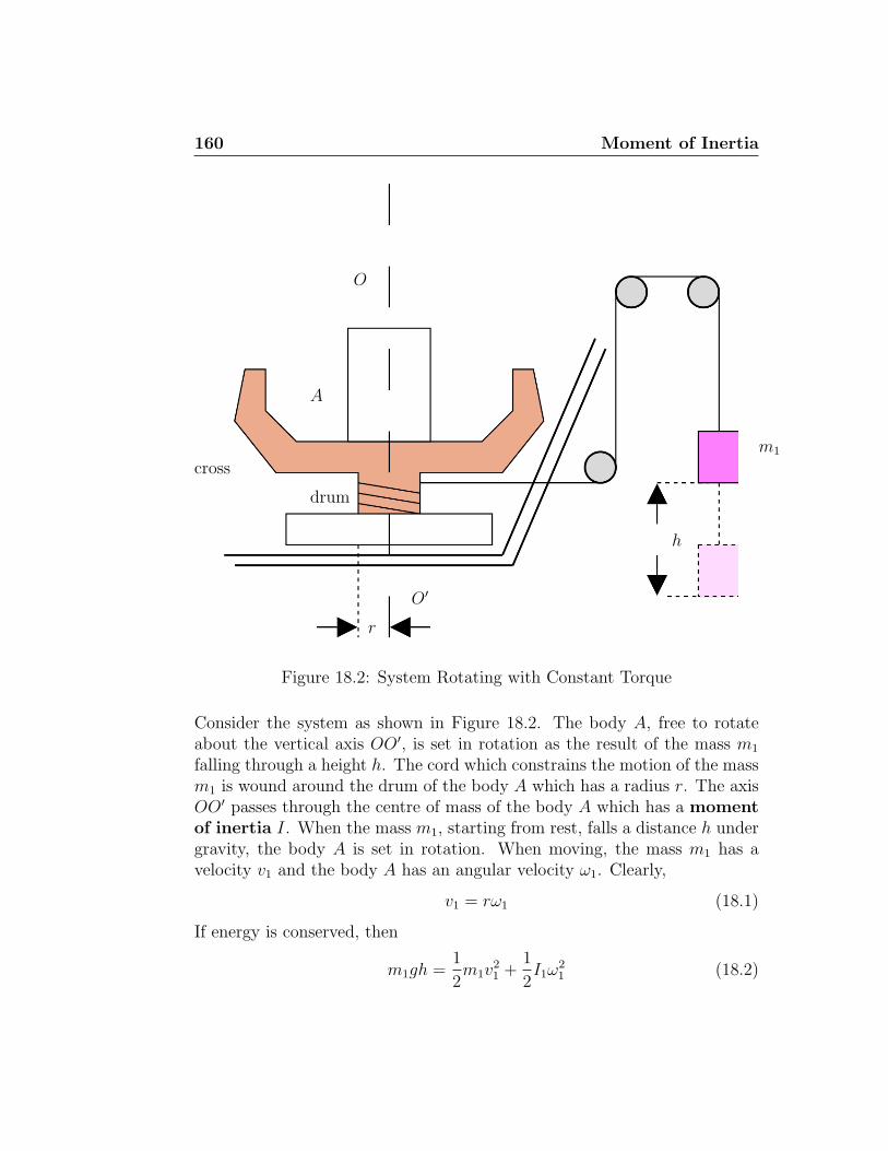
160 Moment of Inertia

A

O

O′

cross

drum

r

m1

h

Figure 18.2: System Rotating with Constant Torque

Consider the system as shown in Figure 18.2. The body A, free to rotateabout the vertical axis OO′, is set in rotation as the result of the mass m1

falling through a height h. The cord which constrains the motion of the massm1 is wound around the drum of the body A which has a radius r. The axisOO′ passes through the centre of mass of the body A which has a momentof inertia I. When the mass m1, starting from rest, falls a distance h undergravity, the body A is set in rotation. When moving, the mass m1 has avelocity v1 and the body A has an angular velocity ω1. Clearly,

v1 = rω1 (18.1)

If energy is conserved, then

m1gh =1

2m1v

21 +

1

2I1ω

21 (18.2)

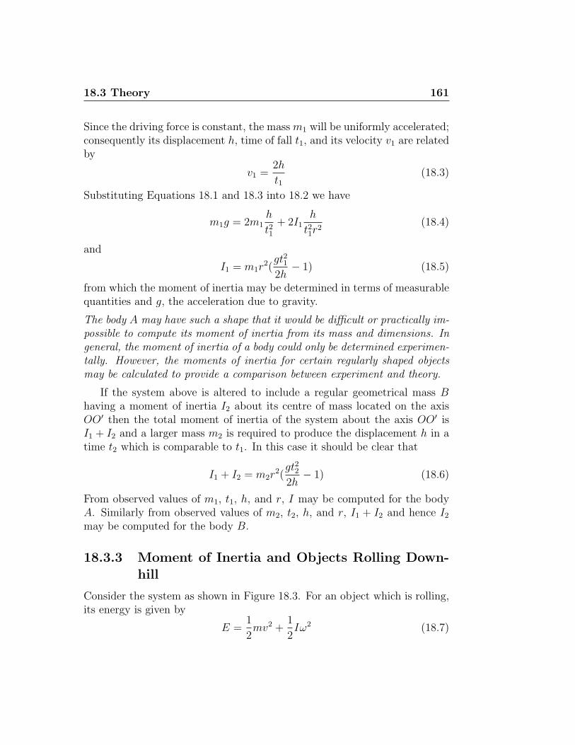
18.3 Theory 161

Since the driving force is constant, the mass m1 will be uniformly accelerated;consequently its displacement h, time of fall t1, and its velocity v1 are relatedby

v1 =2h

t1(18.3)

Substituting Equations 18.1 and 18.3 into 18.2 we have

m1g = 2m1h

t21+ 2I1

h

t21r2

(18.4)

and

I1 = m1r2(

gt212h

− 1) (18.5)

from which the moment of inertia may be determined in terms of measurablequantities and g, the acceleration due to gravity.

The body A may have such a shape that it would be difficult or practically im-possible to compute its moment of inertia from its mass and dimensions. Ingeneral, the moment of inertia of a body could only be determined experimen-tally. However, the moments of inertia for certain regularly shaped objectsmay be calculated to provide a comparison between experiment and theory.

If the system above is altered to include a regular geometrical mass Bhaving a moment of inertia I2 about its centre of mass located on the axisOO′ then the total moment of inertia of the system about the axis OO′ isI1 + I2 and a larger mass m2 is required to produce the displacement h in atime t2 which is comparable to t1. In this case it should be clear that

I1 + I2 = m2r2(

gt222h

− 1) (18.6)

From observed values of m1, t1, h, and r, I may be computed for the bodyA. Similarly from observed values of m2, t2, h, and r, I1 + I2 and hence I2

may be computed for the body B.

18.3.3 Moment of Inertia and Objects Rolling Down-hill

Consider the system as shown in Figure 18.3. For an object which is rolling,its energy is given by

E =1

2mv2 +

1

2Iω2 (18.7)

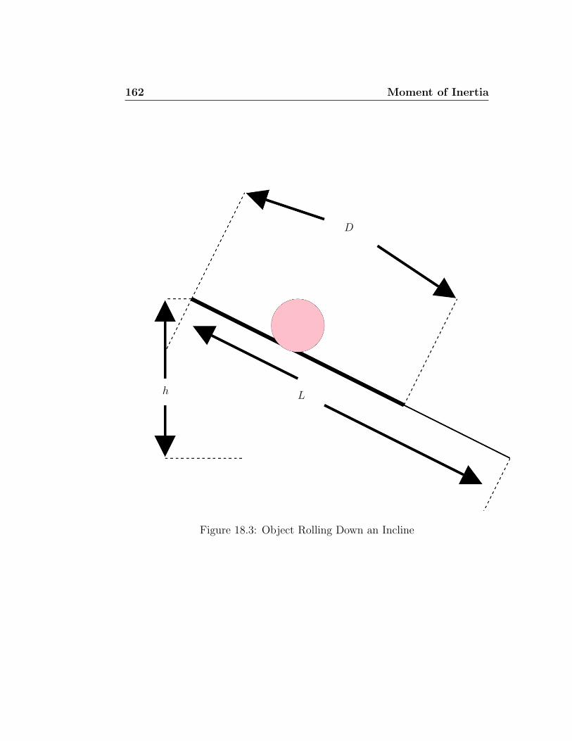
162 Moment of Inertia

D

Lh

Figure 18.3: Object Rolling Down an Incline

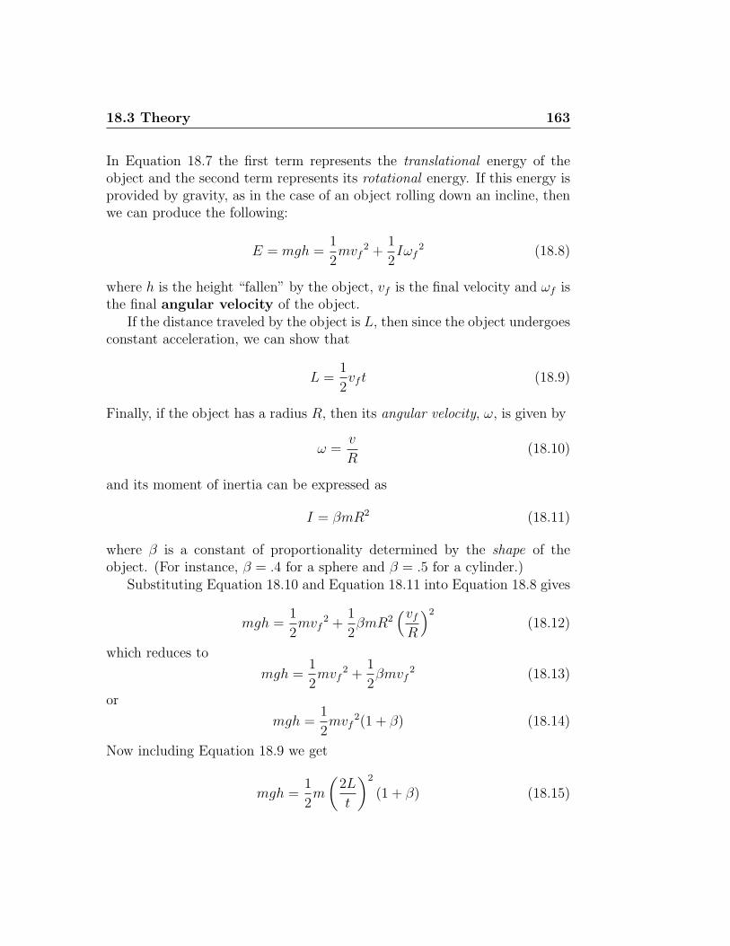
18.3 Theory 163

In Equation 18.7 the first term represents the translational energy of theobject and the second term represents its rotational energy. If this energy isprovided by gravity, as in the case of an object rolling down an incline, thenwe can produce the following:

E = mgh =1

2mvf

2 +1

2Iωf

2 (18.8)

where h is the height “fallen” by the object, vf is the final velocity and ωf isthe final angular velocity of the object.

If the distance traveled by the object is L, then since the object undergoesconstant acceleration, we can show that

L =1

2vf t (18.9)

Finally, if the object has a radius R, then its angular velocity, ω, is given by

ω =v

R(18.10)

and its moment of inertia can be expressed as

I = βmR2 (18.11)

where β is a constant of proportionality determined by the shape of theobject. (For instance, β = .4 for a sphere and β = .5 for a cylinder.)

Substituting Equation 18.10 and Equation 18.11 into Equation 18.8 gives

mgh =1

2mvf

2 +1

2βmR2

(vf

R

)2

(18.12)

which reduces to

mgh =1

2mvf

2 +1

2βmvf

2 (18.13)

or

mgh =1

2mvf

2(1 + β) (18.14)

Now including Equation 18.9 we get

mgh =1

2m

(2L

t

)2

(1 + β) (18.15)

164 Moment of Inertia

from which we get

1 + β =2mgh

m(

2Lt

)2 (18.16)

and finally

β =ght2

2L2− 1 (18.17)

You will notice that in the above equation, only h, t, and L are left; i.e. onlythe shape of the object matters, not the size or the mass. Note the similarityin form to the term in parentheses in Equation 18.5.

If you are only using part of the ramp, then Equation 18.17 becomes

β =ght2

2DL− 1 (18.18)

where D is the distance used.

18.4 Procedure

18.4.1 Preparation

Pre-lab Questions

PQ1: Does your experience in the Measuring ‘g’ lab give you any insightsinto how to do the best timing? Explain. (Hint: think about the two rolesinvolved in that experiment, and which role produced better timing.)

PQ2: Based on Equation 18.11, what is β for a sphere? For a cylinder?What would it be for a very thin hoop (where the inner and outer radii areessentially equal)?

PQ3: Based on Equation 18.17, will an object roll faster if β is smaller orlarger? Which will roll slower; a sphere or a cylinder?

Pre-lab Tasks

PT1: Copy the equation you determined for ∆I for a ring in the “ProcessingUncertainties” exercise into Table 18.6.

18.4 Procedure 165

PT2: From Equation 18.5, determine ∆I1 given m1, ∆m1, r, ∆r, etc. Copythis into Table 18.6.

PT3: From Figure 18.1, determine ∆I for a cylinder given M , ∆M , R and∆R. Rewrite the expression for ∆I for the situation where it is the diameter,D, and its uncertainty ∆D which is measured instead of the radius. Copythis into Table 18.6.

PT4: From Equation 18.18, determine ∆β given D, ∆D, t, ∆t, etc. Copythis into Table 18.6.

18.4.2 Experimentation

Apparatus

The apparatus consists of a light metal cross mounted on ball bearings so asto rotate in a horizontal plane about a vertical axis, as shown in Figure 18.2.The cross serves as a carrier for the object whose moment of inertia is tobe determined. The drum is driven by means of a falling weight connectedto the drum by means of a cord wrapped around the drum and a couple ofpulleys. The bodies whose moments of inertia are to be determined are aring, a disc, and a cylinder.

In-lab Tasks

In this experiment, the in-lab tasks are included with each part.

In-lab Questions

In this experiment, the in-lab questions are included with each part.

Method

Part 1: Moment of Inertia of the Cross and Drum

Since the cross and drum combination has a complex shape, it would bedifficult to determine its moment of inertia theoretically. Following is theprocess to determine it experimentally.

1. With the vernier caliper measure the diameter 2r of the drum.

166 Moment of Inertia

2. Take a cord about 4 metres long and after passing it over the top pulleyand under the bottom one wind a little more than a metre of it on thedrum. Adjust until the possible distance of the fall is about one metre.

3. Make a loop in the free end of the cord and in this loop insert smallriders1, 1/2 to 1 g each, one at a time until the cross rotates withconstant speed when started. This mass will serve (it is hoped!) tocancel out the effect of friction on your results. Since these masses aresmall in comparison with the accelerated mass, their effect on valuesobtained from Equation 18.5 and Equation 18.6 is negligible. Of coursethe mass of the riders should not be included as part of m in theseequations.

4. Now attach an additional mass m1 to this cord. This mass is the bodywhose weight furnishes the driving force. Select and accurately measurethe distance of fall h and make several determinations of the time offall t1 through this distance. Use these to fill in Table 18.8.

IQ1: To get the best value for I, is the ideal choice for m1 a large or a smallmass? Why? (ie. Consider how the choice of either a very large or a verysmall mass would affect the experiment.)

IQ2: What is the realistic uncertainty in h and what causes it? How repro-duceable is h? (ie. How easy is it to ensure that two different objects aredropped the same distance?)

IQ3: How much uncertainty in m1 is due to trying to determine constantvelocity for the system?

IQ4: How does the mass of the individual riders affect the uncertainty inm1?

IT1: Do an order of magnitude calculation for I.

Part 2: Moments of Inertia of Regularly Shaped Objects

Experimental Determination

Note that for the experimental determination of I, M and R don’t matter!

1Paper clips work well for this.

18.4 Procedure 167

1. Place one of the regularly shaped objects on the metal cross so that itscentre of mass is on the axis of rotation.

2. Add appropriate riders until the system rotates at a constant speed.As before, the mass of these riders may be neglected in computing themoment of inertia.

3. Now add a mass m2 to the string in place of m1 and observe time offall t2 over the distance h. The mass m2 should be much larger sincethe moment of inertia of the cross, drum, and object is much largerthan the moment of inertia of the cross and drum alone.

4. Repeat this several times as in Part 1 and fill in Table 18.9.

5. Repeat the above measurements placing one other regularly shapedobject on the cross and fill in Table 18.10.

IQ5: As in Part 1, is the ideal choice for m2 a large or a small mass? Why?(ie. Consider how the choice of either a very large or a very small mass wouldaffect the experiment.) How should it compare to m1?

IQ6: Consider the questions in IQ3 and IQ4 above with m1 replaced by m2.In other words, in the uncertainty in m2 similar to the uncertainty in m1?Explain.

IT2: Do an order of magnitude calculation of I for each object.

Theoretical Determination

Note that for the theoretical determination of I, m1, m2, r, etc. don’t matter!

1. Determine the linear dimensions and the masses of the regularly shapedobjects whose moments of inertia are to be determined. (Measure di-ameter instead of radius to avoid having to determine where the centreis.)

IT3: Do an order of magnitude calculation for I for each object, and seethat they are similar to values given previously.

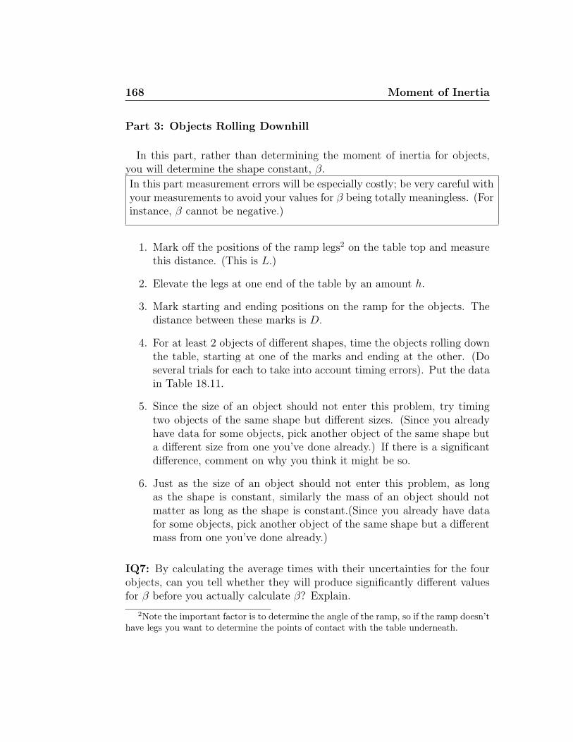
168 Moment of Inertia

Part 3: Objects Rolling Downhill

In this part, rather than determining the moment of inertia for objects,you will determine the shape constant, β.

In this part measurement errors will be especially costly; be very careful withyour measurements to avoid your values for β being totally meaningless. (Forinstance, β cannot be negative.)

1. Mark off the positions of the ramp legs2 on the table top and measurethis distance. (This is L.)

2. Elevate the legs at one end of the table by an amount h.

3. Mark starting and ending positions on the ramp for the objects. Thedistance between these marks is D.

4. For at least 2 objects of different shapes, time the objects rolling downthe table, starting at one of the marks and ending at the other. (Doseveral trials for each to take into account timing errors). Put the datain Table 18.11.

5. Since the size of an object should not enter this problem, try timingtwo objects of the same shape but different sizes. (Since you alreadyhave data for some objects, pick another object of the same shape buta different size from one you’ve done already.) If there is a significantdifference, comment on why you think it might be so.

6. Just as the size of an object should not enter this problem, as longas the shape is constant, similarly the mass of an object should notmatter as long as the shape is constant.(Since you already have datafor some objects, pick another object of the same shape but a differentmass from one you’ve done already.)

IQ7: By calculating the average times with their uncertainties for the fourobjects, can you tell whether they will produce significantly different valuesfor β before you actually calculate β? Explain.

2Note the important factor is to determine the angle of the ramp, so if the ramp doesn’thave legs you want to determine the points of contact with the table underneath.

18.4 Procedure 169

IQ8: What is the smallest value for h which can be measured reasonablyprecisely (say, with ∆h . 0.1h)? What is the smallest value for t which canbe measured reasonably precisely (say, with ∆t . 0.1t)? What do these twosuggest about what angles ought to be used to determine β? (Hint: How areheight and time related?) Explain.

IQ9: How can you set up the experiment so that the size of the object useddoes not affect your measurement of the distance D or its uncertainty?

IT4: Do an order of magnitude calculation for β for each object, and seethat they are in the correct range.

18.4.3 Analysis

Note that you have two different radii to work with; r, the radius of thedrum, and R, the radius of the ring, disc, etc. Do not get these confused!

Part 1: Moment of Inertia of the Cross and Drum

Using the data in Table 18.8, calculate the average value of t1 and itsuncertainty. Use this to calculate I1 and its uncertainty for the cross anddrum combination.

Part 2: Moments of Inertia of Regularly Shaped Objects

Experimental Determination

1. Using the data in Table 18.9, compute the moment of inertia I1 + I2 ofthe cross, drum, and the regularly shaped object and its uncertainty.

2. Subtract the value of I1 from the value for I1 + I2 in order to get themoment of inertia for the regularly shaped object and its uncertainty.

3. Repeat the previous two steps for the data for the other object inTable 18.10.

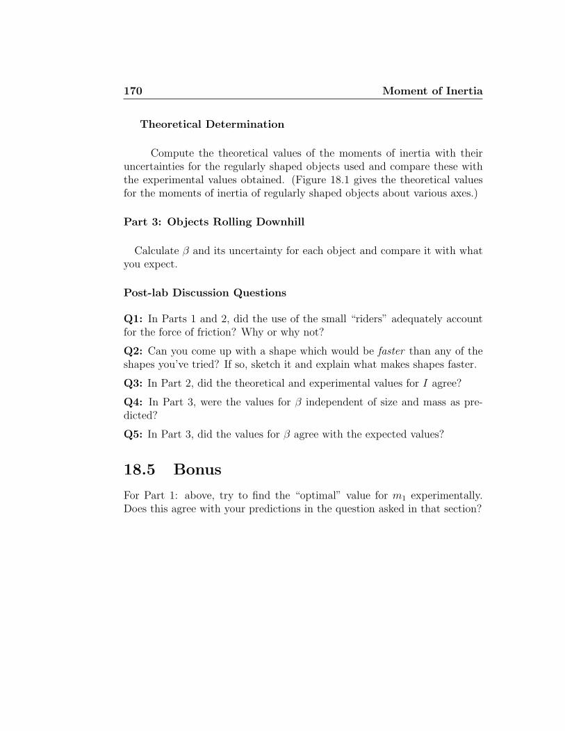
170 Moment of Inertia

Theoretical Determination

Compute the theoretical values of the moments of inertia with theiruncertainties for the regularly shaped objects used and compare these withthe experimental values obtained. (Figure 18.1 gives the theoretical valuesfor the moments of inertia of regularly shaped objects about various axes.)

Part 3: Objects Rolling Downhill

Calculate β and its uncertainty for each object and compare it with whatyou expect.

Post-lab Discussion Questions

Q1: In Parts 1 and 2, did the use of the small “riders” adequately accountfor the force of friction? Why or why not?

Q2: Can you come up with a shape which would be faster than any of theshapes you’ve tried? If so, sketch it and explain what makes shapes faster.

Q3: In Part 2, did the theoretical and experimental values for I agree?

Q4: In Part 3, were the values for β independent of size and mass as pre-dicted?

Q5: In Part 3, did the values for β agree with the expected values?

18.5 Bonus

For Part 1: above, try to find the “optimal” value for m1 experimentally.Does this agree with your predictions in the question asked in that section?

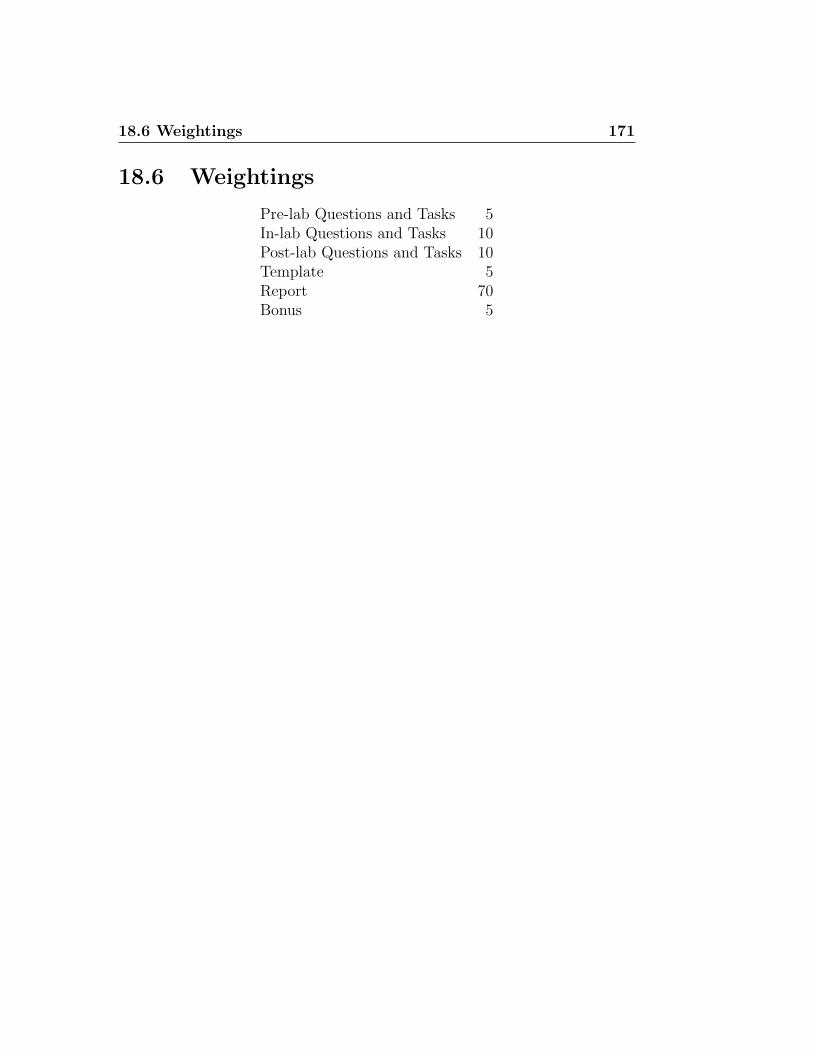
18.6 Weightings 171

18.6 Weightings

Pre-lab Questions and Tasks 5In-lab Questions and Tasks 10Post-lab Questions and Tasks 10Template 5Report 70Bonus 5

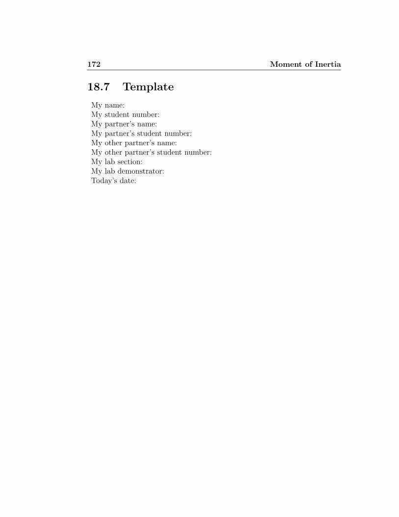
172 Moment of Inertia

18.7 Template

My name:My student number:My partner’s name:My partner’s student number:My other partner’s name:My other partner’s student number:My lab section:My lab demonstrator:Today’s date:

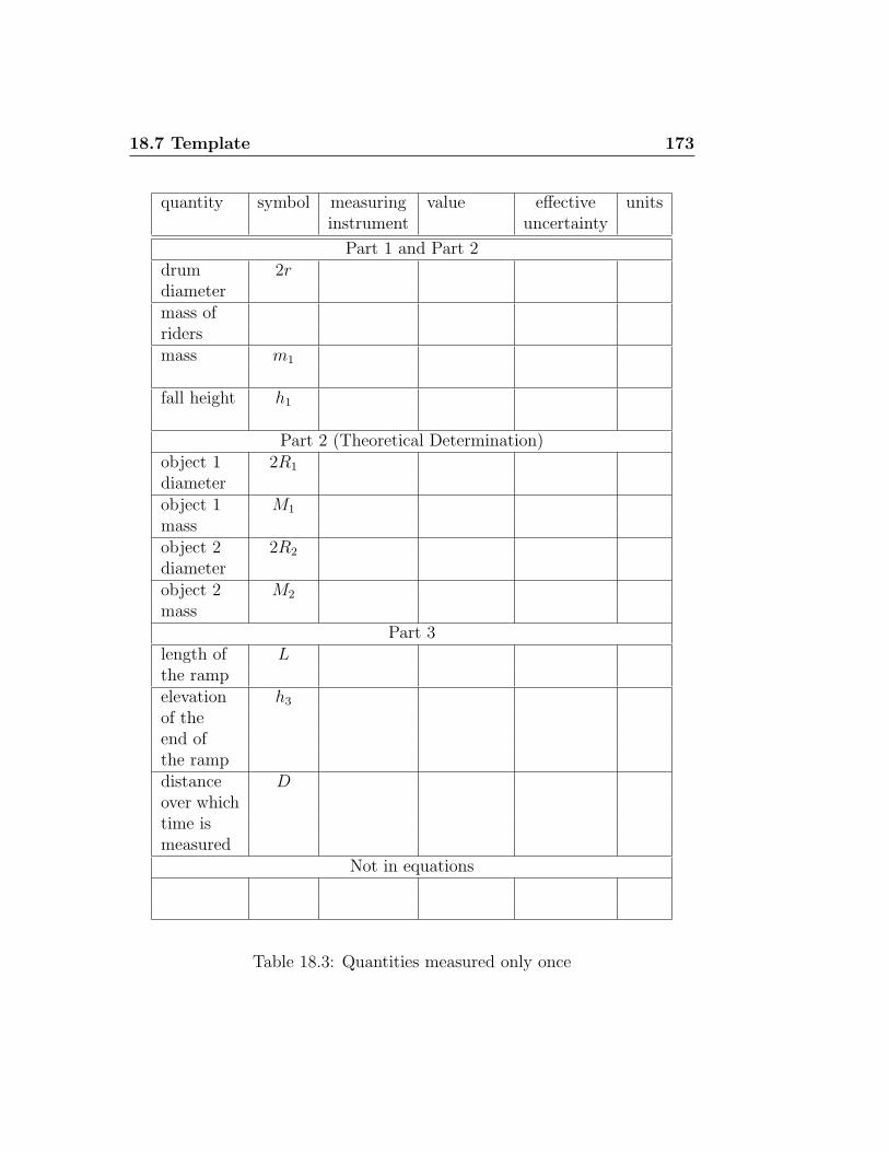
18.7 Template 173

quantity symbol measuring value effective unitsinstrument uncertainty

Part 1 and Part 2drum 2rdiametermass ofridersmass m1

fall height h1

Part 2 (Theoretical Determination)object 1 2R1

diameterobject 1 M1

massobject 2 2R2

diameterobject 2 M2

massPart 3

length of Lthe rampelevation h3

of theend ofthe rampdistance Dover whichtime ismeasured

Not in equations

Table 18.3: Quantities measured only once

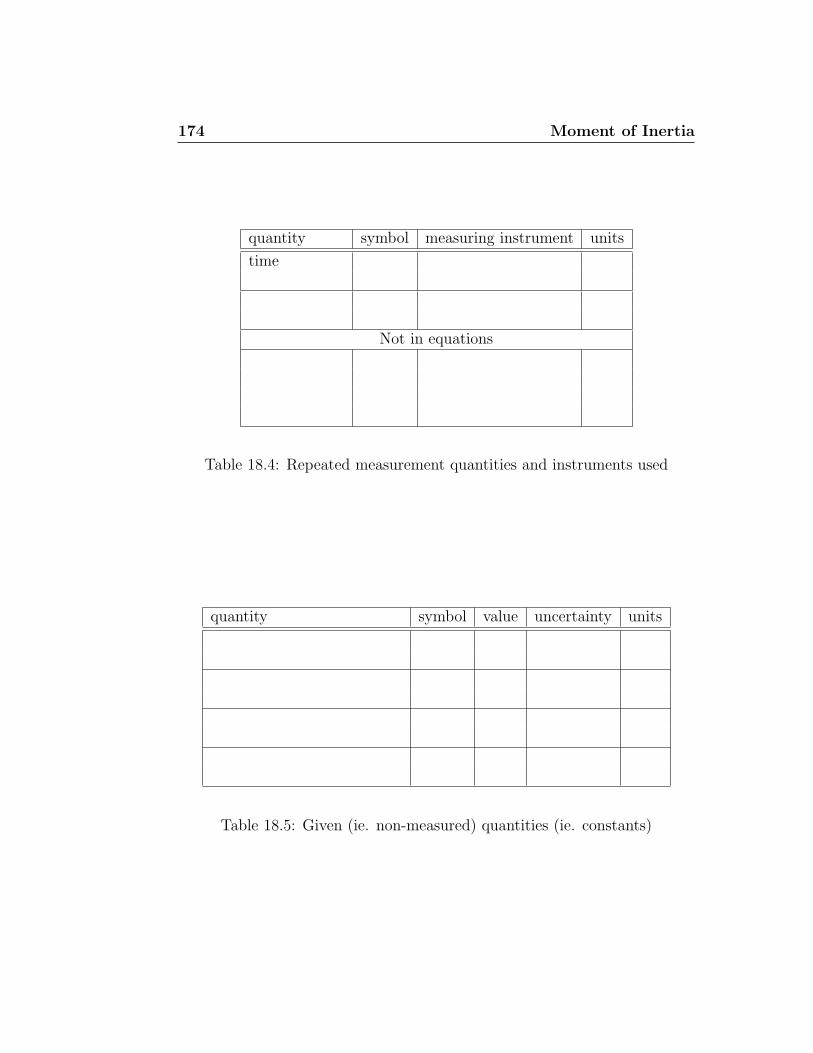
174 Moment of Inertia

quantity symbol measuring instrument units

time

Not in equations

Table 18.4: Repeated measurement quantities and instruments used

quantity symbol value uncertainty units

Table 18.5: Given (ie. non-measured) quantities (ie. constants)

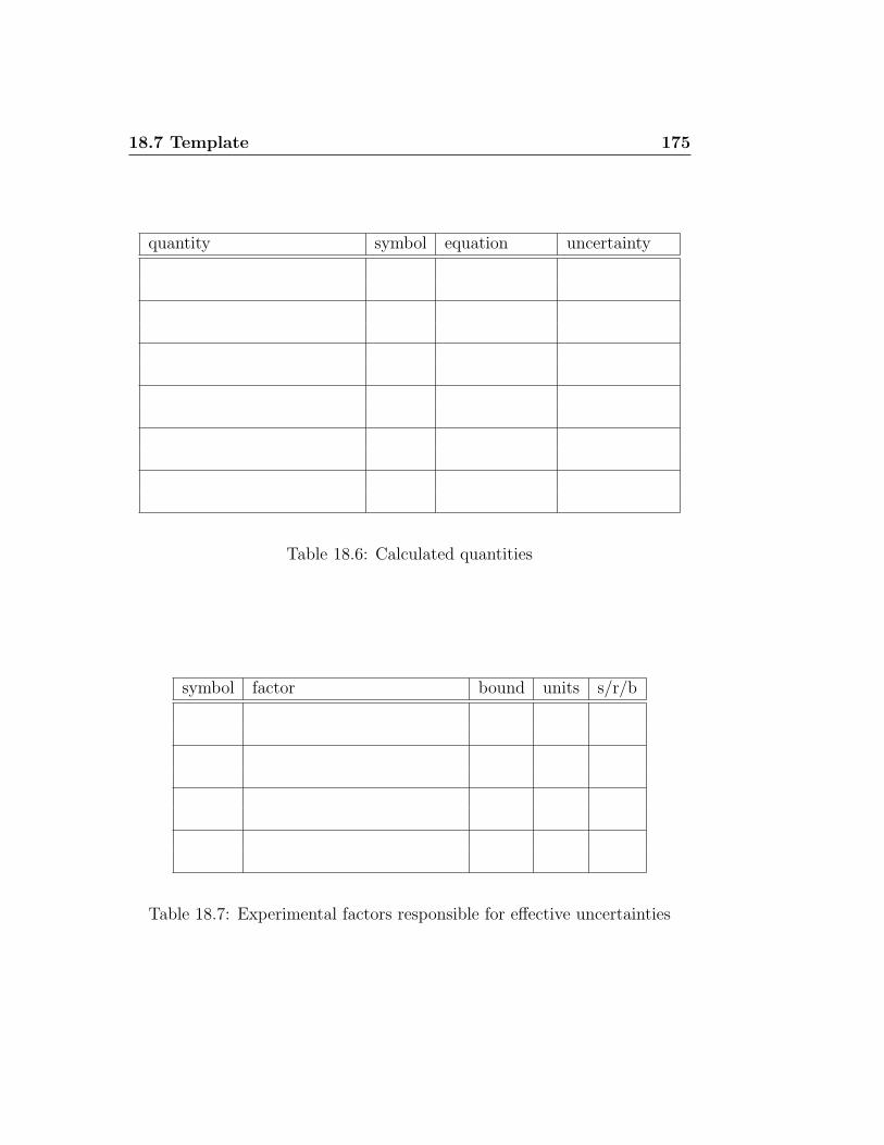
18.7 Template 175

quantity symbol equation uncertainty

Table 18.6: Calculated quantities

symbol factor bound units s/r/b

Table 18.7: Experimental factors responsible for effective uncertainties

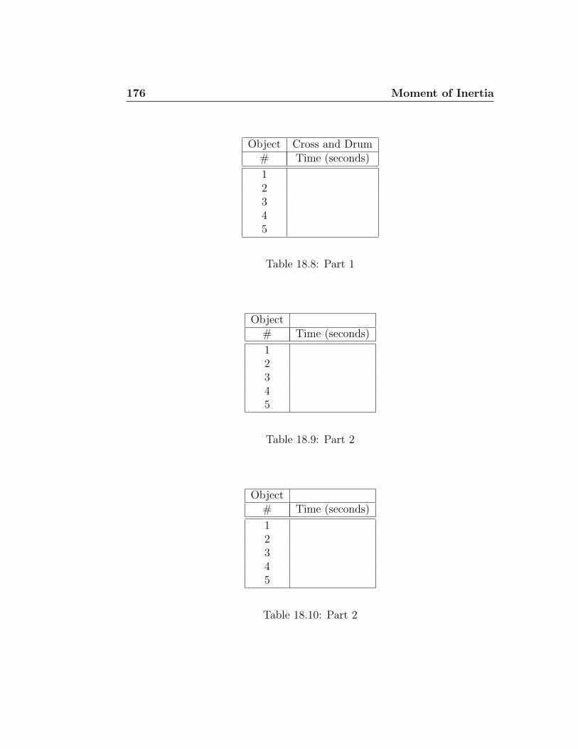
176 Moment of Inertia

Object Cross and Drum# Time (seconds)

12345

Table 18.8: Part 1

Object# Time (seconds)

12345

Table 18.9: Part 2

Object# Time (seconds)

12345

Table 18.10: Part 2

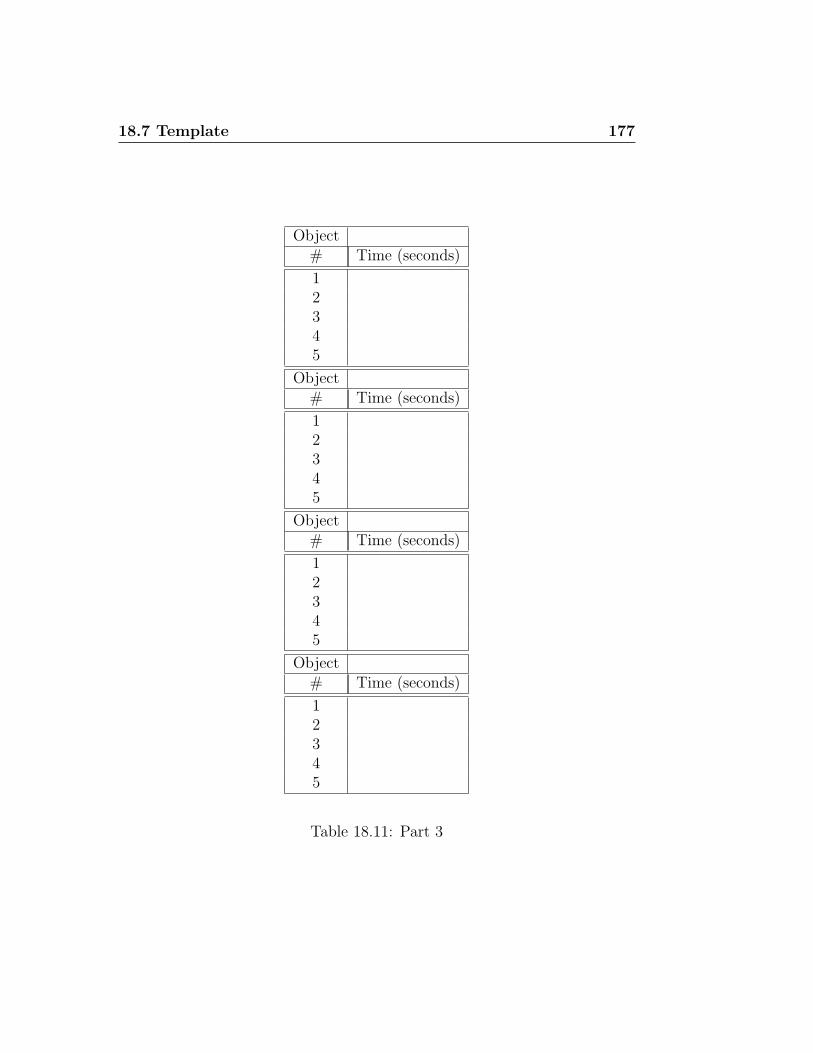
18.7 Template 177

Object# Time (seconds)

12345

Object# Time (seconds)

12345

Object# Time (seconds)

12345

Object# Time (seconds)

12345

Table 18.11: Part 3

178 Moment of Inertia

Chapter 19

Translational Equilibrium

19.1 Purpose

The object of this experiment is to study several systems in translationalequilibrium. By doing so, the first condition for equilibrium will be verified,the expression relating frictional force to normal force will be verified, andthe coefficient of kinetic friction for a pair of surfaces will be measured.

19.2 Introduction

This experiment will develop skills in vector analysis and determining uncer-tainties in trigonometric quantities. Remember to convert angles to radiansfor uncertainty calculations.

19.3 Theory

19.3.1 General

A body at rest or moving with constant velocity is in translational equi-librium, and thus consistent with Newton’s First Law the vector sum of allforces acting on it must be zero. In other words,

180 Translational Equilibrium

Σ~F = 0 (19.1)

ΣFX = 0 (19.2)

ΣFY = 0 (19.3)

ΣFZ = 0 (19.4)

If the lines of action of the forces acting on a body meet at one point,the forces are said to be concurrent. Concurrent forces cannot cause rota-tion and thus the above equations guarantee complete equilibrium for suchsituations.

19.3.2 Friction

There are two general classes of frictional forces which you will normallyconsider; static friction and kinetic (or sliding) friction.

Let us first consider the case of static friction. Suppose a block of weightw is resting on a plane surface as in Figure 19.1. Because there is no verticalmotion of the block, there must be a force equal and opposite to the force ofgravity, the normal force, N , also acting on the block. So, vertically thereare two forces acting on the body; a force down due to gravity, of magnitudew, and a force up due to the normal reaction, of magnitude N , and obviouslyw = N . Now, suppose that a force T is exerted on the block in a horizontaldirection, say from left to right. When T is very small the block will notmove. As T becomes larger there becomes a point at which the block willjust begin to move. The force which originally prevented the block frommoving is the force of static friction. At the value of T for which the blockjust starts to move, the force of static friction, fs, is just equal to T .

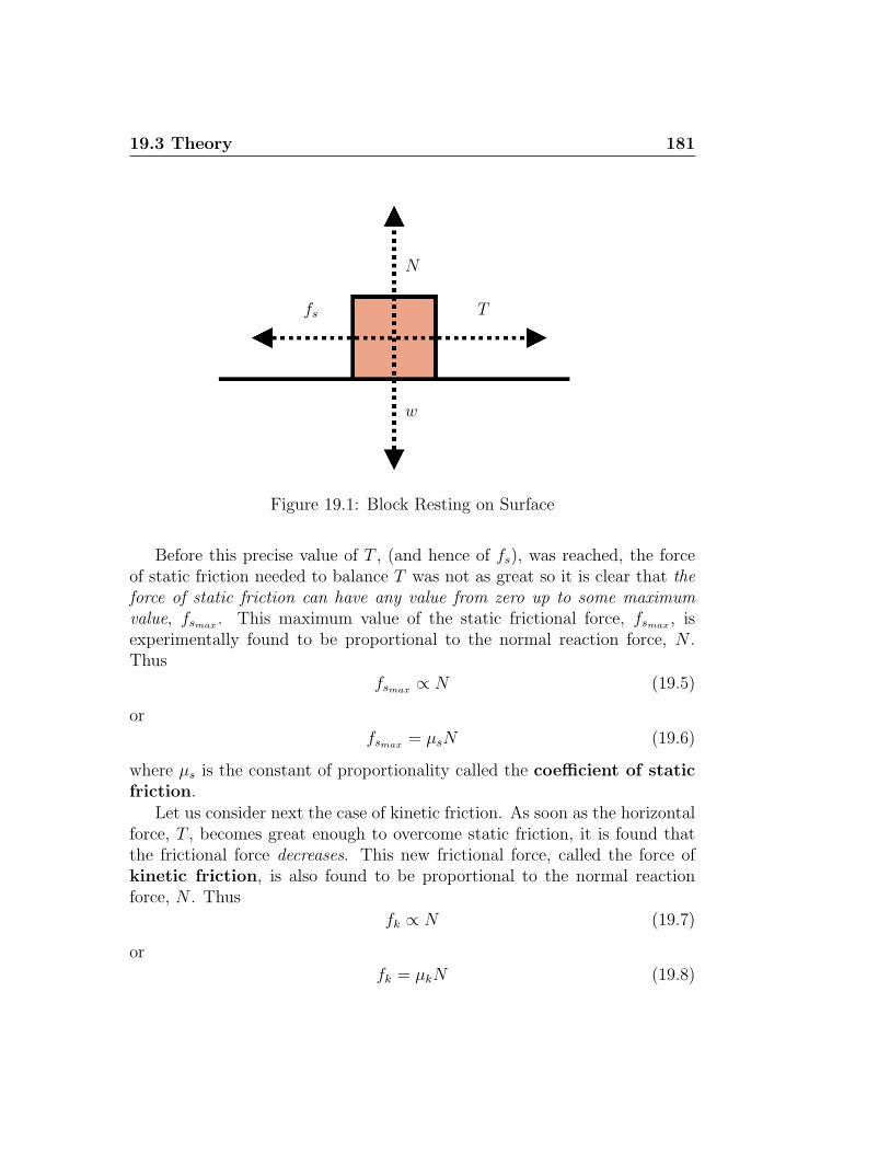
19.3 Theory 181

N

fs T

w

Figure 19.1: Block Resting on Surface

Before this precise value of T , (and hence of fs), was reached, the forceof static friction needed to balance T was not as great so it is clear that theforce of static friction can have any value from zero up to some maximumvalue, fsmax . This maximum value of the static frictional force, fsmax , isexperimentally found to be proportional to the normal reaction force, N .Thus

fsmax ∝ N (19.5)

or

fsmax = µsN (19.6)

where µs is the constant of proportionality called the coefficient of staticfriction.

Let us consider next the case of kinetic friction. As soon as the horizontalforce, T , becomes great enough to overcome static friction, it is found thatthe frictional force decreases. This new frictional force, called the force ofkinetic friction, is also found to be proportional to the normal reactionforce, N . Thus

fk ∝ N (19.7)

or

fk = µkN (19.8)

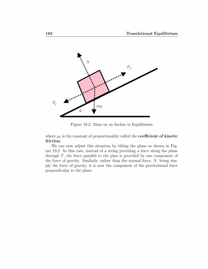
182 Translational Equilibrium

N

θmg

Ff

Fg

Figure 19.2: Mass on an Incline in Equilibrium

where µk is the constant of proportionality called the coefficient of kineticfriction.

We can now adjust this situation by tilting the plane as shown in Fig-ure 19.2. In this case, instead of a string providing a force along the planethrough T , the force parallel to the plan is provided by one component ofthe force of gravity. Similarly, rather than the normal force, N , being sim-ply the force of gravity, it is now the component of the gravitational forceperpendicular to the plane.

19.4 Procedure 183

The normal force is given by

N = mg cos θ

and the force pulling the block down the plane is

Fg = mg sin θ

From above, the frictional force is given by

Ff = µN

and so in equilibriumFg = Ff

ormg sin θ = µ (mg cos θ)

and thusµ = tan θ (19.9)

19.4 Procedure

19.4.1 Preparation

Pre-lab Questions

PQ1: What were the realistic uncertainties in the angles you determined inthe “Measuring Instruments” exercise? What were the factors responsiblefor them? Describe briefly how you determined them.

Pre-lab Tasks

PT1: From Equation 19.9, determine the equation for ∆µ, given ∆θ. Copythis into Table 19.4.

PT2: Copy the equation you determined for ∆Tx in the “Processing Uncer-tainties” exercise into Table 19.4.

PT3: Determine the equation for ∆Ty, which should be similar to what yougot in the previous task. Copy this into Table 19.4.

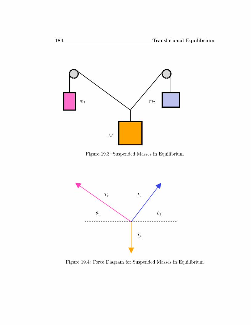
184 Translational Equilibrium

M

m1 m2

Figure 19.3: Suspended Masses in Equilibrium

T1

θ1

T2

θ2

T3

Figure 19.4: Force Diagram for Suspended Masses in Equilibrium

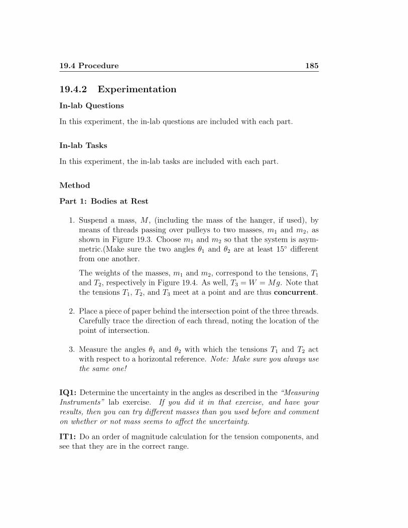
19.4 Procedure 185

19.4.2 Experimentation

In-lab Questions

In this experiment, the in-lab questions are included with each part.

In-lab Tasks

In this experiment, the in-lab tasks are included with each part.

Method

Part 1: Bodies at Rest

1. Suspend a mass, M , (including the mass of the hanger, if used), bymeans of threads passing over pulleys to two masses, m1 and m2, asshown in Figure 19.3. Choose m1 and m2 so that the system is asym-metric.(Make sure the two angles θ1 and θ2 are at least 15◦ differentfrom one another.

The weights of the masses, m1 and m2, correspond to the tensions, T1

and T2, respectively in Figure 19.4. As well, T3 = W = Mg. Note thatthe tensions T1, T2, and T3 meet at a point and are thus concurrent.

2. Place a piece of paper behind the intersection point of the three threads.Carefully trace the direction of each thread, noting the location of thepoint of intersection.

3. Measure the angles θ1 and θ2 with which the tensions T1 and T2 actwith respect to a horizontal reference. Note: Make sure you always usethe same one!

IQ1: Determine the uncertainty in the angles as described in the “MeasuringInstruments” lab exercise. If you did it in that exercise, and have yourresults, then you can try different masses than you used before and commenton whether or not mass seems to affect the uncertainty.

IT1: Do an order of magnitude calculation for the tension components, andsee that they are in the correct range.

186 Translational Equilibrium

Part 2: Body Traveling at Constant Velocity

1. Place the block on the plane with the plane horizontal and increase theangle of elevation of the plane until the block slides at constant velocityafter you tap it to get it moving. Repeat this a few times being carefulnot to jiggle the plane. Record the elevation angles in Table 19.7.

Your uncertainty in the angle may be due to having to judge when the blockis moving at “constant” velocity. This is a valid uncertainty, since anyonewill have the same problem. Be sure to discuss how you did this.

IQ2: Determine the uncertainty in the angles as described in the “MeasuringInstruments” lab exercise. Describe briefly what you did.

IT2: Do an order of magnitude calculation for µ.

Part 3: Body At Rest, on the Verge of Motion

1. Now place the block on the plane and increase the angle of elevation ofthe plane until the block begins to slide on its own. Repeat this a fewtimes being careful not to jiggle the plane. Record the elevation anglesin Table 19.8.

In this case, you don’t have to judge anything, since the block is either movingor not. The uncertainty will come from the consistency of determining theangle at which the block starts to move.

IQ3: Determine the uncertainty in the angles as described in the “MeasuringInstruments” lab exercise. Describe briefly what you did.

IQ4: Were the angles for one coefficient of friction more consistent than forthe other? Discuss.

IT3: Do an order of magnitude calculation for µ, and see that it makes sensegiven the previous value.

19.4.3 Analysis

Post-lab Discussion Questions

In this experiment, the post-lab questions are included with each part.

19.4 Procedure 187

Post-lab Tasks

In this experiment, the post-lab tasks are included with each part.

Part 1: Bodies at Rest

1. Record the magnitudes of T1, T2, and T3 as well as their respectiveangles in a table.

2. Resolve the three tensions into their x and y components.

3. Add up the horizontal and vertical components separately to determinewhether the expected equilibrium conditions were achieved.

T1: Do a proper statistical analysis, (ie. calculate standard deviation, etc.)for each of the angles to determine the uncertainty in the angles. How doesit compare to what you determined back in the “Measuring Instruments”exercise? (In other words, did you need to do the statistical calculations orwas your original determination fairly accurate1?)

Q1: Were the conditions for static equilibrium achieved within experimentaluncertainty?

Part 2: Body Traveling at Constant Velocity

Calculate the average angle. Use this to determine the coefficient of kineticfriction, µk, according to the equation

µk = tan(θ)

(19.10)

where θ = elevation angle of the plane. Repeat the experiment and recordthe results.

T2: Do a proper statistical analysis, (ie. calculate standard deviation, etc.)for the angle to determine the uncertainty.

Part 3: Body At Rest, on the Verge of Motion

1Remember that uncertainties are only quoted to one or two significant figures; if twodifferent methods of calculating uncertainty are the same to one significant figure, thenthey are equally good.

188 Translational Equilibrium

Calculate the average angle. Use this to determine the coefficient of staticfriction, µs, according to the equation

µs = tan(θ)

(19.11)

where θ is the angle of elevation of the plane.

T3: Do a proper statistical analysis, (ie. calculate standard deviation, etc.)for the angle to determine the uncertainty.

Q2: Compare the values calculated for µs and µk. Do they agree withinexperimental uncertainty?

19.5 Bonus

From Part 1, use the polygon (graphical) method of vector addition to graph-ically check for equilibrium using the measured forces T1, T2, and T3. Canyou include uncertainties when using the graphical method? If so, explain(show?) how. If not, explain why not.

19.6 Weightings

Pre-lab Questions and Tasks 5In-lab Questions and Tasks 10Post-lab Questions and Tasks 10Template 5Report 70Bonus 5

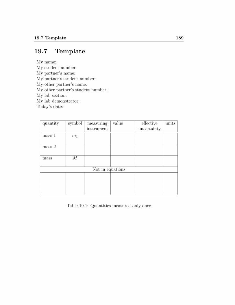
19.7 Template 189

19.7 Template

My name:My student number:My partner’s name:My partner’s student number:My other partner’s name:My other partner’s student number:My lab section:My lab demonstrator:Today’s date:

quantity symbol measuring value effective unitsinstrument uncertainty

mass 1 m1

mass 2

mass M

Not in equations

Table 19.1: Quantities measured only once

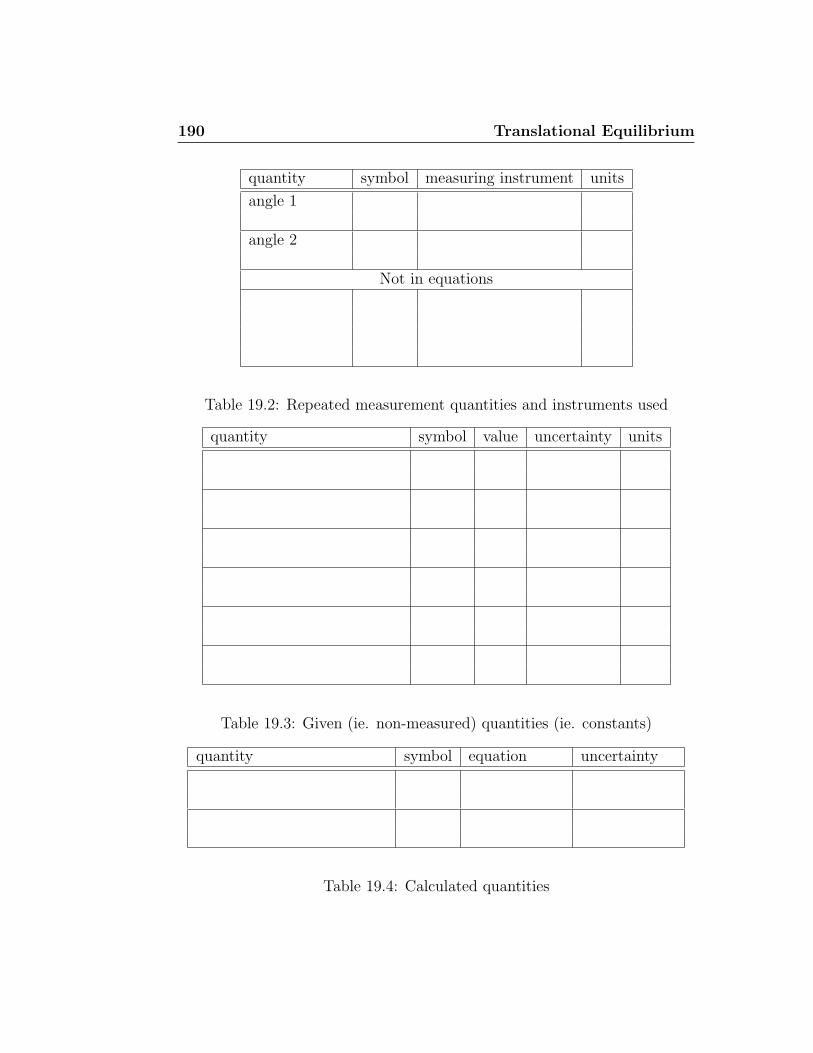
190 Translational Equilibrium

quantity symbol measuring instrument units

angle 1

angle 2

Not in equations

Table 19.2: Repeated measurement quantities and instruments used

quantity symbol value uncertainty units

Table 19.3: Given (ie. non-measured) quantities (ie. constants)

quantity symbol equation uncertainty

Table 19.4: Calculated quantities

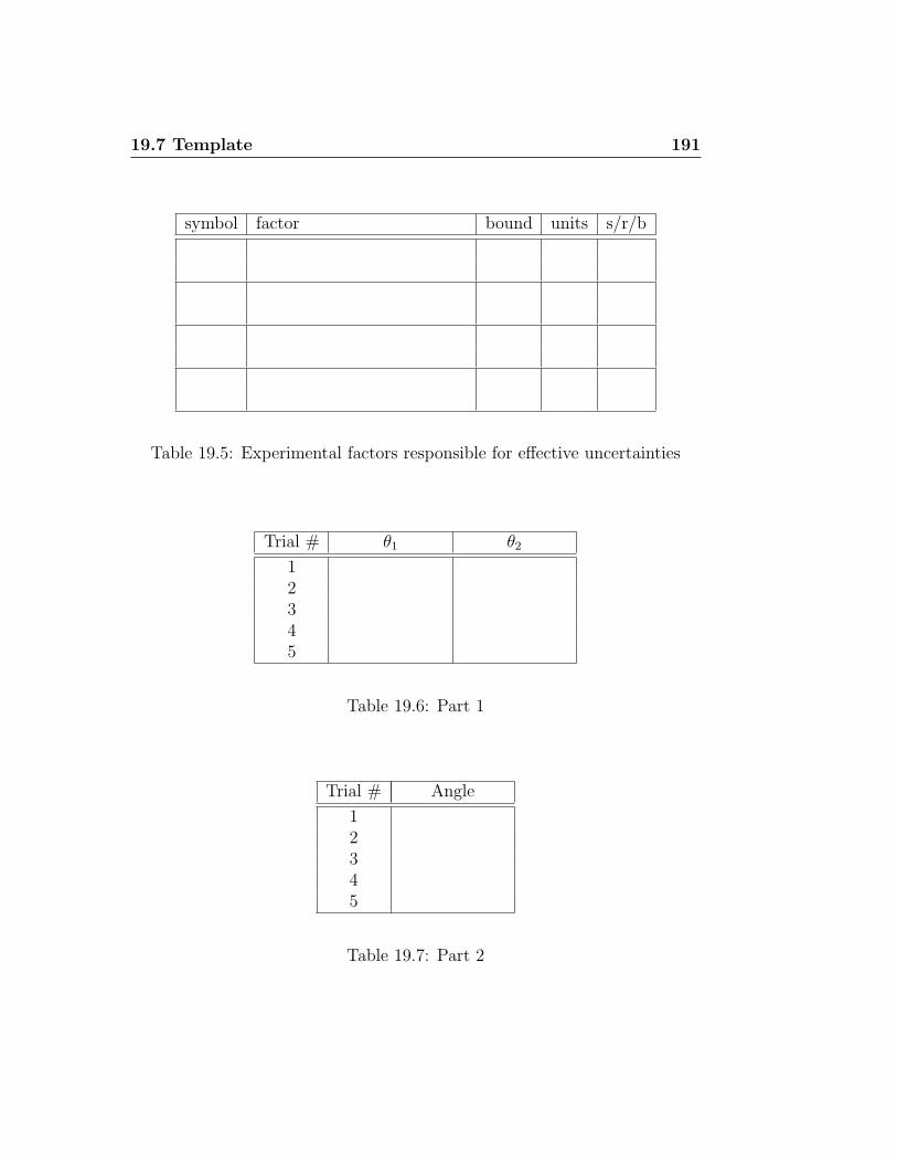
19.7 Template 191

symbol factor bound units s/r/b

Table 19.5: Experimental factors responsible for effective uncertainties

Trial # θ1 θ2

12345

Table 19.6: Part 1

Trial # Angle

12345

Table 19.7: Part 2

192 Translational Equilibrium

Trial # Angle

12345

Table 19.8: Part 3

Chapter 20

One Dimensional Conservationof Momentum and Energy

20.1 Purpose

The purpose of this experiment is to study the conservation of momentumand energy in one dimension by examining the motion of colliding carts ona track.

20.2 Introduction

The method employed in this experiment is much like any which use the cartsand track. This experiment will require calculations with repeated dependentmeasurements.

20.3 Theory

For bodies traveling in one dimension, position and velocity can be simplyspecified; position will be a distance from the origin, and velocity will beeither positive or negative based on the direction of travel. (For instance, anobject traveling to the right may be considered to have a positive velocity,while one traveling to the left will have a negative velocity. When two objectsmoving in one dimension collide, the following conditions hold:

Initial momentum = Pi = m1v1i + m2v2i (20.1)

194 One Dimensional Conservation of Momentum and Energy

Initial energy = Ei =1

2m1v

21i +

1

2m2v

22i (20.2)

Final momentum = Pf = m1v1f + m2v2f (20.3)

Final energy = Ef =1

2m1v

21f +

1

2m2v

22f (20.4)

Since velocities can be positive or negative, this means that in the aboveequations, momentum can be positive or negative, while energy must alwaysbe positive (unless it is zero, in which case there is no motion.)

For any collision, momentum should be conserved. However, energy willonly be conserved if a collision is elastic.

20.4 Procedure

20.4.1 Preparation

Pre-lab Tasks

PT1: Copy the equations you determined for ∆P and ∆E in the “ProcessingUncertainties” exercise into Table 20.4.

Pre-lab Questions

PQ1: Given x̄ and t̄, as well as ∆x̄ and ∆t̄ for a cart, determine the equationfor ∆v.

PQ2: How could you tell if the track was not level by the motion of thecarts before and after the collision? Could you tell which way the track wassloped?

PQ3: How would the effects of friction show up in the data from the carts?

20.4.2 Experimentation

Make sure the track is level before you begin this experiment.Do not use equal masses for your experiment.Make sure that the carts do not actually make contact with each other or elsethe collision will be definitely inelastic.

20.4 Procedure 195

1. Without recording data, try a sample collision by having one cart col-lide with the other which is initially at rest. Then do the same thingthe other way around, i.e. the cart which was previously at rest willnow be the one initially moving.

2. Now change the mass difference between the carts and repeat. Fromthe four options you have tried, choose the method which you believeshould give you the best results.

3. Measure the masses of the carts with their uncertainties.

4. Measure the “ladder” spacing with its possible error.

In this case, when the spacing of the individual bars should be veryconsistent, the best way to determine the spacing is to measure thedistance for all thirteen bars, and divide in order to get the length ofany sub-interval. Be sure to count and measure intervals, not bars.

5. Perform the experiment as stated above.

In-lab Tasks

IT1: Do an order of magnitude calculation for each of P and E, using singletime intervals, before and after.

In-lab Questions

IQ1: Sketch the ladder, and show what distance you measured on the sketchand what value you got, with its uncertainty.

IQ2: Sketch the output from the software as four blocks of data, and indicatewhat each block represents; eg. cart 1 before, etc.

IQ3: If you are using a disk to save your data, fill in the first value in eachcolumn of the template to ensure you know which dataset is which.

IQ4: Explain your choice of which collision to use; ie. state what factor(s)caused you to reject the other options.

196 One Dimensional Conservation of Momentum and Energy

20.4.3 Analysis

1. Calculate the velocities of both carts before and after the collision usingthe method of differences, and state the results with their possibleerrors.

2. Calculate both momentum and energy of the two carts before and afterthe collision, as well as the total energy before and after the collision.State them with their associated errors and determine whether or notmomentum and energy were conserved.

Post-lab Discussion Questions

Q1: Did your data indicate whether or not the track was indeed level? How?

Q2: Was momentum conserved within your experimental uncertainties?

Q3: Was energy conserved within your experimental uncertainties?

20.5 Bonus: Inelastic Collisions

Learn how to perform an inelastic collision and do so. Was energy conserved?Was momentum conserved? (You will find having your spreadsheet alreadycreated makes this easy.)

20.6 Weightings

Pre-lab Questions 5In-lab Questions 10Post-lab Questions 10Template 5Report 70

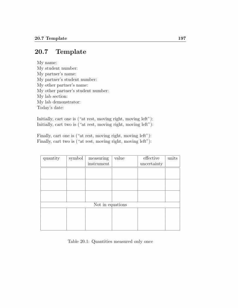
20.7 Template 197

20.7 Template

My name:My student number:My partner’s name:My partner’s student number:My other partner’s name:My other partner’s student number:My lab section:My lab demonstrator:Today’s date:

Initially, cart one is (“at rest, moving right, moving left”):Initially, cart two is (“at rest, moving right, moving left”):

Finally, cart one is (“at rest, moving right, moving left”):Finally, cart two is (“at rest, moving right, moving left”):

quantity symbol measuring value effective unitsinstrument uncertainty

Not in equations

Table 20.1: Quantities measured only once

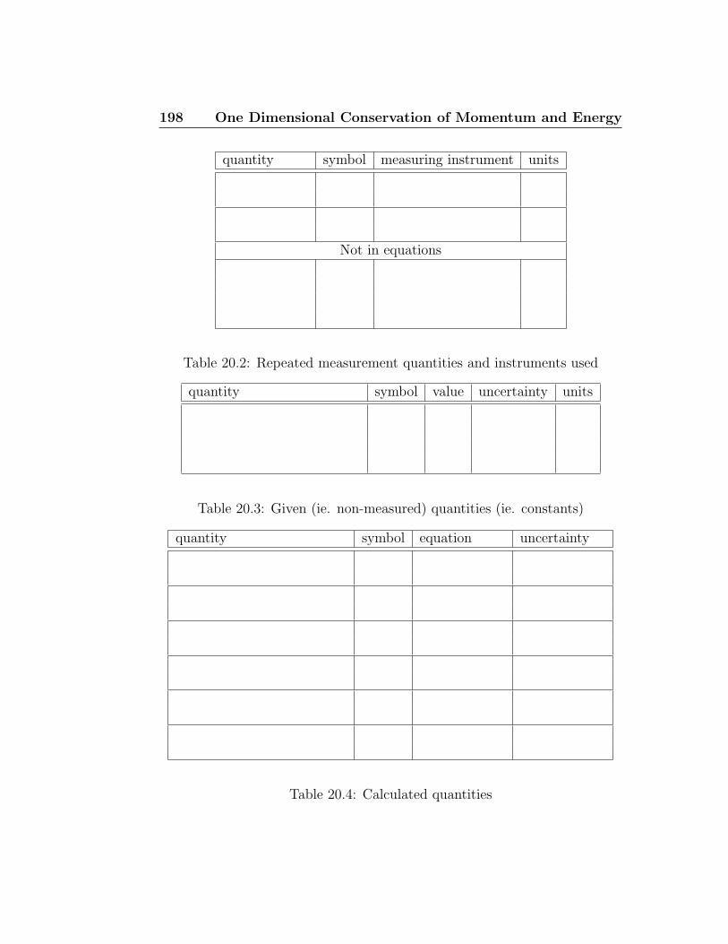
198 One Dimensional Conservation of Momentum and Energy

quantity symbol measuring instrument units

Not in equations

Table 20.2: Repeated measurement quantities and instruments used

quantity symbol value uncertainty units

Table 20.3: Given (ie. non-measured) quantities (ie. constants)

quantity symbol equation uncertainty

Table 20.4: Calculated quantities

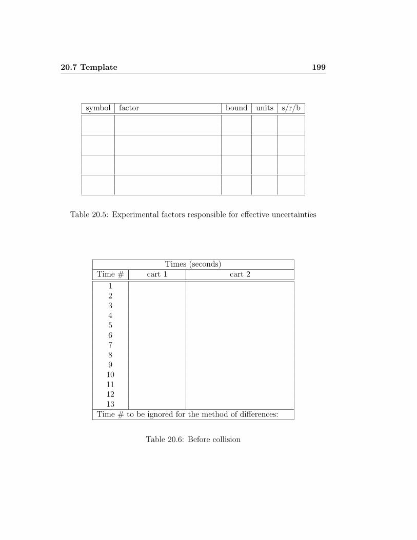
20.7 Template 199

symbol factor bound units s/r/b

Table 20.5: Experimental factors responsible for effective uncertainties

Times (seconds)Time # cart 1 cart 2

12345678910111213

Time # to be ignored for the method of differences:

Table 20.6: Before collision

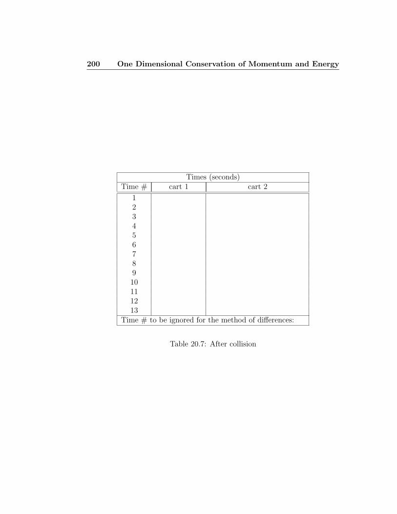
200 One Dimensional Conservation of Momentum and Energy

Times (seconds)Time # cart 1 cart 2

12345678910111213

Time # to be ignored for the method of differences:

Table 20.7: After collision

Chapter 21

Torque and the Principle ofMoments

21.1 Purpose

The object of this experiment is to study and understand the concepts oftorque and static equilibrium of a body.

21.2 Introduction

This experiment should help the student become familiar with simple calcu-lations with uncertainties.

21.3 Theory

In order for a rigid body to remain in equilibrium, the following two condi-tions must be satisfied:

1. the resultant external force acting on the body must be zero.

2. the sum of the moments (torques) acting in a counter-clockwise direc-tion about any point must equal the sum of the clockwise momentsabout the same point. (This is the Principle of Moments.

The body is in static equilibrium if it is at rest with respect to its frame ofreference (which in this case would be the lab table).

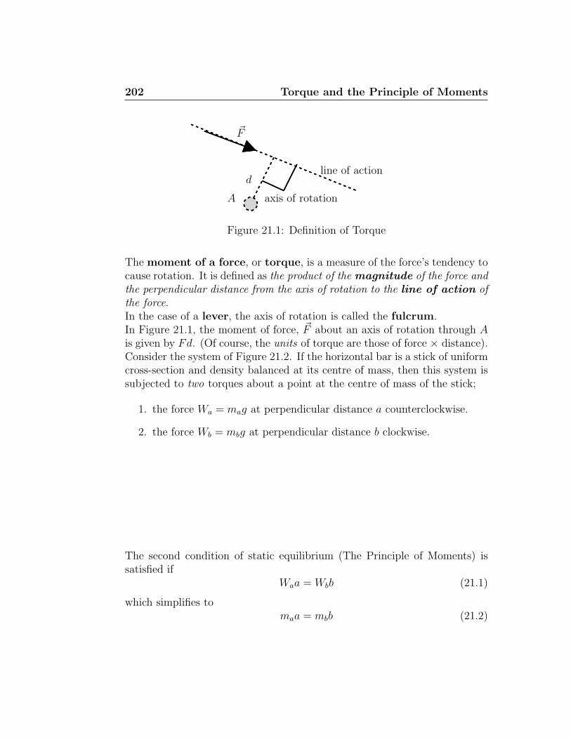
202 Torque and the Principle of Moments

A axis of rotation

d

~F

line of action

Figure 21.1: Definition of Torque

The moment of a force, or torque, is a measure of the force’s tendency tocause rotation. It is defined as the product of the magnitude of the force andthe perpendicular distance from the axis of rotation to the line of action ofthe force.In the case of a lever, the axis of rotation is called the fulcrum.In Figure 21.1, the moment of force, ~F about an axis of rotation through Ais given by Fd. (Of course, the units of torque are those of force × distance).Consider the system of Figure 21.2. If the horizontal bar is a stick of uniformcross-section and density balanced at its centre of mass, then this system issubjected to two torques about a point at the centre of mass of the stick;

1. the force Wa = mag at perpendicular distance a counterclockwise.

2. the force Wb = mbg at perpendicular distance b clockwise.

The second condition of static equilibrium (The Principle of Moments) issatisfied if

Waa = Wbb (21.1)

which simplifies tomaa = mbb (21.2)

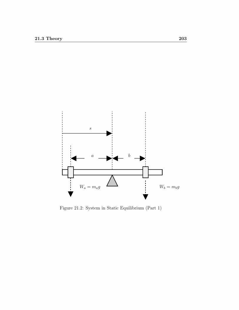
21.3 Theory 203

Wa = mag Wb = mbg

a b

s

Figure 21.2: System in Static Equilibrium (Part 1)

204 Torque and the Principle of Moments

21.4 Procedure

21.4.1 Preparation

Pre-lab Questions

PQ1: For the system in Figure 21.2, determine the equations for ∆τcw and∆τccw, given a, b, ma, mb, ∆a, ∆b, ∆ma and ∆mb.

Pre-lab Tasks

PT1: Copy the above equations into Table 21.4

21.4.2 Experimentation

Apparatus

Uniform and non-uniform meter sticks, 3 meter stick clamps with knife-edgeload supports, a 2 kg range spring scale, a set of hooked weights, a laboratorybalance and a support stand.

In-lab Questions

In this experiment, the in-lab questions are included with each part.

Part 1: Testing the Principle of Moments

1. Place one metre stick clamp near the centre of the uniform metre stickand suspend this combination from the suspension point mentionedabove so that the zero cm mark of the metre stick is at the left end.

2. Find the centre of mass of the metre stick by sliding it in its clamp1

until it lies horizontally at rest. Record this position, s.

3. Adjust the clamp slightly to determine how far you can move it until thestick is noticeably not horizontal. Use this to determine the uncertainty∆s.

1In this experiment, the terms “hanger” and “clamp” will both be used to describe thesame piece of equipment. This is because the function is slightly different in each case.

21.4 Procedure 205

4. Weigh the two remaining clamps and record their masses.

5. With the metre stick as above, suspend a weight from a hanger on eachside of the centre of mass, as in Figure 21.2. Use mb ≥ 2ma so that youget very different distances for a and b. When adjusting the position ofthe second mass for equilibrium, use the same procedure used earlierfor ∆s to determine the uncertainty in the position of the second mass.

IQ1: Why do you not need to experimentally find the uncertainty in thepositions of both masses?

Note that ma and mb include the masses of their respective hangers.

Part 2: Mass and Center of Mass Determination from a SingleEquilibrium Setup

1. Check to see if the spring scale reads zero when unloaded. If it doesn’t,be sure to record the zero error with its uncertainty for use later in thisexperiment. Hang the spring scale from the system support.

2. Suspend a 200g mass from a hanger between the 10 and 20 cm marksof the metre stick as in Figure 21.3 and record the metre stick readingat the position of the hanger (c in the diagram).

3. Support the system by a hanger which is attached to the spring scaleand to the metre stick between the suspension point of the 200g massand the known centre of mass of the stick. Record the metre stickreading, s, at the point of suspension. In this case, only m, the metrestick mass, is unknown. It can be determined by either of the conditionsrequired for static equilibrium:∑

Fext = 0 (21.3)

and ∑τext = 0 (21.4)

Equating forces up to forces down

W = Fa + f + f ′ (21.5)

orM = ma + m + m′ (21.6)

where

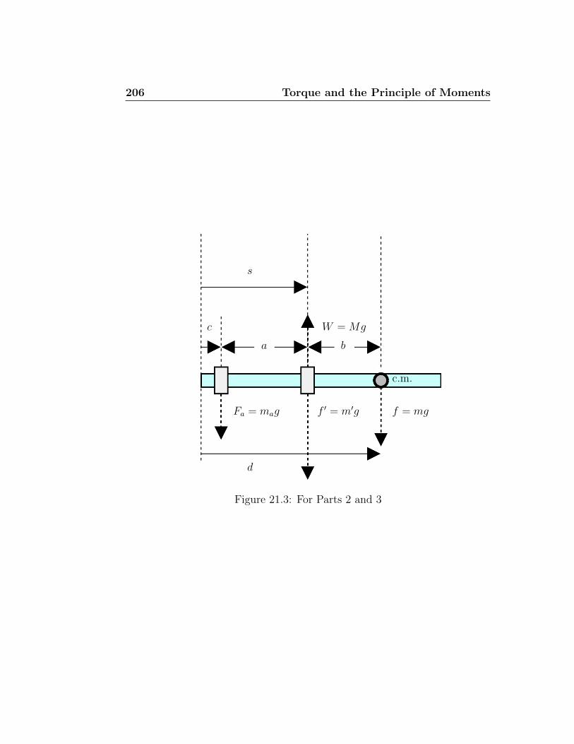
206 Torque and the Principle of Moments

Fa = mag f ′ = m′g f = mg

W = Mg

c.m.

s

a b

c

d

Figure 21.3: For Parts 2 and 3

21.4 Procedure 207

• M is the total suspended mass, read from the spring scale

• m is the mass of the metre stick

• m′ is the mass of the clamp at the point of suspension

• ma is the suspended mass (including the clamp at a)

Thus, m is obtained from

m = M −ma −m′ (21.7)

From Equation 21.4, the sum of the counterclockwise torques aboutany point equal the sum of the clockwise torques about that point.Thus, about the point of suspension

Faa = fb (21.8)

ormaa = mb (21.9)

and finallym = (a/b)ma (21.10)

4. Find d directly as in Part 1.

5. Measure the mass of the metre stick using the balance in the lab.

Part 3: The Non–Uniform Metre Stick

1. Set up the non-uniform metre stick set up exactly as in Part 2. Againwe have two unknowns:

(a) m, the metre stick mass, and

(b) d, the distance from the zero end of the stick to the centre of mass.

2. Repeat the measurements as in Part 2.

3. Find d directly as in Part 1.

4. Measure m on the lab scale.

IQ2: Does the position of the centre of mass of the non-uniform metre stickmake sense given where the holes are?

IQ3: Given what you know about torques, which holes make the biggestcontribution to moving the centre of mass away from the 50cm mark?

208 Torque and the Principle of Moments

21.4.3 Analysis

Part 1: Testing the Principle of Moments

1. Calculate to clockwise and counterclockwise torques to see if the Prin-ciple of Moments was obeyed.

Part 2: Mass and Center of Mass Determination from a SingleEquilibrium Setup

1. Using Equation 21.7, calculate the mass of the metre stick.

2. Using Equation 21.10, and the mass calculated above, calculate thedistance b to the centre of mass of the metre stick.

3. Use the metre stick reading for the point of suspension s recordedearlier and b to calculate d, the reading on the metre stick at the centreof mass.

4. Compare your calculated and measured values for d and m.

Part 3: The Non–Uniform Metre Stick

1. Perform a similar analysis to that for Part 2 above.

Post-lab Discussion Questions

Q1: Was the Principle of Moments obeyed for the system in Part 1? Explain.

Q2: Did the measured and calculated masses for the metre stick in Part 2agree?

Q3: Did the the measured position of the centre of mass in Part 2 agree withthe value calculated?

Q4: Did the measured and calculated metre stick masses in Part 3 agree?

Q5: Did the the measured position of the centre of mass in Part 3 agree withthe value calculated?

21.5 Bonus: Unknown Metre Stick and Unknown Mass 209

21.5 Bonus: Unknown Metre Stick and Un-

known Mass

Given

1. a non–uniform metre stick of unknown mass and centre of mass

2. an object of unknown mass,

3. one object of known mass,

4. assorted hangers of known mass,

and NO spring scale, explain how you could determine the mass of the object.Time permitting, try it and discuss your results.

21.6 Weightings

Pre-lab Questions 5In-lab Questions 10Post-lab Questions 10Template 5Report 70Bonus 5

210 Torque and the Principle of Moments

21.7 Template

My name:My student number:My partner’s name:My partner’s student number:My other partner’s name:My other partner’s student number:My lab section:My lab demonstrator:Today’s date:

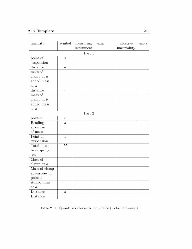
21.7 Template 211

quantity symbol measuring value effective unitsinstrument uncertainty

Part 1point of ssuspensiondistance amass ofclamp at aadded massat adistance bmass ofclamp at badded massat b

Part 2position cReading dat centreof massPoint of ssuspensionTotal mass Mfrom springscaleMass ofclamp at aMass of clampat suspensionpoint sAdded massat aDistance aDistance b

Table 21.1: Quantities measured only once (to be continued)

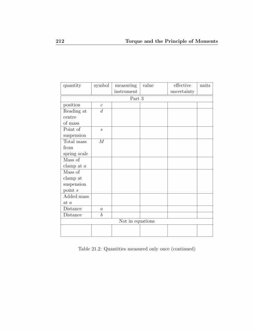
212 Torque and the Principle of Moments

quantity symbol measuring value effective unitsinstrument uncertainty

Part 3position cReading at dcentreof massPoint of ssuspensionTotal mass Mfromspring scaleMass ofclamp at aMass ofclamp atsuspensionpoint sAdded massat aDistance aDistance b

Not in equations

Table 21.2: Quantities measured only once (continued)

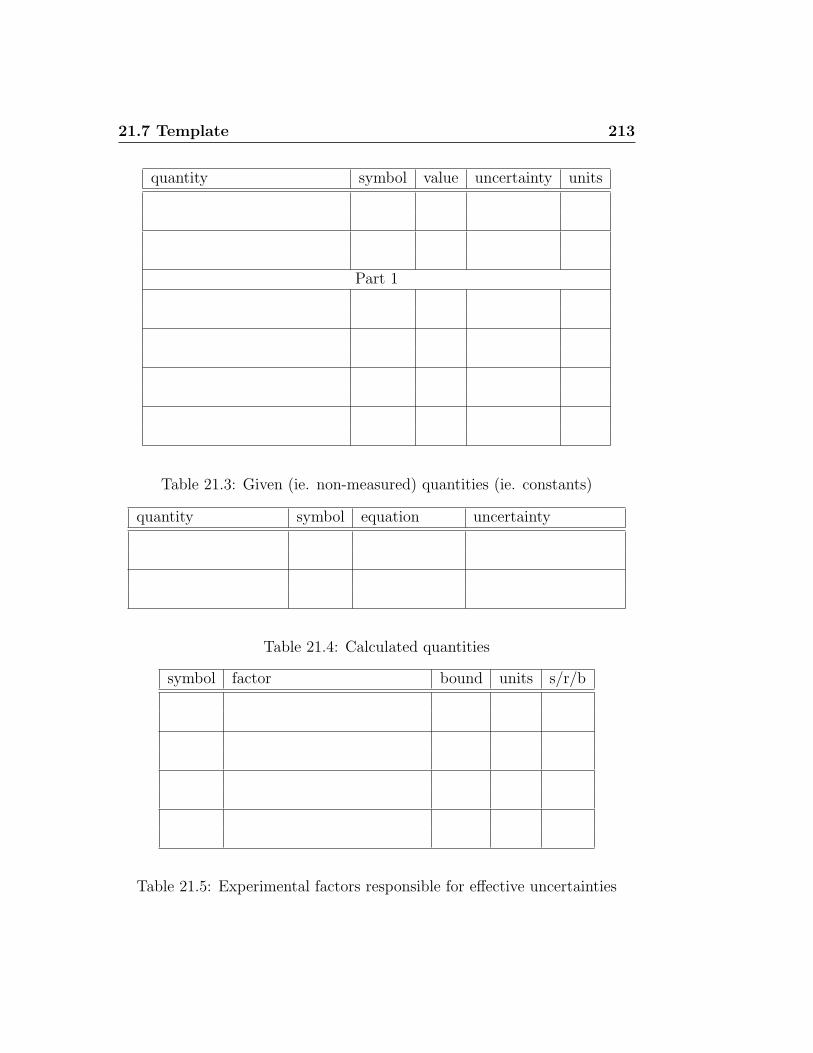
21.7 Template 213

quantity symbol value uncertainty units

Part 1

Table 21.3: Given (ie. non-measured) quantities (ie. constants)

quantity symbol equation uncertainty

Table 21.4: Calculated quantities

symbol factor bound units s/r/b

Table 21.5: Experimental factors responsible for effective uncertainties

214 Torque and the Principle of Moments

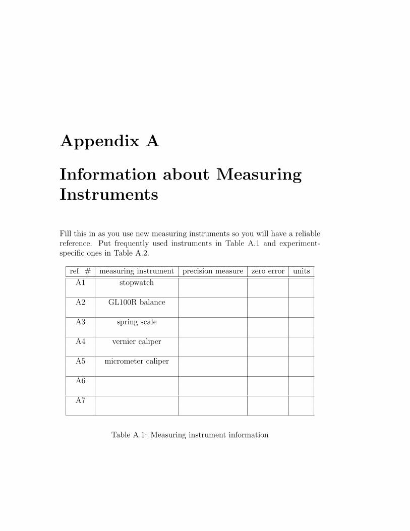
Appendix A

Information about MeasuringInstruments

Fill this in as you use new measuring instruments so you will have a reliablereference. Put frequently used instruments in Table A.1 and experiment-specific ones in Table A.2.

ref. # measuring instrument precision measure zero error units

A1 stopwatch

A2 GL100R balance

A3 spring scale

A4 vernier caliper

A5 micrometer caliper

A6

A7

Table A.1: Measuring instrument information

216 Information about Measuring Instruments

ref. # measuring instrument precision measure zero error units

B1

B2

B3

B4

B5

B6

B7

B8

B9

B10

B11

B12

B13

B14

B15

Table A.2: Measuring instrument information (continued)

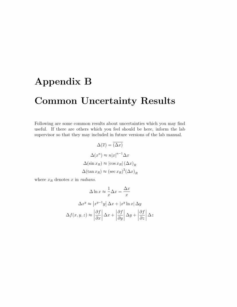
Appendix B

Common Uncertainty Results

Following are some common results about uncertainties which you may finduseful. If there are others which you feel should be here, inform the labsupervisor so that they may included in future versions of the lab manual.

∆(x) = (∆x)

∆(xn) ≈ n|x|n−1∆x

∆(sin xR) ≈ |cos xR| (∆x)R

∆(tan xR) ≈ (sec xR)2(∆x)R

where xR denotes x in radians.

∆ ln x ≈ 1

x∆x =

∆x

x

∆xy ≈∣∣xy−1y

∣∣∆x + |xy ln x|∆y

∆f(x, y, z) ≈∣∣∣∣∂f

∂x

∣∣∣∣∆x +

∣∣∣∣∂f

∂y

∣∣∣∣∆y +

∣∣∣∣∂f

∂z

∣∣∣∣∆z

218 Common Uncertainty Results

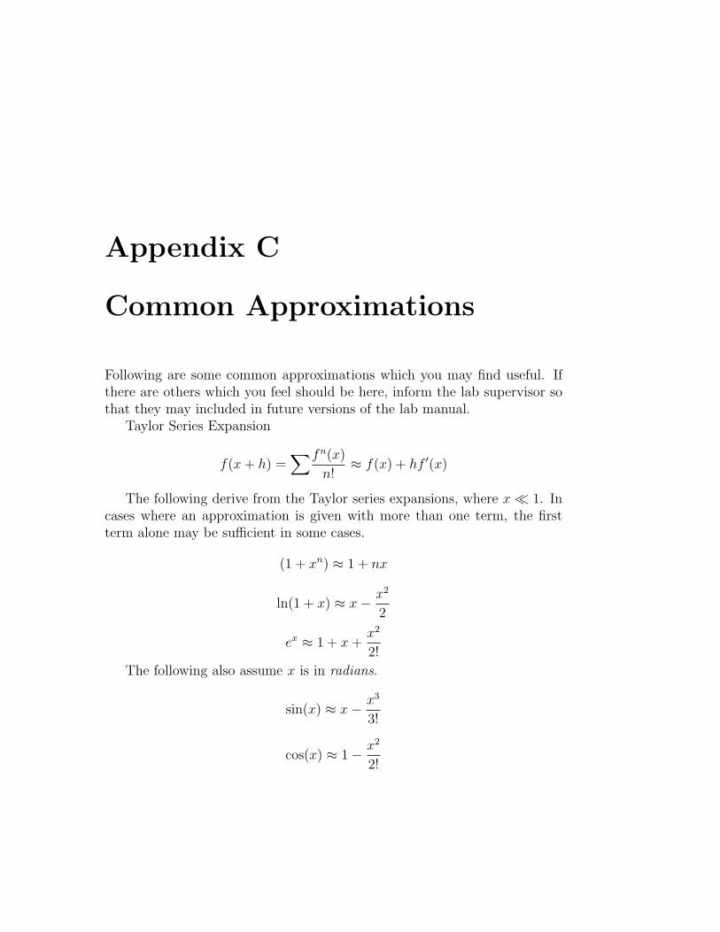
Appendix C

Common Approximations

Following are some common approximations which you may find useful. Ifthere are others which you feel should be here, inform the lab supervisor sothat they may included in future versions of the lab manual.

Taylor Series Expansion

f(x + h) =∑fn(x)

n!≈ f(x) + hf ′(x)

The following derive from the Taylor series expansions, where x � 1. Incases where an approximation is given with more than one term, the firstterm alone may be sufficient in some cases.

(1 + xn) ≈ 1 + nx

ln(1 + x) ≈ x− x2

2

ex ≈ 1 + x +x2

2!

The following also assume x is in radians.

sin(x) ≈ x− x3

3!

cos(x) ≈ 1− x2

2!

220 Common Approximations

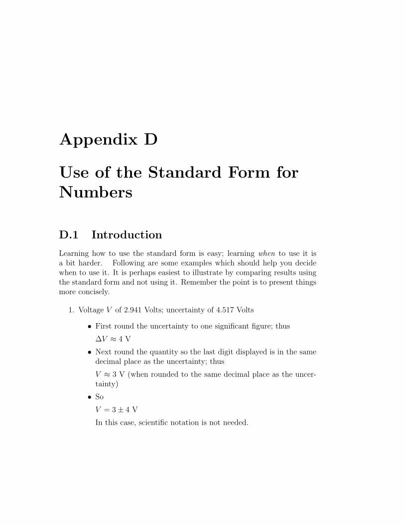
Appendix D

Use of the Standard Form forNumbers

D.1 Introduction

Learning how to use the standard form is easy; learning when to use it isa bit harder. Following are some examples which should help you decidewhen to use it. It is perhaps easiest to illustrate by comparing results usingthe standard form and not using it. Remember the point is to present thingsmore concisely.

1. Voltage V of 2.941 Volts; uncertainty of 4.517 Volts

• First round the uncertainty to one significant figure; thus

∆V ≈ 4 V

• Next round the quantity so the last digit displayed is in the samedecimal place as the uncertainty; thus

V ≈ 3 V (when rounded to the same decimal place as the uncer-tainty)

• So

V = 3± 4 V

In this case, scientific notation is not needed.

222 Use of the Standard Form for Numbers

2. Mass m of 140.6 grams; uncertainty of 531.7 grams

• First round the uncertainty to one significant figure; thus

∆m ≈ 500 g

• Next round the quantity so the last digit displayed is in the samedecimal place as the uncertainty; thus

m ≈ 100 g (when rounded to the hundreds place)

• So

m = 100± 500 g

In this case, scientific notation is needed, because we need to getrid of the placeholder zeroes. One option would be to write

m = (1± 5)× 102 g

Another option would be to write

m = 0.1± 0.5 kg

Note that this last option is more concise.

3. Diameter d of 0.727 cm; uncertainty of 0.015 cm

• First round the uncertainty to one significant figure; thus

∆d ≈ 0.02 cm

• Next round the quantity so the last digit displayed is in the samedecimal place as the uncertainty; thus

d ≈ 0.73 cm (when rounded to the hundredths place)

• So

d = 0.73± 0.02 cm

In this case, scientific notation is not needed, because there areno placeholder zeroes.

Another option would be to write

d = 7.3± 0.2 mm

Note that this last option is slightly more concise, since it getsrid of two zeroes, and puts d in proper form for scientific notation(even though in this case the exponent would be zero).

D.1 Introduction 223

4. Time t of 943 s; uncertainty of 29 s

• First round the uncertainty to one significant figure; thus

∆t ≈ 30 s

• Next round the quantity so the last digit displayed is in the samedecimal place as the uncertainty; thus

t ≈ 940 s (when rounded to the tens place)

• So

t = 940± 30 s

In this case, scientific notation is needed, because there are place-holder zeroes.

One option would be to write

t = (9.4± 0.3)× 102 s

This is in the standard form.

Another option would be to write

t = 9.4± 0.3 hs

However, since “hectoseconds” are not commonly used I wouldavoid this (although it is also correct).

Similarly you could write

t = 94± 3 das

Again, since “dekaseconds” are not commonly used I would avoidthis (although it is also correct).1

1I actually had to check on the spelling and notation for dekaseconds and hectoseconds,so that illustrates how (un)familiar they are.

224 Use of the Standard Form for Numbers

Appendix E

Order of MagnitudeCalculations

To check your conversions, (among other things), do a rough calculation ofyour results carrying every value to just 1 significant1 figure. (This is easy todo quickly on a piece of paper without a calculator, so you can be sure thatcalculated results are in the right ballpark.)For instance, for the “Measuring ‘g’ ” experiment,

h ≈ 5m

t ≈ 1s

Thus

g ≈ 2× 5

12≈ 10m/s2

Be sure to write out these calculations; that way you’ll be clear on the unitsyou used, etc. If you make an error and have to correct it, you’ll want arecord of it so you don’t make it when you do the “real” calculations.Since this result is about what you’d expect, then you know any values inthat range should be reasonable.

E.1 Why use just one or two digits?

There are a couple of reasons:

1If the digit is a 1 or a two, then you may carry 2 figures. If you do this then youranswer should be within about 10% of the value you’d get with a detailed calculation.This is easily close enough to spot any major errors.

226 Order of Magnitude Calculations

1. Since we’re only using one data point, instead of all of our values, theresult will be approximate, so the extra digits aren’t needed.

2. When people use calculators, they tend to just automatically writedown any answer without thinking. If they made a typing mistake,they often don’t notice. So by doing it by hand using only one or twodigits, they keep their brains engaged and are more likely to notice anerror.

E.2 Order of Magnitude Calculations for Un-

certainties

In a similar way, you can check to see if your uncertainties are reasonable.In the above example, if

∆h ≈ 5 cm

and∆t ≈ 0.1 s

then

∆g ≈ g

(∆h

h+ 2

∆t

t

)≈ 10

(0.05

5+ 2

0.1

1

)≈ 10 (0.01 + 0.2)

≈ 10 (0.21)

≈ 0.2 m/s2

This makes sense, and so your detailed uncertainty calculations should pro-duce something in this ballpark.

Index

calculations with uncertainties, 59,115

conservation of energy, 193conservation of momentum, 193

differencesmethod of, 53

digital scales, 85Discussion of Errors, 59, 115Discussion of Uncertainties, 59, 115

effective uncertainty, 83energy

conservation ofin one dimension, 193

equilibriumstatic, 201translational, 179

errorexperimental, 33zero, 38, 82

errorsdiscussion of, 59, 115random, 35systematic, 34

g, 145gravity

acceleration due to, 145

human reaction time, 93

inertiamoment of , 157

lab manual layout, 1lab manual templates, 5linear scales, 83

manuallayout of, 1

measurementuncertainty in, 35

measurementsrepeated, 103

dependent, 53method of differences, 53moment of inertia, 157moments

principle of, 201momentum

conservation ofin one dimension, 193

motionrotational, 157

operations with uncertainties, 59

precision measure, 35, 81digital instruments, 82non-digital instruments, 82

radiansuncertainties

228 INDEX

functions of angles, 219random errors, 35reaction time, 93realistic uncertainties, 36repeated measurements, 103

dependent, 53rotational motion, 157

scalesdigital, 85linear, 83vernier, 83

seriesTaylor, 219

simulation, 135full–increment method of, 136half–increment method of, 141

spreadsheet, 127standard form, 40, 221systematic errors, 34

Taylor series, 219template

filling in, 5spreadsheet, 7

timehuman reaction, 93

torque, 201translational equilibrium, 179trigonometric functions

uncertainties, 219

uncertaintiescalculations with, 59, 115discussion of, 59, 115operations with, 59realistic, 36

uncertainty, 33effective, 83

standard form, 40, 221

vernier scales, 83

zero error, 38, 82