Payload optimization of multistage launch vehicles · payload optimization of multistage launch vehicles ~ ... payload optimization of multistage launch vehicles ... x2 = -29 + u

NASA TECHNICAL NOTE

PAYLOAD OPTIMIZATION OF MULTISTAGE LAUNCH VEHICLES

~

by Fred Teren and Omer E Spzlrlock

https://ntrs.nasa.gov/search.jsp?R=19660005415 2018-07-14T20:00:06+00:00Z

TECH LIBRARY KAFB, NM

I llllll lllll lllll lllll1llll Ill11 lllll Ill Ill 0079930


By Fred Teren and Omer F. Spurlock

Lewis Research Center Cleveland, Ohio

NATIONAL AERONAUT ICs AND SPACE ADM IN ISTRATI ON

For sole by the Cleoringhouse for Federal Scientific and Technical Information Springfield, Virginia 22151 - Price $2.00


by Fred Teren and Omer F. Spur lock

Lewis Research Center

SUMMARY

The methods of the calculus of variations a r e used to maximize payload capability for multistage launch vehicles. The method of solution uses the Lagrange multipliers to determine the optimum thrust direction profile, as well as to construct partial derivatives of payload with respect to the stage propellant loadings and a booster steering parameter. These derivatives a r e used to terminate the stages and/or as terminal equations to be satisfied. Maximum payload can thus be achieved with a single solution, rather than with a family of parametric results. Constant thrust and specific-impulse operation is assumed for each upper stage (booster thrust and specific impulse vary with atmospheric pressure), and structure weight can be either fixed or a linear function of the stage propellant loading. Two-dimensional flight in a central, inverse-square gravitational field is assumed.

circular orbit and Earth escape, respectively. compared with the overall optimum solution obtained by use of the variational technique.

Numerical results a r e presented for two- and three-stage launch vehicles flown to Parametr ic results a r e presented and

INTRO DU CTlON

A problem that frequently a r i s e s in trajectory optimization studies is that of deter- mining the maximum payload capability of a multistage launch vehicle flown to a pre- scribed set of burnout conditions. E all vehicle parameters a r e specified, the problem reduces to that of finding the optimum steering profile. In many cases, however, not all these parameters are specified, and those left unspecified can be varied to maximize payload.

the propulsion system (thrust and propellant flow rate) is specified, but some or all the stage propellant loadings a r e left unspecified. The unspecified propellant loadings generally can be varied to achieve maximum payload capability for the vehicle.

A typical situation that occurs in the design of future launch vehicles is one in which

An additional optimizing parameter frequently is available in the booster steering program. Since the booster stage operates in the atmosphere, the booster thrust direction profile is shaped to minimize aerodynamic heating and loads and is not available for complete optimization. A single degree of freedom remains, however, corresponding to the magnitude of a short pitchover phase following the initial vertical r i s e . This degree of freedom, sometimes called the booster kick angle, determines the amount of trajectory lofting during boost phase. Since the upper stages operate essentially under vacuum conditions, the steering program for these stages is available for complete optimization.

propellant loadings of multistage vehicles. None of these authors, however, has at- , tempted to optimize the steering program for these vehicles. Others (e. g . , refs. 8

to 10) have used the calculus of variations to optimize the steering program for various rocket vehicles. In particular, reference 11 t rea t s the problem of optimizing the s t ee r - ing program of a multistage launch vehicle. Reference 11, however, does not consider the problem of optimizing the stage propellant loadings or booster kick angle.

Recently, Mason, Dickerson, and Smith (ref. 12) have considered the problem of simultaneously optimizing the steering program and the stage propellant loadings of a multistage launch vehicle. These authors followed the approach of Denbow (ref. 13) and Hunt and Andrus (ref. 14) in formulating the variational problem.

which allows the propellant loadings, booster kick angle, and upper -stage steering program to be simultaneously optimized. The variational approach is somewhat different f rom that used in reference 12. functional is written as the sum of the final payload and a constraint integral for each of the upper stages. The resulting boundary equations supply partial derivatives of payload with respect to the unspecified parameters . These derivatives a r e then used, along with the required burnout conditions, as terminal equations to be satisfied. The analysis does not require that all the stage propellant loadings (or booster kick angle) be optimized. Equations a r e developed for optimizing payload with respect to any combination of unspecified parameters .

The variational equations for optimizing vehicle parameters have been incorporated into a digital computer program used previously at Lewis for parametric launch-vehicle studies. This computer program is not discussed in detail; however, numerical results a r e presented for two- and three-stage launch vehicles flown to circular orbit and Earth escape, respectively, to demonstrate the feasibility of the variational approach. Para- metric results a r e presented showing the variation of payload with propellant loadings and booster kick angle. The resulting payload envelopes a r e then compared with the overall optimum points generated directly by means of the variational technique in order to verify the equations. Along with the results, the procedures used to obtain numerical

Many authors (e.g., refs. 1 to 7) have treated the problem of optimizing the stage

The present report was written concurrently with reference 12 and presents a method

By following the method of reference 15, the maximizing

2

results a r e briefly discussed.

ANALY S I S

The problem to be solved is to determine the maximum payload capability of an N-stage launch vehicle flown to a specified set of burnout conditions. The analysis admits atmospheric effects during booster phase but assumes vacuum operation for all other stages. Because of these atmospheric effects, the booster steering program is assumed completely specified (e. g. , zero angle of attack), except for the booster kick angle. The upper-stage steering program, however, is unconstrained and is determined to maximize payload. The calculus of variations is used for this purpose.

and propellant flow rate . These values may be zero, so that coast phases are admitted. The structure mass for each stage is assumed to be a function of the stage propellant loading, defined by

Each of the upper stages is assumed to operate at a fixed (constant) value of thrust

P m S = m H + k m

where ms is the total structure mass , mH is the fixed mass , m lant mass, and k is the propellant sensitive mass fraction. (All symbols a r e defined in appendix A. )

tional velocity increment AvI after the desired orbit conditions a r e achieved. This velocity increment is achieved by use of the final stage fo r propulsion. The amount of propellant required for this maneuver is calculated by use of the standard impulsive velocity equations.

is the stage propel- P

In addition to the variational trajectory, provision is also made fo r adding an addi-

Var ia t ional Problem

Since the booster steering program is not subject to complete optimization, the booster stage is not treated in the following Euler-Lagrange equations. The booster de- grees of freedom (propellant loading and kick angle) are included by allowing variations in the position and velocity at second-stage ignition. The associated equations, along with the equations for optimizing upper -stage propellant loadings, a r e treated in the boundary equations resulting from the variational analysis.

gram which maximizes the payload capability of an N-stage launch vehicle for given boundary conditions.

The variational problem to be solved is that of finding the upper-stage thrust pro-

This problem can be formulated as a generalized Bolza problem.

3

I

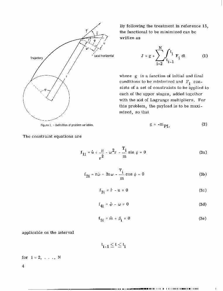
By following the treatment in reference 15, the functional to be minimized can be written as

Local hor izontal J = g + Tpi Fi dt (1 1 i=2 5-1

where g is a function of initial and final conditions to be minimized and F. con- s i s t s of a set of constraints to be applied to each of the upper stages, added together with the aid of Lagrange multipliers. For

1

this problem, the payload is to be maxi- mized, so that

PL Figure 1. - Definit ion of problem variables. g = -m

The constraint equations a r e

m

f2i = r& + 2uw - -cos Ti $ = 0 m

fgi = i- - u = 0

fqi = 6 - w = 0

fgi = m + p. = 0 1

applicable on the interval

t. < t < t . 1-1- - 1

for i = 2 , . . . , N

4

Equations (3a) to (3d) are the two-body equations of motion written in two-dimensional polar coordinates with an inverse square force field acting. The thrust direction q and the state variables are defined in figure 1. Equation (3e) defines the propellant flow rate.

Equations (3) a r e combined to give

i = 2 , . . . , N Fi = xj.f.. 1 J1 j =1

(4)

where h.. a r e undetermined Lagrange multipliers, which a r e functions of t ime since J1

the constraint equations must be satisfied at all points of the trajectory.

Eu I e r - Lag ra nge Equations

A s shown in reference 16, a necessary condition fo r g to be minimized is that the Euler -Lagrange equations be satisfied. The Euler -Lagrange equations a r e

where x a r e the problem variables j

7 X l ( t ) = u : x2(t) = w

x 3 ( t ) = r

x4(t) = (P

x5(t) = m

x6(t) = $

The Euler-Lagrange equations for the present problem can be written explicitly by use of equations (3) and (4):

5

x1 = 2wh2 - x3

U A4 x2 = - 2 9 + - A 2 - - r r

i3 = - (?+ W T x l + &A2

x4 = 0 (7d)

h5 = - (xl sin + + h2 cos +) 2 m

Equations (7) (and subsequent equations) apply separately to each of the upper stages. The subscript i has been omitted for simplicity.

Equation (7f) determines the thrust direction (for T f 0):

x1

h2 tan @ = -

h ,

x2 cos + = f dm The uncertainty in sign in equations (8b) and (8c) corresponds to an equivalent uncertainty of 180' in the thrust direction. ysis.

Equations (7a) to (7d) must be integrated, along with the equations of motion (eqs. (3a) to (3d)) to determine the thrust direction and the optimum trajectory. It is shown later that equation (7e) need not be integrated.

The choice of sign will be determined later in the anal-

Equation (7d) is easily integrated

6

to give

X4 = Constant (9)

First Integra I

Since the function F does not contain the independent variable (time) explicitly, a first integral to the Euler -Lagrange equations exists (for each stage), which can be stated as (ref. 16)

6

Equation (10) can be written explicitly by use of equations (3) and (4):

T m

C - - - w r x1 - 2uwx + uh3 + wx4 - px5 + - (xl sin q + x2 cos +) = 0 (11) (r' ") 2

Equation (11) is used later in the analysis to eliminate both C and X5 f rom the boundary equations.

We ie r st r as s Conditio n

The uncertainty in sign in equations (8b) and (8c) can be resolved by applying the necessary condition of Weierstrass (ref. 16). Following the development in reference 17, this condition can be stated as E > 0 for a minimum, where -

6 * aF xd a,, E = F ( J x * , x f ) J - F(x.,X.) J J -k (XT -

j =1 J

The x. correspond to the minimizing values, which differ from the x?; by a finite but J J

admissible amount. For the present problem, only Z/J is subject to such a variation. Equation (12) can be evaluated to give

7

I

T T m m

- - (xl sin $* + x2 cos $*) + - (xl sin + h2 cos +) > - o

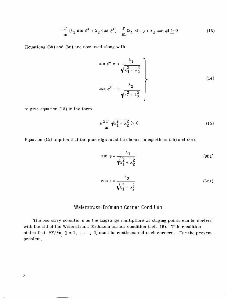
Equations (8b) and (8c) are now used along with

J x2 cos $*= T dm to give equation (13) in the form

V I L - m

Equation (15) implies that the plus sign must be chosen in equations (8b) and (8c).

1 sin $J =

h2 cos $J= dm

We i e r s t ra ss- Erd ma n n Cor n e r Co nd it ion

The boundary conditions on the Lagrange multipliers at staging points can be derived

For the present with the aid of the Weierstrass-Erdmann corner condition (ref. 16). This condition states that aF/& (j = 1, . . . , 6) must be continuous at such corners. problem,

J

8

I

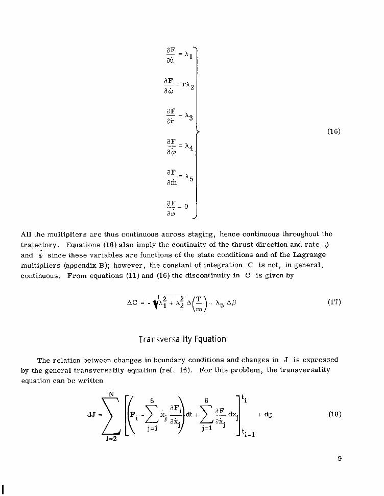
All the multipliers are thus continuous across staging, hence continuous throughout the trajectory. and $ since these variables a r e functions of the state conditions and of the Lagrange multipliers (appendix B); however, the constant of integration C is not, in general, continuous. From equations (11) and (16) the discontinuity in C is given by

Equations (16) also imply the continuity of the thrust direction and rate Z/J

AC = - X 1 + X 2 A - + A S A P d 2 (3 Transversal ity Equation

The relation between changes in boundary conditions and changes in J is expressed by the general transversality equation (ref. 16). equation can be written

For this problem, the transversality

d J =I i=2

(18)

9

I

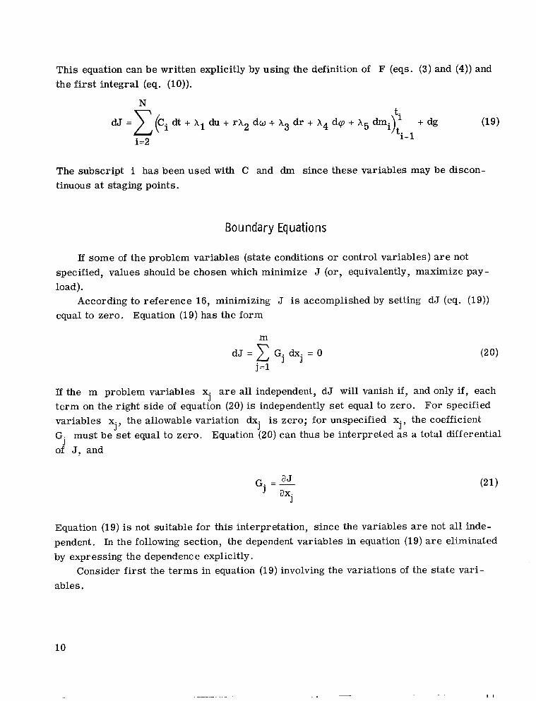
This equation can be written explicitly by using the definition of F (eqs. (3) and (4)) and the first integral (eq. (10)).

N

1-1 i=2

The subscript i has been used with C and d m since these variables may be discontinuous at staging points.

Boundary Equations

If some of the problem variables (state conditions o r control variables) are not specified, values should be chosen which minimize J (or, equivalently, maximize payload).

According to reference 16, minimizing J is accomplished by setting d J (eq. (19)) equal to zero. Equation (19) has the form

m

j =1 d J = G. dx. = 0

J J

If the m problem variables x te rm on the right side of equation (20) is independently se t equal to zero. For specified variables x., the allowable variation d x . is zero; for unspecified x. G. must be set equal to zero. Equation (20) can thus be interpreted as a total differential

J of J, and

are all independent, d J will vanish i f , and only i f , each j

the coefficient J J J’

Equation (19) is not suitable for this interpretation, since the variables a r e not all independent. In the following section, the dependent variables in equation (19) are eliminated by expressing the dependence explicitly.

ables. Consider first the t e r m s in equation (19) involving the variations of the state vari-

10

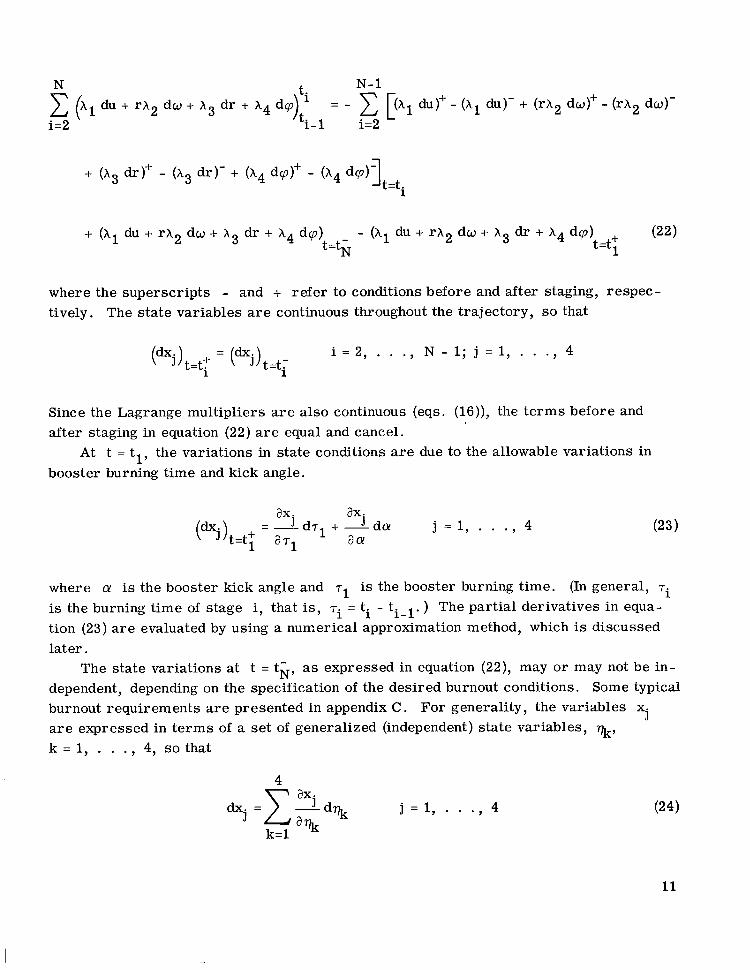
N- 1 5 (xl du + rh2 dw + X 3 d r + X d q): = - i=2 i-1 i=2

[(xl du)+ - (hl du)- + (rh2 dw)+ - (rX2 dw)-

+ (hl du + rx2 dw + x3 dr + x4 d q ) - - (A1 du + 'A2 dw + Ag d r + X4 d q ) t=tN t=tl +

(22)

where the superscripts - and + refer to conditions before and after staging, respectively. The state variables a r e continuous throughout the trajectory, so that

= d x i = 2 , . . ., N - 1 ; j = l , . . - 9 4 (dxj)t,t+ i ( j)t=t, 1

Since the Lagrange multipliers a r e also continuous (eqs. (16)), the t e rms before and after staging in equation (22) a r e equal and cancel.

booster burning t ime and kick angle. At t = tl, the variations in state conditions a r e due to the allowable variations in

ax ax

( j) t=t+ 1 aa dx - j - -dT1 + - j da! j = l , . . * , 4

where a! is the booster kick angle and T~ is the booster burning time. is the burning t ime of stage i, that is, T~ = ti - ti-l. ) The partial derivatives in equation (23) a r e evaluated by using a numerical approximation method, which is discussed later.

dependent, depending on the specification of the desired burnout conditions. Some typical burnout requirements a r e presented in appendix C. For generality, the variables x. J a r e expressed in t e r m s of a se t of generalized (independent) state variables, %, k = 1, . . . , 4, so that

(In general, T~

The state variations at t = t i , as expressed in equation (22), may or may not be in-

4

dx. J = c z d a j = 1 , . . ., 4

k = l

11

Equations (23) and (24) are combined with equation (22) to give

4 N (A1 du + r X 2 dw + X 3 dr + X4 =c (Al *+ r X 2 -+ aw X3 -+ ar x4 - a") dVj

'Vj 'Vj 'Vj a Vj j =1 t=tN i=2

+ rh2 e+ x3 - ar + ~4 2) dcy - fx1 * + rX2 -+ a m X3 - ar

a 0 act a c Y t=tl a T 1 a T1 a T1

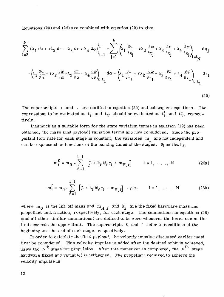
The superscripts + and - are omitted in equation (25) and subsequent equations. The expressions to be evaluated a t tl and tN should be evaluated at t; and tk, respectively.

Inasmuch as a suitable form for the state variation t e r m s in equation (19) has been obtained, the mass (and payload) variation t e rms are now considered. Since the propellant flow ra t e for each stage is constant, the variables mi are not independent and can be expressed as functions of the burning t imes of the stages. Specifically,

and kQ are the fixed hardware m a s s and H, Q

where mo is the lift-off m a s s and m propellant tank fraction, respectively, for each stage. The summations in equations (26) (and all other similar summations) are defined to be zero whenever the lower summation limit exceeds the upper limit. The superscripts 0 and f refer to conditions at the beginning and the end of each stage, respectively.

In order to calculate the final payload, the velocity impulse discussed earlier must f i r s t be considered. This velocity impulse is added after the desired orbit is achieved, using the Nth stage for propulsion. After this maneuver is completed, the Nth stage hardware (fixed and variable) is jettisoned. velocity impulse is

The propellant required to achieve the

12

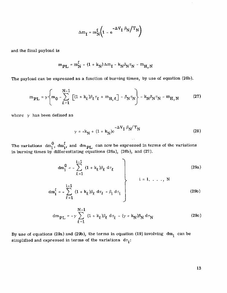
Am - m f ( 1 - e -Avl @NITN) I - N

and the final payload is

mpL = mN f - (1 + kN)AmI - k p T N N N - ~ H , N

The payload can be expressed as a function of burning times, by use of equation (26b).

where y has been defined as

-AvI f$J/TN y = -kN + (1 + kN)e

O f The variations dmi , dmi, and dmpL can now be expressed in t e rms of the variations in burning t imes by differentiating equations (26a), (26b), and (27).

i = l , . . ., N i-1

N-1

Q =1

By use of equations (29a) and (29b), the t e rms in equation (19) involving dmi can be simplified and expressed in t e rms of the variations dTi:

13

N L N N

N-1

i=2

N-1 N-1

where

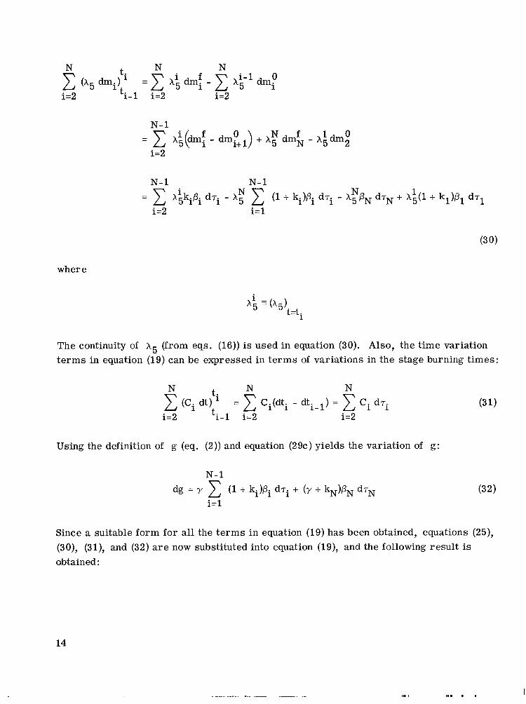
The continuity of h5 (from eqs. (16)) is used in equation (30). Also, the t ime variation t e rms in equation (19) can be expressed in t e rms of variations in the stage burning times:

N N N

i=2 ti-1 i=2 1=2 (Ci dt)t' = Ci(dti - dti-l) = C. 1 d 'i

Using the definition of g (eq. (2)) and equation (29c) yields the variation of g:

N-1

dg = Y (1 + ki)Pi dTi + ( y + kN)pN dTN i=l

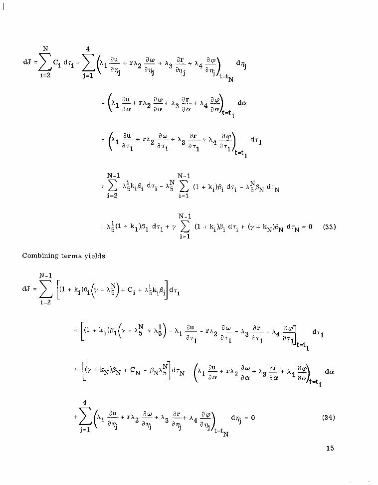
Since a suitable form for all the t e rms in equation (19) has been obtained, equations (25), (30), (31), and (32) are now substituted into equation (19), and the following result is obtained :

14

. . . .-

N 4

N-1

Combining t e r m s yields

N-1

d J = 2 El + ki)Pi (y - A:) + Ci + "kipi dTi 1 i=2

y - h; + h i ) - hl - au - r h 2 - a w -

a T1 a T1

(34)

15

I1 IIIII I IIIIIIII I I I

N The coefficient of dTi in equation (34) contains Ci and X 5 . Both of these can be elimi- N nated by using the following identity for X5 :

N N

N N N

_ - - -q5(Q - A;) + 2 (: - h:-1) + E (A; - *;-I) + A; (35)

Q =i+ 1 Q =i+ 1 Q =i+ 1 PQ+O PQ #' PQ =O

Equation (7e) shows that i, = 0 for coast phases, s o that for Ti = 0,

It is convenient to define

f s. = 0 1

0 s. = 0 1

i i-1 x5 = X 5

J pi = 0

pi = 0

- i = 2 , . . . , N

ar + x3 - aw

a 71

With these definitions, equation (3 5) becomes

16

h5 = - Q =i+ 1

By use of equations (37) and ( 3 8 ) , equation ( 3 4 ) becomes (if it is assumed that the first and last stages are powered):

N- 1 N

i=l Q =i+ 1

N-1

pi=O

4

dqj = 0 ar +Ctl *+ rx2 - aw + x3 -+ h4 a qj a Uj a Vj

j = l

(39)

The variations in equation (39) a r e all independent, so that the form of equation (20) has been achieved, with

G ( T ~ ) = Ci p. = 0- , i = 2 , . . . , N - 1

17

I

aw ar G ( q . ) = x1 - + r X 2 - + h3 - + X4 - J ( :", a Tj a Tj

-- w r X1 + 2uwx2 - ux3 - uh4 - -

From equations (11) and (37),

[(: - w2r)xl + 2uwx2 - ux3 - wx4 - 2 4 q i t=t i m

. ~ ___ - ~~~ - . f s; = 4 I

ci = [(: - "2')x1 + 2uwx2 - U h 3 - Olq] pi = 0;

pi#0; i = 2 , . . ., N

pi#O; i = 2 , . . ., N

t. < t < t i - 1 - - i

Since equations (41) do not contain C or X5, equation ("e) need not be integrated to evaluate equations (40), as indicated ear l ie r .

Boundary Value Problem

The determination of an optimum trajectory requires the simultaneous integration of the equations of motion (eqs. (3a) to (3d)) and the Euler-Lagrange equations (eqs. (7a) to (7d)). A set of initial conditions (state variables and Lagrange multipliers) and staging t imes is required in order to start the integration and to specify the trajectory uniquely.

the N + 5 independent problem variables in equation (39). For specified variables x the final conditions have the form

The trajectory thus generated must satisfy N + 5 final conditions, corresponding to

j '

x. = x J j , d

where the subscript d indicates the desired final value. For unspecified variables,

18

equations (40) supply auxiliary final conditions with the form

G(x.) = 0 (43) J

Some of equations (42) a r e easily satisfied; for example, a specified burning time for any stage can be achieved simply by terminating that stage at the proper time during the integration.

An iteration is required in order to satisfy the nontrivial final conditions, and variable initial conditions (equal to the number of final conditions) must be available. For the present problem, the initial state conditions cannot be varied independently, since these variables a r e determined by the choice of booster burning t ime and kick angle. The Lagrange multipliers (Ai, i = 1, . . . , 4), however, can be varied independently. In addition, the burning t imes of all stages being optimized and the booster kick angle (if it is being optimized) a r e available as variable initial conditions.

listed as follows: The initial and final conditions for the two-point boundary value problem can be

Unknown initial condition

7 “K

7 Desired final condition

j = 1 , . . . , 4

G ( a ) = 0

(i.1) = O

(7nK) = O

(44)

Equation (44) contains K + 5 unknown initial conditions (for K optimized stages, K < N) and an equal number of desired final conditions. The size of the iteration loop can be reduced by using the fact that equations (7) a r e homogeneous in the A ’ s . This implies that the choice of any one A in equation (44) is arbi t rary and serves only as a scale factor for the others. The value of this multiplier can be chosen to satisfy one of equations (40a) or (40c) appearing on the right side of equation (44). The choice of the arbi- t r a ry multiplier is made in appendix B.

-

19

I

l l 1 l 1 1 l l l I

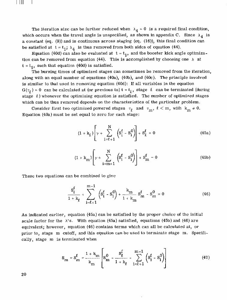
The iteration size can be further reduced when X4 = 0 is a required final condition, Since X 4 is which occurs when the travel angle is unspecified, as shown in appendix C.

a constant (eq. (9)) and is continuous across staging (eq. (16)), this final condition can be satisfied at t = tl; X4 is thus removed from both sides of equation (44).

tion can be removed from equation (44). This is accomplished by choosing one X at t = tl, such that equation (40d) is satisfied.

along with an equal number of equations (40a), (40b), and (40c). is s imilar to that used in removing equation (40d): If all variables in the equation G ( T ~ ) = 0 can be calculated at (or previous to) t = tQ, stage Q can be terminated (during stage Q ) whenever the optimizing equation is satisfied. The number of optimized stages which can be thus removed depends on the characteristics of the particular problem.

and T ~ , Q < m, with km # 0. Equation (40a) must be set equal to zero for each stage:

Equation (40d) can also be evaluated at t = tl, and the booster kick angle optimiza-

The burning t imes of optimized stages can sometimes be removed from the iteration, The principle involved

Consider first two optimized powered stages TQ

N

i=m+ 1

These two equations can be combined to give

c m-1

A s indicated earlier, equation (45a) can be satisfied by the proper choice of the initial scale factor for the A ' s . With equation (45a) satisfied, equations (45b) and (46) a r e equivalent; however, equation (46) contains te rms which can all be calculated at, or prior to, stage m cutoff, and this equation can be used to terminate stage m. Specifi- cally, stage m is terminated when

r

m-1 - c i=Q+1

(Sf - sf)] (47 )

20

. . ... . . ... __

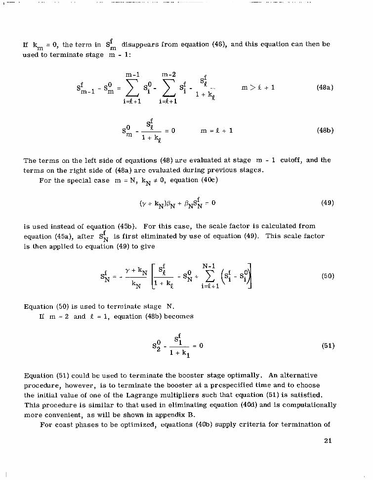
If km = 0, the te rm in S', disappears f rom equation (46), and this equation can then be used to terminate stage m - 1:

m-1 m-2 P

m > Q + l f 'm-1

i=Q + 1 i=Q+l

The te rms on the left side of equations (48) a r e evaluated at stage m - 1 cutoff, and the t e rms on the right side of (48a) a r e evaluated during previous stages.

For the special case m = N, kN # 0, equation ( 4 k )

is used instead of equation (45b). For this case, the scale factor is calculated from equation (45a), after SfN is first eliminated by use of equation (49). This scale factor is then applied to equation (49) to give

f y + k N sN=----

kN

[q s: 0 - SN +

Equation (50) is used to terminate stage N. If m = 2 and Q = 1, equation (48b) becomes

y i=Q+l

Equation (51) could be used to terminate the booster stage optimally. An alternative procedure, however, is to terminate the booster at a prespecified time and to choose the initial value of one of the Lagrange multipliers such that equation (51) is satisfied. This procedure is similar to that used in eliminating equation (4Od) and is computationally more convenient, as will be shown in appendix B.

For coast phases to be optimized, equations (40b) supply cri teria for termination of

21

the previous stage, similar to equations (48) and (51). For such cases, stage Q - 1 is terminated when CQ = 0, where stage Q is the coasting stage to be optimized.

In general, use of the preceding equations can supply either zero, one, or two equations for termination of a stage. If no equation is supplied, the burning time of that stage must be used as an initial condition in the external iteration. If one o r two equations for termination are available, the stage is terminated by u s e of one of the equations, and the additional equation (if available) is used as a desired final condition in the external iteration.

One other simplification of the two-point boundary value problem is possible when stage N is being optimized but cannot be terminated by use of equation (50) (this occurs when kN = 0). For this case, stage N can be terminated when one of the desired orbit conditions (appendix C) is satisfied; T~ and one of the orbit conditions a r e thus eliminated from equation (44). It is important, however, to choose an orbit condition which increases or decreases monotonically during flight, so that the desired value will always be achieved. Energy and velocity are two examples of such terminating variables.

Choice of Initial Conditions

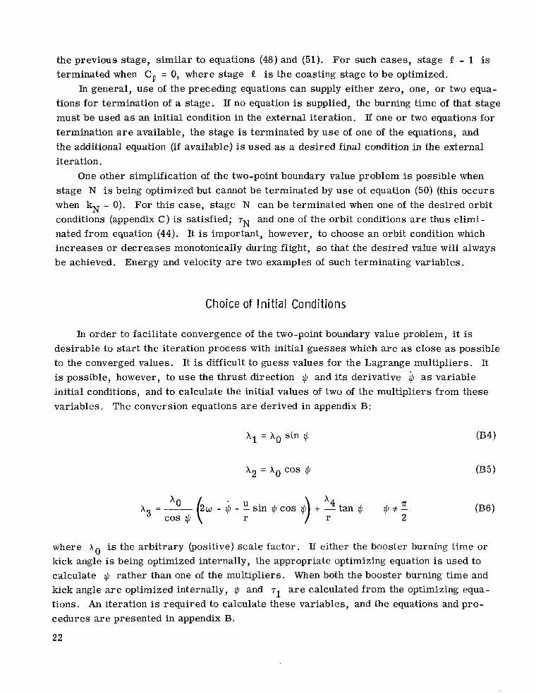
In order to facilitate convergence of the two-point boundary value problem, it is desirable to start the iteration process with initial guesses which are as close as possible to the converged values. It is difficult to guess values for the Lagrange multipliers. It is possible, however, to use the thrust direction + and its derivative $ as variable initial conditions, and to calculate the initial values of two of the multipliers from these variables. The conversion equations a r e derived in appendix B:

x2 = xo cos + 035)

036) ) ? 2 '0 2 w - + - - s i n + c o s + * u + - t a n + + + E L x3 =-

cos + where xo is the arbitrary (positive) scale factor. If either the booster burning time or kick angle is being optimized internally, the appropriate optimizing equation is used to calculate + rather than one of the multipliers. When both the booster burning time and kick angle are optimized internally, $ and T~ are calculated from the optimizing equations. An iteration is required to calculate these variables, and the equations and procedures a r e presented in appendix B.

22

Exa m p I es

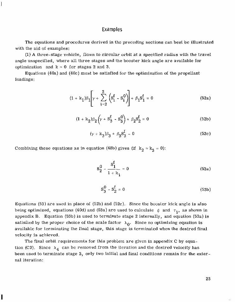
The equations and procedures derived in the preceding sections can best be illustrated

(1) A three-stage vehicle, flown to circular orbit a t a specified radius with the travel with the aid of examples:

angle unspecified, where all three stages and the booster kick angle are available for optimization and k = 0 for stages 2 and 3.

Equations (40a) and (40c) must be satisfied for the optimization of the propellant loadings:

Combining these equations as in equation (48b) gives (if k2 = k3 = 0):

0 s'l = o s2 - El

(53b) O f s3 - s2 = 0

Equations (53) a r e used in place of (52b) and (52c). Since the booster kick angle is also being optimized, equations (40d) and (53a) a r e used to calculate $ and T ~ , as shown in appendix B. Equation (53b) is used to terminate stage 2 internally, and equation (52a) is satisfied by the proper choice of the scale factor ho. Since no optimizing equation is available for terminating the final stage, this stage is terminated when the desired final velocity is achieved.

The final orbit requirements for this problem a r e given in appendix C by equation (C3). Since h4 can be removed from the iteration and the desired velocity has been used to terminate stage 3, only two initial and final conditions remain for the external iteration:

23

I I I I I I I I I I

1 Initial Final conditions conditions

i CY U = O J

(54)

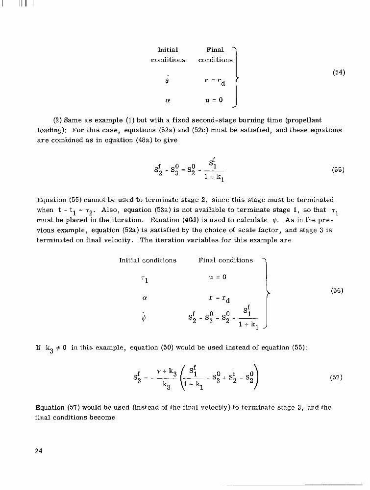
(2) Same as example (1) but with a fixed second-stage burning time (propellant loading): For this case, equations (52a) and (52c) must be satisfied, and these equations a r e combined as in equation (48a) to give

s 2 - s f O O - s s'l 3 - 2 - l + k l

(55)

Equation (55) cannot be used to terminate stage 2, since this stage must be terminated when t - tl = T ~ . Also, equation (53a) is not available to terminate stage 1, so that T~

must be placed in the iteration. Equation (4Od) is used to calculate $. As in the p re - vious example, equation (52a) is satisfied by the choice of scale factor, and stage 3 is terminated on final velocity. The iteration variables for this example a r e

7 Initial conditions Final conditions

T1

a!

s = s 0 0 s'l J s 2 - 3 2 - l + k 1 1

If k3 # 0 in this example, equation (50) would be used instead of equation (55):

O) s3 = - ~ (l+ - s3 + s2 - s2 f Y + k3 s'l O f

kg (57 1

Equation (57) would be used (instead of the final velocity) to terminate stage 3, and the final conditions become

24

u = o

d r = r

while the initial conditions remain the same as in equation (56).

PROCEDURE AND IMPLEMENTATION

In order to obtain numerical results, the equations derived in the preceding sections were programed for solution on an IBM 7094 computer. Equations (3) and (7) are integrated by using a variable step-size Runge-Kutta integration scheme with an e r r o r con- t ro l to minimize truncation effects (ref. 18).

variable Newton-Raphson iteration scheme. With this method, changes in final conditions are assumed to be related to changes in initial conditions by first-order, finite- difference equations:

The two-point boundary value problem of equation (44) is overcome by using a multi-

6Y = M 6X (59)

where 6X and 6Y are n-vectors (with an n x n iteration assumed) denoting differences in initial and final conditions, and M is an n x n matrix of partial derivatives of final conditions with respect to initial conditions :

The matrix M is obtained by integrating a reference trajectory and n independent perturbed trajectories, so that the equation

is obtained where AX is an n x n matrix of differences in initial conditions such that AXjk is the difference of the jth initial condition (from its value on the reference trajectory) on the k perturbed trajectory, and AY is an equivalent matrix of differences th

25

I

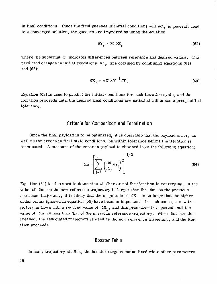
in final conditions. Since the first guesses of initial conditions will not, in general, lead to a converged solution, the guesses are improved by using the equation

where the subscript r indicates differences between reference and desired values. The predicted changes in initial conditions 6Xr are obtained by combining equations (61) and (62):

(63) 6Xr = A X AY-' 6Yr

Equation (63) is used to predict the initial conditions for each iteration cycle, and the iteration proceeds until the desired final conditions are satisfied within some prespecified tolerance.

Cr i te r ia for Comparison and Terminat ion

Since the final payload is to be optimized, it is desirable that the payload e r r o r , as well as the e r r o r s in final state conditions, be within tolerance before the iteration is terminated. A measure of the e r r o r in payload is obtained from the following equation:

Equation (64) is also used to determine whether or not the iteration is converging. If the value of 6m on the new reference trajectory is larger than the 6m on the previous reference trajectory, i t is likely that the magnitude of 6Xr is so large that the higher order t e r m s ignored in equation (59) have become important. In such cases, a new trajectory is flown with a reduced value of 6Xr, and this procedure is repeated until the value of 6m is less than that of the previous reference trajectory. When 6m has de- creased, the associated trajectory is used as the new reference trajectory, and the iteration proceeds.

Booster Table

In many trajectory studies, the booster stage remains fixed while other parameters

26

(such as upper-stage thrust levels and orbit parameters) are allowed to vary. Because of the large number of cases that can be run with the same booster stage, it is convenient to integrate a family of boost trajectories, and to s tore the burnout points in table form. The required booster burnout conditions can then be obtained from the table (by use of some interpolation scheme), rather than from an integration of new booster trajectories for each case. With lift-off thrust-to-weight ratio fixed, for example, two booster de- grees of freedom are available: kick angle and burning time. The booster table is thus a two parameter family of burnout points (radius, velocity, flight path angle, and weight).

For a problem involving a new booster stage, three booster trajectories are initially flown at different kick angles in the estimated region of interest. For each of these trajectories, the state variables are stored at fixed time intervals, ranging from minimum to maximum propellant loading. Other values of kick angle a r e flown and added to the table as required. During each computer run, the new booster data developed is stored and added to the table, so that after a series of computer runs using the same booster, a comprehensive table of booster burnout points is available.

A two-dimensional second-order interpolation scheme is used to determine the burnout conditions for intermediate values of kick angle and burning time. rivatives required in equations (40a) and (40d) are also determined, by differentiating the second-order interpolation polynomial. The interpolation accuracy depends on the table spacing as wel l as on the amount and form of variation between table points. In order to cover the region of interest with a minimum of trajectories, the initial kick angle spacing is large. On the other hand, t ime spacing is small, since only one trajectory is required to obtain a complete set of t ime points for each kick angle.

In order to determine whether or not the interpolation accuracy is acceptable, an additional booster trajectory is flown after convergence is achieved by using the converged values of burning time and kick angle. The upper stages are then reflown with the exact booster burnout conditions. The payload and burnout conditions from the exact flight a r e then compared with the resul ts of the interpolated converged flight. If agreement is acceptable, the interpolated resul ts a r e retained and the problem is finished. If agreement is not acceptable, new booster trajectories a r e flown and added to the table (in the region of convergence) by using valves of kick angle halfway between the previous table points. The flight is then reconverged with the modified table. The interpolation accuracy is tested as before, and the entire process is repeated (if necessary) until acceptable agreement is reached.

The partial de-

Convergence Propert ies

When the problem to be solved is not wel l known to the analyst, it is difficult to obtain initial conditions which are close to their converged values. On the other hand, the

27

equations for optimal staging a r e sometimes very strongly coupled to the initial conditions. For this reason, it is desirable to optimize the steering program and booster kick angle first, before attempting to optimize burning times.

For a three-stage vehicle to be completely optimized (booster kick angle and all three burning t imes optimized), the procedure is as follows: Firs t , the booster and second- stage burning t imes a r e held fixed at initial estimated values while the booster kick angle and third-stage burning time a r e optimized. The converged values of kick angle, pitch rate, and third-stage burning time a r e then used as f i rs t guesses, and the second- and third-stage burning times a r e optimized in the second case. Finally, all three stages (and the booster kick angle) a r e optimized in the third case.

This procedure has been used with good results in solving problems which were previously unfamiliar (as in the results presented). Of course, when the problem to be solved represents a small perturbation from a previously solved problem, complete optimization can be accomplished in one pass.

Perturbation S ize

A s discussed earlier, a finite difference procedure is used to obtain the partial derivatives of final conditions with respect to initial conditions. The perturbation sizes used for the initial conditions must be carefully selected: if the perturbations a r e too small, round-off and truncation e r r o r s inherent in the integration scheme cause large e r r o r s in the final differences; if the perturbations a r e too large, nonlinear effects become important, and incorrect local derivatives a r e obtained. The difficulty in choosing the proper perturbation sizes is magnified by the strong coupling of the partial derivatives to the optimal staging equations.

checking scheme was implemented in the program. With this scheme, the perturbation sizes a r e adjusted (when required) so that the payload e r r o r difference (eq. (64)) between reference and perturbed flights is between fixed limits. Generally, the perturbation sizes must be adjusted whenever the optimization cri teria a r e changed.

In order to obtain accurate local partial derivatives, an automatic perturbation size

RESULTS

In order to demonstrate the validity of the equations and the feasibility of the variational technique, parametric results a r e presented and compared with the overall optimum solutions obtained by using the variational technique. Two- and three-stage launch vehicles were optimized by use of the equations developed. The results presented include a two-stage vehicle flown to circular orbit and a three-stage vehicle flown to Earth escape

28

through a circular parking orbit. In these results, both fixed and variable hardware weights were used, and the propellant loadings and booster kick angle optimized. metr ic results a r e also presented, which show the variation of payload with propellant loadings and kick angle.

Para-

Vehicle Definition

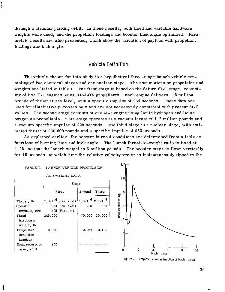
The vehicle chosen for this study is a hypothetical three-stage launch vehicle con- sisting of two chemical stages and one nuclear stage. The assumptions on propulsion and weights a r e listed in table I. The first stage is based on the Saturn SI-C stage, consist- ing of five F-1 engines using RP-LOX prdpellants. Each engine delivers 1. 5 million pounds of thrust at sea level, with a specific impulse of 264 seconds. These data a r e used for illustrative purposes only and a r e not necessarily consistent with present SI-C values. The second stage consists of one M-1 engine using liquid hydrogen and liquid oxygen as propellants. This stage operates at a vacuum thrust of 1. 5 million pounds and a vacuum specific impulse of 428 seconds. The third stage is a nuclear stage, with estimated thrust of 250 000 pounds and a specific impulse of 850 seconds.

A s explained earlier, the booster burnout conditions a r e determined from a table as functions of burning time and kick angle. The launch thrust-to-weight ratio is fixed at 1.25, so that the launch weight is 6 million pounds. The booster stage is flown vertically for 15 seconds, at which time the relative velocity vector is instantaneously tipped to the

TABLE I. - LAUNCH VEHICLE PROPULSION

Thrust, lb Specific

Fixed impulse, sec

hardware weight, lb

Propellant sensitive fraction

Drag reference area, s q f t

AND WEIGHT DATA

Stage

First

I . 5x106 (Sea level) 264 (Sea level) 305 (Vacuum)

!45,000

0.030

855

Second

1. 5X106 428

70,000

0.033

- - - - - - -

Third

5

850 i. 5x10

35,000

0.120

- - - - - - -

1 . 2 r

Mach number

Figure 2. - Drag coefficient as funct ion of Mach number.

29

I

I ' I I I 400 600 800 loo0 1200 1400 1 6 0 0 ~ 1 0 ~

Second-stage propellant loading, Ib

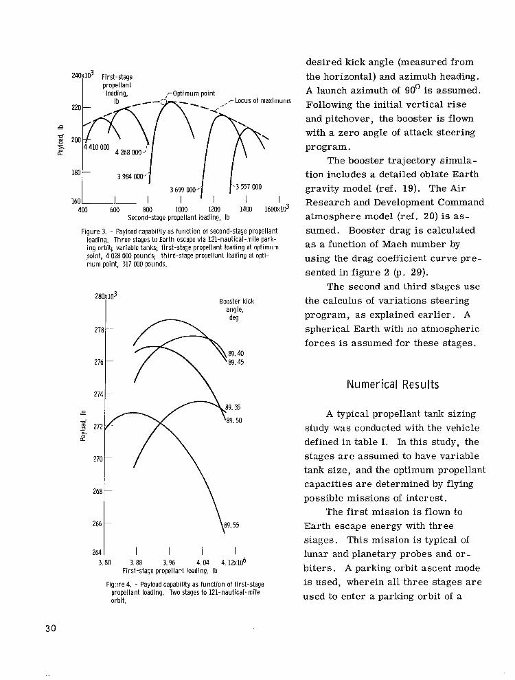
Figure 3. - Payload capability as funct ion of second-stage propellant loading. Three stages to Earth escape via 121-nautical-mile park- i ng orbit; variable tanks; first-stage propellant loading at optimum point, 4 028 000 pounds; third-stage propellant loading at optimum point, 317 000 pounds.

Booster kick angle.

P -0- m 0 x - 2

desired kick angle (measured from the horizontal) and azimuth heading. A launch azimuth of 90' is assumed. Following the initial vertical rise and pitchover, the booster is flown with a zero angle of attack steering program.

The booster trajectory simula- tion includes a detailed oblate Earth gravity model (ref. 19). The Air Research and Development Command atmosphere model (ref. 20) is assumed. Booster drag is calculated as a function of Mach number by using the drag coefficient curve p re - sented in figure 2 (p. 29).

The second and third stages use the calculus of variations steering program, as explained earlier. A spherical Earth with no atmospheric forces is assumed for these stages.

Nu mer ical Results

A typical propellant tank sizing study was conducted with the vehicle defined in table I. In this study, the stages are assumed to have variable tank size, and the optimum propellant capacities a r e determined by flying possible missions of interest.

Earth escape energy with three stages. This mission is typical of lunar and planetary probes and or - biters. A parking orbit ascent mode is used, wherein all three stages a r e used to enter a parking orbit of a

The first mission is flown to

30

280x103

m a

274

272 89.30

cop t imum point

I I I 89.35 89.40 89.45 89.50 89.55 89.60

Booster kick angle, deg

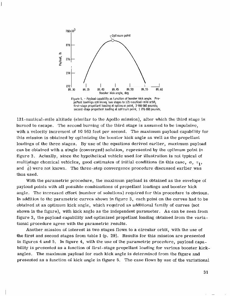
pellant loadings optimized; two stages to 121-nautical-mile orbit; first-stage propellant loading at optimum point, 3 980 000 pounds; second-stage propellant loading at optimum point, 1 276 OOO pounds.

Figure 5. - Payload capability as function of booster kick angle. Pro-

121-nautical-mile altitude (similar to the Apollo mission), after which the third stage is burned to escape. The second burning of the third stage is assumed to be impulsive, with a velocity increment of 10 563 feet per second. The maximum payload capability for this mission is obtained by optimizing the booster kick angle as well as the propellant loadings of the three stages. By use of the equations derived earlier, maximum payload can be obtained with a single (converged) solution, represented by the optimum point in figure 3 . Actually, since the hypothetical vehicle used fo r illustration is not typical of multistage chemical vehicles, good estimates of initial conditions (in this case, a, T ~ ,

and z)) were not known. The three-step convergence procedure discussed earlier was thus used.

payload points with all possible combinations of propellant loadings and booster kick angle. The increased effort (number of solutions) required for this procedure is obvious. In addition to the parametric curves shown in figure 3 , each point on the curves had to be obtained a t an optimum kick angle, which required an additional family of curves (not shown in the figure), with kick angle as the independent parameter. As can be seen from figure 3 , the payload capability and optimized propellant loading obtained from the variational procedure agree with the parametric results.

the first and second stages from table I (p. 29). Results for this mission are presented in figures 4 and 5. In figure 4, with the use of the parametric procedure, payload capability is presented as a function of first-stage propellant loading for various booster kick- angles. The maximum payload for each kick angle is determined from the figure and presented as a function of kick angle in figure 5. The case flown by use of the variational

U’ith the parametric procedure, the maximum payload is obtained as the envelope of

Another mission of interest is two stages flown to a circular orbit, with the use of

31

Fir st-stage propellant loading, ,-Optimum point

r Locus of

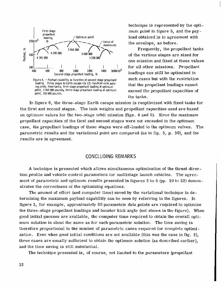
Figure 6. - Payload capability as funct ion of second-stage propellant loading. Three stages to Earth escape via 121-nautical-mile park- i ng orbit; fixed tanks; first-stage propellant loading at optimum point, 3 964 000 pounds; third-stage propellant loading at optimum point, 310 000 pounds.

technique is represented by the optimum point in figure 5, and the payload obtained is in agreement with the envelope, as before.

Frequently, the propellant tanks of the various stages are sized for one mission and fixed at these values for all other missions. Propellant loadings can still be optimized in such cases but with the restriction that the propellant loadings cannot exceed the propellant capacities of the tanks.

In figure 6 , the three-stage Earth escape mission is reoptimized with fixed tanks for the first and second stages. The tank weights and propellant capacities used a r e based on optimum values for the two-stage orbit mission (figs. 4 and 5). Since the maximum propellant capacities of the first and second stages were not exceeded in the optimum case, the propellant loadings of these stages were off -loaded to the optimum valves. The parametric results and the variational point a r e compared (as in fig. 3, p. 30), and the results a r e in agreement.

CONCLUDING REMARKS

A technique is presented which allows simultaneous optimization of the thrust direc - tion profile and vehicle control parameters for multistage launch vehicles. The agreement of parametric and optimum results presented in figures 3 to 6 (pp. 30 to 32) demon- s t ra tes the correctness of the optimizing equations.

The amount of effort (and computer time) saved by the variational technique in de- termining the maximum payload capability can be seen by referr ing to the figures. In figure 3, for example, approximately 80 parametric data points a r e required to optimize the three-stage propellant loadings and booster kick angle (not shown in the figure). When good initial guesses a r e available, the computer time required to obtain the overall optimum solution is about the same as for each parametric solution. The time saving is therefore proportional to the number of parametric cases required for complete optimization. Even when good initial conditions a r e not available (this was the case in fig. 3), three cases a r e usually sufficient to obtain the optimum solution (as described earlier) , and the t ime saving is still substantial.

The technique presented is, of course, not limited to the parameters (propellant

32

loadings and booster kick angle) used herein. Other possible parameters (for launch vehicle optimization problems) a r e launch thrust-to-weight ratio and thrust levels for the various stages. In addition, the technique should be applicable to other types of optimization problems.

Lewis Research Center, National Aeronautics and Space Administration,

Cleveland, Ohio, October 8, 1965.

33

I " " ' I "

APPENDIX A

SYMBOLS

a

b

C

E

e

F

f

G

g

H

J

k

M

m

P

r

S

T

t

U

V

X

functions defined in eqs. (BlO), a! booster kick angle, r ad

mass flow rate, slug/sec ft/ sec

sq ft / (sec2)(rad) I' flight path angle, r ad

y

E argument of perigee, rad

generalized state variable

functions defined in eqs. (B13),

function defined in eq. (28) constant of integration

Weiers t rass excess function

eccentricity 5 8 t rue anomaly, rad 5: hjfj

j =I constraint equation

aJ/ ax

h Lagrange multiplier

X o arbitrary scale factor

p 2 Earth force constant, cu ft/sec

7 burning time, sec function of initial and final conditions to be minimized cp polar angle, rad

2 zc) thrust direction, rad energy per unit mass , s q ft/sec

functional to be minimized by varia- o angular velocity, rad/sec

Subscripts :

d desired value

tional methods

propellant sensitive mass fraction

matrix relating changes in final and initial conditions

mass, slugs

semilatus rectum, f t

radius, f t

functions defined in eqs. (37)

thrust, lb

time, sec

radial velocity, ft/sec

velocity, ft/sec

problem variable

H

I

i

j

k

Q

N

PL

P

r

fixed hardware

impulsive

stage number

variable number

variable number

stage number

last stage

payload

propellant

difference between reference and desired values

34

s structure

0 initial

Superscripts:

f end of stage

i r e fe r s to t = t.

0 beginning of stage 1

- *

derivative with respect to time

finite, but allowable variation of the variable

+ after staging

- before staging

-. vector

35

APPENDIX B

CONVERSION EQUATIONS

Ca I c u I at ion of Lag ra ng e Mu It i p I i er s

In order to avoid the difficulty associated with guessing initial values of the Lagrange multipliers, equations a r e derived which express two of the multipliers in t e rms of the pitch attitude $ and r a t e i.

Equations (8a), (8b1) and (8cl) give $ in t e r m s of the Lagrange multipliers:

x1

x2 tan $ = -

x, 1 sin $ =

x2 cos 11, = {m Differentiating equation (8a) yields the pitch rate

- 2 x2x1 - v 2 $sec $ =

which becomes, with the use of equations (8cl), (?a), and (7b),

The discussion following equation (44) shows that one of the multipliers can be picked arbitrarily. It is convenient to pick hO as the scale factor, where

36

ho = dm> 0 With this choice,

XI = ho sin +

x2 = xo cos +

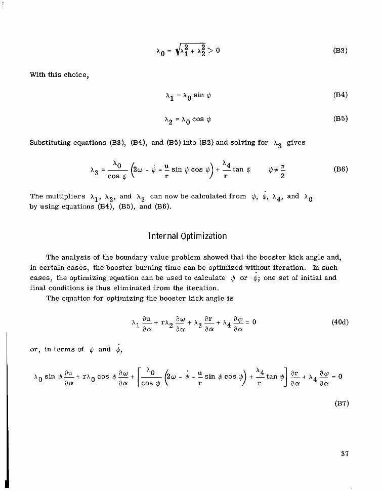
Substituting equations (B3), (B4), and (B5) into (B2) and solving for X3 gives

- U - s i n + c o s + + + E 2

h3 =- cos + r

The multipliers X1, h2, and X3 can now be calculated from +, +, h4, and ho

by using equations (B4), (B5), and (B6).

1 nter na l Opt imizat ion

The analysis of the boundary value problem showed that the booster kick angle and, in certain cases, the booster burning time can be optimized without iteration. In such cases , the optimizing equation can be used to calculate z) or +; one set of initial and final conditions is thus eliminated from the iteration.

The equation for optimizing the booster kick angle is

x ~ - + ~ x ~ * + x ~ - + x ~ + = o au ar aa aa aa aa

or , in t e rms of z,b and $,

- u 2w - + - - s i n + c o s 1 ~ , +- tan + -+ x X sin z,b -+ r X cos + -+ ~

aq - o aw [c::+ ( r : 1:: 4aa!-

au aa a 0 0 0

37

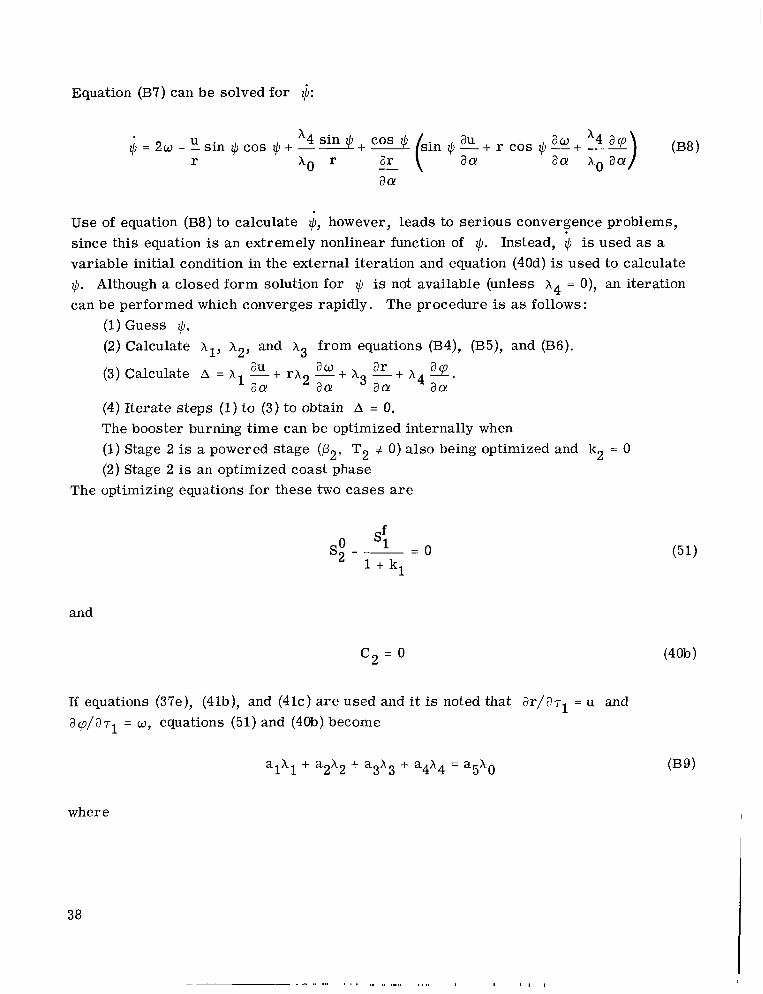
Equation (B7) can be solved for 4:

Use of equation (B8) to calculate $, however, leads to ser ious convergence problems, since this equation is an extremely nonlinear function of $. Instead, zl, is used as a variable initial condition in the external iteration and equation (40d) is used to calculate $. Although a closed form solution for $J is not available (unless X4 = 0), an iteration can be performed which converges rapidly. The procedure is as follows:

(1)Guess q. (2) Calculate X1, x2, and X3 f rom equations (B4), (B5), and (B6).

(3) Calculate A = X1 - + r X 2 - + X3 - + X4

(4) Iterate steps (1) to (3) to obtain A = 0. The booster burning time can be optimized internally when (1) Stage 2 is a powered stage (p2, T2 # 0) also being optimized and k2 = 0 (2) Stage 2 is an optimized coast phase

The optimizing equations for these two cases a r e

ar *. au a m a 0 a 0 a 0 a 0

0 Sf - 0 S 2 - l + k l -

and

c2 = 0

If equations (37e), (41b), and (41c) a r e used and i t is noted that a r / aT1 = u and a p / a ~ ~ = w, equations (51) and (40b) become

a X + a X + a X + a4X4 = a5XO 1 1 2 2 3 3

where

38

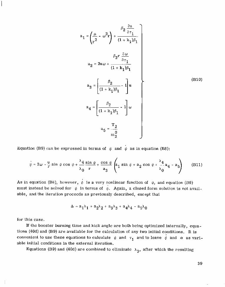
P

a5 =o "2

Equation (B9) can be expressed in t e rms of z,b and z,b as in equation (B8):

(B11) ''sin + + * I4 sin + a2 cos + + -a XO

z,b=2w--sin$~cos$+----- . U r

Xo I- a3

As in equation (B8), however, $ is a very nonlinear function of $, and equation (B9) must instead be solved for z,b in t e rms of $. Again, a closed form solution is not available, and the iteration proceeds as previously described, except that

A = alXl + a X + a X + a4h4 - ash0 2 2 3 3

for this case.

tions (40d) and (B9) are available for the calculation of any two initial conditions. It is convenient to use these equations to calculate z,b and T~ and to leave $ and CY as var i - able initial conditions in the external iteration.

Equations (B9) and (40d) are combined to eliminate X3, after which the resulting

If the booster burning t ime and kick angle are both being optimized internally, equa-

39

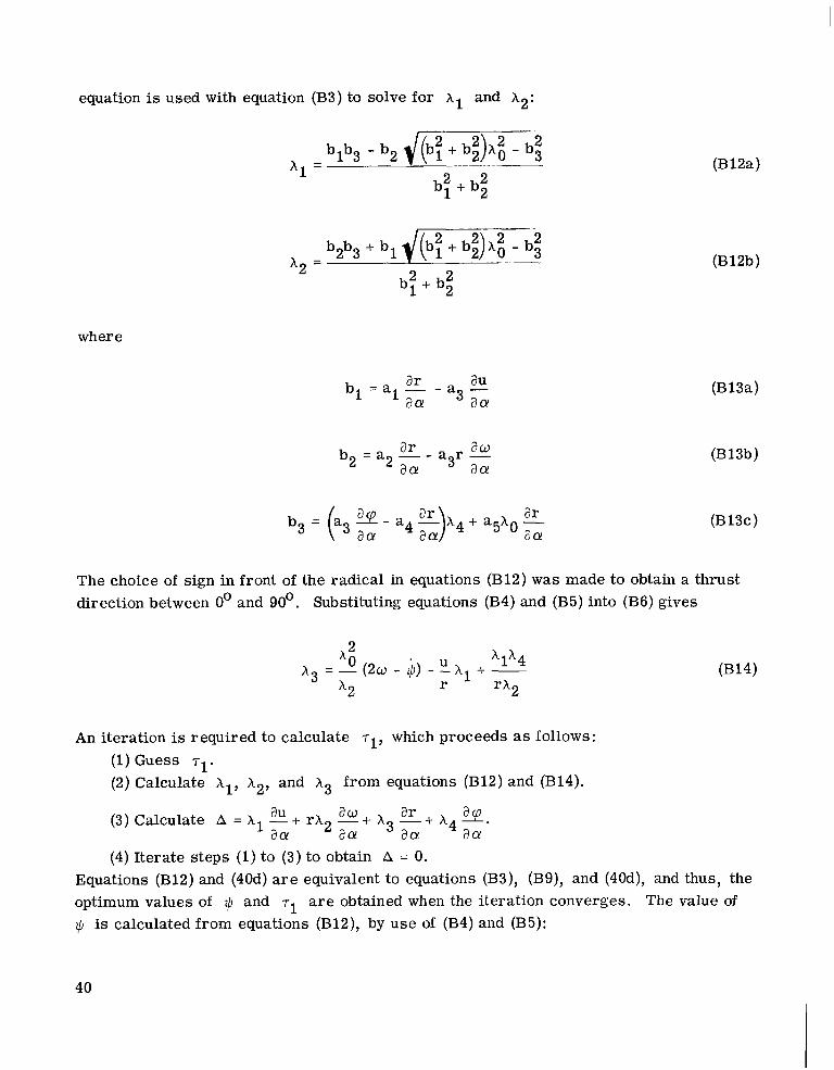
equation is used with equation (B3) to solve for X1 and h2:

1 2 2 bl + b2

b2b3 + b l {(b: + b2)ho 2 2 - b i x, =

2 2 bl + b2

L

where

The choice of sign in front of the radical in equations direction between 0' and 90'. Substituting equations

,2

(B12a)

(B12b)

(B13a)

(B 13b)

(B13c)

(B12) was made to obtain a thrust (B4) and (B5) into (B6) gives

*O * u '1'4 x3 = - (2w - $) - 4 1 + - r rh2 x2

An iteration is required to calculate T ~ , which proceeds as follows: (1) Guess T ~ .

(2) Calculate X1, h2, and X3 from equations (B12) and (B14).

au a # ar a 0 aa act aa

(3) Calculate A = x1 -+ rx2 -+ x3 -+ x4 *. (4) Iterate steps (1) to (3) to obtain A = 0.

Equations (B12) and (40d) a r e equivalent to equations (B3), (B9), and (40d), and thus, the optimum values of z) and T~ a r e obtained when the iteration converges. The value of z) is calculated from equations (B12), by use of (B4) and (B5):

40

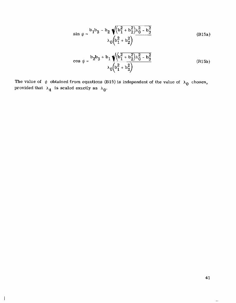
b2b3 + bl {(b: + b2)Ao 2 2 - bt cos 11, =

(B 15a)

(B15b)

The value of 11, obtained from equations (B15) is independent of the value of Xo chosen, provided that x4 is scaled exactly as xo.

41

APPENDIX C

0 R B IT R EQU I R EMENTS

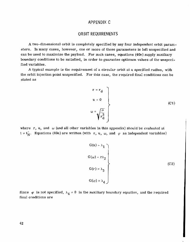
A two-dimensional orbit is completely specified by any four independent orbit param- e te rs . In many cases, however, one or more of these parameters is left unspecified and can be used to maximize the payload. For such cases, equations (40e) supply auxiliary boundary conditions to be satisfied, in order to guarantee optimum values of the unspecified variables.

the orbit injection point unspecified. stated as

A typical example is the requirement of a circular orbit at a specified radius, with For this case, the required final conditions can be

u = o I where r, u, and w (and all other variables in this appendix) should be evaluated at t = t i . Equations (40e) a r e written (with r, u, w, and q~ as independent variables)

Since 40 is not specified, X 4 = 0 is the auxiliary boundary equation, and the required final conditions a r e

42

w=fi

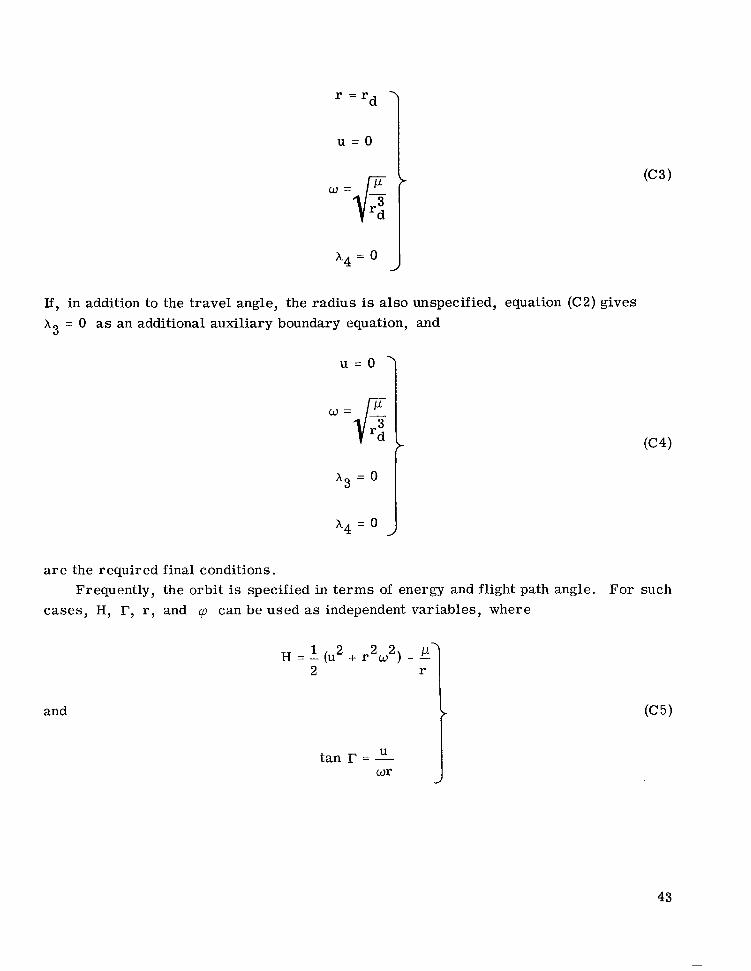
u = o t J A 4 = 0

If, in addition to the travel angle, the radius is also unspecified, equation (C2) gives X 3 = 0 as an additional auxiliary boundary equation, and

w:i; x3 = 0

x4 = 0 J are the required final conditions.

cases, H, r, r , and cp can be used as independent variables, where Frequently, the orbit is specified in t e rms of energy and flight path angle. For such

1 2 2

H = - ( U +

and

tan r U - _ - w r

43

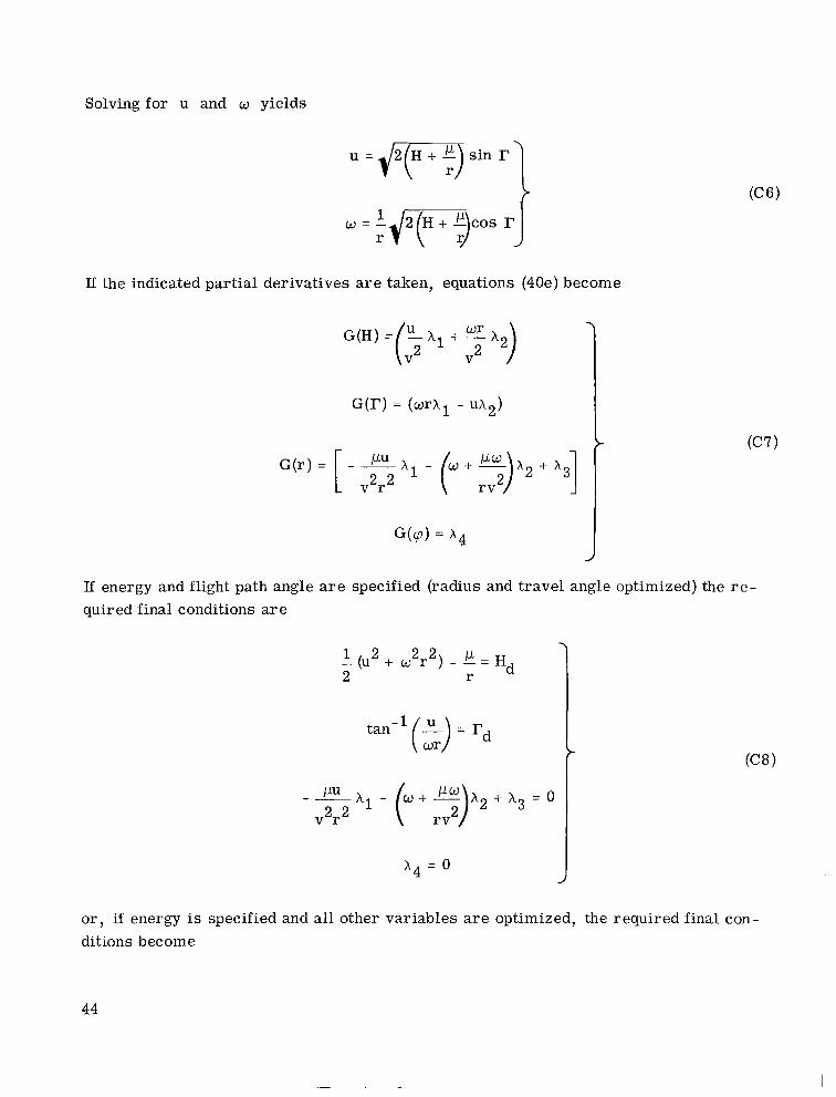
Solving for u and o yields

u = , / W s i n r)

If the indicated partial derivatives are taken, equations (40e) become

V

G ( r ) = (wrX1 - uh2)

G ( d = A4

If energy and flight path angle a r e specified (radius and travel angle optimized) the r e - quir ed final conditions ar e

1 1 2 2 2 2 r d -(u + ~ ~ ) - I J - = H

- - PU 2 2 h l - ( w + 3 X 2 + X 3 = 0 v r

X 4 = 0 J or, if energy is specified and all other variables are optimized, the required final conditions become

44

1 2 2 2 -(u + r ~ ) - L = H 2 r d

- - PU X I - (w + $)A2 + XR = 0

v r

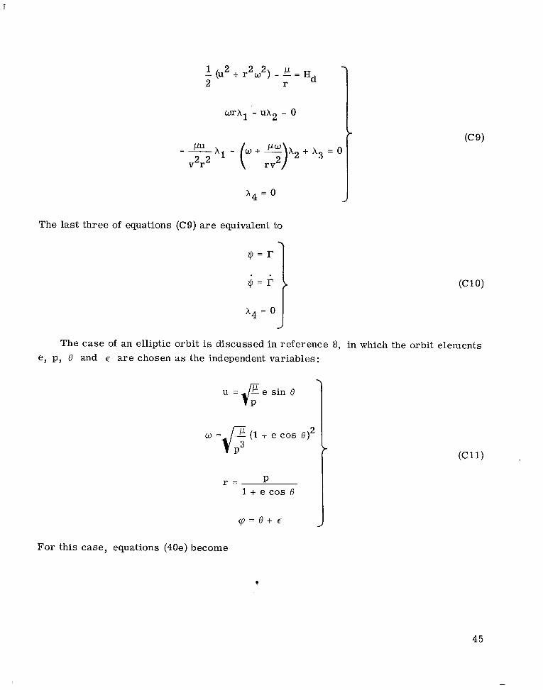
X4 = 0 J The last three of equations (C9) are equivalent to

x4 :::) = 0

The case of an elliptic orbit is discussed in reference 8, in which the orbit elements e, p, 0 and E a r e chosen as the independent variables:

1 u =Ee sin 0

J 1 + e cos 0

q = 0 + €

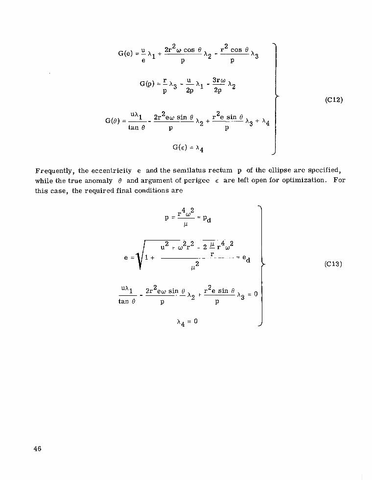
For this case, equations (40e) become

?

45

A3 I 2 r cos 0 2 2 r w COS 8 G(e) = EAl + A2 - e P

r U 3r w G(p)=-X3- -A1- - x2

P 2P 2P

2 A3 + x4

r e sin 0

P uA1 2r 2 e o sin e

A2 + G(8) = -- tan 0 P

G(E) = A 4 J Frequently, the eccentricity e and the semilatus rectum p of the ellipse a r e specified, while the t rue anomaly 8 and argument of perigee E a r e left open for optimization. For this case, the required final conditions a r e

A 4 = 0

46

REFERENCES

1. Goldsmith, M. : On the Optimization of Two-Stage Rockets. J e t Prop. , vol. 27, no. 4, Apr. 1957, pp. 415-416.

2 . Schurmann, Ernest E . H. : Optimum Staging Technique for Multistaged Rocket Ve- hicles. Je t Prop. , vol. 27, no. 8, Aug. 1957, pp. 863-865.

3 . Subotowicz, M. : The Optimization of the N-Step Rocket with Different Construction Parameters and Propellant Specific Impulses in Each Stage. Jet Prop . , vol. 28, no. 7, July 1958, pp. 460-463.

4 . Hall, H. H. ; and Zambelli, E . D. : On the Optimization of Multistage Rockets. Jet Prop. , vol. 28, no. 7, July 1958, pp. 463-465.

5 . Weisbord, L . : Optimum Staging Techniques. J e t Prop. , vol. 29, no. 6, June 1959, pp. 445-446.

6 . Cobb, Edgar R. : Optimum Staging Technique to Maximize Payload Total Energy. ARS J . , vol. 31, no. 3, Mar. 1961, pp. 342-344.

7. Coleman, John J. : Optimum Stage-Weight Distribution of Multistage Rockets. ARS J., vol. 31, no. 2, Feb. 1961, pp. 259-261.

8 . Zimmerman, Arthur V. ; MacKay, John S. ; and Rossa, Leonard G. : Optimum Low- Acceleration Trajectories for Interplanetary Transfers . NASA TN D-1456, 1963.

9. Melbourne, William G. ; and Sauer, Car l G . , Jr. : Optimum Thrust Programs for Power-Limited Propulsion Systems. C . I . T . , June 15, 1961.

Rept. No. TR 32-118, Je t Prop. Lab. ,

10. MacKay, John S . ; and Rossa, Leonard G. : A Variational Method for the Optimiza- tion of Interplanetary Round-Trip Trajectories. NASA TN D-1660, 1963.

11. Jurovics, Stephen: Optimum Steering Program for the Entry of a Multistage Vehicle into a Circular Orbit. ARS J., vol. 31, no. 4, Apr. 1961, pp. 518-522.

12. Mason, J. D. ; Dickerson, W. D. ; and Smith, D. B. : A Variational Method for Opti- mal Staging. No. 65-62, AIAA, Jan. 1965.

Paper presented at ALAA 2nd Aerospace Sciences Meeting, Paper

13. Denbow, C.H. : Generalized Form of the Problem of Bolza. Ph.D. Thesis, Univ. of Chicago, 1937.

14. Hunt, R. W. ; and Andrus, J. F. : Optimization of Trajector ies having Discontinuous Paper Presented at SUM State Variables and Intermediate Boundary Conditions.

Meeting, Monterey, (Calif. ), Jan. 1964.

47

15. Stancil, R. T. ; and Kulakowski, L . J. : Rocket Boost Vehicle Mission Optimization. ARS J., vol. 31, no. 7, July 1961, pp. 935-942.

16. Bliss, G.A. : Lectures on the Calculus of Variations. Univ. Chicago P res s , 1946.

17. Leitmann, G. : On a Class of Variational Problems in Rocket Flight. J. Aero/Space Sci., vol. 26, no. 9, Sept. 1959, pp. 586-591.

18. Strack, William C. ; and Huff, Vearl N. : The N-Body Code - A General Fortran Code for the Numerical Solution of Space Mechanics Problems on an IBM 7090 Computer. NASA T N D-1730, 1963.

19. Clarke, Victor C . , Jr. : Constants and Related Data for Use in Trajectory Calcula- tions as Adopted by the Ad Hoc NASA Standard Constants Committee. NASA CR-53921, 1964.

20. Minzner, R.A. ; Champion, K. S. W. ; and Pond, N. L. : The ARDC Model Atmosphere, 1959. Air Force Surveys in Geophysics No. 115, Rept. No. TR-59-267, Air Force Cambridge Res. Center, Aug. 1959.

48 NASA-Langley, 1966 E-3154

. . . .. . . . . . - ,

" T h e aeronautical m d space activities of the United States shall be conducted so as to contribute . . . t o the expansioii of humaiz KiiowI- edge of phenomena in the atmosphere and space. T h e Administration shall provide for the widest practicable and appropriate dissemination of information concerning its actiuities and the results thereof .'I

-NATIONAL AERONAUTICS A N D SPACE ACT OF 1958

NASA SCIENTIFIC A N D TECHNICAL PUBLICATIONS

TECHNICAL REPORTS: important, complete, and a lasting contribution to existing knowledge.

TECHNICAL NOTES: of importance as a contribution to existing knowledge.

TECHNICAL MEMORANDUMS: Information receiving limited distribution because of preliminary data, security classification, or other reasons.

CONTRACTOR REPORTS: Technical information generated in con- nection with a NASA contract or grant and released under NASA auspices.

TECHNICAL TRANSLATIONS: Information published in a foreign language considered to merit NASA distribution in English.

TECHNICAL REPRINTS: Information derived from NASA activities and initially published in the form of journal articles.

SPECIAL PUBLICATIONS: Information derived from or of value to NASA activities but not necessarily reporting the results .of individual NASA-programmed scientific efforts, Publications include conference proceedings, monographs, data compilations, handbooks, sourcebooks, and special bibliographies.

Scientific and technical information considered

Information less broad in scope but nevertheless

Details on the availability of these publications may be obtained from:

SCIENTIFIC AND TECHNICAL INFORMATION DIVISION

N AT1 0 N A L A E R O N A U T I CS A N D SPACE A D M I N I ST R A T 1 0 N

Washington, D.C. 20546

Documents

Payload optimization of multistage launch vehicles · payload optimization of multistage launch vehicles ~ ... payload optimization of multistage launch vehicles ... x2 = -29 + u