Embed Size (px)
Citation preview

Biological Journal of the Linnean Society (2001), 73: 345–390. With 15 figures
doi:10.1006/bijl.2001.0542, available online at http://www.idealibrary.com on
Patterns of animal dispersal, vicariance anddiversification in the Holarctic
ISABEL SANMARTIN1∗, HENRIK ENGHOFF2 and FREDRIK RONQUIST1
1Department of Systematic Zoology, Evolutionary Biology Centre, Uppsala University, Norbyvagen 18D,SE-752 36 Uppsala, Sweden2Zoologisk Museum, Universitetsparken 15, DK-2100 Copenhagen, Denmark
Received 23 October 2000; accepted for publication 25 March 2001
We analysed patterns of animal dispersal, vicariance and diversification in the Holarctic based on completephylogenies of 57 extant non-marine taxa, together comprising 770 species, documenting biogeographic events fromthe Late Mesozoic to the present. Four major areas, each corresponding to a historically persistent landmass, wereused in the analyses: eastern Nearctic (EN), western Nearctic (WN), eastern Palaeoarctic (EP) and westernPalaeoarctic (WP). Parsimony-based tree fitting showed that there is no significantly supported general areacladogram for the dataset. Yet, distributions are strongly phylogenetically conserved, as revealed by dispersal-vicariance analysis (DIVA). DIVA-based permutation tests were used to pinpoint phylogenetically determinedbiogeographic patterns. Consistent with expectations, continental dispersals (WP↔EP and WN↔EN) are sig-nificantly more common than palaeocontinental dispersals (WN↔EP and EN↔WP), which in turn are more commonthan disjunct dispersals (EN↔EP and WN↔WP). There is significant dispersal asymmetry both within the Nearctic(WN→EN more common than EN→WN) and the Palaeoarctic (EP→WP more common than WP→EP). Cross-Beringian faunal connections have traditionally been emphasized but are not more important than cross-Atlanticconnections in our data set. To analyse changes over time, we sorted biogeographic events into four major timeperiods using fossil, biogeographic and molecular evidence combined with a ‘branching clock’. These analyses showthat trans-Atlantic distributions (EN–WP) were common in the Early–Mid Tertiary (70–20 Myr), whereas trans-Beringian distributions (WN–EP) were rare in that period. Most EN–EP disjunctions date back to the Early Tertiary(70–45 Myr), suggesting that they resulted from division of cross-Atlantic rather than cross-Beringian distributions.Diversification in WN and WP increased in the Quaternary (< 3 Myr), whereas in EP and EN it decreased from amaximum in the Early–Mid Tertiary. 2001 The Linnean Society of London
ADDITIONAL KEY WORDS: historical biogeography – trans-Atlantic – trans-Beringian – disjunct.
This incongruence is measured in abstract terms, suchINTRODUCTIONas items of error or amount of homoplasy. The in-
The surge of phylogenetic systematics in recent dec- congruence can then be interpreted a posteriori inades has created an increased interest in phylogeny- terms of biogeographic events, such as dispersal andbased biogeographic analyses. However, beyond the extinction. The exact procedure for this a posteriorifact that such analyses should be based on robust translation remains elusive. Furthermore, because nophylogenies of many groups of organisms with well- model is specified, it is difficult to predict the analyticalknown distributions, there is currently little agree- behaviour of pattern-based methods and counter-in-ment concerning methodology. The existing approaches tuitive results often occur (e.g. Ronquist, 1995, 1996).can be roughly characterized as being event-based or In contrast, event-based methods are explicitly de-pattern-based (Ronquist, 1997, 1998a). Pattern-based rived from models of biogeographic processes. Themethods explicitly avoid making assumptions about relevant events are identified and associated with costsevolutionary processes. The analyses identify patterns, that are inversely related to the likelihood of thewhich typically show some incongruence with the data. events. The analysis consists of a search for the re-
construction, which minimizes the total cost. Thisoptimal reconstruction explicitly specifies the bio-geographic events of interest, unlike pattern-based∗Corresponding author. E-mail: [email protected]
3450024–4066/01/080345+46 $35.00/0 2001 The Linnean Society of London
346 I. SANMARTIN ET AL.
analyses, and no a posteriori interpretation is neces- and eastern North America. The extinction in othersary. The direct relation between method, model and areas is attributed to a combination of climatic andevent–cost assignments makes it easy to understand geological changes during the Late Tertiary–the properties of an event-based method. For these Quaternary (Tiffney, 1985b).reasons, we apply the event-based approach in this The eastern North America–Asia disjunction haspaper. been documented in a long series of plant taxa but
Phylogenetic biogeographic studies often focus solely there is still considerable controversy surrounding theon hierarchical patterns (area cladograms) and rarely processes that created it and only a few studies havetest the significance of the resultant patterns. However, documented the pattern phylogenetically (Wen, 1999).there is no theory predicting a prevalence of hier- Estimates of divergence times based on the moleculararchical patterns in historical biogeography. We believe clock suggest that this disjunct pattern evolved mul-that biogeographers should be more open-minded in tiple times (polychronically) in the Tertiary (Wen,their search for patterns and more critical in evaluating 1999). The disjunction has thus far only been dem-their results by using significance tests or other pro- onstrated in a few animal groups (Suzuki et al., 1977;cedures for assessing uncertainty. By analysing each Patterson, 1981; Andersen & Spence, 1992; Enghoff,individual group separately before looking for general 1993; Nordlander, Liu & Ronquist, 1996; Savage &patterns, we have a better chance of finding multiple, Wheeler, 1999) and there is uncertainty concerningincongruent histories than if the data set is reduced its general importance in the evolution of Holarcticto a single dominant area cladogram (Noonan, 1988a). faunas.
Phylogeny-associated age estimates, whether de- Another familiar Holarctic pattern is the unequalrived from morphological or molecular clock estimates, distribution of species diversity among infraregions,fossil data or external biogeographic events, provide which has been extensively documented for temperatecritical information in phylogenetic biogeographic plant species (Latham & Ricklefs, 1993; Qian & Rick-studies. For instance, age estimates are essential in lefs, 1999, 2000). These authors discussed the causaluntangling pseudocongruence, that is, similar patterns factors creating this pattern in the Tertiary using dataof different age (Cunningham & Collins, 1994). There- from fossil floras and simulated rarefaction of extantfore, we believe that phylogenetic biogeographers floras. However, their analyses were based on tra-should include age estimates, even if they are un- ditional classifications and did not include explicitcertain, in their analyses. phylogenetic information. Several additional studies
In this paper, we present a comprehensive event- of Holarctic plant biogeography could be mentionedbased analysis of biogeographic patterns in the Hol- but, to our knowledge, general Holarctic patterns havearctic following the principles outlined above. still not been documented in a large set of plant phylo-
genies.There have been several studies of the biogeographic
HOLARCTIC BIOGEOGRAPHY history of the Holarctic fauna (Allen, 1983; Noonan,1988a,b; Enghoff, 1993, 1995; De Jong, 1998) but mostThe southern Hemisphere has been a favourite regionof them cover only one or two of the Holarctic infra-for historical biogeographic studies. One reason forregions. Enghoff (1995) is the only comprehensivethis is the presence of many widely disjunct but closelystudy of the entire Holarctic. It was based on phylo-related taxa on the southern continents, spurring in-genies of 73 extant non-marine Holarctic animalterest in biogeographic processes. Another reason isgroups. The phylogenies were divided into two groups:the relatively simple geological history of the Southernfamily clades (for groups at the family level or above)continents (but see Seberg, 1991 for a different view).and genus clades (for groups at the genus level orIn contrast, large-scale Holarctic distribution patternsbelow). The former were presumed to document olderare less obvious and palaeogeographic reconstructionsevents than the latter, but dating of the clades wassuggest a more complicated history. Nevertheless,never attempted. Patterns were analysed in terms ofsome patterns have attracted considerable attention.four major areas (‘infraregions’): western North Amer-The best example is perhaps the striking similarityica (WN), eastern North America (EN), western Pa-between the floras of eastern Asia and eastern Northlaeoarctic (WP) and eastern Palaeoarctic (EP). UsingAmerica (Gray, 1840; Li, 1952; Tiffney, 1985a,b; Wolfe,pattern-based methods, Enghoff (1995) found a strong1969, 1975, 1985; Xiang, Soltis & Soltis, 1998a; Xianghierarchical pattern in the genus clades reflecting theet al., 1998b; Wen, 1999). The much cited boreotropicscurrent continental configuration: ((WN, EN), (WP,hypothesis (Wolfe, 1985; Tiffney, 1985a) explains thisEP)). However, the significance of this result was notdisjunction as the result of the fragmentation of atested and it contrasts with recent palaeogeographiconce continuous warm–temperate forest that extendedreconstructions, indicating that the Late Mesozoic andacross the Northern Hemisphere during the Early–Mid
Tertiary, leaving extant remnants only in eastern Asia Cenozoic biogeographic history of the Holarctic follows

HOLARCTIC BIOGEOGRAPHY 347
a reticulate scenario (Smith, Smith & Funnell, 1994).Enghoff (1995) also analysed ancestral areas of eachgroup and the frequency of different types of dispersalevents. Unfortunately, only one of the dispersal pat-terns was tested statistically and this test was biasedbecause it did not correct for differences in speciesrichness among infraregions. Furthermore, none ofthese analyses was explicitly event-based.
Here we present a considerably more detailed ana-lysis of Holarctic biogeographic patterns. We as-sembled published phylogenies of 57 non-marineanimal groups occurring mainly or exlusively in theHolarctic. In contrast to Enghoff (1995), we only in-cluded phylogenies that were resolved down to thespecies level and which included a complete or almostcomplete sample of the species in the group. Age es-timates suggest that the phylogenies in our data setdocument events from the Late Mesozoic to the present.In total, the phylogenies comprised 770 extant speciesconnected by 713 lineage splitting (speciation) events.In analysing the data set, we consistently used event-based methods, searched both for hierarchical andreticulate patterns, and tested the significance of ourresults using permutation tests designed specificallyto reveal phylogenetically constrained biogeographicpatterns. In some analyses, the ages of all nodes wereestimated using various methods to allow tracking ofpatterns through time.
Figure 1. Palaeogeographic reconstruction of the North-SETTING THE SCENARIOern Hemisphere in the Late Jurassic (150 Myr) modified
To provide a basis for the discussion of biogeographic from Barron et al. (1981). Stereographic projection. Emer-hypotheses pertaining to the Holarctic, we provide a gent land is shaded by grey and major mountain chainsbrief summary of current reconstructions of the history by dark grey. Current coastlines are indicated by thinof this region from the Mesozoic to the present (Figs lines. Abbreviations: UMt=Ural Mountains.1–4).
Early Mesozoic: Pangaea (Cox, 1974; Raven &Axelrod, 1974) Late Mesozoic: Euramerica–Asiamerica (Cox, 1974;
Tiffney, 1985a)During the Triassic (200 million years ago (Myr)), allpresent continents formed a single landmass, Pangaea. In the Mid–Late Cretaceous (100–80 Myr), epi-Splitting of Pangaea started in the Early–Mid Jurassic continental seaways and intercontinental connections(180 Myr) with the division into a northern continent, divided Laurasia into two palaeocontinents:Laurasia, comprising North America and Eurasia, and Euramerica and Asiamerica. Europe and easterna southern continent, Gondwana. North America (Euramerica) were still linked across
The major Laurasian landmasses, the eastern and the Atlantic, whereas Asia and western North Americawestern Nearctic and the eastern and western Pal- (Asiamerica) became connected by the Bering landaeoarctic, were joined to each other in various com- bridge. Two epicontinental seaways separatedbinations over time. In the Early Jurassic, Europe Euramerica and Asiamerica: the Turgai Strait throughand North America were connected through the proto- central Asia and eastern Europe, and the Mid-Con-British Isles, which acted as a big ‘stepping-stone’ in tinental Seaway through central North America (Fig.the middle of a narrow Atlantic ocean (Smith et al., 2). This continental arrangement lasted around 25–301994). North America and Asia, however, were widely Myr, disintegrating at the end of the Cretaceous–Earlyseparated. This situation persisted through the Late Palaeocene (70–65 Myr) with the closing of the Mid-
Continental Seaway.Jurassic (Fig. 1).

348 I. SANMARTIN ET AL.
A more northern trans-Atlantic connection, the DeGeer Bridge, persisted until the Late Eocene. It con-nected Scandinavia (Fennoscandia) to northern Green-land, and Greenland to eastern North America throughthe Canadian Arctic Archipelago. This route is con-sidered far less important for biotic exchange thanthe Thulean Bridge because of its northern position,restricting it to cold-adapted organisms. Furthermore,Scandinavia was isolated from direct contact withEurope by the Danish–Polish trough through much ofthe Palaeogene. The Greenland Sea broke this north-ern route in the Late Eocene (39 Myr). A third con-nection between Europe and eastern North America,the Greenland–Faeroes bridge, probably persisteduntil the Miocene but this connection was apparentlynever more than a chain of islands, and is not con-sidered to have been an important dispersal route.
Trans-Beringian land bridges (Mathews, 1979;McKenna, 1983; Lafontaine & Wood, 1988;Tangelder, 1988; Nordlander et al., 1996)
Asia and Western North America became connectedby land across the Bering Sea in the Mid Cretaceous(100 Myr). The continents remained joined by theBering land bridge until the Pliocene. The Beringiantransgression opened the Bering Strait in the LatePliocene (3.5 Myr) but the land connection was re-established several times during the Pleistocene (e.g.during the Illinoisan and Wisconsinan glaciations).Figure 2. Palaeogeographic reconstruction of the North-
The climatic and floristic conditions prevailing onern Hemisphere in the Late Cretaceous (80 Myr). Majorthe Beringian land bridge changed considerably oversource, projection and symbols as in Figure 1. Ab-time. Thus, the importance of Beringia as a dispersalbreviations: MCS=Mid-Continental Seaway, TS=Turgairoute is likely to have varied considerably over time.Sea.Three consecutive phases with different climate andvegetation in the Beringian area may be recognized.Trans-Atlantic land bridges (McKenna, 1983; Tiffney,
1985a,b; Liebherr, 1991)
The opening of the North Atlantic started in the Late Beringian Bridge I. During the Early Tertiary, aftersome climatic fluctuations in the Palaeocene followingCretaceous (90 Myr) but terrestrial connections be-
tween Europe and North America persisted along vari- the impact winter that ended the Cretaceous, climatesin the Northern Hemisphere became much warmerous North Atlantic land bridges until at least the Early
Eocene (50 Myr). Three different North Atlantic land and humid than they are today (the Early Eocenewarming event). A continuous belt of vegetation, thebridges, geographically and temporally separated,
have been postulated (McKenna, 1983; Tiffney, 1985b). boreotropical forest, is considered to have extendedover the entire Northern Hemisphere during thisDuring the Early Tertiary, the Thulean Bridge is
supposed to have connected southern Europe to Green- period, from Asia through North America across Ber-ingia (Wolfe, 1969, 1975, 1978). The boreotropical forestland through the British Isles. Greenland, in turn,
was connected westwards with eastern North America consisted of a mixture of deciduous hardwoods andevergreen subtropical elements (Wolfe, 1985). De-through the Queen Elizabeth Islands (Fig. 3). The
Thulean Bridge is considered to have been the most ciduous plants were rare in the Late Cretaceous butthe impact winter at the KT boundary (65 Myr) mayimportant route for exchange of temperate biota in the
earliest part of the Early Eocene (55 Myr), when the have promoted their rise to dominance in Early Ter-tiary forests (Wolfe, 1987). The origin of the boreo-climate became markedly warmer (McKenna, 1983).
This interchange was suddenly interrupted with the tropical forest is associated with the evolution of alarge number of modern plant taxa in the latest Cre-breaking of the Thulean Bridge in the Early Eocene
(50 Myr). taceous and Early Tertiary. The new plants spread

HOLARCTIC BIOGEOGRAPHY 349
rapidly over existing land bridges, ultimately forming Asia and North America were re-established. A con-tinuous tree-less steppe, the tundra, then connecteda homogeneous flora. During this period, considerable
exchange of terrestrial fauna and flora is thought Siberia with Alaska across Beringia. The tundra hab-itat acted as a barrier to mixing of taiga species,to have occurred across the Beringian land bridge,
predominantly in species adapted to warm-temperate separating the Nearctic and Palaeoarctic portions ofthe boreal forest during the Pleistocene. During thisclimates and associated with the boreotropical forest
(Tiffney, 1985a). period, trans-Beringian biotic exchange was probablyAt the Eocene–Oligocene boundary (35 Myr), there dominated by arctic, tundra-adapted groups. Dispersal
was a drastic and global decline in climatic conditions, was eventually interrupted in the Late Pleistocene–which became cooler and drier (the terminal Eocene Holocene, with the retreat of the ice-sheets and theevent). This resulted in the demise of the boreotropical final marine transgression of the Bering area. Tundraforest and subsequent trans-Beringian isolation and species are still much the same on both sides of thevicariance in the organisms living in the forest. The Bering strait (Pielou, 1979; Lafontaine & Wood, 1988).boreotropical forest was replaced by the mixed meso-phytic forest (Wolfe, 1987), a mixed deciduous hardwood
The Nearctic (Allen, 1983; Tiffney, 1985b; Noonan,and coniferous forest, which became dominant in the1986, 1988a; Tangelder, 1988; Askevold, 1991)mid-Tertiary. Although faunal exchange of cold–
temperate groups across Beringia probably continued In the mid Cretaceous (100 Myr), the Mid-Continentalin the Oligocene and Miocene (Tiffney, 1985a), most Seaway, located to the east of the Rocky Mountains,dispersal of temperate groups across Beringia is con- completely divided the North American continent intosidered to have stopped after the terminal Eocene an eastern and a western half from the Gulf of Mexicoevent, marking the end of Beringian Bridge I. to the Canadian Arctic Archipelago (Fig. 2). The seaway
partially retreated in the Late Cretaceous (84 Myr),allowing connections in the north, and finally dis-Beringian Bridge II. As climates continued to de-appeared at the end of the Cretaceous (70 Myr). Thisteriorate during the Miocene, the Beringian forestwas presumably followed by an Early Cenozoic periodbecame successively more dominated by coniferousof floral and faunal exchange between the eastern andelements. From the Middle–Late Miocene (14–10 Myr)western Nearctic. However, the disappearance of theto the Late Pliocene (3.5 Myr), a continuous coniferousMid-Continental seaway was concurrent with the up-forest belt connected northern Asia with northernlift of the Cordilleran Mountain System in the LateNorth America across Beringia. The forest was similarCretaceous: the Rocky Mountains and the Sierrain composition to the present taiga but with the sameMadre Occidental (Fig. 3). As they rose, the Rockyconifer species occurring in both Siberia and NorthMountains cast an increasingly large rain shadow toAmerica. During this period, trans-Beringian dispersalthe east. By the Late Eocene (35 Myr), this had createdwas presumably dominated by boreal elements, whilea dry-habitat barrier between the western and easternwarm–temperate groups were restricted to widely dis-Nearctic, even though migration corridors with wetterjunct refugia in the south (Lafontaine & Wood, 1988).habitats persisted along rivers. The Eocene–OligoceneFurther deterioration of climatic conditions duringclimatic deterioration resulted in the contraction ofthe Pliocene and Pleistocene resulted in vicariance ofthe original boreotropical flora in the western moun-the boreal coniferous forest into an eastern and atains and in the eastern part of North America, andwestern portion. The division was reinforced in thein the geographical expansion of temperate deciduousLate Pliocene (3.5 Myr), when a marine transgressionelements in the mixed-mesophytic forest. By the Oli-opened the Bering Strait and broke the terrestrialgocene (30 Myr), erosion had completely wiped out theconnections between America and Asia. Palaeoarcticearly Rocky Mountains and the entire Cordilleranand Nearctic forests have never come into contact since.range became a peneplain. This presumably enabledThese climatic, geographic and vegetational changesa second Cenozoic period of extensive dispersal be-assumedly resulted in massive trans-Beringian vicar-tween the western and eastern sides of the Nearctic.iance in boreal groups, which is reflected by the high
In the Late Oligocene (25 Myr), and continuing inproportion of Nearctic–Palaeoarctic species pairs inthe Miocene, a new orogenic phase gave rise to thethe taiga fauna (Lafontaine & Wood, 1988). Today, allpresent western Cordilleran System, including newspecies of conifers, and most other tree species as well,folding of the Rocky Mountains and Sierra Madreare different on the Siberian and Alaskan sides ofOccidental and the uplift of Sierra Madre OrientalBeringia (Pielou, 1979; Lafontaine & Wood, 1988).(Fig. 4). This resulted in cooler and drier climates and,eventually, in the development of grassland biomes incentral North America. The new topographic barrierBeringian Bridge III. During the Pleistocene gla-
ciations (1.5–1.0 Myr), terrestrial connections between definitively divided the western and eastern sides of

350 I. SANMARTIN ET AL.
Figure 4. Palaeogeographic reconstruction of the North-Figure 3. Palaeogeographic reconstruction of the North-ern Hemisphere in the Late Tertiary (20 Myr). Majorern Hemisphere in the Early Tertiary (50 Myr). Majorsource, projection, and symbols as in Figure 1. Ab-source, projection, and symbols as in Figure 1. Ab-breviations: RMt=Rocky Mountains, UMt=Ural Moun-breviations: DG=‘De Geer’ North-Atlantic bridge, RMt-tains.Rocky Mountains, TH=‘Thulean’ North-Atlantic bridge,
TS=Turgai Sea.
along the coasts and islands of the Tethys Seaway(Tiffney, 1985b). Temporary regression of the Turgaithe mixed-mesophytic forest and was presumably as-Sea in the Palaeocene allowed connections in the northsociated with massive vicariance in Nearctic biotas.but they were interrupted by a new transgression inThe mesophytic elements became restricted to easternthe Eocene. The Turgai Strait finally dried up duringNorth America and the west side of the Rocky Moun-the Oligocene (30 Myr), permitting extensive biotictains, while a more drought-tolerant, temperate de-exchange between both sides of the Palaeoarctic (Fig.ciduous flora evolved in the western mountains4). The closing of the Turgai Strait introduced a more(Tiffney, 1985b). Finally, the last remnants of thecontinental climate in western Siberia. This led to themixed-mesophytic forest were wiped out from westernevolution of increasingly drought-tolerant, deciduousNorth America during the Pleistocene glaciations.communities of plants, which ultimately invaded Eur-ope from the east, replacing the mixed-mesophytic
The Palaeoarctic (Cox, 1974; Tiffney, 1985b; forest. The last remnants of the latter forest becameTangelder, 1988) extinct in Europe during the Quaternary glaciations
(Tiffney, 1985b).From the Mid-Jurassic (180 Myr) to the Late Tertiary(30 Myr), the Palaeoarctic was divided into an eastern Several partial barriers between the two sides of the
Palaeoarctic appeared after the Turgai Strait dried up.and a western half by an epicontinental seaway, theTurgai Strait, located at the east of the Ural Mountains In the Late Oligocene, the uplift of the Tibet Mountains
isolated Europe and West Asia from East Asia (Macey(Figs 1–3). However, some authors argue that floral andfaunal exchange between Europe and Asia persisted et al., 1999). During the Late Pliocene–Pleistocene,

HOLARCTIC BIOGEOGRAPHY 351
exchange between Asia and Europe was interrupted isolated western and eastern North America, floraland faunal exchange should have been more frequentseveral times because of climatic fluctuations, which
periodically reinforced the West-Siberian dry con- in the Nearctic than in the Palaeoarctic. Enghoff’s(1995) pattern-based analysis supported this pre-tinental climate barrier (Beschovski, 1984). Opening
of the Japanese Sea, which resulted in the vicariance diction weakly, but the significance of the result wasnot tested.between Japanese and Asian biotas, started in the
Miocene but did not completely isolate the Japanese Although there is no obvious geological evidence forislands until the Late Miocene–Early Pliocene (6 Myr). dispersal asymmetries in the Palaeoarctic, EnghoffThe Himalayan Mountains were formed by the collision (1995) found that dispersals from the eastern to theof India with Asia in the Middle Eocene, with the most western Palaeoarctic were more common than dis-intense orogenic phase occurring in the mid-Miocene persals in the other direction. Again, the significance(15 Myr) (Tangelder, 1988). of this result was not tested. This is problematic since
the extant fauna of most groups of organisms is con-siderably more diverse in the eastern than in theBIOGEOGRAPHIC HYPOTHESESwestern Palaeoarctic. Thus, by pure chance one wouldBased on the current views on the history of theexpect extant faunas to document more dispersalHolarctic, reviewed above, we extracted the followingevents from the east to the west than in the otherhypotheses and ideas that we wanted to test.direction. We re-examined Enghoff’s results, correctingfor such diversity differences.A general area cladogram for the Holarctic?
The Tertiary orogenic activity in the western Ne-Although the palaeogeographic history of the four Hol- arctic presumably created cold and dry adapted formsarctic infraregions since the Late Mesozoic cannot that later became successful in the eastern Nearcticeasily be summarized in a general area cladogram, when climates in general deteriorated towards the endEnghoff (1995), using pattern-based methods (com- of the Tertiary and in the Quaternary. In addition, theponent analysis), found considerable support for the dry continental climates of interior North America firstarea cladogram ((WN, EN), (WP, EP)) in his genus originated close to the Rocky Mountains and thenphylogenies. However, the statistical significance of spread east as the mountains rose. Therefore, Tertiarythis result was not tested. To clarify whether Holarctic and Quaternary dispersal in the Nearctic should havebiogeography can be adequately summarized in a gen- been predominantly from the west to the east. Theeral area cladogram, we searched for such patterns role of western North America as a source area ofboth in Enghoff’s and our own data using event-based continental dispersal is consistent with the presencemethods and permutation tests to assess the sig- there of many relict forms and a high proportion ofnificance of the results. endemic taxa (Shear & Gruber, 1983; Kavanaugh,
1988). Enghoff’s (1995) analyses indicated pre-Large-scale Holarctic patterns dominantly eastwards dispersal in the Nearctic, butHolarctic geographic history combined with the effects the statistical significance of this asymmetry was notof extinction and diversification predict that, among tested. Here, we address this hypothesis.the events documented in phylogenies of extant or-ganisms, continental dispersals (within the present
Trans-Beringian and trans-Atlantic exchangelandmasses North America and Eurasia, WN↔EN andWP↔EP) should be more frequent than palaeo- Nearctic–Palaeoarctic disjunctions have usually beencontinental dispersals (trans-Beringian and trans-At- explained as being derived from ancestral distributionlantic dispersals, WN↔EP and EN↔WP), which in ranges extending across the Bering land bridge (Dar-turn should be more frequent than disjunct dispersals lington, 1957). However, recent studies suggest thatbetween infraregions that have never been directly trans-Atlantic dispersal may have played a more im-connected (EN↔EP, WN↔WP). Enghoff (1995), using portant role in this type of disjunction than is com-cladistic subordinateness as an indicator of dispersal monly assumed (Tiffney, 1985b; Noonan, 1986, 1988b).(Enghoff, 1993), found a pattern consistent with this Trans-Beringian dispersal is presumed to have beenexpectation but he did not correct for the effects of more frequent from the eastern Palaeoarctic to westernregional differences in species diversity, nor did he North America than in the other direction, at leastuse explicit event-based methods in identifying the during the Pleistocene (Pielou, 1979). The reason isdispersals. that, during full-glacial periods, Beringia was es-
sentially an eastward extension of Siberia. The landContinental patterns covered with ice was more extensive in western North
America than in Asia and the unglaciated parts ofBecause the Turgai Sea divided the Palaeoarctic for amuch longer time than the Mid-Continental Seaway Alaska and Yukon were separated from the rest of
352 I. SANMARTIN ET AL.
North America by the Laurentide and Cordilleran ice- most of Europe and advanced deeply into eastern NorthAmerica (Pielou, 1979). Glaciation and the associatedsheets. Thus, only a small portion of the Americanclimatic cooling were supposedly associated with highfauna could access Beringian Bridge III. Beringia isextinction rates. In Asia, however, the ice neverconsidered to have contributed the bulk of tundrareached as far south and, in addition, the Asian faunaspecies that now range across northern North America,and flora could disperse freely into the warmer habitatswhereas forest and prairie species from non-Beringianof the Oriental region. Thus, thermophilic taxa thatareas of North America made little or no contributionwent extinct elsewhere survived in Asia, resulting into the present fauna of Siberia (George, 1988; Lafon-the high extant diversity of Asian faunas and florastaine & Wood, 1988). We tested whether this predicted(Tiffney, 1985a).directional asymmetry was evident in our data.
The diversification hypothesis assumes that the di-versity asymmetries arose already in the Tertiary,
The eastern North America–Asia disjunctionbefore the climatic cooling and widespread extirpations
Although well known in plants, this disjunction has of the Quaternary. The richness of the Asian flora andrarely been documented in animals (but see Suzuki et fauna would have resulted because the net di-al., 1977; Patterson, 1981; Andersen & Spence, 1992; versification rates were higher in Asia than in otherEnghoff, 1993; Nordlander et al., 1996; Savage & Holarctic infraregions during the Tertiary (Latham &Wheeler, 1999). However, the boreotropics hypothesis Ricklefs, 1993; Nordlander et al., 1996; Qian & Ricklefs,predicts that this pattern should be common in animals 1999, 2000). We tested these hypotheses with our datedassociated with warm-temperate forests of boreo- phylogenies.tropical origin, in which case the pattern should becommon in our data set. MATERIAL AND METHODS
There is considerable controversy concerning theSELECTION OF GROUPS FOR ANALYSISorigins of this disjunction. Faunal (and floral) exchange
Groups were selected according to the following cri-between Asia and eastern North America could haveteria: (a) the group must be monophyletic and ex-taken place via two different routes: either acrossclusively or predominantly Holarctic in distribution.Beringian Bridge I or across the Thulean Bridge. Bot-(b) It must be represented in at least two of theanists have usually considered the trans-BeringianHolarctic infraregions. (c) It must comprise four orroute most important (Li, 1952) but Tiffney (1985b)more species (at least three nodes in the cladogram).argued that the boreotropical flora dispersed mainly(d) The phylogeny must include all or at least 95% ofacross the North Atlantic land bridge. An importantthe species of the group. In a clade that is not resolveddifference between these two hypotheses is in theto species level, a terminal bifurcation may includepredicted age of the disjunction. Trans-Beringian dis-numerous subsequent speciations. Failing to includepersal in warm-temperate groups presumably peakedall speciation events in the analysis would under-during the warm period in the Eocene, which endedestimate both the frequency of biogeographic eventsin the terminal Eocene event (about 35 Myr), whereasand the age of the group (see below under ‘Dating’).trans-Atlantic dispersal was unlikely after the break-(e) The cladogram must be well resolved. Phylogeniesup of the Thulean Bridge (about 50 Myr). We testedwith more than one tetratomy or more than two tri-these predictions with dated phylogenies.chotomies were considered too ambiguous for our ana-In contrast to the eastern North America–Asia dis-lyses and were discarded. We selected all groups fittingjunction, disjunct distributions between western Norththese criteria that we could find in the literature. TheAmerica and Europe have hardly been discussed inselected groups and references are listed in Table 1;the literature. Thus, we expected such disjunctions tothe area cladograms are given in the Appendix. Webe significantly less frequent than EN–EP disjunctions.ended up with 57 phylogenies representing mostgroups of terrestrial and limnic organisms (Fig. 5A).
Diversification patterns Because we used different selection criteria, only 39of our groups were identical with groups analysed byFor most organism groups, species richness differsEnghoff (1995). Even for these groups, our data differedwidely among Holarctic infraregions. The eastern Pal-from that of Enghoff (1995), among other things be-aeoarctic is usually the richest region whereas thecause we never collapsed terminal clades of specieswestern Palaeoarctic is the poorest (Latham & Ricklefs,occurring in the same area.1993; Monkkonen & Viro, 1997; Li & Adair, 1994; Guo,
1999; Wen, 1999). Two different hypotheses have beenDELIMITATION OF AREASproposed to explain these differences.
The refugium hypothesis explains them as a result We used large areas because we needed a sufficientof climatic changes in the Quaternary (Tiffney, 1985b). number of observations for adequate significance test-
ing of the biogeographic hypotheses and because weDuring the Pleistocene, continental ice-sheets covered

HOLARCTIC BIOGEOGRAPHY 353
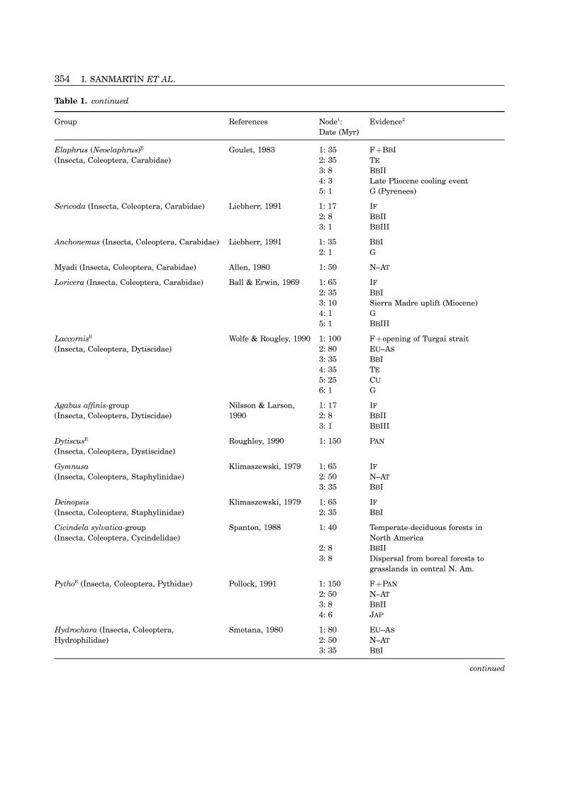
Table 1. Overview of the 57 Holarctic groups analysed in this study. For the 39 phylogenies that were dated in someanalyses, the age and evidence used for dating is given for each dated node (see Appendix for the position of the datednodes in the phylogenies)
Group References Node1: Evidence2
Date (Myr)
Xestia (Schoyenia) Lafontaine et al., 1983 1: 2 IF
(Insecta, Lepidoptera, Noctuidae) 2: 1 BBIII
Trichosilia Lafontaine & 1: 17 IF
(Insecta, Lepidoptera, Noctuidae) Kononenko, 1986 2: 8 BBII
SathonE Williams, 1988 1: 50 F+N-AT
(Insecta, Hymenoptera, Braconidae) 2: 25 CU
3: 8 BII4: 6 North and South America connected
Symmorphus debilitatus-groupE Cumming, 1989 1: 17 F+IF
(Insecta, Hymenoptra, Vespidae) 2: 8 BBII3: 6 JAP
IbaliidaeE Nordlander et al., 1996 1: 150 PAN
(Insecta, Hymenoptera) Ronquist, 1999 2: 8 BBII3: 6 JAP
4: 1 BBIII
LimnoporusE (Insecta, Hemiptera, Gerridae) Andersen & Spence, 1: 55 F1992 2: 35 BBIAndersen, 1993 3: 6 JAP
4: 1 BBIII
AquariusE (Insecta, Hemiptera, Gerridae) Andersen, 1990 1: 55 F
Nabicula (Limnonabis) Asquith & Lattin, 1990 1: 150 IF
(Insecta, Heteroptera, Nabidae) 2: 80 EU–AS
3: 50 N–AT
4: 25 CU
Nephrotoma dorsalis-groupE Tangelder, 1988 1: 35 F+TE
(Insecta, Diptera, Tipulidae) 2: 15 HIM
3: 10 Development of grasslands (GreatPlains)
4: 8 Development of boreal forests5: 6 JAP
6: 3.5 Opening of Bering strait7: 2 Spread of arctic conditions
PotamanthidaeE (Insecta, Ephemeroptera) Bae & McCafferty, 1: 150 F+PAN
1991 2: 35 TE
3: 35 Formation of the South China sea4: 8 Late Miocene cooling
BlethisaE (Insecta, Coleoptera, Carabidae) Goulet & Smetana, 1: 17 F+IF
1983 2: 8 BBII3: 1 BBIII
Elaphrus (Elaphroterus)E Goulet, 1983 1: 35 F+IF
(Insecta, Coleoptera, Carabidae) 2: 35 BBI3: 1 BBIII
continued
354 I. SANMARTIN ET AL.
Table 1. continued
Group References Node1: Evidence2
Date (Myr)
Elaphrus (Neoelaphrus)E Goulet, 1983 1: 35 F+BBI(Insecta, Coleoptera, Carabidae) 2: 35 TE
3: 8 BBII4: 3 Late Pliocene cooling event5: 1 G (Pyrenees)
Sericoda (Insecta, Coleoptera, Carabidae) Liebherr, 1991 1: 17 IF
2: 8 BBII3: 1 BBIII
Anchonemus (Insecta, Coleoptera, Carabidae) Liebherr, 1991 1: 35 BBI2: 1 G
Myadi (Insecta, Coleoptera, Carabidae) Allen, 1980 1: 50 N–AT
Loricera (Insecta, Coleoptera, Carabidae) Ball & Erwin, 1969 1: 65 IF
2: 35 BBI3: 10 Sierra Madre uplift (Miocene)4: 1 G5: 1 BBIII
LaccornisE Wolfe & Rougley, 1990 1: 100 F+opening of Turgai strait(Insecta, Coleoptera, Dytiscidae) 2: 80 EU–AS
3: 35 BBI4: 35 TE
5: 25 CU
6: 1 G
Agabus affinis-group Nilsson & Larson, 1: 17 IF
(Insecta, Coleoptera, Dytiscidae) 1990 2: 8 BBII3: 1 BBIII
DytiscusE Roughley, 1990 1: 150 PAN
(Insecta, Coleoptera, Dystiscidae)
Gymnusa Klimaszewski, 1979 1: 65 IF
(Insecta, Coleoptera, Staphylinidae) 2: 50 N–AT
3: 35 BBI
Deinopsis Klimaszewski, 1979 1: 65 IF
(Insecta, Coleoptera, Staphylinidae) 2: 35 BBI
Cicindela sylvatica-group Spanton, 1988 1: 40 Temperate-deciduous forests in(Insecta, Coleoptera, Cycindelidae) North America
2: 8 BBII3: 8 Dispersal from boreal forests to
grasslands in central N. Am.
PythoE (Insecta, Coleoptera, Pythidae) Pollock, 1991 1: 150 F+PAN
2: 50 N–AT
3: 8 BBII4: 6 JAP
Hydrochara (Insecta, Coleoptera, Smetana, 1980 1: 80 EU–AS
Hydrophilidae) 2: 50 N–AT
3: 35 BBI
continued

HOLARCTIC BIOGEOGRAPHY 355
Table 1. continued
Group References Node1: Evidence2
Date (Myr)
PlateumarisE Askevold, 1991 1: 150 F+PAN
(Insecta, Coleoptera, Chrysomelidae) 2: 80 MCS3: 25 CU
4: 1 G (Nearctic)
HypochilusE Catley, 1994 1: 150 F+PAN
(Arachnida, Araneae, Hypochilidae) 2: 25 CU
3: 1 G (Illinoisan)
PimoaE (Arachnida, Araneae, Pimoidae) Hormiga, 1994 1: 80 F+EU–AS
2: 35 BBI
CallilepisE Platnick, 1975, 1976 1: 80 F+PAN+EU–AS
(Arachnida, Araneae, Gnaphosidae) 2: 50 N–AT
3: 35 BBI4: 25 CU
EsoxE (Teleostei, Esocidae) Nelson, 1972 1: 65 F2: 50 N–AT
UmbridaeE (Teleostei) Wilson & Veilleux, 1: 65 F1982 2: 50 N–AT
3: 1 BBIII
CatostomidaeE (Teleostei) Smith, 1992 1: 65 F2: 50 F3: 22 F4: 8 F
OncorhynchusE Shedlock et al., 1992 1: 5 / 2: 4.5 / 3: MC
(Teleostei, Salmonidae) Domanico & Philips, 4.3. 4: 3.5 / 5:1995 2: 9 / 6: 2.6 / 7:
2.5
AlectorisE Randi, 1996 1: 6 / 2: 2.4 / 3: MC
(Aves, Galliformes, Phasianidae) 2.0 / 4: 1.0 / 5:1.2 / 6: 3
AnthusE Voelker, 1999a,b 1: 7 / 2: 5.6 / 3: MC
(Aves, Passeriformes, Motacillidae) 4.2 / 4: 2.7 / 5:1.3 / 6: 1.8 / 7:0.9 / 8: 4.7 / 9:2.3
Sorex longirostris-groupE George, 1988 1: 2 F(Mammalia, Soricidae) 2: 1.5 G (Wisconsinan)
3: 1 BBIII
UrsidaeE Talbot & Shields, 1996 1: 12.5 / 2: 7 / 3: MC
(Mammalia, Carnivora) Zhang & Ryder, 1994 6 / 4: 5 / 5: 1.5 /6: 5 / 7: 6.1
ChabaudgolvaniaE Adamson & 1: 35 F (fossil of host)+BBI(Nematoda, Ascaridida, Quimperiidae) Richardson, 1989
continued

356 I. SANMARTIN ET AL.
Table 1. continued
Group References Node1: Evidence2
Date (Myr)
Daphnia longispina-groupE Taylor et al., 1996 (cladograms 1 and MC+F(Crustacea, Cladocera) Lehman et al., 1995 2) ∗ 1: 100 / 2: 100 MC
3: 53 / 4: 6 / 5:1.8 / 6: 1.4 / 7: 1 /8: 3.5 / 9: 1 / 10:26.5 / 11: 30(cladogram 3) ∗1:1002: 53 / 3: 6 / 41.8 / 5: 1.4 / 6: 1 /7: 3.5 / 8: 1 / 9:26.5 / 10: 65 / 11:30
Heterotrissocladius (Insecta, Diptera, Saether, 1975Chrinomidae)Hydrobaenus (Insecta, Diptera, Saether, 1976Chironomidae)Mosillus (Insecta, Diptera, Ephydridae) Mathis et al., 1993Pachyneuridae (Insecta, Diptera) Wood, 1981Lotophila (Insecta, Diptera, Sphaeroceridae) Norrbom & Kim, 1984
Norrbom & Marshall, 1988Keroplatus (Insecta, Diptera, Keroplatidae) Matile, 1990Rocatelion (Insecta, Diptera, Keroplatidae) Matile, 1990Coelosia (Insecta, Diptera, Mycetophilidae) Soli, 1997Paraclemensia (Insecta, Lepidoptera, Nielsen, 1982Incurvariidae)Nitidotachinus (Insecta, Coleoptera, Campbell, 1993Staphylinidae)Lygus (Insecta, Heteroptera, Miridae) Schwartz & Foottit, 1998Atractotomus (Insecta, Heteroptera, Miridae) Stonedahl, 1990Oxyethira (Insecta, Trichoptera, Kelley, 1985Hydroptilidae)Flexamia (Insecta, Homoptera, Cicadellidae) Dietrich et al., 1997Taenionema (Insecta, Plecoptera, Stanger & Baumann, 1993Taeniopterygidae)Gasterosteiformes (Pisces, Teleostei) Paepke, 1983Larus (Aves, Ciconiiformes, Laridae) Chu, 1998Marmota (Mammalia, Rodentia, Sciuridae) Kruckenhauser et al., 1998
∗Three different solutions of the trichotomy (see Appendix).E Groups belonging to the externally dated set (only nodes dated with external evidence were considered in this analysis).1 Numbers refer to the numbered nodes in the cladogram of each group (see Appendix).2 Dating evidence: F=Fossil, G=Vicariance during Pleistocene glaciations, IF=Inferred from the age of a younger, datednode, MC=Molecular clock, PAN=Laurasia–Gondwana vicariance, TE=Vicariance due to the climatic cooling at the TerminalEocene event. Other codes (BBI, CU, MCS) are explained in Table 4. Only F, MC and PAN datings are considered based onexternal evidence (the externally dated set).

HOLARCTIC BIOGEOGRAPHY 357
Non-Holarcticevents
OthersSpiders
Mammals
Birds
Fishes
Insects
EP
WPEN
WN
Young
Recent
Medium
OldMolecularFossil
Holarcticevents
A B
C D
Figure 5. Pie charts summarizing various aspects of the data set analysed in this paper. (A) Taxonomic composition(number of groups). (B) Number of terminal taxa distributed in each Holarctic infraregion. (C) Type of evidence usedfor testing the basal divergence of each group (number of groups per category): fossil record (Fossil), molecular clock(Molecular), non-Holarctic biogeographic events (Non-Holarctic events), and Holarctic biogeographic events listed inTable 4 (Holarctic events). (D) Number of groups whose first divergence event is included within each time class.
wanted our results to be comparable with those of These terranes rifted from the margin of eastern Gond-wana during the Late Carboniferous–Early PermianEnghoff (1995). Thus, the Holarctic was divided into
four infraregions, each corresponding to a historically but were part of the Laurasian landmass by the LateTriassic–Early Jurassic (Yin, 1994). During the Earlypersistent landmass according to palaeogeographic re-
constructions (Cox, 1974): the eastern and western Tertiary, they were covered by the same boreotropicalflora as Japan and China, indicating that, at leastNearctic and the eastern and western Palaeoarctic.
The eastern Nearctic (EN) was defined as North Amer- during that period, connections existed between theeastern Palaeoarctic and Oriental regions (Wolfe, 1977;ica east of the former Mid-Continental Seaway; the
western Nearctic (WN) as North America west of the Tiffney, 1985a).The distribution of taxa was interpreted accordingMid-Continental Seaway; the western Palaeoarctic
(WP) as Europe, North Africa and Asia west of the to the original study. For example, if the author statedthat a taxon occurs mainly in WN and that EN recordsformer Turgai Sea; and the eastern Palaeoarctic (EP)
as non-tropical Asia east of the Turgai Sea. are sporadic, unreliable, or due to late dispersal, thetaxon was scored exclusively as WN.The Holarctic region and its infraregions were in-
terpreted in a wide sense. Thus, many Mexican dis- The western Palaeoarctic is the least representedinfraregion in the data set (n=158) (Fig. 5B). Thetributions were considered as western Nearctic
because Central America was connected to WN during western Nearctic is the most common infraregion (n=289), followed by the eastern Nearctic (n=263) andthe time of the Mid-Continental Seaway, and many
Mexican taxa show close relationships with western the eastern Palaeoarctic (n=248). This is significantlydifferent from expected if taxa were equally distributedNorth America via the Cordilleran Mountain System
(Liebherr, 1991). However, tropical Mexican dis- in the four infraregions (‘goodness of fit’ �2=40.6, df=3, P<0.01). Comparison with the geographic dis-tributions were considered as outside occurrences (NT
in Appendix). Similarly, taxa occurring in the northern tribution of species in groups whose Holarctic faunais well known suggests that, in our data set, the easternpart of the Oriental region (e.g. northern India
(Burma), South China, Indochina, northwest Thailand, Palaeoarctic is underrepresented and the Nearctic pos-sibly over-represented (Table 2).West Malaysia) were scored as eastern Palaeoarctic.

358 I. SANMARTIN ET AL.
and the area cladogram by extinction (possible vicar-ANALYSESiance events within the widespread terminal not coun-
Testing the hierarchical scenario ted); and the free option treats the widespread terminalAn event-based tree-fitting criterion, Maximum Vicar- as an unresolved higher taxon consisting of one lineageiance (MV) (Page, 1995; see also Ronquist, 1998a,b) was occurring in each area, and permits any combinationused to test for the existence of a general hierarchical of events and any resolution of the terminal polytomyvicariance pattern for the Holarctic. MV was used to in explaining the wide distribution.fit each of the 18 possible labelled histories for the four All possible dichotomous resolutions were consideredHolarctic infraregions (Fig. 6) in turn to all the 57 for polytomous cladograms. Each alternative di-cladograms in the data set using TreeFitter 1.0 (Ron- chotomous cladogram was weighted such that the sumquist, 2001). MV finds the maximum number of vicar- of the alternatives corresponded to the single clado-iance events that can be explained by a particular gram of a fully resolved group. Thus, if there werehierarchical scenario given the data set, disregarding three possible dichotomous cladograms, the resultsthe other events that must be postulated. The larger from each were weighted with 1/3.the number of vicariance events, the better the hier-archical scenario explains the observed data.
General Holarctic patternsTo test for significant fit between the best hier-archical scenario and the data set, we randomly per- Dispersal–vicariance analysis (DIVA; Ronquist, 1996,
1997), an event-based parsimony method, was used tomuted the terminal distributions in the original dataset 10 000 times and then calculated the fit between find general biogeographic patterns in the data set.
Unlike other methods, DIVA does not enforce hier-each random data set and the best hierarchical scen-ario using TreeFitter 1.0. The P value was estimated archical area relationships so it can be used to address
reticulate biogeographic scenarios. DIVA was first usedas the proportion of the random data sets fitting thebiogeographic scenario at least as well as the original to infer the biogeographic history of each individual
group. If several equally optimal reconstructions ex-data.Widespread taxa (taxa distributed in more than one isted, all alternatives were considered and each pos-
sibility down-weighted such that the sum of allarea) pose a problem for reconstructing hierarchicalpatterns because they introduce ambiguity in the data alternatives corresponded to a single unambiguous
reconstruction. DIVA reconstructions specify vicar-set (Morrone & Crisci, 1995). This problem has not yetbeen satisfactorily solved in the literature. Here, we iance events, dispersal events, diversification events
(speciation within a single unit area), and ancestraltreated widespread taxa using each of three novelevent-based options (Ronquist, in press). The recent distributions (allowing assessment of past species rich-
ness in different unit areas). The frequencies of theseoption assumes that the wide distribution is of recentorigin and explains it by dispersal; the ancient option inferred events and ancestral distributions were
summed over all 57 cladograms.considers the wide distribution to be of ancient originand explains any mismatch between the distribution We assessed the significance of the results in two
Table 2. Species richness in each Holarctic infraregion for some well-documented groups. Introduced species have notbeen counted, nor have species only occurring in areas formerly covered by the Mid-Continental Seaway or the TurgaiSea. The number of species per infraregion in our data set is also shown
Number of species
Taxon WN EN WP EP
Testudines1 (except Chelonidae and Dermochelyidae) 12 25 9 23Amphibia2 73 126 76 262Aves3 476 318 435 800Total 561 469 520 1085
(21%) (18%) (20%) (41%)Holarctic data set (this study) 289 263 158 248
(30%) (27%) (16%) (26%)
1 Iverson (1992).2 Frost (1985), Duellman (1993).3 Howard & Mooe (1991).

HOLARCTIC BIOGEOGRAPHY 359
Figure 6. The 18 possible hierarchical scenarios for the Holarctic region. There are 15 possible branching arrangementsof the four Holarctic infraregions. However, each of the three symmetrical branching arrangements produces twoposssible labelled histories if the sequence of the splitting events is taken into account (the first two and the fourbottom scernarios). This gives a total of 18 scenarios.
steps. First, we tested whether DIVA detected any Holarctic patterns over timeoverall patterns that were phylogenetically conserved In order to analyse the variation of biogeographicby comparing the observed total cost over all 57 cla- patterns over time, DIVA-inferred events were sorteddograms with the total cost over each of 100 data into time classes.sets for which the terminal distributions had beenrandomly shuffled. Second, we tested whether therelative frequency of particular biogeographic events, Events. The frequencies of most dispersal events were
too low to infer patterns of variation through time.relating to the hypotheses we wanted to test, differedfrom what would be expected by chance by a modified Instead, the variation in the frequency of two-area
distributions was used as an indicator of the ap-�2-test, in which the expected frequency and the ref-erence distribution were both calculated from 100 ran- pearance and disappearance of dispersal barriers.
When two isolated areas become connected, the cor-domly permuted data sets. For simplicity, thispermutation-based test statistic will be labelled �2 but responding two-area distributions should increase in
frequency. As long as the areas are connected, the two-it should not be confused with an ordinary �2-test usingthe standard �2 distribution to assess significance. area distributions should remain common. When a

360 I. SANMARTIN ET AL.
dispersal barrier separates the connected areas, we did originate during the Quaternary according to theauthor(s) of the original paper (e.g. Sorex longirostris-expect to see massive vicariance across the barrier and
concomitant decrease in the frequency of the two-area group). Non-Holarctic biogeographic events that wereuseful for dating included the split up of Pangaea (150distributions. We also recorded the variation in species
richness and diversification in each infraregion over Myr) and the formation of a land bridge betweenNorthern and Southern America (6 Myr) (Pielou, 1979).time.Twenty-seven of the phylogenies could be at leastpartially dated using these techniques (Fig. 5C).
Time classes. Age estimates (see below) suggest that In the fully dated set we used certain Holarcticthe biogeographic events documented by the clado- biogeographic events as additional temporal referencegrams span from the Late Mesozoic to the present. points. The idea was to increase temporal resolutionThis period was divided into four time classes (Table for patterns other than those used for dating and to3): old (before 70 Myr), medium (70–20 Myr), young allow dating of more phylogenies. Table 4 shows the(20–3 Myr), and recent (3–0 Myr). A finer division vicariance events that were used and the dates as-into more traditional geological periods (e.g. Eocene, signed to each of them. In the case of vicariance in-Oligocene, Miocene, etc.) was not feasible because the volving the Beringian land bridges, the habitatdated events were too few, particularly in the older specificity of each group was used to assign the eventtime periods. Time classes were delimited based on to the correct bridge (Table 4). Occasionally, the datedtwo criteria: (a) they must be wide enough to contain event was associated with a terminal species, in whicha sufficient number of cladogenetic events in our phylo- case the date was assigned to the terminal node itself.genies; and (b) each time class should preferably con- To reduce investigator bias, the events listed in Tabletain or be delimited by only one of the postulated 4 were only used for dating if they were explicitlyHolarctic dispersal-vicariance events of interest. The mentioned in the original study. Our dating, however,latter was not always possible to achieve. For instance, does not necessarily coincide with that of the authors,the medium time class included both the trans-Atlantic since the biogeographic-geologic events used for datingbridge (50 Myr) and the first Beringian Bridge (35 took place during a time interval. For example, vicar-Myr). To separate trans-Atlantic and trans-Beringian iance across the first Beringian bridge was dated asdispersal routes, we used another division into four 35 Myr, although dispersal of temperate groups wastime classes, in which the medium time class was possible after that date. Patterns that could not bedivided into two subclasses, 70–45 and 45–20 Myr, dated unambiguously, such as the disjunctions EN–EPwhile the young and recent time classes were pooled. and WN–WP, were not used for dating even if theyThe time boundary of 45 Myr was chosen to assure were dated in the original study.that, in the younger time class, the dispersal route If the age of one or more internal nodes but not thebetween North America and Eurasia had switched basal node could be fixed using biogeographic eventsdefinitely to Beringia from having been predominantly listed in Table 4, the basal node was assigned a dateNorth Atlantic. This hypothesized event, when the consistent with the age of the internal node(s). Thus,cross-Atlantic Thulean route broke up and Beringia the basal node was dated to 150 Myr in groups showingbecame warmer, has been dated to approximately 50 an internal Euramerica–Asiamerica vicariance (EU-Myr (Pielou, 1979). AS), to 65 Myr for groups with internal trans-Atlantic
(N-AT) or first trans-Beringian vicariance (BBI); to 17Myr for groups with internal second trans-BeringianDating. We used two different methods of dating,vicariance (BBII); and to 2 Myr for groups with internalresulting in two different dated subsets of the data:third trans-Beringian vicariance (BBIII). Thirty-ninethe externally and fully dated sets. Table 1 indicatesgroups could be at least partially dated using externalfor each cladogram the dated nodes and the evidence(molecular, fossil, or non-Holarctic events) or Holarcticused for dating them.reference points (Fig. 5C). The remaining 18 groupsIn the externally dated set, we used fossil evidence,could not be dated because of insufficient informationmolecular clock estimates or non-Holarctic bio-in the original study. The age (root node age) of allgeographic events for dating (Fig. 5C; Table 1). Mo-dated phylogenies is summarized in Figure 5D.lecular clock dates were taken from the original papers.
All clocks were calibrated with the fossil record of thegroup in question, except for the genus Anthus (Voelker, Branching clock. For both the fully and externally
dated sets, after the dates of one or more internal1999a). For fossil evidence, the oldest known fossil ofthe group was used to date the root node in the phylo- nodes had been fixed, a ‘branching clock’ was used to
determine the age of the remaining nodes. First, anygeny. Occasionally, some internal nodes were alsodated using fossil evidence (e.g., Catostomidae). Plei- dated interior nodes were connected to each other,
forming a backbone of dated nodes. This was done bystocene fossils were only used if the group actually

HOLARCTIC BIOGEOGRAPHY 361
Table 3. The four time classes used in this study. For each time class, the geological period covered by the time-class,the Holarctic biogeographic events that took place during that period (codes correspond to those in Table 4 and Fig.10), and the main characteristics of the groups that originated during that period, are given
Time class Time period Geological period Biogeographic events Groups originating in thisperiod
Old >70 Myr Late Mesozoic (before Euramerica–Asiamerica (EU–AS) Warm–temperate groupsLate Cretaceous) Groups with Southern
Hemisphere sister groups
Medium 70–20 Myr Early–Mid Tertiary Trans-Atlantic (N–AT) Warm–temperate groupsTrans-Beringian (BBI) associated with the
boreotropical–mixedmesophytic forest
Young 20–3 Myr Late Tertiary Trans-Beringian (BBII) Boreal groups associated withtaiga–coniferous forests
Recent 3–0 Myr Quaternary Trans-Beringian (BBIII) Arctic groups associated withtundra vegetation
Table 4. Holarctic dispersal–vicariance events used for dating ancestral nodes in the phylogeny of the groups studied(the fully dated set). For each biogeographic event, the geologic event that caused the vicariance, the habitat specificityof the groups affected by the event, and the date assigned to it, are given
Biogeographic event Code (date) Geologic event (habitat specificity)
Euramerica–Asiamerica EU–AS (80 (Myr) Separation of the palaeocontinents(WN+EP)–(EN+WP) Euramerica–Asiamerica
Trans-Atlantic (EN–WP) N–AT (50 Myr) Closing of the Thulean North Atlantic bridge1
(Warm–temperate groups)
Beringian bridge I BBI (35 Myr) Terminal Eocene event(WN–EP) (Warm–temperate groups)
Beringian bridge II BBII (8 Myr) Late Miocene–Pliocene cooling2
(WN–EP) (Boreal–coniferous groups)
Beringian bridge III BBIII (1 Myr) Arctic climates dominant (Arctic–tundra groups)(WN–EP)
Nearctic (WN–EN) (1) MCS (80 Myr) (1) Opening of Mid-Continental Seaway(2) CU (25 Myr) (2) Uplift of Cordilleran Mountain System4
Palaeoarctic (WP–EP) PAL (30 Myr) Closing of Turgai Strait
Other minor events:Himalaya–Central Asia (1) HIM (15 Myr) (1) Himalayan orogenyJapan–Continental Asia (2) JAP (6 Myr) (2) Opening of Japanese Sea
1 Subsequent North Atlantic land bridges (Late Eocene–Miocene) were presumably restricted to cold-adapted groups and farless important for cross-Atlantic faunal exchange (McKenna, 1983).2 Although the opening of the Bering Strait took place at 3.5 Myr, most authors explain trans-Beringian vicariance of borealgroups as a result of increasing climate cooling during the Later Miocene–Pliocene.4 Mountain folding continued through the Miocene but most authors indicate the Late Oligocene as the age of the mainorogenic phase (Tiffney, 1985b). In some cases, the second Nearctic vicariance was dated 35 Myr if the author explained thisvicariance as a result of the Late Eocene cooling event.

362 I. SANMARTIN ET AL.
Figure 7. Schematic illustration of the branching clock method of estimating node dates. First, the longest sequenceof speciation events linking the dated root (r) to a terminal is identified (thick line). Then the branches in this sequenceare assigned equal time duration (50 Myr/5=10 Myr). Finally, the remaining undated nodes (labelled a and b) areassigned one of the dates in this sequence. (A). In delayed speciation, the undated nodes are assigned the youngestpossible date. (B) In accelerated speciation, the undated nodes are assigned the oldest possible date.
first connecting the nodes separated by the fewest was determined based on the distributions of the ter-minals. If these distributions were permuted, the dat-intermediate nodes. These intermediate nodes were
then dated assuming equal branch lengths in the path ing of the nodes would be nonsensical.between the dated nodes. Then, the next dated nodeclosest to this backbone was connected and the inter-
RESULTSmediate nodes dated, until all dated nodes had beenconnected. Then, each tip of the dated backbone, which TESTING THE HIERARCHICAL SCENARIOoften consisted of only the root node (Fig. 7; node r),
Figure 8 shows the cost of fitting each of the 18 possiblewas connected to one of the terminal nodes from whichhierarchical scenarios to the 57 phylogenies in ourit was separated by the largest number of speciationdata set. Regardless of the event-based option used toevents (Fig. 7; bold line). Each branch in that sequencetreat widespread taxa (free, ancient or recent), thewas assumed to have the same time duration. Finally,hierarchical scenarios 1 and 2 (Fig. 6) showed the bestall remaining undated nodes (Fig. 7; node a and b)fit (the maximum number of vicariance events). Thesewere assigned one of the dates of the nodes in thescenarios correspond to the same area cladogram ((WN,closest dated clade by using one of two differentEN), (WP, EP)), depicting a basal separation of Northmethods. In delayed speciation, each node was assignedAmerica and Eurasia followed by eastern–westernthe youngest possible date (Fig. 7A); in acceleratedvicariance within each continent. They only differ inspeciation, the oldest possible date was used insteadthat scenario 1 assumes the eastern–western division(Fig. 7B).to be older in the Palaeoarctic than in the Nearctic,whereas the reverse is true for scenario 2 (Fig. 6).
The difference in number of vicariance events be-Significance tests. To identify significant variation inthe frequency of biogeographic patterns over time, tween the best and the worst scenarios is quite small
for the recent option but distinctly larger for the ancientas evidenced by external dating, we compared theobserved frequencies in each time class with the ex- option (Fig. 8). For the free option, the relative dif-
ference is small but the absolute difference is similarpected frequencies from 100 random data sets in whichterminal distributions were randomly permuted. The to the ancient option. Recall that the ancient option
forces wide terminal distributions to be interpretedpermutation test could not be used with the fully datedset, since the age of some internal nodes in this set as supporting area relationships, whereas the recent

HOLARCTIC BIOGEOGRAPHY 363
018
180C
1 2 3 4 5 6 7 8 9 10 11 12 13 14 15 16 17
150120906030
018
80
B
1 2 3 4 5 6 7 8 9 10 11 12 13 14 15 16 17
60
40
20
018
300A
1 2 3 4 5 6 7 8 9 10 11 12 13 14 15 16 17
25020015010050
Figure 8. Bar diagrams showing the results of fitting each of the 18 Holarctic hierarchical scenarios (Fig. 6) to theentire data set of 57 Holarctic animal groups: (A) Free (P>0.99); (B) Ancient (P>0.99); (C) Recent (P>0.99). TheMaximum vicariance (Page, 1995; Ronquist, 1998a,b) criterion was used and the exact cost of each scenario wascalculated using TreeFitter 1.0 (Ronquist, 2001). Maximum vicariance maximizes the number of vicariance events inthe data that can be explained by the given scenario. Widespread taxa were treated using one of three event-basedoptions: free, ancient or recent (see text). The statistical significance of the fit of the best scenario to the data wastested by comparison with the expected number of vicariance events in 10 000 data sets in which the distributions hadbeen randomly permuted in each group. For all options of treating widespread taxa, the fit was found to be non-significant (P>0.9999). This extraordinarily high P value is caused by strong distribution duplication patterns (seetext).
option never builds area relationships on widespread was no hierarchical vicariance pattern that could ad-equately describe the data.taxa. Thus, the small difference under the recent option
indicates that the support for the best scenarios under We also analysed Enghoff’s (1995) data sets: thegenus clades (groups at the genus level or below) andthe other options mainly comes from the prevalence of
wide continental distributions (WN+EN or WP+EP) the family clades (groups at the family level or above).For the genus clades, the best hierarchical scenariosamong terminals, whereas internal nodes essentially
group distributions randomly. were numbers 1 and 2 (Fig. 6) (corresponding to RAC13 in Enghoff, 1995) but the fit was not statisticallyPermutations of the distributions showed that, re-
gardless of the option used for widespread taxa, the significant, regardless of option used for widespreadtaxa (P=0.95 for all options). For the family clades,best hierarchical scenarios did not fit the data set
significantly better than expected by chance. Actually, the best hierarchical scenarios were again 1 and 2for the free and ancient options but the fit was notall 10 000 random data sets had more vicariance events
than the original data, a highly significant result run- statistically significant (P=0.80 for the free option andP=0.65 for the ancient option). For the recent option,ning in the opposite direction of the expected outcome
(P>0.9999). Such apparently anomalous results are however, the best hierarchical scenario was number17 (Fig. 6), which showed a statistically significant fitexpected in maximum vicariance analysis when local
diversification (duplication) is common (Ronquist, in to the data (P=0.01). Scenario 17 has an initial splitbetween Euramerica and Asiamerica, followed bypress). In any case, these results indicated that there

364 I. SANMARTIN ET AL.
further division within these palaeocontinents, the EN–EP and WN–WP disjunctionsfirst being within Euramerica (Fig. 6). There is no significant difference between the fre-
quency of the eastern North America–eastern Pal-aeoarctic dispersals (EN↔EP) and the western North
GENERAL HOLARCTIC PATTERNS America–western Palaeoarctic dispersals (WN↔WP)Overall, DIVA analysis indicated less dispersal for the (�2=0.000002, P>0.99). Dispersal from western Pal-original data set than for any of the 100 permuted aeoarctic to western North America (WP→WN) is sig-data sets. Thus, the observed number of dispersal nificantly more frequent than in the other directionevents is significantly smaller than expected by chance (WN→WP) (�2=3.692, P<0.01), whereas there is no(P<0.01), which means that the observed distributions directional dispersal asymmetry for the EN–EP dis-are strongly phylogenetically conserved. junction.
Table 5 and Figure 9 show comparisons of the ob-served and expected frequencies of different types of
Diversity differencesdispersal events. Several general patterns were found.The distribution of species richness among infra-regions, summing over all ancestral nodes but dis-regarding terminal species, is significantly differentLarge scale patternsfrom the distribution expected if species were dis-Continental dispersals (WN↔EN and WP↔EP) aretributed randomly with respect to infraregion (�2=significantly more frequent than palaeocontinental38.891, df=3, P<0.01). The western Palaeoarctic (WP)(WN↔EP and EN↔WP) and disjunct (EN↔EP andhas the smallest diversity (153 ancestral species), fol-WN↔WP) dispersals (�2=6.434, P<0.01). Palaeo-lowed by EP (244), EN (264) and WN (273) (cf. Fig.continental dispersals, in turn, are significantly more5B, giving the species richness for extant species). Thefrequent than disjunct dispersals (�2=1.965, P<0.01).amount of diversification (the number of speciationevents within each infraregion) is similarly distributed(WP=43, EP=116, EN=135, WN=138; �2=54.796,Continental patternsP<0.01). These differences, however, are the result ofThe absolute number of dispersals within the Nearcticthe unequal representation of the four infraregionsregion (WN↔EN) is larger than the number of dis-among terminal species. If the observed values arepersals within the Palaeoarctic region (WP↔EP). How-compared with the expected values obtained in theever, when compared with expected frequencies, therandom data sets, i.e. correcting for the regional biasopposite pattern is found: Palaeoarctic faunal exchangein extant faunal richness, differences are not sig-is significantly more frequent than expected by chancenificant (P=0.78 for species richness, and P=0.87 for(�2=3.389, P<0.01). Within each continent, there isdiversification). Thus, there are no phylogeneticallysignificant directional asymmetry. Dispersal fromdetermined differences in overall species richness orwestern North America to eastern North Americaoverall diversification rate among infraregions in our(WN→EN) is significantly more frequent than in thedata set.other direction (EN→WN): (�2=2.656, P=0.03). In
the Palaeoarctic, westward dispersals (EP→WP) aresignificantly more frequent than eastward dispersals HOLARCTIC PATTERNS OVER TIME(WP→EP): (�2=2.542, P=0.01).
Dating accuracy
With external dating, the branching clock was used toTrans-Beringian and trans-Atlantic exchange estimate the age of many internal nodes. Some of these
nodes could also be dated using Holarctic biogeographicIn absolute numbers, trans-Beringian dispersal be-tween the eastern Palaeoarctic and western North events (Table 4). This provided a useful test of the
branching clock (Fig. 10; results shown for delayedAmerica (WN↔EP) is more frequent than trans-At-lantic dispersal between eastern North America and speciation). The comparison reveals that the branching
clock does well, at least for the older biogeographicthe western Palaeoarctic (EN↔WP). However, the dif-ference is not significant (�2=0.0062; P=0.87). West- events. In most cases, it appears to sort events correctly
into one of the four broadly defined time classes weern North America (WN→EP) is more frequently thesource area of trans-Beringian dispersal than the east- used. The most serious problem is with the younger
events, which are consistently dated as being olderern Palaeoarctic (EP→WN), contrary to expectations,but the difference is not significant (�2=0.597, P= than they are by the branching clock (Fig. 10). This
bias is expected since the branching clock distributes0.32). There is no significant directional asymmetry inthe trans-Atlantic faunal exchange (EN↔WP) (�2= nodes equally over time whereas, if speciation rates
are roughly clock-like, extinctions will make sure that1.221, P=0.23).
HOLARCTIC BIOGEOGRAPHY 365
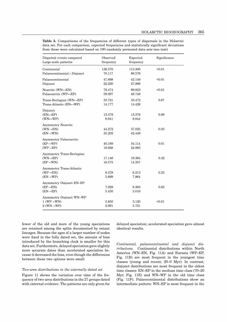
Table 5. Comparisons of the frequencies of different types of dispersals in the Holarcticdata set. For each comparison, expected frequencies and statistically significant deviationsfrom these were calculated based on 100 randomly permuted data sets (see text)
Dispersal events compared Observed Expected SignificanceLarge-scale patterns frequency frequency
Continental 138.570 113.300 <0.01Palaeocontinental+Disjunct 70.117 86.576
Palaeocontinental 47.898 42.149 <0.01Disjunct 22.220 27.968
Nearctic (WN↔EN) 79.474 89.823 <0.01Palaeoarctic (WP↔EP) 59.097 48.748
Trans-Beringian (WN↔EP) 33.721 33.472 0.87Trans-Atlantic (EN↔WP) 14.177 14.426
Disjunct(EN↔EP) 13.379 13.376 0.99(WN↔WP) 8.841 8.844
Asymmetry Nearctic(WN→EN) 44.272 37.025 0.03(EN→WN) 35.202 42.449
Asymmetry Palaeoarctic(EP→WP) 40.169 34.114 0.01(WP→EP) 18.928 24.983
Asymmetry Trans-Beringian(WN→EP) 17.146 19.364 0.32(EP→WN) 16.575 14.357
Asymmetry Trans-Atlantic(WP→EN) 8.278 6.213 0.23(EN→WP) 5.899 7.964
Asymmetry Disjunct EN–EP(EP→EN) 7.929 8.363 0.83(EN→EP) 5.450 5.016
Asymmetry Disjunct WN–WP1 (WP→WN) 5.850 3.120 <0.012 (WN→WP) 2.991 5.721
fewer of the old and more of the young speciations delayed speciation; accelerated speciation gave almostare retained among the splits documented by extant identical results.lineages. Because the ages of a larger number of nodeswere fixed in the fully dated set, the amount of biasintroduced by the branching clock is smaller for this
Continental, palaeocontinental and disjunct dis-data set. Furthermore, delayed speciation gave slightlytributions. Continental distributions within Northmore accurate dates than accelerated speciation be-America (WN–EN, Fig. 11A) and Eurasia (WP–EP,cause it decreased the bias, even though the differencesFig. 11B) are most frequent in the youngest timebetween these two options were small.classes (young and recent; 20–0 Myr). In contrast,disjunct distributions are most frequent in the oldest
Two-area distributions in the externally dated set time classes: EN–EP in the medium time class (70–20Myr; Fig. 11E) and WN–WP in the old time classFigure 11 shows the variation over time of the fre-(Fig. 11F). Palaeocontinental distributions show anquency of two-area distributions in the 27 groups dated
with external evidence. The patterns are only given for intermediate pattern: WN–EP is most frequent in the

366 I. SANMARTIN ET AL.
Figure 9. Diagrammatic, polar views of the Holarctic region, showing the frequency of dispersal between differentinfraregions in the data set. The thickness of the arrows is proportional to the frequency of the dispersal in question.Abbreviations: WN – western Nearctic, EN – eastern Nearctic, WP – western Palaoearctic, EP – eastern Palaeoarctic.
recent time class (Fig. 11C), whereas EN–WP is mostfrequent in the medium class (Fig. 11D).
Continental distributions. The frequency of Nearcticdistributions (WN–EN) shows a decrease in themedium time class, followed by a rapid increase in theyoung and recent time classes (Fig. 11A). This patterndiffers significantly from that expected by chance(P<0.01). The frequency of Palaeoarctic distributions(WP–EP) is low in the old and medium time classes(>20 Myr) but increases rapidly in the young timeclass (20–3 Myr; Late Tertiary), followed by a slightdecrease in the recent time class (3–0 Myr; Fig. 11B).However, these differences were not significant (P=0.53).
Trans-Beringian and trans-Atlantic distributions. Thefrequency of trans-Beringian distributions (WN–EP)decreases over time with the lowest value being in theyoung time class (20–3 Myr), followed by a strongincrease in the recent time class (3–0 Myr; Fig. 11C).
0EU–AS
108
Tim
e (M
yr)
N–AT JAPCORDBBIIIBBIIBBI
102
8121824303642485460
7278849096
66
MaxMinMean + SDMean – SDMean
Differences among frequencies were significantly con-strained by phylogeny (P<0.01). The frequency of trans-Figure 10. Plot showing the accuracy of the branchingAtlantic distributions (EN–WP) shows a distinct peakclock assessed by the presumed dates of some Holarctic
biogeographic events (Table 4). The box-whisker plots in the medium time class and decrease strikingly inshow the estimated age of certain nodes (mean, standard the young and recent time classes (Fig. 11D). Thisdeviation and minimum and maximum values) using the pattern was close to being statistically significant (P=branching clock calibrated with external evidence (from 0.11).the fossil record, non-Holarctic biogeographic events, ormolecular evidence). The arrows indicate the presumed
EN–EP and WN–WP disjunct distributions. The fre-age of the same nodes according to Holarctic biogeographicquency of the disjunct distribution eastern Northevents (Table 4). The number of observations are asAmerica–eastern Palaeoarctic (EN–EP) increases rap-follows: Trans-Atlantic (N–AT, n=6), Beringian Bridge Iidly in the medium time class (70–20 Myr) to decrease(BBI, n=21), Beringian Bridge II (BBII, n=17), Beringianmarkedly in the young and recent time classes (20–0Bridge III (BBIII, n=15), Cordilleran orogeny (CORD,Myr; Fig. 11E). Again, differences among frequenciesn=8), Japanese sea (JAP, n=9), Euramerica–Asiamerica
vicariance (EU–AS, n=5). were close to being statistically significant (P=0.10).

HOLARCTIC BIOGEOGRAPHY 367
Time class (Myr)
–0.05
0.40
0.25
0.10
<3EN–WP
>70 <20<70
D P = 0.11
<3EN–EP
>70 <20<70
E P = 0.10
<3WN–WP
>70 <20<70
F P < 0.01
–0.05
0.40
Per
cen
tage
0.25
0.10
<3WN–EN
>70 <20<70
A P < 0.01
<3WP–EP
>70 <20<70
B P = 0.53
<3WN–EP
>70 <20<70
C P < 0.01
Figure 11. Frequency of the six possible two-infraregion distributions plotted against time for the externally datedset of 27 Holarctic groups. Because some time classes cover a longer time span than others, the frequency of each two-infraregion distribution is given as a percentage of the total number of two-infraregion distributions in each time class.Abbreviations: WN – western Nearctic, EN – eastern Nearctic, WP – western Palaeoarctic, EP – eastern Palaeoarctic.The P values are based on permutation tests.
In contrast, the frequency of the disjunct distribution suggesting a significant frequency change between thewestern North America–western Palaeoarctic (WN– medium and young time classes (Fig. 12B). Finally,WP) shows a constant decrease over time, with the the lowest frequency of trans-Beringian distributionspeak frequency in the old time class, before the Late shifts from the young (20–3 Myr; Fig. 11C) to theCretaceous (>70 Myr; Fig. 11F). This pattern is highly medium time class (70–20 Myr; Fig. 12C).significant (P<0.01).
The eastern North America–Asia disjunctionTwo-area distributions in the fully dated setThe age of this disjunction was examined in moreFigure 12 shows the frequency of two-area dis-detail by dividing the medium time class into twotributions over time for the 39 groups in the fully datedsubclasses (70–45 and 45–20 Myr), while pooling theset using delayed speciation (accelerated speciationyoung and recent time classes (Fig. 13). The frequencygave almost identical results). The observed bi-of the eastern North America–eastern Palaeoarcticogeographic patterns are similar to those found in the(EN–EP) distributions (Fig. 13C, D) and of trans-smaller externally dated set of phylogenies, with someAtlantic (EN–WP) distributions (Fig. 13E, F) showedexceptions. For WN–EN, the distributions are on av-a similar pattern of variation, with a sharp peak inerage dated older, such that the distinct increase inthe Early Tertiary time class (70–45 Myr). In contrast,the frequency of these distributions in the two youngestthe frequency of trans-Beringian (WN–EP) dis-time classes becomes more gradual (Fig. 12A). Thistributions dipped in the Early Tertiary, followed by anpresumably occurs because the Holarctic events usedincrease during the later time classes (Fig. 13A, B).for dating (Table 4) push these distributions back inThe peak of the EN–EP distributions was sharper intime. For the Palaeoarctic distributions (WP–EP), onthe externally dated set than in the fully dated set, inthe other hand, the increase in the youngest time
classes becomes more prominent in the fully dated set, which some (but less than 50%) of the EN–WP and
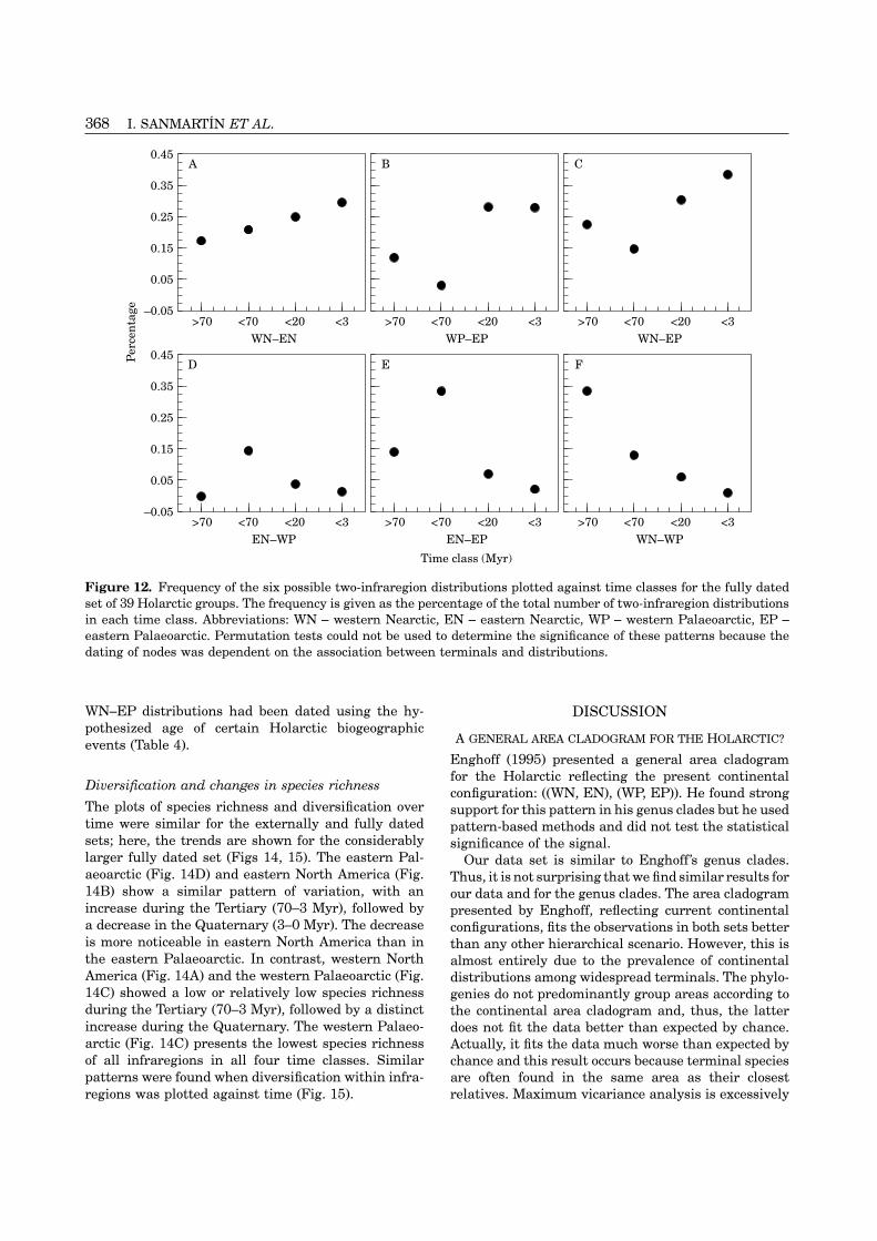
368 I. SANMARTIN ET AL.
Time class (Myr)
–0.05
0.45
0.25
0.05
<3EN–WP
>70 <20<70
D
<3EN–EP
>70 <20<70
E
<3WN–WP
>70 <20<70
F
0.45
Per
cen
tage
0.25
0.15
<3WN–EN
>70 <20<70
A
<3WP–EP
>70 <20<70
B
<3WN–EP
>70 <20<70
C
0.35
0.15
–0.05
0.05
0.35
Figure 12. Frequency of the six possible two-infraregion distributions plotted against time classes for the fully datedset of 39 Holarctic groups. The frequency is given as the percentage of the total number of two-infraregion distributionsin each time class. Abbreviations: WN – western Nearctic, EN – eastern Nearctic, WP – western Palaeoarctic, EP –eastern Palaeoarctic. Permutation tests could not be used to determine the significance of these patterns because thedating of nodes was dependent on the association between terminals and distributions.
WN–EP distributions had been dated using the hy- DISCUSSIONpothesized age of certain Holarctic biogeographic
A GENERAL AREA CLADOGRAM FOR THE HOLARCTIC?events (Table 4).Enghoff (1995) presented a general area cladogramfor the Holarctic reflecting the present continental
Diversification and changes in species richness configuration: ((WN, EN), (WP, EP)). He found strongThe plots of species richness and diversification over support for this pattern in his genus clades but he usedtime were similar for the externally and fully dated pattern-based methods and did not test the statisticalsets; here, the trends are shown for the considerably significance of the signal.larger fully dated set (Figs 14, 15). The eastern Pal- Our data set is similar to Enghoff’s genus clades.aeoarctic (Fig. 14D) and eastern North America (Fig. Thus, it is not surprising that we find similar results for14B) show a similar pattern of variation, with an our data and for the genus clades. The area cladogramincrease during the Tertiary (70–3 Myr), followed by presented by Enghoff, reflecting current continentala decrease in the Quaternary (3–0 Myr). The decrease configurations, fits the observations in both sets betteris more noticeable in eastern North America than in than any other hierarchical scenario. However, this isthe eastern Palaeoarctic. In contrast, western North almost entirely due to the prevalence of continentalAmerica (Fig. 14A) and the western Palaeoarctic (Fig. distributions among widespread terminals. The phylo-14C) showed a low or relatively low species richness genies do not predominantly group areas according toduring the Tertiary (70–3 Myr), followed by a distinct the continental area cladogram and, thus, the latterincrease during the Quaternary. The western Palaeo- does not fit the data better than expected by chance.arctic (Fig. 14C) presents the lowest species richness Actually, it fits the data much worse than expected byof all infraregions in all four time classes. Similar chance and this result occurs because terminal speciespatterns were found when diversification within infra- are often found in the same area as their closest
relatives. Maximum vicariance analysis is excessivelyregions was plotted against time (Fig. 15).

HOLARCTIC BIOGEOGRAPHY 369
D
Time class (Myr)
–0.1<20
0.4
EN–WP
Per
cen
tage
>70
0.3
0.2
0.1
0.0
<45<70
E
–0.05<20
0.55
EN–WP
>70
0.35
0.25
0.15
0.05
<45<70
F
–0.1<20
0.7
EN–EP
Per
cen
tage
>70
0.5
0.3
0.1
0.0
<45<70
C
–0.05<20
0.35
EN–EP
>70
0.25
0.15
0.05
<45<70
–0.1<20
0.4
WN–EP
Per
cen
tage
>70
0.3
0.2
0.1
0.0
<45<70
A
–0.05<20
0.35
WN–EP
>70
0.25
0.15
0.05
<45<70
B
0.45
0.6
0.4
0.2
Figure 13. Frequency of trans-Beringian (WN–EP), trans-Atlantic (EN–WP) and disjunct distributions (EN–EP)plotted against time for the externally dated set (27 groups) (A, C, E) and for the fully dated set (39 groups) (B, D, F).To increase resolution in the Early Tertiary, a different division into time classes was used. Note that some of thetrans-Beringian and trans-Atlantic events were dated according to the presumed age of the corresponding biogeographicevent in the fully dated set (B, F). However, the disjunct distributions (D) were not dated.
sensitive to such distribution duplication patterns a different hierarchical scenario is favoured, and thesupport for this scenario is significantly larger than(Ronquist, in press). When they are common, randomly
permuted data sets tend to have more vicariance events expected by chance. Recall that the recent option dis-regards any evidence for area relationships providedthan the observed data.
For the family clades, which presumably document by widespread terminals and only groups areas basedon older clades. Thus, the chance of detecting phylo-older biogeographic events, Enghoff (1995) did not
find a clearly dominant pattern using pattern-based genetically determined biogeographic patterns isbetter with the recent option than with the free andmethods. Under the free and ancient options of treating
widespread taxa, we find that the family clades behave ancient options.The scenario supported by the family clades underas the genus clades. However, under the recent option,

370 I. SANMARTIN ET AL.
Per
cen
tage
Time class (Myr)
0.08
0.44
0.20
WP
0.38
0.14
<3>70 <20<70
C
<3>70 <20<70
D
EP
WN
<3>70 <20<70
A
<3>70 <20<70
B
EN
0.260.32
0.08
0.44
0.20
0.38
0.14
0.260.32
Figure 14. Species richness per infraregion plotted against time for the fully dated set (39 groups) (the externallydated set showed similar trends). Species richness is measured as the number of nodes (ancestral species) occurringin each infraregion. To correct for the unequal duration of time classes, the species richness per region is given as thepercentage of the total species richness in each time class.
Per
cen
tage
Time class (Myr)
0.0
0.5
0.2
WP
0.4
0.1
<3>70 <20<70
C
<3>70 <20<70
D
EP
0.0
0.5
0.2
WN
0.4
0.1
<3>70 <20<70
A
<3>70 <20<70
B
EN
0.3
0.3
Figure 15. Diversification per infraregion plotted against time in the fully dated set (39 groups) (the externally datedset showed similar trends). Diversification is measured as the number of speciation events occurring exclusively withineach infraregion (i.e. among-region vicariance events are not considered). Diversification per region is given as thepercentage of the total number of diversification events in each time class.
the recent option is number 17 (Fig. 6). This scenario option in event-based analysis. However, because itwas not clearly dominant, he did not consider this ahas an initial division between the palaeocontinents
Euramerica and Asiamerica, followed by vicariance general Holarctic biogeographic pattern. Our analysisindicates that this is the only robust hierarchical pat-first within Euramerica and then within Asiamerica.
Interestingly, Enghoff (1995) found the same pattern tern in Enghoff’s (1995) data sets. Interestingly, thisMV result agrees well with the variation of two-area(his RAC 15) to be the most frequent for his family
clades when he treated widespread taxa using as- distributions over time in that it clearly dates theEuramerican (EN–WP) vicariance as being older thansumption 2, a pattern-based option similar to the free

HOLARCTIC BIOGEOGRAPHY 371
the Asiamerican (WN–EP) vicariance (compare scen- CONTINENTAL PATTERNSario 17 in Fig. 6 with Figs 11–13). Enghoff (1995) found that dispersals within North
In conclusion, although old Holarctic biogeographic America (WN↔EN) were more frequent in his dataevents documented by higher phylogenies appear to set than dispersals within the Palaeoarctic regionfit a Euramerican-Asiamerican pattern, it is clear that (WP↔EP). He did not test whether this difference wasno general area cladogram can adequately describe significant but he nevertheless attributed it to theHolarctic area relationships as evidenced by our data difference in duration of the epicontinental seaways,or the data of Enghoff’s genus clades. which were presumably important dispersal barriers
for the terrestrial and limnic fauna. The Nearctic wasdivided by the Mid-Continental Seaway for only 30
LARGE-SCALE HOLARCTIC PATTERNS Myr, from 100 to 70 Myr, while the Turgai StraitEnghoff (1995) found that continental dispersals divided the Palaeoarctic much longer, from 180 to 30(within the present continents) were significantly more Myr. However, the dominance of American dispersalsfrequent than palaeocontinental dispersals (between is probably entirely due to the overrepresentation ofareas once connected in the former continents American taxa in Enghoff’s data set. Using per-Asiamerica and Euramerica), and these in turn were mutation tests we find that, considering the numbermore frequent than disjunct dispersals (between infra- of lineages that could have dispersed, faunal exchangeregions never connected) in his data set of 73 Holarctic has actually been significantly more extensive in thegroups. This result was based on a test of deviation Palaeoarctic than in the Nearctic. This does not meanfrom equal probabilities of all dispersals. However, the that the Turgai Strait was not an effective barrier:Holarctic infraregions are not equally well represented the dated phylogenies show that almost all of thein his data set, nor are they in ours (Fig. 5B), and Palaeoarctic exchange occurred after the closing of thehence dispersal frequencies should be expected to differ Turgai Strait in the Oligocene, 30 Myr (Figs 11, 12).considerably even if they were assigned randomly to However, it does imply that faunal exchange has beencategories. Our test based on random permutation less extensive between the Nearctic infraregions afterof terminal distributions takes the unequal species the disappearance of the Mid-Continental Seaway thandiversity of different infraregions into account. Never- one might have expected.theless, Enghoff’s result holds: continental dispersals The variation in the frequency of Palaeoarctic dis-are more frequent than palaeocontinental dispersals, tributions over time (Figs 11, 12) fits palaeogeographicwhich are more common than disjunct dispersals. reconstructions well. During the time it was open, the
This pattern is undoubtedly an effect of time and past Turgai Strait apparently provided an effective barriercontinental connections (Enghoff, 1995). According to dispersal between the eastern and western Pal-to palaeogeographic reconstructions, the palaeo- aeoarctic, resulting in a very low frequency of WP–EPcontinental configuration persisted for a long time, distributions in the Cretaceous and Early–Mid Ter-even longer than the present configuration. Thus, we tiary time classes (>20 Myr). The closing of the Turgaimight have expected Asiamerican (trans-Beringian) Strait about 30 Myr made it possible for groups presentand Euramerican (trans-Atlantic) dispersals to be at in Asia or in Europe to expand their ranges, leadingleast as frequent as continental dispersals. However, to a distinct increase in WP-EP distributions in theextinction has undoubtedly wiped out the traces of Late Tertiary time class (20–3 Myr). Dispersal ratesmany of the palaeocontinental events, making them remained high in the Quaternary (3–0 Myr). Thus,rarer than the continental events among the dispersals recent Palaeoarctic barriers, like the Pleistocene West–documented by extant species and their phylogenies. Siberian barrier (Beschovski, 1984), do not seem toDisjunct dispersals could be rare because the disjunct have been effective in preventing Palaeoarctic faunalareas have never been connected directly, or because exchange.disjunct patterns are the remnants of very old events. The Nearctic pattern is more difficult to interpret
(Figs 11, 12). The two predicted dispersal waves, firstThe variation in the frequency of two-area distributionsover time (Figs 11, 12) suggests that the second ex- after the closing of the Mid-Continental Seaway about
70 Myr and then after the erosion of the early Rockyplanation is more important. Disjunct distributions,particularly EN–EP, are not rare; they are common in Mountains in the Oligocene (30 Myr) are not evident
in the Early–Mid Tertiary time class (70–20 Myr).the old time classes. This should not be interpretedto mean that these distributions or dispersals were However, it is possible that these events are entirely
concealed by the effects of the uplift of the early Rockynecessarily originally disjunct. In most cases, the olddistributions were presumably continuous and the dis- Mountains in the Palaeocene–Eocene in this broad
time class. The predicted dispersal waves and thepersals took place between adjacent infraregions. Thedisjunct pattern arose later by extinction in inter- effects of Rocky Mountain orogeny may eventually be
detected using more narrow time classes, a larger setvening areas.
372 I. SANMARTIN ET AL.
of phylogenies, and more accurate dating. Neither the asymmetry in the Palaeoarctic. It is clear that theextant fauna of the eastern Palaeoarctic is considerablyuplift of the Cordilleran range in the Late Oligocene–richer than that of the western Palaeoarctic and theMiocene (25–20 Myr), nor the Quaternary glaciationsdifference is often assumed to be the effect of extinctionappear to have been significant in preventing faunalin the western Palaeoarctic during Pleistocene gla-exchange between the western and eastern Nearctic,ciations. However, because the permutation tests cor-since WN–EN distributions are common in both therect for differences in species richness, the dispersalLate Tertiary and Quaternary (20–0 Myr) (Figs 11,asymmetry cannot simply be an artefact due to massive12). In plants, the close biogeographic relationshipextinction in the western Palaeoarctic. It is possiblefound between western and eastern North Americathat orogenic activity and the development of aridalso suggests that the Cordilleran range was not anhabitats in the eastern Palaeoarctic favoured the evolu-effective barrier to floristic exchange between the east-tion of species that became successful invaders ofern and western Nearctic (Wen, 1999).Europe, similar to the hypothesised forces drivingThe highly significant directional asymmetries inasymmetric dispersal in the Nearctic. According tocontinental dispersals (Table 5) show that, during theTiffney (1985b), the final closure of the Turgai straitsTertiary and Quaternary, western North America andin the Oligocene (30 Myr) initiated an influx of Asiaticthe eastern Palaeoarctic acted as the main sourceand eastern European vertebrate fauna and flora intoareas of continental dispersals in the Nearctic andwestern Europe, which resulted in the extinction andPalaeoarctic, respectively. This agrees with Enghoff’sreplacement of the local biota (‘The Grande Coupure’).(1995) conclusions and with observations by otherAnother possibility is that extinction rates were higherauthors (Kavanaugh, 1988). The predominance of east-in the western Palaeoarctic in the Tertiary becauseward dispersals in the Nearctic is expected basedEurope mostly consisted of a number of isolated islandsprimarily on the orogenic activity in the west. Theduring this time period. Species that went extinct dueuplift of the early Rocky Mountains and subsequentlyto the small size of these islands could have beenthe Cordilleran Range created cooler climates in west-continuously replaced from the east, causing dir-ern North America. This presumably drove the evolu-ectional dispersal asymmetry. Future studies will havetion of cold-adapted organisms, which could spread toto further clarify the reasons for the predominantlythe east when climatic cooling later created similareasterly dispersal of the Palaeoarctic fauna during theconditions there. Mountain building also created anTertiary and Quaternary.increasingly large rain shadow to the east, causing
aridification of central North America. The spread ofTRANS-BERINGIAN AND TRANS-ATLANTIC EXCHANGEdry habitats in turn pressed wet-adapted elements
to the east. These habitat changes were presumably Intercontinental disjunctions between North Americaassociated with large-scale eastward dispersal of both and Eurasia are usually explained as the remnants ofdry-adapted and wet-adapted organisms. The mixed- ancient distributions spanning across the Bering landmesophytic forest, for instance, which had extended bridge, whereas cross-Atlantic distributions are con-across the continent in the Early–Mid Tertiary, shifted sidered less important (Darlington, 1957; Andersen,eastward in the Late Tertiary and was replaced in the 1993). The main reason for this is the long durationwest by more xerophytic plants, such as Pinus (Tiffney, of the Bering land bridge, which existed from the Early1985a). Many animals dependent upon this forest fol- Tertiary to the Late Pliocene–Pleistocene. In contrast,lowed it to eastern North America (Rosen, 1978; As- the most important North Atlantic connection, thekevold, 1991), where they continued to diversify. This Thulean route, was only favourable for dispersal inpattern is, for instance, observed in the most species- the earliest part of the Early Eocene, and was brokenrich phytophagous groups of beetles, Curculionidae around 50 Myr (McKenna, 1983). Furthermore, theand Chrysomelidae, which are both maximally diverse climate of the Beringian area was warmer than todayin eastern North America (Allen, 1983; Noonan, 1986, through most of the Tertiary and Quaternary, facilit-1988a; Askevold, 1991). The effects of the Pleistocene ating dispersal of warm-adapted groups.glaciations may also have contributed to the pre- However, it has also been suggested that the Atlanticdominantly easterly dispersals in the Nearctic. The route, via the Thulean Bridge, was more importantPacific slope of North America was hit harder by the than the Beringian route in the Early Tertiary. Ac-glaciations than the Atlantic slope, and since this made cording to palaeogeographic reconstructions of thisit more difficult for organisms to survive in the west, time period, Beringia was situated closer to the Northlong-distance dispersals to glacial refugia in the east Pole than it is today. This means that it would havemay have been more successful than dispersals in been in a considerably higher palaeolatitude than thethe other direction (Pielou, 1979; Latham & Ricklefs, North Atlantic Bridge (McKenna, 1983), so dispersal1993). across Beringia should have been severely constrained
by climate and light regimes (Tiffney, 1985b).It is more difficult to explain the directional dispersal

HOLARCTIC BIOGEOGRAPHY 373
Two other, more northern trans-Atlantic bridges con- across the second Beringian Bridge (Late Tertiary timeclass, 20–3 Myr, Fig. 12) and even more frequent acrosstinued to exist after the disappearance of the Thuleanthe third bridge (Quaternary, 3–0 Myr, Figs 11, 12).Bridge: the De Geer route and the Greenland–FaeroesThe relatively high frequency of trans-Beringian dis-bridge. However, the former was in the far northtributions in the Cretaceous time-class (before 70 Myr)and was presumably restricted to cold-adapted groups,is unexpected. Before 70 Myr, western North Americawhile the latter was no more than a chain of islands.and the eastern Palaeoarctic were only connected atTherefore, most authors seem to agree that after thehigh latitudes. However, Alaska and Siberia may haveThulean Bridge was broken 50 Myr (Early Eocene),had a much warmer climate in the Mid and Latethe main dispersal route between North America andCretaceous than they have today (Cox, 1974).Eurasia definitely switched to Beringia, since the Ber-
Contrary to expectations, we did not find any pre-ingian region became warmer and the North Atlanticdominance of eastward dispersals across the Beringianwider (Pielou, 1979). According to Raven & Axelrodland bridge due to the effect of Pleistocene glaciations.(1974), Beringia has been more important than theActually, dispersals from western North America toNorth Atlantic Bridge for migrating land plants sincethe eastern Palaeoarctic were more common than dis-the Middle Eocene (45 Myr).persals in the other direction, although the differenceThe variation in the frequency of two-area dis-was not significant (Table 5). This result may indicatetributions over time (Figs 11–13) suggests that thethat most of the dispersal evidenced by our data oc-latter scenario is essentially correct for cross-Atlanticcurred before the Pleistocene glaciations or in inter-faunal exchange. Trans-Atlantic distributions (EN–glacial periods across the Bering Strait.WP) are frequent in the Early Tertiary (70–45 Myr),
coinciding with the time period when the North At-lantic Thulean Bridge existed (Fig. 13E). The frequency
THE EASTERN NORTH AMERICA–ASIA DISJUNCTIONdecreases during the Mid Tertiary (45–20 Myr), justafter the Thulean route was closed 50 Myr, and almost Disjunctions between eastern North America and east-reaches zero in later time periods. Presumably, dating ern Asia (EN–EP) are well known in the temperateerrors causes the peak of cross-Atlantic distributions flora of the Northern Hemisphere (Wen, 1999). Similarto extend slightly into the Mid Tertiary, rather than disjunctions have also been reported in arachnids (Su-being entirely restricted to the Early Tertiary (Fig. zuki et al., 1977), fresh-water fishes (Patterson, 1981),13E). In the fully dated set, where 40% of the cross- pondskater bugs (Andersen & Spence, 1992); mil-Atlantic events were dated, the remaining cross-At- lipedes (Enghoff, 1993), parasitic wasps (Nordlanderlantic events were all sorted into the Early Tertiary et al., 1996), and Diptera (Savage & Wheeler, 1999)time class (Fig. 13F). Overall, our data showed no but our study is one of the first to document the EN–EPsignificant difference between the amount of trans- disjunction in a large set of animal groups.Beringian and trans-Atlantic dispersal (Table 5). This The disjunction has traditionally been explained asindicates that, despite the short duration of the the remnants of a widely distributed warm-temperateThulean Bridge, it was a more important dispersal forest in the Northern Hemisphere during the Early–route than has commonly been assumed. Mid Tertiary, which disappeared in western North
As described in the introduction, faunal migration America owing to the orogeny and climatic changesover the Bering Bridge was primarily controlled by during the Late Tertiary and Quaternary, and thenthe prevailing climatic and floristic conditions. Thus, became extinct in Europe during the Quaternary gla-it is possible to recognise three consecutive time periods ciations (Wen, 1999).of exchange across the Bering area. The first Beringian One might expect animals living in this temperateBridge (Early–Mid Tertiary), which partly coincided forest to show similar EN–EP disjunctions. Thus, Sav-with the Thulean Bridge, was covered with mixed- age & Wheeler (1999) pointed out an association be-mesophytic forest and was presumably dominated by tween groups of insects of Early–Mid Tertiary origindispersal of faunal elements associated with this forest. and the EN–EP disjunction (which they attributed toThe second bridge (Late Tertiary) was covered by taiga the arise of the Western Cordillera in the Mid Tertiaryforest and inhabited by associated faunal elements, and the subsequent drying of the Great Plains in thewhereas the third bridge (Quaternary) was dominated rain shadow of the mountains). Our study, based on aby tundra habitats. large and more diverse group of animals, even more
Our time plots (Figs 11–13) suggest that the first clearly supports the association between the EN–EPBeringian Bridge (Early–Mid Tertiary) was relatively disjunction and the boreotropical–mixed-mesophyticunimportant for intercontinental faunal exchange. In- forest. Almost all EN–EP distributions date back tostead, Early Tertiary intercontinental exchange ap- the medium time class (Early–Mid Tertiary, 70–20pears to have been dominated by the trans-Atlantic Myr), corresponding to the height in the development
of the mixed-mesophytic forest, whereas the frequencyThulean Bridge. Faunal exchange was more important

374 I. SANMARTIN ET AL.
is low both in younger time classes and in older time trans-Atlantic route was the most important pathwayfor the spread of boreotropical elements. Most EN–EPperiods (Figs 11, 12).disjunctions date back to the Early Tertiary (70–45The spread of the boreotropical flora could haveMyr), before the breaking of the Thulean Bridge at 50taken place during the Early Tertiary, when climatesMyr, whereas few disjunctions date to the terminalwere uniformly warm and humid across the NorthernEocene event (35 Myr) considered the most importantHemisphere, and continental connections facilitatedvicariance event for warm–temperate elements in theexchange between the Palaeoarctic and NearcticBering area. This pattern is very clear in the externally(Tiffney, 1985b). During that period, two differentdated set (Fig. 13C). In the fully dated set (Fig. 13D),routes were available. One route involved dispersalwhere some trans-Atlantic (EN–WP) and trans-Ber-across the first Beringian Bridge, preceded or followedingian (WN–EP) events had been dated, the age of theby dispersal between western and eastern North Amer-EN–EP disjunctions became somewhat less certain,ica through the mid-continental area. Alternatively,contrary to expectations. It is difficult to determinethe exchange could mainly have been through trans-currently if this means that, after all, some of theAtlantic dispersal on the Thulean Bridge, preceded orboreotropical exchange took place through the Ber-followed by dispersal between Asia and Europe acrossingian route, or whether the fully dated set failed inthe Turgai Strait. Botanists have often considered theimproving the date estimates. Our results contrastfirst route as the most likely for two reasons (Li, 1952;with those from plants, where molecular estimates ofGould & Donoghue, 1998; Li et al., 1998; Qian &divergence times in 11 genera place the origin of theRicklefs, 1999, 2000). First, the Beringian land bridgeEN–EP disjunction between 2 and 25 Myr, ‘‘at leastlasted longer than the North Atlantic Bridge. Second,into the Early Miocene’’ (Wen, 1999). Even youngerdispersal between Asia and Europe was preventedestimates (Xiang et al., 1998a,b) exist but they refer tofrom the Mid Jurassic (180 Myr) to the Oligocene (30a broader, not comparable disjunct pattern, involvingMyr) by the presence of the Turgai Strait, whereaseastern Asia as the sister-area to both western andthe Mid-Continental Seaway separating eastern andeastern North America. Tiffney (1985b) consideredwestern North America disappeared at the end of thethat the floristic exchange between eastern NorthCretaceous, allowing Nearctic exchange during theAmerica and the eastern Palaeoarctic could have takenEarly Tertiary.place at five different periods during the Tertiary, butHowever, some palaeobotanists (Wolfe, 1975; Tiffney,that the majority of boreotropical taxa (many ever-1985b) have defended the importance of the trans-green) migrated in the Early Eocene through the NorthAtlantic route. Tiffney (1985b: 265) said ‘‘the sim-Atlantic Bridge.ilarities of the modern flora of eastern Asia and eastern
Eastern Asia has been suggested as the centre ofNorth America were probably due to an Early Tertiaryorigin of the boreotropical flora because the greatestlinkage between the two areas, involving the Northdiversity of this flora is now found there. If so, mostAtlantic land bridge’’. To explain dispersal betweendispersal of boreotropical elements should have beenAsia and Europe, they invoke migration along thefrom Asia to other areas. However, our study showscoasts and islands of the Tethys Seaway, which ranno significant difference between the frequency of Asiain an easterly–westerly direction. Furthermore, theyand eastern North America as the source area ofpoint out the high palaeolatitude of the BeringianEN–EP dispersals (P=0.83, Table 5). This fits betterBridge in the Early Tertiary, and the adverse climaticwith the idea that the boreotropical flora had a diffuseconditions and light regimes that must have existedorigin involving several areas of the Northern Hemi-there at this period compared to the more favourablesphere (Wolfe, 1975; Tiffney, 1985a), and that thereconditions prevailing on the Thulean Bridge (Mc-was no directionality in the spread of the boreotropicalKenna, 1983, Tiffney, 1985b). These conditions wouldflora (Tiffney, 1985b).have effectively prevented dispersal of the subtropical
elements of the boreotropical flora across the BeringianBridge. Palaeobotanical evidence indicates that the
THE WESTERN NORTH AMERICA–EUROPEEocene Beringian Bridge was primarily covered byDISJUNCTIONdeciduous hardwood forests, with only a thin southern
fringe of evergreen, subtropical communities (Wolfe, In contrast to the EN–EP disjunction, the disjunction1975; Tiffney, 1985b). It has also been suggested that between western North America and Europe (WN–WP)the terranes containing the Early Tertiary subtropical has hardly been discussed at all in the literature.flora of Alaska actually represent more southern con- However, the WN–WP disjunction was not significantlytinental fragments that were ripped off the western less frequent than the EN–EP disjunction in our datacoast of North America and collided with southern (Table 5), so this pattern decidedly deserves moreAlaska relatively recently (Tiffney, 1985b). attention. Like the EN–EP disjunction, the WN–WP
disjunction could have arisen in two different ways. ItOur detailed time plots (Fig. 13) suggest that the

HOLARCTIC BIOGEOGRAPHY 375
could have resulted through dispersal between Europe been more pronounced in eastern North America thanand North America across the Atlantic, followed by in the eastern Palaeoarctic (Asia); this may be due tosubsequent extinction in eastern North America. Al- the effects of Pleistocene glaciations. Although the twoternatively, it could have resulted from dispersal be- regions share similar climatic and ecological conditionstween North America and Asia through the Beringian today (Boufford & Spongberg, 1983), the PleistoceneBridge, followed by dispersal to Europe and then ex- glaciations supposedly struck eastern North Americatinction in Asia. The trans-Atlantic route seems the much harder than Asia. Among other factors, this wasmost likely since most WN–WP disjunctions date back due to the north-south orientation of the Appalachianto the oldest time class, before the latest Cretaceous Mountains, which conveyed cold Arctic air masses(>70 Myr, Figs 11, 12). Europe and eastern North to interior eastern North America (Tiffney, 1985a).America were connected by land as early as the Early Furthermore, warm-adapted elements of easternJurassic, through the proto-British Isles and a narrow North America could not easily disperse to low-latitudeAtlantic ocean (Smith et al., 1994), whereas Asia and tropical regions during the glacial periods. This scen-western North America were not connected by land ario is supported by our data, in which a severe Qua-until the Late Cretaceous, when Asiamerica formed. ternary effect on the eastern Nearctic fauna wasEven after that, cross-Beringian connections were at evident, despite that the eastern Nearctic was betterhigh latitudes, whereas Euramerica was connected in represented in current distributions than the easternthe south as well as in the north (Cox, 1974). It is true Palaeoarctic (cf. Fig. 5B). On the other hand, Lathamthat between the Mid and Latest Cretaceous, the Mid- & Ricklefs (1993) found little evidence of extinction ofContinental seaway separated the western and eastern genera of temperate trees in North America duringparts of North America. However, the required dis- the Late Tertiary and Holocene. Instead, fossil datapersal between the Nearctic infraregions, if the reveal that eastern North America had lower treeWN–WP pattern originated by trans-Atlantic faunal diversity than eastern Asia in the Early Tertiary, sug-connections, could have taken place both before and gesting that diversification in Asia, rather than ex-after this time period. tinction in North America, explains the diversity
There is a clear asymmetry in the directionality of difference between both regions (Qian & Ricklefs, 1999,dispersal creating the WN–WP distributions. Europe 2000, but see Tiffney, 1985b for the opposite view).was more frequently the source area for these dis- Today, Asia has the most diverse temperate forestspersals than western North America, and this dif- in the Northern Hemisphere, both in terms of speciesference was statistically significant (P<0.01, Table 5). richness and taxonomic composition, while the forestsIt is worth noting that EN–WP dispersals, which are of the western Palaeoarctic have the lowest diversitypresumably trans-Atlantic, show a similar asymmetry (Latham & Ricklefs, 1993). Similarly, many groups ofin that dispersals from the western Palaeoarctic to animals are most diverse in eastern Asia (Table 2; seeeastern North America are more common than dis- also Tangelder, 1988; Nordlander et al., 1996; Martın-persals in the other direction, and almost significantly Piera & Sanmartın, 1999, and references cited therein).more frequent than expected by chance (P=0.07). If, These patterns agree well with our data set, in whichas indicated above, WN–WP disjunctions also arose the western Palaeoarctic is the poorest region (Fig.through trans-Atlantic dispersal, there may be a gen- 5B). The eastern Palaeoarctic is considerably richer,eral direction in dispersals across the Atlantic, from and it is presumably only under-sampling that pre-Europe to North America. The reason for this asym- vents it from being the most diverse infraregion.metry is unclear, particularly since the WN–WP and Botanists have traditionally attributed the regionalthe EN–WP dispersals appear to be of different age diversity differences to differential extinction during(Figs 11, 12). Pleistocene glaciations (the refugium hypothesis).
Eastern Asia was less affected by the Pleistocene gla-DIVERSIFICATION PATTERNS ciations and is presumed to have served as a refugium
for thermophilic taxa during glacial periods (Tiffney,The eastern Palaeoarctic and eastern North America1985a). Several factors contributed to this. First, theshow a similar pattern of diversification over time:extent of land covered by ice was smaller in Asia thanelevated diversification rates and increased speciesin other infraregions. Second, a corridor of mesic forestrichness during the Tertiary (70–3 Myr), followed byconnected the tropical and temperate floras in Asia,a decrease during the Quaternary (3–0 Myr) (Figs 14,allowing southward movement of warm-adapted or-15). These patterns may reflect the development of theganisms to low-latitude regions during glaciations.boreotropical–mixed-mesophytic forest and its as-This was not possible in any other Northern Hemi-sociated fauna, which survived to a larger extent insphere region. Third, Asia was protected from Arcticthese regions than elsewhere in the Northern Hemi-air masses by east–west oriented mountains, whichsphere. The decrease in species richness and di-
versification during the Quaternary appears to have nevertheless had sufficient passages permitting south–

376 I. SANMARTIN ET AL.
north movement of organisms (Tiffney, 1985a). In con- eastern and western Palaeoarctic faunal richness can-not be explained simply by Pleistocene extinction (Figstrast, Europe was almost completely covered by ice14, 15). If so, then the western and eastern Palaeoarcticsheets during the glacial periods, and the east–westpatterns would be similar, except that the westernorientation of the mountains effectively prevented or-Palaeoarctic values would generally be lower andganisms from migrating to southern refugia. Con-would decrease more in the youngest time class. In-sequently, massive extinctions occurred in both thestead, it appears that the latest Tertiary and Quat-European flora and fauna (Pielou, 1979; Latham &ernary was characterised by considerably elevatedRicklefs, 1993; see Coope, 1978 for a different view).rates of speciation in the western Palaeoarctic, perhapsDuring this period, the last remnants of the mixed-but not necessarily associated with the Pleistocenemesophytic forest became extinct in Europe (Tiffney,glaciations. Based on our data, it is not possible to1985b).exclude the possibility that the eastern and westernOther authors argue that Pleistocene rarefaction ofPalaeoarctic faunas developed similarly in the Tertiary,a widespread Holarctic fauna is unlikely to explainand then the Tertiary fauna was almost completelydifferences in species diversity among Holarctic infra-wiped out in the western Palaeoarctic in the Lateregions. In the Tertiary, continuous land connectionPleistocene by massive glacial extinction. Latham &between all Holarctic regions occurred only brieflyRicklefs (1993) found that the fossil tree genera ofduring the Early Eocene (McKenna, 1983). Therefore,Europe in the Tertiary are just as rich as in the easternit is unlikely that the Holarctic shared a similar floraPalaeoarctic, suggesting extinction as the main causeand fauna in the Late Tertiary, before the first gla-for differences in contemporary diversity between theciations. Instead, considerable regional species rich-two infraregions. However, a simpler explanation ofness differences probably arose already in the Tertiarythe differences is that the net diversification rate was
and these differences may at least partly have survivedlower in the western Palaeoarctic through most of the
the Quaternary (the diversification hypothesis) (Nord-Tertiary. Note that the diversification rate and species
lander et al., 1996). In particular, the rich eastern richness of the western Palaeoarctic appears to havePalaeoarctic fauna and flora may have evolved in the decreased in the Tertiary compared to the Cretaceous,Tertiary because tropical and temperate Asia was a contrary to the pattern seen in the eastern Palaeoarcticmajor centre of diversification (Simpson, 1953; Wolfe, (Figs 14, 15). This decrease is unlikely to be the effect1972; Goulet, 1983; Tangelder, 1988; Latham & Rick- of massive extinction of a western Palaeoarctic Tertiarylefs, 1993; Nordlander et al., 1996). The region was fauna similar to that of the eastern Palaeoarctic.topologically diverse and encompassed a rich mosaic of Like the western Palaeoarctic fauna, the westernhabitats and climates, which presumably accelerated Nearctic fauna appears to have developed in a differentspeciation rates compared to other infraregions (Qian fashion than the eastern Palaeoarctic and eastern& Ricklefs, 2000). Nearctic faunas. The diversification and species rich-
The glaciations have been associated with mass ness increased in this region in the later part of theextinction but also with elevated speciation rates. For Tertiary and in the Quaternary. It is unlikely thatinstance, most divergence in insect groups at the spe- elevated speciation rates during Pleistocene gla-cies level has traditionally been explained as a con- ciations contributed significantly to this trend, sincesequence of isolation in glacial refugia (Darlington, the increase in diversity apparently started before the1957). Pleistocene speciation is also the most commonly Quaternary. Instead, the accelerated diversificationinvoked cause for recent divergence in mammals rate is probably mainly due to the increased litho-(George, 1988; Talbot & Shields, 1996) and birds (Vo- spheric and climatic complexity of the region in the
Mid–Late Tertiary due to the uplift of the Rocky Moun-elker, 1999a, and references herein). However, theretains and the Cordilleran Range. The Cordilleran oro-appears to be an emerging consensus that these ideasgeny, and subsequent aridification, appears to haveare incorrect and that the speciation rate was actuallyfavoured an extraordinary diversification of herb-lower in the Pleistocene than in any other period. Foraceous plant taxa in western North America in theinstance, most of the insect fossil record from theMid–Late Tertiary (Qian & Ricklefs, 2000).Quaternary corresponds to extant species, whereas the
youngest beetle fossils, which can be safely assignedto extinct or ancestral species, date back to the Late CONCLUSIONSMiocene (Mathews, 1977; Coope, 1970; Spanton, 1988;Asquith & Lattin, 1990; Pollock, 1991). Similarly, Vo- Analytical historical biogeography has been char-elker (1999a,b) argued that the Pleistocene glaciations acterized by considerable methodological controversieshad little effect in generating modern species of pas- during the last decades and few significant generalserine birds. results have appeared from the empirical work. This
has created a well-justified scepticism among otherOur study suggests that the differences between

HOLARCTIC BIOGEOGRAPHY 377
Palearctic Genera of Chloropidae (Diptera) in View ofworkers for the usefulness of phylogeny-based bio-Their Origin and Formation. Acta Zoologica Bulgaricageography. We hope with this study to have shown24: 3–26.that analyses of large sets of dated phylogenies using
Boufford DE, Spongberg SA. 1983. Eastern Asian–process-based methods and statistical evaluation ofEastern North American phytogeographical relationshipsthe results allow powerful testing of specific hypotheses– A history from the time of Linnaeus to the twentiethand can contribute significantly to the development ofcentury. Annals of the Missouri Botanical Garden 70:
historical biogeographic reconstructions. 423–439.Campbell JM. 1993. A review of the species of Nitido-
tachinus new genus (Coleoptera: Staphylinidae: Ta-ACKNOWLEDGEMENTS chyporinae). The Canadian Entomologist 125: 521–548.
Catley KM. 1994. Descriptions of new Hypochilus speciesWe are grateful to J. J. Morrone & R. E. Ricklefs forfrom New Mexico and California with a cladistic analysis
comments that helped to improve the manuscript. Thisof the Hypochilidae (Araneae). American Museum No-
work was supported by Fundacion Pedro Barrie de la vitates 3088: 1–27.Maza (grant to IS) and by the Swedish Natural Science Chu PC. 1998. A phylogeny of the gulls (Aves: Larinae)Research Council (grant to FR). inferred from osteological and integumentary characters.
Cladistics 14: 1–43.Coope GR. 1970. Interpretation of Quaternary insect
REFERENCES fossils. Annual Review of Entomology 15: 97–120.Coope GR. 1978. Constancy of insect species versus
Adamson ML, Richardson JPM. 1989. Historical bio-inconstancy of Quaternary environments. In: Mound LA,
geography and host distribution of Chabaudgolvania spp.,Waloff N, eds. Diversity of insect faunas. Symposia Royal
nematode parasites of salamanders. The Journal ofEntomological Society London 9: 176–187.
Parasitology 75: 892–897.Cox CB. 1974. Vertebrate palaeodistributional patterns
Allen RT. 1980. A review of the subtribe Myadi: descriptionand continental drift. Journal of Biogeography 1: 75–94.
of a new genus and species, phylogenetic relationships,Cumming JM. 1989. Classification and evolution of theand biogeography (Coleoptera: Carabidae: Pterostichini).
Eumenine wasp genus Symmorphus Wesmael (Hy-The Coleopterists Bulletin 34: 1–29.
menoptera: Vespidae). Memoirs of the EntomologicalAllen RT. 1983. Distribution patterns among arthropodsSociety of Canada 148: 5–168.of the north temperate deciduous forest biota. Annals of
Cunningham CW, Collins TM. 1994. Developing modelthe Missouri Botanical Garden 70: 616–628.systems for molecular biogeography: vicariance and in-Andersen NM. 1990. Phylogeny and taxonomy of waterterchange in marine invertebrates. In: Schierwater B,striders, genus Aquarius Schellenberg (Insecta, Hem-Streit B, Wagner GP, DeSalle R, eds. Molecular Ecologyiptera, Gerridae). Steenstrupia 16: 37–81.and Evolution, Approaches and Application. Basel, Swit-Andersen NM. 1993. Classification, phylogeny, and zoo-zerland: Birkhauser Verlag, 405–433.geography of the pond skater genus Gerris Fabricius
Darlington PJ. 1957. Zoogeography: The Geographical(Hemiptera: Gerridae). Canadian Journal of Zoology 71:Distribution of Animals. New York: John Wiley and Sons.2473–2508.
De Jong H. 1998. In search of historical biogeographicAndersen NM, Spence JR. 1992. Classification andpatterns in the western Mediterranean terrestrial fauna.phylogeny of the Holarctic water strider genus Lim-Biological Journal of the Linnean Society 63: 99–164.noporus Stal (Hemiptera: Gerridae). Canadian Journal
Dietrich CH, Whitcomb RF, Black IV WC. 1997. Phylo-of Zoology 70: 753–785.geny of the grassland leafhopper genus Flexamia (Hom-Askevold IS. 1991. Classification, reconstructed phylogeny,optera: Cicadellidae) based on mitochondrial DNAand geographic history of the New World members ofsequences. Molecular Phylogenetics and Evolution 8:Plateumaris Thomson, 1859 (Coleoptera: Chrysomelidae:139–149.Donaciinae). Memoirs of the Entomological Society of
Domanico MJ, Phillips RB. 1995. Phylogenetic analysisCanada 157: 5–175.of Pacific salmon (genus Oncorrhynchus) based on mito-Asquith A, Lattin JD. 1990. Nabicula (Limnonabis)chondrial DNA sequence data. Molecular Phylogeneticspropinqua (Reuter) (Heteroptera: Nabidae): Dimorphism,and Evolution 4: 366–371.phylogenetic relationships and biogeography. Tijdschrift
Duellman WE. 1993. Amphibian species of the World:voor Entomologie 133: 3–16.additions and corrections. Lawrence, Kansas: The Uni-Bae YJ, McCafferty WP. 1991. Phylogenetic systematicsversity of Kansas.of the Potamanthidae (Ephemeroptera). Transactions of
Enghoff H. 1993. Phylogenetic biogeography of a Holarcticthe American Entomological Society 117: 1–143.group: the Julian millipedes. Cladistic subordinatenessBall GE, Erwin TL. 1969. A taxonomic synopsis ofas an indicator of dispersal. Journal of Biogeography 20:the tribe Loricerini (Coleoptera: Carabidae). Canadian525–536.Journal of Zoology 47: 877–907.
Enghoff H. 1995. Historical biogeography of the Holarctic:Barron EJ, Harrison CGA, Sloan II JL, Hay WW. 1981.area relationships, ancestral areas, and dispersal of non-Paleogeography, 180 million years ago to the present.marine animals. Cladistics 11: 223–263.Eclogae geologicae Helvetiae 74: 443–470.
Beschovski VL. 1984. A Zoogeographic Review of Endemic Frost D. (ed.) 1985. Amphibian species of the World.

378 I. SANMARTIN ET AL.
Lawrence, Kansas: Allen Press and The Association of RE, Schluter D, eds. Species Diversity in EcologicalCommunities. Chicago and London: The University ofSystematic Collections.
George SB. 1988. Systematics, historical biogeography, Chicago Press, 294–314.Lehman N, Pfrender ME, Morin PA, Crease TJ, Lynchand evolution of the genus Sorex. Journal of Mammalogy
69: 443–461. M. 1995. A hierarchical molecular phylogeny within thegenus Daphnia. Molecular Phylogenetics and EvolutionGould KR, Donoghue MJ. 1998. Phylogeny and bio-
geography of Triosteum (Dipsacales, Lonicereae). Amer- 4: 395–407.Li HL. 1952. Floristic relationships between eastern Asiaican Journal of Botany 85: 133.
Goulet H, Smetana A. 1983. A new species of Blethisa and eastern North America. Transactions of the AmericanPhilosophic Society 42: 371–429.Bonelli from Alaska, with proposed phylogeny, biogeo-
graphy and key to known species (Coleoptera: Carabidae). Li S, Adair KT. 1994. Species pools in eastern Asia andNorth America. Sida 16: 281–299.The Canadian Entomologist 115: 551–558.
Goulet H. 1983. Genera of Holarctic Elaphrini and species Li JH, Donoghue MJ, Bogle AL, Klein AS. 1998.Phylogeny and biogeography of Hamamelis (Ham-of Elaphrus Fabricius (Coleoptera: Carabidae): Classi-
fication, phylogeny and zoogeography. Quaestiones En- amelidaceae): an update. American Journal of Botany85: 141.tomologicae 19: 219–482.
Gray A. 1840. Dr. Siebold, Flora Japonica; sectio prima. Liebherr JK. 1991. Phylogeny and revision of the An-chonemus clade: the genera Tetraleucus, Anchonemus,Plantas ornutai vel usui inservientes; digessit Dr. J. G.
Zuccarini: fasc. 1–10, fol. (A review). American Journal Sericoda and Elliptoleus (Coleoptera: Carabidae: Pla-tynini). Bulletin American Museum of Natural Historyof Science 39: 175–176.
Guo Q. 1999. Ecological comparisons between Eastern 202: 1–163.Macey JR, Schulte II JA, Larson A, Tuniyev BS, OrlovAsia and North America: historical and geographical
perspectives. Journal of Biogeography 26: 199–206. N, Papenfuss TJ. 1999. Molecular phylogenetics, tRNAevolution, and historical biogeography in anguid lizardsHormiga G. 1994. A revision and cladistic analysis of the
spider family Pimoidae (Araneoidea: Araneae). Smith- and related taxonomic families. Molecular Phylogeneticsand Evolution 12: 250–272.sonian Contributions to Zoology 549: 1–104.
Howard R, Mooe A. 1991. A complete checklist of the birds McKenna MC. 1983. Cenozoic paleogeography of NorthAtlantic land bridges. In: Bott MHP, Saxov S, Talwaniof the World. Second edition. London: Academic Press.
Iverson JB. 1992. A revised checklist with distribution M, Thiede J, eds. Structure and development of theGreenland-Scotland bridge: New concepts and Methods.maps of the turtles of the World. Privately printed,
Richmond, Indiana. New York: Plenum, 351–395.Martın-Piera F, Sanmartın I. 1999. Biogeografıa de areasKavanaugh DH. 1988. The insect fauna of the Pacific
Northwest coast of North America: present patterns and y Biogeografıa de artropodos Holarticos y Mediterraneos.In: Melic A, De Haro JJ, Ribera I, eds. Evolucion yaffinities and their origins. Memoirs of the Entomological
Society of Canada 144: 125–149. Filogenia de Arthropoda, vol. 26. Zaragoza: Boletın de laSociedad Entomologica Aragonesa, 535–560.Kelley RW. 1985. Revision of the micro-caddisfly genus
Oxyethira (Trichoptera: Hydroptilidae). Part II: subgenus Mathews JV. 1977. Tertiary Coleoptera fossils from theNorth American Arctic. The Coleopterists Bulletin 31:Oxyethira. Transactions of the American Entomological
Society 111: 223–253. 297–308.Mathews JV. 1979. Tertiary and Quaternary En-Klimaszewski J. 1979. A revision of the Gymnusini and
Deinopsini of the world. Research Branch, Agriculture vironments: Historical Background for an Analysis of theCanadian Insect Fauna. In: Danks HV, ed. Canada andCanada. Monograph no. 25, Ottawa.
Kruckenhauser L, Pinsker W, Haring E, Arnold W. its Insect Fauna. Memoirs of the Entomological Societyof Canada 108: 31–86.1998. Marmot phylogeny revisited: molecular evidence
for a diphyletic origin of sociality. Journal of Zoological Mathis WN, Zatwarnicki T, Krivosheina MG. 1993.Studies of Gymnomyzinae (Diptera: Ephydridae), V: ASystematics and Evolutionary Research 37: 49–56.
Lafontaine JD, Mikkola K, Kononenko VS. 1983. A revision of the shore-fly genus Mosillus Latreille. Smith-sonian Contributions to Zoology 548: 1–38.revision of the genus Xestia subg. Schoyenia Auriv.
(Lepidoptera: Noctuidae), with descriptions of four new Matile L. 1990. Recherches sur la systematique et l’ev-olution des Keroplatidae (Diptera, Mycetophiloidea). Mem-species and a new subspecies. Entomologica scandinavica
14: 337–369. oires du Museum national d’Histoire naturelle Paris,Zoologie 148: 1–682.Lafontaine JD, Kononenko VS. 1986. A revision of the
genus Trichosilia Hampson (Lepidoptera: Noctuidae) with Monkkonen M, Viro P. 1997. Taxonomic diversity of theterrestrial bird and mammal fauna in temperate anddescriptions of four new species. The Canadian En-
tomologist 118: 1079–1113. boreal biomes of the northern hemisphere. Journal ofBiogeography 24: 603–612.Lafontaine JD, Wood DM. 1988. A zoogeographic analysis
of the Noctuidae (Lepidoptera) of Beringia, and some Morrone JJ, Crisci JV. 1995. Historical biogeography:Introduction to methods. Annual Review of Ecology andinferences about past Beringian habitat. Memoirs of the
Entomological Society of Canada 144: 109–123. Systematics 26: 373–401.Nelson GJ. 1972. Cephalic sensory canals, pitlines, andLatham RE, Ricklefs RE. 1993. Continental comparisons
of temperate-zone tree species diversity. In: Ricklefs the classification of Esocoid fishes, with notes on galaxiids

HOLARCTIC BIOGEOGRAPHY 379
and other teleosts. American Museum Novitates 2492: of the Alectoris partridges. Molecular Phylogenetics andEvolution 6: 214–227.1–49.
Nielsen EF. 1982. The maple leaf-cutter moth and its Raven PH, Axelrod DI. 1974. Angiosperm biogeographyand past continental movements. Annals of the Missouriallies: a revision of Paraclemensia (Incurvariidae, s. str.).
Systematic Entomology 7: 217–238. Botanical Garden 61: 539–673.Ronquist F. 1995. Reconstructing the history of host-Nilsson AN, Larson DJ. 1990. A review of the Agabus
affinis group (Coleoptera: Dytiscidae), with the description parasite associations using generalised parsimony. Clad-istics 11: 73–89.of a new species from Siberia and a proposed phylogeny.
Systematic Entomology 15: 227–239. Ronquist F. 1996. DIVA, ver. 1.1. User’s Manual. Computerprogram for MacOS and Win32. Available from http://Noonan GR. 1986. Distribution of insects in the Northern
Hemisphere: Continental drift and epicontinental seas. www.ebc.uu.se/systzoo/research/diva/diva.htmlRonquist F. 1997. Dispersal–Vicariance analysis: a newBulletin of the Entomological Society of America 31:
80–84. biogeographic approach to the quantification of historicalbiogeography. Systematic Biology 46: 195–203.Noonan GR. 1988a. Biogeography of North American and
Mexican insects, and a critique of vicariance biogeography. Ronquist F. 1998a. Phylogenetic approaches in coevolutionand biogeography. Zoologica scripta 26: 313–322.Systematic Zoology 37: 366–384.
Noonan GR. 1988b. Faunal relationship between eastern Ronquist F. 1998b. Three dimensional cost-matrix op-timization and minimum cospeciation. Cladistics 14:North America and Europe as shown by insects. Memoirs
of the Entomological Society of Canada 144: 39–53. 167–172.Ronquist F. 1999. Phylogeny, classification and evolutionNordlander G, Liu Z, Ronquist F. 1996. Phylogeny and
historical biogeography of the cynipoid wasp family of Cynipoidea. Zoologica scripta 28: 139–164.Ronquist F. 2001. TreeFitter ver. 1.0.Software availableIbaliidae (Hymenoptera). Systematic Entomology 21: 151–
166. from http://www.ebc.uu.se/systzoo/research/treefitter/tree-fitter.htmlNorrbom AL, Kim KC. 1984. The taxonomic status of
Lotophila Lioy, with a review of L. atra (Meigen) (Diptera: Ronquist F (in press). Parsimony analysis of coevolvingspecies associations. In: Page RDM, ed. Cospeciation.Sphaeroceridae). Proceedings of the Entomological Society
of Washington 86: 305–311. Chicago: Chicago University Press.Rosen DE. 1978. Vicariant patterns and historical ex-Norrbom AL, Marshall SA. 1988. New species and
phylogenetic analysis of Lotophila Lioy (Diptera: Sphaer- planation in biogeography. Systematic Zoology 27: 159–188.oceridae). Proceedings of the Entomological Society of
Ontario 119: 17–33. Roughley RE. 1990. A systematic revision of speciesof Dytiscus Linnaeus (Coleoptera: Dytiscidae). Part 1.Paepke HJ. 1983. Die Stichlinge. Gasterosteidae. Die Neue
Brehm-Bucherei, Vol. 10. A. Ziemsen Verlag, Wittenberg Classification based on adult stage. Quaestiones En-tomologicae 26: 383–557.Lutherstadt.
Page RDM. 1994. Parallel phylogenies: Reconstructing Saether OA. 1975. Nearctic and Palearctic Hetero-trissocladius (Diptera, Chironomidae). Bulletin of thethe history of host-parasite assemblages. Cladistics 10:
155–173. Fisheries Research Board of Canada 193: 1–67.Saether OA. 1976. Revision of Hydrobaenus, Trissocladius,Patterson C. 1981. The development of the North American
fish fauna – a problem of historical biogeography. In: Zalutschia, Paratrissocladius, and some related genera(Diptera, Chironomidae). Bulletin of the Fisheries ResearchForey PL, ed. Chance, Change and Challenge, vol. 2, The
Evolving Biosphere. London: Br. Mus. (Nat. Hist.) and Board of Canada 195: 1–287.Savage J, Wheeler TA. 1999. Systematics of CetemaCambridge Univ. Press, 265–281.
Pielou EC. 1979. Biogeography. New York: John Wiley & Hendel (Diptera: Chloropidae): revision of the Nearcticspecies and phylogeny and zoogeography of the HolarcticSons.
Platnick NI. 1975. A revision of the Holarctic spider fauna. Entomologica Scandinavica 30: 249–262.Schwartz MD, Foottit RG. 1998. Revision of the Nearcticgenus Callilepis (Araneae, Gnaphosidae). American Mu-
seum Novitates 2573: 1–32. species of the genus Lygus Hahn, with a review of thePalearctic species (Heteroptera: Miridae). Memoirs ofPlatnick NI. 1976. Drifting species or continents? Vicar-
iance biogeography of the spider subfamily Larioniinae Entomology, International 10: i–vii, 1–428.Seberg O. 1991. Biogeographic congruence in the South(Araneae, Gnaphosidae). Systematic Zoology 25: 101–109.
Pollock DA. 1991. Natural history, classification, re- Pacific. Australian Systematic Botany 4: 127–136.Shear WA, Gruber J. 1983. The opilionid subfamilyconstructed phylogeny, and geographic history of Pytho
Latreille (Coleoptera: Heteromera: Pythidae). Memoirs of Ortholasmatinae (Opiliones, Troguloidea, Nemasto-matidae). American Museum Novitates 2757: 1–65.the entomological Society of Canada 154: 3–104.
Qian H, Ricklefs RE. 1999. A comparison of the taxonomic Sheldlock AM, Parker JD, Crispin DA, Pietsch TW,Burmr GC. 1992. Evolution of the salmonid mito-richness of vascular plants in China and the United
States. The American Naturalist 154: 160–181. chondrial control region. Molecular Phylogenetics andEvolution 1: 179–192.Qian H, Ricklefs RE. 2000. Large-scale processes and
the Asian bias in species diversity of temperate plants. Simpson GG. 1953. Evolution and Geography. CondonLectures, Oregon State System of Higher Education,The American Naturalist 154: 160–181.
Randi E. 1996. A mitochondrial cytochrome B phylogeny Eugene.
380 I. SANMARTIN ET AL.
Smetana A. 1980. Revision of the genus Hydrochara Wen J. 1999. Evolution of the eastern Asian and easternNorth American disjunct distributions in flowering plants.Berth. (Coleoptera: Hydrophilidae). Memoirs of the En-
tomological Society of Canada 111: 1–100. Annual Review of Ecology and Systematics 30: 421–455.Williams DJM. 1988. Classification, phylogeny and zoo-Smith G. 1992. Phylogeny and biogeography of the Ca-
tostomidae, freshwater fishes of North America and Asia. geographic studies of species of Sathon Mason (Hy-menoptera: Braconidae). Quaestiones Entomologicae 24:In: Mayden RL, ed. Systematics, historical ecology, and
North America fresh-water fishes. Stanford, California: 529–639.Wilson MVH, Veilleux P. 1982. Comparative osteology andStanford University Press, 778–826.
Smith AG, Smith DG, Funnell BM. 1994. Atlas of relationships of the Umbridae (Pisces: Salmoniformes).Zoological Journal of the Linnean Society 76: 321–332.Mesozoic and Cenozoic coastlines. Cambridge: Cambridge
University Press. Wolfe JA. 1969. Neogene floristic and vegetational historyof the Pacific North-west. Madrono 20: 83–110.Soli G. 1997. The systematics and phylogeny of Coelosia
Winnertz, 1863 (Diptera, Mycetophilidae). Entomologica Wolfe JA. 1972. An interpretation of Alaskan Tertiaryfloras. In: Graham A, ed. Floristics and Paleofloristics ofscandinavica Supplements 50: 57–139.
Spanton TG. 1988. The Cicindela sylvatica group: geo- Asia and eastern North America. Amsterdam: Elsevier,201–233.graphical variation and classification of the Nearctic taxa,
and reconstructed phylogeny and geographical history Wolfe JA. 1975. Some aspects of plant geography of thenorthern hemisphere during the Late cretaceous andof the species (Coleoptera: Cicindelidae). Quaestiones
Entomologicae 24: 51–61. Tertiary. Annals of the Missouri Botanical Garden 62:264–279.Stanger JA, Baumann RW. 1993. A revision of the
stonefly genus Taenionema (Plecoptera: Taeniopterygidae). Wolfe JA. 1977. Paleogene floras from the Gulf of Alaskaregion. US Geological Survey Professional Papers 997:Transactions of the American Entomological Society 119:
171–229. 1–108.Wolfe JA. 1978. A Paleobotanical interpretation of TertiaryStonedahl GM. 1990. Revision and cladistic analysis of
the Holarctic genus Atractotomus Fieber (Heteroptera: climates in the Northern Hemisphere. The AmericanScientist 66: 694–703.Miridae: Phylinae). Bulletin American Museum of Natural
History 198: 1–88. Wolfe JA. 1985. Distribution and major vegetational typesduring the Tertiary. In: Sundquist ET, Broecker WS, eds.Suzuki S, Tomishima K, Yano S, Tsurusaki N. 1977.
Discontinuous distributions in relict harvestmen (Op- The Carbon Cycle and the Atmospheric CO2: NaturalVariations Archean to Present. Washington: Americaniliones, Arachnida). Acta Arachnologica 27: 121–138.
Talbot SL, Shields GF. 1996. A phylogeny of the bears Geophysical Union, 357–375.Wolfe JA. 1987. Late Cretaceous–Cenozoic history of(Ursidae) inferred from complete sequences of three
mitochondrial genes. Molecular Phylogenetics and Evolu- deciduousness and the terminal Cretaceous event. Paleo-biology 16: 215–226.tion 5: 567–575.
Tangelder IRM. 1988. The biogeography of the Holarctic Wolfe GW, Roughley RE. 1990. A taxonomic, phylogeneticand zoogeographic analysis of Laccornis Gozis (Coleoptera:Nephrotoma dorsalis species-group (Diptera, Tipulidae).
Beaufortia 38: 1–35. Dytiscidae) with the description of Laccornis, a new tribeof Hydroporini. Quaestiones Entomologicae 26: 273–354.Taylor DJ, Hebert PDN, Colbourne JK. 1996. Phylo-
genetics and evolution of the Daphnia longispina group Wood DM. 1981. Pachyneuridae. In: McAlpine JF, PetersonBV, Shewell GE, Teskey HJ, Vockeroth JR, Wood DM,(Crustacea) based on 12S rDNA sequence and allozyme
variation. Molecular Phylogenetics and Evolution 5: 495– eds. Manual of Nearctic Diptera. Vol. 1. Research Branch,Agriculture Canada, Hull, Quebec, 213–216.510.
Tiffney BH. 1985a. Perspectives on the origin of the Xiang QY, Soltis DE, Soltis PS. 1998a. The easternAsian and eastern and western North American floristicfloristic similarity between eastern Asia and eastern
North America. Journal of the Arnold Arboretum 66: disjunction: congruent phylogenetic patterns in sevendiverse genera. Molecular Phylogenetics and Evolution73–94.
Tiffney BH. 1985b. The Eocene North Atlantic land bridge: 10: 178–190.Xiang QY, Crawford DJ, Wolfe AD, Tang YC, De-its importance in Tertiary and modern phytogeography
of the Northern Hemisphere. Journal of the Arnold Pamphilis CW. 1998b. Origin and biogeography ofAesculus L. (Hippocastanaceae): a molecular phylogeneticArboretum 66: 243–273.
Voelker G. 1999a. Molecular evolutionary relationships in perspective. Evolution 52: 988–997.Yin HF. 1994. The Palaeobiogeography of China. Oxford:the avian genus Anthus (Pipits: Motacillidae). Molecular
Phylogenetics and Evolution 11: 84–94. Clarendon.Zhang YP, Ryder OA. 1994. Phylogenetic relationshipsVoelker G. 1999b. Dispersal, vicariance, and clocks: his-
torical biogeography and speciation in a cosmopolitan of bears (the Ursidae) inferred from mitochondrial DNAsequences. Molecular Phylogenetics and Evolution 3:Passerine genus (Anthus: Motacillidae). Evolution 53:
1536–1552. 351–359.

HOLARCTIC BIOGEOGRAPHY 381
APPENDIX
Cladograms of the 57 studied groups. Numbers refer to dated nodes in Table 1. Species are followed by theirdistributions. WN=Western Nearctic, EN=Eastern Nearctic, WP=Western Palaeoarctic, EP=Eastern Palaeoarctic,AF=Afrotropical, AU=Australian, NT=Neotropical, OR=Oriental.

382 I. SANMARTIN ET AL.

HOLARCTIC BIOGEOGRAPHY 383

384 I. SANMARTIN ET AL.

HOLARCTIC BIOGEOGRAPHY 385

386 I. SANMARTIN ET AL.
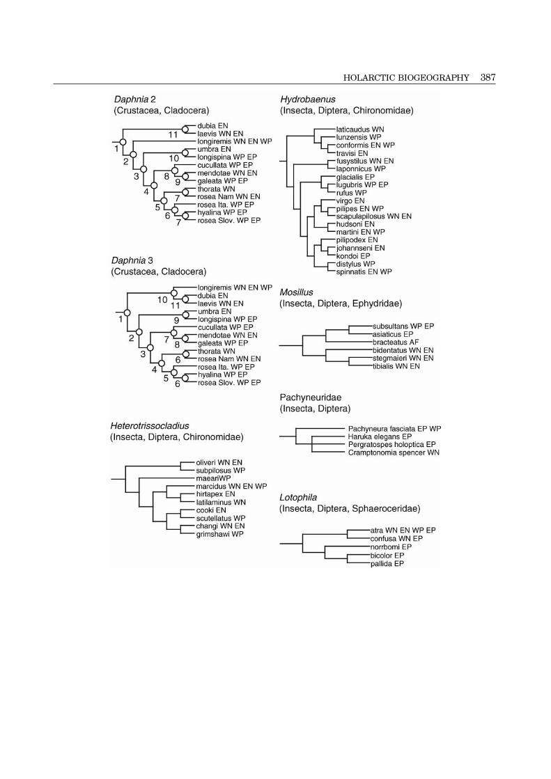
HOLARCTIC BIOGEOGRAPHY 387

388 I. SANMARTIN ET AL.

HOLARCTIC BIOGEOGRAPHY 389

390 I. SANMARTIN ET AL.