.

Ecology, 80(5), 1999, pp. 1475-14940 1999 by the Ecologacal Society of America

SEED DISPERSAL NEAR AND FAR: PATTERNS ACROSS TEMPERATEAND TROPICAL FORESTS

JAMES S.CLARK,' MILES SILMAN,~ RUTH KERN,~ ERIC MACKLIN,~ AND JANNEKE HILLERISLAMBERSI

‘Department of Botany, Duke University, Durham, North Carolina 27708 USA2Smithsonian Tropical Research Institute, Unit 0948, APO AA 34002-0948 USA

‘Harvard Forest, Harvard University, P.O. Box 68, Petersham, Massachusetts 01366 USA4Department of Organismic and Evolutionary Biology, Harvard University, 16 Divinity Avenue, Box 114,

Cambridge, Massachusetts 02138 USA

Abstract. Dispersal affects community dynamics and vegetation response to globalchange. Understanding these effects requires descriptions of dispersal at local and regionalscales and statistical models that permit estimation. Classical models of dispersal describelocal or long-distance dispersal, but not both. The lack of statistical methods means..thatmodels have rarely been fitted to seed dispersal in closed forests. We present a mixturemodel of dispersal that assumes a range of disperal patterns, both local’and long distance.The bivariate Student’s t or “2Dt” follows from an assumption that the distance parameterin a Gaussian model varies randomly, thus having a density of its own. We use an inverseapproach to “compete” our mixture model against classical alternatives, using seed raindatabases from temperate broadleaf, temperate mixed-conifer, and tropical floodplain for-ests. For most species, the 2Dt model fits dispersal data better than do classical models.The superior fit results from the potential for a convex shape near the source tree and a“fat tail.” Our parameter estimates have implications for community dynamics at localscales, for vegetation responses to global change at regional scales, and for differences inseed dispersal among biomes. The 2Dt model predicts that less seed travels beyond theimmediate crown influence (<5 m) than is predicted under a Gaussian model, but that moreseed travels longer distances (>30 m). Although Gaussian and exponential models predictslow population spread in the face of environmental change, our dispersal estimates suggestrapid spread. The preponderance of animal-dispersed and rare seed types in tropical forestsresults in noisier patterns of dispersal than occur in temperate hardwood and conifer stands.

Key words: Bayesian analysis; dispersal kernel: exponential model; forest dynamics; gamma;Gaussian model; migration; seed dispersal; seed shadow: Student’s t.

An understanding of dispersal is needed to assessrecruitment limitation in plant communities and to pre-dict population, responses to global change (Schupp1990, Bibbens et al. 1994, Pitelka et al. 1997, Clark etal. 1998a). Dispersal is summarized by a “seed shad-ow,” describing the density of juveniles with distancefrom the parent. A seed shadow model consists of twoelements: (1) an estimate of fecundity, or the rate ofseed production, and (2) a dispersal “kernel,” or prob-ability density, describing the scatter of that seed about

Manuscript received 2 January 1998; revised 18 August1998; accepted 16 September 1998 .

the parent. The seed shadow is the product of thesetwo elements:

seed shadow = fecundity X dispersal kernel

(1)

Seed shadows describe movement at several spatialscales. At fine scales, the fraction of seed that remainsnear the parent vs. that dispersed broadly affects ag-gregation and, thus, competition (Janzen 1970, Levin1976, Geritz et al. 1984, Levin et al. 1984, Shmida and

..Ellner 1984, Augspurger and Franson 1988, Augspur-ger and Kitajima 1992, Venable and Brown 1993, Hurttand Pacala 1996). At coarse scales, the seed shadowdetermines whether colonization of new habitats occurs

1476 JAMES S. CLARK ET AL. Ecology, Vol.. 80, No. 5 ’ ’

a) Exponential family for Acer Nbfum b) Comparison with 2Dt kernel

nvex under crown

ii

Distance (m)

mostly from patch edges, where seed rain from nearbyadults is dense (Bjorkbom 1971, Hughes and Fahey1988, Greene and Johnson 1989), or from seed trav-eling long distances -(Davis 1981, Ritchie and Mac-Donald .1986? Fastie 1995). Plant migrations during.__ .__.climate change may be controlled by the “tail” of thekernel, with accelerating spread well in advance of thepopulation frontier (Kot et al. 1996, Clark 1998). Takentogether, these observations point to the need for anunderstanding of dispersal both near parent crowns andover long distances.

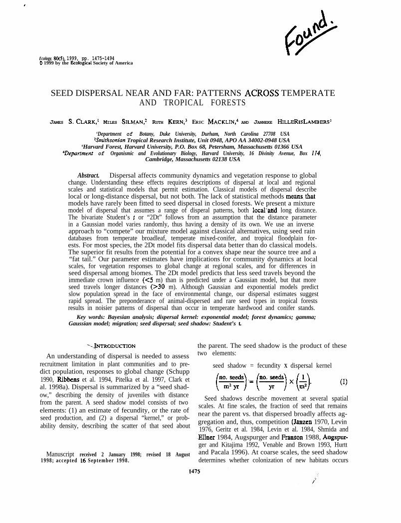
Two challenges stand in the way of predicting dis-persal within natural communities. First is the need forkernel models that accurately describe dispersal acrossa range of spatial scales. The shapes of seed shadowsassumed by dispersal biologists, modelers, and theo-rists reflect focus on a particular scale. Models appliedat a fine scale usually assume a kernel that is convexnear the source and platykurtic (e.g., the Gaussian ker-nel in Fig. la), because this shape describes the influ-ence of the nearby (and sometimes overhanging) can-opy (Green 1983, Geritz et al. 1984, Ribbens et al.1994, Clark &al. 19986). Seed density declines withdistance from the parent tree, slowly’ at first, and thenmore rapidly beyond the crown edge. This “local” con-vexity requires a kernel&r) having a negative secondderivative at the source, @flr)/dr2l+, < 0, where r isdistance (Fig. la). Such dispersal kernels have beenused to estimate probabilities of finding safe sites (Jan-zen 1970, Green 1983, Geritz et al. 1984), competitionwithin tree communities (Ribbens et al. 1994), and re-cruitment limitation (Clark et al. 1998b). The restricteddispersal described by such kernels predicts speciescompositions that can contrast with those from models

,, that assume global .dispersal (Leishman et al. 1992,Hurtt,and Pacala 1993, Ribbens et al. 1994, Clark andJi 1995).

Ecologists concerned with processes that operate at

FIG. 1. Comparison of the shapes of kerneltails fitted to Acer rubrum seed rain. (a) Dif-ferent models in an exponential family (Eq. 3)predict convexity at the source (c > 1) or a fattail (c < l), but not both. Exponential and fat-tailed kernels are more leptokurtic (more peakedand fat tailed) than is the Gaussian. (b) The 2Dtmodel (Eq. 7) predicts convexity at the sourceand a fat tail. Note the log scale of the y-axes.

broad spatial scales, such as reforestation of habitatfragments and population spread, commonly employmodels that are concave near the sou& and leptokurtic(“fat-tailed” in Fig. la). Exponexia densities and -power functions (Portnoy and Wi&on 1993, Willson1993) are examples of models chosen principally forthe shape of the “tail” of the seed shadow, i.e., on seeddispersed beyond the direct crown influence. Relativelysmall differences in the shapes of tails can have largeeffects on rates of population spread (Clark 1998). Pla-tykurtic kernels estimated by dispersal biologists andcommunity ecologists are of little use at coarse scales,whereas the leptokurtic models that appear more rea-sonable at coarse scales are likewise poorly suited forapplication at fine scales.

A second challenge has been the ,development ofstatistical methods for estimation and model testing.Past efforts to describe the scatter of iced about parentplants have enjoyed limited success. Observations fromisolated trees in open or edge situations (Bjorkbom1971, Smith 1975, Carkin et al. 1978, Gladstone 1979,Holthuijzen and Sharik 1985, Lamont 1985, Johnson1988, Greene and Johnson 1989, Guevara and Laborde1993) are hard to generalize to closed forests, becauseexposed crowns have higher seed production and aresubject to different dispersal conditions than are theircounterparts in closed stands (Ruth and Bemtsen 1955,Fowells and Schubert 1956, Barrett 1966, Mair 1973).Seed shadows are a black box in models of stand dy-namics, because there are no obvious ways to measureseed transport in closed canopies where seed shadowsof individual trees overlap (Houle 1992, Martinez-Ra-mos and Soto-Castor 1993). Empirical approaches aresummarized by a collection of functions (reviewed byWillson 1993) that are restricted in application to par-ticular spatial scales and that yield inconsistent fits todata (Portnoy and Willson 1993). Although migrationin response to global change has been critical to species

.

.I

ly 1999 TEMPhATE AND TROPICAL SEED DISPERSAL 1 4 7 7

?rsistence, both past and present, seed dispersal has:t to be incorporated in Dynamic Global Vegetationlodels (DGVMs), because existing empirical models‘e not relevant at coarse scales (Pitelka et al. 1997,lark et al. 1998a).Mechanistic approaches represent an alternative’ap-

roach. Forces that act on an ensemble of seeds, in-uding settling, diffusion, and advection (wind), arele components of Gaussian plume models. Applica-ons to forest community dynamics are limited thustr (we are aware of none), because solutions generally;sume simplistic boundary conditions (e.g., a pointnrrce) and constant wind profile. The distributedu&e, represented by a tree crown or by a stand ofees contributing seed to an open field (Okubo andevin 1989), is responsible for the convex kernel shapelose to that source. The “skip distance” predicted byGaussian plume model with an elevated point sourcend constant wind profile is not expected in real standsrhere winds vary and crowns are broad. Relaxing theisumption of a constant wind profile requires manyammeters that are difficult to obtain and are dependentn specific--conditions (Sharpe and Fields 1982, An-ersen 1991).Inverse modeling represents a powerful methodol-

gy for estimating fecundity and dispersal (Ribbens eti. 1994, Clark et al. 1998a, b). The approach uses theJatial pattern of seed recovered from seed traps anddult trees to statistically estimate the seed shadow.lthough the transport of individual seeds is not ob-zrved, the model of seed arrival in traps can be in-erted to provide parameter estimates, to estimateoodness-of-fit, and to propagate error. The method-logy itself is quite general, accommodating a rangef assumptions regarding kernel shape and error dis-ibution. Alternative views of dispersal are representedy competing functional forms that can be comparedased on field data.Here, we integrate notions of dispersal that cut across

patial scales, and we determine the extent to which alassical vs. a new model derived from this integratediew explains disPersa1 in three biomes. The novel as-umption of our model is that of a seed shadow con-tituting a continuous range of dispersal processes, in-luding ones responsible for local (e.g., settling underonditions of light winds) to long-distance (e.g., move-rent by strong winds and transport by vertebrates) dis-ersal. This assumption is incorporated by modifyingstandard dispersal model to include a density of dis-

,ersal parameters, with the resultant, new seed shadoweing a “continuous mixture.” The resultant mixturerode1 has desirable features at both local (i.e., con-exity near the source) and long (i.e., high kurtosis, orfat tail) distances. We then apply an inverse approach

3 parameterize the model, and we “compete” thislode1 against the classical alternatives using data asrbitrator. Our tests are based on data from southernippalachian, Sierra Nevada mixed-conifer, and Peru-

vian tropical floodplain forests. Comparisons demon-strate commonalities and differences across these con-trasting biomes.

A FIELD GUIDE TO SEED SHADOWS

A brief background summarizes differences amongthe dispersal kernels used to model dispersal, devel-opment of our new kernel, and inferences that can bedrawn from our competitions among kernels using aninverse approach. We begin by describing a kernel intwo dimensions, because this is a source of confusionin the literature.

A dispersal kernel in two dimensions

A tree’s “seed shadow,” the flux of seeds at distancer (in meters), is the product of seed production rate Q(per year) and a density function, or kemelflr, 4):

s(r, 4) = Qifr, 4) (2)

where + is direction (e.g., radians), andflr, 4) is seeddensity per square meter; Eq. 2 is a restatement of Eq.1. We assume rotational symmetry, so direction 4 iseventually suppressed; it is explicit initially to assure -that we arrive at a proper normalization constant (ascalar guaranteeing that all seeds land somewhere). Theprobability that a seed originating at r = 0 falls on anarea of ground surface (or in a seed trap) with diameterdr and subtending arc angle 8 is the integral

rcdr

I ff(r’; +) d+ dr’ = 8

r 9 I

r + d r

r’f,(r’)dr’r

= fhf(r, 4) dr. (3)

Note that integration offir, 4) over arc angle 8 yieldsBr&(r). Integration over both 8 and r yields a dimen-sionless fraction, which, upon multiplication by fecun-dity, gives the annual seed flux (i.e., number of seedsper year) to the area (0, dr). This result is not the seedshadow of Eq. 2, which is a density and has units ofnumber of seeds per square meter per year (Eq. l), but,rather, the integration of it. The integration over 21r is2w-&,(r), which is the marginal density for the randomvariable r. Moments represent a convenient summaryof r and are solved in Appendix A. To simplify notation,we hereafter represent Ar, 4) as fir).

A family of dispersal kernels

Many functional forms can be, and have been, usedto describe how offspring abundances vary with dis-tance from the parent tree. We limit consideration hereto proper density functions. We do not consider powerfunctions, for example, because they contain a singu-larity (infinite density at zero); they cannot be parame-terized to yield finite moments.

Many previous models and the new model developedhere can be placed within the general context of oneanalyzed by Clark et al. (19986):

1 4 7 8 JAMES S. CLARK ET AL. Ecology, Vol. 80, No. 5

f(r) = dexp - ; =lo1 (4)

where a is a distance parameter (in meters), c is adimensionless shape parameter, N is the normalizationconstant,

and

w = z”-‘P dz

is the gamma function. The kernel can be concave atthe source and fat tailed (c.5 1) or convex at the sourceand platykurtic (c > 1). The exponential (c = 1) ismost common:

f(r) = &exp -d .I 1 CW

Alternative kernels in this family include the Gaussiancc = 3,

f(r) = sexp - d ’ .IO1

(5b)

Clark et al. (1998a) and various others; Ribbens et al.(1994) use c = 3, and Kot et al. (1996) and Clark (1998)use c = l/2. Kurtosis, summarized from the second andfourth moments of the marginal density of r,

FR’ I-(6/c)I’(2/c)-=I+ l-9(4/c)

(6)

(see Appendix A), tends to infinity as c tends to zeroand to zero as c becomes large. Thus, Eq. 4 accom-modates the large kurtotsis that power functions at-tempt to capture, while still qualifying as a proper den-sity function.

There are two limitations of dispersal kernels basedon Eq. 4. First, although flexible (e.g., zero to infinitekurtosis), th&eed shadow can be either convex at thesource or leptokurtic, but not both (Fig. la). Second,statistical models used to fit kernels from seed or seed-ling data become unstable if estimation of a and c isattempted simultaneously. For five stands analyzed byClark et al. (1998b), it was necessary to assume a valueof c and then fit a. Ribbens et al. (1994) report similardifficulties. A more flexible kernel is obtained with atwo-part model having “local” and “long-distance”components. The likelihood for this two-part model isill-conditioned, however, prohibiting direct parameterestimation of the long-distance component (Clark 1998).

THE RIGHT SHAPE NEAR AND FAR:A CONTINUOUS MIXTURE

A kernel that accurately describes dispersal at bothlocal and long-distance scales is obtained by charac-

terizing the seed shadow as a composite process, sum-marized by a continuous range of dispersal parametersa. The Gaussian kernel (Eq. 5b) is a reasonable modelfor a restricted set of conditions. The model fits fielddata for most of the tree species that we tested, andspecies differences in dispersal parameters a matchedclosely the predictions based on fall velocities (Clarket al. 1998b). Nonetheless, the model is most sensitiveto seeds dispersed over short distances, and it fails todescribe sporadic seed dispersed over long distances:the tail of the kernel is essentially overlooked.

We modified the Gaussian kernel (Eq. 5b) by assum-ing that it varies continuously with prevailing condi-tions. For example, a small value of a might describethe kernel for seed released during times of light winds,whereas a large value might apply when winds are high,or for seeds dispersed by frugivorous birds, primates,or other vertebrates. Assuming then that a representsa random variable, we require a density of a values,call itfia), to describe the probability of a values dur-ing seed release or transport. There are two restrictionson our choice for densityfla). First,-it must be flexible.Second, it must have a form such that the product ofAa) and fir 1 a) can be integrated to yield a new kernelfir) that incorporates variability in a. In other words,we must be able to solve for the marginal densityflr)that results from the jointly distributed random vari-ables r and a.

We searched for a density f(a) that is both flexibleand permits a solution to (marginal density for) Eq. 5b.Such a solution is obtained by introducing a new vari-able A, that is defined in terms of a and scaling pa-rameter u,

where A is gamma-distributed with shape parameter p:

f(A; p) = ‘s.

Writing Eq. 5b as a density fir IA) conditioned on therandom variable A (which depends, in turn, on a), thenew kernel becomes

f(r (A)f(A) dA = ’ r2 P+l. (8)

7Fu1+-I 1U1 1

A resealing of parameters would show this to be abivariate version of Student’s t distribution. The densityis two dimensional, because the normalization constantincludes the arc-wise integration. Rotational symmetrysuppresses arc angle, but the density is expressed persquare meter rather than per meter. We therefore referto this mixture as a “two-dimensional f”,(2Dt) kernel.It tends to a Gaussian as p becomes large, and to aCauchy as p tends to zero.

Advantages of our 2Dt mixture over variants on Eq.i are threefold. First, it has the right shape at local andong distances. Although convex at the source, it ac-,ommodates both fat and exponentially bounded tails.doments <2p are finite (Appendix A); thus, all mo-nents are finite in the Gaussian limit (p + co), and allIre infinite in the Cauchy limit (p + 0). Kurtosis (in-rolving the fourth moment) is finite for p > 2.

A second advantage of the 2Dt distribution is theact that the density of IX is obtained as a by-product)f fitting the kernel itself. Rather than simply obtainingjest estimates of Q and confidence intervals (e.g., Clarkt al. 19986), we obtain a full density of dispersal val-[es with the variable change:

f(a) = f(A) 2 = atifz(p)exp - $, .I I 1 1 (9)

:his density can be viewed as a type of inverse x2./laments of 01 can be expressed in terms of the mo-aents of the kernel itself:

Fe =2Piim

mr(ml2) *

‘hese moments are finite so long as the corresponding.loments of the kernel are finite. Thus, the mean of (Y; 1.12 times as large as the mean dispersal distance.‘he mode, which obtains at d lnAa)/da = 0, is

d 2 u 0 lo 20 30 40 50 60#amodc =

2p+ 1’Distance (m)

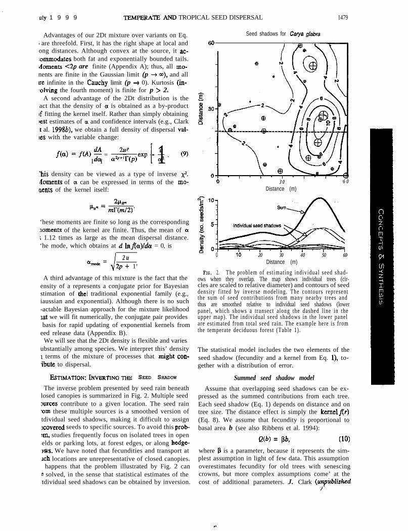
FIG. 2.A third advantage of this mixture is the fact that the

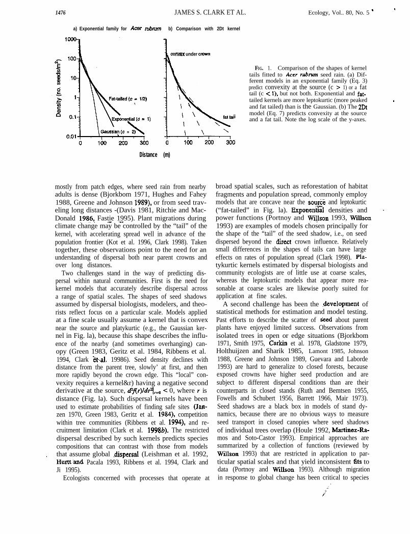
The problem of est imating individual seed shad-ows when they overlap. The map shows individual trees (cir-

ensity of a represents a conjugate prior for Bayesian cles are scaled to relative diameter) and contours of seedstimation of the’ traditional exponential family (e.g., density f i t ted by inverse modeling. The contours representiaussian and exponential). Although there is no such the sum of seed contributions from many nearby trees and

-actable Bayesian approach for the mixture likelihoodthus are smoothed relative to individual seed shadows (lowerpanel, which shows a transect along the dashed l ine in the

Iat we will fit numerically, the conjugate pair provides upper map). The individual seed shadows in the lower panelbasis for rapid updating of exponential kernels from are estimated from total seed rain. The example here is from

eed release data (Appendix B). the temperate deciduous forest (Table 1).

We will see that the 2Dt density is flexible and variesubstantially among species. We interpret this’ density The statistical model includes the two elements of thet terms of the mixture of processes that .might con- seed shadow (fecundity and a kernel from Eq. l), to-ibute to dispersal. gether with a distribution of error.

ESTIMATION:~NVERTINGTHE SEED SHADOW Summed seed shadow modelThe inverse problem presented by seed rain beneath Assume that overlapping seed shadows can be ex-

losed canopies is summarized in Fig. 2. Multiple seed pressed as the summed contributions from each tree.>urces contribute to a given location. The seed rain Each seed shadow (Eq. 1) depends on distance and on-om these multiple sources is a smoothed version of tree size. The distance effect is simply the kernelflr)tdividual seed shadows, making it difficult to assign (Eq. 8). We assume that fecundity is proportional to:covered seeds to specific sources. To avoid this prob- basal area b (see also Ribbens et al. 1994)::m, studies frequently focus on isolated trees in openelds or parking lots, at forest edges, or along hedge- Q(b) = Bh (10))ws. We have noted that fecundities and transport at where B is a parameter, because it represents the sim-lch locations are unrepresentative of closed canopies. plest assumption in light of few data. This assumption

happens that the problem illustrated by Fig. 2 can overestimates fecundity for old trees with senescinge solved, in the sense that statistical estimates of the crowns, but more complex assumptions come’ at thetdividual seed shadows can be obtained by inversion. cost of additional parameters. J. Clark (unpubZished

?

TBMPERATE AND TROPICAL SEED DISPERSAL 1479

Seed shadows for Carya glabra

1

3 0Distance (m)

6 0

.uly 1 9 9 9

1480 JAMES S. CLARK ET AL. Ecology, Vol. 80, No. 5

TABLE 1. Forest stands used to model dispersal.

Forest type(location)

Annualprecipitation Elevation Dominant species

(mm) b-4 Stand number, type (based on basal area)

Temperate mixed-conifer(36”34’ N, 118”46’ W)

870

1090

1390

1000 2200

2200

Temperate deciduous 1900 790(35’03’ N, 83”27’ W)

800

1600

1600

Tropical floodplain 2000 350(1 lo54 S, 71”22’ W)

1,

2,

3,

4 ,

5,

1,

2,

3 ,

4 .

xeric ridge

cove hardwood

mixed oak

mixed oak

northern hardwood

Sierra Nevada mixed-conifer

sequoia-mixed-conifer

Sierra Nevada mixed-conifer

Sierra Nevada mixed-conifer

Quercus spp., Pinus rigida, Acerrubrum

Liriodendron tulipifera, Quercusspp., Acer rubrum

Quercus spp., Acer rubrum, Catyaglabra

Quercus spp., Acer rubrum, Nyssasylvatica

Betula spp., Quercus spp., Tiliaamericana

Abies concolor, Abies magnijcavar. shastensis, Sequoiadendrongiganteum

Sequoiadendron giganteum, Abiesconcolor, Abies magnijca var.shastensis

Calocedrus decurrens, Abiesconcolor, Quercus kelloggii

Calocedrus decurrens, Quercuskelloggii, Pinus ponderosa

Otoba parvifolia;-Quararibea witti

manuscript) is examining nonlinear fecundity modelsfor one of our data sets. In most cases, Eq. 10 fits thedata better than do more complex assumptions.

The model of seed rain is the sum of individual seedshadows in Eq. 2. Using functional forms for Q (Eq.10) andflr) (Eq. 8), we write the summed model as

(11)

where 3(b, rj; ‘pZ) is the seed density predicted at seedtrap j, based on an m-length vector of tree basal areasb, an m X n matrix of distances r, and a vector of zfitted parameters, which, for the 2Dt model in Eq. 8,is qr = [p, u, p]. We find parameter values that fit the“sum” in Fig. 2, which, by implication, allows us todraw the “individual seed shadows” that together de-fine that sums..

Likelihood: data and distribution of errorAssuming a model, the likelihood of obtaining a data

set is the joint likelihood (i.e., product) of observingeach datum. Our data consist of mapped tree plots withseed traps in three forests (Table 1). Stand composition,dispersal biology, and data sets are described elsewhere(Clark et al. 19986; M. Silman and J. Clark, unpub-

TABLE 2. Summary of data sets analyzed in this study.

lished manuscript; R. Kern et al., unpublished manu-script). In brief, mapped stands include the location(coordinates), diameter at breast height, and species ofeach tree. The finite areas of our maps (Table 2) canaffect parameter estimates for the best dispersed spe-cies (Betulu, Liriodendron) only on our smallest plots,those from the southern Appalachians (Clark et al.1998b). Seeds were identified to the lowest possibletaxonomic unit and were expressed as density per year.Each datum is the seed accumulation in one seed trap,averaged over the duration of the study (Table 2).

Seed traps do not receive precisely the number ofseeds predicted by Eq. 11, but rather some stochasticrealization of it. The error distribution describes thescatter of seed densit ies about the mean value predictedby the seed shadow. Clark et al. (19986) used a negativebinomial, because seed rain was found to be moreclumped than a Poisson distribution. The negative bi-nomial permits this clumping at the cost of an extrafitted parameter. Because our mixture kernel introducesa random variable (IX) that tends to accommodate ad-ditional variability, our attempts to fit the 2Dt kernelwith negative binomial error resulted in unstable pa-rameter estimates. We therefore use the Poisson like-lihood:

.

Area of each stand No. seed traps Area per seed trap, - ’ Forest type No. stands (q) (ha) per stand Cm*) Duration (yr)

Temperate deciduous 5 0.36 20 0.18Temperate mixed-conifer 4 1.0-2.5 0.25 i 354tTropic floodplain 1 2.25 :z 0.50 2

t Durations of seed collections were four years in stand 1 and three years in all others. , ,z

July 1999 TEMPERATE AND TROPICAL SEED DISPERSAL 1481

j-l S,!

where S is an n-length vector of observed seed densities(seed trap counts), and sj is the observed density ofseed in trap j. Although we do not observe the travelfrom trees to seed traps, the likelihood (Eq. 12) pro-vides a means for “inverting” the problem and, thus,estimating parameters.

Parameter estimation for the alternative dispersalmodels (Eqs. 5a, b, 8) follows Clark et al. (19986). Weoutline the approach for the 2Dt kernel, because similarmethodology applies to the exponential (5a) and Gauss-ian (5b) models. Maximum likelihood (ML) estimatesfor the parameter vector cp = [a, 8, p] maximize thelikelihood of observing data set S (Eq. 12), given themodel represented by Eq. 11. In numerically minimiz-ing Eq. 12, we constrained our search for p estimateson the interval (l/2, lo), because a tendency for cor-relation between parameters p and ‘u in bootstrappedestimates outside this range became severe. In mostcases, fitted p values tended to low values (l/2), in-dicating a fat-tailed kernel. Less frequently, p tendedto high values, or a Gaussian kernel. We determined95% confidence intervals on parameters, and we prop-agated error through the seed shadow s(r) and the den-sity of OL values, Jo). We bootstrapped 500 estimateson resamples (with replacement) from seed traps, andwe constructed corresponding s(r) and fro) functionsfor each resample. Our method is Efron and Tibshir-ani’s (1993) “nonparametric” bootstrap; we sample di-rectly from the data rather than from a parametric dis-tribution. Confidence intervals are 95% quantiles ofeach parameter and at l-m intervals forflr) and j(o).Clark et al. (1998b) found that bias-corrected and ac-celerated confidence intervals (Efron and Tishirani1993) did not differ substantially from simple boot-strapped quantiles, so we report quantiles here. Con-fidence intervals about the functions s(r) andflol) prop-agate parameter error and correlation through to theconfidence in the seed shadow and in the density ofdispersal variables.

We estimated $rameters for one to several standsfor data sets having more than one stand (temperatedeciduous and temperate mixed-conifer). Some specieswere too rare to obtain fits in all stands. In a few cases,trees were so abundant that seed rain was too uniformacross plots to permit parameter estimates. Thus, eachfit is obtained on q 5 5 (temperate deciduous) or q 54 (temperate mixed-conifer) stands, with the likelihood

us, I Q) = qaq L(S, 1 Q). (13)

L(S,I cp) is the likelihood of the data observed in thekth stand (Eq. 12). The vector of fitted parameters cpdepends on q and on one of several hypotheses that wetested from our data. We report a weighted rZ as agoodness-of-fit index, where weights are variance es-

timates taken as the predicted mean for this Poissonmodel.

Which model is best?

Hypothesis tests were used to assess parameter con-sistency and to guide model selection. Data were usedto arbitrate among three competing models (Gaussian,exponential, and 2Dt) on the basis of likelihoods. TheGaussian model (parameter vector cp = [p, IX]) is nestedwithin the 2Dt model, being obtained in the limit as pbecomes large. Although nested, the classical likeli-hood ratio test with 1 df is not quite correct. Becausethe Gaussian ,obtains at the boundary p + 03, the like-lihood ratio is a mixture of x2 distributions having 0and 1 df, each with probability l/2, the former beinga delta function centered on zero (Chernoff 1954).Probabilities for our comparisons of Gaussian vs. 2Dtuse this mixed distribution.

The exponential model (parameter vector Q = [8, 011)differs from the Gaussian only in the value of the ex-ponent (c in Eq. 4), so the best fitting model is thathaving the lowest -1n L. For comparing the “gener-alized exponential” and 2Dt models, we treated pa-rameter c in Eq. 4 as a fitted parameter to give param-eter vector Q = [p, o, c]. These two models are notnested, but they contain the same number of parameters(3); the best fitting model is simply the one with thelowest -In L. Our parameter search for c was boundedon (1,4), because parameter correlations became severefor c < 1, and likelihoods were insensitive to valuesof c > 4.

Hypothesis tests for goodness-of-fit

Hypothesis testing for the 2Dt kernel follows Clarket al. (1998b). Provided that parameters (and the seedshadows they represent) are consistent from stand tostand, the most general parameter estimates come whenfitted simultaneously to all stands having sufficienttrees and seeds of a species. Three parameters representthe fits obtained when all possible information is in-cluded:

P3 = us 4 PI. (14)

The null model is simply the Poisson, where each seedtrap receives the mean density. The deviance

(15)

is distributed as x2 with 2 degrees of freedom, threeparameters for the fitted model minus one (the mean)for the null Poisson.

Although Eq. 14 includes the maximum informationon the seed shadow for a species, we tested whetherdispersal differs among plots by comparing this “glob-al” seed shadow with the likelihood of the data underthe hypothesis of q different seed shadows (i.e., a seedshadow differs from plot to plot) with parameter vector

1482 JAMES S. CLARK ET AL. Ecology, Vol. 80, No. 5

P%+I = [P,, . * * , Pqr Ulr . . . 9 ug, PI. (16)

The hypothesis of q different seed shadows is testedusing the likelihood ratio test, where the deviance

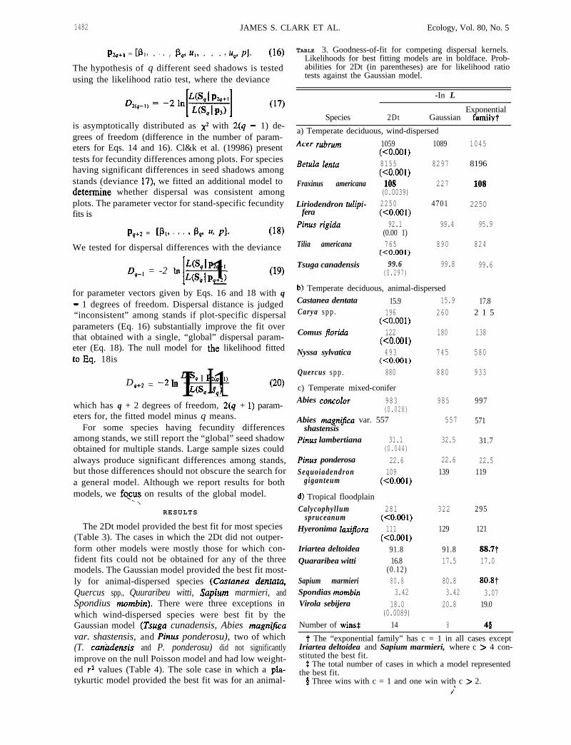
TABLE 3. Goodness-of-fit for competing dispersal kernels.Likelihoods for best fitting models are in boldface. Prob-abilities for 2Dt (in parentheses) are for likelihood ratiotests against the Gaussian model.

is asymptotically distributed as x2 with 2(q - 1) de-grees of freedom (difference in the number of param-eters for Eqs. 14 and 16). Cl&k et al. (19986) presenttests for fecundity differences among plots. For specieshaving significant differences in seed shadows amongstands (deviance 17), we fitted an additional model to,determine whether dispersal was consistent amongplots. The parameter vector for stand-specific fecundityfits is

Pp+* = h * * * 9 pqr w PI. (18)

We tested for dispersal differences with the deviance

D,-, = -2 ln ;:ss’/F;i 1 (19)4 q+*

for parameter vectors given by Eqs. 16 and 18 with q- 1 degrees of freedom. Dispersal distance is judged“inconsistent” among stands if plot-specific dispersalparameters (Eq. 16) substantially improve the fit overthat obtained with a single, “global” dispersal param-eter (Eq. 18). The null model for the likelihood fittedtoEq. 18is

Dq+2 =-2 ln L(S, I PXq+I)I 1us, I fq9) (20)

which has q + 2 degrees of freedom, 2(q + 1) param-eters for, the fitted model minus q means.

For some species having fecundity differencesamong stands, we still report the “global” seed shadowobtained for multiple stands. Large sample sizes couldalways produce significant differences among stands,but those differences should not obscure the search fora general model. Although we report results for bothmodels, we fosus on results of the global model.

\RESULTS

The 2Dt model provided the best fit for most species(Table 3). The cases in which the 2Dt did not outper-form other models were mostly those for which con-fident fits could not be obtained for any of the threemodels. The Gaussian model provided the best fit most-ly for animal-dispersed species (Cusfanea dentutu,Quercus spp., Quuraribeu witti, Supium marmieri, andSpondius mombin). There were three exceptions inwhich wind-dispersed species were best fit by theGaussian model (Tsugu cunadensis, Abies magnificuvar. shastensis, and Pinus ponderosu), two of which(T. cukdensis and P. ponderosu) did not significantlyimprove on the null Poisson model and had low weight-ed r* values (Table 4). The sole case in which a pla-tykurtic model provided the best fit was for an animal-

-In L

Species 2DtExponential

Gaussian family?a) Temperate deciduous, wind-dispersedAcer rubrum 1059 1089

(<O.OOl)Bet&a lenta 8155 8297

(CO.001)Fraxinus americana 10s 227

(0.0039)Liriodendron tulipi- 2250 4701

fera (<O.OOl)Pinus rigida 92.1 99.4

(0.00 1)Tilia americana 765 890

(<O.OOl)Tsuga canadensis 99.6 99.8

(0.297)

b) Temperate deciduous, animal-dispersedCastanea dentata 15.9Carya spp . 196

(<O.OOl)Comus jlorida 122

(<O.OOl)Nyssa sylvatica 493

(<O.OOl)Quercus spp . 880

c) Temperate mixed-coniferAbies concolor 983

(0.028)Abies magnijca var. 557

shastensisPinus lambertiana 31.1

(0.044)Pinus ponderosa 22.6Sequoiadendron 109

giganteum (CO.001)

d) Tropical floodplainCalycophyllum 281

spruceanum (<O.OOl)Hyeronima laxijora 111

(<O.OOl)Iriartea deltoidea 91.8Quararibea witti 16.8

(0.12)Sapium marmieri 80.8Spondias mombin 3.42Virola sebijera 18.0

(0.0089)Number of wins* 14

15.9 17.8260 2 1 5

180 138

745 580

880 933

985 997

557 571

32.5 31.7

22.6 22.5139 119

322

129

91.8 88.7t17.5 17.0

80.8 80.8t3.42 3.07

20.8 19.0

8

1045

8196

10s

2250

95.9

824

99.6

295

121

4st The “exponential family” has c = 1 in all cases except

Iriartea deltoidea and Sapium marmieri, where c > 4 con-stituted the best fit.

$ The total number of cases in which a model representedthe best fit.

8 Three wins with c = 1 and one win with c > 2.$5

July 1999 TEMPERATE @ TROPICAL SEED DISPERSAL 1483

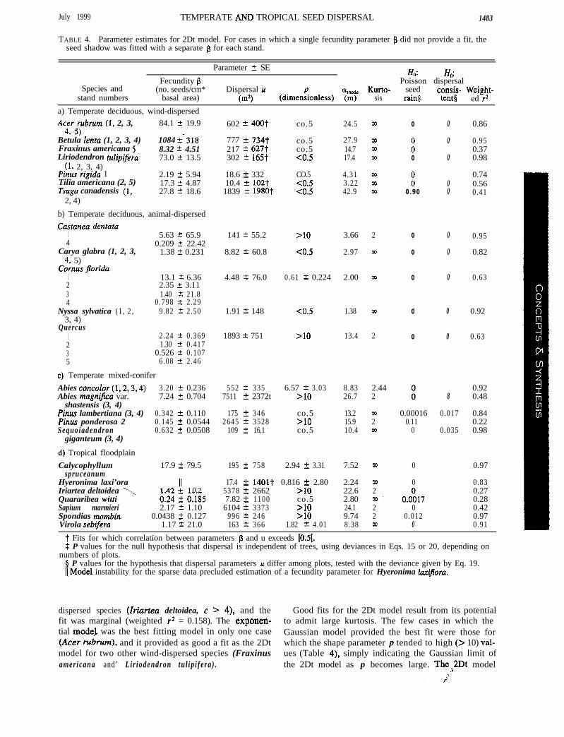
TABLE 4. Parameter estimates for 2Dt model. For cases in which a single fecundity parameter fi did not provide a fit, theseed shadow was fitted with a separate p for each stand.

Species andstand numbers

Parameter t SE Ho: H,:Fecundity p Poisson dispersal

(no. seeds/cm* Dispersal u(dimenzonless) 57

Kurto- seed consis- Weight-basal area) WI sis rain8 tent8 ed rz

a) Temperate deciduous, wind-dispersedAcer rubrum (1, 2, 3, 84.1 t 19.9

4, 5)Betula lenta (1, 2, 3, 4) 1084 i’318Fraxinus americana 5 8.32 If: 4.51Liriodendron tulipifera 73.0 t 13.5

(1, 2, 3, 4)Pinus rigida 1 2.19 c 5.94Tilia americana (2, 5) 17.3 f 4.87Tsuga canadensis (I, 27.8 + 18.6

2, 4)

b) Temperate deciduous, animal-dispersedCastanea dentata

1 5.63 ” 65.94 0.209 2 22.42

Carya glabra (1, 2, 3, 1.38 + 0.2314, 5)

Cornus florida1 13.1 k 6.362 2.35 2 3.113 1.40 t 21.84 0.798 2 2.29

Nyssa sylvatica (1 , 2 , 9.82 t 2.503, 4)

Quercus1 2 .24 t 0.3692 1.30 ” 0.4173 0.526 + 0.1075 6.08 t 2.46

c) Temperate mixed-coniferAbies concoEor (1,2,3,4)Abies magnifica var.

shastensis (3, 4)Pinus lambertiana (3, 4)Pinus ponderosa 2Sequoiadendron

giganteum (3, 4)

d) Tropical floodplainCalycophyllum

spruceanumHyeronima laxi’oraIriartea deltoidea ---.,Quararibea wittiSapium marmieriSpondias mombinVirola sebifera

3.20 2 0.236 552 + 3357.24 -c 0.704 7511 k 2372t

0.342 ” 0.110 175 2 3460.145 c 0.0544 2645 ‘- 35280.632 2 0.0508 109 + 16.1

17.9 + 79.5

142! 1020:24 It O.i852.17 2 1.10

0.0438 + 0.1271.17 2 21.0

602 -c 400t

777 t 734t217 rt 627t302 2 165t

18.6 -c 33210.4 t 102t1839 2 1980t

141 + 55.2

8.82 2 60.8

>lO

<OS

4.48 2 76.0 0.61 2 0.224

1.91 2 148

1893 2 751

195 ” 758 2.94 2 3.31

17.4 2 1401t 0.816 + 2.805378 2 2662 >I07.82 2 1100 co.56104 t 3373 >lO

996 2 246 >lO163 2 366 1.82 + 4.01

co.5

co.5co.5co.5

CO.5CO.5co.5

CO.5

>I0

6.57 2 3.03>lO

co.5>lOco.5

24.5 CQ

27.9 m14.7 m17.4 m

4.31 m3.22 0042.9 02

3.66 2

2.97 m

2.00 m

1.38 m

13.4 2

8.83 2.4426.7 2

13.2 m15.9 210.4 m

7.52 00

2.24 0322.6 22.80 m ’24.1 29.74 28.38 TV

0

:0

:0 . 9 0

0

0

0

0

0

0.000160.11

0

0

0

0.00ol70

0.012

0

0

0

00

0

0

0

0

0

8

0.017

0.035

0.86

0.950.370.98

0.740.560.41

0.95

0.82

0.63

0.92

0.63

0.920.48

0.840.220.98

0.97

0.830.270.280.420.97

0 0.91

t Fits for which correlation between parameters S and u exceeds 10.51.$ P values for the null hypothesis that dispersal is independent of trees, using deviances in Eqs. 15 or 20, depending on

numbers of plots.0 P values for the hypothesis that dispersal parameters u differ among plots, tested with the deviance given by Eq. 19.Il,Model instability for the sparse data precluded estimation of a fecundity parameter for Hyeronima ZaxiJlora.

dispersed species (Zriartea deltoidea, c > 4), and the Good fits for the 2Dt model result from its potentialfit was marginal (weighted r2 = 0.158). The exponen- to admit large kurtosis. The few cases in which thetial model was the best fitting model in only one case Gaussian model provided the best fit were those for(Acer rulirum), and it provided as good a fit as the 2Dt which the shape parameter p tended to high (> 10) val-model for two other wind-dispersed species (Fraxinus ues (Table 4), simply indicating the Gaussian limit ofamericana and’ Lir iodendron tul ip i fera) . the 2Dt model as p becomes large. Thei2Dt model

1484 JAMES S. CLARK ET AL. Ecology, Vol. 80, No. 5

a) Sequoiadendron giganteum seed shadow b) Density of c1 values (2Dt)

A

1 G a u s s i a n / l OAM1

6 0 3 0 0 3 0 6 0 0 5 0 1 0 0

Distance (m)

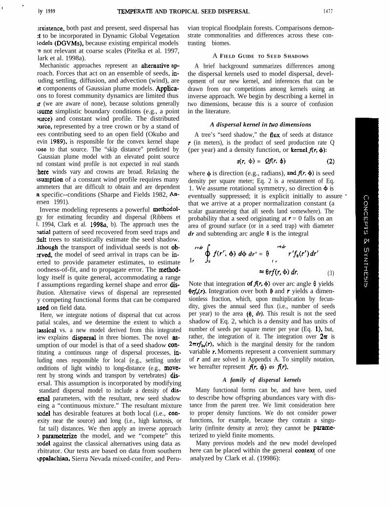
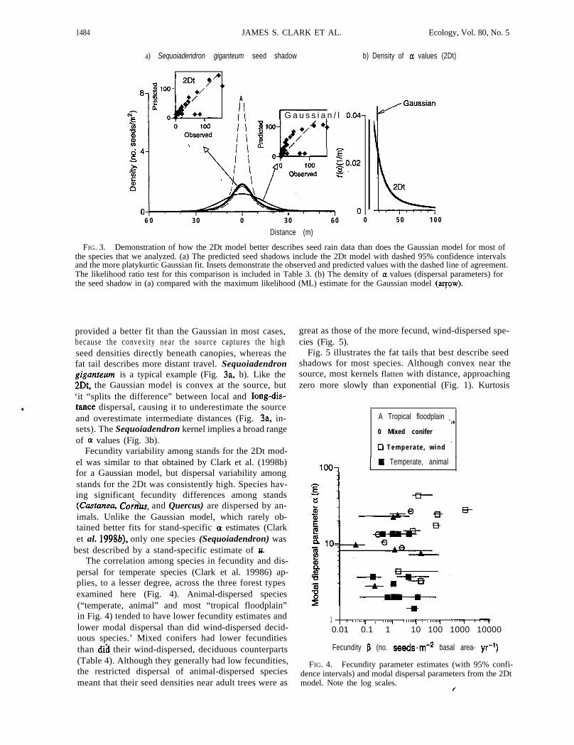
FIG. 3. Demonstration of how the 2Dt model better describes seed rain data than does the Gaussian model for most ofthe species that we analyzed. (a) The predicted seed shadows include the 2Dt model with dashed 95% confidence intervalsand the more platykurtic Gaussian fit. Insets demonstrate the observed and predicted values with the dashed line of agreement.The likelihood ratio test for this comparison is included in Table 3. (b) The density of CL values (dispersal parameters) forthe seed shadow in (a) compared with the maximum likelihood (ML) estimate for the Gaussian model (aryow).

provided a better fit than the Gaussian in most cases, great as those of the more fecund, wind-dispersed spe-cies (Fig. 5).because the convexity near the source captures the high

seed densities directly beneath canopies, whereas thefat tail describes more distant travel. Sequoiadendrongiganreum is a typical example (Fig. 3a, b). Like the2Dt, the Gaussian model is convex at the source, but‘it “splits the difference” between local and long-dis-tance dispersal, causing it to underestimate the sourceand overestimate intermediate distances (Fig. 3a, in-sets). The Sequoiadendron kernel implies a broad rangeof OL values (Fig. 3b).

Fecundity variability among stands for the 2Dt mod-el was similar to that obtained by Clark et al. (1998b)for a Gaussian model, but dispersal variability amongstands for the 2Dt was consistently high. Species hav-ing significant fecundity differences among stands(Castanea, Co?&, and Quercus) are dispersed by an-imals. Unlike the Gaussian model, which rarely ob-tained better fits for stand-specific (Y estimates (Clarket al. 1998b), only one species (Sequoiadendron) was

’ best described by a stand-specific estimate of u.The correlation among species in fecundity and dis-

persal for temperate species (Clark et al. 19986) ap-plies, to a lesser degree, across the three forest typesexamined here (Fig. 4). Animal-dispersed species(“temperate, animal” and most “tropical floodplain”in Fig. 4) tended to have lower fecundity estimates andlower modal dispersal than did wind-dispersed decid-uous species.’ Mixed conifers had lower fecunditiesthan di& their wind-dispersed, deciduous counterparts(Table 4). Although they generally had low fecundities,the restricted dispersal of animal-dispersed speciesmeant that their seed densities near adult trees were as

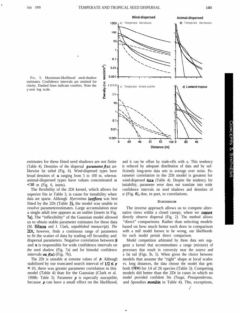
Fig. 5 illustrates the fat tails that best describe seedshadows for most species. Although convex near thesource, most kernels flatten with distance, approachingzero more slowly than exponential (Fig. 1). Kurtosis

A Tropical floodplain ,, .?0 Mixed conifer

0 Tempera te , w ind ’

H Temperate, animal

-m1 I I111111, 4 , 111111, I 1111111, I I1U8188, I I111111, I I “mq0.01 0.1 1 10 100 1000 10000

Fecundity p (no. seedsvm-* basal area- yr-‘)

FIG. 4. Fecundity parameter estimates (with 95% confi-dence intervals) and modal dispersal parameters from the 2Dtmodel. Note the log scales.

i

.July 1999 TEMPERATE AND TROPICAL SEED DISPERSAL

FIG. 5. Maximum-likelihood seed-shadowestimates. Confidence intervals are omitted forclarity. Dashed lines indicate conifers. Note they-axis log scale.

Wind-disperseda ) T e m p e r a t e d e c i d u o u s

z 1 0 0 00

c ) T e m p e r a t e m i x e d - c o n i f e r

Es

1 0 0

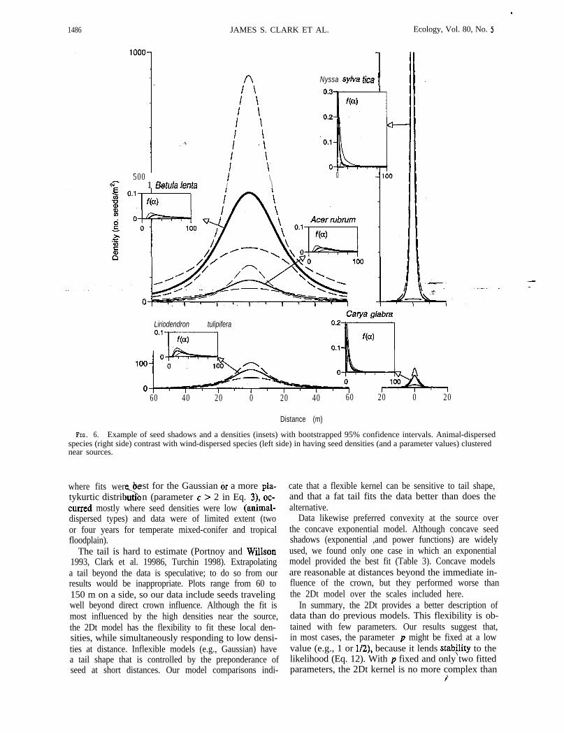
estimates for these fitted seed shadows are not finite(Table 4). Densities of the dispersal parameterffoc) arelikewise fat tailed (Fig. 6). Wind-dispersed types havebroad densities of OL ranging from 5 to 100 m, whereasanimal-dispersed types have values concentrated at<lo m (Fig. 6, insets).

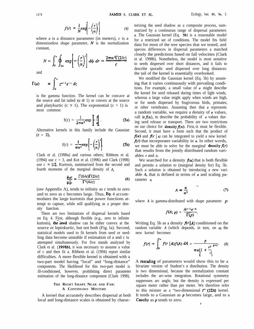
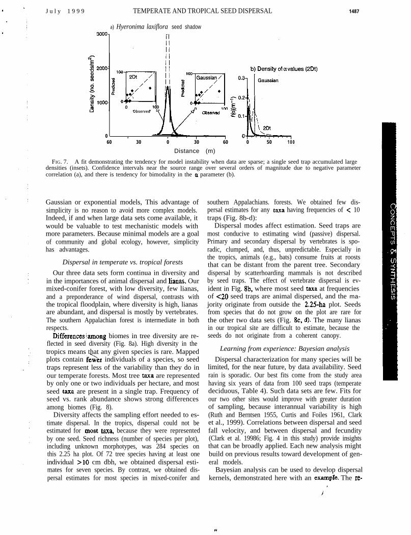
The flexibility of the 2Dt kernel, which allows forsuperior fits in Table 3, is cause for instability whendata are sparse. Although Hyeronima loxifrora was bestfitted by the 2Dt (Table 3), the model was unable toresolve parameterestimates. Large accumulation neara single adult tree appears as an outlier (insets in Fig.7a). The “inflexibility” of the Gaussian model allowedus to obtain stable parameter estimates for these data(M. Silman and J. Clark, unpublished manuscript). The2Dt, however, finds a continuous range of parametersto fit the scatter of data by trading off fecundity anddispersal parameters. Negative correlation between pand OL is responsible for wide confidence intervals onthe seed shadow (Fig. 7a) and for bimodal confidenceintervals onfla) (Fig. 7b).

The 2Dt is unstable at extreme values of p. Althoughstabilized by our truncated search interval of l/2 I p5 10, there was greater parameter correlation in thismodel (Table 4) than for the Gaussian (Clark et al.1998b: Table 3). Parameter p is especially susceptible,because p can have a small effect on the likelihood,

60 60

1485

Animal-dispersed.b) T e m p e r a t e d e c i d u o u s

Distance (m)

and it can be offset by trade-offs with u. This tendencyis reduced by adequate distribution of data and by suf-ficiently long-term data sets to average over noise. Pa-rameter correlation in the 2Dt model is greatest forwind-dispersed taxa (Table 4). Despite the tendency forinstability, parameter error does not translate into wideconfidence intervals on seed shadows and densities ofa (Fig. 6), due, in part, to correlations.

DISCUSSION

The inverse approach allows us to compete alter-native views within a closed canopy, where we cannotdirectly observe dispersal (Fig. 2). The method allows“direct” comparisons. Rather than selecting modelsbased on how much better each does in comparisonwith a null model known to be wrong, our likelihoodsfor each model permit direct comparison.

Model competition arbitrated by three data sets sug-gests a kernel that accommodates a range (mixture) ofprocesses that result in convexity near the source anda fat tail (Figs. lb, 5). When given the choice betweenmodels that assume the “right” shape at local scalesvs. long distances, the data choose the model that getsboth (2Dt) for 14 of 26 species (Table 3). Competingmodels did better than the 2Dt in cases in which nomodel provided confident fits (Tsuga, Pinusponderosa,and Spondias mombin in Table 4). The, exceptions,

i

1486 JAMES S. CLARK ET AL. Ecology, Vol. 80, No. 5

I^\: :I I

Nyssa sylva tica 1

5001

I \ 0Betula lenta I \

Liriodendron tulipiferaCarya glabra

60 40 20 0 20 40 60 20 0 20

Distance (m)

FIG. 6. Example of seed shadows and a densities (insets) with bootstrapped 95% confidence intervals. Animal-dispersedspecies (right side) contrast with wind-dispersed species (left side) in having seed densities (and a parameter values) clusterednear sources.

where fits wer best for the Gaussian c3r a more pla-\tykurtic distributi n (parameter c > 2 in Eq. 3), oc-

curred mostly where seed densities were low (animal-dispersed types) and data were of limited extent (twoor four years for temperate mixed-conifer and tropicalfloodplain).

The tail is hard to estimate (Portnoy and Willson1993, Clark et al. 19986, Turchin 1998). Extrapolatinga tail beyond the data is speculative; to do so from ourresults would be inappropriate. Plots range from 60 to150 m on a side, so our data include seeds travelingwell beyond direct crown influence. Although the fit ismost influenced by the high densities near the source,the 2Dt model has the flexibility to fit these local den-sities, while simultaneously responding to low densi-ties at distance. Inflexible models (e.g., Gaussian) havea tail shape that is controlled by the preponderance ofseed at short distances. Our model comparisons indi-

cate that a flexible kernel can be sensitive to tail shape,and that a fat tail fits the data better than does thealternative.

Data likewise preferred convexity at the source overthe concave exponential model. Although concave seedshadows (exponential ,and power functions) are widelyused, we found only one case in which an exponentialmodel provided the best fit (Table 3). Concave modelsare reasonable at distances beyond the immediate in-fluence of the crown, but they performed worse thanthe 2Dt model over the scales included here.

In summary, the 2Dt provides a better description ofdata than do previous models. This flexibility is ob-tained with few parameters. Our results suggest that,in most cases, the parameter p might be fixed at a lowvalue (e.g., 1 or l/2), because it lends stab<lity to thelikelihood (Eq. 12). With p fixed and only two fittedparameters, the 2Dt kernel is no more complex than

9

J u l y 1 9 9 9 TEMPERATE AND TROPICAL SEED DISPERSAL

a) Hyeronima laxiflora seed shadow

Observed

1487

0 , I ,60 30 0 30 60 0 50 1 0 0

Distance (m)

FIG. 7. A fit demonstrating the tendency for model instability when data are sparse; a single seed trap accumulated largedensities (insets). Confidence intervals near the source range over several orders of magnitude due to negative parametercorrelation (a), and there is tendency for bimodality in the o parameter (b).

Gaussian or exponential models, This advantage ofsimplicity is no reason to avoid more complex models.Indeed, if and when large data sets come available, itwould be valuable to test mechanistic models withmore parameters. Because minimal models are a goalof community and global ecology, however, simplicityhas advantages.

Dispersal in temperate vs. tropical forestsOur three data sets form continua in diversity and

in the importances of animal dispersal and l&as. Ourmixed-conifer forest, with low diversity, few lianas,and a preponderance of wind dispersal, contrasts withthe tropical floodplain, where diversity is high, lianasare abundant, and dispersal is mostly by vertebrates.The southern Appalachian forest is intermediate in bothrespects.

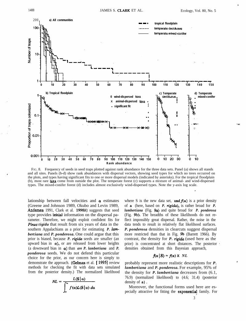
Differenceslamong biomes in tree diversity are re-flected in seed diversity (Fig. 8a). High diversity in thetropics means that any given species is rare. Mappedplots contain fe>er individuals of a species, so seedtraps represent less of the variability than they do inour temperate forests. Most tree taxa are representedby only one or two individuals per hectare, and mostseed taxa are present in a single trap. Frequency ofseed vs. rank abundance shows strong differencesamong biomes (Fig. 8).

Diversity affects the sampling effort needed to es-timate dispersal. In the tropics, dispersal could not beestimated for host taxa, because they were representedby one seed. Seed richness (number of species per plot),including unknown morphotypes, was 284 species onthis 2.25 ha plot. Of 72 tree species having at least oneindividual >lO cm dbh, we obtained dispersal esti-mates for seven species. By contrast, we obtained dis-persal estimates for most species in mixed-conifer and

southern Appalachians. forests. We obtained few dis-persal estimates for any taxa having frequencies of < 10traps (Fig. 8b-d):

Dispersal modes affect estimation. Seed traps aremost conducive to estimating wind (passive) dispersal.Primary and secondary dispersal by vertebrates is spo-radic, clumped, and, thus, unpredictable. Especially inthe tropics, animals (e.g., bats) consume fruits at rooststhat can be distant from the parent tree. Secondarydispersal by scatterhoarding mammals is not describedby seed traps. The effect of vertebrate dispersal is ev-ident in Fig. 8b, where most seed taxa at frequenciesof ~20 seed traps are animal dispersed, and the ma-jority originate from outside the 2.25-ha plot. Seedsfrom species that do not grow on the plot are rare forthe other two data sets (Fig. 8c, d). The many lianasin our tropical site are difficult to estimate, because theseeds do not originate from a coherent canopy.

Learning from experience: Bayesian analysisDispersal characterization for many species will be

limited, for the near future, by data availability. Seedrain is sporadic. Our best fits come from the study areahaving six years of data from 100 seed traps (temperatedeciduous, Table 4). Such data sets are few. Fits forour two other sites would improve with greater durationof sampling, because interannual variability is high(Ruth and Berntsen 1955, Curtis and Foiles 1961, Clarket al., 1999). Correlations between dispersal and seedfall velocity, and between dispersal and fecundity(Clark et al. 19986; Fig. 4 in this study) provide insightsthat can be broadly applied. Each new analysis mightbuild on previous results toward development of gen-eral models.

Bayesian analysis can be used to develop dispersalkernels, demonstrated here with an exampIe. The re-

1i

1488 JAMES S. CLARK ET AL. Ecology, Vol. 80, No. 5

200 1.. a) All communities--. tropical floodplain

0 10 20 30 40 50 60 70 80 9 0 100 110 120 130 1 4 0 1 5 0

b) Tropical floodplain0 wind-dispersed taxaX animal-dispersed taxa l

l significant fit :

0 10 2 0 3 0 4 0 5 0 60 7 0 8 0 9 0 100 110 120 130 140 150R a n k a b u n d a n c e

c) Temperate d) Temperatemixed-conifer

FIG. 8. Frequency of seeds in seed traps plotted against rank abundance for the three data sets. Panel (a) shows all standsand all sites. Panels (b-d) show rank abundances with dispersal vectors, showing seed types for which no trees occurred onthe plots, and types having significant fits to one or more dispersal models (indicated by asterisks). For the tropical floodplain(b), most rare taxa come from outside the plot. The temperate forest (c) supports a mixture of animal- and wind-dispersedtypes. The mixed-conifer forest (d) includes almost exclusively wind-dispersed types. Note the y-axis log scale.

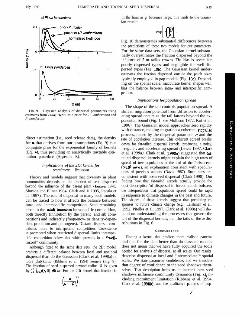
lationship between fall velocities and OL estimates(Greene and Johnson 1989, Okubo and Levin 1989,.Andersen 1991, Clark et al. 1998b) suggests that seedtype provides initi,al information on the dispersal pa-rameter. Therefore, we might exploit confident fits forPinus tigida that result from six years of data in thesouthern Appalachians as a prior for estimating P. lam-bertiana and P. ponderosa. One could argue that thisprior is biased, because P. rigida seeds are smaller (anupward bias in ar), or are released from lower heights(a downward bias in 0~) than are P. lambertiana and P.ponderosa seeds. We do not defend this particularchoice for the prior, as our concern here is simply todemonstrate the approach. (Gelman et al. [ 19951 reviewmethods for checking the fit with data sets simulatedfrom the posterior density.) The normalized likelihood

where S is the new data set, andfla) is a prior densityof a (here, based on P. rigida), is rather broad for P.lambertiana (Fig. 9a) and quite broad for P. ponderosa(Fig. 9b). The breadths of these likelihoods do not re-flect impossibly great dispersal. Rather, the noise in thedata tends to result in relatively flat likelihood surfaces.P. ponderosa densities in clearcuts suggest dispersalmore restricted than that in Fig. 9b (Barrett 1966). Bycontrast, the density for P. rigida (used here as theprior) is concentrated at short distances. The posteriordensities obtained from this Bayesian approach,

JpaIS) =f(a) X NL

probably represent more realistic descriptions for P.lambertiana and P. ponderosa. For example, 95% ofthe density for P. lambertiana decreases from (6.1,76.9) (normalized likelihood) to (4.6; 31.4) (posteriordensity of a).

Moreover, the functional forms used here are es-pecially attractive for fitting the exponentiai family. For

3

.

July 1999 TEMPERATE AND TROPICAL SEED DISPERSAL 1489

a) Pinus lambertiana

0 20 40 60 60 100

a (m)

FIG. 9. Bayesian analysis of dispersal parameters usingestimates from Pinus rigida as a prior for P. lambertiana andP. ponderosa.

direct estimation (i.e., seed release data), the densityfor OL that derives from our assumptions (Eq. 9) is aconjugate prior for the exponential family of kernels(Eq. 4), thus providing an analytically tractable esti-mation procedure (Appendix B).

Implications of the 2Dt kernel forrecruitment limitation

Theory and models suggest that diversity in plantcommunities depends on the fraction of seed dispersedbeyond the influence of the parent plant (Janzen 1970,Shmida and Ellner 1984, Clark and Ji 1995, Pacala etal. 1997). The role of dispersal in many such modelscan be traced to how it affects the balance betweenintra- and interspecific competition. Seed remainingclose to the adultincreases intraspecific competition,both directly (inhibition by the parent ‘and sib com-petition) and indirectly (frequency- or density-depen-dent predation and pathogens). Distant dispersal con-tributes more to interspecific competition. Coexistenceis promoted when restricted dispersal limits interspe-cific competition below that which prevails in a “well-mixed” community.

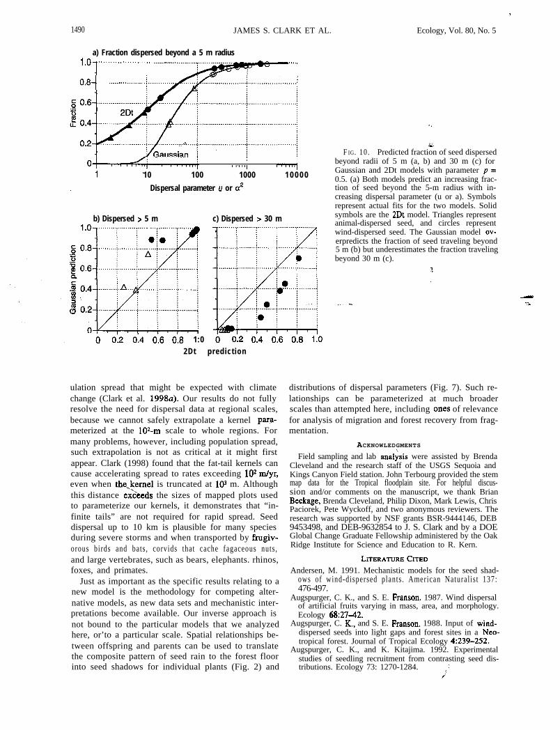
Although fitted to the same data sets, the 2Dt modelpredicts a different balance between local and nonlocaldispersal than do the Gaussian (Clark et al. 1998a) ormore platykurtic (Ribbens et al. 1994) kernels (Fig. 9).The fraction of seed dispersed beyond radius R is givenby j; &,,.&r, 0) d0 dr. For the 2Dt kernel, that fraction is

In the limit as p becomes large, this tends to the Gauss-ian result:

R2exp - -i 01 .

a

Fig. 10 demonstrates substantial differences betweenthe predictions of these two models for our parameters.For the same data sets, the Gaussian kernel substan-tially overestimates the fraction dispersed beyond theinfluence of 5 m radius crowns. The bias is severe forpoorly dispersed types and negligible for well-dis-persed types (Fig. lob). The Gaussian kernel under-estimates the fraction dispersed outside the patch sizestypically employed in gap models (Fig. 10~). Depend-ing on the spatial scale, inaccurate kernel shapes willbias the balance between intra- and interspecific com-petition.

Implications for population spreadThe shape of the tail controls population spread. A

shift in migration potential from diffusion to acceler-ating spread occurs as the tail fattens beyond the ex-ponential bound (Fig. 1; see Mollison 1972, Kot et al.1996). The Gaussian model approaches zero rapidlywith distance, making migration a coherent, stepwiseprocess, paced by the dispersal parameter OL and therate of population increase. This coherent spread breaksdown for fat-tailed dispersal kernels, producing a noisy,irregular, and accelerating spread (Lewis 1997, Clarket al. 1998a). Clark et al. (1998a) suggested that fat-tailed dispersal kernels might explain the high rates ofspread of tree populations at the end of the Pleistocene(>103 m/yr), an explanation consistent with specula-tions of previous authors (Davis 1987). Such rates areconsistent with observed dispersal (Clark 1998). Ourfinding here that fat-tailed kernels actually provide thebest description’of dispersal in forest stands bolstersthe interpretation that population spread could be rapidin response to climate changes in the past and future.The shapes of these kernels suggest that predicting re-sponses to future climate change (e.g., Leishman et al.1992, Pitelka et al. 1997, Clark et al. 1998a) will de-pend on understanding the processes that govern thetail of the dispersal kernels, i.e., the tails of the OL dis-tributions in Fig. 6.

C ONCLUSIONS

Finding a kernel that predicts more realistic patternsand that fits the data better than do classical modelsdoes not mean that we have fully acquired the toolsneeded for analysis of dispersal at all scales. Our resultsdescribe dispersal at local and “intermediate’* spatialscales. We state parameter confidence, and we translatethat degree of confidence to the seed shadows them-selves. That description helps us to interpret how seedshadows influence community dynamics (Fig. 8), in-cluding recruitment limitation (Ribbens et al. 1994,Clark et al. 19986), and the qualitative patterns of pop-

1490 JAMES S. CLARK ET AL.

a) Fraction dispersed beyond a 5 m radius1.0

7. . . . . . . . . . . . . . . . . . . . . . i .___................. . .._.

(4 ..___....._______

:0 8““‘I r 8 1~~~~1

10 100 1000 1 0 0 0 0

Dispersal parameter u or u2

b) Dispersed > 5 m c) Dispersed > 30 m

012 014 0:6 0:8 1:0 012 014 0162Dt prediction

ulation spread that might be expected with climatechange (Clark et al. 1998~). Our results do not fullyresolve the need for dispersal data at regional scales,because we cannot safely extrapolate a kernel para-meterized at the 10*-m scale to whole regions. Formany problems, however, including population spread,such extrapolation is not as critical at it might firstappear. Clark (1998) found that the fat-tail kernels cancause accelerating spread to rates exceeding lo* m/yr,even when the_Femel is truncated at 10” m. Althoughthis distance exseeds the sizes of mapped plots usedto parameterize our kernels, it demonstrates that “in-finite tails” are not required for rapid spread. Seeddispersal up to 10 km is plausible for many speciesduring severe storms and when transported by frugiv-orous birds and bats, corvids that cache fagaceous nuts,and large vertebrates, such as bears, elephants. rhinos,foxes, and primates.

Just as important as the specific results relating to anew model is the methodology for competing alter-native models, as new data sets and mechanistic inter-pretations become available. Our inverse approach isnot bound to the particular models that we analyzedhere, or’to a particular scale. Spatial relationships be-tween offspring and parents can be used to translatethe composite pattern of seed rain to the forest floorinto seed shadows for individual plants (Fig. 2) and

018 110

.

Ecology, Vol. 80, No. 5

:e.F IG. 10. Predicted fraction of seed dispersed

beyond radii of 5 m (a, b) and 30 m (c) forGaussian and 2Dt models with parameter p =0.5. (a) Both models predict an increasing frac-tion of seed beyond the 5-m radius with in-creasing dispersal parameter (u or a). Symbolsrepresent actual fits for the two models. Solidsymbols are the 2Dt model. Triangles representanimal-dispersed seed, and circles representwind-dispersed seed. The Gaussian model ov-erpredicts the fraction of seed traveling beyond5 m (b) but underestimates the fraction travelingbeyond 30 m (c).

*”

--:_.._ “Y”.

distributions of dispersal parameters (Fig. 7). Such re-lationships can be parameterized at much broaderscales than attempted here, including .ones of relevancefor analysis of migration and forest recovery from frag-mentation.

ACKNOWLEDGMENTSField sampling and lab anal&is were assisted by Brenda

Cleveland and the research staff of the USGS Sequoia andKings Canyon Field station. John Terbourg provided the stemmap data for the Tropical floodplain site. For helpful discus-sion and/or comments on the manuscript, we thank BrianBeckage, Brenda Cleveland, Philip Dixon, Mark Lewis, ChrisPaciorek, Pete Wyckoff, and two anonymous reviewers. Theresearch was supported by NSF grants BSR-9444146, DEB9453498, and DEB-9632854 to J. S. Clark and by a DOEGlobal Change Graduate Fellowship administered by the OakRidge Institute for Science and Education to R. Kern.

LITERATURECITEDAndersen, M. 1991. Mechanistic models for the seed shad-

ows of wind-dispersed plants. American Naturalist 137:476-497.

Augspurger, C. K., and S. E. Franson. 1987. Wind dispersalof artificial fruits varying in mass, area, and morphology.Ecology 68:27-42.

Augspurger, C. K.. and S. E. Franson. 1988. Input of wind-dispersed seeds into light gaps and forest sites in a Neo-tropical forest. Journal of Tropical Ecology 4:239-252.

Augspurger, C. K., and K. Kitajima. 1992. Experimentalstudies of seedling recruitment from contrasting seed dis-tributions. Ecology 73: 1270-1284. ;

P

,,July 1999 TEMPERATE AND TROE

Balanda, K. P.; and H. L. MacGillivray. 1988. Kurtosis: acritical review. American Statistician 42: 11 l-l 19.

Barrett, J. W. 1966. A record of ponderosa pine seed flight.U.S. Forest Service Pacific Northwest Forest and RangeExperiment Station PNW-38: l-5.

Bjorkbom, J. C. 1971. Production and germination of paperbirch seed and its dispersal into a forest opening. U.S.Forest Service Research Paper NE-209: l-14.

Carkin, R. E., J. E Franklin, J. Booth, and C. E. Smith. 1978.Seeding habits of upperslope tree species. IV. Seed flightof noble fir and Pacific silver finU.S. Forest Service PacificNorthwest Forest and Range Experiment Station ResearchNote PNW-3121-10.

Chernoff, H. 1954. On the distribution of the likelihood ratio.Annals of Mathematical Statistics 25:573-578.

Clark, J. S. 1998. Why trees migrate so fast: confrontingtheory with dispersal biology and the paleo record. Amer-ican Naturalist 152:204-224.

Clark, J. S., B. Beckage, P Camill, B. Cleveland, J.HilleRisLambers, J. Lichter, J. MacLachlan, J. Mohan, andP Wyckoff. 1999. Interpreting recruitment limitation inforests. American Journal of Botany 86:1-16.

Clark, J. S., C. Fastie, G. Hurt& S. T. Jackson, C. Johnson,G. King, M. Lewis, J. Lynch, S. Pacala, I. C. Prentice, E.W. Schupp, T. Webb III, and P Wyckoff. 1998a. Reid’sParadox of rapid plant migration. Bioscience 48: 13-24.

Clark, J. S., and Y. Ji. 1995. Fecundity and dispersal in plantpopulations: Iimplications for structure and diversity. Amer-ican Naturalist 146:72-l 11.

Clark, J. S., E. Macklin, and L. Wood. 19986. Stages andspatial scales of recruitment limitation in southern Appa-lachian forests. Ecological Monographs 682 13-235.

Curtis, J. D., and M. W. Foiles. 1961. Ponderosa pine seeddissemination into group clearcuttings. Journal of Forestry59:766-767.

Davis, M. B. 1981. Quatemary history and the stability offorest communities. Pages 132-153 in D. C. West, H. H.Shugart, andI D. B. Botkin, editors. Forest succession: con-cepts and application. Springer-Verlag. New York, NewYork, USA.-. 1987. Invasion of forest communities during the

Holocene: beech and hemlock in the Great Lakes region.Pages 373-393 in A. J. Gray, M. J. Crawley, and P. J.Edwards, editors. Colonization, succession, and stability.Blackwell Scientific, Oxford, UK.

Efron, B., and R. J. Tibshirani. 1993. An introduction to thebootstrap. Chapman and Hall, New York, New York, USA.

Fastie, C. L. ‘995. Causes and ecosystem consequences of‘hmultiple pat ways of primary succession at Glacier Bay,

Alaska. EcoIogy 76: 1899-1916.Fowells, H. A.,‘&nd G. H. Schubert. 1956. Seed crops of

forest trees in the pine region of California. USDA Tech-nical Bulletin 1150: l-48.

Gelman, A., J. B. Carlin, H. S. Stern, and D. B. Rubin. 1995.Bayesian data analysis. Chapman and Hall, London, UK.

Geritz, S. A. H,, T. J. de Jong, and P. G. L. Klinkhamer. 1984.The efficacy of dispersal in relation to safe site area andseed production. Oecologia 62:2 19-22 1.

Gladstone, D. E. 1979. Description of a seed-shadow of awind-dispersed tropical tree. Brenesia 16:81-86.

Green, D. S. 1983. The efficacy of dispersal in relation tosafe site denkity. Oecologia 56:356-358.

Greene, D. E, and E. A. Johnson. 1989. A model of winddispersal of winged or plumed seeds. Ecology 70:339-347.

Guevara, S., and J. Laborde. 1993. Monitoring seed dispersalat isolated standing trees in tropical pastures: consequencesfor local species availability. Vegetatio 107/108:319-338.

Holthuijzen, A. M. A., and T. L. Sharik. 1985. The red cedar(Juniperus virginiana L.) seed shadow along a fenceline.American Midland Naturalist 113:200-202.

‘ICAL SEED DISPERSAL 1491

Houle, G. 1992. Spatial relationship betweeen seed and seed-ling abundance and mortality in a deciduous forest of north-eastern North America. Journal of Ecology 80:99-108.

Hughes, J. W., and T. J. Fahey. 1988. Seed dispersal andcolonization in a disturbed northern hardwood forest. Bul-letin of the Torrey Botanical Club 115:89-99.

Hurtt, G. C., and S. W. Pacala. 1995. The consequences ofrecruitment limitation: reconciling chance, history andcompetitive differences between plants. Journal of Theo-retical Biology 176:1-12.

Janzen, D. H. 1970. Herbivores and the number of tree spe-cies in tropical forests. American Naturalist 104:501-528.

Johnson, W. C. 1988. Estimating dispersibility ofAcer, Frax-inus, and Tilia in fragmented landscapes from patterns ofseedling establishment. Landscape Ecology 1: 175-187.

Kot, M., M. A. Lewis, and I? van den Driessche. 1996. Dis-persal data and the spread of invading organisms. Ecology77~2027-2042.

Lamont, B. 1985. Dispersal of the winged fruits of NuyisiaJloribundu (Loranthaceae). Australian Journal of Ecology10: 187-193.

Leishman, M., L. Hughes, K. French, D. Armstrong, and M.Westoby. 1992. Seed and seedling biology in relation tomodelling vegetation dynamics under global climatechange. Australian Journal of Botany 40:599-613.

Levin, S. A. 1976. Population dynamics in heterogeneousenvironments. Annual Review of Ecology and Systematics7:287-3 10.

Levin, S. A., D. Cohen, and A. Hastings. 1984. Dispersal inpatchy environments. Theoretical Population Biology 26:165-191.

Lewis, M. A. 1997. Variability, patchiness and jump dis-persal in the spread of an invading population. Pages 46-69 in D. Tilman and I? Kareiva, editors. Spatial ecology.Princeton University Press, Princeton, New Jersey, USA.

Mair, A. R. 1973. Dissemination of tree seed: Sitka spruce,western hemlock, and Douglas-fir. Scottish Forestry 27:308-3 14.

Mardia, K. V. 1970. Measures of multivariate skewness andkurtosis with application. Biometrika 57~519-530.

Martinez-Ramos, M., and A. Soto-Castro. 1993. Seed rainand advanced regeneration in a tropical rain forest. Vege-tatio 107/10?3:299-318.

Matlack, G. R. 1987. Diaspore size, shape, and fall behaviorin wind-dispersed plant species. American Journal of Bot-any 74:1150-1160.

Mollison, D. 1972. The rate of spatial propagation of simpleepidemics. Proceedings of the Sixth Berkeley Symposiumon Mathematics, Statistics, and Probability 3:579-614.-. 1977. Spatial contact models for ecological and ep-

idemic spread. Journal of the Royal Statistical Society Se-ries B 39:283-326.

Mosteller, F., and J. W. Tukey. 1977. Data analysis and re-gression. Addison-Wesley, Reading, Massachusetts, USA.

Okubo, A., and S. A. Levin. 1989. A theoretical frameworkfor data analysis of wind dispersal of seeds and pollen.Ecology 70:329-338.

Pitelka, L. F., et al. 1997. Plant migration and climate change.American Scientist 85:464-473.

Portnoy, S., and M. E Willson. 1993. Seed dispersal curves:behavior of the tail of the distribution. Evolutionary Bi-ology 7:2544.

Ribbens, E., J. A. Silander. and S. W. Pacala. 1994. Seedlingrecruitment in forests: calibrating models to predict patternsof tree seedling dispersion. Ecology 75: 1794-l 806.

Ritchie, J. C., and G. M. MacDonald. 1986. The patterns ofpost-glacial spread of white spruce. Journal of Biogeog-raphy 13:527-540.

Ruth, R. H., and C. M. Berntsen. 1955. A 4-year record ofSitka spruce and western hemlock seed fallon the Cascade

i

* 4

1492 JAMES S. CLARK ET AL. Ecology, Vol. 80, No. 5 .

Head Experimental Forest. U.S. Forest Service Pacific Shmida, A., and S. Ellner. 1984. Coexistence of plant speciesNorthwest Forest and Range Experiment Station Research with similar niches. Vegetatio 58:29-55.Paper 12:1-13. Stuart, A., and J. K. Ord. 1994. Kendall’s advanced theory

Schupp, E. W. 1990. Annual variation in seedfall, postdis- of statistics. Edward Arnold, New York, New York, USA.persal predation, and recruitment of a neotropical tree. Turchin, I? 1998. Quantitative analysis of movement. Sin-

Ecology 71:504-515. auer, Sunderland, Massachusetts, USA.

Sharpe, D. M., and D. E. Fields. 1982. Integrating the effects Venable, D. L., and J. S. Brown. 1993. The population-

of climate and seed fall velocities on seed dispersal bydynamic functions of seed dispersal. Vegetatio 107/108:3 l-55.

#

wind: a model and application. Ecological Modelling 17: Willson, M. E 1993. Dispersal mode, seed shadows, and297-3 10. colonization patterns. Vegetatio 107/108:261-280.i

,

APPENDIX AMOMENTS AND INDICES DERIVED FROM THEM

To compare dispersal kernels, we require an index thatquantifies shape. Although the term “kurtosis” evokes thisnotion of shape, there is no standard index that enjoys generalacceptance. In this Appendix, we summarize the concept andpropose a simple measure for the case at hand, i.e., a bivariatedispersal kernel with rotational symmetry.

Kurtosis “can be vaguely defined as the location and scale-free movement of probability mass from the shoulders of adistribution to its center and tails” (Balanda and MacGillivray1988: ill), and can be formalized in many ways (see also

M.osteller and Tukey 1977). One class of measures is .basedon moments. Moments are expected values of powers of avariable, which, in some sense, summarize distribution shape.The mean, variance, skewness, and kurtosis involve the firstthrough fourth moments, respectively. The fourth central mo-ment standardized for variance is the most common kurtosismeasure for univariate distributions, but it has an unclearrelationship to shape, and a given value can correspond tomore than one distribution. Moreover, the method used toquantify a shift of mass from the shoulders to peak and tails(scaling) affects the value. (The squared variance is the scal-ing option often used for moment-based measures.) The prob-lems are more complex for bivariate distributions, which in-volve product moments. Despite absence of convention, thereis general agreement that kurtosis measures should be inde-pendent of scale and location. Beyond these criteria, the indexneeds to convey useful information regarding shape.

Here, we describe our moment-based index that is simpleand appropriate for this application (bivariate, rotationallysymmetric distributions in polar coordinates), that is scaleand location-invariant, and that allows comparisons with stan-dard distributions (e.g., Gaussian, exponential). Our moment-based method begins with one for bivariat,e distributions(Mardia 1970) included in a standard reference (Stuart andOrd 1994), but follows with an argument for simplification.We solve for Mardia’s bivariate moments and then demon-strate that the useful information for symmetric distributionsis fully summarized by the simpler (marginal) moments aboutdistance

Shape measures for bivariate kernelsMardia (1970) suggests a measure of kurtosis for the bi-

variate case:

k=!k?!?+ti+?kIGO Pf P2olh2’

(A.11

where CL,,,” is mth and nth central moment over two randomvariables. This formula is typically applied (see examples inMardia 1970 and Stuart and Ord 1994) to distributions definedon the Cartesian plane for random variables (x, y). For the2Dt case, we substitute ra = x2 + y* in Eq. 8 and take momentintegrals to obtain the following complex expression:

x’“y” dy dr[u + x* + yqp+’

u(m+nv*r(y+(qr(p - y)* (A 2) . .=

nr( P) . 1_.,

The resulting kurtosis from the three terms of A.1 is ..,.,..

k(x, y) =3(p - 1) 3(p - 1) 2(6 - 1)-+-+-.p - 2 p - 2 p - 2

(A.3)

For instance, a Gaussian dispersal kernal (obtained in the limitp + “) yields a value of 8 for the Cartesian coordinates (x, y).

The bivariate moments (Eq. A.2) for the rotationally sym-metric kernels that dispersal biologists typically consider areunnecessarily complex and redundant. The complexity of bi-variate moments for the Cartesian locations x and y is un-desirable, because (1) the variable r (distance from the source)is meaningful, whereas location (x, y) is meaningful onlyindirectly; and (2) the solution for r is simple, whereas themoments of (x, y) can be complex (e.g., Stuart and Ord 1994).The first of these two claims is borne out by the fact thatseed dispersal is usually reported as distance from the source,not as Cartesian coordinates. The three terms in Eq. A.3 comefrom the marginal distribution of X, from the marginal dis-tribution of y, and from cross products, respectively. Eachdescribes the same influence of shape parameter p, i.e., @ -I)/@ - 2). We can learn from any one of these terms thatkurtosis is finite so long as p > 2, and that kurtosis declinesto an asymptote as p becomes large. Thus, a measure basedon bivariate moments is unnecessarily complex.

Given that bivariate moments add redundancy, but not in-sight, we consider marginal (univariate) moments of distancer. A simple kuitosis measure for rotationally symmetric dis-tributions is obtained by first integrating the non-informativearc angle out of existence and then solving the moment in-tegral for the marginal density 2nfin(r):

Xrmf (r, 0) d0 dr = 27~ rm+‘f2,,(r) d r

p+,

I II+"p+L a-c (A.4)

I- ulThe substitution v = r2/u yields

f

I

CL, = l&pvm/2

o (1 + Y)p+’ dv* *

Recognizing the integral expression as a beta function,I

t ’ July 1999 TEMPERATE AND TROPICAL. SEED DISPERSAL 1493

1

,!

TB(a, b) =

Z,,+l

0 (1 + zY+bdz = Nmb)

r(a + b)we obtain a simple expression for the mth moment:

Because arguments of the beta function involve integers (mo-ments), it is convenient to recast this result in terms of gammafunctions:

CLm =mumT(m/2)r@ - m/2)

w-9 .Kurtosis is the first term of Eq. A. 1:

(A.5)

0) =!?I 2(P - 1)=-Wt> p;

This compares with that for the exponential family:

k(r) = wdw~)(exponential family) r2(4h) . (A.6b)

Both are scale and location-invariate, involving only the di-mensionless shape parameters p and c, respectively.

One aspect of our foregoing approach deserves mention.Because r is the distance from the mean of a rotationallysymmetric density, Eq. A.4 represents “central” moments,in the sense that they are taken about the mean of the dispersalkernel. They are not centered on the mean of r, because thosemoments would be hard to relate to the density symmetricabout r = 0. Because moments are centered on zero, ratherthan the mean of r, odd moments are not zero; r is the distance

traveled in any direction (we begin the derivation of Eq. A.3by integrating arc angle out of existence). Although the nu-merical values of moments of r (Eq. A.6a) differ from thoseof (x, y) (Eq. A.3), they summarize the same quantity. Forexample, the existence of moments of r implies finite mo-ments in Cartesian space (compare Eqs. A.2 and A.5).

The marginal moments of r (Eq. A.5) and the kurtosismeasure that is based on them (Eq. A.6) capture the essentialfeatures of kernel shape. The simplicity and insight of Eq.A.6 recommends it as a general shape measure for rotationallysymmetric dispersal kernels.

Shape comparisonsEqs. A.6a and A.6b allow comparison of kernel shape for

the two densities considered here. For the 2Dt density, mo-ments smaller than 2p are finite, and kurtosis tends to infinityas p decreases to 2 (Eq. Al.6a). Kurtosis asymptotes at 2 asp becomes large (the Gaussian limit). Potentially large kur-tosis results from the fact that the tail can be extremely fat,precluding convergence of moment integrals. For the expo-nential family, kurtosis is finite, tending to large values as ctends to zero. Values are 2 and 3.33 for Gaussian (c = 2) andexponential (c = l), respectively. Distributions that are morepeaked and fatter tailed than exponential have kurtosis mea-sures B3.33. This value is important in migration studies,because it represents the point at which traveling wave so-lutions yield to accelerating spread (Mollison 1977). Otherkernels in the exponential family used to model dispersalinclude c = 3 (Ribbens et al. 1994) and c = l/2 (Kot et al.1996, Clark 1998), with kurtosis values from Eq. A.6b of1.70 and 9.43, respectively.

APPENDIX BA BAYESIAN LINKTO DIRECT KERNEL ESTIMATION

The likelihood of observine n seeds. each of which travelsThe inverse approach is applied to spatial patterns of seedrain having a complex, distributed source. The model devel-oped here can also be applied to the direct approach, in whichseeds are released and settling distances r are recorded (e.g.,Augspurger and Franson 1987, Matlack 1987). We demon-strate the connection between variability in a and kernelshape, as represented by our densitiesf(a) andf(r) a), in aBayesian context. To simplify our likelihood, we assume thatall released seed is recovered. This assumption allows us towrite a likelihood based directly on the density of r, as op-posed to a binomial (with some probability of recovery) with-in whichf(r) is embedded.

”distance r,, is given by

f(rl4 = fi f(r,la)

C”

= 2wa~ P(2k) exp Iand the marginal density is

03.2)

f(r) =f9g-(p,)

2~p~r~(uc)r(p)u9The ZDt%iodel involves a conjugate prior

Assume that seed is dispersed according to an exponentialkernel family. The sampling distribution is given by Eq. 4.Assuming that the variable

A=:

is gamma distributed, we use the previous approach to obtainthe prior density of a: m .

f(a) cuf;= - e x p -2,aq+lr(p) I I

(B:l)

where u0 is our prior estimate of u. Integrating Eq. 4 overvariability in a gives the marginal density for this exponentialfamily:

x

f(r) = f(alf(rla) da =cup

2nB(2k, p)(u + rcYwhere P = 2lc 4 p.

where U,, = uO + XL, r; and Pa = 2n/c + p. The posteriordensity is also inverse x2:

CUE

f (alr) = acp.+~r(p,)exP 03.3)

which has the same form as Eq. B. 1, thus showing Eq. B.lto be a conjugate prior for the exponential family f (r I a). Theprior estimate of us has a contribution equivalent to l/n. It isfurther evident from Eq. B.3 that the posterior becomes in-creasingly peaked with increasing sample size, and the kernelf(r) tends to the exponential family.

ExampleA simple data set demonstrates application of the direct

method. Dispersal distances of Fraxinus americana seedswere recorded from the point of release at a height of 4 mon a calm day. Wind speeds during the experiment rangedfrom 0 to 0.7 m/s and averaged 0.2 m/s. Seeds were releasedthree times in groups of five to produce the vector of radii

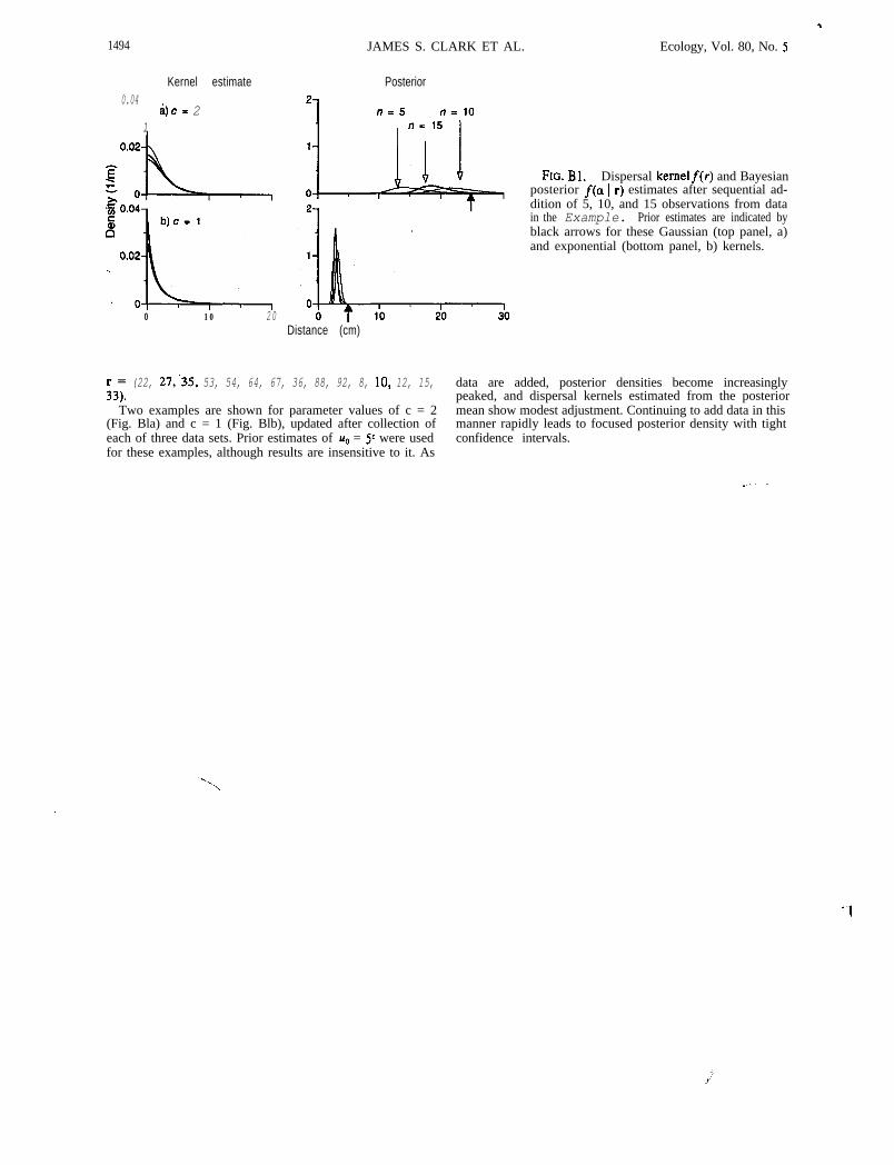
1494

Kernel estimate0.04

1i)c= 2

JAMES S. CLARK ET AL.

Posterior

Ecology, Vol. 80, No. 5

0 10 20Distance (cm)

FIG. Bl. Dispersal kernelf and Bayesianposterior f(a 1 r) estimates after sequential ad-dition of 5, 10, and 15 observations from datain the Example. Prior estimates are indicated byblack arrows for these Gaussian (top panel, a)and exponential (bottom panel, b) kernels.

& (22, 27;35, 53, 54, 64, 67, 36, 88, 92, 8, 10, 12, 15, data are added, posterior densities become increasinglypeaked, and dispersal kernels estimated from the posterior

Two examples are shown for parameter values of c = 2 mean show modest adjustment. Continuing to add data in this(Fig. Bla) and c = 1 (Fig. Blb), updated after collection of manner rapidly leads to focused posterior density with tighteach of three data sets. Prior estimates of u,, = 5’ were used confidence intervals.for these examples, although results are insensitive to it. As