NOAA Technical Report NOS CO-OPS 086

noaa National Oceanic and Atmospheric Administration

U.S. DEPARTMENT OF COMMERCE National Ocean Service Center for Operational Oceanographic Products and Services

PATTERNS AND PROJECTIONS OF HIGH TIDE FLOODING ALONG THE U.S. COASTLINE USING A COMMON IMPACT THRESHOLD

Silver Spring, Maryland February 2018

Photo: New York City Harbor

Center for Operational Oceanographic Products and Services National Ocean Service

National Oceanic and Atmospheric Administration U.S. Department of Commerce

The National Ocean Service (NOS) Center for Operational Oceanographic Products and Services (CO-OPS) provides the National infrastructure, science, and technical expertise to collect and distribute observations and predictions of water levels and currents to ensure safe, efficient and environmentally sound maritime commerce. The Center provides the set of water level and tidal current products required to support NOS’ Strategic Plan mission requirements, and to assist in providing operational oceanographic data/products required by NOAA’s other Strategic Plan themes. For example, CO-OPS provides data and products required by the National Weather Service to meet its flood and tsunami warning responsibilities. The Center manages the National Water Level Observation Network (NWLON), a national network of Physical Oceanographic Real-Time Systems (PORTS®) in major U. S. harbors, and the National Current Observation Program consisting of current surveys in near shore and coastal areas utilizing bottom mounted platforms, subsurface buoys, and horizontal sensors. The Center: establishes standards for the collection and processing of water level and current data; collects and documents user requirements, which serve as the foundation for all resulting program activities; designs new and/or improved oceanographic observing systems; designs software to improve CO-OPS’ data processing capabilities; maintains and operates oceanographic observing systems; performs operational data analysis/quality control; and produces/disseminates oceanographic products.

NOAA Technical Report NOS CO-OPS 086

U.S. DEPARTMENT OF COMMERCE Wilbur Ross, Secretary National Oceanic and Atmospheric Administration RDML Tim Gallaudet, Ph.D., USN Ret. Assistant Secretary of Commerce for Oceans and Atmosphere and Acting Under Secretary of Commerce for Oceans and Atmosphere National Ocean Service Dr. Russell Callender, Assistant Administrator Center for Operational Oceanographic Products and Services Richard Edwing, Director

Patterns and Projections of High Tide Flooding Along the U.S. Coastline Using a Common Impact Threshold

William V. Sweet National Oceanic and Atmospheric Administration, National Ocean Service, Center for Operational Oceanographic Products and Services, Silver Spring, MD, USA

Greg Dusek National Oceanic and Atmospheric Administration, National Ocean Service, Center for Operational Oceanographic Products and Services, Silver Spring, MD, USA

Jayantha Obeysekera South Florida Water Management District, West Palm Beach, FL

John J. Marra National Oceanic and Atmospheric Administration, National Environmental Satellite, Data, and Information Services, National Centers for Environmental Information, Honolulu, HI, USA

February 2018

NOTICE

Mention of a commercial company or product does not constitute an endorsement by NOAA. Use of information from this publication for publicity or advertising purposes concerning proprietary products or the tests of such products is not authorized.

iii

TABLE OF CONTENTS TABLE OF CONTENTS ......................................................................................................................................... III

LIST OF FIGURES .................................................................................................................................................. IV

LIST OF TABLES .................................................................................................................................................... VI

EXECUTIVE SUMMARY ...................................................................................................................................... VII

1.0 INTRODUCTION ......................................................................................................................................... 1

2.0 DEFINING A CONSISTENT COASTAL FLOOD ELEVATION THRESHOLD .................................. 7

3.0 HISTORICAL PATTERNS OF HIGH TIDE FLOODING ................................................................... 13 3.1 TRENDS IN HIGH TIDE FLOODING ............................................................................................................................... 13 3.2 YEAR-TO-YEAR VARIABILITY IN HIGH TIDE FLOODING DUE TO ENSO ............................................................... 17 3.3 SEASONAL CYCLES IN HIGH TIDE FLOODING ............................................................................................................ 20

4.0 FUTURE PROJECTIONS OF HIGH TIDE FLOODING ...................................................................... 23

5.0 SUMMARY REMARKS ............................................................................................................................ 31

ACKNOWLEDGEMENTS ..................................................................................................................................... 35

REFERENCES ......................................................................................................................................................... 35

APPENDIX 1 .......................................................................................................................................................... 41

APPENDIX 2 .......................................................................................................................................................... 44

iv

LIST OF FIGURES Figure 1. a) Long-term (>30 years record) RSL trends around the U.S. coastline measured

and/or computed by NOAA (Zervas, 2009), b) multi-year empirical (smoothed) distributions for daily highest water levels in Norfolk, Virginia for the 1960s and 2010s, showing extent that local RSL rise has increased the flood probability relative to impact thresholds defined locally by the NOAA NWS for minor (~0.5 m: nuisance level), moderate (~0.8 m) and major (~1.2 m: local level of Hurricane Sandy in 2012) impacts, relative to mean higher high water (MHHW) tidal datum and in c) are annual flood frequencies (based upon 5-year averages) in Norfolk for high tide floods with minor impacts shown as accelerating by the quadratic trend fit (goodness of fit [R2]=0.84). Figure from Sweet et al. (2017a). ..................................................................................... 3

Figure 2. a) Long-term tide gauges with official NOAA flood thresholds for minor (high tide) flooding with exposed topography (red) mapped by the NOAA SLR Viewer and b) the annual summation of days with high tide flooding at locations shown in a) during 2016 as monitored by NOAA (Sweet et al., 2017b). ................................................................. 4

Figure 3. Scatter plot of NOAA tide gauge locations with official NOAA coastal flood thresholds (y-axis) shown relative to MLLW tidal datum for minor, moderate and major impacts and the diurnal tide range (GT). There are 66 tide gauges with minor (high tide), 48 with moderate and 46 with major flood thresholds. Locations in the continental U.S. are shown as circles, whereas those in Alaska are designated by triangles. No official NOAA coastal flood thresholds exist for island states or territories. Linear regression fits (black line and boxed equation) and the 90% confidence interval (5% and 95% as red dashed lines) are also shown. Derived thresholds are obtained by solving the regression equations for a particular location. For example, y (the minor derived flood threshold for a location) = 1.04 * x (the local GT tidal datum) + 0.50 m. All NOAA official flood thresholds were obtained in July 2017. ...................................................... 8

Figure 4. The official NOAA and derived elevation thresholds for high tide/minor (a, b), moderate (c, d) and major (e, f) flooding. Note that the legend scales increase by 0.3 m (about 1 foot) between minor, moderate and major flooding threshold elevations. Black dots denote locations without an official NOAA flood threshold. ................................. 10

Figure 5. Recurrence intervals for the NOAA and derived elevation thresholds for high tide/minor (a, b), moderate (c, d) and major (e, f) flooding adjusted to year 2000 sea levels. Black dots denote locations without a NOAA flood threshold. .......................... 12

Figure 6. Annual number of high tide floods (days per year) at NOAA tide gauge locations. A year is defined in terms of a meteorological year (May–April). Note: White squares indicate no data or that hourly data was less than 80% complete within a year. ........... 14

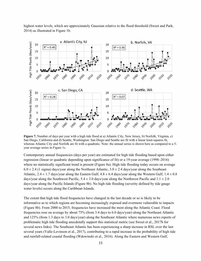
Figure 7. Number of days per year with a high tide flood at a) Atlantic City, New Jersey, b) Norfolk, Virginia, c) San Diego, California and d) Seattle, Washington. San Diego and Seattle are fit with a linear least-squares fit, whereas Atlantic City and Norfolk are fit with a quadratic. Note: the annual series is shown here as compared to a 5-year average series in Figure 1c. .......................................................................................................... 15

Figure 8. a) Number of days in 2015 with a high tide flood derived by trend (linear or quadratic fits above the 90% significance level) or 19-year average (1998–2016) where no significant trend exists. Black dots denote locations with no floods over the 1998–2016 period and b) is the percent change since 2000 based upon trend fits also used in a). Black dots denote locations as in a) or where no significant trend exists. ..................... 16

v

Figure 9. a) Variance of 1998–2016 daily highest water levels, b) the ratio between variances of daily highest predicted tidal component of water level to observed water levels and examples at c) Norfolk, Virginia and d) San Diego, California showing daily highest waters (red), contribution from daily highest predicted tide (blue); both are shown relative to their minor derived flood threshold (green), and the ratio is listed in parentheses. .................................................................................................................... 17

Figure 10. Parametric probability distribution (normal) fit for 3 years characterized by stronger El Niño, stronger La Niña and ENSO-neutral conditions. In parentheses are the mean and standard deviation (or square of the variance) of the distributions shown in the figures. Water levels have been detrended to enable multi-year comparisons. Not shown are the 95% confidence intervals for the distribution parameters which suggest a significant change of conditions during El Niño along both of these (and other) West and East Coast locations. ................................................................................................ 18

Figure 11. Trends in annual frequencies of high tide flooding (black line) are fit to observed annual flood frequencies (black line-dots) over the 1950–2016 period (or beginning of record) as shown in Figure 6. Predictions of high tide flooding based on both trend and annual averaged ENSO effects (ONI) are also shown (red line-dots) for a) Atlantic City, b) Norfolk, c) San Diego and D) Seattle. ....................................................................... 19

Figure 12. a) Characterization of regression trend estimates of increasing decadal annual high tide flood frequencies: accelerating (quadratic) or linear increasing or no trend (black dot) and b) locations whose high tide flood frequencies change on an interannual basis due to phases of ENSO as illustrated in Figure 11. Specifically, in b) are predictions for days in 2015 (May 2015–April 2016) with high tide flooding considering the predicted strength of El Niño (based upon ONI) relative to values based on the trend-derived or 19-year average value as shown in Figure 8a. Kwajalein Island (blue dot) in Figure 12b is opposite the other locations—flood frequencies drop during El Niño and rise during La Niña. .......................................................................................................................... 20

Figure 13. a) Percentage of high tide floods caused solely by tidal forcing over latest 19-year tidal epoch (1998–2016), with black dots designating locations with no high tide floods caused by tides alone or for locations with no high tide flooding during this period. For instance, 20% of San Diego’s high tide floods are caused by tides alone, whereas in New York City, the tide alone is insufficient to cause flooding, b) and c) high tide flooding in San Diego and New York City (NYC) since 1980 distributed by month and d) is the percentage of high tide flood days experienced over 1998–2016 by month at 99 NOAA tide gauges. ........................................................................................................ 21

Figure 14. Projected annual frequencies of high tide flooding in response to scenarios of global sea level rise (Sweet et al., 2017) estimated at NOAA tide gauges in a) New York City (The Battery), b) Miami (Virginia Key), Florida and c) San Francisco, California considering observed patterns (combined tidal and nontidal water level components) and d), e) and f) at the same locations but assuming predicted tide forcing only. Derived high tide flood levels are 0.56 m, 0.53 m and 0.57 m, respectively. .............................. 24

Figure 15. Projected annual frequencies of high tide flooding by 2050 (average over the 2041–2050 period) in response to the a) Intermediate Low and c) Intermediate Scenarios of global sea level rise (Sweet et al., 2017a) estimated at 99 NOAA tide gauges based upon historical patterns and percentage of floods caused by tide forcing alone in b) and d), respectively. Black dots in b) denote locations where tide alone does not exceed the minor derived flood threshold. ....................................................................................... 25

vi

Figure 16. As in Figure 15, but for projected annual frequencies of high tide flooding by 2100 (average over the 2091–2100 period). ............................................................................ 26

Figure 17. a) Empirical probability densities for daily highest water levels over 1998-2016 at Miami, Florida and New York City showing differences in variance (color-coded in box and in units of m2), b) locations with linear trends (significant above 90% level) in variance computed for daily high water levels per year and relative comparison between annual mean sea level and standard deviation (variance0.5) and fitted linear trends of daily highest levels per year at c) Bergen Point, New York and d) Beaufort, North Carolina where significant trends in annual variance occur. .......................................... 27

Figure 18. a) Daily exceedance probabilities (1-cumulative distribution) within a year for New York City (The Battery), Norfolk (Sewells Point), Virginia and Miami (Virginia Key), Florida based upon daily highest water levels over the 1998–2016 period with their average high tide/minor, moderate and major flood thresholds labeled. The decade when MHHW reaches the b) high tide/minor threshold, c) moderate threshold and d) major threshold levels for coastal flooding for local RSL projections under the Intermediate Scenario developed by the Federal Interagency Sea Level Rise and Coastal Flood Hazard Task Force (Sweet et al., 2017a). ............................................................ 29

LIST OF TABLES Table 1. Processes affecting water levels and their temporal scales. Tide gauges, whose samples

are composed of multi-minutes averages, generally do not include wave contributions or their effects. Modification of Table 1 of Sweet et al. (2017a). ........................................ 2

vii

EXECUTIVE SUMMARY

For forecasting purposes to ensure public safety, NOAA has established three coastal flood severity thresholds. The thresholds are based upon water level heights empirically calibrated to NOAA tide gauge measurements from years of impact monitoring by its Weather Forecast Offices (WFO) and emergency managers. When minor (more disruptive than damaging), moderate (damaging) or major (destructive) coastal flooding is anticipated (not associated with tropical storms), NOAA issues either a flood advisory (for minor) or warning (for moderate or major). Less than half of NOAA tide gauges located along the U.S. coastline have such ‘official’ NOAA flood thresholds, and where they exist, the heights can vary substantially (e.g., 0.3–0.6 meter within minor category). They differ due to the extent of infrastructure vulnerabilities, which vary by topography and relief, land-cover types or existing flood defenses.

We find that all official NOAA coastal flood thresholds share a common pattern based upon the local tide range (possibly in response to systematic development ordinances). Minor, moderate and major coastal flooding typically begin about 0.5 m, 0.8 m and 1.2 m above a height slightly higher than the multi-year average of the daily highest water levels measured by NOAA tide gauges. Based upon this statistical (regression-based) relationship, a ‘derived’ set of flood threshold proxies for minor, moderate or major impacts are permissible for almost any location along the U.S. coastline.

The intent of this report is not to supplant knowledge about local flood risk. Rather, the intention is to provide an objective and nationally consistent set of impact thresholds for minor/moderate/major coastal flooding. Such definitions are currently lacking, which limits the ability to deliver new products as well as the effectiveness of existing coastal flood products. Coastal communities along all U.S. coastlines need consistent guidance about flooding, which is 1) forecasted in the near future (e.g., severity/depth of 4-day predictions of storm surge heights ‘above ground level’), 2) likely in the coming season or year (e.g., probabilistic outlooks) or 3) possible over the longer term (e.g., decadal to end-of-century scenarios). Our primary emphasis is to use the derived threshold for minor flooding, which we refer to as ‘high tide’ flooding (also known as ‘nuisance’, ‘sunny day’ and ‘recurrent tidal’ flooding), to assess nationally how exposure—and potential vulnerability—to high tide flooding has and will continue to change with changing sea levels.

High tide flooding today mostly affects low-lying and exposed assets or infrastructure, such as roads, harbors, beaches, public storm-, waste- and fresh-water systems and private and commercial properties. Due to rising relative sea level (RSL), more and more cities are becoming increasingly exposed and evermore vulnerable to high tide flooding, which is rapidly increasing in frequency, depth and extent along many U.S. coastlines. Today, high tide flooding is likely more disruptive (a nuisance) than damaging. The cumulative effects, however, are becoming a serious problem in several locations including many with strategic importance to national security such as Norfolk, Virginia, San Diego, California and Kwajalein Island in the U.S. Marshall Islands.

Over the last several decades, annual frequencies of high tide flooding are found to be linearly increasing in 31 locations (out of 99 tide gauges examined outside Alaska) mostly along the coasts of the Northeast/Southeast Atlantic and the Eastern/Western Gulf of Mexico, and to a lesser extent, along the Northwest and Southwest Pacific coasts. Annual frequencies are accelerating (nonlinearly increasing) in 30 locations mostly along the Northeast and Southeast Atlantic Coasts. Currently, high tide flood

viii

frequencies are increasing at the highest overall rates (and likely becoming most problematic) along the coasts of the Southeast Atlantic and to a lesser extent along the Northeast Atlantic and the Western Gulf. Between 2000 and 2015, annual frequencies increased (median values) by about 125% (from 1.3 days to 3.0 days/year) along the Southeast Atlantic, by 75% (from 3.4 days to 6.0 days/year) along the Northeast Atlantic and by 75% (from 1.4 days to 2.5 days/year) along the Western Gulf.

High tide flooding is currently less problematic along the coasts of the Northwest and Southwest Pacific and the U.S. Pacific (Kwajalein Island being an exception) and Caribbean Islands for two main reasons: 1) the local height of the high tide flood threshold is above the reach of all or most of the annual highest water levels due to a combination of generally calmer weather conditions or bathymetric constraints that limit storm surge potential and 2) regionally RSL rise rates have been relatively low over the last several decades. In these locations, however, large waves (swells) and their high-frequency dynamical effects, which are generally not inherent to NOAA tide gauge measurements, can override high tides and cause dune overwash, coastal erosion and flooding.

High tide flooding regionally occurs more often in certain seasons and during certain years, which is important for awareness and preparedness purposes. The seasonality in flood frequency occurs in response to a spatially varying mixture of rhythmic astronomical tides (‘tidal forcing’), repetitive seasonal mean sea level cycles and less-predictable episodic changes in wind and ocean currents that are nontidal in origin. Frequencies are relatively high during September–April along the Northeast Atlantic Coast and generally peak in October–November. Along the Southeast Atlantic and Gulf Coasts, frequencies are highest during September–November with a secondary peak in June–July. Along both the Northwest and Southwest Pacific, frequencies are highest during November–February with a secondary peak in June–July along the Southwest Pacific.

High tide flood frequencies vary year-to-year due to large-scale changes in weather and ocean circulation patterns, such as during the El Niño Southern Oscillation (ENSO). During the El Niño phase, high tide flood frequencies are amplified at 49 (about half of examined) locations along the U.S. West and East Coasts beyond underlying RSL rise-forced trend increases. This predictable ENSO response may better inform annual budgeting in some flood-prone locations for emergency mobilizations and proactive responses. For example, during 2015, high tide flood frequencies were predicted to be 70% and 170% higher than normally would be expected (e.g., above trend values) along the East and West Coasts, respectively, based upon the predicted El Niño strength about a year in advance. Subsequent monitoring the following year verified that a strong El Niño formed, and flood frequencies occurred at or above the trend/ENSO predicted values at many locations.

With continued RSL rise, high tide flood frequencies will continue to rapidly increase and more so simply from tidal forcing, which today is very rare. We assess future changes locally projected under a subset of the global rise scenarios of the U.S. Federal Interagency Sea Level Rise and Coastal Flood Hazard Task Force, specifically the Intermediate Low (0.5 m global rise by 2100) and Intermediate (1.0 m global rise) scenarios. Under these two scenarios, by 2050, annual high tide flood frequencies along the Western Gulf (80 and 185 days/year, respectively) and Northeast Atlantic (45 and 130 days/year) are higher largely because RSL rise is projected to be higher. Along coasts of the Southeast Atlantic (25 and 85 days/year), the Eastern Gulf (25 and 80 days/year), the Southwest (15 and 35 days/year) and Northwest Pacific (15 and 30 days/year), the Pacific (5 and 45 days/year) and Caribbean Islands (0 and 5 days/year), high tide flooding occurs less often because RSL rise projections are lower or weather conditions are typically

ix

calmer; however, the rate of increase in annual flood frequencies will eventually increase at very rapid rates. On average across all regions, high tide flooding by 2050 will occur about 35% and 60% of the times solely from tidal forcing under the Intermediate Low and Intermediate Scenarios, respectively.

By 2100, high tide flooding will occur ‘every other day’ (182 days/year) or more often under the Intermediate Low Scenario within the Northeast and Southeast Atlantic, the Eastern and Western Gulf, and the Pacific Islands with tidal forcing causing all (100%) of the floods except within the Eastern Gulf (80% caused by tides). By definition, ‘every other day’ high tide flooding would bring to fruition the saying championed by NOAA’s (late) Margaret Davidson: “Today’s flood will become tomorrow’s high tide.” Under the Intermediate Scenario, high tide flooding will become ‘daily’ flooding (365 days/year with high tide flooding) within nearly all regions with tide forcing alone, causing 100% of flooding.

Lastly, these results illustrate how close U.S. coastal cities are to a tipping point with respect to flood frequency, as only 0.3m to 0.7 m separates infrequent damaging-to-destructive flooding from a regime of high tide flooding—or minor floods from moderate and major floods. This suggests a particular interpretation for ‘freeboard’ and other engineering adaptive methods as the desired level of protection in terms of flood type, in both the present and future. This recognition may in turn facilitate a more systematic implementation of freeboard guidelines nationally.

1

1.0 INTRODUCTION

Tide gauges of the National Oceanic and Atmospheric Administration (NOAA) National Ocean Service (NOS) have been measuring water levels along U.S coastlines for more than a century1. Their real-time data resolve a range of motion and variability associated with a variety of processes (Table 1). Their observations resolve the rhythmic nature of the astronomical tides (‘tidal forcing’), seasonal changes in local mean sea level and episodic, often-damaging, storm surges (Table 1); both the tidal and seasonal cycles are included in NOAA tide predictions2 and provide highly accurate (non-storm-related) forecasts about water levels at any time and place along the U.S. coastline. As such, NOAA’s national tide gauge network is key to supporting maritime safety and commerce, defining the country’s maritime-economic boundaries and preparing for emergencies during coastal storms. Tide gauge data also reveal that relative sea levels (RSL) have been increasing by about 2–5 mm/year (0.8–2.0 inches/decade) or more over the last several decades around much of the continental U.S., Hawai'i and island territories (Figure 1a)3 due to a variety of factors affecting regional sea surface height and land elevations (Table 1: Zervas, 2009; Church and White, 2011; Hay et al., 2015; Kopp et al., 2015; Sweet et al., 2017a, Hsu and Velicogna, 2017). As the vertical gap between coastal infrastructure and the ocean decreases, the risk of flooding increases (Figure 1b). Decades ago, powerful storms typically caused coastal flooding, but due to RSL rise, rather common wind events and seasonally high tides now more often cause the ocean to spill into communities (Sweet et al., 2014). Other impacts include infiltration and degradation of stormwater (Obeysekera et al., 2011) and wastewater (Flood and Cahoon, 2011) systems and saltwater intrusion that raises coastal groundwater tables (Sukop et al., 2018. Flood severity becomes further compounded if large swells (Serafin et al., 2017), heavy rainfall (Wahl et al., 2015) or high river flows occur (Moftakhari et al., 2017a) concurrently, the effects of which, however, are not generally measured by tide gauges (Table 1).

1 https://tidesandcurrents.noaa.gov 2 https://tidesandcurrents.noaa.gov/tide_predictions.html 3 https://tidesandcurrents.noaa.gov/sltrends/sltrends.html

2

Table 1. Processes affecting water levels and their temporal scales. Tide gauges, whose samples are composed of multi-minutes averages, generally do not include wave contributions or their effects. Modification of Table 1 of Sweet et al. (2017a).

Over the last several decades, a rapid—accelerating in many locations—change in the annual frequencies of tidal flooding has been documented at NOAA tide gauges along the U.S. coastline (Figure 1c). The cause for the increase is RSL rise (Ezer and Atkinson, 2014; Sweet et al., 2014; Sweet et al., 2017a, c), with annual flood frequencies in several U.S. East and West Coast cities further influenced on a year-to-year basis by the El Niño Southern Oscillation (ENSO) (Sweet and Park, 2014). In many coastal cities, ‘minor’ tidal flooding now occurs several times a year and is often referred to as ‘recurrent’, ‘sunny-day’, ‘shallow coastal’ or ‘nuisance’ flooding. More-severe (deeper, more widespread and typically storm-driven) ‘moderate’ and ‘major’ flooding has become and will continue to become more probable (e.g., Tebaldi et al., 2012; Salas and Obeysekera, 2014; Sweet et al., 2013, 2017a; Kopp et al., 2014; Buchanan et al., 2016, 2017; Vitousek et al., 2017). Flood heights are operationally forecasted by NOAA’s National Weather Service (NWS) Weather Forecast Offices (WFO). If flooding above the minor, moderate or major impact categories (not associated with tropical cyclones) is likely or imminent, NOAA issues guidance to inform the public of potential risks and assist local emergency managers (NOAA, 2017)4.

4 See http://water.weather.gov/ahps

3

Figure 1. a) Long-term (>30 years record) RSL trends around the U.S. coastline measured and/or computed by NOAA (Zervas, 2009), b) multi-year empirical (smoothed) distributions for daily highest water levels in Norfolk, Virginia for the 1960s and 2010s, showing extent that local RSL rise has increased the flood probability relative to impact thresholds defined locally by the NOAA NWS for minor (~0.5 m: nuisance level), moderate (~0.8 m) and major (~1.2 m: local level of Hurricane Sandy in 2012) impacts, relative to mean higher high water (MHHW) tidal datum and in c) are annual flood frequencies (based upon 5-year averages) in Norfolk for high tide floods with minor impacts shown as accelerating by the quadratic trend fit (goodness of fit [R2]=0.84). Figure from Sweet et al. (2017a).

The extent and severity of impacts under the three flood categories have been empirically calibrated to some—but not all—NOAA tide gauge levels through years of impact monitoring by NOAA NWS WFOs and local city emergency managers. Periodically, the thresholds are adjusted to reflect a change in infrastructure vulnerabilities or for communication purposes (e.g., minimize ‘warning fatigue’). NOAA coastal flood elevation thresholds (henceforth referred to as ‘official NOAA’ thresholds) vary by location as shown for a subset of tide gauges recently analyzed by Sweet et al. (2017b) (Figure 2). According to WFOs around the U.S., differences reflect the location and extent of exposed infrastructure in a given region of emphasis (e.g., a particular roadway or an entire city section), which are a function of topography, land use and existing flood mitigation strategies (e.g., hurricane floodwalls). For instance, in Wilmington, North Carolina, the official NOAA minor flood threshold is 0.25 m above the mean higher high water (MHHW) tidal datum, whereas it is about 0.5 m and 0.75 m above MHHW in Norfolk, Virginia and Galveston, Texas, respectively. When minor (henceforth referred to as ‘high tide’) flooding is likely, NOAA typically issues a coastal flood ‘advisory’, whereas when more-severe moderate and major flooding is imminent—usually due to localized storm effects—a coastal flood ‘warning’ of serious risks to life and property is issued (NOAA, 2017).

As sea levels continue to rise, not only will the frequency, depth, and extent of coastal flooding continue to rapidly increase, but they will do so largely in response to repetitive astronomical and seasonal forcing alone (Ray and Foster, 2016). The U.S. military recognizes that changes in RSL rise-related flooding pose a serious risk to their efforts and have developed tools for their engineers to estimate future sea levels and

4

flood risk (Moritz et al., 2015; Hall et al., 2016)5. It is important for planning purposes that U.S. coastal cities become better informed about the extent that high tide flooding is increasing and will likely increase in the coming decades. Of concern is that the cumulative flood toll and response costs of many lesser floods will overtake that of major, but much rarer, events (Moftakhari et al., 2017b). This concern arises because annual flood frequencies of lesser extremes are projected to (or continue to) accelerate at a faster pace (Sweet and Park, 2014; Dahl et al., 2017; Moftakhari et al., 2015; Sweet et al., 2017a) as has been observed over the last several decades at a set of actively monitored U.S. tide gauge locations (Figure 2b).

Figure 2. a) Long-term tide gauges with official NOAA flood thresholds for minor (high tide) flooding with exposed topography (red) mapped by the NOAA SLR Viewer6 and b) the annual summation of days with high tide flooding at locations shown in a) during 2016 as monitored by NOAA (Sweet et al., 2017b).

The intent of this report is not to supplant knowledge about local flood risk. Rather, the goal is to use the set of NOAA flood heights—where they exist—to derive a nationally consistent definition of coastal flooding and impacts used in quantifying and communicating risk7. Such a set of spatially consistent coastal flood thresholds (henceforth referred to as ‘derived’ flood thresholds) is currently lacking, which limits the ability to develop new products or the effectiveness of existing products that provide national coverage. A few examples include describing flood severity associated with an anticipated storm surge or coastal flood (e.g., relative to ‘ground level’), seasonal/annual monitoring and predictions of flood frequency changes (Sweet and Marra, 2015, 2016; Sweet et al., 2017b; Widlansky et al., 2017) and multi-decadal vulnerability assessments considering current and future possible sea level rise (Hall et al., 2016; Sweet et al., 2017a, c).

After presenting the derived set of flood elevation thresholds, the remainder of the report utilizes these derived thresholds for high-tide flooding (unless otherwise noted) to examine flood-frequency changes

5 See also http://www.corpsclimate.us/ccaceslcurves.cfm 6 See https://coast.noaa.gov/slr/ 7 See http://www.weather.gov/images/akq/hydro/Coastal_Flooding/CoastalFloodingThresholds.png

5

and patterns at 99 NOAA tide gauge locations with >20 years of hourly data. In many instances the results are presented by geographic region (listed in Appendix 1), which are defined as tide gauge locations within the 1) Northeast Atlantic (Maine to Virginia), Southeast Atlantic (North Carolina to Florida), Caribbean Islands (Virgin Islands and Puerto Rico), Eastern Gulf of Mexico (Florida to Mississippi), Western Gulf (Louisiana to Texas), Southwest Pacific (San Diego to Arena Cove, California), Northwest Pacific (Humboldt Bay, California to Washington State) and the Pacific Islands (Hawai’i, Guam, American Samoa, Kwajalein, Midway and Wake Islands).

Flood frequency changes are documented in terms of past patterns, current conditions and future projections, specifically detailing:

• current trends to raise awareness of where and to what depth and possible topographic extent flood risks are rising and threatening coasts now due to RSL rise (Ezer and Atkinson, 2014; Sweet et al., 2014; Sweet and Park, 2014; Karegar et al., 2017);

• seasonal cycles to support preparedness efforts by identifying when during the year flooding is most typical;

• year-to-year changes from ENSO to support experimental ‘next-year’ predictions in response to forecasted ENSO phases and historical trend continuation (Sweet and Marra, 2015, 2016; Sweet et al., 2017b), which will become increasingly important for municipal budgeting purposes (mobilization costs for closing streets, installing pumps, sandbags, in-flow stormwater preventers, etc.);

• projections in response to future sea level rise scenarios (Sweet et al., 2017a) in terms of both historical water level observations (tides + nontidal ‘weather’) and predictions based upon tidal forcing alone to assist long-term planning concerned with flood risk reduction and freshwater management (Sweet and Park, 2014; Moftakhari et al., 2015; Hughes and White, 2016; Ray and Foster, 2016; Dahl et al., 2017; Habel et al., 2017; Sweet et al., 2017a).

6

7

2.0 DEFINING A CONSISTENT COASTAL FLOOD ELEVATION THRESHOLD

Most, but not all, of the official NOAA coastal flood thresholds established locally by emergency managers and NOAA WFOs are shown in the Advanced Hydrologic Prediction System8. This system warns of possible, predicted or ongoing hydrologic threats across the U.S., though it is primarily focused on inland flooding and tracks a vast array of national river gauges. It also tracks conditions along the coast and currently includes (subject to change) about 75 flood-hazard definitions for minor (i.e., high tide) and 50 for moderate and major coastal flooding that reference levels on NOAA tide gauges.

Previous efforts have attempted to broadly describe the official NOAA coastal flood thresholds based upon statistical analysis of flood frequencies (e.g., Kriebel and Geiman, 2014; Sweet et al., 2017a). However, such an approach assumes that all regions at some point in their (tide gauge) recorded history likely experienced a water level consistent with such an empirically based flood definition (i.e., minor, moderate or major), which is not necessarily a valid assumption. Here, we assess official NOAA coastal flood thresholds based upon heights above the local tide range or more specifically, the great diurnal (GT) tidal datum as defined by NOAA (Gill and Schultz, 2001), which is the height difference between the MHHW tidal datum and the mean lower low water (MLLW) tidal datum. The GT datum can be closely approximated as the average difference between daily highest and lowest water levels over a 19-year tidal epoch (1983–2001 is the current NOAA epoch). The GT datum, which is based upon observed water levels that form in response to tidal forcing, seasonal cycles in mean sea level and to a lesser degree storm surge climatologies, is closely related to the variance/standard deviation in daily highest water levels relative to mean sea level.

When discussing flooding, the preferred and more intuitive datum of reference should be MHHW (exceeded about 182 days per year on average) since locally this height typically delineates perennial inundation9. However, based upon holdover of historical precedents focused on maritime navigational services, official NOAA coastal flood thresholds are typically established and reported using the local low-water nautical-chart datum (i.e., MLLW). Following suit, when comparing the official NOAA coastal flood thresholds (relative to MLLW) with diurnal tide range (GT, which is the height difference between MHHW and MLLW tidal datums), we find a consistent pattern becomes evident through statistical regression: minor, moderate and major flooding thresholds scale linearly and can be approximated as being 0.50 m (±0.19 m: root mean square error of linear regression), 0.80 m (±0.25 m) and 1.17 m (±0.39 m) above the local diurnal tide range with a small (3–4%) amplification factor (Figure 3). The tide gauges included in Figure 3 (66 with minor, 48 with moderate and 46 with major NOAA flood thresholds) represent most NOAA tide gauges with >20 years of verified data.

The Alaskan tide gauges in Figure 3 (designated by triangles) are not included in the linear regression for several reasons (personal communication with the Juneau, Alaska WFO; November, 2017): 1) Many locations have extreme tide ranges that usually buffer any storm surge that might occur (i.e., probability of joint concurrence of peak seasonal high tide and storm surge is quite low), and thus, storm surge flooding mostly affects elevations below the seasonally high tide range; 2) topography is generally steep

8 http://water.weather.gov/ahps/ 9 https://coast.noaa.gov/slr/

8

with limited areas exposed to coastal flooding; 3) very few locations have tidal-to-geodetic elevation connections used to empirically associate and map inland flood extent and severity; 4) due to remoteness of Alaskan towns historically, infrastructure is not placed in exposed areas; and 5) the rapid drop in RSL is making coastal flooding less likely in time. It is also important to note that currently there do not exist any official NOAA coastal flood thresholds for U.S. islands, though coastal (‘King Tide’) flooding is becoming increasingly problematic. Sweet et al. (2014) provide a flood threshold for Honolulu (0.22 m above MHHW), but this value was not obtained via NOAA NWS; rather, it was a value obtained from the Pacific Island Ocean Observing System (PacIOOS10) and therefore is not included in the regression (Figure 3). Thus, the derived thresholds presented in this report, which are based upon regression fits to official NOAA flood threshold values, are not necessarily reflective (and no subsequent analysis using derived thresholds are provided) for locations 1) within Alaska, 2) where the tidal ranges are above about 4 m (e.g., Northern Maine) or 3) where RSL trends are decreasing (Figure 1a). Though no official NOAA thresholds exist for any U.S. island states or territories, the derived thresholds are still considered valid (and subsequent analysis is presented), since coastal flooding is an issue and island topographic characteristics and tide ranges are represented by locations with official NOAA thresholds (e.g., South Florida stations).

Figure 3. Scatter plot of NOAA tide gauge locations with official NOAA coastal flood thresholds (y-axis) shown relative to MLLW tidal datum for minor, moderate and major impacts and the diurnal tide range (GT). There are 66 tide gauges with minor (high tide), 48 with moderate and 46 with major flood thresholds. Locations in the continental U.S. are shown as circles, whereas those in Alaska are designated by triangles. No official NOAA coastal flood thresholds exist for island states or territories. Linear regression fits (black line and boxed equation) and the 90% confidence interval (5% and 95% as red dashed lines) are also shown. Derived thresholds are obtained by solving the regression equations for a particular location. For example, y (the minor derived flood threshold for a location) = 1.04 * x (the local GT tidal datum) + 0.50 m. All NOAA official flood thresholds were obtained in July 2017.

Comparison between the official NOAA and derived high tide flood thresholds (computed via the statistical regression equations in Figure 3) reveal some similarities and discrepancies (Figure 4). For instance, the derived thresholds (Figure 4b) are lower than some of the official NOAA thresholds (Figure 4a: Galveston, Texas, St. Petersburg, Florida, Alaskan locations), about the same (Norfolk, Virginia; Seattle, Washington) or higher in other locations (Wilmington, North Carolina; Miami, Florida). Woods Hole, Massachusetts is an outlier in Figure 3, whose official NOAA minor and moderate threshold is statistically above the trend’s 95% confidence interval. Partial reasoning for the discrepancies reflects the intended geographic extent of the flood elevation threshold (personal communication with WFOs

10 www.pacioos.hawaii.edu

9

October–November 2017 and published location-specific information11). For instance, high tide flooding in St. Petersburg, Florida, which has one of the highest official NOAA thresholds in the U.S. (0.84 m above MHHW), and Wilmington, North Carolina, which has one of the lowest (0.25 m MHHW), have very different consequences: high tide flooding impacts a major elevated thoroughfare along Tampa Bay and in the other location, only a minor and relatively undeveloped highway along the low-lying Cape Fear River floodplain is impacted, respectively. Accordingly, there have been no instances of high tide flooding (above the official NOAA threshold) in the St. Petersburg region over the last several decades, whereas Wilmington had 84 days of high tide flooding in 2016 (Sweet and Marra, 2015, 2016; Sweet et al., 2017b). However, due to the lack of news reports or citizen science documentation in either location, it is unclear which set of flood thresholds (official NOAA or the derived set) better align with impacts noticeable to coastal residents. In both locations, though impacts might be spatially limited or not necessarily observable, stormwater systems are reported to be degraded, which increases the risk of compound flooding during heavy rains (Wahl et al., 2015).

11 http://water.weather.gov/ahps/

10

Figure 4. The official NOAA and derived elevation thresholds for high tide/minor (a, b), moderate (c, d) and major (e, f) flooding. Note that the legend scales increase by 0.3 m (about 1 foot) between minor, moderate and major flooding threshold elevations. Black dots denote locations without an official NOAA flood threshold.

Extreme value analysis is used to estimate recurrence intervals (inverse of the probability of exceeding a particular elevation) associated with the official NOAA and derived high tide/minor, moderate and major flood thresholds in order to assess the frequency patterns by region and identify spatial outliers (Figure 5). Intervals are estimated following methods of Sweet et al. (2014), who use a Peak Over Threshold (POT)/Point Process approach with a Generalized Pareto Distribution (GPD) (Coles, 2001) fit of events (peak water level over a 3-day window) above the 97th percentile of daily maximum water levels to characterize extreme exceedance properties. The recurrence intervals are ‘snapshots’ valid for a particular time period, since their underlying probabilities continue to change as sea levels change. The recurrence intervals in Figure 5 are shown relative to year 2000 local sea levels (instead of the middle [1992] of the 1983–2001 NOAA tidal epoch) as to align with the start date of the sea level rise scenarios (Sweet et al., 2017a), which are discussed below in the ‘Projections’ section. For consistency, intervals are not computed beyond a 20-year period since some of the tide gauge records are only 20 years long, and

11

NOAA typically does not compute extreme value statistics for tide gauges with <30 years of records (Zervas, 2013)12.

Water levels exceeding the high tide/minor flood threshold for official NOAA thresholds (Figure 5a) generally occur at a sub-annual frequency at most locations (median value of about 0.5 years), whereas moderate and major flooding occur at about (median) 5- and 15-year intervals, respectively (Figure 5c, e). Focusing solely on minor flooding (Figure 5a), we find several locations with official NOAA thresholds with relatively long intervals (from 10 to >20 years), including Woods Hole, Massachusetts.; Vaca Key, Florida; St. Petersburg, Florida; Rockport, Texas; South Beach, Oregon; and Port Townsend, Washington. Also of note are the greater-than-20-year recurrence intervals for the official NOAA minor flood thresholds at several Alaskan locations (Figure 5a) that exceed the 100-year recurrence interval (e.g., Skagway and Ketchikan, Alaska) as estimated here (not shown) and by NOAA13. As noted earlier, several Alaskan locations are experiencing very rapid rates of RSL fall (Zervas, 2009), which further complicates efforts to define a contemporary definition for coastal flooding.

The recurrence intervals for the flood thresholds highlight the regional propensity of an extreme nontidal water level component (i.e., as measured by tide gauges with frequencies from minutes to days like storm surge) (Table 1) to contribute to observed high waters; patterns are clearer using the derived thresholds (Figure 5b, d, f). For instance, relatively long recurrence intervals for the derived minor and/or moderate levels (Figure 5b, d) are found along the coasts of the Southeast Atlantic, the Southwest Pacific, the Caribbean and some of the Pacific Islands. In these regions, calmer weather conditions tend to prevail and/or storm surge magnitudes are constrained due to narrow continental shelves (Tebaldi et al., 2012; Zervas, 2013; Hall et al., 2016; Sweet et al., 2017a). For instance, a water level exceeding the derived threshold for minor flooding in Honolulu, Hawai’i (0.52 m above MHHW) has never been measured in its 100+ year record; however, there were 45 days during 2015 that did exceed the 0.22 m MHHW (PacIOOS-derived) flood threshold as discussed earlier and which generated local media reports of inland flooding (Sweet et al., 2017b).

Along regions with narrow continental shelves (e.g., the Southwest Pacific and the Pacific and Caribbean Islands), dynamical wave effects like wave setup, runup/swash or harbor seiche are often a major component of the observed ‘total water level’ that can cause flooding, erosion and dune overtopping (Stockdon et al., 2006; Ruggiero, 2013; Moritz et al., 2015; Serafin et al., 2017; Rueda et al., 2017). Wave effects, for the most part, do not affect ‘still’ water levels measured and reported by NOAA tide gauges due to their sampling regime, protective wells and location mostly within protected harbors (Table 1). But their effects are significant when discussing impacts, as their vertical excursion can exceed the other nontidal water level components (e.g., storm surge) at tide gauges several times per year within high wave/low surge environments like those occurring along the California and U.S. island coasts (Sweet et al., 2015). On the other hand, in regions with wide and shallow continental shelves whose coasts are regularly exposed to extreme weather (e.g., Alaska, the Northwest Pacific and the Northeast Atlantic) or tropical storms (e.g., Western Gulf), even the derived thresholds for major flooding are exceeded every several years on average.

12 See also https://tidesandcurrents.noaa.gov/est/ 13 https://tidesandcurrents.noaa.gov/est/

12

Figure 5. Recurrence intervals for the NOAA and derived elevation thresholds for high tide/minor (a, b), moderate (c, d) and major (e, f) flooding adjusted to year 2000 sea levels. Black dots denote locations without a NOAA flood threshold.

13

3.0 HISTORICAL PATTERNS OF HIGH TIDE FLOODING

Coastal tide gauge records reveal regionally pronounced increases in minor (high tide) flood frequencies over the last several decades (Ezer and Atkinson, 2014; Sweet et al., 2014; Sweet and Park, 2014). This increase is mostly a response to increases in local RSL as changes in storm characteristics have remained more consistent through time (Zhang et al., 2000; Sweet et al., 2017c). If RSL was not rising along most of the U.S. coastline (outside of Alaska), significant trends in high tide flood frequencies would be rare, as would changes in probabilities of more-severe moderate and major ocean-related flooding. But RSL is rising, and it is important to know how a change in mean sea level affects the frequency of high tide and storm surge-related flooding. This section documents how high tide flood frequencies have varied at 99 NOAA tide gauge locations scattered along most U.S. coastlines. Daily highest water levels are used to estimate flood frequency changes per the derived high tide/minor flood threshold shown in Figure 4b 1) over the course of decades, 2) on an interannual basis in response to ENSO forcing and 3) by season.

3.1 Trends in High Tide Flooding Annual changes in high tide flood frequencies (henceforth referring to exceedances above the derived threshold for minor flooding) are shown in Figure 6 for 99 NOAA tide gauges. All tide gauge locations have greater than 20 years of hourly data, are outside Alaska, have tide ranges greater than 4 m and do not have a decreasing RSL trend. A ‘year’ in this report is based on a meteorological year (May–April) as to not divide the winter season (important to account for ENSO variability). Along coasts of the Pacific and Caribbean Islands, high tide flooding has been generally nonexistent as the derived high tide/minor flood thresholds are relatively high as compared to even annual highest water levels (not considering wave-related impacts). Along the coasts of the Northeast and Southeast Atlantic and the Western Gulf Coast, high tide flood frequencies are becoming increasingly more frequent (orange-to-red colors in Figure 6). Along the coasts of the Southwest and Northwest Pacific, high tide flood frequencies are growing more slowly, but frequencies in both regions stand out during El Niño years (also seen along part of the East Coast; examined in Section 3.2). Overall, frequencies are higher within the Northwest Pacific than along the Southwest likely due to the increased frequency of winter storms and associated storm surges and time-averaged wave effects (e.g., wave setup) during these events. Elevated water levels from dynamical wave effects that persist for several minutes or longer during sampling at NOAA tide gauges is not common (Aucan et al., 2012; Sweet et al., 2015). Typically, tide gauges are located within protected harbors, and their protective wells attenuate wind wave effects as well (Park et al., 2014). One particular outlier in this regard is the tide gauge at Toke Point, Washington, whose location on the northern end of a semi-enclosed embayment leaves the gauge exposed to conditions that include setup from both breaking waves and strong southerly wind forcing during winter storms (personal communications with Heidi Moritz of the U.S. Army Corps of Engineers and Peter Ruggiero of Oregon State University; November, 2017).

14

Figure 6. Annual number of high tide floods (days per year) at NOAA tide gauge locations. A year is defined in terms of a meteorological year (May–April). Note: White squares indicate no data or that hourly data was less than 80% complete within a year.

A few locations are shown in Figure 7 to illustrate the nature of change as assessed by linear or quadratic fits (here and elsewhere, fits are always significant above 90% level [p value <0.1]) in annual flood frequencies along different U.S. coastlines. In Atlantic City, New Jersey (Figure 7a), flood frequencies are rapidly changing and are accelerating with a very similar response to Norfolk, Virginia (Figure 7b). At San Diego, California (Figure 7c) and Seattle, Washington (Figure 7d), annual flood frequencies are linearly increasing over time, largely due to punctuated increases in RSL during El Niño scattered throughout the record (increasing RSL is less monotonic). The nonlinear (accelerating) response in annual high tide flood frequencies occurs in response to a consistent rise of the annual distribution of daily

15

highest water levels, which are approximately Gaussian relative to the flood threshold (Sweet and Park, 2014) as illustrated in Figure 1b.

Figure 7. Number of days per year with a high tide flood at a) Atlantic City, New Jersey, b) Norfolk, Virginia, c) San Diego, California and d) Seattle, Washington. San Diego and Seattle are fit with a linear least-squares fit, whereas Atlantic City and Norfolk are fit with a quadratic. Note: the annual series is shown here as compared to a 5-year average series in Figure 1c.

Contemporary annual frequencies (days per year) are estimated for high tide flooding based upon either regression (linear or quadratic depending upon significance of fit) or a 19-year average (1998–2016) where no statistically significant trend is present (Figure 8a). High tide flooding today occurs on average 6.0 ± 2.4 (1 sigma) days/year along the Northeast Atlantic, 3.0 ± 2.4 days/year along the Southeast Atlantic, 2.4 ± 1.7 days/year along the Eastern Gulf, 4.8 ± 6.4 days/year along the Western Gulf, 1.4 ± 0.8 days/year along the Southwest Pacific, 5.4 ± 3.0 days/year along the Northwest Pacific and 1.1 ± 2.0 days/year along the Pacific Islands (Figure 8b). No high tide flooding (severity defined by tide gauge water levels) occurs along the Caribbean Islands. The extent that high tide flood frequencies have changed in the last decade or so is likely to be informative as to which regions are becoming increasingly exposed and evermore vulnerable to impacts (Figure 8b). From 2000 to 2015, frequencies have increased the most along the Atlantic Coast. Flood frequencies rose on average by about 75% (from 3.4 days to 6.0 days/year) along the Northeast Atlantic and 125% (from 1.3 days to 3.0 days/year) along the Southeast Atlantic where numerous news reports of problematic high tide flooding anecdotally support this statistical metric (see Sweet et al., 2017b for several news links). The Southeast Atlantic has been experiencing a sharp increase in RSL over the last several years (Valle-Levinson et al., 2017), contributing to a rapid increase in the probability of high tide and rainfall-related coastal flooding (Wdowinski et al., 2016). Along the Eastern and Western Gulf,

16

frequencies rose on average by about 45% and 155%, respectively, with the Western Gulf heavily skewed by sharp increases measured at Eagle Point, Texas (median rise of 75% in the Western Gulf). Along the entire West Coast, the frequency of high tide flooding has remained nearly constant (no trend) with only a few locations, namely San Diego, La Jolla, Los Angeles, Humboldt Bay and Seattle, experiencing a 25% to 50% increase. The relatively stagnant growth in high tide flood frequencies is partially related to the less-than-global RSL rise along the U.S. West Coast between about 1980 and 2010 (Sweet et al., 2017c). This is in contrast to the changes along Kwajalein Island, where frequencies have grown to more than 5 days/year on average from less than 1 day/year in 2000 because of extremely high rates of RSL rise over the last several decades within the Western Equatorial Pacific; no other frequency increases occurred within the Pacific Island region (see Appendix 1) except for a small frequency increase at Midway Island. This cross-Pacific RSL rise rate differential stems largely from changes in wind forcing associated with the Pacific Decadal Oscillation (PDO; Bromirski et al., 2011; Merrifield, 2011) that appears to have undergone a phase shift since about 2012 (Hamlington et al., 2016).

Figure 8. a) Number of days in 2015 with a high tide flood derived by trend (linear or quadratic fits above the 90% significance level) or 19-year average (1998–2016) where no significant trend exists. Black dots denote locations with no floods over the 1998–2016 period and b) is the percent change since 2000 based upon trend fits also used in a). Black dots denote locations as in a) or where no significant trend exists.

In all cases, the local rates of RSL change (Figure 1a) primarily explain (R2=0.61 for quadratic fit, p value <0.01) the changes in local high tide flood frequencies (Figure 8b and Sweet et al., 2014). However, the average variance of daily highest water levels (1998–2016 average shown in Figure 9a) is a secondary factor that when combined with RSL rise rates largely explains changes in high tide flood frequencies (R2=0.80 in a bivariate quadratic fit), similar to findings of Sweet and Park (2014). Or simply—where local RSL rates are higher, high tide flooding is increasing more so than where RSL rates are lower; where RSL rates are similar, locations with higher water level variance generally have experienced more high tide flooding. Variance is typically higher where tide ranges are higher or where storm surges are larger and occur more often (e.g., along coasts of the Northwest Pacific and the Northeast Atlantic). A simple ratio (Merrifield et al., 2013; Sweet et al., 2014) between the 19-year variances of the tidal-forced and observed water level (tide + nontidal) contributions (Figure 9b) helps distinguish the underlying mechanisms causing high water to form (though not necessarily causing high tide flooding). Where the ratio is closer to zero, daily highest water levels are driven more by nontidal factors (e.g., storm surge and

17

sea level anomalies); where they are closer to one, storm surges typically are quite small and high waters are more tidally dominated. The daily highest water levels (observations in red) and the contribution from daily highest predicted tide level (blue) at Norfolk, Virginia and San Diego, California illustrate a nontidally and a tidally dominated regime, respectively (Figures 9c and d).

Figure 9. a) Variance of 1998–2016 daily highest water levels, b) the ratio between variances of daily highest predicted tidal component of water level to observed water levels and examples at c) Norfolk, Virginia and d) San Diego, California showing daily highest waters (red), contribution from daily highest predicted tide (blue); both are shown relative to their minor derived flood threshold (green), and the ratio is listed in parentheses.

3.2 Year-to-Year Variability in High Tide Flooding due to ENSO Not only are annual frequencies of high tide flooding rapidly increasing in many regions due to trends in RSL (Figure 8b), they can vary substantially on a year-to-year basis (Figures 6, 7) due to climatic modes of variability affecting weather and ocean circulation patterns14. A major driver of interannual global climate is ENSO, and both probabilities of high tide and more major coastal flooding have been previously found to be especially sensitive to the El Niño phase along the U.S. West and East Coasts (Menendez and Woodworth, 2010; Sweet and Park, 2014; Sweet and Marra, 2015, 2016). Other climatic patterns besides ENSO also affect high tide frequencies as well as the probabilities of major, rarer flooding (e.g., Menendez and Woodworth, 2010; Wahl and Chambers, 2016). We focus on ENSO, since NOAA operationally tracks and predicts ENSO conditions (in terms of the Oceanic Niño Index [ONI]15),

14 See https://www.esrl.noaa.gov/psd/data/climateindices/list/ for a list of regional indices. 15 http://origin.cpc.ncep.noaa.gov/products/analysis_monitoring/ensostuff/ONI_v5.php

18

which allows for future predictions based upon historical response relationships. The increased high tide flood frequencies during El Niño stem from a combination of higher sea level (from higher ocean temperatures and deeper thermoclines) along the West Coast (Enfield and Allen, 1980; Chelton and Davis, 1982). Along the East Coast, atmospheric patterns during El Niño typically favor a more coastally oriented winter-storm track (Hirsch et al., 2001; Eichler and Higgins, 2006) and prevailing winds that drive a combination of higher sea levels and a higher frequency of storm surges (Sweet and Zervas, 2011; Thompson et al., 2013). Two probability distributions (using parametric-normal distributions for illustrative purposes only) are fit to daily highest water levels during the three years characterized by strong El Niño (1982/83, 1997/98 and 2009/10), by strong La Niña (1988/89, 1999/2000 and 2010/11) and by neutral conditions (1993/94, 2001/02 and 2012/13) at Norfolk, Virginia and San Francisco, California (Figure 10). The distributions quantify and illustrate changes in both the mean and variance (storminess) associated with ENSO.

Figure 10. Parametric probability distribution (normal) fit for 3 years characterized by stronger El Niño, stronger La Niña and ENSO-neutral conditions. In parentheses are the mean and standard deviation (or square of the variance) of the distributions shown in the figures. Water levels have been detrended to enable multi-year comparisons. Not shown are the 95% confidence intervals for the distribution parameters which suggest a significant change of conditions during El Niño along both of these (and other) West and East Coast locations.

Considering this ENSO response, a substantial amount of year-to-year variability in high tide flooding along the West and East Coasts is driven by ENSO-related conditions (Figure 11). For many locations already experiencing an upward trend in high tide flooding due to changing RSL (as in Figure 7), including annual-average ONI values in a bivariate regression significantly improves the historical characterization of year-to-year flood frequencies (as in Sweet and Park, 2014). At Atlantic City, NJ and Norfolk, VA, about one-half to two-thirds (R2=0.54, 0.63) of the year-to-year variability is explained through the bivariate fit (quadratic and ENSO); at San Diego, CA and Seattle, WA about one-quarter to one-half of the variability is explained (R2=0.45, 0.23). The probability of flooding is more likely during El Niño even where no significant temporal trends exist in high tide flood frequencies such as along the West Coast (e.g., San Francisco); moderate and major flooding become more probable as well in these regions (Menendez and Woodworth, 2010).

19

Figure 11. Trends in annual frequencies of high tide flooding (black line) are fit to observed annual flood frequencies (black line-dots) over the 1950–2016 period (or beginning of record) as shown in Figure 6. Predictions of high tide flooding based on both trend and annual averaged ENSO effects (ONI16) are also shown (red line-dots) for a) Atlantic City, b) Norfolk, c) San Diego and D) Seattle.

Locations whose annual frequencies of high tide flooding are increasing (Figure 12a) and/or reveal past sensitivity to ENSO phases (Figure 12b) will be used to support NOAA’s experimental annual high tide flood ‘outlooks’ (e.g., Sweet and Marra, 2015, 2016; Sweet et al., 2017b), which utilize ENSO phase predictions for the coming year produced by an international modeling ensemble17. Specifically, Figure 12a shows how annual high tide flood frequencies are changing on a decadal basis, and Figure 12b shows where they also change on a year-to-year basis with ENSO phase. Specifically, Figure 12b illustrates the percent change relative to (above) the trend-based or 19-year average values (Figure 8a) expected a year in advance in response to a strong El Niño that was predicted to occur. Along the East Coast, the average percentage frequency increase above the trend-derived (or 19-year average where no trend exists) value during 2015 was estimated to be about 70%; along the West Coast, it was about 170%. Subsequent monitoring verified that higher frequencies of high tide flooding did occur in many of these locations (Sweet and Marra, 2016).

In summary, of the 99 NOAA tide gauges examined, multi-decadal trends in high tide flood frequencies are accelerating (nonlinearly increasing) at 30 locations mostly along the East Coast and linearly increasing at 31 locations along the East and Gulf Coasts. On an interannual basis, flood frequencies are higher than the trend values (e.g., linear or accelerating) during El Niño at 49 locations; at one location (Kwajalein Island), frequencies are higher during La Niña.

16 http://origin.cpc.ncep.noaa.gov/products/analysis_monitoring/ensostuff/ONI_v5.php 17 https://iri.columbia.edu

20

Figure 12. a) Characterization of regression trend estimates of increasing decadal annual high tide flood frequencies: accelerating (quadratic) or linear increasing or no trend (black dot) and b) locations whose high tide flood frequencies change on an interannual basis due to phases of ENSO as illustrated in Figure 11. Specifically, in b) are predictions for days in 2015 (May 2015–April 2016) with high tide flooding considering the predicted strength of El Niño (based upon ONI) relative to values based on the trend-derived or 19-year average value as shown in Figure 8a. Kwajalein Island (blue dot) in Figure 12b is opposite the other locations—flood frequencies drop during El Niño and rise during La Niña.

3.3 Seasonal Cycles in High Tide Flooding For preparedness purposes (e.g., mobilization and budgeting reasons) it is advantageous to know when during the year high tide flooding most often occurs. In some locations, high water formation (not necessarily causing flooding) is largely driven by tidal forcing (Figure 9b). In these locations, high tide flooding most likely occurs during times of highest full/new-moon spring (or perigean spring) tides in months adjacent to the summer and winter solstices, when there is maximum declination in the earth–sun system (Merrifield et al., 2007). Such an example is shown for San Diego (Figure 9d), where the seasonal cycles in spring tides, which are highest June/July and December/January, are evident in the tide predictions and largely dictate when higher waters happen. There are actually few locations along the Southwest and Northwest Pacific and the Northeast Atlantic where high tide floods can occur solely from tidal forcing (Figure 13a). It should be noted that NOAA tide predictions do not incorporate long-term RSL change (Figure 1a); the effects of RSL change (more so rise than fall) are reconciled during subsequent 19-year datum updates. Some locations are nontidally driven (tide range is small) or dependent upon both types of forcing (Figure 9b). In nontidally-driven locations, such as the Chesapeake Bay and Gulf of Mexico, high tide flooding occurs in response to short-period events regardless of predicted tide level. An example is Norfolk, Virginia (Figure 9c) where northeasterly winds—either locally or regionally prevailing—during fall through spring typically cause high tide flooding. In mixed locations (ratios about 0.3–0.7 in Figure 9b), high tide flooding is more likely to occur during periods of highest spring (full/new moon) tides during the year, which along the Southeast Atlantic, for instance, occurs in fall when the mean sea level cycle is at its seasonal maximum. Seasonal mean sea level cycles form in response to regular changes in seasonal ocean water temperature or density, prevailing winds and ocean currents (e.g., Figure 9d and further discussed in Zervas, 2009 and Sweet et al., 2014). Since the periods of the seasonal mean sea level response override an annual and semi-annual astronomical tidal constituent, they are incorporated into NOAA tide predictions. But in mixed locations, a somewhat sizable (e.g., 20–30 cm) nontidal water level

21

contribution is necessary for high tide flooding to occur. Nontidal contributions form in response to local wind storms or high sea level ‘anomalies,’ which can persist for days to weeks in response to more-distant wind forcing or transport slow-downs in ocean boundary currents like the Gulf Stream (Sweet et al., 2009; Ezer and Atkinson, 2014; Sweet et al., 2016).

Figure 13. a) Percentage of high tide floods caused solely by tidal forcing over latest 19-year tidal epoch (1998–2016), with black dots designating locations with no high tide floods caused by tides alone or for locations with no high tide flooding during this period. For instance, 20% of San Diego’s high tide floods are caused by tides alone, whereas in New York City, the tide alone is insufficient to cause flooding, b) and c) high tide flooding in San Diego and New York City (NYC) since 1980 distributed by month and d) is the percentage of high tide flood days experienced over 1998–2016 by month at 99 NOAA tide gauges.

Within the Northeast Atlantic, daily highest water levels occur in response to a range of forcing types: nontidally dominated, tidally forced or a mixed response (Figure 9b). There are three seasonal patterns that emerge in terms of high tide flood frequencies; they are 1) generally highest from September to October at the height of the mean sea level cycle (Figure 13 c and d), 2) higher near the winter solstice (December–January) in the northern tidally dominated sub-region and 3) relatively high across the whole region throughout the cool season (September–April) due to higher incidence of storm surges from northeasterly winds events (Sweet and Zervas, 2011). Along the Southeast Atlantic and the Eastern/Western Gulf Coasts, where high water formation is tidally and nontidally mixed (ratio in Figure 9b between about 0.3 and 0.7), high tide flood frequencies are highest September–November when seasonal mean sea level cycles are at their maximum. They are higher (secondary peak) June–July as well due to a combination of tide range increases near the summer solstice and the semi-annual peak in the mean sea level cycle. Tropical cyclones are also a factor and can cause minor to major flooding

22

depending upon the storm track. Along the tidally forced West Coast (Figure 9b and d), high tide flooding occurs more often during spring (or perigean spring) tides in months adjacent to the winter/summer solstices (June–July and December–January) in the Southwest Pacific (Figure 13b and d); along the coast of the Northwest Pacific, the concurrence of fall/winter extratropical coastal storms reinforces highest frequencies more broadly over the November–February period (Figure 13d). Within the Caribbean and Pacific Islands, daily high-water variability is very low (Figure 9a), is mostly tidally forced (Figure 9b) and where high tide flooding has occurred, the seasonality tends to follow patterns of the Southeast Atlantic and West Coast, respectively.

The seasonality described above for each region assumes that on an interannual basis, high tide flood frequency is relatively consistent. Inspection of monthly high tide flood distributions for the last 35 years at San Diego (Figures 13b) and New York City (Figure 13c) mostly support this assumption. However, it is recognized that annual frequencies are influenced by ENSO (Figure 12a) and long-period lunar cycles affecting tide ranges as well (e.g., 4.4-year and 18.6-year cycles; Haigh et al., 2011; Sweet et al., 2016).

23

4.0 FUTURE PROJECTIONS OF HIGH TIDE FLOODING

Due to increasing RSL along most of the U.S. coastline (Figure 1a), high tide flood frequencies will continue to rapidly increase (Sweet and Park, 2014; Dahl et al., 2017; Moftakhari et al., 2015; Sweet et al., 2017a, c). Here, we use the new federal interagency global sea level rise scenarios for the U.S. (Sweet et al., 2017a), which are projected onto a 1-degree grid for the entire U.S. shoreline and include additional RSL changes that result from changes in land elevation, Earth’s gravitational field and rotation, and ocean circulation to project changes in high tide flood frequencies. Following methods of Sweet and Park (2014), flood frequencies are estimated through the year 2100 by projecting forward in time two separate empirical (kernel) probability estimates for the most recent 19-year period (1998–2016). The first distribution is fit to the daily highest water levels, and the second is fit to only the tidally forced component composed of official NOAA tide predictions. Separating the predicted tide component provides an approximation of the ratio of future high tide flooding likely to be forced solely by tides.

The flood frequency projections originate in the year 2000 (water level data inherent to the distribution have been detrended to year 2000) as to align with the start of the RSL projections of the global scenarios of Sweet et al. (2017a). An empirical distribution is utilized (instead of an extreme value distribution or GPD) to enable the estimation of recurrence intervals ≤1 year. Though the probability of floods with a recurrence interval ≤1 year are very well resolved with >20 years of observations (the median of the upper 95% confidence intervals is about 2.5 cm or less; not shown), year-to-year fluctuations in flood frequencies do occur due to changes in ENSO (Figure 12; Menendez and Woodworth, 2010; Sweet and Park, 2014), long-period tide cycles (Menendez et al., 2009; Haigh et al., 2011) and Gulf Stream transport (Sweet et al., 2009; Ezer and Atkinson, 2014; Sweet et al., 2016). To compensate for interannual variability (e.g., Figure 11), future frequency changes estimated only on a decadal basis are provided as to also align with the resolution of the RSL projections (Sweet et al., 2017a).

With future RSL rise, high tide flood frequencies will—or continue to—undergo an accelerated increase as illustrated for New York City, Miami, Florida and San Francisco, California (Figure 14). The annual number of high tide flood days is projected to increase fastest at New York City, with a slower rate increase in Miami (Virginia Key) and slower still in San Francisco due to a combination of higher RSL projected under the scenarios (see Figure 14 in Sweet et al., 2017a), exposure to more frequent storms and/or higher propensity for larger storm surges (Figure 9). In all three locations, daily flooding (365 days per year) occurs by the end of the century under the Intermediate (1 m global mean sea level rise by 2100), the Intermediate High (1.5 m), the High (2.0 m) and the Extreme Scenario (2.5 m) due strictly from tide forcing alone, which implies that when considering nontidal effects, high tide flooding will become deeper and more severe—causing more than minor impacts (as would be expected). If global mean sea level rise continues to follow the current trend of about 3 mm/year18 or the Low Scenario (0.3-m rise between 2000 and 2100), New York City, Miami and San Francisco will experience about 130, 60 and 30 days of high tide flooding by 2100, respectively, with about 80% from tidal forcing.

18 https://sealevel.nasa.gov/

24

Figure 14. Projected annual frequencies of high tide flooding in response to scenarios of global sea level rise (Sweet et al., 2017) estimated at NOAA tide gauges in a) New York City (The Battery), b) Miami (Virginia Key), Florida and c) San Francisco, California considering observed patterns (combined tidal and nontidal water level components) and d), e) and f) at the same locations but assuming predicted tide forcing only. Derived high tide flood levels are 0.56 m, 0.53 m and 0.57 m, respectively.

Estimates of high tide flood frequencies by 2050 (average of 2041–2050) and the percentage caused solely by tidal forcing projected for local RSL rise under the Intermediate Low and Intermediate Scenarios for global mean sea level rise (Sweet et al., 2017a, c) are shown in Figure 15. These scenarios bound rise associated with the low-end and high-end ‘likely’ (about a 66% chance of occurrence) ranges for the representative concentration pathway (RCP) 4.5 and RCP 8.5 emissions scenarios for future global temperatures, respectively. By 2050, flood frequencies on average (spatial average) will reach about (rounded to a multiple of 5) 45 and 130 days/year (with 30 and 45% from tidal forcing) along the Northeast Atlantic and 25 and 85 days/year (35 and 65% from tides) along the Southeast Atlantic, respectively (regional values listed in Appendix 2). Along the Eastern Gulf, frequencies will reach about 25 and 80 days/year (0 and 55% from tides) and 80 and 185 days/year (45 and 80% from tides) along the Western Gulf, respectively. Along the Northwest Pacific, frequencies will reach about 15 and 30 days/year (25 and 65% from tides) and 15 and 35 days/year (75 and 85% from tides) along the Southwest Pacific coasts, respectively. Along the Caribbean, frequencies will reach about 0 and 5 days/year (0 and 10% from tides) and 5 and 45 days/year (40 and 65% from tides) along the Pacific Islands, respectively.

25

Figure 15. Projected annual frequencies of high tide flooding by 2050 (average over the 2041–2050 period) in response to the a) Intermediate Low and c) Intermediate Scenarios of global sea level rise (Sweet et al., 2017a) estimated at 99 NOAA tide gauges based upon historical patterns and percentage of floods caused by tide forcing alone in b) and d), respectively. Black dots in b) denote locations where tide alone does not exceed the minor derived flood threshold.

By 2100, along the Northeast Atlantic flood frequencies will reach on average about 235 and 365 days/year (with 95 and 100% from tides) and 195 and 365 days/year (100% under both scenarios from tides) along the Southeast Atlantic, respectively. Along the Eastern Gulf, frequencies will reach about 200 and 365 days/year (80 and 100% from tides) and 350 and 365 days/year (100% from tides) along the Western Gulf, respectively. Along the Northwest Pacific, frequencies will reach about 65 and 280 days/year (45 and 100% from tides) and 85 and 345 days/year (100% from tides) along the Southwest Pacific coasts, respectively. Along the Caribbean, frequencies will reach about 140 and 365 days/year (65 and 100% from tides) and 185 and 365 days/year (100% from tides) along the Pacific Islands, respectively.

26

Figure 16. As in Figure 15, but for projected annual frequencies of high tide flooding by 2100 (average over the 2091–2100 period).

There is a general pattern inherent to changes in both future (Figures 14 a–c, 15a and c, 16 a and c) and historical high tide flood frequencies (Figure 8b). Namely, the rate of increase in high tide flood frequencies is primarily a function of the rate/amount of future RSL rise, which is prescribed by scenarios of Sweet et al. (2017a). Another factor is the variance in daily highest water levels (Figures 9a, 17a), which is assumed to be stationary over relatively long periods. For instance, under the Intermediate Low and Intermediate Scenarios (Figure 15a, c), spatial differences in high tide flood days in 2050 are largely explained (R2=0.94 and 0.91, respectively, by a bivariate quadratic fit significant above the 95% level) considering both the RSL amount through 2050 and a location’s high-water variance as defined over the most recent 19-year period (1998–2016) shown in Figure 9a. Or simply, high tide flood frequencies will increase in the future sooner where RSL rise rates and high-water variances are higher (Figure 14). Where variance is less (Figures 9a) and RSL rates are similar, a lagged but more-rapid rate of increase in high tide flooding will occur. On the other hand, in terms of how the percentage of high tide flooding explained by tides alone (Figure 13a) will change in the future (Figures 15b, d and 16b, d), the variance ratio between the tidal component and the daily highest observed water levels (Figure 9b) is the more informative factor.

These projections of future high tide flood frequencies are entirely dependent upon the amount of RSL rise under a particular scenario and assume that variance in local daily highest water levels (as defined over 1998–2016) will not undergo any substantial changes this century. Such an assumption may not necessarily be valid by the end of this century. As discussed above, there is year-to-year variability;

27

conditions typical during ENSO phases (Figure 10) affect the mean and variance of highest daily water levels and long-period tidal cycles (e.g., 18.6-year nodal cycle) alter annual tide ranges. However, there is some evidence that annual high-water variances have experienced long-term changes (albeit small) with trends evident at several U.S. locations (Figure 17b). Past variance changes are associated with both increased tidal range and storm surge magnitudes, which have been shown to be related to harbor-channel dredging activities (e.g., Talke et al., 2014; Familkhalili and Talke, 2016). Comparison between trends in annual RSL and daily high-water variance for two locations (Bergen Point, New York and Beaufort, North Carolina) whose channels have been deepened over the last century (Figure 17 c and d), nevertheless, confirm that changing RSL is the primary factor in flood frequency changes (as quantified by Sweet and Park, 2014). We note that 1) future channel deepening or other morphological changes, and possibly RSL itself, may alter high-water variance characteristics in some locations, and 2) in some regions, storm intensities (e.g., more intense hurricanes) are projected to increase, though such changes would likely be more of a factor to lower probability events with recurrence intervals >1 year (USGCRP, 2017) and are not particularly relevant to this analysis. Since this is still an active research question, the assumption of long-term stationarity of high-water variances is considered reasonable in this assessment of future exposure to high tide flooding this century.

Figure 17. a) Empirical probability densities for daily highest water levels over 1998-2016 at Miami, Florida and New York City showing differences in variance (color-coded in box and in units of m2), b) locations with linear trends (significant above 90% level) in variance computed for daily high water levels per year and relative comparison between annual mean sea level and standard deviation (variance0.5) and fitted linear trends of daily highest levels per year at c) Bergen Point, New York and d) Beaufort, North Carolina where significant trends in annual variance occur.

28

Lastly, though flood frequencies are presented through the year 2100, which causes many locations to reach saturation or ‘daily’ high tide flooding (365 days a year with a flood, e.g., Figures 14 and 16), in reality, current flood defenses will likely be updated in many locations as to prevent daily or even every-other-day impacts. Recognizing that the MHHW tidal datum represents a height that is exceeded by water levels approximately 50 ± 5% of the days per year at a location (Figure 18a;), flood-frequency ‘tipping points’ could be considered to exist sometime prior to when a particular (minor, moderate or major) flood threshold (e.g., Figure 4b, d, e) becomes the new MHHW. Or put another way, using the phrase championed by NOAA’s (late) Margaret Davidson, there will be a time in the coming future when “Today’s flood will become tomorrow’s high tide.” Using the Intermediate Scenario of the U.S. Federal Interagency Sea Level Rise and Coastal Flood Hazard Task Force (Sweet et al., 2017a) as an example, the decade when the current NOAA MHHW tidal datum reaches the high tide/minor (Figure 18b), moderate (Figure 18c) and major (Figure 18d) flood elevations would be considered a likely upper bound to a frequency-based tipping point for these flood regimes. Using this scenario and approach (MHHW tidal datum instead of 50% days per year with flood), today’s daily highest tide on average reaches the high tide/minor, moderate and major flood threshold on average by or before 2060, 2080 and 2100 within the Northeast and Southeast Atlantic, the Eastern and Western Gulf and the Pacific Islands with the other regions following behind by a few decades or so.

While the rate and overall amount of RSL rise over this century (and beyond) is uncertain, as it is linked to future amounts of emissions and global temperature rise (USGCRP, 2017), it is nearly certain that high tide flooding will become increasingly chronic within coastal communities over the next several decades simply under current rates of local RSL rise. In some locations, the derived flood thresholds presented in this report may or may not necessarily reflect current vulnerabilities (Figure 4); in some locations, they may be higher or lower than the official NOAA thresholds, which are set for emergency response purposes. In addition, future enhancements to a location’s flood defenses may change its exposure/vulnerability to high tide flooding. Incremental changes in flood height thresholds can substantially change associated annual flood frequencies and their trend characterizations (Sweet and Park, 2014; Sweet et al., 2017b). For instance, there is a 10-fold increase in annual flood frequencies associated with arbitrary flood thresholds of 0.6 m and 0.3 m MHHW in Norfolk, Virginia (Figure 18a). As such, it would be advantageous if sea levels and a range of informative coastal flood metrics (e.g., various flood heights) for locations to be operationally tracked and monitored relative to historical climatologies and scenarios that bound future possible conditions to keep community planners informed of the changing nature of coastal flood risks.

29

Figure 18. a) Daily exceedance probabilities (1-cumulative distribution) within a year for New York City (The Battery), Norfolk (Sewells Point), Virginia and Miami (Virginia Key), Florida based upon daily highest water levels over the 1998–2016 period with their average high tide/minor, moderate and major flood thresholds labeled. The decade when MHHW reaches the b) high tide/minor threshold, c) moderate threshold and d) major threshold levels for coastal flooding for local RSL projections under the Intermediate Scenario developed by the Federal Interagency Sea Level Rise and Coastal Flood Hazard Task Force (Sweet et al., 2017a).

30

31

5.0 SUMMARY REMARKS

There exists a remarkable consistency along the U.S. coastline in terms of the elevations that define impact severities (ranging from disruptive to destructive) to coastal flooding. Using the existing ‘official NOAA’ flood elevation impact thresholds (they exist only at several dozen U.S. coastal locations), which have been empirically calibrated to NOAA tide gauges by the NWS WFOs and local emergency managers, we find that when water levels exceed about 0.5 m, 0.8 m and 1.17 m above a height slightly higher (3–4%) than the local tide range, minor, moderate and major flooding will occur (Figure 3). With such a tide-range-based flood definition, a spatially continuous set of thresholds can be estimated for most U.S. coastlines. NOAA coastal flood thresholds—like inland river flood thresholds—are used to alert the general public of forecasted impacts (NOAA, 2017); coastal flood ‘advisories’ and ‘warnings’ are issued when minor flooding is likely (referred to as ‘high tide’ flooding that is mostly disruptive or a nuisance) and when more severe moderate or major flooding (not associated with tropical cyclones) is imminent or occurring (which pose a significant risk to life and property), respectively.

The derived flood thresholds are not intended to supplant local knowledge or existing products concerning flood risk but rather provide spatial insights about national infrastructure vulnerabilities along the coast where such information is lacking. In some instances, locations may be less susceptible to impacts at the derived levels, the extent of which is likely due to differences in topography, land use and existing flood defenses. Unfortunately, due to continued RSL rise (Figure 1a), the remaining ‘freeboard’ or difference between average highest tide (MHHW) and flood thresholds (i.e., derived or official NOAA minor, moderate or major) is decreasing along most U.S. coastlines outside Alaska. In response, the risk of coastal flooding is rapidly increasing; in fact, annual high tide flood frequencies are already linearly increasing or accelerating at most locations examined (Figure 12a). In this report, we provide a method to derive three coastal flood height impact thresholds. What is lacking is an analogous frequency–duration impact threshold for coastal flooding. Such a flood-frequency ‘tipping point’ is becoming more apparent as several coastal cities with infrastructure increasingly vulnerable to high tide flooding undertake large-scale and costly upgrades to combat effects of high tide flooding. For instance, within Norfolk, Virginia, Charleston, South Carolina and Miami Beach, Florida (among others), large-scale engineering solutions are being planned or implemented when only about 5–10 days of flooding per year are being experienced (per 2015 trend values).

For community planning and preparedness purposes, the lesser-extreme/more-probable flood instances (high tide flooding) appear to be a telling indicator of RSL rise-related impacts that should be tracked and monitored. Using the derived thresholds for minor (high tide) flooding, we find that several flood frequency characteristics are important to explaining regional differences and temporal patterns.

• Currently, high tide flood frequencies are increasing at faster rates (and therefore likely most problematic) along the coasts of the Southeast Atlantic and to a lesser extent along the Northeast Atlantic and Western Gulf of Mexico. Between 2000 and 2015, annual frequencies have increased on average by about 125% (1.3 to 3.0 days/year) along the Southeast Atlantic, by 75% (3.4 to 6.0 days/year) along the Northeast Atlantic and by (median values) 75% (1.4 to 2.5 days/year) along the Western Gulf (Figure 8b).

• Decadal trends in annual flood frequencies are accelerating (nonlinearly increasing) at 30 locations mostly along the East Coast and linearly increasing at 31 locations along the East, Gulf

32

and Pacific Coasts. This implies that once flooding becomes problematic locally, frequencies/impacts are likely to become chronic rather quickly (e.g., Figure 14).

• At 50 East and West Coast locations, high tide flood frequencies change with ENSO phase. At 49 locations, they are higher on a year-to-year basis during El Niño and one location is higher during La Niña (Figure 12b), which is especially problematic since the underlying trends are already increasing or accelerating in many locations (Figure 11). The coastal-flood frequency response to El Niño can be significant. For example, during 2015, high tide flood frequencies were predicted to increase on average by about 70% at dozens of East Coast locations and 170% along West Coast locations. Subsequent monitoring the following year verified that indeed several of these cities experienced high tide flood frequencies in-line with predictions produced the year prior.

• Along the Northeast Atlantic, high tide flooding occurs in response to both tidal forcing (i.e., during spring tides) and episodic nontidal effects (e.g., storm surges). It is most frequent in the fall when the mean sea level cycle is at its highest, but it is relatively frequent throughout the cool season (September–April) when northeasterly winds and nor’easters prevail (Figure 13d). Along the coasts of the Southeast Atlantic (tidally driven) and the Gulf of Mexico (nontidally driven), high tide flooding is most frequent in the fall but with a secondary emphasis in early summer. Along the West Coast (tidally driven), high tide flooding occurs most during the winter extratropical storm season (November–February) with emphasis in the months adjacent to the winter (Northwest Pacific) as well as the summer (Southwest Pacific) solstices when tide ranges are highest in response to maximum earth–sun declination.

• High tide flood frequencies are expected to rapidly increase along the U.S. coastline and increasingly due to tidal forcing alone (Figures 15 and 16), which currently is very rare (Figure 13a). We highlight changes associated with RSL rise projected under the Intermediate Low and Intermediate scenarios for global sea level rise (Sweet et al., 2017a). These scenarios are chosen because they bound the ‘likely’ range (66% contingent probability) of global sea level rise for a range of (steadily rising) global temperature futures—the RCP 4.5 and RCP 8.5 emissions scenarios. By 2050, high tide flooding will occur on average about

○ 45 and 130 days/year (30 and 45% from tidal forcing alone) along the Northeast Atlantic and 25 and 85 days/year (35 and 65% from tides) along the Southeast Atlantic, respectively;

○ 25 and 80 days/year (0 and 55% from tides) along the Eastern Gulf and 80 and 185 days/year (45 and 80% from tides) along the Western Gulf, respectively;

○ 15 and 30 days/year (25 and 65% from tides) along the Northwest Pacific and 15 and 35 days/year (75 and 85% from tides) along the Southwest Pacific, respectively;

○ 0 and 5 days/year (0 and 40% from tides) along the Caribbean and 5 and 45 days/year (40 and 65% from tides) along the Pacific Islands, respectively.

• By 2100, high tide flooding will become or exceed on average ‘every other day’ flooding under the Intermediate Low scenario within the Northeast and Southeast Atlantic, the Eastern and Western Gulf, and the Pacific Islands with tidal forcing causing all (100%) of the floods except within the Eastern Gulf (80% by tides).

• By 2100, high tide flooding will become ‘daily’ flooding under the Intermediate scenarios within all regions (Figure 18b) except for Southwest (345 days/year) and Northwest (280 days/year) Pacific coasts; tides will cause all (100%) flooding in all regions.

• In general, high tide flood frequencies will continue to increase sooner—but more gradually—where RSL rise rates are higher and within high-energy environments with frequent storm surges

33

and other nontidal-related high waters (Figure 9b) such as along the Western Gulf and Northeast Atlantic Coasts (Figures 14, 15 and 16). On the other hand, where RSL rise rates are lower, weather conditions are typically calmer and water levels are more tidally dominated (e.g., the Southeast Atlantic, Southwest Pacific and Caribbean and Pacific Island Coasts), high tide flood frequencies will experience (eventually) the fastest rate of increase, which may be especially problematic as impacts will transition from mild to chronic very rapidly.

In closing, the derived thresholds for high tide flooding provide a more consistent national coastal flood metric that likely reflects current development patterns/regulations. Such consistency in flood definition could help inform NOAA and other agency/commercial products and services such as those 1) estimating the depth of an anticipated storm surge recognizable by a local population, 2) providing seasonal-to-annual outlooks of flood frequencies (Sweet and Marra, 2015, 2016; Sweet et al., 2017b; Widlansky et al., 2017) for preparedness and resource budgeting or 3) assessing coastal-flood vulnerabilities due to increasing sea levels this century (Hall et al., 2016; Sweet et al., 2017a, c). It is important to note that coastal flooding in this report strictly refers to the phenomenon as measured by the tide gauge (still water level; Moritz et al., 2015; Hall et al., 2016); in reality, coastal flooding occurs for a variety of reasons, which varies by location. Often coastal flooding is influenced by other dynamical processes, such as from waves and their effects (Stockdon et al., 2006; Sweet et al., 2015; Serafin et al., 2017), local rainfall (Wahl et al., 2015), elevated groundwater tables (Sukop et al., 2018) or river runoff (Moftakhari et al., 2017a). Ultimately, joint investigations of water level/wave/rainfall/groundwater/discharge-driven total water levels together with local-to-regional elevation distributions are needed to quantify exposure of local infrastructure/elevations and assess contemporary and future vulnerabilities. As with all types of assessments (e.g., U.S. National Climate Assessments), a review is suggested every five years or as warranted to best reflect improvements or changes in measures taken to adapt to or mitigate against the impacts of flooding, such as changes in impervious surfaces and upgrades in tidal-flood defenses and stormwater systems.

34

35

ACKNOWLEDGEMENTS

We thank Heidi Moritz of the U.S. Army Corps of Engineers, Richard Ray of the U.S. National Aeronautics and Space Administration and Doug Marcy of NOAA’s Office of Coastal Management for their reviews* of this manuscript and constructive comments (*a review does not necessarily indicate agreement on all points of the final version). We also thank Brooke Stewart of NOAA’s National Centers for Environmental Information for manuscript editing assistance.

REFERENCES

Aucan, J., R. Hoeke and M. A. Merrifield (2012). Wave-driven sea level anomalies at the Midway tide gauge as an index of North Pacific storminess over the past 60 years, Geophys. Res. Lett., 39, L17603, doi:10.1029/2012GL052993.

Bromirski, P. D., A. J. Miller, R. E., Flick and G. Auad (2011). Dynamical suppression of sea level rise along the Pacific coast of North America: Indications for imminent acceleration. Journal of Geophysical Research: Oceans, 116(C7).

Buchanan, M. K., R. E. Kopp, M. Oppenheimer and C. Tebaldi (2016). Allowances for evolving coastal flood risk under uncertain local sea-level rise. Climatic Change, 137(3-4), 347-362.

Buchanan, M. K., M. Oppenheimer and R. E. Kopp (2017). Amplification of flood frequencies with local sea level rise and emerging flood regimes. Environmental Research Letters, 12(6), p.064009.

Chelton, D. B. and R. E. Davis (1982). Monthly mean sea level variability along the west coast of North America, J. Phys. Oceanogr., 12(8), 757–784.

Coles, S.G. (2001). An introduction to statistical modeling of extreme values. London, Springer. 208pp.

Church, J. A. and N. J. White (2011). Sea-level rise from the late 19th to the early 21st century. Surveys in Geophysics, 32(4-5), 585-602.

Dahl, K.A., M. F. Fitzpatrick and E. Spanger-Siegfried (2017). Sea level rise drives increased tidal flooding frequency at tide gauges along the U.S. East and Gulf Coasts: Projections for 2030 and 2045. PLOS ONE, 12, e0170949. http://dx.doi.org/10.1371/journal.pone.0170949

Eichler, T. and W. Higgins (2006). Climatology and ENSO-related variability of North American extratropical cyclone activity. J. Climate, 19, 2076–2093.

Enfield, D. B. and J. S. Allen (1980). On the structure and dynamics of monthly mean sea level anomalies along the Pacific coast of North and South America, J. Phys. Oceanogr., 10, 557–578, doi:10.1175/1520-0485(1980)010<0557:OTSADO>2.0.CO;2.

Ezer, T. and L.P. Atkinson (2014). Accelerated flooding along the U.S. East Coast: on the impact of sea-level rise, tides, storms, the Gulf Stream, and the North Atlantic Oscillations. Earth’s Future, 2, 362-382. doi:10.1002/2014EF000252.

36

Familkhalili, R. and S. A. Talke (2016). The effect of channel deepening on tides and storm surge: A case study of Wilmington, NC, Geophys. Res. Lett., 43, 9138–9147, doi:10.1002/2016GL069494.

Flood, J.F. and L. B. Cahoon (2011). Risks to coastal wastewater collection systems from sea-level rise and climate change. Journal of Coastal Research, 27(4), 652–660. West Palm Beach (Florida), ISSN 0749-0208.

Gill, S. and J. Schultz (2001). Tidal datums and their applications, Special Publication NO. CO-OPS1, NOAA, National Ocean Service Center for Operational Oceanographic Products and Services, 111p, appendix.

Habel, S., C. H. Fletcher, K. Rotzoll and A. I. El-Kadi (2017). Development of a model to simulate groundwater inundation induced by sea-level rise and high tides in Honolulu, Hawai’i. Water Research, 114, pp.122-134.

Haigh, I. D., M. Eliot and C. Pattiaratchi (2011). Global influences of the 18.61 year nodal cycle and 8.85 year cycle of lunar perigee on high tidal levels, J. Geophys. Res., 116, C06025, doi:10.1029/2010JC006645.

Hall, J.A., S. Gill, J. Obeysekera, W. Sweet, K. Knuuti, and J. Marburger (2016). Regional Sea Level Scenarios for Coastal Risk Management: Managing the Uncertainty of Future Sea Level Change and Extreme Water Levels for Department of Defense Coastal Sites Worldwide. U.S. Dept of Defense, Strategic Envir. Research and Development Program. 224 pp.

Hamlington, B.D., S.H. Cheon, P.R. Thompson, M.A. Merrifield, R.S. Nerem, R.R. Leben and K.Y. Kim (2016). An ongoing shift in Pacific Ocean sea level. Journal of Geophysical Research Oceans, 121, 5084-5097. http://dx.doi.org/10.1002/2016JC011815

Hay, C. C., E. Morrow, R. E. Kopp, and J. X. Mitrovica (2015). Probabilistic reanalysis of twentieth-century sea-level rise. Nature, 517(7535), 481-484.

Hirsch, M. E., A. T. DeGaetano and S. J. Colucci (2001). An East Coast winter storm climatology. J. Climate, 14, 882–899.

Hsu, C.-W. and I. Velicogna (2017). Detection of sea level fingerprints derived from GRACE gravity data., Geophys. Res. Lett., 44, doi:10.1002/2017GL074070.

Hughes, J.D. and J. T. White (2016). Hydrologic conditions in urban Miami-Dade County, Florida, and the effect of groundwater pumpage and increased sea level on canal leakage and regional groundwater flow (ver. 1.2, July 2016): U.S. Geological Survey Scientific Investigations Report 2014–5162, 175 p., http://dx.doi.org/10.3133/sir20145162.

Karegar, M. A., T. H. Dixon, R. Malservisi, J. Kusche, and S. E. Engelhart (2017). Nuisance Flooding and Relative Sea-Level Rise: the Importance of Present-Day Land Motion. Scientific Reports, 7.

Kopp, R. E., R. M. Horton, C. M. Little, J. X. Mitrovica, M. Oppenheimer, D. J. Rasmussen, B. Strauss and C. Tebaldi (2014). Probabilistic 21st and 22nd century sea‐level projections at a global network of tide‐gauge sites. Earth's Future, 2(8), 383-406.

37

Kopp, R. E., C. C Hay, C. M Little and J.X. Mitrovica (2015). Geographic variability of sea-level change. Current Climate Change Reports, 1(3), 192-204.

Kriebel, D. L. and J. D. Geiman (2014). A Coastal Flood Stage to Define Existing and Future Sea-Level Hazards. Journal of Coastal Research: Volume 30, Issue 5: pp. 1017 – 1024.

Menéndez, M., F. J. Méndez and I. J. Losada (2009). Forecasting seasonal to interannual variability in extreme sea levels, ICES J. Mar. Sci., 66(7), 1490–1496, doi:10.1093/icesjms/fsp095.

Menéndez, M. and P.L. Woodworth (2010). Changes in extreme high water levels based on a quasi-global tide-gauge data set. Journal of Geophysical Research, 115, C10011. http://dx.doi.org/10.1029/2009JC005997

Merrifield, M. A., Y. L. Firing, and J. J. Marra (2007). Annual Climatologies of Extreme Water Levels, paper presented at Extreme Events: Proceedings 15th ‘Aha Huliko’a Hawaiian Winter Workshop, University of Hawai’i at Manoa, Honolulu, HI.

Merrifield, M.A. (2011). A shift in western tropical Pacific sea level trends during the 1990s. Journal of Climate, 24, 4126-4138. https://doi.org/10.1175/2011JCLI3932.1

Merrifield, M. A., A. S. Genz, C. P. Kontoes and J. J. Marra (2013). Annual maximum water levels from tide gauges: Contributing factors and geographic patterns, J. Geophys. Res. Oceans, 118, 2535–2546, doi:10.1002/jgrc.20173.

Moftakhari, H.R., A. AghaKouchak, B.F. Sanders, D.L. Feldman, W. Sweet, R.A. Matthew and A. Luke (2015). Increased nuisance flooding along the coasts of the United States due to sea level rise: Past and future. Geophysical Research Letters, 42, 9846-9852. http://dx.doi.org/10.1002/2015GL066072

Moftakhari, H.R., G. Salvadori, A. AghaKouchak, B. F. Sanders and R. A. Matthew (2017a). Compounding effects of sea level rise and fluvial flooding. Proceedings of the National Academy of Sciences, 114(37), pp.9785-9790.

Moftakhari, H. R., A. AghaKouchak, B. F. Sanders and R. A. Matthew (2017b). Cumulative hazard: The case of nuisance flooding. Earth's Future, 5: 214–223. doi:10.1002/2016EF000494

Moritz, H., K. White, B. Gouldby, W. Sweet, P. Ruggiero, M. Gravens, P. O'Brien, H. Moritz, T. Wahl, N.C. Nadal-Caraballo and W. Veatch (2015). USACE adaptation approach for future coastal climate conditions. Proceedings of the Institution of Civil Engineers - Maritime Engineering, 168, 111-117. http://dx.doi.org/10.1680/jmaen.15.00015

NOAA (2017). National Weather Service Instruction 10-320. Surf Zone Forecast and Coastal/Lakeshore Hazard Services. http://www.nws.noaa.gov/directives/sym/pd01003020curr.pdf

Obeysekera, J., M. Irizarry, J. Park, J. Barnes and T. Dessalegne (2011). Climate Change and Its Implication for Water Resources Management in South Florida. Journal of Stochastic Environmental Research and Risk Assessment, 25(4), 495.

38

Park, J., R. Heitsenrether and W. Sweet (2014). Water Level and Wave Height Estimates at NOAA Tide Stations from Acoustic and Microwave Sensors. J. Atmos. Oceanic Technol. doi:10.1175/JTECH-D-14-00021.1

Ray, R. D. and G. Foster (2016). Future nuisance flooding at Boston caused by astronomical tides alone. Earth's Future, 4: 578–587. doi:10.1002/2016EF000423

Rueda, A., S. Vitousek, P. Camus, A. Tomás, A. Espejo, I. J. Losada, P. L. Barnard, L. H. Erikson, P. Ruggiero, B. G. Reguero and F. J. Mendez (2017). A global classification of coastal flood hazard climates associated with large-scale oceanographic forcing. Scientific Reports, 7, p.5038.

Ruggiero, P. (2013). Is the intensifying wave climate of the US Pacific northwest increasing flooding and erosion risk faster than sea-level rise? J. Waterway Port Coastal Ocean Eng., 139(2), 88–97.

Salas, J.D. and J. Obeysekera (2014). Revisiting the Concepts of Return Period and Risk for Nonstationary Hydrologic Extreme Events. ASCE J. Hydrol. Engr., 19(3), 554-568.

Serafin, K., P. Ruggiero and H. Stockdon (2017). The relative contribution of waves, tides, and non-tidal residuals to extreme total water levels on US West Coast sandy beaches: REL CONT EXTREME TWL. Geophysical Research Letters. 10.1002/2016GL071020.

Stockdon, H.F., R.A. Holman, P.A. Howd, and A.H. Sallenger, Jr. (2006). Empirical parameterization of setup, swash, and runup. Coastal Engineering, 53, 573-588. http://dx.doi.org/10.1016/j.coastaleng.2005.12.005

Sukop, M.C., M. Rogers, G. Guannel, J. M. Infanti and K. Hagemann (2018). High temporal resolution modeling of the impact of rain, tides, and sea level rise on water table flooding in the Arch Creek basin, Miami-Dade County Florida USA. Science of The Total Environment, 616, pp.1668-1688.

Sweet, W., C. Zervas and S. Gill (2009). Elevated East Coast Sea Levels Anomaly: June–July 2009. NOAA Technical Report NOS CO-OPS 051, 28p. https://tidesandcurrents.noaa.gov/publications/EastCoastSeaLevelAnomaly_2009.pdf

Sweet, W. V. and C. Zervas (2011). Cool-season sea level anomalies and storm surges along the U.S. East Coast: Climatology and comparison with the 2009/10 El Niño. Mon. Wea. Rev., 139, 2290–2299.

Sweet, W.V., C. Zervas, S. Gill, J. Park (2013). Hurricane Sandy Inundation Probabilities Today and Tomorrow [In “Explaining Extreme Events of 2012 from a Climatic Perspective”], Bull Amer. Meteor. Soc. 94 (9), S17–S20.

Sweet, W. V., J. Park, J. J. Marra, C. Zervas and S. Gill (2014). Sea level rise and nuisance flood frequency changes around the U.S. NOAA Technical Report NOS CO-OPS 73, 53p. http://tidesandcurrents.noaa.gov/publications/NOAA_Technical_Report_NOS_COOPS_073.pdf

Sweet, W.V. and J. Park (2014). From the extreme and the mean: Acceleration and tipping point of coastal inundation from sea level rise. Earth Futures, 2 579-600. doi: 10.1002/2014EF000272

39

Sweet, W.V. and J. J. Marra (2015). 2014 State of Nuisance Tidal Flooding [supplement in NOAA NCEI, State of the Climate: National Overview for August 2015]. http://www.ncdc.noaa.gov/sotc/national/201508.

Sweet, W. V., J. Park, S. Gill, and J. J. Marra (2015). New ways to measure waves and their effects at NOAA tide gauges: A Hawaiian-network perspective, Geophys. Res. Lett., 42, doi:10.1002/2015GL066030.

Sweet, W. V. and J. J. Marra (2016). 2015 State of U.S. Nuisance Tidal Flooding [supplement to State of the Climate: National Overview for May 2016]. http://www.ncdc.noaa.gov/monitoring-content/sotc/national/2016/may/sweet-marra-nuisance-flooding-2015.pdf

Sweet, W., M. Menendez, A. Genz, J. Obeysekera, J. Park and J. J. Marra (2016). In Tide’s Way: Southeast Florida’s September 2015 Sunny-day Flood [in “Explaining Extremes of 2015 from a Climate Perspective”]. Bull. Amer. Meteor. Soc., 97 (12), S25–S30, https://doi.org/10.1175/BAMS-D-16-0117.1

Sweet, W.V., R.E. Kopp, C. Weaver, J. Obeysekera, R. Horton, E.R. Thieler and C. Zervas (2017a). Global and Regional Sea Level Rise Scenarios for the United States. NOAA Technical Report NOS CO-OPS 83. tidesandcurrents.noaa.gov/publications/techrpt83_Global_and_Regional_SLR_Scenarios_for_the_US_final.pdf

Sweet, W.V., J. J. Marra and G. Dusek (2017b). 2016 State of U.S. High Tide Flooding and a 2017 Outlook [supplement to State of the Climate: National Overview for May 2017]. https://www.ncdc.noaa.gov/monitoring-content/sotc/national/2017/may/2016_StateofHighTideFlooding.pdf

Sweet, W.V., R. Horton, R.E. Kopp and A. Romanou (2017c). Sea level rise. In: Climate Science Special Report: Sustained Assessment Activity of the U.S. Global Change Research Program [Wuebbles, D.J., D.W. Fahey, K.A. Hibbard, D.J. Dokken, B.C. Stewart, and T.K. Maycock (eds.)]. U.S. Global Change Research Program, Washington, DC, USA.

Talke, S. A., P. Orton and D. A. Jay (2014). Increasing storm tides in New York Harbor, 1844–2013, Geophys. Res. Lett., 41, 3149–3155, doi:10.1002/2014GL059574.

Tebaldi, C., B. H. Strauss and C. E. Zervas (2012). Modelling sea level rise impacts on storm surges along US coasts. Environmental Research Letters, 7(1, Jan-March 2012), 014032. doi: 10.1088/1748-9326/7/1/014032

Thompson, P. R., G. T. Mitchum, C. Vonesch, and J. Li (2013). Variability of winter storminess in the eastern United States during the twentieth century from tide gauges, J. Clim., 26, 9713–9726, doi:10.1175/JCLI-D-12-00561.1.

USGCRP (2017). Climate Science Special Report: Fourth National Climate Assessment, Volume I [Wuebbles, D.J., D.W. Fahey, K.A. Hibbard, D.J. Dokken, B.C. Stewart, and T.K. Maycock (eds.)]. U.S. Global Change Research Program, Washington, DC, USA, 628 pp.

40

Valle-Levinson, A., A. Dutton and J. B. Martin (2017). Spatial and temporal variability of sea level rise hot spots over the eastern United States, Geophys. Res. Lett., 44, 7876–7882, doi:10.1002/ 2017GL073926.

Wahl, T., S. Jain, J. Bender, S. D. Meyers and M. E. Luther (2015). Increasing risk of compound flooding from storm surge and rainfall for major US cities. Nature Climate Change, 5(12), 1093-1097. doi:10.1038/nclimate2736

Wahl, T. and D. P. Chambers (2016). Climate controls multidecadal variability in U. S. extreme sea level records, J. Geophys. Res. Oceans, 121, 1274–1290, doi:10.1002/2015JC011057.

Wdowinski, S., B. Ronald, B. P. Kirtman and Z. Wu (2016). Increasing flooding hazard in coastal communities due to rising sea level: Case study of Miami Beach, Florida. Ocean Coastal Manage., 126, 1–8, doi:10.1016/j.ocecoaman.2016.03.002.

Widlansky, M. J., J. J. Marra, M. R. Chowdhury, S. A. Stephens, E. R. Miles, N. Fauchereau, C. M. Spillman, G. Smith, G. Beard and J. Wells (2017). Multimodel Ensemble Sea Level Forecasts for Tropical Pacific Islands. Journal of Applied Meteorology and Climatology, 56(4), pp.849-862.

Vitousek, S., P. L. Barnard, C. H. Fletcher, N. Frazer, L. Erikson and C. D. Storlazzi (2017). Doubling of coastal flooding frequency within decades due to sea-level rise. Scientific Reports, 7(1), 1399.

Zervas, C. (2009). Sea Level Variations of the United States 1854–2006. NOAA Technical Report NOS CO-OPS 053, 75p, Appendices A–E. https://tidesandcurrents.noaa.gov/publications/Tech_rpt_53.pdf

Zervas, C. (2013). Extreme Water Levels of the United States 1893-2010. NOAA Technical Report NOS CO-OPS 67 56p, Appendices I-VIII. https://tidesandcurrents.noaa.gov/publications/NOAA_Technical_Report_NOS_COOPS_067a.pdf

Zhang, K., B. C. Douglas and S. P. Leatherman (2000) Twentieth century storm activity along the U.S. East coast. J. Climate, 13, 1748–1760.

41

APPENDIX 1

Geographic regions, NOAA tide gauge information and ‘official’ NOAA and derived (in this study) coastal flood severity thresholds

42

43

44

APPENDIX 2

Average (± 1 standard deviation) high tide flood frequencies over 2041–2050 and 2091–2100 within U.S. regions projected to occur for relative sea level (RSL) rise under the Intermediate Low and Intermediate scenarios for global sea level rise (Sweet et al., 2017a).