Pattern Classiﬁcation of Typhoon Tracks Using the Fuzzy

Pattern Classification of Typhoon Tracks Using the Fuzzy c-Means Clustering Method

HYEONG-SEOG KIM

School of Earth and Environmental Sciences, Seoul National University, Seoul, South Korea

JOO-HONG KIM

Department of Atmospheric Sciences, National Taiwan University, Taipei, Taiwan

CHANG-HOI HO

School of Earth and Environmental Sciences, Seoul National University, Seoul, South Korea

PAO-SHIN CHU

Department of Meteorology, University of Hawaii at Manoa, Honolulu, Hawaii

(Manuscript received 25 March 2010, in final form 14 August 2010)

ABSTRACT

A fuzzy c-means clustering method (FCM) is applied to cluster tropical cyclone (TC) tracks. FCM is

suitable for the data where cluster boundaries are ambiguous, such as a group of TC tracks. This study in-

troduces the feasibility of a straightforward metric to incorporate the entire shapes of all tracks into the FCM,

that is, the interpolation of all tracks into equal number of segments. Four validity measures (e.g., partition

coefficient, partition index, separation index, and Dunn index) are used objectively to determine the optimum

number of clusters. This results in seven clusters from 855 TCs over the western North Pacific (WNP) from

June through October during 1965–2006. The seven clusters are characterized by 1) TCs striking the Korean

Peninsula and Japan with north-oriented tracks, 2) TCs affecting Japan with long trajectories, 3) TCs hitting

Taiwan and eastern China with west-oriented tracks, 4) TCs passing the east of Japan with early recurving

tracks, 5) TCs traveling the easternmost region over the WNP, 6) TCs over the South China Sea, and 7) TCs

moving straight across the Philippines. Each cluster shows distinctive characteristics in its lifetime, traveling

distance, intensity, seasonal variation, landfall region, and distribution of TC-induced rainfall. The roles of

large-scale environments (e.g., sea surface temperatures, low-level relative vorticity, and steering flows) on

cluster-dependent genesis locations and tracks are also discussed.

1. Introduction

A tropical cyclone (TC) is one of the most devastating

natural disasters in the countries located in TC-prone

areas. During each TC season, TC landfalls cause a great

amount of social and economic damage because of the

accompanying strong wind gust, heavy rainfall, and storm

surge. TC landfalls depend on typical TC tracks that show

the seasonal, interannual, and interdecadal variations (e.g.,

Chan 1985; Harr and Elsberry 1991; Ho et al. 2004, 2005;

Kim et al. 2005a,b). To predict the probability of TC

landfalls effectively and mitigate the damage caused by

them in advance, it is necessary to understand the char-

acteristics of various TC tracks and the large-scale envi-

ronments that affect them.

Previous researchers noted that an effective way to

elucidate the characteristics of various TC tracks is to

classify TC trajectories into definite number of patterns

(e.g., Hodanish and Gray 1993; Harr and Elsberry 1991,

1995a,b; Lander 1996; Elsner and Liu 2003; Elsner 2003;

Hall and Jewson 2007 Camargo et al. 2007a,b, 2008;

Nakamura et al 2009). Exploratory studies classified TC

tracks into a limited number of patterns over various

ocean basins. Hodanish and Gray (1993) focused on the

western North Pacific (WNP) and stratified tracks into

four patterns according to differences in the recurving

process: sharply recurving, gradually recurving, left-turning,

Corresponding author address: Dr. Joo-Hong Kim, Department

of Atmospheric Sciences, National Taiwan University, No. 1, Sec. 4,

Roosevelt Road, Taipei, 10617 Taiwan.

E-mail: [email protected]

488 J O U R N A L O F C L I M A T E VOLUME 24

DOI: 10.1175/2010JCLI3751.1

� 2011 American Meteorological Society

and nonrecurving TCs. Harr and Elsberry (1991, 1995a,b)

classified WNP TC tracks based on anomalous large-scale

circulation regimes associated with the activity of the

monsoon trough and the subtropical ridge. Their pat-

terns were separated into three classes: straight, recurving

south (recurving TCs that formed south of 208N), and re-

curving north (recurving TCs that formed north of 208N).

Lander (1996) also considered categorization of TC tracks

into four major patterns: straight moving, recurving, north

oriented, and staying in the South China Sea.

Numerical clustering has recently become the tech-

nique of choice to classify TC tracks. Numerical clus-

tering has merit in that it is objective because it excludes

the analyst’s subjective determination as much as pos-

sible. Elsner and Liu (2003) showed that k-means clus-

tering could be applied to TCs using their position at

maximum intensity and final position. This method was

also applied to Atlantic hurricanes (Elsner 2003) and

extratropical cyclone tracks (Blender et al. 1997) in the

North Atlantic. Camargo et al. (2007a, hereafter C07a)

pointed out that the analysis using the k-means clustering

cannot cover all points in a track because it requires data

vectors with equal lengths. As a way to overcome this

limitation, they suggested the probabilistic clustering

technique based on the regression mixture model. Pat-

terns classified using this model represented various TC

characteristics and physical relationships with large-scale

environments (C07a; Camargo et al. 2007b, hereafter

C07b; Camargo et al. 2008). In another way, Nakamura

et al. (2009) suggested the first and second mass mo-

ments of TC tracks that approximate the shapes and

lengths of TC tracks. They showed a reliable clustering

result for the Atlantic hurricanes by applying the mass

moments to the k-means clustering. This study also re-

solves the problematic issue (i.e., clustering of data vec-

tors with different lengths) that made it difficult to apply

the numerical clustering method as pointed out by C07a.

In this study, we revisit the clustering of TC tracks in

the WNP by suggesting the use of another method—the

fuzzy clustering technique. A map of numerous TC tracks

may be represented by its spaghetti-like shape, which

is too complex to use to determine the few possible

boundaries dividing different patterns (Kim 2005). This

kind of data is better fitted using the fuzzy clustering

method considering its fuzzy characteristic (Kaufman and

Rousseeuw 1990; Zimmermann 2001). Other partitioning

methods (such as k-means clustering or hierarchical

clustering) produce hard (crisp) partitions directly; that

is, each data object is assigned to one cluster. In contrast,

the fuzzy clustering technique does not directly assign

a data object to a cluster, but allows the ambiguity of

the data to be preserved. In this method an object ini-

tially belongs to all clusters with different membership

coefficients that range from 0 (totally excluded from a

cluster) to 1 (totally included in a cluster). The member-

ship coefficient is a kind of probability of how strongly

a data object belongs to a certain cluster. Because of this

property, the fuzzy clustering technique is thought to pro-

duce a more general classification of a fuzzy dataset, that

is, a set of numerous TC tracks.

Using the fuzzy clustering technique, we try to find

optimum cluster centers from the set of 855 TC tracks

in the WNP during the 42 (1965–2006) TC seasons (June

through October). As a result, TC tracks are objectively

classified to have both the similarity of track shape and

contiguity of geographical path. Similar to the regres-

sion mixture model of C07a, this technique also pro-

duces a finite number of clusters despite its difference

from C07a in its mathematics and the analysis period.

With this finding, we suggest that the fuzzy clustering is

another useful method for probabilistic-type clustering

of numerous TC tracks.

We begin with a description of the datasets and the

fuzzy clustering in section 2. In section 3, the optimum

cluster number is determined and the characteristics of

the clustered TC track patterns are discussed. The large-

scale environmental conditions associated with each

cluster are examined in section 4. Finally, the summary

and discussion of this study are given in section 5.

2. Data and method

a. Data

TC information is obtained from the best-track data

archived by the Regional Specialized Meteorological

Centers (RSMC)-Tokyo Typhoon Center. The best-track

data contain 6-hourly locations, minimum central pres-

sures, and maximum sustained wind speeds (ymax) of

TCs. The WNP TCs are divided into three stages accord-

ing to their ymax, namely, tropical depressions (ymax ,

17 m s21), tropical storms (17 m s21 # ymax , 33 m s21),

and typhoons (ymax $ 33 m s21). TCs refer to tropical

storms and typhoons, so the genesis and decaying loca-

tion of each TC is defined as the first and last observation

with tropical storm intensity, respectively. While the

RSMC best-track data are available from 1951, we ex-

clude presatellite years (before 1965) to avoid the re-

liability problem (Chu 2002). We also restrict our analysis

to the TC season (June–October) during which about

80% of total TCs form in this region. The period of

analysis is 1965–2006.

To show the large-scale environments associated with

clustered track patterns, we utilize the daily horizontal

winds and geopotential height reanalyzed by the Na-

tional Centers for Environmental Prediction–National

Center for Atmospheric Research (NCEP–NCAR)

15 JANUARY 2011 K I M E T A L . 489

(Kalnay et al. 1996) and the weekly optimum interpo-

lation sea surface temperature (SST) version 2 from

the National Oceanic and Atmospheric Administration

(NOAA) (Reynolds et al. 2002). The horizontal reso-

lutions are 2.58 3 2.58 for the NCEP–NCAR reanalysis

and 28 3 28 for the NOAA SST. The TC’s impact on

rainfall distribution is investigated using the daily rain-

fall observed at weather stations (in China, Taiwan, Japan,

and South Korea) and the pentad gridded (on 2.58 3 2.58)

rainfall data archived by the NOAA Climate Prediction

Center (CPC) Merged Analysis of Precipitation (CMAP)

(Xie and Arkin 1997). Because the SST (1981 to the

present) and CMAP (1979 to the present) data cannot

cover the entire analysis period, the analyses are done

within their available periods.

b. Fuzzy clustering algorithm

The clustering algorithm applied in this study is the

fuzzy c-means clustering method (FCM) (Bezdek 1981),

which is one of the most widely used methods in fuzzy

clustering. The FCM is based on minimizing an objective

function called the c-means functional (J). It is defined as

J 5�C

i51�K

k51(m

ik)m x

k� c

ik k2, (1)

where

mik

5 �C

j51

xk� c

ik k2

xk� c

jk k2

!2/(m�1)24

35�1

,

and

ci5

�K

k51(m

ik)mx

k

�K

k51(m

ik)m

.

Here mik is the membership coefficient of the kth data

object to the ith cluster, m is the fuzziness coefficient

greater than 1, xk is the kth data object, ci is the ith cluster

center, C is the number of clusters, and K is the number of

data objects. The symbol k k denotes any vector norm that

represents the distance between the data object and the

cluster center. In this study, we use the 2-norm (Euclidean

norm), which is widely used in the FCM. To minimize the

c-means functional J, it is subject to two constraints mik $ 0

and �C

i51mik 5 1. The fuzziness coefficient m represents

the degree of overlap of clusters; that is, if we set m to

a smaller value, more (less) weight is given to the objects

that are located closer to (farther from) a cluster center.

As m is close to 1, mik converges to 0 for the objects that

are far from a cluster center or 1 for those close to a cluster

center, which implies less fuzziness (i.e., clearer cut). Here

m is set to 2, which is a common value used in the FCM.

As previously mentioned, the membership coefficient

(mik) represents how closely the kth data object (xk) is

located from the ith cluster center. It varies from 0 to 1

depending on the distance (kxk 2 cik2). Thus, a higher

membership coefficient indicates stronger association

between the kth data object to the ith cluster. This is the

main factor that distinguishes the FCM from the k-means

clustering method. Table 1 shows the difference between

the two clustering algorithms. It is noted that, while the

TABLE 1. Comparison between the k-means and the fuzzy c-means clustering algorithm. Here, x is the object vector, c is the cluster center,

ci denotes the ith cluster, and K and C are the number of objects and clusters, respectively.

k means Fuzzy c means

Objective functionJ 5 �

C

i51�

Xk2Ci

xk � cik k2 J 5 �C

i51�K

k51(mik)m xk � cik k2

Cluster center ci 5

�Xk2Ci

xk

Ki

for i 5 1, . . . , C ci 5

�K

k51(m

ik)mx

k

�K

k51(mik)m

for i 5 1, . . . , C

Membership coefficient None mik 5 �C

j51

xk � cik k2

xk� c

jk k2

!2/(m�1)24

35�1

for i 5 1, . . . , C, k 5 1, . . . , K

Number of objects belonging

to ith cluster

Ki (objects close to the ith

cluster center)

K (all objects)

Constraint �C

i51Ki 5 K mik $ 0 for i 5 1, . . . , C, k 5 1, . . . , K

�C

i51m

ik5 1 for k 5 1, . . . , K

m . 1


data objects in the k-means clustering are allocated to

one cluster that is the closest to the object, those in the

FCM are able to belong to all clusters with different

membership coefficients. To determine cluster centers,

the simple sum of the distances between a cluster center

and the objects in the cluster is minimized in the k-means

clustering algorithm, whereas the membership coefficient-

weighted sum of the distances between all cluster centers

and all objects is minimized in the FCM algorithm. The

cluster center (ci) in the FCM is also defined as a mem-

bership coefficient-weighted mean of all objects. This

property of the FCM is more relevant when attempting to

classify widespread data with ambiguity in its cluster

boundaries, such as the set of TC tracks.

The FCM also needs equal data length for all the target

objects like the k-means clustering. To cope with the

different lengths between tracks, previous studies using

the k-means clustering adopted only several observed TC

locations in specific states (maximum and final intensity)

(Elsner and Liu 2003; Elsner 2003) or approximated in-

formation of TC tracks using mass moments (Nakamura

et al. 2009). In contrast to these methods, our goal is to

design a rather straightforward method to incorporate

entire TC tracks into the FCM directly. To accomplish

this, we artificially interpolate every TC track into M

segments (M 1 1 data points) with equal length1 by

leaving out time information. Although the velocity in-

formation, which changes every moment, is lost by this

artificial interpolation, it causes less concern because the

most critical information for the FCM is the shape of the

tracks. For any single TC, the distance between 6-hourly

segments of the original best-track data is defined as

disti

5ffiffiffiffiffiffiffiffiffiffiffiffiffiffiffiffiffiffiffiffiffiffiffiffiffiffiffiffiffiffiffiffiffiffiffiffiffiffiffiffiffiffiffiffiffiffiffiffiffiffiffiffiffiffiffiffiffiffiffiffiffiffiffiffiffiffiffiffiffi(x

i11 � xi)2 1 (y

i11� yi)2

qfor i 5 1, . . . , N 2 1,

where (xi, yi) are ith longitude and latitude of the TC and

N is the number of 6-hourly observed TC locations. The

length of interpolated segments is edist 5 1/M�N�1

i disti,

where M is the number of interpolated segments. The

interpolated positions (~x, ~y) are calculated as follows:

~xj5 x

1, ~y

j5 y

1for j 5 1,

~xj5 x

N, ~y

j5 y

Nfor j 5 M 1 1, (2)

~xj5 x

l1

(xl11� x

l)

distl

( j� 1)edist��l�1

i51dist

i

24

35

~yj5 y

l1

(yl11� y

l)

distl

( j� 1)edist��l�1

i51dist

i

24

35

8>>>>>>><>>>>>>>:

for j 5 2, . . . , M,

where l is an integer that satisfies the condition

�l�1

i51disti# ( j 2 1) 3 edist , �l

i51distifor j 5 2, . . . , M.

This procedure can determine new positions along the

line connecting the original 6-hourly positions.

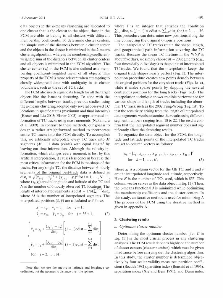
The interpolated TC tracks retain the shape, length,

and geographical path information covering the TC

tracks. Because the mean TC lifetime in the WNP is

about five days, we simply choose M 5 20 segments (e.g.,

four times daily 3 five days) as the points of interpolated

TC tracks. We found that the interpolation keeps the

original track shapes nearly perfect (Fig. 1). The inter-

polation procedure creates new points densely between

the original positions for the very short tracks (Figs. 1a–c),

while it make sparse points by skipping the several

contiguous positions for the long tracks (Figs. 1e,f). The

interpolation technique shows credible performance for

various shape and length of tracks including the abnor-

mal TC track such as the 2002 Fung-Wong (Fig. 1d). To

test the sensitivity arising from the length of interpolated

data segments, we also examine the results using different

segment numbers ranging from 18 to 22. The results con-

firm that the interpolated segment number does not sig-

nificantly affect the clustering results.

To organize the data object for the FCM, the longi-

tude and latitude points of the interpolated TC tracks

are set to column vectors as follows:

xk

5 [~x1, ~x

2, . . . , ~x

M11, ~y

1, ~y

2, . . . , ~y

M11]T

for k 5 1, . . . , K, (3)

where xk is a column vector for the kth TC, and ~x and ~y

are the interpolated longitude and latitude, respectively.

Here K is the number of TCs used, which is 855. This

column vector serves as the data object in Eq. (1). Then,

the c-means functional J is minimized while optimizing

the membership coefficients and the cluster centers. In

this study, an iterative method is used for minimizing J.

The process of the FCM using the iterative method is

given in appendix A.

3. Clustering results

a. Optimum cluster number

Determining the optimum cluster number [i.e., C in

Eq. (1)] is the most crucial process in any clustering

analyses. The FCM result depends highly on the number

of cluster centers (cluster number), which must be given

in advance before carrying out the clustering algorithm.

In this study, the cluster number is determined objec-

tively by four scalar validity measures: partition coeffi-

cient (Bezdek 1981), partition index (Bensaid et al. 1996),

separation index (Xie and Beni 1991), and Dunn index

1 Note that we use the metric in latitude and longitude co-

ordinates, not the geometric distance over the sphere.


FIG. 1. Raw 6-hourly best tracks (thick gray line with open circles) vs interpolated tracks (black line with dots):

(a) 2000 Chanchu, (b) 2000 Wukong, (c) 2001 Trami, (d) 2002 Fung-Wong, (e) 2003 Maemi, and (f) 2004 Songda. The

number of the original 6-hourly positions is shown in the bottom-right corner of each panel.


(Dunn 1973). The formulas and detailed explanations

for these indices are given in appendix B. The partition

coefficient measures the overlapping of the fuzzy clus-

ters. The fuzzy clustering result is more optimal at the

larger value of the partition coefficient. In contrast, the

other indices (partition index, separation index, and Dunn

index) measure the degree of compactness and separa-

tion of the clusters. Smaller measures indicate better

clustering. Note that none of the measures are perfect

by themselves. Accordingly, the optimum cluster number

should be determined by synthesizing all available mea-

sures (Abonyi and Feil 2007). Figure 2 shows the values

of four scalar validity measures as a function of the

cluster number. The partition coefficient monotonic de-

creases as the cluster number increases, indicating the

optimal cluster number is two. However, the choice only

based on the partition coefficient is not recommended

because it is not directly connected to the geometrical

property of the object data (e.g., Xie and Beni 1991;

Bensaid et al. 1996). The partition index also shows a

monotonic decrease as the cluster number increases;

however, the decrease ratio becomes smaller around the

six to eight clusters. On the other hand, the separation

index and Dunn index show the lowest value at seven

clusters. Therefore, these results serve as a rationale that

the optimum cluster number is seven for fuzzy clustering

of WNP TC tracks during the TC season. It is interesting

to note that this cluster number is the same as C07a de-

spite the differences in the analysis period, season and the

cluster detection method, indicating that the WNP TC

tracks seem to have a characteristic optimum number

of clusters.

b. Characteristics of clusters

1) SPATIAL DISTRIBUTION

Figure 3 presents the seven fuzzy clusters of all WNP

TC tracks (Fig. 3h) during the TC season. The gray

depth expresses membership coefficient information.

These maps demonstrate the FCM property well in that

each cluster includes all TCs with various member-

ship coefficients ranging from the highest values near the

cluster centers to the lowest values distant from the clus-

ter centers. By definition, the sum of seven member-

ship coefficients of any TC is 1. The TC tracks around

the cluster centers show distinguishing features in their

characteristic geographical path; the four recurving pat-

terns (Figs. 3a,b,d,e), the blended pattern (Fig. 3c), the

South China Sea TCs (Fig. 3f), and the straight-moving

pattern (Fig. 3g). The average of the 855 membership

coefficients for each cluster ranges from 0.09 (C5) to 0.19

(C6). These small values are obtained because the ma-

jority of TCs for each cluster are located far from the

cluster center. Thus it would be more practical to discuss

the membership coefficient statistics of a specific cluster

after discarding the TCs that have higher membership

coefficients in other clusters.

As mentioned above, each TC is assigned to a cluster

where its membership coefficient is the largest, resulting

in seven hard clusters (C1–C7; Fig. 4). For practical

purposes, the analyses and discussions will be based on

these hard clusters hereafter; however, the membership

coefficient information will be retained in the analyses

because it is an essential factor that distinguishes the

FCM from other clustering techniques. Before proceed-

ing to the discussion of each cluster’s features, the com-

parison of the clustering result with that of C07a is a

necessity as well as a matter of interest. The seven clas-

sified patterns here are somewhat different from those of

C07a mainly because of the analysis season. C07a clas-

sified the TC tracks for all seasons, while this study fo-

cuses only on those during the active TC season. There

is no doubt that the preferred TC tracks have strong

seasonality. For example, the straight westward-moving

FIG. 2. Response of four scalar validity measures to an increase in

the number of clusters: (a) partition coefficient, (b) partition index,

(c) separation index, and (d) Dunn index.


FIG. 3. (a)–(g) Seven fuzzy clusters of 855 TC tracks during the TC season and (h) all the tracks before the FCM is

done. The thick tracks are the cluster centers. The gray depth for each track is based on its membership coefficient to

a cluster.


FIG. 4. (a)–(g) Resultant seven hard clusters after assigning a TC to a cluster where its membership coefficient is

the largest. The number of TCs for each cluster is shown in the bottom-right corner of each panel. Also shown in

parentheses is the percentage of TCs for each cluster to the total number of TCs.


pattern with long trail (e.g., cluster F of C07a) seldom

occurs during the TC season so it does not appear as

a separate cluster here. Instead, the recurving patterns

are fragmented more so that the five recurving patterns2

are emerged here, compared to the four in C07a. C1

(Fig. 4a) and C3 (Fig. 4c) correspond to cluster A of C07a,

whereas C4 (Fig. 4d) and C5 (Fig. 4e) here are projected

onto the cluster C in C07a. As far as the recurving tracks

are concerned, they are apparently clustered better than

those of C07a in terms of the coherence within clusters.

This may arise from confining the analysis season to the

TC season.

C1 is characterized by many of the TCs that develop

around the northernmost part of the Philippine Sea,

recurve in and around the East China Sea with a more

north-oriented track and finally hit the East Asian region,

especially the Korean Peninsula and Japan (Fig. 4a).

Of TC season storms, 16% (133/855) have the largest

membership coefficient in C1. The TCs near the center

of C2, which develop over the southeastern region of the

WNP basin, move rather straight northwestward before

recurving south of Japan (Fig. 4b). Of the seasonal TCs,

14% (120/855) belong to C2. Because they develop over

the far open ocean close to the equator, they naturally

have the longest mean lifetime compared to those in

other clusters (Table 2). While some of them hit south-

ern Japan, the others pass through the east of Japan. The

TCs that develop slightly south of the region of devel-

opment of C1 storms in the Philippine Sea are repre-

sentative of C3 (Fig. 4c). They move straight with rather

west-oriented tracks and then strike Taiwan and the

southeastern coast of mainland China. C3 also includes

the TCs that recurve toward the Korean Peninsula and

Japan as C1 with their overall recurving latitudes about

58 south of those in C1. C3 is the second largest cluster,

including 18% (150/855) of the analyzed TCs.

The next two clusters (C4 and C5) consist of recurving

tracks over the open ocean east of Japan (Figs. 4d,e). C4

and C5 are relatively rare clusters that encompass 11%

(92/855) and 9% (79/855) of the analyzed TCs, respec-

tively. While the center of C4 is located offshore east of

Japan, that of C5 lies farther to the east. Most TCs in C4

are north-oriented so they recurve quickly after devel-

opment. The TCs near the center of C5 are also recurv-

ing ones but many of them show irregular shapes. C5

also includes the TCs that migrated from the central

North Pacific.

The center of C6 characterizes the straight-moving and

irregular tracks that are well confined to the South China

Sea (Fig. 4f). Most of the TCs hit northern Vietnam and

the southern China coastal regions. C6 includes 158 TCs

(i.e., 19% of the analyzed storms), resulting in the most

frequent pattern among the seven clusters. Last, C7 is

represented by 123 TCs (i.e., 14% of the analyzed storms)

with westward straight-moving tracks (Fig. 4g) that de-

velop over the southernmost part of the Philippines Sea,

traverse the Philippines, and make landfall over regions

similar to those of C6.

2) MEMBERSHIP COEFFICIENT STATISTICS

Figure 5 demonstrates the statistical properties of

membership coefficients for each cluster. Although the

statistics are obtained using the membership coefficients

only for the hard clusters, a considerable portion of

small membership coefficients still exists for all clusters.

This again reflects the fuzziness of the TC track data.

The boxes bounded by the lower and upper quartiles,

medians, and means in C1–C4 are located relatively

lower than those in C5–C7. For C1–C4, more than half

of the TCs belong to the clusters with membership co-

efficients less than 0.5, while for C5–C7, more than half

of TCs have membership coefficients more than 0.5.

TABLE 2. Mean values of the lifetime, traveling distance, mini-

mum central pressure, and genesis location for the TCs in seven

hard clusters and all TCs.

Life

time

(days)

Traveling

distance

(km)

Minimum

central

pressure (hPa)

Genesis

location

Longitude

(8E)

Latitude

(8N)

C1 5.0 2372 966.7 135.1 22.6

C2 7.7 3897 938.2 152.9 13.3

C3 5.6 2394 957.5 133.0 17.2

C4 5.8 2851 963.9 147.7 20.6

C5 4.8 2444 972.5 162.3 24.3

C6 3.0 998 982.4 115.8 17.1

C7 6.2 2741 952.5 134.3 13.0

All TCs 5.4 2447 962.2 137.3 17.9

FIG. 5. Box and whisker plots using the membership coefficients

for seven hard clusters. Dots indicate maximum and minimum

values.

2 C3 is included though it is a blended pattern of the straight-

moving and recurving TCs.


Moreover, the medians for C1–C4 are smaller than their

means, while the medians for C5–C7 are almost com-

parable to their mean, implying that membership co-

efficients for C1–C4 are skewed toward lower values.

These properties indicate that C1–C4 are fuzzier than

C5–C7. A relatively larger portion of TCs in C1–C4 may

be relocated if the input TC data are adjusted. The ques-

tion arises why C1–C4 are fuzzier than C5–C7. Consid-

ering that all clusters are distributed in space without

clear boundaries, it could be primarily due to the geo-

graphical locations of the two groups. C1–C4 include

TC tracks distributed near the climatological average of

the map of all tracks, whereas C5–C7 consist of those

passing near the edge of the region of typical tracks (Fig. 3).

C1–C4 have neighboring clusters on their left- and right-

hand sides, so that their membership coefficients may

disperse toward both sides. In contrast, C5–C7 only have

a neighboring cluster on one side. Thus the TC tracks

located toward the outer edge where no neighboring

cluster exists can have larger membership coefficients,

compared to those with a neighboring cluster. Recalling

that the c-means functional [Eq. (1)] is subject to two

constraints with regard to the membership coefficient—

mik $ 0 and �C

i51mik 5 1—the membership coefficients

for tracks amid several cluster centers should be smaller.

This is also shown in Figs. 3e–g. It is notable that C5 has

larger membership coefficients in general even though

it is a widely scattered cluster, which is because it lies at

the eastern boundary of the WNP. Although C1–C4 are

fuzzier based on the membership coefficient statistics,

they are significant per se because each cluster’s tracks

clearly show a distinguishable feature in terms of geo-

graphical path and track shape.

3) MEAN PROPERTIES AND MONTHLY

DISTRIBUTION

The lifetime, traveling distance, minimum central pres-

sure, and mean genesis location for each cluster are given

in Table 2. The mean lifetime is 5.4 days, the traveling

distance is 2447 km, the mean minimum central pres-

sure is 962.2 hPa, and the mean genesis location is

17.98N, 137.38E for all 855 TCs. The lifetime, traveling

distance, and minimum central pressure are closely re-

lated. Clusters (e.g., C2, C4, and C7) with relatively lon-

ger lifetime also have longer traveling distances and are

generally stronger than those with a shorter lifetime (e.g.,

C1, C5, and C6). It follows that long-lasting storms have

enough time to develop over the warm sea surface be-

fore hitting land or undergoing extratropical transition.

As the mean motion of TCs moves toward the north-

west, it is conceivable that a storm formed farther to the

east or south has the potential to last longer and develop

more intensely. This hypothesis has been proposed and

confirmed by previous literature (Camargo and Sobel

2005; Chan 2008). In this study, C2 is the representative

pattern that supports this hypothesis. It develops in the

far southeast and shows the longest lifetime and trav-

eling distance and the strongest mean intensity among

the seven clusters. In contrast, the clusters containing

TCs that developed in the west or north show a tendency

to have shorter lifetimes and traveling distances, as well

as weaker intensities. For example, C6, the cluster that

develops the farthest west (the closest to land) has the

shortest lifetime and traveling distance and the weakest

intensity among the seven clusters.

TC activity in the WNP has an apparent seasonality

not only in genesis frequency but also in the track and

genesis location. First, straight movers are more fre-

quently seen during the early or late seasons, whereas

recurving TCs prevail during the peak TC season (July,

August, and September). Second, the mean genesis po-

sition migrates northward from June through August, but

moves back to the southeast in September. These sea-

sonal variations are ascribed to variations in the position

of the monsoon trough and the North Pacific subtropical

high (NPSH) (Chia and Ropelewski 2002). Such varia-

tions are shown in Fig. 6, which summarizes monthly

genesis distributions for each cluster. The clusters about

recurving TCs (C1, C3, C4, and C5) show a peak genesis

frequency in August or September except for C2, which

shows a monotonic increase from June through October.

C6, which is the cluster of TCs formed within a deep

monsoon trough, also shows a peak during the peak TC

season. This may be because its genesis is highly related

to the active monsoon trough. It is also notable that C4

and C5, which are the clusters consisting of TCs traveling

over the open ocean, are inactive in June. In contrast, C3,

C6, and C7, which are the clusters that include straight-

moving TCs, are active in June. C7, which follows a gen-

uine straight-moving pattern, has double peaks in July

and October.

4) TC LANDFALLS AND TC-INDUCED RAINFALL

It is no wonder that TC landfall is highly dependent

upon TC track. The map of classified TC tracks (Fig. 4)

shows that TCs make landfall in different regions for

each cluster. For a quantitative analysis of the TC landfalls

for each cluster, the frequency of TC landfalls is examined

by dividing the WNP coastal area into seven subregions:

the Philippines, Vietnam, southern China (south of 258N),

eastern China, Taiwan, the Korean Peninsula, and Japan

(Table 3). For simplicity, the number of TC landfalls is

counted when the TC’s center crosses the coastal line of

the mainland of each country. The landfalls in the attached

islands (e.g., Jeju Island in South Korea, Hainan Island in

China, and Ryukyu Islands in Japan) are not counted. This


might make the number of TC landfalls be less than that

counted by the meteorological agencies [see Fig. 4 of Kim

et al. (2008) to ascertain the landfall domain].

Most TCs in C1–C3 make landfall in the East Asian

regions (e.g., the Korean Peninsula, Japan, eastern coast

of China, and Taiwan). C1 includes more than half of the

TCs that hit the Korean Peninsula (14 among a total 23

of landfalls, ;61%) and Japan (53 among a total of 96

landfalls, ;55%), while its landfalling TCs have the most

dominant influence on Japan. Once TCs in C2 make

landfall, the region is almost always Japan (27 among 34

landfalls). C2 contributes 28% of Japanese TC landfalls,

which is the second highest percentage. TCs making

landfall in Taiwan and eastern China mainly belong to

C3: 66% (35/53) for east China and 81% (51/63) for

Taiwan. C3 explains the second highest percentage (26%)

of TC landfalls on the Korean Peninsula, though the actual

frequency is small.

C6 and C7 include TCs that make landfall in South-

east Asian regions (e.g., southern coast of China, the

FIG. 6. Monthly mean number of TCs (NTC) for (a)–(g) seven hard clusters and (h) all TCs.


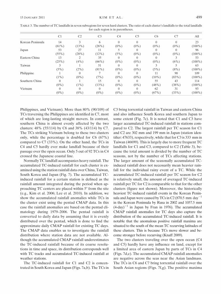
Philippines, and Vietnam). More than 80% (90/109) of

TCs traversing the Philippines are identified in C7, most

of which are long-lasting straight movers. In contrast,

southern China is almost evenly affected by the two

clusters: 48% (55/114) by C6 and 38% (43/114) by C7.

The TCs striking Vietnam belong to these two clusters

only, while the percentage is doubled for C6 (67%)

compared to C7 (33%). On the other hand, the TCs in

C4 and C5 hardly ever make landfall because of their

passage over the open ocean. Only 5 out of 92 TCs in C4

crossed the Japanese coastal line.

Normally TC landfall accompanies heavy rainfall. The

accumulated TC-induced rainfall for each cluster is ex-

amined using the station rainfall data over China, Taiwan,

South Korea and Japan (Fig. 7). The accumulated TC-

induced rainfall for a certain station is defined as the

rainfall amount integrated during the period when ap-

proaching TC centers are placed within 58 from the site

(e.g., Kim et al. 2006; Lee et al. 2010). In addition, we

show the accumulated rainfall anomalies while TCs in

the cluster exist using the pentad CMAP data. In this

case the rainfall anomalies are based on the pentad cli-

matology during 1979–2006. The pentad rainfall is

converted to daily data by assuming that it is evenly

distributed over the pentad, which is done to find the

approximate daily CMAP rainfall for existing TC days.

The CMAP data enables us to investigate the rainfall

distribution where station data are not available. Al-

though the accumulated CMAP rainfall underestimates

the TC-induced rainfall because of its coarse resolu-

tions in time and space, its distribution corresponds well

with TC tracks and accumulated TC-induced rainfall at

weather stations.

The TC-induced rainfall for C1 and C2 is concen-

trated in South Korea and Japan (Figs. 7a,b). The TCs in

C3 bring torrential rainfall in Taiwan and eastern China

and also influence South Korea and southern Japan to

some extent (Fig. 7c). It is noted that C1 and C3 have

larger accumulated TC-induced rainfall in stations com-

pared to C2. The largest rainfall per TC season for C1

and C2 are 302 mm and 199 mm in Japan (station iden-

tifier: 47633), respectively, while that for C3 is 333 mm in

Taiwan (46699). This is largely due to more frequent TC

landfalls for C1 and C3, compared to C2 (Table 3), be-

cause the total amount is divided by the number of TC

seasons, not by the number of TCs affecting stations.

The larger amount of the seasonally accumulated TC-

induced rainfall does not necessarily mean heavier rain-

fall for the individual rainy event of a TC. While the

accumulated TC-induced rainfall per TC season for C2

is relatively small, the amount of averaged TC-induced

rainfall per TC for C2 is comparable to that for the other

clusters (figure not shown). Moreover, the historically

heaviest TC-induced rainfall events in the Korean Penin-

sula and Japan were caused by TCs in C2 (870.5 mm day21

in the Korean Peninsula by Rusa in 2002 and 1057.5 mm

(4-day)21 in Japan by Fran in 1976). The accumulated

CMAP rainfall anomalies for TC days also capture the

distribution of the accumulated TC-induced rainfall. It is

notable that the anomalous positive rainfall maxima are

situated to the south of the mean TC recurving latitudes of

these clusters. This is because TCs move slower and be-

come stronger before recurving (Knaff 2009).

The two clusters traveling over the open ocean (C4

and C5) hardly have any influence on land, except for

a limited area of eastern Japan by parts of TCs in C4

(Figs. 7d,e). The accumulated CMAP rainfall anomalies

are negative across the seas near the Asian landmass.

The TCs in C6 and C7 bring torrential rainfall over the

South Asian regions (Figs. 7f,g). The positive maxima

TABLE 3. The number of TC landfalls in seven subregions for seven hard clusters. The ratio of each cluster’s landfalls to the total landfalls

for each region is in parentheses.

C1 C2 C3 C4 C5 C6 C7 All

Korean Peninsula 14 3 6 0 0 0 0 23

(61%) (13%) (26%) (0%) (0%) (0%) (0%) (100%)

Japan 53 27 11 5 0 0 0 96

(55%) (28%) (12%) (5%) (0%) (0%) (0%) (100%)

Eastern China 13 2 35 0 0 0 3 53

(25%) (4%) (66%) (0%) (0%) (0%) (6%) (100%)

Taiwan 3 1 51 0 0 3 5 63

(5%) (2%) (81%) (0%) (0%) (5%) (8%) (100%)

Philippine 1 0 7 0 0 11 90 109

(1%) (0%) (7%) (0%) (0%) (10%) (83%) (100%)

Southern China 0 1 15 0 0 55 43 114

(0%) (1%) (13%) (0%) (0%) (48%) (38%) (100%)

Vietnam 0 0 0 0 0 62 31 93

(0%) (0%) (0%) (0%) (0%) (67%) (33%) (100%)


FIG. 7. The mean of the accumulated TC-induced rainfall [mm (TC season)21] (circles) for the TCs in seven hard

clusters. Also plotted are the mean of the CMAP rainfall anomalies [mm (TC season)21] (shading) integrated over

TC existing days for each cluster.


of the accumulated CMAP rainfall anomalies are lo-

cated east and west of the Philippines. The accumulated

TC-induced rainfall has its largest value at Hainan Island

(59855) [236 mm (TC season)21] for C6 and southern

Taiwan (46766) [250 mm (TC season)21] for C7. From

the rainfall distribution, we can infer that C6 induces

more rainfall over southern China and Vietnam, while

C7 leads to more rainfall over the Philippines. This is

consistent with TC tracks and the landfall statistics for

these clusters (Fig. 4 and Table 3).

4. Large-scale environment

In this section, we try to find deterministic large-scale

environmental patterns associated with TCs for each

cluster. Similarly to C07b, we plot composite anomalies

of the SST, low-level winds (Fig. 8), and composite totals

of steering flows (Fig. 9) for each cluster. However, in

this study, the membership coefficients are applied as

weighting factors to the composite analysis to give more

weights to the TCs that are closer to cluster centers:

FIG. 8. Membership coefficient-weighted composites of the SST (shading), 850-hPa wind (vector), and relative

vorticity anomalies (black contour) on the day of TC genesis for (a)–(g) the TCs in seven hard clusters and (h) all TCs.

Only significant values at 5% level are plotted for the wind and vorticity fields. The gray contours are drawn for the

SST anomaly significant at 5% level.


FIG. 9. Membership coefficient-weighted composites of the tropospheric-layer mean flows (streamline, m s21) on

the day of TC genesis for the TCs in seven hard clusters. The color depth for streamlines represents the mean wind

speed. The solid contour is the 5880 gpm of the 500-hPa geopotential height composite. Also shown is the mean track

for each cluster (red line).


Xi5

�K

i

k51m

ikX

k

�K

i

k51m

ik

, (4)

where Xiis the composite of a field X for the ith cluster,

Xk is the field associated with kth TC, mik is the mem-

bership coefficient of the kth TC to the ith cluster, and Ki

is the TC number assigned to an ith hard cluster. The

results from the nonweighted composites are very sim-

ilar to those from the weighted composites. This may be

because the composites are obtained using the TCs in-

cluded in each hard cluster or because the variability of

large-scale environments within a cluster is not very large.

Nevertheless, it is reasonable to think that the weighted

composite should improve the representation of large-

scale environments associated with a cluster center.

As in C07b, composites are constructed only for the

first position of TCs. C07b suggested that composites

based on an initial position are better for potential use

of these patterns in tracks and landfall forecasts. Thus,

once various relations between TC track patterns and

large-scale environmental fields in the initial developing

stage are established, they may be applied to predict the

probable track pattern of TCs in a specific region.

a. SST and low-level circulation

Figure 8 shows the membership coefficient-weighted

composite anomalies of the SST, horizontal winds, and

relative vorticity at 850 hPa on the day of TC genesis.

Weekly SSTs are linearly interpolated to a daily time

scale to approximate the SST pattern on the day of TC

genesis. The mean TC genesis region of a cluster is

marked with a filled circle. For all clusters, significant

SST anomalies are located outside of TC genesis regions.

The composite of SST anomalies on the day of TC gen-

esis can originate either from a background thermal

forcing affecting TC genesis, a transient wave response

induced by TC-related convective heating, or a local at-

mospheric and oceanic state independent of TC. As

shown in the figure, local SST anomalies in a TC genesis

area do not deviate significantly from the climatology

except for those associated with C5. Instead, significant

anomalies spread across the equatorial Pacific through

the North Pacific Ocean.

For C1 and C2, the composite SST anomalies in the

tropics somewhat resemble El Nino–related anomalies

(Figs. 8a,b). In relation to C1, cold SST anomalies spread

over the equatorial central and eastern Pacific, which are

similar to those during La Nina periods. These anomalies

are thought to be a background state that is not induced

by TCs in that they are decoupled from low-level cir-

culations around the mean TC genesis center. On the

other hand, in the midlatitudes significant positive SST

anomalies are found from the Yellow Sea through the

Kuroshio extension. Those across the Korean Peninsula

through off the east of Japan could potentially be caused

by a low-level anticyclonic wave response there, whereas

those along the Kuroshio extension are, though it is

rather unclear, likely due to a local environmental state.

In contrast to C1, there are two bands of warm SST

anomalies in the composite of C2 (Fig. 8b); one is over the

equatorial central and eastern Pacific, and the other

elongates from the date line toward the west coast of

North America. The Pacific Rim is generally warm ex-

cept along the western boundary where patches of sig-

nificant cold SST anomalies are seen. The strong 850-hPa

anomalous westerlies are significant south of the mean

TC genesis center along the equatorial western Pacific,

which form cyclonic shear vorticity to the north, favoring

TC genesis there. Conversely, the anomalous westerly

winds can be interpreted as a manifestation of TC-

related circulation as well. In any case these flows are

consistent with the zonal SST gradient.

The composite map for C3 characterizes positive SST

anomalies over the equatorial central Pacific (CP) with

negative anomalies both west and east of the anomalies,

as well as those appearing in a horseshoe-like pattern in

the North Pacific Ocean (Fig. 8c). The tropical pattern is

reminiscent of the new type El Nino that is referred to as

the El Nino Modoki or the CP–El Nino (e.g., Ashok

et al. 2007; Kao and Yu 2009; Kug et al. 2009; Yeh et al.

2009). The correlation between the seasonal TC number

in C3 and the seasonal mean El Nino Modoki index

(Ashok et al. 2007) is 0.4, which is significant at the 99%

confidence level, while the correlation with the Nino 3.4

index is 0.22, which is statically insignificant. It is likely

that the CP–El Nino type SST pattern acts as a back-

ground forcing favoring C3. The C07b also showed the

separation of two types of El Nino–related clusters: one

related to the typical El Nino and the other to CP–

El Nino. Yeh et al. (2009) suggested that the CP–El Nino

events would increase in a warmer climate. Thus, it will

be interesting to see whether this cluster increases under

global warming. Interestingly, the midlatitude SST anom-

alies in the North Pacific Ocean are also positive like those

related to C1, which we interpret as a transient related to

TCs as in C1 because they should be negative in associa-

tion with the CP–El Nino event (Ashok et al. 2007).

For C4 and C5, which have two recurving patterns that

have little influence on land areas, significant positive

SST anomalies are found in the midlatitude North Pa-

cific Ocean (Figs. 8d,e). In particular, C5 shows a strong

teleconnection pattern throughout the North Pacific,


which supports the hypothesis that the SST anomalies

could potentially come from the TC-induced wave re-

sponse. Next, C6 shows a strong cyclonic cell over the

South China Sea that seems like a TC-related vortex. It

is also possibly associated with the monsoon trough that

induces a positive vorticity over the South China Sea.

Also of interest are wavelike SST anomalies from the

East China Sea through the North Pacific Ocean. Along

the axis of the wave, the neighboring anticyclonic and

warm anomalies centered over the East China Sea likely

indicate the westward expansion of the NPSH. Last, C7

also shows anomalies of anticyclonic winds and warm

SST in the north of a genesis region. This indicates that

the strong NPSH guides the TCs in this cluster to move

straight westward.

In summary, the seven clusters can be grouped into

two broad types in the context of their relation with the

Pacific SSTs. C1–C3, which are generated by forcing

from background mean states (i.e., tropical SST anom-

alies), are included in one group. C4–C7 are included

in a second group that does not show any significant

background mean state in the tropics In addition, an in-

teresting feature in the composite based on the day of TC

genesis is the warm SST anomalies in the midlatitudes

(Fig. 8h). This may be caused by a potential TC-induced

response affecting the North Pacific climate but the de-

tailed analysis on their causality is beyond the scope of

this study.

b. Steering flows

A TC’s motion results from complex interactions be-

tween internal dynamics (i.e., beta drift) and external

influences (Chan 2005). Environmental steering is the

most dominant external influence and accounts for up to

80% of TC motion (Holland 1993), which is defined as

pressure-weighted vertically averaged horizontal winds

in the troposphere (also referred to as tropospheric-

layer mean flows):

Vtrop

51

p0� p

ðp0

p

V dp, (5)

where p0 is the bottom level and p is the top level. In this

study, p0 and p are set at 850 and 200 hPa, respectively,

following the previous studies (Chan and Gray 1982;

Kim et al. 2005b, 2008).

Figure 9 shows streamlines for the membership

coefficient-weighted composites of the tropospheric-layer

mean flows based on the day of TC genesis for each

cluster. Also shown are the composites of the 5880 gpm

at 500 hPa that represent the influence of the NPSH.

The composite with respect to the day of TC genesis

cannot explain the each cluster’s mean track perfectly

because a TC interacts continuously with its synoptic

environments as it moves. In a climatological sense,

however, it can be proposed that the composite of many

events may effectively filter out transients so that it can

reveal characteristics that are slowly varying large-scale

environments that are persistent for several days. With

this assumption, the composited pattern for the genesis

day can be related to the cluster’s mean track. To some

extent, the validity of this assumption is supported by

Fig. 9 in that the cluster’s mean track follows the flows

steered by the NPSH. However, the beta drift seems not

negligible in that the mean tracks are deflected north-

ward for all the clusters.

The mean tracks of C1 and C7 are well explained by

the strong southeasterlies and easterlies around the south-

west of the NPSH, respectively (Figs. 9a,g), whereas

those of C4 and C5 penetrate through the weak western

boundary of the NPSH owing to weak flow speeds (Figs.

9d,e). The beta drift is more apparent for the tracks that

drift on weak steering backgrounds. These two contrast-

ing groups of clusters emphasize the dominant role of the

environmental steering in TC motion. This may also in-

dicate that the patterns of the environmental steering

flows are relatively well sustained in these clusters during

TC lifetime, which supports the validity of the assump-

tion made. The mean tracks in C2 and C3 follow the

direction of the strong environmental steering flows

around the south and southwest of the NPSH, respectively

(Figs. 9b,c). However, even in the early stage the mean

tracks for C2 and C3 are diverted more to the right of the

steering flows compared to C1, even though the steering

flows are as strong as those for C1. Although the reason

is not clear, we may suggest one possibility; that is, the

stronger beta effect for more intense TCs based on the

experiments of Carr and Elsberry (1997).

5. Summary and discussion

a. Summary

This study has shown the usefulness of the fuzzy

clustering technique to classify TC tracks. Fuzzy clus-

tering has been known to produce more natural classi-

fication results for datasets such as TC tracks that are too

complex to determine their boundaries of distinctive pat-

terns. In this study, the fuzzy c-means clustering method,

which has been widely used for data clustering, was used

to group 855 TC tracks over the WNP during TC seasons

for the period of 1965–2006. Cross validation of four

validity measures—including the partition coefficient,

partition index, separation index, and Dunn index—

identified seven clusters (C1–C7) as the optimum num-

ber (Fig. 2). The principle of the FCM leads all the seven


clusters to include all TCs with different membership

coefficients (Fig. 3). For practical purposes, each TC was

assigned to a cluster where its membership coefficient is

the largest (Fig. 4).

Each cluster showed distinctive characteristics in its

lifetime, traveling distance, intensity, and monthly dis-

tribution. The clusters that consist of TCs with longer

lifetime and traveling distance had stronger intensity

(Table 2). For example, C2 (C6) is characterized by the

longest (shortest) lifetime and traveling distance as well

as the strongest (weakest) intensity among clusters. The

monthly frequency distribution demonstrated the sea-

sonal variations in genesis locations and tracks that arise

from those in the monsoon tough and NPSH (Fig. 6).

Naturally, the main landfalling regions and the dis-

tribution of TC-induced rainfalls are dependent on track

patterns. The TCs in C1–C3 made landfall in the East

Asian regions (i.e., the Korean Peninsula, Japan, eastern

China, and Taiwan) with heavy rainfall, while those in

C6–C7 hit the South Asian regions (i.e., Philippines,

Vietnam, and southern China) (Table 3). For each clus-

ter, the geographical distribution of TC-induced rainfall

matched the cluster’s tracks and main landfalling regions

well (Fig. 7).

The related large-scale environments were analyzed

by the composite of the oceanic and atmospheric pa-

rameters on the day of TC genesis. Each cluster showed

different features in the SST and low-level circulation

anomalies in association with the main TC genesis re-

gion (Fig. 8). In particular, the tropical SST variations

were significantly related to TC activity in C1, C2 and

C3, representing the influences of La Nina, El Nino, and

CP–El Nino, respectively. The tropospheric-layer mean

winds represented the steering flows determining the

cluster-averaged TC movement well. The west-oriented

tracks were explained by the easterlies around the south-

west periphery of the NPSH, while the north-oriented

tracks penetrating the weak western boundary of the

NPSH were associated with the weak steering flows.

b. Discussion

Instead of producing hard clusters directly, the FCM

performs soft clustering to find the cluster centers and

membership coefficients of each object to all cluster cen-

ters. The membership coefficient is qualitatively similar

to the membership probability of the mixture regression

model suggested by C07a. This property seems to make

the FCM can be an alternative to C07a.

The fuzzy clustering technique has been utilized in

several previous studies to classify large-scale circulation

patterns as well as TC tracks (e.g., Harr and Elsberry

1995a; Kim 2005). Both studies employed a vector em-

pirical orthogonal function (EOF) analysis as a data

initialization process and transformed the c-means func-

tional [Eq. (1)] into an applicable form for the co-

efficients from the vector EOF analysis. In this study, the

data initialization process was simplified; that is, the lon-

gitude and latitude information is directly put in the FCM

algorithm.

To use the longitude and latitude information di-

rectly for the FCM input, all the data objects should be

of equal length, which is critical for c-means clustering

family (including k-means clustering). Because of this

constraint, previous studies could not use the whole track

information (Blender et al. 1997; Elsner and Liu 2003;

Elsner 2003). To overcome this limitation, this study

proposed a simple direct interpolation with an equal

number of segments for all tracks by leaving out time

information of the best-track data. This method can

preserve the shape of the entire track quite well (Fig. 1)

and allows them to be put in as an input for the c-means

clustering family. This artificial interpolation is justified

in the sense that the clustering result was reasonable,

which, in turn, implies that the most critical information

is the track shape. This method makes the FCM de-

signed here more straightforward and easier to apply to

the clustering analysis of tracks. This direct interpola-

tion can be an alternative to the mass moments sug-

gested by Nakamura et al. (2009).

We also applied the k-means clustering to the same

dataset for the purpose of comparison. The k-means

clustering resulted in somewhat different clusters espe-

cially in the recurving tracks (figure not shown). For in-

stance, the El Nino–related pattern (i.e., C2) was divided

into two clusters and C1, C4, and C5 were relocated into

two clusters. As a result, the population of each cluster

became more unbalanced in the k means compared to

the FCM.3 This is caused by the difference in fundamentals

between the two similar but different methods (see Table

1). Although the results by the FCM are more balanced and

useful in isolating influences of the physical phenomena

such as El Nino, La Nina, and CP–El Nino on the TC ac-

tivity, it is not correct to say one is superior to the other

because the results are dependent on the data property.

In addition, the FCM using all season TC tracks (i.e.,

1128 TCs for 1965–2006) were examined and identified

eight clusters as the optimum cluster number. The eight

clusters consist of seven patterns similar to those from

the tracks during TC season and the one cluster that

includes both recurvers at lower latitude and straight

movers formed farther southeast of the WNP (figure not

3 The ratio of the largest to the smallest number of TCs is 2.8

(152/52) for the k-means result, whereas it is 1.9 (150/79) for the

FCM result.


shown). We conclude that the seven clusters are, to a

large extent, robust patterns by the FCM.

A weakness in the FCM is that it is an unsupervised

clustering algorithm that gives different clustering re-

sults when the input data are changed. However, in the

case of the newly observed TCs, they can be allocated

into the existing clusters without recalculation by using

the following procedures. First, interpolate the new TC

tracks into the same number of segments. Next, calcu-

late their membership coefficients to the existing cluster

centers. Finally, allocate them to the clusters where their

membership coefficients are largest. With this method

the existing clusters of TC track patterns can be preserved.

It has been reported that the various atmospheric

modes such as the quasi-biennial oscillation (QBO) and

MJO modulate TC tracks over the WNP (e.g., Ho et al.

2009b; Kim et al. 2008). Although it was not discussed

here, the fingerprint of these phenomena also appears

in the clustered TC tracks. The correlation between the

seasonal TC number in C4 and the seasonal mean 50-hPa

zonal wind index for the QBO during 1979–2006 reaches

20.62, representing more activity of C4 during the east-

erly QBO season (Ho et al. 2009b). The statistical re-

lation with the atmospheric and oceanic modes along

with large-scale environments may be applicable to the

long-range prediction of TC tracks. Some recent studies

successfully predicted seasonal TC activity over the spe-

cific region in the WNP using statistical methods based on

the antecedent large-scale environments (Chu and Zhao

2007; Chu et al. 2007; Ho et al. 2009a; Kim et al. 2010). If

the classified patterns can be predicted using a simi-

lar method, the long-range forecast for the regional TC

activity covering the entire WNP is promising. The de-

velopment of this prediction technique will be discussed

in a separate paper. Moreover, the clustering can also be

applied to diagnose the future change of TC tracks and

the probability of landfall under global warming using

high-resolution model scenario experiment.

Acknowledgments. This work was funded by the Korea

Meteorological Administration Research and Develop-

ment Program under Grant CATER 2006-4204. H.-S.

Kim was also supported by the BK21 project of the Ko-

rean government. J.-H. Kim was supported by NSC99-

2811-M-002-076.

APPENDIX A

Iterative Method for Minimizing Fuzzy c-MeansFunctional

Given the dataset x, choose the number of clusters 1 ,

C , K, the weighting exponent m . 1, the termination

tolerance « . 0, and the partition matrix U:

U 5

m1,1

m1,2

� � � m1,C

m2,1

m2,2

� � � m2,C

..

. ... . .

. ...

mK,1

mK,2

� � � mK,C

266664

377775. (A1)

Initialize the partition matrix U(0) randomly.

Repeat following steps for l 5 1, 2, . . . until kJ(l) 2

J(l21)k , «.

Step 1—Compute the cluster centers:

c(l)i 5

�K

k51(m

(l�1)ik )mx

k

�K

k51(m

(l�1)ik )m

, 1 # i # C. (A2)

Step 2—Update the partition matrix:

m(l)ik 5 �

C

j51

xk� c

(l)i

�� 2

xk� c

(l)j

�� 2

0@

1A

2/(m�1)264

375�1

(A3)

(Abonyi and Feil 2007).

APPENDIX B

Validity Scalar Measures for the OptimumCluster Number

The partition coefficient (Bezdek 1981) measures the

amount of overlapping between the clusters. It is com-

puted as

Partition coefficient 51

K�C

i51�K

k51m2

ik. (B1)

This index is inversely proportional to the overall av-

erage overlap between the fuzzy subsets. The main

drawback of the partition coefficient is that it is only

based on the membership coefficients. Thus, it lacks

direct connection to the geometrical properties of the

object data.

The partition index (Bensaid et al. 1996) validates

both compactness and separation of the clusters. The

compactness is represented by the mean of the distance

between the objects and the cluster center weighted by

the membership coefficients, and the separation is esti-

mated by the sum of the distances from a cluster center

to all other cluster centers. The partition index is obtained


by summing up the ratio of the compactness to the

separation, whose formula is as follows:

Partition index 5 �C

i51

�K

k51mm

ik xk� c

ik k2

�K

k51m

ik�C

j51c

j� c

ik k2

. (B2)

The separation index (Xie and Beni 1991) is also

represented by the ratio of the compactness to the sep-

aration, which is similar to the partition index. However,

the separation is defined as the minimum distance be-

tween the cluster centers. The separation index is com-

puted as

Separation index 5

�C

i51�K

k51mm

ik xk� c

ik k2

K mini, j

cj� c

ik k2. (B3)

The Dunn index (Dunn 1973) is a classical index to

identify the compact and separate clusters. This index

represents the ratio of the shortest distance between

the two objects belonging to each other cluster and the

largest distance between the two objects belonging to

the same cluster. The Dunn index can be applied only

to hard partitions. In this study, it is computed after

each object is assigned to a cluster where its member-

ship coefficient is the largest. The Dunn index is de-

fined as

Dunn index 5 min1#i#C

mini, j,C

minx

i2C

i, x

j2C

jx

i� x

jk kmax

1#k#Cmaxx

i, x

j2C

xi� x

jk k� �

8<:

9=;

8<:

9=;. (B4)

REFERENCES

Abonyi, J., and B. Feil, 2007: Cluster Analysis for Data Mining and

System Identification. Birkhauser Basel, 303 pp.

Ashok, K., S. K. Behera, S. A. Rao, H. Weng, and T. Yamagata,

2007: El Nino Modoki and its possible teleconnection. J. Geo-

phys. Res., 112, C11007, doi:10.1029/2006JC003798.

Bensaid, A. M., L. O. Hall, J. C. Bezdek, L. P. Clarke, M. L. Silbiger,

J. A. Arrington, and R. F. Murtagh, 1996: Validity-guided

(re)clustering with applications to image segmentation. IEEE

Trans. Fuzzy Syst., 4, 112–123.

Bezdek, J. C., 1981: Pattern Recognition with Fuzzy Objective

Function Algorithms. Kluwer Academic, 256 pp.

Blender, R., K. Fraedrich, and F. Lunkeit, 1997: Identification of

cyclone-track regimes in the North Atlantic. Quart. J. Roy.

Meteor. Soc., 123, 727–741.

Camargo, S. J., and A. H. Sobel, 2005: Western North Pacific

tropical cyclone intensity and ENSO. J. Climate, 18, 2996–

3006.

——, A. W. Robertson, S. J. Gaffney, P. Smyth, and M. Ghil, 2007a:

Cluster analysis of typhoon tracks. Part I: General properties.

J. Climate, 20, 3635–3653.

——, ——, ——, ——, and ——, 2007b: Cluster analysis of typhoon

tracks. Part II: Large-scale circulation and ENSO. J. Climate,

20, 3654–3676.

——, ——, A. G. Barnston, and M. Ghil, 2008: Clustering of

eastern North Pacific tropical cyclone tracks: ENSO and MJO

effects. Geochem. Geophys. Geosyst., 9, Q06V05, doi:10.1029/

2007GC001861.

Carr, L. E., and R. L. Elsberry, 1997: Models of tropical cyclone

wind distribution and beta-effect propagation for application

to tropical cyclone track forecasting. Mon. Wea. Rev., 125,

3190–3209.

Chan, J. C. L., 1985: Tropical cyclone activity in the Northwest

Pacific in relation to the El Nino/Southern Oscillation phe-

nomenon. Mon. Wea. Rev., 113, 599–606.

——, 2005: The physics of tropical cyclone motion. Annu. Rev.

Fluid Mech., 37, 99–128.

——, 2008: Decadal variations of intense typhoon occurrence in

the western North Pacific. Proc. Roy. Soc. London, 464A,

249–272.

——, and W. M. Gray, 1982: Tropical cyclone movement and sur-

rounding flow relationships. Mon. Wea. Rev., 110, 1354–1374.

Chia, H. H., and C. F. Ropelewski, 2002: The interannual variability

in the genesis location of tropical cyclones in the northwest

Pacific. J. Climate, 15, 2934–2944.

Chu, P.-S., 2002: Large-scale circulation features associated with

decadal variations of tropical cyclone activity over the central

North Pacific. J. Climate, 15, 2678–2689.

——, and X. Zhao, 2007: A Bayesian regression approach for

predicting seasonal tropical cyclone activity over the central

North Pacific. J. Climate, 20, 4002–4013.

——, ——, C.-T. Lee, and M.-M. Lu, 2007: Climate prediction of

tropical cyclone activity in the vicinity of Taiwan using the

multivariate least absolute deviation regression method. Terr.

Atmos. Ocean. Sci., 18, 805–825.

Dunn, J. C., 1973: A fuzzy relative of the ISODATA process and

its use in detecting compact well-separated clusters. Cybern.

Syst., 3, 32–57.

Elsner, J. B., 2003: Tracking hurricanes. Bull. Amer. Meteor. Soc.,

84, 353–356.

——, and K. B. Liu, 2003: Examining the ENSO–typhoon hy-

pothesis. Climate Res., 25, 43–54.

Hall, T. M., and S. Jewson, 2007: Statistical modeling of North

Atlantic tropical cyclone tracks. Tellus, 59A, 486–498.

Harr, P. A., and R. L. Elsberry, 1991: Tropical cyclone track

characteristics as a function of large-scale circulation anoma-

lies. Mon. Wea. Rev., 119, 1448–1468.

——, and ——, 1995a: Large-scale circulation variability over the

tropical western North Pacific. Part I: Spatial patterns and

tropical cyclone characteristics. Mon. Wea. Rev., 123, 1225–

1246.

——, and ——, 1995b: Large-scale circulation variability over the

tropical western North Pacific. Part II: Persistence and tran-

sition characteristics. Mon. Wea. Rev., 123, 1247–1268.


Ho, C.-H., J.-J. Baik, J.-H. Kim, D.-Y. Gong, and C.-H. Sui, 2004:

Interdecadal changes in summertime typhoon tracks. J. Cli-

mate, 17, 1767–1776.

——, J.-H. Kim, H.-S. Kim, C.-H. Sui, and D.-Y. Gong, 2005:

Possible influence of the Antarctic Oscillation on tropical cy-

clone activity in the western North Pacific. J. Geophys. Res.,

110, D19104, doi:10.1029/2005JD005766.

——, H.-S. Kim, and P.-S. Chu, 2009a: Seasonal prediction of

tropical cyclone frequency over the East China Sea through

a Bayesian Poisson-regression method. Asia-Pac. J. Atmos.

Sci., 45, 45–54.

——, ——, J.-H. Jeong, and S.-W. Son, 2009b: Influence of

stratospheric quasi-biennial oscillation on tropical cyclone

tracks in western North Pacific. Geophys. Res. Lett., 36,

L06702, doi:10.1029/2009GL037163.

Hodanish, S., and W. M. Gray, 1993: An observational analysis

of tropical cyclone recurvature. Mon. Wea. Rev., 121, 2665–

2689.

Holland, G. J., 1993: Tropical cyclone motion. Global Guide

to Tropical Cyclone Forecasting, G. J. Holland, Ed., World

Meteorological Organization, WMO/TD-560. [Available on-

line at http://www.cawcr.gov.au/bmrc/pubs/tcguide/globa_guide_

intro.htm.]

Kalnay, E., and Coauthors, 1996: The NCEP/NCAR 40-Year Re-

analysis Project. Bull. Amer. Meteor. Soc., 77, 437–471.

Kao, H.-Y., and J. Y. Yu, 2009: Contrasting eastern-Pacific and

central-Pacific types of ENSO. J. Climate, 22, 615–632.

Kaufman, L., and P. J. Rousseeuw, 1990: Finding Groups in Data: An

Introduction to Cluster Analysis. John Wiley and Sons, 342 pp.

Kim, H.-S., C.-H. Ho, P.-S. Chu, and J.-H. Kim, 2010: Seasonal

prediction of summertime tropical cyclone activity over the

East China Sea using the least absolute deviation regression

and the Poisson regression. Int. J. Climatol., 30, 210–219,

doi:10.1002/joc.1878.

Kim, J.-H., 2005: A study on the seasonal typhoon activity using the

statistical analysis and dynamic modeling. Ph.D. thesis, Seoul

National University, 187 pp.

——, C.-H. Ho, and C.-H. Sui, 2005a: Circulation features associ-

ated with the record-breaking typhoon landfall on Japan in

2004. Geophys. Res. Lett., 32, L14713, doi:10.1029/2005GL022494.

——, ——, ——, and S. K. Park, 2005b: Dipole structure of in-

terannual variations in summertime tropical cyclone activity

over East Asia. J. Climate, 18, 5344–5356.

——, ——, M.-H. Lee, J.-H. Jeong, and D. Chen, 2006: Large in-

creases in heavy rainfall associated with tropical cyclone land-

falls in Korea after the late 1970s. Geophys. Res. Lett., 33,

L18706, doi:10.1029/2006GL027430.

——, ——, H.-S. Kim, C.-H. Sui, and S. K. Park, 2008: Systematic

variation of summertime tropical cyclone activity in the western

North Pacific in relation to the Madden–Julian oscillation.

J. Climate, 21, 1171–1191.

Knaff, J. A., 2009: Revisiting the maximum intensity of recurving

tropical cyclones. Int. J. Climatol., 29, 827–837.

Kug, J. S., F. F. Jin, and S. I. An, 2009: Two types of El Nino events:

Cold tongue El Nino and warm pool El Nino. J. Climate, 22,1499–1515.

Lander, M. A., 1996: Specific tropical cyclone track types and un-

usual tropical cyclone motions associated with a reverse-oriented

monsoon trough in the western North Pacific. Wea. Forecasting,

11, 170–186.

Lee, M.-H., C.-H. Ho, and J.-H. Kim, 2010: Influence of tropical

cyclone landfalls on spatiotemporal variations in typhoon sea-

son rainfall over South China. Adv. Atmos. Sci., 27, 433–454.

Nakamura, J., U. Lall, Y. Kushnir, and S. J. Camargo, 2009: Clas-

sifying North Atlantic tropical cyclone tracks by mass mo-

ments. J. Climate, 22, 5481–5494.

Reynolds, R. W., N. A. Rayner, T. M. Smith, D. C. Stokes, and

W. Q. Wang, 2002: An improved in situ and satellite SST

analysis for climate. J. Climate, 15, 1609–1625.

Xie, P. P., and P. A. Arkin, 1997: Global precipitation: A 17-year

monthly analysis based on gauge observations, satellite esti-

mates, and numerical model outputs. Bull. Amer. Meteor. Soc.,

78, 2539–2558.

Xie, X. L., and G. A. Beni, 1991: Validity measure for fuzzy clus-

tering. IEEE Trans. PAMI, 3, 841–846.

Yeh, S.-W., J.-S. Kug, B. Dewitte, M.-H. Kwon, B. P. Kirtman, and

F.-F. Jin, 2009: El Nino in a changing climate. Nature, 461,511–514.

Zimmermann, H.-J., 2001: Fuzzy Set Theory and Its Applications.

4th ed. Kluwer Academic, 514 pp.


Documents

Pattern Classiﬁcation of Typhoon Tracks Using the Fuzzy