Title stata.com

mi impute chained — Impute missing values using chained equations

Syntax Menu Description OptionsRemarks and examples Stored results Methods and formulas AcknowledgmentsReferences Also see

Syntax

Default specification of prediction equations, basic syntax

mi impute chained (uvmethod) ivars[= indepvars

] [if] [

weight] [

, impute options options]

Default specification of prediction equations, full syntax

mi impute chained lhs[= indepvars

] [if] [

weight] [

, impute options options]

Custom specification of prediction equations

mi impute chained lhsc[= indepvars

] [if] [

weight] [

, impute options options]

where lhs is lhs spec[

lhs spec[. . .

] ]and lhs spec is

(uvmethod[

if] [

, uvspec options]) ivars

lhsc is lhsc spec[

lhsc spec[. . .

] ]and lhsc spec is

(uvmethod[

if] [

, include(xspec) omit(varlist) noimputed uvspec options]) ivars

ivars (or newivar if uvmethod is intreg) are the names of the imputation variables.

uvspec options are ascontinuous, noisily, and the method-specific options as described in themanual entry for each univariate imputation method.

The include(), omit(), and noimputed options allow you to customize the default predictionequations.

1

2 mi impute chained — Impute missing values using chained equations

uvmethod Description

regress linear regression for a continuous variable; [MI] mi impute regresspmm predictive mean matching for a continuous variable;

[MI] mi impute pmmtruncreg truncated regression for a continuous variable with a restricted range;

[MI] mi impute truncregintreg interval regression for a continuous partially observed (censored) variable;

[MI] mi impute intreglogit logistic regression for a binary variable; [MI] mi impute logitologit ordered logistic regression for an ordinal variable; [MI] mi impute ologitmlogit multinomial logistic regression for a nominal variable;

[MI] mi impute mlogitpoisson Poisson regression for a count variable; [MI] mi impute poissonnbreg negative binomial regression for an overdispersed count variable;

[MI] mi impute nbreg

impute options Description

Main∗add(#) specify number of imputations to add; required when no imputations exist∗replace replace imputed values in existing imputationsrseed(#) specify random-number seeddouble store imputed values in double precision; the default is to store them

as float

by(varlist[, byopts

]) impute separately on each group formed by varlist

Reporting

dots display dots as imputations are performednoisily display intermediate outputnolegend suppress all table legends

Advanced

force proceed with imputation, even when missing imputed values areencountered

noupdate do not perform mi update; see [MI] noupdate option

∗add(#) is required when no imputations exist; add(#) or replace is required if imputations exist.noupdate does not appear in the dialog box.

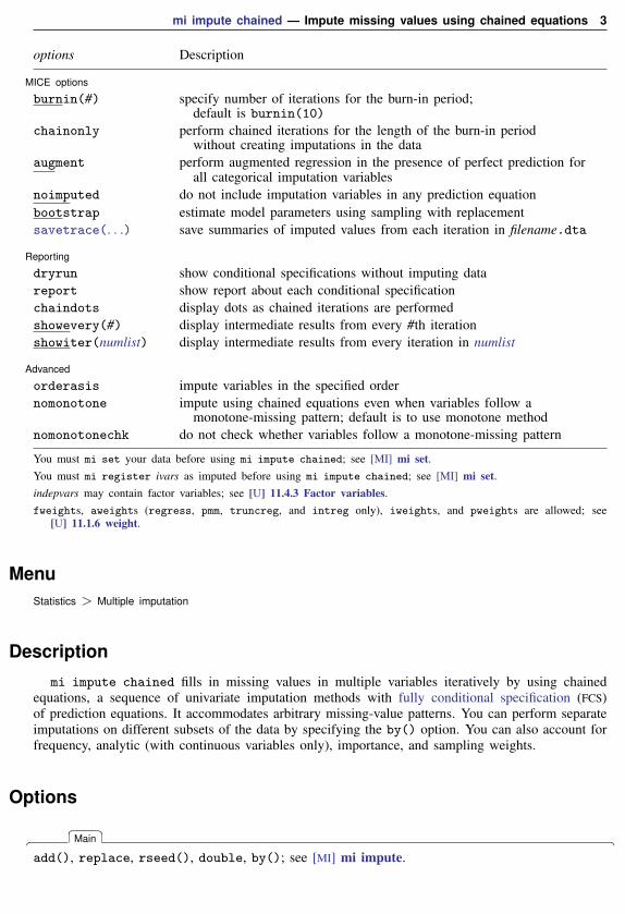
mi impute chained — Impute missing values using chained equations 3

options Description

MICE options

burnin(#) specify number of iterations for the burn-in period;default is burnin(10)

chainonly perform chained iterations for the length of the burn-in periodwithout creating imputations in the data

augment perform augmented regression in the presence of perfect prediction forall categorical imputation variables

noimputed do not include imputation variables in any prediction equationbootstrap estimate model parameters using sampling with replacementsavetrace(. . .) save summaries of imputed values from each iteration in filename.dta

Reporting

dryrun show conditional specifications without imputing datareport show report about each conditional specificationchaindots display dots as chained iterations are performedshowevery(#) display intermediate results from every #th iterationshowiter(numlist) display intermediate results from every iteration in numlist

Advanced

orderasis impute variables in the specified ordernomonotone impute using chained equations even when variables follow a

monotone-missing pattern; default is to use monotone methodnomonotonechk do not check whether variables follow a monotone-missing pattern

You must mi set your data before using mi impute chained; see [MI] mi set.You must mi register ivars as imputed before using mi impute chained; see [MI] mi set.indepvars may contain factor variables; see [U] 11.4.3 Factor variables.fweights, aweights (regress, pmm, truncreg, and intreg only), iweights, and pweights are allowed; see

[U] 11.1.6 weight.

MenuStatistics > Multiple imputation

Description

mi impute chained fills in missing values in multiple variables iteratively by using chainedequations, a sequence of univariate imputation methods with fully conditional specification (FCS)of prediction equations. It accommodates arbitrary missing-value patterns. You can perform separateimputations on different subsets of the data by specifying the by() option. You can also account forfrequency, analytic (with continuous variables only), importance, and sampling weights.

Options

� � �Main �

add(), replace, rseed(), double, by(); see [MI] mi impute.

4 mi impute chained — Impute missing values using chained equations

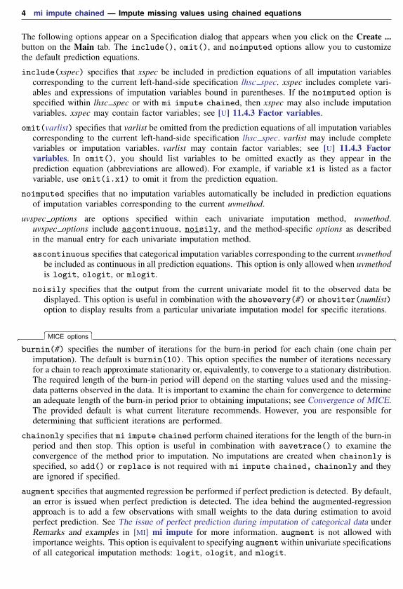
The following options appear on a Specification dialog that appears when you click on the Create ...button on the Main tab. The include(), omit(), and noimputed options allow you to customizethe default prediction equations.

include(xspec) specifies that xspec be included in prediction equations of all imputation variablescorresponding to the current left-hand-side specification lhsc spec. xspec includes complete vari-ables and expressions of imputation variables bound in parentheses. If the noimputed option isspecified within lhsc spec or with mi impute chained, then xspec may also include imputationvariables. xspec may contain factor variables; see [U] 11.4.3 Factor variables.

omit(varlist) specifies that varlist be omitted from the prediction equations of all imputation variablescorresponding to the current left-hand-side specification lhsc spec. varlist may include completevariables or imputation variables. varlist may contain factor variables; see [U] 11.4.3 Factorvariables. In omit(), you should list variables to be omitted exactly as they appear in theprediction equation (abbreviations are allowed). For example, if variable x1 is listed as a factorvariable, use omit(i.x1) to omit it from the prediction equation.

noimputed specifies that no imputation variables automatically be included in prediction equationsof imputation variables corresponding to the current uvmethod.

uvspec options are options specified within each univariate imputation method, uvmethod.uvspec options include ascontinuous, noisily, and the method-specific options as describedin the manual entry for each univariate imputation method.

ascontinuous specifies that categorical imputation variables corresponding to the current uvmethodbe included as continuous in all prediction equations. This option is only allowed when uvmethodis logit, ologit, or mlogit.

noisily specifies that the output from the current univariate model fit to the observed data bedisplayed. This option is useful in combination with the showevery(#) or showiter(numlist)option to display results from a particular univariate imputation model for specific iterations.

� � �MICE options �

burnin(#) specifies the number of iterations for the burn-in period for each chain (one chain perimputation). The default is burnin(10). This option specifies the number of iterations necessaryfor a chain to reach approximate stationarity or, equivalently, to converge to a stationary distribution.The required length of the burn-in period will depend on the starting values used and the missing-data patterns observed in the data. It is important to examine the chain for convergence to determinean adequate length of the burn-in period prior to obtaining imputations; see Convergence of MICE.The provided default is what current literature recommends. However, you are responsible fordetermining that sufficient iterations are performed.

chainonly specifies that mi impute chained perform chained iterations for the length of the burn-inperiod and then stop. This option is useful in combination with savetrace() to examine theconvergence of the method prior to imputation. No imputations are created when chainonly isspecified, so add() or replace is not required with mi impute chained, chainonly and theyare ignored if specified.

augment specifies that augmented regression be performed if perfect prediction is detected. By default,an error is issued when perfect prediction is detected. The idea behind the augmented-regressionapproach is to add a few observations with small weights to the data during estimation to avoidperfect prediction. See The issue of perfect prediction during imputation of categorical data underRemarks and examples in [MI] mi impute for more information. augment is not allowed withimportance weights. This option is equivalent to specifying augment within univariate specificationsof all categorical imputation methods: logit, ologit, and mlogit.

mi impute chained — Impute missing values using chained equations 5

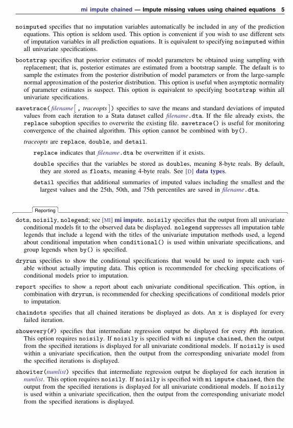
noimputed specifies that no imputation variables automatically be included in any of the predictionequations. This option is seldom used. This option is convenient if you wish to use different setsof imputation variables in all prediction equations. It is equivalent to specifying noimputed withinall univariate specifications.

bootstrap specifies that posterior estimates of model parameters be obtained using sampling withreplacement; that is, posterior estimates are estimated from a bootstrap sample. The default is tosample the estimates from the posterior distribution of model parameters or from the large-samplenormal approximation of the posterior distribution. This option is useful when asymptotic normalityof parameter estimates is suspect. This option is equivalent to specifying bootstrap within allunivariate specifications.

savetrace( filename[, traceopts

]) specifies to save the means and standard deviations of imputed

values from each iteration to a Stata dataset called filename.dta. If the file already exists, thereplace suboption specifies to overwrite the existing file. savetrace() is useful for monitoringconvergence of the chained algorithm. This option cannot be combined with by().

traceopts are replace, double, and detail.

replace indicates that filename.dta be overwritten if it exists.

double specifies that the variables be stored as doubles, meaning 8-byte reals. By default,they are stored as floats, meaning 4-byte reals. See [D] data types.

detail specifies that additional summaries of imputed values including the smallest and thelargest values and the 25th, 50th, and 75th percentiles are saved in filename.dta.

� � �Reporting �

dots, noisily, nolegend; see [MI] mi impute. noisily specifies that the output from all univariateconditional models fit to the observed data be displayed. nolegend suppresses all imputation tablelegends that include a legend with the titles of the univariate imputation methods used, a legendabout conditional imputation when conditional() is used within univariate specifications, andgroup legends when by() is specified.

dryrun specifies to show the conditional specifications that would be used to impute each vari-able without actually imputing data. This option is recommended for checking specifications ofconditional models prior to imputation.

report specifies to show a report about each univariate conditional specification. This option, incombination with dryrun, is recommended for checking specifications of conditional models priorto imputation.

chaindots specifies that all chained iterations be displayed as dots. An x is displayed for everyfailed iteration.

showevery(#) specifies that intermediate regression output be displayed for every #th iteration.This option requires noisily. If noisily is specified with mi impute chained, then the outputfrom the specified iterations is displayed for all univariate conditional models. If noisily is usedwithin a univariate specification, then the output from the corresponding univariate model fromthe specified iterations is displayed.

showiter(numlist) specifies that intermediate regression output be displayed for each iteration innumlist. This option requires noisily. If noisily is specified with mi impute chained, then theoutput from the specified iterations is displayed for all univariate conditional models. If noisilyis used within a univariate specification, then the output from the corresponding univariate modelfrom the specified iterations is displayed.

6 mi impute chained — Impute missing values using chained equations

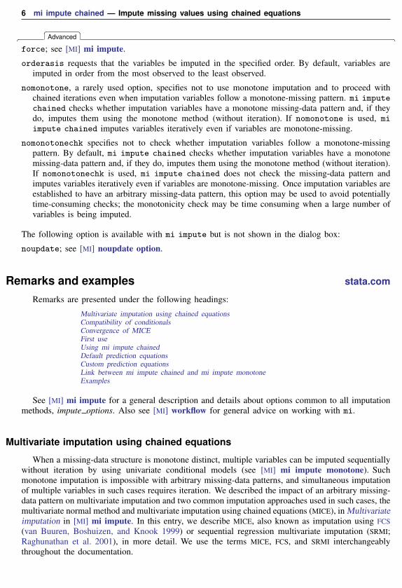
� � �Advanced �

force; see [MI] mi impute.

orderasis requests that the variables be imputed in the specified order. By default, variables areimputed in order from the most observed to the least observed.

nomonotone, a rarely used option, specifies not to use monotone imputation and to proceed withchained iterations even when imputation variables follow a monotone-missing pattern. mi imputechained checks whether imputation variables have a monotone missing-data pattern and, if theydo, imputes them using the monotone method (without iteration). If nomonotone is used, miimpute chained imputes variables iteratively even if variables are monotone-missing.

nomonotonechk specifies not to check whether imputation variables follow a monotone-missingpattern. By default, mi impute chained checks whether imputation variables have a monotonemissing-data pattern and, if they do, imputes them using the monotone method (without iteration).If nomonotonechk is used, mi impute chained does not check the missing-data pattern andimputes variables iteratively even if variables are monotone-missing. Once imputation variables areestablished to have an arbitrary missing-data pattern, this option may be used to avoid potentiallytime-consuming checks; the monotonicity check may be time consuming when a large number ofvariables is being imputed.

The following option is available with mi impute but is not shown in the dialog box:

noupdate; see [MI] noupdate option.

Remarks and examples stata.com

Remarks are presented under the following headings:

Multivariate imputation using chained equationsCompatibility of conditionalsConvergence of MICEFirst useUsing mi impute chainedDefault prediction equationsCustom prediction equationsLink between mi impute chained and mi impute monotoneExamples

See [MI] mi impute for a general description and details about options common to all imputationmethods, impute options. Also see [MI] workflow for general advice on working with mi.

Multivariate imputation using chained equations

When a missing-data structure is monotone distinct, multiple variables can be imputed sequentiallywithout iteration by using univariate conditional models (see [MI] mi impute monotone). Suchmonotone imputation is impossible with arbitrary missing-data patterns, and simultaneous imputationof multiple variables in such cases requires iteration. We described the impact of an arbitrary missing-data pattern on multivariate imputation and two common imputation approaches used in such cases, themultivariate normal method and multivariate imputation using chained equations (MICE), in Multivariateimputation in [MI] mi impute. In this entry, we describe MICE, also known as imputation using FCS(van Buuren, Boshuizen, and Knook 1999) or sequential regression multivariate imputation (SRMI;Raghunathan et al. 2001), in more detail. We use the terms MICE, FCS, and SRMI interchangeablythroughout the documentation.

mi impute chained — Impute missing values using chained equations 7

MICE is similar to monotone imputation in the sense that it is also based on a series of univariateimputation models. Unlike monotone imputation, MICE uses FCSs of prediction equations (chainedequations) and requires iteration. Iteration is needed to account for possible dependence of the estimatedmodel parameters on the imputed data when a missing-data structure is not monotone distinct.

The general idea behind MICE is to impute multiple variables iteratively via a sequence of univariateimputation models, one for each imputation variable, with fully conditional specifications of predictionequations: all variables except the one being imputed are included in a prediction equation. Formally,for imputation variables X1, X2, . . . , Xp and complete predictors (independent variables) Z, thisprocedure can be described as follows. Imputed values are drawn from

X(t+1)1 ∼ g1(X1|X(t)

2 , . . . , X(t)p ,Z,φ1)

X(t+1)2 ∼ g2(X2|X(t+1)

1 , X(t)3 , . . . , X(t)

p ,Z,φ2)

. . .

X(t+1)p ∼ gp(Xp|X(t+1)

1 , X(t+1)2 , . . . , X

(t+1)p−1 ,Z,φp)

(1)

for iterations t = 0, 1, . . . , T until convergence at t = T , where φj are the corresponding modelparameters with a uniform prior. The univariate imputation models, gj(·), can each be of a differenttype (normal, logistic, etc.), as is appropriate for imputing Xj .

Fully conditional specifications (1) are similar to the Gibbs sampling algorithm (Geman andGeman 1984; Gelfand and Smith 1990), one of the MCMC methods for simulating from complicatedmultivariate distributions. In fact, in certain cases these specifications do correspond to a genuine Gibbssampler. For example, when all Xjs are continuous and all gj(·)s are normal linear regressions withconstant variances, then (1) corresponds to a Gibbs sampler based on a multivariate normal distributionwith a uniform prior for model parameters. Such correspondence does not hold in general becauseunlike the Gibbs sampler, the conditional densities {gj(·), j = 1, 2, . . . , p} may not correspondto any multivariate joint conditional distribution of X1, X2, . . . , Xp given Z (Arnold, Castillo, andSarabia 2001). This issue is known as incompatibility of conditionals (for example, Arnold, Castillo,and Sarabia [1999]). When conditionals are not compatible, the MICE procedure may not convergeto any stationary distribution, which can raise concerns about its validity as a principled statisticalmethod; see Compatibility of conditionals and Convergence of MICE for more details.

Despite the lack of a general theoretical justification, MICE is very popular in practice. Its popularityis mainly due to the tremendous flexibility it offers for imputing various types of data arising inobservational studies. Similarly to monotone imputation, the variable-by-variable specification of MICEallows practitioners to simultaneously impute variables of different types by choosing from severalunivariate imputation methods appropriate for each variable. Being able to specify a separate modelfor each variable provides an imputer with great flexibility in incorporating certain characteristicsspecific to each variable. For example, we can use predictive mean matching ([MI] mi impute pmm)or truncated regression ([MI] mi impute truncreg) to impute a variable with a restricted range. Wecan impute variables defined on a subsample using only observations in that subsample while using theentire sample to impute other variables; see Conditional imputation in [MI] mi impute for details. Formore information about multivariate imputation using chained equations, see van Buuren, Boshuizen,and Knook (1999); Raghunathan et al. (2001); van Buuren et al. (2006); van Buuren (2007); White,Royston, and Wood (2011); and Royston (2004, 2005a, 2005b, 2007, 2009), among others.

The specification of a conditional imputation model gj(·) includes an imputation method and aprediction equation relating an imputation variable to other explanatory variables. In what follows,we distinguish between the default specification (of prediction equations) in which the identitiesof the complete explanatory variables are the same across all prediction equations, and the customspecification in which the identities are allowed to differ.

8 mi impute chained — Impute missing values using chained equations

Under the default specification, prediction equations of each imputation variable include all completeindependent variables and all imputation variables except the one being imputed. Under the customspecification, each prediction equation may include a subset of the predictors that would be used underthe default specification. The custom specification also allows expressions of imputation variables inprediction equations.

Model (1) corresponds to the default specification. For example, consider imputation variablesX1, X2, and X3 and complete predictors Z1 and Z2. Under the default specification, the individualprediction equations are determined as follows. The most observed variable—say, X1—is predictedfrom X2, X3, Z1, and Z2. The next most observed variable—say, X2—is predicted from X3, Z1,Z2, and previously imputed X1. The least observed variable, X3, is predicted from Z1, Z2, andpreviously imputed X1 and X2. (A constant is included in all prediction equations, by default.) Weuse the following notation to refer to the above sequence of prediction equations (imputation sequence):X1|X−1, Z1, Z2 → X2|X−2, Z1, Z2 → X3|X−3, Z1, Z2, where X−j denotes all imputed or to-be-imputed variables except Xj .

A sequence such as X1|X−1, Z1 → X2|X−2, Z1, Z2 → X3|X−3, Z2 would correspond to acustom specification. Here X1 is assumed to be conditionally independent of Z2 given X−1 and Z1,and X3 is assumed to be conditionally independent of Z1 given X−3 and Z2.

Compatibility of conditionals

A concern with MICE is its lack of a formal theoretical justification. Its theoretical weakness ispossible incompatibility of fully conditional specifications (1). As we briefly mentioned earlier, it ispossible to specify a set of full conditionals with MICE for which no multivariate distribution exists(for example, van Buuren et al. [2006] and van Buuren [2007]). In such a case, the validity of MICEas a statistical procedure is questionable.

The impact of incompatibility of conditional specifications in practice is still under investigation.For example, van Buuren et al. (2006) performed several simulations to investigate the consequencesof strongly incompatible specifications on multiple-imputation (MI) results in a simple setting andfound very little impact of it on estimated parameters. The effect of incompatible conditionals on thequality of imputations and final MI inference in general is not yet known. Of course, if a joint modelis of main scientific interest, then incompatibility of conditionals poses a problem. In the discussionof Arnold, Castillo, and Sarabia (2001), Andrew Gelman and Trivellore Raghunathan mention thatthe existence of an underlying joint distribution may be less important within the imputation contextthan the ability to incorporate the unique features of the data.

For more information about the compatibility of conditional specifications, see Arnold, Castillo,and Sarabia (2001); van Buuren (2007); and Arnold, Castillo, and Sarabia (1999) and referencestherein.

Convergence of MICE

MICE is an iterative method and is similar in spirit to the Gibbs sampler, an MCMC method.Similarly to MCMC methods, MICE builds a sequence of draws {X(t)

m : t = 1, 2, . . .}, a chain, anditerates until this chain reaches a stationary distribution. So as with any MCMC method, monitoringconvergence is important with MICE.

MICE performs simulation by running multiple independent chains (see Convergence of iterativemethods in [MI] mi impute). To assess convergence of multiple chains, we need to examine thestationarity of each chain by the end of the specified burn-in period b. In practice, convergenceof MICE is often examined visually. Trace plots—plots of summaries of the distribution (means,

mi impute chained — Impute missing values using chained equations 9

standard deviations, quantiles, etc.) of imputed values against iteration numbers—are used to examinestationarity of the chain. Long-term trends in trace plots are indicative of slow convergence tostationarity. A suitable value for the burn-in period b can be inferred from a trace plot as the earliestiteration after which each chain does not exhibit a visible trend and the fluctuations in values becomemore regular. When the initial values are close to the mode of the target posterior distribution (whenone exists), b will generally be small. When the initial values are far off in the tails of the posteriordistribution, the initial number of iterations b will generally be larger.

The number of iterations necessary for MICE to converge depends on, among other things, thefractions of missing information and initial values. The higher the fractions of missing information andthe farther the initial values are from the mode of the posterior predictive distribution of missing data,the slower the convergence, and thus the larger the number of iterations required. Current literaturesuggests that in many practical applications a low number of burn-in iterations, somewhere between5 and 20 iterations, is usually sufficient for convergence (for example, van Buuren [2007]). In anycase, examination of the data and missing-data patterns is highly recommended when investigatingconvergence of MICE.

The convergence of MICE may not be achieved when specified conditional models are incompatible,as described in Compatibility of conditionals. The simulation draws will depend on the order in whichvariables are imputed and on the chosen length of the burn-in period. It is important to evaluate thequality of imputations (see Imputation diagnostics in [MI] mi impute) to determine the impact ofincompatibility on MI analysis.

First useBefore we describe various uses of mi impute chained, let’s look at a simple example first.

Consider the heart attack data example examining the relationship between heart attacks andsmoking from Multivariate imputation of [MI] mi impute, where the age and bmi variables containmissing values. In another version of the dataset, bmi and age have a nonmonotone missing-datapattern, and thus monotone imputation is not possible:

. use http://www.stata-press.com/data/r13/mheart8s0(Fictional heart attack data; arbitrary pattern)

. mi misstable patterns, frequency

Missing-value patterns(1 means complete)

PatternFrequency 1 2

118 1 1

24 1 08 0 14 0 0

154

Variables are (1) age (2) bmi

mi impute chained does not require missing data to be monotone, so we can use it to imputemissing values of age and bmi in this dataset. We use the same model specification as before:

10 mi impute chained — Impute missing values using chained equations

. mi impute chained (regress) bmi age = attack smokes hsgrad female, add(10)

Conditional models:age: regress age bmi attack smokes hsgrad femalebmi: regress bmi age attack smokes hsgrad female

Performing chained iterations ...

Multivariate imputation Imputations = 10Chained equations added = 10Imputed: m=1 through m=10 updated = 0

Initialization: monotone Iterations = 100burn-in = 10

bmi: linear regressionage: linear regression

Observations per m

Variable Complete Incomplete Imputed Total

bmi 126 28 28 154age 142 12 12 154

(complete + incomplete = total; imputed is the minimum across mof the number of filled-in observations.)

As before, 10 imputations are created (the add(10) option). The linear regression imputation method(regress) is used to impute both continuous variables. The attack, smokes, hsgrad, and femalevariables are used as complete predictors (independent variables).

mi impute chained reports the conditional specifications used to impute each variable and theorder in which they were imputed. By default, mi impute chained imputes variables in order fromthe most observed to the least observed. In our example, age has the least number of missing valuesand so is imputed first, even though we listed bmi before age in the command specification.

With the default specification, mi impute chained builds appropriate FCSs automatically usingthe supplied imputation variables and complete predictors, specified as right-hand-side variables. Thedefault prediction equation for age includes bmi and all the complete predictors, and the defaultprediction equation for bmi includes age and all the complete predictors.

The main header and table output were described in detail in [MI] mi impute. The informationspecific to mi impute chained includes the type of initialization, the burn-in period, and the numberof iterations. By default, mi impute chained uses 10 burn-in iterations (also referred to as cycles inthe literature) before drawing imputed values. The total number of iterations performed by mi imputechained to obtain 10 imputations is 100. Also, similarly to mi impute monotone, the additionalinformation above the table includes the legend describing what univariate imputation method wasused to impute each variable. (If desired, this legend may be suppressed by specifying the nolegendoption.)

Using mi impute chained

Below we summarize general capabilities of mi impute chained.

1. mi impute chained offers two main syntaxes—one using the default prediction equationsand the other allowing customization of prediction equations. We will refer to the twosyntaxes as default and custom, respectively. We describe the two syntaxes in detail in thenext two sections.

mi impute chained — Impute missing values using chained equations 11

2. mi impute chained allows specification of a global (outer) if condition,

. mi impute chained . . . if exp . . .

and equation-specific (inner) if conditions,

. mi impute chained . . . (. . . if exp . . . ) . . .

A global if is applied to all equations. You may combine global and equation-specific ifconditions:

. mi impute chained . . . (. . . if exp . . . ) . . . if exp . . .

3. mi impute chained allows specification of global weights, which are applied to all equations:

. mi impute chained . . . [weight] . . .

4. mi impute chained uses fully specified prediction equations by default. Customize predictionequations by including or omitting desired terms:

. mi imp chain (. . . , include(z3) . . . ) (. . . , omit(z1) . . . ) . . .

5. mi impute chained automatically includes appropriate imputation variables in predictionequations. Use a global noimputed option to prevent inclusion of imputation variables inall prediction equations:

. mi impute chained . . . , noimputed . . .

Or use an equation-specific noimputed option to prevent inclusion of imputation variablesin only some prediction equations:

. mi impute chained . . . (. . . , noimputed . . . ) . . .

As we mentioned earlier, mi impute chained is an iterative imputation method. By default, itperforms 10 burn-in iterations for each imputation before drawing the final set of imputed values.The number of iterations is determined by the length of the burn-in period after which a randomsequence (chain) is assumed to converge to its stationary distribution. The provided default may notbe applicable to all situations, so you can use the burnin() option to modify it.

Use the chainonly and savetrace() options to determine the appropriate burn-in period. Forexample,

. mi impute chained . . . , burnin(100) chainonly savetrace(impstats) . . .

saves summaries of imputed values from 100 iterations for each of the imputation variables toimpstats.dta without proceeding to impute data. You can apply techniques from Convergence ofMICE to the data in impstats.dta to determine an adequate burn-in period.

Use a combination of the dryrun and report options to check the specification of each univariateimputation model prior to imputing data.

In the next two sections, we describe the use of mi impute chained first using hypotheticalsituations and then using real examples.

Default prediction equations

We showed in First use an example of mi impute chained with default prediction equationsusing the heart attack data. Here we provide more details about this default specification.

12 mi impute chained — Impute missing values using chained equations

By default, mi impute chained imputes missing values by using the default prediction equations.It builds the corresponding univariate imputation models based on the supplied information: uvmethod,the imputation method; ivars, the imputation variables; and indepvars, the complete predictors orindependent variables.

Suppose that continuous variables x1, x2, and x3 contain missing values and are ordered from themost observed to the least observed. We want to impute these variables, and we decide to use thesame univariate imputation method, say, linear regression, for all. We can do this by typing

. mi impute chained (regress) x1 x2 x3 . . .

The above command corresponds to the first syntax diagram of mi impute chained: uvmethodis regress and ivars is x1 x2 x3. Relating the above to the model notation used in (1), g1, g2,g3 represent linear regression imputation models and the prediction sequence is X1|X2, X3 →X2|X1, X3 → X3|X1, X2.

By default, mi impute chained imputes variables in order from the most observed to the leastobserved, regardless of the order in which variables were specified. For example, we can list imputationvariables in the reverse order,

. mi impute chained (regress) x3 x2 x1 . . .

and mi impute chained will still impute x1 first, x2 second, and x3 last. You can use the orderasisoption to instruct mi impute chained to perform imputation of variables in the specified order.

If we have additional covariates containing no missing values (say, z1 and z2) that we want toinclude in the imputation model, we can do so by typing

. mi impute chained (regress) x1 x2 x3 = z1 z2 . . .

Now indepvars is z1 z2 and the prediction sequence is X1|X2, X3, Z1, Z2 → X2|X1, X3, Z1, Z2 →X3|X1, X2, Z1, Z2. Independent variables are included in the prediction equations of all univariatemodels.

Suppose that we want to use a different imputation method for one of the variables—we want toimpute x3 using predictive mean matching. We can do this by typing

. mi impute chained (regress) x1 x2 (pmm) x3 = z1 z2 . . .

The above corresponds to the second syntax diagram of mi impute chained, a generalization ofthe first that accommodates differing imputation methods. The right-hand side of the equation isunchanged. z1 and z2 are included in all three prediction equations. The left-hand side now has twospecifications: (regress) x1 x2 and (pmm) x3. In previous examples, we had only one left-hand-sidespecification, lhs spec—(regress) x1 x2 x3. (The number of left-hand-side specifications does notnecessarily correspond to the number of univariate models; the latter is determined by the numberof imputation variables.) In this example, x1 and x2 are imputed using linear regression, and x3 isimputed using predictive mean matching.

Now, instead of using the default one nearest neighbor with pmm, say that we want to use three, whichrequires pmm’s knn(3) option. All method-specific options must be specified within the parenthesessurrounding the method:

. mi impute chained (regress) x1 x2 (pmm, knn(3)) x3 = z1 z2 . . .

Suppose now we want to restrict the imputation sample for x2 to observations where z1 is one;also see Imputing on subsamples of [MI] mi impute. (We also omit pmm’s knn() option here.) Thecorresponding syntax is

. mi impute chained (regress) x1 (regress if z1==1) x2 (pmm) x3 = z1 z2 . . .

mi impute chained — Impute missing values using chained equations 13

If, in addition to the above, we want to impute all variables using an overall subsample where z3is one, we can specify the global if z3==1 condition:

. mi impute chained (regress) x1 (regress if z1==1) x2 (pmm) x3 = z1 z2> if z3==1 . . .

In the above, restrictions included only complete variables. When restrictions include imputationvariables, you should use the conditional() option instead of an if condition; see Conditionalimputation in [MI] mi impute. Suppose that we need to impute x2 using only observations for whichx1 is positive, provided that missing values of x1 are nested within missing values of x2. We can dothis by typing

. mi impute chained (regress) x1 (regress, cond(if x1>0)) x2 (pmm) x3 = z1 z2 . . .

When any imputation variable is imputed using a categorical method, mi impute chainedautomatically includes it as a factor variable in the prediction equations of other imputation variables.Suppose that x1 is a categorical variable and is imputed using the multinomial logistic method:

. mi impute chained (mlogit) x1 (regress) x2 x3 . . .

The above will result in the prediction sequence X1|X2, X3 → X2|i.X1, X3 → X3|i.X1, X2

where i.X1 denotes the factors of X1.

If you wish to include a factor variable as continuous in prediction equations, you can use theascontinuous option within the specification of the univariate imputation method for that variable:

. mi impute chained (mlogit, ascontinuous) x1 (regress) x2 x3 . . .

As we discussed in The issue of perfect prediction during imputation of categorical data of [MI] miimpute, perfect prediction often occurs during imputation of categorical variables. One way of dealingwith it is to use the augmented-regression approach (White, Daniel, and Royston 2010), availablethrough the augment option. For example, if perfect prediction occurs during imputation of x1 inthe above, you can specify augment within the method specification of x1 to perform augmentedregression:

. mi impute chained (mlogit, augment) x1 (regress) x2 x3 . . .

Alternatively, you can use the augment option with mi impute chained to perform augmentedregression for all categorical variables for which the issue of perfect prediction arises:

. mi impute chained (mlogit) x1 (logit) x2 (regress) x3 . . . , augment . . .

The above is equivalent to specifying augment within each specification of a univariate categoricalimputation method:

. mi impute chained (mlogit, augment) x1 (logit, augment) x2 (regress) x3 . . .

Custom prediction equations

In the previous section, we considered various uses of mi impute chained with default predictionequations. Often, however, you may want to use different prediction equations for some or even allimputation variables. We can easily modify the above specifications to accommodate this.

Let’s consider situations in which we want to use different sets of complete variables for someimputation variables first. Recall our following hypothetical example:

. mi impute chained (regress) x1 x2 x3 = z1 z2 . . . (M1)

14 mi impute chained — Impute missing values using chained equations

Suppose that we want to omit z2 from the prediction equation for x3. To accommodate this, weneed to include two separate specifications: one for x1 and x2 and one for x3:

. mi impute chained (regress) x1 x2 (regress, omit(z2)) x3 = z1 z2 . . .

The above corresponds to the custom specification, the third syntax diagram, of mi imputechained. As before, we list all the complete variables indepvars to be included in all predictionequations to the right of the = sign. So, indepvars is still z1 z2. The prediction equation for x3,however, omits variable z2, specified within the omit() option. The prediction sequence for theabove specification is X1|X2, X3, Z1, Z2 → X2|X1, X3, Z1, Z2 → X3|X1, X2, Z1.

Alternatively, we could have achieved the above by including variable z1 in all prediction equations,as a right-hand-side specification indepvars, and using the include() option to add variable z2 tothe prediction equations of x1 and x2:

. mi impute chained (regress, include(z2)) x1 x2 (regress) x3 = z1 . . .

You may also want to modify the sets of imputation variables to be included in prediction equations.By default, mi impute chained automatically includes the appropriate fully conditional specificationsof imputation variables in all prediction equations.

Suppose that in addition to different sets of complete predictors, we assume that X1 and X2 areconditionally independent given X3, which implies that prediction equations for x1 and x2 includeonly x3 and not each other. We can accommodate this with the command

. mi impute chained (regress, include(x3 z2) noimputed) x1 x2 (regress) ///x3 = z1 . . .

which corresponds to the prediction sequence X1|X3, Z1, Z2 → X2|X3, Z1, Z2 → X3|X1, X2, Z1.

The above is also equivalent to the command

. mi impute chained (regress, omit(x1 x2)) x1 x2 (regress, omit(z2)) ///x3 = z1 z2 . . .

There are other equivalent ways of achieving the above custom specifications by using variouscombinations of include(), omit(), and noimputed. The most convenient specification will dependon your particular structure of the prediction equations. You can also combine these options withinthe same univariate specification.

It is important to realize that equivalent syntaxes may produce different (yet equivalent withstable imputation models) sequences of imputed values when they have different ordering of variablesin prediction equations. mi impute chained builds prediction equations as follows. Appropriateimputation variables are included first, unless the noimputed option is specified. By default, imputationvariables are included in order from the most observed to the least observed. If the orderasis optionis used, the variables are included in the specified order. Next, terms specified in the include()option are included in the listed order. Then right-hand-side variables (indepvars) are included in thelisted order. Finally, variables listed in the omit() option are removed from the prediction equation.When you specify omit(), it is important to specify variables as they are included in the predictionequation; if x1 is included as a factor variable, omit(i.x1) should be used.

You can also include functions of imputation variables in prediction equations with the customspecification of mi impute chained. As we discussed in Model building in [MI] mi impute, thereare two ways to do that. You can include functions of imputation variables as separate imputationvariables directly in your imputation model or you can impute them passively using mi imputechained.

mi impute chained — Impute missing values using chained equations 15

For example, using model (M1), suppose that we would like to include the interaction betweenx1 and x2 in the conditional model for x3:

. mi impute chained (regress) x1 x2 ///(regress, include((x1*x2))) x3 ///

= z1 z2 . . .

The expression x1*x2, specified in the include() option, is enclosed in parentheses.

We also could have typed

. mi impute chained (regress, include((x1*x2))) x1 x2 x3 = z1 z2 . . .

and mi impute chained would appropriately include the interaction term X1X2 only in the predictionequation of X3.

You can include any other expressions of imputation variables in include() within any of theleft-hand-side specifications. Just remember to enclose such expressions in parentheses.

All the examples we considered in Default prediction equations are also applicable to mi imputechained with custom prediction equations. For example, to restrict imputation of x2 to observationswhere z1==1 in one of our earlier examples, we can type

. mi impute chained (reg) x1 (reg if z1==1) x2 (reg, omit(z2)) x3 = z1 z2 . . .

Link between mi impute chained and mi impute monotone

Similarly to mi impute monotone (see [MI] mi impute monotone), mi impute chained uses asequence of univariate imputation models to impute variables. So the use of mi impute chained isvery similar to that of mi impute monotone except:

1. mi impute chained does not require that the specified imputation variables follow amonotone-missing pattern.

2. mi impute chained requires iteration to accommodate arbitrary missing-data patterns.

3. mi impute chained, by default, uses FCSs of the prediction equations where all specifiedcomplete variables and all imputation variables except the one being imputed are includedin prediction equations.

4. mi impute chained provides an alternative way of specifying custom prediction equationsto accommodate FCS of imputation variables.

When a missing-value pattern is monotone, mi impute chained defaults to the monotone method(unless nomonotone is specified) and produces the same results as mi impute monotone. However,using mi impute monotone in this case is faster because it performs the estimation step only once,on the original data, whereas mi impute chained performs estimation on every chained iteration.

The best approach to follow is

1. Check the missing-data pattern using misstable nested (or mi misstable nested if thedata are already mi set; see [R] misstable or [MI] mi misstable) first.

2. If the missing-data pattern is monotone, use mi impute monotone to impute variables. Ifthe missing-data pattern is not monotone, use mi impute chained to impute variables.

It is worth mentioning the difference between the documented custom syntaxes of mi imputechained and mi impute monotone.

16 mi impute chained — Impute missing values using chained equations

With monotone imputation, variables are imputed in a particular, monotone-missing order andprediction equations are built in a particular way: previously imputed variables are added sequentially tothe prediction equations of other imputation variables. So when building custom prediction equations,it is easier to construct one equation at a time in the order of the monotone missing pattern. As such,the custom syntax of mi impute monotone, as documented in [MI] mi impute monotone, requiresfull specification of a separate conditional model for each imputation variable in the monotone-missingorder.

Imputation using chained equations does not require specific ordering in which variables must beimputed, although imputing variables in order from the most observed to the least observed usuallyleads to faster convergence. Also, because all imputation variables except the one being imputed areincluded in prediction equations, it does not matter in what order prediction equations are specified.The custom syntax of mi impute chained reflects this.

Examples

For the purpose of illustration, we use five imputations in our examples.

Example 1: Different imputation methods

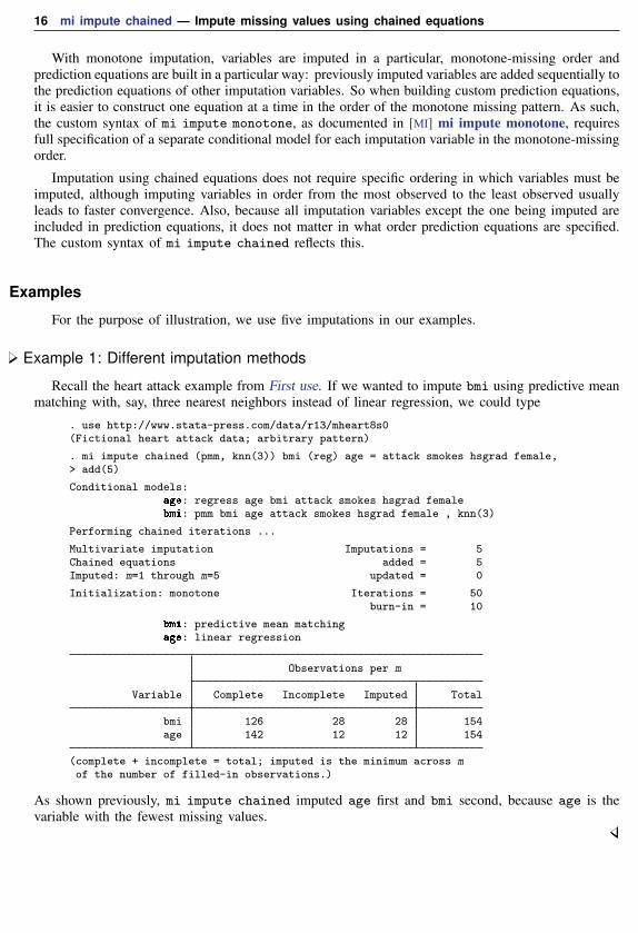
Recall the heart attack example from First use. If we wanted to impute bmi using predictive meanmatching with, say, three nearest neighbors instead of linear regression, we could type

. use http://www.stata-press.com/data/r13/mheart8s0(Fictional heart attack data; arbitrary pattern)

. mi impute chained (pmm, knn(3)) bmi (reg) age = attack smokes hsgrad female,> add(5)

Conditional models:age: regress age bmi attack smokes hsgrad femalebmi: pmm bmi age attack smokes hsgrad female , knn(3)

Performing chained iterations ...

Multivariate imputation Imputations = 5Chained equations added = 5Imputed: m=1 through m=5 updated = 0

Initialization: monotone Iterations = 50burn-in = 10

bmi: predictive mean matchingage: linear regression

Observations per m

Variable Complete Incomplete Imputed Total

bmi 126 28 28 154age 142 12 12 154

(complete + incomplete = total; imputed is the minimum across mof the number of filled-in observations.)

As shown previously, mi impute chained imputed age first and bmi second, because age is thevariable with the fewest missing values.

mi impute chained — Impute missing values using chained equations 17

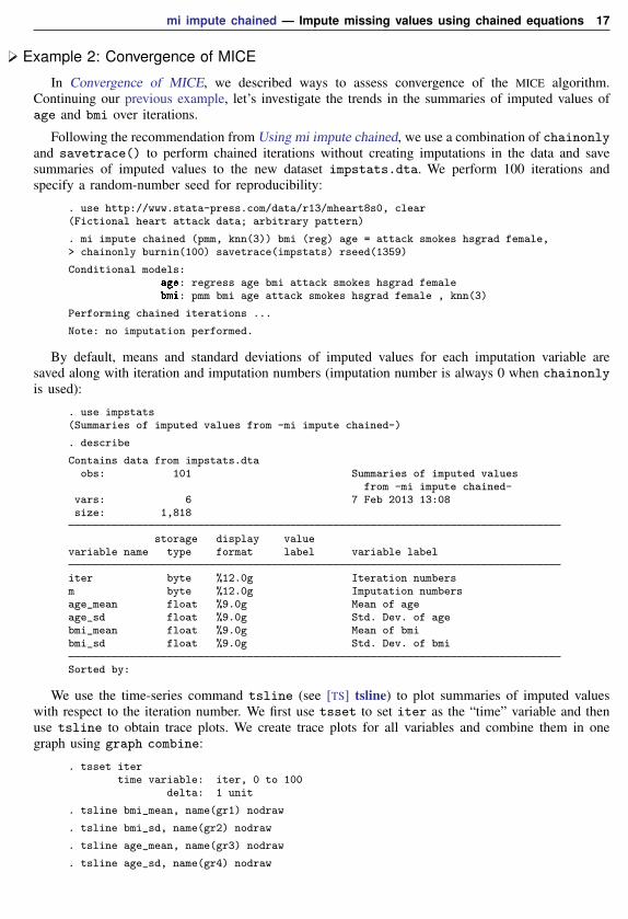
Example 2: Convergence of MICE

In Convergence of MICE, we described ways to assess convergence of the MICE algorithm.Continuing our previous example, let’s investigate the trends in the summaries of imputed values ofage and bmi over iterations.

Following the recommendation from Using mi impute chained, we use a combination of chainonlyand savetrace() to perform chained iterations without creating imputations in the data and savesummaries of imputed values to the new dataset impstats.dta. We perform 100 iterations andspecify a random-number seed for reproducibility:

. use http://www.stata-press.com/data/r13/mheart8s0, clear(Fictional heart attack data; arbitrary pattern)

. mi impute chained (pmm, knn(3)) bmi (reg) age = attack smokes hsgrad female,> chainonly burnin(100) savetrace(impstats) rseed(1359)

Conditional models:age: regress age bmi attack smokes hsgrad femalebmi: pmm bmi age attack smokes hsgrad female , knn(3)

Performing chained iterations ...

Note: no imputation performed.

By default, means and standard deviations of imputed values for each imputation variable aresaved along with iteration and imputation numbers (imputation number is always 0 when chainonlyis used):

. use impstats(Summaries of imputed values from -mi impute chained-)

. describe

Contains data from impstats.dtaobs: 101 Summaries of imputed values

from -mi impute chained-vars: 6 7 Feb 2013 13:08size: 1,818

storage display valuevariable name type format label variable label

iter byte %12.0g Iteration numbersm byte %12.0g Imputation numbersage_mean float %9.0g Mean of ageage_sd float %9.0g Std. Dev. of agebmi_mean float %9.0g Mean of bmibmi_sd float %9.0g Std. Dev. of bmi

Sorted by:

We use the time-series command tsline (see [TS] tsline) to plot summaries of imputed valueswith respect to the iteration number. We first use tsset to set iter as the “time” variable and thenuse tsline to obtain trace plots. We create trace plots for all variables and combine them in onegraph using graph combine:

. tsset itertime variable: iter, 0 to 100

delta: 1 unit

. tsline bmi_mean, name(gr1) nodraw

. tsline bmi_sd, name(gr2) nodraw

. tsline age_mean, name(gr3) nodraw

. tsline age_sd, name(gr4) nodraw

18 mi impute chained — Impute missing values using chained equations

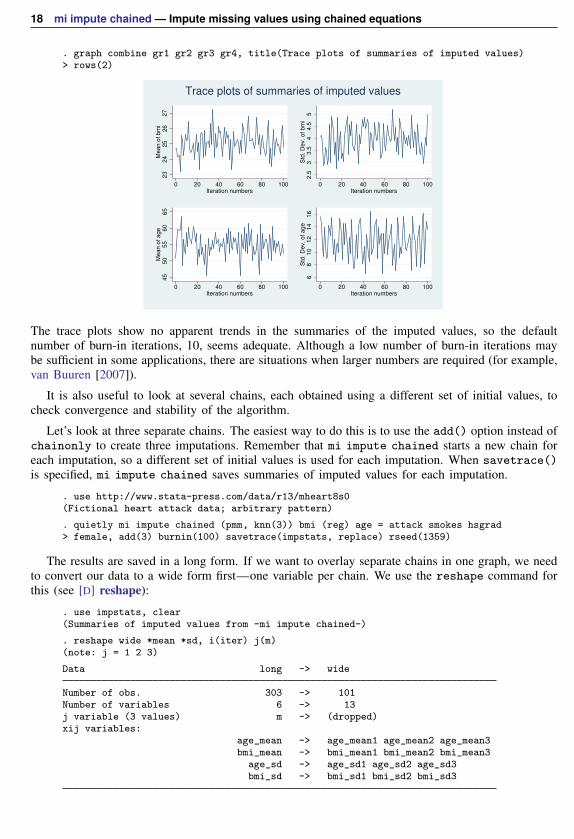
. graph combine gr1 gr2 gr3 gr4, title(Trace plots of summaries of imputed values)> rows(2)

23

24

25

26

27

Me

an

of

bm

i

0 20 40 60 80 100Iteration numbers

2.5

33

.54

4.5

5S

td.

De

v.

of

bm

i

0 20 40 60 80 100Iteration numbers

45

50

55

60

65

Me

an

of

ag

e

0 20 40 60 80 100Iteration numbers

68

10

12

14

16

Std

. D

ev.

of

ag

e

0 20 40 60 80 100Iteration numbers

Trace plots of summaries of imputed values

The trace plots show no apparent trends in the summaries of the imputed values, so the defaultnumber of burn-in iterations, 10, seems adequate. Although a low number of burn-in iterations maybe sufficient in some applications, there are situations when larger numbers are required (for example,van Buuren [2007]).

It is also useful to look at several chains, each obtained using a different set of initial values, tocheck convergence and stability of the algorithm.

Let’s look at three separate chains. The easiest way to do this is to use the add() option instead ofchainonly to create three imputations. Remember that mi impute chained starts a new chain foreach imputation, so a different set of initial values is used for each imputation. When savetrace()is specified, mi impute chained saves summaries of imputed values for each imputation.

. use http://www.stata-press.com/data/r13/mheart8s0(Fictional heart attack data; arbitrary pattern)

. quietly mi impute chained (pmm, knn(3)) bmi (reg) age = attack smokes hsgrad> female, add(3) burnin(100) savetrace(impstats, replace) rseed(1359)

The results are saved in a long form. If we want to overlay separate chains in one graph, we needto convert our data to a wide form first—one variable per chain. We use the reshape command forthis (see [D] reshape):

. use impstats, clear(Summaries of imputed values from -mi impute chained-)

. reshape wide *mean *sd, i(iter) j(m)(note: j = 1 2 3)

Data long -> wide

Number of obs. 303 -> 101Number of variables 6 -> 13j variable (3 values) m -> (dropped)xij variables:

age_mean -> age_mean1 age_mean2 age_mean3bmi_mean -> bmi_mean1 bmi_mean2 bmi_mean3

age_sd -> age_sd1 age_sd2 age_sd3bmi_sd -> bmi_sd1 bmi_sd2 bmi_sd3

mi impute chained — Impute missing values using chained equations 19

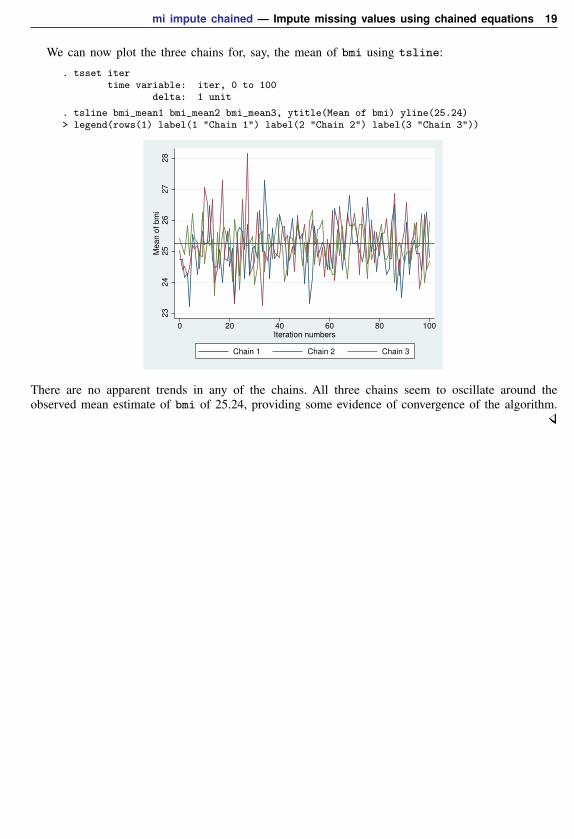
We can now plot the three chains for, say, the mean of bmi using tsline:

. tsset itertime variable: iter, 0 to 100

delta: 1 unit

. tsline bmi_mean1 bmi_mean2 bmi_mean3, ytitle(Mean of bmi) yline(25.24)> legend(rows(1) label(1 "Chain 1") label(2 "Chain 2") label(3 "Chain 3"))

23

24

25

26

27

28

Me

an

of

bm

i

0 20 40 60 80 100

Iteration numbers

Chain 1 Chain 2 Chain 3

There are no apparent trends in any of the chains. All three chains seem to oscillate around theobserved mean estimate of bmi of 25.24, providing some evidence of convergence of the algorithm.

20 mi impute chained — Impute missing values using chained equations

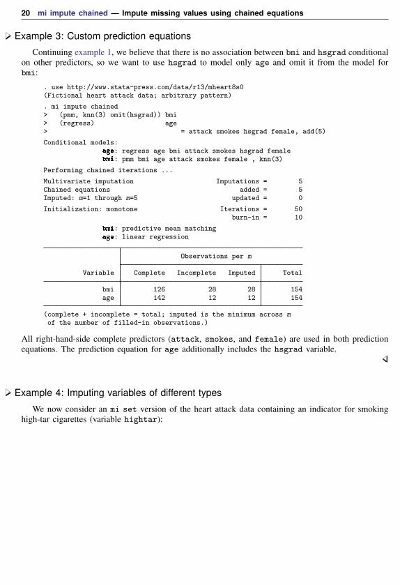
Example 3: Custom prediction equations

Continuing example 1, we believe that there is no association between bmi and hsgrad conditionalon other predictors, so we want to use hsgrad to model only age and omit it from the model forbmi:

. use http://www.stata-press.com/data/r13/mheart8s0(Fictional heart attack data; arbitrary pattern)

. mi impute chained> (pmm, knn(3) omit(hsgrad)) bmi> (regress) age> = attack smokes hsgrad female, add(5)

Conditional models:age: regress age bmi attack smokes hsgrad femalebmi: pmm bmi age attack smokes female , knn(3)

Performing chained iterations ...

Multivariate imputation Imputations = 5Chained equations added = 5Imputed: m=1 through m=5 updated = 0

Initialization: monotone Iterations = 50burn-in = 10

bmi: predictive mean matchingage: linear regression

Observations per m

Variable Complete Incomplete Imputed Total

bmi 126 28 28 154age 142 12 12 154

(complete + incomplete = total; imputed is the minimum across mof the number of filled-in observations.)

All right-hand-side complete predictors (attack, smokes, and female) are used in both predictionequations. The prediction equation for age additionally includes the hsgrad variable.

Example 4: Imputing variables of different types

We now consider an mi set version of the heart attack data containing an indicator for smokinghigh-tar cigarettes (variable hightar):

mi impute chained — Impute missing values using chained equations 21

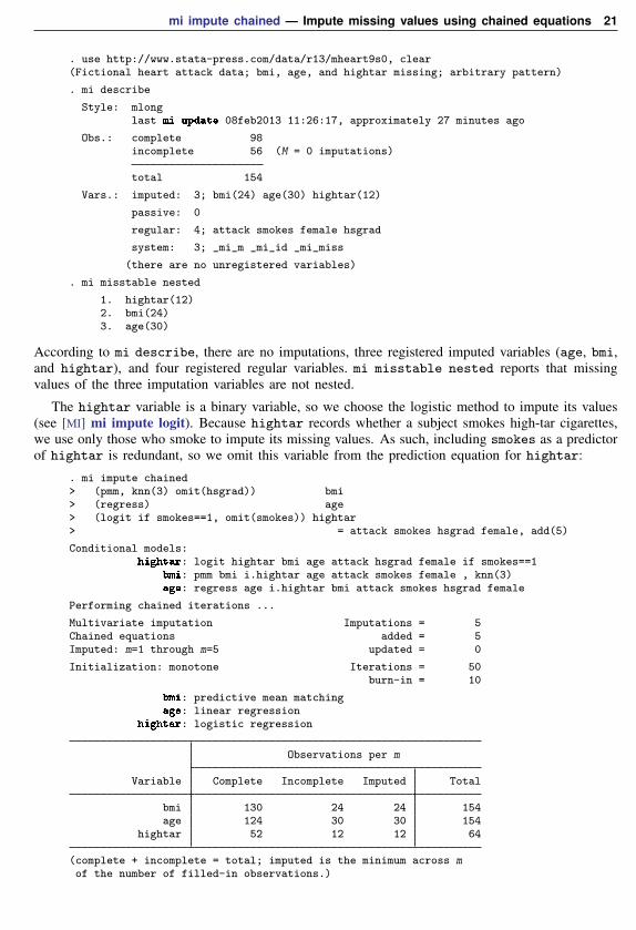
. use http://www.stata-press.com/data/r13/mheart9s0, clear(Fictional heart attack data; bmi, age, and hightar missing; arbitrary pattern)

. mi describe

Style: mlonglast mi update 08feb2013 11:26:17, approximately 27 minutes ago

Obs.: complete 98incomplete 56 (M = 0 imputations)

total 154

Vars.: imputed: 3; bmi(24) age(30) hightar(12)

passive: 0

regular: 4; attack smokes female hsgrad

system: 3; _mi_m _mi_id _mi_miss

(there are no unregistered variables)

. mi misstable nested

1. hightar(12)2. bmi(24)3. age(30)

According to mi describe, there are no imputations, three registered imputed variables (age, bmi,and hightar), and four registered regular variables. mi misstable nested reports that missingvalues of the three imputation variables are not nested.

The hightar variable is a binary variable, so we choose the logistic method to impute its values(see [MI] mi impute logit). Because hightar records whether a subject smokes high-tar cigarettes,we use only those who smoke to impute its missing values. As such, including smokes as a predictorof hightar is redundant, so we omit this variable from the prediction equation for hightar:

. mi impute chained> (pmm, knn(3) omit(hsgrad)) bmi> (regress) age> (logit if smokes==1, omit(smokes)) hightar> = attack smokes hsgrad female, add(5)

Conditional models:hightar: logit hightar bmi age attack hsgrad female if smokes==1

bmi: pmm bmi i.hightar age attack smokes female , knn(3)age: regress age i.hightar bmi attack smokes hsgrad female

Performing chained iterations ...

Multivariate imputation Imputations = 5Chained equations added = 5Imputed: m=1 through m=5 updated = 0

Initialization: monotone Iterations = 50burn-in = 10

bmi: predictive mean matchingage: linear regression

hightar: logistic regression

Observations per m

Variable Complete Incomplete Imputed Total

bmi 130 24 24 154age 124 30 30 154

hightar 52 12 12 64

(complete + incomplete = total; imputed is the minimum across mof the number of filled-in observations.)

22 mi impute chained — Impute missing values using chained equations

From the output, we see that all incomplete values of each of the variables are imputed in allimputations. Because we restricted the imputation sample of hightar to smokers, the total numberof observations reported for hightar is 64 and not 154. mi impute chained also automaticallyincluded the binary variable hightar as a factor variable in prediction equations for age and bmibecause we used logit to impute it.

As we described in Conditional imputation, you should be careful when using an if statementfor imputing variables conditionally on other variables. It was safe to use if here, because smokesdid not contain missing values and there were no missing values of hightar for the subjects whodo not smoke.

Example 5: Conditional imputation

Continuing example 4, suppose now that the smokes variable also contains missing values:

. use http://www.stata-press.com/data/r13/mheart10s0, clear(Fict. heart attack data; bmi, age, hightar, & smokes missing; arbitrary pattern)

. mi describe

Style: mlonglast mi update 08feb2013 11:26:06, approximately 27 minutes ago

Obs.: complete 92incomplete 62 (M = 0 imputations)

total 154

Vars.: imputed: 4; bmi(24) age(30) hightar(19) smokes(14)

passive: 0

regular: 3; attack female hsgrad

system: 3; _mi_m _mi_id _mi_miss

(there are no unregistered variables)

. mi misstable nested

1. smokes(14) -> hightar(19)2. bmi(24)3. age(30)

The smokes variable is now registered as imputed and the three regular variables are now attack,female, and hsgrad. mi misstable nested reports that although the missing-data pattern withrespect to all four imputation variables is not monotone, the missing-data pattern with respect tosmokes and hightar is monotone. Recall from Conditional imputation that one of the requirementsof conditional imputation is that missing values of all conditioning variables (smokes) are nestedwithin missing values of the conditional variable (hightar). So this requirement is satisfied in ourdata.

Because smokes contains missing values, we cannot use an if condition to restrict the imputationsample of hightar to those who smoke. We must use the conditional() option. We use thelogistic method (see [MI] mi impute logit) to fill in missing values of smokes.

mi impute chained — Impute missing values using chained equations 23

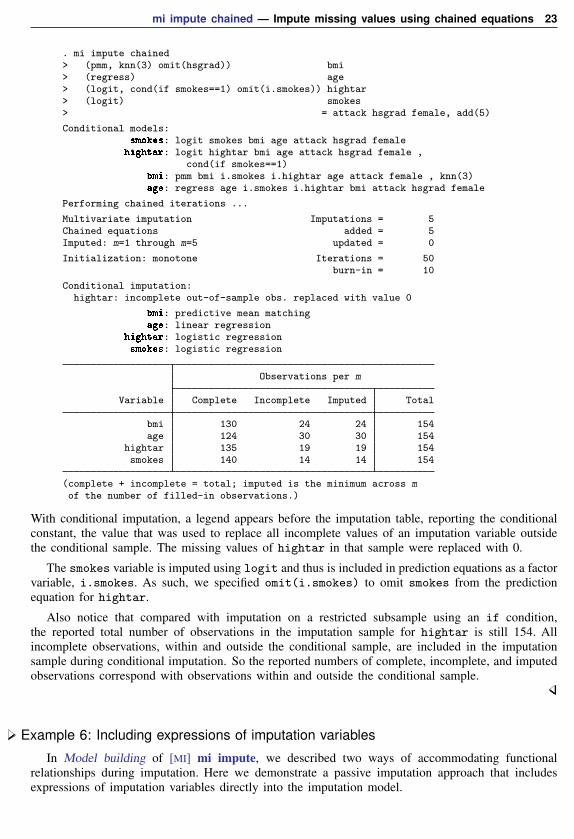
. mi impute chained> (pmm, knn(3) omit(hsgrad)) bmi> (regress) age> (logit, cond(if smokes==1) omit(i.smokes)) hightar> (logit) smokes> = attack hsgrad female, add(5)

Conditional models:smokes: logit smokes bmi age attack hsgrad femalehightar: logit hightar bmi age attack hsgrad female ,

cond(if smokes==1)bmi: pmm bmi i.smokes i.hightar age attack female , knn(3)age: regress age i.smokes i.hightar bmi attack hsgrad female

Performing chained iterations ...

Multivariate imputation Imputations = 5Chained equations added = 5Imputed: m=1 through m=5 updated = 0

Initialization: monotone Iterations = 50burn-in = 10

Conditional imputation:hightar: incomplete out-of-sample obs. replaced with value 0

bmi: predictive mean matchingage: linear regression

hightar: logistic regressionsmokes: logistic regression

Observations per m

Variable Complete Incomplete Imputed Total

bmi 130 24 24 154age 124 30 30 154

hightar 135 19 19 154smokes 140 14 14 154

(complete + incomplete = total; imputed is the minimum across mof the number of filled-in observations.)

With conditional imputation, a legend appears before the imputation table, reporting the conditionalconstant, the value that was used to replace all incomplete values of an imputation variable outsidethe conditional sample. The missing values of hightar in that sample were replaced with 0.

The smokes variable is imputed using logit and thus is included in prediction equations as a factorvariable, i.smokes. As such, we specified omit(i.smokes) to omit smokes from the predictionequation for hightar.

Also notice that compared with imputation on a restricted subsample using an if condition,the reported total number of observations in the imputation sample for hightar is still 154. Allincomplete observations, within and outside the conditional sample, are included in the imputationsample during conditional imputation. So the reported numbers of complete, incomplete, and imputedobservations correspond with observations within and outside the conditional sample.

Example 6: Including expressions of imputation variables

In Model building of [MI] mi impute, we described two ways of accommodating functionalrelationships during imputation. Here we demonstrate a passive imputation approach that includesexpressions of imputation variables directly into the imputation model.

24 mi impute chained — Impute missing values using chained equations

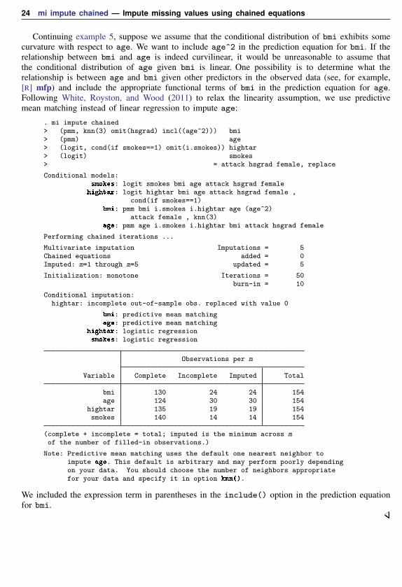
Continuing example 5, suppose we assume that the conditional distribution of bmi exhibits somecurvature with respect to age. We want to include age^2 in the prediction equation for bmi. If therelationship between bmi and age is indeed curvilinear, it would be unreasonable to assume thatthe conditional distribution of age given bmi is linear. One possibility is to determine what therelationship is between age and bmi given other predictors in the observed data (see, for example,[R] mfp) and include the appropriate functional terms of bmi in the prediction equation for age.Following White, Royston, and Wood (2011) to relax the linearity assumption, we use predictivemean matching instead of linear regression to impute age:

. mi impute chained> (pmm, knn(3) omit(hsgrad) incl((age^2))) bmi> (pmm) age> (logit, cond(if smokes==1) omit(i.smokes)) hightar> (logit) smokes> = attack hsgrad female, replace

Conditional models:smokes: logit smokes bmi age attack hsgrad femalehightar: logit hightar bmi age attack hsgrad female ,

cond(if smokes==1)bmi: pmm bmi i.smokes i.hightar age (age^2)

attack female , knn(3)age: pmm age i.smokes i.hightar bmi attack hsgrad female

Performing chained iterations ...

Multivariate imputation Imputations = 5Chained equations added = 0Imputed: m=1 through m=5 updated = 5

Initialization: monotone Iterations = 50burn-in = 10

Conditional imputation:hightar: incomplete out-of-sample obs. replaced with value 0

bmi: predictive mean matchingage: predictive mean matching

hightar: logistic regressionsmokes: logistic regression

Observations per m

Variable Complete Incomplete Imputed Total

bmi 130 24 24 154age 124 30 30 154

hightar 135 19 19 154smokes 140 14 14 154

(complete + incomplete = total; imputed is the minimum across mof the number of filled-in observations.)

Note: Predictive mean matching uses the default one nearest neighbor toimpute age. This default is arbitrary and may perform poorly dependingon your data. You should choose the number of neighbors appropriatefor your data and specify it in option knn().

We included the expression term in parentheses in the include() option in the prediction equationfor bmi.

mi impute chained — Impute missing values using chained equations 25

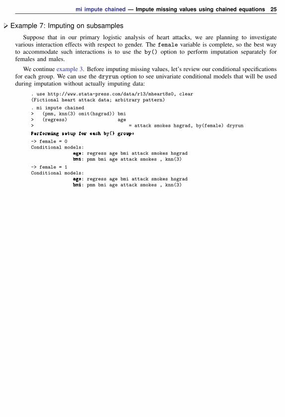
Example 7: Imputing on subsamples

Suppose that in our primary logistic analysis of heart attacks, we are planning to investigatevarious interaction effects with respect to gender. The female variable is complete, so the best wayto accommodate such interactions is to use the by() option to perform imputation separately forfemales and males.

We continue example 3. Before imputing missing values, let’s review our conditional specificationsfor each group. We can use the dryrun option to see univariate conditional models that will be usedduring imputation without actually imputing data:

. use http://www.stata-press.com/data/r13/mheart8s0, clear(Fictional heart attack data; arbitrary pattern)

. mi impute chained> (pmm, knn(3) omit(hsgrad)) bmi> (regress) age> = attack smokes hsgrad, by(female) dryrun

Performing setup for each by() group:

-> female = 0Conditional models:

age: regress age bmi attack smokes hsgradbmi: pmm bmi age attack smokes , knn(3)

-> female = 1Conditional models:

age: regress age bmi attack smokes hsgradbmi: pmm bmi age attack smokes , knn(3)

26 mi impute chained — Impute missing values using chained equations

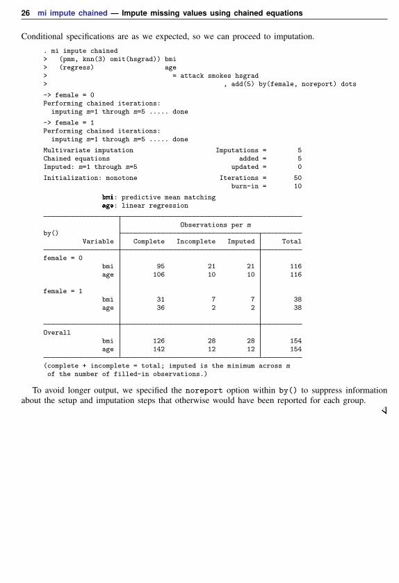
Conditional specifications are as we expected, so we can proceed to imputation.

. mi impute chained> (pmm, knn(3) omit(hsgrad)) bmi> (regress) age> = attack smokes hsgrad> , add(5) by(female, noreport) dots

-> female = 0Performing chained iterations:

imputing m=1 through m=5 ..... done

-> female = 1Performing chained iterations:

imputing m=1 through m=5 ..... done

Multivariate imputation Imputations = 5Chained equations added = 5Imputed: m=1 through m=5 updated = 0

Initialization: monotone Iterations = 50burn-in = 10

bmi: predictive mean matchingage: linear regression

Observations per mby()

Variable Complete Incomplete Imputed Total

female = 0bmi 95 21 21 116age 106 10 10 116

female = 1bmi 31 7 7 38age 36 2 2 38

Overallbmi 126 28 28 154age 142 12 12 154

(complete + incomplete = total; imputed is the minimum across mof the number of filled-in observations.)

To avoid longer output, we specified the noreport option within by() to suppress informationabout the setup and imputation steps that otherwise would have been reported for each group.

mi impute chained — Impute missing values using chained equations 27

Stored resultsmi impute chained stores the following in r():

Scalarsr(M) total number of imputationsr(M add) number of added imputationsr(M update) number of updated imputationsr(k ivars) number of imputed variablesr(burnin) number of burn-in iterationsr(N g) number of imputed groups (1 if by() is not specified)

Macrosr(method) name of imputation method (chained)r(ivars) names of imputation variablesr(uvmethods) names of univariate imputation methodsr(init) type of initializationr(rseed) random-number seedr(by) names of variables specified within by()

Matricesr(N) number of observations in imputation sample in each group (per variable)r(N complete) number of complete observations in imputation sample in each group (per variable)r(N incomplete) number of incomplete observations in imputation sample in each group (per variable)r(N imputed) number of imputed observations in imputation sample in each group (per variable)

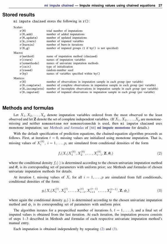
Methods and formulasLet X1, X2, . . . , Xp denote imputation variables ordered from the most observed to the least

observed and let Z denote the set of complete independent variables. (If X1, X2, . . . , Xp are monotone-missing and neither nomonotone nor nomonotonechk is used, then mi impute chained usesmonotone imputation; see Methods and formulas of [MI] mi impute monotone for details.)

With the default specification of prediction equations, the chained-equation algorithm proceeds asfollows. First, at iteration t = 0, missing values are initialized using monotone imputation. That is,missing values of X(0)

i , i = 1, . . . , p, are simulated from conditional densities of the form

fi(Xi|X(0)1 , X

(0)2 , . . . , X

(0)i−1,Z, θi) (2)

where the conditional density fi(·) is determined according to the chosen univariate imputation methodand θi is its corresponding set of parameters with uniform prior; see Methods and formulas of chosenunivariate imputation methods for details.

At iteration t, missing values of Xi for all i = 1, . . . , p are simulated from full conditionals,conditional densities of the form:

gi(Xi|X(t)1 , X

(t)2 , . . . , X

(t)i−1, X

(t−1)i+1 , . . . , X(t−1)

p ,Z,φi) (3)

where again the conditional density gi(·) is determined according to the chosen univariate imputationmethod and φi is its corresponding set of parameters with uniform prior.

The algorithm iterates for a prespecified number of iterations b, t = 1, . . . , b, and a final set ofimputed values is obtained from the last iteration. At each iteration, the imputation process consistsof steps 1–3 described in Methods and formulas of each respective univariate imputation method’smanual entry.

Each imputation is obtained independently by repeating (2) and (3).

28 mi impute chained — Impute missing values using chained equations

Conditional specifications in (2) and (3) correspond to the default specification of predictionequations. With the custom specification, the sets of complete predictors Z = Zi and imputationvariables may differ across univariate specifications, and prediction equations may additionally includefunctions of imputation variables.

In summary, mi impute chained follows the steps below to fill in missing values in X1, . . . , Xp:

1. mi impute chained first builds appropriate univariate imputation models using the suppliedinformation about imputation methods, imputation variables X, and complete predictorsZ. By default, fully conditional specification of prediction equations is used. The order inwhich imputation variables are listed is ignored unless the orderasis option is used. Bydefault, mi impute chained imputes variables in order from the most observed to the leastobserved.

2. Initialize missing values at t = 0 using monotone imputation (2).

3. Perform the iterative procedure (3) for t = 1, . . . , b, for the length of the burn-in period, toobtain imputed values. At each iteration t,

3.1. Fit a univariate model for Xi to the observed data to obtain the estimates of φi. Seestep 1 in Methods and formulas of each respective univariate imputation method’smanual entry for details.

3.2. Fill in missing values of Xi according to the specified imputation model. Seestep 2 and step 3 in Methods and formulas of each respective univariate imputationmethod’s manual entry for details.

3.3. Repeat steps 3.1 and 3.2 for each imputation variable Xi, i = 1, . . . , p.

4. Repeat steps 2 and 3 to obtain M multiple imputations.

The iterative procedure (3) may not always correspond to a genuine simulation of imputed values fromtheir predictive distribution f(Xm|Xo,Z) because the set of full conditionals {gi : i = 1, 2, . . . , p}may not correspond to this distribution or, in fact, to any proper multivariate distribution. The extentto which this is a problem in practical applications is still an open research problem. Some limitedsimulation studies reported only minimal effect of such incompatibility on final MI estimates (forexample, van Buuren et al. [2006]).

AcknowledgmentsThe mi impute chained command was inspired by the user-written command ice by Patrick

Royston of the MRC Clinical Trials Unit, London, and coauthor of the Stata Press book FlexibleParametric Survival Analysis Using Stata: Beyond the Cox Model; and Ian White of the MRCBiostatistics Unit, London. We are indebted to them for their extensive work in the multiple-imputationarea in Stata. We are also grateful to them for their comments and advice on mi impute chained.

ReferencesArnold, B. C., E. Castillo, and J. M. Sarabia. 1999. Conditional Specification of Statistical Models. New York:

Springer.

. 2001. Conditionally specified distributions: An introduction. Statistical Science 16: 249–274.

Gelfand, A. E., and A. F. M. Smith. 1990. Sampling-based approaches to calculating marginal densities. Journal ofthe American Statistical Association 85: 398–409.

Geman, S., and D. Geman. 1984. Stochastic relaxation, Gibbs distributions, and the Bayesian restoration of images.IEEE Transactions on Pattern Analysis and Machine Intelligence 6: 721–741.

mi impute chained — Impute missing values using chained equations 29

Raghunathan, T. E., J. M. Lepkowski, J. Van Hoewyk, and P. Solenberger. 2001. A multivariate technique for multiplyimputing missing values using a sequence of regression models. Survey Methodology 27: 85–95.

Royston, P. 2004. Multiple imputation of missing values. Stata Journal 4: 227–241.

. 2005a. Multiple imputation of missing values: Update. Stata Journal 5: 188–201.

. 2005b. Multiple imputation of missing values: Update of ice. Stata Journal 5: 527–536.

. 2007. Multiple imputation of missing values: Further update of ice, with an emphasis on interval censoring.Stata Journal 7: 445–464.

. 2009. Multiple imputation of missing values: Further update of ice, with an emphasis on categorical variables.Stata Journal 9: 466–477.

van Buuren, S. 2007. Multiple imputation of discrete and continuous data by fully conditional specification. StatisticalMethods in Medical Research 16: 219–242.

van Buuren, S., H. C. Boshuizen, and D. L. Knook. 1999. Multiple imputation of missing blood pressure covariatesin survival analysis. Statistics in Medicine 18: 681–694.

van Buuren, S., J. P. L. Brand, C. G. M. Groothuis-Oudshoorn, and D. B. Rubin. 2006. Fully conditional specificationin multivariate imputation. Journal of Statistical Computation and Simulation 76: 1049–1064.

White, I. R., R. Daniel, and P. Royston. 2010. Avoiding bias due to perfect prediction in multiple imputation ofincomplete categorical data. Computational Statistics & Data Analysis 54: 2267–2275.

White, I. R., P. Royston, and A. M. Wood. 2011. Multiple imputation using chained equations: Issues and guidancefor practice. Statistics in Medicine 30: 377–399.

Also see[MI] mi impute — Impute missing values

[MI] mi impute monotone — Impute missing values in monotone data

[MI] mi impute mvn — Impute using multivariate normal regression

[MI] mi estimate — Estimation using multiple imputations

[MI] intro — Introduction to mi

[MI] intro substantive — Introduction to multiple-imputation analysis

[MI] Glossary