Concave-Monotone Treatment Response and Monotone

Treatment Selection:With Returns to Schooling Application

Tsunao Okumura, Yokohama National University

and

Emiko Usui, Wayne State University

Introduction• Identify the sharp bounds on the mean

treatment response under concave monotone treatment response (Concave-MTR) and monotone treatment selection (MTS) assumptions

• Empirical application to the returns to schooling

• Related research:– Manski (1997) MTR/ Concave-MTR– Manski and Pepper (2000) MTR and MTS

MTR:

Concave-MTR: MTR + is concave

MTS:

Monotone

Treatment Response(MTR)

Concave-Monotone TR

Manski (1997,

Econometrica)

Manski (1997,

Econometrica)

Monotone Treatment Selection (MTS)

Manski & Pepper (2000,

Econometrica)

Okumura & Usui (2006)

1 2 1 2j jt t y t y t

1 2 1 2 for t t E y t z t E y t z t t T

jy

• Manski’s bounds (under concave-MTR) are too large and

Manski and Pepper’s bounds (under MTR-MTS) are still large

• Our bounds assume concave-MTR & MTS.

• Concave-monotone assumption is often used in economics;

　 Diminishing marginal returns

A unique optimal solution

Empirical Application

• Estimate the returns to schooling using the NLSY data.

• Compare our estimates with the estimates using only the concave-MTR of Manski and the estimates using only MTR and MTS of Manski and Pepper.

• Our estimates are much narrower and close to the point estimates from the previous parametric studies.

Methodology

Empirically learn and prior information

Purpose: learn about

0 1 0

: Individual 's response function ( )

treatment, : ordered set

: outcomes, , and 0

: realized treatment (observable)

: realized outcome (observable)

for : late

j

j

j

j j j

j j

y T Y j j J

t T T

y t Y Y y y y

z T

y y z

y t t z

nt outcome (unobservable)

Selection Problem

E y t

,P z y

• Manski (1997)• MTR:

Then,

• Concave-MTR: Then,

1 2 1 2j jt t y t y t

0

1

s t

s t

E y z s P z s y P z t

E y t E y z s P z s y P z t

s t

s t

yE y z s P z s E t z t P z t

z

E y t

yE y z s P z s E t z t P z t

z

1 2 1 2

Manski and Pepper (2000)

Monotone Treatment Selection (MTS):

for t t E y t z t E y t z t t T

1E y z t

1E y z t

2E y z t

1t 2t

2E y z t

y

E.g. : wage (human-capital production) function

MTS: persons who choose more schooling have weakly higher mean wage functions

than do those who choose less schooling

If MTS & MTR, then

1 2 1 2

Monotone Treatment Selection (MTS):

for t t E y t z t E y t z t t T jy t

2t

2 ,E y t z t t T

1 .E y t z t

s t

s t

E y z s P z s E y z t P z t

E y t

E y z s P z s E y z t P z t

• Proposition:

Let T be ordered. Let for some

and .

Assume that satisfies the concave-MTR and MTS.

Then, for

' '

' ' '

'max ' min '

'

'min ' min '

'

s t

u u ts s s ts t

s t

s s s t u u ss t

E y z s P z s

E y z s E y z uE y z s t s P z s

s u

E y t

E y z s P z s

E y z s E y z uE y z s t s P z s

s u

0,T

, , ', ,t s s u T T T T

0,

0,Y , ,jy j J

These bounds are sharp.

where define 0 for 0.E y z u u

is concave-MTR for all is concave-MTR in jy t j E y t z s t

MTR E y z s E y u z s

MTS E y u z s E y u z u E y z u

E[y(u)|z= s]

y

E[y|z = u]

E[y| z = s]

u s

t

E[ y(t) | z = s ]

E[y(u)|z= s]

y

E[y|z = u]

E[y| z = s]

u s

t

E[ y(t) | z = s ]

is concave-MTR for all is concave-MTR in

,

jy t j E y t z s t

MTR E y z s E y u z s

MTS E y u z

E y z s E y u

s

z s E

E y u z u E y z u

H nce y z ue

is concave-MTR for all is concave-MTR in

,

jy t j E y t z s t

MTR E y z s E y u z s

MTS E y u z

E y z s E y u

s

z s E

E y u z u E y z u

H nce y z ue

y

E[y|z = u]

E[y|z= s]

u s

t

E[y(t)| z= s ]

E[y(u)|z= s]

For ,t u s

E y z s E y z uE y t z s E y z s t s

s u

y

E[y | z = u]

E[y| z = s]

u s

t

E[ y(t)| z=s ]

E[y(u)|z = s ]

For t s u

E y z s E y z uE y t z s E y z s t s

s u

y

E[y | z = u]

E[y| z = s]

u s

t

E[ y(t)|z= s ]

E[y(u)|z = s ]

For ,t u s

E y z s E y z uE y t z s E y z s t s

s u

y

E[y | z = u]

E[y| z = s]

u s

t

E[ y(t)| z=s ]

E[y(u)|z = s ]

For

maxu u t

t s

E y z s E y z uE y t z s E y z s t s

s u

tu*

y

E[y | z = u]

E[y| z = s]

u s

t

E[y(t)|z = s ]

For ,

' (by MTS)

'' max

(A) (B)

(C)' 'u u t

t u s

E y t z s E y t z s

E y z s E y z uE y z s t s

s u

s’

C

B

A

t

y

E[y|z = u]

E[y|z= s]

u s

t

E[ y(t)|z= s ]

D

E[ y(t)| z = s’ ]

' '

For

'max ' max '

'

(A)

s t s s u u t

t s

E y t z s

E y z s E y z uE y z s t s

s u

s’

C

B

A

t

y

E[y|z = u]

E[y|z= s]

u s

t

E[ y(t)|z= s ]

D

E[ y(t)| z = s’ ]

For t s u

E y z s E y z uE y t z s E y z s t s

s u

y

E[y | z = u]

E[y| z = s]

u s

t

E[ y(t)|z= s ]

E[y(u)|z = s ]

For

minu u s

t s

E y z s E y z uE y t z s E y z s t s

s u

tu*

y

E[y | z = u]

E[y| z = s]

u s

t

E[y(t)|z = s ]

'

For '

' (by MTS)

''

(A) (B)

(C)min ' 'u u s

s s t

E y t z s E y t z s

E y z s E y z uE y z s t s

s u

B

s’

A

C

D

t

y

E[y|z = u]

E[y|z = s]

u s

t

E[ y(t) |z = s ]

'E y t z s

' ' '

For

'min '

(A)

min ''s s s t u u s

t s

E y t z s

E y z s E y z uE y z s t s

s u

B

s’

A

C

D

t

y

E[y|z = u]

E[y|z = s]

u s

t

E[ y(t) |z = s ]

' '

For

'& max ' max '

's t s s u u t

t s

yConcave MTR E y t z s E t z s

z

MTR MTS E y t z s E y z t

E y z s E y z uCMTR MTS y t z s E y z s t s

s u

Manski,ConcaveMTR

Manski&Pepper, MTR-MTS

u

y

E[y|z = u]

E[y| z = s]

t s

t

E[y(t)|z = s ]

E[y|z= t]

Ours

' ' '

For

'& min ' min '

's s s t u u s

t s

yConcave MTR E y t z s E t z s

z

MTR MTS E y t z s E y z t

E y z s E y z uCMTR MTS E y t z s E y z s t s

s u

Manski ConcaveMTR

u

E[y|z = u]

E[y|z= s]

t s

t

E[y(t)|z = s ]

E[y|z= t]

Ours

Manski & PepperMTR-MTS

For , t s E y t z s E y z s

s’

C

A

t

y

E[y|z = u]

E[y|z= s]

u s

t

E[ y(t)|z= s ]

For , t s E y t z s E y z s

s’

A

C

t

y

E[y|z = u]

E[y| z = s]

u s

t

E[y(t)|z =s ]

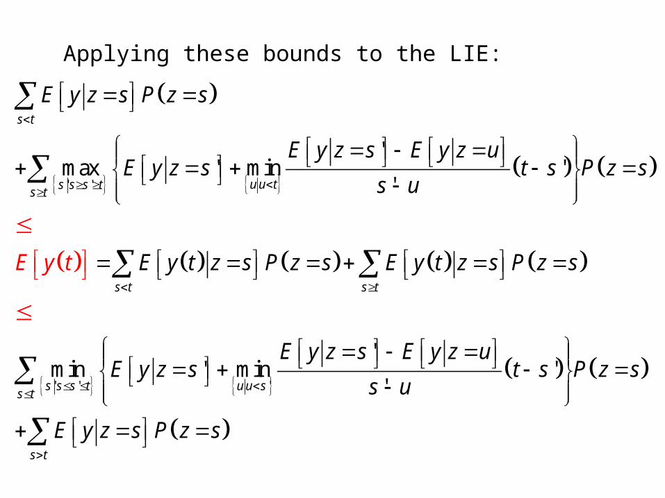
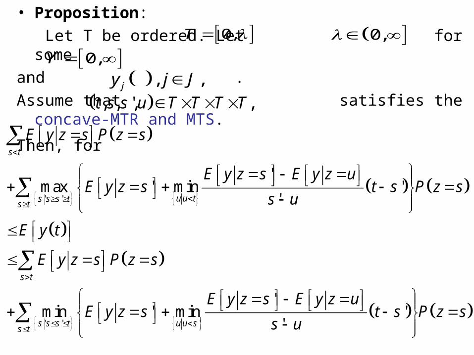
Applying these bounds to the LIE:

' '

' ' '

'max ' min '

'

'min ' min '

'

s t

u u ts s s ts t

s t s t

s s s t u u s

E y z s P z s

E y z s E y z uE y z s t s P z s

s u

E y t z s P z s E y t z s P z s

E y z s E y z u

E

E

y

ts

t

y z s su

s t

s t

P z s

E y z s P z s

Applying these bounds to the LIE:

' '

'

'

'

'min ' min '

'

'max ' min '

'u u ts s s ts

s t

s t

s s s t u s

t

t

u

s

E y z s E y z uE y z s t s P z s

s

E y z s P z s

E y t E y t z s P z s

E y z s E y z u

u

E y

E y z s t ss

t z

u

s P z s

s

s t

t

E y z

P

s P z s

z s

Applying these bounds to the LIE:

'

' '

'

'

'min

'max '

'

min '

min ''

'

s t

s t

s s s t u u s

u u ts s s ts t

s t

E y z s E y z uE y z s t s

E y z s P z s

E y t z s P z s

E y z s E y z uE y

P z ss u

E y t E y t z s P z

z s t su

s

s

s

s t

t

E y z

P z

s P z s

s

Our bounds on

' '

' ' '

'max ' min '

'

'min ' min '

'

s t

u u ts s s ts t

s t s t

s s s t u u s

E y z s P z s

E y z s E y z uE y z s t s P z s

s u

E y t E y t z s P z s E y t z s P z s

E y z s E y z uE y z s t s

s u

s t

s t

P z s

E y z s P z s

E y t

• These bounds are sharp,

since it is possible to take the concave-MTR and MTS functions of

attaining the lower and upper bounds.

, , (or, ) for Tjy j J E y z s

' ' '

The following functions attain the UPPER bounds.

For

,min min ,

where ,

'min ' min

s s s t

s s s t u u s

s t

UB s t E y z sE y z s E y z s s E y z t

t s

UB s t

E y z sE y z s

' .'

For

E y z ut s

s u

s t E y z s E y z s

The following functions attain the LOWER bounds.

For , , , where

'* , * ,, , min min '* , '* , ,

'* , * ,

wher

s s s

s t E y z s LB s

E y z s s t E y z u s tLB s t E y z s s t s s t E y z s

s s t u s t

' '

'e '* , & * , are the solutions of max ' max '

'

For , min , , ,

s s s t u u t

E y z s E y z us s t u s t E y z s t s

s u

s t E y z s E y z s LB t t

'

' ' '

The following functions attain the UPPER bounds.

For

,min min ,

min

'where , min ' min

u u ss s s t

s s s t u u s

s t

UB s t E y z sE y z s s

E y z s t s

E y z t

E y z sUB s t E y z s

' .'

For

E y z ut s

s u

s t E y z s E y z s

B

s’

A

C

t

y

E[y|z = u]

E[y | z = s]

u s

t

E[ y(t) | z = s ]

E y z s

E y z t

s’

C

A

t

y

E[y|z = u]

E[y|z= s]

u s

E[y(t)|z = s ]

E y z s

The following functions attain the LOWER bounds.

For , , , where

'* , * ,, min min '* , min '* , ,

'* , * ,u u ts s s

s t E y z s LB s

E y z s s t E y z u s tLB s E y z s s t s s t E y z s

s s t u s t

' '

'where '* , & * , are the solutions of max ' min '

'

For , min , ,

u u ts s s t

E y z s E y z us s t u s t E y z s t s

s u

s t E y z s E y z s LB s

s’

C

A

t

y

E[y|z = u]

E[y|z= s]

u s

E[y(t)|z = s ]

s

E y z s

E y z s

The following functions attain the LOWER bounds.

For , , , where

'* , * ,, min min '* , '* , ,

'* , * ,

where

s s s

s t E y z s LB s

E y z s s t E y z u s tLB s E y z s s t s s t E y z s

s s t u s t

' '

''* , & * , are the solutions of max ' min '

'

For , min , ,

u u ts s s t

E y z s E y z us s t u s t E y z s t s

s u

s t E y z s E y z s LB t

• The introduction of the assumption of concavity into MTR-MTS assumptions narrows the width of the bounds on

by

' '

' ' '

'max ' max '

'

'min ' min '

'

s s s t u u ts t

s s s t u u ss t

E y z s E y z uE y z s t s E y z t

s u

P z s

E y z s E y z uE y z t E y z s t s

s u

P z

s

E y t

The sharp bound on

the average treatment effect (Returns to schooling)

2

22

1

1 1

1 2 2 1

2' ' '

' '

,

'min ' min '

'

'max ' max

'

s t

s s s t u u ss t

s t

s s s t u u t

t t E y t E y t

E y z s P z s

E y z s E y z uE y z s t s P z s

s u

E y z s P z s

E y z s E y z uE y z s

s u

1

1 's t

t s P z s

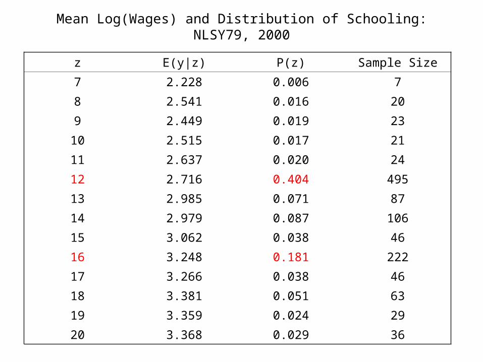
Data

• The 2000 wave of

National Longitudinal Survey of Youth (NLSY)

• White male, year-round full-time workers,

not self-employed, and the ages 35 -- 45.

• Sample size: 1225 individuals

• The same data as Manski&Pepper’s (2000), but most recently available data.

• t : Schooling years, y : log(wage)

z E(y|z) P(z) Sample Size

7 2.228 0.006 7

8 2.541 0.016 20

9 2.449 0.019 23

10 2.515 0.017 21

11 2.637 0.020 24

12 2.716 0.404 495

13 2.985 0.071 87

14 2.979 0.087 106

15 3.062 0.038 46

16 3.248 0.181 222

17 3.266 0.038 46

18 3.381 0.051 63

19 3.359 0.024 29

20 3.368 0.029 36

Mean Log(Wages) and Distribution of Schooling: NLSY79, 2000

Our Bounds on E[y(t)]

2.2

2.4

2.6

2.8

3.0

3.2

3.4

8 9 10 11 12 13 14 15 16 17 18 19 20

Schooling

E[y(

t)]

Our Lower Bound

Our Upper Bound

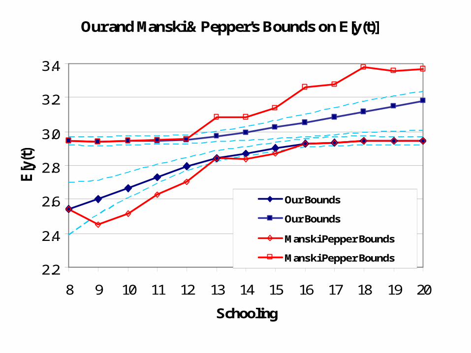
Our and Manski & Pepper's Bounds on E[y(t)]

2.2

2.4

2.6

2.8

3.0

3.2

3.4

8 9 10 11 12 13 14 15 16 17 18 19 20

Schooling

E[y

(t)]

Our Bounds

Our Bounds

Manski Pepper Bounds

Manski Pepper Bounds

Our Bounds, Manski & Pepper's Bounds, Manski Bounds on E[y(t)]

0.0

1.0

2.0

3.0

4.0

5.0

6.0

8 9 10 11 12 13 14 15 16 17 18 19 20

Schooling

E[y

(t)]

Our Bounds

Manski Pepper Bounds

Mansk Bounds

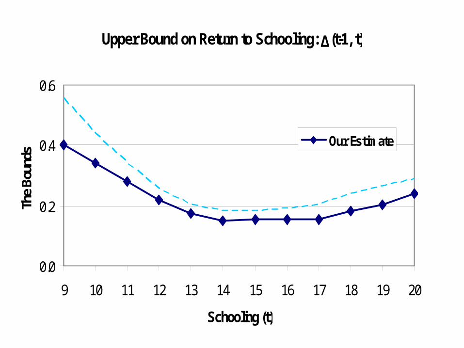
Upper Bound on Return to Schooling: ∆(t-1, t)

0.0

0.2

0.4

0.6

9 10 11 12 13 14 15 16 17 18 19 20

Schooling (t)

The

Bou

nds

Our Estimate

Upper Bound on Return to Schooling: ∆(t-1, t)

0.0

0.2

0.4

0.6

0.8

9 10 11 12 13 14 15 16 17 18 19 20

Schooling (t)

The

Boun

ds

Our Estimate

Manski and Pepper'sEstimate

Upper Bound on Return to Schooling: ∆(t-1, t)

0.0

0.5

1.0

1.5

2.0

2.5

3.0

9 10 11 12 13 14 15 16 17 18 19 20

Schooling (t-1,t)

The

Boun

ds

Our Estimate

Manski and Pepper'sEstimateManski's Estimate

Upper Bounds on

• Card (1999,HLE) surveyed the point estimates on the returns to schooling from the previous studies

using parametric methods.

1,t t

1, 0.052 0.132t t

Ours

(Concave-MTR, MTS)

Manski&Pepper

(MTR, MTS)

Manski

(Concave, MTR)

s t Estimate (0.95 Q) Estimate (0.95 Q) Estimate (0.95 Q)

13 14 0.150 (0.182) 0.240 (0.307) 1.418 (1.515)

12 16 0.257 (0.308) 0.556 (0.612) 2.398 (2.522)

Average effect 0.064 (0.077) 0.139 (0.153) 0.600 (0.630)

Conclusion• Identify the sharp bounds on the mean

treatment response under Concave-MTR and MTS assumptions.

• Empirical application to the returns to schooling• Compare our estimates with those using only

Concave-MTR (Manski (1997)) and using only MTR-MTS (Manski and Pepper (2000)).

• Our bounds are substantially smaller and closer to the point estimates on the existing literature.

Future Research• Develop the testing methods using Blundell,

Gosling, Ichimura and Meghir (2006) and test the concavity or MTS assumptions.