POVERTY DYNAMICS IN RURAL VIETNAM: WINNERS AND LOSERS DURING REFORM

PATRICIA JUSTINO AND JULIE LITCHFIELD

Poverty Research Unit at Sussex and Department of Economics, University of Sussex, UK

ABSTRACT

This paper identifies the transmission mechanisms of the impact of trade reforms on household poverty

dynamics, based on data from a panel of rural Vietnamese households. Poverty dynamics are modelled

using multinomial logistic regressions of poverty transition outcomes. These models are shown to

provide important insights into the behaviour of poor households that cannot be explicitly derived from

household consumption models. We find that changes in household poverty status in Vietnam are

strongly correlated with price and employment changes induced by the trade reforms. These results are

robust to shifts in the poverty line and changes in model specification.

JEL codes: C23; I32; O53.

Keywords: Poverty dynamics, trade liberalisation, economic reform, panel data, Vietnam.

Corresponding author: Patricia Justino, Poverty Research Unit at Sussex, School of Social Sciences and Cultural Studies, University of Sussex, Falmer, Brighton BN1 9SJ, UK. Tel. +44 1273 877402. E-mail: a.p.v.justino@sussex.ac.uk Acknowledgements: We are grateful to Bob Baulch, Rhys Jenkins, Neil McCulloch, Andy McKay, Howard White and, in particular, Alan Winters, for useful discussions and to Yoko Niimi and Puja Vasudeva-Dutta for excellent research assistance. We would also like to thank the participants of seminars and conferences at Sussex (November 2001 and January 2003), Nottingham (April 2002), Hanoi (September 2002) and the 2002 International Association of the Review of Income and Wealth conference (Stockholm) for helpful comments. This paper is part of the project “The Impact of Trade Reforms and Trade Shocks on Household Poverty Dynamics” (ESCOR-R7621) funded by the UK Department for International Development as part of their Globalisation and Poverty Research Programme. Views and opinions expressed in this paper are, however, those of the authors alone. We are grateful to the World Bank for making the trade data available for the DFID-funded Globalisation and Poverty Research Programme’s projects on Vietnam.

1. INTRODUCTION

One of the most visible signs of globalisation is the expansion of international trade generated by

increased trade liberalisation and reductions in trade barriers. This tendency towards greater openness is

believed to provide opportunities for many people, especially those in developing countries. At the same

time, certain individuals may not benefit from the opportunities generated by trade liberalisation, and

may even suffer from trade reforms and the resulting vulnerability to trade shocks. However, very little is

known about the responses of households to economic shocks caused by recent trade reforms.1 In

particular, the dynamics of poverty, i.e. movements into and out of poverty, and the contrast between

persistent and transient poverty have so far been largely overlooked in the development literature in

general and in the trade literature in particular.

This paper is driven by two broad motivations. The first is the explicit empirical analysis of the

transmission mechanisms of trade-induced shocks on household poverty dynamics. We examine how the

macroeconomic changes that took place in Vietnam during the 1990s were transmitted to each individual

household and why some households have benefited more than others from the reforms. This analysis is

based on panel data for 3494 rural households collected in Vietnam in 1992-93 and 1997. This data set

allows us to track the same households during a period of trade reform, and before and after the

occurrence of trade shocks, thereby eliminating unobserved differences between households that are

fixed over time.

The second motivation is largely methodological and refers to the modelling of poverty dynamics. The

direct modelling of poverty outcomes is usually subject to criticisms, notably the fact that its results are

based on arbitrarily defined poverty lines imposed on the total distribution of household consumption or

income, the ‘real’ behavioural variables. Focusing our attention on poverty outcomes, rather than the

whole distribution, may, however, be preferable if the determinants of welfare have different returns to

1 See Dercon (2000), McCulloch, Winters and Cirera (2001) and Winters (2002).

2

the poor and the non-poor.2 Our analysis makes use of multinomial logit regressions adapted to the

analysis of discrete and mutually independent poverty transition outcomes.3 We compare the results of

these models with those of consumption regression models and show that multinomial logit regressions

can successfully be used to model household poverty dynamics without loss of information. Our results

show further that, by focusing on households below the poverty line, rather than the whole distribution,

we obtain valuable insights on the behaviour of poor households that cannot be derived from reduced-

form consumption functions.

The paper is organised as follows. Section 2 describes the household data sets used in the analysis.

Section 3 provides a description of the key trade and other economic reforms and discusses how these

have impacted on the dynamics of household poverty in Vietnam, using both micro-data from the

household surveys and macroeconomic data. We focus on two important trade-related reforms: (i)

liberalisation of agriculture markets for outputs and inputs (including price controls on rice and other

crops and fertilisers) and (ii) liberalisation of export markets, following the removal of export quotas and

tariffs. The bulk of our empirical analysis is carried out in section 4. This section investigates the

relationship between poverty dynamics and trade reforms, controlling also for household- and

community-related characteristics. This relationship is modelled using a multinomial logit regressions

adapted to the analysis of poverty transition outcomes. Those models allow us to estimate the

probabilities of a household (i) staying poor in both years, (ii) escaping poverty, (iii) falling into poverty

or (iv) remaining above the poverty line in both years. Section 5 provides a decomposition of the impact

of trade reforms and other household characteristics on the probability of a household escaping poverty.

The results of sections 4 and 5 show a strong link between poverty dynamics and shocks caused by the

trade reforms. These results are compared to those of continuous consumption growth OLS regression

model and quintile regressions, in section 6. Section 7 concludes the paper.

2 See Appleton (2002) for a detailed discussion of this issue and the application of poverty functions to Uganda survey data. 3 Another example is Glewwe et al. (2002). Our paper takes however this analysis some steps further by explicitly testing the empirical applicability of the multinomial logit models and comparing their results with those of consumption models.

3

2. DATA

The results presented and discussed in this paper are based on micro-data from the Vietnam Living

Standards Measurement Survey (VLSS) for 1992-93 and 1997-98. The VLSS data is obtained from

nation-wide household surveys conducted in 1992-93 (October 1992 to October 1993) and 1997-98

(December 1997 to December 1998), and contains valuable information on 4800 households and 120

communes surveyed in 1992-93 and 6000 households and 150 communes interviewed in 1997-98.4

These surveys are particularly useful as they allow the construction of a panel of 4303 households

interviewed in both years.

Given that only two time periods are available, it is not possible to analyse the duration of poverty spells

or to determine the extent of persistent poverty in Vietnam.5 However, the panel feature of the VLSS data

allows one to track across the five years those households that have remained poor, have moved out of

poverty or have fallen into poverty and determine which particular household characteristics are

associated with those movements.

Although the two VLSS samples are individually representative of the population, the panel is not truly

representative of the whole or rural population (see Haughton, Haughton and Phong, 2001). While this is

a common feature of panel studies in developing countries (see Deaton, 1997 for a discussion), analysis

of the panel does provide an important insight into what happened in rural Vietnam during the 1990s.

The VLSS contains a detailed expenditure questionnaire that allows the construction of standard

indicators of living standards. Most of the analysis in this paper is of household expenditure per capita

per year using a general food and non-food poverty line.6 An individual is defined as being poor if annual

4 These surveys were conducted by the Vietnam’s General Statistical Office and the Ministry of Planning and Investment, with financial assistance from the United Nations Development Programme (UNDP) and the Swedish International Development Agency (SIDA) and technical assistance from the World Bank. 5 See Jenkins (1998) and Devicienti (2000) for analyses of poverty dynamics in the UK when several survey years are available. 6 Unfortunately the VLSS income data, including data on wages, is rather weak, which prevents an analysis of income (as opposed to expenditure) poverty dynamics or of the effect of trade reform on wages.

4

household consumption expenditure per capita is below a poverty line of 1160 thousand dongs per year

per person in 1992-93 and 1790 thousand dongs per year per person in 1997-98.7 The VLSS also

contains a wealth of information on household demographics, ethnicity, education, health, economic

activities, production and employment, assets and a range of community level information on

infrastructure and services.

The analysis developed in this paper is based on the sub-panel of 3494 rural households. Vietnam is

predominantly a rural economy: 78% of all households in Vietnam in 1997-98 lived in rural areas (80%

in 1992-93) and 61% of all Vietnamese households were employed in the agriculture sector in 1997-98

(65% in 1992-93). The decision to analyse rural households only is further supported by the fact that the

two key economic reforms implemented in Vietnam (reform of rice pricing and rice trade and de-

collectivisation of the agricultural sector) were aimed at the rural sector.8

3. TRADE REFORMS AND POVERTY IN VIETNAM

Vietnam is one of the success stories in the attack on poverty in developing countries. The economic and

social changes experienced by Vietnam have been largely ascribed to the “doi moi”, or renovation

policies (World Bank, 1999; CIEM, 2000; Haughton, Haughton and Phong, 2001), designed in 1986 and

implemented during the early 1990s,9 which aimed at transforming Vietnam into an outward-oriented

economy. The “doi moi” policies included the removal of many price controls, the decollectivisation of

land, the provision of greater autonomy to the private sector, the reduction or removal of trade barriers

7 The values are based on the cost of a basket of food items that provide the minimum amount of 2100 calories per person per day plus a non-food component. For a detailed discussion of poverty measurement issues in Vietnam see Litchfield and Justino (2003). 8 Our analysis does not consider movements between the rural and urban sectors. Although rural-to-urban migration is undoubtedly an important phenomenon, the VLSS do not track households that migrate. The VLSS do, however, have data on remittances that will be used in our analysis (see section 4). Dang and Le (2002) report that remittances have become an important source of household income in Vietnam during the later 1990s. 9 Economic reforms, in particular agricultural reforms, started earlier in the late 1970s. However, the ‘Doi Moi’ process that started in 1986 comprised a larger commitment to economic reforms and their extension to the whole economy (see World Bank, 1999).

5

and the opening up of the Vietnamese economy to foreign direct investment.10 The largest and most

visible economic changes took place in Vietnam’s export sector, particularly in the rice market, where

many tariffs were reduced or eliminated. Export rice quotas also increased significantly and the private

sector was allowed a greater role in the production and export of rice. Rice production and rice exports

increased sharply during the 1990s (table 1), turning the country from a net rice importer to the world’s

second largest exporter of rice in 1997 after Thailand (in quantity terms).11 Increases in land titling,

removal of price controls and other trade reforms have also affected the markets for other agriculture

crops (particularly coffee) and industrial products (especially, marine products, textiles and garments,

footwear and food processing) (table 1).12

Despite the commitment of the Vietnamese government to the new economic and trade liberalisation

programmes, the trade regime in Vietnam was quite restrictive until quite late in the 1990s, and involved

a high level of state intervention (see Niimi, Vasudeva-Dutta and Winters, 2002; Nielsen, 2002).

Notwithstanding these restrictions, Vietnam’s gross domestic product per capita grew at an average of

almost 7% per annum during the period between 1993 and 1998, real consumption increased

significantly and overall employment grew at a rate of almost 2% in the same period (table 1).

These economic improvements were accompanied by sharp decreases in poverty across the rural and

urban sectors and across most socio-economic groups (table 2) and to significant movements of

households out of poverty (table 3).13 The decline in poverty rates was, however, more pronounced for

some groups: urban households, households living in the south of the country,14 individuals belonging to

a household with a Kinh head (the majority ethnic group)15 and individuals for whom the households

10 Although flows of foreign direct investment in Vietnam were close to zero during the 1980s, they averaged around 5% of the country’s GDP in the second half of the 1990s (Dollar, 2002). 11 Vietnam’s exports of rice in volume terms made up 17% of total world rice exports in 1997. However, this corresponded to 5% in value terms (which puts Vietnam as the sixth largest exporter of rice in value terms in 1997). The lower value share is due to the inferior quality of Vietnamese rice (Nielsen, 2002). 12 For a more detailed account of trade-related reforms in Vietnam see Niimi, Vasudeva-Dutta and Winters (2002). 13 Litchfield and Justino (2003) describe in more details the trends in poverty in Vietnam during the 1990s as well as testing the sensitivity of the fall to choice of poverty line and to choice of equivalence scale. 14 Vietnam is divided into seven administrative regions (from north to south): Northern Uplands, Red River Delta, North Central, Central Coast, Central Highlands, South East and Mekong River Delta. 15 The VLSS specifies eight ethnic groups, usually categorised for analytical convenience into the majority Kinh, the ethnic Chinese (a special group that includes a small minority of quite well-off households) and the remaining ethnic groups

6

head had a white collar job experienced much sharper falls than other groups (table 2). Furthermore,

examination of the urban and rural panel households reveals that a significant number of Vietnamese

(28.73% overall; 34.19% in the rural sector) remained poor in 1997-98 and a small proportion fell into

poverty (4.74% overall; 5.34% in the rural sector) (table 3).16 Again, the aggregate figures mask

differences for sub-groups of the population.

What is the association between the macroeconomic changes induced by the trade reforms implemented

in Vietnam during the 1990s and these poverty changes? Although economists have long been interested

in the welfare effects of trade liberalisation, much of the empirical analysis has focused on changes in

wages and employment of different categories of workers (for instance, skilled versus unskilled workers

as in Wood, 1994) and relatively little is known about the impact of trade reforms on poverty. Winters

(2002) provides a conceptual framework for analysing the links between trade liberalisation and

household poverty. He identifies a set of transmission mechanisms from trade reform and shocks to

household poverty: direct effects via prices, wages and employment and indirect effects via changes in

public revenues and expenditure. The identification of these changes in the household data will allow us

to determine how each household has responded to the economic reforms.

In the case of Vietnam, household living standards are likely to have been significantly affected by the

large increase in the exports of agricultural crops (particularly, rice and coffee) and industrial products

(especially, marine products, textiles and garments, processed food and footwear) that took place in the

country during the 1990s (table 1). Our analysis focuses on two main mechanisms of transmission: (i)

changes in the prices of agriculture crops and inputs (such as fertilisers), which resulted from the

elimination of trade tariffs and increases in export quotas, and (ii) the creation of new employment

opportunities in the main export industries.

aggregated together. See van de Walle and Gunewardena (2001) and Baulch et al. (2002) for more detailed analyses of the social and economic position of ethnic groups in Vietnam. 16 Litchfield and Justino (2003) found further that consumption inequality increase in Vietnam between 1992-93 and 1997-98.

7

3.1. Agriculture sector changes

The trade reforms implemented in Vietnam triggered changes in the prices of commodities for which

higher export quotas were established and tariffs were removed. Changes in prices, in turn, were likely to

have affected nominal and real incomes of households in their capacity as producers or consumers of

agriculture crops, if price changes were transmitted to the internal markets.17 The effect of price changes

(or shocks if the market is already open) depends on how households respond to these changes or, in

other words, on whether they can accommodate shocks or adapt by, for instance, switching to more

profitable crops (Glewwe and Hall, 1998; McCulloch, Winters and Cirera, 2001; Winters, 2002).

Part of the “doi moi” reforms were aimed at encouraging small farm households to reduce dependence on

rice production and the new agricultural household model advocated diversification across “rice,

orchards and ponds”, i.e. more productive rice production, cultivation of fruit trees and other tree crops

and utilisation of water for rearing ducks for eggs and other forms of aquaculture. Fertiliser supply

constraints were also significantly reduced with the removal of restrictions on imports.18 The success of

the reforms and their impact on average living standards can thus be investigated by examining shifts in

production, changes in productivity and changes in prices. Table 4 illustrates the changes in output and

productivity of the chief agricultural activities and table 5 shows the evolution of prices of key crops over

the period. We discuss first changes in the production of rice and then turn to other agricultural products.

Rice is the main staple for Vietnamese households, comprising 42% of all food expenditure (51% for

households below the poverty line) and 75% of all calorific intake of a typical Vietnamese household

(Minot and Goletti, 1998). National rice security was traditionally provided by a restrictive rice export

quota and most rural households in 1992-93 were engaged in the production of rice: table 2 shows that of

the 3494 rural panel households, 2986 cultivated rice. Since some of the most significant and visible “doi

17 Governments may continue to fix the internal prices of goods which they have officially liberalised internationally (Winters, 2002). See McCulloch, Winters and Cirera (2001) and Winters (2002) for a theoretical analysis of these transmission mechanisms. 18 After 1991, central and provincial state-owned enterprises that earned foreign exchange were allowed to import fertilisers directly (Benjamin and Brandt, 2002)

8

moi” reforms took place in the rice market, where many tariffs on inputs were reduced and export quotas

increased, it is likely that the liberalisation of the rice markets, the rising trend in international rice prices

and the decline in the price of fertilisers (table 5) would have created incentives for households to

increase rice output and productivity. Table 4 shows that the quantity of rice produced in Vietnam

increased by almost 35% between 1992-93 and 1997-98. There was also a significant intensification of

rice productivity as the increase in rice production was accompanied by a small decrease in the number

of households producing rice and a dramatic fall in the area cultivated with rice.19 This is likely to reflect

improvements in technology used in the cultivation of rice, including access to cheaper fertilisers, but

also the diversification of agriculture encouraged by the new agricultural household model.20

Although rice remained a key crop for many farmers, the reforms do seem to have encouraged farm

diversification. Conditions for farm diversification improved as farmers experienced increases in rice

productivity and were able to benefit from relaxation of import tariffs on inputs such as seeds,

machinery, and fertilisers (Thang, 2002). As a consequence, the production and area cultivated of non-

rice crops and other agricultural products increased significantly in Vietnam between 1992-93 and 1997-

98, indicating an intensification of agriculture diversification (table 4).21 The largest production increases

were those of coffee (almost 200%),22 annual industrial crops and fruit crops. Although rice production

grew at over 6% per year, production of annual industrial crops, coffee and fruit crops grew over three

times that rate. Furthermore, whilst the area of land cultivated with rice decreased between 1992-93 and

1997-98, the area cultivated with non-rice crops increased on average by over 200% in the same period.

19 Note that the drastic decrease in the area cultivated with rice between 1992-93 and 1997-98 (93.56%) hides changes in land concentration. While in 1992-93, 96% of all households in the rural panel did not have any rice land, this percentage decreased to 59% in 1997-98. Furthermore, in 1992-93, most (61.4%) rice plots of households that cultivated rice were over 5000m2, which explains the large average of land cultivated with rice in 1992-93, in comparison with the 1997-98 average. In 1997-98, most plots were between 100m2 and 5000m2. If we average the total area cultivated with rice over the whole panel we get a value of 382.39m2 for 1992-93 and 251.60m2 for 1997-98, which represents a lower - but still significant - decrease (34.2%) in the average land cultivated with rice. 20 In fact, rice productivity (measured by kilos of rice harvested per square metre of land cultivated with rice) for those households that produce rice increased by 14.3% between 1992-93 and 1997-98. 21 See Benjamin and Brandt (2002) for similar results. 22 Vietnam started to produce coffee intensively in the Central Highlands after 1995, following a boom in the world price of coffee (Thang et al., 2001). This resulted in a large increase in the exports of coffee from Vietnam, which grew at an annual average of 58.2% between 1993 and 1998 (table 1).

9

Furthermore, prices of most agricultural outputs increased significantly during the period. With the

exception of non-rice food crops and livestock,23 the price of all agriculture crops produced in Vietnam

increased significantly between 1992-93 and 1997-98. Table 5 shows changes in the prices24 of rice and

coffee between 1993 and 1998. The table shows a large increase in the international price of coffee and

in the unit values of coffee. The table also shows that the unit values of rice and paddy obtained from the

VLSS followed a similar trend to international prices, although the unit values of rice have increased by

more than three times the increase in the price of paddy.25 Coffee prices, both internationally and

domestically rose strongly between 1993 and 1998. The price rises for the key staple (rice) and what can

be seen as the key new crop (coffee), combined with increased productivity in rice and other agriculture

products, suggest that net producers at least will have benefited from the “doi moi” liberalisation

programme.

3.2. Employment changes

Although it is likely that the chief impact of the “doi moi” on poverty was via prices, given that the

majority of the rural population is employed in agriculture, it is possible that the stimulation of the rural

economy, increased foreign direct investment and opening of the economy to imports may have affected

poverty via employment and wages. Unfortunately, Vietnamese wage data is very scarce so the effect can

only be measured via employment.26 This effect is likely to be particularly strong in the main export

industries: aquaculture, textiles and garments, processed food and footwear all show a strong increase in

the value of exports over the 1990s (table 1).27 The rural panel data shows further an enormous increase

in the land devoted to aquaculture, as well as significant increases in output values (table 4).

23 This was possibly due to smaller than expected increases in the demand between 1992-93 and 1997-98 for non-rice foods (meat, oils, fish, fruit and vegetables) (Benjamin and Brandt, 2002). 24 The VLSS surveys do no report household-level prices but allow for the calculation of unit values instead. Although these may be subject to measurement error (see Deaton, 1997), commune prices, collected by VLSS researchers, may also suffer from measurement error as the observations did not necessarily involve an actual purchase (VLSS, 2001:21). For completeness we report both sets of prices here. 25 Edmonds and Pavenik, 2002, find a similar divergence between paddy and rice prices. 26 As stated earlier, the VLSS is very weak on income data. The only other source of wage data is the labour survey conducted by the Ministry of Labour, Invalids and Social Affairs from 1995 but unfortunately micro-data was not publicly available. 27 See Niimi, Vasudeva-Dutta and Winters (2002) for more detailed analysis of these changes.

10

However, employment effects seem likely to have been small. Table 6 illustrates the employment in the

main export sectors of members of the rural panel28 and shows that only a very small number of rural

households has any members working in one of the four export industries. Given the large changes in the

exports of seafood, processed food, textiles and footwear, a much bigger employment shift would have

been expected. There are a number of possible explanations, either that much of the predicted increased

employment is of existing family labour, or of previously underemployed paid labourers, or that the

employment effects are found mostly in urban areas and thus not captured in our analysis (see Niimi,

Vasudeva-Dutta and Winters, 2002).

3.3. Movements in and out of poverty

It is possible to examine if the increases in production of rice, coffee and other agriculture crops,

combined with strong rising prices for many products, and productivity gains for some, are reflected in

movements in and out of poverty. Table 6 illustrates these movements for household that produce rice,

coffee and other crops. The table shows that more rice-producing households are poor in both years than

households that do not produce rice. However, fewer rice producing rural households fell into poverty

and more rice producing rural households moved out of poverty in 1997-98. Similar results were

obtained for households that produce non-rice crops, particularly coffee. Furthermore, the percentage of

coffee and other crops producing households that fell into poverty in 1997-98 was significantly lower

than that of households that produce rice, whilst the percentage of coffee producing households that

moved above the poverty line in 1997-98 was significantly higher. This suggests that, although increases

in rice output, prices and productivity have benefited a significant number of Vietnamese households,

increased diversification into other crops between the two survey years has also contributed significantly

towards the reduction of poverty in Vietnam during the same period.

28 The variables that represent the number of household members working in export industries were constructed using the list of profession codes provided in the household surveys. Seafood includes in 1992-93 ‘fishermen, hunters and related workers’ and ‘aquaculture and fishing’ in 1997-98. Food processing includes ‘food, food stuff and beverage processors’ in 1992-93 and ‘food processing’ in 1997-98. Textiles includes ‘spinners, weavers, knitters, dyers and related workers’ and ‘tailors, dressmakers,

11

Employment effects are less obvious (table 8). In general, individuals belonging to rural households that

had at least one member working in one of the main export industries had a higher probability of having

fallen into poverty in 1997-98 than households with no members employed in the export sectors.

However, the probability of escaping poverty is also higher for those rural households. Of these,

households with members working in the seafood industry had the highest probability of having fallen

into poverty in 1997-98, whereas households with members working in the footwear industry registered

the lowest probability of having fallen below the poverty line and the highest probability of having

moved out of poverty in 1997-98.

In summary, the analysis developed in this section shows some tentative links between the economic

reforms implemented in Vietnam after 1986 and changes in poverty status of rural Vietnamese

households. The discussion of trends in output, employment and prices suggest that the strongest effects

will be found via the agricultural production rather than via increased employment. This analysis does

not, however, take into consideration the fact that, over a period of five years, household characteristics

such as demographic composition, education attainment and so forth may have changed and households

may have been subject to shocks (for instance, illness and weather and other covariant risks).29 The next

section provides a formal analysis of the effects of trade reforms on household poverty dynamics, while

controlling simultaneously for demographic and other household-specific characteristics.

sewers, upholsterers and related workers’ in 1992-93 and ‘textile and garment worker’ in 1997-98. Shoemaking includes ‘shoemakers and leather goods makers’ in 1992-93 and ‘leather and shoemaking industry worker’ in 1997-98. 29 In Litchfield and Justino (2003), we found that households in Vietnam have undergone changes that may be associated with

the reduction in poverty observed in the country between 1992-93 and 1997-98: there has been a significant decreased in the

percentage of households headed by a younger individual (and thus more prone to be poor), the number of very large

households decreased by over four percentage points, the number of households with a large number of young children also

decreased significantly (indicating that fewer children were born), the education level of household heads and their spouses

improved sharply and the number of household heads employed in sectors other than the agriculture sector increased. Although

some of these changes may be associated with the economic reforms that took place in Vietnam after 1986, they reflect, to a

large extent, intergenerational changes within the household (panel attrition) as well as the impact of non-economic policies

such as those promoting ‘one-child families’ and literacy-oriented programmes.

12

5. MODELLING POVERTY DYNAMICS IN VIETNAM

The analysis of household poverty dynamics is usually based on models that assess the risk of a

household or an individual remaining poor for a given period of time (Jenkins, 1998; Devicienti, 2000).

However, those models are not suitable for analysis of poverty dynamics between two points in time.

Movements in and out of poverty in Vietnam between 1992-93 and 1997-98 must therefore be modelled

instead using discrete outcome models. We estimate a multinomial logit model of poverty dynamics for

rural Vietnam.

Multinomial logit regressions are commonly used to model processes that involve a single outcome

among several alternatives that cannot be ordered (for example, choices between modes of travelling,

occupational choices, etc).30 Poverty dynamics between two periods can be divided into four mutually

exclusive outcomes: (i) being poor in both periods, (ii) being non-poor in the first period and poor in the

second period, (iii) being poor in the first period and non-poor in the second period and (iv) being non-

poor in both periods.

Multinomial logit models may not, however, be the most adequate method for analysing household

poverty dynamics between two periods if it is believed that there is an implicit ordering of the four

poverty transition outcomes. Although forming a complete ranking of poverty outcomes involves

arbitrary judgements, it may be reasonable to assume that each household will have a set of preferences

regarding the four states.31 Hence, multinomial logit regressions can only be used to determine the

probability of any given household being in one of the above outcomes, if we can show that the four

poverty transition outcomes are independent. We have tested the assumption of independence of

irrelevant alternatives using Hausman tests (Greene, 2000), whose results are reported in the regression

tables. We have also, additionally, estimated a set of conditional logit models, where the rural panel was

30 This is what distinguishes the multinomial logit model from a simple logit model, which analyse factors affecting a binary outcome, and from ordered logit models, which model outcomes that can be ranked. 31 However, Niimi, Vasudeva-Dutta and Winters (2002) estimate a number of ordered logits similar to the specifications here with not very satisfactory results.

13

split into initially poor and non-poor and used a standard binary variable (logit) model used to analyse

the probability of being poor or non-poor in the end year. We did not find significantly different results

between these models and the multinomial logit models. In fact, it can be easily shown that the two types

of model are equivalent (except for sample size and thus standard errors) for outcomes 2 and 3 of the

multinomial logit models, with the advantage that the multinomial logit model estimates simultaneously

the various error terms and thus introduces less measurement error into the analysis.32

The multinomial logit model determines the probability that household i experiences one of the j

outcomes above. This probability is given by:

∑=

== J

k

x

x

iik

ij

e

ejYP

1

'

'

)(β

β

, for j = 0,1,2, ..., J. (1)

where Yi is the outcome experienced by household i, βk are the set of coefficients to be estimated and xi

includes aspects specific to the individual household as well as to the choices. The model is, however,

unidentified since there is more than one solution for β1, ..., βJ that leads to the same probabilities Y = 0,

Y = 1, Y =2, ..., Y = J (Greene, 2000). In order to identify the model, one of the β coefficients must be set

to zero (the base category), and all other sets are estimated in relation to this benchmark. For

convenience we have set β0= 0. In this case, the probability function above becomes:

∑=

+== J

k

x

x

iik

ij

e

ejYP

1

'

'

1)(

β

β

, for j = 1, 2, ..., J. (2)

and

32 Results of this analysis are available from the authors in a more extensive working version of this paper (Justino and Litchfield, 2003). These models are also criticised for the use of arbitrarily defined poverty lines. This issue will be discussed in section 6.

14

∑=

+== J

k

xi

ikeYP

1

'

1

1)0(β

. (3)

In the case of the analysis of poverty dynamics J = 3, where P(Yi=0) is the probability that an individual

belongs to a poor household in both years, P(Yi=1) is the probability of being non-poor in 1992-93 and

poor in 1997-98, i.e. falling into poverty, P(Yi=2) is the probability of being poor in 1992-93 and non-

poor in 1997-98, i.e. escaping poverty, and P(Yi=3) is the probability of a household being non-poor in

both years.

The multinomial logit model described above implies that it is possible to compute J log-odds ratios

[ ] ijiij xPP '0ln β= . The log-odds ratios (also called relative risk ratios) can be normalised on any other

probability, which will yield [ ] )(ln '0 kjjiij xPP ββ −= (Greene, 2000). For convenience

[ ])0()2(ln == ii YPYP and [ )3()1(ln ]== ii YPYP are calculated. These model, respectively, the risks

of a household escaping and falling into poverty.33

This paper presents estimates of three specifications of the multinomial logit model. The first model is

parsimonious in terms of its use of data available in the VLSS but serves as a useful comparison with

other analysis of Vietnamese poverty dynamics, being similar to that of Glewwe, Gragnolati and Zaman

(2002).34 In this model, exits from poverty and entries into poverty are explained by initial characteristics

only:

33 in equation (3) is thus the relative risk ratio for a unit change in the variable x: a relative risk ratio (rrr) of less than one means that the variables increases the probability of the household to be in the base category, whereas an rrr of more than one increases the probability of the household being in the alternative state. The probability is given by the rrr minus one, multiplied by one hundred. For example, in table 9, the value of 1.329 for the Red River Delta means that an household living in the Red River Delta in 1992-93 (in relation to those living in the North Central provinces, the base for the dummy variable) has a 32.9% increase in the probability of having escaped poverty in 1997-98 (in relation to staying poor in both years). Continuous variables have been normalised and their rrr can be interpreted as the effect of a one standard deviation change in the variable on the probability of a household escaping or falling into poverty.

e j ixβ '

34 The two models differ, however, in the choice of explanatory variables and the way they were constructed. Details are provided in Justino and Litchfield (2003).

15

[ ] ),,,,,,,()3()1(ln kiiiiiiiiii CSAEILDFYPYP φ=== (4)

where Fi is a vector of fixed household characteristics (region and ethnicity); Di are household

demographic characteristics (household composition) in 1992-93; Li is the occupation of the head of the

household in 1992-93; Iit is an illness shock dummy for 1992-93;35 Ei is a vector of education levels of

the head of the household and spouse in 1992-93; Ai proxies for household wealth (the net value of

monetary assets,36 land rights, remittances received and access to electricity) in 1992-93; and C is a

vector of commune level institutional and infrastructure characteristics in 1992-93. Finally, in order to

control for noise in the data originating from sampling methods, S

ki

i represents the quarter in which the

household was interviewed. Model 1 can be thought of as the “demographic model”.

Model 2 is the “demographic model with reforms” and incorporates into the above specification Ri, a set

of variables thought to be directly affected by the reforms: production of rice and coffee, a measure of

agriculture diversification (total area cultivated with non-rice crops), whether or not the household has

members employed in at least one of the four main export sectors and the number of household members

working in the main export industries (seafood, food processing, textiles and footwear), plus a set of

variables that account for technological changes possibly induced by the economic reforms. These are

rice productivity (for households that produce rice), the area of land irrigated per capita and the use of

fertilisers.37 The potential impact of land reforms is also incorporated with a dummy variable that takes

the value 1 if the household has extended rights over the land it uses.38

35 This is a dummy variable that takes the value 1 if the head of the household lost more than 7 days of work due to illness in the month prior to the interview and 0 otherwise. 36 Net income assets represent total savings minus debts held by the household. 37 Rice productivity is defined by kilos of rice harvested per square metre of land. In order to avoid measurement errors, this variable has been interacted with a variable indicating whether each household produces rice or not. The rice productivity results refer solely to those households that produce rice. Land irrigation per capita is given by the number of square metres of land irrigation per person in the household. Use of fertilisers was constructed by adding up the amount (kilos) of different fertilisers (urea-nitrogen, phosphate, potassium, NPK and other fertilisers) used by the household in the 12 months prior to the interview. 38 Land was owned solely by the state prior to the ‘Doi Moi’ and land transactions were not permitted. After 1993, land tenure was extended to 20 years for annual crop land and 50 years for perennials. Households were also given extended rights to exchange, transfer, lease, inherit and mortgage land (Benjamin and Brandt, 2002).

16

Models 1 and 2 include only the initial 1992-93 values for the explanatory variables. However, it may be

appropriate to look at changes in explanatory variables as well as the initial characteristics (see Glewwe

and Hall, 1998 and Dercon, 2000). Model 3 thus analyses the relationship between poverty dynamics and

changes in household characteristics, as well as initial conditions as follows:

[ ]),,,

,,,,,,,,,,,,()0()2(ln

iiiki

iiiiiiiiiiiiii

WRRC

SAAEEIILLDDFYPYP

∆

∆∆∆∆∆=== φ (6)

where ∆Di, ∆Ei, ∆Ii and ∆Ai represent changes in the initial demographic, education, illness and wealth

characteristics of each household. Also included are changes in the reform variables, ∆Ri,, namely:

changes in the number of members of the household employed in the four main export industries,39

dummy variables for changes in occupation of the head of the household between the agricultural sector

and other sectors, changes in land irrigated per capita, changes in rice productivity, changes in land

ownership, changes in the quantity of fertilisers used, change in the output of rice and coffee, changes in

the area cultivated with non-rice crops and change in the unit values of rice and coffee. In addition, an

external commune-level shock variable is included to indicate adverse environmental conditions (floods,

droughts, typhoons and other weather-related disasters, or pest damage) between 1993 and 1998 (W ). i

The inclusion of change variables does raise questions of endogeneity, particularly the inclusion of

changes in the variables thought to be affected directly by the economic reforms. This is because these

variables may be simultaneously a cause and a consequence of changes in poverty status. Causality is

therefore less easy to establish but, by including the change variables, we obtain some interesting insights

for valid short-run policy and targeting variables. Endogeneity is partially controlled for by the

simultaneous inclusion of initial values.40

39 Footwear gets dropped from models 2 and 3 because there are not any rural households from the panel working in the footwear industry that are poor. 40 We have in addition analysed how endogeneity may affect the employment variables, as these are the variables most likely to have simultaneously affected and been affected by poverty. We found that 20.91% of all households for which data is available had been in their job in 1997-98 for less than one year, 51.44% between 1-3 years and 27.52% between 3-5 years. This indicates

17

The results for models 1, 2 and 3 are shown in table 9 and are very consistent across the three models,41

with very few statistically significant changes in the relative risk ratios.42 The explanatory power of the

multinomial logit model, measured using a pseudo R2, increases as further variables are added to the base

model. The inclusion of trade variables into the base model explain an extra 20.7% of changes in poverty

status of Vietnamese households between 1992-93 and 1997-8, whereas adding change variables

improve the explanatory power of model 2 by 27.9%.

The regional economic performance in Vietnam during the 1990s suggests the presence of strong

regional effects. Although aggregate growth has been very strong, much of the increase in Vietnam’s

economic performance has taken place in the “growth poles” of Ho Chi Minh City in the Mekong, Hanoi

in the Red River Delta, along the central coast and in the South East, where a large fraction of the

Vietnamese export sector is concentrated. The Mekong River Delta primarily, and Red River Delta to a

lesser extent, are also largely responsible for most of the export quality rice, while coffee production is

concentrated in the Central Highlands. This is reflected in our regression results, which show that

households in southern regions (South East and to a lesser extent households in the Mekong River Delta

and Central Highlands) have increased probabilities of escaping poverty relative to remaining poor in

both years.

In addition to strong regional effects, table 9 shows also significant demographic effects. The results

suggest that the probability of escaping poverty relative to remaining poor is higher than average for

those individuals belonging to households with better educated heads and spouses and older heads.43

Households with heads employed in a white-collar job and households living in communes with better

that the employment variables are unlikely to have been affected by poverty dynamics as almost all households questioned in 1997-98 had been in their jobs for less than 5 years (i.e. since before 1992-93). 41 The standard errors of the estimates for models 1, 2 and 3 are corrected for heteroscedasticity using White’s adjusted heteroscedasticity-consistent variances. 42 The discussion in this section focuses on the relative risk ratios that are statistically significantly different from unity. 43 We believe that this result is associated with the fact that households with young heads are likely to have young children, which poses a financial burden on the household (Litchfield and Justino, 2003). One important cause of higher poverty for households with larger numbers of children is the high costs of education which have soared in Vietnam after the implementation of the new economic reforms (World Bank, 1999).

18

infrastructure have also increased probabilities of having escaped poverty in 1997-98.44 On the other

hand, (non-Chinese) ethnic minorities, as well as households with younger or relatively poorly educated

household heads, not receiving remittances or whose head of household had been absent from work

through illness, were more likely to having fallen into poverty in Vietnam between 1992-93 and 1997-

98.45

Models 2 and 3 show further that household poverty dynamics in Vietnam between 1992-93 and 1997-98

were also significantly affected by variables associated with the reforms that took place in the country

during the 1990s. The models show that individuals belonging to households with members employed in

the seafood industry had increased probabilities of escaping poverty. Furthermore, not only did those

households that in 1992-93 were already involved in the export industries experience higher probabilities

of escaping poverty, but those households which experienced an increase in the number of members

employed in any of the main export industries had increased probabilities of having escaped poverty in

relation to remaining poor in both years. This result suggests that the trade reforms have had important

employment effects for Vietnamese households.

The effects of the trade reforms were also felt strongly in the agriculture sector. The results in table 9

show that individuals belonging to households whose head shifted out of agriculture (as its main

occupation) to any other sector increased the probability of the household escaping poverty by almost

72%.46 Furthermore, although the level of rice output did not seem to affect the probability of households

escaping poverty, larger output levels decreased significantly the probability of households falling into

44 Most institution and infrastructure variables seem to have welfare-enhancing effects. The only exception is access to a post office, which seems to decrease the probability of households escaping poverty and increase the probability of households falling into poverty. This apparently perverse effect may be related to particular characteristics of communes that have post offices: most of these are in the Mekong River Delta, where a relatively large percentage of households fell into poverty. 45 These results are not corrected for household size or economies of scale. Although the conventional wisdom that larger households experience higher probabilities of being poor has been challenged by Lanjouw and Lanjouw (2001) due to findings that the relationship between poverty and household size is not robust to the use of equivalence scales, there is some evidence that in Vietnam the relationship is relatively robust. This may be because economies of scale in rice consumption are small given its staple nature and/or to the relatively small variation in household size among the majority Kinh population. Litchfield and Justino (2003) analyse the results of the multinomial logit models using a poverty line based on per capita consumption with the use of per adult equivalent consumption and find the rrr to be almost identical to the results reported in this paper. 46 This assumes the causality has run from employment to poverty, i.e. that the occupation switch resulted in an improvement in living standards. The alternative is that the household experienced an improvement in living standards for some other reason and subsequently changed occupation. This is an unlikely scenario given the results reported in footnote 40.

19

poverty in 1997-98. At the same time, increases in the retail price of rice increased the probability

households escaping poverty. Coffee production, increases in coffee production and increases in the

retail price of coffee, as well as the cultivation of non-rice crops and increases in the area dedicated to the

cultivation of non-rice crops, have increased and quite large effects on the probability of households

escaping poverty. This result shows that, although improvements in rice productivity and rice prices and

the fall in the cost of fertilisers enabled many rice producers to escape poverty, farmers who were able to

diversify into more profitable crops, such as coffee, experienced greater probabilities of escaping

poverty.

The models analysed in this section allow us thus not only to identify the winners and losers from the

economic reforms but also, based on the examination of the characteristics of each household, to

understand why and how some individuals have benefited more than others from the new economic

policies, at the same time that possible demographic and human capital effects are controlled for.

Welfare-gaining households were, in general, those where a significant number of members found a job

in one of the export sectors and agricultural households more open to diversification of crops and

activities.

6. DECOMPOSING POVERTY DYNAMICS

The regression results obtained above can be used to provide a decomposition of the overall probability

of escaping or entering poverty by each of the explanatory variables, as follows:47

∑∑

∑

= =

== k

i

n

jiji

n

jiji

Y

X

XS

1 1

1

.

β

β (6)

47 See Dercon (2000) for similar analysis.

20

where S is the share of the overall probability of outcome Y, n is the total number of observations in the

panel, k is the total number of coefficients, Xij are the values of the explanatory variables for household i

in period j and iβ are the regression coefficients (not the rrr). Table 10 presents the decomposition of the

probability of a household escaping poverty using the regression coefficients for model 3.48 The table

shows that the largest effects on poverty dynamics in Vietnam between the two survey years were those

of initial level in education of the head of the household and his or her spouse and geographic location.

This latter effect is likely to reflect the impact of economic changes in specific regions, e.g. the increases

in rice productivity in the Mekong River Delta and the establishment of export industries in the South

East, which in turn illustrates the importance of trade reforms for household poverty dynamics.

Initial conditions and reform-induced economic changes contribute also directly (and significantly)

towards changes in household poverty status in Vietnam between 1992-93 and 1997-98. Initial values

and changes in reform-affected agriculture variables account for, respectively 8% and 17.7% of the

probability of escaping from poverty. Employment in the main export industries, and increases in the

number of members employed in those industries, account for further 0.79% and 0.09% of the total

probability of escaping poverty.

The largest contributions to the probability of escaping poverty, among the trade-affected explanatory

factors, are from increases in coffee production and cultivation of non-rice crops. These results confirm

that movements out of poverty in Vietnam between 1992-93 and 1997-98 were, to a relatively large

extent, determined by the trade and trade-related reforms that took place in the country during the 1990s.

7. SENSITIVITY ANALYSIS: POVERTY FUNCTIONS OR CONSUMPTION REGRESSIONS?

Although the multinomial logit models analysed above show consistent and efficient results across three

different model specifications, the choice of regression technique may be subject to criticisms. The

48 The analysis focuses on the probability of escaping poverty as relatively few households became poor during the period.

21

multinomial logit model, like many other discrete poverty outcome models, can be criticised because it

introduces measurement errors by using an arbitrarily defined poverty lines. Reducing a continuous

variable, such as household expenditure, to a qualitative variable may “throw” information away on the

variation in the dependent variable with respect to the variation in explanatory variables (Deaton, 1997).

This is a particularly serious problem in analyses that use developing countries data, since large numbers

of households may be concentrated around the poverty line. There are two ways of tackling this problem.

The first is to test whether the results of the multinomial logit are robust to changes in the poverty

threshold used to define the poverty dynamics outcomes. This analysis is presented in full in Justino and

Litchfield (2003) and shows that considering a poverty line 10% above the official poverty line of 1160

thousand dongs in 1992-93 and 1790 thousand dongs in 1997-98 and another 10% below those values

yields few statistically significantly different results from those presented here in models 1, 2 and 3.

However, discrete poverty outcome models are criticised not just because the choice of poverty line is

arbitrary but also because the outcomes are not derived from a latent continuous variable but from an

observed continuous variable. Therefore, at least in the case of simple probit and logit models, it is

possible to calculate the impacts on the probability of being poor or non-poor from an ordinary

continuous OLS regression. However, the discrete model approach may be preferable to an OLS

approach that imposes constant coefficients across the whole consumption distribution, i.e. for the poor

and the non-poor, if the determinants of welfare have different returns to the poor and the non-poor

(Appleton, 2002). Table 11 shows the (selected) results of an OLS model of the log of real per capita

consumption growth using the same set of explanatory variables as the multinomial logit model 3.49

From these results it is possible to calculate the different elasticities of per capita consumption

expenditure growth relative to household characteristics that remain constant over time (region, tribe and

religion) and household characteristics that changed over time, and hence tentatively determine the

effects of reforms on changes in real household consumption expenditure.50

49 Table 11 presents only selected results – the full set are available from the authors (Justino and Litchfield, 2003). The full set of results includes also a regression using consumption expenditure per adult equivalent as the dependent variable. The estimation of this regression yielded almost identical results to those reported in this paper. 50 This approach is similar to that of Dercon (2000). Our study includes, howver, not only price changes as Dercon’s but also other trade-induced changes. We, provide thus two mechanisms with which to analyse the effects of reforms: (i) changes in

22

The OLS results (model 4) suggest that very few of the trade-related coefficients are statistically

significantly different from zero, and furthermore that the effects of some variables differ from those

obtained in the multinomial logit analysis above. For example, the OLS regressions suggest that living in

the Mekong River Delta has a negative (and statistically significant) impact on consumption growth,

whereas the multinomial logit models suggest the reverse as Mekong River Delta households have a

higher probability of escaping poverty relative to staying poor. It must be remembered that the OLS

model imposes constant parameters across the entire consumption change distribution. The possibility of

obtaining somewhat contradictory results is due to the potential for households to experience decreases in

expenditure but not to become poor, or for households to experience a rise in living standards but not

escape from poverty.

A quintile regression approach can help to examine the behaviour of the consumption growth model

across different expenditure quintiles.51 Table 11 shows the results for the quintile regressions, with the

same set of independent variables as those used in model 3 above. The results of the consumption

quintile regressions show quite clearly that welfare determinants (notably, household size and

composition, education, employment and agriculture production decisions) have different returns to poor

and non-poor households, since the signs of coefficients change from one quintile to another (table 11).

For example, the negative OLS coefficient on the Central Coast dummy is determined by the coefficients

of the second and third quintiles, while the negative OLS coefficient for the MRD dummy is driven by

households in the first quintile. The quintile regressions also show that the impact of larger numbers of

children is particularly damaging (and statistically significantly so) for households in the first three

quintiles despite the positive and statistically significant OLS coefficient. The quintile regressions show

further that the negative coefficients of some of the education variables are driven by the upper quintiles.

trade-related outcomes (employment in export industries and changes in the household production of rice and coffee and cultivation of non-rice crops) and (ii) changes in prices (in this case, changes in the price of rice and coffee). 51 Quintiles are those of per capita household consumption expenditure levels in 1992-93. The independent variable is the difference between the logarithm of consumption expenditure in 1992-93 and 1997-98. The explanatory variables are the ones used in model 3.

23

Higher levels of education have a particularly positive impact on the consumption levels of poor

households (especially those in the second quintile).

The results for the agriculture variables are also illustrative. Despite the negative OLS coefficients, initial

use of fertilisers is associated with consumption growth for those households in the lower quintiles but

not for richer households. Higher initial output levels of rice are associated with declines in consumption

in the OLS model but have divergent and statistically significant impacts on households at opposite ends

of the expenditure distribution. Cultivation of non-rice crops (in particularly, increases in the cultivated

area of non-rice crops) has benefited poorer households, which confirms the earlier findings that

agricultural diversification in Vietnam has had an important and positive impact on the reduction of

poverty in the country between 1992-93 and 1997-98.

These results obtained in the quintile regressions therefore clarify the main differences between the OLS

consumption model and the multinomial logit models. They also provide a bridge between the two

models. However, we believe that the multinomial logit model provides a better method to analyse

poverty dynamics, without introducing significantly large measurement errors into the analysis.

Furthermore, the model has the advantage of focusing our attention directly on how the poor compared to

the non-poor – and not the whole distribution – were affected by the economic and social changes that

took place in Vietnam in the 1990s. Although we can use quintile regressions to infer what type of

household characteristics affect positively or negatively the consumption position of households in

different quintiles, it will not be possible to pinpoint specific households that are welfare-gainers or

welfare-losers following an external shock. This results from the fact that consumption quintile functions

are based on the distribution of households in different consumption quintiles according to their position

in the initial year. This yields limited information about absolute poverty dynamics and has, therefore,

restricted policy relevance. Poverty reduction strategies rely on information on being able to identify the

poor. Because quintile regressions do not allow the analysis of movements within quintiles, policy

makers risk the implementation of inefficient policies that may either include non-poor households or

24

miss altogether poor vulnerable households around the poverty line (drawn within the third quintile in

the case of Vietnam).

8. CONCLUSIONS

This paper demonstrates that it is possible to identify empirically the effects of trade and trade-related

reforms on household poverty dynamics. This is done by modelling poverty dynamics using multinomial

logit regressions that estimate the relative risk of households escaping or falling into poverty - relative to

remaining poor or non-poor, respectively - as a response to trade-induced changes, controlled for other

household characteristics. The analysis focused on two important reforms: (i) liberalisation of agriculture

markets (rice and other crops) and of prices of agriculture crops and inputs (particularly, fertilisers),

which has affected household production decisions, and (ii) liberalisation of export markets, following

the removal of export quotas and tariffs, which has influenced employment patterns of Vietnamese

households.

The results were generally consistent across different model specifications and were shown to be robust

to the use of either discrete or continuous variable models, although the direct analysis of poverty

outcomes proved to be more insightful than the analysis of the whole distribution. We found that the

employment effects were in general positive and had significant welfare-enhancing effects for those

households with members employed in the main export sectors (seafood, food processing, textiles and

garments and footwear). These effects have benefited not only those households that in 1992-93 were

already involved in the export industries, but also those households that increased the number of

members employed in those industries in 1997-98.

The stronger links were, however, those reflected in the position of agricultural households. The results

of our analysis showed that trade reforms that resulted in the increase of prices of agriculture crops and

decrease in fertiliser prices have benefited households that produced rice, coffee and other crops in 1992-

25

93. In particular, increases in agriculture diversification between 1992-93 and 1997-98 significantly

benefited rural households in Vietnam: poverty decreased more notably amongst these households than

amongst households that continued producing mainly rice. This impact was especially strong for the

poorest households.

Despite its generally welfare-enhancing effects, the trade reforms implemented in Vietnam have not

prevented some households from falling into poverty. Furthermore, the world prices of coffee and rice

have decreased significantly since 1998. Although those price changes will not be reflected in our

datasets, it is possible that some coffee- and rice-producing households in Vietnam may have fallen back

into poverty. Although economic changes have yielded large benefits for many Vietnamese households,

a lot still remains to be done in order to ensure that some of the most vulnerable households are able to

cope with the type of socio-economic shocks induced by economic reforms and that clusters of persistent

poverty do not start to form amongst these households. We suggest that policies aimed at promoting

further the diversification of rural incomes by, for instance, encouraging the establishment of small-scale

farm and non-farm enterprises and thereby reducing the dependency of poor rural households on rice

production, would be successful in reducing poverty further.

26

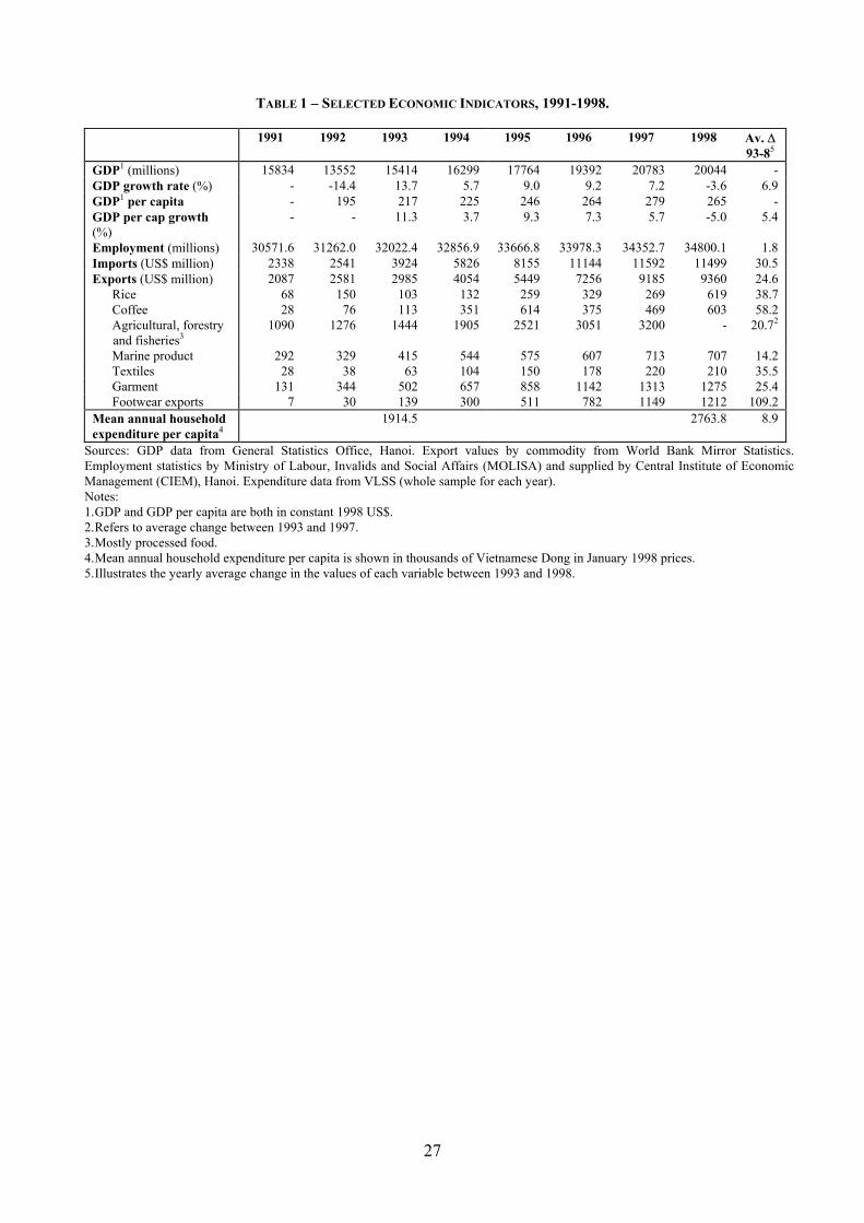
TABLE 1 – SELECTED ECONOMIC INDICATORS, 1991-1998. 1991 1992 1993 1994 1995 1996 1997 1998 Av. ∆

93-85 GDP1 (millions) 15834 13552 15414 16299 17764 19392 20783 20044 - GDP growth rate (%) - -14.4 13.7 5.7 9.0 9.2 7.2 -3.6 6.9 GDP1 per capita - 195 217 225 246 264 279 265 - GDP per cap growth (%)

- - 11.3 3.7 9.3 7.3 5.7 -5.0 5.4

Employment (millions) 30571.6 31262.0 32022.4 32856.9 33666.8 33978.3 34352.7 34800.1 1.8 Imports (US$ million) 2338 2541 3924 5826 8155 11144 11592 11499 30.5 Exports (US$ million) 2087 2581 2985 4054 5449 7256 9185 9360 24.6 Rice 68 150 103 132 259 329 269 619 38.7 Coffee 28 76 113 351 614 375 469 603 58.2 Agricultural, forestry

and fisheries3 1090 1276 1444 1905 2521 3051 3200 - 20.72

Marine product 292 329 415 544 575 607 713 707 14.2 Textiles 28 38 63 104 150 178 220 210 35.5 Garment 131 344 502 657 858 1142 1313 1275 25.4 Footwear exports 7 30 139 300 511 782 1149 1212 109.2 Mean annual household expenditure per capita4

1914.5 2763.8 8.9

Sources: GDP data from General Statistics Office, Hanoi. Export values by commodity from World Bank Mirror Statistics. Employment statistics by Ministry of Labour, Invalids and Social Affairs (MOLISA) and supplied by Central Institute of Economic Management (CIEM), Hanoi. Expenditure data from VLSS (whole sample for each year). Notes: 1. GDP and GDP per capita are both in constant 1998 US$. 2. Refers to average change between 1993 and 1997. 3. Mostly processed food. 4. Mean annual household expenditure per capita is shown in thousands of Vietnamese Dong in January 1998 prices. 5. Illustrates the yearly average change in the values of each variable between 1993 and 1998.

27

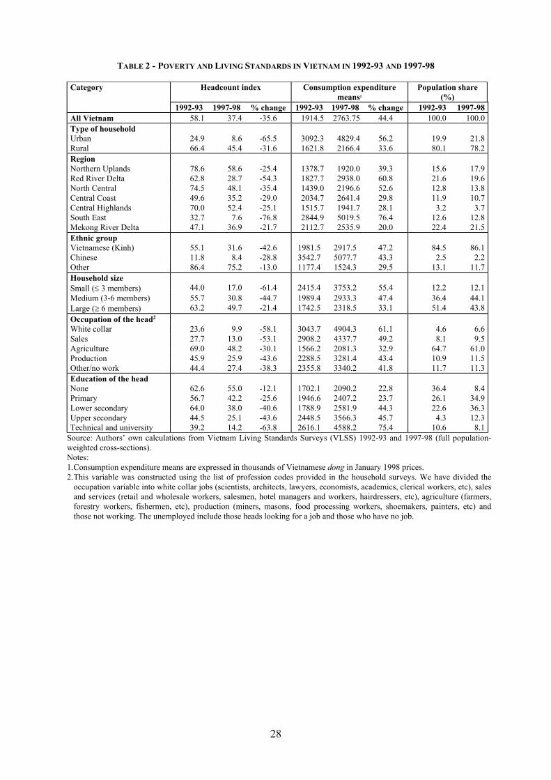
TABLE 2 - POVERTY AND LIVING STANDARDS IN VIETNAM IN 1992-93 AND 1997-98

Headcount index Consumption expenditure means1

Population share (%)

Category

1992-93 1997-98 % change 1992-93 1997-98 % change 1992-93 1997-98All Vietnam 58.1 37.4 -35.6 1914.5 2763.75 44.4 100.0 100.0Type of household Urban 24.9 8.6 -65.5 3092.3 4829.4 56.2 19.9 21.8Rural 66.4 45.4 -31.6 1621.8 2166.4 33.6 80.1 78.2Region Northern Uplands 78.6 58.6 -25.4 1378.7 1920.0 39.3 15.6 17.9Red River Delta 62.8 28.7 -54.3 1827.7 2938.0 60.8 21.6 19.6North Central 74.5 48.1 -35.4 1439.0 2196.6 52.6 12.8 13.8Central Coast 49.6 35.2 -29.0 2034.7 2641.4 29.8 11.9 10.7Central Highlands 70.0 52.4 -25.1 1515.7 1941.7 28.1 3.2 3.7South East 32.7 7.6 -76.8 2844.9 5019.5 76.4 12.6 12.8Mekong River Delta 47.1 36.9 -21.7 2112.7 2535.9 20.0 22.4 21.5Ethnic group Vietnamese (Kinh) 55.1 31.6 -42.6 1981.5 2917.5 47.2 84.5 86.1Chinese 11.8 8.4 -28.8 3542.7 5077.7 43.3 2.5 2.2Other 86.4 75.2 -13.0 1177.4 1524.3 29.5 13.1 11.7Household size Small (≤ 3 members) 44.0 17.0 -61.4 2415.4 3753.2 55.4 12.2 12.1Medium (3-6 members) 55.7 30.8 -44.7 1989.4 2933.3 47.4 36.4 44.1Large (≥ 6 members) 63.2 49.7 -21.4 1742.5 2318.5 33.1 51.4 43.8Occupation of the head2 White collar 23.6 9.9 -58.1 3043.7 4904.3 61.1 4.6 6.6Sales 27.7 13.0 -53.1 2908.2 4337.7 49.2 8.1 9.5Agriculture 69.0 48.2 -30.1 1566.2 2081.3 32.9 64.7 61.0Production 45.9 25.9 -43.6 2288.5 3281.4 43.4 10.9 11.5Other/no work 44.4 27.4 -38.3 2355.8 3340.2 41.8 11.7 11.3Education of the head None 62.6 55.0 -12.1 1702.1 2090.2 22.8 36.4 8.4Primary 56.7 42.2 -25.6 1946.6 2407.2 23.7 26.1 34.9Lower secondary 64.0 38.0 -40.6 1788.9 2581.9 44.3 22.6 36.3Upper secondary 44.5 25.1 -43.6 2448.5 3566.3 45.7 4.3 12.3Technical and university 39.2 14.2 -63.8 2616.1 4588.2 75.4 10.6 8.1

Source: Authors’ own calculations from Vietnam Living Standards Surveys (VLSS) 1992-93 and 1997-98 (full population-weighted cross-sections). Notes: 1. Consumption expenditure means are expressed in thousands of Vietnamese dong in January 1998 prices. 2. This variable was constructed using the list of profession codes provided in the household surveys. We have divided the

occupation variable into white collar jobs (scientists, architects, lawyers, economists, academics, clerical workers, etc), sales and services (retail and wholesale workers, salesmen, hotel managers and workers, hairdressers, etc), agriculture (farmers, forestry workers, fishermen, etc), production (miners, masons, food processing workers, shoemakers, painters, etc) and those not working. The unemployed include those heads looking for a job and those who have no job.

28

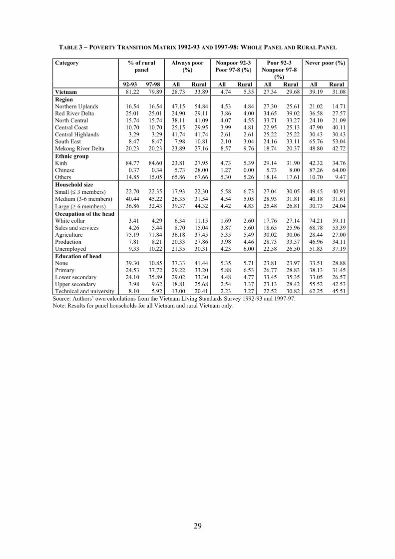
TABLE 3 – POVERTY TRANSITION MATRIX 1992-93 AND 1997-98: WHOLE PANEL AND RURAL PANEL

% of rural panel

Always poor (%)

Nonpoor 92-3 Poor 97-8 (%)

Poor 92-3 Nonpoor 97-8

(%)

Never poor (%)Category

92-93 97-98 All Rural All Rural All Rural All Rural Vietnam 81.22 79.89 28.73 33.89 4.74 5.35 27.34 29.68 39.19 31.08Region Northern Uplands 16.54 16.54 47.15 54.84 4.53 4.84 27.30 25.61 21.02 14.71Red River Delta 25.01 25.01 24.90 29.11 3.86 4.00 34.65 39.02 36.58 27.57North Central 15.74 15.74 38.11 41.09 4.07 4.55 33.71 33.27 24.10 21.09Central Coast 10.70 10.70 25.15 29.95 3.99 4.81 22.95 25.13 47.90 40.11Central Highlands 3.29 3.29 41.74 41.74 2.61 2.61 25.22 25.22 30.43 30.43South East 8.47 8.47 7.98 10.81 2.10 3.04 24.16 33.11 65.76 53.04Mekong River Delta 20.23 20.23 23.89 27.16 8.57 9.76 18.74 20.37 48.80 42.72Ethnic group Kinh 84.77 84.60 23.81 27.95 4.73 5.39 29.14 31.90 42.32 34.76Chinese 0.37 0.34 5.73 28.00 1.27 0.00 5.73 8.00 87.26 64.00Others 14.85 15.05 65.86 67.66 5.30 5.26 18.14 17.61 10.70 9.47Household size Small (≤ 3 members) 22.70 22.35 17.93 22.30 5.58 6.73 27.04 30.05 49.45 40.91Medium (3-6 members) 40.44 45.22 26.35 31.54 4.54 5.05 28.93 31.81 40.18 31.61Large (≥ 6 members) 36.86 32.43 39.37 44.32 4.42 4.83 25.48 26.81 30.73 24.04Occupation of the head White collar 3.41 4.29 6.34 11.15 1.69 2.60 17.76 27.14 74.21 59.11Sales and services 4.26 5.44 8.70 15.04 3.87 5.60 18.65 25.96 68.78 53.39Agriculture 75.19 71.84 36.18 37.45 5.35 5.49 30.02 30.06 28.44 27.00Production 7.81 8.21 20.33 27.86 3.98 4.46 28.73 33.57 46.96 34.11Unemployed 9.33 10.22 21.35 30.31 4.23 6.00 22.58 26.50 51.83 37.19Education of head None 39.30 10.85 37.33 41.44 5.35 5.71 23.81 23.97 33.51 28.88Primary 24.53 37.72 29.22 33.20 5.88 6.53 26.77 28.83 38.13 31.45Lower secondary 24.10 35.89 29.02 33.30 4.48 4.77 33.45 35.35 33.05 26.57Upper secondary 3.98 9.62 18.81 25.68 2.54 3.37 23.13 28.42 55.52 42.53Technical and university 8.10 5.92 13.00 20.41 2.23 3.27 22.52 30.82 62.25 45.51

Source: Authors’ own calculations from the Vietnam Living Standards Survey 1992-93 and 1997-97. Note: Results for panel households for all Vietnam and rural Vietnam only.

29

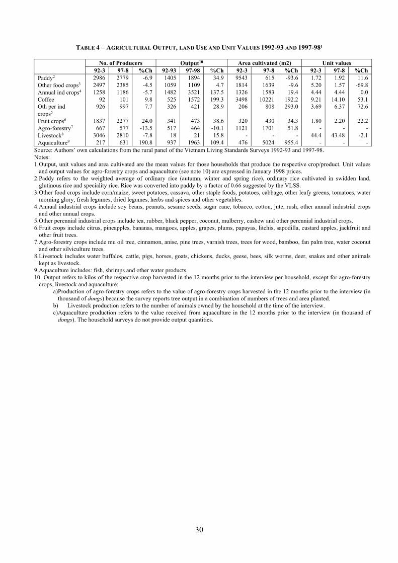
TABLE 4 – AGRICULTURAL OUTPUT, LAND USE AND UNIT VALUES 1992-93 AND 1997-981

No. of Producers Output10 Area cultivated (m2) Unit values 92-3 97-8 %Ch 92-93 97-98 %Ch 92-3 97-8 %Ch 92-3 97-8 %Ch

Paddy2 2986 2779 -6.9 1405 1894 34.9 9543 615 -93.6 1.72 1.92 11.6 Other food crops3 2497 2385 -4.5 1059 1109 4.7 1814 1639 -9.6 5.20 1.57 -69.8 Annual ind crops4 1258 1186 -5.7 1482 3521 137.5 1326 1583 19.4 4.44 4.44 0.0 Coffee 92 101 9.8 525 1572 199.3 3498 10221 192.2 9.21 14.10 53.1 Oth per ind crops5

926 997 7.7 326 421 28.9 206 808 293.0 3.69 6.37 72.6

Fruit crops6 1837 2277 24.0 341 473 38.6 320 430 34.3 1.80 2.20 22.2 Agro-forestry7 667 577 -13.5 517 464 -10.1 1121 1701 51.8 - - - Livestock8 3046 2810 -7.8 18 21 15.8 - - - 44.4 43.48 -2.1 Aquaculture9 217 631 190.8 937 1963 109.4 476 5024 955.4 - - -

Source: Authors’ own calculations from the rural panel of the Vietnam Living Standards Surveys 1992-93 and 1997-98. Notes: 1. Output, unit values and area cultivated are the mean values for those households that produce the respective crop/product. Unit values

and output values for agro-forestry crops and aquaculture (see note 10) are expressed in January 1998 prices. 2. Paddy refers to the weighted average of ordinary rice (autumn, winter and spring rice), ordinary rice cultivated in swidden land,

glutinous rice and speciality rice. Rice was converted into paddy by a factor of 0.66 suggested by the VLSS. 3. Other food crops include corn/maize, sweet potatoes, cassava, other staple foods, potatoes, cabbage, other leafy greens, tomatoes, water

morning glory, fresh legumes, dried legumes, herbs and spices and other vegetables. 4. Annual industrial crops include soy beans, peanuts, sesame seeds, sugar cane, tobacco, cotton, jute, rush, other annual industrial crops

and other annual crops. 5. Other perennial industrial crops include tea, rubber, black pepper, coconut, mulberry, cashew and other perennial industrial crops. 6. Fruit crops include citrus, pineapples, bananas, mangoes, apples, grapes, plums, papayas, litchis, sapodilla, custard apples, jackfruit and

other fruit trees. 7. Agro-forestry crops include mu oil tree, cinnamon, anise, pine trees, varnish trees, trees for wood, bamboo, fan palm tree, water coconut

and other silviculture trees. 8. Livestock includes water buffalos, cattle, pigs, horses, goats, chickens, ducks, geese, bees, silk worms, deer, snakes and other animals

kept as livestock. 9. Aquaculture includes: fish, shrimps and other water products. 10. Output refers to kilos of the respective crop harvested in the 12 months prior to the interview per household, except for agro-forestry

crops, livestock and aquaculture: a) Production of agro-forestry crops refers to the value of agro-forestry crops harvested in the 12 months prior to the interview (in

thousand of dongs) because the survey reports tree output in a combination of numbers of trees and area planted. b) Livestock production refers to the number of animals owned by the household at the time of the interview. c) Aquaculture production refers to the value received from aquaculture in the 12 months prior to the interview (in thousand of

dongs). The household surveys do not provide output quantities.

30

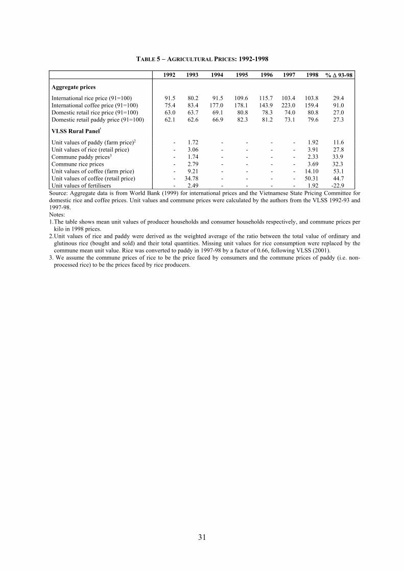
TABLE 5 – AGRICULTURAL PRICES: 1992-1998

1992 1993 1994 1995 1996 1997 1998 % ∆ 93-98

Aggregate prices

International rice price (91=100) 91.5 80.2 91.5 109.6 115.7 103.4 103.8 29.4 International coffee price (91=100) 75.4 83.4 177.0 178.1 143.9 223.0 159.4 91.0 Domestic retail rice price (91=100) 63.0 63.7 69.1 80.8 78.3 74.0 80.8 27.0 Domestic retail paddy price (91=100) 62.1 62.6 66.9 82.3 81.2 73.1 79.6 27.3

VLSS Rural Panel1

Unit values of paddy (farm price)2 - 1.72 - - - - 1.92 11.6 Unit values of rice (retail price) - 3.06 - - - - 3.91 27.8 Commune paddy prices3 - 1.74 - - - - 2.33 33.9 Commune rice prices - 2.79 - - - - 3.69 32.3 Unit values of coffee (farm price) - 9.21 - - - - 14.10 53.1 Unit values of coffee (retail price) - 34.78 - - - - 50.31 44.7 Unit values of fertilisers - 2.49 - - - - 1.92 -22.9

Source: Aggregate data is from World Bank (1999) for international prices and the Vietnamese State Pricing Committee for domestic rice and coffee prices. Unit values and commune prices were calculated by the authors from the VLSS 1992-93 and 1997-98. Notes: 1. The table shows mean unit values of producer households and consumer households respectively, and commune prices per

kilo in 1998 prices. 2. Unit values of rice and paddy were derived as the weighted average of the ratio between the total value of ordinary and

glutinous rice (bought and sold) and their total quantities. Missing unit values for rice consumption were replaced by the commune mean unit value. Rice was converted to paddy in 1997-98 by a factor of 0.66, following VLSS (2001).

3. We assume the commune prices of rice to be the price faced by consumers and the commune prices of paddy (i.e. non-processed rice) to be the prices faced by rice producers.

31

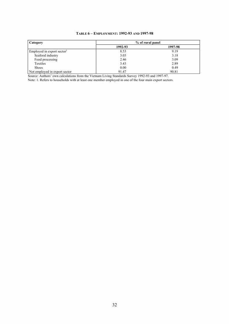
TABLE 6 – EMPLOYMENT: 1992-93 AND 1997-98

% of rural panel Category 1992-93 1997-98

Employed in export sector1 8.53 9.19 Seafood industry 3.03 3.18 Food processing 2.46 3.09 Textiles 3.43 2.89 Shoes 0.00 0.49 Not employed in export sector 91.47 90.81

Source: Authors’ own calculations from the Vietnam Living Standards Survey 1992-93 and 1997-97. Note: 1. Refers to households with at least one member employed in one of the four main export sectors.

32

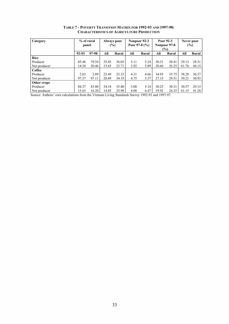
TABLE 7 - POVERTY TRANSITION MATRIX FOR 1992-93 AND 1997-98: CHARACTERISTICS OF AGRICULTURE PRODUCTION

% of rural

panel Always poor

(%) Nonpoor 92-3 Poor 97-8 (%)

Poor 92-3 Nonpoor 97-8

(%)

Never poor (%)

Category

92-93 97-98 All Rural All Rural All Rural All RuralRice Producer 85.46 79.54 35.45 36.05 5.11 5.24 30.31 30.41 29.13 28.31Not producer 14.54 20.46 13.65 23.71 3.92 5.89 20.66 26.25 61.76 44.15Coffee Producer 2.63 2.89 22.49 23.32 4.31 4.66 34.93 35.75 38.28 36.27Not producer 97.37 97.11 28.89 34.19 4.75 5.37 27.15 29.51 39.21 30.93Other crops Producer 84.37 83.80 34.18 35.40 5.00 5.14 30.25 30.31 30.57 29.15Not producer 15.63 16.20 14.85 25.90 4.08 6.47 19.92 26.35 61.15 41.28

Source: Authors’ own calculations from the Vietnam Living Standards Survey 1992-93 and 1997-97.

33

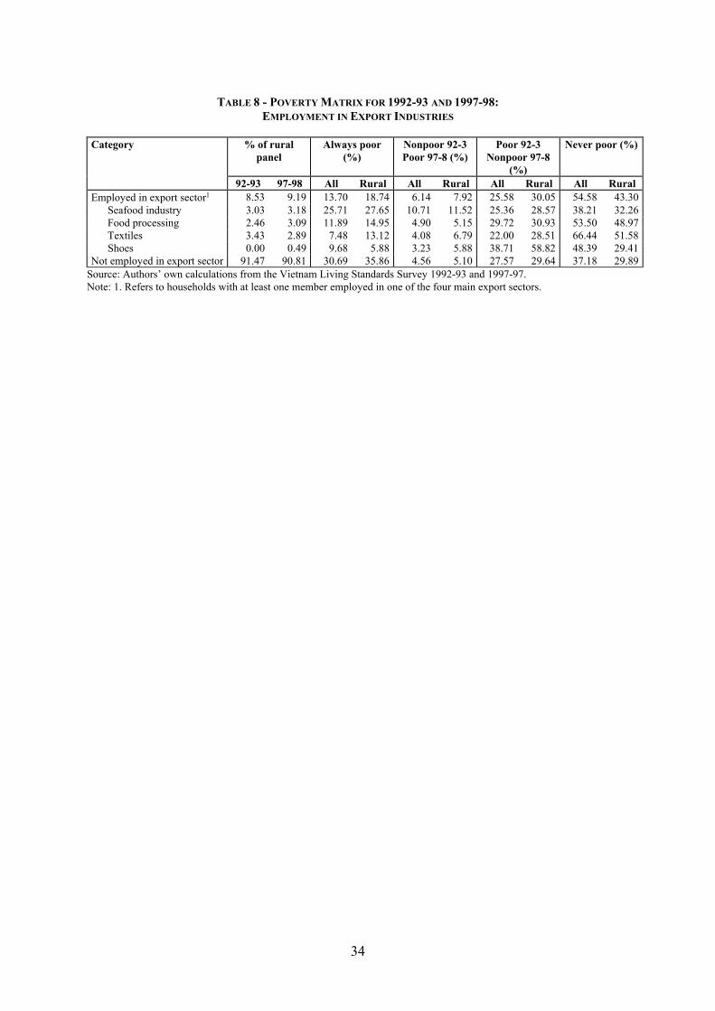
TABLE 8 - POVERTY MATRIX FOR 1992-93 AND 1997-98:

EMPLOYMENT IN EXPORT INDUSTRIES

% of rural panel

Always poor (%)

Nonpoor 92-3 Poor 97-8 (%)

Poor 92-3 Nonpoor 97-8

(%)

Never poor (%)Category

92-93 97-98 All Rural All Rural All Rural All Rural Employed in export sector1 8.53 9.19 13.70 18.74 6.14 7.92 25.58 30.05 54.58 43.30 Seafood industry 3.03 3.18 25.71 27.65 10.71 11.52 25.36 28.57 38.21 32.26 Food processing 2.46 3.09 11.89 14.95 4.90 5.15 29.72 30.93 53.50 48.97 Textiles 3.43 2.89 7.48 13.12 4.08 6.79 22.00 28.51 66.44 51.58 Shoes 0.00 0.49 9.68 5.88 3.23 5.88 38.71 58.82 48.39 29.41Not employed in export sector 91.47 90.81 30.69 35.86 4.56 5.10 27.57 29.64 37.18 29.89

Source: Authors’ own calculations from the Vietnam Living Standards Survey 1992-93 and 1997-97. Note: 1. Refers to households with at least one member employed in one of the four main export sectors.

34

TABLE 9 - POVERTY DYNAMICS IN VIETNAM: MULTINOMIAL LOGIT RESULTS

Model 1 Model 2 Model 3 P→NP NP→P P→NP NP→P P→NP NP→P

Geographic/ethnic characteristics Northern Uplands 1.043 1.193 1.095 1.261 1.114 1.132 Red River Delta 1.329* 0.992 1.118 1.054 0.978 1.104 (North Central) Central Coast 1.298 0.542 1.255 0.586 1.381 0.579 Central Highlands 1.861* 0.219** 0.780 0.330 0.472 0.363 South East 5.544*** 0.291*** 4.589*** 0.264*** 5.229*** 0.270*** Mekong River Delta 2.409*** 0.773 2.151*** 0.943 2.121*** 1.176 (Kinh) Chinese 0.524 0.000*** 0.350 0.000*** 0.404 0.000*** Other ethnicity 0.411*** 2.538*** 0.440*** 2.779*** 0.474*** 2.496*** Buddhist 0.981 0.519*** 1.014 0.516*** 0.945 0.538** (Non-Buddhist) Demographic characteristics Head is male 0.969 0.947 0.915 0.980 1.006 1.030 (Head is female) Head age in 92-93 1.340*** 0.626*** 1.347*** 0.629*** 1.213** 0.666*** Change in head age 1.082 0.895 Head age squared 0.844*** 1.243*** 0.838*** 1.259*** 0.920 1.135 No adults in 92-93 1.077 1.133 0.984 1.235* 0.583*** 1.778*** Change no. adults 0.519*** 2.013*** No children 92-93 0.727*** 0.768** 0.670*** 0.824 0.443*** 1.253 Change no. children 0.343*** 2.962*** Human capital characteristics (Head with no education) Primary school 2.054*** 0.809 2.026*** 0.823 2.047*** 0.832 Lower secondary school 2.992*** 0.518** 2.931*** 0.552** 3.383*** 0.568* Upper secondary school 3.192*** 0.270** 3.046*** 0.265** 3.781*** 0.227** Technical/university 2.260*** 0.297*** 2.287*** 0.309*** 2.636*** 0.358** Change in head education 1.421*** 1.059 Household with no spouse 1.043 0.996 1.100 1.035 1.083 1.007 (Spouse with no education) Primary school 1.116 0.641 1.200 0.628 1.279 0.568* Lower secondary school 1.128 1.003 1.195 1.001 1.324 0.921 Upper secondary school 1.308 1.881 1.391 1.897 1.659 1.546 Technical/university 2.212*** 0.552 2.616*** 0.571 3.270*** 0.515 Change in spouse education 1.157 1.038 Labour market characteristics White collar 3.520*** 0.731 3.745*** 0.676 4.153*** 0.694 Sales 1.283 0.553 1.614 0.390** 1.913* 0.329** (Agriculture) Production 1.038 0.863 1.324 0.689 1.778** 0.492 Not working 0.670** 0.823 0.692* 0.702 0.936 0.522 Change to other occupation in 1997-8 1.719*** 0.794 Change to agriculture in 1997-8 0.781 1.584 Members employed in export sector 1.503 1.583 1.425 1.498 (Not employed in export sector)

35

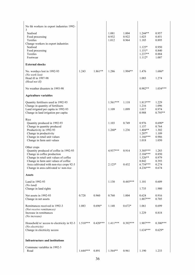
No hh workers in export industries 1992-3

Seafood 1.081 1.004 1.244** 0.957 Food processing 0.932 0.922 1.025 0.851 Textiles 1.012 0.964 1.185 0.895 Change workers in export industries Seafood 1.125* 0.950 Food processing 1.151* 0.840 Textiles 1.237** 0.884 Footwear 1.112* 1.007 External shocks No. wordays lost in 1992-93 1.243 1.861** 1.286 1.994** 1.476 1.686* (No work lost) Head ill in 1997-98 1.083 1.274 (Head not ill) No weather disasters in 1993-98 0.982** 1.034*** Agriculture variables Quantity fertilisers used in 1992-93 1.561*** 1.118 1.813*** 1.229 Change in quantity of fertilisers 1.216 1.096 Land irrigated per capita in 1992-93 1.109 1.099 1.017 0.974 Change in land irrigation per capita 0.988 0.795** Rice Quantity produced in 1992-93 1.103 0.749 0.976 0.690* Change in quantity produced 1.157 0.764 Productivity in 1992-93 1.260* 1.236 1.404** 1.302 Change in productivity 1.207* 1.109 Change in retail unit values 1.166*** 0.986 Change in farm unit values 1.018 1.050 Other crops Quantity produced of coffee in 1992-93 4.937*** 0.914 3.305*** 1.283 Change in coffee production 2.104*** 0.850 Change in retail unit values of coffee 1.326** 0.979 Change in farm unit values of coffee 0.842 0.393 Area cultivated with non-rice crops 92-3 2.125* 0.432 6.754*** 0.274 Change in area cultivated w/ non-rice 4.236*** 0.674 Assets Land in 1992-93 1.130 0.445*** 1.101 0.609 (No land) Change in land rights 1.735 1.980 Net assets in 1992-93 0.728 0.960 0.760 1.004 0.624 0.916 Change in net assets 1.887*** 0.705 Remittances received in 1992-3 1.083 0.696* 1.148 0.672* 1.061 0.699 (Not receive remittances) Increase in remittances 1.229 0.818 (No increase) Household w/ access to electricity in 92-3 1.510*** 0.420*** 1.411*** 0.392*** 1.907*** 0.300*** (No electricity) Change in electricity access 1.634*** 0.629* Infrastructure and institutions Commune variables in 1992-3 Road 1.644*** 0.891 1.564** 0.961 1.190 1.233

36

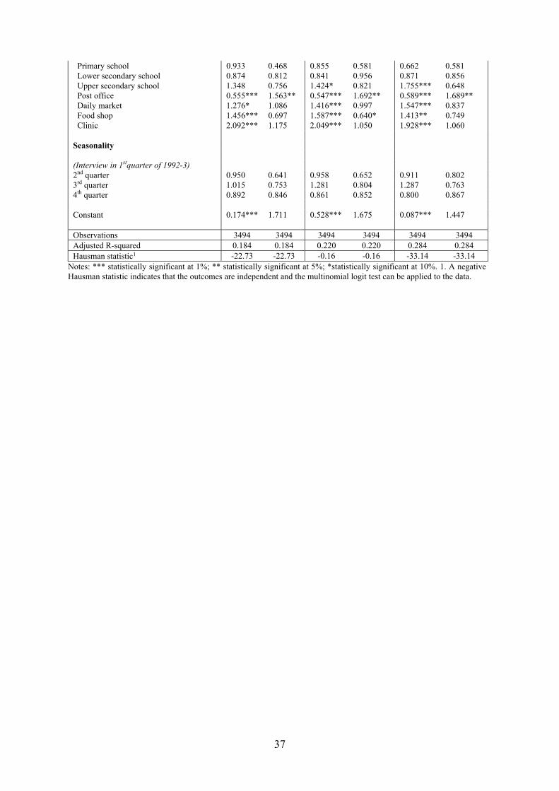
Primary school 0.933 0.468 0.855 0.581 0.662 0.581 Lower secondary school 0.874 0.812 0.841 0.956 0.871 0.856 Upper secondary school 1.348 0.756 1.424* 0.821 1.755*** 0.648 Post office 0.555*** 1.563** 0.547*** 1.692** 0.589*** 1.689** Daily market 1.276* 1.086 1.416*** 0.997 1.547*** 0.837 Food shop 1.456*** 0.697 1.587*** 0.640* 1.413** 0.749 Clinic 2.092*** 1.175 2.049*** 1.050 1.928*** 1.060 Seasonality (Interview in 1stquarter of 1992-3) 2nd quarter 0.950 0.641 0.958 0.652 0.911 0.802 3rd quarter 1.015 0.753 1.281 0.804 1.287 0.763 4th quarter 0.892 0.846 0.861 0.852 0.800 0.867 Constant 0.174*** 1.711 0.528*** 1.675 0.087*** 1.447 Observations 3494 3494 3494 3494 3494 3494 Adjusted R-squared 0.184 0.184 0.220 0.220 0.284 0.284 Hausman statistic1 -22.73 -22.73 -0.16 -0.16 -33.14 -33.14

Notes: *** statistically significant at 1%; ** statistically significant at 5%; *statistically significant at 10%. 1. A negative Hausman statistic indicates that the outcomes are independent and the multinomial logit test can be applied to the data.

37

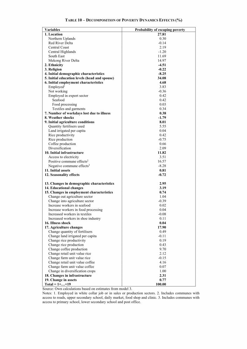
TABLE 10 – DECOMPOSITION OF POVERTY DYNAMICS EFFECTS (%)

Variables Probability of escaping poverty 1. Location 27.81 Northern Uplands 0.30 Red River Delta -0.14 Central Coast 2.19 Central Highlands -1.20 South East 11.69 Mekong River Delta 14.97 2. Ethnicity -4.51 3. Religion -0.22 4. Initial demographic characteristics -8.25 5. Initial education levels (head and spouse) 34.08 6. Initial employment characteristics 4.68 Employed1 3.83 Not working -0.36 Employed in export sector 0.42 Seafood 0.42 Food processing 0.03 Textiles and garments 0.34 7. Number of workdays lost due to illness 0.38 8. Weather shocks -1.79 9. Initial agriculture conditions 8.01 Quantity fertilisers used 5.55 Land irrigated per capita 0.04 Rice productivity 0.42 Rice production -0.75 Coffee production 0.66 Diversification 2.09 10. Initial infrastructure 11.82 Access to electricity 3.51 Positive commune effects2 16.57 Negative commune effects3 -8.28 11. Initial assets 0.81 12. Seasonality effects -0.72 13. Changes in demographic characteristics 2.95 14. Educational changes 3.19 15. Changes in employment characteristics 0.74 Change out agriculture sector 1.04 Change into agriculture sector -0.39 Increase workers in seafood 0.02 Increase workers in food processing 0.04 Increased workers in textiles -0.08 Increased workers in shoe industry 0.11 16. Illness shock 0.04 17. Agriculture changes 17.90 Change quantity of fertilisers 0.49 Change land irrigated per capita -0.11 Change rice productivity 0.19 Change rice production 0.43 Change coffee production 9.70 Change retail unit value rice 2.12 Change farm unit value rice -0.15 Change retail unit value coffee 4.16 Change farm unit value coffee 0.07 Change in diversification crops 1.00 18. Changes in infrastructure 2.31 19. Change in assets 0.77 Total = 1+…+19 100.00

Source: Own calculations based on estimates from model 3. Notes: 1. Employed in white collar job or in sales or production sectors. 2. Includes communes with access to roads, upper secondary school, daily market, food shop and clinic. 3. Includes communes with access to primary school, lower secondary school and post office.

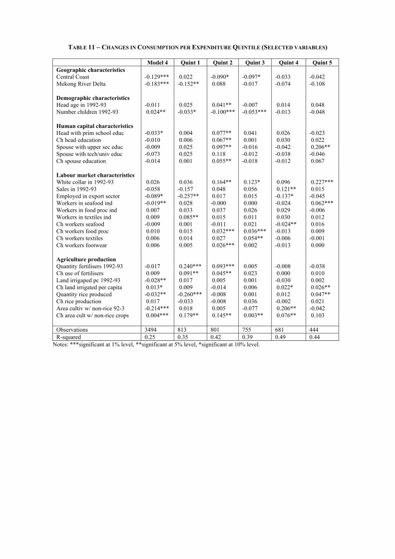
TABLE 11 – CHANGES IN CONSUMPTION PER EXPENDITURE QUINTILE (SELECTED VARIABLES)

Model 4 Quint 1 Quint 2 Quint 3 Quint 4 Quint 5 Geographic characteristics Central Coast -0.129*** 0.022 -0.090* -0.097* -0.033 -0.042 Mekong River Delta -0.183*** -0.152** 0.088 -0.017 -0.074 -0.108 Demographic characteristics Head age in 1992-93 -0.011 0.025 0.041** -0.007 0.014 0.048 Number children 1992-93 0.024** -0.033* -0.100*** -0.053*** -0.013 -0.048 Human capital characteristics Head with prim school educ -0.033* 0.004 0.077** 0.041 0.026 -0.023 Ch head education -0.010 0.006 0.067** 0.001 0.030 0.022 Spouse with upper sec educ -0.009 0.025 0.097** -0.016 -0.042 0.206** Spouse with tech/univ educ -0.073 0.025 0.118 -0.012 -0.038 -0.046 Ch spouse education -0.014 0.001 0.055** -0.018 -0.012 0.067 Labour market characteristics White collar in 1992-93 0.026 0.036 0.164** 0.123* 0.096 0.227*** Sales in 1992-93 -0.058 -0.157 0.048 0.056 0.121** 0.015 Employed in export sector -0.089* -0.257** 0.017 0.015 -0.137* -0.045 Workers in seafood ind -0.019** 0.028 -0.000 0.000 -0.024 0.062*** Workers in food proc ind 0.007 0.033 0.037 0.026 0.029 -0.006 Workers in textiles ind 0.009 0.085** 0.015 0.011 0.030 0.012 Ch workers seafood -0.009 0.001 -0.011 0.021 -0.024** 0.016 Ch workers food proc 0.010 0.015 0.032*** 0.036*** -0.013 0.009 Ch workers textiles 0.006 0.014 0.027 0.054** -0.006 -0.001 Ch workers footwear 0.006 0.005 0.026*** 0.002 -0.013 0.000 Agriculture production Quantity fertilisers 1992-93 -0.017 0.240*** 0.093*** 0.005 -0.008 -0.038 Ch use of fertilisers 0.009 0.091** 0.045** 0.023 0.000 0.010 Land irrigaped pc 1992-93 -0.028** 0.017 0.005 0.001 -0.030 0.002 Ch land irrigated per capita 0.013* 0.009 -0.014 0.006 0.022* 0.026** Quantity rice produced -0.032** -0.260*** -0.008 0.001 0.012 0.047** Ch rice production 0.017 -0.033 -0.008 0.036 -0.002 0.021 Area cultiv w/ non-rice 92-3 -0.214*** 0.018 0.005 -0.077 0.206** -0.042 Ch area cult w/ non-rice crops 0.004*** 0.179** 0.145** 0.003** 0.076** 0.103 Observations 3494 813 801 755 681 444 R-squared 0.25 0.35 0.42 0.39 0.49 0.44

Notes: ***significant at 1% level, **significant at 5% level, *significant at 10% level.

BIBLIOGRAPHY

Appleton, S., 2002. The Rich Are Just Like Us, Only Richer: Poverty Functions or Consumption

Functions?, Journal of African Economies 10 (4), 433-469.

Baulch, R., Chuyen, K., Haughton, D. and Haughton, J., 2000. Ethnic Minority Development in

Vietnam: A Socioeconomic Perspective. Development Research Group, World Bank, Washington

D. C.

Benjamin, D. and Brandt, L., 2002. Agriculture and Income Distribution in Rural Vietnam under

Economic Reforms: A Tale of Two Regions. William Davidson Working Paper no. 519. The

William Davidson Institute, University of Michigan.

CIEM, 2000. Vietnam’s Economy in 1999. Central Institute for Economic Management, Statistical

Publishing House, Hanoi.

Dang Nguyen Anh and Le Kim Sa, 2002. Rural-Urban Labor Migration in Vietnam: New Insights from

the 1999 Population Census. Vietnam’s Socio-Economic Development 30, 69-80.

Deaton, A., 1997. The Analysis of Household Surveys: A Microeconomic Approach to Development

Policy. Johns Hopkins University Press.

Dercon, S., 2000. The Impact of Economic Reforms on Households in Rural Ethiopia 1989-1995. Centre

for the Study of African Economies, Oxford University.

Devicienti, F., 2000. Poverty Persistence in Britain: A Multivariate Analysis Using the BHPS, 1991-

1997. Institute for Social and Economic Research, University of Essex.

Dollar, D., 2002. Reform, Growth and Poverty in Vietnam. Development Research Group, World Bank.

Edmonds, E. and Pavenik, N., 2002. Does Globalisation Increase Child Labour? Evidence from Vietnam.

National Bureau of Economic Research, Working Paper no. 8760.

Glewwe, P. and Hall, G., 1998. Are some groups more vulnerable to macroeconomic shocks than others?

Hypothesis tests based on the panel data from Peru”, Journal of Development Economics 56, 181-

206.

Glewwe, P., Gragnolati, M. and Zaman, H., 2002. Who Gained from Vietnam's Boom in the 1990s?,

Economic Development and Cultural Change 50 (4), 773-792.

40

Greene, W. H., 2000. Econometric Analysis (4th edition). New Jersey: Prentice-Hall.

Haughton, D., Haughton, J. and Phong, N., 2001. Living Standards During and Economic Boom: The

Case of Vietnam. UNDP and General Statistical Office, Hanoi.

Jenkins, S., 1998. Modelling Household Income Dynamics. Institute for Social and Economic Research,

University of Essex.

Justino, P. and Litchfield, J., 2003. Poverty Dynamics in Rural Vietnam: Winners and Losers During

Reform. PRUS Working Paper no. 10. Poverty Research Unit at Sussex, University of Sussex,

Brighton.

Lanjouw, J. O. and Lanjouw, P., 2001. How to Compare Apples and Oranges: Poverty Measurement

based on Different Definitions of Consumption. Review of Income and Wealth, 47 (1), 25-42.

Litchfield, J. and Justino, P., 2003. Poverty Reduction in Vietnam: What Do the Numbers Tell Us?.

Forthcoming in Journal of Asia Pacific Economy.

McCulloch, N., Winters, A. and Cirera, X., 2001. Trade Liberalisation and Poverty: A Handbook.

London: CEPR.

Minot, N and Goletti, F., 2000. Rice Market Liberalisation and Poverty in Viet Nam. Research Report

114, IFPRI.

Nielsen, C. P., 2002. Vietnam in the International Rice Market: A Review and Evaluation of Domestic

and Foreign Rice Policies. Fødevareøkonomisk Institut, Rapport 132.

Niimi, Y., Vasudeva-Dutta, P. and Winters, L. A., 2002. Trade Liberalisation and Poverty Dynamics in

Vietnam. PRUS Working Paper no. 17. Poverty Research Unit at Sussex, University of Sussex,

Brighton.

Thang, N. et al., 2001. Impact of globalisation on poverty. A case study of coffee in Dak Lak province.

Vietnam’s Socio-Economic Development 27, 35-55.

Thang, B. T., 2002. Trade of Fruits and Vegetables in Vietnam. Vietnam’s Socio-Economic

Development 30.

Van de Walle, D. and Gunewardana, D., 2001. Sources of ethnic inequality in Vietnam. Journal of

Development Economics 65, 177-207.

41

42

VLSS, 2001. Vietnam’s Living Standards Survey 1997-98 – Basic Information. Poverty and Human

Resources Division, World Bank.

Winters, L. A., 2002. Trade, Trade Policy and Poverty: What Are the Links? World Economy 25, 1339-

1367.

Wood, A., 1994. North-South Trade, Employment and Inequality: Changing Fortunes in a Skill-Driven

World. Claredon Press, Oxford.

World Bank, 1999. Vietnam Development Report 2000: Attacking Poverty. Joint Report of the

Government, Donor and NGO Working Group, Consultative Group Meeting for Vietnam,

December 14 - 15.