IN DEGREE PROJECT VEHICLE ENGINEERING,SECOND CYCLE, 30 CREDITS

, STOCKHOLM SWEDEN 2016

Path Planning in Unstructured EnvironmentsA Real-time Hybrid A* Implementation for Fast and Deterministic Path Generation for the KTH Research Concept Vehicle

KARL KURZER

KTH ROYAL INSTITUTE OF TECHNOLOGYSCHOOL OF ENGINEERING SCIENCES

Contents

Contents i

List of Figures iii

I Introduction and Theoretical Framework 1

1 Introduction 2

1.1 Relevance of the Topic . . . . . . . . . . . . . . . . . . . . . . . . 2

1.2 Context of the Thesis . . . . . . . . . . . . . . . . . . . . . . . . 3

1.3 Problem Description . . . . . . . . . . . . . . . . . . . . . . . . . 3

1.4 Scope and Aims . . . . . . . . . . . . . . . . . . . . . . . . . . . . 4

1.5 Structure of the Thesis . . . . . . . . . . . . . . . . . . . . . . . . 5

2 Vehicle Platform 6

3 Path Planning 7

3.1 Planning . . . . . . . . . . . . . . . . . . . . . . . . . . . . . . . . 7

3.2 Path . . . . . . . . . . . . . . . . . . . . . . . . . . . . . . . . . . 8

3.3 Basic Problem . . . . . . . . . . . . . . . . . . . . . . . . . . . . 8

3.4 Configuration Space . . . . . . . . . . . . . . . . . . . . . . . . . 8

3.5 Popular Approaches . . . . . . . . . . . . . . . . . . . . . . . . . 9

3.6 Differential/Kinematic Constraints . . . . . . . . . . . . . . . . . 12

4 Collision Detection 15

4.1 Bounding Space and Hierarchies . . . . . . . . . . . . . . . . . . 15

4.2 Spatial Occupancy Enumeration . . . . . . . . . . . . . . . . . . 16

5 Graph Search 18

5.1 Fundamentals . . . . . . . . . . . . . . . . . . . . . . . . . . . . . 18

5.2 Breadth First Search . . . . . . . . . . . . . . . . . . . . . . . . . 21

5.3 Dijkstra’s or Uniform-Cost Search . . . . . . . . . . . . . . . . . 21

5.4 A* Search . . . . . . . . . . . . . . . . . . . . . . . . . . . . . . . 24

5.5 Hybrid A* Search . . . . . . . . . . . . . . . . . . . . . . . . . . . 25

ii CONTENTS

II Method, Implementation and Results 28

6 Method 296.1 Hybrid A* Search . . . . . . . . . . . . . . . . . . . . . . . . . . . 306.2 Heuristics . . . . . . . . . . . . . . . . . . . . . . . . . . . . . . . 336.3 Path Smoothing . . . . . . . . . . . . . . . . . . . . . . . . . . . 33

7 Implementation 387.1 ROS . . . . . . . . . . . . . . . . . . . . . . . . . . . . . . . . . . 387.2 Structure . . . . . . . . . . . . . . . . . . . . . . . . . . . . . . . 38

8 Results and Discussion 408.1 Simulation Results . . . . . . . . . . . . . . . . . . . . . . . . . . 408.2 Real-world Results . . . . . . . . . . . . . . . . . . . . . . . . . . 448.3 Conclusion . . . . . . . . . . . . . . . . . . . . . . . . . . . . . . 44

9 Conclusion 50

10 Future Work 5110.1 Variable Resolution Search . . . . . . . . . . . . . . . . . . . . . 5110.2 Heuristic Lookup Table . . . . . . . . . . . . . . . . . . . . . . . 5110.3 Velocity Profile Generation . . . . . . . . . . . . . . . . . . . . . 5210.4 Path Commitment and Replanning . . . . . . . . . . . . . . . . . 52

Bibliography 53

List of Figures

1.1 Google Trends for the query “autonomous driving” . . . . . . . . 31.2 Depiction of a typical path planning problem to solve . . . . . . 41.3 Obstacle grid . . . . . . . . . . . . . . . . . . . . . . . . . . . . . 4

2.1 Research Concept Vehicle of the ITRL . . . . . . . . . . . . . . . 6

3.1 Configuration space of a robot . . . . . . . . . . . . . . . . . . . 93.2 Rapidly-exploring random tree biased towards unexplored areas . 113.3 Potential Fields . . . . . . . . . . . . . . . . . . . . . . . . . . . . 113.4 Approximate Cell Decomposition . . . . . . . . . . . . . . . . . . 123.5 Kinematic Constraints of a car-like robot . . . . . . . . . . . . . 133.6 Paths of minimal length – Dubins and Reeds-Shepp curves . . . 14

4.1 Collision detection . . . . . . . . . . . . . . . . . . . . . . . . . . 164.2 Bounding regions . . . . . . . . . . . . . . . . . . . . . . . . . . . 174.3 Spatial Occupancy Enumeration . . . . . . . . . . . . . . . . . . 17

5.1 Graph theory explanation . . . . . . . . . . . . . . . . . . . . . . 185.2 Dijkstra’s Algorithm and A* . . . . . . . . . . . . . . . . . . . . 27

6.1 Vertex expansion and pruning . . . . . . . . . . . . . . . . . . . . 326.2 A heuristic comparison . . . . . . . . . . . . . . . . . . . . . . . . 37

7.1 Structure of the program with its inputs and outputs . . . . . . . 39

8.1 The parking structure scenario . . . . . . . . . . . . . . . . . . . 458.2 The obstacle scenario . . . . . . . . . . . . . . . . . . . . . . . . . 468.3 The wall scenario . . . . . . . . . . . . . . . . . . . . . . . . . . . 478.4 The dead end scenario . . . . . . . . . . . . . . . . . . . . . . . . 488.5 Turning on the spot for change of directions . . . . . . . . . . . . 498.6 Parallel parking the car . . . . . . . . . . . . . . . . . . . . . . . 49

List of Algorithms

1 Rapidly-exploring Random Tree . . . . . . . . . . . . . . . . . . . 102 Breadth First Search . . . . . . . . . . . . . . . . . . . . . . . . . 223 Dijkstra’s Search . . . . . . . . . . . . . . . . . . . . . . . . . . . 234 A* Search . . . . . . . . . . . . . . . . . . . . . . . . . . . . . . . 245 Hybrid A* Search . . . . . . . . . . . . . . . . . . . . . . . . . . . 266 Same Cell Expansion . . . . . . . . . . . . . . . . . . . . . . . . . 317 Gradient Descent . . . . . . . . . . . . . . . . . . . . . . . . . . . 36

Abstract

On the way to fully autonomously driving vehicles a multitude of challengeshave to be overcome. One common problem is the navigation of the vehiclefrom a start pose to a goal pose in an environment that does not provide anyspecific structure (no preferred ways of movement). Typical examples of suchenvironments are parking lots or construction sites; in these scenarios the vehicleneeds to navigate safely around obstacles ideally using the optimal (with regardto a specified parameter) path between the start and the goal pose.

The work conducted throughout this master’s thesis focuses on the develop-ment of a suitable path planning algorithm for the Research Concept Vehicle(RCV) of the Integrated Transport Research Lab (ITRL) at KTH Royal Insti-tute of Technology, in Stockholm, Sweden.

The development of the path planner requires more than just the pure al-gorithm, as the code needs to be tested and respective results evaluated. Inaddition, the resulting algorithm needs to be wrapped in a way that it canbe deployed easily and interfaced with different other systems on the researchvehicle. Thus the thesis also tries to gives insights into ways of achieving real-time capabilities necessary for experimental testing as well as on how to setupa visualization environment for simulation and debugging.

Acknowledgments

As this this was written at the ITRL (Integrated Transport Research Lab) I hadthe opportunity to work together with a variety of people from different fields.My sincerest thanks go to my supervisors Mikael Nybacka, John Folkesson andJonas Martensson for their confidence in me and the chance to work on thisinteresting and seminal topic.

Furthermore I want to thank Andreas Hogger for his suggestion of usingC++ in combination with ROS and his continuous support with both, withoutROS the integration into the RCV architecture would have been much morecumbersome. I also want to thank the invaluable asset – Rui Oliveira for alwaysgiving me the opportunity to discuss concepts, ideas and foster understanding.

Additional thanks go to Niclas Evestedt an Erik Ward, who have clarifiedkey questions throughout this thesis and have helped with the integration of thecode on the vehicle.

Special thanks go to Moritz Werling (BMW) who not only initially pointedme in the direction of the topic, but also gave valuable insights with regard tothe algorithm in general. I also want to thank Marcello Cirillo (Scania), whonot only mentioned important implementation details of search algorithms, butasked critical questions that improved the overall quality.

Last but not least I want to thank all people that I had the pleasure workingwith at ITRL and KTH in general. It has been a very pleasurable experiencefor me with a steep learning curve.

Part I

Introduction andTheoretical Framework

Chapter 1

Introduction

On the way to fully autonomously driving vehicles a multitude of challenges haveto be overcome. A crucial part for autonomously driving vehicles is a planningsystem that typically encompasses different abstraction layers, such as mission,behavioral, and motion planning. While the mission planner provides a suitableroute in a road network to arrive at the goal, the behavioral planner determinesappropriate actions in traffic, such as changing lanes as well as stopping atintersections; the motion planner on the other hand operates on a lower level,avoiding obstacles, while progressing towards local goals [38].

An even more specialized problem is the navigation of the vehicle from astart pose to a goal pose in an environment that does not provide any specificstructure; unstructured driving as opposed to structured driving (road follow-ing). Typical examples of such environments are parking lots or constructionsite. In these scenarios the vehicle needs to navigate safely around obstacleswithout any kind of path reference, such as lane markings, ideally using theoptimal1path between the start and the goal pose.

1.1 Relevance of the Topic

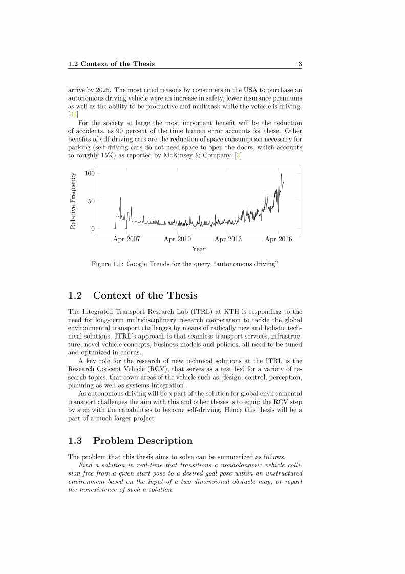
Autonomous driving vehicles might be one of the most publicly discussed andresearched engineering topics at the moment of this writing. While the tradi-tional car makers seem to pick up speed only very slowly, new entrants suchas Alphabet (formerly Google) Comma.ai, drive.ai, Uber in the USA as wellas OXBOTICA in the UK, and ZMP, Robot Taxi and nuTonomy in Asia areaccelerating the advancement in self driving car technology at a rapid pace, re-leasing autonomous vehicles before the decade’s end. A simple query with thesearch term autonomous driving on Google Trends will underline this, revealinga huge increase in search volume over the past six years depicted in Figure 1.1on the facing page.

In a study titled ”Revolution in the Driver’s Seat: The Road to AutonomousVehicles” the Boston Consulting Group defines Tesla’s Autopilot released inOctober 2015 the first stage of several from partial to fully autonomous driving.Furthermore their estimates are, that fully autonomous driving vehicles will

1with regard to a specified parameter, such as time, length, velocity, lateral acceleration,distance to obstacles, etc.

1.2 Context of the Thesis 3

arrive by 2025. The most cited reasons by consumers in the USA to purchase anautonomous driving vehicle were an increase in safety, lower insurance premiumsas well as the ability to be productive and multitask while the vehicle is driving.[31]

For the society at large the most important benefit will be the reductionof accidents, as 90 percent of the time human error accounts for these. Otherbenefits of self-driving cars are the reduction of space consumption necessary forparking (self-driving cars do not need space to open the doors, which accountsto roughly 15%) as reported by McKinsey & Company. [3]

Apr 2007 Apr 2010 Apr 2013 Apr 2016

0

50

100

Year

Rel

ati

veF

requ

ency

Figure 1.1: Google Trends for the query “autonomous driving”

1.2 Context of the Thesis

The Integrated Transport Research Lab (ITRL) at KTH is responding to theneed for long-term multidisciplinary research cooperation to tackle the globalenvironmental transport challenges by means of radically new and holistic tech-nical solutions. ITRL’s approach is that seamless transport services, infrastruc-ture, novel vehicle concepts, business models and policies, all need to be tunedand optimized in chorus.

A key role for the research of new technical solutions at the ITRL is theResearch Concept Vehicle (RCV), that serves as a test bed for a variety of re-search topics, that cover areas of the vehicle such as, design, control, perception,planning as well as systems integration.

As autonomous driving will be a part of the solution for global environmentaltransport challenges the aim with this and other theses is to equip the RCV stepby step with the capabilities to become self-driving. Hence this thesis will be apart of a much larger project.

1.3 Problem Description

The problem that this thesis aims to solve can be summarized as follows.Find a solution in real-time that transitions a nonholonomic vehicle colli-

sion free from a given start pose to a desired goal pose within an unstructuredenvironment based on the input of a two dimensional obstacle map, or reportthe nonexistence of such a solution.

4 INTRODUCTION

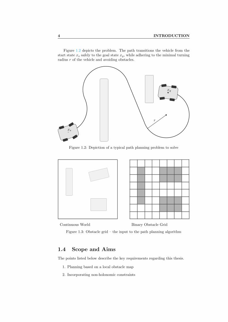
Figure 1.2 depicts the problem. The path transitions the vehicle from thestart state xs safely to the goal state xg, while adhering to the minimal turningradius r of the vehicle and avoiding obstacles.

r

xg

xs

Figure 1.2: Depiction of a typical path planning problem to solve

Continuous World Binary Obstacle Grid

Figure 1.3: Obstacle grid – the input to the path planning algorithm

1.4 Scope and Aims

The points listed below describe the key requirements regarding this thesis.

1. Planning based on a local obstacle map

2. Incorporating non-holonomic constraints

1.5 Structure of the Thesis 5

3. Ensuring real-time capability

4. Performing analysis and evaluation of results

5. Integrating and driving autonomously (optional)

The input to the path planning algorithm is a grid based binary obstaclemap. The second point addresses the fact that the planner should be used forvehicles that cannot turn on the spot, e.g. cars, hence the produced paths mustbe continuous and need to be based on a model of the vehicle. In order to usethe algorithm in a car, it needs to re-plan continuously and perform collisionchecking. For this purpose the actual implementation needs to be as efficient aspossible, thus C++ is a necessity in order to provide the re-planning frequenciesrequired. The development shall include a critical analysis and evaluation ofthe algorithm as well as its results. It is the aim to deploy the software on theRCV and demonstrate its capabilities in a real-world scenario, if time and otherconstraints will allow for it.

The scope of the thesis is to prototypically develop as well as implement apath planning algorithm, hence this focuses on a specific solution rather than ageneral and will not provide a comparison between different approaches as otherworks might do.

1.5 Structure of the Thesis

This thesis is split into two distinct parts. The first part of this thesis willpresent the theoretical foundation, in order to prepare the reader for the ac-tual implementation of the algorithm. Chapter 2 shortly introduces the vehicleplatform the path planning is being developed for. Chapter 3 deals with a briefintroduction into path planning, where the term is dissected and popular ap-proaches are touched on. Chapter 4 focuses on collision detection, as it is a vitalpart for most path planning approaches. And Chapter 5, the last chapter of thefirst part dissects popular graph search algorithms, that form the basis of thiswork.

The second part focuses on the method and its implementation in detail.Chapter 7 uses the theoretical framework to explain the implemented hybridA* search in detail. Chapter 8 is primarily a collection of the results as well asanalysis of the same. Chapter 9 Summarizes the entirety of the thesis, whilestressing the achievements of this particular implementation. And finally chap-ter 10 will give the reader some suggestions regarding future work that can orshould be conducted.

Chapter 2

Vehicle Platform

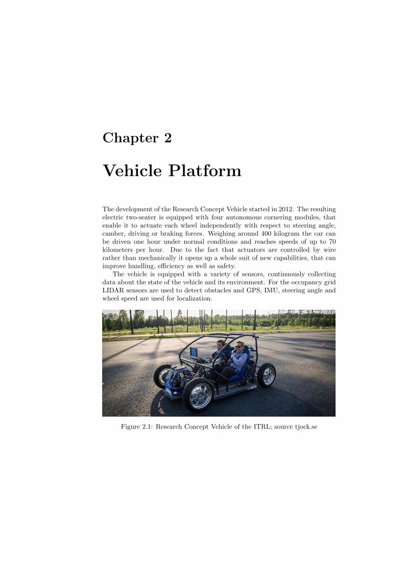
The development of the Research Concept Vehicle started in 2012. The resultingelectric two-seater is equipped with four autonomous cornering modules, thatenable it to actuate each wheel independently with respect to steering angle,camber, driving or braking forces. Weighing around 400 kilogram the car canbe driven one hour under normal conditions and reaches speeds of up to 70kilometers per hour. Due to the fact that actuators are controlled by wirerather than mechanically it opens up a whole suit of new capabilities, that canimprove handling, efficiency as well as safety.

The vehicle is equipped with a variety of sensors, continuously collectingdata about the state of the vehicle and its environment. For the occupancy gridLIDAR sensors are used to detect obstacles and GPS, IMU, steering angle andwheel speed are used for localization.

Figure 2.1: Research Concept Vehicle of the ITRL; source tjock.se

Chapter 3

Path Planning

Fully autonomous robots need to be able to understand high-level commands, asit cannot be the goal to tell the robot how to do a certain thing, but rather whatto do [23]. While autonomous robots need to be able to reason, perceive andcontrol themselves adequately, planning plays a key role. Planning consumesthe robot’s knowledge about the world to provide its actuators (controllers) withappropriate actions (references) to perform the task at hand. Machine learningmay still be one of the largest areas in artificial intelligence, but planning canbe seen as a necessary complement to it, as in the future decisions need to beformed autonomously based on the learned [26].

This section will present and discuss a variety of different planning tech-niques, many of which will not only be applicable to path planning, but arepowerful tools for more general problems [26].

3.1 Planning

First, one should understand the meaning of the word planning. Meriam Web-ster gives the following simple definition:“the act or process of making a planto achieve or do something”. Given this general description it becomes obvi-ous that one can mean very different things by saying the word planning, thefollowing can all be seen as acts of planning.

1. A person who intends to use public transportation to visit someone.

2. A politician who signs a bill to persuade voters.

3. A navigation system that calculates a route for a trip.

Planning in this thesis is understood as the search for a set of actions uthat transitions a given start state to a desired goal state. When planning isconducted by computers one has to do it programmatically, the result is thus aplanning algorithm that usually returns the set of actions that transitions thestart to the goal state. Planning under uncertainty is not considered, such thatstatement number 2 is not considered in this thesis.

8 PATH PLANNING

3.2 Path

If planning returns the set of actions that are necessary to transition from astart to a goal state, then one can say that a path consist of the entire set ofactions, u ∈ Upath as well as the resulting states along the path x ∈ X. Morespecifically a path in this thesis is either the set of actions Upath that move avehicle from a current start state to a desired goal state through the Euclideantwo dimensional plane or the resulting poses p ∈ P, with X → P.

While Latombe uses the term motion planning, Lavalle uses path planning.Their might be some slight differences in the way they can be interpreted, butin general they have been used for the same things.

3.3 Basic Problem

The problem addressed in this thesis shall be further specified and a generalformulation be established. The robot is the only moving object in the world.The dynamics of the robot are not considered, hence removing any time depen-dencies. As collisions shall not occur they will not be modeled either.

Based on these simplifications the basic problem can be described as follows[23,26]:

• A ⊂ W, the robot, is a single moving rigid object in world W representedin the Euclidean space as R2

• O ⊂ W, the obstacles, are stationary rigid objects in W

• geometry, position and orientation of A and O are known a priori

• Problem: given a start and goal pose of A ⊂ W, plan a path P ⊂ Wdenoting the set of poses so that A(p) ∩ O = ∅ for any pose p ∈ P alongthe path from start to goal, terminate and report P or ∅, if a path hasbeen found or no such path exists

3.4 Configuration Space

In the literature of motion planning the concept of the configuration space hasbeen well established, as it facilitates the formulation of path planning prob-lems, presenting various concepts with an underlying scheme yielding greaterexpressive power [23, 26]. Configuration spaces have been extensively used byLozano-Perez in the 80s for the description of spatial planning problems, e.g.the search for an appropriate space to place an object or the search for a pathof an object in an unstructured environment with obstacles [23]. The searchfor the appropriated placement or the path an object should take, is a prob-lem often encountered in design and manufacturing, where compactness needsto be achieved but maintainability shall not be sacrificed. An example of thisis changing a headlight bulb of a car. Manufacturers are trying to build it ascompact as possible, but clearly there is a need for maintainability, as a lightbulb might need to be replaced from time to time. The advantage of the con-figuration space representation is that it reduces the problem from a rigid bodyto a point and thus eases the search [29].

3.5 Popular Approaches 9

Given the robot or agent A ⊂ W, where W is the world as the two di-mensional Euclidean space R2 with a fixed Cartesian coordinate frame FW ,each possible configuration of A(q) can be described by a q of the form (x, y, θ)denoting a position along the x- and y-axis as well as an orientation in FWrespectively. All possible configurations q form the configuration space C ⊂ W.Attached to the robot A is the frame FA, so that FW(q) = FA, this allows thedescription of parts of the robot relative to A and not W. The configurationspace of the robot can be further divided in subsets Cobs and Cfree. The configu-ration space Cobs ⊂ C describes the set of all q where A(q)∪O 6= ∅ and hence therobot is in collision. On contrast Cfree ⊂ C is the set of all safe configurationsq, A(q) ∪ O = ∅. [23, 26]

Since the configuration space only considers the static case, the regions de-fined are not fully descriptive, once dynamics are introduced. In order to in-corporate dynamics, analog to C the state space X can be introduced, withX = C. In addition to C, X allows the description of the dynamics of the robotso that with f : x → q a given state x with (x, y, θ, x, y) can be mapped to qas (x, y, θ). Describing this will add another subset Xric → CXric ⊂ Cfree to X,the region of inevitable collision. This region describes all states that will leadto a collision due to robot’s dynamics. [23, 26]

Figure 3.1 illustrates the configuration space for a robot A. The whitearea,Cfree is safe for any configuration A(q). The light gray areas describepossible collisions with the dark gray areas O and one or more configurationsof A(q).

Cobs

Cfree

Cobs

A(q)

O

Figure 3.1: Configuration space of a robot

3.5 Popular Approaches

As with most problems, there are a variety of different methods for path plan-ning based on the requirements of the problem to be solved. The aim of thissection is not to compare methods for path planning. Each has advantages anddisadvantages, as discussed in many other places, but it should rather give thereader a quick overview over different type of solutions for the same problem.

10 PATH PLANNING

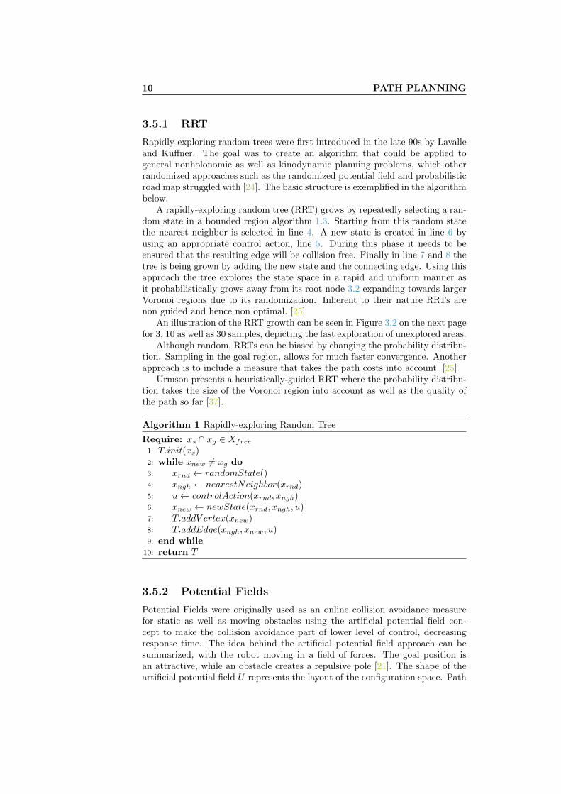
3.5.1 RRT

Rapidly-exploring random trees were first introduced in the late 90s by Lavalleand Kuffner. The goal was to create an algorithm that could be applied togeneral nonholonomic as well as kinodynamic planning problems, which otherrandomized approaches such as the randomized potential field and probabilisticroad map struggled with [24]. The basic structure is exemplified in the algorithmbelow.

A rapidly-exploring random tree (RRT) grows by repeatedly selecting a ran-dom state in a bounded region algorithm 1.3. Starting from this random statethe nearest neighbor is selected in line 4. A new state is created in line 6 byusing an appropriate control action, line 5. During this phase it needs to beensured that the resulting edge will be collision free. Finally in line 7 and 8 thetree is being grown by adding the new state and the connecting edge. Using thisapproach the tree explores the state space in a rapid and uniform manner asit probabilistically grows away from its root node 3.2 expanding towards largerVoronoi regions due to its randomization. Inherent to their nature RRTs arenon guided and hence non optimal. [25]

An illustration of the RRT growth can be seen in Figure 3.2 on the next pagefor 3, 10 as well as 30 samples, depicting the fast exploration of unexplored areas.

Although random, RRTs can be biased by changing the probability distribu-tion. Sampling in the goal region, allows for much faster convergence. Anotherapproach is to include a measure that takes the path costs into account. [25]

Urmson presents a heuristically-guided RRT where the probability distribu-tion takes the size of the Voronoi region into account as well as the quality ofthe path so far [37].

Algorithm 1 Rapidly-exploring Random Tree

Require: xs ∩ xg ∈ Xfree

1: T.init(xs)2: while xnew 6= xg do3: xrnd ← randomState()4: xngh ← nearestNeighbor(xrnd)5: u← controlAction(xrnd, xngh)6: xnew ← newState(xrnd, xngh, u)7: T.addV ertex(xnew)8: T.addEdge(xngh, xnew, u)9: end while

10: return T

3.5.2 Potential Fields

Potential Fields were originally used as an online collision avoidance measurefor static as well as moving obstacles using the artificial potential field con-cept to make the collision avoidance part of lower level of control, decreasingresponse time. The idea behind the artificial potential field approach can besummarized, with the robot moving in a field of forces. The goal position isan attractive, while an obstacle creates a repulsive pole [21]. The shape of theartificial potential field U represents the layout of the configuration space. Path

3.5 Popular Approaches 11

3 Samples 10 Samples 30 Samples

xs

xg

xs

xg

xs

xg

Figure 3.2: Rapidly-exploring random tree biased towards unexplored areas

planning is conducted in a sequential manner. In each step the artificial force~F (q) = −~OU(q) acting on the robot’s current configuration will create a pathincrement towards this direction. [23]

Figure 3.3 shows the resulting potential based on a attractive goal potential(darker areas) and a repulsive obstacle potential (lighter areas). A ball placedanywhere in the resulting potential would naturally (assuming a downward forceacting on the ball, such as gravity) end up in the goal location (lower right) whileavoiding collisions with obstacles.

As obstacle avoidance was the original goal, potential fields come with therisk of not being able to reach the goal as the robot might get stuck in localminima. To work around this inherent characteristic one can try to formulatethe potential function without local minima or incorporate techniques that allowthe escape from the same, such as RRT [26]. [23]

Attractive Potential Repulsive Potential Resulting Potential

Figure 3.3: Potential Fields

3.5.3 Approximate Cell Decomposition

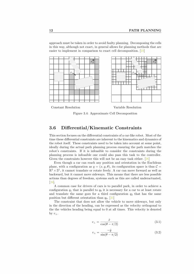
Path planning with approximate cell decomposition can be traced back toBrooks and Lozano-Perez in the mid 80s. The basic idea is to divide the config-uration space into rectangles with edges parallel to the axes of the space. Theresulting cells will be either free, occupied or mixed, depending on the config-uration space of the obstacles intersecting with the respective rectangle or not,see Figure 3.4 on the next page. The search for a path is conducted by findinga set of connected and free cells that include the start as well as the goal con-figuration. [6] Applicable graph search algorithms are explained in more detailin chapter 5 on page 18.

This approach does not represent the free space exactly, hence a conservative

12 PATH PLANNING

approach must be taken in order to avoid faulty planning. Decomposing the cellsin this way, although not exact, in general allows for planning methods that areeasier to implement in comparison to exact cell decomposition. [23]

Constant Resolution Variable Resolution

xs

xg

xs

xg

Figure 3.4: Approximate Cell Decomposition

3.6 Differential/Kinematic Constraints

This section focuses on the differential constraints of a car-like robot. Most of thetime these differential constraints are inherent to the kinematics and dynamics ofthe robot itself. These constraints need to be taken into account at some point,ideally during the actual path planning process ensuring the path matches therobot’s constraints. If it is infeasible to consider the constraints during theplanning process is infeasible one could also pass this task to the controller.Given the constraints however this will not be an easy task either. [26]

Even though a car can reach any position and orientation in the Euclideanplane, with a configuration as q = (x, y, θ), its configuration space is thus C =R2 × S1, it cannot translate or rotate freely. A car can move forward as well asbackward, but it cannot move sideways. This means that there are less possibleactions than degrees of freedom, systems such as this are called underactuated,[26].

A common case for drivers of cars is to parallel park, in order to achieve aconfiguration q1 that is parallel to q0 it is necessary for a car to at least rotateand translate the same goes for a third configuration q2 that has the sameposition but different orientation than q0. [23]

The constraint that does not allow the vehicle to move sideways, but onlyin the direction of the heading, can be expressed as the velocity orthogonal tothe the vehicles heading being equal to 0 at all times. This velocity is denotedby v⊥.

v⊥ =x

cos(θ − π/2)(3.1)

v⊥ =−y

sin(θ − π/2)(3.2)

3.6 Differential/Kinematic Constraints 13

x

cos(θ − π/2)=

−ysin(θ − π/2)

(3.3)

x sin(θ − π/2) + y cos(θ − π/2) = 0 (3.4)

The following describes the non-holonomic constraint.

x cos(θ)− y sin(θ) = 0 (3.5)

Y

X

ϕ θv

v⊥ = 0

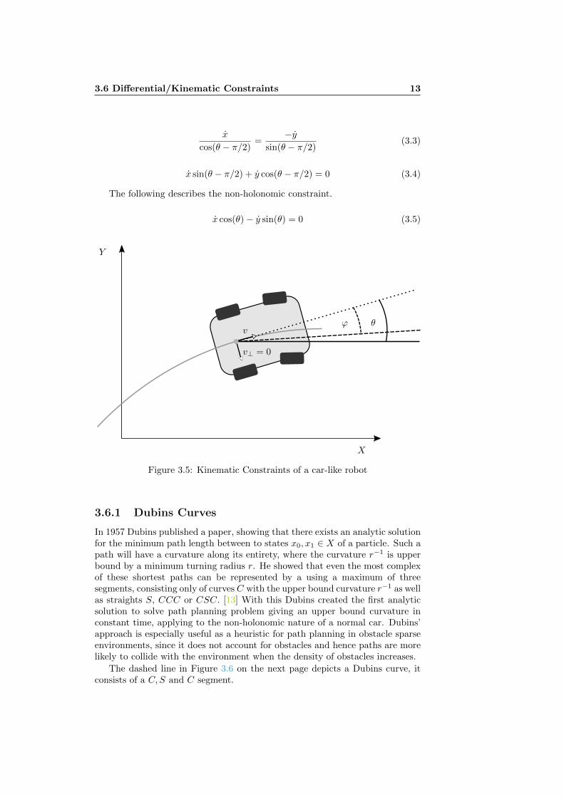
Figure 3.5: Kinematic Constraints of a car-like robot

3.6.1 Dubins Curves

In 1957 Dubins published a paper, showing that there exists an analytic solutionfor the minimum path length between to states x0, x1 ∈ X of a particle. Such apath will have a curvature along its entirety, where the curvature r−1 is upperbound by a minimum turning radius r. He showed that even the most complexof these shortest paths can be represented by a using a maximum of threesegments, consisting only of curves C with the upper bound curvature r−1 as wellas straights S, CCC or CSC. [13] With this Dubins created the first analyticsolution to solve path planning problem giving an upper bound curvature inconstant time, applying to the non-holonomic nature of a normal car. Dubins’approach is especially useful as a heuristic for path planning in obstacle sparseenvironments, since it does not account for obstacles and hence paths are morelikely to collide with the environment when the density of obstacles increases.

The dashed line in Figure 3.6 on the next page depicts a Dubins curve, itconsists of a C, S and C segment.

14 PATH PLANNING

3.6.2 Reeds-Shepp Curves

More than thirty years later in 1990, Reeds and Shepp solved a problem seem-ingly similar to the one of Dubins. They developed a solution for calculatingpaths of upper bound curvature under the assumption that the car could driveforwards as well as backwards. The solution with a maximum of 2 cusps (dueto reversing) can be found among a set of possible paths that will never exceed68. The minimum lenght path in the pool of possible paths is the solution. Justlike Dubins Curves Reeds-Shepp curves also are made up of curved and straightsegments. Due to the possibility of reversing the paths will consist at most offive segments, CCSCC [34]

The solid line in Figure 3.6 depicts a Reeds-Shepp curve, it as well as theDubins curve in this case consists of a C, S and C segment.

r

r

Figure 3.6: Dubins (dashed) and Reeds-Shepp (solid) curves

Chapter 4

Collision Detection

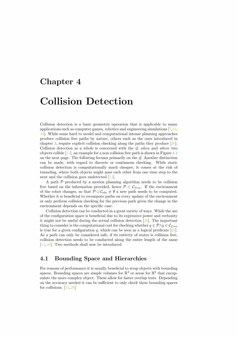
Collision detection is a basic geometric operation that is applicable to manyapplications such as computer games, robotics and engineering simulations [7,14,33]. While some hard to model and computational intense planning approachesproduce collision free paths by nature, others such as the ones introduced inchapter 3, require explicit collision checking along the paths they produce [26].Collision detection as a whole is concerned with the if, when and where twoobjects collide [14], an example for a non collision free path is shown in Figure 4.1on the next page. The following focuses primarily on the if. Another distinctioncan be made, with regard to discrete or continuous checking. While staticcollision detection is computationally much cheaper, it comes at the risk oftunneling, where both objects might pass each other from one time step to thenext and the collision goes undetected [14].

A path P produced by a motion planning algorithm needs to be collisionfree based on the information provided, hence P ⊂ Cfree. If the environmentof the robot changes, so that P ∪ Cobs 6= ∅ a new path needs to be computed.Whether it is beneficial to recompute paths on every update of the environmentor only perform collision checking for the previous path given the change in theenvironment depends on the specific case.

Collision detection can be conducted in a great variety of ways. While the useof the configuration space is beneficial due to its expressive power and verbosityit might not be useful during the actual collision detection [26]. The importantthing to consider is the computational cost for checking whether q ∈ P∧q ∈ Cfreeis true for a given configuration q, which can be seen as a logical predicate [26].As a path can only be considered safe, if its entirety of states is collision free,collision detection needs to be conducted along the entire length of the same[14,26]. Two methods shall now be introduced.

4.1 Bounding Space and Hierarchies

For reasons of performance it is usually beneficial to wrap objects with boundingspaces. Bounding spaces are simple volumes for R3 or areas for R2 that encap-sulate the more complex object. These allow for faster overlap tests. Dependingon the accuracy needed it can be sufficient to only check these bounding spacesfor collisions. [14, 26]

16 COLLISION DETECTION

xs

Collision

Figure 4.1: Collision detection

If higher accuracy is required, hierarchical methods can be implemented,these break up a larger complicated convex bodies into a tree. The tree repre-sents bounding spaces that contain smaller and smaller subsets of the originalobject as depicted in Figure 4.2 on the facing page. This hierachy allows formore accurate geometric description of the object, while reducing the computa-tional cost of intersection testing, since children only need to be tested if theirlarger parents collide. [14, 26]

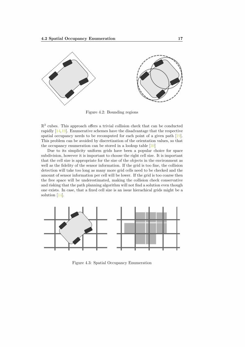
Lavalle and Ericson define some criteria for the choice of appropriate bound-ing spaces.

• The space should fit the object as tightly as possible.

• The intersection test for two spaces should be as efficient as possible.

• The space should be easy to rotate.

Figure 4.2 on the next page illustrates two different ways bounding regionscan be used. On the left a rectangular shape for approximation is used, whileon the right the shape is broken down into a hierarchy with two levels usingcircles for approximation. For the latter a simple intersection test with obstaclesusing circular bounding regions consists of computing the relative distance of thecenters and compute whether or not the distance is greater than die combinedradii of both regions.

4.2 Spatial Occupancy Enumeration

Spatial occupancy enumeration overlays the space with a grid. This subdivisionof space allows the occupancy enumeration of objects, storing an exhaustivearray of grid cells covered by the respective object [14, 19]. The method isdepicted in Figure 4.3 on the facing page. In R2 these might be squares, in

4.2 Spatial Occupancy Enumeration 17

Figure 4.2: Bounding regions

R3 cubes. This approach offers a trivial collision check that can be conductedrapidly [14,19]. Enumerative schemes have the disadvantage that the respectivespatial occupancy needs to be recomputed for each point of a given path [19].This problem can be avoided by discretization of the orientation values, so thatthe occupancy enumeration can be stored in a lookup table [39]

Due to its simplicity uniform grids have been a popular choice for spacesubdivision, however it is important to choose the right cell size. It is importantthat the cell size is appropriate for the size of the objects in the environment aswell as the fidelity of the sensor information. If the grid is too fine, the collisiondetection will take too long as many more grid cells need to be checked and theamount of sensor information per cell will be lower. If the grid is too coarse thenthe free space will be underestimated, making the collision check conservativeand risking that the path planning algorithm will not find a solution even thoughone exists. In case, that a fixed cell size is an issue hierachical grids might be asolution [14].

Figure 4.3: Spatial Occupancy Enumeration

Chapter 5

Graph Search

This chapter explains the basic theory necessary to understand graphs and theterminology associated with it. The later part of the chapter focuses on elabo-rating different graph search algorithms that are fundamental to understandingthe implementation of the search algorithm in this thesis.

5.1 Fundamentals

A graph such as the one depicted in figure 5.1 consists of vertices V as well asedges E. With G being a graph V = V (G), is the set of vertices of the graphand E = E(G), the set of Edges. Edges connect vertices of a graph. An edgeof a graph can be described by x, y, as it connects the vertices x and y. Edgesthat have at least one vertex in common are considered adjacent. Vertices thathave at least one edge in common are called neighboring [4]

Graphs can be either directed or undirected. A directed graph has unidirec-tional edges, a undirected graph has bidirectional edges. In the following theword nodes and vertices might be used interchangeably.

12

3 2 1 4

V2

V4 V5 V6

V3

V7

V1

Figure 5.1: Graph theory explanation

5.1 Fundamentals 19

5.1.1 State Space of a Graph

While the chapter is termed graph search one has to understand that this termcan be seen as the search for a set of actions that changes the state of an objectfrom an initial state to a desired goal state. Given this general descriptiongraph search algorithms can be applied to a great variety of problems frommotion planning to artificial intelligence [26].

The following definition constitutes a general description of the state space ofa graph, it is borrowed from Lavalle’s famous book titled Planning Algorithms.

1. A nonempty state space x ∈ X, which is finite or countably infinite set ofstates.

2. For each state x ∈ X, a finite action space U(x).

3. A state transition function f that produces a state f(x, u) ∈ X for everyx ∈ X and u ∈ U(x). The state transition equation is derived from f asx′ = f(x, u).

4. An initial state xs ∈ X.

5. A goal set XG ⊂ X.

The vertices V of the graph G can be considered the state space X of the G.Thus, each vertex holds information pertaining to a specific state. The edges Eare best represented by the action space U . Where an edge u ∈ U(x) transitionsa state x ∈ X to a state x′ ∈ X with the state transition function f(x, u).

5.1.2 Open and Closed Lists

For the explanation of the following algorithms two types of lists need specialattention. On the one side there is the open list O, representing the set ofthe search frontier, the vertices, that have not yet been expanded, but have anadjacent vertex that has been expanded, hence any vertex vi ∈ O is part of thefrontier. On the other side there is the closed list C, representing the set ofvertices that have already been expanded.

Priority Queues

Depending on the algorithm these lists need to implemented as a priority queue.A priority queue is a data structure that sorts a set by a key either from large tosmall or vice versa. The following operations are supported by the basic priorityqueue. All these actions maintain the order of the queue [36].

• insertion of a given item with a given key

• find the minimum of the keys of the items in the queue

• delete the item with the minimum key from the queue

The type of queue chosen has a considerable impact on the time complexityfor the operations mentioned above. When implementing a queue it is recom-mended to take this into consideration, as a more complex queue might yield

20 GRAPH SEARCH

considerable better performance, especially when operating on larger sets ofdata.1

5.1.3 Heuristics

In order to find an optimal path the search needs to be systematic. Varioussearch algorithms differ most significantly in the way they expand vertices [26].To avoid wasteful search of unpromising regions of a graph the search must be asinformed as possible, only expanding nodes that have the potential to belong tothe optimal path [18]. If the search uses information that leads to skipping theexpansion of a specific node, hence failing to find the optimal path, admissibilityis forfeited. An ideal heuristic returns the real cost of a vertex.

Heuristics are used as an aid for approximating a solution in order to addressthe limitations of processing power, in some cases drastically reducing the searchspace. A finite amount of time only allows for a finite number of calculations.Although this comes without a suprise it still is a major limitation to problemsthat grow exponentially with search depth. While searching a graph the searchneeds to decide which vertex to expand and which edge to take. Informationthat aims to answer this question is considered a heuristic. A heuristic might bebased on some cost estimates between the current vertex and the goal vertex. [32]

A heuristic is a function that provides the necessary information that allowsthe algorithm to converge faster towards the goal. Only an admissible heuristiccan lead to optimal results [18].

5.1.4 Optimality

One of the great advantages of graph search algorithms compared to otherapproaches for path planning is that many algorithms are proven to be optimal.Bellman’s principle of optimality reads below.

An optimal policy has the property that whatever the initial stateand initial decision are, the remaining decisions must constitute anoptimal policy with regard to the state resulting from the first deci-sion. [2]

In essence any optimal solution for a problem that requires a sequence ofdecisions can only consist of optimal sub-solutions.

Lemma 5.1.1. Given a weighted, directed graph G = (V,E) with a cost functiong: E → R let p = {v0, v1, . . . , vk} be a shortest path from vertex v0 to vertex vkand, for any i and j such that 0 ≤ i ≤ j ≤ k, let pij = {vi, vi+1, . . . , vj} be thesub path of p from vertex vi to vertex vj. Then, pij is a shortest path from vito vj.

Proof. If we decompose the path p into v0p0i−−→ vi

pij−−→ vjpjk−−→ vk, then we have

that g(p) = g(p0i) + g(pij) + g(pjk). Now, assume that there is a path p′ij from

vi to vj with cost g(p′ij) < g(pij). Then, v0p0i−−→ vi

p′ij−−→ vjpjk−−→ is a path from v0

1While C++ implements a basic priority queue in the std name space http://en.

cppreference.com/w/cpp/container/priority_queue other more advanced queues (Bino-mial, Fibonacci, etc.) can for example easily implemented with a library such as Boosthttp://www.boost.org/doc/libs/1_60_0/doc/html/heap.html

5.2 Breadth First Search 21

to vk, that has a lesser cost g(p0i) + g(p′ij) + g(pjk) than g(p), which contradictsthe assumption that p is the shortest path from v0 to vk. [8]

5.1.5 Admissibility and Consistency

Algorithms that find optimal paths on non-negative graphs are considered ad-missible [18]. Algorithms that are using heuristic estimates need to use heuristicsthat never overestimates the cost in order to be considered admissible [35]. It isclear, that the Euclidean distance between two points in R2 is admissible sincethe shortest distance between two points in is a straight line.

Consistency of a heuristic implies, that the heuristic estimate for reachingthe goal vertex from a vertex v must be less or equal to the estimate for v′

plus the action cost, h(v) ≤ c(v, u, v′) + h(v′). This is a case of the triangleinequality, which constitutes that each side of a triangle cannot be longer thanthe sum of the other two sides. [35]

5.1.6 Completeness

Algorithms that find a solution if a solution exists or correctly report that thereis no solution to the problem are considered complete. [26, 35]

5.2 Breadth First Search

Breadth First Search (BFS) was first developed by Moore and published byLee in 1961 [27]. The BFS algorithm works on unweighted graphs (graphs withequal edge costs). In the original paper BFS is described by the author as “acomputer model of waves expanding from a source under a form of straight-linegeometry”. BFS traverses a graph layer by layer, all vertices with depth k inthe graph are visited before it proceeds to vertices with depth k + 1.

BFS does not consider edge costs, but only the number of expansions andcan hence only be used on non-weighted graphs. On these graphs however BFSis complete and optimal, although the time and memory complexity is high, asthe search is not guided [26,27] .

BFS traverses all vertices V in a graph G until the algorithm terminates(e.g. due to meeting a goal condition). While the search progresses every vertexx ∈ V changes its state from undiscovered to discovered. In order to tracethe route discovered by BFS, a direction and hence a predecessor is assignedto each vertex. The start vertex will thus be the root of the resulting tree ofsuccessor. This is the key property that makes BFS a suitable candidate to solveshortest path problems [36]. Algorithm 2 depicts the structure of the search.BFS expands vertices in a first in, first out system, the closed list C is used toavoid unnecessary expansion of vertices that have previously been visited.

5.3 Dijkstra’s or Uniform-Cost Search

While Breadth First Search delivers optimal solutions to the discrete path plan-ning problem it does not consider edge cost and is hence in its original formonly applicable to uniform cost graphs. Dijkstra’s search algorithm can be seensomewhat of a refinement, even though first published two years earlier than

22 GRAPH SEARCH

Algorithm 2 Breadth First Search

Require: xs ∩ xg ∈ X1: O = ∅2: C = ∅3: Pred(xs)← null4: O.push(xs)5: while O 6= ∅ do6: x← O.pop()7: C.push(x)8: for u ∈ U(x) do9: xsucc ← f(x, u)

10: if xsucc /∈ C then11: if xsucc /∈ O then12: Pred(xsucc)← x13: if xsucc = xg then14: return xsucc15: end if16: O.push(xsucc)17: end if18: end if19: end for20: end while21: return null

BFS, in 1959. This section is also called Uniform-Cost Search as people such asFelner have pointed out that the original Dijkstra’s algorithm was much closerto UCS than it is often conveyed in today’s textbooks [15]. In his original paperDijkstra indirectly refers to Bellman’s principle of optimality, which is a neededproof for the algorithm being optimal.

Dijkstra’s algorithm begins to divide all vertices into three sets, the closedset C, the open set O (implemented as a priority queue) as well as the remainingvertices. At the beginning C and O are the empty sets. After this the algorithmstarts as depicted in algorithm 3 on the facing page [9]. First the start vertexxs gets transferred to the open set. Next the while loop is entered, line 5, whicheither returns the goal vertex (line 9) or null if the O is the empty set. Whena vertex gets expanded it is removed from O and added to C. Afterwards alledges connected to the vertex are evaluated and the vertexes they connect to.If any of these vertexes are not in C then we calculate the cost-so-far the sameg(x′) = g(x) + l(x, u). Where g(x) represents the cost-so-far for the vertex xfrom the start vertex and l(x, u) the cost for the state transition from x to x′

given the action u. If the resulting cost is lower than the current cost to reachthat vertex or that vertex is not an element of O, the predecessor and the costfor that vertex will be set and the position in the priority queue will be decreasedor it will added to O respectively. [8, 9, 26]

5.3 Dijkstra’s or Uniform-Cost Search 23

Algorithm 3 Dijkstra’s Search

Require: xs ∩ xg ∈ X1: O = ∅2: C = ∅3: Pred(xs)← null4: O.push(xs)5: while O 6= ∅ do6: x← O.popMin()7: C.push(x)8: if x = xg then9: return x

10: else11: for u ∈ U(x) do12: xsucc ← f(x, u)13: if xsucc /∈ C then14: g ← g(x) + l(x, u)15: if xsucc /∈ O or g < g(xsucc) then16: Pred(xsucc)← x17: g(xsucc)← g18: if xsucc /∈ O then19: O.push(xsucc)20: else21: O.decreaseKey(xsucc)22: end if23: end if24: end if25: end for26: end if27: end while28: return null

24 GRAPH SEARCH

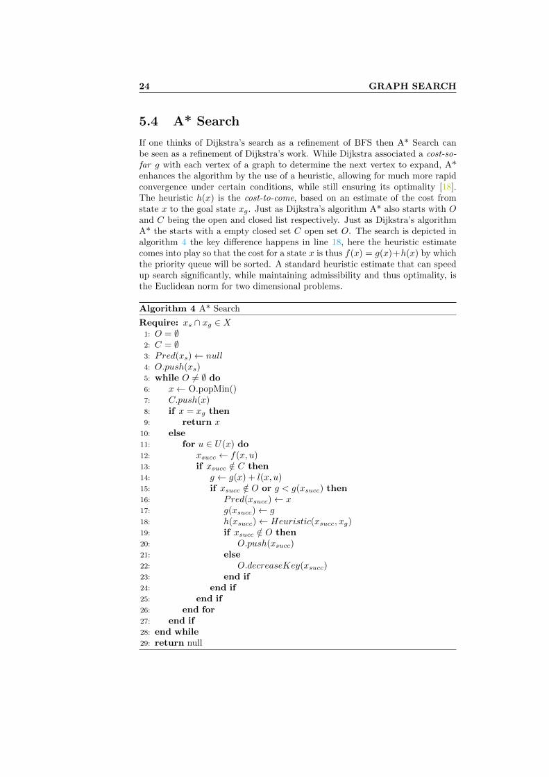
5.4 A* Search

If one thinks of Dijkstra’s search as a refinement of BFS then A* Search canbe seen as a refinement of Dijkstra’s work. While Dijkstra associated a cost-so-far g with each vertex of a graph to determine the next vertex to expand, A*enhances the algorithm by the use of a heuristic, allowing for much more rapidconvergence under certain conditions, while still ensuring its optimality [18].The heuristic h(x) is the cost-to-come, based on an estimate of the cost fromstate x to the goal state xg. Just as Dijkstra’s algorithm A* also starts with Oand C being the open and closed list respectively. Just as Dijkstra’s algorithmA* the starts with a empty closed set C open set O. The search is depicted inalgorithm 4 the key difference happens in line 18, here the heuristic estimatecomes into play so that the cost for a state x is thus f(x) = g(x)+h(x) by whichthe priority queue will be sorted. A standard heuristic estimate that can speedup search significantly, while maintaining admissibility and thus optimality, isthe Euclidean norm for two dimensional problems.

Algorithm 4 A* Search

Require: xs ∩ xg ∈ X1: O = ∅2: C = ∅3: Pred(xs)← null4: O.push(xs)5: while O 6= ∅ do6: x← O.popMin()7: C.push(x)8: if x = xg then9: return x

10: else11: for u ∈ U(x) do12: xsucc ← f(x, u)13: if xsucc /∈ C then14: g ← g(x) + l(x, u)15: if xsucc /∈ O or g < g(xsucc) then16: Pred(xsucc)← x17: g(xsucc)← g18: h(xsucc)← Heuristic(xsucc, xg)19: if xsucc /∈ O then20: O.push(xsucc)21: else22: O.decreaseKey(xsucc)23: end if24: end if25: end if26: end for27: end if28: end while29: return null

5.5 Hybrid A* Search 25

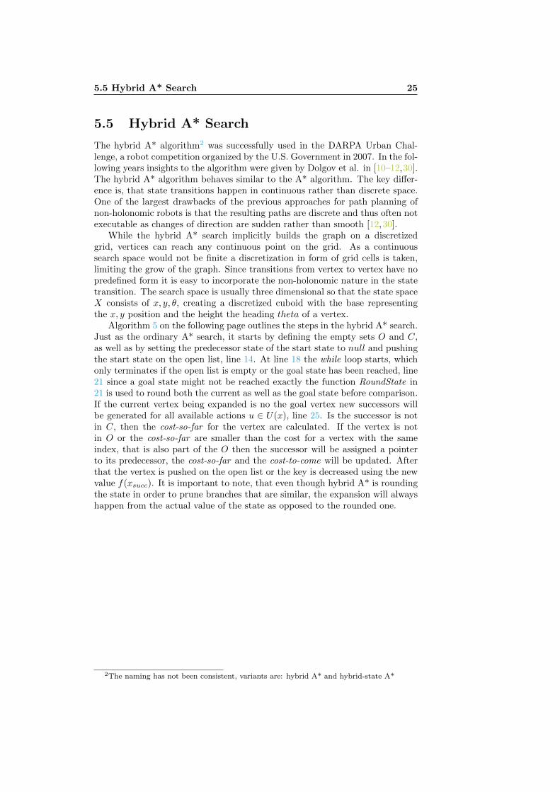
5.5 Hybrid A* Search

The hybrid A* algorithm2 was successfully used in the DARPA Urban Chal-lenge, a robot competition organized by the U.S. Government in 2007. In the fol-lowing years insights to the algorithm were given by Dolgov et al. in [10–12,30].The hybrid A* algorithm behaves similar to the A* algorithm. The key differ-ence is, that state transitions happen in continuous rather than discrete space.One of the largest drawbacks of the previous approaches for path planning ofnon-holonomic robots is that the resulting paths are discrete and thus often notexecutable as changes of direction are sudden rather than smooth [12,30].

While the hybrid A* search implicitly builds the graph on a discretizedgrid, vertices can reach any continuous point on the grid. As a continuoussearch space would not be finite a discretization in form of grid cells is taken,limiting the grow of the graph. Since transitions from vertex to vertex have nopredefined form it is easy to incorporate the non-holonomic nature in the statetransition. The search space is usually three dimensional so that the state spaceX consists of x, y, θ, creating a discretized cuboid with the base representingthe x, y position and the height the heading theta of a vertex.

Algorithm 5 on the following page outlines the steps in the hybrid A* search.Just as the ordinary A* search, it starts by defining the empty sets O and C,as well as by setting the predecessor state of the start state to null and pushingthe start state on the open list, line 14. At line 18 the while loop starts, whichonly terminates if the open list is empty or the goal state has been reached, line21 since a goal state might not be reached exactly the function RoundState in21 is used to round both the current as well as the goal state before comparison.If the current vertex being expanded is no the goal vertex new successors willbe generated for all available actions u ∈ U(x), line 25. Is the successor is notin C, then the cost-so-far for the vertex are calculated. If the vertex is notin O or the cost-so-far are smaller than the cost for a vertex with the sameindex, that is also part of the O then the successor will be assigned a pointerto its predecessor, the cost-so-far and the cost-to-come will be updated. Afterthat the vertex is pushed on the open list or the key is decreased using the newvalue f(xsucc). It is important to note, that even though hybrid A* is roundingthe state in order to prune branches that are similar, the expansion will alwayshappen from the actual value of the state as opposed to the rounded one.

2The naming has not been consistent, variants are: hybrid A* and hybrid-state A*

26 GRAPH SEARCH

Algorithm 5 Hybrid A* Search

1: function roundState(x)2: x.PosX = max{m ∈ Z | m ≤ x.PosX}3: x.PosY = max{m ∈ Z | m ≤ x.PosY }4: x.Angθ = max{m ∈ Z | m ≤ x.Angθ}5: return x6: end function

7: function exists(xsucc,L)8: if {x ∈ L | roundState(x) = roundState(xsucc)} 6= ∅ then9: return true

10: else11: return false12: end if13: end function

Require: xs ∩ xg ∈ X14: O = ∅15: C = ∅16: Pred(xs)← null17: O.push(xs)18: while O 6= ∅ do19: x← O.popMin()20: C.push(x)21: if roundState(x) = roundState(xg) then22: return x23: else24: for u ∈ U(x) do25: xsucc ← f(x, u)26: if ¬exists(xsucc, C) then27: g ← g(x) + l(x, u)28: if ¬exists(xsucc, O) or g < g(xsucc) then29: Pred(xsucc)← x30: g(xsucc)← g31: h(xsucc)← Heuristic(xsucc, xg)32: if ¬exists(xsucc, O) then33: O.push(xsucc)34: else35: O.decreaseKey(xsucc)36: end if37: end if38: end if39: end for40: end if41: end while42: return null

5.5 Hybrid A* Search 27

xg

xs

Dijkstra’s Search A* Search

xg

xs

Figure 5.2: Dijkstra’s Algorithm and A*

Part II

Method, Implementationand Results

Chapter 6

Method

The second part of this thesis presents the hybrid A* method, its implementationas well as simulation results in detail. This chapter will talk about the methodused to solve the navigation problem.

The navigation of a mobile robot in the real as opposed to a discretized world,boils down to a complex, continuous-variable optimization problem. While thereare a great variety of optimal and fast planners for discrete space (Dijkstra, A*),these planners tend to produce solutions that are not suitable for non-holonomicvehicles as they are not smooth and do not incorporate the vehicle constraintsproperly [11]. Using state lattice approaches these issues have been addressed,however this approach comes with the need of precomputing a huge amount ofmotion primitives to account for a multitude of different scenarios and issuesof connecting the lattice appropriately [16, 17, 38]. Other approaches, such asRRT’s, that are especially helpful for finding solutions in higher dimensionalspaces, do produce continuous solutions but inherently come with disadvantagesof being highly nondeterministic and converging towards solutions that are farfrom the optimum and suffer from bug trap problems [20]. The sub-optimalityof RRT’s has been addressed in [20], where a RRT* version that has provenasymptotic optimality is presented. Due to its basic properties, their applicationin path planning is only feasiable with numerous extensions to the original RRT(biasing, heuristics, etc.), Kuwata et al. demonstrated this in [22].

Building on A*, hybrid A* can be seen as the extension of an optimal,deterministic and complete algorithm. Hybrid A* is deterministic and due to theusage of admissible heuristics as well as path smoothing the solutions producedare in the neighborhood of the global optimum. The effective usage of heuristicsdecreases the expansion considerably and lets the search converge towards thesolution quickly.

The hybrid A* planner can be split in three distinct parts. The hybrid A*search that incorporates the vehicles constraints, the heuristics that make thesearch well informed, allowing for fast convergence; and the path smoothingthat improves the found solution using gradient descent.

For the evaluation of the developed algorithm different scenarios presentedin chapter 8 on page 40 are used.

30 METHOD

6.1 Hybrid A* Search

As described in section 5.5 on page 25 the hybrid A* (HA*) search expandsvertices in continuous rather than discrete space. Even though it works incontinuous space, HA* uses a discretized description of the world by pruningsearch branches that have similar leaf states. This is done in order to avoidgrowth of similar branches that add only very little to the solution, but vastlyincrease the size of the search graph.

A state is characterized by x = (x, y, θ), where x and y denote the positionand θ the heading of the vertex respectively. The action set U for a given vertexx can take any shape1. In order to adhere to the constraints imposed by anon-holonomic vehicle, a vertex is expanded by one of three actions; maximumsteering left, maximum steering right as well as no steering. Each of this controlactions is applied for a certain amount of time, resulting in an arc of a circlewith a lower bound turning radius based on the vehicle constraints. This willensure that the resulting paths are always drivable, as the actual vehicle modelis used to expand vertices, even though they might result in excessive steeringactions.

HA* does not take the velocity of the vehicle into account, but based on thesolution of HA* an appropriate velocity profile can easily be calculated.

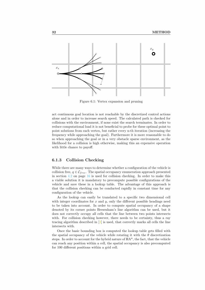
To incorporate the heading of the vehicle a finite three dimensional cuboid,which represents all possible states of the vehicle is used. During the expansionsof vertices with the actions u ∈ U(x) new states are generated. If a new statefalls into a grid cell that is already occupied with another vertex and the newvertex has a lower cost-so-far the old vertex gets pruned (deleted). The searchcontinues until a vertex reaches the goal grid cell, or all reachable cells havebeen reached and thus the open list is empty.

6.1.1 Vertex Expansion and Branch Pruning

The search starts with the current state of the vehicle, denoted as xs. HA*will generate six successor vertices; three driving forward as well as three driv-ing reverse, Figure 6.1 on page 32 depicts the expansion. The successors aregenerated by using arcs with the minimum turning radius of the vehicle2. Thecost for the state transition is based on the length of the arc. Additional costsare accrued for changing driving directions, driving in reverse; and turning, asopposed to going straight. The penalty for turning as well as driving in reverseare multiplicative (depend on portion of the path turning or reversing), whilethe penalty for the change of driving directions is constant.

For each successor the following actions will be executed. If the successorvertex reaches a cell of the three dimensional cuboid that is not part of the closedlist (meaning that cell has not yet been expanded) the evaluation continues. Ifthe cell is not part of the open list (meaning the cell has not been reached priorby any other vertex expansion) or the cost-so-far from the predecessor vertexplus the cost for the vertex expansion to the successor reaching the cell is lower

1An opposing method is to use a state lattice, where a large amount of motion primitivesconnect cells always in a predefined manner.

2The arc length used for the expansion can be chosen arbitrarily, however a shorter lengthpromises higher levels of resolution completeness, as the likelihood to reach each state isincreasing.

6.1 Hybrid A* Search 31

than the cost-so-far of the vertex currently associated with that cell, then thenew vertex will be assigned a pointer to its predecessor, the sum of the cost-so-far from its predecessor plus the cost for the expansion will be assigned to itsg-value and the cost-to-come will be estimated using the heuristics and assignedto its h-value. If the a vertex with the same cell as the successor is on the closedor the open list and the successor’s g-value is not lower, then the successor willbe discarded, the branch will get pruned.

Under the assumption that the steering actions are either maximum steer-ing right, no steering, or maximum steering left the arc length can be simplyexpressed as r

∣∣xθ − x′θ∣∣, r being the minimum turning radius of the vehicle.In case the arc length is shorter than the square root of the cell area, a vertex

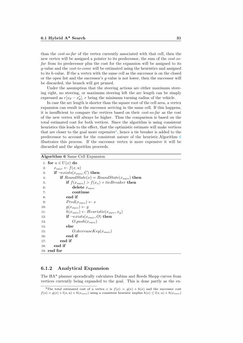
expansion can result in the successor arriving in the same cell. If this happens,it is insufficient to compare the vertices based on their cost-so-far as the costof the new vertex will always be higher. Thus the comparison is based on thetotal estimated cost for both vertices. Since the algorithm is using consistentheuristics this leads to the effect, that the optimistic estimate will make verticesthat are closer to the goal more expensive3, hence a tie breaker is added to thepredecessor to account for the consistent nature of the heuristic.Algorithm 6illustrates this process. If the successor vertex is more expensive it will bediscarded and the algorithm proceeds.

Algorithm 6 Same Cell Expansion

1: for u ∈ U(x) do2: xsucc ← f(x, u)3: if ¬exists(xsucc, C) then4: if RoundState(x) = RoundState(xsucc) then5: if f(xsucc) > f(xx) + tieBreaker then6: delete xsucc7: continue8: end if9: Pred(xsucc)← x

10: g(xsucc)← g11: h(xsucc)← Heuristic(xsucc, xg)12: if ¬exists(xsucc, O) then13: O.push(xsucc)14: else15: O.decreaseKey(xsucc)16: end if17: end if18: end if19: end for

6.1.2 Analytical Expansion

The HA* planner sporadically calculates Dubins and Reeds Shepp curves fromvertices currently being expanded to the goal. This is done partly as the ex-

3The total estimated cost of a vertex x is f(x) = g(x) + h(x) and the successor costf(x) = g(x) + l(x, u) + h(xsucc) using a consistent heuristic implies h(x) ≤ l(x, u) + h(xsucc)

32 METHOD

xg

xs

Figure 6.1: Vertex expansion and pruning

act continuous goal location is not reachable by the discretized control actionsalone and in order to increase search speed. The calculated path is checked forcollisions with the environment, if none exist the search terminates. In order toreduce computational load it is not beneficial to probe for these optimal point topoint solutions from each vertex, but rather every n-th iteration (increasing thefrequency while approaching the goal). Furthermore it is more reasonable to doso when approaching the goal or in a very obstacle sparse environment, as thelikelihood for a collision is high otherwise, making this an expensive operationwith little chance to payoff.

6.1.3 Collision Checking

While there are many ways to determine whether a configuration of the vehicle iscollision free, q ∈ Cfree. The spatial occupancy enumeration approach presentedin section 4.2 on page 16 is used for collision checking. In order to make thisa viable solution it is mandatory to precompute possible configurations of thevehicle and save these in a lookup table. The advantage of this approach isthat the collision checking can be conducted rapidly in constant time for anyconfiguration of the vehicle.

As the lookup can easily be translated to a specific two dimensional cellwith integer coordinates for x and y, only the different possible headings needto be taken into account. In order to compute spatial occupancy of a shapedenoted by its corner points Bresenham’s line algorithm can be used, but itdoes not correctly occupy all cells that the line between two points intersectswith. For collision checking however, there needs to be certainty, thus a raytracing algorithm described in [1] is used, that correctly marks all cells the lineintersects with.

Once the basic bounding box is computed the lookup table gets filled withthe spatial occupancy of the vehicle while rotating it with the θ discretizationsteps. In order to account for the hybrid nature of HA*, the fact, that the vehiclecan reach any position within a cell, the spatial occupancy is also precomputedfor 100 different positions within a grid cell.

6.2 Heuristics 33

6.2 Heuristics

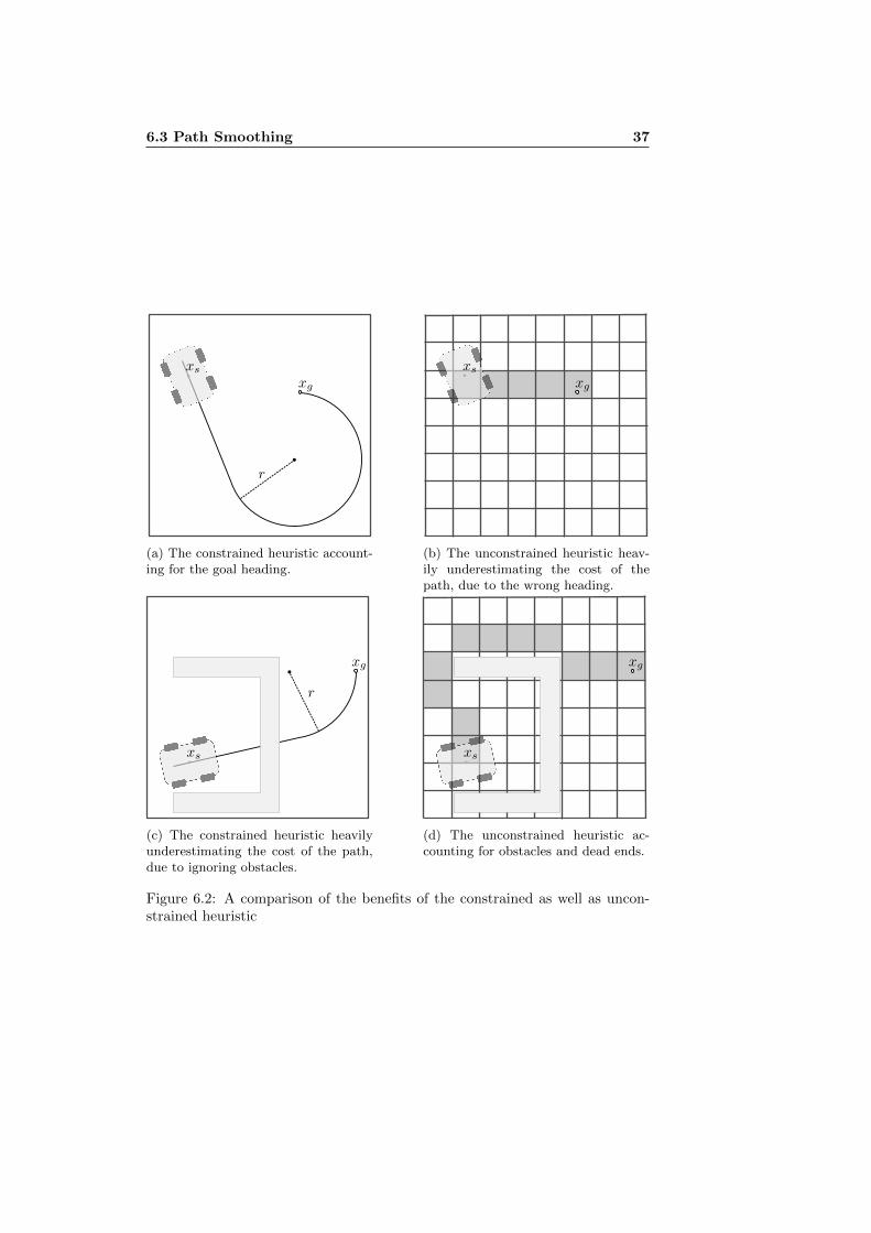
While the goal is to produce drivable solutions that are approaching the opti-mum, it is important to make use of A* being an informed search, implementingheuristics allowing the algorithm converge quickly towards the solution. HA*is using estimates from two heuristics. As both of the heuristics are admissi-ble the maximum of the two is chosen for any given state. The two heuristicscapture very different parts of the problem, which is depicted in Figure 6.2 onpage 37; the constrained heuristic incorporates the restrictions of the vehicle, ig-noring the environment, while the unconstrained heuristic disregards the vehicleconstraints and only accounts for obstacles.

6.2.1 Constrained Heuristic

The constrained heuristic takes the characteristics of the vehicle into account,while neglecting the environment. Suitable candidates are either Dubins orReeds-Shepp curves. These curves introduced in section 3.6 on page 12 are thepaths of minimal length with an upper bound curvature for the forward; andthe forward as well as backward driving car respectively.

Since this heuristic takes the current heading as well as the turning radiusinto account it ensures, that the vehicle approaches the goal with the correctheading. This is especially important, when the car gets closer to the goal. Forperformance reasons this heuristic can be precomputed and stored in a lookuptable. This is possible since it ignores obstacles and hence does not requireany environment information. As it only improves the performance and not thequality of the solution a lookup table has not been implemented.

Given that both Dubins as well as Reeds-Shepp curves are minimal, thisheuristic is clearly admissible.

6.2.2 Unconstrained Heuristic

The unconstrained heuristic neglects the characteristics of the vehicle and onlyaccounts for obstacles. The estimate is based on the shortest distance betweenthe goal node and the vertex currently being expanded. This distance is deter-mined using the standard A* search in two dimensions (x, y position) with anEuclidean distance heuristic. The two dimensional A* search uses the currentvertex as the goal vertex, and the goal vertex of the HA* search as the startvertex. This is beneficial, since the closed list of the A* search stores all shortestdistances g(x) to the goal and can thus be used as a lookup table, instead ofinitiating a new search while HA* progresses.

The unconstrained heuristic guides the vehicle away from dead ends andaround u-shaped obstacles.

Since HA* can reach any point in a cell the unconstrained heuristic needsto be discounted by the absolute difference of the continuous coordinate of thecurrent and the goal vertex.

6.3 Path Smoothing

As the paths produced by the hybrid A* algorithm are drivable, but often aremade up of unnecessary steering actions it is beneficial to post process the result

34 METHOD

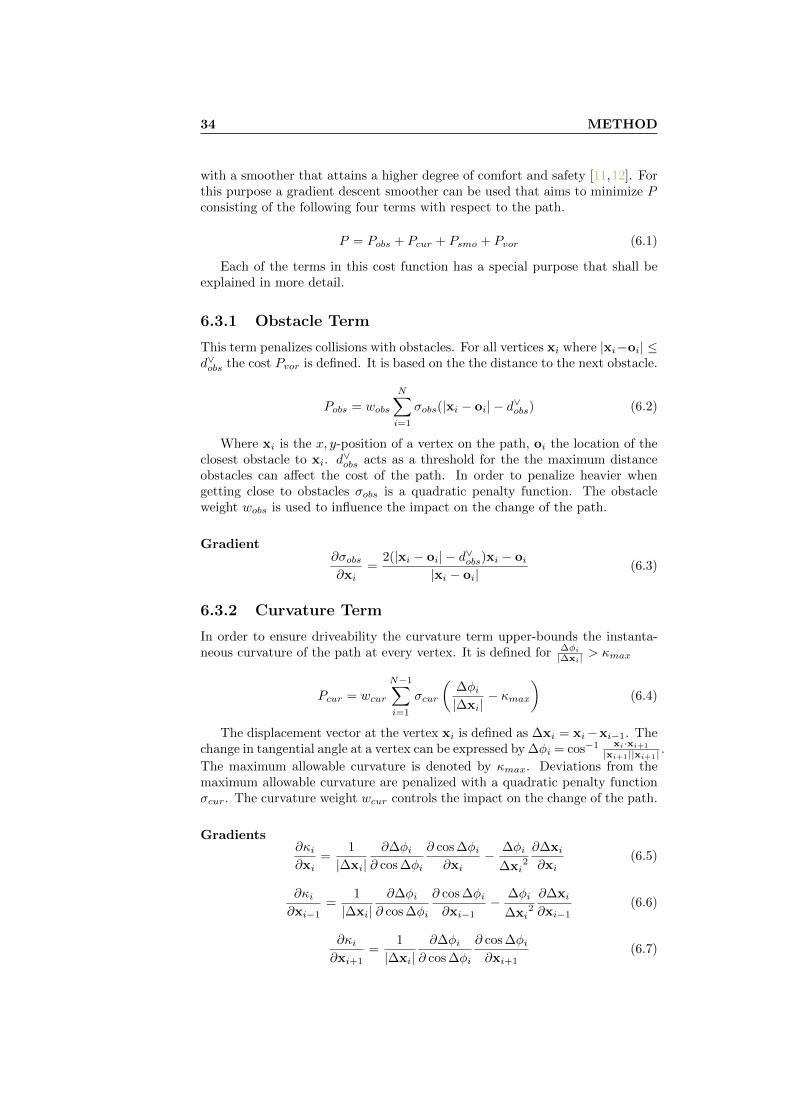
with a smoother that attains a higher degree of comfort and safety [11,12]. Forthis purpose a gradient descent smoother can be used that aims to minimize Pconsisting of the following four terms with respect to the path.

P = Pobs + Pcur + Psmo + Pvor (6.1)

Each of the terms in this cost function has a special purpose that shall beexplained in more detail.

6.3.1 Obstacle Term

This term penalizes collisions with obstacles. For all vertices xi where |xi−oi| ≤d∨obs the cost Pvor is defined. It is based on the the distance to the next obstacle.

Pobs = wobs

N∑i=1

σobs(|xi − oi| − d∨obs) (6.2)

Where xi is the x, y-position of a vertex on the path, oi the location of theclosest obstacle to xi. d∨obs acts as a threshold for the the maximum distanceobstacles can affect the cost of the path. In order to penalize heavier whengetting close to obstacles σobs is a quadratic penalty function. The obstacleweight wobs is used to influence the impact on the change of the path.

Gradient∂σobs∂xi

=2(|xi − oi| − d∨obs)xi − oi

|xi − oi|(6.3)

6.3.2 Curvature Term

In order to ensure driveability the curvature term upper-bounds the instanta-neous curvature of the path at every vertex. It is defined for ∆φi

|∆xi| > κmax

Pcur = wcur

N−1∑i=1

σcur

(∆φi|∆xi|

− κmax)

(6.4)

The displacement vector at the vertex xi is defined as ∆xi = xi−xi−1. Thechange in tangential angle at a vertex can be expressed by ∆φi = cos−1 xi·xi+1

|xi+1||xi+1| .

The maximum allowable curvature is denoted by κmax. Deviations from themaximum allowable curvature are penalized with a quadratic penalty functionσcur. The curvature weight wcur controls the impact on the change of the path.

Gradients∂κi∂xi

=1

|∆xi|∂∆φi

∂ cos ∆φi

∂ cos ∆φi∂xi

− ∆φi

∆xi2

∂∆xi∂xi

(6.5)

∂κi∂xi−1

=1

|∆xi|∂∆φi

∂ cos ∆φi

∂ cos ∆φi∂xi−1

− ∆φi

∆xi2

∂∆xi∂xi−1

(6.6)

∂κi∂xi+1

=1

|∆xi|∂∆φi

∂ cos ∆φi

∂ cos ∆φi∂xi+1

(6.7)

6.3 Path Smoothing 35

6.3.3 Smoothness Term

The smoothness term evaluates the displacement vectors between vertices. Theresult is that it assigns cost to vertices that are unevenly spaced as well aschange direction. wsmo denotes the smoothness weight and hence the impact ofthe term on the change of the path.

Psmo = wsmo

N−1∑i=1

(∆xi+1 −∆xi)2 (6.8)

6.3.4 Voronoi Term

This term guides the path away from obstacles. For dobs ≤ d∨vor the cost Pvoris defined. It is based on the position of the node in the Voronoi field.

Pvor = wvor

N∑i=1

(α

α+ dobs(x, y)

)(dvor(x, y)

dobs + dvor(x, y)

)((dobs(x, y)− d∨vor)2

(d∨vor)2

)(6.9)

The positive distance to the nearest obstacle is denoted by dobs, dedg is thepositive distance to the nearest edge of the GVD. d∨vor represents the maximumdistance obstacles affect the Voronoi potential. α > 0 controls the falloff rate ofthe field and wvor, the Voronoi weight, influences the impact on the path.

Gradients∂dobs∂xi

=xi − oi|xi − oi|

(6.10)

∂dedg∂xi

=xi − ei|xi − ei|

(6.11)

∂ρvor∂dobs

=αdedg

(dobs − d∨vor

) ((dedg + 2d∨vor + α

)dobs +

(d∨vor + 2α

)dedg + αd∨vor

)d∨vor

2 (dobs + α)2 (dobs + dedg

)2(6.12)

∂ρvor∂dedg

=αdobs

(dobs − d∨vor

)2d∨vor

2 (dobs + α)(dedg + dobs

)2 (6.13)

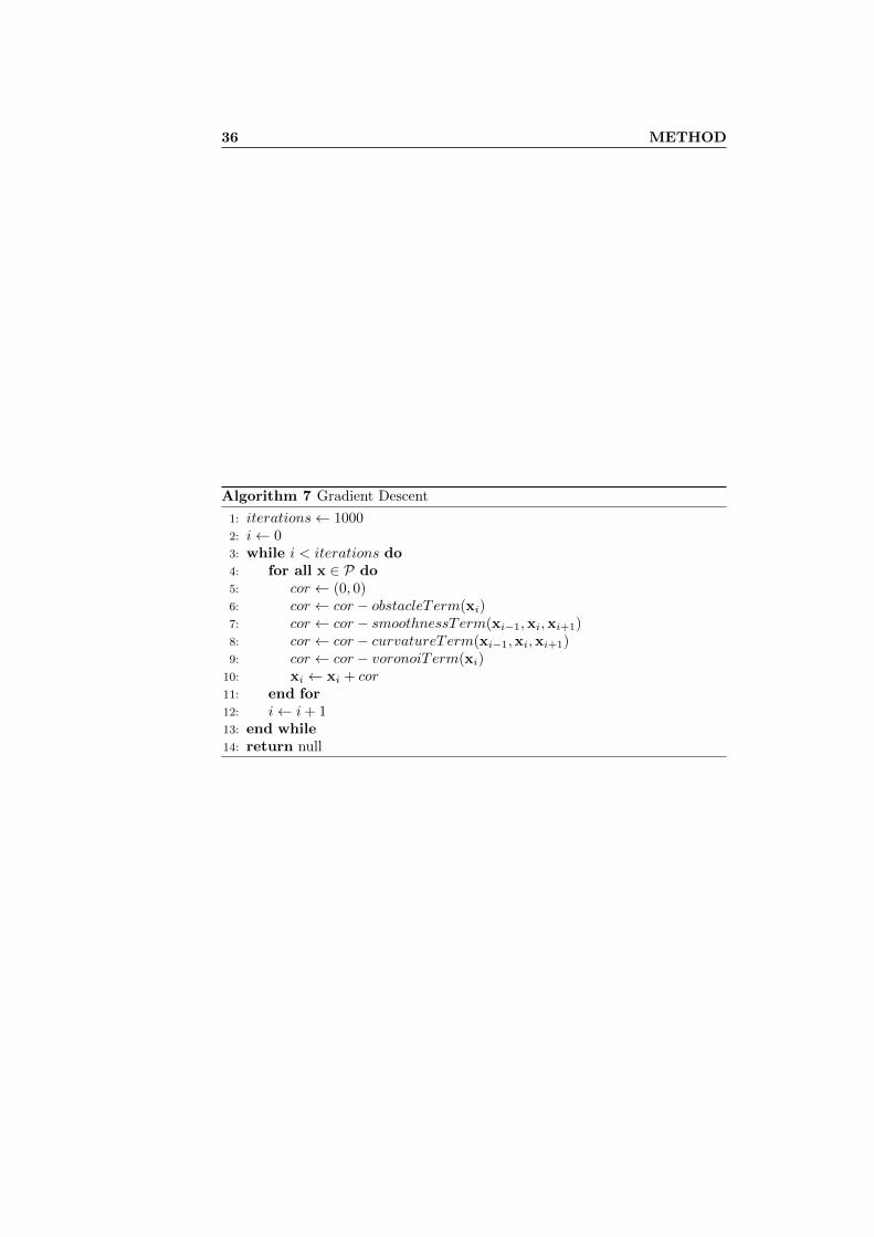
6.3.5 Gradient Descent

The gradient descent method is an optimization algorithm that uses the gradientof the function in order to find a local minimum. Gradient descent progressesstepwise with a step size proportional to the negative gradient of the function,∆x = −∇f(x). While usual implementations use the absolute value of thegradient as a stopping criterion, a fixed number of iterations was chosen toensure run-time consistency. [5]

36 METHOD

Algorithm 7 Gradient Descent

1: iterations← 10002: i← 03: while i < iterations do4: for all x ∈ P do5: cor ← (0, 0)6: cor ← cor − obstacleTerm(xi)7: cor ← cor − smoothnessTerm(xi−1,xi,xi+1)8: cor ← cor − curvatureTerm(xi−1,xi,xi+1)9: cor ← cor − voronoiTerm(xi)

10: xi ← xi + cor11: end for12: i← i+ 113: end while14: return null

6.3 Path Smoothing 37

r

xg

xs

(a) The constrained heuristic account-ing for the goal heading.

xg

xs

(b) The unconstrained heuristic heav-ily underestimating the cost of thepath, due to the wrong heading.

xg

xs

r

(c) The constrained heuristic heavilyunderestimating the cost of the path,due to ignoring obstacles.

xg

xs

(d) The unconstrained heuristic ac-counting for obstacles and dead ends.

Figure 6.2: A comparison of the benefits of the constrained as well as uncon-strained heuristic

Chapter 7

Implementation

The development of the algorithm is conducted in simulation. Since the algo-rithm only requires a binary obstacle grid as an input to compute the output,the poses of the path, the implementation behaves in the same way in simulationas in real driving experiments.

As the path planning algorithm is developed for a real vehicle, the RCV, itdoes require fast computation of paths. The RCV’s top speed is around 12 m/s,the theoretical lower limit of the planner for paths of 30 meters length would thusbe around 2.5 s for a full replanning cycle, avoiding stops due to computation.Since the length is not the only factor that determines the complexity of thesearch a much higher frequency needs to be attained.

The developed hybrid A* planner is able to plan a path from an initial statexs to a final state xg with a frequency of approximately 3–10 Hz1 using mediumgrade consumer hardware (Intel Core i5-5200U 2.2 GHz), making the planner aviable option for real world driving in unstructured environments.

7.1 ROS

The algorithm is wrapped with ROS (Robot Operating System). ROS is chosenas it facilitates the interaction between different modules and hence the deploy-ment in the actual vehicle. At its core, ROS uses a standard messaging system,that allows to publish and listen to different topics between modules that providedifferent functionality, so that the output of one can be easily fed into another.Another benefit of ROS are transforms. Transforms are timestamped coordi-nate frames that automatically conduct necessary coordinate transformationsbetween modules publishing and listening in different coordinate frames.

7.2 Structure

Figure 7.1 on the facing page depicts the structure of the program. The inputsare the obstacle grid as well as the goal pose. During program initializationa collision lookup table as well as a obstacle distance lookup are generated.

1Assuming a 50 m × 100 m grid with a cell size of 1 m and heading discretization of 5◦,which results in 360,000 different possible cells

7.2 Structure 39

Once a occupancy grid and a valid goal pose have been received the hybridA* search begins. To calculate the constrained heuristic Reeds Shepp curvesare calculated. For the unconstrained heuristic a 2D A* search is conducted.In addition to that the algorithm sporadically creates an analytical solutionwith Reeds Shepp curves and if it is collision free terminates and passes thefound path to the smoother. In the smoother the path is optimized for distancebased on closeness to obstacles as well as smoothness, using only the terms Pobsand Psmo due to time constraints and non trivial implementation issues of theVoronoi as well as curvature term. Once the gradient descent terminates thepath is published via ROS to the next module–the controller.

Obstacle Map

qg

Hybrid A* Search

Path Smoothing

Psmooth

Initialization

P

Collision Lookup Distance Map

Reeds Shepp(constrained)

2D A* Search(unconstrained)

Reeds Shepp Solution (analyticalexpansion)

Obstacle Term Smoothness Term

Figure 7.1: Structure of the program with its inputs and outputs

Although the current implementation is useful to conduct experiments with,it can be improved with regard to runtime considerably.

The constrained heuristic can be completely precomputed as it does notaccount for obstacles. For that purpose the Reeds Shepp distance from all cellsin a specified area around the goal to the goal can be saved in a lookup table.

While a lookup table cannot be created before run-time for the unconstrainedheuristic. The two dimensional A* search can be changed in a way, that allowsfor multiple queries. Currently the heuristic stores all closed cells for futurequeries. However, once a cell gets entered by HA* for which the two dimensionalcost are unknown a new A* search from the goal to that cell gets initiated visitingcells that have already been discovered during a previous search.

Chapter 8

Results and Discussion

For the test of the algorithm different scenarios have been chosen and simulationswere conducted to test the efficiency, accuracy and driveability of the solutionsprovided by HA*. The scenarios chosen for the simulation describe commonproblems path planning algorithms need to be able to overcome in order to beusable for the navigation in unstructured environments.

The following scenarios were simulated and are analyzed in the following.Each scenario is different with regard to its obstacle configuration and testsdifferent capabilities. The term Euclidean refers to the use of an unconstrainedEuclidean distance heuristic; 2D A* refers to the unconstrained shortest distanceheuristic, taking obstacles into account; Dubins refers to the constrained shortestDubins curve heuristic, limited to one driving direction; and Reeds Shepp refersto the constrained shortest Reed Shepp curve heuristic allowing for two drivingdirections.

Dark grey areas are free space. Black areas are obstacles. Yellow pathsrepresent the different configurations of the vehicle while traversing the path andare used to visually check paths for collisions. Pink arrows represent a forwardmotion of the vehicle, while purple arrows correspond to a reverse motion. Ifthe path is not accompanied by either pink or purple arrows then the analyticalexpansion has directly connected the most promising current state and the goalstate. Yellow dots represent the area the 2D A* search has visited. A gradientof colors represent the relative cost estimate of each cell among all cells of the2D A* search.

8.1 Simulation Results

8.1.1 Parking Structure

The size of the binary obstacle grid for the parking structure scenario is 50 m× 100 m. The parking structure is horizontally divided by obstacles with twosmall passages connecting both sides. The passages have a width of 4 meters.In the scenario a path needs to be found from the initial state xs (in the lowerhalf), facing north to a final state xg (in the upper half) facing south.

8.1 Simulation Results 41

Analysis

Figure 8.1a on page 45 depicts the planners result using only a Euclidean heuris-tic. It can be seen that the planner finds a non colliding path that is close tothe shortest possible path. The planner has searched the area around the startposition with a bias towards the goal position. The solution path lies in theopposite direction of the search focus.

The found path in Figure 8.1b on page 45 is identical, however the 2D A*heuristic is used. The search progresses away from the goal biased towards thepassage on the left.

Figure 8.1c on page 45 shows the area explored by 2D A* and the colorsrepresent the relative cost of each cell among all explored cells. Red areas areassociated with the highest cost, blue areas with the lowest cost. When lookingat the color gradient it can be seen that the found path follows the gradientvery closely. Only at the beginning, when the vehicle is backing up the costsare increasing.

Discussion

Since the Euclidean heuristic only accounts for relative distance between twopoints and has no information with regard to the obstacles in the environmentit heavily underestimates the cost to the goal and drives the search in the wrongdirection expanding almost one order of magnitude more vertices than the 2DA* heuristic, which gives a clear picture of the environment. Since the 2D A*heuristics is much more informed it underestimates the true cost much less, andhence avoids wasteful expansion of unpromising vertices. The found path inFigure 8.1b on page 45 follows the cost gradient in most parts, but since 2DA* does not account for the non-holonomic nature of the vehicle, it does notaccount for the vehicle’s need to back up out of initial parking position.

8.1.2 Obstacles

The size of the binary obstacle grid for the obstacles scenario is 50 m × 100 m.The environment is randomly scattered with quadratic obstacles of 1 m and 2 mwidth. The initial state xs (left) as well as the goal state xg (right) face west.

Analysis

Figure 8.2a on page 46 shows the path found using the 2D A* heuristic. Thesearch expands vertices in a more or less straight forward manner towards thegoal. In roughly the middle of the grid the analytical expansion finds a solutionand connects collision free to the goal.

Adding the Dubins heuristic in Figure 8.2b on page 46 the search expandsless vertices at the beginning, especially less reversing states. Afterwards thesearch continues towards the goal, but not using the shortest Euclidean path.Much later than 2D A* the search ends due to a successful analytical expansion.

Using the Reeds Shepp heuristic, in Figure 8.2c on page 46 the searchsearches a much larger amount of states in the vicinity of the initial state.While the search progresses towards the goal, it is noticeable that the searchexpands states in a circular fashion along the path, until the analytical expan-sion connects to the goal.

42 RESULTS AND DISCUSSION

Discussion

Since the 2D A* heuristic does not account for the non-holonomic constrains ofthe vehicle it guides the search similar as a Euclidean heuristic would straightto the goal until the Dubins path of the analytical expansion corrects for thebehavior. The Dubins heuristic expands nodes keeping the goal heading of thevehicle in mind, essentially restricting the search to an area along a Dubinscurve. While the heuristic expands much more nodes than the 2D A* only ver-sion, this is due to the fact, that obstacles continuously block a direct connectionfor the path chosen by the Dubins heuristic. Only at last the analytical expan-sion succeeds. For the Reeds Shepp heuristic the case behaves slightly different.Since the heuristic calculates the cost under the assumption that the vehicle candrive in both directions it allows for much more reverse states to be expanded.Along the path towards the goal the Reeds Shepp heuristic continuously tries tochange the heading of the car by expanding states that deviate from the pathin a circular fashion.

8.1.3 Wall

The size of the binary obstacle grid for the wall scenario is 50 m × 100 m. Theenvironment consits of a wall obstacle of 6 m width. The initial state xs (left)faces east and the goal state xg (right) faces north.

Analysis

Figure 8.3 on page 47 shows the path found using the Euclidean heuristic.The search progresses in a straight line towards the wall, until the analyticalexpansion finds a non colliding solution.

Using the 2D A* heuristic in Figure 8.3b on page 47 the search is biased tothe area above the wall. The path connects with an analytical expansion.

Figure 8.3c on page 47 shows the resulting path using the Reeds Sheppheuristic. The search progresses early on to the area below the wall until theanalytical expansion finds an appropriate solution.

Discussion

Since the Euclidean heuristic is oblivious to the wall, the search progressesstraight towards the goal. Due to the analytical expansion the search ends earlyotherwise the search would have expanded cells that are located in the area topof the wall and possibly connected via a Reeds Shepp path instead of a Dubins.In the second figure, the 2D A* heuristic does account for the wall, but does notmodel the non-holonomic constraints appropriately, hence the search diverges tothe wrong direction increasing the path length unnecessarily. The Reeds Sheppheuristic on the other hand, even though not aware of the wall, incorporatesthe non-holonomic characteristics and tries to approach the goal with the rightheading from the start, leading to an overall much shorter path.

8.1.4 Dead End

The size of the binary obstacle grid for the dead end scenario is 50 m × 100 m.The environment consist of a large u-shaped obstacle. The initial state xs (left)

8.1 Simulation Results 43

faces east, while the goal state xg (right) faces north.

Analysis

Figure 8.4 on page 48 shows the path found using the Euclidean heuristic. Thesearch expands a large amount of the available cells and searches the inner partof the u-shaped obstacle before it searches outside of the same. Shortly beforethe search reaches the goal the analytical expansion completes the path.

The 2D A* heuristic in Figure 8.4b on page 48 barely searches the inner partof the obstacle. It quickly searches around it and creates a solution passing thelower part and then converging straight towards the goal, until the analyticalexpansion completes the path.

Adding the Reeds Shepp heuristic in Figure 8.3c on page 47 the searchexpands much less cells in the area above and below the obstacle and eventuallyconnects via analytical expansion.

Discussion

A u-shaped obstacle or dead end is a tough hurdle to take for the Euclideanheuristic that is not aware of its surroundings. The Euclidean heuristic heav-ily underestimates the cost and gets stuck inside the obstacle until the costof the solutions so far increase to a level that justifies the detour below theobstacle. While the resulting path is approaching the optimal the number ofvertices expanded is unacceptable for a real-time implementation. Using the2D A* heuristic the problem gets circumvented as it is aware of the dead endahead. The solution quickly converges towards the goal around the obstacle.However as 2D A* does not take the heading into account the angle at which itapproaches the goal is inadequate for a good analytical expansion; the result isan unnecessary circle for the correction of the heading. Taking the heading intoaccount, the addition of the Reeds Shepp heuristic further reduces the numberof vertices expanded, and thus considered optimal. While the analytical expan-sion finds a solution prior to leaving the obstacle behind Reeds Shepp wouldhave approached the obstacle in the right way either way.

8.1.5 Additional Simulations

In order to test the HA* planner for turning as well as parking maneuvers twoadditional simulations are conducted.

Analysis

Figure 8.5 on page 49 shows HA* finding a path in a 5 m wide alley allowingthe vehicle to change heading by 180 degrees. The turning is conducted in astar shape, where the vehicle reverses with the maximum steering angle right,changes to the maximum steering angle left and drives forward and repeats theprocess. For the parallel parking case a similar behavior can be observed asdepicted by Figure 8.6 on page 49.

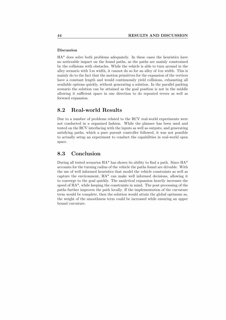
44 RESULTS AND DISCUSSION

Discussion

HA* does solve both problems adequately. In these cases the heuristics haveno noticeable impact on the found paths, as the paths are mainly constrainedby the collisions with obstacles. While the vehicle is able to turn around in thealley scenario with 5 m width, it cannot do so for an alley of 4 m width. This ismainly do to the fact that the motion primitives for the expansion of the verticeshave a constant length and would continuously yield collisions, exhausting allavailable options quickly, without generating a solution. In the parallel parkingscenario the solution can be attained as the goal position is not in the middleallowing it sufficient space in one direction to do repeated revers as well asforward expansion.

8.2 Real-world Results

Due to a number of problems related to the RCV real-world experiments werenot conducted in a organized fashion. While the planner has been used andtested on the RCV interfacing with the inputs as well as outputs, and generatingsatisfying paths, which a pure pursuit controller followed, it was not possibleto actually setup an experiment to conduct the capabilities in real-world openspace.

8.3 Conclusion

During all tested scenarios HA* has shown its ability to find a path. Since HA*accounts for the turning radius of the vehicle the paths found are drivable. Withthe use of well informed heuristics that model the vehicle constraints as well ascapture the environment, HA* can make well informed decisions, allowing itto converge to the goal quickly. The analytical expansion heavily increases thespeed of HA*, while keeping the constraints in mind. The post processing of thepaths further improves the path locally. If the implementation of the curvatureterm would be complete, then the solution would attain the global optimum as,the weight of the smoothness term could be increased while ensuring an upperbound curvature.

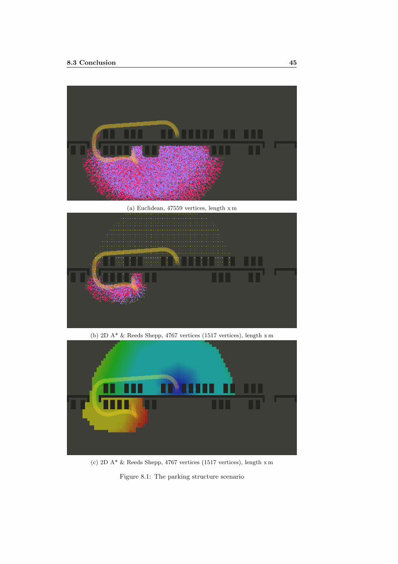
8.3 Conclusion 45

(a) Euclidean, 47559 vertices, length xm

(b) 2D A* & Reeds Shepp, 4767 vertices (1517 vertices), length xm

(c) 2D A* & Reeds Shepp, 4767 vertices (1517 vertices), length xm

Figure 8.1: The parking structure scenario

46 RESULTS AND DISCUSSION

(a) 2D A*, 2685 vertices, length 116.882m

(b) 2D A* & Dubins, 3486 vertices, length 114.961m

(c) 2D A* & Reeds Shepp, 4316 vertices, length 116.647m

Figure 8.2: The obstacle scenario

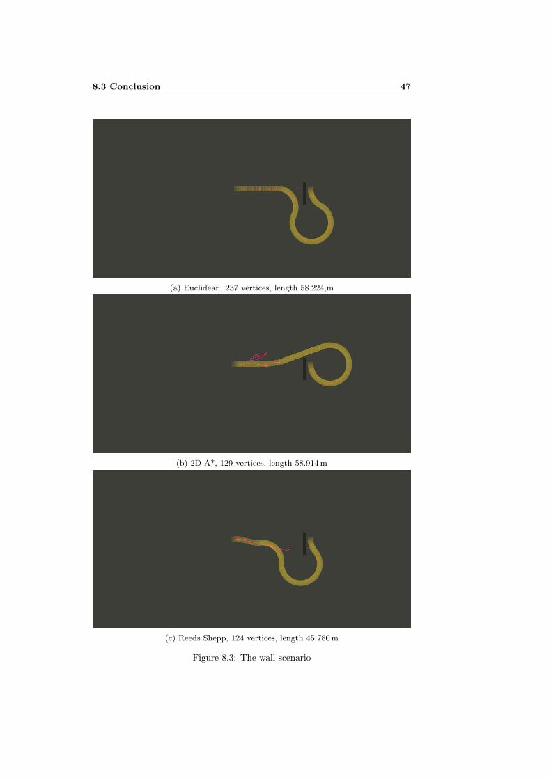
8.3 Conclusion 47

(a) Euclidean, 237 vertices, length 58.224,m

(b) 2D A*, 129 vertices, length 58.914m

(c) Reeds Shepp, 124 vertices, length 45.780m

Figure 8.3: The wall scenario

48 RESULTS AND DISCUSSION

(a) Euclidean, 72014 vertices, length 90.0001m

(b) 2D A*, 8871 vertices, length 128.197m

(c) 2D A* & Reeds Shepp, 8691 vertices, length 90.9778m

Figure 8.4: The dead end scenario

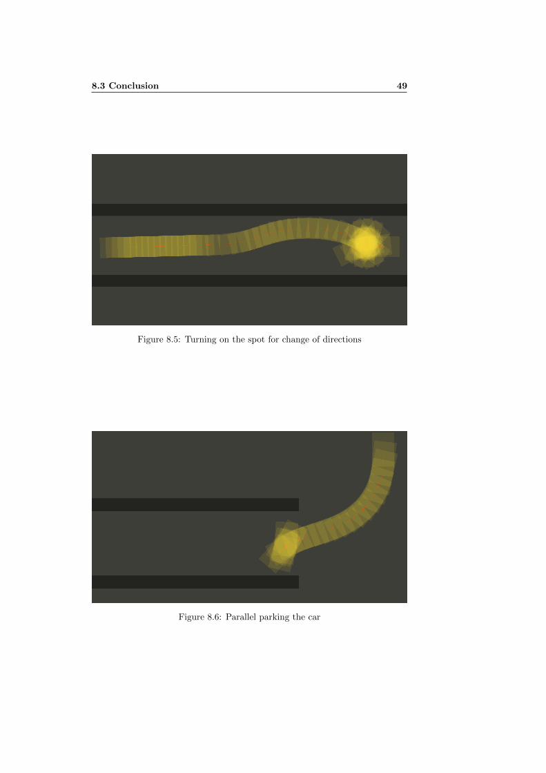
8.3 Conclusion 49

Figure 8.5: Turning on the spot for change of directions

Figure 8.6: Parallel parking the car

Chapter 9

Conclusion

While the research in the area of autonomous driving continuous to grow, theDARPA Grand Challenge and especially the Urban Challenge have marked im-portant milestones, greatly propelling the development. Hence it is not aston-ishing that companies heavily engaged in autonomous driving, such as Alphabet(formerly Google) or Uber recruited a large part of past participants of thesechallenges.

Since there are many ways to solve navigation problems of this kind thechoice might seem arbitrary. While the team from CMU and winner of the DUCused a lattice planner with D* [16,28], the MIT team used an heavily modifiedversion of RRT both for structured as well as unstructured driving [22].

The hybrid A* algorithm is yet another approach. It is a fast planner usedfor planning in unstructured environments by the Standford team, developedby Dolgov, Thrun, Montemerlo (Google Self-Driving Cars), Diebel (Cedar LakeVentures), participating with Junior in the DUC. This thesis has analyzed HA*thoroughly and developed a similar version for the KTH RCV in C++ and ROS.

The resulting hybrid A* planner addresses the problem of finding a solutionto the problem described in section 1.3 on page 3 properly. The planner modelsthe non-holonomic nature of the vehicle in all stages of the process, vertexexpansion, heuristic estimates, as well as analytic expansion. Thus, the mostimportant characteristic of the paths is given–they are driveable.

The HA* planner solves a challenging problem in an elegant manner. HA*is fast, as it reduces the search space with the help of well informed heuristics,allowing it to converge to the goal quickly. Based on the initial solution thelocal smoothing attains a solution approaching the global optimum. Ideal sce-narios for the planner are slow speed driving in unstructured environments. Anexample of that might be navigating parking lots as well as automated parkingand valet parking.

The source code for this project is publicly available and can be found here,https://github.com/karlkurzer/path_planner; an additional documenta-tion can be found here http://karlkurzer.github.io/path_planner.

Chapter 10

Future Work

While the algorithm developed in this thesis has already been successfully testedon the RCV there are still aspects that are reasonable to consider and wouldeither improve the search speed or the quality of the overall solution. In thefollowing the most promising improvements are shortly presented.

10.1 Variable Resolution Search

HA* uses a constant cell size and constant arc length for the vertex expansion.Usually it is desirable to increase the resolution as much as computationallypossible. This will ensure greater notions of completeness as well as optimality.Completeness will be improved since a coarse resolution underestimates the freespace Cfree, making narrow passages appear not traversable without collision.A higher resolution will also create solutions that are closer to the optimum, asopposed to coarse resolutions where the solution oscillates around the optimum.In terms of computational efficiency a variable resolution search can greatlyreduce the expansions necessary to converge towards the goal.

The two possibilities to make improvements in the areas of completeness aswell as computational efficiency are either locally changing the arc length for thevertex expansion or the resolution of the cells. While locally changing the cellresolution requires a different data structure representing the cells it is easierto increase the arc length used for the vertex expansion. The arc length can bebased on the size of the free space it expands to. A convenient representationof this can be achieved using the Voronoi diagram.

10.2 Heuristic Lookup Table

During the HA* search the constrained heuristic constantly evaluates the short-est distance from the vehicles current configuration to the goal configurationunder the assumption that no obstacles exists and the car is constrained bya lower bound turning radius. As this heuristic is not dependent on sensorinformation it can be completely precomputed and retrieved during run-time.

52 FUTURE WORK

10.3 Velocity Profile Generation

A reasonable addition to the HA* planner is the calculation of a velocity profile.Based on the smoothed path a reference velocity could be calculated in differentways. A simple approach would be an upper bound lateral acceleration ay of thevehicle based on the curvature of each segment of the path. For more insightswith regard to the lateral dynamics of the path at given velocities a linear singletrack model can then be simulated along the path.

10.4 Path Commitment and Replanning

As the vehicle is progressing towards the goal the sensors will detect new ob-stacles in the environment that have previously been out of range or covered byother obstacles. In order to incorporate possible changes in the environment inthe path planning HA* recomputes the path to the goal with every update ofthe environment it receives.

This is often not necessary. Given the fact, that the sensor information in thevicinity of the car is of high quality replanning, if at all, does not need to start atthe vehicles current position. A path commitment can significantly reduce theplanning effort. Commitment to the path means that as new sensor informationarrives the path will not be replanned at the vehicle’s current position, but ratherat the n-th vertex that is still in an area where the sensors reliably perceive theenvironment.

As planning an entire path takes considerably more time than merely check-ing the same for collisions one has to ask, whether it is feasible to replan a pathas opposed to just check the current path for collisions given the updated modelof the environment.

Another aspect are dynamic obstacles that temporarily collide with the path.The current version of HA* cannot distinguish between dynamic and staticobstacles, as a dynamic obstacle, like a static obstacles, only leaves a binaryfootprint on the occupancy grid. This will leave the planner to believe thatreplanning is the right way to solve this problem. While for the static case itwould be reasonable to replan based on the new information it is undesirablefor dynamic obstacles since the planner does not account for the velocity of theobstacle and hence does not guarantee the path being safe.

Bibliography

[1] John Amanatides, Andrew Woo, et al. A fast voxel traversal algorithm forray tracing. 32

[2] Richard Bellman. Dynamic programming. Dover Publications, Mineola,N.Y., dover ed. edition, 2003. 20

[3] Michele Bertoncello and Dominik Wee. Ten ways autonomous driving couldredefine the automotive world, 2015. 3

[4] Bela Bollobas. Fundamentals, 1979. 18

[5] Stephen P. Boyd and Lieven Vandenberghe. Convex optimization. Cam-bridge University Press, Cambridge, 2004. 35

[6] Rodney A. Brooks and Tomas Lozano-Perez. A subdivision algorithm inconfiguration space for findpath with rotation. IEEE Transactions on Sys-tems, Man, and Cybernetics, SMC-15(2):224–233, 1985. 11

[7] B. Chazelle and D. P. Dobkin. Intersection of convex objects in two andthree dimensions. Journal of the ACM (JACM), 34(1):1–27, 1987. 15

[8] Thomas H. Cormen. Introduction to algorithms. MIT Press, Cambridge,Mass., 3rd ed. edition, 2009. 21, 22

[9] E. W. Dijkstra. A note on two problems in connexion with graphs. Nu-merische Mathematik, 1(1):269–271, 1959. 22

[10] Dmitri Dolgov and Sebastian Thrun. Autonomous driving in semi-structured environments: Mapping and planning. pages 3407–3414, 2009.25

[11] Dmitri Dolgov, Sebastian Thrun, Michael Montemerlo, and James Diebel.Practical search techniques in path planning for autonomous driving. 2008.25, 29, 34

[12] Dmitri Dolgov, Sebastian Thrun, Michael Montemerlo, and James Diebel.Path planning for autonomous vehicles in unknown semi-structured envi-ronments. The International Journal of Robotics Research, 29(5):485–501,2010. 25, 34

[13] L. E. Dubins. On curves of minimal length with a constraint on averagecurvature, and with prescribed initial and terminal positions and tangents.American Journal of Mathematics, 79(3):497, 1957. 13

54 BIBLIOGRAPHY

[14] Christer Ericson. Real-time collision detection. Morgan Kaufmann seriesin interactive 3D technology. Elsevier, Amsterdam and London, 2005. 15,16, 17

[15] Ariel Felner. Position paper: Dijkstra’s algorithm versus uniform costsearch or a case against dijkstra’s algorithm. 2011. 22

[16] Dave Ferguson, Thomas M. Howard, and Maxim Likhachev. Motion plan-ning in urban environments part i. pages 1063–1069, 2008. 29, 50

[17] Dave Ferguson, Thomas M. Howard, and Maxim Likhachev. Motion plan-ning in urban environments part ii. pages 1070–1076, 2008. 29

[18] Peter E. Hart, Nils J. Nilsson, and Bertram Raphael. A formal basis forthe heuristic determination of minimum cost paths. IEEE Transactions onSystems Science and Cybernetics, 4(2):100–107, 1968. 20, 21, 24

[19] V. Hayward. Fast collision detection scheme by recursive decomposition ofa manipulator workspace, 1986. 16, 17

[20] S. Karaman and E. Frazzoli. Incremental sampling-based algorithms foroptimal motion planning. In Yoky Matsuoka, Hugh F. Durrant-Whyte,and Jose Neira, editors, Robotics, volume 06, Cambridge, MA, 2011. MITPress. 29

[21] O. Khatib. Real-time obstacle avoidance for manipulators and mobilerobots. The International Journal of Robotics Research, 5(1):90–98, 1986.10

[22] Yoshiaki Kuwata, Gaston A. Fiore, Justin Teo, Emilio Frazzoli, andJonathan P. How. Motion planning for urban driving using rrt. 2008.29, 50

[23] Jean-Claude Latombe. Robot Motion Planning, volume 124 of The SpringerInternational Series in Engineering and Computer Science, Robotics: Vi-sion, Manipulation and Sensors. Springer US, Boston, MA, 1991. 7, 8, 9,11, 12

[24] S. M. Lavalle. Rapidly-exploring random trees: a new tool for path plan-ning. 1998. 10

[25] S. M. Lavalle and J. J. Kuffner. Randomized kinodynamic planning. 1:473–479 vol.1, 1999. 10

[26] Steven Michael LaValle. Planning algorithms. Cambridge University Press,Cambridge, 2006. 7, 8, 9, 11, 12, 15, 16, 19, 20, 21, 22

[27] C. Y. Lee. An algorithm for path connections and its applications. IRETransactions on Electronic Computers, EC-10(3):346–365, 1961. 21

[28] Maxim Likhachev, Dave Ferguson, Geoff Gordon, Anthony Stentz, andSebastian Thrun. Anytime dynamic a*: An anytime, replanning algorithm.50

BIBLIOGRAPHY 55

[29] T. Lozano-Perez. Spatial planning: A configuration space approach. IEEETransactions on Computers, C-32(2):108–120, 1983. 8

[30] Michael Montemerlo, Jan Becker, Suhrid Bhat, Hendrik Dahlkamp, DmitriDolgov, Scott Ettinger, Dirk Haehnel, Tim Hilden, Gabe Hoffmann,Burkhard Huhnke, Doug Johnston, Stefan Klumpp, Dirk Langer, AnthonyLevandowski, Jesse Levinson, Julien Marcil, David Orenstein, JohannesPaefgen, Isaac Penny, Anna Petrovskaya, Mike Pflueger, Ganymed Stanek,David Stavens, Antone Vogt, and Sebastian Thrun. Junior: The stanfordentry in the urban challenge. Journal of Field Robotics, 25(9):569–597,2008. 25

[31] Xavier Mosquet, Thomas Dauner, Nikolaus Lang, Michael Russmann, An-tonella Mei-Pochtler, Rakshit Agrawal, and Florian Schmieg. Revolutionin the driver’s seat: The road to autonomous vehicles. 3

[32] Allen Newell and Herbert A. Simon. Computer science as empirical inquiry:symbols and search. Communications of the ACM, 19(3):113–126, 1976. 20

[33] M. K. Ponamgi, D. Manocha, and M. C. Lin. Incremental algorithmsfor collision detection between polygonal models. IEEE Transactions onVisualization and Computer Graphics, 3(1):51–64, 1997. 15

[34] J. A. Reeds and L. A. Shepp. Optimal paths for a car that goes bothforwards and backwards. Pacific Journal of Mathematics, 145(2):367–393,1990. 14

[35] Stuart J. Russell, Peter Norvig, and Ernest Davis. Artificial intelligence:A modern approach. Prentice Hall series in artificial intelligence. PrenticeHall, Upper Saddle River, 3rd ed. edition, 2010. 21

[36] Steven S. Skiena. The algorithm design manual. Springer, London, 2nd ed.edition, 2008. 19, 21

[37] C. Urmson and R. Simmons. Approaches for heuristically biasing rrtgrowth, 2003. 10

[38] Chris Urmson, Joshua Anhalt, Drew Bagnell, Christopher Baker, RobertBittner, M. N. Clark, John Dolan, Dave Duggins, Tugrul Galatali, ChrisGeyer, Michele Gittleman, Sam Harbaugh, Martial Hebert, Thomas M.Howard, Sascha Kolski, Alonzo Kelly, Maxim Likhachev, Matt Mc-Naughton, Nick Miller, Kevin Peterson, Brian Pilnick, Raj Rajkumar, PaulRybski, Bryan Salesky, Young-Woo Seo, Sanjiv Singh, Jarrod Snider, An-thony Stentz, William “Red” Whittaker, Ziv Wolkowicki, Jason Ziglar,Hong Bae, Thomas Brown, Daniel Demitrish, Bakhtiar Litkouhi, Jim Nick-olaou, Varsha Sadekar, Wende Zhang, Joshua Struble, Michael Taylor,Michael Darms, and Dave Ferguson. Autonomous driving in urban en-vironments: Boss and the urban challenge. Journal of Field Robotics,25(8):425–466, 2008. 2, 29

[39] Jens Ziegler, Moritz Werling, and Jochen Schroder. Navigating car-likerobots in unstructured environments using an obstacle sensitive cost func-tion. IEEE, 2008. 17

TRITA -AVE 2016:41

ISSN 1651-7660

www.kth.se