Path Estimation from GPS Tracks

Chris Brunsdon

Department of GeographyUniversity of Leicester

University Road, Leicester LE1 7RUTelephone: +44 116 252 3843

Fax: +44 116 252 3854Email: cb179@le.ac.uk

1. IntroductionThe widespread availability of hand-held GPS units has led to a proliferation in data on the tracksof individuals as they walk, drive or otherwise go about journeys. This data has been used ina number of ways - for example the OpenStreetMap project (The OpenStreetMap Foundation2007). One characteristic of projects such as this is that there will often be several GPS tracks forthe same stretch of road. In general, repeatedly measuring something and taking the average ofmeasurements leads to a more accurate result. The question addressed here is “is it possible to’average’ GPS tracks and if so, does this lead to a better estimate of road location?”.

2. Tracing Paths From GPS DataIn this section, the key technique for identifying paths from GPS data will be introduced. Thisapproach is called Principal Curve Analysis (Hastie and Stuetzle 1989). Here, the basic principalcurve algorithm will be used, as well as some proposed modifications to address specific issuesrelating to the estimation of cartographic data.

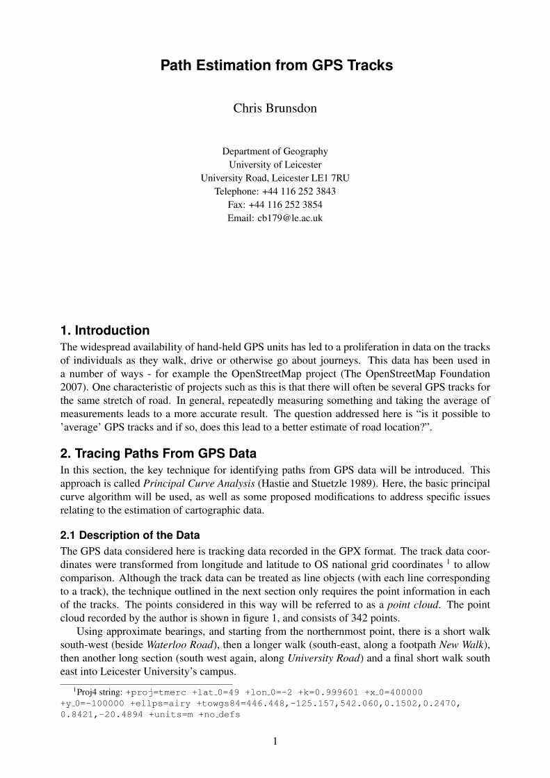
2.1 Description of the DataThe GPS data considered here is tracking data recorded in the GPX format. The track data coor-dinates were transformed from longitude and latitude to OS national grid coordinates 1 to allowcomparison. Although the track data can be treated as line objects (with each line correspondingto a track), the technique outlined in the next section only requires the point information in eachof the tracks. The points considered in this way will be referred to as a point cloud. The pointcloud recorded by the author is shown in figure 1, and consists of 342 points.

Using approximate bearings, and starting from the northernmost point, there is a short walksouth-west (beside Waterloo Road), then a longer walk (south-east, along a footpath New Walk),then another long section (south west again, along University Road) and a final short walk southeast into Leicester University’s campus.

1Proj4 string: +proj=tmerc +lat 0=49 +lon 0=-2 +k=0.999601 +x 0=400000+y 0=-100000 +ellps=airy +towgs84=446.448,-125.157,542.060,0.1502,0.2470,0.8421,-20.4894 +units=m +no defs

1

© C

row

n C

opyr

ight

/dat

abas

e rig

ht 2

007.

An

Ord

nanc

e S

urve

y/E

DIN

A s

uppl

ied

serv

ice

Nor

th −

>

Scale: 200m

Figure 1: A point cloud showing recorded GPS tracks in Leicester.

2

2.2 Principal Curve AnalysisThe idea here is to find a curve running through the ’middle’ of the point cloud. One way ofdefining the ’middle curve’ is to say that it is the curve minimising the total squared distancesto each point in the point cloud. If we consider the point cloud to be a list of n coordinate pairs{pi = (xi, yi) : i = 1, n}, and our curve as a parametrised curve f(λ) = (fx(λ), fy(λ)), then thedistance between pi and f is the closest point to pi on f :

D(pi, f) = argminλ||pi − f(λ)|| (1)

and the ’middle’ curve f̂ mimimises the expression∑

i D2(f ,pi). Curves satisfying these require-ments are known as principal curves. It is noted that the parametrisation of f is not unique — f(λ)could be replaced by f(g(λ)) where g(.) is any monotone function. To resolve this ambiguity, itis specified that λ should be the distance travelled along the curve f — in this case, λ is thereforethe distance travelled along the ’middle curve’ of the GPS point cloud.

In order to estimate f (Hastie and Stuetzle 1989) attempt to reconstruct the curve at a numberof discrete points {f(λi) : i = 1...n} where i corresponds to the index for the points in the pointcloud. Given an initial guess at f , the curve is reconstructed using the following method:

1. Find the nearest points to each pi on the guessed curve, and compute the distance along thecurve to each point. This provides a set of estimates for the λi’s

2. The estimate of f is then updated by updating estimates for the two functions fx(λ), fy(λ)using a non-parametric smooth regression procedure (such as Cleveland (1979) or Greenand Silverman (1994)) applied respectively to the (λi, xi) and (λi, yi) pairs.

3. Return to step 1 with the updated estimate of f

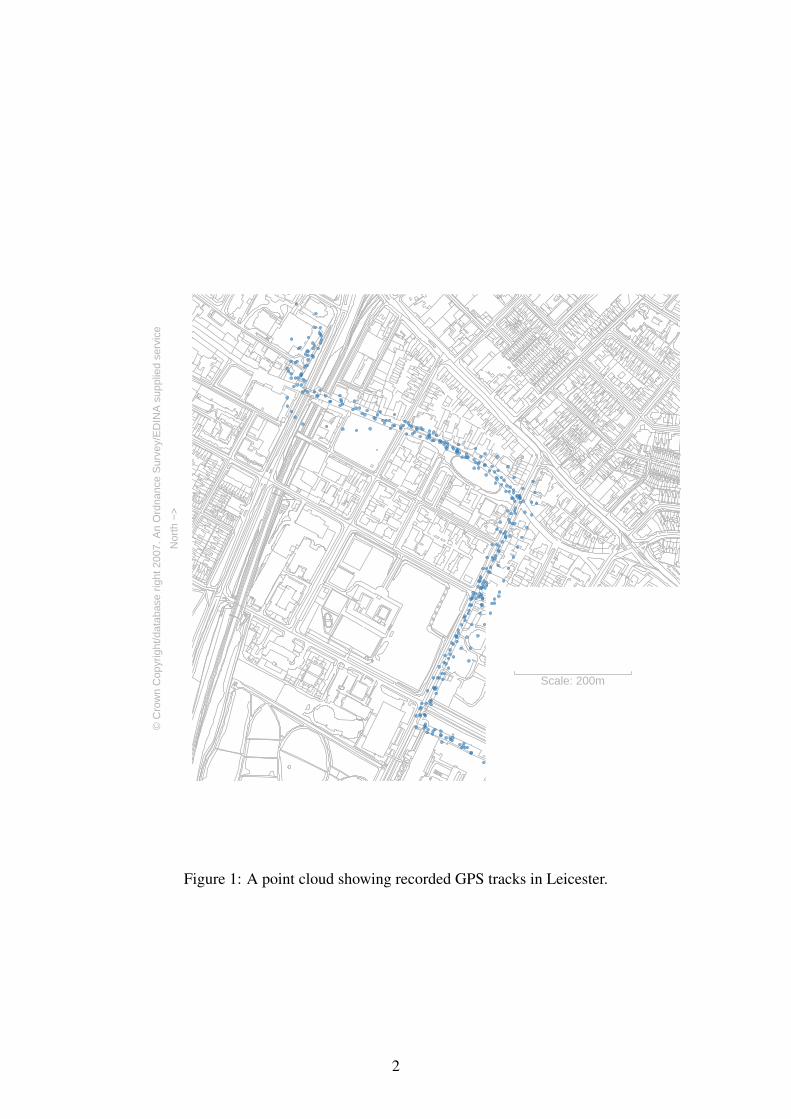
The result of applying the algorithm to the point cloud data used here is shown in figure 2. Theprincipal curve is shown in red - the black lines correspond to the distances of each individual pointin the cloud to the line. Note a key difference between this technique and standard non-parametricregression — here the distances to be minimised can be in any direction, depending on the linejoining a GPS point and the closest point to it on the principal curve, while in standard regressiontechniques, distances are always measured in the same direction — parallel to the y-axis

2.3 Adapting the AlgorithmFigure 2 demonstrates the general accuracy of the principal curve algorithm, but also highlightsone of its pitfalls. At times GPS tracks can exhibit systematic errors - at the north end of NewWalk, there is clearly a rogue track which veers noticeably from the true location - it may beseen as a ‘dog leg’ swinging away from New Walk, apparently crossing the railway line havingpassed through some buildings. This means that although in most places the curve provides agood estimate of the road or pathway, it swings out in locations near to the rogue track.

A way of overcoming this is to devise a robust variant on the principal curve algorithm - theapproach is outlined below:

1. Fit a principal curve using the standard approach.

2. Note the distances from each point to the curve - call these {di}

3. Standardise these distances by dividing by their standard deviation - call these {d∗i }.

4. Compute a set of weights as a monotone decreasing function of the d∗i ’s - typically let wi = 1if d∗i < 3, wi = 4 − d∗i if 3 < d∗i < 4 and wi = 0 if d∗i > 4.

3

© C

row

n C

opyr

ight

/dat

abas

e rig

ht 2

007.

An

Ord

nanc

e S

urve

y/E

DIN

A s

uppl

ied

serv

ice

Nor

th −

>

Scale: 200m

Figure 2: Principal curve (red) fitted to GPS point cloud data.

4

© C

row

n C

opyr

ight

/dat

abas

e rig

ht 2

007.

An

Ord

nanc

e S

urve

y/E

DIN

A s

uppl

ied

serv

ice

Nor

th −

>

Scale: 200m

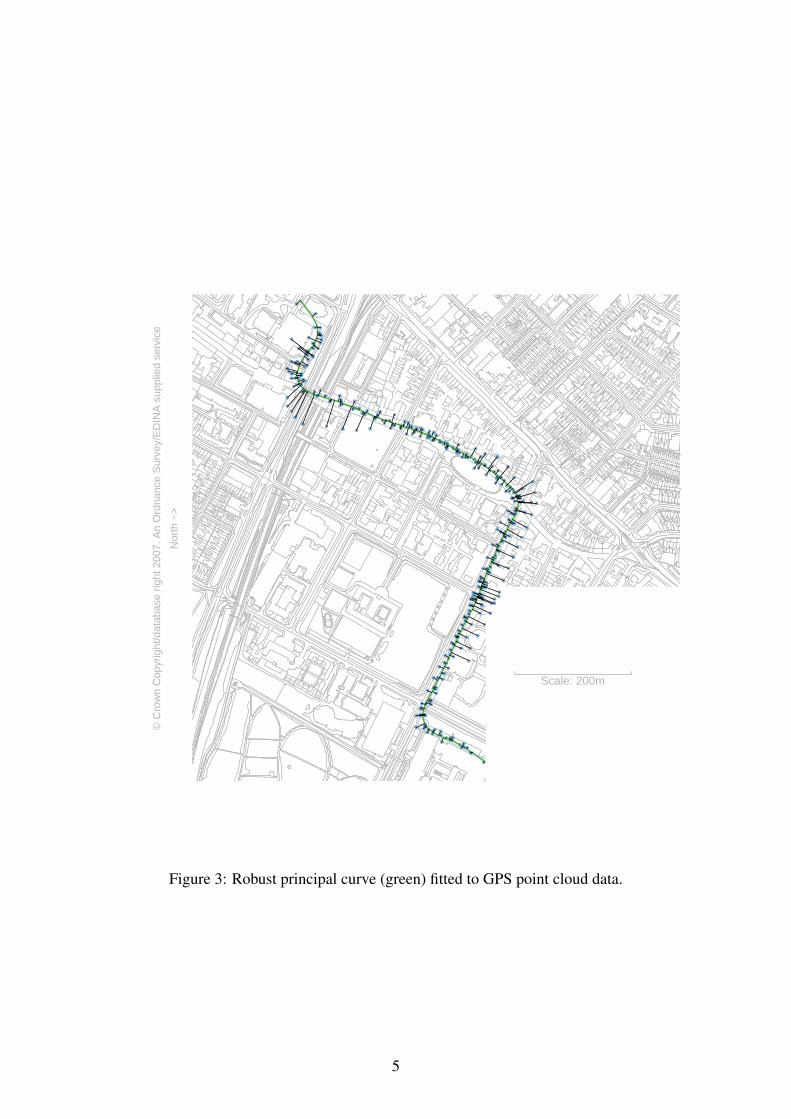
Figure 3: Robust principal curve (green) fitted to GPS point cloud data.

5

5. Re-run the principal curve algorithm, but use weights {wi} in the nonparametric regressionstage.

The result of applying this modified algorithm to the point cloud is shown in figure 3. Fromthis, it is clear that the influence of the rogue track has been greatly reduced, and the estimatedpath now correctly follows the footbridge over the railway and main road.

3. Assessing the Quality of Principal CurvesAs stated earlier, two ways of assessing the quality of the estimated curves are proposed - in termsof accuracy and precision. Accuracy — the ability of the curve to reproduce the ‘ground truth’of path location — may be carried out visually using figures 2 and 3. Here, particularly with therobust modification, the results are encouraging.

Precision is essentially a measure of the reliability of the estimated paths, given that the loggedGPS tracks are samples of locations on the actual paths containing some random error. Here, itis proposed to use a bootstrapping approach (Efron 1981; Effron 1982) to estimate confidencebands around the paths. Briefly, this method estimates the sampling distribution of an arbitarystatistic s from a data set {Xi : i = 1...n} by randomly sampling n items from the data set withreplacement a number of times. Effectively we estimate the true distribution of the Xi’s as a masspoint distribution in which each individual value Xi has a probability of 1

nof occurring.

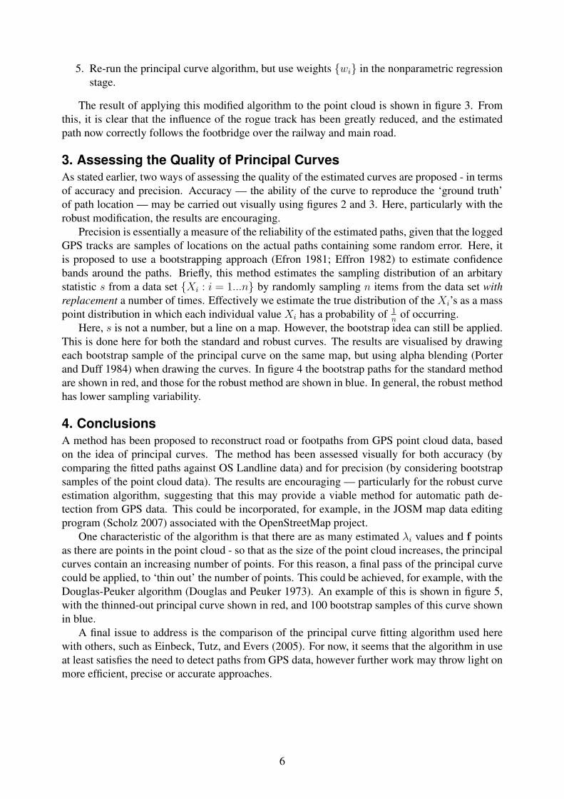
Here, s is not a number, but a line on a map. However, the bootstrap idea can still be applied.This is done here for both the standard and robust curves. The results are visualised by drawingeach bootstrap sample of the principal curve on the same map, but using alpha blending (Porterand Duff 1984) when drawing the curves. In figure 4 the bootstrap paths for the standard methodare shown in red, and those for the robust method are shown in blue. In general, the robust methodhas lower sampling variability.

4. ConclusionsA method has been proposed to reconstruct road or footpaths from GPS point cloud data, basedon the idea of principal curves. The method has been assessed visually for both accuracy (bycomparing the fitted paths against OS Landline data) and for precision (by considering bootstrapsamples of the point cloud data). The results are encouraging — particularly for the robust curveestimation algorithm, suggesting that this may provide a viable method for automatic path de-tection from GPS data. This could be incorporated, for example, in the JOSM map data editingprogram (Scholz 2007) associated with the OpenStreetMap project.

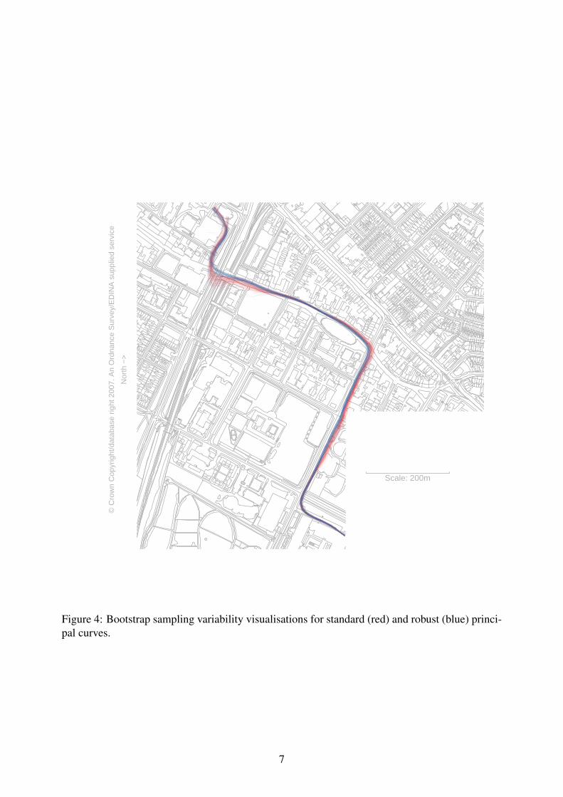
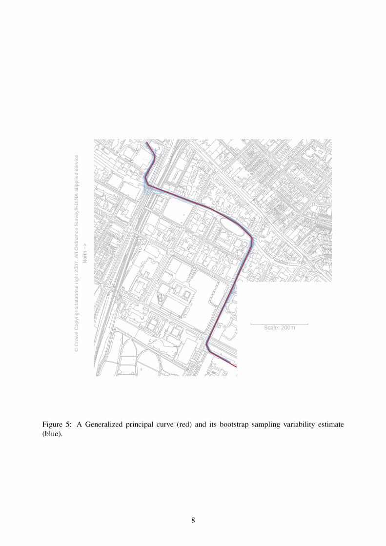
One characteristic of the algorithm is that there are as many estimated λi values and f pointsas there are points in the point cloud - so that as the size of the point cloud increases, the principalcurves contain an increasing number of points. For this reason, a final pass of the principal curvecould be applied, to ‘thin out’ the number of points. This could be achieved, for example, with theDouglas-Peuker algorithm (Douglas and Peuker 1973). An example of this is shown in figure 5,with the thinned-out principal curve shown in red, and 100 bootstrap samples of this curve shownin blue.

A final issue to address is the comparison of the principal curve fitting algorithm used herewith others, such as Einbeck, Tutz, and Evers (2005). For now, it seems that the algorithm in useat least satisfies the need to detect paths from GPS data, however further work may throw light onmore efficient, precise or accurate approaches.

6

© C

row

n C

opyr

ight

/dat

abas

e rig

ht 2

007.

An

Ord

nanc

e S

urve

y/E

DIN

A s

uppl

ied

serv

ice

Nor

th −

>

Scale: 200m

Figure 4: Bootstrap sampling variability visualisations for standard (red) and robust (blue) princi-pal curves.

7

© C

row

n C

opyr

ight

/dat

abas

e rig

ht 2

007.

An

Ord

nanc

e S

urve

y/E

DIN

A s

uppl

ied

serv

ice

Nor

th −

>

Scale: 200m

Figure 5: A Generalized principal curve (red) and its bootstrap sampling variability estimate(blue).

8

5. ReferencesCleveland, W. S, 1979, Robust locally weighted regression and smoothing scatterplots. Journal of

the American Statistical Association 74, 829–836.

Douglas, D and Peuker, T, 1973, Algorithms for the reduction of the number of points required torepresent a digitised line or its caricature. The Canadian Cartographer 10, 112–122.

Effron, B, 1982, The Jacknife, the Bootstrap and Other Resampling Plans. Philadelphia, Pennsyl-vania: Society for Industrial and Applied Mathematics.

Efron, B, 1981, Nonparametric estimates of standard error: the jackknife, the bootstrap and othermethods. Biometrika 68, 589–599.

Einbeck, J, Tutz, G, and Evers, L, 2005, Local principal curves. Statistics and Computing 15,301–313.

Green, P and Silverman, B, 1994, Nonparametric Regression and Generalized Linear Models: ARoughness Penalty Approach. London: Chapman and Hall.

Hastie, T. J and Stuetzle, W, 1989, Principal curves. Journal of the American Statistical Associa-tion 84(406), 502–516.

Porter, T and Duff, T, 1984, Compositing digital images. Computer Graphics 18(3), 253–259.

Scholz, I, 2007, JOSM — OpenStreetMap. Web Site. http://josm.eigenheimstrasse.de/(Viewed April 3, 2007).

The OpenStreetMap Foundation, 2007, OpenStreetMap. Web Site. http://www.

openstreetmap.org (Viewed April 3, 2007).

9