Embed Size (px)
Citation preview

Path dependence in hierarchical organizations:
The influence of environmental dynamics
Arne Petermann
Institute for Quality and Management, BAGSS
Konrad-Zuse-Str 3a, 66115 Saarbrücken, Germany
E-mail: [email protected]
KEYWORDS
agent based modelling, social simulation, path
dependence, path breaking, organizational studies,
business strategy, technology strategy
ABSTRACT
The following paper will describe how path dependent
hierarchical organizations are affected by a changing
environment. The results of current research in this field
(Petermann et al. 2012) analyzed path dependency of
norms and institutions in different kinds of hierarchical
organizations and the impact of leadership within this
process. The results were produced for stable
environments only. Agent based simulation was applied
as research method. In order to examine how this
process evolves when the organizational environment is
changing, the existing model will be enhanced. The
objective is to simulate the impact of external influences
to the emergence of norms within an organization.
INTRODUCTION
Nowadays most organizations have to deal with a
changing environment. From the organizational point of
view a changing environment can be seen as
disturbances from outside, that forces the organization
to adapt. If an organization fails to do so, it may fall
back or even be eliminated from the competition. This
comes with a high risk, especially when new
technologies flood the market and companies have to
react. Examples may be found by taking a closer look at
companies like Loewe or Nokia. Loewe missed the
technological change on the TV market from the CRT
displays to the new LCD-based flat screen technologies.
In fact, Loewe still builds CRT displays. The result is an
imbalance of supply and demand, because most
customers are not interested in those TV’s any more.
Thus Loewe appears ignorant of market realities. The
high technical level of their obsolete skills is disguising
the internal view of the environment, in this case:
innovations on the TV market. In the end the investor
Stargate Capital bought Loewe and made some serious
changes. But their previous ignorance almost led them
into bankruptcy.
Nokia on the other hand was one of the pioneer
companies on the mobile phone market, but they did not
Alexander Simon
Berlin University of Professional Studies
Katharinenstraße 17-18, 10711 Berlin, Germany
E-mail: [email protected]
react adequately to new mobile trends. Just like Loewe,
Nokia suffered immensely when other suppliers like
Apple and Samsung captured the market applying the
latest technologies. By now the mobile phone division
of Nokia has been bought by Microsoft. The questions
that arise are: why do companies sometimes need to get
hit so hard from external influences until they see that
they have to change? How fierce do these influences
need to be?
In the following research the model M1, (Petermann et
al. 2012) which for reasons of simplicity was built on
the assumption of a stable environment will be extended
with a new variable one or the other will include
environmental change into the model.
LITERATURE REVIEW AND RESEARCH
QUESTION
The theoretical concept for the behavioral analysis
described above is called “theory of path dependence”.
The concept of that theory was first described by David
(1985). He dug into the history of the “QWERTY”-
keyboards from their first steps in the 19th century until
1985. This alignment of characters has been dominant
till today for nearly 100 years. In the early 1930s the
alternative “DVORAK” keyboard layout was
developed. In that time this new technology was clearly
a superior solution than the incumbent. These
keyboards, however, were not able to become a serious
competitor to “QWERTY”- keyboards. David examined
in detail the self-reinforcing mechanisms that led to the
domination of the established keyboards by the inferior
QWERTY solution.
Based on David's findings, Arthur (1989) used a polya
urn model to analyze the self reinforcing mechanisms
discovered by David in a more formal way. In his model
two technologies (A and B) are entering the market at
the same time and compete for the adoption by
customers called agents. At the beginning both
technologies have the same chances to get adopted. For
the first time in the history of the path dependence
debate, Arthur coined the definition of the historical
small events increasing returns and contingency. These
events are responsible for the start of the path process
and lead to a lock-in of the technologies A or B. Figure
1(Arthur 1989: 120) illustrates this behavior. When B is
locked in, A is completely eliminated from the market.
Proceedings 30th European Conference on Modelling and Simulation ©ECMS Thorsten Claus, Frank Herrmann, Michael Manitz, Oliver Rose (Editors) ISBN: 978-0-9932440-2-5 / ISBN: 978-0-9932440-3-2 (CD)

Figure 1: Increasing returns adoption: a random walk
with absorbing barriers
David and Arthur stress that a technology can become
dominant even when it is inferior in terms of its long
term value to the system.
Transform path dependence to an organizational
context
To transfer the theory of path dependence to an
organizational context, a different view of Arthur’s
description is needed. In organizations and social
systems history always matters, and due to the ongoing
variations in behavior, the lock-in on markets has
peculiar characteristics. There is less adoption behavior;
hence development phases deviate from purely
technological path dependence. To capture
organizational path dependence, Sydow developed a
model which describes this advanced concept of path
dependence. In this model the path is split into three
different phases. Figure 2 (Sydow et al., 2009: 692)
shows the concept of this model.
Figure 2: The Constitution of an Organizational Path
Phase 1: Preformation Phase
In this phase the decisions the participants are able to
make are relatively open. Influences at this point can be
historical events, “history matters”, routines, and the
existing culture of the organization. In the beginning the
participants already have an idea of thinking and
behaving in their daily environments. Koch (2007: 286)
described imprinting circumstances of an organizational
culture in this context. Therefore the decisions that will
be made in the future are already not completely open.
In figure 2 all options are symbolized by the black stars,
but only the stars in the grey zone are available options
for the organization.
Phase 2: Formation Phase
In this phase the path begins to emerge. The step from
phase 1 to phase 2 is called “critical juncture”. An
unknown or virtually unrecognizable event from the
past leads to the organizational path formation (Sydow
et al., 2009: 693). These events are described as “small
events”. The self-reinforcing effects that are triggered
by these small events narrow the path and limit future
choices within the organization.
Phase3: Lock-In Phase
The reinforcing effects have now taken the lead and
reduced the scope of choices drastically. The
organizational path has become locked-in. The lock-in
state may, in an unfortunate case, be an inefficient one
which disables the organization's ability to change and
adopt more efficient solutions to the problems at hand.
As described, Loewe appeared locked-in to such an
unfortunate state. At first the state was very efficient,
but when the market changed Loewe’s technology was
not needed anymore and thus the state lost its efficiency,
causing severe problems for the organization.
RESEARCH QUESTIONS
We are interested in the impact of a changing
environment to organizations that undergo path
depended processes. In historical analysis scholars have
shown many examples of organizations that were able
to adapt in the light of changing environment, while
others are stuck in a lock-in state, unable to change,
even when the necessity to change became obvious
from an outside perspective. Our model aims at
describing hierarchical organizations, that undergo a
path depended development in a changing environment.
Will they be able to adapt or do they stick to the path?
What can we learn about this process applying
simulation methods? How should an organization be
structured, to be able to adapt in the light of dramatic
changes in the environment?
METHOD
In modern social and management sciences the method
of simulation modeling has been accepted since the
early 1990s (Harrison 2007: 1232). When complexity
and non-linearity of social systems make it hard or
impossible to develop mathematical equations,
simulation models are a good choice to describe the
whole system and its development (Gilbert et al 2005:
16). ‘Simulation is particularly useful when the
theoretical focus is longitudinal, nonlinear, or
processual, or when empirical data are challenging to
obtain’ (Davis et al, 2007: 481). On the other hand, it is
important to know that the method of simulation cannot
replace empirical or analytic methods, but it can provide
insights and first assumptions for other social research
methods.

The basic model
The basics of this research is the simulation model M1
Petermann et al. (2012) developed in their simulation
study about the competing powers of self-reinforcing
dynamics and hierarchy in organizations. The theory of
that model is the simulation of a norm A and a norm B
in an organizational hierarchy structure and to answer
the question which norm will be adopted by most of its
members. Every member of the organization is
represented as an agent. These agents are able to decide
whether to adopt norm A or norm B.
Agents decision algorithm to adopt A or B
To implement this technically, the agents need to be
forced to adopt a norm. Therefore the force-to-act
variable FTA is defined (Petermann et al. 2012: 726).
(1)
Vj describes the connection of individual and
organizational goals according to Vrooms (1964)
expectancy theory. Ej ϵ [0,1] represents the subjective
probability of each agent’s decision. This variable
represents the “small events” of the organizational path
dependence theory. To implement this in the algorithm,
the strictly monotonously increasing function
(2)
is used in the simulation to determine V according to
equation (1) with M ϵ {A, B}, m = 1 for fA,c(x) and m=
-1 for fB,c(x). The variable c represents the reinforcing
effects and is generated by the actual spread ϵ [-1, 1]
which is a variable that characterizes the state of the
system, which is either dominated by agents who all
choose A (spread =-1) or agents who all choose B
(spread=1) or at some state between these extreme cases
(spread between -1 and 1). The factor i(y) sets the value
of li in the correction path direction. This could be 1 or
-1. At the beginning of the simulation the spread is 0
(meaning there are equally large groups of agents
choosing A and B in the beginning of the simulation).
The lock-in state is nearly 1 for A or nearly -1 for B
after a defined amount of time (measured in ticks). The
misfit costs are described by x. The leadership impact
variable li, which makes the simulation of a hierarchy
organizational structure possible, is affecting every
agent according to what norm his supervisor prefers.
Under these conditions the agents choose an adoption
for A, when
(3)
and otherwise B if FTAB > FTAA.
Simulation of an external impact
Enhancing this model further, we now implement an
external impact into the FTA function to see whether or
not this will have an effect of breaking the
organizational path. Therefore, equation (2) needs to be
extended with an additional value.
(4)
The variable ei represents the external impact from the
changing environment. The factor s(z) is only used to
set the correct direction, which depends on the actual
path. The value generation of that variable, needs to be
clarified in the next step. While all other variables in the
equation are generated by the simulated organization
itself, ei is triggered from an external source. When
there is no external impact, ei is equal to 1 and behaves
neutrally. The question of how the model reacts after the
lock-in, has occurred is highly interesting. Are there any
options to “reset” the norm distribution of the
organization? The goal here is to find out about the
behavior of the organization regarding the external
impact. Is its intensity, its continuity, or a mix of both
able to break the path? Every agent in the system is
subject to the same external impacts. We assume that
environmental influences have the same strength
throughout the organization.
SIMULATION
To simulate the described external impact, we need to
specify in what way and when the variable ei should
change. The first condition, we need to break the path
and the path must be locked-in. That means that a
dominant norm exists in the simulation model. The
lock-in state in model M1 is defined by Petermann et al.
(2012: 195) as minimum 500 of ticks with a spread >
0.9 if B is dominant (spread < -0.9 if A is dominant).
Furthermore, a definition for breaking a path is also
needed. The model M1 defines no values for that, so we
assume a path is broken when spread < 0.5, when B was
the current norm in the company and a spread > -0.5
when A was the current norm. This means that less than
75% of all company members adopted a norm. The last
variable is the leadership impact. This is set to 1, to
have an impact from that side. The defined values for
lock-in and leadership impact are assumption and not
empirical researched values.

The variation of the external impact is possible in two
ways. Either the intensity can be variated or the amount
of time (number of ticks) the impact is present in the
system. To get usable data from the simulation model,
only datasets with a lock-in at B before the external
impact is triggered are used for analysis purposes.
Otherwise it is not possible to see a behavior for one
norm. A simulation for each parameter-set will run 100
times according to the Monte-Carlo method (Law et al.
1991:113).
Run of the 1. Simulation
The change of the external impacts must be further
clarified to run the first approach. During the
enhancement of the model the following parameters
seemed to be valid for a first run. After the first
simulation an optimization of the parameters is needed.
Maybe a closer look at several parameter areas is
interesting.
intensity (int)
con
tin
uit
y (
tick
s)
1 3 5 7 10
10 10/1 10/3 10/5 10/7 10/10
40 40/1 40/3 40/5 40/7 40/10
70 70/1 70/3 70/5 70/7 70/10
100 100/1 100/3 100/5 100/7 100/10
130 130/1 130/3 130/5 130/7 130/10
Figure 3: 1. Simulation parameter Setup
The lock-in behavior with leadership impact of 1 and 2
is at 6000 ticks (Petermann et al. 2012:195). This
means, that each simulation must run at least 6000 ticks,
before the external impact can be triggered. A complete
run will last 8500 ticks, and then the system has enough
time to reconfigure itself after the external impact. It is
not possible to define a number of ticks after the impact,
when the system has locked-in again. This basic setup is
used for all simulations in this paper; otherwise it is not
possible to compare the results properly.
Results of the 1st Simulation
The result of this run is a huge amount of data, which
needs to be analyzed. The first intensity parameters
from 1 to 3 will not be visualized in this paper, because
the maximum possible spread change is from 1 to 0,992
at a random point of time, so with a parameter
combination of 130 for continuity and 3 for intensity no
connection to the external impact can be identified. The
effects that occur at the intensity of 10 are also not
visualized they are similar to the graphics that depict the
intensity of 7.
Results for Intensity of 1 and 3
No valid differences could be detected, that change the
system normal behavior. It is not possible, to force a
path break with all combinations containing the
parameter 1 for intensity.
The most interesting effect occurs at the parameter
intensity between 5 and 7.
Results for Intensity of 5
Figure 4: Left: Histograpchical view: probability
density, 150 ticks summarized. X axis: spread, Y axis:
probability from 0-1, z-Axis: time in ticks, starts
counting at 5800 ticks. Right: exemplary first 10 runs. X
Axis: ticks, Y-Axis: spread.
At this parameter setup the system started to react. With
the combination of continuity of 10 until continuity of
70 no valuable reactions are noticeable. However, at a
continuity of 100 the system starts to change. The
spread is forced to the path breaking direction. Of
course, it is only a spread of 0.992, but the events occur
exactly at the starting point of the external impact.
With this first result it is maybe useful, to increase the
continuity over 130 with an intensity of 5 to generate a
path break.

Results for Intensity of 7
F
Figure 5: Left: Histograpchical view: probability
density, 150 ticks summarized. X axis: spread, Y axis:
probability from 0-1, z-Axis: time in ticks, starts
counting at 5800 ticks. Right: exemplary first 10 runs. X
Axis: ticks, Y-Axis: spread.
An intensity of 7 forces the system to break the path for
the first time even with low continuities. With a
continuity of 10 a significant system behavior is
detected, but there is still no path break. This happens
for the first time with a continuity of 40 (spread < 0.4).
Higher continuities with values of 70, 100 and 130
forced the system to establish new norms.
Results for Intensity of 10
The intensity of 10 behaves nearly like the intensity of
7. With higher amount of continuity path breaks and
new path formations are results of the simulation.
Summary of the 1st Simulation
The first simulation run gave first insights to the system
behavior of the described model M1. In the following
three figures all parameter combinations described in
figure 3 are being compared.
The effect at the path is listed in figure 6. As described
above, the interesting area is between the intensities of 5
and 7. The probability of a path breaking behavior
increases rapidly at this interval. This parameter field
will be investigated more closely.
intensity (int)
con
tin
uit
y (
tick
s)
1 3 5 7 10
10 0% 0% 0% 0% 0%
40 0% 0% 0% 99% 100%
70 0% 0% 0% 100% 100%
100 0% 0% 0% 100% 100%
130 0% 0% 0% 100% 100%
Figure 6: Pathbreaking probability
Figure 7 describes the probability of new path
directions. With a continuity of 70 at an intensity of 7
the probability is 3% higher compared to an intensity of
10. There is, however, a small probability at 100
simulation runs that the result differs from one’s
expectations. That the system behaves unexpectedly at
this point could also be an assumption. A deeper
analysis about this could be an interesting question for
upcoming research, but it will not find place in this
paper.
intensity (int)
con
tin
uit
y (
tick
s)
1 3 5 7 10
10 0% 0% 0% 0% 0%
40 0% 0% 0% 0% 0%
70 0% 0% 0% 35% 32%
100 0% 0% 0% 100% 100%
130 0% 0% 0% 100% 100%
Figure 7: new path direction probability
Finally the average spread over all combinations is
shown in figure 8. The average was calculated at the last
tick of the impact. As expected, the spread changes in
the intensity fields of 1 and 3 are out of scope. It’s
interesting to see that with an intensity of 5 differs with
3%, but that is not according to its continuity.
intensity (int)
con
tin
uit
y (
tick
s)
1 3 5 7 10
10 1,00 1,00 1,00 0,84 0,82
40 1,00 1,00 1,00 0,40 0,37
70 1,00 1,00 0,98 0,05 0,02
100 1,00 1,00 0,97 -0,23 -0,25
130 1,00 1,00 1,00 -0,43 -0,45
Figure 8: Average spread, calculated at the last external
impact tick
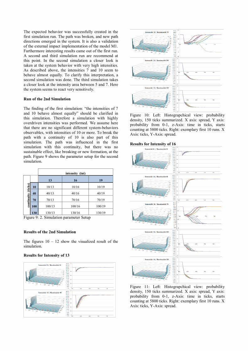
The expected behavior was successfully created in the
first simulation run. The path was broken, and new path
directions emerged in the system. It is also a validation
of the external impact implementation of the model M1.
Furthermore interesting results came out of the first run.
A second and third simulation run are recommend at
this point. In the second simulation a closer look is
taken at the system behavior with very high intensities.
As described above, the intensities 7 and 10 seem to
behave almost equally. To clarify this interpretation, a
second simulation was done. The third simulation takes
a closer look at the intensity area between 5 and 7. Here
the system seems to react very sensitively.
Run of the 2nd Simulation
The finding of the first simulation: “the intensities of 7
and 10 behave almost equally” should be clarified in
this simulation. Therefore a simulation with highly
overdriven intensities was performed. We assume here
that there are no significant different system-behaviors
observables, with intensities of 10 or more. To break the
path with a continuity of 10 is also part of this
simulation. The path was influenced in the first
simulation with this continuity, but there was no
sustainable effect, like breaking or new formation, at the
path. Figure 9 shows the parameter setup for the second
simulation.
intensity (int)
con
tin
uit
y (
tick
s)
13 16 19
10 10/13 10/16 10/19
40 40/13 40/16 40/19
70 70/13 70/16 70/19
100 100/13 100/16 100/19
130 130/13 130/16 130/19
Figure 9: 2. Simulation parameter Setup
Results of the 2nd Simulation
The figures 10 – 12 show the visualized result of the
simulation.
Results for Intensity of 13
Figure 10: Left: Histograpchical view: probability
density, 150 ticks summarized. X axis: spread, Y axis:
probability from 0-1, z-Axis: time in ticks, starts
counting at 5800 ticks. Right: exemplary first 10 runs. X
Axis: ticks, Y-Axis: spread.
Results for Intensity of 16
Figure 11: Left: Histograpchical view: probability
density, 150 ticks summarized. X axis: spread, Y axis:
probability from 0-1, z-Axis: time in ticks, starts
counting at 5800 ticks. Right: exemplary first 10 runs. X
Axis: ticks, Y-Axis: spread.
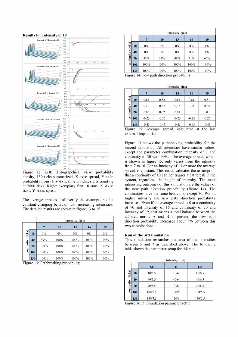
Results for Intensity of 19
Figure 12: Left: Histograpchical view: probability
density, 150 ticks summarized. X axis: spread, Y axis:
probability from -1, z-Axis: time in ticks, starts counting
at 5800 ticks. Right: exemplary first 10 runs. X Axis:
ticks, Y-Axis: spread.
The average spreads shall verify the assumption of a
constant changing behavior with increasing intensities.
The detailed results are shown in figure 13 to 15.
intensity (int)
con
tin
uit
y (
tick
s)
7 10 13 16 19
10 0% 0% 0% 0% 0%
40 99% 100% 100% 100% 100%
70 100% 100% 100% 100% 100%
100 100% 100% 100% 100% 100%
130 100% 100% 100% 100% 100%
Figure 13: Pathbreaking probability
intensity (int)
con
tin
uit
y (
tick
s)
7 10 13 16 19
10 0% 0% 0% 0% 0%
40 0% 0% 0% 0% 0%
70 35% 32% 49% 51% 60%
100 100% 100% 100% 100% 100%
130 100% 100% 100% 100% 100%
Figure 14: new path direction probability
intensity (int)
con
tin
uit
y (
tick
s)
7 10 13 16 19
10 0,84 0,82 0,81 0,81 0,81
40 0,40 0,37 0,35 0,35 0,35
70 0,05 0,02 0,01 0 0
100 -0,23 -0,25 -0,25 -0,25 -0,26
130 -0,43 -0,45 -0,45 -0,45 -0,45
Figure 15: Average spread, calculated at the last
external impact tick
Figure 13 shows the pathbreaking probability for the
second simulation. All intensities have similar values,
except the parameter combination intensity of 7 and
continuity of 30 with 99%. The average spread, which
is shown in figure 15, only varies from the intensity
from 7 to 10. For an intensity of 13 or more the average
spread is constant. This result validates the assumption
that a continuity of 10 can not trigger a pathbreak in the
system, regardless the height of intensity. The most
interesting outcomes of this simulation are the values of
the new path direction probability (figure 14). The
continuities have the same behaviors, except 70. With a
higher intensity the new path direction probability
increases. Even if the average spread is 0 at a continuity
of 70 and intensity of 16 and continuity of 70 and
intensity of 19, that means a total balance between the
adopted norms A and B is present, the new path
direction probability increases about 9% between this
two combinations.
Run of the 3rd simulation
This simulation researches the area of the intensities
between 5 and 7 as described above. The following
table shows the parameter setup for this run.
intensity (int)
con
tin
uit
y (
tick
s)
5,5 6 6,5
10 10/5.5 10/6 10/6.5
40 40/5.5 40/6 40/6.5
70 70/5.5 70/6 70/6.5
100 100/5.5 100/6 100/6.5
130 130/5.5 130/6 130/6.5
Figure 16: 3. Simulation parameter setup
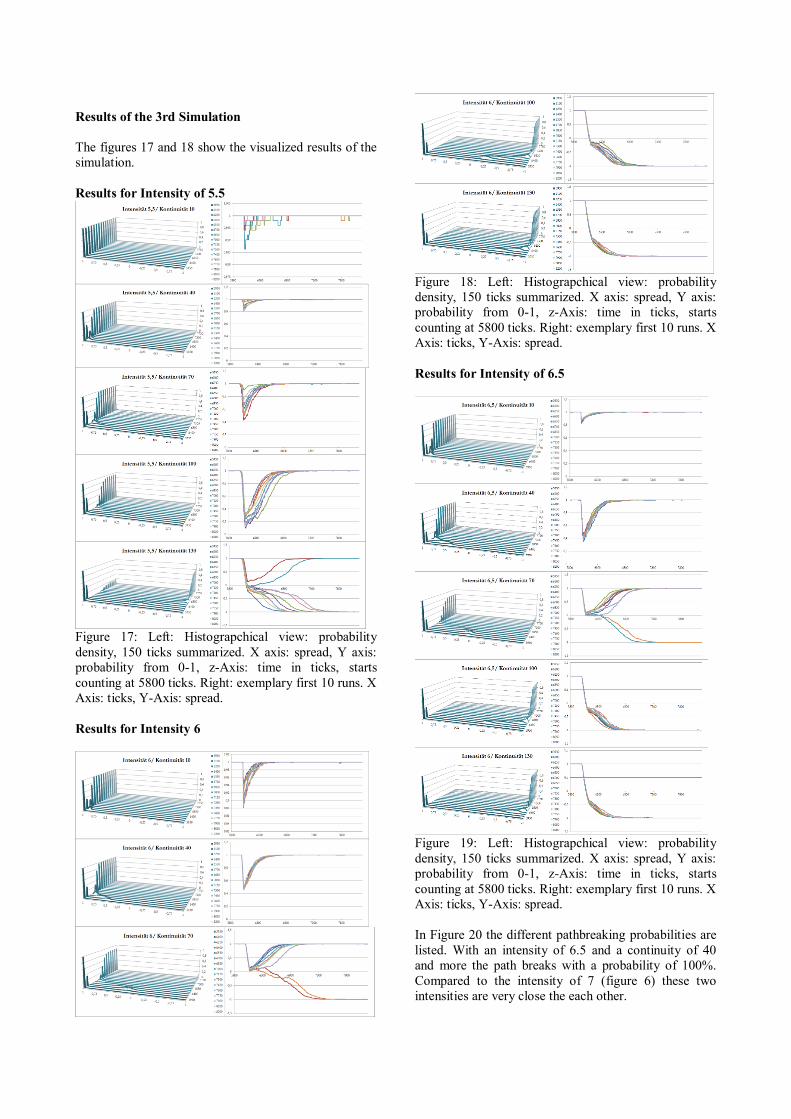
Results of the 3rd Simulation
The figures 17 and 18 show the visualized results of the
simulation.
Results for Intensity of 5.5
Figure 17: Left: Histograpchical view: probability
density, 150 ticks summarized. X axis: spread, Y axis:
probability from 0-1, z-Axis: time in ticks, starts
counting at 5800 ticks. Right: exemplary first 10 runs. X
Axis: ticks, Y-Axis: spread.
Results for Intensity 6
Figure 18: Left: Histograpchical view: probability
density, 150 ticks summarized. X axis: spread, Y axis:
probability from 0-1, z-Axis: time in ticks, starts
counting at 5800 ticks. Right: exemplary first 10 runs. X
Axis: ticks, Y-Axis: spread.
Results for Intensity of 6.5
Figure 19: Left: Histograpchical view: probability
density, 150 ticks summarized. X axis: spread, Y axis:
probability from 0-1, z-Axis: time in ticks, starts
counting at 5800 ticks. Right: exemplary first 10 runs. X
Axis: ticks, Y-Axis: spread.
In Figure 20 the different pathbreaking probabilities are
listed. With an intensity of 6.5 and a continuity of 40
and more the path breaks with a probability of 100%.
Compared to the intensity of 7 (figure 6) these two
intensities are very close the each other.

intensity (int)
con
tin
uit
y (
tick
s)
5.5 6 6.5
10 0% 0% 0%
40 0% 68% 100%
70 22% 100% 100%
100 93% 100% 100%
130 99% 100% 100%
Figure 20: Pathbreaking probability
The new path direction probability increases rapidly
from an intensity of 5.5 to 6 with a continuity of 100
from 6% to 98%, shown in figure 21. The highly
sensitive area can be bounded between the intensities
from 5.5 to 6.
intensity (int)
con
tin
uit
y (
tick
s)
5,5 6 6,5
10 0% 0% 0%
40 0% 0% 0%
70 0% 12% 18%
100 6% 98% 100%
130 81% 100% 100%
Figure 21: new path direction probability
Also the average spread in figure 22 has a very sensitive
reaction in this parameter area. The combination
intensity of 5.5 and continuity of 10 has no valuable
effect on the spread, but the spread changes with an
increasing continuity to the direction of the forced
norm.
intensity (int)
co
nti
nu
ity (
tick
s)
5,5 6 6,5
10 1,00 0,91 0,85
40 0,92 0,48 0,42
70 0,64 0,11 0,07
100 0,25 -0,18 -0,21
130 -0,07 -0,39 -0,41
Figure 22: Average spread, calculated at the last
external impact tick
Conclusion
The aim of this research was to examine the behavior of
external influences of a path dependent hierarchical
organization with the method of computer simulation.
The basis of the simulation was the M1 model from
Petermann (2012) that simulates a path dependent
hierarchical organization. The model was enhanced to
simulate an external impact in form of continuity and
intensity which were combined and incorporated into
the M1 model. For the first simulation a parameter setup
that seemed to be valid during the implementation of the
external impact was used. With the first results multiple
questions arose and two more simulations with adjusted
parameter setups were executed. To get an overview of
the three simulations figure 23 shows an interesting
chart spread versus intensity.
Figure 23: Spread vs intensity. X-axis: intensity. Y-axis:
spread. Legend: Continuities from 10-130
To see a reaction on the system a critical intensity is
needed. An intensity of 3 and less has no effect on the
spread. The system first starts to react at the
combination of intensity 3 and continuity of 100. As
described in the third simulation, with an intensity of 5
the spread changes dramatically, but the intensive
change stops immediately at the intensity of 6 and over.
In this intensity field the external impact must last for a
defined continuity to adopt a new norm in the whole
company. The defined leadership impact of 1 concludes
that with an intensity of 5, which is the minimum value
to change the spread, the external impact needs to be
five times stronger than the leadership impact. To
clarify this, further research might show results.
Figure 24: Probability for a new path direction with a
continuity of 70. X-axis: intensity, y-axis: new path
direction probability. Legend: continuity of 70
Another interesting result of this research is the new
path direction probability. It was not in scope at the
beginning of this research, but we figured out that we
discovered an interesting system behavior at the
continuity of 70 that leads the spread to 0 with

intensities of 13 and more. This probability increases
more and more, the higher the intensity becomes. This
unexpected system behavior should be investigated
further in the future.
The next interesting point is the fact that path breaking
does not necessarily lead to a new path direction. With a
continuity of 40 and an intensity of 6.5 the path
breaking probability is 100%, but the new path direction
probability is 0%. The question that comes up here is:
does it make sense to speak about breaking the path
without actually changing the path? This might indicate
the necessity to adapt the definition of path breaking in
this context.
REFERENCES
Arthur, B. 1989. “Competing technologies, increasing returns
and lock-in by historical events.” The Economic Journal, 99 (March 1989), 116-131.
David, P. 1985. “Clio and the Economics of QWERTY.”
Economic History, Vol. 75, No. 2, 332-337
Davis, P, Eisenhardt, K. and Bingham, C. 2007. “Developing
Theory through Simulation Methods.” Academy of
Management Review,Vol. 32, No 4, 480-499.
Gilbert, N. and Troitzsch, K 2005. “Developing Theory
through Simulation Methods.” 2. ed, Berkshire: Open
University Press
Harrison, J, Lin, Z. and Carroll, G. 2007. “Simulation
Modeling In Organizational And Management Research.”
Academy of Management Review, Vol. 32, No. 4, S. 1229-1245.
Koch, J 2007: Strategie und Handlungsspielraum: Das
Konzept der strategischen Pfade. Zeitschrift Führung + Organisation, 76(5): 283-291
Sydow, J, Schreyögg, G. and Koch, J. 2009. Organizational
path dependence: Opening the black box. Adademy of Management Review, Vol. 34, No. 4, 689-709
Petermann, A., Klaußner, S., Senf, N.: Organizational Path
Dependence: The Prevalence of Positive Feedback Economics in Hierarchical Organizations, in: Troitzsch, K. G., Möhring,
M., Lotzmann, U. (Hrsg.): Proceedings 26th European
Conference on Modeling and Simulation, Koblenz 2012, 721-
730.
Vroom, V.H. 1964. Work and motivation, New York
Prof. Dr. Arne Petermann is Professor of
Management at the Berufsakademie für
Gesundheits- und Sozialwesen Saarland
(BAGSS). He is also Director of the
Institute for Management and Quality at
BAGSS. As a visiting scholar, he was
teaching organization science and scientific simulation
methods in the PhD-program at the School for Business
and Economics at Freie Universität Berlin from 2007 to
2014. He is founder and CEO of Linara GmbH, an
international HR agency specialized in the transnational
European healthcare sector. He is also founder and CEO
of 3P Projects GmbH, a consulting and executive
education company based in Berlin, Germany. His
research focuses on organization science, path-
dependence theory, entrepreneurship, and social
simulation, especially agent-based modeling. His
research results have been presented at the leading
international science conferences in his field, including
the Academy of Management and the American
Marketing Association Educators Conference where,
moreover, his work was recognized with a best paper
award. His work is published in books and peer-
reviewed journals.
Alexander Simon, MBA was born in Rheinfelden,
Germany and studied electrical engineering at the
University of Applied Sciences in St. Augustin,
Germany and Business Administration Berlin
University of Professional Studies. After first
professional experience in the area of software
development with focus on the .NET framework in
telecommunication and biotech industry, he works in
the tax advisory division of Ernst & Young since 2014.
During his MBA program at the Berlin University for
Professional Studies he became acquainted with path-
dependence theory.