Patch Mosaic for Fast Motion Deblurring - ICS | UC Irvine

Patch Mosaic for Fast Motion Deblurring

Hyeoungho Bae,1 Charless C. Fowlkes,2 and Pai H. Chou 1

1 EECS Department, University of California, Irvine2 Computer Science Department, University of California, Irvine

Abstract. This paper proposes using a mosaic image patches composedof the most informative edges found in the original blurry image for thepurpose of estimating a motion blur kernel with minimum computationalcost. To select these patches we develop a new image analysis tool toefficiently locate informative patches we call the informative-edge map.The combination of patch mosaic and informative patch selection enablesa new motion blur kernel estimation algorithm to recover blur kernelsfar more quickly and accurately than existing state-of-the-art methods.We also show that patch mosaic can form a framework for reducing thecomputation time of other motion deblurring algorithms with minimalmodification. Experimental results with various test images show thatour algorithm to be 5-100 times faster than previously published blindmotion deblurring algorithms while achieving equal or better estimationaccuracy.

1 Introduction

Motion blur due to relative motion between the camera and the scene duringcamera exposure plagues consumer photographs, particularly under low-lightconditions. Methods that remove such blur from a single photograph are of greatpractical interest. Thanks to recent advances in image deblurring algorithms, itis now possible to recover unblurred images from blurry sources caused by mo-tion that is not compensated by the optical or mechanical image-stabilizationdevices integrated in modern digital cameras. However, due to the intensivecomputational requirements, the motion-blur deconvolution process of an HD-sized image typically takes several to tens of minutes, thereby precluding theiradaptation in mainstream consumer products. The goal of this research is to de-velop a computationally cheap blind-motion deconvolution algorithm with goodperformance.

1.1 Fast Blind Motion Deblurring and Patch Mosaics

The motion blur can be modeled as a point spread function (or a motion blurkernel) for each point in the image. The relation between the blurry image B,the latent image I, the motion blur kernel k, and noise n can be defined byEquation (1):

B(x, y) = I ⊗ kx,y + n (1)

2 Hyeoungho Bae, Charless C. Fowlkes, and Pai H. Chou

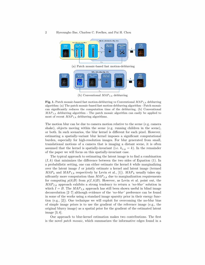
(a) Patch mosaic-based fast motion-deblurring

(b) Conventional MAPI,k deblurring

Fig. 1. Patch mosaic-based fast motion-deblurring vs Conventional MAPI,k deblurringalgorithm: (a) The patch mosaic-based fast motion-deblurring algorithm - Patch mosaiccan significantly reduces the computation time of the deblurring. (b) ConventionalMAPI,k deblurring algorithm - The patch mosaic algorithm can easily be applied tomost of recent MAPI,k deblurring algorithms.

The motion blur can be due to camera motion relative to the scene (e.g. camerashake), objects moving within the scene (e.g. running children in the scene),or both. In such scenarios, the blur kernel is different for each pixel. However,estimating a spatially-variant blur kernel imposes a significant computationalburden, especially for high-resolution images. For blur generated from small,translational motions of a camera that is imaging a distant scene, it is oftenassumed that the kernel is spatially-invariant (i.e. kx,y = k). In the remainderof the paper we will focus on this spatially-invariant case.

The typical approach to estimating the latent image is to find a combination(I, k) that minimizes the difference between the two sides of Equation (1). Ina probabilistic setting, one can either estimate the kernel k while marginalizingover the latent image I or jointly estimate a kernel and latent image (termedMAPk and MAPI,k respectively by Levin et al., [1]). MAPk usually takes sig-nificantly more computation than MAPI,k due to marginalization requirementsfor computing p(k|B) from p(I, k|B). However, as Levin et al. point out, theMAPI,k approach exhibits a strong tendency to return a ‘no-blur’ solution inwhich I = B. The MAPI,k approach has still been shown useful in blind imagedeconvolution [2–7] although evidence of the ‘no-blur’ preference can be foundin some of the works using a standard image sparsity prior in their energy func-tion (e.g., [2]). One technique we will exploit for overcoming the no-blur biasof simple image priors is to use the gradient of the reference image (e.g., theoriginal blurry image) as a spatial prior for the gradient of the estimated latentimage [3, 4].

Our approach to blur-kernel estimation makes two contributions. The firstis the novel patch mosaic, which summarizes the informative edges found in a

Patch Mosaic for Fast Motion Deblurring 3

blurry image. We construct the patch mosaic by tiling informative image patchesto synthesize a new, compact blurry image. Using the patch mosaic, we caneffectively reduce the blur-kernel estimation time. Since only the informativepart of the image is used, there is no need to calculate sophisticated masks foroccluding unwanted parts (saturated or filled with narrow edges) of the imagefor every single iteration such as those found in [4, 6].

To locate patches containing informative edges efficiently, we develop a toolnamed informative-edge map. It can locate edges satisfying several attributes ofinformative edges including contrast, orientation angle, straightness [8], and use-fulness [4]. Through the performance evaluation, we show that the informative-edge map locates the most appropriate area within the blurry image to estimatethe blur kernel and yields the most accurate results while consuming only 4% ofthe computation time of the kernel estimation process.

We integrated these two components into a new, fast motion-deblurring algo-rithm. The computation time of our algorithm is 5 to 40 times faster than thosein the comparison group, while the benchmark estimation accuracy is the bestamong the group, which is shown in Section 3. Our algorithm implemented inMATLAB takes 15 seconds to estimate a 2256×1504-pixel latent color image ona Intel Core i7 processor. Since our framework (shown in Fig. 1) is compatiblewith most of the recent MAPI,k motion-deblurring algorithms, we can apply thepatch mosaic framework as a generic tool for reducing computation time of otherblind motion-deblurring algorithms. To demonstrate the feasibility of this idea,we modified the deblurring algorithm by Krishnan et al. [9]. The results showthat the modified algorithm runs 4.7 times faster than the original algorithmwith similar estimation accuracy.

1.2 Related Work

To our best knowledge, there has been no previous work that uses an imagepatch mosaic for blur-kernel estimation. We briefly discuss two closely relatedlines of work: patch-based image analysis and fast motion deblurring.

Patch-based image analysis: Jia suggested using small fractions of an im-age for blind deconvolution [5]. However, their work needs user intervention forselecting appropriate areas and foreground and background colors for alpha-blending calculation. A larger number of patches increases the complexity ofthe energy function for estimating the blur kernel and latent image. If there islittle distinction between the foreground and background objects, the algorithmyields inaccurate estimation results as shown in [3]. Joshi et al. analyzed theedge profile of an image to predict the latent edge [6]. This is related to thefilter-based sharp edge prediction method as in [2–4], but is limited to blurryedges caused by simple motions orthogonal to the edge. In contrast, our measureseeks patches that individually contain many different orientation angles. In thearea of spatially variant motion-deblurring algorithms, Gupta et al. estimatedthe camera trajectory by patch-based analysis of the scene [10]. However, theyapplied the blind deconvolution algorithm of [3] for the entire image area first.Then, they used RANSAC-based approach to select appropriate results among


initially deblurred image patches to reconstruct the camera motion. We use ourimage-patch locating algorithm to find the most informative image patches be-fore estimating the blur kernel. Our method requires neither user interventionduring the selecting process nor computationally expensive initial deconvolutionstep.

Fast motion deblurring algorithms: Several works address reducing the com-putation time of blind motion-deblurring algorithms [2,4,6,11]. Cho and Lee takethe MAPI,k approach and use discrete Fourier transform to reduce the compu-tation time. However, they still need to use the whole image area to estimatethe blur kernel, which requires their compiled C++ binary 4 to 6 times morecomputation time compared to our interpreted Matlab script. As mentioned ear-lier, their algorithm also seems to prefers ‘no-blur’ results for some cases. Eventhough the accuracy of Xu and Jia’s algorithm is remarkable, the computationtime of their C++ binary code is more than 27 times slower than our Matlabscript due to the sophisticated masking and the larger number of iterations toincrease the accuracy [4]. By using the patch mosaic, we can achieve even betteraccuracy, as quantitative analysis will show in Section 3. Krishnan et al. takea MAPI,k approach but with l1/l2 regularization to predict the latent imagein a coarse-to-fine iteration [11]. However, they still need more than 5 minutesto estimate a color latent image of 558×858 pixels. The authors of [4] has de-veloped a fast deblurring software using GPU. However, our work is targetingmore light-weight platforms like smart phones or portable cameras. So we don’tthink that kind of approach can be regarded as our competitor since it requireshuge computation resources compared to ours. There is also work on speedingup non-blind deconvolution [9, 12] where the kernel is known. Such work couldbe used as a final step in combination with our approach for quickly estimatingthe kernel.

2 Blur-Kernel Estimation Algorithm

The blur-kernel estimation algorithm (Fig. 1) is composed of four parts: (1)Image-patch selection, (2) Patch-mosaic construction, (3) Blur-kernel estimationand (4) Latent image-patch estimation. In image-patch selection, the algorithmfinds a set of patches that cover all possible edge-orientation angles and are likelyto be informative for estimating blur. After selecting the image patches, theselected image patches are combined to construct the patch mosaic for the blur-kernel estimation step. We estimate the kernel from this mosaic using a coarse-to-fine iteration where in each step the estimated blur kernel is deconvolvedwith the individual image patches to estimate the latent image patches. Thesedeblurred patches are then upsampled and used as the image prior for the nextiteration.

2.1 Image-Patch Selection

The main concern of our approach is how to reduce the amount of data to processwithout sacrificing estimation accuracy. As described in several publications,


(a) Located patches (b) IE map

50 100 150 200 250 300 350 400

50

100

150

200

250

300 0

0.1

0.2

0.3

0.4

0.5

0.6

0.7

0.8

0.9

(c) Straightness map

50 100 150 200 250 300 350 400

50

100

150

200

250

300 0

0.1

0.2

0.3

0.4

0.5

0.6

0.7

0.8

0.9

(d) Usability map

Fig. 2. Selected image area: (a) The location of selected image patches . (b) Theinformative edge map from Equation (2). The edges of highest IE value located inthe rectangle box with angle between −9◦ and 9◦. (c) The straightness map (d) Theusability map.

edges found in the original blurry image are particularly useful for estimatingthe blur kernel caused by motion. There are several important characteristicsof edges in motion deblurring; gradient magnitude, orientation angle, width ofthe edges, and straightness of the edges [2–8,13]. Applying masks on top of theblurry image is a common approach to make the estimation algorithm focus onthe most informative areas in the image [4, 6, 8, 10]. However, this does notreduce the actual amount of data to be processed. Moreover, computation ofcomplex masks takes significant additional time [4, 8]. For this reason, someprevious works require user intervention to select the most informative area inthe image [9, 13]. By using the patch mosaic, our approach avoids the need toconstruct a sophisticated mask for the whole image.

Fig. 2 shows an illustrative example of the image-patch selection process.We use the gradient magnitude of a downsampled image to locate the sharpestedges. The blurred trajectory of an edge provides information for estimatingone-dimensional motion that is perpendicular to the edge orientation. To securesufficient information about all possible directions of motion and to recover thefull 2D kernel, it is necessary to analyze edges that span the full range of orien-tations. We start with a pixel-wise measure of informativeness that incorporatesour desired criteria. We specify the informativeness of a pixel by

IE = M ◦ (sR > τs) ◦ (U > τu), (2)

where IE means the validity of information of the edge, M is the gradient mag-nitude of the image, and sR and U are the straightness map from by Cho [8] andusability map by Xu et al. [4], respectively. τs and τu are the threshold valuesfor filtering non-straight edges and less-usable edges, respectively. To ensure thatwe can recover motion in any direction, we also ensure diversity in the angles ofthe edges in selected patches. We define a pixel-wise angle mask that identifiesthose pixels whose gradient falls in given range of angles

angle maski = Qin

[arctan

(5By

5Bx

)], (3)

where Qin means the quantization function to make the ith angle mask among n

groups. For example, in Fig. 2(b), IE is masked to pick out angles between −9◦

and 9◦.


Algorithm 1 Patch Selection

Input: M , sR, U , angle mask , maxpatchP ← {}A← set of angles to coverwhile (|P | < max patch)&(|A| > 0) do

IE ←M ◦(∑

i∈A angle maski)◦ (sR > τs) ◦ (U > τu)

x← largest element of IEP ← P ∪ {x}A← A− angle(x)M ←M − near(x)

end whileOutput: patch locations P

angle(x) is the range of angles in which x fallsnear(x) is the elements near the coordinate of x

The pseudo code for selecting image patches is shown in Algorithm 1. Duringthe iteration, the IE map is masked using the orientation angles not yet cov-ered, so that orientation angles already contained in the set of selected imagepatches will not be included in the sum of the angle mask in Equation (2). Sincethe usefulness map and the straightness map used in the equation have a highcomputational cost, we downsample the original image. Unlike [4], our algorithmdoes not need to use mask for noisy edges or saturated area since we use rel-atively small areas filled with strong edges of homogeneous orientation anglescompared to other algorithms using the entire image area. In our performanceevaluation, we choose the size of image patch to be 5 times that of the initialkernel size, which is 3× 3 pixels.

2.2 Patch Mosaic Construction

The tricky part of using multiple image patches is estimating a single blur kernelsatisfying all the patches. The authors of [5] introduced multiple alpha-blendingvariables into the energy function, while [8] merge using the inverse Radon trans-form. However, these approaches are computationally expensive, and we havefound that the latter introduces noise into the final result. Instead, we merge thepatches to make a single patch mosaic that contains sufficient information toestimate the blur kernel with minimum computation cost (see Fig. 3(a)). Sincewe use a single image, we do not need to introduce multiple variables into theenergy function. Even though our patch mosaic is composed of patches contain-ing single orientation angles, we do not suffer from noise caused by the 1-D blurintegration profile analysis and inverse Radon transform for merging the kernelestimation of individual patches. Instead, the merging happens implicitly in thede-convolution by the constraint of the kernel being spatially invariant.

Simply tiling the image patches from different areas of an image introducesa discontinuity of gradient between adjacent patches and introduces errors inthe recovered kernel (shown in Fig. 3(a)). To solve this problem, we mask out


(a) Patch mosaic (b) With mask

5 10 15 20 25 30 35

5

10

15

20

25

30

35

(c) With mask

5 10 15 20 25 30 35

5

10

15

20

25

30

35

(d) Without mask

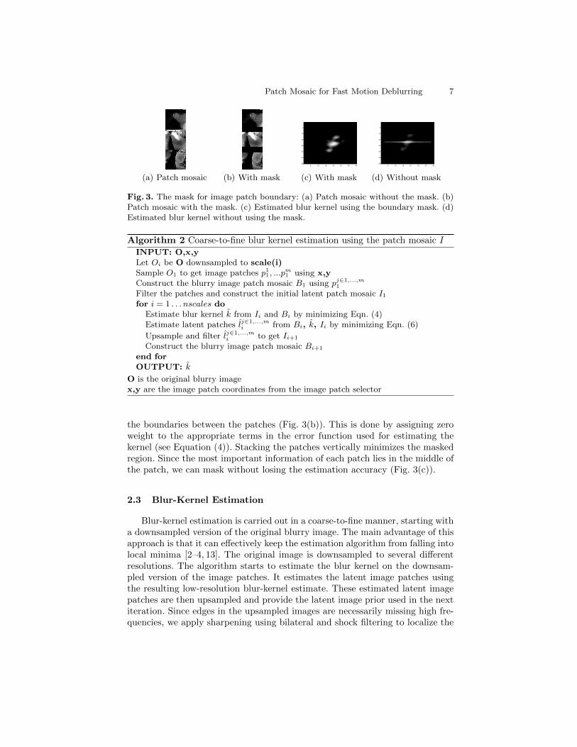
Fig. 3. The mask for image patch boundary: (a) Patch mosaic without the mask. (b)Patch mosaic with the mask. (c) Estimated blur kernel using the boundary mask. (d)Estimated blur kernel without using the mask.

Algorithm 2 Coarse-to-fine blur kernel estimation using the patch mosaic I

INPUT: O,x,yLet Oi be O downsampled to scale(i)Sample O1 to get image patches p11, ...p

m1 using x,y

Construct the blurry image patch mosaic B1 using pj∈1,...,m1

Filter the patches and construct the initial latent patch mosaic I1for i = 1 . . . nscales do

Estimate blur kernel k from Ii and Bi by minimizing Eqn. (4)Estimate latent patches lj∈1,...,mi from Bi, k, Ii by minimizing Eqn. (6)

Upsample and filter lj∈1,...,mi to get Ii+1

Construct the blurry image patch mosaic Bi+1

end forOUTPUT: k

O is the original blurry imagex,y are the image patch coordinates from the image patch selector

the boundaries between the patches (Fig. 3(b)). This is done by assigning zeroweight to the appropriate terms in the error function used for estimating thekernel (see Equation (4)). Stacking the patches vertically minimizes the maskedregion. Since the most important information of each patch lies in the middle ofthe patch, we can mask without losing the estimation accuracy (Fig. 3(c)).

2.3 Blur-Kernel Estimation

Blur-kernel estimation is carried out in a coarse-to-fine manner, starting witha downsampled version of the original blurry image. The main advantage of thisapproach is that it can effectively keep the estimation algorithm from falling intolocal minima [2–4, 13]. The original image is downsampled to several differentresolutions. The algorithm starts to estimate the blur kernel on the downsam-pled version of the image patches. It estimates the latent image patches usingthe resulting low-resolution blur-kernel estimate. These estimated latent imagepatches are then upsampled and provide the latent image prior used in the nextiteration. Since edges in the upsampled images are necessarily missing high fre-quencies, we apply sharpening using bilateral and shock filtering to localize the


(a) Patch mosaic during the kernel estimation

(b) Original image (c) Estimated latent image

Fig. 4. Patch mosaic based blur kernel estimation: (a) Patch mosaic during the kernelestimation - Bi, Ii, and ki represent the blurry patch mosaic, latent patch mosaic andthe estimated blur kernel, respectively. (b) The original blurry image (c) The estimatedlatent image

edges. As mentioned previously, image-patch selection is also carried out on thelow-resolution version of the blurry image.

Given an estimate of the latent image I, the energy function used for esti-mating the blur kernel is given by:

k = arg mink

[‖5I ⊗ k −5B‖2M + γ‖k‖2

], (4)

where I is the latent estimation for the patch mosaic, k is the blur kernel, and B isthe original patch mosaic. The squared error is only computed on those unmaskedpixels specified by the mask M . We set the coefficient (γ) value as 0.001. Duringthe blur kernel estimation process, we used energy function having L2 norm form,which is computationally cheap. According to Plancherel’s theorem, the Fouriertransform is an isometry so we can analyze the squared error in the frequencydomain. This means that minimizing Equation (4) is an identical process tominimizing the frequency domain version of it [14].

k = F−1

(F(5Ix,M ) ◦ F(5Bx,M ) + F(5Iy,M ) ◦ F(5By,M )

F(5Ix,M ) ◦ F(5Ix,M ) + F(5Iy,M ) ◦ F(5Iy,M ) + γ

), (5)

where I means the predicted latent image from the blurry image. To preventthe boundary artifact, the mask mentioned in Section 2.2 is applied after takingthe gradient. We use the predicted latent image from the previous iteration as


0

2 0 0

4 0 0

6 0 0

8 0 0

1 0 0 0

1 2 0 0

2 0 9 . 0 4 s e c

9 8 0 . 9 4 s e c

K r i s h n a n ( m o d . )

K r i s h n a n ( o r g . )tim

e (se

c)

F e r g u s e t a l .

C h o e t a l .

X u e t a l .

O u r s1 4 . 9 5 s e c

4 0 5 . 7 5 s e c

7 2 . 1 1 s e c

1 2 6 0 . 9 0 s e c

(a) Computation time

0 . 4 1 %4 %4 . 8 2 %

1 0 . 8 8 %

1 4 . 6 9 %2 4 . 7 6 %

4 0 . 4 5 % l a t e n t i m a g e p r e d i c t i o n l a t e n t i m a g e e s t i m a t i o n p a t c h m o s a i c c o n s t r u c t i o n k e r n e l t h r e s h o l d k e r n e l e s t i m a t i o n i m a g e p a t c h l o c a t i n g e t c

C o m p u t i n g t i m e a n a l y s i s o f b l u r k e r n e l e s t i m a t i o n l o o p

(b) Blur kernel estimation loop

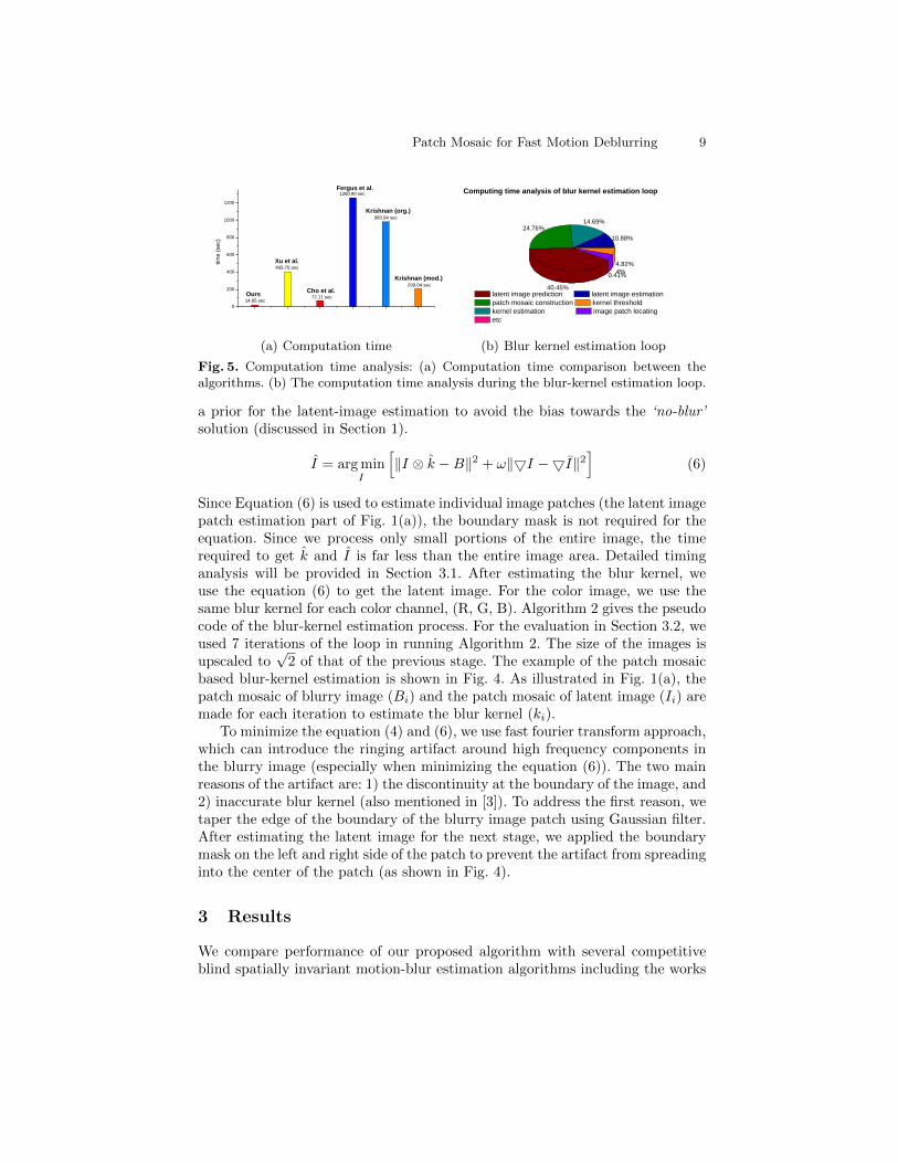
Fig. 5. Computation time analysis: (a) Computation time comparison between thealgorithms. (b) The computation time analysis during the blur-kernel estimation loop.

a prior for the latent-image estimation to avoid the bias towards the ‘no-blur’solution (discussed in Section 1).

I = arg minI

[‖I ⊗ k −B‖2 + ω‖5I −5I‖2

](6)

Since Equation (6) is used to estimate individual image patches (the latent imagepatch estimation part of Fig. 1(a)), the boundary mask is not required for theequation. Since we process only small portions of the entire image, the timerequired to get k and I is far less than the entire image area. Detailed timinganalysis will be provided in Section 3.1. After estimating the blur kernel, weuse the equation (6) to get the latent image. For the color image, we use thesame blur kernel for each color channel, (R, G, B). Algorithm 2 gives the pseudocode of the blur-kernel estimation process. For the evaluation in Section 3.2, weused 7 iterations of the loop in running Algorithm 2. The size of the images isupscaled to

√2 of that of the previous stage. The example of the patch mosaic

based blur-kernel estimation is shown in Fig. 4. As illustrated in Fig. 1(a), thepatch mosaic of blurry image (Bi) and the patch mosaic of latent image (Ii) aremade for each iteration to estimate the blur kernel (ki).

To minimize the equation (4) and (6), we use fast fourier transform approach,which can introduce the ringing artifact around high frequency components inthe blurry image (especially when minimizing the equation (6)). The two mainreasons of the artifact are: 1) the discontinuity at the boundary of the image, and2) inaccurate blur kernel (also mentioned in [3]). To address the first reason, wetaper the edge of the boundary of the blurry image patch using Gaussian filter.After estimating the latent image for the next stage, we applied the boundarymask on the left and right side of the patch to prevent the artifact from spreadinginto the center of the patch (as shown in Fig. 4).

3 Results

We compare performance of our proposed algorithm with several competitiveblind spatially invariant motion-blur estimation algorithms including the works


(a) Test images

1 . 5 2 . 0 2 . 5 3 . 0 3 . 5 4 . 00

2 0

4 0

6 0

8 0

1 0 0

perce

ntage

E r r o r r a t i o

O u r s X u e t a l C h o e t a l F e r g u s e t a l K r i s h n a n ( o r g . ) K r i s h n a n ( m o d . )

(b) Error ratio comparison

Fig. 6. Performance comparison: (a) Test images: From the top-left corner in clock-wise order, “Downtown”, “Fisherman”, “Sealion”, and “Storybook”, (b) Error ratiocomparison.

of Fergus et al., Krishnan et al., Cho and Lee, and Xu and Jia [2, 4, 11, 13].The evaluation is based on three criteria: (1) computation time, (2) quantita-tive analysis on the estimation accuracy using the test images with known blurkernels, and (3) tests for real-world images 1.

3.1 Computation Time

We compared the computation time with the competitive algorithms using thetest images of 2256×1504 resolution used in Section 3.2 (Fig. 5). Our and Fer-gus’s algorithms are written in Matlab script. Xu and Jia’s and Cho and Lee’salgorithms are C/C++ compiled binaries. The experimental platform was a lap-top with an Intel Core-i7 processor with 6 GB RAM. In Fig. 5(a), the averagecomputation time of our algorithm is 14.95 seconds, which is 4.8 times fasterthan the compiled binary version of the fastest algorithm (Cho and Lee’s). Ouralgorithm is 27 times faster than Xu and Jia’s and 84 times faster than Ferguset al.’s. Since our algorithm is not a C/C++ compiled binaries, we expect acompiled version of our algorithm will achieve even faster runtime.

Fig. 5(b) shows the timing breakdown of our algorithm: 44% (6.55 sec) is usedfor the final latent-image estimation for calculating with Equation (6) from [15]and 53% of the time is used for our blur-kernel estimation algorithm. The mosttime-consuming part is the latent-image prediction, which uses bilateral/shockfilters for sharpening the upsampled latent image patches in each iteration. Thesecond largest portion is used for the patch-mosaic construction step. Only 25.5%of the time is used for calculating Equations (4) and (6) during the estimationprocess. It is also worth noting that once the kernel has been estimated, thenon-blind deblurring of the whole image takes a significant proportion of thetime (43.4%, 6.5 sec from 14.95 sec). The patch location and mosaic constructiontake only 14.8% of the total time for the whole deblurring process. If we consider

1 The executable of our algorithm can be downloaded from http://cecs.uci.edu/

~hyeoungho/image_deblur.html


(a) Original image (b) Ours (c) Xu and Jia [4]

(d) Cho and Lee [2] (e) Fergus et al. [13] (f) Krishnan et al. [11]

Fig. 7. Image deblurring results of one blurry “Downtown” image: (a) is the croppedarea from the original blurry image.

the time reduction in the blur-kernel estimation process enabled by the patchmosaic, the portion will be much less than that. We thus achieve more than 400%performance improvement in computation time over competitive algorithms forkernel estimation.

3.2 Estimation Accuracy

For the quantitative analysis of the accuracy of estimated blur kernel, we use theanalysis methodology of Levin et al. [16]. We use the kernels that Levin et al.used in their work 2 and the four images of 2256×1504 pixels shown in Fig. 6(a)to make 32 different blurry images. Fig. 6(b) compares the performance of thefour algorithms including ours.3 SSDE stands for the sum of squared differencesbetween the two images. The error ratio is used to evaluate the accuracy ofestimated blur kernels independently of the error introduced by deconvolution.For this purpose, Richardson-Lucy non-blind image deconvolution algorithm isused for the latent image estimation [17,18].

Generally, our algorithm yields the most accurate blur kernels compared toother competitive algorithms in the group. The blur kernels estimated by ouralgorithm have the error ratio of less than 2 over all the test images. For 62.5%of the test images (20 out of 32), the estimation accuracy of our algorithm isbetter than Xu and Jia’s. Considering the fact that our script is 27 times fasterthan their compiled binary code, this is a remarkable improvement. In Fig. 7,one of the deblurring results from those algorithms are provided. The images arethe results of their own latent image estimation algorithms. All the images areclose-ups from the whole images. The original blurry image is shown in Fig. 7(a).The estimated latent images using the suggested algorithm, Xu and Jia’s, Choand Lee’s and Fergus et al.’s are provided in Figs. 7(b) through 7(e), respectively.

2 www.wisdom.weizmann.ac.il/~levina/papers/LevinEtalCVPR09Data.zip3 We fixed the parameters of all the algorithms during the evaluation.


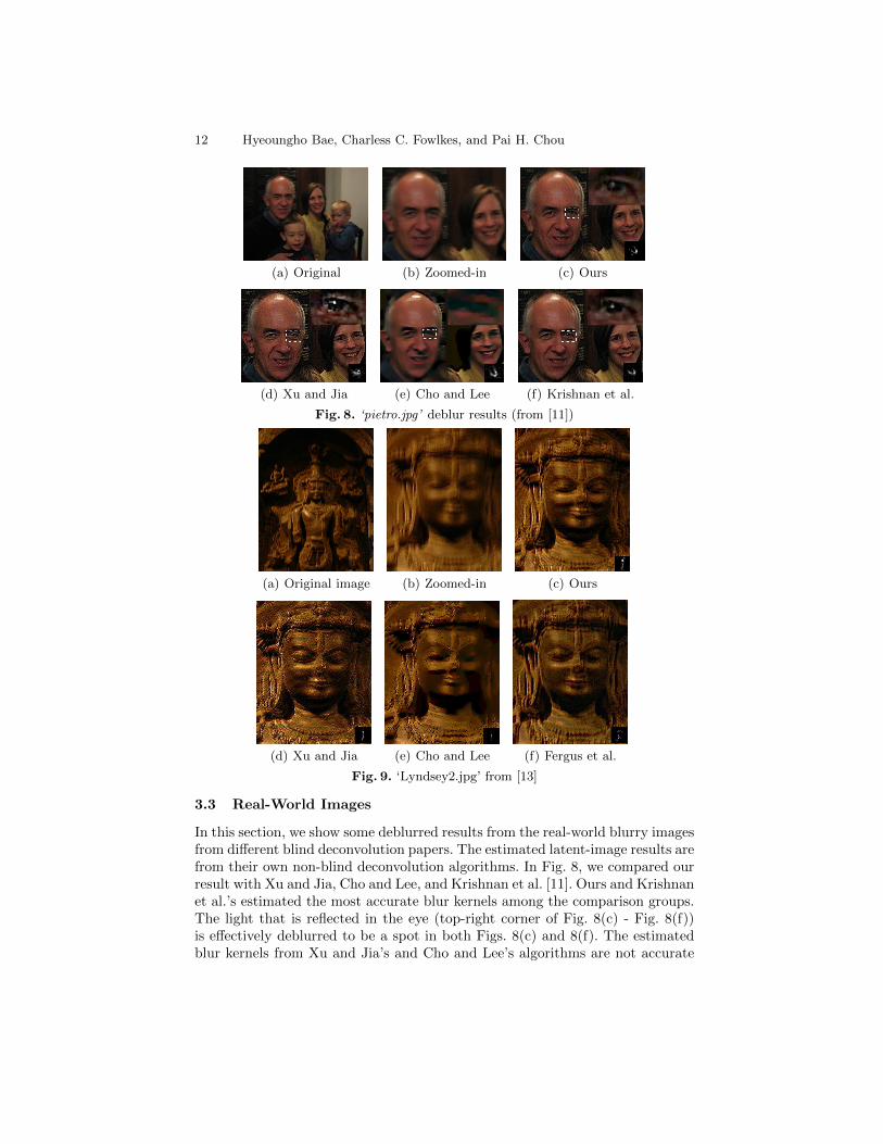
(a) Original (b) Zoomed-in (c) Ours

(d) Xu and Jia (e) Cho and Lee (f) Krishnan et al.

Fig. 8. ‘pietro.jpg’ deblur results (from [11])

(a) Original image (b) Zoomed-in (c) Ours

(d) Xu and Jia (e) Cho and Lee (f) Fergus et al.

Fig. 9. ‘Lyndsey2.jpg’ from [13]

3.3 Real-World Images

In this section, we show some deblurred results from the real-world blurry imagesfrom different blind deconvolution papers. The estimated latent-image results arefrom their own non-blind deconvolution algorithms. In Fig. 8, we compared ourresult with Xu and Jia, Cho and Lee, and Krishnan et al. [11]. Ours and Krishnanet al.’s estimated the most accurate blur kernels among the comparison groups.The light that is reflected in the eye (top-right corner of Fig. 8(c) - Fig. 8(f))is effectively deblurred to be a spot in both Figs. 8(c) and 8(f). The estimatedblur kernels from Xu and Jia’s and Cho and Lee’s algorithms are not accurate


compared to our result; the deblurred light in the eye is not a spot (Xu and Jia’sresult shown in Fig. 8(d)) or unobservable (Cho and Lee’s result in Fig. 8(e)).

In Fig. 9, we compare our result with those of Xu and Jia, Cho and Lee, andFergus et al. using the image from [13]. The estimated blur kernels are shown atthe right-bottom side of each image. In this case, Cho and Lee’s algorithm showsa preference to ‘no-blur’ result in their kernel estimation. Moreover, the latentimage shows some loss of edges. On the other hand, the result of Xu and Jiashows larger noise compared to other results. Considering their estimated kernelis similar to ours, the artifact can be attributed to their non-blind deconvolutionalgorithm.

3.4 Patch Mosaic as a General Framework

To show that our patch mosaic can be used to reduce the computation time ofother motion deblurring algorithms, we selected Krishnan et al’s algorithm [9]4.We used the approach illustrated in Fig. 1(a). The image that is fed into theestimation algorithm is synthesized by the patch mosaic algorithm for every stepof the coarse-to-fine iteration of their algorithm. The performance of the modifiedalgorithm is shown in Fig. 5 and 6. On average, the modified algorithm is 4.7times faster than the original algorithm with the cost of 17.8% increased errorratio. The average error ratio of the modified algorithm is 2.13, which is slightlyhigher than the original algorithm of 1.81 (see Krishnan (org.) vs. Krishnan(mod.) in Figs. 5(a) and 6(b)). However, the computation time of the modifiedone is only 209 sec compared to 980 sec of the original algorithm.

4 Conclusions

We propose the patch mosaic and a fast, accurate deblurring algorithm based onthe patch mosaic for spatially invariant blur-kernel estimation. A MATLAB im-plementation of our deblurring algorithm runs 4.7 times faster than the nearestcompetitor (the C++ binary of [2]) when estimating a latent image of 2256×1504pixels. Our algorithm achieves equal or better accuracy than other algorithmspublished to date. The patch mosaic can not only improve the computationtime but also exclude saturated and uniform image regions that typically mis-lead the estimation process [4, 13]. We also show that the patch mosaic can beused for other deblurring algorithms to reduce the computation time with min-imal loss of the estimation accuracy. The time analysis shows that our patchmosaic-based algorithm can effectively reduce the computation time with min-imal overhead. Since more than 40% of the time in the estimation loop is usedfor the latent image prediction, faster filtering solutions may yield further in-creases in computation speed [19]. Our algorithm may also be combined withexternal sensors to further reduce the computation time and provide strongerpriors [20]. For example, a triaxial accelerometer can be used to aid the image

4 http://cs.nyu.edu/~dilip/research/blind-deconvolution/


patch locating algorithm to focus on the edges sensitive to the direction of themotion detected by the sensor. Our algorithmic ideas can also be extended tosolving for more complex spatially variant blur-kernel estimation problems in atimely manner [10].

Acknowledgement. This work was sponsored by the National Science Foun-dation grant CBET-0933694 and Air Force Office of Scientific Research grantFA9550-10-1-0538. Any opinions, findings, and conclusions or recommendationsexpressed in this material are those of the authors and do not necessarily reflectthe views of the National Science Foundation.

References

1. Levin, A., Weiss, Y., Durand, F., Freeman, W.T.: Efficient marginal likelihoodoptimization in blind deconvolution. CVPR (2011)

2. Cho, S., Lee, S.: Fast motion deblurring. ACM Transactions on Graphics 28 (2009)3. Shan, Q., Jia, J., Agarwala, A.: High-quality motion deblurring from a single

image. ACM Transactions on Graphics 27 (2008)4. Xu, L., Jia, J.: Two-phase kernel estimation for robust motion deblurring. ECCV

(2010) 157–1705. Jia, J.: Single image motion deblurring using transparency. CVPR (2007)6. Joshi, N., Szeliski, R., Kriegman, D.: Psf estimation using sharp edge prediction.

CVPR (2008)7. Yuan, L., Sun, J., Quan, L., Shum, H.: Image deblurring with blurred/noisy image

pairs. ACM Transactions on Graphics 26 (2007)8. Cho, T.: Motion blur removal from photographs. M.I.T Ph.D dissertation (2010)9. Krishnan, D., Fergus, R.: Fast image deconvolution using hyper-laplacian priors.

Neural Information Processing Systems (2009)10. Gupta, A., Joshi, N., Zitnick, L., Cohen, M., Curless, B.: Single image deblurring

using motion density functions. In: ECCV ’10: Proceedings of the 10th EuropeanConference on Computer Vision. (2010)

11. Krishnan, D., Tay, T., Fergus, R.: Blind deconvolution using a normalized sparsitymeasure. CVPR (2011)

12. Wang, Y., Yang, J., Yin, W., Zhang, Y.: A new alternating minimization algorithmfor total variation image reconstruction. SIAM Journal of Imaging Science 1 (2009)

13. Fergus, R., Singh, B., Hertzmann, A., Roweis, S.T., Freeman, W.T.: Removingcamera shake from a single photograph. ACM Transactions on Graphics 25 (2006)

14. Bracewell, R.N.: The Fourier Transform and Its Applications. McGraw-Hill (1999)15. Levin, A., Fergus, R., Durand, F., Freeman, W.T.: Deconvolution using natural im-

age priors. http://groups.csail.mit.edu/graphics/CodedAperture /SparseDeconv-LevinEtAl07.pdf (2007)

16. Levin, A., Weiss, Y., Durand, F., Freeman, W.T.: Understanding and evaluatingblind deconvolution algorithms. CVPR (2009)

17. Richardson, W.H.: Bayesian-based iterative method of image restoration. Journalof Optics (1972)

18. Lucy, L.B.: An iterative technique for the rectification of observed distributions.Astronomical Journal (1974)

19. Yang, Q., Tan, K., Ahuja, N.: Real-time o(1) bilateral filtering. CVPR (2009)20. Joshi, N., Kang, S.B., Zitnick, C.L., Szeliski, R.: Image deblurring using inertial

measurement sensors. ACM Transactions on Graphics 29 (2010)

Documents

Patch Mosaic for Fast Motion Deblurring - ICS | UC Irvine