Int J Comput VisDOI 10.1007/s11263-014-0727-3

Deblurring Shaken and Partially Saturated Images

Oliver Whyte · Josef Sivic · Andrew Zisserman

Received: 1 May 2013 / Accepted: 25 April 2014© Springer Science+Business Media New York 2014

Abstract We address the problem of deblurring imagesdegraded by camera shake blur and saturated (over-exposed)pixels. Saturated pixels violate the common assumption thatthe image-formation process is linear, and often cause ring-ing in deblurred outputs. We provide an analysis of ringingin general, and show that in order to prevent ringing, it isinsufficient to simply discard saturated pixels. We show thateven when saturated pixels are removed, ringing is causedby attempting to estimate the values of latent pixels that arebrighter than the sensor’s maximum output. Estimating theselatent pixels is likely to cause large errors, and these errorspropagate across the rest of the image in the form of ringing.We propose a new deblurring algorithm that locates theseerror-prone bright pixels in the latent sharp image, and bydecoupling them from the remainder of the latent image,greatly reduces ringing. In addition, we propose an approx-imate forward model for saturated images, which allows us

Communicated by Dr. Srinivas Narasimhan, Dr. Frédo Durand and Dr.Wolfgang Heidrich.

Parts of this work were previously published in the IEEE Workshopon Color and Photometry in Computer Vision, with ICCV2011 Whyte et al. (2011).

O. Whyte (B)Microsoft Corporation, Redmond, WA, USAe-mail: oliverw@microsoft.com

J. SivicINRIA - Willow Project Laboratoire d’Informatique de l’EcoleNormale Supérieure (CNRS/ENS/INRIA UMR 8548),Paris, Francee-mail: josef.sivic@ens.fr

A. ZissermanVisual Geometry Group, Department of Engineering Science,University of Oxford, Oxford, UKe-mail: az@robots.ox.ac.uk

to estimate these error-prone pixels separately without caus-ing artefacts. Results are shown for non-blind deblurring ofreal photographs containing saturated regions, demonstrat-ing improved deblurred image quality compared to previouswork.

Keywords Non-blind deblurring · Saturation · Ringing ·Outliers

1 Introduction

The task of deblurring “shaken” images has received con-siderable attention recently Fergus et al. (2006); Cho andLee (2009); Gupta et al. (2010); Joshi et al. (2010); Whyteet al. (2010); Shan et al. (2008). Significant progress has beenmade towards reliably estimating the point spread function(PSF) for a given blurred image, which describes how theimage was blurred. Likewise, when the PSF for an image isknown, many authors have proposed methods to invert theblur process and recover a high quality sharp image (referredto as “non-blind deblurring”).

One problematic feature of blurred images, and in par-ticular “shaken” images, which has received relatively littleattention is the presence of saturated (over-exposed) pixels.These arise when the radiance of the scene exceeds the rangeof the camera’s sensor, leaving bright highlights clipped atthe maximum output value (e.g.255 for an image with 8 bitsper pixel). To anyone who has attempted to take hand-heldphotographs at night, such pixels should be familiar as theconspicuous bright streaks left by electric lights, such as inFig. 1a. These bright pixels, with their clipped values, violatethe assumption made by most deblurring algorithms that theimage formation process is linear, and as a result can cause

123

Int J Comput Vis

(a) (b)

(c) (d)

(a)

(b)

(c)

(d)

Fig. 1 Deblurring in the presence of saturation. Existing deblurringmethods, such as those in (b) and (c), do not take account of saturatedpixels. This leads to large and unsightly artefacts in the results, such asthe “ringing” around the bright lights in the zoomed section. Using theproposed method (d), the ringing is greatly reduced and the quality of the

deblurred image is improved. The PSF for this 1024× 768 pixel imagecauses a blur of about 35 pixels in width, and was estimated directlyfrom the blurred image using the algorithm described by Whyte et al.(2012)

obtrusive artefacts in the deblurred images. This can be seenin the deblurred images in Fig. 1b, c.

In this paper we address the problem of deblurring imagescontaining saturated pixels, offering an analysis of the arte-facts caused by existing algorithms, and a new algorithmwhich avoids such artefacts by explicitly handling saturatedpixels. Our method is applicable for all causes of blur, how-ever in this work we focus on blur caused by camera shake(motion of the camera during the exposure).

The process of deblurring an image typically involvestwo steps. First, the PSF is estimated, either using a blinddeblurring algorithm Fergus et al. (2006); Yuan et al. (2007);Shan et al. (2008); Cho and Lee (2009) to estimate the PSFfrom the blurred image itself, or by using additional hard-ware attached to the camera Joshi et al. (2010); Tai et al.(2008). Second, a non-blind deblurring algorithm is appliedto estimate the sharp image, given the PSF. In this work weaddress the second of these two steps for the case of saturatedimages, and assume that the PSF is known or has been esti-

mated already. Unless otherwise stated, all the results in thiswork use the algorithm of Whyte et al. (2011) to estimate aspatially-variant PSF. The algorithm is based on the methodof Cho and Lee (2009), and estimates the PSF directly fromthe blurred image itself. Figure 1d shows the output of theproposed algorithm, which contains far fewer artefacts thanthe two existing algorithms shown for comparison.

1.1 Related Work

Saturation has not received wide attention in the literature,although several authors have cited it as the cause of artefactsin deblurred images Fergus et al. (2006); Cho and Lee (2009);Tai et al. (2011). Harmeling et al. (2010b) address the issuein the setting of multi-frame blind deblurring by threshold-ing the blurred image to detect saturated pixels, and ignor-ing these in the deblurring process. When multiple blurredimages of the same scene are available, these pixels can be

123

Int J Comput Vis

safely discarded, since there will generally remain unsatu-rated pixels covering the same area in other images.

Recently, Cho et al. (2011) have also considered satu-rated pixels, in the more general context of non-blind deblur-ring with outliers, and propose an expectation-maximisationalgorithm to iteratively identify and exclude outliers in theblurred image. Saturated pixels are detected by blurring thecurrent estimate of the sharp image and finding places wherethe result exceeds the range of the camera. Those blurredpixels detected as saturated are ignored in the subsequentiterations of the deblurring algorithm. In Sect. 4 we discusswhy simply ignoring saturated pixels is, in general, not suf-ficient to prevent artefacts from appearing in single-imagedeblurring.

In an alternative line of work, several authors have pro-posed algorithms for non-blind deblurring that are robustagainst various types of modeling errors, without directlyaddressing the sources of those errors. Yuan et al. (2008)propose a non-blind deblurring algorithm capable of sup-pressing “ringing” artefacts during deblurring, using multi-scale regularisation. Yang et al. (2009) and Xu and Jia (2010)also consider non-blind deblurring with robust data-fidelityterms, to handle non-Gaussian impulse noise, however theirformulations do not handle arbitrarily large deviations fromthe linear model, such as can be caused by saturation.

Many algorithms exist for non-blind deblurring in thelinear (non-saturated) case, perhaps most famously theWiener filter Wiener (1949) and the Richardson–Lucy algo-rithm Richardson (1972); Lucy (1974). Recently, manyauthors have focused on the use of regularisation, derivedfrom natural image statistics, to suppress noise in the outputwhile encouraging sharp edges to appear Krishnan and Fer-gus (2009); Levin et al. (2007); Joshi et al. (2010); Afonsoet al. (2010); Tai et al. (2011); Zoran and Weiss (2011).

For the problem of “blind” deblurring, where the PSFis unknown, single-image blind PSF estimation for camerashake has been widely studied using variational and max-imum a posteriori (MAP) algorithms Fergus et al. (2006);Shan et al. (2008); Cho and Lee (2009); Cai et al. (2009); Xuand Jia (2010); Levin et al. (2011); Krishnan et al. (2011).Levin et al. (2009) review several approaches and providea ground-truth dataset for comparison on spatially-invariantblur. While most work has focused on spatially-invariant blur,several approaches have also been proposed for spatially-varying blur Whyte et al. (2010); Gupta et al. (2010); Harmel-ing et al. (2010a); Joshi et al. (2010); Tai et al. (2011).

The remainder of this paper proceeds as follows: Webegin in Sect. 2 by providing some background on non-blinddeblurring and saturation in cameras. In Sect. 3 we analysesome of the properties and causes of “ringing” artefacts(which are common when deblurring saturated images), anddiscuss the implications of this analysis in Sect. 4. Based onthis discussion, in Sect. 5 we describe our proposed approach.

We present deblurring results and comparison to related workin Sect. 6.

2 Background

In most existing work on deblurring, the observed imageproduced by a camera is modelled as a linear blur operationapplied to a sharp image, followed by a random noise process.Under this model, an observed blurred image g (written as anN × 1 vector, where N is the number of pixels in the image)can be written in terms of a (latent) sharp image f (also anN × 1 vector) as

g∗ = Af (1)

g = g∗ + ε, (2)

where A is an N × N matrix representing the discrete PSF,g∗ represents the “noiseless” blurred image, and ε is somerandom noise affecting the image. Typically, the noise ε ismodelled as following either a Poisson or Gaussian distrib-ution, independent at each pixel.

For many causes of blur, the matrix A can be parameterisedby a small set of weights w, often referred to as a blur kernel,such that

A =∑

k

wkTk, (3)

where each N × N matrix Tk applies some geometric trans-formation to the sharp image f . Classically, Tk have beenchosen to model translations of the sharp image, allowingEq. (1) to be written as a 2D convolution of f with w. Forblur caused by camera shake (motion of the camera dur-ing exposure), recent work Gupta et al. (2010); Joshi et al.(2010); Whyte et al. (2010); Tai et al. (2011) has shown thatusing projective transformations for Tk is more appropriate,and leads to more accurate modeling of the spatially-variantblur caused by camera shake. The remainder of this work isagnostic to the form of A, and thus can be applied equally tospatially-variant and spatially-invariant blur.

Non-blind deblurring (where A is known) is generally per-formed by attempting to solve a minimisation problem of theform

minf

L(g, Af)+ αφ(f), (4)

where the data-fidelity term L penalises sharp images thatdo not closely fit the observed data (i.e.L is a measure of“distance” between g and Af), and the regularisation termφ penalises sharp images that do not adhere to some priormodel of sharp images. The scalar weight α balances thecontributions of the two terms in the optimisation.

123

Int J Comput Vis

In a probabilistic setting, where the random noise ε isassumed to follow a known distribution, the data-fidelity termcan be derived from the negative log-likelihood:

L(g, Af) = − log p(g|Af), (5)

where p(g|Af) denotes the probability of observing theblurry image g, given a sharp image f and PSF A (oftenreferred to as the likelihood). If the noise follows pixel-independent Gaussian distributions with uniform variance,the appropriate data-fidelity term is

LG(g, Af) =∑

i

(gi − (Af)i

)2, (6)

where (Af)i indicates the i th element of the vector Af . WithGaussian noise, Eq. (4) is typically solved using standardlinear least-squares algorithms, such as conjugate gradientdescent Levin et al. (2007). For the special case of spatially-invariant blur, and provided that the regularisation term φ

can also be written as a quadratic function of f , Eq. (4) has aclosed-form solution in the frequency domain, which can becomputed efficiently using the fast Fourier transform Wiener(1949); Gamelin (2001).

If the noise follows a Poisson distribution, the appropriatedata-fidelity term is

LP(g, Af) = −∑

i

(gi log(Af)i − (Af)i

). (7)

The classic algorithm for deblurring images with Poissonnoise is the Richardson–Lucy algorithm Richardson (1972);Lucy (1974), an iterative algorithm described by a simplemultiplicative update equation. The incorporation of regu-larisation terms into this algorithm has been addressed byTai et al. (2011) and Welk (2010). We discuss this algorithmfurther in Sect. 5.

A third data-fidelity term that is more robust to outliersthan the two mentioned above, and which has been appliedfor image deblurring with impulse noise is the �1 norm Baret al. (2006); Yang et al. (2009) (corresponding to noise witha Laplacian distribution):

LL(g, Af) =∑

i

∣∣gi − (Af)i∣∣. (8)

Although this data-fidelity term is more robust against noisevalues εi with large magnitudes, compared to the Gaussianor Poisson data-fidelity terms, it still produces artefacts in thepresence of saturation Cho et al. (2011).

For clarity, in the remainder of the paper we denote thedata-fidelity term L(g, Af) simply as L(f), since we considerthe blurred image g and the PSF matrix A to be fixed.

2.1 Sensor Saturation

Sensor saturation occurs when the radiance of the scenewithin a pixel exceeds the camera sensor’s range, at whichpoint the sensor ceases to integrate the incident light, andproduces an output that is clamped to the largest outputvalue. This introduces a non-linearity into the image for-mation process that is not modelled by Eqs. (1) and (2).To correctly describe this effect, our model must include anon-linear function R, which reflects the sensor’s non-linearresponse to incident light. This function is applied to eachpixel of the image before it is output by the sensor, i.e.

gi = R(g∗i + εi

), (9)

where εi represents the random noise on pixel i .For the purpose of describing saturation, we model the

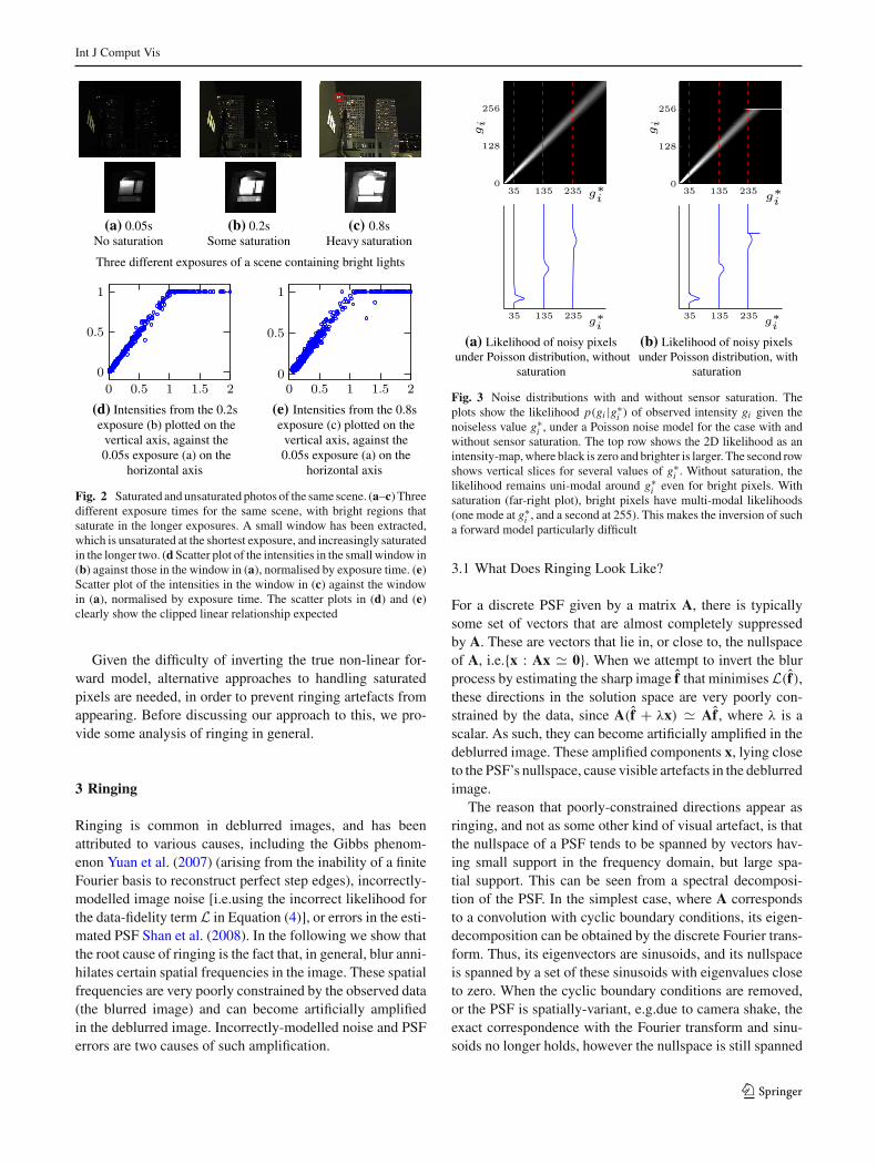
non-linear response function R as a truncated linear function,i.e.R(x) = min(x, 1), for intensities scaled to lie in the range[0, 1]. This model is supported by the data in Fig. 2, whichshows the relationship between pixel intensities in three dif-ferent exposures of a bright light source. The pixel values inthe short exposure (with no saturation) and the longer expo-sures (with saturation) clearly exhibit this clipped linear rela-tionship. As the length of the exposure increases, more pixelssaturate.

Due to the non-linearity in the image formation process,simply applying existing methods for non-blind deblur-ring (which assume a linear image formation model) toimages affected by saturation, produces deblurred imageswhich exhibit severe artefacts in the form of “ringing” –medium frequency ripples that spread across the image, e.g.inFig. 1b, c. Clearly, the saturation must be taken into accountduring non-blind deblurring in order to avoid such arte-facts.

Given the non-linear forward model in Eq. (9), it is tempt-ing to modify the data-fidelity term L to take into accountsaturation, and thus prevent artefacts from appearing in thedeblurred image. The model in Eq. (9), however, is nottractable to invert. Since the noise term εi lies inside R, thelikelihood p(gi |g∗i ) (from which L is derived) is distortedand, in general, can no longer be written in closed-form.Figure 3 shows the difference between the likelihoods withand without saturation for Poisson noise. In the saturatedlikelihood, pixels near the top of the camera’s range havedistributions that are no longer smooth and uni-modal, butinstead have a second sharp peak at 1. Furthermore, for somepixels this second mode at 1 is the maximum of the likelihood,i.e.P(gi = 1|g∗i ) > P(gi = g∗i |g∗i ), which clearly contra-dicts the normal behaviour of Poisson or Gaussian noise,where the likelihood is smooth and has a single mode atgi = g∗i .

123

Int J Comput Vis

(a) (b) (c)

(d) (e)

Fig. 2 Saturated and unsaturated photos of the same scene. (a–c) Threedifferent exposure times for the same scene, with bright regions thatsaturate in the longer exposures. A small window has been extracted,which is unsaturated at the shortest exposure, and increasingly saturatedin the longer two. (d Scatter plot of the intensities in the small window in(b) against those in the window in (a), normalised by exposure time. (e)Scatter plot of the intensities in the window in (c) against the windowin (a), normalised by exposure time. The scatter plots in (d) and (e)clearly show the clipped linear relationship expected

Given the difficulty of inverting the true non-linear for-ward model, alternative approaches to handling saturatedpixels are needed, in order to prevent ringing artefacts fromappearing. Before discussing our approach to this, we pro-vide some analysis of ringing in general.

3 Ringing

Ringing is common in deblurred images, and has beenattributed to various causes, including the Gibbs phenom-enon Yuan et al. (2007) (arising from the inability of a finiteFourier basis to reconstruct perfect step edges), incorrectly-modelled image noise [i.e.using the incorrect likelihood forthe data-fidelity term L in Equation (4)], or errors in the esti-mated PSF Shan et al. (2008). In the following we show thatthe root cause of ringing is the fact that, in general, blur anni-hilates certain spatial frequencies in the image. These spatialfrequencies are very poorly constrained by the observed data(the blurred image) and can become artificially amplifiedin the deblurred image. Incorrectly-modelled noise and PSFerrors are two causes of such amplification.

(a) (b)

Fig. 3 Noise distributions with and without sensor saturation. Theplots show the likelihood p(gi |g∗i ) of observed intensity gi given thenoiseless value g∗i , under a Poisson noise model for the case with andwithout sensor saturation. The top row shows the 2D likelihood as anintensity-map, where black is zero and brighter is larger. The second rowshows vertical slices for several values of g∗i . Without saturation, thelikelihood remains uni-modal around g∗i even for bright pixels. Withsaturation (far-right plot), bright pixels have multi-modal likelihoods(one mode at g∗i , and a second at 255). This makes the inversion of sucha forward model particularly difficult

3.1 What Does Ringing Look Like?

For a discrete PSF given by a matrix A, there is typicallysome set of vectors that are almost completely suppressedby A. These are vectors that lie in, or close to, the nullspaceof A, i.e.{x : Ax � 0}. When we attempt to invert the blurprocess by estimating the sharp image f that minimises L(f),these directions in the solution space are very poorly con-strained by the data, since A(f + λx) � Af , where λ is ascalar. As such, they can become artificially amplified in thedeblurred image. These amplified components x, lying closeto the PSF’s nullspace, cause visible artefacts in the deblurredimage.

The reason that poorly-constrained directions appear asringing, and not as some other kind of visual artefact, is thatthe nullspace of a PSF tends to be spanned by vectors hav-ing small support in the frequency domain, but large spa-tial support. This can be seen from a spectral decomposi-tion of the PSF. In the simplest case, where A correspondsto a convolution with cyclic boundary conditions, its eigen-decomposition can be obtained by the discrete Fourier trans-form. Thus, its eigenvectors are sinusoids, and its nullspaceis spanned by a set of these sinusoids with eigenvalues closeto zero. When the cyclic boundary conditions are removed,or the PSF is spatially-variant, e.g.due to camera shake, theexact correspondence with the Fourier transform and sinu-soids no longer holds, however the nullspace is still spanned

123

Int J Comput Vis

(a) (b)

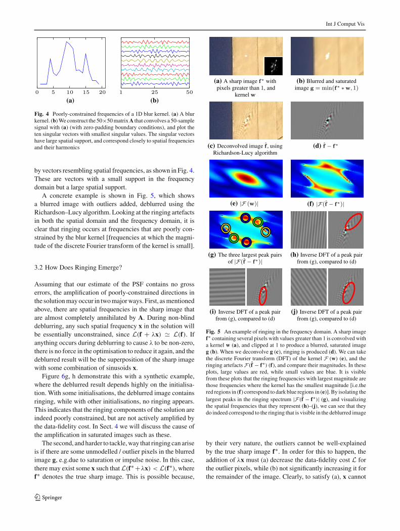
Fig. 4 Poorly-constrained frequencies of a 1D blur kernel. (a) A blurkernel. (b) We construct the 50×50 matrix A that convolves a 50-samplesignal with (a) (with zero-padding boundary conditions), and plot theten singular vectors with smallest singular values. The singular vectorshave large spatial support, and correspond closely to spatial frequenciesand their harmonics

by vectors resembling spatial frequencies, as shown in Fig. 4.These are vectors with a small support in the frequencydomain but a large spatial support.

A concrete example is shown in Fig. 5, which showsa blurred image with outliers added, deblurred using theRichardson–Lucy algorithm. Looking at the ringing artefactsin both the spatial domain and the frequency domain, it isclear that ringing occurs at frequencies that are poorly con-strained by the blur kernel [frequencies at which the magni-tude of the discrete Fourier transform of the kernel is small].

3.2 How Does Ringing Emerge?

Assuming that our estimate of the PSF contains no grosserrors, the amplification of poorly-constrained directions inthe solution may occur in two major ways. First, as mentionedabove, there are spatial frequencies in the sharp image thatare almost completely annihilated by A. During non-blinddeblurring, any such spatial frequency x in the solution willbe essentially unconstrained, since L(f + λx) � L(f). Ifanything occurs during deblurring to cause λ to be non-zero,there is no force in the optimisation to reduce it again, and thedeblurred result will be the superposition of the sharp imagewith some combination of sinusoids x.

Figure 6g, h demonstrate this with a synthetic example,where the deblurred result depends highly on the initialisa-tion. With some initialisations, the deblurred image containsringing, while with other initialisations, no ringing appears.This indicates that the ringing components of the solution areindeed poorly constrained, but are not actively amplified bythe data-fidelity cost. In Sect. 4 we will discuss the cause ofthe amplification in saturated images such as these.

The second, and harder to tackle, way that ringing can ariseis if there are some unmodelled / outlier pixels in the blurredimage g, e.g.due to saturation or impulse noise. In this case,there may exist some x such that L(f∗ +λx) < L(f∗), wheref∗ denotes the true sharp image. This is possible because,

(d)

(e) (f)

(a) (b)

(c)

(g) (h)

(i) (j)

Fig. 5 An example of ringing in the frequency domain. A sharp imagef∗ containing several pixels with values greater than 1 is convolved witha kernel w (a), and clipped at 1 to produce a blurred, saturated imageg (b). When we deconvolve g (c), ringing is produced (d). We can takethe discrete Fourier transform (DFT) of the kernel F (w) (e), and theringing artefacts F(f − f∗) (f), and compare their magnitudes. In theseplots, large values are red, while small values are blue. It is visiblefrom these plots that the ringing frequencies with largest magnitude arethose frequencies where the kernel has the smallest magnitude [i.e.thered regions in (f) correspond to dark blue regions in (e)]. By isolating thelargest peaks in the ringing spectrum |F(f − f∗)| (g), and visualizingthe spatial frequencies that they represent (h)–(j), we can see that theydo indeed correspond to the ringing that is visible in the deblurred image

by their very nature, the outliers cannot be well-explainedby the true sharp image f∗. In order for this to happen, theaddition of λx must (a) decrease the data-fidelity cost L forthe outlier pixels, while (b) not significantly increasing it forthe remainder of the image. Clearly, to satisfy (a), x cannot

123

Int J Comput Vis

(a) (b) (c) (d)

(e) (f) (g) (h)

Fig. 6 Synthetic example of deblurring with saturated pixels. (a) Asharp image f∗ containing some bright pixels with intensity twice themaximum image value. (b) The sharp image f is convolved with w andclipped at 1 to simulate saturation. No noise is added in this example.(c) The mask of pixels in g that are not saturated, i.e.mi = 1 (white) if(f∗ ∗ w)i < 1, and mi = 0 (black) otherwise. (d) The mask of pixelsin g that are not influenced by the bright pixels in f∗, i.e.mi = 1 if((f∗ ≥ 1) ∗ w

)i = 0. See Sect. 5.1 for further explanation. The fol-

lowing rows show the results of deblurring g with 1000 iterations ofthe Richardson–Lucy algorithm, starting from three different initialisa-tions. (1st row) initialised with blurred image. (2nd row) initialised with

random values in [0, 1]. (3rd row) initialised with true sharp image. Ascan be seen, in (f), ringing appears regardless of the initialisation, indi-cating that L is encouraging this to occur. In (g), ringing appears withsome initialisations but not others, indicating that L does not encourageit, but does not suppress it either. In (h), ringing is almost gone, since wehave removed the most destabilising data. Counterintuitively, althoughwe have discarded more data, we end up with less ringing. Note that byremoving all the blurred pixels shown in (d), we have no informationabout the bright pixels in f , and they simply retain their initial values.Note also that the deblurred images f may contain pixel values greaterthan 1, however they are clamped to 1 before writing the image to file

lie exactly in the nullspace of A, otherwise Ax = 0, howeverto satisfy (b), it also cannot lie too far from the nullspace,otherwise the data-fidelity cost would grow quickly with λ.The result is that x lies close to, but not in, the nullspace ofA, and the optimisation is more-or-less free to change λ inorder to explain the outliers more accurately.

Figure 6f shows an example of this, where for all initiali-sations, some ringing appears, and the deblurred image f hasa lower data-fidelity cost than the true sharp image f∗. Notethat the ringing in Fig. 6f is visually similar to that in Fig. 6g,h, underlining the fact that in both cases, ringing appears inthe poorly-constrained frequencies of the result.

One additional way that ringing may emerge in a deblurredimage, which we do not address in this work, is if the PSF is

incorrectly estimated. In this case, the PSF used to debluris different from the one which caused the blur, and thedeblurred image will be incorrect due to this discrepancy. Wedo not go into detail here, but for an estimated PSF A thatis related to the true PSF A by A = A+�A, the deblurredimage will contain ringing in the spatial frequencies where

A has a small frequency response (i.e.close to the null-space of A) Whyte (2012). This echoes the conclusions ofthe previous paragraphs, with the difference that the ringingfrequencies are determined by the incorrect PSF A, instead ofthe true PSF A. The problem of deblurring with an erroneousPSF has also been addressed recently by Ji and Wang (2012),who introduce additional latent variables in order to estimatef in a manner that is invariant to a certain class of PSF errors.

123

Int J Comput Vis

3.3 Why Doesn’t Regularisation Suppress Ringing?

Often, ringing appears in deblurred images despite the inclu-sion of some regularisation term φ in the optimisation prob-lem in Eq. (4). This seems counterintuitive, since the purposeof the regularisation is to provide some additional constraintson the solution, particularly in directions which are poorlyconstrained by the data.

However, most popular forms of regularisation used innon-blind deblurring penalise only the magnitudes of the firstor second spatial derivatives of the deblurred image, e.g.

φ(f) =∑

i

ρ(|(dx ∗ f)i |

)+ ρ(|(dy ∗ f)i |

), (10)

where the sum is taken over all pixels i in the image, the fil-ters dx and dy compute derivatives, and ρ is a non-decreasingscalar function Blake and Zisserman (1987); Bouman andSauer (1993); Schultz and Stevenson (1994); Levin et al.(2007). These derivatives are computed from the differencesbetween neighbouring pixels, and are essentially high-passfilters. Unsurprisingly, such regularisation works best at sup-pressing high spatial frequencies. At medium-to-low fre-quencies, the power of the regularisation decreases.

Figure 7 demonstrates this, showing how the power ofthe regularisation is greatest at high frequencies, and falls tozero at low frequencies . The blurred data on the other handconstrains the lowest frequencies (i.e.at scales larger thanthe blur), but not the high frequencies. There is a region ofmedium frequencies that are poorly constrained by both. Itis at these intermediate frequencies that some ringing x caneasily appear, since L(f∗ + λx) � L(f∗), and φ(f∗ + λf) �φ(f∗). Although the regularisation weight α in Eq. (4) canbe increased in order to reduce ringing, this will also beginto over-smooth the deblurred image.

Yuan et al. (2008) observe this fact and propose a multi-scale non-blind deblurring algorithm capable of preventingringing caused by noise and numerical inaccuracies . How-ever, although their method can suppress ringing at a widerange of frequencies, it is still generally unable to handleringing caused by saturation, as shown in Fig. 13.

4 Preventing Ringing when Deblurring SaturatedImages

When applying existing non-blind deblurring algorithms tosaturated images, which assume the linear model g = Af+ε,using Gaussian or Poisson data-fidelity terms L, ringing isalmost certain to appear. As discussed in the previous section,saturated pixels can cause the phenomenon where a deblurredimage f containing ringing actually has a lower data-fidelity

Fig. 7 Power spectra of blur and gradient filters. The power spectrumof the 1D blur kernel in Fig. 4 (solid blue line), and the power spec-trum of the derivative filter [1,−1] (dashed red line), often used forregularisation in non-blind deblurring. The blur kernel has minima inits power spectrum, which correspond to poorly-constrained frequen-cies in the deblurred solution. At the low-frequency minima (e.g.near5 cycles/image), the gradient filter has also lost most of its power, andso ringing at these frequencies is unlikely to be suppressed by gradient-based regularisation (Color figure online)

cost than the true sharp image f∗, due to the fact that theassumption of linearity is violated.

Although the saturation can be modelled with a non-linearresponse R (as discussed in Sect. 2.1) in order to prevent thecase where L(f∗ + λx) < L(f∗), the model is not tractableto invert. For this reason, some recent authors have insteadchosen to treat saturated pixels simply as outliers, and modelthe rest of the image as linear Harmeling et al. (2010b); Choet al. (2011). The saturated pixels are discarded and treatedas missing data. Not only is this much more tractable to opti-mise, it arguably does not sacrifice much – saturated pixelsare largely uninformative, due to being clamped at the max-imum output value.

In order to perform non-blind deblurring with missingdata, we can define a mask m of binary weights, wheremi = 0 if pixel i is missing, and mi = 1 otherwise. We thenconstruct a weighted form of the data-fidelity term, using mas the weights, and denote this Lm. For example, for Poissonnoise, Eq. (7) becomes:

LPm(f) = −

∑

i

mi(gi log(Af)i − (Af)i

). (11)

By removing all the data that does not follow the linearmodel, it should no longer be possible for Lm(f∗ + λx) <

Lm(f∗).Harmeling et al. (2010b) estimate the mask m directly

from the blurred image, by finding all the pixels in g that are

123

Int J Comput Vis

above some threshold ϕ close to 1, i.e.

mi ={

1 if gi < ϕ

0 otherwise.(12)

On the other hand, Cho et al. (2011) estimate m by blurringthe current estimate of the sharp image f :

mi ={

1 if (Af)i < 1

0 otherwise.(13)

Note that although some of the blurred pixels are discarded,the entire latent image f is still estimated.

Although detecting and ignoring the (outlier) saturatedpixels can reduce ringing in the deblurred images, it does notnecessarily remove it entirely. By discarding saturated data,the data-fidelity term Lm no longer actively encourages ring-ing. However, it may still be possible that Lm(f∗ + λx) �Lm(f∗) for some ringing x. As discussed in the previoussection, if anything in the data, the initialisation, or in thedeblurring algorithm serves to increase λ, there is no force toreduce it again, and the ringing will appear in the final result.Figure 6g demonstrates this with a synthetic example. Evenwhen the outliers are known exactly, and are completelyremoved from the deblurring process, ringing can still appear.On the other hand, when we initialise the deblurring algo-rithm with the true sharp image, no ringing appears, indicat-ing that there is nothing about Lm that causes ringing, thereis simply nothing to prevent or suppress it.

From this discussion, we conclude that in order to deblursaturated images without introducing ringing, we must domore than simply remove the saturated pixels from theobserved image g. We must also avoid amplifying the poorly-constrained spatial frequencies in the latent image f . Toachieve this, we could either introduce some form of regular-isation to place additional constraints on f , such as in Yuanet al. (2008), or we could directly modify the data-fidelityterm. In this work we choose the latter approach, eschew-ing the use of regularisation to prevent ringing (although werevisit regularisation later in order to reduce other sources ofnoise in the deblurred results).

In this work, we posit that for the case of saturation, themain factor causing poorly-constrained spatial frequenciesto become amplified is that there exist pixels in the sharpimage that exceed the image’s range, i.e.∃ j : f j > 1. Dur-ing non-blind deblurring, we must estimate these “bright”pixels’ values, and it is the act of estimating these valuesthat destabilises our estimates of other pixels. Note thatremoving the saturated pixels from g does not, in general,remove the influence of these “bright” latent pixels fromthe blurred image; a latent pixel with intensity greater than1 can contribute to a blurred pixel whose intensity is less

than 1. Indeed, a blurred image with no saturation at all maystill correspond to a latent image containing pixels brighterthan 1.

When we attempt to estimate a “bright” pixel’s value f j ,we are likely to make a relatively inaccurate estimate. Themain reason for this is that the set of observations (blurredpixels) concerning f j is likely to be incomplete. In the blur-ring process, each latent pixel in the sharp image is spreadacross multiple pixels in the blurred image g. Given thatf j > 1, there is a good chance that some of these blurredpixels will be saturated, and thus uninformative as to thevalue of f j . With fewer observations from which to estimatef j , its value will be more susceptible to noise, and containlarger error than if we had a full set of unsaturated observa-tions available. This is supported by Fig. 6g, where the sharpimage contains pixels with intensity greater than 1, and theappearance of ringing depends on the initialisation. When weinitialise with the true sharp image, which already containsthe bright (> 1) pixels, no ringing is caused. When we ini-tialise with the blurred image, or random values in [0, 1], thealgorithm is forced to attempt to estimate the bright values,and in doing so causes ringing.

Since this amplification is caused when we attempt to esti-mate the “bright” pixels in f , our approach to preventing ring-ing is based on the idea that we should avoid (or rather, delay)estimating such bright pixels. If we only estimate pixels thatcan be accurately estimated, we will not make gross errors,which in turn will avoid introducing ringing. For the syn-thetic example, Fig. 6h shows the result of this approach. Byrefusing to estimate the bright (> 1) pixels in f , the ringingis almost removed for all initialisations. In the next sectionwe discuss how we do this in practice.

Note that this idea is similar to the notion of “HighestConfidence First” Chou and Brown (1990). Chou and Brownpoint out that due to the coupling of pixels in a Markov Ran-dom Field image model, the estimate for a pixel with strongobservations may be negatively impacted by a poor deci-sion at a neighbouring pixel with weak observations. In suchcases, the pixel with strong observations “can do better with-out the incorrect information of a neighbor.”

5 Proposed Method

In this section we describe our proposed algorithm for deblur-ring images containing saturated pixels. We begin by describ-ing our approach to estimating the latent image without intro-ducing ringing, motivated by the discussion in the previoussections. In addition, we propose a method for estimatingthe bright pixels separately, without introducing artefacts,and finally describe how these elements are combined intothe complete proposed method.

123

Int J Comput Vis

5.1 Preventing Ringing by Refusing to Make Bad Estimates

As we have seen, it is clear that when we attempt to performnon-blind deblurring on an image containing saturation, wewill incorrectly estimate the “bright” latent pixels (with val-ues close to or greater than 1) that caused the saturation. Asdiscussed in the previous section, the errors we make at thesebright pixels will cause ringing. In this section we propose amethod that iteratively attempts to classify these latent pix-els, and remove them from the estimation process, therebymitigating their effect on the rest of the image.

Assume for now that we already know which pixels in thelatent image are bright, and will thus be poorly estimated. Wedenote this set of pixels S, and denote its set complement(containing the rest of the image, which can be estimatedaccurately) by U . We can write the latent image in terms ofthese two disjoint sets: f = fU + fS .

Given that we are unable to estimate fS accurately, ouraim is to prevent the propagation of errors from fS to fU . Toachieve this, we decouple our estimate of fU from our esti-mate of fS . First, note that we can decompose the noiselessblurred image as:

g∗ = AfU + AfS . (14)

We denote by V the set of blurred pixels that are not affectedby fS , i.e.V = {

i∣∣(AfS)i = 0

}, and construct the corre-

sponding binary mask v (where vi = 1 if i ∈ V , and vi = 0otherwise). Then, given that v ◦ AfS = 0, we can write

v ◦ g∗ = v ◦ AfU (15)

where · ◦ · represents the element-wise product between twovectors. From this, we can estimate fU independently of fS .Note that we can obtain the mask v simply by constructing thebinary mask u that corresponds to the set U , and performinga binary erosion of u with the non-zeros of the PSF.

Furthermore, given that the set U does not contain anybright latent pixels, AfU should not cause any saturation.Thus, we can estimate fU without modelling the non-linearitycaused by saturation, and write the observed blurred image,including noise, as

v ◦ g = v ◦ AfU + v ◦ ε. (16)

To estimate fU from v ◦ g, we can adapt existing non-blind deblurring algorithms to handle missing data, as seenin Sect. 4. For Poisson noise, the data-fidelity term is sim-ply weighted, as in Eq. (11), using v as the weights to formLP

v . The classical algorithm for non-blind deblurring withPoisson noise is the Richardson–Lucy algorithm, which is

described by the multiplicative update equation:

f t+1 = f t ◦ A�(

g

Af t

), (17)

where the division is performed element-wise.We can adapt the Richardson–Lucy update equation from

Eq. (17) to minimise the binary-weighted data-fidelity termLP

v , instead of the homogeneous LP, leading to the followingupdate equation for fU :

f t+1U = f t

U ◦ A�(

g ◦ v

Af tU+ 1− v

). (18)

Note that in order to avoid division by zero, we add a smallpositive constant to the denominator of the fraction.

This update equation is applicable to any kind of missingdata in g, the important distinction is in how we determine v,the mask of missing pixels. In Fig. 6h, we show the result ofdeblurring with v determined as described above, by erodingu. For comparison, Fig. 6g shows the result when v is deter-mined simply by finding saturated pixels in g, i.e.vi = 1 ifgi < 1. Despite removing all the saturated pixels, the resultsin Fig. 6g still contain ringing, while significantly less ringingappears in Fig. 6h using the proposed approach.

5.2 Preventing Artefacts Inside Bright Regions

While the update method in the previous section is effectiveat preventing ringing from propagating outwards from brightregions into other parts of the image, we still wish to estimatevalues for the pixels in S. Since these pixels are bright, andunlikely to be estimated accurately, we are not concernedwith preventing propagation of information from U to S,and choose to update them using all the available data.

Using the standard Richardson–Lucy update for thesebright regions however, can cause dark artefacts to appear,due to the fact that the linear model cannot explain the sat-urated data. Such artefacts are visible in Fig. 10d. To pre-vent these artefacts, we propose a second modification of theRichardson–Lucy algorithm, to include a non-linear responsefunction. Since the true forward model, discussed in Sect. 2.1is not tractable to invert, we propose the following tractablebut approximate alternative, which is sufficient for prevent-ing artefacts in bright regions:

gi = R(g∗i )+ εi , (19)

where now the response R function comes before the noise.Re-deriving the Richardson–Lucy algorithm with this model

123

Int J Comput Vis

Fig. 8 Modelling the saturated sensor response. Smooth and differen-tiable approximation to the non-differentiable function min(x, 1) usedto model sensor saturation, defined in Eq. (21). The derivative is alsosmooth and defined everywhere

gives the following update equation for the pixels in S:

f t+1S = f t

S ◦ A�(

g ◦ R′(Af t )

R(Af t )+ 1− R′(Af t )

), (20)

where R′(·) indicates the derivative of the response functionR.

Since the ideal response function R(x) = min(x, 1) isnot differentiable, we use a smooth, continuously differen-tiable approximation to this function Chen and Mangasarian(1996), where

R(x) = x − 1

alog

(1+ exp

(a(x − 1)

))(21)

R′(x) = 1

1+ exp(a(x − 1)

) . (22)

The parameter a controls the smoothness of the approxima-tion, and we have found a = 50 to be a suitable compromisebetween smoothness and accuracy (we use this value in allresults presented in this paper). Figure 8 shows the shape ofthese smooth versions of R and R′.

Equation (20) can be roughly interpreted as weightingthe blurry pixels according to the value of R′: in the linear(unsaturated) portion where x < 1, R(x) � x and R′(x) � 1,so that the term in parentheses is the same as for the standardRL algorithm. In the saturated portion where x > 1, R(x) �1 and R′(x) � 0, so that the term in parentheses is equal tounity and has no influence on f . We note that this behaviouris very similar to the method used by Cho et al. (2011) tohandle saturation – given the current estimate f of the sharpimage, they compute the blurred estimate Af , and ignore anyblurry pixel i for which (Af)i > 1.

5.3 Segmenting the Latent Image

So far in this section, we have assumed that S and U areknown. Given a real blurred image however, we do not knowa priori which parts of f belong in U and which in S. We thustreat U as another latent variable, in addition to the latentimage f , and perform the segmentation at each iteration t .Given the discussion in previous sections, we adopt a sim-ple segmentation process, which consists of thresholding thelatent image at some level ϕ close to 1:

U = {j∣∣ f t

j ≤ ϕ}. (23)

We decompose f t according to

f tU = u ◦ f t (24)

f tS = f t − f t

U , (25)

where u is the binary mask corresponding to U . Since our aimis to ensure that no large errors are introduced in fU , we setthe threshold low enough that most potentially-bright pixelsare assigned to S. Empirically, we choose ϕ = 0.9 for theresults in this paper, although we have not found the resultsto be particularly sensitive to the exact value of ϕ.

5.4 Adding Regularisation

Although the focus of this work is mitigating ringing by mod-ifying the data-fidelity term, rather than by designing newforms of regularisation, it may nonetheless still be usefulto apply some form of regularisation to reduce other noisethroughout the deblurred image. As discussed by Tai et al.(2011) and Welk (2010) it is possible to include a regularisa-tion term in the Richardson–Lucy algorithm, and this remainstrue for our algorithm. In this work we include the �1-norm ofthe gradients of the deblurred image as regularisation. Usingthe form of Eq. (10), this is written

φ(f) =∑

i

∣∣(dx ∗ f)i∣∣+ ∣∣(dy ∗ f)i

∣∣, (26)

where the filters dx and dy compute derivatives.We incorporate this in the manner described by Tai et al.

(2011). Denoting the unregularised update of f as f t+1unreg (com-

puted as in Eqs. (18) and (20) of the previous sections), wecompute the update for the regularised problem as

f t+1 = f t+1unreg

1+ α∇φ(f t ), (27)

123

Int J Comput Vis

(a) (b)

(c) (d)

Fig. 9 Effect of regularisation. This figure shows a real shaken image,and the effect of our algorithm with and without regularisation. Notethat the ringing around saturated regions, visible in (b) is removed byour method (c), even without regularisation. By adding regularisation(d), the remaining noise (visible in textureless regions) is ameliorated

where ∇φ(f t ) is the vector of partial derivatives of the regu-larisation1 φ with respect to each pixel of the latent image f ,evaluated at f t , i.e.

(∇φ(f t ))

j =∂φ(f)∂ f j

∣∣∣∣f t

. (28)

In Fig. 9 we compare results obtained using our method withand without this regularisation. As can be seen, the ring-ing is largely suppressed by the steps described in the pre-ceding sections. The addition of the regularisation term fur-

1 We note that the regulariser φ in Eq. (26) is not continuously differen-tiable, however this can be avoided by using the standard approximation|x | � √ε + x2, for some small number ε.

ther improves the results by reducing noise elsewhere in thedeblurred result.

We summarise our complete proposed algorithm in Algo-rithm 1. Figure 10 shows the contributions of the two pro-posed modifications for a synthetic 1D example. As is visible,the use of the decoupled update prevents ringing from spread-ing across the deblurred result, while the use of the non-linearforward model prevents dark artefacts from appearing insidethe bright regions. By combining these two methods, we pro-duce our best estimate of the pixels in S and U , while pre-venting the errors we make in S from affecting the rest of theimage.

Algorithm 1: Proposed algorithm

DontPrintSemicolon Input: Blurred image g, blur descriptor w1

Output: Deblurred image ff0 ← g;2for t = 0 to num_iterations do3

Decompose f t into f tU and f t

S using (23) to (25);4Compute set V in the blurred image by eroding U with PSF;5

Compute f t+1U using only data from V (18);6

Compute f t+1S using all data, with non-linear modification7

(20);f t+1unreg = f t+1

U + f t+1S ;8

Compute regularised update f t+1 using (27);9

end10

5.5 Implementation

In this section we describe some of the implementationdetails of the proposed algorithm. When segmenting the cur-rent estimate of the latent image, we take additional steps toensure that we make a conservative estimate of which pix-els can be estimated accurately. First, after thresholding thelatent image in Eq. (23), we perform a binary erosion on U ,such that

U = {j∣∣ f j ≤ ϕ

}�M, (29)

where � denotes binary erosion, and the structuring ele-ment M used for erosion is a disk of radius 3 pixels. Thisensures that all poorly-estimated pixels are correctly assignedto S (perhaps at the expense of wrongly including somewell-estimated pixels too). Performing this step improvesthe deblurred results, since it is not only the bright pix-els whose value is likely to be inaccurate due to saturation,but their neighbours too. Fewer artefacts arise from wronglyassigning a well-estimated pixel into S than the other wayaround. Second, in order to avoid introducing visible bound-aries between the two regions, we blur the mask u slightlyusing a Gaussian filter with standard deviation 3 pixels when

123

Int J Comput Vis

(a) (b) (c) (d) (e) (f)

Fig. 10 Synthetic 1D example of blur and saturation. Each row shows asharp “top-hat” signal, blurred using the filter shown at the top. Gaussiannoise is added and the blurred signal is clipped. The last four columnsshow the deblurred outputs for the Richardson–Lucy algorithm, and forour two proposed modifications (the split update step in Sect. 5.1 andthe non-linear forward model in Eq. (19) in Sect. 5.2), separately andtogether. (Top row) With no saturation, all algorithms produce similarresults. (Middle and bottom rows) When some of the blurred signal issaturated (region B), the Richardson–Lucy algorithm (c) produces an

output with large ringing artefacts. Although region A is not itself satu-rated, the ringing propagates outwards from B & C across the whole sig-nal. d Performing the split update, decoupling poorly-estimated brightpixels from the rest of the image, reduces ringing, but dark artefactsremain inside the bright region. e Deblurring the whole image with thenon-linear model prevents artefacts inside the bright regions, but ring-ing is caused. f By combining the split update step with the non-linearforward model, the deblurred signal contains the least ringing, and hasno dark artefacts inside the bright region

decomposing the current latent image f t into f tU and f t

S inEqs. (24) and (25).

6 Results

Figures 1 and 11 show results of non-blind deblurring usingthe proposed algorithm described in Sect. 5 on real hand-held photographs. For comparison, in Fig. 1 we show resultsproduced with the standard Richardson–Lucy algorithm, andthe algorithm of Krishnan and Fergus (2009), neither ofwhich is designed to take account of saturation. As such,both algorithms produce large amounts of ringing in thedeblurred images. In Fig. 11 we compare against a base-line approach, where saturated regions are simply maskedout by detecting pixels in the blurred image that exceeda threshold value of ϕ = 0.9, as in Eq. (12), and dis-carding those pixels. We found that dilating the maskedregions using a 9 × 9 square window further reduced ring-

ing, at the expense of leaving more blur around the saturatedregions.

In both Figs. 1 and 11, the (spatially-variant) PSFsfor these images were estimated from the blurred imagesthemselves using our MAP-type blind deblurring algorithmWhyte et al. (2012), which is based on the algorithm of Choand Lee (2009). The only modification required to estimatePSFs for saturated images using this blind algorithm is todiscard potentially-saturated regions of the blurred imageusing a threshold. Since, in this case, the aim is only toestimate the PSF (and not a complete deblurred image),we can safely discard all of these pixels, since the num-ber of saturated pixels in an image is typically small com-pared to the total number of pixels. There will typicallyremain sufficient unsaturated pixels from which to estimatethe PSF.

Note in Fig. 1 that the standard Richardson–Lucy algo-rithm and the algorithm of Krishnan and Fergus (2009) pro-duce ringing around the saturated regions, while the proposed

123

Int J Comput Vis

(a) (b)

(c) (d)

Fig. 11 Deblurring saturated images. Note that the ringing around saturated regions, visible in (b) and (c) is removed by our method (d), withoutcausing any loss in visual quality elsewhere

algorithm reduces this without sacrificing deblurring qualityelsewhere. In all results in this paper we performed 50 itera-tions of all Richardson–Lucy variants.

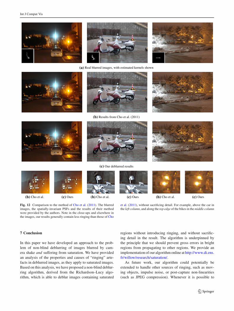
Figures 12 and 13 show the results of non-blind deblurringusing our algorithm, alongside those of the recently-proposedalgorithm of Cho et al. (2011). The blurred images and theirspatially-invariant PSFs are provided by Cho et al., alongwith their deblurred results2. In most cases our results exhibitless ringing than those of Cho et al. (2011), which is due tothe fact that we explicitly decouple the estimates of bright

2 http://cg.postech.ac.kr/research/deconv_outliers/ (accessed Novem-ber 12, 2011).

pixels from other pixels, in addition to removing saturatedblurred pixels.

In order to gauge the quantitative difference betweendeblurred images containing ringing and the results of ouralgorithm, we generated a set of synthetically blurred andsaturated images, with varying degrees of saturation andblur. We then deblurred using the original Richardson–Lucy algorithm, which produces ringing, and our proposedalgorithm. Figure 14 shows the results, indicating that ourmethod produces a measurable improvement in deblurredimage quality, which increases as the amount of saturationincreases.

123

Int J Comput Vis

(a)

(b)

(c)

(b) (c) (b) (c) (b) (c)

Fig. 12 Comparison to the method of Cho et al. (2011). The blurredimages, the spatially-invariant PSFs and the results of their methodwere provided by the authors. Note in the close-ups and elsewhere inthe images, our results generally contain less ringing than those of Cho

et al. (2011), without sacrificing detail. For example, above the car inthe left column, and along the top edge of the bikes in the middle column

7 Conclusion

In this paper we have developed an approach to the prob-lem of non-blind deblurring of images blurred by cam-era shake and suffering from saturation. We have providedan analysis of the properties and causes of “ringing” arte-facts in deblurred images, as they apply to saturated images.Based on this analysis, we have proposed a non-blind deblur-ring algorithm, derived from the Richardson–Lucy algo-rithm, which is able to deblur images containing saturated

regions without introducing ringing, and without sacrific-ing detail in the result. The algorithm is underpinned bythe principle that we should prevent gross errors in brightregions from propagating to other regions. We provide animplementation of our algorithm online at http://www.di.ens.fr/willow/research/saturation/.

As future work, our algorithm could potentially beextended to handle other sources of ringing, such as mov-ing objects, impulse noise, or post-capture non-linearities(such as JPEG compression). Whenever it is possible to

123

Int J Comput Vis

(a) (b) (c) (d) (e)

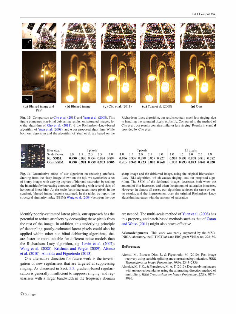
Fig. 13 Comparison to Cho et al. (2011) and Yuan et al. (2008). Thisfigure compares non-blind deblurring results, on saturated images, forc the algorithm of Cho et al. (2011), d the Richardson–Lucy-basedalgorithm of Yuan et al. (2008), and e our proposed algorithm. Whileboth our algorithm and the algorithm of Yuan et al. are based on the

Richardson–Lucy algorithm, our results contain much less ringing, dueto handling the saturated pixels explicitly. Compared to the method ofCho et al., our results contain similar or less ringing. Results in c and dprovided by Cho et al.

Fig. 14 Quantitative effect of our algorithm on reducing artefacts.Starting from the sharp image shown on the left, we synthesize a setof blurry images with varying degrees of blur and saturation by scalingthe intensities by increasing amounts, and blurring with several sizes ofhorizontal linear blur. As the scale factor increases, more pixels in thesynthetic blurred image become saturated. In the table, we report thestructural similarity index (SSIM) Wang et al. (2004) between the true

sharp image and the deblurred image, using the original Richardson–Lucy (RL) algorithm, which causes ringing, and our proposed algo-rithm. The SSIM of the deblurred images decreases both when theamount of blur increases, and when the amount of saturation increases.However, in almost all cases, our algorithm achieves the same or bet-ter results, and the improvement over the original Richardson–Lucyalgorithm increases with the amount of saturation

identify poorly-estimated latent pixels, our approach has thepotential to reduce artefacts by decoupling these pixels fromthe rest of the image. In addition, this underlying principleof decoupling poorly-estimated latent pixels could also beapplied within other non-blind deblurring algorithms, thatare faster or more suitable for different noise models thanthe Richardson–Lucy algorithm, e.g. Levin et al. (2007);Wang et al. (2008); Krishnan and Fergus (2009); Afonsoet al. (2010); Almeida and Figueiredo (2013).

One alternative direction for future work is the investi-gation of new regularisers that are targeted at suppressingringing. As discussed in Sect. 3.3, gradient-based regulari-sation is generally insufficient to suppress ringing, and reg-ularisers with a larger bandwidth in the frequency domain

are needed. The multi-scale method of Yuan et al. (2008) hasthis property, and patch-based methods such as that of Zoranand Weiss (2011) might also prove effective.

Acknowledgments This work was partly supported by the MSR-INRIA laboratory, the EIT ICT labs and ERC grant VisRec no. 228180.

References

Afonso, M., Bioucas-Dias, J., & Figueiredo, M. (2010). Fast imagerecovery using variable splitting and constrained optimization. IEEETransactions on Image Processing, 19(9), 2345–2356.

Almeida, M. S. C., & Figueiredo, M. A. T. (2013). Deconvolving imageswith unknown boundaries using the alternating direction method ofmultipliers. IEEE Transactions on Image Processing, 22(8), 3074–3086.

123

Int J Comput Vis

Bar, L., Sochen, N., & Kiryati, N. (2006). Image deblurring in the pres-ence of impulsive noise. International Journal of Computer Vision,70(3), 279–298.

Blake, A., & Zisserman, A. (1987). Visual Reconstruction. London:MIT Press.

Bouman, C., & Sauer, K. (1993). A generalized Gaussian image modelfor edge-preserving MAP estimation. IEEE Transactions on ImageProcessing, 2(3), 296–310.

Cai, J.-F., Ji, H., Liu, C., Shen, Z (2009). Blind motion deblurring froma single image using sparse approximation. In: Proc. CVPR

Chen, C., & Mangasarian, O. L. (1996). A class of smoothing functionsfor nonlinear and mixed complementarity problems. ComputationalOptimization and Applications, 5(2), 97–138.

Cho, S., & Lee, S. (2009). Fast motion deblurring. ACM Transactionson Graphics, 28(5), 145–148.

Cho, S., Wang, J., & Lee, S. (2011). Handling outliers in non-blindimage deconvolution. In:Proc ICCV

Chou, P. B., & Brown, C. M. (1990). The theory and practice of Bayesianimage labeling. International Journal of Computer Vision, 4(3), 185–210.

Fergus, R., Singh, B., Hertzmann, A., Roweis, S. T., & Freeman, W.T. (2006). Removing camera shake from a single photograph. ACMTransactions on Graphics, 25(3), 787–794.

Gamelin, T. W. (2001). Complex Analysis. New York: Springer-Verlag.Gupta, A., Joshi, N., Zitnick, C. L., Cohen, M., Curless, B. (2010).

Single image deblurring using motion density functions. In: Proc.ECCV

Harmeling, S., Hirsch, M., Schölkopf, B (2010a) Space-variant single-image blind deconvolution for removing camera shake. In:NIPS

Harmeling, S., Sra, S., Hirsch, M., Schölkopf, B (2010b) Multiframeblind deconvolution, super-resolution, and saturation correction viaincremental EM. In: Proc. ICIP.

Ji, H., & Wang, K. (2012). Robust image deblurring with an inaccurateblur kernel. IEEE Transactions on Image Processing, 21(4), 1624–1634.

Joshi, N., Kang, S. B., Zitnick, C. L., & Szeliski, R. (2010). Imagedeblurring using inertial measurement sensors. ACM Transactionson Graphics, 29(4), 30–39.

Krishnan, D., Fergus, R. (2009). Fast image deconvolution using hyper-Laplacian priors. In NIPS.

Krishnan, D., Tay, T., Fergus, R (2011). Blind deconvolution using anormalized sparsity measure. In: Proc. CVPR.

Levin, A., Fergus, R., Durand, F., & Freeman, W. T. (2007). Imageand depth from a conventional camera with a coded aperture. ACMTransactions on Graphics, 26(3), 70–79.

Levin, A., Weiss, Y., Durand, F., & Freeman, W. T. (2009). Understand-ing and evaluating blind deconvolution algorithms. MIT: Technicalreport.

Levin, A., Weiss, Y., Durand, F., & Freeman, W. T. (2011). Efficientmarginal likelihood optimization in blind deconvolution. CVPR: InProc.

Lucy, L. B. (1974). An iterative technique for the rectification ofobserved distributions. Astronomical Journal, 79(6), 745–754.

Richardson, W. H. (1972). Bayesian-based iterative method of imagerestoration. The Journal of the Optical Society of America, 62(1),55–59.

Schultz, R. R., & Stevenson, R. L. (1994). A bayesian approach toimage expansion for improved definition. IEEE Transactions onImage Processing, 3(3), 233–242.

Shan, Q., Jia, J., & Agarwala, A. (2008). High-quality motion deblur-ring from a single image. ACM Transactions on Graphics (Proc.SIGGRAPH 2008), 27(3), 73-1–73-10.

Tai, Y.-W., Du, H., Brown, M. S., & Lin, S. (2008). Image/video deblur-ring using a hybrid camera. CVPR: In Proc.

Tai, Y.-W., Tan, P., & Brown, M. S. (2011). Richardson-Lucy deblurringfor scenes under a projective motion path. IEEE PAMI, 33(8), 1603–1618.

Wang, Y., Yang, J., Yin, W., & Zhang, Y. (2008). A new alternating min-imization algorithm for total variation image reconstruction. SIAMJournal on Imaging Sciences, 1(3), 248–272.

Wang, Z., Bovik, A. C., Sheikh, H. R., & Simoncelli, E. P. (2004).Image quality assessment: From error visibility to structural similar-ity. IEEE Transactions on Image Processing, 13(4), 600–612.

Welk, M. (2010). Robust variational approaches to positivity-constrained image deconvolution. Technical Report 261, SaarlandUniversity, Saarbrücken, Germany.

Whyte, O. (2012). Removing camera shake blur and unwanted occlud-ers from photographs. PhD thesis, ENS Cachan.

Whyte, O., Sivic, J., Zisserman, A. (2011). Deblurring shaken and par-tially saturated images. In: Proc. CPCV, with ICCV.

Whyte, O., Sivic, J., Zisserman, A., Ponce, J. (2010). Non-uniformdeblurring for shaken images. In: Proc. CVPR.

Whyte, O., Sivic, J., Zisserman, A., & Ponce, J. (2012). Non-uniformdeblurring for shaken images. International Journal of ComputerVision, 98(2), 168–186.

Wiener, N. (1949). Extrapolation, interpolation, and smoothing of sta-tionary time series. London: MIT Press.

Xu, L., & Jia, J. (2010). Two-phase kernel estimation for robust motiondeblurring. In Proc. ECCV

Yang, J., Zhang, Y., & Yin, W. (2009). An efficient TVL1 algorithm fordeblurring multichannel images corrupted by impulsive noise. TheSIAM Journal on Scientific Computing, 31(4), 2842–2865. doi:10.1137/080732894.

Yuan, L., Sun, J., Quan, L., & Shum, H.-Y. (2007). Image deblurringwith blurred/noisy image pairs. ACM Transsactions on Graphics(Proc. SIGGRAPH 2007), 26(3), 1-1–1-10.

Yuan, L., Sun, J., Quan, L., & Shum, H.-Y. (2008). Progressive inter-scale and intra-scale non-blind image deconvolution. ACM Transac-tions on Graphics (Proc. SIGGRAPH 2008), 27(3), 74-1–74-10.

Zoran, D., & Weiss, Y. (2011). From learning models of natural imagepatches to whole image restoration. In Proc. ICCV

123