Passive processing of active nodal seismic data ... · 1 Passive processing of active nodal seismic data: Estimation of V P /V S - ratios to characteriz e structure and hydrology

1

Passive processing of active nodal seismic data: Estimation of VP/VS -

ratios to characterize structure and hydrology of an alpine valley infill Michael Behm1, Feng Cheng2, Anna Patterson1, Gerilyn Soreghan1

1School of Geology and Geophysics, University of Oklahoma, Norman, OK, United States 2Lawrence Berkeley National Laboratory, Berkeley, CA, United States 5

Correspondence to: Michael Behm ([email protected])

Abstract. The advent of cable-free nodal arrays for conventional seismic reflection and refraction experiments is changing the

acquisition style for active source surveys. Instead of triggering short recording windows for each shot, the nodes are

continuously recording over the entire acquisition period from the first to the last shot. The main benefit is a significant increase

in geometrical and logistical flexibility. As a by-product, a significant amount of continuous data might also be collected. 10

These data can be analysed with passive seismic methods and therefore offer the possibility to complement subsurface

characterization at marginal additional cost. We present data and results from a 2.4 km long active source profile which has

been recently acquired in Western Colorado (US) to characterize the structure and sedimentary infill of an over-deepened

alpine valley. We show how the ‘leftover’ passive data from the active source acquisition can be processed towards a shear

wave velocity model with seismic interferometry. The shear wave velocity model supports the structural interpretation of the 15

active P-wave data, and the P-to-S-wave velocity ratio provides new insights into the nature and hydrological properties of the

sedimentary infill. We discuss the benefits and limitations of our workflow and conclude with recommendations for acquisition

and processing of similar data sets.

1 Introduction

Seismic nodal acquisition systems (‘nodes’ thereafter) were introduced to the active source exploration community within the 20

last decade with the promise of geometrical flexibility and a more efficient production, especially in rugged terrain (Freed,

2008; Dean et al., 2013). Nowadays several outfitters provide instruments for a wide range of applications with a focus on the

energy industry (Dean et al., 2018), but nodal acquisition is also becoming widespread in the academic community (Karplus

and Schmandt, 2018). Nodes differ from conventional cable-based systems in several aspects. During recording, each node is

an autonomous data logger and recorder without required physical or non-physical connection to a central processing system. 25

They are designed to record continuously throughout the entire acquisition period, which might last from days to months. In

that regard, the acquired data can be considered as passive data which automatically include the shot windows from the active

sources. For any active seismic exploration study, the shot windows are considered as the complete data set to represent the

subsurface. In the case of continuous nodal acquisition, a significant amount of additional data is recorded outside the shot

windows. The lack of well-defined sources outside the active shooting times does not mean that these periods are seismically 30

quiet. The ambient noise spectrum covers a wide frequency range and stems from diverse natural and anthropogenic processes

Solid Earth Discuss., https://doi.org/10.5194/se-2019-47Manuscript under review for journal Solid EarthDiscussion started: 6 March 2019c© Author(s) 2019. CC BY 4.0 License.

2

(McNamara and Bulland, 2004; Riahi and Gerstoft, 2015). The location and timing of specific events within this noise spectrum

might be known with some degree of uncertainty (e.g. local, regional, and global seismicity), thus inviting classical active

processing methods like travel time tomography to derive local velocity models (Kissling, 1988; Byriol et al., 2013) or different

forms of receiver-side reflectivity mapping (Ruigrok et al., 2010; Behm and Shekar, 2014, Behm, 2018). For the more general

case of unknown locations and timing of the sources in the ambient noise spectrum (e.g. traffic noise, industrial activities) the 5

seismic interferometry method (Snieder, 2004; Wapenaar, 2004; Schuster, 2010) has become a staple for subsurface modelling

and interpretation. In particular, the extraction of surface waves travelling between receivers in locally deployed arrays can be

feasible for even relatively short time spans of ambient noise. (e.g. Nakata et al., 2011; Behm et al., 2014; Cheng et al. 2016).

The reconstructed surface waves are mostly used to image the local shear-wave velocity structure (e.g. Picozzi et al., 2009;

Hannemann et al., 2014) or for interpretation of temporal changes in the subsurface (e.g. Planes et al., 2015; Riahi et al., 2013). 10

Applied to active data, interferometric surface wave removal (Halliday et al., 2007, 2010) can successfully model and mitigate

unwanted Rayleigh-wave energy in shot gathers. Although body waves are much more challenging to extract from surface

recordings of ambient noise (Forghani and Snieder, 2010), the availability of many stations can facilitate signal processing

routines to focus on the extraction of diving waves (Nakata et al. 2015) and reflected waves (Draganov et al., 2009) as well.

Body waves caused by surface noise sources are also more likely to be detected in boreholes (Behm, 2017; Zhuo and Paulssen, 15

2017) or inside mines (Olivier et al., 2015).

Processing of passive data provides complementary information when compared to the active data. E.g. surface wave inversion

obtained from interferometry results in shear wave velocity models, and travel time tomography using local or regional

seismicity can increase the investigation depth. Strobbia et al. (2011) applied a workflow to isolate and invert Rayleigh waves

from a dense active source 3D acquisition, and in a later step used the obtained near-surface shear wave velocity model to 20

improve the filtering of Rayleigh wave energy for reflection processing. Most of the passive processing schemes provide

subsurface models with significantly lower lateral resolution than models obtained from active data. However, robust low-

resolution information can be beneficial when implemented into initial models for full waveform inversion (Sirgue and Pratt,

2004; Denes et al., 2009).

From a geologic point of view, our study focuses on the structure and sedimentary infill of an over-deepened alpine valley in 25

Western Colorado (US). Alpine valleys are of interest for geophysical investigation because of their significance for landform

evolution (e.g. incision rates, timing and effects of glacial overprinting; de Franco et al., 2009; Pomper et al., 2017) and their

potential for harbouring significant groundwater resources (e.g. Pugin et al., 2014). Brueckl et al. (2010) provide an overview

of geophysical exploration of glacially over-deepened valleys in the Austrian Alps of Europe. They report P-wave velocities

and densities for Quaternary sedimentary infill, and in all cases, they find a deeper sedimentary layer (“old valley fill”) above 30

the bedrock with higher P-wave velocities. Bleibinhaus and Hilberg (2012) investigate one of the largest over-deepened valleys

in the European Alps with seismic and electrical resistivity methods. Based on increased seismic velocities and decreased

resistivity, they interpret an aquifer in the shallow part of the sediments.


3

In our study, we present data and results from a local 2D reflection line acquired for imaging Unaweep Canyon on the

northeastern Colorado Plateau. Nodal instruments recorded continuously for the duration of 2.5 days and captured shots from

an active source as well as traffic-induced ambient noise. We apply seismic interferometry to the continuous data to extract

dispersive surface waves, which in turn are inverted for a 2D shear-wave velocity model of the valley structure. This model

complements the results from active source processing, and the joint interpretation of the active P-wave velocity and passive 5

S-wave velocity models allows for new insights on the nature and hydrologic properties of the sedimentary valley infill.

2 Area and Geology

The area of investigation (Fig. 1) is the western part of the NE-SW-trending Unaweep Canyon of the Uncompahgre Plateau,

western Colorado. This plateau is a large Cenozoic uplift on the northeastern Colorado Plateau and had a late Paleozoic

existence as the “Uncompahgre uplift” – one of several basement-cored uplifts with paired basins that formed as part of the 10

Ancestral Rocky Mountains (ARM) of western equatorial Pangaea (Kluth and Coney, 1981). Unaweep Canyon is an enigmatic

landform since the modern drainage divide occurs in the middle of the canyon, such that it hosts two creeks that drain to both

of its mouths. The canyon is deep (>400 m in inner Precambrian-hosted gorge), wide (locally >6000 m, 800 m in inner gorge),

and incised into Mesozoic strata and Precambrian crystalline basement. The canyon bottom hosts sedimentary fill of

Quaternary and possibly older age, at least 330 m thick in some regions (Soreghan et al., 2007). 15

Most suggest that the canyon was formed by the ancestral Gunnison River, and/or Colorado River in the late Cenozoic and

later abandoned (e.g., Cater 1966; Sinnock, 1981; Lohman, 1961; Hood, 2011; Aslan et al., 2014). Many attributes of the

canyon, however, are inconsistent with a purely fluvial origin, such as the lack of dendritic tributary systems, and apparent

glacial-like features such as U-shaped hanging valleys and truncated spurs (e.g. Cole and Young, 1983). However, Quaternary

glaciation did not extend down to the elevation of Unaweep Canyon, and glacial deposits are lacking (Soreghan et al., 2007). 20

An alternative hypothesis posits that the canyon was carved by glaciation in the late Paleozoic, and later exhumed by the

ancestral Gunnison River (Soreghan et al., 2007, 2008, 2014, 2015). A pre-Quaternary glacial origin remains controversial, in

part because the Uncompahgre uplift was equatorial during the late Paleozoic. Previous geophysical and drilling surveys

(Davogustto, 2006; Haffener, 2015) suggested that the valley might be over-deepened but were inconclusive regarding the

exact depths and the valley geometry. A recent approach focused on acquisition of high-resolution reflection seismic data in 25

fall 2017 (Patterson et al., 2018a, 2018b), and these data are also the basis for the present study.

3 Acquisition

The 2.4 km long reflection profile crosses the canyon in of its widest parts along a 4WD road, except for its first and last few

hundred meters (Fig. 2). Geophone installation, acquisition, and demobilisation was done within 2.5 days. Recording stations

were equipped with 385 Reftek ‘Texans’ data loggers / 4.5 Hz 1C geophones and with 120 Fairfield ZLand 3C 5 Hz nodes at 30


4

a 5 m interval. The ZLand nodes recorded continuously, while the Texans were only active during daytime due to memory

constraints. The shot spacing is 10 m in the northern part and 5 m in the southern part, where maximal over-deepening was

expected. Along the 4WD road, the truck-mounted and nitrogen-pressured A200 P&S source (Lawton et al., 2013) was utilized.

This source provided ample energy to record strong basement reflections from 400 – 600 m depth (Patterson et al. 2018a,

2018b; Fig. 3). Manual hammering with 18 lbs sledge hammer provided seismic energy off-road. For both the truck-mounted 5

source and the sledge hammer shots, five individual blasts were stacked at each shot location. All shot times were synchronized

to GPS time. Due to time constraints, the northern- and southernmost parts of the profile were shot simultaneously. Shooting

was done on Saturday and Sunday to avoid seismic noise from the a nearby active gravel pit. The state highway 141 intersects

the profile in the southern part. Traffic on this road was moderate (one car / truck every 1 to 5 minutes). All shot and receiver

locations were surveyed with high-precision RTK GPS. 10

The geometry of acquisition design was optimized for reflection processing, resulting in dense receiver and shot spacing. The

usage of nodal instruments was driven by logistical constraints, including partly steep and rough terrain, and a tight operational

schedule. Receiver deployment and shooting was essentially completed in two working days without prior scouting, which

would not have been possible with a conventional cable-based system and partly fresh untrained of student helpers. An

additional advantage of nodal acquisition is the possibility of recording at all offset ranges. Therefore, low-frequency 15

geophones were chosen deliberately to ensure registration of first arrivals at long offsets.

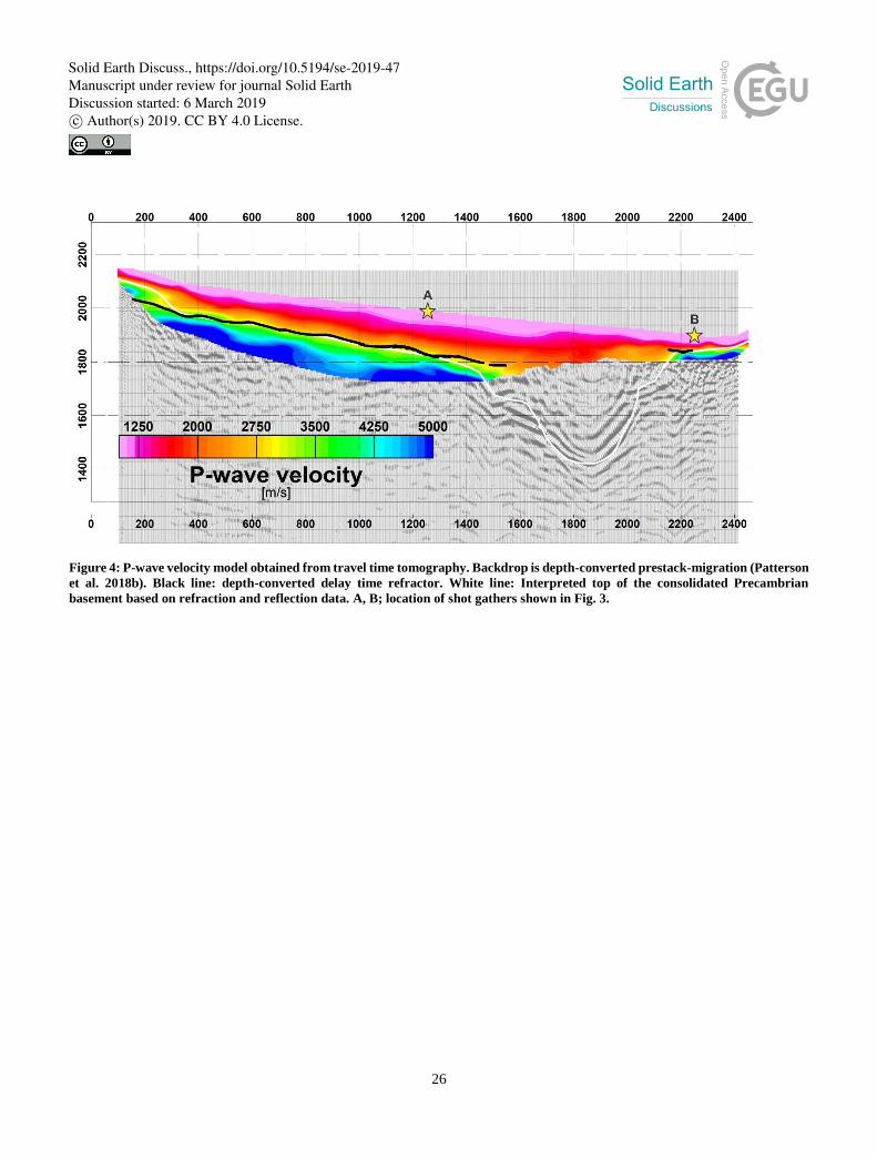
4 Active source data and processing

Reflection processing and interpretation is currently ongoing and initial results are presented by Patterson et al. (2018a) and

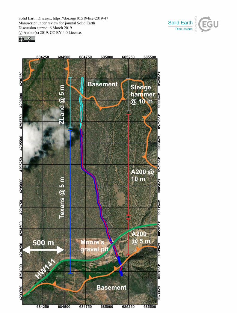
Patterson et al. (2018b). Here we focus on first arrival travel time tomography. In general, the first arrivals are of high S/N

(signal-to-noise) ratio, and they are visible up to 1.5 km offset (Fig. 3). The transition from low-velocity (1000 – 1500 m/s) 20

sediments to high-velocity (> 4000 m/s) basement is indicated at most parts of the profile by a distinct kink in the first arrival

travel time curve. This two-layer structure is not as clear towards the northern end of the profile, where the basement crops out

but still exhibits low velocities at short offsets. This is indicative of pronounced erosion and weathering effects. In the area of

expected over-deepening, refracted arrivals from the basement (Pb) are missing, while first arrivals through the sediments (Ps)

occur over longer offsets. 25

Overall, 18,263 sediment (Ps) and 16,104 basement travel time arrivals (Pb) are picked from the shot gathers. Signal processing

is limited to bandpass filtering (10-30-130-160 Hz) and Automated Gain Control (AGC). Travel time picks have been validated

by their reciprocal counterparts, wherever possible. Pb travel times represent refractions from the top of the consolidated

basement, and Ps travel times represent both sediments and weathered basement. Both Pb and Ps picks are integrated into one

combined first arrival time pick set. In case of overlap (<0.1% of all picks), the minimum of Pb and Ps is designated as the 30

first arrival.


5

3D first arrival travel time tomography is performed with the back-projection method of Hole (1992). Tests showed that a

simple depth-dependent initial velocity model leads to poor data fit and partly unrealistic velocities (> 7000 m/s) in the southern

part where the valley is expected to steepen. Therefore, we create a 2.5D initial velocity model from localized 1D inversions

of CMP-sorted travel times. Using this improved initial model, the 3D travel time inversion converges to the final model shown

in Fig. 4 after 9 iterations. Offset restrictions and smoothing filters are successively relaxed to build a detailed yet robust model 5

from top to bottom. The RMS travel time error of the final model is 0.03 s. The velocity model is indicative of over-deepening

in the southern part, where high basement velocities are missing. This is in accordance with the lack of Pb observations in the

shot gathers. Fig. 4 also includes a preliminary result of reflection imaging (depth-converted Kirchhoff Prestack time

migration; Patterson et al. 2018b) which allows unambiguous interpretation for over-deepening along profile distances 1600

m – 2000 m. 10

Interpretation of exact basement depths in smooth tomographic models is ambiguous due to inherent blurring of first-order

velocity discontinuities. Therefore, the Pb travel times are also subjected to a delay time decomposition approach (Telford et

al. 1990), providing the refractor structure in terms of delay times td and refractor velocities vR:

(1) 15

In equation (1), t(x) represents the picked Pb travel time at a specific offset x. vR is the refractor velocity and tdS / tdG are the

source and geophone delay times, respectively. Observing multiple shots at the same geophone locations leads to an

overdetermined linear equation system which is solved for vR, tdS, and tdG. The delay time equation system can be generalized

for laterally variable refractor geometry (Iwasaki, 2002). For a given vertical overburden velocity profile v(z), refractor depths 20

D and delay times td at a specific location are related by equation (2):

(2)

25

In equation (2), v(z) is taken from the first arrival tomography velocity field (Fig. 4) after capping velocities at 1800 m/s to

account for the blurring towards basement velocities. The obtained refractor depth coincides on average with the 2900 m/s -

isoline in the first arrival tomographic model at most parts of the profile, as well as with the strongest gradient in this velocity

field. The delay time solution is less reliable at the northern end of the profile where the assignment of Pb travel times is more

challenging due to a more variable refractor velocity. This is possibly caused by significant shallowing and outcropping of the 30

basement, which in turn leads to more stronger weathering effects, resulting in a more gradual velocity increase with depth.

𝑡(𝑥) =𝑥

𝑣𝑅

+ 𝑡𝑑𝑠 + 𝑡𝑑𝐺

𝑡𝑑 = ∫ √1

𝑣(𝑧)2−

1

𝑣𝑅2 𝑑𝑧

𝐷

0


6

At the southern end, Pb travel time assignment is also difficult due to the steep dip of the refractor. In the over-deepened

section, the lack of Pb travel times and large refractor dips prohibit delay time inversion. Refractor velocities range between

4300 m/s and 5600 m/s, with the lowest values in the center of the northern flat section. Considering the laterally varying

reliability and resolution of the three approaches (travel time tomography, delay time modelling, reflection imaging), we

manually build a combined interpretation of the consolidated basement (white line in Fig. 4). 5

5 Passive data and processing

The Texan data loggers recorded continuously during day time, and the ZLand nodes also recorded during night. Thus, a

significant amount of passive ambient noise data was acquired in addition to the active data. It is tempting to use interferometric

techniques (Wapenaar, 2010a; Schuster, 2010) to recover surface waves traveling between receivers from the ambient noise

field. Observed surface wave dispersion can be inverted for vertical variation of shear wave velocity structure. At local scales 10

with dense receiver spacing, most commonly phase velocity dispersion is obtained from Multi-Channel-Analysis (MASW;

Xia et al., 1999). Data recorded at larger and irregular receiver spacing is subjected to the Frequency-Time-Analysis (FTAN;

Bensen et al., 2007; Levshin et al., 1989; Hannemann et al., 2014) which provides group velocity dispersion.

The acquisition was performed during the seismically quiet weekend days to obtain high S/N ratio for the active data. Ambient

seismic noise interferometry requires noise sources in order to reconstruct the waves traveling between receiver stations. 15

Traffic on state highway 141 is moderate, but nonetheless contributes to the ambient noise spectrum. Two large 4WD trucks

were used for deployment and transporting the source, and their movements along the profile also generate surface wave

energy. Many other studies find traffic noise to be a dominant ambient noise source at local scales (Behm et al., 2014; Riahi

and Gerstoft, 2015; Chang et al., 2016), and specifically designed surveys are used for traffic noise imaging in urban areas

(Cheng et al., 2016). For our data set, active shooting during the day is also regarded as a major contributor to the ambient 20

seismic wave field.

A comparison of those different noise sources in the FK-domain is shown in Fig. 5. Ground roll can be discriminated from air

waves by its dispersive characteristics. Figs. 5a,d show the effect of a passing truck on highway 141, which excites Rayleigh

waves in the frequency range 1 – 15 Hz. Non-dispersive sound waves from a passing thunderstorm are clearly visible in Figs.

5b,e. This data subset also exhibits scattered ground roll with variable velocities and high frequencies. These scattered waves 25

are probably caused by the 4WD truck driving along the profile. Blasts from the truck-mounted source provide clear and

dispersive surface waves (Figs. 5c,f), but lack energy at the low end of the spectrum (< 2 Hz). Since the penetration depth of

surface waves is indirectly proportional to their frequency, the contribution of traffic noise potentially enables doubling of the

investigation depth of surface wave analysis. The 4.5 Hz 1C geophones appear to have a better response than the ZLand 5 Hz

3C stations. 30


7

5.1 Interferometry

Processing of the continuous data aims at deriving a 2D shear wave velocity model from the dispersive Rayleigh surface waves

which are obtained from interferometric processing. As most of the stations were equipped with 1C geophones (Texans), we

use the vertical component data only and extract Rayleigh waves. The workflow starts with cutting the continuous data into

30 seconds long time windows. Pre-processing is limited to temporal normalization (1-bit normalization; Bensen et al. 2007). 5

Spectral whitening is not applied since it is an intrinsic part of the following cross-coherence method used for the calculation

of the interferograms. Tests with substituting 1-bit normalization by Automated Gain Control (AGC) did not result in

significant changes in the interferograms. Interferogram calculation follows the virtual source method (Bakulin and Calvert,

2006), e.g. each 30 seconds long time window of each receiver station is cross-correlated with the corresponding time window

of all other stations. The cross-correlation GAB(f) between a receiver station B and a virtual source station A is calculated in 10

the spectral domain by equ. (3):

𝐺𝐴𝐵 (𝑓) =𝑋𝐵(𝑓)∙𝑋𝐴(𝑓)

‖𝑋𝐵(𝑓)‖∙‖𝑋𝐴(𝑓)‖+𝜀2 (3)

Equ. (3) is a measure of cross-coherence (Aki 1957; Prieto, Lawrence and Beroza 2009; Wapenaar et al. 2010b). In equ. (3), 15

XA(f) and XB(f) denote the Fourier transformation of the recorded and pre-processed data at stations A and B, respectively. The

overbar denotes complex conjugation. ε describes a stabilization term in case the product of the amplitude spectra approaches

zero, and it is chosen as 1% of the average amplitude spectra. The interferogram in the time domain is obtained from the

inverse Fourier transformation of GAB(f).

For each virtual source-receiver pair, the individual correlations of all 30 seconds long windows are stacked into one final 20

interferogram. Finally, 486 virtual source gathers are obtained (Fig. 6). The gathers show clear move-outs with varying

velocities in different frequency ranges, and with energy being distributed in the frequency range 2 – 15 Hz. The characteristics

of the causal and acausal parts indicate that the main source of the ambient noise is located towards the south, and traffic from

state highway 141 appears to be a significant contribution. Virtual source station 12040 (bottom panel in Fig. 6) is located

directly at the road, but still most of the stations southward exhibit dominant acausal surface waves, indicating noise sources 25

being located even further to the south. Besides road traffic and movements along the acquisition line, no other natural or

anthropogenic activity is expected to generate seismic noise in the observed frequency band in this widely unpopulated region.

We therefore propose that the steeply dipping mountain front in the south act as a reflector for surface waves generated at the

road and within the acquisition line, and backscatters all seismic energy towards the north. Observation of reflected low-

frequency earthquake surface waves are reported by Stich and Morelli (2007), and scattered and reflected surface waves are 30

common in exploration settings (Strobbia et al., 2011; Halliday et al., 2007, 2010). Behm et al. (2017) speculate on reflected

high-frequency surface waves as ambient noise sources from data acquired in a local network on an East Greenland glacier.


8

They also identify the steep basement cliffs as potential reflectors with providing and impedance contrast to the ice, and their

environmental settings (e.g., limited anthropogenic and natural sources) are similar to this study.

5.2 Inversion for S-wave velocity structure

The observed dispersion of surface waves in the virtual source gathers is inverted for the 2D shear-wave velocity structure 5

along the profile. We start with subdividing the profile into 25 100-m-long sections and perform source-receiver sorting of the

interferograms accordingly. All interferograms which have their virtual source and receiver station within one section are

assigned to this section. Within each section, all interferograms are stacked in 5 m – (absolute) offset bins, resulting in one

virtual shot gather representative of that section. By this approach, we take advantage of the multi-fold coverage while still

maintaining lateral resolution, and refrain from the effects of the topography on the surface wave propagation (Köhler et al., 10

2012; Ning et al., 2018). Subsequently, each stacked virtual shot gather is subjected to surface wave phase velocity dispersion

analysis, dispersion curve picking, and inversion for vertical shear wave velocity structure. This corresponds to the classical

MASW workflow (Multichannel Analysis of Surface Waves; Xia et al., 1999).

We employ the wavefield transformation method of Park et al. (1998) to image dispersion of the spectra of the surface waves.

We follow the energy peak to automatically pick the multimodal dispersion curves. Considering that the higher mode 15

dispersion curves only exist in a few sections, we pick the fundamental mode dispersion curves only. We further resample the

picked dispersion curve to ensure the efficiency of inversion as well as the coverage of multiple wavelengths. In this case, we

resample the lower frequency (< 8 Hz) part dispersion data along the wavelength axis with a 50 m sampling step, and the

higher frequency (> 8 Hz) part along the frequency axis with a 2 Hz sampling step.

The picked and resampled phase velocity dispersion curves are inverted for 1D shear wave velocity profiles VS(z) based on the 20

classical damped least-square method and singular-value decomposition technique (Xia et al., 1999). We use P-wave velocities

from the travel time tomography model (Fig. 4) and build the density model ρ(z) from the P-wave velocities VP(z) with

Gardner’s relation (Gardner et al., 1974):

𝜌(𝑧) = 0.31 ∙ 𝑉𝑃(𝑧)0.25 (4) 25

We set the maximum inversion depth to be half of the obtained maximum wavelength for each dispersion data. In general, this

method is fast and stable, and most inversions could be completed within 6~7 iterations with a minimum root-mean-squared

error at ~20 m/s. This error represents the misfit between the picked and prediced surface wave velocities.

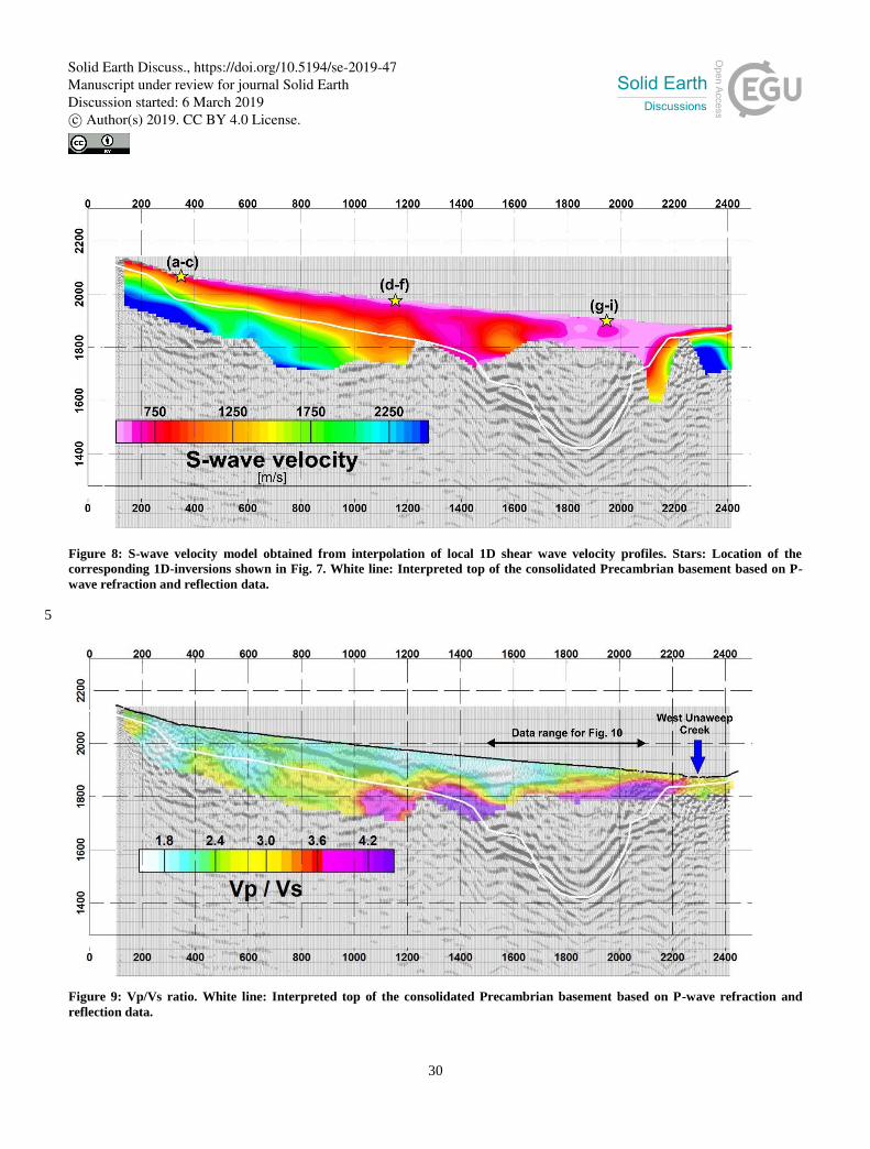
Fig. 7 presents examples of stacked virtual shot gathers (left panel), the measured and picked dispersion spectra (middle panel), 30

and the inverted VS(z) functions (right panel). The clear dispersion curves indicate a high S/N ratio of the stacked virtual shot

gathers. The virtual shot gathers refer to three locations (profile distances 350 m, 1150 m, 1950 m) as shown in Figure 8. The

dispersion spectra shows energy being distributed from 3 Hz to more than 35 Hz. We can also detect the air wave energy in


9

the dispersion spectra in Fig. 7b where the yellow line indicates a velocity of 340 m/s. The cyan curves indicate the final

dispersion curves used for inversion, where the error bar represents the width of the amplitude spectra which is used as a

weight in the inversion. The white dashed lines indicate the sampling power of the virtual shot gathers ranging from the

maximum to the minimum wavelength:

5

1

𝜆𝑚𝑖𝑛=

1

2∙𝑑𝑥 ,

1

𝜆𝑚𝑎𝑥=

1

𝐿 (5)

In equ. (5), dx and L refer to the geophone spacing (5 m) and the maximum offset (100 m), respectively. Therefore, the

maximum and minimum wavelengths calculate to 100 m and 10 m, and we set the upper limit of frequency range for the

picked dispersion curves to be ~35 Hz. According to the rule of thumb used in active surface wave survey, the minimum array 10

length should be 1.5 or 2 times of desired maximum wavelength (Xia et al., 2006; Foti et al., 2018). In our passive seismic

survey case, the whole profile is 2.4-km long, but each subdivided section is only 100-m-long. We suppose it is acceptable to

sample surface waves with ~250 m maximum wavelength for our profile, and the according lowest frequency of the dispersion

data used for inversion is about 3.5 Hz. Note that the dispersion signature at the location X=1950 m is different from the two

other ones and indicates a velocity inversion with depth (Shen et al., 2017). 15

The 25 VS(z) functions are assigned to the centre of their corresponding 100 m long sections and are interpolated along the

profile (Fig. 8). We observe the same large-scale structure as derived from the active source processing, e.g. thickening of the

low-velocity surface zone towards the south, lack of high velocities and decreased penetration depth in the over-deepened part,

and high velocities close to the surface at the southern end of the profile. A significant discrepancy is the apparent increase in

dip of the basement at the profile distance ~900 m when compared to the basement interpreted from active source data. 20

However, there is an indication of a basement velocity decrease in the tomographic P-wave velocity (Fig.4) model as well as

in the refactor velocity model, and basement reflections in the shot gathers suggest a sudden local change in dip at this location.

A buried basement fault or significantly fractured basement may explain this feature, but this is subject to further investigation.

The shallow S-wave velocity structure in the over-deepened section (profile distance ~1600 – 2100 m) is indicative of an

inversion zone (see also Figs. 7h,i) and is discussed in more detail in the next section. 25

6 Interpretation and Discussion

In geological settings, low seismic velocities are usually associated with poorly consolidated soils and rocks. This applies to

both P- and S-wave velocities, although S-wave velocities are more affected due to their sole dependence on the shear modulus.

The additional knowledge of the ratio of P- to S-wave velocities can help to further constrain subsurface properties. For

instance, a sudden increase of the P-to-S velocity ratio with depth is often used as an indicator for the groundwater table (GWT) 30

as shear-wave velocities experience no significant change when pore space voids are filled with fluid. In the oil & gas industry,


10

VP/VS – ratios are important in evaluating hydrocarbon saturation and lithology. Deep crustal studies rely on VP/ VS – ratios to

discriminate felsic from mafic rocks (Christensen, 1996; Carbonell et al., 2000; Morozov et al., 2001; Behm, 2009). On the

other end of the spatial scale, several VP/VS - studies for near-surface soils (< 50 m depth) exist as well. This is largely because

of the interest in shallow soil structure for geotechnical and hydrological applications and the ease at which shallow P- and S-

wave data can be acquired. Uyanik (2011) summarizes VP/VS – ratios of seismic measurements in shallow (< 20 m depth) 5

sediments (gravel, sand, clay-silt) with porosities ranging from 20% to 50%. He concludes that water saturation is indicated

by VP/ VS – ratios larger than 3.3 and reports maximum VP/VS – ratios for low-saturation (10% - 50%) soils of 5.0. Pasquet et

al. (2015) combine P-wave refraction, S-wave refraction, and surface wave inversion to image a shallow GWT (< 20 m depth)

in a weathered granitic basement. They state low VP/VS – ratios (<2.75) for the low-porosity/low-permeability granitic

basement and higher ratios (3.0 – 4.0) for wet soil close to the surface. 10

In-between the shallow surface and deep crustal / reservoir targets, only a small number of studies report VP/VS – ratios for

intermediate depths comparable to our study. Konstantaki et al. (2013) derive hydrological and soil mechanical parameters

across the Alpine Fault in New Zealand. They apply P-wave tomography and MASW to data from active shot gathers and

derive velocity models down to depths of 60 m. They find VP/VS – ratios larger than 3.0 and up to 9.0 for wet sand, gravel, and

silt lithologies, and were able to interpret the GWT from their results. Bailey et al. (2013) conducted a deep P- and S-wave 15

reflection survey in a geologic setting comparable to our study. Their site comprises a several hundred meters thick sedimentary

sequence of Quaternary sands and clays of Pleistocene age, which also includes lacustrine sediments. They were able to derive

VP/VS – ratios with high lateral and vertical resolution from the correlation of P- and S-wave reflections and from MASW. In

the shallow surface (< 50 m depth), they find VP/VS – ratios as high as 10, which were interpreted as soil pockets with high

potential for liquefaction. The deep structure (50 – 500 m depth) exhibits VP/VS – ratios between 3.0 and 6.0. Zuleta and Lawton 20

(2012) present a similar dataset comprising multicomponent data with P- and S-reflections. They investigate a late Paleozoic

sedimentary basin in British Columbia and derive VP/VS – ratios between 6.0 at the surface and 2.0 in depths of ca. 300 m.

Their velocities are comparable to our studies, e.g. VP is ranging from 1950 m/s to 2800 m/s, and VS is varying between 350

m/s and 1400 m/s.

We calculate the ratio of the tomographic P-wave velocity and the S-wave velocity models (Figs. 4, 8). In order to account for 25

the different parameterization of the travel time tomography and the dispersion inversion, we average P-wave velocities within

each surface wave inversion depth layer before we take the ratio. In the left part of the profile, we encounter VP/VS – ratios

between 1.8 and 2.5 for both the sedimentary cover and the basement. In combination with the actual velocities, these values

suggest dry conditions for the overburden. In case of the basement, VP/VS – ratios larger than 2 and moderate P-wave velocities

(4.0 – 5.5 km/s) are indicative of significant weathering of the Precambrian granites. The VP/VS – ratio changes to significantly 30

higher values (3.0 – 6.0) in the over-deepened part of the profile. The top of this zone of high VP/VS – ratios reaches the surface

at the southern part of the profile, where West Creek occupies the lowest topographic point. The zone dips towards the north

and its top is found at ca. 120 meters depth at the presumed northern edge of the over-deepened section. A northward dipping

reflector is found in a comparable depth range in the seismic image, and we therefore interpret the increased VP/VS – ratio in


11

the over-deepened section to represent the top of water-saturated sediments. Since the dip opposes the slope of the topography,

this aquifer needs to be confined or it is leaking through fractured basement in the north. The latter hypothesis would be

supported by the relatively low P- and S-wave velocities between profile distances 900 m to 1400 m (Figs. 4, 8).

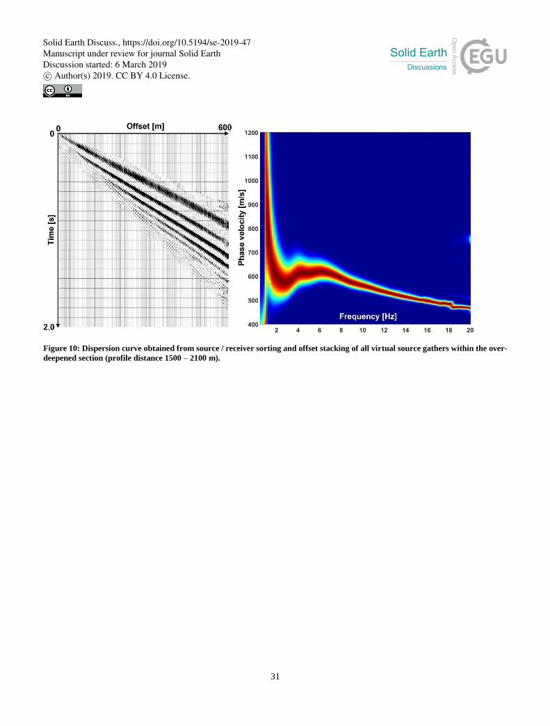
Both the tomographic P-wave velocity model and the S-wave velocity model from the stacked gathers with a maximum offset

range of 100 meters have only little penetration depth in the over-deepened section. To increase the investigation depth, we 5

extend the tomographic velocity model with interval velocities obtained from reflection processing (Patterson et. al., 2018b).

The two velocities models are tied together at an elevation of 1800 meters, where a smoothing filter is applied to account for

their different nature (smooth travel time tomography vs. discontinuous interval velocities). A deeper reaching S-wave velocity

model is derived from stacking all source-receiver sorted interferograms between the profile distances 1500 m and 2100 m.

The resulting maximum offset of 600 m allows for picking a dispersion curve with minimum frequencies around 1 Hz, which 10

in turn results in a significantly larger penetration depth of the inverted S-wave velocity model (Fig. 10). For both P- and S-

wave velocity models, the increase in investigation depth comes at the expense of reduced lateral resolution. However, at this

stage we are primarily interested in a representative 1D section of the over-deepened part. To calculate VP/VS, we again average

the P-wave velocities in the corresponding layer depths of the S-wave velocity model.

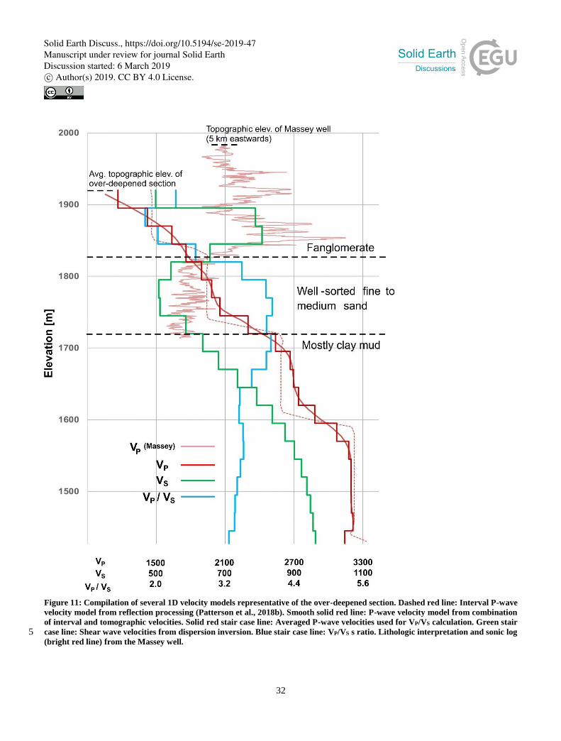
Fig. 11 shows a compilation of the 1D-velocity models in the over-deepened section. In general, the P-wave velocities in the 15

range 1200 – 2700 m/s correspond to those established for other Quaternary alpine valley fills (Brueckl et al., 2010; de Franco

et al., 2009). In Fig. 11, we also show the sonic log from the Massey well. This well is located upstream West Creek and 5 km

to the east of the seismic profile (Fig. 1), where the topographic elevation is also 80 m higher. The sonic log indicates a P-

wave velocity decrease at an elevation of ca. 1830 m, which correlates with a transition from Quaternary fanglomerates to

sand as seen in the core. The sand is interpreted to represent lacustrine sediments which were deposited 1.4 million years ago 20

when a landslide on the western side blocked the ancestral Gunnison River (Balco et al., 2013). Consequently, the top of the

lacustrine sediments should be found at the same elevation everywhere along West Unaweep canyon. The merged P-wave

velocity profile shows a discontinuity at this elevation, which however also indicates lower velocities above the sand. This

discrepancy might be explained by different heterogeneity and compaction of the Quaternary fanglomerate at the two locations.

Another possibility is a variable groundwater table, leading to saturated fanglomerates at the well location and dry fanglomerate 25

at the seismic profile. This is in fact supported by the VP/VS – ratio, which is low (2.0 – 2.5) above the top lacustrine horizon

and raises to significantly larger values (3.4 – 4.0) below. Bleibinhaus and Hilberg (2012) also report a similar P-wave velocity

increase for the transition from dry to saturated sand in Quaternary fill of the Salzach Valley in the European Alps. Lab analysis

of the core (pers. comm. O. Davugustto) provided an estimated porosity of 32% for the fanglomerate. This large value is

qualitatively supported by observation of the excavated material in the local gravel mining pit, which in generally is very 30

poorly sorted and comprises boulders with sizes up to a cubic meter and more. The increase in P-wave velocities correlates

with a decrease of S-wave velocities, which also suggests a vertical change of lithology. The base of the lacustrine sediments

is interpreted close to the bottom of the well, as the last few meters of the core transit into clayey mud. This transition also


12

correlates with a velocity discontinuity in the interval P-wave velocities and the onset of a gradual increase of the S-wave

velocities. Subsequently, the VP/VS – ratio below the sand is decreasing but still high (3.2 – 3.8).

Soreghan et al. (2007, 2008, 2014, 2015) speculate that the over-deepening of Unaweep Canyon was caused by glaciation in

a late Palaeozoic icehouse, and subsequently that the lacustrine sands lie on top of an upper Paleozoic sedimentary fill. The

prevailing upper Paleozoic strata in this region belong to the Cutler Formation (Werner, 1974; Soreghan et al., 2009). Exposed 5

Cutler Formation strata at the western mouth of Unaweep Canyon are indeed very poorly consolidated and poorly sorted

(Soreghan et al., 2007), and show signs of significant fluid alteration (Hullaster et al., 2019). Both observations qualitatively

agree with low seismic velocities and high VP/VS – ratio, although the effect of burial and subsequent compaction has not been

investigated yet. Overall, we interpret the high VP/VS – ratios as an indicator for significant saturation in the entire sedimentary

column below the fanglomerate. 10

Our interpretation is based on velocity models of different origins and of different parameterization. However, both the

tomographic P-wave model and the S-wave model from dispersion inversion do not explicitly comprise distinct velocity

discontinuities such as the prominent sediment-to-basement transition. Such an interface will be represented as a strong

gradient in an overall smooth velocity field, and the corresponding VP/VS will not allow for the exact definition of a groundwater 15

table. Nonetheless, the lateral variation of the VP/VS – ratio correlates with the seismic image and suggests the existence of an

aquifer in the over-deepened part (Fig. 9), an insight which could not be gained from P- or S-wave velocity models alone.

Surprisingly, the VP/VS does not give any indication for the transition from sediments to the basement in the northern part of

the profile, even though both P- and S-wave models sample the basement at sufficient depth ranges. This is indicative of

significant weathering of the top of the Precambrian granite. 20

The structural interpretation of the asymmetric valley structure and the steep and sudden dip at its southern rim is supported

by both the P-wave and S-wave velocity models (Figs. 4, 8). Dispersion analysis also gives better evidence of velocity inversion

zones than classical travel time tomography which is largely insensitive to velocity decrease with depth. However, in our case

the vertical trends of S- and P-wave velocities are partly decoupled due to water saturation.

The dense receiver spacing allows for relatively high lateral resolution of the S-wave velocity model through sorting and 25

stacking in source / receiver and offset bins, which comes at the expense of a loss in investigation depth. Nonetheless, even

with these short offsets the investigation depth is comparable to the P-wave travel time tomography using long offsets. This

compares to the results of Pasquet et al. (2015) who find larger penetration depths of surface wave inversion over S-wave

refraction. Improved S-wave velocity imaging and higher lateral resolution might be obtained from simultaneous inversion of

adjacent source / receiver cells (Konstantaki et al., 2013), or by calculating group velocity dispersion between individual 30

receiver pairs (Bensen et al., 2007; Hannemann et al, 2014). The latter approach would be applicable to irregular receiver

spacing but requires automatization of dispersion picking in case of a large number of receivers.

Sorting and stacking using larger offsets enables imaging of significantly larger depths, if low-frequency seismic energy is

present. In our case, the inclusion of traffic-induced ambient seismic noise provides frequencies as low as 1 Hz, which extends


13

the frequency spectrum of the active source (Fig. 5). Seismic interferometry and the virtual source method provide a very

efficient approach to merge the contributions from different active and passive seismic sources without the need for data

selection or tailored processing schemes.

7 Conclusions

We have combined active and passive processing schemes to derive P- and S-wave velocity models of an over-deepened alpine 5

valley. Both approaches complement each other in several aspects: (1) The P-wave velocity model is used to constrain the

shear wave velocity inversion; (2) Ambient noise sources extend the spectrum to lower frequencies, thus enabling the imaging

of deeper structures; (3) Independently derived P- and S-wave velocity models allow to calculate the VP/VS – ratio which adds

significantly to the geologic interpretation.

Our dataset shows that a deployment period as short as 30 hours in an area with little anthropogenic and natural seismic activity 10

still contains ample ambient noise. Much of this noise stems from acquisition down-time when the active source truck is

moving. Scattering and reflection of surface waves generate secondary sources which contribute to stationary phase sources

required for the application of ambient noise interferometry. Interferometry and the virtual source method naturally blend

active and ambient seismic sources without a need for separation of the two data domains.

Large-scale 3D seismic acquisition projects, as routinely performed in the energy sector or other industrial applications, involve 15

tens of thousands of active receivers, and those experiments might take weeks to months to be accomplished. If nodes are used,

then the sheer amount of passive data acquired with dense spatial sampling invite the application of processing workflows like

our study. Given the simplicity and high degree of automatization, detailed and robust subsurface models can be obtained

quickly and at marginal additional costs.

Equipping nodes with 3C sensors enables additional possibilities for processing of the acquired data. The observation of both 20

Rayleigh and Love waves increases the reliability of surface wave inversion. Well-established 3C methods from the global

seismology community (e.g. receiver functions, H/V ratio) can be adapted and downscaled to exploration applications.

To our knowledge, our study is the first one to report on the variation of VP/VS – ratios in sedimentary infills of alpine valleys.

The data suggest that Unaweep canyon hosts a significant aquifer as it is indicated by VP/VS – ratios larger than 3 over a vertical

extent of ca. 400 m. Since the resolution and accuracy of the seismic interpretation decreases with depth, a dedicated drilling 25

campaign would be beneficial to provide ground truth and calibrate the seismic models. Given the fact that quaternary

sedimentary strata cover a large range of the continental US (Soller and Garrity, 2018), our results invite the application of VP

and VS measurements in non-alpine regions as well. Many areas in the US mid-west are prone to droughts while at the same

time facing increased urbanization pressure, and influences by climate change. Mitigating these effects requires substantially

expanding our knowledge on the distribution and characterization of potential groundwater resources (Taylor et al. 2012). 30


14

Author contribution

M.Behm did the active and passive processing of the data and wrote the manuscript, except the parts noted below. F.Cheng

provided processing and description of the steps in section 5.2, and also contributed to processing of the active refraction data

data. A.Patterson processed the active reflection data and contributed to processing of the active refraction data. G.Soreghan 5

provided section 2 in the manuscript, and contributed to the interpretation

Competing interests

The authors declare that they have no conflict of interest.

10

Acknowledgements

Texan data loggers were provided by the IRIS PASSCAL instrument center. Acquisition was done in cooperation with the

Seismic Source Facility (SSF) based at University of Texas at El Paso. The dedication and competence of Galen Kaip and

Steve Harder contributed greatly to a successful acquisition. The Gateway community is thanked for local support. The project

is partially funded from NSF-EAR-1338331. The geologic map (Fig. 1) has been created by Eccles, T.M., Soreghan, G.S., 15

Kaplan, S.A., Patrick, K.D., and Sweet, D.E. Andy Elwood Madden, Kato Dee, and Jim Blattman are thanked for discussion

and helpful advice.

References

20

Aki, K.: Space and time spectra of stationary stochastic waves, with special reference to micro-tremors, Bulletin of the

Earthquake Research Institute 35, 415–457, 1957

Aslan, A., Hood, W.C., Karlstrom, K.E., Kirby, E., Granger, D.E., Kelly, S., Crow, R., Donahue, M.S., Polyak, V., and

Asmerson, Y.: Abandonment of Unaweep Canyon (1.4–0.8 Ma), western Colorado: Effects of stream capture and anomalously 25

rapid Pleistocene river incision: Geosphere, 10, 2014, doi:10.1130/GES00986.1.

Bailey, B. L., Miller, R.D., Peterie, S., Ivanov, J., Steeples, D., and Markiewicz, R.: Implications of Vp/Vs ratio on shallow

P and S reflection correlation and lithology discrimination, in: Expanded Abstracts of the 83rd Annual SEG Meeting,

Houston, USA, 22 – 27 September 2013, 1944-1949, 2013 30

Bakulin A., and Calvert, R: The virtual source method: Theory and case study, Geophysics 71, SI139–SI150, 2006


15

Balco G., Soreghan G.S., Sweet D.E., Marra K.R., and, Bierman P.R.: Cosmogenic-nuclide burial ages for Pleistocene

sedimentary fill in Unaweep Canyon, Colorado, USA, Quaternary Geochronology, 18, 149-157, 2013

Behm, M.: 3-D modelling of the crustal S -wave velocity structure from active source data: application to the Eastern Alps

and the Bohemian Massif, Geophys. J. Int., 179, 265–278, 2009 5

Behm, M., Leahy, G. M., and Snieder, R: Retrieval of local surface wave velocities from traffic noise - an example from the

La Barge basin (Wyoming), Geophys. Prospect., 62, 2014, doi:10.1111/1365-2478.12080, 2013

Behm, M., and Shekar, B.: Blind deconvolution of multichannel recordings by linearized inversion in the spectral domain. 10

Geophysics, 79, V33-V45, 2014

Behm, M.: Feasibility of borehole ambient noise interferometry for permanent reservoir monitoring, Geophysical Prospecting,

65, 563–580, 2017, doi:10.1111/1365-2478.12424

15

Behm, M., Walter, J.I., Binder, D., and Mertl, S.: Seismic Monitoring and Characterization of the 2012 Outburst Flood of the

Ice-Dammed Lake AP Olsen (NE Greenland), AGU Fall Meeting, New Orleans, USA, New Orleans, 11-15 December 2017,

C41D-1260, 2017

Behm, M.: Reflections from the Inner Core Recorded during a Regional Active Source Survey: Implications for the Feasibility 20

of Deep Earth Studies with Nodal Arrays, Seismological Research Letters, 89, 1698-1707, 2018, doi:10.1785/022018001

Bensen, G.D, Ritzwoller, M.H, Barmin, M.P., Levshin, A.L, Lin, F., Moschetti M.P., Shapiro, N. M., and Yang, Y.: Processing

seismic ambient noise data to obtain reliable broad-band surface wave dispersion measurements, Geophysical Journal

International, 169, 1239–1260, 2007 25

Biryol, C. B., Leahy, G.M., Zandt, G., and Beck, S.L.: Imaging the shallow crust with local and regional earthquake

tomography, Journal of Geophysical Research, 118, 2289–2306, 2013, doi: 10.1002/jgrb.50115. B

Bleibinhaus, F., and Hilberg, S: Shape and structure of the Salzach Valley, Austria, from seismic traveltime tomography and 30

full waveform inversion, Geophys. J. Int., 189, 1701–1716, 2012

Brückl, E., Brückl, J., Chwatal, W., and Ullrich, C.: Deep alpine valleys: Examples of geophysical explorations in Austria,

Swiss J. Geosci, 103, 329–344, 2010


16

Cater, F.W., Jr.: Age of the Uncompahgre Uplift and Unaweep Canyon, west-central Colorado: U.S. Geo- logical Survey

Professional Paper 550-C, C86–C92, 1966

Carbonell, R., Gallart, J., Perez-Estaun, A., Diaz, J., Kashubin, S., Mechie, J., Wenzel, F., and Knapp, J.: Seismic wide angle 5

constraints of the crust of the southern Urals, J. geophys. Res., 105, 13775–13777, 2000

Christensen, N.: Poisson’s ratio & crustal seismology, J. geophys. Res., 101, 3193–3156, 1996

Cole, R.D., and Young, R.G.: Evidence for glaciation in Unaweep Canyon, Mesa County, Colorado, in Averett, W.R., ed., 10

Northern Paradox Basin–Uncom- pahgre Uplift (Grand Junction Geological Society Field Trip Guidebook): Grand Junction,

Colorado, Grand Junction Geological Society, 73–80, 1983

Davogustto, O.E.: Soneo Gravimetrico en el Canon Unaweep: En Busca del Basamento y su Forma, B.S. Thesis, Simon Bolivar

University, Caracas, Venezuela, 56 pp, 2006 15

Dean, T., O’Connell, K., and Quigley, J.: A review of nodal land seismic acquisition systems, Preview, 164, 34-39, 2013, doi:

10.1071/PVv2013n164p34

Dean, T., Tulett, J., and Barnwell, R: Nodal land seismic acquisition: The next generation, First Break. 36, 47-52., 2018 20

Chang, J.P., de Ridder, S.Al.L, and Biondi, B.L.: High-frequency Rayleigh-wave tomography using traffic noise from Long

Beach, California, GEOPHYSICS, 81, B43-B53, 2016, doi.org/10.1190/geo2015-0415.1

Cheng, F., Xia, J., Luo, Y., Xu, Z., Wang, L., Shen, C., Lio, R., Pan, J., Mi, B, and Hu, Y.: Multi-channel analysis of passive 25

surface waves based on cross-correlations. Geophysics, 81(5), EN57-EN66, 2016, doi.org/10.1190/GEO2015-0505.1

Denes, V., Starr, E., and Kapoor, J.: Developing Earth models with full waveform inversion: The Leading Edge, 28, 432–435,

2009, doi: 10.1190/1 .3112760

30

Draganov, D., Campman, X., Thorbecke, J., Verdel, A., Wapenaar, K. Reflection images from ambient seismic noise,

Geophysics,74, A63–A67, 2009


17

Dou, S., Lindsey, N. J., Wagner, A., Daley, T. M., Freifeld, B. M., Robertson, M., Peterson, J., Ulrich, C., Martin, E.R., and

Ajo-Franklin, J. B: Distributed acoustic sensing for seismic monitoring of the near surface: A traffic-noise interferometry case

study. Scientific Reports, 7, 11620, 2017

Forghani, F., and Snieder, R.: Underestimation of body waves and feasibility of surface-wave reconstruction by seismic 5

interferometry, The Leading Edge, 29, 790–794, 2010, doi: 10.1190/1.3462779.

Foti, S., Hollender, F., Garofalo, F., Albarello, D., Asten, M., Bard, P.-Y., Comina, C., Cornou, C., Cox, B., Di Giulio, G.,

Forbriger, T., Hayashi, K., Lunedei, E., Martin, A., Mercerat, D., Ohrnberger, M., Poggi, V., Renalier, F., Sicilia, D., and

Socco, L.V.: Guidelines for the good practice of surface wave analysis: a product of the InterPACIFIC project, Bull. Earthq. 10

Eng., 16, 2367–2420, 2018

de Franco, R., Biella, G., Caielli, G., Berra, F., Guglielmin, M., Lozej, A., Piccin, A., and Sciunnach, D: Overview of high

resolution seismic prospecting in pre-Alpine and Alpine basins, Quat. Int., 204, 65–75, 2009

15

Freed, D.: Cable-free nodes: The next generation land seismic system, The Leading Edge, 27, 878-881, 2008

Gardner, G.H.F., Gardner, L.W., and Gregory, A.R.: Formation velocity and density - the diagnostic basics for stratigraphic

traps, Geophysics. 39, 770–780, 1974

20

Haffener, J.: Gravity modeling of Unaweep Canyon: Determining Fluvial or Glacial Origins: B.S. Thesis, University of

Oklahoma, Norman, Oklahoma, 25 pp, 2015

Halliday, D. F., Curtis, A., Robertsson, J. O., and van Manen, D.-J.: Interferometric surface-wave isolation and removal,

Geophysics, 72, A69–A73 2007 25

Halliday, D. F., Curtis, A.,Vermeer, P., Strobbia, C., Glushchenko, A., van Manen, D.-J, and Robertsson, J.O.A.:

Interferometric ground-roll removal : Attenuation of scattered surface waves in single-sensor data, Geophysics 75, SA15-

SA25, 2010

30

Hannemann, K., Papazachos, C., Ohrnberger, M., Savvaidis, A., Anthymidis, M., and Lontsi, A.M.: Three-dimensional

shallow structure from high-frequency ambient noise tomography: New results for the Mygdonia basin-Euroseistest area,

northern Greece, J. Geophys. Res, 119, 4979–4999, 2014


18

Hole, J.A.: Nonlinear high-resolution three-dimensional seismic travel time tomography, J. Geophys. Res., 97, 6553–6562,

1992

Hullaster D.P, Elwood-Madden, A.S., Soreghan, G.S., and Dee, K.T.: Redox interfaces of the proximal Permian Cutler

Formation, western Colorado: Implications for metal reactivity, American Chemical Society Annual Meeting, Orlando FL, 5

2019

Iwasaki, T.: Extended time-term method for identifying lateral structural variations from seismic refraction data, Earth Planets

Space, 54, 663–677, 2002

10

Karplus, M., and Schmandt, B.: Preface to the Focus Section on Geophone Array Seismology, Seismological Research

Letters,89, 1597, 2018

Kluth, C.F., and Coney, P.J.: Plate tectonics of the Ancestral Rocky Mountains, Geology, 9, 10–15, 1981, doi:10.1130/0091-

7613 15

Kissling, E.: Geotomography with local earthquake data, Reviews of Geophysics, 26, 65-698, 1988

Lawton, D.C., Gallant, E.V., Bertram, M.B., Hall, K.W., and Bertram, K.L.: A new S-wave seismic source, CREWES

Research Report, 25, 2013 20

Konstantaki, L.A., Carpentier., S., Garofalo, F., Bergamo, P., and Socco. L.V.: Determining hydrological and soil mechanical

parameters from multichannel surface-wave analysis across the Alpine Fault at Inchbonnie, New Zealand,

Near Surface Geophysics, 11, 435-448, 2013, doi:10.3997/1873-0604. 2013019

25

Levshin, A.L., Yanovskaya, T.B., Lander, A.V., Bukchin,B.G., Barmin, M.P., Ratnikova, L.I. & Its, E.N.: Seismic Surface

Waves in a Laterally Inhomogeneous Earth, ed. Keilis-Borok, V.I., Kluwer, Norwell, Mass., 1989

Lohman, S.W.: Abandonment of Unaweep Canyon, Mesa County, Colorado, by capture of the Colorado and Gunnison Rivers,

in Geological Survey Research 1961: U.S. Geological Survey Professional Paper 424, p. B144–B146, 1961 30

Maupin, V.: On the effect of topography on surface wave propagation in the ambient noise frequency range, J. Seismol., 221–

231, 2012


19

McNamara, D.E., and Buland, R.P.: Ambient Noise Levels in the Continental United States, Bulletin of the Seismological

Society of America, 94, 1517–1527, 2004 doi: https://doi.org/10.1785/012003001

Morozov, I., Smithson, S., Chen, J., and Hollister, L.: Generation of new continental crust and terrane accretion in Southeastern

Alaska and Western British Columbia: constraints from P- and S-wave wide-angle seismic data (ACCRETE), Tectonophysics, 5

341, 49–67, 2001

Nakata, N., Snieder, R., Tsuji, T., Larner, K., an, d Matsuoka, T: Shear- wave imaging from traffic noise using seismic

interferometry by cross- coherence, Geophysics, 76, SA97–SA106, 2011

10

Nakata, N., Chang, J. P., Lawrence, J. F. and Boué, P.: Body wave extraction and tomography at Long Beach, California, with

ambient-noise interferometry, J. Geophys. Res. Solid Earth, 120, 1159–1173, 2015, doi:10.1002/2015JB011870

Ning, L., Dai, T., Wang, L., Yuan, S., and Pang, J.: Numerical investigation of Rayleigh-wave propagation on canyon

topography using finite-difference method, J. Appl. Geophys., 159, 350–361, 2018 15

Olivier, G., Brenguier, F., Campillo, M., Lynch, R., and Roux, P.: Body-wave reconstruction from ambient seismic noise

correlations in an underground mine, Geophysics 80, KS11-KS25, 2015

Pasquet, S., Bodet, L., Longuevergne, L, Dhemaied, A., Camerlynck, C., Rejiba, F., and Guérin, R.: 2D characterization of 20

near-surface Vp/Vs: surface-wave dispersion inversion versus refraction tomography, Near Surface Geophysics, 13, 315-331,

2015, doi:10.3997/1873-0604.2015028

Patterson, A., Behm, M, and Soreghan, G.S.: Seismic investigation of Unaweep Canyon (Colorado): Implications for Late

Paleozoic alpine glaciation in the tropics, EGU General Assembly, Vienna, Austria, 8-13 April 2018, Geophysical Research 25

Abstracts, 20, EGU2018-8868, 2018a

Patterson, A., Chwatal, W., Behm, M, Cheng, F., and Soreghan, G.S: Seismic Imaging of and over-deepened alpine valley:

Implications for Late Paleozoic alpine glaciation of the Uncompahgre uplift (Western Colorado) , GSA Annual Meeting in

Indianapolis, Indiana, USA, 4-7 November 2018, Geological Society of America Abstracts with Programs, 50, 2018b, doi: 30

10.1130/abs/2018AM-319703

Picozzi, M., Parolai, S., Bindi, D., and Strollo, A.: Characterization of shallow geology by high-frequency seismic noise

tomography, Geophys. J. Int. 176, 164–174, 2009


20

Planes, T. et al.: Time-lapse monitoring of internal erosion in earthen dams and levees using ambient seismic noise.

Géotechnique, 2015, doi:10.1680/jgeot.14.P.268

Pomper, J. et al.: The glacially overdeepened trough of the Salzach Valley, Austria: Bedrock geometry and sedimentary fill of 5

a major Alpine subglacial basin, Geomorphology, 295, 147–158, 2017

Prieto, G., Lawrence, J.F, and Beroza, G.C: Anelastic Earth Structure from the Coherency of the Ambient Seismic Field,

Journal of Geophysical Research 114, B07303, 2009

10

Pugin, A. J. M., Oldenborger, G. A., Cummings, D. I., Russell, H. A. J., and Sharpe, D. R: Architecture of buried valleys in

glaciated Canadian Prairie regions based on high resolution geophysical data, Quat. Sci. Rev. 86, 13–23, 2014

Riahi, N., Bokelmann, G., Sala, P., and Saenger, E. H: Time-lapse analysis of ambient surface wave anisotropy: A three-

component array study above an underground gas storage, J. Geophys. Res., 118, 5339–5351, 2013 15

Riahi, N., and Gerstoft, P.: The seismic traffic footprint: Tracking trains, aircraft, and cars seismically, Geophys. Res. Lett.,

42, 2674–2681, 2015, doi:10.1002/2015GL063558.

Ruigrok, E., Campman, X., Draganov, D., and Wapenaar, K.: High- resolution lithospheric imaging with seismic 20

interferometry, Geophysical Journal International, 183, 339–357, 2010, doi: 10.1111/j.1365-246X.2010 .04724.x.

Schuster G.T. 2010. Seismic Interferometry. Cambridge University Press.

Shen C.: Dispersion characteristics and inversion of high-frequency surface waves in horizontal layered models with velocity 25

not increasing with depth (in chinese), Phd thesis, China university of Geosciences, 2017

Sinnock, S.: Pleistocene drainage changes in the Uncom- pahgre Plateau–Grand Valley region of western Colo- rado, including

formation and abandonment of Unaweep Canyon: A hypothesis, in Epis, R.C., and Callender, J.F., eds., Western Slope

Colorado: New Mexico Geological Society 32nd Field Conference Guidebook, 127–136, 1981 30

Sirgue, L., and Pratt, R.: Efficient waveform inversion and imaging: A strategy for selecting temporal frequencies, Geophysics,

69, 231–248, 2004, doi: 10.1190/1.1649391.


21

Snieder R.: Extracting the Green’s function from the correlation of coda waves: A derivation based on stationary phase. Phys.

Rev. E, 69, 046610, 2004

Soller, D.R., and Garrity, C.P.: Quaternary sediment thickness and bedrock topography of the glaciated United States east of

the Rocky Mountains, U.S. Geological Survey Scientific Investigations Map 3392, 2 sheets, scale 1:5,000,000, 2018, 5

doi.org/10.3133/sim3392.

Soreghan, G.S., Sweet, D., Marra, K., Eble, C., Soreghan, M., Elmore, R., Kaplan, S., and Blum, M.: An exhumed late

Paleozoic canyon in the Rocky Mountains, Journal of Geology, 115, 473–481, 2007, doi:10 .1086/518075.

10

Soreghan, G.S., Soreghan, M.J., Poulsen, C.J., Young, R.A., Eble, C.F., Sweet, D.E., and Davogustto, O.C.: Anomalous cold

in the Pangaean tropics, Geology, 36, 659–662, 2008

Soreghan G.S., Soreghan M.J., Sweet D. and Moore K.: Hot Fan or Cold Outwash? Hypothesized Proglacial Deposition in the

Upper Paleozoic Cutler Formation, Western Tropical Pangea., J Sediment Res 79, 495–522, 2009 15

Soreghan, G.S., Sweet, D.E., and Heavens, N.G.: Upland glaciation in tropical Pangaea: Geologic evidence and implications

for late Paleozoic climate modeling: Journal of Geology, 122, 137–163, 2014, doi:10 .1086/675255.

Soreghan, G. S., Sweet, D. E., Thomson, S. N., Kaplan, S. A., Marra, K. R., Balco, G., and Eccles, T. M: Geology of Unaweep 20

Canyon and its role in the drainage evolution of the northern Colorado Plateau, Geosphere, 2015,

http://doi.org/10.1130/GES01112.1

Strobbia, C., Laake, A., Vermeer, P., and Glushchenko, A.: Surface waves: use them then lose them. Surface-wave analysis,

inversion and attenuation in land reflection seismic surveying, Near Surface Geophysics, 9, 503-513, 2011 doi:10.3997/1873-25

0604.2011022

Taylor, R. et al.: Ground water and climate change, Nature Climate Change, 3, 322-329. 2012, doi:10.1038/nclimate1744

Telford, W.M., Geldart, L.P., and Sheriff, R.E.: Applied Geophysics, 2nd edn., Cambridge University Press, Cambridge, 1990 30

Uyanik, O.: The porosity of saturated shallow sediments from seismic compressional and shear wave velocities, Journal of

Applied Geophysics, 73, 16-24, 2011


22

Wapenaar K.: Retrieving the elastodynamic Green’s function of an arbitrary inhomogeneous medium by cross correlation,

Phys. Rev. Lett., 93, 254301, 2004

Wapenaar K., Draganov D., Snieder R., Campman X. and Verdel A.: Tutorial on seismic interferometry: Part 1 – Basic

principles and applications, Geophysics, 75, 75A195–75A209, 2010a 5

Wapenaar K., Slob E., Snieder R. and Curtis A: Tutorial on seismic interferometry: Part 2 – Underlying theory and advances.

Geophysics, 75, 75A211–75A227, 2010b

Werner W.: Petrology of the Cutler Formation (Pennsylvanian-Permian) near Gateway, Colorado, and Fisher Towers, Utah, 10

Journal of Sedimentary Research 44, 292–298., 1974

Xia, J., Miller, R. D. , and Park, C. B.: Estimation of near-surface shearwave velocity by inversion of Rayleigh wave:

Geophysics, 64, 691–700, 1999, doi: 10.1190/1.1444578.

15

Xia, J., Xu, Y., Chen, C., Kaufmann, R.D., and Luo, Y.: Simple equations guide high-frequency surface-wave investigation

techniques, Soil Dyn. Earthq. Eng., 26, 395–403, 2006

Zhou, W., and Paulssen, H: P and S velocity structure in the Groningen gas reservoir from noise interferometry.

Geophysical Research Letters, 44, 11,785–11,791, 2017, doi.org/10.1002/2017GL075592 20

Zuleta, L.M., and Lawton, D.C.: Vp/Vs characterization of a shale gas basin, northeast British Columbia, Canada, in: Expanded

Abstracts of the 82nd Annual SEG Meeting, XXX, Las Vegas, 4 – 9 November 2012, 1944-1949, 2012,

doi.org/10.1190/segam2012-1172.1

25

30

Figures


23

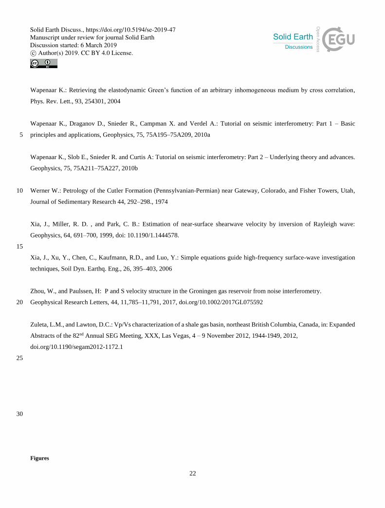
Figure 1: Surface geology of Western Unaweep Canyon and location of geophysical transects. pC: Precambrian granites (basement);

Qu: Unconsolidated Quaternary deposits; Qt: Talus deposits; TRC, TRW, Je, Jk: Mesozoic sediments; Red line: Seismic acquisition 5 2017 (this study); Blue line: Seismic acquisition 2005; Green lines: Gravimetric acquisition 2006, 2014. Massey #1, #2: Wells (TVD

320 m).


24


25

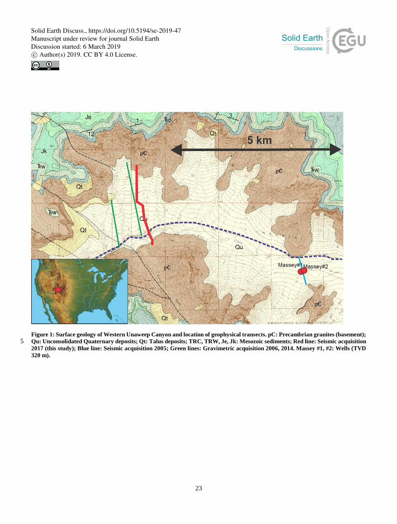
Figure 2: Geometry of the 2017 seismic acquisition. Thick blue line: Texan 1C receivers; Thick cyan line: Fairfield 3C nodes; Red

triangles: Shot locations of the A200 P&S source; Grey triangles: Shot locations of the sledge hammer; Green line: Road 141.

Figure 3: Seismic data examples: Shot gathers A, B (location see Fig. 4) filtered in different frequency bands. Pb: refractions from 5 the basement; Ps: refractions from the overburden (sediments); PbP: basement reflections; R; Rayleigh waves from the active

source, but not also traffic-induced ground roll.


26

Figure 4: P-wave velocity model obtained from travel time tomography. Backdrop is depth-converted prestack-migration (Patterson

et al. 2018b). Black line: depth-converted delay time refractor. White line: Interpreted top of the consolidated Precambrian

basement based on refraction and reflection data. A, B; location of shot gathers shown in Fig. 3.


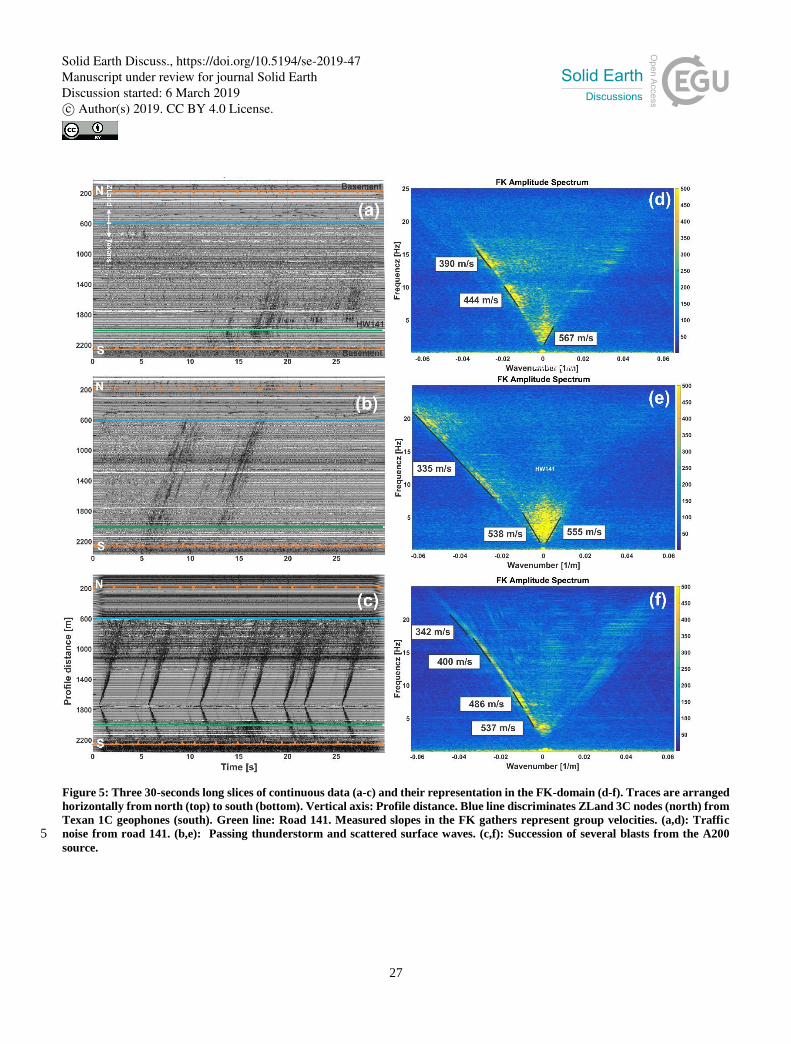
27

Figure 5: Three 30-seconds long slices of continuous data (a-c) and their representation in the FK-domain (d-f). Traces are arranged

horizontally from north (top) to south (bottom). Vertical axis: Profile distance. Blue line discriminates ZLand 3C nodes (north) from

Texan 1C geophones (south). Green line: Road 141. Measured slopes in the FK gathers represent group velocities. (a,d): Traffic

noise from road 141. (b,e): Passing thunderstorm and scattered surface waves. (c,f): Succession of several blasts from the A200 5 source.


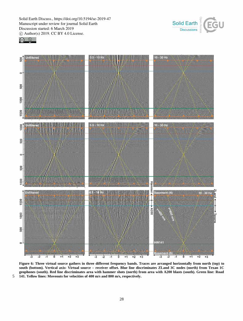
28

Figure 6: Three virtual source gathers in three different frequency bands. Traces are arranged horizontally from north (top) to

south (bottom). Vertical axis: Virtual source – receiver offset. Blue line discriminates ZLand 3C nodes (north) from Texan 1C

geophones (south). Red line discriminates area with hammer shots (north) from area with A200 blasts (south). Green line: Road

141. Yellow lines: Moveouts for velocities of 400 m/s and 800 m/s, respectively. 5


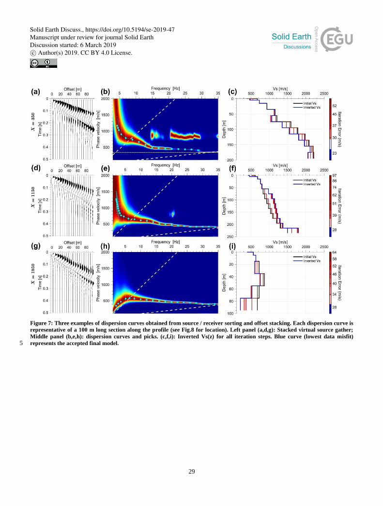
29

Figure 7: Three examples of dispersion curves obtained from source / receiver sorting and offset stacking. Each dispersion curve is

representative of a 100 m long section along the profile (see Fig.8 for location). Left panel (a,d,g): Stacked virtual source gather;

Middle panel (b,e,h): dispersion curves and picks. (c,f,i): Inverted Vs(z) for all iteration steps. Blue curve (lowest data misfit)

represents the accepted final model. 5


30

Figure 8: S-wave velocity model obtained from interpolation of local 1D shear wave velocity profiles. Stars: Location of the

corresponding 1D-inversions shown in Fig. 7. White line: Interpreted top of the consolidated Precambrian basement based on P-

wave refraction and reflection data.

5

Figure 9: Vp/Vs ratio. White line: Interpreted top of the consolidated Precambrian basement based on P-wave refraction and

reflection data.


31

Figure 10: Dispersion curve obtained from source / receiver sorting and offset stacking of all virtual source gathers within the over-

deepened section (profile distance 1500 – 2100 m).


32

Figure 11: Compilation of several 1D velocity models representative of the over-deepened section. Dashed red line: Interval P-wave

velocity model from reflection processing (Patterson et al., 2018b). Smooth solid red line: P-wave velocity model from combination

of interval and tomographic velocities. Solid red stair case line: Averaged P-wave velocities used for VP/VS calculation. Green stair

case line: Shear wave velocities from dispersion inversion. Blue stair case line: VP/VS s ratio. Lithologic interpretation and sonic log 5 (bright red line) from the Massey well.


Documents

Passive processing of active nodal seismic data ... · 1 Passive processing of active nodal seismic data: Estimation of V P /V S - ratios to characteriz e structure and hydrology