Embed Size (px)
Citation preview
Passenger Demand for Air Transportation in a Hub-and-Spoke Network
by
Chieh-Yu Hsiao
B.B.A. (National Chiao Tung University, Taiwan) 1994
M.S. (National Chiao Tung University, Taiwan) 1996
A dissertation submitted in partial satisfaction of the
requirements for the degree of
Doctor of Philosophy
in
Engineering-Civil and Environmental Engineering
in the
Graduate Division
of the
University of California, Berkeley
Committee in charge:
Professor Mark M. Hansen, Chair
Professor Samer M. Madanat
Professor Bronwyn H. Hall
Fall 2008

The dissertation of Chieh-Yu Hsiao is approved:
------"----'-"-'-------r--- Date (~/2 ~/of'
_----c~~~~~~----Date Jo/J4!CJ 3
--+-$--=-~===--';'~----I-f-~~-- Date Je)JL~/0 ()
University of California, Berkeley
Fall 2008
Passenger Demand for Air Transportation in a Hub-and-Spoke Network
Copyright 2008
by
Chieh-Yu Hsiao
1
Abstract
Passenger Demand for Air Transportation in a Hub-and-Spoke Network
by
Chieh-Yu Hsiao
Doctor of Philosophy in Engineering-Civil and Environmental Engineering
University of California, Berkeley
Professor Mark M. Hansen, Chair
A major transformation of the air transportation system—involving the
modernization of technologies, policies, and business models—is currently under way.
Knowledge of passenger demand for air service is the key to a successful system
transformation. This research develops an air passenger demand model and applies it to
the air transportation system of the United States.
The proposed model deals with city-pair demand generation and demand
assignment (to routes) in a single model, which is consistent with random utility theory. It
also quantifies the “induced” air travel by adding a non-air alternative in the choice set.
Using publicly available and regularly collected panel data, the model captures both time
series and cross-sectional variation of air travel demand, and can be regularly updated.
The empirical analysis explicitly modeled the pattern of correlations among alternatives
by a three-level nested logit model. This implies that a route is more likely to compete
with another route of the same O-D airport pair in a multiple airport system than the
routes of the other 0-0 airport pairs, and is least likely to be substituted by the non-air
alternative. In addition, the endogeneity problem of air fare was identified and remedied
by the instrumental variables (IV) method. The IV estimates yield more sensible
values-of-time, demand elasticities, and correlations of total utilities for alternatives than
those of ordinary least squares method.
Other empirical findings include that (1) the fare elasticities from our estimates
accord with the variation of fare elasticities from other studies in the literature; (2) for
connecting routes, a proportional flight frequency increase on the segment with lower
frequency increases service attractiveness more than an equivalent change on higher
frequency segment; (3) travelers avoid connecting at airports with high expected delay;
(4) under steady state, a one-minute hub delay increase has a larger impact on demand
than an equivalent change in scheduled flight time of a connecting route; (5) air travel
demand is strongly sensitive to income; (6) market distance has a concave effect on air
route demand; and (7) potential travelers' fare sensitivity has increased relative to
frequency sensitivity since 2001.
Professor Mark M. Hansen
Dissertation Committee Chair
2
i
Table of Contents
Chapter 1 Introduction ........................................................................................................ 1
Chapter 2 A Passenger Demand Model for Air Transportation ......................................... 8
2.1 Literature Review .................................................................................................. 8
2.1.1 Overview ..................................................................................................... 8
2.1.2 Demand Generation Model ....................................................................... 10
2.1.3 Demand Assignment Model ...................................................................... 12
2.1.4 Discussion and Summary .......................................................................... 17
2.2 The Demand Model ............................................................................................. 25
2.2.1 Conceptual Framework ............................................................................. 25
2.2.2 Saturated Demand Function ...................................................................... 29
2.2.3 Market Share Function .............................................................................. 31
Chapter 3 Empirical Analysis of the Passenger Demand for Air Transportation ............. 39
3.1 Model Specifications ........................................................................................... 39
3.1.1 Model Forms and Nesting Structures ........................................................ 39
3.1.2 Causal Factors ........................................................................................... 56
ii
3.2 Data ...................................................................................................................... 75
3.3 Model Estimation ................................................................................................. 85
3.4 Estimation Results ............................................................................................... 88
Chapter 4 Implications and Applications ........................................................................ 106
4.1 Demand Elasticities ........................................................................................... 106
4.1.1 Demand Elasticity with respect to Fare ................................................... 107
4.1.2 Demand Elasticity with respect to other Variables ................................. 114
4.2 Policy Experiments ............................................................................................ 120
4.2.1 Fare Experiment ...................................................................................... 121
4.2.2 Delay Experiments .................................................................................. 124
4.2.3 Summary and Discussions of Policy Experiments .................................. 128
4.3 Structural Changes over Time ........................................................................... 130
4.3.1 Estimation Results and Discussion .......................................................... 131
4.3.2 Sensitivities to Fare and Frequency ......................................................... 139
Chapter 5 Conclusions and Recommendations ............................................................... 144
5.1 Conclusions ........................................................................................................ 144
iii
5.1.1 Methodological Contributions ................................................................. 144
5.1.2 Empirical Findings .................................................................................. 146
5.2 Recommendations .............................................................................................. 153
References ....................................................................................................................... 158
Appendix A The Saturated Demand ............................................................................... 167
Appendix B Derivation of Estimation Equations ........................................................... 170
iv
List of Figures
Figure 2.1 Categorizations of Models ................................................................................. 9
Figure 2.2 City-Pair Air Passenger Demand in a Hub-and-Spoke Network .................... 26
Figure 3.1 Nesting Structure: Multinomial Logit ............................................................. 40
Figure 3.2 Nesting Structure: Two-Level Nested Logit ................................................... 43
Figure 3.3 Nesting Structure: Three-Level Nested Logit—A .......................................... 46
Figure 3.4 Nesting Structure: Three-Level Nested Logit—B ........................................... 49
Figure 3.5 Nesting Structure: Four-Level Nested Logit ................................................... 53
Figure 3.6 Decomposition of Total Travel Time (except for Ground Access Time) ....... 62
Figure 3.7 Delay and Utility ............................................................................................. 69
Figure 3.8 Components of Market Distance Effect .......................................................... 73
Figure 3.9 Cumulative Passenger Shares of Airports ....................................................... 79
Figure 3.10 Market Distance Effects .............................................................................. 100
Figure 4.1 Market Demand Elasticities with Respect to Fare ........................................ 110
Figure 4.2 Route Demand Elasticities with Respect to Fare (IV Estimates) .................. 112
Figure 4.3 Markets (Passengers) with Negative Distance Elasticities ............................ 117
v
Figure 4.4 Results of Fare Experiments .......................................................................... 122
Figure 4.5 Results of System Delay Experiments .......................................................... 125
Figure 4.6 Results of ORD Delay Experiments .............................................................. 127
Figure 4.7 Delay Effects on Air Route Demand ............................................................. 138
Figure 4.8 Coefficient Ratios of Fare to Frequency ....................................................... 140
Figure 4.9 Medians of Route Demand Elasticities ......................................................... 142
vi
List of Tables
Table 2.1 Features of Different Models ............................................................................ 24
Table 3.1 On-Time Performance Metrics of a Route ....................................................... 67
Table 3.2 Multiple Airport Systems.................................................................................. 82
Table 3.3 Summary Statistics ........................................................................................... 84
Table 3.4 Panel Data Estimation Results of Level 3 ........................................................ 90
Table 3.5 Inferred Values of Travel Time ........................................................................ 92
Table 3.6 Panel Data Estimation Results of Level 2 ........................................................ 96
Table 3.7 Panel Data Estimation Results of Level 1 ........................................................ 98
Table 3.8 Summary and Comparisons of Panel Data Estimation Results ...................... 102
Table 3.9 Sensitivity Tests for Saturated Demand Settings ............................................ 105
Table 4.1 Demand Elasticities with Respect to Fare ...................................................... 108
Table 4.2 Market Demand Elasticities ............................................................................ 115
Table 4.3 Route Demand Elasticities .............................................................................. 119
Table 4.4 Annual Data Estimation Results—NL3B-OLS Estimates .............................. 133
Table 4.4 Annual Data Estimation Results—NL3B-OLS Estimates (Continued) ......... 134

vii
Table 4.5 Annual Data Estimation Results—NL3B-IV Estimates ................................. 135
Table 4.5 Annual Data Estimation Results—NL3B-IV Estimates (Continued) ............. 136

viii
Acknowledgements
I would like to express my gratitude to many people and organizations for their
contributions to this dissertation and my study at Berkeley.
Professor Mark Hansen, my advisor, guided me through every stage of this
dissertation. His critical suggestions and proofreading significantly improved this work.
Without his humor, encouragement and financial support, this research would not have
been completed.
I would like to thank Professor Samer Madanat and Professor Bronwyn Hall for
serving as my dissertation committee members. Professor Hall could have enjoyed her
semi-retirement and relaxed; instead she carefully read through drafts of this dissertation
and provided valuable suggestions. For this, I am extremely grateful. Moreover, the
instrumental variable used in this research was inspired by her great lectures and by
discussions with her.
My memorable experience of studying at Berkeley was enriched with professors
and fellow students. I gained a lot from excellent lectures given by Professors Mark
Hansen, Adib Kanafini, Carlos Doganzo, Martin Wachs, Samer Madanat, Michael
Cassidy, Bronwyn Hall, Matthew Rabin, Kenneth Chay, and Shmuel Oren. Lunching and
discussing with fellow students, especially Lyle Tripp, Pei-Chen Liu, Peng-Chu Chen,
Avijit Mukherjee, Tatjana Bolic, and Wanjira Jirajaruporn were unforgettable and
fruitful.

ix
My life in the US would have been much worse without the friendship with the
Tripp and Lu families. I am grateful that Hazel and Lyle Tripp, who helped to decide my
children’s English names, have been proposing good places for visits and food, and been
so nice to my children. May and Leo Lu have been treating my children like theirs, and
we enjoyed numerous great weekends together.
I would express my deepest gratitude towards my family members, whose love is
indispensable for my overseas study. The full support from my parents gave me the
greatest flexibility in my professional carrier. My sisters (and their families) shared my
family commitments when I was physically absent from hometown for many years. My
wife spent most of her time with me and our lovely children, Grant and Sophie. This
allowed me to concentrate on my dissertation and have much fun with Grant and Sophie
in my spare time.
I would also like to acknowledge additional financial support from the Ministry of
Education, Taiwan (under the government scholarship to study abroad), and the National
Science Council, Taiwan (under the Taiwan Merit Scholarships TMS-094-1-A- 060).
1
Chapter 1 Introduction
A major transformation of the air transportation system—involving the
modernization of technologies, policies, and business models—is currently under way.
Knowledge of passenger demand for air service is the key to a successful system
transformation. For instance, in the United States, the Next Generation Air Transportation
System (NextGen)1 programs endeavor, in part, to expand capacity and accommodate
future traffic growth. While overestimating future traffic leads to overinvestment,
underestimating future traffic distorts system operations and causes poor system
performance, thereby increasing user (e.g. airlines and travelers) costs. A better
understanding of passenger demand will make the expansion more cost-beneficial.
Current understanding2 of the demand for air service fails to address several
significant questions: (1) What is the relative importance of causal factors (such as cost,
flight frequency, directness of routing, on-time performance, and income) in determining
demand and demand assignment among routes? (2) How have these relationships
changed over time? (3) What is the appropriate structure for nesting the wide array of
route alternatives, which encompass alternate terminal airports, routing types, connecting
hubs, as well as the possibility of not traveling (by air ) at all?
1 According to Joint Planning and Development Office (2007), “the goal of NextGen is
to significantly increase the safety, security, capacity, efficiency, and environmental compatibility of air transportation operations, and by doing so, to improve the overall economic well-being of the country.” Refer to Joint Planning and Development Office (2004; 2007) for more information.
2 Details are discussed in the section of literature review (section 2.1).
2
Appropriately identifying causal factors and quantifying their effects contribute to
the fundamental understanding of air travel demand and allow sensible predictions of
demand response to a wide range of future scenarios, including different levels of
congestion, network connectivity, aircraft size and frequency, and fuel price, among other
factors. Existing models are not sufficient to meet these purposes for several reasons, as
discussed below.
Most existing models in the literature only deal with either demand generation or
demand assignment, or treat these two phenomena sequentially. The sequential approach
is inappropriate since it implicitly assumes that the total demand volume is independent
of alternative cost and service quality. In addition, studies in air demand literature usually
include cost and flight frequency as causal factors, other factors—such as on-time
performance—are seldom investigated. Specifying these additional causal factors not
only allows predictions of demand response to changes in these factors, but also affects
the estimated effects of cost and flight frequency. More importantly, although most
studies in air demand literature recognize the importance of fare in air demand, few of
them deal with the endogeneity problem of fare, which may bias the estimated effects of
all causal factors.
Changes in the structure of air travel demand over time are of interest and seldom
studied. Possible reasons for the structural include changing distribution channels and the
entry of low-cost carriers. Rapid development of the Internet and its use to purchase air
travel may affect the structure of airline service demand by increasing the availability of
travel information and reducing the role of travel agents. Entry of low cost carriers may
3
increase expectations for lower fares and the tendency of consumers to search for them.
Examining trends in the structure of air travel demand can reveal whether and to what
extent such changes have occurred, and thereby reveal the prospects for similar dynamics
in the future.
Air travelers and potential air travelers face a rich array of travel alternatives, from
whether to travel, to what airports to fly between, to their routing, airline, flight, and
service class. Some alternatives are very similar to each other while others are quite
different. In the formulism of random utility theory upon which this research is based
similarity between alternatives is captured by the correlations between their stochastic
utilities: if an individual that is predisposed toward alternative A is also likely to be
predisposed toward alternative B, we consider A and B to be correlated. We seek to
understand the pattern of such correlation evidenced in the distribution of traffic among
routes (including the “null route” of not traveling by air). Such patterns are of inherent
interest, and must be properly represented in order to accurately estimate effects of causal
factors, and are critical in predicting how demand will respond to changes in service
supply.
In sum, existing air travel demand models and literature have several shortcomings
that this research seeks to address. In so doing we contribute to both fundamental
understanding of air travel demand and the practical need to predict how demand will
respond to a range of future scenarios. Specific objectives and an overview of the
research are presented below.
4
Methodological Objectives
This research tries to build a city-pair air passenger demand model that can achieve
following objectives:
• The proposed model considers link flows in the US air transportation system. It
predicts aggregate link flows from flows in particular city-pair markets. This
bottom-up approach allows flow impacts of a wide range of system changes involving
airports, fares, flight frequencies, and regional economic growth to be investigated.
• Demand generation and demand assignment are treated in a single model. In addition,
the “induced” air travel is quantified by the model; that is, total air demand is allowed
to vary and potential travelers are not forced to choose one of the air alternatives. As a
result, a change in a causal factor may influence both total air demand and market
shares of alternatives.
• Multiple routes and multiple airports within regions are modeled. Since multiple routes
and multiple airports are used to travel in a city-pair market they need to be handled in
the model.
• The proposed model captures the pattern of correlations among alternatives. This is an
essential feature of the structure of demand, and must be taken into account when
predicting how airport or link changes will affect traffic.
• Both time series and cross-sectional variation in air travel demand are modeled, so
changes in the structure of air travel demand over time can be identified.
5
Empirical Objectives
Applying the proposed model to the air transportation system of the United States,
this research intends to answer following empirical questions.
• What is the structure of correlations for airline service alternatives?
There are many possible structures of correlations. This research seeks a correlation
structure that is computationally tractable and is consistent with utility-maximization.
Possible structures are proposed by assuming that alternatives with common features—
for example, type of routing, or terminal airport—have higher correlations. The relative
importance of different common features in producing correlation, and the degree of
correlation that results, are important empirical questions addressed in this research.
• How is air service demand affected by causal factors?
Effects of causal factors on air demand are carefully investigated and quantified.
Different measurements and functional forms of these causal factors are considered and
experimented. Demand elasticities with respect to causal factors are also calculated, and
thereby the relative importance of causal factors is clearly revealed.
• Has the structure of airline service demand changed over time?
Structural changes over time are examined with the focus on fare and frequency. In
addition to sensitivities to individual causal factors, the relative sensitivity to fare and
frequency is traced. In particular, the hypothesis that fare sensitivity has increased and
frequency sensitivity has (relatively) decreased is tested.
6
Thesis Overview
Subsequent chapters of this dissertation are organized as follows. In chapter 2,
studies on demand generation and demand assignment for different aggregation levels are
first reviewed. Limitations of these existing models suggest the need for a new model in
order to better represent travel behavior and to test our hypotheses. Then, the demand
model is developed. After the conceptual framework of the model is presented, two main
components of the model, the saturated demand function and the market share function,
are further discussed.
Chapter 3 demonstrates the implementation of the proposed model and quantifies
the effects of causal factors. Model specifications, including model forms, nesting
structures, and causal factors, are justified in the beginning of the chapter. Information
about data sources, data compilation, and summary statistics is then provided. After
estimation related issues are reviewed, a preferred estimation method is determined.
Estimation results are discussed at the end of the chapter.
Implications and applications of the estimated models are shown in chapter 4.
Based on the estimation results of chapter 3, demand elasticities with respect to different
variables, such as fare and frequency, are calculated. These elasticities are compared with
those in the literature, in order to judge the appropriateness of the estimated models.
Policy experiments on fare and on-time performance are conducted to demonstrate
applications of the model. They also show, through the substitution patterns of
alternatives of different model forms, the importance of choosing an appropriate model
form. Structural changes over time are investigated in the last section of chapter 4.

7
Finally, chapter 5 concludes this research by summarizing the methodological
contributions and empirical findings of the research. Moreover, recommendations for
future work are discussed.
8
Chapter 2 A Passenger Demand Model for Air Transportation
A large number of air passenger demand models have been developed for diverse
purposes. As different types of models have different advantages and limitations, in this
chapter, relevant studies are reviewed first, from which we can identify the needs for a
new model in order to better represent travel behavior and to achieve our objectives.
Then, the demand model is developed and demonstrated.
2.1 Literature Review
2.1.1 Overview
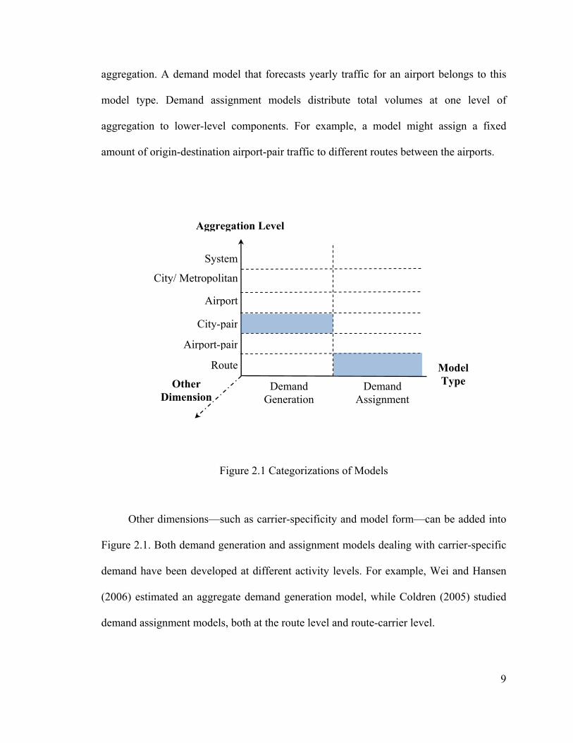
Relevant air transport demand models can be summarized by several dimensions.
Two main dimensions—aggregation level and model type—are shown in Figure 2-1. An
air transport demand model usually analyzes the demand system at a certain level of
aggregation, depending on its purpose of study. For example, an airport demand model
investigates airport activities and provides forecasts for airport planning. Aviation
activities can generally be categorized into following—from high to low aggregation—
levels: system (e.g. world or nation), city or metropolitan, airport, city-pair, airport-pair,
and route. Note that a lower level of activities may be aggregated into higher level
activities. If we know, for instance, traffic on all routes including a particular airport, we
may sum them up to get the activities for the entire airport.
Demand generation and assignment are two main types of models that can be found
in the literature. Demand generation models focus on total demand at a specific level of
aggregation. A demand model that forecasts yearly traffic for an airport belongs to this
model type. Demand assignment models distribute total volumes at one level of
aggregation to lower-level components. For example, a model might assign a fixed
amount of origin-destination airport-pair traffic to different routes between the airports.
Model Type
System
City/ Metropolitan
Airport
City-pair
Airport-pair
Route
Demand Assignment
Demand Generation
Other Dimension
Aggregation Level
Figure 2.1 Categorizations of Models
Other dimensions—such as carrier-specificity and model form—can be added into
Figure 2.1. Both demand generation and assignment models dealing with carrier-specific
demand have been developed at different activity levels. For example, Wei and Hansen
(2006) estimated an aggregate demand generation model, while Coldren (2005) studied
demand assignment models, both at the route level and route-carrier level.
9
10
Models may also be differentiated by form. Broadly, most demand generation
models are regression models, while most assignment models are random utility models.
Random utility models range from simple multinomial logit (e.g. Coldren et al. (2003)),
to nested logit (e.g. Coldren and Koppelman (2005)), and to mixed logit (e.g. Adler et al.
(2005) and Warburg et al. (2006)). Although the sophisticated models may perform better
in explaining travel behavior, the increased complexity generally make them harder to
estimate. In addition, as shown in this research, random utility models can also be used to
predict demand generation.
2.1.2 Demand Generation Model
Demand generation models are older and better developed, compared to demand
assignment models, in the literature. As a result, they are commonly used in practice,
especially for predicting higher level activities. Examples include (1) Federal Aviation
Administration (FAA) (2006), which predicted long-term annual aviation activities for
the U.S. National Airspace System (NAS); (2) Metropolitan Transportation Commission
(MTC) (2001), which projected aviation activities of the San Francisco Bay Area as a
whole and for three major commercial each airports in the region; and (3) FAA’s
“Terminal Area Forecast (TAF)” (2007b), which provided annual enplanement forecasts
at the airport level.
Studies usually model demand as a function of socioeconomic and supply
characteristics, and use either time series or cross-sectional data to estimate parameters.
Higher level models, such as those of above examples, typically rely more on
socioeconomic characteristics (e.g. income and population), and use time series data to
11
estimate the models. Lower level models, on the other hand, are more likely to
incorporate supply characteristics and use either time series or cross-sectional data.
Kanafani and Fan (1974) estimated a city-pair model, which specified population, income,
and travel time as explanatory variables, with cross-sectional data. More recently, Wei
and Hansen (2006) estimated an aggregate generation model with cross-sectional data at
route-carrier level.
Note that models estimated with cross-sectional data assume that the same model
can be used for all units in the cross-section (e.g. airports in airport models, and city-pairs
in city-pair models) in the sample. In order to capture cross-sectional variation, stratifying
the sample may be needed. In addition, this kind of model cannot capture system changes
over time. They, thus, have limited capability to predict future activities. On the other
hand, models estimated with time series data are more suitable for forecasting.
Another issue for this type of model is that the need, at least for the lower level
models, to consider the competitive effects of alternatives. In other words, it is usually
not appropriate to assume that demands are independent across units. Different routes of
the same origin-destination city-pair, for example, are very likely to compete with one
another. Competition among different modes is also important, especially for short-haul
markets. One solution for this issue is to use models, such as “abstract mode model”
developed by Quandt and Baumol (1966). Another common solution is to introduce a
demand assignment model, which will be discussed below.
12
2.1.3 Demand Assignment Model
Demand assignment models explain the distributions of demands among
alternatives. In practice, these models are usually used in top-down traffic forecasting.
Given traffic volumes at a higher unit of aggregation, these models assign traffic volumes
to lower units. For example, a regional planning authority may use an assignment model
to predict the aviation activities in its own region, based on FAA’s national forecasts.
While assignment models for high level of aggregation are usually simple (for
example, analyzing historical shares with adjustments for different scenarios), more
sophisticated assignment models have been developed for assignment to lower level of
aggregation, mainly due to the need for modeling competition effects. In addition, since
the objective of this research is to model the city-pair demand and its assignment to
routes, we only focus on the sophisticated models dealing with lower level activities here.
Three categories of relevant models—airport demand, route demand, and supply-demand
assignment models—are discussed as follows.
Airport Demand Assignment Model
Airport demand assignment models explain the market shares of airports serving
the same region (usually called multiple airport region or multiple airport system in the
literature), such as a big city or metropolitan area. Varieties of model forms, causal
factors, and alternatives (choice sets) have been investigated in the literature.
Discrete choice models are the mainstream model used for airport demand
assignments. Along with the development of discrete choice models, different variations
of this model—including multinomial logit (MNL), nested logit (NL), and mixed
13
multinomial logit (MMNL)—have been applied to this subject. Most of the earlier studies,
such as Harvey (1987), Hansen (1995), and Windle and Dresner (1995), estimated MNL
models to explain airport choice behavior. Although the MNL model form is easily
applied and interpreted, it has the independent of irrelevant alternatives (IIA) property,
which may lead to unreasonable results in some cases. Assume that there are three (A, B,
and C) airports in a metropolitan area. The IIA property implies that an attribute (utility)
change of airport C does not affect the ratio of the probabilities of choosing airport A and
B. However, if the correlation between airport A and C is higher than that between
airport B and C (e.g. airport A and C serve more overlapping markets than airport B and
C do), people would expect that an attribute change of airport C has a larger impact on
probability of choosing airport A than on that of choosing airport B. For example, a low
cost carrier beginning to serve airport C is expected to attract more passengers from
airport A than B, and the ratio of the probabilities of choosing airport A over B is
expected to decrease, rather than staying the same.
The NL and MMNL models provide more realistic results when the IIA property is
violated. The NL model gives more flexible substitution patterns, and still keeps the
computational simplicity of the MNL model. Using the NL models, Pels et al (2001)
analyzed airport-airline choice behavior and Pels et al (2003) modeled airport-access
mode choice behavior. The MMNL model allows for the most flexible substitution
patterns among the three model forms. In addition, it can account for passenger
heterogeneity. More recently, the MMNL models have been applied to allocating airport
demand. Examples include Hess and Polak (2005a and 2005b), and Pathomsiri and
Haghani (2005). Note that the advantages of the MMNL model are not free—they come
14
at the price of computational complexity. The trade-off between flexibility and
complexity does not always favor the most advanced model.
Three causal factors for airport demand assignment models can be found in the
literature—access time, flight frequency, and air fare. Most studies—for example, Harvey
(1987), Windle and Dresner (1995), Pels et al (2001), Pels et al (2003), Basar and Bhat
(2004), Hess and Polak (2005a and 2005b), and Pathomsiri and Haghani (2005)—
specified both access time and flight frequency as their explanatory variables. Although
recognized as a key factor in airport choice (e.g. Ashford and Benchemam (1987), and
Harvey (1987)), air fare was not as widely incorporated as the other two factors. The
main reasons are the data availability and reliability. Harvey (1987) omitted air fare
because there was no information available on fare actually paid by individual travelers.
Pathomsiri and Haghani (2005) mentioned that studies often found an insignificant (or
illogical) effect of air fare on airport choices, due to relatively unreliable data. However,
the insignificant effect was perhaps caused by the endogeneity bias3 of estimations,
especially for those studies using highly aggregated air fare data.
3 Whereas most studies expected the fare coefficients should be negative, the estimated coefficients may be more likely biased towards zero (insignificant) or positive direction, if the air fare variable is endogenous. Possible reasons for the endogeneity bias include simultaneity of supply and demand, and omitted variables. Because airlines may set fares based on some demand side variables—such as traffic flow, demand estimations ignoring simultaneity of supply and demand systems may give results that travelers seem to prefer higher air fares. In addition, higher fares may be due to better services. If a model does not take an important service characteristic into account, the estimated fare coefficient may be affected by the fact that passengers
15
Some studies combine other dimensions of air travel into the airport demand
assignment models by defining alternatives (choice sets). Airport-carrier, airport-access
mode, and airport-carrier-access mode choice models have been developed, for example,
by Pels et al (2001), Pels et al (2003), and Hess and Polak (2005b), respectively. In
addition, Basar and Bhat (2004) parameterized the formation of choice sets, in order to
allow different travelers to have different airport alternatives.
Route Demand Assignment Model
Route demand assignment models explain the market shares of routes serving the
same O-D airport-pair or O-D city-pair4. Similar to the airport demand assignment
models, discrete choice models are the mainstream models used for route demand
assignments. Note that assigning O-D airport-pair traffic to routes assumes that there are
no substitution effects between routes of different O-D airport-pairs, even though these
routes serve the same O-D city-pair.
The route demand assignment model for city-pairs, which combines the airport
demand assignment for multiple airport regions and the route demand assignment for
airport-pairs, is of interest when the study area includes multiple airport systems (MAS).
Kanafani and Fan (1974), and Kanafani et al (1977) developed route demand assignment
models for the San Francisco- Los Angles city-pair. Both of the cities are served by
prefer better services (measured by the characteristic). Therefore, both simultaneity and omitted variables may lead the estimated coefficients that are biased upward.
4 An airport-pair is equivalent to a city-pair only if both the origin and destination of the city-pair are served by single airport.
16
multiple airports. Total travel time (including airport access time), air fare, and flight
frequency were used in their models to explain the market share differences among the
routes. As for model forms, Kanafani and Fan (1974) designed a special probabilistic
form and Kanafani et al (1977) applied the (aggregate) MNL model.
Compared to those for city-pairs, more route demand assignment models for
airport-pairs can be found in the literature. Some studies assign airport-pair traffic to
carriers and routes. For example, Coldren et al. (2003) estimated a MMNL model, and
Coldren and Koppelman (2005) applied a NL model for route-carrier demand
assignments. Both of these used computer reservation systems data from a commercial
source. In addition, Adler et al. (2005) and Warburg et al. (2006) used revealed- and
stated-preference survey data from individual travelers to estimate the mixed logit models
that account for the heterogeneity of travelers in route-carrier choices.
In addition to the pure demand assignment model, some studies have developed
models with both supply and demand sides. Studies with this approach are discussed
below.
Supply-Demand Model
The supply-demand models are usually composed of a discrete travelers’ choice
sub-model for predicting demands, and an optimization sub-model of airlines’ behavior.
The most widely used discrete choice model for this topic is the multinomial logit (MNL)
model, whereas the nested logit (NL) model is also applied by other studies (e.g. Hansen
(1996), Weidner (1996), and Hsiao and Hansen (2005)). Examples of applying the MNL
model include Kanafani and Ghobrial (1985), Hansen (1990), Hansen and Kanafani
17
(1990), Ghobrial and Kanafani (1995), Hansen (1995), Adler (2001), and Adler (2005).
Note that all the models mentioned in this sub-section are route demand assignment
models for airport-pairs, except for Hansen’s (1995) model, which is an airport demand
assignment model.
To capture airlines’ behavior, some studies, which often focus on airline
competition issues, apply an optimization model and assume that airlines pursue maximal
profits as their objective functions. Hansen (1990), Adler (2001), Adler (2005), and Hsu
and Wen (2003) are examples of such studies. Instead of an optimization model, other
approaches have been used in order to incorporate the supply side of the system. For
instance, Kanafani and Ghobrial (1985) assigned the maximum frequency of service on
each link subject to the load factor above the breakeven load factor on that link.
These supply-demand models reflect the behavior of travelers and airlines, and thus
they may offer better understanding of the systems. However, these models are usually
more complicated and may take a long time to equilibrate. Especially for models with
integer programming sub-models, it is harder to implement these models on large scale
networks, such as the whole domestic air transportation network of the United States.
2.1.4 Discussion and Summary
In this section, strengths and weaknesses of different models, including models in
the literature and the proposed model, are discussed by model components: model type
and aggregation level, model form, choice set, and data issues. Finally, features of these
models are summarized.
18
Model Type and Aggregation Level
Since lower level activities may be aggregated into higher level activities, a model
of lower aggregation level can be more flexible for practical applications and also can
better explain air travel behavior. For example, the impacts of raising passenger segment
fees5 on route and airport demand can be more accurately estimated by a route demand
model, rather than an airport demand model, since a route demand model can better
capture a traveler’ choice of connecting airports. Lower level aggregation models must
take competition effects of alternatives into account. Although demand assignment
models can be used to capture the competition effects, they implicitly assume total
demand is inelastic. Demand generation models enable total demand to change with
characteristics of alternatives. Thus, a model combines both demand generation and
demand assignment is preferable.
In the literature, most air travel studies only deal with either demand generation or
demand assignment. Researchers may estimate these two types of models separately and
apply these models sequentially—generating demands at one level of aggregation and
then distributing the estimated volumes to lower-level components. For instance,
Kanafani and Fan (1974) estimated demand generation and demand assignment models
for the San Francisco-Los Angles city-pair—generated the city-pair demand first, and
then distributed the total volume to different routes between these two cities. However,
5 Air passengers are charged the segment fees based on the number of flight segments of
their routes. For example, if the current fee is 3 dollars per segment, a passenger choosing a direct route only pays a 3 dollar fee. However, if the passenger chooses a one-stop route, he or she pays 6 dollars for the segment fee.
19
the sequential approach that does not include a feedback system may be problematic,
because it implicitly assumes that the total volume is fixed for the assignment model.
Adding a feedback system can improve the sequential approach; however, this needs
more complicated model systems and consumes more computation time. A model dealing
with demand generation and assignment simultaneously can be a better solution.
This research models air travel demand at the route level and simultaneously deals
with demand generation and assignment. The proposed model is consistent with random
utility theory. For air travel activities at a lower aggregation level, city-pair models are
suitable for estimating demand. They are also the most common demand generation
models in the literature, according to Kanafani (1983). This research, therefore, develops
the model that generates city-pair demands and distributes them to routes, as the shaded
areas shown in Figure 2-1. In addition, the model combines airport and route choices in
demand assignment, since both origin and destination cities may be served by multiple
airports.
Model Form
Discrete choice models—including the MNL, NL, and MMNL models—are the
usual demand assignment models. The MNL model is widely used although its IIA
property may lead to unreasonable results. The MMNL model provides the most flexible
substitution patterns but increases the computational complexity. The NL model gives for
more flexible substitution patterns, and still keeps the computational simplicity. Although
these three model forms are all available in theory, researchers should make their own
20
choices depending on their problems and objectives. In this regard trade-offs between the
flexibility and complexity must be considered.
This research chooses the aggregate NL model (and also estimate the aggregate
MNL6 model for comparisons) for the empirical study, because: (1) the empirical
objective of this research focuses on the coefficients and ratios of coefficients, and the
NL model can serve this purpose well7, and (2) the NL model provides a good balance
between flexibility and computational complexity. There is a need to reduce the
computational complexity because the empirical study uses the U.S. domestic route data
for 40 quarters, which is a very large data set (about 1.66 million observations), allowing
us to investigate air demand variation among routes and markets over time.
Choice Set
Most of the demand assignment models in the air travel literature, except Hong and
Harker (1992), Adler (2001), and Adler (2005), do not include an “outside good”
alternative, which allows a potential traveler to choose none of the listed alternatives. In
an air route choice case, a potential traveler may not travel (or travel by other modes,
6 Note that when individuals are homogeneous, the IIA property also holds at the
aggregate level. In this case, the properties of aggregate own and cross elasticities are similar to those of disaggregate own and cross elasticities. Refer to Ben-Akiva and Lerman (1985) for details about the IIA property and the differences between disaggregate and aggregate elasticities.
7 For instance, Brownstone and Train (1999) mentioned that “If indeed the ratios of coefficients are adequately captured by a standard logit model, as our results and those of Bhat (1996a) and Train (1998) indicate, then the extra difficulty of estimating a mixed logit or a probit need not be incurred when the goal is simply estimation of willingness to pay, without using the model for forecasting.”
21
such as car or rail) if none of the route alternatives is as attractive as that option. However,
a route choice model without the “outside good” alternative forces the potential traveler
to pick one of the routes.
A demand assignment model without an “outside good” alternative implies that
total demand is independent of the attributes of the disaggregate alternatives. These
attributes affect market shares among alternatives, rather than the total demand. This
property restricts the application of the model as a planning and policy analysis tool,
since a system improvement may lead to changes in total demand. Our research takes the
“outside good” alternative into consideration.
Data Issues
In this section, two data issues are discussed: aggregation levels (aggregate and
individual data), and data dimensions (cross-sectional, time series, and panel data).
Most demand generation models in the literature use aggregate time series data,
while some lower activity level generation models may use aggregate cross-sectional data.
On the other hand, most demand assignment (including airport and route assignment)
models using discrete choice model forms are estimated by cross-sectional data, either
from surveys of individuals, or from aggregate statistics8. While airport choice models
typically use cross-sectional data from surveys of individuals, route choice models are
8 Discrete choice models estimated by aggregate data are sometimes referred as market
share models, or aggregate choice models (e.g. aggregate multinomial logit model). The supply-demand models usually apply the market share models to their demand assignments.

22
more likely to be estimated by aggregate statistics, since it is easier to do a survey in a
single metropolitan area than at a national level.
Surveys of individuals can collect more detailed information. The models estimated
on survey data, thus, may better explain travel behavior, if the surveys are well designed.
However, due to their costly nature, survey data is usually limited in terms of sample size
and geographical area, reducing generalizability of estimation results. For instance, an
airport choice model estimated by San Francisco Bay Area data may not apply to other
metropolitan areas. In addition to its scarcity, problems with surveys of individuals
include limited public availability and their inability to track changes over time.
Aggregate statistics, by contrast, are usually available for different geographical areas
and reported on a regular basis, enabling the use of panel data analysis techniques.
This research builds a route level model that can be applied to a large airline
network—such as the whole U.S. air transportation system—as a bottom-up policy
analysis tool. Survey data for this type of empirical analysis is unavailable. Publicly
available aggregate (route level) data is employed. Since these data are collected and
reported on a regular basis, it is possible to access changes in the structure of air travel
demand over time, as well as to fuse inferences on both cross-sectional and time series
variation.
23
Summary
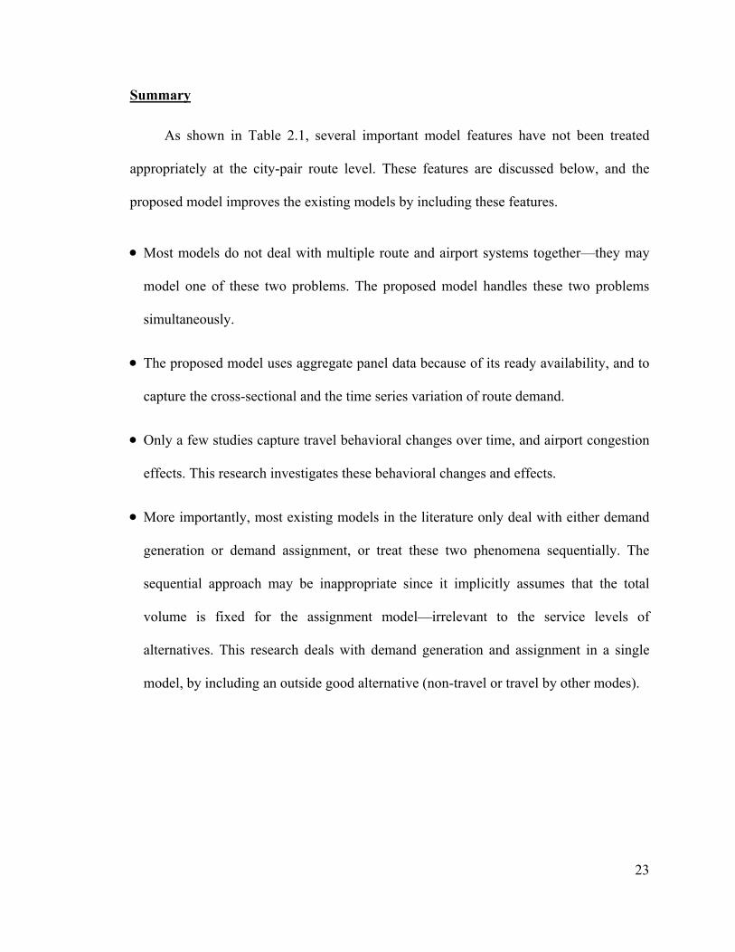
As shown in Table 2.1, several important model features have not been treated
appropriately at the city-pair route level. These features are discussed below, and the
proposed model improves the existing models by including these features.
• Most models do not deal with multiple route and airport systems together—they may
model one of these two problems. The proposed model handles these two problems
simultaneously.
• The proposed model uses aggregate panel data because of its ready availability, and to
capture the cross-sectional and the time series variation of route demand.
• Only a few studies capture travel behavioral changes over time, and airport congestion
effects. This research investigates these behavioral changes and effects.
• More importantly, most existing models in the literature only deal with either demand
generation or demand assignment, or treat these two phenomena sequentially. The
sequential approach may be inappropriate since it implicitly assumes that the total
volume is fixed for the assignment model—irrelevant to the service levels of
alternatives. This research deals with demand generation and assignment in a single
model, by including an outside good alternative (non-travel or travel by other modes).
24
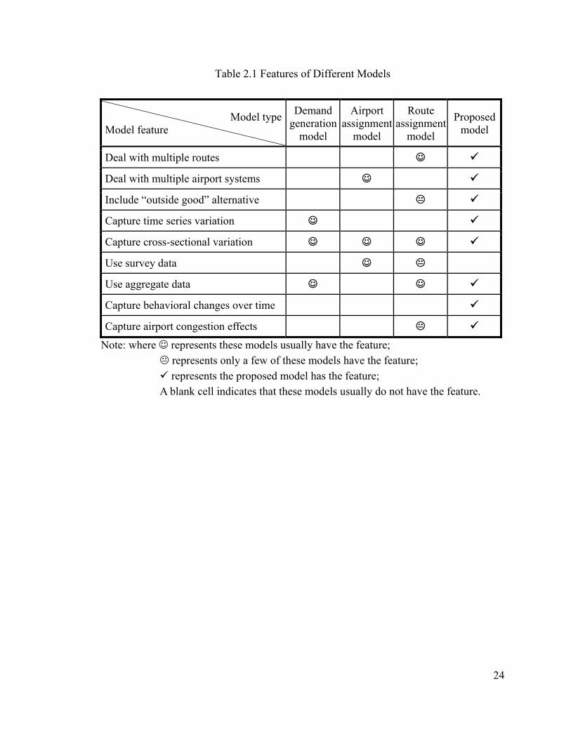
Table 2.1 Features of Different Models
Model typeModel feature
Demand generation
model
Airport assignment
model
Route assignment
model Proposed
model
Deal with multiple routes ☺ Deal with multiple airport systems ☺
Include “outside good” alternative Capture time series variation ☺
Capture cross-sectional variation ☺ ☺ ☺ Use survey data ☺ Use aggregate data ☺ ☺
Capture behavioral changes over time
Capture airport congestion effects Note: where ☺ represents these models usually have the feature;
represents only a few of these models have the feature; represents the proposed model has the feature;
A blank cell indicates that these models usually do not have the feature.
25
2.2 The Demand Model
2.2.1 Conceptual Framework
This research models city-pair air passenger demand at the route level9. In general,
potential trips between two cities are derived from the socioeconomics activities in both
cities. Potential travelers may have many choices regarding these potential trips. They
may avoid air travel altogether by choosing different modes, such as auto and rail, or they
may decide not to travel at all. Within the air mode, they may select different routes, of
which airports and segments (non-stop links) are basic elements. Thus, a route choice
involves choices of airports (origin, destination, and connecting airports) and segments. A
change in the characteristics of a route may affect the attractiveness of this route, or of a
group of routes, because different routes in a market may share the same airports and/or
segments. Aggregate air demand in a city-pair market may also be affected by changes in
individual route characteristic or that impact routes across the board.
Intercity travel demand can be illustrated by an example of one city-pair (A-B), as
shown in Figure 2.2. Potential travelers in this market have one “outside good”
alternative (non-travel or travel by other modes) and 11 route alternatives, including three
non-stop routes (O1D2, O2D1, and O3D2) and eight one-stop routes (four for each of the
connecting airports, H1 and H2). From the airport view point, since both city A and B
9 Note that this conceptual model can be easily applied to the route-carrier level—simply
differentiating routes by carriers. However, adding the carrier dimension yields to a more complicated empirical model.
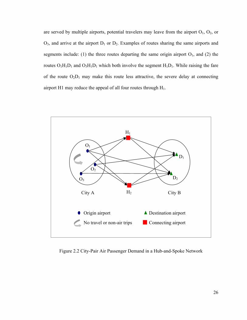
are served by multiple airports, potential travelers may leave from the airport O1, O2, or
O3, and arrive at the airport D1 or D2. Examples of routes sharing the same airports and
segments include: (1) the three routes departing the same origin airport O1, and (2) the
routes O1H1D1 and O3H1D1 which both involve the segment H1D1. While raising the fare
of the route O2D1 may make this route less attractive, the severe delay at connecting
airport H1 may reduce the appeal of all four routes through H1.
H1
Origin airport
Connecting airport
City A City B
Destination airport
D1
D2 O3
O2
O1
H2
No travel or non-air trips
Figure 2.2 City-Pair Air Passenger Demand in a Hub-and-Spoke Network
26
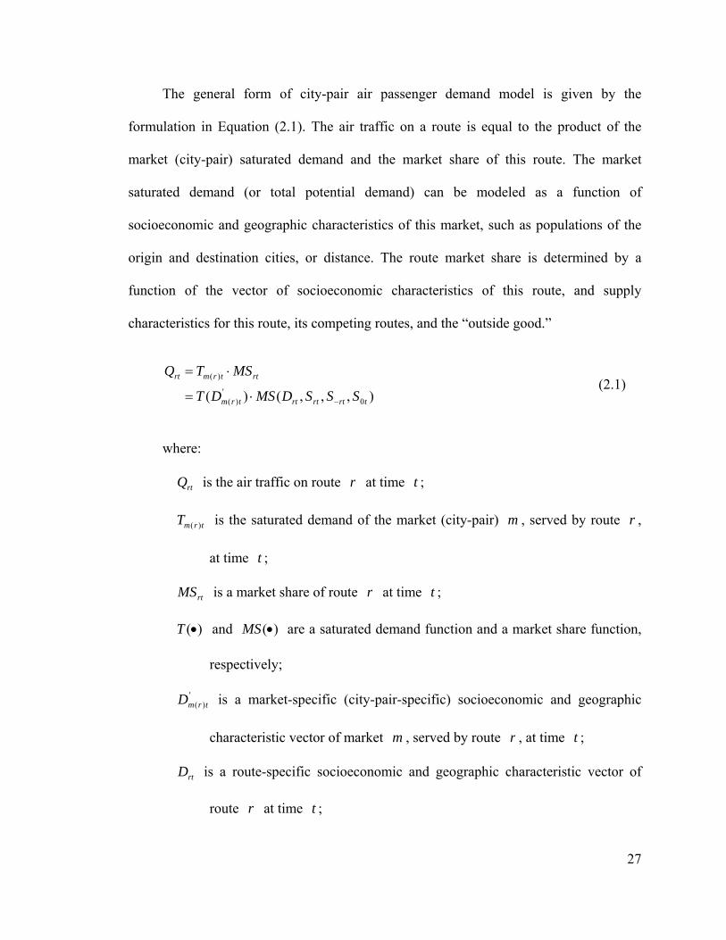
The general form of city-pair air passenger demand model is given by the
formulation in Equation (2.1). The air traffic on a route is equal to the product of the
market (city-pair) saturated demand and the market share of this route. The market
saturated demand (or total potential demand) can be modeled as a function of
socioeconomic and geographic characteristics of this market, such as populations of the
origin and destination cities, or distance. The route market share is determined by a
function of the vector of socioeconomic characteristics of this route, and supply
characteristics for this route, its competing routes, and the “outside good.”
),,,()( 0'
)(
)(
trtrtrttrm
rttrmrt
SSSDMSDT
MSTQ
−⋅=
⋅= (2.1)
where:
rtQ is the air traffic on route r at time ; t
trmT )( is the saturated demand of the market (city-pair) , served by route m r ,
at time ; t
rtMS is a market share of route r at time t ;
)(•T and are a saturated demand function and a market share function,
respectively;
)(•MS
')( trmD is a market-specific (city-pair-specific) socioeconomic and geographic
characteristic vector of market , served by route m r , at time ; t
rtD is a route-specific socioeconomic and geographic characteristic vector of
route r at time ; t
27
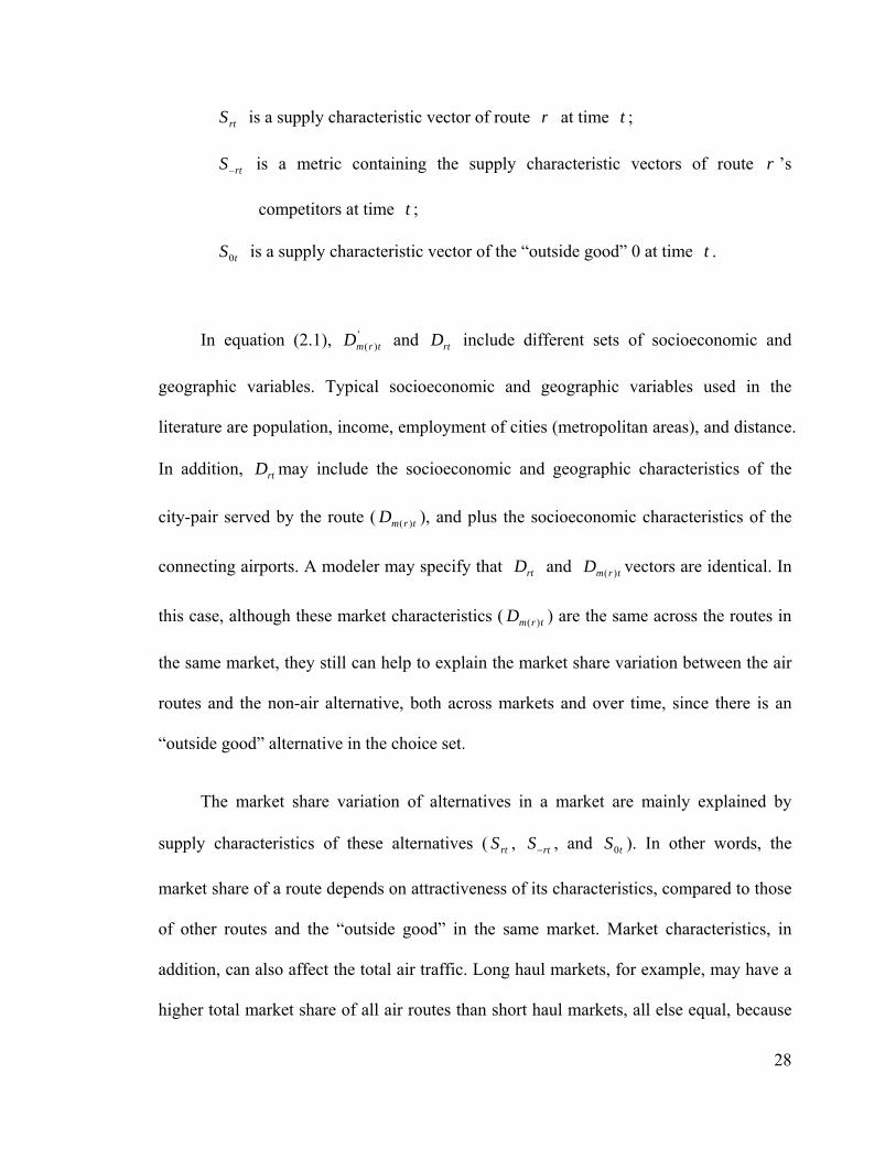
rtS is a supply characteristic vector of route r at time ; t
rtS− is a metric containing the supply characteristic vectors of route r ’s
competitors at time ; t
tS0 is a supply characteristic vector of the “outside good” 0 at time . t
In equation (2.1), and include different sets of socioeconomic and
geographic variables. Typical socioeconomic and geographic variables used in the
literature are population, income, employment of cities (metropolitan areas), and distance.
In addition, may include the socioeconomic and geographic characteristics of the
city-pair served by the route ( ), and plus the socioeconomic characteristics of the
connecting airports. A modeler may specify that and vectors are identical. In
this case, although these market characteristics ( ) are the same across the routes in
the same market, they still can help to explain the market share variation between the air
routes and the non-air alternative, both across markets and over time, since there is an
“outside good” alternative in the choice set.
')( trmD
D
rtD
rtD
trm )(
rtD
trmD )(
trmD )(
The market share variation of alternatives in a market are mainly explained by
supply characteristics of these alternatives ( , , and ). In other words, the
market share of a route depends on attractiveness of its characteristics, compared to those
of other routes and the “outside good” in the same market. Market characteristics, in
addition, can also affect the total air traffic. Long haul markets, for example, may have a
higher total market share of all air routes than short haul markets, all else equal, because
rtS rtS− tS0
28
there is less competition among modes in long haul markets. Recall that airports and
segments are basic elements of a route. Supply characteristic vectors of routes should be
composed of characteristics of these routes, and of the airports and segments involved.
Using as an example, it can be decomposed into three parts:
where and are characteristic vectors of the airports and the segment (s)
served by route
rtS
raS (
},,{ )()('
trgtrartrt SSSS = ,
t) trgS )(
r at time t , respectively; is a pure route characteristic vector of
route
'rtS
r at time . Typical supply characteristic variables include: air fare, travel time,
and routing types (pure route variables), ground access time and airport delay (airport
variables), and flight frequency (a segment variable).
t
The saturated demand and the market share functions give the total potential traffic
of a market and the market share of a route (or the outside good), respectively, when all
socioeconomic, geographic and supply variables are given. Although these functions are
specified and estimated in the later chapters, the methodological issues in using them are
discussed in the following two sections.
2.2.2 Saturated Demand Function
The saturated demand function defines the relationship between the total potential
demand of markets and certain causal factors. Whereas socioeconomic variables are
easily justified as the causal factors for the saturated demand, estimating the function may
not be straightforward because only the realized traffic, rather than the “potential” traffic,
can be observed. From the economic literature, two types of approaches have been
proposed by empirical studies on different industries.
29
The first approach, which is more commonly found in the literature, is to assume a
reasonable maximum for the potential based on a socioeconomic variable. For example, a
researcher may assume trmtrm MT )()( *α= , where α is a proportionality factor and
is the observable socioeconomic variable chosen for reflecting the potential total
traffic. Nevo (2001) analyzed the market shares of different brands on the ready-to-eat
cereal industry. The potential number of servings in a city in a quarter was defined as a
function of population,
trmM )(
α *(population)*365/4. The potential number of servings was
calculated by assuming α =1, i.e., every resident may consume one serving per day. The
main advantage of this approach is its simplicity. However, in order to provide
convincing results, justification and coefficient sensitivity tests for this assumption are
needed.
The second approach is to estimate a model for this function (e.g. estimate the
parameter α ). Because the saturated demand is a part of the whole demand model and
the “potential” traffic cannot be observed, estimating the saturated demand model is more
complicated. System equations and/or additional assumptions to simplify the estimation
may be used by this approach. For example, Hansen (1996), and Wei and Hansen (2005)
assumed that the total demand is much more than the total traffic in a market, and then
separated the estimation of the saturated demand model from that of the whole demand
model.
30
This research would suggest the first approach for the proposed model. Even
though this approach is simple, it can be shown10—at least for the multinomial logit and
nested logit model forms—that the proportionality factor setting may only affect the
estimated intercept of the market share model if the proportionality factor is set large
enough. If the intercept is not the main coefficient of interest, this approach should work
well. In addition, socioeconomic variables in the market share model ( ) can help to
explain the market share difference between all routes and the outside good. Thus, the
impacts of choosing an inappropriate parameter (e.g.
rtD
α ) and socioeconomic variables
for can be reduced. ')( trmD
2.2.3 Market Share Function
Whereas alternative methods exist in the literature11, the usual specification for the
market share function is a discrete choice model. Only this type of model is discussed in
this section, since the empirical analysis of the research reported here follows the discrete
choice literature. To be specific, the aggregate discrete choice models, which are based
on choice behavior of individuals, are the focus of our interest. This type of model is the
most appropriate for the objectives of this research: to develop a route demand model,
10 Refer to Appendix A for more details. 11 For example, some studies directly explained the market share (as a dependent
variable) by causal factors using a linear regression model, or a multiplicative model. Other studies transformed the dependent variable to assure that the predicted market share is between 0 and 1.
31
which can be applied to a large network system, using publicly available aggregate (at the
route level) data.
The indirect utility of potential traveler i from route r at time can be
formulated as Equation (2.2),
t
irtirtrt
K
krtkkirt xu εμξβ +++= ∑
=1
, (2.2)
where:
rtkx is an observable characteristic of route k r at time , i.e., it is a
observable supply characteristic variable in vector ; there are
t
rtS K
observable characteristics specified in the utility function;
kβ is a parameter to be estimated for characteristic ; k
rtξ is a term to capture unobservable route characteristics at time ; t
irtμ is a term to capture individual deviations, which can be modeled as a
function of individual characteristics and route characteristics;
irtε is a stochastic term.
In order to derive the market share function for route r at time t , additional
assumptions are needed12. The first assumption is that every potential traveler chooses
only one alternative that gives the highest utility from all alternatives (including the
12 Further discussions and formulas can be found in the discrete choice literature (e.g.
McFadden (1981)) and its applications, such as Berry et al (1995) and Nevo (2001).
32
“outside good,” and all the routes). This assumption allows us to define the set of
unobserved variables ( ) that induces the choice of route rtA r at time . Note that this
assumption may be unrealistic for analyzing general products. For example, a consumer
may purchase two products at the same time, or may consider the choice between two
small size items of a brand and one large size item of another brand. However, this
assumption is easier to justify in the route choice model, since for each realized trip a
traveler always travel through only one route.
t
Assuming ties occur with zero probability, the market share of route r at time t
as a function of the characteristics of all alternatives competing in the market is given by
integrating the population distribution functions of unobserved variables over the range
of . An operational market share function needs to make assumptions on the
population distribution functions, and then the integral can be calculated. Different
assumptions on the population distribution functions lead to different discrete choice
models. Three models—MNL, NL, and MMNL—are discussed below.
rtA
Multinomial Logit Model
The most frequent and simple way is to assume that (1) potential travelers are
homogeneous in the observed characteristics—no individual deviations ( 0=irtμ ) except
for the stochastic terms irtε ’s ; and (2) the stochastic terms, irtε ’s, are independent and
identically distributed (i.i.d.) across travelers, routes, and time with a type I extreme value
distribution. This leads to the multinomial logit model, which captures the mean behavior
33
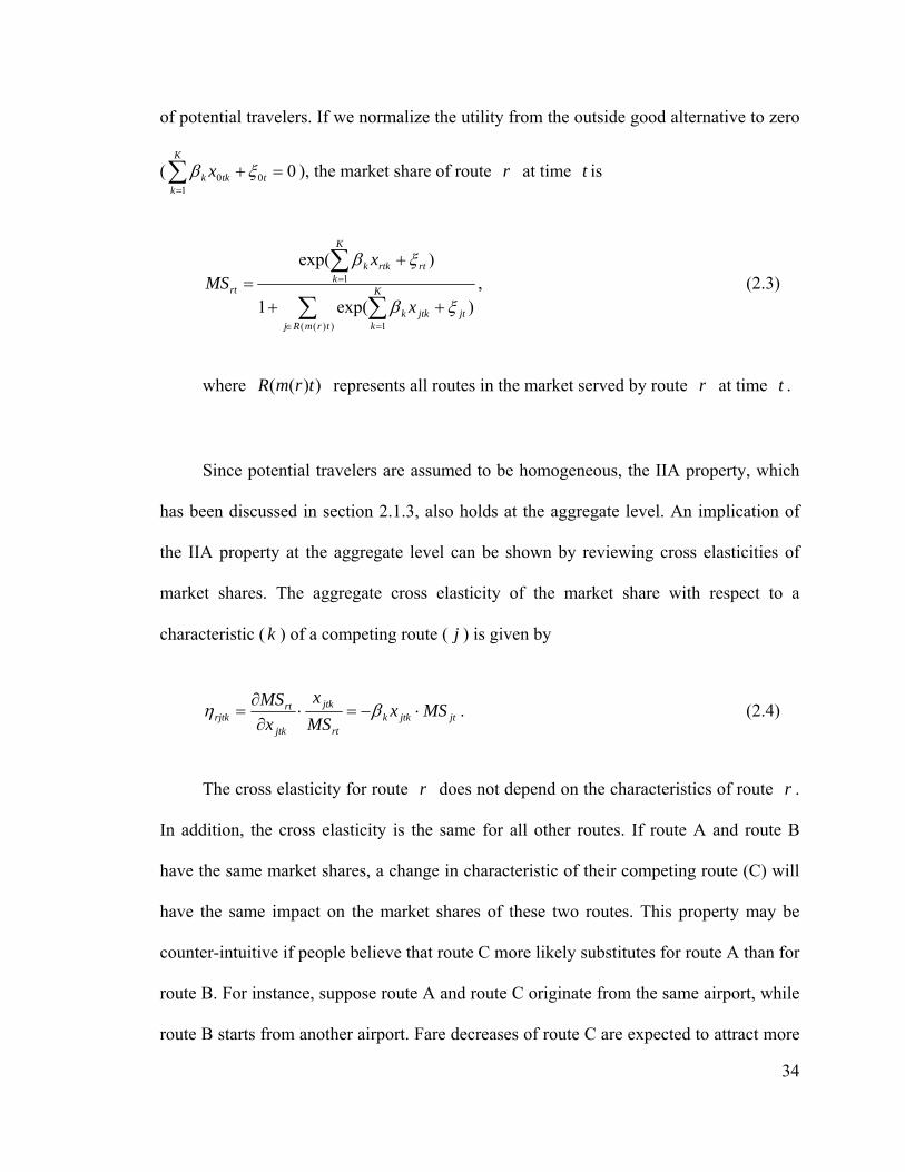
of potential travelers. If we normalize the utility from the outside good alternative to zero
( ), the market share of route 001
0 =+∑=
t
K
ktkk x ξβ r at time is t
∑ ∑
∑
∈ =
=
++=
1Rj
rtMS
(( rmR
+
))(( 1
1
)exp(
)exp(
trmjt
K
kjtkk
rt
K
krtkk
x
x
ξβ
ξβ, (2.3)
where represents all routes in the market served by route ))t r at time t .
Since potential travelers are assumed to be homogeneous, the IIA property, which
has been discussed in section 2.1.3, also holds at the aggregate level. An implication of
the IIA property at the aggregate level can be shown by reviewing cross elasticities of
market shares. The aggregate cross elasticity of the market share with respect to a
characteristic ( ) of a competing route ( j ) is given by k
jtjtkkrt
jtk
jtk
rtrjtk MSx
MSx
xMS
⋅−=⋅∂∂
= βη . (2.4)
The cross elasticity for route r does not depend on the characteristics of route r .
In addition, the cross elasticity is the same for all other routes. If route A and route B
have the same market shares, a change in characteristic of their competing route (C) will
have the same impact on the market shares of these two routes. This property may be
counter-intuitive if people believe that route C more likely substitutes for route A than for
route B. For instance, suppose route A and route C originate from the same airport, while
route B starts from another airport. Fare decreases of route C are expected to attract more
34
35
passengers from route A than from route B. However, the MNL model predicts the same
market share changes for route A and route B.
Nested Logit Model
The NL model gives more flexible substitution patterns, and still keeps the
computational simplicity and tractability of the MNL model. In the NL model, all
alternatives are grouped into exhaustive and mutually exclusive nests. According to the
nest structure, the correlations of the stochastic terms in the NL model are specified by a
variance component structure, instead of assuming that the stochastic terms are i.i.d.. As a
result of the specification, the IIA property does not hold across nests, although it still
holds within each nest. Thus, the substitution patterns of alternatives become more
flexible. An alternative is more likely to substitute for an alternative in the same nest,
than for an alternative in different nests. In the route choice example above, if route A
and C are in the same nest and route B is in another nest, the NL model predicts, as one
would expect, that fare decreases of route C attract more passengers from route A than
from route B.
Note that the NL model can be decomposed into multinomial logit models13, since
the probability of choosing an alternative can be written as the product of a marginal and
a conditional probability—each of them takes the multinomial logit form. Assuming the
potential travelers are homogeneous, the decomposition can also be applied to the
13 Refer to Train (2003) for details.
36
aggregate level14—replacing the probabilities by market shares. The decomposition
makes the interpretation of the NL model easier and also provides an alternative for
model estimation.
Two additional attributes of the NL model are worthy of mention. The first is that
when all correlations of the stochastic terms are zero the NL model becomes the MNL
model. Thus, the MNL model is a special case of the NL model. The other important
attribute is that, like the MNL model, the market shares of the NL model have a closed
form expression—no numerical method for the market share integral is needed. No
market share equation for a NL model provided here because it depends on the nest
structure. However, it can be decomposed, in general, into marginal and conditional
market shares. Equations similar to (2.3) can be used for these marginal and conditional
market shares. Then, the market share of a route can be determined. All above attributes
make the NL model popular for empirical studies.
One issue of the NL model is that the nesting structure, including contents of nests
and order of nests, has to be determined. In our route choice model, since different routes
of a market may share the same airports and/or segments, routes can be grouped by their
common characteristics. Although this provides a priori information on the possible nest
structure, the final nesting structure needs to be determined empirically as discussed in
the next chapter.
14 Berry (1994) showed the decomposition for a two level aggregate nested logit model.
Mixed Logit Model
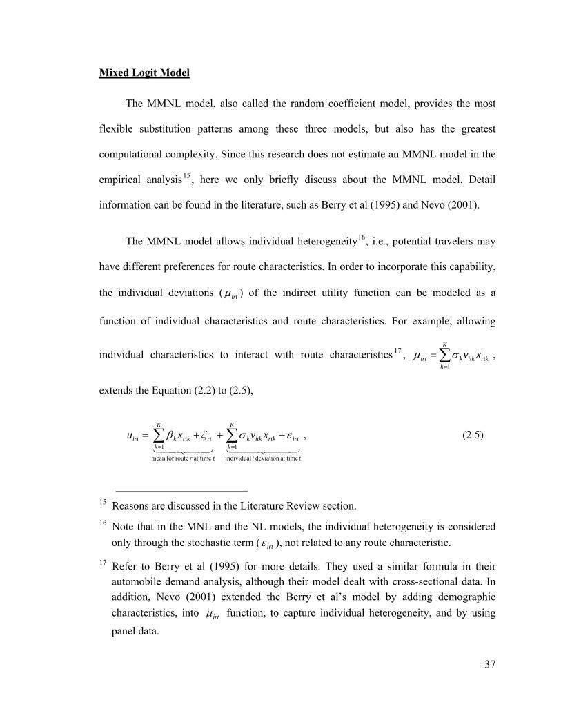
The MMNL model, also called the random coefficient model, provides the most
flexible substitution patterns among these three models, but also has the greatest
computational complexity. Since this research does not estimate an MMNL model in the
empirical analysis15, here we only briefly discuss about the MMNL model. Detail
information can be found in the literature, such as Berry et al (1995) and Nevo (2001).
The MMNL model allows individual heterogeneity16, i.e., potential travelers may
have different preferences for route characteristics. In order to incorporate this capability,
the individual deviations ( irtμ ) of the indirect utility function can be modeled as a
function of individual characteristics and route characteristics. For example, allowing
individual characteristics to interact with route characteristics 17 , ,
extends the Equation (2.2) to (2.5),
∑=
=K
krtkitkkirt xv
1σμ
44 344 214434421ti
irt
K
krtkitkk
tr
rt
K
krtkkirt xvxu
at timedeviation individual
1
at time routefor mean
1εσξβ +++= ∑∑
==
, (2.5)
15 Reasons are discussed in the Literature Review section. 16 Note that in the MNL and the NL models, the individual heterogeneity is considered
only through the stochastic term ( irtε ), not related to any route characteristic.
17 Refer to Berry et al (1995) for more details. They used a similar formula in their automobile demand analysis, although their model dealt with cross-sectional data. In addition, Nevo (2001) extended the Berry et al’s model by adding demographic characteristics, into irtμ function, to capture individual heterogeneity, and by using
panel data.
37
where:
itkv is a mean zero random variable, associated with route characteristic for
individual at time , with a known distribution;
k
i t
kσ is a parameter to be estimated, and represents the standard deviation of the
marginal utilities associated with route characteristic , if is scaled
such that .
k itkv
1)( 2 =itkvE
In Equation (2.5) the indirect utility of potential traveler from route i r at time
can be decomposed into two parts: the mean for route t r at time t , and the deviation
from the mean for the potential traveler at time t . For the potential traveler , the
marginal utility associated with route characteristic at time is given by
i i
k t
)itkkk v( σβ + . Assuming the stochastic term, irtε ’s, are independent and identically
distributed (i.i.d.) across travelers, routes, and time with a type I extreme value
distribution, leads to the MMNL model.
Note that the NL model is a restricted version of the MMNL model (Berry et al
(1995)). However, the advantages of the MMNL model come with the price of
computational complexity, because the integral defining market shares of the MMNL
model cannot be computed analytically. Numerical methods are needed to determine the
market shares.
38
39
Chapter 3 Empirical Analysis of the Passenger Demand for Air
Transportation
This chapter shows how the proposed model will be implemented. Model
specifications, including model forms, nesting structures, and causal factors, are
discussed first. Then information about data sources, data compilation, and summary
statistics is provided. Estimation methods and estimation results are presented at the end
of the chapter.
3.1 Model Specifications
3.1.1 Model Forms and Nesting Structures
As discussed in chapter 2, this research chooses the aggregate nested logit (NL)
form for the market share function, and also estimates the aggregate multinomial logit
(MNL) model for comparisons. For the nesting structures of the models, routes are
grouped in a nest by assuming that the routes with more common characteristics are more
likely to be competitors, i.e. higher correlations among these routes. The common
characteristics used in the empirical analysis include (1) air routes or the non-air
alternative, (2) origin-destination (O-D) airport pair, and (3) routing type (direct or
connecting route). Based on different combinations of these characteristics, five nesting
structures are examined—including one MNL, one two-level NL, two three-level NL,
and one four-level NL model.
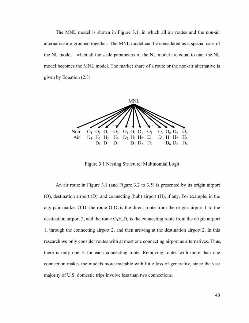
The MNL model is shown in Figure 3.1, in which all air routes and the non-air
alternative are grouped together. The MNL model can be considered as a special case of
the NL model—when all the scale parameters of the NL model are equal to one, the NL
model becomes the MNL model. The market share of a route or the non-air alternative is
given by Equation (2.3).
Non- Air
O1 D1
MNL
O1 D2
O1 H1 D1
O1 H2 D1
O1 H1 D2
O1 H2 D2
Oo Hh Dn
Oo H2 Dn
Oo H1 Dn
Oo Dn
… … … … O1 Hh D2
O1 Hh D1
Figure 3.1 Nesting Structure: Multinomial Logit
An air route in Figure 3.1 (and Figure 3.2 to 3.5) is presented by its origin airport
(O), destination airport (D), and connecting (hub) airport (H), if any. For example, in the
city-pair market O-D, the route O1D1 is the direct route from the origin airport 1 to the
destination airport 2, and the route O1H2D2 is the connecting route from the origin airport
1, through the connecting airport 2, and then arriving at the destination airport 2. In this
research we only consider routes with at most one connecting airport as alternatives. Thus,
there is only one H for each connecting route. Removing routes with more than one
connection makes the models more tractable with little loss of generality, since the vast
majority of U.S. domestic trips involve less than two connections.
40
While the four NL models are presented in following individual sub-sections, their
common features—ratio(s) of scale parameters and model decompositions—are
discussed here. The estimated ratio(s)18 of scale parameters of an NL model can be used
to determine whether the nested logit model is consistent with utility-maximizing
behavior 19 for all possible values of the explanatory variables, and whether the
higher-level NL model collapses to a lower-level NL (or MNL) model. Specific
conditions of the ratio(s) of scale parameters are discussed in each nesting structure
sub-section.
As mentioned in chapter 2, the NL model can be decomposed into multinomial
logit models, since the market share of a route can be written as the product of a marginal
market share and a conditional market share—each of them takes the multinomial logit
form. To illustrate the decompositions of the NL models, the indirect utility of a potential
traveler from route i r at time , Equation (2.2), is expressed as Equation (3.1),
assuming that potential travelers are homogeneous in the observed characteristics—no
individual deviations (
t
0=irtμ ) except for the stochastic terms irtε ’s.
irtc
rtd
rtptmt
irtrtptmt
irtirtrt
K
krtkkirt
YYZW
YZW
xu
ε
ε
εμξβ
++++=
+++=
+++=∑=1
, (3.1)
18 Only the ratio of two scale parameters, rather than each individual scale parameter,
can be identified from the data. 19 Refer to Train (2003) and Ben-Akiva and Lerman (1985) for details.
41

where:
mtW represents the market-specific utility of route r , which is the same for all
routes in the market at time t ; m
ptZ represents the O-D airport pair-specific utility of route r , which is the same
for all routes of the O-D airport pair p at time t ;
rtY is the route-specific utility, which varies over routes in the market at
time ;
m
t
drtY is the route-specific utility for a direct route , which varies over routes in the
market at time for the direct route; ; m t rrtd
rt dYY ⋅=
crtY is the route-specific utility for a connecting route, which varies over routes in
the market at time t for the connecting route; ; m )1( rrtc
rt dYY −⋅=
rd is the binary indicator variable for the direct route;
. { routedirect a is route theif ,1otherwise ,0
rdr =
The second equality in this equation decomposes the utility into three parts: the
market-specific utility, the O-D airport pair-specific utility, and the route-specific utility.
This helps to separate the non-air alternative from the air routes, and to distinguish air
routes between different O-D airport pairs. The third equality further differentiates the
route-specific utility between the direct and the connecting routes. This helps to explain
42
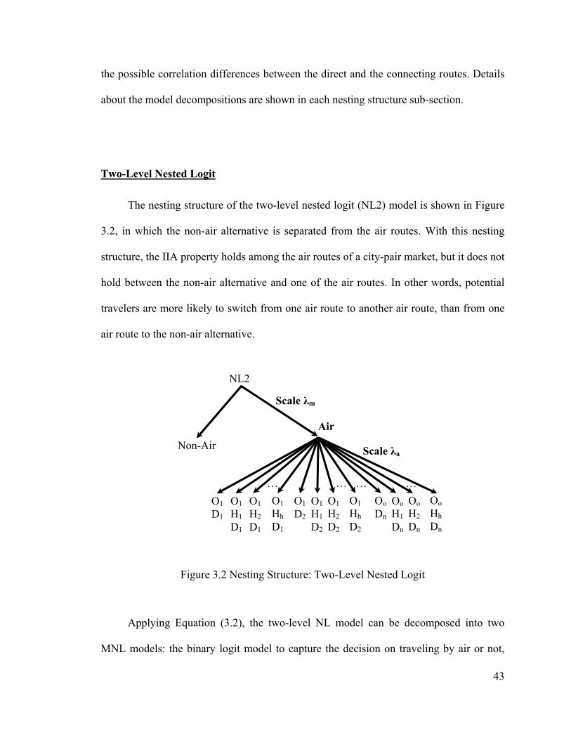
the possible correlation differences between the direct and the connecting routes. Details
about the model decompositions are shown in each nesting structure sub-section.
Two-Level Nested Logit
The nesting structure of the two-level nested logit (NL2) model is shown in Figure
3.2, in which the non-air alternative is separated from the air routes. With this nesting
structure, the IIA property holds among the air routes of a city-pair market, but it does not
hold between the non-air alternative and one of the air routes. In other words, potential
travelers are more likely to switch from one air route to another air route, than from one
air route to the non-air alternative.
Non-Air
NL2
Air
Scale λa
Scale λm
O1 D1
O1 D2
O1 H1 D1
O1 H2 D1
O1 H1 D2
O1 H2 D2
O1 …
O1 Hh D2
…… … Oo Dn
Oo H1 Dn
Oo H2 Dn
Oo Hh Dn
Hh D1
Figure 3.2 Nesting Structure: Two-Level Nested Logit
Applying Equation (3.2), the two-level NL model can be decomposed into two
MNL models: the binary logit model to capture the decision on traveling by air or not,
43
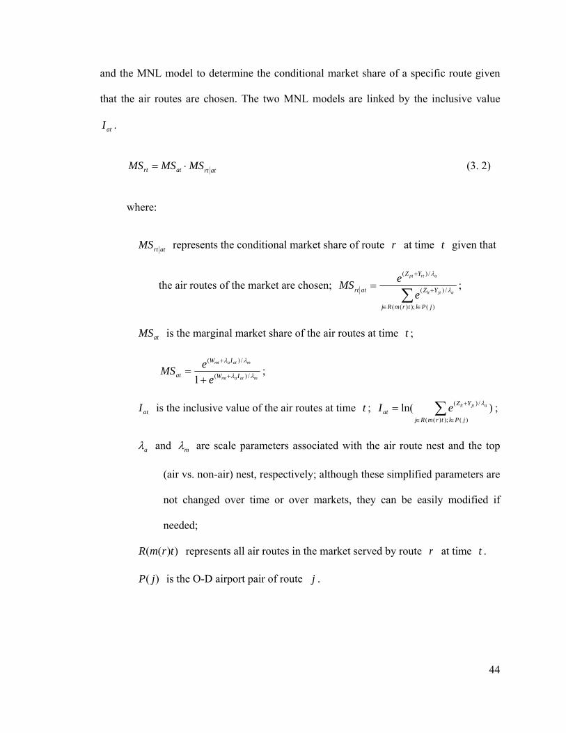
and the MNL model to determine the conditional market share of a specific route given
that the air routes are chosen. The two MNL models are linked by the inclusive value
. atI
atrtatrt MSMSMS ⋅= (3. 2)
where:
atrtMS represents the conditional market share of route r at time t given that
the air routes of the market are chosen; ∑
∈∈
+
+
=
)( );)((mR
e/)jt(
/)(
jPltrj
YZ
YZ
atrt alt
artpt
eMS λ
λ
;
atMS is the marginal market share of the air routes at time ; t
matamt
matamt
IW
IW
at eeMS λλ
λλ
/)(
/)(
1 +
+
+= ;
atI is the inclusive value of the air routes at time ; ; t )ln()( );)((
/)(∑∈∈
+=jPltrmRj
YZat
ajtlteI λ
aλ and mλ are scale parameters associated with the air route nest and the top
(air vs. non-air) nest, respectively; although these simplified parameters are
not changed over time or over markets, they can be easily modified if
needed;
))(( trmR represents all air routes in the market served by route r at time t .
)( jP is the O-D airport pair of route j .
44
The two-level NL model is consistent with utility-maximization for all possible
values of the explanatory variables if 10 ≤<m
a
λλ , where
m
a
λλ is the coefficient of ,
the inclusive value of the air routes at time . Note that either
atI
t aλ or mλ can be
normalized to one. The condition becomes 10 ≤< aλ in the case of normalizing 1=mλ .
In addition, if the hypothesis 1=m
a
λλ cannot be rejected, the two-level NL model
reduces to the MNL model.
Three-Level Nested Logit—A
In addition to differentiating air routes from non-air alternative, the first three-level
nested logit (NL3A, thereafter) further investigates the correlations of connecting routes
with the same O-D airport pair. The nesting structure of the NL3A model is shown in
Figure 3.3. This model implies that (1) direct routes of a market have proportional
substitution patterns, and (2) connecting routes more likely substitute for other
connecting routes within the same O-D airport pair than substitute for other routes (direct
routes and connecting routes of other O-D airport pairs). For example, the connecting
route O1H1D1 more likely substitutes for the connecting route O1H2D1, than for the route
O1D2 or O1H2D2.
45
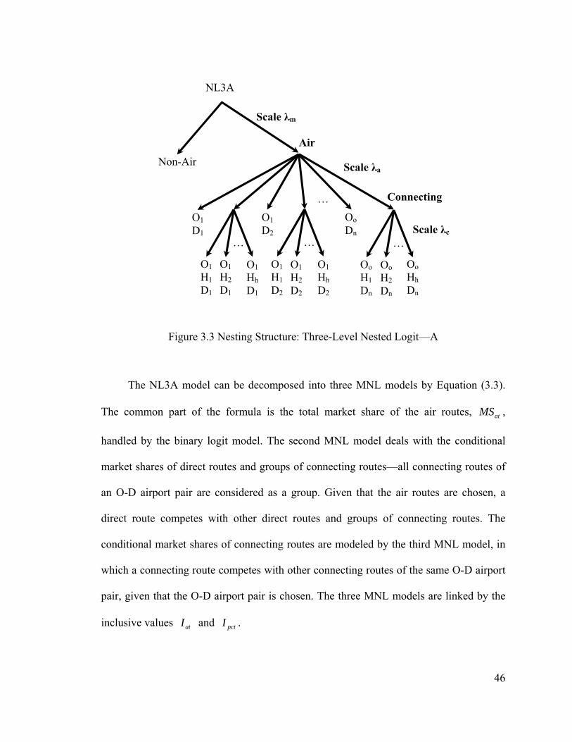
Connecting
Non-Air
Air
Scale λa
Scale λm
O1 D1
O1 D2
O1 H1 D1
O1 H2 D1
O1 H1 D2
O1 H2 D2
O1 Hh D1
O1 Hh D2
…
… Oo Dn
Oo H1 Dn
Oo H2 Dn
Oo Hh Dn
NL3A
… … Scale λc
Figure 3.3 Nesting Structure: Three-Level Nested Logit—A
The NL3A model can be decomposed into three MNL models by Equation (3.3).
The common part of the formula is the total market share of the air routes, ,
handled by the binary logit model. The second MNL model deals with the conditional
market shares of direct routes and groups of connecting routes—all connecting routes of
an O-D airport pair are considered as a group. Given that the air routes are chosen, a
direct route competes with other direct routes and groups of connecting routes. The
conditional market shares of connecting routes are modeled by the third MNL model, in
which a connecting route competes with other connecting routes of the same O-D airport
pair, given that the O-D airport pair is chosen. The three MNL models are linked by the
inclusive values and .
atMS
atI pctI
46
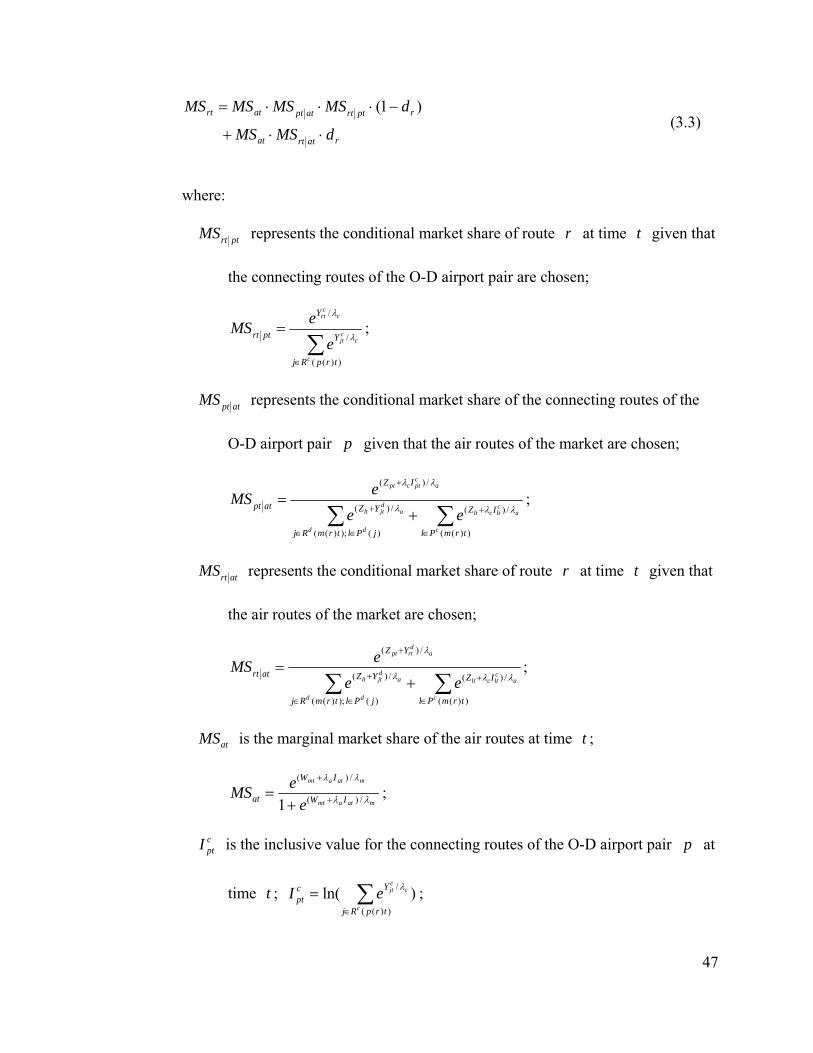
ratrtat
rptrtatptatrt
dMSMS
dMSMSMSMS
⋅⋅+
−⋅⋅⋅= )1( (3.3)
where:
ptrtMS represents the conditional market share of route r at time given that
the connecting routes of the O-D airport pair are chosen;
t
∑∈
=
))((
/
/
trpRj
Y
Y
ptrt
c
ccjt
cc
rt
eeMS
λ
λ
;
atptMS represents the conditional market share of the connecting routes of the
O-D airport pair p given that the air routes of the market are chosen;
∑∑∈ );
(
Plt
e∈
+
∈
+
+
+=
))((
/)(
)()((
/)
/)(
trmPl
IZ
jrmRj
YZ
IZ
atpt
c
acltclt
dd
adjtlt
acptcpt
eeMS
λλλ
λλ
;
atrtMS represents the conditional market share of route r at time t given that
the air routes of the market are chosen;
∑∑∈
+
∈∈
+
+
+=
))((
/)(
)( );)((
/)(
/)(
trmPl
IZ
jPltrmRj
YZ
YZ
atrt
c
acltclt
dd
adjtlt
ad
rtpt
eeeMS
λλλ
λ
;
atMS is the marginal market share of the air routes at time ; t
matamt
matamt
IW
IW
at eeMS λλ
λλ
/)(
/)(
1 +
+
+= ;
cptI is the inclusive value for the connecting routes of the O-D airport pair p at
time ; ; t )ln())((
/∑∈
=trpRj
Ycpt
c
ccjteI λ
47
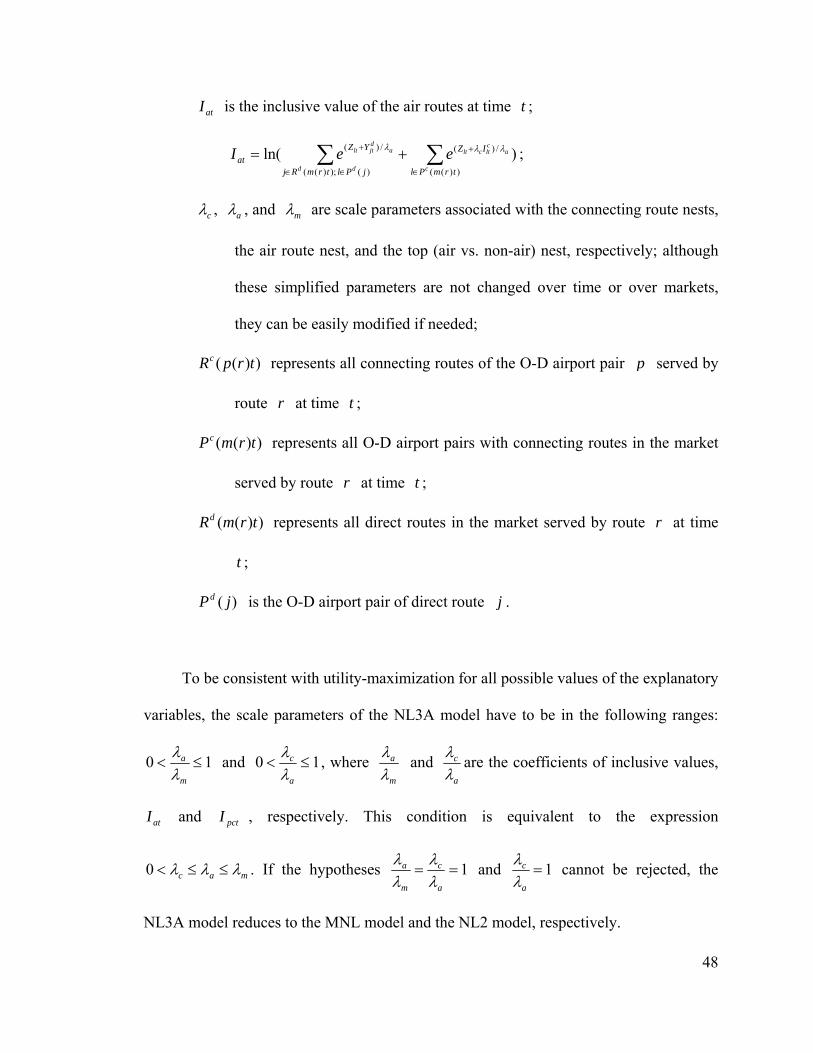
atI is the inclusive value of the air routes at time ;
;
t
)ln())((
/)(
)( );)((
/)( ∑∑∈
+
∈∈
+ +=trmPl
IZ
jPltrmRj
YZat
c
acltclt
dd
adjtlt eeI λλλ
cλ , aλ , and mλ are scale parameters associated with the connecting route nests,
the air route nest, and the top (air vs. non-air) nest, respectively; although
these simplified parameters are not changed over time or over markets,
they can be easily modified if needed;
))(( trpRc represents all connecting routes of the O-D airport pair p served by
route r at time ; t
))(( trmPc represents all O-D airport pairs with connecting routes in the market
served by route r at time t ;
))(( trmRd represents all direct routes in the market served by route r at time
; t
)( jPd is the O-D airport pair of direct route j .
To be consistent with utility-maximization for all possible values of the explanatory
variables, the scale parameters of the NL3A model have to be in the following ranges:
10 ≤<m
a
λλ and 10 ≤<
a
c
λλ , where
m
a
λλ and
a
c
λλ are the coefficients of inclusive values,
and , respectively. This condition is equivalent to the expression atI pctI
mac λλλ ≤≤<0 . If the hypotheses 1==a
c
m
a
λλ
λλ and 1=
a
c
λλ cannot be rejected, the
NL3A model reduces to the MNL model and the NL2 model, respectively.
48
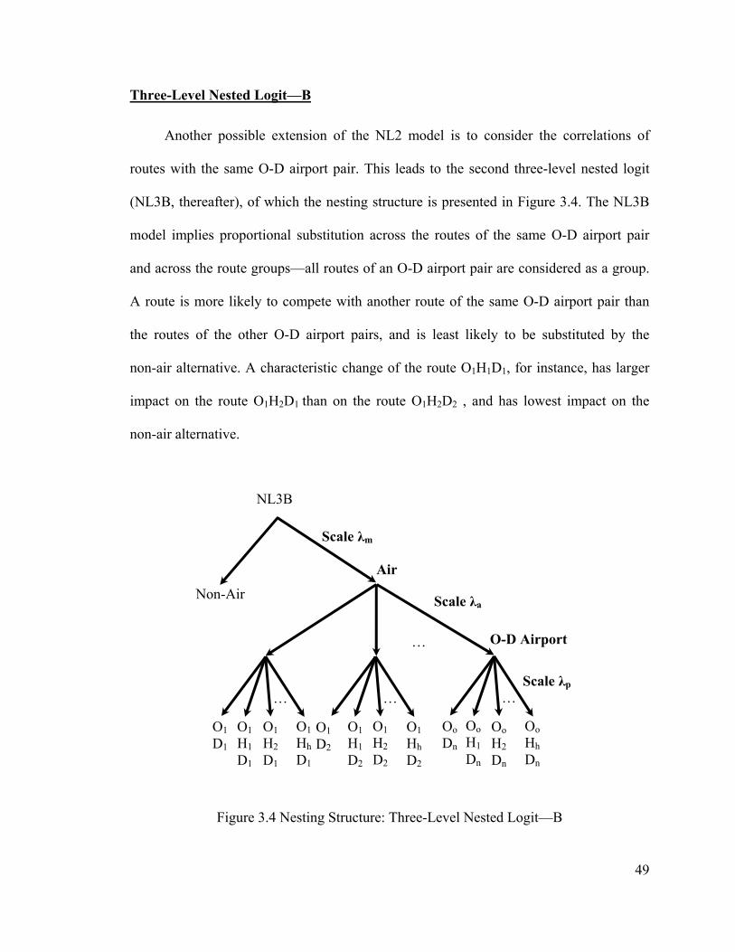
Three-Level Nested Logit—B
Another possible extension of the NL2 model is to consider the correlations of
routes with the same O-D airport pair. This leads to the second three-level nested logit
(NL3B, thereafter), of which the nesting structure is presented in Figure 3.4. The NL3B
model implies proportional substitution across the routes of the same O-D airport pair
and across the route groups—all routes of an O-D airport pair are considered as a group.
A route is more likely to compete with another route of the same O-D airport pair than
the routes of the other O-D airport pairs, and is least likely to be substituted by the
non-air alternative. A characteristic change of the route O1H1D1, for instance, has larger
impact on the route O1H2D1 than on the route O1H2D2 , and has lowest impact on the
non-air alternative.
O-D Airport
Non-Air
Air
Scale λa
Scale λm
O1 D1
O1 D2
O1 H1 D1
O1 H2 D1
O1 H1 D2
O1 H2 D2
O1 Hh D1
O1 Hh D2
…
Oo Dn
Oo H1 Dn
Oo H2 Dn
Oo Hh Dn
NL3B
… Scale λp
……
Figure 3.4 Nesting Structure: Three-Level Nested Logit—B
49
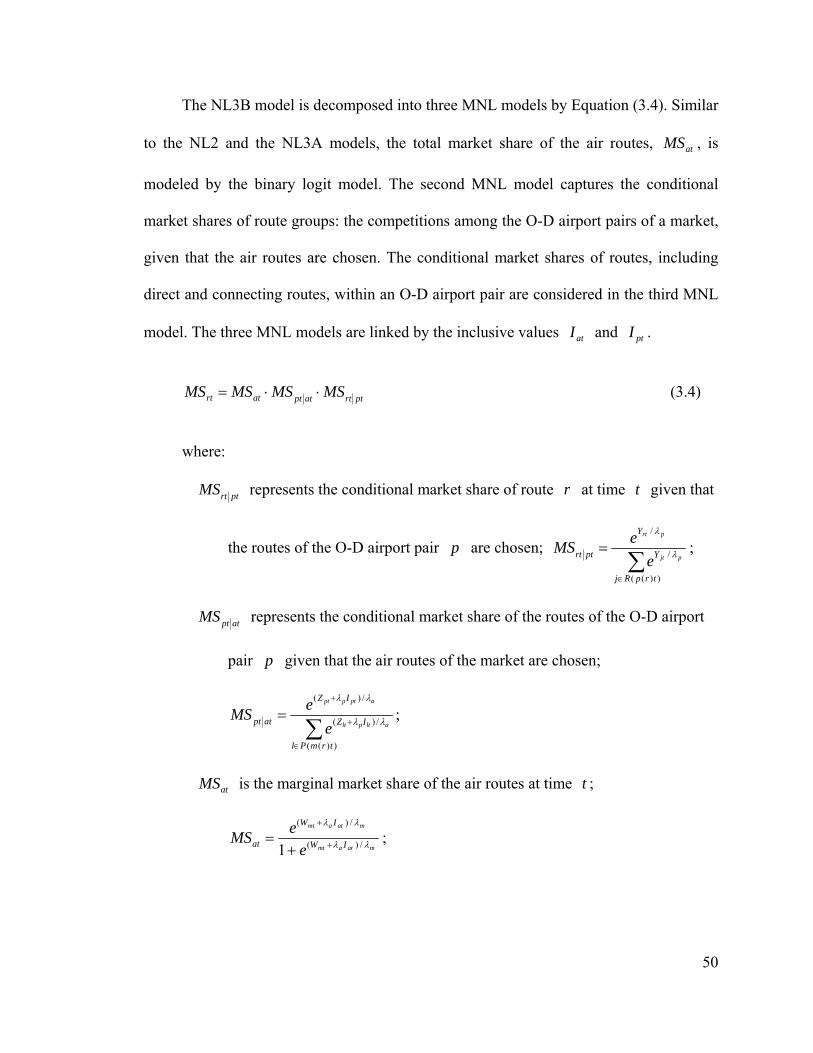
The NL3B model is decomposed into three MNL models by Equation (3.4). Similar
to the NL2 and the NL3A models, the total market share of the air routes, , is
modeled by the binary logit model. The second MNL model captures the conditional
market shares of route groups: the competitions among the O-D airport pairs of a market,
given that the air routes are chosen. The conditional market shares of routes, including
direct and connecting routes, within an O-D airport pair are considered in the third MNL
model. The three MNL models are linked by the inclusive values and .
atMS
atI ptI
ptrtatptatrt MSMSMSMS ⋅⋅= (3.4)
where:
ptrtMS represents the conditional market share of route r at time given that
the routes of the O-D airport pair
t
p are chosen; ∑
(( p
Yrte
∈
=
))
/
/
trRj
Yptrt pjt
p
e λ
λ
MS ;
atptMS represents the conditional market share of the routes of the O-D airport
pair p given that the air routes of the market are chosen;
∑∈
+
+
=
))((
/)(
/)(
trmPl
IZ
IZ
atpt altplt
aptppt
eeMS λλ
λλ
;
atMS is the marginal market share of the air routes at time ; t
matamt
matamt
IW
IW
at eeMS λλ
λλ
/)(
/)(
1 +
+
+= ;
50
ptI is the inclusive value of the O-D airport pair p at time ;
;
t
)ln())((
/∑∈
=trpRj
Ypt
pjteI λ
atI is the inclusive value of the air routes at time ; ; t )ln())((
/)(∑∈
+=trmPl
IZat
altplteI λλ
pλ , aλ , and mλ are scale parameters associated with the O-D airport pair nests,
the air route nest, and the top (air vs. non-air) nest, respectively; although
these simplified parameters are not changed over time or over markets,
they can be easily modified if needed;
))(( trpR represents all routes of the O-D airport pair p served by route r at
time ; t
))(( trmP represents all O-D airport pairs in the market served by route r at
time . t
The NL3B model is consistent with utility-maximization for all possible values of
the explanatory variables if 10 ≤<m
a
λλ and 10 ≤<
a
p
λλ
, where m
a
λλ and
a
p
λλ
are the
coefficients of inclusive values, and , respectively. Note that either atI ptI pλ , aλ , or
mλ can be normalized to one. In the case of normalizing 1=mλ , the condition becomes
1=≤≤ map0 < λλλ . If pλ is chosen to be one, the condition is map λλλ ≤≤=1 . In
addition, the NL3B model reduces to the MNL model and the NL2 model, if the
hypotheses 1==a
p
m
a
λλ
λλ and 1=
a
p
λλ
cannot be rejected, respectively.
51
52
Four-Level Nested Logit
Combining the NL3A and the NL3B models gives the four-level nested logit (NL4,
thereafter), which considers the correlations among the air routes, the O-D airport pairs,
and the connecting routes of an O-D airport pairs. The nesting structure of the NL4 model
is shown in Figure 3.5. This model implies proportional substitution across the
connecting routes of the same O-D airport pair. A connecting route is expected to
substitute, in order from high to low possibilities, for the connecting routes of the same
O-D airport pair, the direct route of the same O-D airport pair, the routes of the other O-D
airport pairs, and the non-air alternative. For example, the impact of a change in the
characteristics of the route O1H1D1 is expected to be successively less on the route
O1H2D1, the direct route O1D1, the route O1H2D2, and the non-air alternative.
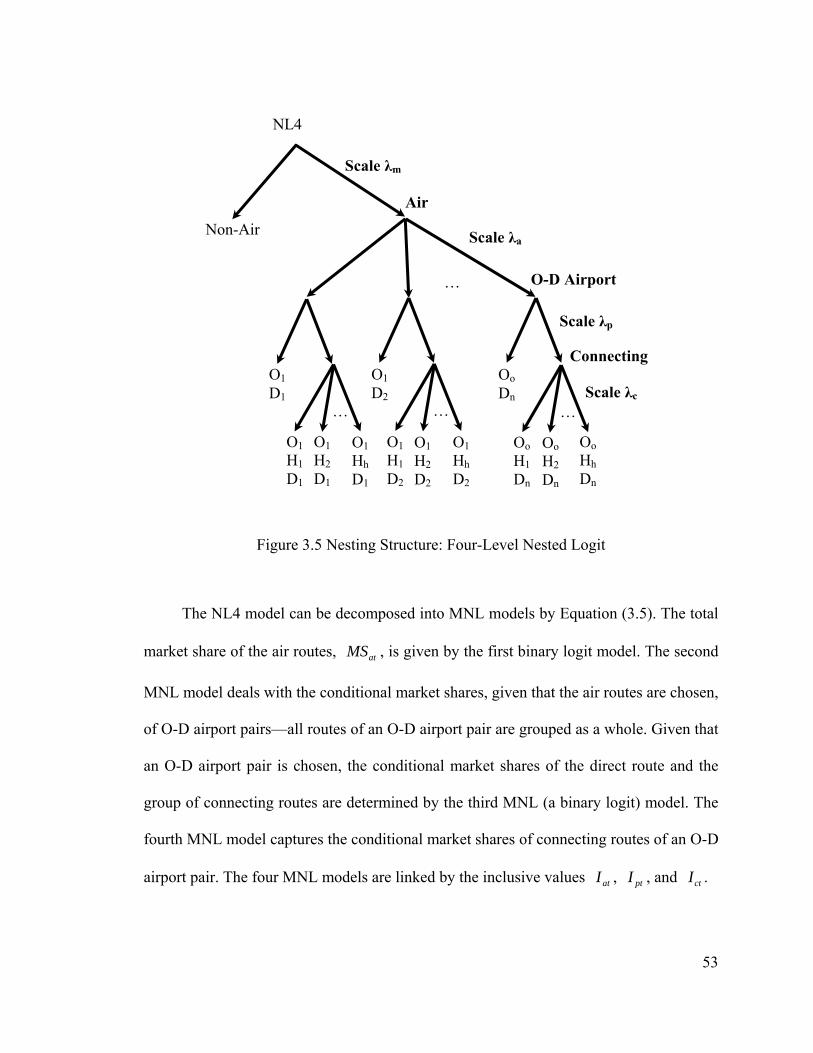
O-D Airport
Non-Air
Air
Scale λa
Scale λm
O1 D1
O1 D2
…
Oo Dn
NL4
Scale λp
O1 H1 D1
O1 H2 D1
O1 H1 D2
O1 H2 D2
O1 Hh D1
O1 Hh D2
…
Oo H1 Dn
Oo H2 Dn
Oo Hh Dn
… …
Connecting
Scale λc
Figure 3.5 Nesting Structure: Four-Level Nested Logit
The NL4 model can be decomposed into MNL models by Equation (3.5). The total
market share of the air routes, , is given by the first binary logit model. The second
MNL model deals with the conditional market shares, given that the air routes are chosen,
of O-D airport pairs—all routes of an O-D airport pair are grouped as a whole. Given that
an O-D airport pair is chosen, the conditional market shares of the direct route and the
group of connecting routes are determined by the third MNL (a binary logit) model. The
fourth MNL model captures the conditional market shares of connecting routes of an O-D
airport pair. The four MNL models are linked by the inclusive values , , and .
atMS
atI ptI ctI
53
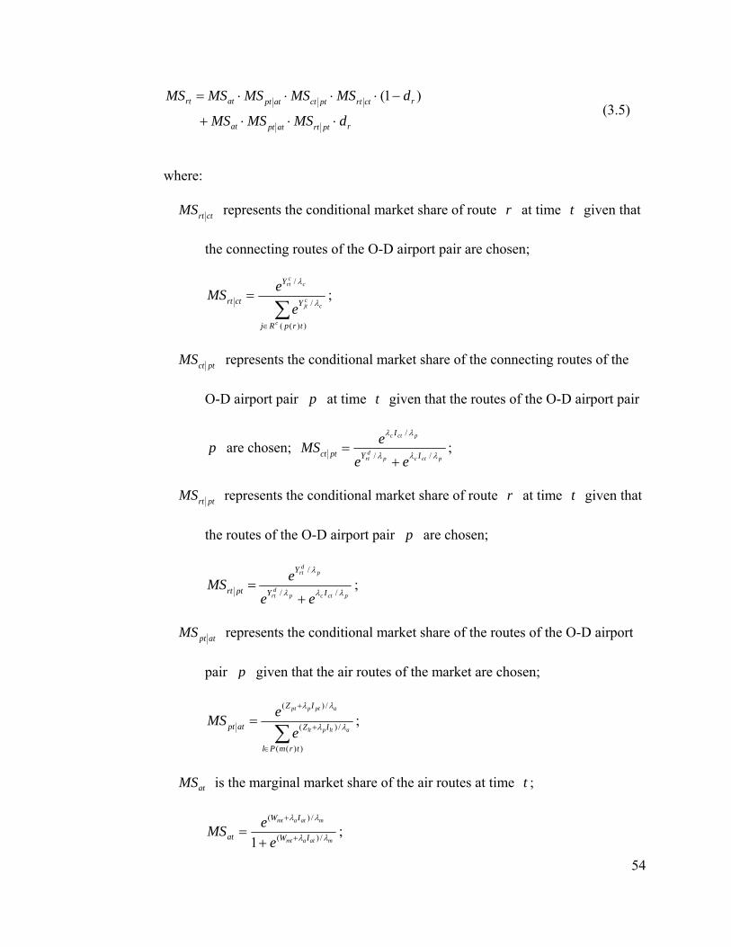
rptrtatptat
rctrtptctatptatrt
dMSMSMS
dMSMSMSMSMS
⋅⋅⋅+
−⋅⋅⋅⋅= )1( (3.5)
where:
ctrtMS represents the conditional market share of route r at time t given that
the connecting routes of the O-D airport pair are chosen;
∑∈
=
))((
/
/
trpRj
Y
Y
ctrt
c
ccjt
cc
rt
eeMS
λ
λ
;
ptctMS represents the conditional market share of the connecting routes of the
O-D airport pair p at time t given that the routes of the O-D airport pair
p are chosen; pctcp
drt
pctc
IY
I
ptctee
eλ/
MSλλ
λλ
/
/
+= ;
ptrtMS represents the conditional market share of route r at time given that
the routes of the O-D airport pair
t
p are chosen;
pctcpd
rt
pd
rt
IY
Y
ptrtee
eMSλλλ
λ
//
/
+= ;
atptMS represents the conditional market share of the routes of the O-D airport
pair p given that the air routes of the market are chosen;
∑∈
+
+
=
))((
/)(
/)(
trmPl
IZ
IZ
atpt altplt
aptppt
eeMS λλ
λλ
;
atMS is the marginal market share of the air routes at time ; t
matamt
matamt
IW
IW
at eeMS λλ
λλ
/)(
/)(
1 +
+
+= ;
54
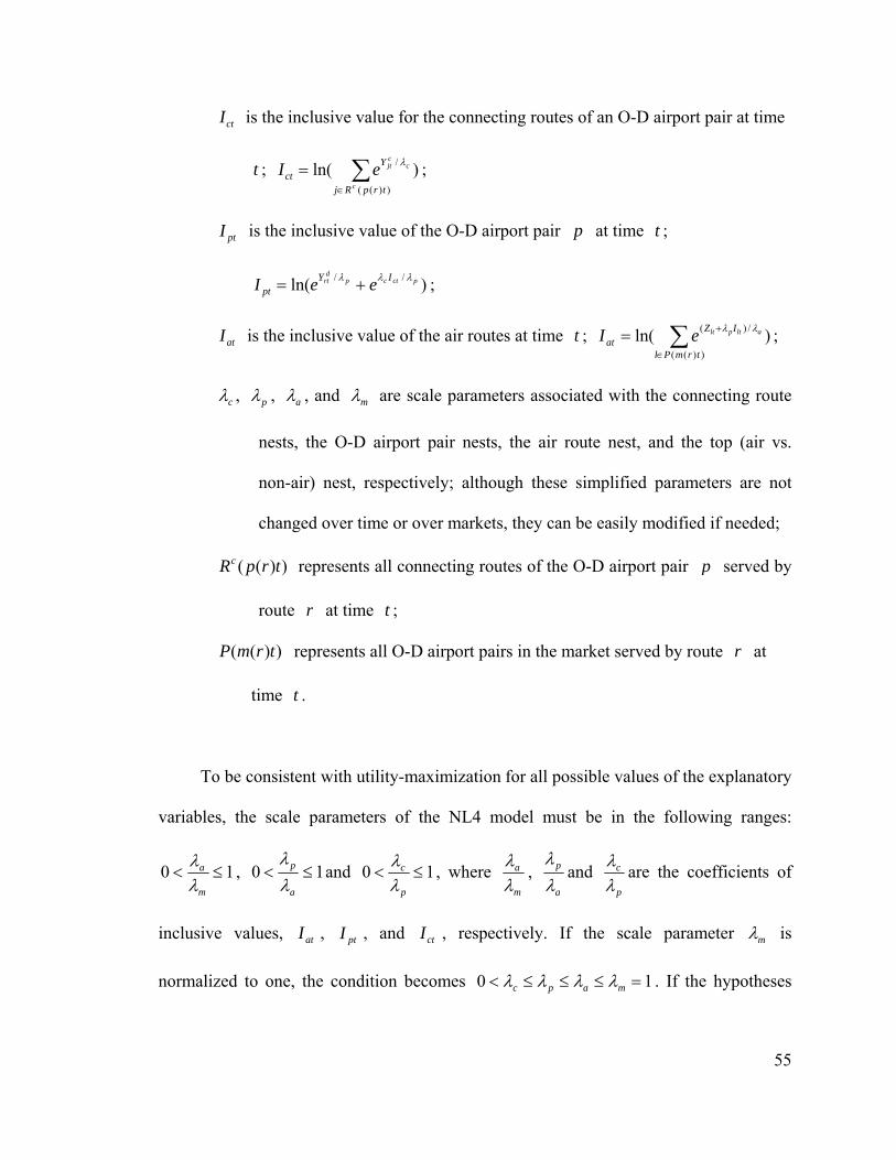
ctI is the inclusive value for the connecting routes of an O-D airport pair at time
; ; t )ln())((
/∑∈
=trpRj
Yct
c
ccjteI λ
ptI is the inclusive value of the O-D airport pair p at time t ;
; )ln( // pctcpd
rt IYpt eeI λλλ +=
atI is the inclusive value of the air routes at time ; ; t )ln())((
/)(∑∈
+=trmPl
IZat
altplteI λλ
cλ , pλ , aλ , and mλ are scale parameters associated with the connecting route
nests, the O-D airport pair nests, the air route nest, and the top (air vs.
non-air) nest, respectively; although these simplified parameters are not
changed over time or over markets, they can be easily modified if needed;
))(( trpRc represents all connecting routes of the O-D airport pair p served by
route r at time ; t
))(( trmP represents all O-D airport pairs in the market served by route r at
time . t
To be consistent with utility-maximization for all possible values of the explanatory
variables, the scale parameters of the NL4 model must be in the following ranges:
10 ≤<m
a
λλ , 10 ≤<
a
p
λλ
and 10 ≤<p
c
λλ , where
m
a
λλ ,
a
p
λλ
and p
c
λλ are the coefficients of
inclusive values, , , and , respectively. If the scale parameter atI ptI ctI mλ is
normalized to one, the condition becomes 10 =≤≤≤< mapc λλλλ . If the hypotheses
55
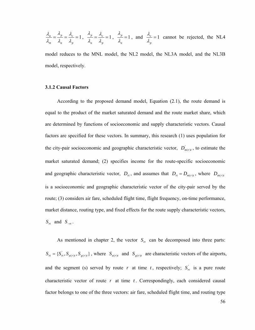
1===p
c
a
p
m
a
λλ
λλ
λλ , 1==
p
c
a
p
λλ
λλ
, 1=a
p
λλ
, and 1=p
c
λλ cannot be rejected, the NL4
model reduces to the MNL model, the NL2 model, the NL3A model, and the NL3B
model, respectively.
3.1.2 Causal Factors
According to the proposed demand model, Equation (2.1), the route demand is
equal to the product of the market saturated demand and the route market share, which
are determined by functions of socioeconomic and supply characteristic vectors. Causal
factors are specified for these vectors. In summary, this research (1) uses population for
the city-pair socioeconomic and geographic characteristic vector, , to estimate the
market saturated demand; (2) specifies income for the route-specific socioeconomic
and geographic characteristic vector, , and assumes that , where
is a socioeconomic and geographic characteristic vector of the city-pair served by the
route; (3) considers air fare, scheduled flight time, flight frequency, on-time performance,
market distance, routing type, and fixed effects for the route supply characteristic vectors,
and .
')( trmD
trmD )(=rtD rtD trmD )(
rtS rtS−
As mentioned in chapter 2, the vector can be decomposed into three parts:
, where and are characteristic vectors of the airports,
and the segment (s) served by route
rtS
tr )},,{ )()('
trgtrartrt SSSS = traS )( gS (
r at time t , respectively; is a pure route
characteristic vector of route
'rtS
r at time . Correspondingly, each considered causal
factor belongs to one of the three vectors: air fare, scheduled flight time, and routing type
t
56
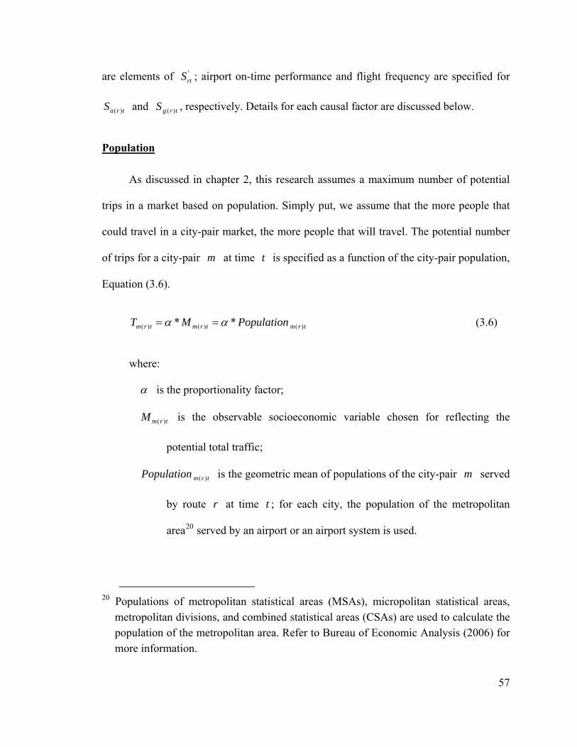
are elements of ; airport on-time performance and flight frequency are specified for
and , respectively. Details for each causal factor are discussed below.
'rtS
traS )( trgS )(
Population
As discussed in chapter 2, this research assumes a maximum number of potential
trips in a market based on population. Simply put, we assume that the more people that
could travel in a city-pair market, the more people that will travel. The potential number
of trips for a city-pair at time t is specified as a function of the city-pair population,
Equation (3.6).
m
trmtrtrm PopulationT )( )()( *mM*α α (3.6) = =
where:
α is the proportionality factor;
trm )(
Population
M is the observable socioeconomic variable chosen for reflecting the
potential total traffic;
m tr )( is the geometric mean of populations of the city-pair served
by route
m
r at time t ; for each city, the population of the metropolitan
area20 served by an airport or an airport system is used.
20 Populations of metropolitan statistical areas (MSAs), micropolitan statistical areas,
metropolitan divisions, and combined statistical areas (CSAs) are used to calculate the population of the metropolitan area. Refer to Bureau of Economic Analysis (2006) for more information.
57
58
The proportionality factor α is set to be 10 when quarter is chosen for the time
frame, i.e. every unit of population may make 10 trips per quarter. Note that 10 is a large
number of potential trips for intercity travel. The real number of air trips is much smaller
than the potential, since air travel costs are high. Sensitivity tests for this setting are
performed to check the robustness of the model parameters.
Although population is not explicitly specified in the market share function, it still
helps to explain—through its impact on the calculation of market shares—the market
share variation between the air routes and the non-air alternative, both across markets and
over time. Refer to Appendix A for details.
Income
Income is used to capture the economic activities that generate air travel demand
and potential travelers’ purchasing power. Both economic activity and purchasing power
are expected to have positive impacts on air travel demand. Thus, higher income level is
expected to generate more air trips. The geometric mean21 of incomes of two cities is
used as an explanatory variable for the city-pair demand. For each city, the income
variable is measured by the per capita personal income (in constant dollars, based on the
4th quarter of 2004) of the metropolitan area served by an airport or an airport system.
Even though the income variable is specified in the market share function, its role
is similar to those income variables in the traditional demand generation models. Because
21 Employing the geometric mean implies that market demand of a city-pair is not
affected by income of one city if the other city has zero income.
59
the income level is the same for all air routes of a market, the income variable does not
affect the relative market shares of different air routes. It, however, explicitly explains the
market share variation between the air routes and the non-air alternative, both across
markets and over time.
Price
According to economic theory, price plays a major role in demand. This is also true
in air travel demand models, although some studies omitted this factor due to data
inavailability or econometric issues, such as the possibility of endogeneity bias. From a
traveler’s perspective, the full price (total monetary costs) of an air alternative may
include the air fare and the access costs—for instance, paying for the transit ticket or
parking fees—for the alternative. Since air fare is usually the dominant component of
these costs, especially for long-haul markets, it is used to capture the effect of price on air
route demand. This variable is measured by the average fare of a route in 2004 (the 4th
quarter) constant dollars.
As mentioned in section 2.1.3, the air fare variable may be endogenous, because of
supply and demand simultaneity and/or omitted variables. As a result, the coefficients
estimated by ordinary least squares (OLS) method may be biased. In air travel demand
models, the fare coefficient is more likely biased towards zero22. Thus, the inferred fare
22 Because airlines may set fares based on some demand side variables—such as traffic flow, demand estimations ignoring simultaneity of supply and demand systems may give results that travelers seem to prefer higher air fares. In addition, higher fares may be due to better services. If a model does not take an important service characteristic into account, the estimated fare coefficient may be affected by the fact that passengers
60
elasticities and the value-of-time may be underestimated and overestimated, respectively.
This research applies the instrumental variables (IV) estimation, in which a cost side
variable23 is chosen as the instrument for air fare, to solve the endogeneity problem.
Although the access costs may also affect travelers’ decisions on routes,
particularly for the airport choice in multiple airport systems, this research does not
explicitly specify the access cost variables in the model mainly due to the data
availability. Totally omitting the access cost variables may affect the estimated
coefficients of other specified variables if (1) the impacts of access cost on route choice is
substantial, and (2) the omitted and specified variables are correlated. For example, a
route starting from an airport closer to a city center may have higher air fare than a route
starting from an airport far from the city center, all other factors being equal. If this is the
case, air fare is negatively correlated with access costs. Since access costs are expected to
have negative impacts on demand, the estimated coefficient of air fare is expected to be
biased24 towards zero, if the model excludes access cost. In this research, the effects of
access costs are implicitly captured by the fixed effect dummy variables, such as time and
(origin and destination) airport dummy variables. In addition, applying the IV to air fare
should eliminate the impact on the fare coefficient from omitting access cost variables.
prefer better services (measured by the characteristic). Therefore, both simultaneity and omitted variables may lead the estimated coefficients that are biased upward.
23 More specifically, the cost variable is defined as the product of the route distance and unit jet fuel cost. See section 3.3 Model Estimation for more details.
24 Refer to Wooldridge (2003) or other econometrics textbooks for general expressions.
61
Scheduled Flight Time
In addition to money, potential travelers also spend time on travel. Total travel time
of a trip—from the origin to the destination—should be used to capture the time effect,
which is expected to be negative: on average, travelers would prefer shorter travel time.
The total travel time is mainly composed of access time, scheduled flight time, schedule
delay, connecting time (if any), and flight delay. Figure 3.6 describes these time
components, except for access time. The deterministic and stochastic parts of the total
travel time are shown in solid and dashed lines, respectively. Note that arrival delay at a
connecting airport, if huge enough, may cause missed connections and schedule changes
for travelers. In addition, because these time components may have different marginal
effects 25 , analyzing the time effect by its components allows for more flexibility.
Scheduled flight time is discussed in this sub-section, and other time components are
analyzed in the following sub-sections.
25 For example, one hour of arrival delay may be much worse than one hour of scheduled
flight time. A passenger may miss her or his connecting flight due to the arrival delay, while he or she can plan in advance for the longer scheduled flight time.
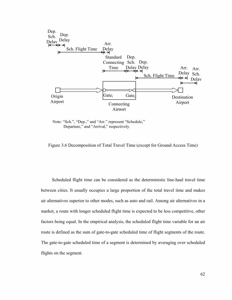
Dep. Sch.
Delay Dep. Delay
Arr. Delay
Arr. Delay
Dep. Delay
Dep. Sch.
Delay
Standard Connecting
Time Arr. Sch.
Delay
Sch. Flight Time
Sch. Flight Time
Origin Airport
Destination Airport Connecting
Airport
Gatei Gatej
Note: “Sch.”, “Dep.,” and “Arr.” represent “Schedule,” Departure,” and “Arrival,” respectively.
Figure 3.6 Decomposition of Total Travel Time (except for Ground Access Time)
Scheduled flight time can be considered as the deterministic line-haul travel time
between cities. It usually occupies a large proportion of the total travel time and makes
air alternatives superior to other modes, such as auto and rail. Among air alternatives in a
market, a route with longer scheduled flight time is expected to be less competitive, other
factors being equal. In the empirical analysis, the scheduled flight time variable for an air
route is defined as the sum of gate-to-gate scheduled time of flight segments of the route.
The gate-to-gate scheduled time of a segment is determined by averaging over scheduled
flights on the segment.
62
63
Airlines may add buffer time into schedules to improve on-time performance26.
This may affect the estimated effects of scheduled flight time and on-time performance.
The scheduled flight time that includes buffer time is not only associated with route
distance but also with delay which is measured against schedule. The estimated results of
scheduled flight time and delay need to be explained carefully. For example, when
evaluating delay impacts, a researcher should note that the estimates based only on delay
variables may be inaccurate, because parts of the delay impacts are absorbed by
scheduled flight time. The bottom line is that scheduled flight time and delay capture the
effect of buffer time, although they should be explained with caution.
Flight Frequency
The greater the number of flights, the more convenient traveling between two cities
is. From the viewpoint of travel time, higher flight frequency generally causes shorter
schedule delay, which refers to the time difference between desired and actual schedule
arrival/ departure times, and thus shorter planed total travel time. In addition, higher
frequency is more likely to keep a traveler close to his or her original schedule when
unexpected events, such as flight cancellations and delays, happen. For instance, a
traveler missing a flight on a high-frequency segment may only wait for one hour for
26 If the marginal effect of delay is greater than that of scheduled flight time, shifting the
same unit of time (e.g. 10 minutes) from delay to scheduled flight time makes an air route more attractive. However, adding buffer time may cost more than it may gain, since it reduces aircraft utilization. The trade-off between on-time performance and aircraft utilization limits the length of buffer time.
64
another flight, while the same situation on a low-frequency segment may cost him or her
one night.
Flight frequency may affect a potential traveler’s decision by changing his or her
choice set, especially when flight searching costs are high for the traveler. Higher
frequency routes are more likely to be included in travelers’ choice sets, and thus to be
chosen. For example, when a potential traveler books his or her flight through a travel
agent, the agent may only provides a few number of alternatives to the potential traveler,
based on the potential traveler’s desired departure or arrival time. Low frequency routes
may not be suggested to the potential traveler because they are a little out of the desired
time window, even though they may have better attributes such as lower fares. Another
example27 is that a potential traveler may first call an airline that provides more—at least
he or she believes so—flights in the O-D market. The potential traveler may pick one of
the offered alternatives from this airline if he or she feels it is satisfactory. In both cases,
the potential travelers may not search for other travel agents or airlines, because of flight
search costs.
As suggested by Hansen (1990), flight frequency is taken in logarithmic form for
two reasons. First, marginal effects of flight frequency on route utilities are expected to
be diminishing with increasing number of flights. Second, a route alternative can be
considered as an aggregation of detailed alternatives, and frequency is a measure of the
27 This is an example of airline choice, rather than route choice. However, in practice,
choosing a route may be equivalent to choosing an airline, because the connecting airport of a route is dominated by a specific airline.
65
size of the route alternative. The logarithmic form is the most suitable 28 for a
characteristic that captures the size of an aggregated alternative.
Since flight frequency is a segment characteristic, a route utility function may
include several frequency variables. This research specifies three frequency variables—
one for direct routes and two29 for connecting routes, and expects their marginal effects
are different. In particular, this research differentiates the frequency effects for
connecting routes by taking maximal and minimal numbers of flights on two segments.
The hypothesis is that the minimum frequency is more critical to the connecting service,
and thus a given fractional flight frequency increase on the segment with lower frequency
should increase service attractiveness more than an equivalent change on the segment
with higher frequency.
Note that it is possible that observed flight frequency is endogenous, because of
supply and demand simultaneity—airlines would schedule more flights if they think there
will be high demand on a segment; potential travelers prefer high frequency routes as
described above. As a result, the coefficients estimated by OLS method may be biased.
However, flight frequency is a segment characteristic and each segment may serve many
routes and markets; that is, flight frequency is not solely determined by specific route
traffic. Therefore, the endogeneity bias caused by frequency may not be severe since the
28 Refer to Ben-Akiva and Lerman (1985) for more details. 29 This research discards routes with three or more segments, which carry about 5
percent of passengers, to simplify the analysis. Thus, every connecting route has two segments.
66
proposed model is a route demand model. In addition, the possibility of bias caused by
the frequency endogeneity is less than that resulting from endogeneity of air fare, which
is a route specific characteristic. This research, hence, only focuses on the remedy for
bias caused by the air fare variable.
On-Time Performance
While scheduled flight time and schedule delay (represented by frequency) capture
deterministic parts of total travel time, on-time performance is stochastic in nature.
Whereas travelers accept most characteristics of the service (e.g. fare and scheduled
travel time) before their trips, on-time performance is realized during the trip, and thus
becomes an important determinant of travelers’ ultimate satisfaction30. Better on-time
performance may thereby attract more traffic to the route in the future.
There are many ways to measure on-time performance of a route. Percentage of
on-time (or delayed) flights and average delay per flight are two main categories of these
metrics. The former metric is determined by setting up a threshold, such as 15 minutes: if
a flight arrival or departure delay against schedule is greater than the threshold, it is
counted as a delayed flight. The later metric is equal to the total delay time31 divided by
30 For example, Ross and Swain (2007) argued that “industry surveys consistently
identify departure punctuality as a key determinant of consumer satisfaction, especially on shorter flights.”
31 One may calculate the total delay time by summing the time differences between actual and schedule time for all flights, or for all delayed flights, defined by a delay threshold. This research chooses the first approach. In addition, this research also calculates average positive and negative delays by separating early and late flights.
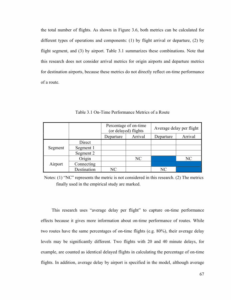
67
the total number of flights. As shown in Figure 3.6, both metrics can be calculated for
different types of operations and components: (1) by flight arrival or departure, (2) by
flight segment, and (3) by airport. Table 3.1 summarizes these combinations. Note that
this research does not consider arrival metrics for origin airports and departure metrics
for destination airports, because these metrics do not directly reflect on-time performance
of a route.
Table 3.1 On-Time Performance Metrics of a Route
Percentage of on-time
(or delayed) flights Average delay per flight
Departure Arrival Departure Arrival
Segment Direct
Segment 1 Segment 2
Airport Origin NC NC
Connecting Destination NC NC
Notes: (1) “NC” represents the metric is not considered in this research. (2) The metrics finally used in the empirical study are marked.
This research uses “average delay per flight” to capture on-time performance
effects because it gives more information about on-time performance of routes. While
two routes have the same percentages of on-time flights (e.g. 80%), their average delay
levels may be significantly different. Two flights with 20 and 40 minute delays, for
example, are counted as identical delayed flights in calculating the percentage of on-time
flights. In addition, average delay by airport is specified in the model, although average
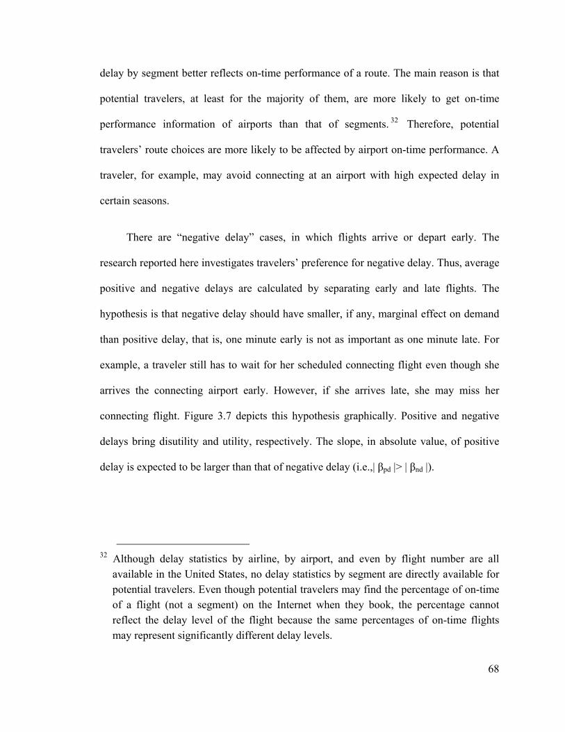
68
delay by segment better reflects on-time performance of a route. The main reason is that
potential travelers, at least for the majority of them, are more likely to get on-time
performance information of airports than that of segments. 32 Therefore, potential
travelers’ route choices are more likely to be affected by airport on-time performance. A
traveler, for example, may avoid connecting at an airport with high expected delay in
certain seasons.
There are “negative delay” cases, in which flights arrive or depart early. The
research reported here investigates travelers’ preference for negative delay. Thus, average
positive and negative delays are calculated by separating early and late flights. The
hypothesis is that negative delay should have smaller, if any, marginal effect on demand
than positive delay, that is, one minute early is not as important as one minute late. For
example, a traveler still has to wait for her scheduled connecting flight even though she
arrives the connecting airport early. However, if she arrives late, she may miss her
connecting flight. Figure 3.7 depicts this hypothesis graphically. Positive and negative
delays bring disutility and utility, respectively. The slope, in absolute value, of positive
delay is expected to be larger than that of negative delay (i.e.,| βpd |> | βnd |).
32 Although delay statistics by airline, by airport, and even by flight number are all
available in the United States, no delay statistics by segment are directly available for potential travelers. Even though potential travelers may find the percentage of on-time of a flight (not a segment) on the Internet when they book, the percentage cannot reflect the delay level of the flight because the same percentages of on-time flights may represent significantly different delay levels.
Delay
Utility
0
βpd
βnd
Figure 3.7 Delay and Utility
Since potential travelers do not know their flight delays when they choose their
routes, they may consider expected flight delay as one of the service characteristics. This
research uses flight delays of previous period(s) to capture the expectation. That is, a
potential traveler may prefer a route because he or she knows (e.g. from their experiences
or friends’, or from the Internet) that the airports it includes have good records of on-time
performance. More precisely, the hypothesis is that potential travelers make decisions
based on recent—defined as one and four seasons (subscripted as t-1 and t-4, respectively)
before the decision season (subscripted as t)—available information on on-time
performance. Potential travelers may have impressions of how good or bad the
alternatives are based on recent experience. The delay variable for one quarter before the
decision quarter (t-1) is used to capture this expectation. In addition, the on-time
69
70
performance of aviation systems heavily depends on weather conditions, and thus follows
seasonal patterns. The delay variable for four quarters before the decision quarter (t-4) is
used to account for the seasonal effect.
Routing Type
The more connections required by a route, the lower its convenience. Thus,
potential travelers usually prefer direct routes over connecting routes, all else equal.
Although travelers’ disutility may non-linearly increase with the number of connections,
this research, since it considers only direct and one-connection routes, employs a dummy
variable to capture connection utility. The specified dummy variable captures the fixed
route effects which are not captured by other variables (e.g. fare, scheduled flight time,
and delay). For instance, combined with connecting airport dummy variables, it captures
connecting time.
Market Distance
Market distance may affect potential travelers in two ways: mode choice and
propensity to travel. Since the model includes a non-air alternative, mode competition
should be taken into account in order to estimate the total market share of air routes in a
market. Potential travelers are more likely to choose air service in long-haul markets than
in short-haul markets, as alternative modes—such as automobile and train—are not
available or not competitive in long-haul markets. Considering mode competition effect
only, the total market share of air routes is expected to increase with market distance.
This effect diminishes at larger distances as alternative modes become uncompetitive.
71
That is, the market distance effect due to mode competition may become essentially
constant once as market distance reaches a certain value.
While mode competition concerns the air transport share of the travel market,
distance also effects the overall size of that market. As suggested by the literature on
transportation geography, interactions between distant cities are likely to be fewer. Thus,
propensity to travel induced from such interactions is expected to decrease as distance
increases. Travel costs, including monetary and time costs, may be the main reasons for
this tendency, but factors other than costs are also at play.
As discussed above the effects of distance on mode competition and propensity to
travel may offset each other. The net effect of market distance, thus, may depend on data
and model specification. For example, a study with more long-haul markets in the sample
may find a negative distance effect on demand if a linear relation is specified. Including
fare and travel time as explanatory variables affects the distance coefficient estimate
because of multicollinearity between distance and these variables.
In the air travel demand literature, the majority of studies suggest that distance
prevents people from traveling, mainly due to travel costs increasing with distance. For
instance, De Vany and Garges (1972) find that market distance is negatively correlated
with city-pair air trips. Relatively few studies take mode competition into account when
they investigate distance effects. However, some studies implicitly treat this issue by
estimating different models for different market distance ranges. Corsi, Dresner and
72
Windle (1997) argue that the sign of distance coefficient is indeterminate33 . Their
estimate shows a positive correlation between market distance and city-pair air traffic,
implying that mode competition is the dominant effect. Due to their specification the
relationship, however, is fixed across city-pairs—regardless of service attributes and
distance ranges.
In this research, the net effect of market distance is expected to be positive—it is
more likely dominated by mode competition. The influence of propensity to travel is
weaker since travel cost variables, such as fare and scheduled flight time, are also
included in the model. By the same token, the effect is likely to be concave in distance,
and perhaps decreasing at long distance. As visualized in Figure 3.8, while the marginal
effect of mode competition in shorter-haul markets is strong, it becomes negligible in
longer-haul markets. The influence of propensity to travel may thus prevail in longer-haul
markets.
33 Their justifications are as follows. “On one hand, one would expect more travel
between cities that are relatively close (in distance) to each other; that is distance to be negatively correlated with passenger traffic. On the other hand, closer destinations have the greatest competition from automobiles and trains so that it might be that air passenger traffic increases with route distance.”
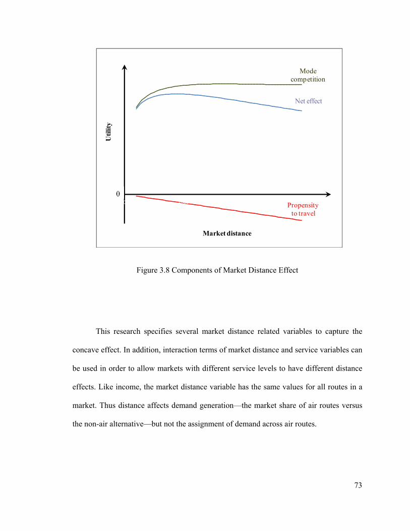
Mode competition
Net effect
pen
-2
9
0 500 1000 1500 2000 2500 3000 3500
Util
ity
Market distance
73
Pro sityto travel
Figure 3.8 Components of Market Distance Effect
This research specifies several market distance related variables to capture the
concave effect. In addition, interaction terms of market distance and service variables can
be used in order to allow markets with different service levels to have different distance
effects. Like income, the market distance variable has the same values for all routes in a
market. Thus distance affects demand generation—the market share of air routes versus
the non-air alternative—but not the assignment of demand across air routes.
74
Other Factors
In addition to the above causal factors, this research specifies several sets of
dummy variables to capture unobserved fixed effects, such as specific airport and time
period effects. The first set of dummy variables is for connecting (hub) airports, since
each connecting airport may have specific conditions that affect potential travelers’
connecting choices that have not been captured by other explanatory variables. For
example, although standard connecting times of hubs are not specified in the model, these
dummy variables could capture such effects if they do not vary much over the time span
of the sample. Twenty-nine dummy variables are used—one for each of the 30
benchmark airports34, except for Tampa International Airport (TPA) which is used as the
benchmark airport.
Another set of dummy variables captures fixed effects of origin and destination
airports. They are only specified for airports in multiple airport systems because potential
travelers do not have a chance to choose among terminal airports in single airport systems.
The functions of the origin and destination airport dummy variables are similar to dummy
variables for connecting airports, but represent different effects. This set of dummy
variables may capture, for instance, differences in airport accessibility.
The third set of dummy variables captures seasonal and yearly fixed effects. Three
and eight dummy variables are used for quarter and year, respectively. People may be
34 To simplify the empirical work, this research only includes direct routes and routes
connecting at one of the 30 benchmark airports in the sample. Refer to section 3.2 for details.
75
more (or less) likely to travel in certain seasons or years, for reasons not captured by
socioeconomic variables in our model. For example, after 9/11, people curtailed air travel
because of security concerns as well as the increased hassle of more stringent screening.
Although this research does not explicitly specify dummy variables for market
fixed effects, the used estimation method (difference-in-differences) implicitly takes
these effects into account by segregating these variables from the utility functions. In our
estimation35, differences of explanatory variables are actually used as regressors to
explain the market share difference between two routes. Since these routes serve the same
market, they have no difference in market fixed effect. Therefore, dummy variables for
market fixed effects are eliminated from the utility functions.
3.2 Data
To estimate the model, this research compiles a panel data set which includes
variables for major U.S. domestic routes over 40 quarters—all quarters between year
1995 and 2004. The raw data is from five sources: (1) DOT’s Airline Origin and
Destination Survey (DB1B); (2) DOT’s T-100; (3) FAA’s Airline Service Quality
Performance System (ASQP); (4) Bureau of Economic Analysis’s Regional Economic
Information System; and (5) Air Transport Association’s Fuel Cost and Consumption
Report. In order to simplify the empirical work and/or get reliable data, the data is filtered
by several rules. In addition, it is necessary to associate airports with metropolitan
regions since the model predicts travel between regions rather than specific airports.
35 Refer to section 3.3 for more information.

76
Data Sources
Information about air passenger itineraries—including fares and routes (origin,
connecting, and destination airports)—is originally from U.S. DOT’s Airline Origin and
Destination Survey (DB1B), which is a 10% sample of airline tickets from reporting
carriers36. Due to data reliability problems, this research does not use raw data from
DB1B. Instead, the used data is extracted from Hub, a commercial product, which cleans
the raw data by comparing different data sources (Data Base Products, 2004a; 2005a).
After filtering (refer to the “Data Filters” sub-section below), average fare and number of
passengers for each route are calculated. In addition, market distances are also provided
by Hub.
Flight frequency data is originally from U.S. DOT’s T-100 database, which
provides U.S. domestic non-stop segment information. This research extracts the data
from Onboard Domestic, also a commercial product of Data Base Products (2004b and
2005b). With flight frequency for all segments in the system, frequency variables for
routes can be determined.
Scheduled flight time and on-time performance variables, including all on-time
performance metrics listed in Table 3.1, are calculated from FAA’s Airline Service
Quality Performance (ASQP) database, which provides actual and scheduled time by
36 According to Data Base Products (2007), these carriers are “all U.S. certificated route
air carriers, except for a) helicopter carriers, b) intra-Alaska carriers, and c) domestic carriers who have been granted waivers because they operate only small aircraft with 60 or fewer seats.”
77
flight by gate departure and gate arrival from reporting carriers 37 . After filtering,
scheduled flight time for each segment in each quarter is computed by averaging
scheduled flight time of all flights on the segment in that quarter. Scheduled flight time
for all routes, then, can be determined. For each airport, average positive and negative
arrival delays are calculated by differentiating flights that arrive before and after their
scheduled time.
Income and population by metropolitan38 information is downloaded from the
Regional Economic Information System, U.S. Bureau of Economic Analysis (2006).
Each origin or destination city is linked to one metropolitan area. Then, the geometric
mean of income or population for each city-pair can be determined. Note that income and
population data is not available for some quarters of a year. In such cases, linear
interpolation is used to estimate these variables.
Unit jet fuel cost39 of U.S. domestic operations is calculated from Air Transport
Association’s Fuel Cost and Consumption Report (2005). Monthly fuel cost and
consumption are summed into quarterly total fuel cost and consumption. Then, for each
37 According to Federal Aviation Administration (2007a), “The Airline Service Quality
Performance System (ASQP) contains data provided by the airlines by flight for airlines that carry at least 1% of all domestic passengers. The number of airlines providing data has varied from 10 to 20.”
38 The metropolitan here includes all metropolitan areas: metropolitan statistical areas (MSAs), micropolitan statistical areas, metropolitan divisions, and combined statistical areas (CSAs). Refer to Bureau of Economic Analysis (2006) for more information.
39 The unit cost (cents per gallon, in 2004 dollars) is used to calculate the instrumental variable, which is defined as the product of the route distance and unit jet fuel cost, for air fare.
78
quarter, the unit jet fuel cost is equal to the total fuel cost divided by the total fuel
consumption.
Data Filters
The data used for estimating the model is filtered, in order to simplify the empirical
work and ensure reliable data. Data filters are as follows.
• This research uses US domestic itineraries with non-zero fares and with one or two
coupons. These itineraries account for about 95% of all US domestic itineraries.
Itineraries served exclusively by commuter carriers are discarded since commuter
carriers did not completely report their activities to DB1B.
• Only itineraries between top 100 origin and destination airports are included in the
sample. The ranking is based on fourth quarter 2004 passenger traffic, excluding
connections. As shown in Figure 3.9, the top 100 airports account for about 95% of
total airport traffic, while maintaining a reasonable computational burden.
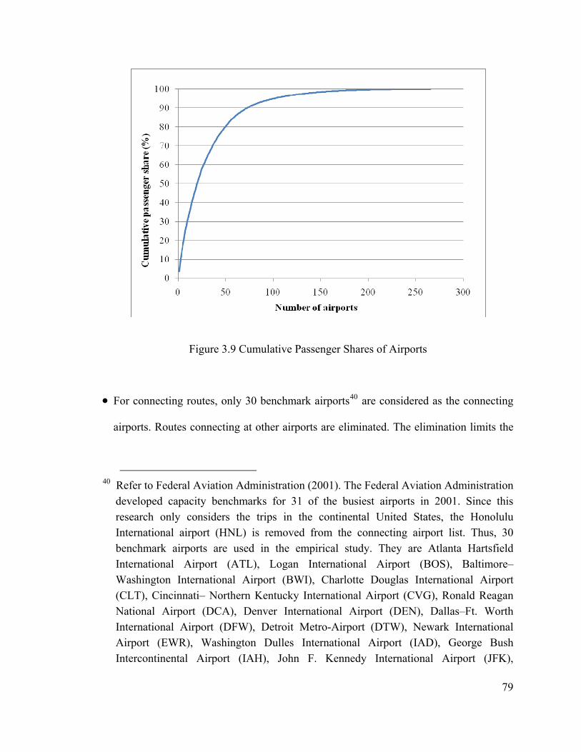
Figure 3.9 Cumulative Passenger Shares of Airports
• For connecting routes, only 30 benchmark airports40 are considered as the connecting
airports. Routes connecting at other airports are eliminated. The elimination limits the
40 Refer to Federal Aviation Administration (2001). The Federal Aviation Administration developed capacity benchmarks for 31 of the busiest airports in 2001. Since this research only considers the trips in the continental United States, the Honolulu International airport (HNL) is removed from the connecting airport list. Thus, 30 benchmark airports are used in the empirical study. They are Atlanta Hartsfield International Airport (ATL), Logan International Airport (BOS), Baltimore– Washington International Airport (BWI), Charlotte Douglas International Airport (CLT), Cincinnati– Northern Kentucky International Airport (CVG), Ronald Reagan National Airport (DCA), Denver International Airport (DEN), Dallas–Ft. Worth International Airport (DFW), Detroit Metro-Airport (DTW), Newark International Airport (EWR), Washington Dulles International Airport (IAD), George Bush Intercontinental Airport (IAH), John F. Kennedy International Airport (JFK),
79
80
number of routes of an O-D airport pair to 31 (one direct route and 30 connecting
routes), which makes the model more tractable with little lose of generality, since the
vast majority of connections occur at the 30 benchmark airports.
• Some routes are discarded because of their unreasonable average yields or low
frequency. This research picks routes with average yields equal or greater than four
cents per mile.41 A minimum of 60 flights per quarter is used to define a normal
scheduled service. Segments and routes with flight frequency less than 60 flights per
quarter are not included in the sample.
• When this research summarizes flight frequency variables from T100 database, flights
served by small aircrafts (fewer than 60 seats) are not incorporated because of data
availability and consistency issues. Prior to October 2002, the T-100 database only
includes the carriers that operate at least one aircraft with more than 60 seats. The data
before the fourth quarter of 2002 for aircraft with fewer than 60 seats are not
representative and thus they are not used. Although all carriers report to T-100
McCarran International Airport (LAS), Los Angeles International Airport (LAX), LaGuardia Airport (LGA), Orlando International Airport (MCO), Memphis International Airport (MEM), Miami International Airport (MIA), Minneapolis–St. Paul International Airport (MSP), Chicago O’Hare International Airport (ORD), Philadelphia International Airport (PHL), Phoenix International Airport (PHX), Pittsburgh International Airport (PIT), San Diego International Airport (SAN), Seattle–Tacoma International Airport (SEA), San Francisco International Airport (SFO), Salt Lake City International Airport (SLC), Lambert–St. Louis International Airport (STL), and Tampa International Airport ( TPA).
41 About 0.8% of routes are discarded by this rule.
81
database after that quarter, this research still removes those flights to keep the data
consistent over time.
• While calculating on-time performance from ASQP database, some flights are not
included because their records are considered to be outliers. Flights with airborne time
shorter than 15 minutes or with arrival delay longer than six hours are discarded. In
addition, for each included flight, the absolute difference between actual and scheduled
airborne time should not be greater than three hours. Additionally, some routes are
automatically removed during model estimation if required delay variables values are
unavailable.
Multiple Airport Systems
While some guidelines exist in the literature, there is no absolute definition of a
multiple airport system (MAS) because each study has a different goal. In order to
implement the model, this research follows the definition of a MAS proposed by Hansen
and Weidner (1995). They defined a MAS using two criteria:42 airports operating in a
metropolitan area and existing competition for local passengers. However, some airports
42 More specifically, Hansen and Weidner (1995) defined “a MAS as consisting of two
or more airports with scheduled passenger enplanements, and which satisfy both of the following criteria: (1) Each airport is included in the same community by the FAA or within 30 miles of the primary airport of an FAA-designated large hub community, or each airport is in the same MSA (Metropolitan Statistical Area) or CMSA (Consolidated Metropolitan Statistical Area); (2) The Herfindahl concentration index for airports is less than 0.95.”
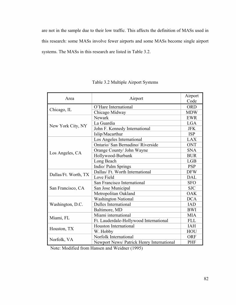
82
are not in the sample due to their low traffic. This affects the definition of MASs used in
this research: some MASs involve fewer airports and some MASs become single airport
systems. The MASs in this research are listed in Table 3.2.
Table 3.2 Multiple Airport Systems
Area Airport Airport Code
Chicago, IL O’Hare International ORD Chicago Midway MDW
New York City, NY
Newark EWR La Guardia LGA John F. Kennedy International JFK Islip/Macarthur ISP
Los Angeles, CA
Los Angeles International LAX Ontario/ San Bernadino/ Riverside ONT Orange County/ John Wayne SNA Hollywood-Burbank BUR Long Beach LGB Indio/ Palm Springs PSP
Dallas/Ft. Worth, TX Dallas/ Ft. Worth International DFW Love Field DAL
San Francisco, CA San Francisco International SFO San Jose Municipal SJC Metropolitan Oakland OAK
Washington, D.C. Washington National DCA Dulles International IAD Baltimore, MD BWI
Miami, FL Miami international MIA Ft. Lauderdale-Hollywood International FLL
Houston, TX Houston International IAH W. Hobby HOU
Norfolk, VA Norfolk International ORF Newport News/ Patrick Henry International PHF
Note: Modified from Hansen and Weidner (1995)
83
Summary Statistics
After the data were filtered, 1,660,569 route-quarter observations—including 96
thousand direct route-quarters and 1.56 million connecting route-quarters—remained to
estimate the model. The sample statistics are shown in Table 3.3.
The statistics for delay variables and the other variables are computed using data of
different time periods—1995 to 2003 for delays and 1996 to 2004 for other variables.
This is because lag delay variables are specified in the model. The lag delay variables for
year 1995 (i.e., delay variables of year 1994) are unavailable, and observations for 1995
thus are dropped. Delay variables of 2004 are not involved since they are not used in
estimation.
Market level variables, which are used to explain total demand of air routes, are
identical for all air routes of a market. The statistics for these variables, therefore, are
presented in terms of markets, instead of routes. The 1,660,569 route-quarter
observations corresponded to 213,917 market-quarters, 76,629 routes, and 6,133 markets.
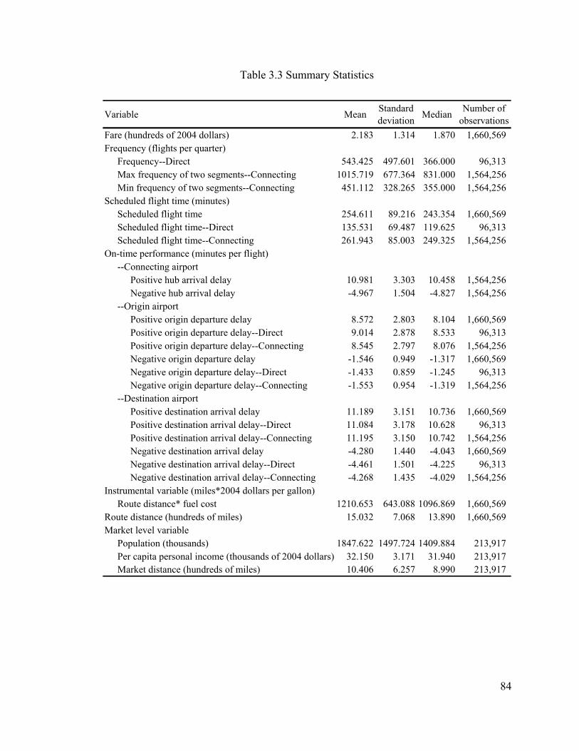
Table 3.3 Summary Statistics
Variable Mean Standard deviation Median Number of
observationsFare (hundreds of 2004 dollars) 2.183 1.314 1.870 1,660,569 Frequency (flights per quarter)
Frequency--Direct 543.425 497.601 366.000 96,313 Max frequency of two segments--Connecting 1015.719 677.364 831.000 1,564,256 Min frequency of two segments--Connecting 451.112 328.265 355.000 1,564,256
Scheduled flight time (minutes)Scheduled flight time 254.611 89.216 243.354 1,660,569 Scheduled flight time--Direct 135.531 69.487 119.625 96,313 Scheduled flight time--Connecting 261.943 85.003 249.325 1,564,256
On-time performance (minutes per flight)--Connecting airport
Positive hub arrival delay 10.981 3.303 10.458 1,564,256 Negative hub arrival delay -4.967 1.504 -4.827 1,564,256
--Origin airportPositive origin departure delay 8.572 2.803 8.104 1,660,569 Positive origin departure delay--Direct 9.014 2.878 8.533 96,313 Positive origin departure delay--Connecting 8.545 2.797 8.076 1,564,256 Negative origin departure delay -1.546 0.949 -1.317 1,660,569 Negative origin departure delay--Direct -1.433 0.859 -1.245 96,313 Negative origin departure delay--Connecting -1.553 0.954 -1.319 1,564,256
--Destination airportPositive destination arrival delay 11.189 3.151 10.736 1,660,569 Positive destination arrival delay--Direct 11.084 3.178 10.628 96,313 Positive destination arrival delay--Connecting 11.195 3.150 10.742 1,564,256 Negative destination arrival delay -4.280 1.440 -4.043 1,660,569 Negative destination arrival delay--Direct -4.461 1.501 -4.225 96,313 Negative destination arrival delay--Connecting -4.268 1.435 -4.029 1,564,256
Instrumental variable (miles*2004 dollars per gallon)Route distance* fuel cost 1210.653 643.088 1096.869 1,660,569
Route distance (hundreds of miles) 15.032 7.068 13.890 1,660,569 Market level variable
Population (thousands) 1847.622 1497.724 1409.884 213,917 Per capita personal income (thousands of 2004 dollars) 32.150 3.171 31.940 213,917 Market distance (hundreds of miles) 10.406 6.257 8.990 213,917
84

3.3 Model Estimation
The basic strategy for estimating aggregate logit models is to transform market
share functions and then estimate parameters by linear regression. For MNL models, the
market share of route r at time is given by Equation (2.3). The difference between
natural logarithms of market shares of two alternatives (
t
r and 'r ) is described as
Equation (3.7). Regressing the left hand side of the equation on differences of
explanatory variables gives estimates of the parameters of interest ( kβ ’s).
)()()ln()ln( ''1
' trrttkr
K
krtkktrrt xxMSMS ξξβ −+−=− ∑
=
(3.7)
Alternative-pairs need to be determined before running the regression. One simple
way is to use the outside good (non-air) alternative of which utility is normalized to zero
as the base alternative ( 'r ) for every route. As a result, Equation (3.7) can be simplified
to Equation (3.8), by which there is no need to differentiate explanatory variables.
Another way is to pick an alternative randomly as the base alternative ( 'r ) for other
alternatives.
rt
K
krtkktrt xMSMS ξβ +=− ∑
=10 )ln()ln( (3.8)
For NL models, estimations become more complicated. One possible solution is to
derive an equation, which is similar to Equation (3.8) but adding conditional market share
term(s) and its (their) coefficient(s), for each nesting structure. For example, the proposed
85
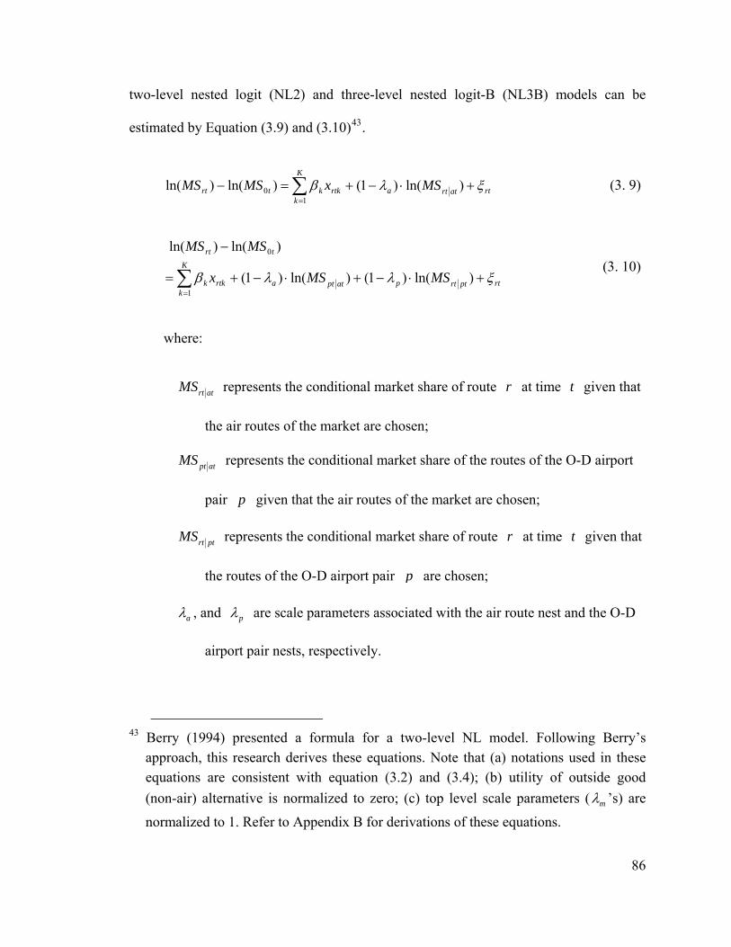
two-level nested logit (NL2) and three-level nested logit-B (NL3B) models can be
estimated by Equation (3.9) and (3.10)43.
rtatrta
K
krtkktrt MSxMSMS ξλβ +⋅−+=− ∑
=
)ln()1()ln()ln(1
0 (3. 9)
rtptrtpatpta
K
krtkk
trt
MSMSx
MSMS
ξλλβ +⋅−+⋅−+=
−
∑=
)ln()1()ln()1(
)ln()ln(
1
0
(3. 10)
where:
atrtMS represents the conditional market share of route r at time t given that
the air routes of the market are chosen;
atptMS represents the conditional market share of the routes of the O-D airport
pair p given that the air routes of the market are chosen;
ptrtMS represents the conditional market share of route r at time given that
the routes of the O-D airport pair
t
p are chosen;
aλ , and pλ are scale parameters associated with the air route nest and the O-D
airport pair nests, respectively.
43 Berry (1994) presented a formula for a two-level NL model. Following Berry’s
approach, this research derives these equations. Note that (a) notations used in these equations are consistent with equation (3.2) and (3.4); (b) utility of outside good (non-air) alternative is normalized to zero; (c) top level scale parameters ( mλ ’s) are
normalized to 1. Refer to Appendix B for derivations of these equations.
86
87
While equations like (3.9) and (3.10) seem to provide a convenient way to estimate
parameters, additional exogenous variables are required since the conditional market
shares are endogenous. This research does not choose this approach because finding valid
instrumental variables (IVs) becomes harder as the number of endogenous variables
requiring them increases. For instance, in order to estimate the NL3B model by Equation
(3.10), at least three (one for fare and two for conditional market shares) valid IVs are
needed. Recall that the proposed NL models include a four-level NL model, which needs
at least four valid IVs.
This research sequentially estimates NL models by decomposing NL models into
MNL models. More precisely, a nested logit model is estimated by nest and from bottom
level to top level. Within a nest, an MNL model is estimated by applying Equation (3.7)44,
in which the base alternative is randomly picked. Each level (except for the level
involving the fare variable, in which the method of two stage least squares is used), is
estimated by ordinary least squares (OLS) 45 and then the inclusive value(s) of nest(s) at
this level are calculated. Inclusive values of nests—which can be explained as the
expected maximum utility that potential travelers receive from those nests—of a lower
level are added into a higher level as an explanatory variable, of which the coefficient is
the ratio of scale parameters (a lower level scale parameter divided by a higher level scale
44 Since the models are estimated by applying Equation (3.7), all fixed effects with the
same values for all alternatives in a nest are differentiated out. Thus, the estimates implicitly take these effects into account. For example, market fixed effects are considered, although dummy variables for markets are not explicitly specified.
45 Standard errors of estimates that are robust to heteroskedasticity, serial correlation and market cluster effects are calculated for hypothesis tests.
88
parameter). Note that when estimating the NL models the utility of the non-air alternative
is normalized to zero, and the scale parameters of the bottom nests are set to one.
As discussed in chapter 2 and section 3.1.2, the air fare variable may be
endogenous, and thus the coefficients estimated by OLS method may be biased. This
research applies the instrumental variables method to solve the endogeneity problem. The
instrumental variable for air fare is defined as the product of the route distance and unit
jet fuel cost (in 2004 dollars per gallon). This variable captures the cost of offering the
service, and thus affects—at least to a certain extent—the price of the service. It is
expected to have no direct impact on market shares—the cost effect is accounted by air
fare. More specifically, since this research applies Equation (3.7) to estimate the models,
all variables used in estimation are differences between the variables of two alternatives.
Therefore, the cost variable difference of two routes is used as the IV for the fare
difference of the routes.
3.4 Estimation Results
Because lower-level nested logit and multinomial logit models are special cases of
higher-level nested logit models, this research estimates proposed nesting structures from
higher- level to lower-level nested logit models including multinomial logit models until
a model that is consistent with utility maximization is found. The NL4 and NL3A models
are not consistent with utility maximization. The NL3B model is found to be the
89
highest-level NL model that is consistent with utility maximization46. Thus, the results of
the NL3B model, including its experimental specifications and IV estimation, are
presented. One advantage of the sequential estimation is that estimation for higher-levels
is performed only after a preferred result for lower-level(s) is chosen. The detailed
estimation results, therefore, are discussed by level and then are combined in the
summary and discussions sub-section, in which the results of the MNL model with the
same explanatory variables are also presented for comparison purpose.
Level 3
As shown in Table 3.4, most coefficients of explanatory variables are statistically
significant and have expected signs, except for coefficients of origin departure delay of
connecting routes. Estimates from OLS method are listed in column (1) and (3).
Column (2) and (4) present results from IV estimation, in which air fare is instrumented.
Since the estimates from the same estimation method are close, results with significant
(in both OLS and IV estimations) variables—column (3) and (4)—are further discussed
and used to calculate inclusive values and estimate coefficients of higher levels.
46 The consistency is determined by the estimated ratio(s) of scale parameters of these
models, as discussed in section 3.1.1. Although the estimated ratios of scale parameters are different for different specifications, the conclusions of the consistency are the same under different experiments of specifications.
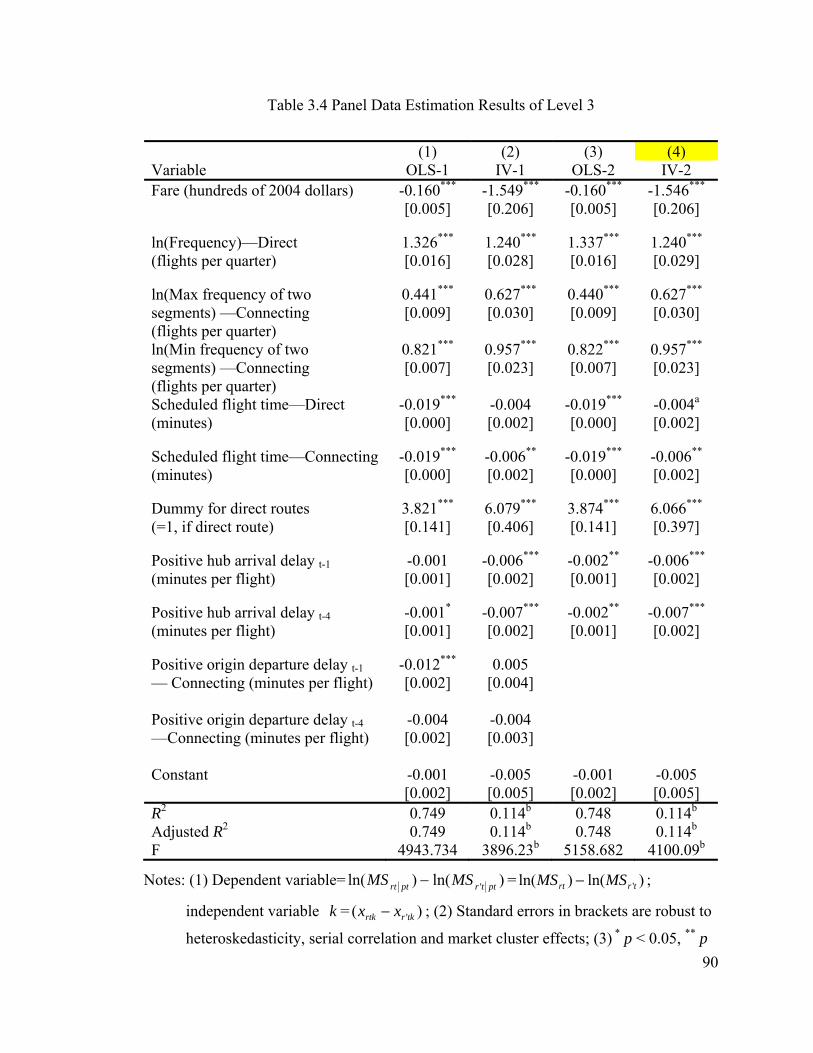
Table 3.4 Panel Data Estimation Results of Level 3
(1) (2) (3) (4) Variable OLS-1 IV-1 OLS-2 IV-2 Fare (hundreds of 2004 dollars) -0.160*** -1.549*** -0.160*** -1.546***
[0.005] [0.206] [0.005] [0.206]
ln(Frequency)—Direct (flights per quarter)
1.326*** 1.240*** 1.337*** 1.240*** [0.016] [0.028] [0.016] [0.029]
ln(Max frequency of two segments) —Connecting (flights per quarter)
0.441*** 0.627*** 0.440*** 0.627*** [0.009] [0.030] [0.009] [0.030]
ln(Min frequency of two segments) —Connecting (flights per quarter)
0.821*** 0.957*** 0.822*** 0.957*** [0.007] [0.023] [0.007] [0.023]
Scheduled flight time—Direct (minutes)
-0.019*** -0.004 -0.019*** -0.004a [0.000] [0.002] [0.000] [0.002]
Scheduled flight time—Connecting (minutes)
-0.019*** -0.006** -0.019*** -0.006** [0.000] [0.002] [0.000] [0.002]
Dummy for direct routes (=1, if direct route)
3.821*** 6.079*** 3.874*** 6.066*** [0.141] [0.406] [0.141] [0.397]
Positive hub arrival delay t-1 (minutes per flight)
-0.001 -0.006*** -0.002** -0.006*** [0.001] [0.002] [0.001] [0.002]
Positive hub arrival delay t-4 (minutes per flight)
-0.001* -0.007*** -0.002** -0.007*** [0.001] [0.002] [0.001] [0.002]
Positive origin departure delay t-1 — Connecting (minutes per flight)
-0.012*** 0.005 [0.002] [0.004]
Positive origin departure delay t-4 —Connecting (minutes per flight)
-0.004 -0.004 [0.002] [0.003]
Constant -0.001 -0.005 -0.001 -0.005 [0.002] [0.005] [0.002] [0.005] R2 0.749 0.114b 0.748 0.114b Adjusted R2 0.749 0.114b 0.748 0.114b F 4943.734 3896.23b 5158.682 4100.09b
Notes: (1) Dependent variable= )ln()ln( ' pttrptrt MSMS − = ;
independent variable = )
)ln()ln( 'trrt MSMS −
k ( 'tkrrtk xx − ; (2) Standard errors in brackets are robust to
heteroskedasticity, serial correlation and market cluster effects; (3) * p < 0.05, ** p 90
91
< 0.01, *** p < 0.001; (4) a: p-value=0.06; (5) b: Statistics of the first stage; (6) All regressions include 29 hub dummy variables, which are not shown here.
Although all estimated fare coefficients illustrate negative fare impacts on demand,
the fare coefficients from IV estimates are more reasonable. This can be seen from their
inferred values of travel time (VOTs). Recall that when air fare is endogenous47, its
coefficient estimated by OLS is more likely biased towards zero and thus the inferred
VOTs are overestimated. As shown in Table 3.5. Estimates from OLS method—column
(1), (3) and (5)—give unreasonable high VOTs, especially for values of scheduled flight
time: all the inferred values of scheduled flight time are greater than $614 per hour (39
times larger than the median wage rate of 2004). While literature on transportation
economics suggests a wide range of VOTs48, inferred VOTs from OLS estimates are still
out of these ranges. In contrast, fare coefficients from IV estimations are larger (in
absolute values) than those from OLS estimations, and provide sensible VOTs—at least
in the same order as those reported in the literature. For example, the value of scheduled
flight time of direct routes, given by the preferred model—column (4)—is $16.8 per hour
(105 percent of wage rate).
47 Tests for endogeneity of air fare based on the proposed instrumental variable appear
that air fare is endogenous for different specifications. 48 For example, Small and Winston (1999) summarized estimates of value of time by
transportation mode. The range, for different modes and trip types, is from 6 to 273 percent of wage rate. They also described that air travelers have a very high VOT—the VOT for air travelers for vacation trips is 149 percent of wage rate, estimated by Morrison and Winston (1985).
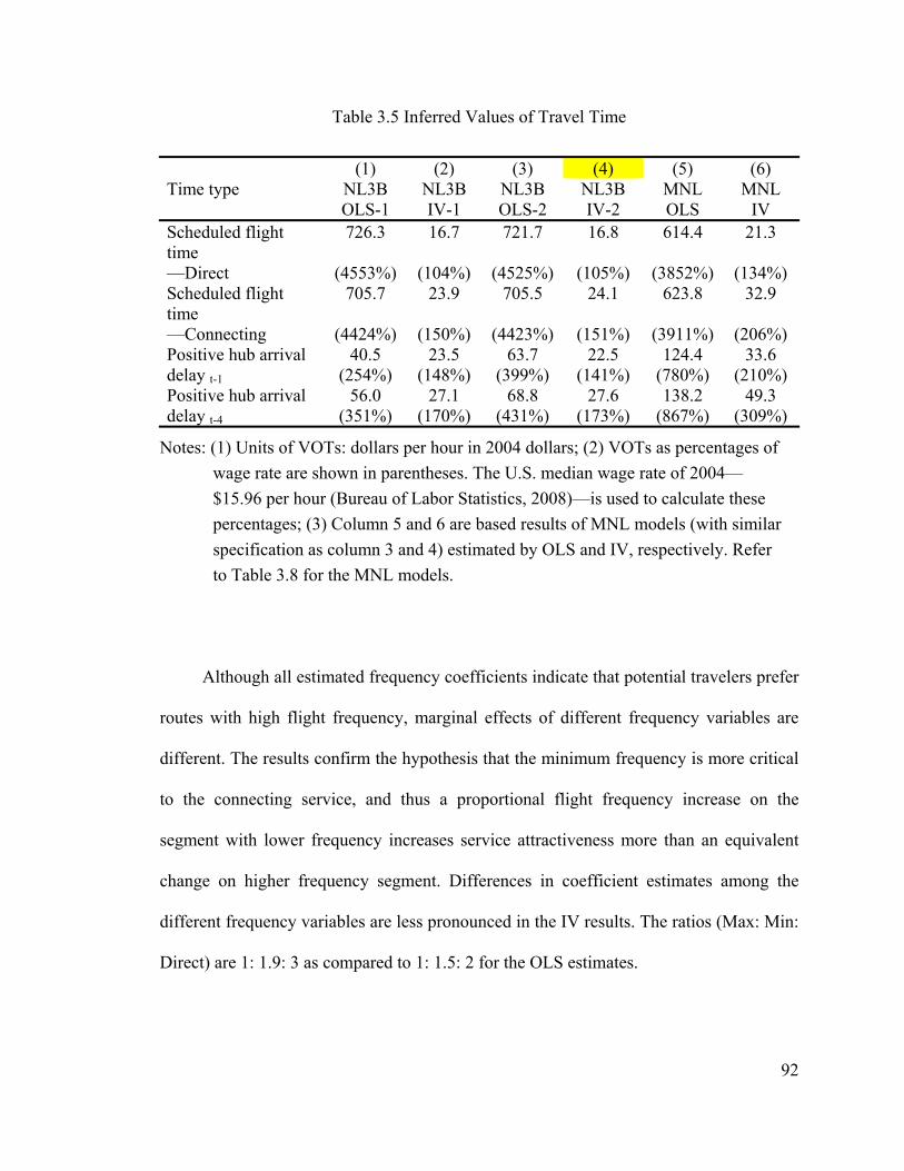
92
Table 3.5 Inferred Values of Travel Time
(1) (2) (3) (4) (5) (6) Time type NL3B
OLS-1 NL3B IV-1
NL3B OLS-2
NL3B IV-2
MNL OLS
MNL IV
Scheduled flight time —Direct
726.3 16.7 721.7 16.8 614.4 21.3
(4553%) (104%) (4525%) (105%) (3852%) (134%) Scheduled flight time —Connecting
705.7 23.9 705.5 24.1 623.8 32.9
(4424%) (150%) (4423%) (151%) (3911%) (206%) Positive hub arrival delay t-1
40.5 23.5 63.7 22.5 124.4 33.6 (254%) (148%) (399%) (141%) (780%) (210%)
Positive hub arrival delay t-4
56.0 27.1 68.8 27.6 138.2 49.3 (351%) (170%) (431%) (173%) (867%) (309%)
Notes: (1) Units of VOTs: dollars per hour in 2004 dollars; (2) VOTs as percentages of wage rate are shown in parentheses. The U.S. median wage rate of 2004— $15.96 per hour (Bureau of Labor Statistics, 2008)—is used to calculate these percentages; (3) Column 5 and 6 are based results of MNL models (with similar specification as column 3 and 4) estimated by OLS and IV, respectively. Refer to Table 3.8 for the MNL models.
Although all estimated frequency coefficients indicate that potential travelers prefer
routes with high flight frequency, marginal effects of different frequency variables are
different. The results confirm the hypothesis that the minimum frequency is more critical
to the connecting service, and thus a proportional flight frequency increase on the
segment with lower frequency increases service attractiveness more than an equivalent
change on higher frequency segment. Differences in coefficient estimates among the
different frequency variables are less pronounced in the IV results. The ratios (Max: Min:
Direct) are 1: 1.9: 3 as compared to 1: 1.5: 2 for the OLS estimates.
93
Although all coefficients of scheduled flight time indicate that travelers prefer
routes with shorter scheduled flight time, only the IV estimates suggest significantly
different marginal effects for different routing types. The IV estimates show that a
one-minute increase of scheduled flight time on connecting routes have a larger49 (about
1.4 times) impact of utility than that on direct routes, while the OLS estimates50 give
almost equal marginal effects for both routing types. As a result, the IV estimates imply
larger VOTs for connecting routes than for direct routes, given that the fare coefficients
are identical for both routing types. This result has two possible explanations. First,
travelers may feel more comfortable spending their time on direct flights than on
connecting ones. One the former, for example, they do not have to worry about missing
their subsequent flights due to flight delay and/or finding gates. Second, there may be
nonlinear effects of flight time that translate into the observed differences in coefficient
estimates. Given a city-pair market, scheduled flight time of a connecting route is
normally greater than that of a direct route. The nonlinear effects would make travelers
less likely to choose a connecting route with flight time much longer than that of a direct
route.
Positive hub arrival delay of one and four quarters before the decision quarter are
the only significant delay variables in our IV estimations, although many on-time
49 The hypothesis that the scheduled flight time coefficient of connecting routes is less
than or equal to that of direct routes is rejected at the 5% significance level. 50 Endogenous air fare may lead to inconsistent estimates, not only for the coefficients of
air fare but also for coefficients of other variables, when the OLS method is applied.
94
performance metrics51 were tried. This suggests that potential travelers make decisions
based on recent available information—including most recent impressions and seasonal
effects—on positive hub arrival delay. Compared to other delay metrics, positive hub
arrival delay receives more attention due to its higher penalty—missing connecting
flights. Another reason is that travelers usually have fewer chances of choosing origin
and destination airports than choosing hub airports. Note that the two hub delay variables
are specific for connecting routes—travelers choosing direct routes are free of hub delay.
When choosing among connecting routes, travelers avoid connecting at airports with high
expected delay in certain seasons.
For all specifications and estimation methods in Table 3.4, the coefficient
differences between the two hub delay variables are not statistically significant 52 ,
implying that potential travelers weigh on-time performance of the two periods (one and
four quarters before the decision quarter) equally. In addition, we expect that under
steady state, a one-minute hub delay increase has a larger impact on demand than an
equivalent change in scheduled flight time of a connecting route, because (1) delay
disturbs travelers’ original schedules and plans, and (2) travel time uncertainty may make
travelers uncomfortable. The NL3B-IV estimates confirm this hypothesis: the sum of two
51 As discussed in section 3.1.2, this research investigates (1) departure delays of origin
and hub airports, and arrival delays of hub and destination airports; (2) positive and negative delays; and (3) delays of one and four quarters before the decision quarter. The total number of delay variables is 16 (4*2*2).
52 All p-values are greater than 0.52.

95
hub delay coefficients is larger53 than the coefficient of scheduled flight time (both in
absolute values).
According to the data, arriving or departing earlier than schedule time does not
significantly make a route more attractive. The hypothesis that negative delay has smaller
marginal effects on demand than positive delay is confirmed, although this is mainly
because the coefficients of negative delays are zero.
After controlling for the other factors (such as fare, frequency, scheduled flight
time and delay) the coefficients of the direct route dummy variable still indicate that
potential travelers strongly prefer direct routes than connecting routes, regardless of
specifications and estimation methods.
Level 2
Estimation results for level 2 are shown in Table 3.6: column (1) to (4) are
estimates based on the inclusive values of level 3 estimated by IV; column (5), for
comparison purpose, specifies the same explanatory variables as column (4) except for
taking the inclusive values of level 3 estimated by OLS. The on-time performance effects
on O-D airport choice are examined at this level. As shown in column (1) to (3), none of
these delay variables are statistically significant. Thus, even when travelers are able to
choose O-D airports, on-time performance of these airports does not notably affect their
53 The null hypothesis that the sum of hub delay coefficients is less than or equal to the
coefficient of scheduled flight time (both in absolute values) is rejected at the 5% significance level (a one-tailed p-value of 0.032).
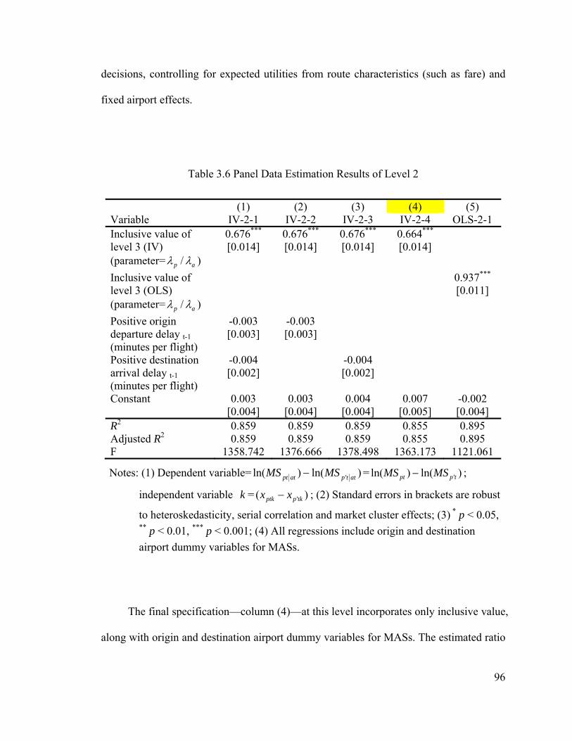
decisions, controlling for expected utilities from route characteristics (such as fare) and
fixed airport effects.
Table 3.6 Panel Data Estimation Results of Level 2
(1) (2) (3) (4) (5) Variable IV-2-1 IV-2-2 IV-2-3 IV-2-4 OLS-2-1 Inclusive value of level 3 (IV) (parameter= ap λλ / )
0.676*** 0.676*** 0.676*** 0.664*** [0.014] [0.014] [0.014] [0.014]
Inclusive value of level 3 (OLS) (parameter= ap λλ / )
0.937*** [0.011]
Positive origin departure delay t-1 (minutes per flight)
-0.003 -0.003 [0.003] [0.003]
Positive destination arrival delay t-1 (minutes per flight)
-0.004 -0.004 [0.002] [0.002]
Constant 0.003 0.003 0.004 0.007 -0.002
[0.004] [0.004] [0.004] [0.005] [0.004] R2 0.859 0.859 0.859 0.855 0.895 Adjusted R2 0.859 0.859 0.859 0.855 0.895 F 1358.742 1376.666 1378.498 1363.173 1121.061
Notes: (1) Dependent variable= )ln()ln( ' attpatpt MSMS − = ;
independent variable =
)ln()ln( 'tppt MSMS −
k )( 'tkpptk xx − ; (2) Standard errors in brackets are robust
to heteroskedasticity, serial correlation and market cluster effects; (3) * p < 0.05, ** p < 0.01, *** p < 0.001; (4) All regressions include origin and destination airport dummy variables for MASs.
The final specification—column (4)—at this level incorporates only inclusive value,
along with origin and destination airport dummy variables for MASs. The estimated ratio
96
of scale parameters ( ap λλ / ) based on the IV estimates of level 3 is 0.664, implying that
the correlation of the total utilities for two air routes sharing the same O-D airport pair is
moderate. However, the OLS estimates of level 3 lead to large (close to 1) ratio of scale
parameters ( ap λλ / ), implying that the correlation is very low. The large difference
between estimated ratios of scale parameters from two estimation methods and their
implications demonstrate the importance of correcting for the endogenous air fare
problem.
Level 1
Estimates of level 1 are presented in Table 3.7: column (1) and (3) list results based
on the OLS estimates of lower levels; column (2) and (4) show results associated with the
IV estimates of lower levels. Coefficients of income indicate that higher income level
generates more air trips, as expected. While column (1) and (2) assume fixed ratios of
scale parameters ( ma λλ / ), column (3) and (4) allow the ratios to change with market
distance —that is, the correlations of the total utilities for two O-D airport pairs may be
different for long-haul and short-haul markets.
97
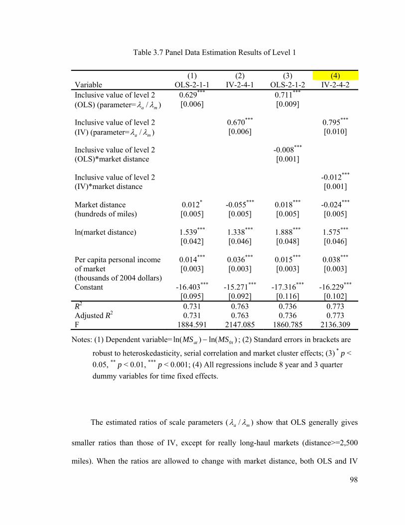
Table 3.7 Panel Data Estimation Results of Level 1
(1) (2) (3) (4) Variable OLS-2-1-1 IV-2-4-1 OLS-2-1-2 IV-2-4-2 Inclusive value of level 2 (OLS) (parameter= ma λλ / )
0.629*** 0.711*** [0.006] [0.009]
Inclusive value of level 2 (IV) (parameter= ma λλ / )
0.670*** 0.795*** [0.006] [0.010]
Inclusive value of level 2 (OLS)*market distance
-0.008*** [0.001]
Inclusive value of level 2 (IV)*market distance
-0.012*** [0.001]
Market distance (hundreds of miles)
0.012* -0.055*** 0.018*** -0.024*** [0.005] [0.005] [0.005] [0.005]
ln(market distance) 1.539*** 1.338*** 1.888*** 1.575***
[0.042] [0.046] [0.048] [0.046]
Per capita personal income of market (thousands of 2004 dollars)
0.014*** 0.036*** 0.015*** 0.038*** [0.003] [0.003] [0.003] [0.003]
Constant -16.403*** -15.271*** -17.316*** -16.229*** [0.095] [0.092] [0.116] [0.102] R2 0.731 0.763 0.736 0.773 Adjusted R2 0.731 0.763 0.736 0.773 F 1884.591 2147.085 1860.785 2136.309
Notes: (1) Dependent variable= )ln()ln( 0tat MSMS − ; (2) Standard errors in brackets are
robust to heteroskedasticity, serial correlation and market cluster effects; (3) * p < 0.05, ** p < 0.01, *** p < 0.001; (4) All regressions include 8 year and 3 quarter dummy variables for time fixed effects.
The estimated ratios of scale parameters ( ma λλ / ) show that OLS generally gives
smaller ratios than those of IV, except for really long-haul markets (distance>=2,500
miles). When the ratios are allowed to change with market distance, both OLS and IV
98
estimates of the ratios are consistent with utility-maximization (between 0 and 1) for a
reasonable range of market distance. For example, the ratio is 0.56, calculated from
column (4), for a city-pair with distance of 2000 miles. In addition, longer-haul markets
have lower ratios of scale parameters ( ma λλ / ), implying that the correlations of the total
utilities among O-D airport pairs (and thus among routes) in longer-haul markets are
higher. The higher correlation of two alternatives within a nest, the higher possibility that
the two alternatives substitute for each other—an alternative of other nest is less likely to
substitute for one of the two alternatives. Thus, the estimated ratios of both column (3)
and (4) indicate that in a longer-haul market route attribute changes are more likely to
shift traffic between air routes as opposed to affecting total air market traffic. In
shorter-haul markets, air routes, which have lower correlations, are more likely to
compete with other modes (non-air alternative, in different nest), such as auto and rail.
As discussed in section 3.1.2, the effect of market distance on air route demand
may be concave—the marginal effect may be decreasing as distance increases. Estimates
of column (1) and (2) show this concavity. Estimates of column (3) and (4) also yield
these effects, given a reasonable range of inclusive values of level 2. The distance effects
of column (3) and (4), which are partially determined by inclusive values, are visualized
in Figure 3.10. For each column, the inclusive values are either set to their mean values
or to the predicted values that are determined by a function of distance. Two regressions
of inclusive value on market distance are run to provide these two functions.
99
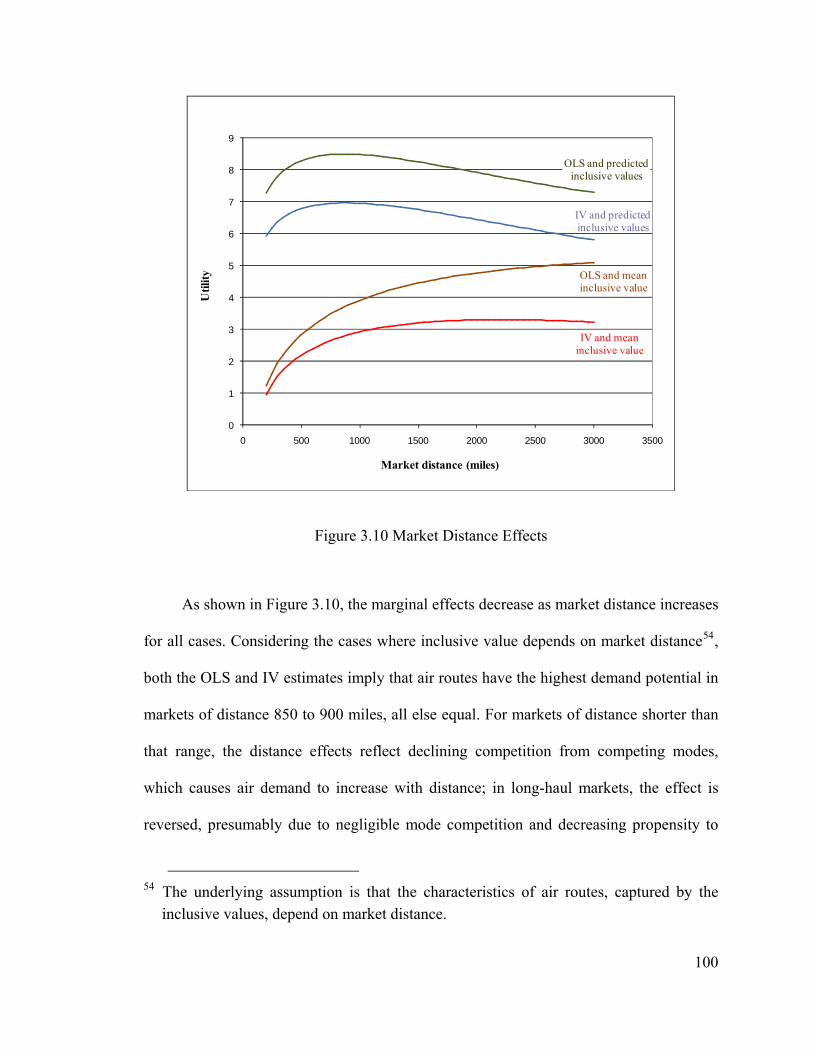
OLS and predicted inclusive values
IV and predicted inclusive values
0
1
2
3
4
5
6
7
8
9
0 500 1000 1500 2000 2500 3000 3500
Util
ity
Market distance (miles)
OLS and mean inclusive value
IV and mean inclusive value
Figure 3.10 Market Distance Effects
As shown in Figure 3.10, the marginal effects decrease as market distance increases
for all cases. Considering the cases where inclusive value depends on market distance54,
both the OLS and IV estimates imply that air routes have the highest demand potential in
markets of distance 850 to 900 miles, all else equal. For markets of distance shorter than
that range, the distance effects reflect declining competition from competing modes,
which causes air demand to increase with distance; in long-haul markets, the effect is
reversed, presumably due to negligible mode competition and decreasing propensity to
54 The underlying assumption is that the characteristics of air routes, captured by the
inclusive values, depend on market distance.
100
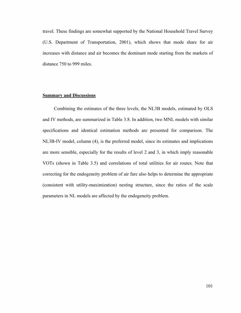
101
travel. These findings are somewhat supported by the National Household Travel Survey
(U.S. Department of Transportation, 2001), which shows that mode share for air
increases with distance and air becomes the dominant mode starting from the markets of
distance 750 to 999 miles.
Summary and Discussions
Combining the estimates of the three levels, the NL3B models, estimated by OLS
and IV methods, are summarized in Table 3.8. In addition, two MNL models with similar
specifications and identical estimation methods are presented for comparison. The
NL3B-IV model, column (4), is the preferred model, since its estimates and implications
are more sensible, especially for the results of level 2 and 3, in which imply reasonable
VOTs (shown in Table 3.5) and correlations of total utilities for air routes. Note that
correcting for the endogeneity problem of air fare also helps to determine the appropriate
(consistent with utility-maximization) nesting structure, since the ratios of the scale
parameters in NL models are affected by the endogeneity problem.
Table 3.8 Summary and Comparisons of Panel Data Estimation Results
(1) (2) (3) (4) Variable MNL
-OLS MNL -IV
NL3B -OLS
NL3B -IV
Fare (hundreds of 2004 dollars) -0.178*** -1.410*** -0.160*** -1.546*** [0.005] [0.411] [0.005] [0.206]
ln(Frequency)—Direct (flights per quarter)
1.282*** 1.212*** 1.337*** 1.240*** [0.015] [0.030] [0.016] [0.029]
ln(Max frequency of two segments)— Connecting (flights per quarter)
0.408*** 0.501*** 0.440*** 0.627*** [0.010] [0.034] [0.009] [0.030]
ln(Min frequency of two segments)— Connecting (flights per quarter)
0.793*** 0.883*** 0.822*** 0.957*** [0.007] [0.035] [0.007] [0.023]
Scheduled flight time—Direct (minutes)
-0.018*** -0.005 -0.019*** -0.004 [0.000] [0.004] [0.000] [0.002]
Scheduled flight time— Connecting (minutes)
-0.018*** -0.008* -0.019*** -0.006** [0.000] [0.004] [0.000] [0.002]
Dummy for direct routes (=1, if direct route)
3.353*** 4.477*** 3.874*** 6.066*** [0.145] [0.421] [0.141] [0.397]
Positive hub arrival delay t-1 (minutes per flight)
-0.004*** -0.008*** -0.002** -0.006*** [0.001] [0.002] [0.001] [0.002]
Positive hub arrival delay t-4 (minutes per flight)
-0.004*** -0.012*** -0.002** -0.007*** [0.001] [0.003] [0.001] [0.002]
Inclusive value of level 3 (parameter= ap λλ / )
0.937*** 0.664*** [0.011] [0.014]
Inclusive value of level 2 (parameter= ma λλ / )
0.711*** 0.795*** [0.009] [0.010]
Inclusive value of level 2 *market distance
-0.008*** -0.012*** [0.001] [0.001]
Market distance (hundreds of miles)
0.148*** 0.150*** 0.018*** -0.024*** [0.005] [0.010] [0.005] [0.005]
ln(market distance) 1.261*** 0.844*** 1.888*** 1.575*** [0.042] [0.145] [0.048] [0.046] Per capita personal income of market (thousands of 2004 dollars)
-0.665*** -0.637*** 0.015*** 0.038*** [0.006] [0.012] [0.003] [0.003]
Constant (level 1) 0.003 -0.001 -17.316*** -16.229*** [0.003] [0.006] [0.116] [0.102]
Notes: (1) Standard errors in brackets are robust to heteroskedasticity, serial correlation and market cluster effects; (2) * p < 0.05, ** p < 0.01, *** p < 0.001; (3) All regressions include hub dummy variables for connecting routes, origin and destination airport dummy variables for MASs, and year and quarter dummy variables for time fixed effects; (4) MNL models are estimated by Equation (3.7), in which the base alternative is randomly picked.
102
103
For the nesting structures, the NL3B models outperform the MNL models. First,
the NL3B models confirm the non-homogeneous correlations among alternatives,
implying that the MNL models incorrectly portray substitution patterns among routes.
Second, while the MNL models give similar patterns of coefficients for route level
variables, their income (a market level variable) coefficients are not reasonable—both
coefficients indicate that air routes become less attractive when income increases. One
possible explanation is that the income coefficients are estimated by comparing all air
routes with the non-air alternative in the NL3B models, but the income coefficients are
estimated by comparing individual routes with the non-air alternative in the MNL models.
When income increases, even though the total market share of air routes increases the
market share of a route may decrease, because the number of available routes may
increase with income. Similar situations may happen to other market level variables.
Therefore, the NL3B models are preferable.
Corrections for standard errors of higher level coefficients may be needed. Because
the sequential estimation does not carry variances of inclusive values into higher levels,
the standard errors of higher level coefficients in these levels are usually underestimated,
which may lead to invalid inferences and hypothesis tests. The standard errors presented
in Table 3.6, 3.7 and 3.8 are not corrected since most of the coefficients are very
significantly different from zero. However, all the standard errors reported in this
research are robust to heteroskedasticity, serial correlation and market cluster effects,
since error terms are unlikely to be independent and identically distributed.
104
Recall that to implement the proposed model this research assumes saturated
demand levels, depending on city-pair population. The results of lower levels are not
affected by the assumption because of the difference-in-differences estimation. Thus, the
impacts of the assumption are examined for level 1 only. All results of Table 3.7 are
based on the assumption that every unit of population may make 10 trips per quarter.
Taking column (4) of Table 3.7 as the base case and changing the assumption to different
numbers of trips lead to Table 3.9.
As shown in the Table 3.9, estimates change very little, except for the intercept.
Aside from these, the biggest differences are between column (1) and (2). The
assumption of column (1) is that every potential traveler may make 0.5 trips per quarter,
which is too close to the realized traffic level and not large enough to account for the
potential demand. Results of Tables 3.9 thus confirm that the setting of the saturated
demand only affects the estimated intercept of the market share model if the
proportionality factor is set large enough, as discussed in chapter 2.
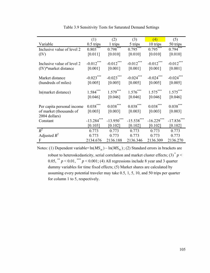
Table 3.9 Sensitivity Tests for Saturated Demand Settings
(1) (2) (3) (4) (5) Variable 0.5 trips 1 trips 5 trips 10 trips 50 trips Inclusive value of level 2 (IV)
0.803*** 0.798*** 0.795*** 0.795*** 0.794*** [0.011] [0.010] [0.010] [0.010] [0.010]
Inclusive value of level 2 (IV)*market distance
-0.012*** -0.012*** -0.012*** -0.012*** -0.012*** [0.001] [0.001] [0.001] [0.001] [0.001]
Market distance (hundreds of miles)
-0.023*** -0.023*** -0.024*** -0.024*** -0.024*** [0.005] [0.005] [0.005] [0.005] [0.005]
ln(market distance) 1.584*** 1.579*** 1.576*** 1.575*** 1.575***
[0.046] [0.046] [0.046] [0.046] [0.046]
Per capita personal income of market (thousands of 2004 dollars)
0.038*** 0.038*** 0.038*** 0.038*** 0.038*** [0.003] [0.003] [0.003] [0.003] [0.003]
Constant -13.284*** -13.950*** -15.538*** -16.229*** -17.836***
[0.103] [0.102] [0.102] [0.102] [0.102] R2 0.773 0.773 0.773 0.773 0.773 Adjusted R2 0.773 0.773 0.773 0.773 0.773 F 2134.676 2136.188 2136.346 2136.309 2136.270
Notes: (1) Dependent variable= )ln()ln( 0tat MSMS − ; (2) Standard errors in brackets are
robust to heteroskedasticity, serial correlation and market cluster effects; (3) * p < 0.05, ** p < 0.01, *** p < 0.001; (4) All regressions include 8 year and 3 quarter dummy variables for time fixed effects; (5) Market shares are calculated by assuming every potential traveler may take 0.5, 1, 5, 10, and 50 trips per quarter for column 1 to 5, respectively.
105
106
Chapter 4 Implications and Applications
Implications and applications of the estimated model are presented in this chapter.
Demand elasticities with respect to different variables, among which fare is particularly
of interest, are calculated and discussed first. Then, policy experiments on fare and
on-time performance are conducted to demonstrate applications of the model. Structural
changes over time are investigated in the last section.
4.1 Demand Elasticities
Elasticity is a useful tool in demand analysis. As a result, many estimates of air
travel demand elasticities, especially those with respect to fare, can be found in the
literature on transportation. Comparing demand elasticities from our models to previous
estimates helps us assess model validity. Elasticity, since it is dimensionless, also
provides a convenient way to compare the relative importance of causal factors. This is
particularly useful for nested logit models, in which direct comparisons between variables
of different nests is difficult, since the estimated coefficients are affected by scale
parameters.
The estimated parameters of models (Table 3.8) are used to calculate route and
market demand elasticities by simulation for each observation in the sample. These
elasticities are estimated numerically, instead of analytically, because for the proposed
107
model and variables, the numerical approach is simpler than the analytical approach55.
The elasticities weighted by the number of passengers are also calculated for comparisons.
In addition, the estimated elasticities with respect to fare and income are compared with
their counterparts in the literature.
The demand elasticity with respect to a variable is determined by calculating the
percentage change in demand resulting from one percent increase in the variable, holding
all other independent variables fixed. This method is used to find route demand
elasticities with respect to fare, frequency, and scheduled flight time. The market demand
elasticity with respect to a variable is calculated by increasing that variable by one
percent for all routes in a market and calculating the resulting percentage change in
market demand. For a route connecting at a specific hub, the route elasticity with respect
to positive hub arrival delay is calculated by changing the hub delay, which may affect
more than one route in an MAS.
4.1.1 Demand Elasticity with respect to Fare
Fare elasticities of market and route demand are summarized in Table 4.1. Since
potential travelers have more choices at route level than at market level, fare elasticities
of route demand are expected to be larger (in absolute values) than those of market
55 The formula for elasticity becomes much more complicated in higher level nesting
logit models. In addition, the variables of the model belong to several different aggregation levels (e.g. route, airport, and market levels), and variables of different levels need different formulas for their elasticities, if the analytical approach was chosen.
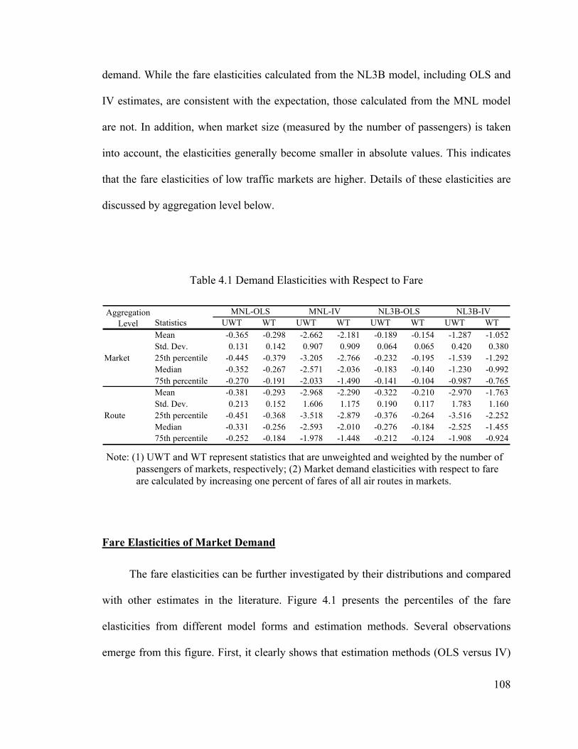
demand. While the fare elasticities calculated from the NL3B model, including OLS and
IV estimates, are consistent with the expectation, those calculated from the MNL model
are not. In addition, when market size (measured by the number of passengers) is taken
into account, the elasticities generally become smaller in absolute values. This indicates
that the fare elasticities of low traffic markets are higher. Details of these elasticities are
discussed by aggregation level below.
Table 4.1 Demand Elasticities with Respect to Fare
Statistics UWT WT UWT WT UWT WT UWT WTMean -0.365 -0.298 -2.662 -2.181 -0.189 -0.154 -1.287 -1.052Std. Dev. 0.131 0.142 0.907 0.909 0.064 0.065 0.420 0.380
Market 25th percentile -0.445 -0.379 -3.205 -2.766 -0.232 -0.195 -1.539 -1.292Median -0.352 -0.267 -2.571 -2.036 -0.183 -0.140 -1.230 -0.99275th percentile -0.270 -0.191 -2.033 -1.490 -0.141 -0.104 -0.987 -0.765Mean -0.381 -0.293 -2.968 -2.290 -0.322 -0.210 -2.970 -1.763Std. Dev. 0.213 0.152 1.606 1.175 0.190 0.117 1.783 1.160
Route 25th percentile -0.451 -0.368 -3.518 -2.879 -0.376 -0.264 -3.516 -2.252Median -0.331 -0.256 -2.593 -2.010 -0.276 -0.184 -2.525 -1.45575th percentile -0.252 -0.184 -1.978 -1.448 -0.212 -0.124 -1.908 -0.924
MNL-OLS MNL-IV NL3B-OLS NL3B-IVAggregation Level
Note: (1) UWT and WT represent statistics that are unweighted and weighted by the number of
passengers of markets, respectively; (2) Market demand elasticities with respect to fare are calculated by increasing one percent of fares of all air routes in markets.
Fare Elasticities of Market Demand
The fare elasticities can be further investigated by their distributions and compared
with other estimates in the literature. Figure 4.1 presents the percentiles of the fare
elasticities from different model forms and estimation methods. Several observations
emerge from this figure. First, it clearly shows that estimation methods (OLS versus IV)
108
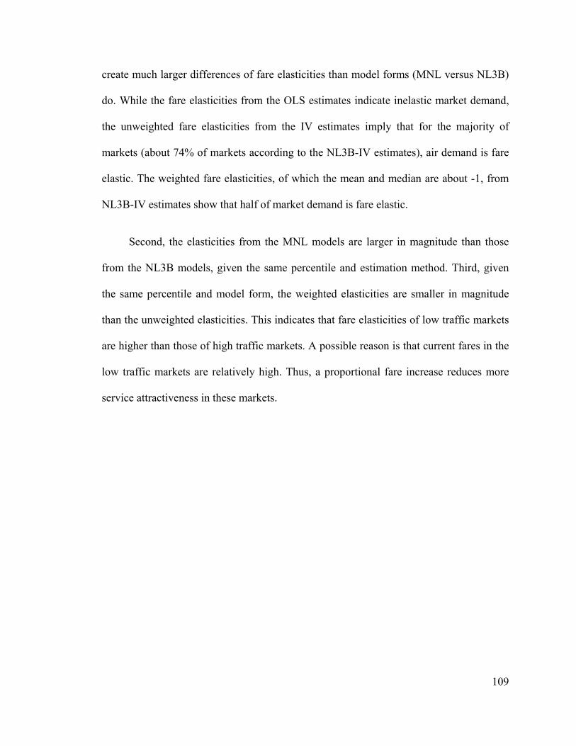
109
create much larger differences of fare elasticities than model forms (MNL versus NL3B)
do. While the fare elasticities from the OLS estimates indicate inelastic market demand,
the unweighted fare elasticities from the IV estimates imply that for the majority of
markets (about 74% of markets according to the NL3B-IV estimates), air demand is fare
elastic. The weighted fare elasticities, of which the mean and median are about -1, from
NL3B-IV estimates show that half of market demand is fare elastic.
Second, the elasticities from the MNL models are larger in magnitude than those
from the NL3B models, given the same percentile and estimation method. Third, given
the same percentile and model form, the weighted elasticities are smaller in magnitude
than the unweighted elasticities. This indicates that fare elasticities of low traffic markets
are higher than those of high traffic markets. A possible reason is that current fares in the
low traffic markets are relatively high. Thus, a proportional fare increase reduces more
service attractiveness in these markets.
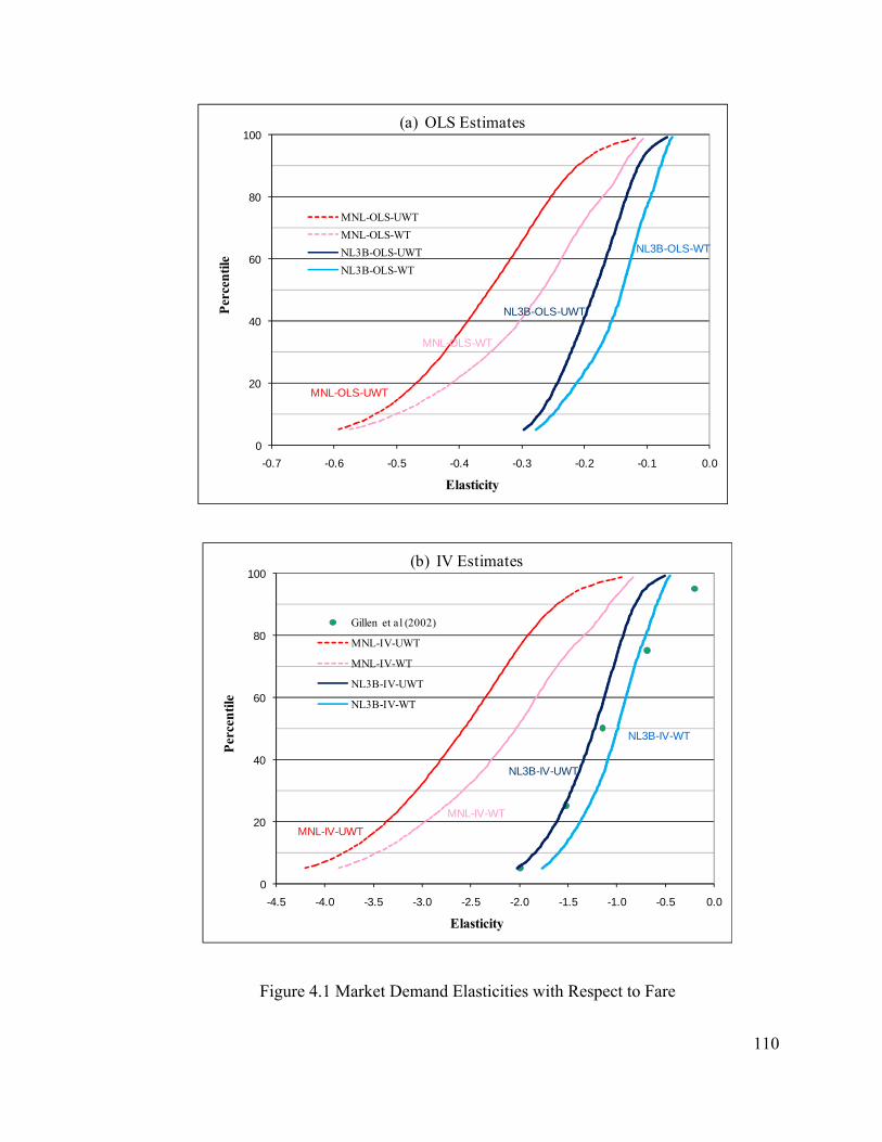
110
MNL-OLS-UWT
MNL-OLS-WT
NL3B-OLS-UWT
NL3B-OLS-WT
0
20
40
60
80
100
-0.7 -0.6 -0.5 -0.4 -0.3 -0.2 -0.1 0.0
Perc
entil
e
Elasticity
(a) OLS Estimates
MNL-OLS-UWTMNL-OLS-WTNL3B-OLS-UWTNL3B-OLS-WT
MNL-IV-UWTMNL-IV-WT
NL3B-IV-UWT
NL3B-IV-WT
0
20
40
60
80
100
-4.5 -4.0 -3.5 -3.0 -2.5 -2.0 -1.5 -1.0 -0.5 0.0
Perc
entil
e
Elasticity
(b) IV Estimates
Gillen et al (2002)
MNL-IV-UWT
MNL-IV-WT
NL3B-IV-UWT
NL3B-IV-WT
Figure 4.1 Market Demand Elasticities with Respect to Fare

111
The fare elasticities from the NL3B-IV estimates are supported by the above
observations and also by findings in the literature. Oum et al (1986) reported that fare
elasticities of market demand56 were -1.51 and -1.15 for vacation and non-vacation
markets, respectively. These estimates are within the range of the elasticities from the
NL3B-IV estimates. In addition, the fare elasticity percentiles taken from Gillen et al
(2002)57 are plotted in panel (b) of Figure 4.1, which demonstrates that the NL3B-IV
estimates provide fare elasticities closer to those from other studies, especially for larger
absolute elasticities (smaller percentiles).
It is interesting to observe that the elasticities from the NL3B-IV estimates accord
with the variation of elasticities from other studies. One of the reasons may be that
varieties of markets are involved in our sample—covering most domestic markets of the
United States for 10 years. The elasticity distribution from Gillen et al (2002) consists of
elasticities from different studies, which also involve different study regions, market
distance, and time periods.
Fare Elasticities of Route Demand
As shown in Table 4.1, the unweighted means of fare elasticities from both IV
estimates are about -2.9. Although the weighted means become smaller in absolute values,
all the means of the fare elasticities from the IV estimates indicate that route demand is
fare elastic. All the means of fare elasticities from the OLS estimates, however, suggest
56 They used the term “aggregate route demand” for the market demand. 57 They summarized 274 estimates, taken from 22 studies, of fare elasticities of market
demand.
that route demand is fare inelastic. The fare elasticities from the IV estimates are better
supported by the inferred values-of-time (Table 3.5) and the literature (discussed below).
The distributions of fare elasticities of route demand from the IV estimates plotted
in Figure 4.2, in which patterns similar to Figure 4.1 can be observed. In addition, these
percentiles imply that the distributions of fare elasticities of route demand are not
symmetric and have longer left tails58. This is sensible since fare elasticities are more
likely to be bounded on the right sides (e.g. less than zero).
MNL-IV-UWT
MNL-IV-WT
NL3B-IV-UWT
NL3B-IV-WT
0
20
40
60
80
100
-7 -6 -5 -4 -3 -2 -1 0
Perc
entil
e
Elasticity
MNL-IV-UWT
MNL-IV-WT
NL3B-IV-UWT
NL3B-IV-WT
Figure 4.2 Route Demand Elasticities with Respect to Fare (IV Estimates)
58 This is consistent with the findings in the literature, such as Gillen et al (2002).
112
113
Direct comparisons of estimates from literature and this research cannot be made
because most fare elasticities available in the literature are estimates for air market
demand or for airline demand. However, some guidelines for ranges of fare elasticities
are available.
One would expect that elasticities of route demand should be larger (in absolute
values) than those of market demand, since people generally have higher flexibility in air
routes as long as they can arrive their destinations, and changing to other modes or trip
cancelations are less likely to be their choices. Summarizing from the literature on air
market demand, Gillen et al (2002) reported that the medians of the fare elasticities for
different trip lengths and trip purposes range from -0.70 to -1.52. The fare elasticities of
route demand from the OLS estimates are, like those of market demand, too low—most
of them are smaller (in absolute values) than those of market demand from Gillen et al
(2002). The fare elasticities from the IV estimates seem more reasonable: (1) the medians
are -2.95 (from MNL-IV) and -2.53 (from NL3B); (2) most of them are less than -1
indicating that potential travelers are fare elastic.
Fare elasticities of route demand are comparable to some degree to elasticities of
airline demand (in a particular market) reported in the literature. First, for monopolistic
routes, route demands are equivalent to airline demands. For example, airlines serving the
same market generally offer competing routes each connecting at their respective hubs,
so that each route corresponds to one airline. When airlines compete with each other on
the same routes, elasticities of airline demand should be higher than those of route
114
demand. This may be offset, however, by airline brand loyalty (e.g. due to frequent flyer
programs), which reduces airline demand elasticities.
The fare elasticities of route demand from the IV estimates (Figure 4.2) are
consistent with these expectations. For most routes, the estimated absolute fare
elasticities are larger than those of market demand, and close to smaller than those of
airline demand, compared with the estimates of Oum et al (1993). Oum et al (1993)
estimated fare elasticities of market demand 59 and computed airline specific fare
elasticities using the estimated conduct parameters. The medians of their fare elasticities
are -1.54 for market demand and -2.99 for airline demand. Our corresponding values are
-1.23 and -2.53.
4.1.2 Demand Elasticity with respect to other Variables
In this section, income and distance elasticities of market demand, and route
demand elasticities with respect to frequency, and scheduled flight time, hub delay are
discussed. The income and distance elasticities are presented in Table 4.2. The weighted
fare and distance elasticities become smaller in absolute values, compared to the
unweighted elasticities. This indicates that the distance elasticities of low traffic markets
are higher. However, the weighted income elasticities are larger, suggesting that the
income elasticities of low traffic markets are lower.
59 They used the term “aggregate route demand” for the market demand.
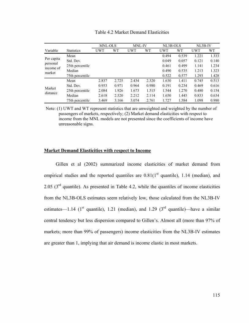
Table 4.2 Market Demand Elasticities
Variable Statistics UWT WT UWT WT UWT WT UWT WTMean 0.494 0.539 1.221 1.333Std. Dev. 0.049 0.057 0.121 0.14025th percentile 0.461 0.499 1.141 1.234Median 0.490 0.535 1.213 1.32375th percentile 0.522 0.577 1.293 1.428Mean 2.837 2.725 2.434 2.320 1.630 1.411 0.745 0.513Std. Dev. 0.953 0.971 0.964 0.980 0.191 0.234 0.469 0.61625th percentile 2.084 1.926 1.673 1.515 1.544 1.270 0.480 0.154Median 2.618 2.520 2.212 2.114 1.650 1.445 0.833 0.63475th percentile 3.469 3.166 3.074 2.761 1.727 1.584 1.098 0.980
Per capita personal income of market
Market distance
MNL-OLS MNL-IV NL3B-OLS NL3B-IV
Note: (1) UWT and WT represent statistics that are unweighted and weighted by the number of
passengers of markets, respectively; (2) Market demand elasticities with respect to income from the MNL models are not presented since the coefficients of income have unreasonable signs.
Market Demand Elasticities with respect to Income
Gillen et al (2002) summarized income elasticities of market demand from
empirical studies and the reported quantiles are 0.81(1st quantile), 1.14 (median), and
2.05 (3rd quantile). As presented in Table 4.2, while the quantiles of income elasticities
from the NL3B-OLS estimates seem relatively low, those calculated from the NL3B-IV
estimates—1.14 (1st quantile), 1.21 (median), and 1.29 (3rd quantile)—have a similar
central tendency but less dispersion compared to Gillen’s. Almost all (more than 97% of
markets; more than 99% of passengers) income elasticities from the NL3B-IV estimates
are greater than 1, implying that air demand is income elastic in most markets.
115
116
Market Demand Elasticities with respect to Market Distance
As shown in Table 4.2, the NL3B model and the IV estimation generally yield the
smallest distance elasticities of market demand. As a result, the elasticities computed
from the NL3B-IV estimates are smaller than those from the other estimates. While the
majority of the distance elasticities from the NL3B-IV estimates are positive, about 8% of
markets (18% in terms of passenger traffic) have negative demand elasticities with
respect to market distance. This can be explained by the concave relationship between
market distance and air demand, as found in Table 3.8.
Distance effects from the NL3B-IV estimates for markets with similar distance may
vary, since they also depend on inclusive values, which represent service levels of air
routes. Demand elasticities with respect to market distance can help to understand the
distance effects of individual markets. Figure 4.3 summarizes the incidence of negative
distance elasticities by distance category. Three main generalizations emerge from the
figure. First, over 99.5% of markets with distance less than 1200 miles have positive
distance elasticities. That is, for two markets with distance less than 1200 miles, the
longer distance market is expected to have higher air demand, all else (such as
population, income, and service levels) being equal.
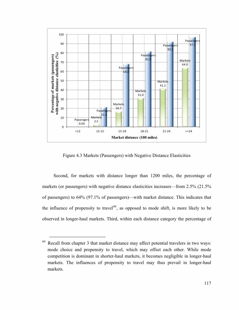
Markets2.5
Markets16.7
Markets31.0
Markets41.2
Markets64.0
Passengers0.04
Passengers21.5
Passengers68.0
Passengers81.5
Passengers92.2
Passengers97.1
0
10
20
30
40
50
60
70
80
90
100
<12 12‐15 15‐18 18‐21 21‐24 >=24
Perc
enta
ge o
f mar
kets
(pas
seng
ers)
w
ith n
egat
ive
dist
ance
ela
stic
ities
(%
)
Market distance (100 miles)
Figure 4.3 Markets (Passengers) with Negative Distance Elasticities
Second, for markets with distance longer than 1200 miles, the percentage of
markets (or passengers) with negative distance elasticities increases—from 2.5% (21.5%
of passengers) to 64% (97.1% of passengers)—with market distance. This indicates that
the influence of propensity to travel60, as opposed to mode shift, is more likely to be
observed in longer-haul markets. Third, within each distance category the percentage of
60 Recall from chapter 3 that market distance may affect potential travelers in two ways:
mode choice and propensity to travel, which may offset each other. While mode competition is dominant in shorter-haul markets, it becomes negligible in longer-haul markets. The influences of propensity to travel may thus prevail in longer-haul markets.
117
118
passengers with negative distance elasticities is higher than the percentage of markets
with negative distance elasticities. This implies that negative distance elasticities are
more likely to be found in higher traffic markets, which are usually better served and thus
have larger inclusive values61. All else being equal, while the influence of declining
propensity to travel is more pronounced in better served markets, the influence of mode
competition is stronger in minor markets.
Route Demand Elasticities with respect to other Variables
The route demand elasticities with respect to other variables are shown in Table 4.3.
Elasticities from the preferred model (NL3B-IV) indicate that fare (shown in Table 4.1)
and hub delay have the highest and lowest, respectively, impacts on route demand.
As suggested by Table 4.3, route demand elasticities with respect to frequency
variables are stable across routes—mainly due to their logarithmic functional form. The
estimated frequency elasticities, however, vary slightly depending on model forms and
estimation methods. The NL3 model and the IV estimation generally yield smaller
frequency elasticities for direct routes but larger frequency elasticities for connecting
routes. As a result, the elasticity differences of three frequency variables from the
NL3B-IV model are smaller than those from other models. In addition, the frequency
elasticities from the NL3B-IV model indicate that for most routes adding one percent of
61 As shown in Table 3.8, the coefficient (from NL3B-IV estimates) of the interaction
term of distance and inclusive value is negative, which may lead to negative distance elasticities when the inclusive value is large.
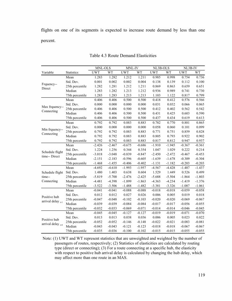
flights on one of its segments is expected to increase route demand by less than one
percent.
Table 4.3 Route Demand Elasticities
Variable Statistics UWT WT UWT WT UWT WT UWT WTMean 1.283 1.282 1.212 1.211 0.985 0.998 0.754 0.736Std. Dev. 0.001 0.002 0.002 0.004 0.138 0.139 0.112 0.10025th percentile 1.282 1.281 1.212 1.211 0.869 0.863 0.659 0.651Median 1.283 1.282 1.213 1.212 0.936 0.989 0.741 0.73075th percentile 1.283 1.283 1.213 1.213 1.103 1.122 0.817 0.799Mean 0.406 0.406 0.500 0.500 0.418 0.412 0.576 0.566Std. Dev. 0.000 0.000 0.000 0.000 0.031 0.032 0.066 0.06525th percentile 0.406 0.406 0.500 0.500 0.412 0.402 0.562 0.542Median 0.406 0.406 0.500 0.500 0.431 0.425 0.603 0.59075th percentile 0.406 0.406 0.500 0.500 0.437 0.434 0.619 0.613Mean 0.792 0.792 0.883 0.883 0.782 0.770 0.881 0.865Std. Dev. 0.000 0.000 0.000 0.000 0.058 0.060 0.101 0.09925th percentile 0.792 0.792 0.883 0.883 0.771 0.751 0.859 0.828Median 0.792 0.792 0.883 0.883 0.805 0.793 0.922 0.90275th percentile 0.792 0.792 0.883 0.883 0.817 0.812 0.947 0.937Mean -2.426 -2.467 -0.675 -0.686 -1.910 -1.945 -0.367 -0.361Std. Dev. 1.224 1.256 0.344 0.354 1.047 1.029 0.222 0.21425th percentile -3.018 -3.048 -0.839 -0.847 -2.450 -2.472 -0.467 -0.453Median -2.151 -2.183 -0.596 -0.605 -1.639 -1.678 -0.309 -0.30475th percentile -1.468 -1.455 -0.406 -0.402 -1.131 -1.182 -0.203 -0.203Mean -4.692 -4.610 -1.993 -1.957 -4.567 -4.428 -1.487 -1.437Std. Dev. 1.480 1.403 0.638 0.604 1.529 1.449 0.526 0.49925th percentile -5.819 -5.700 -2.476 -2.425 -5.688 -5.504 -1.864 -1.803Median -4.481 -4.398 -1.899 -1.863 -4.363 -4.234 -1.419 -1.37675th percentile -3.522 -3.506 -1.488 -1.482 -3.381 -3.326 -1.087 -1.061Mean -0.041 -0.041 -0.088 -0.088 -0.018 -0.018 -0.059 -0.058Std. Dev. 0.012 0.012 0.027 0.026 0.006 0.005 0.019 0.01825th percentile -0.047 -0.048 -0.102 -0.103 -0.020 -0.020 -0.069 -0.067Median -0.039 -0.039 -0.084 -0.084 -0.017 -0.017 -0.056 -0.05575th percentile -0.032 -0.033 -0.069 -0.071 -0.014 -0.014 -0.046 -0.045Mean -0.045 -0.045 -0.127 -0.127 -0.019 -0.019 -0.071 -0.070Std. Dev. 0.013 0.013 0.038 0.036 0.006 0.005 0.023 0.02225th percentile -0.052 -0.052 -0.146 -0.148 -0.022 -0.021 -0.083 -0.081Median -0.043 -0.043 -0.121 -0.123 -0.018 -0.018 -0.067 -0.06775th percentile -0.035 -0.036 -0.100 -0.102 -0.015 -0.015 -0.055 -0.055
Positive hub arrival delay t-4
Positive hub arrival delay t-1
Schedule flight time--Connecting
Schedule flight time-- Direct
Min frquency--Connecting
Frquency-- Direct
Max frquency--Connecting
MNL-OLS MNL-IV NL3B-OLS NL3B-IV
Note: (1) UWT and WT represent statistics that are unweighted and weighted by the number of
passengers of routes, respectively; (2) Statistics of elasticities are calculated by routing type (direct or connecting); (3) For a route connecting at a specific hub, the elasticity with respect to positive hub arrival delay is calculated by changing the hub delay, which may affect more than one route in an MAS.
119
120
The NL3B model and the IV estimation lead to smaller (in absolute values)
scheduled flight time elasticities for both direct and connecting routes. The elasticities
from the NL3B-IV model suggest that shortening one percent of scheduled flight time is
expected to increase route demand by more than one percent for connecting routes, but
less than one percent for direct routes.
Hub delay elasticities from different model forms and estimation methods are much
smaller in absolute values than elasticities with respect to other variables. For example,
the median elasticity with respect to hub delay of previous quarter is only -0.05662,
according to the elasticities from the NL3B-IV estimates. This implies that potential
travelers are not very sensitive to hub delay. Therefore, potential travelers will not
significantly benefit from delay improvements, unless the delay reductions are large.
4.2 Policy Experiments
We conducted policy experiments on fare and on-time performance to demonstrate
applications of the model. We based these on 2004 data63. As the IV estimates lead to
62 If we consider hub delay elasticities under stead state, the number is approximately
doubled, since elasticities with respect to the two hub delay variables are close to each other. The small elasticities are not surprising since a one-percent increase in delay only increase travel time by a few seconds.
63 The number of passengers in the data set is a 10 percent sample from U.S. DOT’s Airline Origin and Destination Survey (DB1B). All the traffic levels presented in the experiments are converted into 100 percent levels by multiplying a factor of 10.
121
more reasonable values-of-time and own-elasticities of demand than OLS estimates do,
two forms of models estimated by IV method (MNL-IV and NL3B-IV) are compared in
the policy experiments in order to show their differences in substitution patterns of
alternatives.
4.2.1 Fare Experiment
This experiment illustrates how the model can be used to capture impacts of fare
changes that might arise from a change in tax policy. For each scenario, a fixed per
segment fare increase is set. Therefore, the total fare change of a route is equal to the
increase for a direct route, or twice the increase for a connecting route. Assuming all air
routes are affected by the fare changes, changes in air passenger traffic volumes—
including traffic volumes on direct and connecting routes—are used to assess the
impacts.
In practice, these scenarios could happen when a segment-related factor that affects
fares changes. The factor could be a fixed charge for passengers based on flight segment
(or enplanement). Domestic flight segment tax and passenger facility charge (PFC) are
examples. When the segment tax or PFC is raised (or reduced), airlines may pass the
change (or a proportion of the change) to passengers. Thus, the total payments of
passengers are changed. In this experiment, fare changes—including increase of 2 and 4
dollars per segment are used in scenarios. Using the model to analyze the impacts of
different charge schemes is a possible extension of this experiment. For instance, a
“revenue neutral” mix of segment fee increases and percentage ticket tax reductions
could be tested.
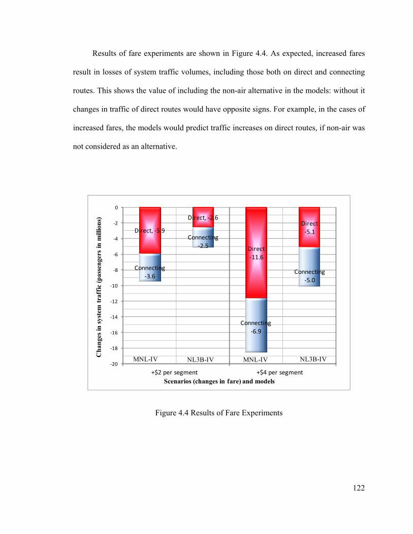
Results of fare experiments are shown in Figure 4.4. As expected, increased fares
result in losses of system traffic volumes, including those both on direct and connecting
routes. This shows the value of including the non-air alternative in the models: without it
changes in traffic of direct routes would have opposite signs. For example, in the cases of
increased fares, the models would predict traffic increases on direct routes, if non-air was
not considered as an alternative.
Direct, ‐5.9
Direct, ‐2.6
Direct‐11.6
Direct‐5.1
Connecting‐3.6
Connecting‐2.5
Connecting‐6.9
Connecting‐5.0
‐20
‐18
‐16
‐14
‐12
‐10
‐8
‐6
‐4
‐2
0
+$2 per segment +$4 per segment
Cha
nges
in sy
stem
traf
fic (p
asse
nger
s in
mill
ions
)
Scenarios (changes in fare) and models
MNL-IV NL3B-IVNL3B-IVMNL-IV
Figure 4.4 Results of Fare Experiments
122
123
Comparing results of different scenarios within the same model form, the changes
in traffic increase slightly less than proportionally, as fare changes increase. For instance,
according to NL3B estimates, the air systems are expected to lose 5.1 and 10.1 million
passengers if fares increase $2 and $4 per segment, respectively.
The predicted total traffic changes from the MNL-IV model are larger than those
from the NL3B model. This can also be seen from the market demand elasticities with
respect to fare (Table 4.1 and Figure 4.1). Second, while the MNL-IV model predicts
larger (about 1.6 times) traffic changes on direct routes than on connecting routes, the
NL3B-IV model yields almost equal traffic changes on both routing types. Recall that the
estimated scale parameters (in Table 3.8) have confirmed that potential passengers are
more likely to switch from connecting routes to direct route than to non-air alternative.
Although direct routes lose their original traffic volumes to the non-air alternative, they
gain traffic volumes from connecting routes instead, because fare changes of connecting
routes are larger. Thus, the MNL-IV model very likely overestimates64 (in absolute value)
the traffic changes on direct routes due to the IIA assumption.
64 This argument can be more directly supported by delay experiments (in section 4.2.2),
in which utilities of direct routes are not affected by hub delays at all.
124
4.2.2 Delay Experiments
A tremendous amount of money has been and will be spent on improvements of air
transportation systems. Delay reduction is one of the improvement measures. Applying
the proposed model, benefits of delay reductions, which are important for justifying the
investments, can be quantified. In this section, two delay experiments are performed to
demonstrate how the model can be used to evaluate impacts of delay changes.
The first one considers the case of system delay changes of all 30 hub
airports—all connecting routes are influenced by the changes. A practical example of this
case is system improvements, such as the Next Generation Air Transportation System
(NextGen) program, on all benchmark airports. The second delay experiment focuses on
delay changes at a specific hub airport—using Chicago O’Hare International Airport
(ORD) as an example. The planned airport capacity enhancement at ORD may result in
this. The model can also be used to evaluate the system-wide effects of the project, not
only the impacts on ORD.
According to the specifications and the estimated results, quarterly demand levels
of year 2004 depend on quarterly hub delays of year 2003 and 2004. Thus, for each
scenario, a percentage change of 2003 and 2004 hub delay is set. Four scenarios are
examined in each experiment: 25 and 50 percent increases and decreases in original hub
delay. Changes in air passenger traffic volumes and their components are also used to
assess the impacts.
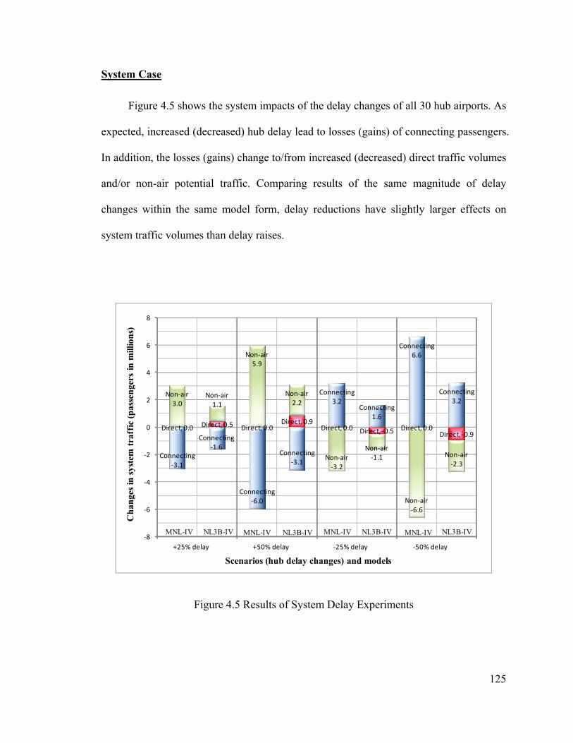
System Case
Figure 4.5 shows the system impacts of the delay changes of all 30 hub airports. As
expected, increased (decreased) hub delay lead to losses (gains) of connecting passengers.
In addition, the losses (gains) change to/from increased (decreased) direct traffic volumes
and/or non-air potential traffic. Comparing results of the same magnitude of delay
changes within the same model form, delay reductions have slightly larger effects on
system traffic volumes than delay raises.
Direct, 0.0 Direct, 0.5 Direct, 0.0Direct, 0.9
Direct, 0.0 Direct, ‐0.5 Direct, 0.0Direct, ‐0.9
Non‐air3.0
Non‐air1.1
Non‐air5.9
Non‐air2.2
Non‐air‐3.2
Non‐air‐1.1
Non‐air‐6.6
Non‐air‐2.3
Connecting‐3.1
Connecting‐1.6
Connecting‐6.0
Connecting‐3.1
Connecting3.2
Connecting1.6
Connecting6.6
Connecting3.2
‐8
‐6
‐4
‐2
0
2
4
6
8
+25% delay +50% delay ‐25% delay ‐50% delay
Cha
nges
in sy
stem
traf
fic (p
asse
nger
s in
mill
ions
)
Scenarios (hub delay changes) and models
MNL-IV MNL-IVMNL-IVNL3B-IV NL3B-IVNL3B-IVNL3B-IVMNL-IV
Figure 4.5 Results of System Delay Experiments
125
126
More importantly, the results again show the value of incorporating the non-air
alternative and the more reasonable substitution patterns of the NL model. Without the
non-air alternative, the models, including both MNL-IV and NL3B-IV, would predict
much more passengers changing from connecting routes to direct routes in the cases of
hub delay increases. While the estimated scale parameters (in Table 3.8) indicate that
connecting routes are more likely to be substituted by direct routes than by the non-air
alternative, the results of the MNL-IV model show that most substitutions are between
connecting routes and the non-air alternative—the changes in direct traffic volumes are
too small to be seen in Figure 4.5. This can be explained by cross elasticity of market
share of alternatives. Referring to Equation (2.4), the substitution of alternatives in MNL
models depends on market shares of alternatives. Because the non-air alternative has a
very large market share, compared to those of air routes, in each market, it more likely
substitutes for air routes.
Chicago O’Hare International Airport (ORD) Case
This experiment shows the system impacts of delay changes from a single airport.
Scenarios include delay increases and decreases. The effects—which are measured in
changes in traffic volumes of markets associated with ORD65—on both ORD and the rest
of the system are of interest in this experiment.
The changes in traffic volumes are decomposed into four categories: (1) passengers
connecting at ORD, (2) passengers connecting at the other 29 hub airports, (3) passengers
65 A market is considered as associated with ORD if it is served by one or more routes
connecting at ORD.
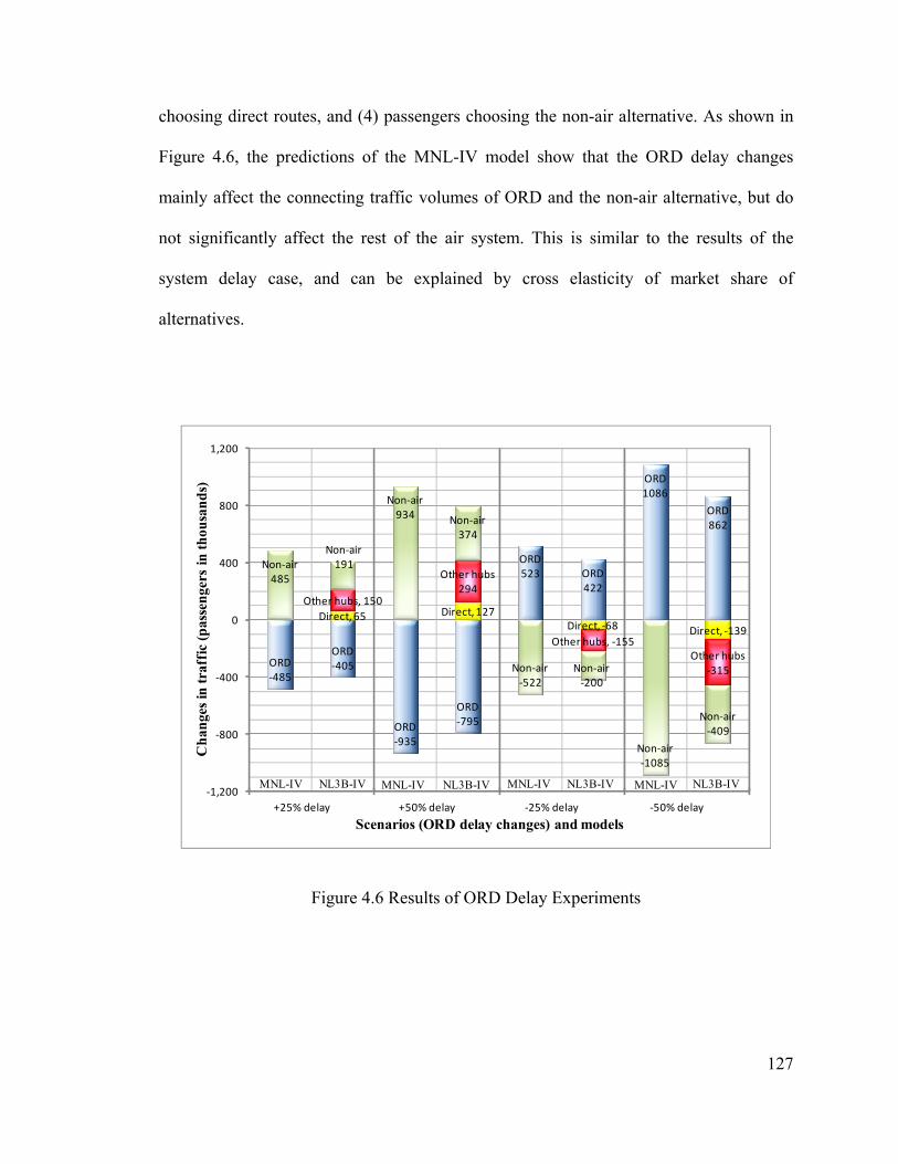
choosing direct routes, and (4) passengers choosing the non-air alternative. As shown in
Figure 4.6, the predictions of the MNL-IV model show that the ORD delay changes
mainly affect the connecting traffic volumes of ORD and the non-air alternative, but do
not significantly affect the rest of the air system. This is similar to the results of the
system delay case, and can be explained by cross elasticity of market share of
alternatives.
Direct, 65 Direct, 127Direct, ‐68 Direct, ‐139
Other hubs, 150
Other hubs294
Other hubs, ‐155Other hubs
‐315
Non‐air485
Non‐air191
Non‐air934 Non‐air
374
Non‐air‐522
Non‐air‐200
Non‐air‐1085
Non‐air‐409
ORD‐485
ORD‐405
ORD‐935
ORD‐795
ORD523 ORD
422
ORD1086
ORD862
‐1,200
‐800
‐400
0
400
800
1,200
+25% delay +50% delay ‐25% delay ‐50% delay
Cha
nges
in tr
affic
(pas
seng
ers
in th
ousa
nds)
Scenarios (ORD delay changes) and models
MNL-IV MNL-IVMNL-IVNL3B-IV NL3B-IVNL3B-IVNL3B-IVMNL-IV
Figure 4.6 Results of ORD Delay Experiments
127
128
On the other hand, the results from NL3B-IV model are more sensible: more than
half of the changes in ORD traffic volumes correspond to the traffic changes of other
hubs and/or direct routes. Changes in traffic volumes of other hubs are about 2.3 times
larger than those of direct routes. The routes with ORD as a connecting airport, thus, are
more likely to substitute for (or to be substituted by) other connecting routes than for (by)
direct routes. However, this substitution pattern is not due to nesting structures of models,
which do not differentiate connecting and direct routes. Rather main reason for this
substitution pattern is that for the majority of the markets associated with ORD, the total
market share of connecting routes in a market is larger than that of direct routes.
If a proposed project is expected to reduce the current delay of ORD by 25%, the
NL3B-IV model predicts an increase of 422 thousand connecting passengers (about 4.5%
of the original connecting volume) annually at ORD. The increased volume of traffic is
from three sources: (1) 68 thousand passengers change from direct routes to routes
connecting through ORD ; (2) about 155 thousand passengers are attracted from the other
29 hubs; and (3) 200 thousand passengers are from the potential travelers who chose
other modes or did not travel. From the viewpoint of the whole air system, the net effect
is an increase of 200 thousand passengers.
4.2.3 Summary and Discussions of Policy Experiments
As the policy experiments demonstrate different applications of the model, they
also show the importance of incorporating the non-air alternative in the model and the
more realistic substitution patterns of the NL model. Although both the MNL-IV and
NL3B-IV estimates may yield reasonable values-of-time and own- elasticities of demand,
129
only the NL3B-IV estimates provide sensible substitution patterns among alternatives. In
addition, empirical studies using MNL models without the non-air alternative may
overlook the unreasonable substitution patterns, because the market share differences
among alternatives are smaller than those of MNL models with the non-air alternative66.
The above policy experiments are conducted under the assumption that no routes
are generated (or eliminated) from these scenarios67. Thus, all substitutions are between
existing routes. This assumption may be reasonable (or cause fewer inaccuracies) for
short term planning purposes. For long term planning, the possibilities of network
changes should be taken into account. In such cases, predicted independent variables are
needed as the inputs for the model.
66 According to Equation (2.4), the substitution of alternatives in MNL models depends
on market shares of alternatives. Because the non-air alternative has a very large market share, compared to those of air routes, in each market, it more likely substitutes for air routes. As a result, the unreasonable substitution patterns are more likely to be observed if the non-air alternative is included in the choice set.
67 Additionally, in each scenario only one supply variable is changed, other supply variables, such as frequency, are unchanged.
130
4.3 Structural Changes over Time
In this section structural changes over time are investigated. As discussed in
chapter 3, fare and frequency are major determinants of air demand. Structural changes
related to these two factors, thus, are the focus of the investigation. In particular, the
hypothesis that fare sensitivity has increased and frequency sensitivity has (relatively)
decreased is tested. It is important to examine the stability of the structure of air travel
demand. For example, if the hypothesis is true but ignored, we may underestimate the
fare effects and overestimate the values of frequency. This may mislead about charge
schemes and investments on capacities.
Possible reasons for the structural changes over the data period (1995-2004)
include growth of e-commerce and emergence of low cost carriers. Rapid development of
the Internet and its applications may affect the structure of airline service demand since
they significantly increase availability of travel information and change ticket distribution.
The easy availability of travel information broadens potential travelers’ choice sets and
also helps potential travelers make better informed decisions. Potential travelers can, for
example, effortlessly compare many alternatives (different routes, airlines, fare, travel
time, etc.) side by side through a single website. Through conventional distribution
channels, such as travel agents, potential travelers may see less information and thus
consider fewer alternatives. For instance, potential travelers may not ask for cheaper
tickets if their agents already provide acceptable deals. Also, agent commission policies
sometimes created incentives for agents to sell more expensive fares.
131
The internet effects may lead to changes in observed travelers’ sensitivities to route
characteristics, since potential travelers can consider larger choice sets and do so more
knowledgeably than before. Sensitivity to fare is expected to increase, because the
majority of potential travelers search for low fares online and most internet-based
channels provide alternatives sorted by fare68—from low to high. Frequency, on the other
hand, plays a more important role in conventional channels, in which the passengers opt
for higher frequency options as a means of reducing search costs, than in internet-based
channels. Therefore, we expect fare sensitivity to have increased and frequency
sensitivity to have decreased over the data period.
Structural changes may also have resulted from the emergence of low cost carriers.
When potential travelers know that low cost carrier services are available, they may be
encouraged to search for lower fares. For example, they may consider alternative origin
and/or destination airports that are served by low cost carriers. The effects of low cost
carriers become larger when combined with the internet effects, due to lower search
costs.
4.3.1 Estimation Results and Discussion
In order to examine the structural changes of air demand, the preferred model
(NL3B-IV) is repeatedly estimated by using different annual data sets, which are subsets
68 Some online travel agents, such as Expedia, even provide fare alert services, which
may make potential travelers more sensitive to fare, and/or attract more price sensitive potential travelers.
of the original panel data set and are shorter panel (only four quarters) data sets. For
comparison purpose, the same procedure is implemented for the NL3B-OLS model. The
annual estimation results of the NL3B-OLS and the NL3B-IV models are presented in
Table 4.4 and Table 4.5, respectively. Note that the annual estimation of year 1995 is not
performed since the lag delay variables are specified in the models and the delay
variables of year 1994 are unavailable. Therefore, there are nine annual estimation results,
from column (1) to column (9) in each table. Estimation results of the whole panel data
set are also duplicated from Table 3.8 and added into column (10) of both tables for
comparison.
It is worth mentioning that the differences between two sets of annual estimates
(OLS vs. IV) are similar to those between the two whole panel estimates. For both annual
and panel estimates, the OLS method tends to lead to smaller (in absolute value) fare
coefficient(s) and larger ratio(s) of scale parameters ( ap λλ / ) than those from the IV
method. As discussed in section 3.4 and 4.1, while the estimates from the OLS method
imply unreasonable high VOTs, low (in absolute value) fare elasticities, and low
correlations between air routes, the estimates from the IV method suggest more sensible
VOTs, fare elasticities, and correlations. The IV estimates, therefore, are preferred and
further discussed.
132
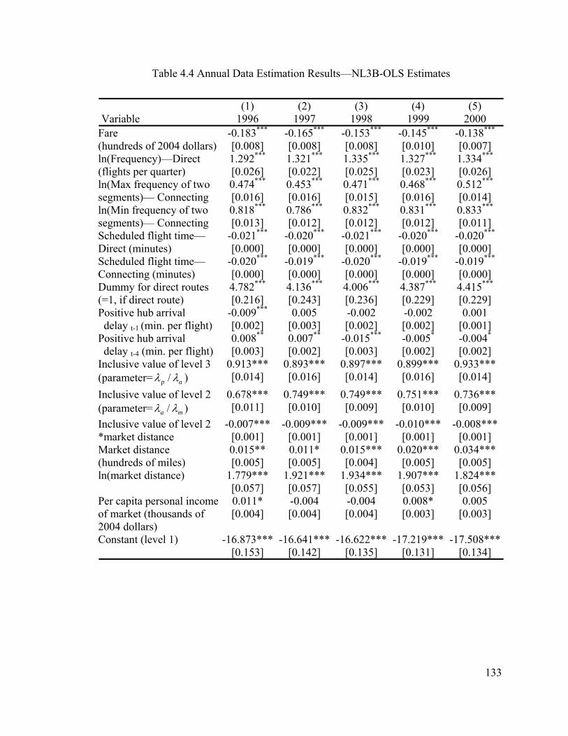
Table 4.4 Annual Data Estimation Results—NL3B-OLS Estimates
(1) (2) (3) (4) (5) Variable 1996 1997 1998 1999 2000
Fare (hundreds of 2004 dollars)
-0.183*** -0.165*** -0.153*** -0.145*** -0.138*** [0.008] [0.008] [0.008] [0.010] [0.007]
ln(Frequency)—Direct (flights per quarter)
1.292*** 1.321*** 1.335*** 1.327*** 1.334*** [0.026] [0.022] [0.025] [0.023] [0.026]
ln(Max frequency of two segments)— Connecting
0.474*** 0.453*** 0.471*** 0.468*** 0.512*** [0.016] [0.016] [0.015] [0.016] [0.014]
ln(Min frequency of two segments)— Connecting
0.818*** 0.786*** 0.832*** 0.831*** 0.833*** [0.013] [0.012] [0.012] [0.012] [0.011]
Scheduled flight time— Direct (minutes)
-0.021*** -0.020*** -0.021*** -0.020*** -0.020*** [0.000] [0.000] [0.000] [0.000] [0.000]
Scheduled flight time— Connecting (minutes)
-0.020*** -0.019*** -0.020*** -0.019*** -0.019*** [0.000] [0.000] [0.000] [0.000] [0.000]
Dummy for direct routes (=1, if direct route)
4.782*** 4.136*** 4.006*** 4.387*** 4.415*** [0.216] [0.243] [0.236] [0.229] [0.229]
Positive hub arrival delay t-1 (min. per flight)
-0.009*** 0.005 -0.002 -0.002 0.001 [0.002] [0.003] [0.002] [0.002] [0.001]
Positive hub arrival delay t-4 (min. per flight)
0.008** 0.007** -0.015*** -0.005* -0.004* [0.003] [0.002] [0.003] [0.002] [0.002]
Inclusive value of level 3 (parameter= ap λλ / )
0.913*** 0.893*** 0.897*** 0.899*** 0.933*** [0.014] [0.016] [0.014] [0.016] [0.014]
Inclusive value of level 2 (parameter= ma λλ / )
0.678*** 0.749*** 0.749*** 0.751*** 0.736*** [0.011] [0.010] [0.009] [0.010] [0.009]
Inclusive value of level 2 *market distance
-0.007*** -0.009*** -0.009*** -0.010*** -0.008*** [0.001] [0.001] [0.001] [0.001] [0.001]
Market distance (hundreds of miles)
0.015** 0.011* 0.015*** 0.020*** 0.034*** [0.005] [0.005] [0.004] [0.005] [0.005]
ln(market distance) 1.779*** 1.921*** 1.934*** 1.907*** 1.824*** [0.057] [0.057] [0.055] [0.053] [0.056]
Per capita personal income of market (thousands of 2004 dollars)
0.011* -0.004 -0.004 0.008* 0.005 [0.004] [0.004] [0.004] [0.003] [0.003]
Constant (level 1) -16.873*** -16.641*** -16.622*** -17.219*** -17.508***[0.153] [0.142] [0.135] [0.131] [0.134]
133
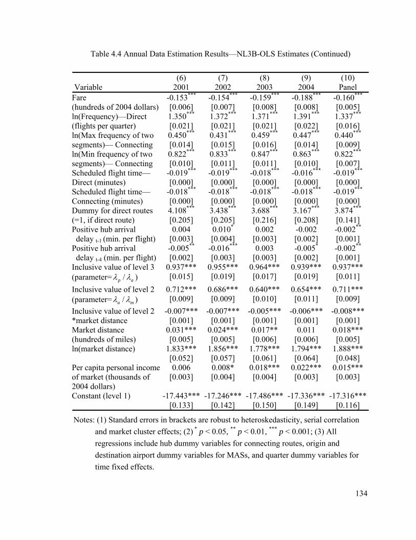
Table 4.4 Annual Data Estimation Results—NL3B-OLS Estimates (Continued)
(6) (7) (8) (9) (10) Variable 2001 2002 2003 2004 Panel
Fare (hundreds of 2004 dollars)
-0.153*** -0.154*** -0.159*** -0.188*** -0.160*** [0.006] [0.007] [0.008] [0.008] [0.005]
ln(Frequency)—Direct (flights per quarter)
1.350*** 1.372*** 1.371*** 1.391*** 1.337*** [0.021] [0.021] [0.021] [0.022] [0.016]
ln(Max frequency of two segments)— Connecting
0.450*** 0.431*** 0.459*** 0.447*** 0.440*** [0.014] [0.015] [0.016] [0.014] [0.009]
ln(Min frequency of two segments)— Connecting
0.822*** 0.833*** 0.847*** 0.863*** 0.822*** [0.010] [0.011] [0.011] [0.010] [0.007]
Scheduled flight time— Direct (minutes)
-0.019*** -0.019*** -0.018*** -0.016*** -0.019*** [0.000] [0.000] [0.000] [0.000] [0.000]
Scheduled flight time— Connecting (minutes)
-0.018*** -0.018*** -0.018*** -0.018*** -0.019*** [0.000] [0.000] [0.000] [0.000] [0.000]
Dummy for direct routes (=1, if direct route)
4.108*** 3.438*** 3.688*** 3.167*** 3.874*** [0.205] [0.205] [0.216] [0.208] [0.141]
Positive hub arrival delay t-1 (min. per flight)
0.004 0.010* 0.002 -0.002 -0.002** [0.003] [0.004] [0.003] [0.002] [0.001]
Positive hub arrival delay t-4 (min. per flight)
-0.005** -0.016*** 0.003 -0.005* -0.002** [0.002] [0.003] [0.003] [0.002] [0.001]
Inclusive value of level 3 (parameter= ap λλ / )
0.937*** 0.955*** 0.964*** 0.939*** 0.937*** [0.015] [0.019] [0.017] [0.019] [0.011]
Inclusive value of level 2 (parameter= ma λλ / )
0.712*** 0.686*** 0.640*** 0.654*** 0.711*** [0.009] [0.009] [0.010] [0.011] [0.009]
Inclusive value of level 2 *market distance
-0.007*** -0.007*** -0.005*** -0.006*** -0.008*** [0.001] [0.001] [0.001] [0.001] [0.001]
Market distance (hundreds of miles)
0.031*** 0.024*** 0.017** 0.011 0.018*** [0.005] [0.005] [0.006] [0.006] [0.005]
ln(market distance) 1.833*** 1.856*** 1.778*** 1.794*** 1.888*** [0.052] [0.057] [0.061] [0.064] [0.048]
Per capita personal income of market (thousands of 2004 dollars)
0.006 0.008* 0.018*** 0.022*** 0.015*** [0.003] [0.004] [0.004] [0.003] [0.003]
Constant (level 1) -17.443*** -17.246*** -17.486*** -17.336*** -17.316***[0.133] [0.142] [0.150] [0.149] [0.116]
Notes: (1) Standard errors in brackets are robust to heteroskedasticity, serial correlation and market cluster effects; (2) * p < 0.05, ** p < 0.01, *** p < 0.001; (3) All regressions include hub dummy variables for connecting routes, origin and destination airport dummy variables for MASs, and quarter dummy variables for time fixed effects.
134
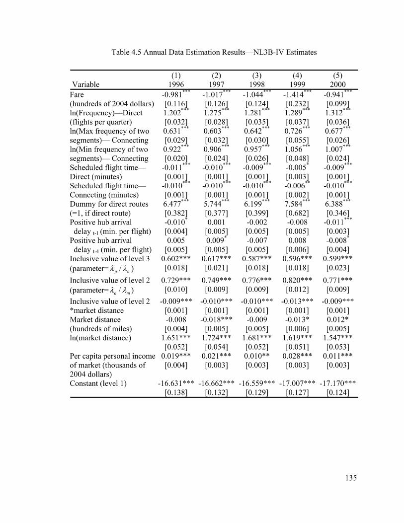
Table 4.5 Annual Data Estimation Results—NL3B-IV Estimates
(1) (2) (3) (4) (5) Variable 1996 1997 1998 1999 2000
Fare (hundreds of 2004 dollars)
-0.981*** -1.017*** -1.044*** -1.414*** -0.941*** [0.116] [0.126] [0.124] [0.232] [0.099]
ln(Frequency)—Direct (flights per quarter)
1.202*** 1.275*** 1.281*** 1.289*** 1.312*** [0.032] [0.028] [0.035] [0.037] [0.036]
ln(Max frequency of two segments)— Connecting
0.631*** 0.603*** 0.642*** 0.726*** 0.677*** [0.029] [0.032] [0.030] [0.055] [0.026]
ln(Min frequency of two segments)— Connecting
0.922*** 0.906*** 0.957*** 1.056*** 1.007*** [0.020] [0.024] [0.026] [0.048] [0.024]
Scheduled flight time— Direct (minutes)
-0.011*** -0.010*** -0.009*** -0.005* -0.009*** [0.001] [0.001] [0.001] [0.003] [0.001]
Scheduled flight time— Connecting (minutes)
-0.010*** -0.010*** -0.010*** -0.006** -0.010*** [0.001] [0.001] [0.001] [0.002] [0.001]
Dummy for direct routes (=1, if direct route)
6.477*** 5.744*** 6.199*** 7.584*** 6.388*** [0.382] [0.377] [0.399] [0.682] [0.346]
Positive hub arrival delay t-1 (min. per flight)
-0.010* 0.001 -0.002 -0.008 -0.011*** [0.004] [0.005] [0.005] [0.005] [0.003]
Positive hub arrival delay t-4 (min. per flight)
0.005 0.009* -0.007 0.008 -0.008* [0.005] [0.005] [0.005] [0.006] [0.004]
Inclusive value of level 3 (parameter= ap λλ / )
0.602*** 0.617*** 0.587*** 0.596*** 0.599*** [0.018] [0.021] [0.018] [0.018] [0.023]
Inclusive value of level 2 (parameter= ma λλ / )
0.729*** 0.749*** 0.776*** 0.820*** 0.771*** [0.010] [0.009] [0.009] [0.012] [0.009]
Inclusive value of level 2 *market distance
-0.009*** -0.010*** -0.010*** -0.013*** -0.009*** [0.001] [0.001] [0.001] [0.001] [0.001]
Market distance (hundreds of miles)
-0.008 -0.018*** -0.009 -0.013* 0.012* [0.004] [0.005] [0.005] [0.006] [0.005]
ln(market distance) 1.651*** 1.724*** 1.681*** 1.619*** 1.547*** [0.052] [0.054] [0.052] [0.051] [0.053]
Per capita personal income of market (thousands of 2004 dollars)
0.019*** 0.021*** 0.010** 0.028*** 0.011*** [0.004] [0.003] [0.003] [0.003] [0.003]
Constant (level 1) -16.631*** -16.662*** -16.559*** -17.007*** -17.170***[0.138] [0.132] [0.129] [0.127] [0.124]
135
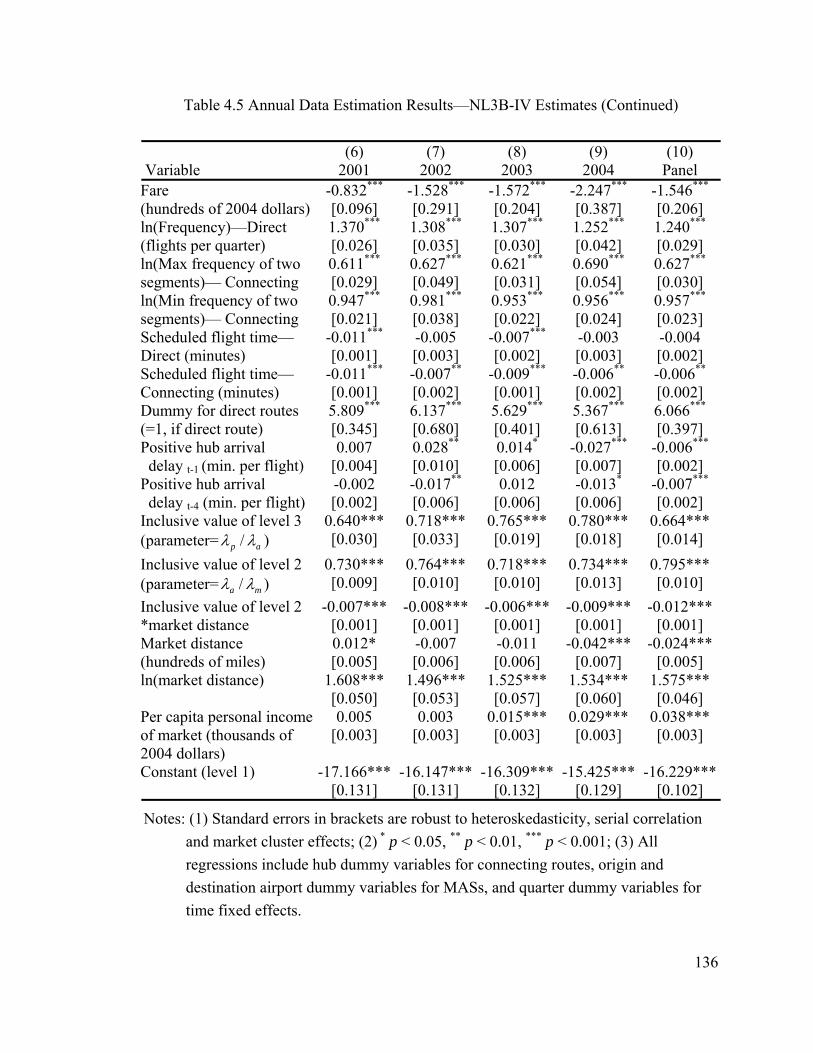
Table 4.5 Annual Data Estimation Results—NL3B-IV Estimates (Continued)
(6) (7) (8) (9) (10) Variable 2001 2002 2003 2004 Panel
Fare (hundreds of 2004 dollars)
-0.832*** -1.528*** -1.572*** -2.247*** -1.546*** [0.096] [0.291] [0.204] [0.387] [0.206]
ln(Frequency)—Direct (flights per quarter)
1.370*** 1.308*** 1.307*** 1.252*** 1.240*** [0.026] [0.035] [0.030] [0.042] [0.029]
ln(Max frequency of two segments)— Connecting
0.611*** 0.627*** 0.621*** 0.690*** 0.627*** [0.029] [0.049] [0.031] [0.054] [0.030]
ln(Min frequency of two segments)— Connecting
0.947*** 0.981*** 0.953*** 0.956*** 0.957*** [0.021] [0.038] [0.022] [0.024] [0.023]
Scheduled flight time— Direct (minutes)
-0.011*** -0.005 -0.007*** -0.003 -0.004 [0.001] [0.003] [0.002] [0.003] [0.002]
Scheduled flight time— Connecting (minutes)
-0.011*** -0.007** -0.009*** -0.006** -0.006** [0.001] [0.002] [0.001] [0.002] [0.002]
Dummy for direct routes (=1, if direct route)
5.809*** 6.137*** 5.629*** 5.367*** 6.066*** [0.345] [0.680] [0.401] [0.613] [0.397]
Positive hub arrival delay t-1 (min. per flight)
0.007 0.028** 0.014* -0.027*** -0.006*** [0.004] [0.010] [0.006] [0.007] [0.002]
Positive hub arrival delay t-4 (min. per flight)
-0.002 -0.017** 0.012 -0.013* -0.007*** [0.002] [0.006] [0.006] [0.006] [0.002]
Inclusive value of level 3 (parameter= ap λλ / )
0.640*** 0.718*** 0.765*** 0.780*** 0.664*** [0.030] [0.033] [0.019] [0.018] [0.014]
Inclusive value of level 2 (parameter= ma λλ / )
0.730*** 0.764*** 0.718*** 0.734*** 0.795*** [0.009] [0.010] [0.010] [0.013] [0.010]
Inclusive value of level 2 *market distance
-0.007*** -0.008*** -0.006*** -0.009*** -0.012*** [0.001] [0.001] [0.001] [0.001] [0.001]
Market distance (hundreds of miles)
0.012* -0.007 -0.011 -0.042*** -0.024*** [0.005] [0.006] [0.006] [0.007] [0.005]
ln(market distance) 1.608*** 1.496*** 1.525*** 1.534*** 1.575*** [0.050] [0.053] [0.057] [0.060] [0.046]
Per capita personal income of market (thousands of 2004 dollars)
0.005 0.003 0.015*** 0.029*** 0.038*** [0.003] [0.003] [0.003] [0.003] [0.003]
Constant (level 1) -17.166*** -16.147*** -16.309*** -15.425*** -16.229***[0.131] [0.131] [0.132] [0.129] [0.102]
Notes: (1) Standard errors in brackets are robust to heteroskedasticity, serial correlation and market cluster effects; (2) * p < 0.05, ** p < 0.01, *** p < 0.001; (3) All regressions include hub dummy variables for connecting routes, origin and destination airport dummy variables for MASs, and quarter dummy variables for time fixed effects.
136
137
As listed in Table 4.5, annual coefficients of the NL3B-IV model fluctuate over
time. However, direct comparisons between these coefficients may be inappropriate since
their values may be affected by scale parameters, which are also different over time.
Demand elasticities with respect to these variables and ratios of coefficients can be used
to describe the structural changes over time. Whereas no specific time trends for
scheduled flight time and market distance effects are found, structural changes related to
delay and income are apparent. Sensitivities to fare and frequency are further investigated
in the next section.
Only one-third (6 out of 18) of the estimated delay coefficients from the annual
data have the expected sign and significant different from zero, even though negative
delay impacts on route demand are confirmed by the whole panel data. More than half
(10 out of 18) of these coefficients are not significant. This indicates that delay effects are
mainly observed in a multi-year data set containing greater variation in delay. As shown
in Figure 4.7, the annual estimates of delay coefficients may be negative (such as the
results of year t-1 and t+1) or positive (e.g. the result of year t), and they may not
statistically significant. When there is enough variation, however, the negative delay
impact on route demand becomes apparent.
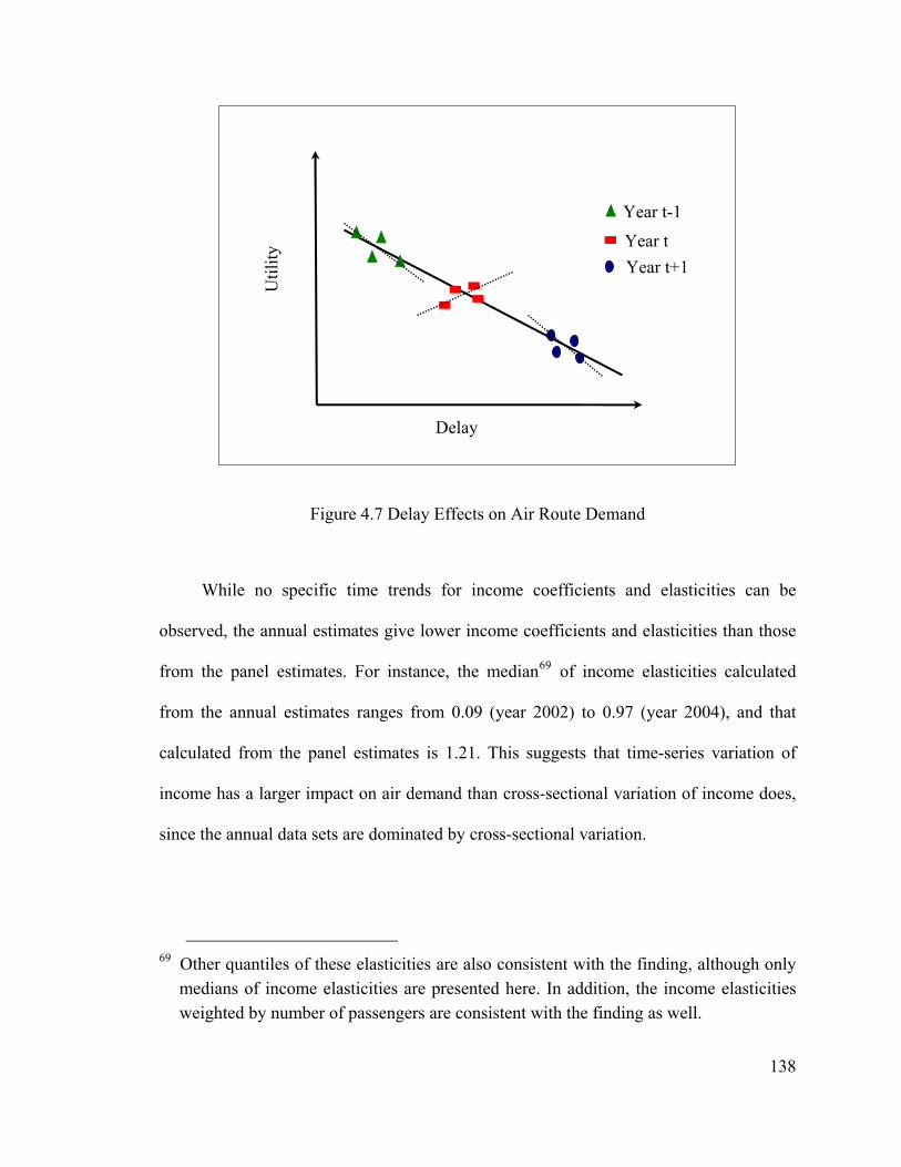
Year t+1 Year t
Util
ity
Delay
Year t-1
Figure 4.7 Delay Effects on Air Route Demand
While no specific time trends for income coefficients and elasticities can be
observed, the annual estimates give lower income coefficients and elasticities than those
from the panel estimates. For instance, the median69 of income elasticities calculated
from the annual estimates ranges from 0.09 (year 2002) to 0.97 (year 2004), and that
calculated from the panel estimates is 1.21. This suggests that time-series variation of
income has a larger impact on air demand than cross-sectional variation of income does,
since the annual data sets are dominated by cross-sectional variation.
138
69 Other quantiles of these elasticities are also consistent with the finding, although only
medians of income elasticities are presented here. In addition, the income elasticities weighted by number of passengers are consistent with the finding as well.
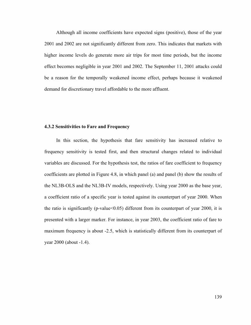
139
Although all income coefficients have expected signs (positive), those of the year
2001 and 2002 are not significantly different from zero. This indicates that markets with
higher income levels do generate more air trips for most time periods, but the income
effect becomes negligible in year 2001 and 2002. The September 11, 2001 attacks could
be a reason for the temporally weakened income effect, perhaps because it weakened
demand for discretionary travel affordable to the more affluent.
4.3.2 Sensitivities to Fare and Frequency
In this section, the hypothesis that fare sensitivity has increased relative to
frequency sensitivity is tested first, and then structural changes related to individual
variables are discussed. For the hypothesis test, the ratios of fare coefficient to frequency
coefficients are plotted in Figure 4.8, in which panel (a) and panel (b) show the results of
the NL3B-OLS and the NL3B-IV models, respectively. Using year 2000 as the base year,
a coefficient ratio of a specific year is tested against its counterpart of year 2000. When
the ratio is significantly (p-value<0.05) different from its counterpart of year 2000, it is
presented with a larger marker. For instance, in year 2003, the coefficient ratio of fare to
maximum frequency is about -2.5, which is statistically different from its counterpart of
year 2000 (about -1.4).
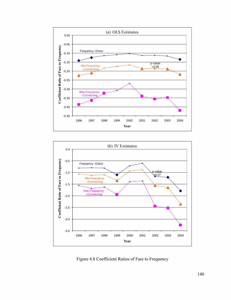
Frequency--Direct
Max Frequency--Connecting
p-value=0.06Min Frequency
--Connecting
-0.45
-0.40
-0.35
-0.30
-0.25
-0.20
-0.15
-0.10
-0.05
0.00
1996 1997 1998 1999 2000 2001 2002 2003 2004
Coe
ffic
ient
Rat
io o
f Far
e to
Fre
quen
cy
Year
(a) OLS Estimates
p-value=0.07
Frequency--Direct
Max Frequency--Connecting
Min Frequency--Connecting
-3.5
-3.0
-2.5
-2.0
-1.5
-1.0
-0.5
0.0
1996 1997 1998 1999 2000 2001 2002 2003 2004
Coe
ffic
ient
Rat
io o
f Far
e to
Fre
quen
cy
Year
(b) IV Estimates
Figure 4.8 Coefficient Ratios of Fare to Frequency
140
141
As shown in Figure 4.8, the ratios fluctuate over time, and the three ratios in the
same panel have similar patterns—they increase or decrease simultaneously, mainly
because the coefficients of frequency are more stable than those of fare. The OLS
estimates indicate that (1) the ratios increase first and then decrease after year 2000; (2)
the ratios of year 2004 are close to those of year 1996. Nevertheless, OLS estimates may
encounter the endogeneity problem of fare and as a result underestimate (in absolute
value) fare coefficients. The preferred IV estimates show that the ratios are stable before
year 2001, except for those of year 1999, and decrease after year 2001. That is, the
relative sensitivities do not significantly change in the earlier time periods, but do
increase in the later periods.
Although the results of OLS and IV estimates are inconsistent before year 2000,
they both suggest that fare sensitivity has increased relative to frequency sensitivity
starting in 2001. As discussed in the beginning of section 4.3, the sensitivity changes may
result from the effects of the Internet and low cost carriers. However, this research does
not further isolate these effects, leaving this for future research.
Structural changes related to each variable were further investigated by comparing
route demand elasticities with respect to these variables. Medians of these demand
elasticities from the preferred NL3B-IV estimates are plotted in Figure 4.9, from which
larger fluctuations of fare elasticities than those of frequency elasticities can be observed.
This is mainly because of the relatively stable frequency coefficients.
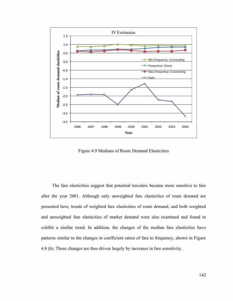
-3.5
-3.0
-2.5
-2.0
-1.5
-1.0
-0.5
0.0
0.5
1.0
1.5
1996 1997 1998 1999 2000 2001 2002 2003 2004
Med
ian
of r
oute
dem
and
elas
ticiti
es
Year
IV Estimates
Min Frequency--Connecting
Frequency--Direct
Max Frequency--Connecting
Fare
Figure 4.9 Medians of Route Demand Elasticities
The fare elasticities suggest that potential travelers became more sensitive to fare
after the year 2001. Although only unweighted fare elasticities of route demand are
presented here, trends of weighted fare elasticities of route demand, and both weighted
and unweighted fare elasticities of market demand were also examined and found to
exhibit a similar trend. In addition, the changes of the median fare elasticities have
patterns similar to the changes in coefficient ratios of fare to frequency, shown in Figure
4.8 (b). These changes are thus driven largely by increases in fare sensitivity.
142
143
Although frequency elasticities are relatively stable over time, an upward trend of
the demand elasticities with respect to frequency of direct routes can be observed. The
median grows from 0.62 (year 1996) to 0.84 (year 2004). This suggests that potential
travelers became more and more sensitive to frequency of direct routes over the study
period.
It is worth mentioning that although only median elasticities are presented here,
other quantiles and means of elasticities with respect to fare and frequency were also
checked. All the findings from the alternative elasticities are consistent with those from
the median elasticities.
144
Chapter 5 Conclusions and Recommendations
This chapter concludes this research by summarizing the methodological
contributions and empirical findings of the research. Moreover, recommendations for
future work are discussed.
5.1 Conclusions
By reviewing the literature on air travel demand, this research finds that current
understanding of the demand is lacking in several significant ways: (1) Most existing
models only deal with either demand generation or demand assignment, or apply these
two types of models sequentially; (2) The “induced” air travel is not captured by most
existing models; (3) How the relative importance of causal factors change over time is
seldom studied; (4) The pattern of correlations among different alternatives is not well
understood; and (5) Effects of on-time performance and market distance are
under-investigated. In order to fill the gaps, this research develops a city-pair air demand
model and applies it to the air transportation system of the United States. The main
methodological contributions and empirical findings are discussed below.
5.1.1 Methodological Contributions
The proposed model improves existing models by adding preferred features and
using an appropriate estimation method. The main methodological contributions are
listed as follows.
145
• The model can handle activities at a low aggregation level (route level), and can be
applied to a large network system. As demonstrated in chapter 3 and 4, the model is
applied to the air transportation system of the United States, and serves as a bottom-up
policy analysis tool for different scenarios. System impacts of changes in specific route
elements, such as airports or segments, can be evaluated.
• The model deals with demand generation and demand assignment in a single model,
and quantifies the “induced” air travel by adding a non-air alternative in the choice set.
Thus, a change in a causal factor, such as a fare increase, may influence both total air
demand and market shares of alternatives. With the non-air alternative, total air
demand is allowed to vary and potential travelers are not forced to choose one of the
air alternatives.
• Both multiple routes and multiple airport regions are considered in the model. This
leads to more complete choice sets, which are closer to what potential travelers can
choose from when they plan to travel between two cities.
• The model is able to investigate different patterns of correlations among alternatives.
• Using panel data, the model captures both time series and cross-sectional variation of
air travel demand. In addition, the stability of the structure of air travel demand is
examined. The panel data employed is publicly available and collected on a regular
basis so the model can be regularly updated.
• Effects of fare, frequency, scheduled flight time, direct routing, on-time performance,
income, and market distance on air demand are quantified. Demand elasticities with
respect to these causal factors are calculated.
146
• While most existing air demand models ignore the endogeneity problem of air fare, this
research applies the instrumental variables (IV) method to solve the problem. The
proposed instrumental variable for air fare is a cost side variable and is defined as the
product of the route distance and unit jet fuel cost.
5.1.2 Empirical Findings
Based on the results of chapter 3 and 4, main empirical findings, including model
forms, estimation methods, the assumption of saturated demand, effects of causal factors,
and structural changes over time, are summarized as follows.
Structure of Correlations for Airline Service Alternatives and Estimation Methods
The pattern of correlations among alternatives is explicitly captured by applying the
three-level nested logit (NL3B) model, which is the highest-level nested logit model
consistent with utility maximization. Other lower-level nested logit and multinomial logit
models are special cases of the NL3B model. The structure of the NL3B model implies
that a route is more likely to compete with another route of the same O-D airport pair
than the routes of the other O-D airport pairs, and is least likely to be substituted by the
non-air alternative.
The three-level nested logit model estimated by instrumental variable method
(NL3B-IV) is the preferred model for two reasons. First, the NL3B models confirm the
non-homogeneous correlations among alternatives, implying that the MNL models have
unreasonable substitution patterns among alternatives. Second, the IV estimates infer
more sensible values-of-time, demand elasticities, and correlations of total utilities for
147
alternatives than those of ordinary least squares (OLS) method. Due to endogeneity
problem, the fare coefficient estimated by OLS is biased towards zero. Thus, the inferred
fare elasticities and values-of-time are underestimated and overestimated, respectively. In
addition, the ratios of scale parameters estimated by OLS method are also biased. This
leads to unreasonable low correlations among air routes sharing the same O-D airport
pair.
As the policy experiments demonstrate different applications of the model, they
also numerically show the importance of incorporating the non-air alternative in the
model and the more realistic substitution patterns of NL model. Although both the
MNL-IV and NL3B-IV estimates yield reasonable values-of-time and own-elasticities of
demand, only the NL3B-IV estimates provide sensible substitution patterns among
alternatives.
Saturated Demand
In order to implement the proposed model, this research assumes that saturated
demand is 10 times the geometric mean of the city-pair population. Sensitivity tests of
this assumption confirm that the setting of the saturated demand only affect the estimated
intercept of the market share model if the proportionality factor is set large enough.
Fare
The empirical analysis suggests that air fare is endogenous and correcting the
endogeneity problem by the IV method significantly improves the fare coefficient and its
implications. The distributions of the fare elasticities (both of route and market demand)
clearly show that estimation methods (OLS versus IV) create much larger differences of
148
fare elasticities than model forms (MNL versus NL3B) do. In addition, for almost all
routes, whereas the unweighted fare elasticities from the OLS estimates suggest that route
demand is inelastic to fare, those from the IV estimates imply that route demand is fare
elastic. At market level, the fare elasticities from the OLS estimates indicate inelastic
market demand, but the unweighted fare elasticities from the IV estimates imply that for
the majority of markets (about 74% of markets according to the NL3B-IV estimates), air
demand is fare elastic.
The fare elasticities from the NL3B-IV estimates are better supported by findings in
the literature. As shown in Figure 4.2, the distributions of market demand elasticities
calculated from the NL3B-IV estimates and other studies—summarized by Gillen et al
(2002)—are very close, especially for larger absolute elasticities (smaller percentiles).
For example, the 1st quantile and median calculated from the NL3B-IV estimates are
-1.54 and -1.23, and those from Gillen et al (2002) are -1.52 and -1.15, respectively.
Flight Frequency
Although all estimated frequency coefficients indicate that potential travelers prefer
routes with high flight frequency, marginal effects of different frequency variables are
different. The results confirm the hypothesis that the minimum frequency is more critical
to the connecting service, and thus a proportional flight frequency increase on the
segment with lower frequency increases service attractiveness more than an equivalent
change on higher frequency segment.
149
Scheduled Flight Time
Although all coefficients of scheduled flight time indicate that travelers prefer
routes with shorter scheduled flight time, only the IV estimates suggest significantly
different marginal effects for different routing types. The IV estimates imply larger VOTs
for connecting routes than for direct routes. According to the NL3B-IV estimates, the
inferred values of scheduled flight time are $16.6/hour for direct routes and $24.1/hour
for connecting routes, both in 2004 dollars. These values are in the same order as those
reported in the literature. In addition, the elasticities calculated from the NL3B-IV
estimates suggest that shortening one percent of scheduled flight time is expected to
increase route demand by more than one percent for connecting routes, but less than one
percent for direct routes.
On-Time Performance
In IV estimations, positive hub arrival delay of one and four quarters before the
decision quarter are the only significant delay variables, although many on-time
performance metrics were tried. When choosing among connecting routes, travelers avoid
connecting at airports with high expected delay in certain seasons.
The coefficient differences between these two hub delay variables are not
statistically significant, implying that potential travelers weigh one-time performance of
the two periods equally. In addition, we expect that under steady state, a one-minute hub
delay increase has a larger impact on demand than an equivalent change in scheduled
flight time of a connecting route. The NL3B-IV estimates confirm this hypothesis: the
150
sum of two hub delay coefficients is larger than the coefficient of scheduled flight time
(both in absolute values).
Although hub arrival delay is statistically significant, it is relatively unimportant,
comparing to other causal factors. The elasticities of route demand with respect to hub
delay are much smaller in absolute values than elasticities with respect to other variables.
For example, the median elasticity with respect to hub delay of previous quarter is only
-0.056, according to the elasticities from the NL3B-IV estimates. Potential travelers will
not significantly benefit from delay improvements, unless the delay reductions are large.
According to our estimates, while positive hub delay reduces connecting route
attractiveness, negative delay has no effect. Moreover, even when potential travelers have
the chance of choosing O-D airports in MASs, on-time performance of these airports
does not notably affect their decisions, all else equal.
Income
The NL3B-IV estimates indicate air travel demand is strongly sensitive to income.
The quantiles of income elasticities from the NL3B-IV estimates—1.14 (1st quantile),
1.21 (median), and 1.29 (3rd quantile)—have a similar central tendency but less
dispersion compared to those of Gillen et al (2002)—0.81(1st quantile), 1.14 (median),
and 2.05 (3rd quantile). Particularly, almost all (more than 97% of markets; more than
99% of passengers) income elasticities from the NL3B-IV estimates are greater than 1,
implying that air demand is income elastic in most markets. In addition, income
elasticities have smaller variation across markets than fare and distance elasticities do.
151
Market Distance
On average, there is a concave relationship between market distance and air route
demand, controlling for other service variables. According to the NL3B-IV estimates, in
short- to medium-haul markets, the distance effects reflect declining competition from
competing modes, which causes air demand to increase with distance; in long-haul
markets, the effect is reversed, presumably due to decreasing propensity to travel.
Moreover, the estimated ratios of scale parameters from the NL3B-IV estimates imply
that in a longer-haul market route attribute changes are more likely to shift traffic
between routes as opposed to affecting total air market traffic.
Market distance effects for individual markets may vary since the NL3B model
allows markets with different service levels to have different distance effects. Market
demand elasticities with respect to market distance help understand the distance effects of
individual markets. While the majority of the distance elasticities from the NL3B-IV
estimates are positive, about 8% of markets (18% in terms of passenger traffic) have
negative demand elasticities with respect to market distance. This can be explained by the
concave relationship between market distance and total air demand.
Three main generalizations emerge from the analysis of distance elasticities. First,
for markets with distance less than 1200 miles, the longer distance market is expected to
have higher air demand, all else equal. Second, for markets with distance longer than
1200 miles, the percentage of markets (or passengers) with negative distance elasticities
increases with market distance. This indicates that declining propensity to travel has a
stronger impact of air traffic in longer-haul markets. Third, considering markets with
152
distance longer than 1200 miles, negative distance elasticities are more likely to be found
in higher traffic markets, which are usually better served and thus have larger inclusive
values. All else being equal, the influence of declining propensity to travel is more
pronounced in better served markets, while that of mode competition is stronger in minor
markets.
Structural Changes over Time
Whereas no specific time trends for scheduled flight time and market distance
effects are found, structural changes related to delay and income are apparent. Even
though negative delay impacts on route demand are confirmed by the whole panel data,
only one-third of the estimated delay coefficients from the annual data have the expected
sign and significant different from zero. This indicates that delay effects are mainly
observed in a multi-year data set containing greater variation in delay.
The annual estimates give lower income coefficients and elasticities than those
from the panel estimates. This suggests that time-series variation of income has a larger
impact on air demand than cross-sectional variation of income does. The annual income
coefficients indicate that markets with higher income levels do generate more air trips for
most time periods, but the income effect becomes negligible in year 2001 and 2002. The
September 11, 2001 attacks could be a reason for the temporarily weakened income
effect, perhaps because it weakened demand for discretionary travel affordable to the
more affluent.
The preferred NL3B-IV estimates show that fare sensitivity has increased relative
to frequency sensitivity starting in 2001. The changes of fare elasticities calculated from
153
NL3B-IV estimates show a similar pattern to the changes in coefficient ratios of fare to
frequency. These changes are thus driven largely by increases in fare sensitivity.
Although frequency elasticities calculated from NL3B-IV estimates are relatively stable
over time, an upward trend of the demand elasticities with respect to frequency of direct
routes can be observed. This suggests that potential travelers became more and more
sensitive to frequency of direct routes over the study period.
5.2 Recommendations
This research proposed a very general passenger demand model for air
transportation, which is presented in chapter 2. Nonetheless, to ensure tractability and due
to data constraints, assumptions and simplifications were made but may be relaxed in
future work. Potential improvements, including model forms, choice sets, data type, trip
stratifications, O-D airport-specific characteristics, and applications, are summarized as
follows.
Model Forms
In the empirical study, this research assumes that the saturated demand depends on
city-pair population. Although this approach yields satisfactory results, studies with
different purposes may need other approaches to calculate saturated demand. For
example, when the “large enough” proportionality factor is hard to decide for some
applications, or researchers are interested in the proportionality factor, other approaches
154
are needed. As discussed in chapter 2, one solution is to estimate a model for saturated
demand, although this increases the complexity of the model.
This research chooses the aggregate nested logit model for the market share
function in the empirical study, because (1) the empirical objective of this research
focuses on the coefficients and ratios of coefficients, and the nested logit model can serve
this purpose well, and (2) the nested logit model provides a good balance between
flexibility and computational complexity. Nevertheless, to recognize heterogeneity
among potential travelers and allow more flexible substitution patterns, the mixed logit
model may be considered, if the price of computational complexity is affordable. Refer to
section 2.2.3 for details of the mixed logit model and relevant literature.
Choice Sets
While possible transportation alternatives between two cities are included in the
choice set, the proposed model does not explicitly consider the cases that potential
travelers may choose other destination cities. This can be justified by two arguments.
First, the “outside good” alternative implicitly and partly captures these cases. Second,
“in air transportation there is little destination competition,” as described in Kanafani
(1983, p. 256). However, since characteristics of other cities are not specified in the
model, a characteristic change of a third city will not affect the demand between two
cities. In some applications, this may be problematic. For example, studies focusing on
vacation trips may need to capture the destination competition, since potential travelers
are not forced to go to a specific city for their vacations. Therefore, destination
competition should be kept in mind when we apply the proposed model. Adding
155
characteristics of other cities as explanatory variables and/or including destination
alternatives in the choice set can be solutions for this problem.
Another issue related to choice sets is that for simplicity, the proposed model does
not differentiate routes by carries. The model can be extended to the route-carrier level
when needed, although new nesting structures have to be examined, in order to model the
correlations among alternatives.
Data Type
This research chooses aggregate (at route level) data to estimate the model, because
the data is publicly available and collected on a regular basis. In some cases, disaggregate
data, which perhaps provides information closer to travelers’ behavior, may be available.
For example, individual fare information is available for the domestic markets of the
United States. However, the proposed model and estimation method need to be modified
to use disaggregate data.
Trip Stratifications
This research does not estimate different models for different categories of air trips
(for example, differentiating models by trip purposes). Since stratifying trips may better
explain travel behavior, it is worth estimating the proposed model by trip type—if
information is available.
O-D Airport-Specific Characteristics
In the empirical study, the origin and destination airport-specific characteristics,
which reflect attractiveness of airports in multiple airport systems, are mainly captured by
156
airport dummy variables. The estimated panel model assumes that the airport effects are
fixed over time, which may not be appropriate if airport characteristics significantly
change. Adding airport dummy variables for specific time periods may be able to solve
the problem. Another way is to explicitly specify airport-specific variables to capture
these effects. Although delay variables of O-D airports have been tried in this research,
they are not statistically significant. Other variables, particularly airport accessibility
variables, will improve our understanding of airport choice in multi-airport systems.
Applications of the Model
In addition to those applications shown in chapter 4, the proposed model can be
used to answer other interesting questions, such as (1) What are the specific effects of
Internet ticket distribution and low cost carrier growth on the structure of air demand? (2)
How does traveler welfare change under different charge schemes or delay reductions? (3)
Does the airport fixed effects change after a specific event?
As discussed in section 4.3, the sensitivity changes of fare and frequency may be
owing to the effects of the Internet and low cost carriers. However, this research does not
measure these effects directly due to data inavailability. When information on internet
usage (e.g. online ticket purchases over time) is available, it will be interesting to explore
these effects.
Although our policy experiments focused on the changes in traffic, they can be
extended to calculate traveler welfare changes under different charge schemes or delay
reductions.
157
Except for on-time performance metrics, this research assumes airport (as an origin,
destination, or connecting airport) effects are fixed over time in the panel model. It will
be interesting to further investigate these effects and trace their changes over time. For
example, a ground access improvement project, such as extending Bay Area Rapid
Transit (BART) service to San Francisco International Airport, may significantly change
the fixed effect of an airport. Quantifying these effects helps evaluate the project. The
proposed model is suitable for this kind of analysis.
158
References
Adler, Nicole, 2001. Competition in a deregulated air transportation market. European
Journal of Operational Research, Vol. 129, pp. 337-345.
Adler, Nicole, 2005. Hub-spoke network choice under competition with an application to
western europe. Transportation Science, Vol. 39, No. 1, pp. 58-72.
Adler, T, S. Falzarano, and G. Spitz Adler, 2005. Modeling service trade-offs in air
itinerary choices. Transportation Research Record: Journal of the Transportation
Research Board, No. 1915, pp. 20-26.
Ashford, N. and M. Benchemam, 1987. Passengers’ choice of airport: an application of
the multinomial logit model, Transportation Research Record, No. 1147, pp. 1-5.
Air Transport Association, 2005. Fuel cost and consumption
report. http://www.airlines.org/economics/energy/MonthlyJetFuel.htm. Accessed
April 27, 2005.
Basar, G., and C. R. Bhat, 2004. A parameterized consideration set model for airport
choice: An application to the San Francisco Bay area. Transportation Research Part
B, Vol. 38B, No. 10, pp. 889–904.
Ben-Akiva, M. and S. Lerman, 1985. Discrete choice analysis: Theory and application to
travel demand. Cambridge, MA: MIT Press.
Berry, S., 1994. Estimating discrete choice models of product differentiation. The RAND
Journal of Economics, Vol. 25, pp. 242-262.
159
tion=
Berry, S., J. Levinsohn, and A. Pakes, 1995. Automobile prices in market equilibrium.
Econometrica, Vol. 63, pp.841-890.
Brownstone, David, and Kenneth Train, 1999. Forecasting new product penetration with
flexible substitution patterns. Journal of Econometrics, Vol. 89, pp. 109-129.
Bureau of Economic Analysis, 2006. Local area personal
income. http://www.bea.gov/bea/regional/reis/default.cfm?catable=CA1-3&sec
2. Accessed July 11, 2006.
Bureau of Labor Statistics, 2008. Weekly and hourly earnings data from the current
population survey. http://data.bls.gov/cgi-bin/surveymost. Accessed March 20,
2008.
Coldren, G. M., F.S. Koppelman, K. Kasturirangan, and A. Mukherjee, 2003. Modeling
aggregate air travel itinerary shares: Logit model development at a major U.S.
airline, Journal of Air Transport Management, Vol. 9, No.6, pp.361-369.
Coldren, G.M. and F.S. Koppelman, 2005. Modeling the competition among air-travel
itinerary shares: GEV model development, Transportation Research Part A, Vol.
39A, No.4, pp. 345-365.
Corsi, T., M. Dresner and R. Windle, 1997. Air passenger forecasts: Principles and
practices. Journal of the Transportation Research Forum, Vol. 36, No. 2, pp. 42-62.
Data Base Products, 2004a. Hub and gateway training manual. Dallas, Texas.
Data Base Products, 2004b. Onboard domestic/ international operations manual—
Windows version. Dallas, Texas.
160
Data Base Products, 2005a. Hub 1995-2004 (CD-ROMs). Dallas, Texas.
Data Base Products, 2005b. Onboard domestic 1995-2004 (CD-ROMs). Dallas, Texas.
Data Base Products, 2007. The origin-destination survey of airline passenger traffic.
http://www.airlinedata.com/Documents/O&DSURV.htm. Accessed July 1, 2007.
De Vany, A. S. and E. H. Garges, 1972. A forecast of air travel and airport and airway
use in 1980. Transportation Research, Vol. 6, No. 1, pp. 1-18.
Dresner, M., J. C. Lin and R. Windle, 1996. The impact of low-cost carriers on airport
and route competition. Journal of Transport Economics and Policy, Vol. 30, No. 3,
pp. 309-328.
Dresner, M. and R. Windle, 1995. Are US air carriers to be feared? Implication of
hubbing to North Atlantic competition. Transport Policy, Vol. 2, pp. 195–202.
Federal Aviation Administration, 2001. Airport capacity benchmark report 2001.
Washington, D.C., USA.
Federal Aviation Administration, 2006. FAA long-range aerospace forecasts: Fiscal years
2020, 2025 and 2030. Washington, D.C., USA.
Federal Aviation Administration, 2007a. About airline service quality performance
(ASQP). http://aspm.faa.gov/information.asp . Accessed July 1, 2007.
Federal Aviation Administration, 2007b. Terminal area forecast summary: Fiscal years
2006-2025. Washington, D.C., USA.
Ghobrial, A., and A. Kanafani, 1995. Future of airline hubbed networks: Some policy
implications. Journal of Transportation Engineering, ASCE, Vol. 121, No. 2.
161
Gillen, D., W. Morrison, and C. Stewart, 2002. Air travel demand elasticities: Concepts,
issues and measurement. Final Report, Prepared for Department of Finance Canada.
Hansen, Mark, 1990. Airline competition in a hub-dominated environment: application
of non-cooperative game theory. Transportation Research Part B, Vol. 24B, No. 1,
pp. 27–43.
Hansen, Mark, 1995. Positive feedback model of multiple-airport system. ASCE Journal
of Transportation Engineering, Vol. 121, No. 6, pp. 453-460.
Hansen, Mark, 1996. Airline frequency and fare competition in a hub-dominated
environment. Unpublished paper.
Hansen, Mark, and Adib Kanafani, 1990. Airline hubbing and airport economics in the
pacific market. Transportation Research Part A, Vol. 24A, No. 3, pp. 217-230.
Hansen, Mark, and Tara Weidner, 1995. Multiple airport systems in the United States:
Current status and future prospects. Transportation Research Record: Journal of the
Transportation Research Board, No. 1506, Transportation Research Board of the
National Academies, Washington, D.C., pp. 8–17.
Harvey, G., 1987. Airport choice in a multiple airport region. Transportation Research
Part A, Vol. 21A, No. 6, pp. 439-449.
Hess, S., and J. W. Polak, 2005a. Mixed logit modelling of airport choice in multi-airport
regions. Journal of Air Transport Management, Vol. 11, No. 2, March 2005, pp.
59–68.
Hess, S., and J. W. Polak, 2005b. Accounting for random taste heterogeneity in airport
choice modeling. Transportation Research Record: Journal of the Transportation
162
Research Board, No. 1915, Transportation Research Board of the National
Academies, Washington, D.C., pp. 36–43.
Hess, Stephane and John W. Polak, 2006. Airport, airline and access mode choice in the
San Francisco Bay area. Papers in Regional Science, Vol. 85, No.4, pp. 543–567.
Hong, S., Harker, P.T., 1992. Air traffic network equilibrium: Toward frequency, price
and slot priority analysis. Transportation Research Part B, Vol. 26, No. 4, pp.
307-323.
Hsiao, Chieh-Yu, and Mark Hansen, 2005. Air transportation network flows: Equilibrium
model. Transportation Research Record: Journal of the Transportation Research
Board, No. 1915, Transportation Research Board of the National Academies,
Washington, D.C., pp. 12–19.
Hsu, C.-I., and Y.-H. Wen, 2003. Determining flight frequencies on an airline network
with demand-supply interactions. Transportation Research Part E, Vol. 39E, No. 6,
pp. 417–441.
Joint Planning and Development Office, 2004. Next generation air transportation system
integrated plan.
Joint Planning and Development Office, 2007. Concept of operations for the next
generation air transportation system, version 2.0.
Kanafani, Adib, 1983. Transportation demand analysis. New York: McGraw-Hill Book
Company.
163
Kanafani, Adib, Elisabeth Sadoulet, and Edward C. Sullivan, 1974. Demand analysis for
North Atlantic air travel. Berkeley: Institute of Transportation Studies, University of
California at Berkeley.
Kanafani, A. and S.L. Fan, 1974. Estimating the demand for short-haul air transport
system. Transportation Research Record, No. 526. Transportation Research Board
of the National Academies, Washington, D.C., pp. 1–15.
Kanafani, A. and A. Ghobrial, 1985. Airline hubbing: Some implications for airport
economics. Transportation Research Part A, Vol. 19A, No. 1, pp. 15–27.
Kanafani, A., G. Gosling, and S. Taghavi, 1977. Studies in the demand for short haul air
transportation. Special report. Institute of Transportation Studies, Berkeley.
McFadden, Daniel, 1978. Modeling the choice of residential location. In Spatial
Interaction Theory and Planning Models, edited by A. Karlgvist, et al. Amsterdam,
North-Holland.
McFadden, Daniel, 1981. Econometric models of probabilistic choice. In Structural
Analysis of Discrete Data, edited by C. Manski and D. McFadden, pp. 198-272.
Cambridge: MIT Press.
Morrison, Steven, and Clifford Winston, 1985. An econometric analysis of the demand
for intercity passenger transportation. Research in Transportation Economics,
Volume 2, edited by Theodore Keeler, pp. 213-237. JAI Press INC.
Metropolitan Transportation Commission, 2001. Regional airport system plan update
2000: final report.
164
Ndoh, N. N., D. E. Pitfield and R. E. Caves, 1990. Air transportation passenger route
choice: A nested multinomial logit analysis. In Spatial Choices and Processes, edited
by M. M. Fischer, P. Nijkamp and Y. Y. Papageorgiou, pp. 349-365. North-Holland:
Elsevier Science Publishers B.Y.
Nevo, Aviv, 1997. Demand for ready-to-eat cereal and its implications for price
competition, merger analysis, and valuation of new goods. Ph.D. Dissertation,
Harvard University.
Nevo, Aviv, 2001. Measuring market power in the ready-to-eat cereal industry.
Econometrica, Vol. 69, No.2, pp. 307-342.
Oum, T. H., D. W. Gillen, and S.E. Noble, 1986. Demands for fareclasses and pricing in
airline markets. Logistics and Transportation Review, Vol. 22, No. 3, pp. 195-222.
Oum, T. H., A. Zhang, and Y. Zhang, 1993. Inter-firm rivalry and firm-specific price
elasticities in deregulated airline markets. Journal of Transport Economics and
Policy, Vol. 27, No. 2, pp. 171-192.
Qum, T. H., W. G. Waters II, and J.S. Yong, 1992. Concepts of price elasticities of
transport demand and recent empirical estimates: An interpretative survey. Journal
of Transport Economics and Policy, Vol. 26, No. 2, pp. 139-54.
Pathomsiri, Somchai, and Ali Haghani, 1995. Taste variations in airport choice models.
Transportation Research Record: Journal of the Transportation Research Board, No.
1915, Transportation Research Board of the National Academies, Washington, D.C.,
pp. 27–35.
165
Pels E., P. Nijkamp, and P. Rietveld, 2001. Airport and airline choice in a multiple airport
region: An empirical analysis for the San Francisco Bay area, Regional Studies, Vol.
35, No.1, pp. 1-9.
Pels E., P. Nijkamp, and P. Rietveld, 2003. Access to and competition between airports:
A case study for the San Francisco Bay area. Transportation Research Part A, Vol.
37A, No. 1, pp. 71–83.
Quandt, Richard, and William Baumol, 1966. The demand for abstract transport modes:
Theory and measurement. Journal of Regional Science, Vol. 6, Issue 2, pp.13-26.
Ross, Alex, and Alison Swain, 2007. Fighting flight delay. Operations Research/
Management Science Today, April 2007.
Small, Kenneth, and Clifford Winston, 1999. The demand for transportation: Models and
applications. Essays in Transportation Economics and Policy: A Handbook in Honor
of John R Meyer. Brookings Institution Press, Washington, D.C., USA.
Train, Kenneth, 2003. Discrete choice methods with simulation, Cambridge University
Press.
U.S. Department of Transportation, 2001. Long distance transportation patterns: Mode by
trip distance. National Household Travel Survey, Washington, D.C., USA.
Warburg, V., C. Bhat, and T. Adler, 2006. Modeling demographic and unobserved
heterogeneity in air passengers' sensitivity to service attributes in itinerary choice.
Transportation Research Record: Journal of the Transportation Research Board, No.
1951, Transportation Research Board of the National Academies, Washington, D.C.,
pp. 7–16.
166
Wei, Wenbin, and Mark Hansen, 2005. Impact of aircraft size and seat availability on
airlines demand and market share in duopoly markets. Transportation Research Part
E, Vol.41E, No. 4, pp. 315–327.
Wei, Wenbin, and Mark Hansen, 2006. An aggregate demand model for air passenger
traffic in the hub-and-spoke network. Transportation Research Part A, Vol.40A, No.
10, pp. 841–851.
Weidner, T, 1996. Hubbing in U.S. air transportation system: Economic approach.
Transportation Research Record: Journal of the Transportation Research Board, No.
1562, Transportation Research Board of the National Academies, Washington, D.C.,
pp. 28–37.
Windle, R., and M. Dresner, 1995. Airport choice in multiple-airport regions, ASCE
Journal of Transportation Engineering, Vol. 121, No. 4, pp. 332-337.
Wooldridge, J. 2003. Introductory econometrics: A modern approach, 2nd edition.
Thomson.
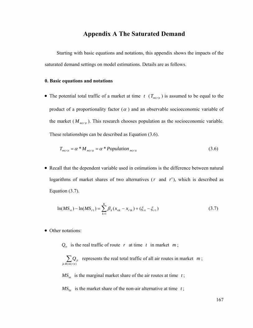
Appendix A The Saturated Demand
Starting with basic equations and notations, this appendix shows the impacts of the
saturated demand settings on model estimations. Details are as follows.
0. Basic equations and notations
• The potential total traffic of a market at time t ( trmT )( ) is assumed to be equal to the
product of a proportionality factor (α ) and an observable socioeconomic variable of
the market ( trmM )( ). This research chooses population as the socioeconomic variable.
These relationships can be described as Equation (3.6).
trmtrmtrm PopulationMT )( )()( ** αα == (3.6)
• Recall that the dependent variable used in estimations is the difference between natural
logarithms of market shares of two alternatives ( r and 'r ), which is described as
Equation (3.7).
)()()ln()ln( ''1
' trrttkr
K
krtkktrrt xxMSMS ξξβ −+−=− ∑
=
(3.7)
• Other notations:
rtQ is the real traffic of route r at time in market ; t m
∑∈ ))(( trmRj
jtQ represents the real total traffic of all air routes in market ; m
atMS is the marginal market share of the air routes at time ; t
tMS0 is the market share of the non-air alternative at time ; t
167
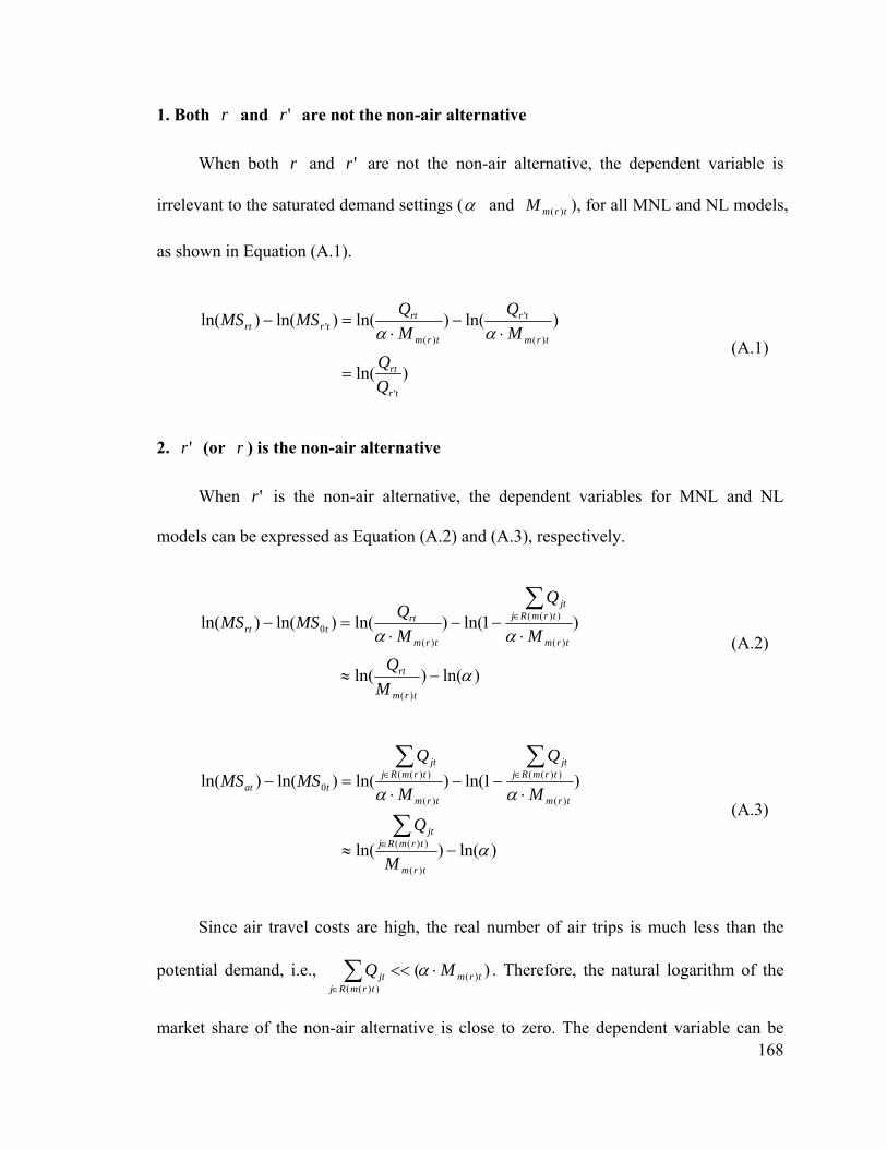
1. Both r and 'r are not the non-air alternative
When both r and 'r are not the non-air alternative, the dependent variable is
irrelevant to the saturated demand settings (α and ), for all MNL and NL models,
as shown in Equation (A.1).
trmM )(
)ln(
)ln()ln()ln()ln(
'
)(
'
)('
tr
rt
trm
tr
trm
rttrrt
MQ
MQMSMS
=
⋅−
⋅=−
αα (A.1)
2.
168
'r (or r ) is the non-air alternative
When 'r is the non-air alternative, the dependent variables for MNL and NL
models can be expressed as Equation (A.2) and (A.3), respectively.
)ln()ln(
)1ln()ln()ln()ln(
)(
)(
))((
)(0
α
αα
−≈
⋅−−
⋅=−
∑∈
trm
rt
trm
trmRjjt
trm
rttrt
MQ
M
Q
MQMSMS
(A.2)
)ln()ln(
)1ln()ln()ln()ln(
)(
))((
)(
))((
)(
))((0
α
αα
−≈
⋅−−
⋅=−
∑
∑∑
∈
∈∈
trm
trmRjjt
trm
trmRjjt
trm
trmRjjt
tat
M
Q
M
Q
M
QMSMS
(A.3)
Since air travel costs are high, the real number of air trips is much less than the
potential demand, i.e., . Therefore, the natural logarithm of the
market share of the non-air alternative is close to zero. The dependent variable can be
)( )())((
trmtrmRj
jt MQ ⋅<<∑∈
α
approximated by the second line of each equation, if the potential demand is set much
greater than the real total traffic. As shown in these approximated equations, different
proportionality factor (α ) settings are equivalent to adding different constant terms to the
dependent variables. Thus, the proportionality factor settings may only affect the
estimated intercept of the market share model if the proportionality factor is set large
enough. In addition, although population is not explicitly specified in the market share
function, it still helps to explain—through its impact on the calculation of market
shares—the market share variation between air routes and the non-air alternative, both
across markets and over time
Equations similar to (A.2) and (A.3) can be derived for the case that r is the
non-air alternative.
169
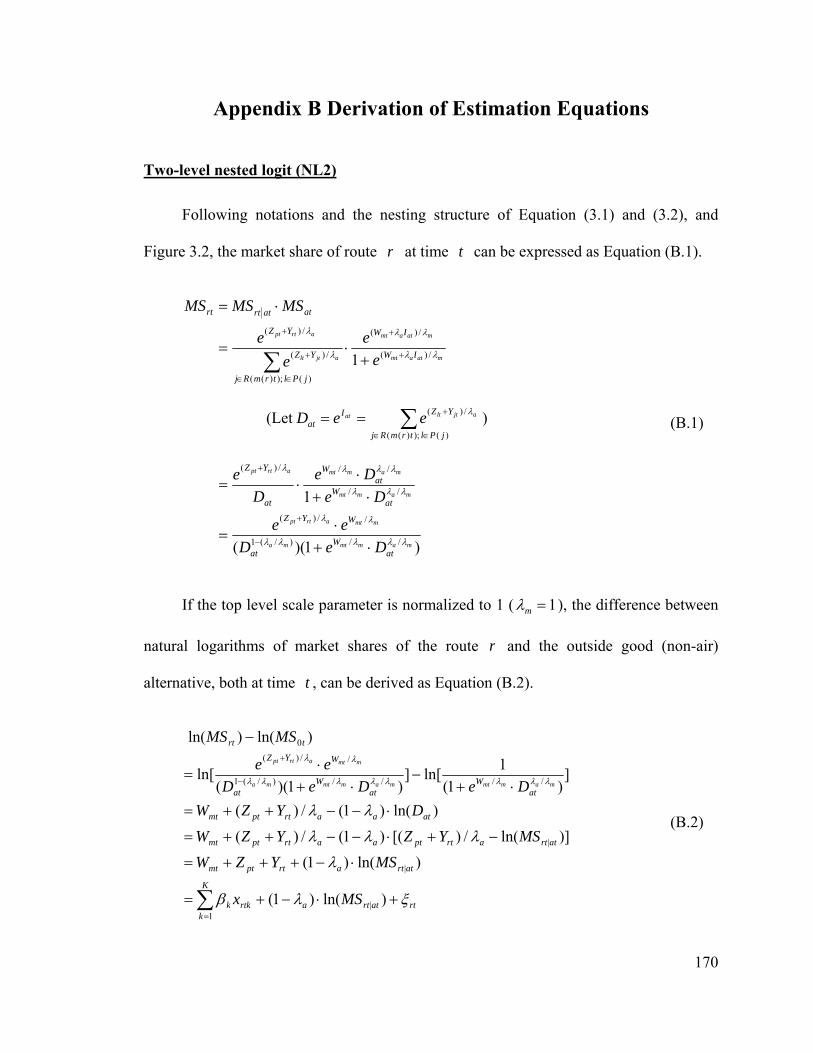
Appendix B Derivation of Estimation Equations
Two-level nested logit (NL2)
Following notations and the nesting structure of Equation (3.1) and (3.2), and
Figure 3.2, the market share of route r at time t can be expressed as Equation (B.1).
)1)((
1
1
//)/(1
//)(
//
///)(
/)(
/)(
)( );)((
/)(
/)(
mammtma
mmtartpt
mammt
mammtartpt
matamt
matamt
ajtlt
artpt
atW
at
WYZat
Wat
W
at
YZ
IW
IW
jPltrmRj
YZ
YZ
atatrtrt
DeDee
DeDe
De
ee
ee
MSMSMS
λλλλλ
λλ
λλλ
λλλλ
λλ
λλ
λ
λ
⋅+⋅
=
⋅+⋅
⋅=
+⋅=
⋅=
−
+
+
+
+
∈∈
+
+
∑
(B.1) (Let )( );)((
/)(∑∈∈
+==jPltrmRj
YZIat
ltat eeD λajt )
If the top level scale parameter is normalized to 1 ( 1=mλ ), the difference between
natural logarithms of market shares of the route r and the outside good (non-air)
alternative, both at time , can be derived as Equation (B.2). t
rtatrta
K
krtkk
atrtartptmt
atrtartptaartptmt
ataartptmt
atW
atW
at
WYZ
trt
MSx
MSYZW
MSYZYZW
DYZWDeDeD
ee
MSMS
mammtmammtma
mmtartpt
ξλβ
λ
λλλ
λλ
λλλλλλλλ
λλ
+⋅−+=
⋅−+++=
−+⋅−−++=
⋅−−++=⋅+
−⋅+
⋅=
−
∑=
−
+
)ln()1(
)ln()1(
)]ln(/)[()1(/)(
)ln()1(/)(
])1(
1ln[])1)((
ln[
)ln()ln(
|1
|
|
////)/(1
//)(
0
(B.2)
170
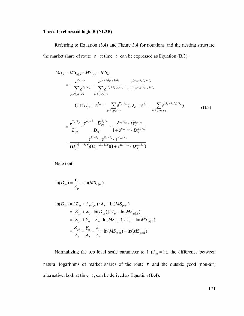
Three-level nested logit-B (NL3B)
Referring to Equation (3.4) and Figure 3.4 for notations and the nesting structure,
the market share of route r at time can be expressed as Equation (B.3). t
)1)()((
1
1
//)/(1)/(1
///
//
/////
/)(
/)(
))((
/)(
/)(
))((
/
/
mammtmaap
mmtaptprt
mammt
mammtapaptprt
matamt
matamt
altplt
aptppt
pjt
prt
atW
atpt
WZY
atW
atW
at
ptZ
pt
Y
IW
IW
trmPl
IZ
IZ
trpRj
Y
Y
atatptptrtrt
DeDDeee
DeDe
DDe
De
ee
ee
ee
MSMSMSMS
λλλλλλλ
λλλ
λλλ
λλλλλλλ
λλ
λλ
λλ
λλ
λ
λ
⋅+⋅⋅
=
⋅+⋅
⋅⋅
⋅=
+⋅⋅=
⋅⋅=
−−
+
+
∈
+
+
∈∑∑
(B.3)
171
Note that:
)ln()ln( |ptrtp
rtpt MSYD −=
λ
)ln()ln(
)ln(/)]ln([
)ln(/)]ln([)ln(/)()ln(
||
||
|
|
atptptrta
p
a
rt
a
pt
atptaptrtprtpt
atptaptppt
atptaptpptat
MSMSYZ
MSMSYZ
MSDZMSIZD
−⋅−+=
−⋅−+=
−⋅+=
−+=
λλ
λλ
λλ
λλ
λλ
Normalizing the top level scale parameter to 1 ( 1=mλ ), the difference between
natural logarithms of market shares of the route r and the outside good (non-air)
alternative, both at time , can be derived as Equation (B.4). t
)))((
; (Let /)(
))((
/ ∑∑∈
+
∈
====l
IZIat
trpRj
YIpt
atpjtpt eDeeD λλλ
trmP
altplte
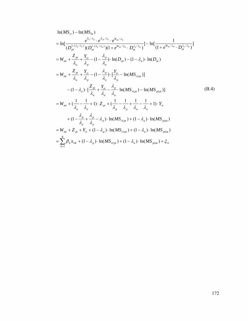
rtatptaptrtp
K
krtkk
atptaptrtprtptmt
atptaptrtpa
p
a
p
rtaapp
ptaa
mt
atptptrta
p
a
rt
a
pta
ptrtp
rt
a
p
p
rt
a
ptmt
atapta
p
p
rt
a
ptmt
atW
atW
atpt
WZYtrt
MSMSx
MSMSYZW
MSMS
YZW
MSMSYZ
MSYYZW
DDYZW
DeDeDDeee
MSMS
mammtmammtmaap
mmtaptprt
ξλλβ
λλ
λλλλ
λλ
λλλλλλ
λλ
λλλ
λλλ
λλ
λλλ
λλ
λλλλλλλλλλ
λλλ
+⋅−+⋅−+=
⋅−+⋅−+++=
⋅−+⋅−+−+
⋅+−+−+⋅+−+=
−⋅−+⋅−−
−⋅−−++=
⋅−−⋅−−++=
⋅+−
⋅+⋅⋅
=
−
∑=
−−
)ln()1( )ln()1(
)ln()1( )ln()1(
)ln()1()ln()1(
)11111()111(
)]ln()ln([)1(
)]ln([)1(
)ln()1()ln()1(
])1(
1ln[])1)()((
ln[
)ln()ln(
||1
||
||
||
|
////)/(1)/(1
///0
(B.4)
172