Party Polarization in Congress:

A Social Networks Approach

Andrew Scott Waugh, University of California, San DiegoLiuyi Pei, California Institute of Technology

James H. Fowler, University of California, San DiegoPeter J. Mucha, University of North Carolina at Chapel Hill

Mason A. Porter, University of Oxford

July 20, 2009

We use the network science concept of modularity to measure polarization in the United StatesCongress. As a measure of the relationship between intra-community and extra-community ties,modularity provides a conceptually-clear measure of polarization that directly reveals both the numberof relevant groups and the strength of their divisions. Moreover, unlike measures based on spatialmodels, modularity does not require predefined assumptions about the number of coalitions or parties,the shape of legislator utilities, or the structure of the party system. Importantly, modularity canbe used to measure polarization across all Congresses, including those without a clear party divide,thereby permitting the investigation of partisan polarization across a broader range of historicalcontexts. Using this novel measure of polarization, we show that party influence on Congressionalcommunities varies widely over time, especially in the Senate. We compare modularity to extantpolarization measures, noting that existing methods underestimate polarization in periods in whichparty structures are weak, leading to artificial exaggerations of the extremeness of the recent rise inpolarization. We show that modularity is a significant predictor of future majority party changes inthe House and Senate and that turnover is more prevalent at medium levels of modularity. We utilizetwo individual-level variables, which we call “divisiveness” and “solidarity”, from modularity andshow that they are significant predictors of reelection success for individual House members, helpingto explain why partially-polarized Congresses are less stable. Our results suggest that modularitycan serve as an early-warning signal of changing group dynamics, which are reflected only later bychanges in formal party labels.

1 Introduction

A great deal of recent research on Congress has been devoted to partisan polarization (McCarty,

Poole & Rosenthal 1997, Herrnson 2004, Jacobson 2004, Fiorina, Abrams & Pope 2005, Jacobson

2006, McCarty, Poole & Rosenthal 2007, Zhang, Friend, Traud, Porter, Fowler & Mucha 2008) and

1

the influence of party on roll-call voting (Rohde 1991, Cox & McCubbins 1993, Snyder & Groseclose

2000, McCarty, Poole & Rosenthal 2001, Cox & Poole 2002, Cox & McCubbins 2005, Smith 2007).

With few exceptions, such research has suggested that party leaders are able to successfully influence

the voting behavior of legislators, that this influence has resulted in increased partisan polarization

in Congress over the past 20 years (following a period of party decline), and that polarization in

Congress has increased polarization in the electorate (Jacobson 2000, Jacobson 2005).

However, this wealth of attention has resulted in few concrete measures of partisan polariza-

tion. In fact, nearly all studies of Congressional polarization rely on a single measure, which was

developed by McCarty, Poole, and Rosenthal (MPR) (2007) using DW-Nominate scores (Poole

& Rosenthal 1997, Poole 2005). DW-Nominate, a multi-dimensional scaling technique (Borg &

Groenen 1997), was designed to measure the ideological positions of individual legislators. It has

been successfully applied to study party influence in Congress, but it relies on a number of assump-

tions about the nature of the party system and the preferences of individual legislators. Although

these assumptions might have value in estimating the ideal preferences of individual legislators, it

is unclear whether they are appropriate for measuring a Congress-level phenomenon such as po-

larization. In particular, the assumption of a party-system structure constrains the MPR analysis

to the current Democratic-Republican two party system. By construction, this makes it difficult

to use such methods to investigate the ebb and flow of polarization over the course of American

history.

Here we use methods from network science to reconceptualize polarization. Suppose each leg-

islator is a “node” in the network and the similarity in their roll-call voting behavior indicates the

strength of a “tie” between them. In a highly-polarized legislature, indivals in groups like parties

have very strong ties within the groups but very weak ties between them. For example, in the

extreme case of pure party-line voting, all members of the same party are perfectly similar and

therefore have the strongest possible ties between each other. They also have the weakest possible

ties to members of the other parties. In contrast, individuals in a legislature with low polariza-

tion tend to have ties both to their own group and to other groups, reducing the gap between

within-group and between-group tie strength. In a legislature completely free of party-line voting,

2

individuals are just as likely to vote with members of the other party as with members of their

own.

Network scientists have recently developed a measure called “modularity” (Newman & Girvan

2004, Newman 2006a) that uses information about the ties between each pair of individuals in a

network to compare the strength of ties within each group to those between each group. “Modular”

networks contain groups that have many ties within them but few between them. Network analysts

call such groups “modules” or “communities” because they form strongly connected and cohesive

subnetworks that, in the extreme, are nearly separated from other parts of the network (Porter,

Onnela & Mucha 2009, Fortunato 2009). As the ties within groups become stronger and those

between groups become weaker, the network becomes more modular. Conceptually, this is exactly

what it means when one claims that groups are becoming more polarized. In a polarized legislature,

people stick to the party line and rarely cross the aisle.

An advantage of this new way of thinking about political polarization is that it also allows us

to quantify the number of cohesive groups or communities in a legislature and identify which

individuals belong to each group. Previous work has used similar procedures to study com-

munities formed by the network of legislative cosponsorships (Zhang et al. 2008), House com-

mittee memberships (Porter, Mucha, Newman & Warmbrand 2005, Porter, Mucha, Newman &

Friend 2007), and a large variety of other real-world and computer-generated networks (Porter,

Onnela & Mucha 2009, Fortunato 2009). Other applications of network analysis have also flowered

in the political science literature (see, e.g., Huckfeldt 1987, Fowler 2006a, Fowler 2006b, McClurg

2006, Baldassarri and Bearman 2007, Koger et al. 2009).

Unlike the MPR measure of polarization, modularity does not require any assumptions about

the structure of the party system or the nature of legislator preferences. Indeed, modularity can

be calculated for any assignment of nodes into groups in any specified network, allowing us to

measure polarization across the whole history of the U.S. Senate and House of Representatives. We

use community detection procedures to identify group assignments that maximize modularity for

each roll-call network for both the House and Senate in the 1st–109th Congresses and then compare

maximum modularity to the modularity that results when we assume that party membership defines

3

the relevant voting groups. Using this procedure, we can show the extent to which party divisions

drive polarization over time. Using regression analyses, we then find that maximum modularity is

a significant predictor of future majority party changes in both the House and the Senate.

By deriving group structures directly from the data rather than imposing them in the form

of an assumed party system, we observe communities as they exist based on behavior instead

of labels. With this methodology, we find several periods in American history—most notably,

during the 75th–95th Congresses from 1937 to 1979—in which a large discrepancy exists between

formal party divisions and real voting coalitions. We suggest that such discrepancies, and the

corresponding changes in maximum modularity, might serve as an early warning signal for changes

in the partisan composition of Congress. This is because community structure can reveal informal

changes in partisan alliances before they change formally through party labels. In order to test

this hypothesis, we use modularity values in Congress t to predict changes in the majority party

for Congressional term t + 1. We find a nonmonotonic relationship between modularity and the

stability of the majority party in both chambers of Congress. At low levels of modularity, there

is little impetus to coordinate a change in majority control, while at high levels there is little

the minority can do to overcome the majority’s cohesion. In both of these cases, majority status

changes are infrequent. However, at medium levels of modularity, there is a mix of impetus and

relaxed majority cohesion, yielding a party system that is significantly less stable. We call this the

“partial polarization hypothesis.”

Finally, our analysis helps to explain why partially-polarized Congresses exhibit the greatest

instability. First, modularity allows us to identify those legislators who are most polarizing (i.e., who

are most “divisive”) and those who align most closely with their group (which we call “solidarity”).

Second, we show using these ideas that divisiveness has a negative impact on individual reelection

chances but that the effect is mitigated for polarizing legislators who exhibit strong solidarity with

their group. This, then, yields instability in partially-polarized Congresses.

4

2 Modularity

2.1 Generating Adjacency Matrices

To measure modularity, the first step is to use roll-call votes to generate a network in the form of

an adjacency matrix (Wasserman & Faust 1994, Newman 2003) that describes voting similarities

among Congressmen. The roll-call (compiled by Keith Poole and Howard Rosenthal, 1997, 2007) for

a given two-year term of Congress is encoded in an n×b matrix, in which each element Mik equals 1

if legislator voted yea on bill k, −1 if he/she voted nay, and 0 otherwise. Because we are interested in

characterizing the affiliations between legislators (rather than those between legislators and bills),

we transform the voting matrix into an n × n adjacency matrix A, whose elements Aij ∈ [0, 1]

representing the extent of voting agreement between legislators i and j. We define these matrix

elements by

Aij =1bij

∑k

αijk , (1)

where αijk equals 1 if legislators i and j voted the same on bill k and 0 otherwise, and bij is the total

number of bills on which both legislators voted. Because the perfect similarity between a legislator

and herself provides no information, we set all diagonal elements to be zero (i.e., Aii = 0). The

matrix A thereby encodes a network of weighted ties between legislators, with weights determined

by the similarity of their roll-call records in a single two-year Congress.

We generated two types of adjacency networks for our study. In the first type, we use all

available roll-call votes (including unanimous and near-unanimous votes). This set of networks

thus makes no assumptions about the quality or content of lopsided roll-calls and lends conceptual

clarity to the resulting modularity calculations. In the second type, we follow the guidelines of

Poole & Rosenthal (1997) and consider only “non-unanimous” roll-call votes. A roll-call vote is

classified as “non-unanimous” if greater than 3% of legislators are in the minority. For modern

Congresses, this implies that a roll-call minority must contain at least 4 Senators or at least 13

Representatives to yield a “non-unanimous” vote. While we make no substantive claim about

the importance of dropping unanimous votes, we concentrate primarily on non-unanimous roll-

call adjacency matrices. This ensures that the data sets we analyze mirror those used by McCarty,

5

Poole, and Rosenthal (2007), permitting more explicit comparison of our polarization measure with

theirs.

2.2 Definition of Modularity

Having generated n×n networks of weighted connections between legislators, we can now calculate

modularity values for any partition of these graphs. Several software packages are available to

perform such calculations. In this paper, we use the igraph package developed by Gabor Csardi

and Tamas Nepusz (2006).

Modularity can be used to measure the quality of a given partition of a network into specified,

non-overlapping communities (Porter, Onnela & Mucha 2009, Fortunato 2009, Newman & Girvan

2004, Newman 2006a). Modularity relies on the intuitively-plausible notion that communities

within networks ought to consist of nodes with more intra-community ties than extra-community

ties (Newman & Girvan 2004, Newman 2006a). For a given network partition, the modularity Q

represents the fraction of total tie strength m contained within the specified communities minus

the expected total strength of such ties. The expected strength depends on an assumed null model.

Here we use the standard Newman-Girvan null model that posits a hypothetical network with the

same expected degree distribution as the observed network (Newman 2006a, Newman 2006b). One

can alternatively use other null models, such as ones that assume uniform connection probabilities

or signed ties (Traag & Bruggeman 2008).

The standard null model gives a modularity of

Q =1

2m

∑ij

[Aij −

kikj

2m

]δ(gi, gj) , (2)

where m = 12

∑i ki is the total strength of ties in the network, ki =

∑j Aij is the weighted degree

(i.e., the strength) of the ith node, gi is the community to which i belongs, and δ(gi, gj) = 1 if i

and j belong to the same community and 0 if they do not.

Large positive modularity values indicate that a given network partition has much stronger

intra-community tie strengths than would be expected by chance. In other words, the legislators

6

within the communities voted more often with each other than with legislators belonging to other

communities. This, in turns, indicates that a legislature is more polarized.

2.3 Modularity Maximization

Although one can calculate the modularity of any network partition, it is important for the purpose

of measuring the level of polarization in a given Congress to identify the partition that maximizes

the modularity (or, at minimum, one that nearly maximizes modularity). Because optimizing

modularity is an NP-complete problem (Brandes, Delling, Gaertler, Goerke, Hoefer, Nikoloski &

Wagner 2008), a number of computational heuristics have been developed (Danon, Diaz-Guilera,

Duch & Arenas 2005, Fortunato 2009, Porter, Onnela & Mucha 2009). In this paper, we use the

walktrap algorithm, which was developed by Pons and Latapy (2005) and has been implemented in

the R package igraph (Csardi & Nepusz 2006).1

The walktrap algorithm starts by partitioning the network into n communities, which each

contain a single node (i.e., a legislator). It calculates a measure of the distance between each

pair of communities and begins merging groups by taking short random walks between them,

operating under the principle that such walks should connect closely-tied nodes and identify relevant

communities. After each merging step, one calculates the modularity score for the current partition.

The algorithm finishes after n− 1 steps when the nodes have been merged into a single community

consisting of the full network. Although the algorithm always begins with n communities and

ends with a single community, it returns the maximum-modularity network partition that it was

able to find. The walktrap algorithm requires the user to specify the length of the random walk,

and Pons and Latapy (2005) recommend walks with 4 or 5 steps. However, we found that for

many Congresses, these lengths did not provide the maximum modularity score. To be thorough

in attempting to optimize modularity, we performed the walktrap algorithm 50 times for each

Congress (using random walks of lengths 1–50) and selected the network partition with the highest

modularity value from those 50. We will call this the “maximum modularity partition” (though,

strictly speaking, this cannot be proven to be the optimum without computationally-prohibitive1In practice, the fast greedy algorithm developed by Newman (2004), which is also implemented in igraph, recovers

nearly-identical partitions for almost every Congress, though other algorithms can identify different best partitions.

7

exhaustive enumeration (Brandes et al. 2008)).

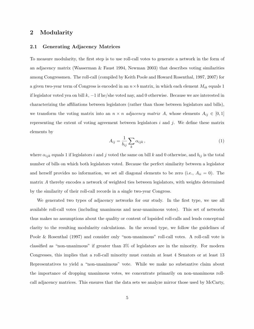
One can represent the results of the walktrap algorithm graphically (for a random walk of

specified length) in the form of a tree, or dendrogram, which shows the group mergers in a hier-

archical fashion and identifies communities of legislators who tend to cluster together. Horizontal

bars in such a plot are assigned a height depending on when they occurred in the algorithm (later

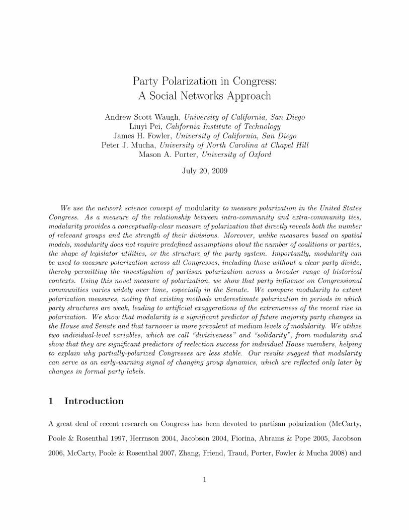
steps have a larger height). We show a dendrogram for the 75th Senate in Figure 1. This Senate,

which had an overwhelming Democratic supermajority (far exceeding the 2/3 majority necessary

at the time for a filibuster override) achieves its maximum modularity when partitioned into three

communities. The largest community (on the right) contains the majority of the Democrats and

some third-party Senators, the second-largest community (on the left) contains all of the Republi-

cans and 12 Democrats, and the smallest community (in the center) contains 10 Democrats and 1

Farmer-Labor member.

We found that for most Congresses, the maximum modularity occurs in a network partition

consisting of two communities, although several Congresses had a maximum-modularity partition

with three communities. Using only non-unanimous votes, the walktrap algorithm identified three

communities in Senates 2, 4, 13, 40, 41, 60, 63, 73, 75, and 77 and Houses 3, 17, 19, 43, 52, 74, 75,

81, and 98. Such three-community Congresses are rare, conforming to the expectation that single-

member districts tend to yield two-party systems (Duverger 1954, Cox 1997). Congresses with

three communities tend to occur when the party system is unstable and the maximum modularity

is low, suggesting that both modularity and three-community Congresses might be early indicators

of changes in the party-system structure. We explore this in more detail in Section 4.

3 Modularity as a Measure of Polarization

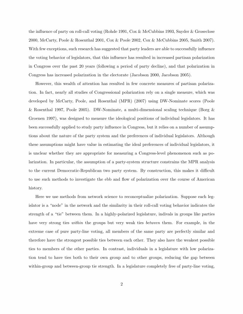
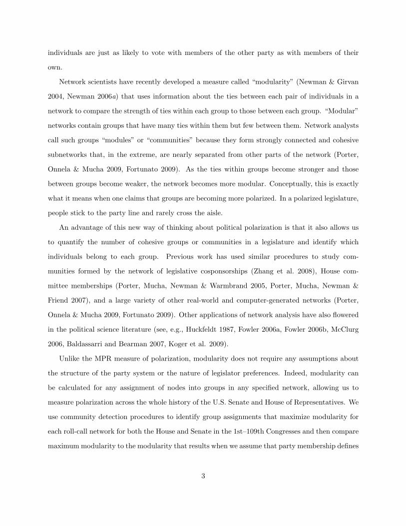
In Figures 2 and 3, we compare maximum modularity values to an existing polarization measure

that was introduced by McCarty, Poole, and Rosenthal (MPR) (1997, 2007). The MPR measure

is given by the absolute value of the difference between the mean first-dimension DW-Nominate

score (Poole 2005, Poole 2009) for members of one party and the same mean for the other party.

For comparability, we rescale both modularity and the MPR measure to lie in the range [0, 1].

8

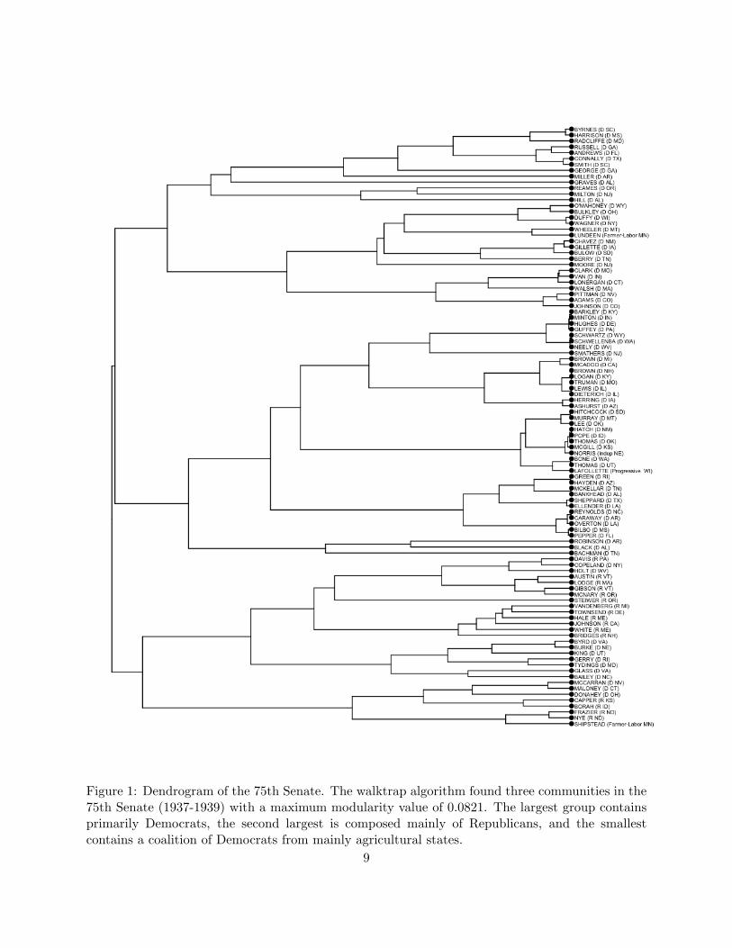
Figure 1: Dendrogram of the 75th Senate. The walktrap algorithm found three communities in the75th Senate (1937-1939) with a maximum modularity value of 0.0821. The largest group containsprimarily Democrats, the second largest is composed mainly of Republicans, and the smallestcontains a coalition of Democrats from mainly agricultural states.

9

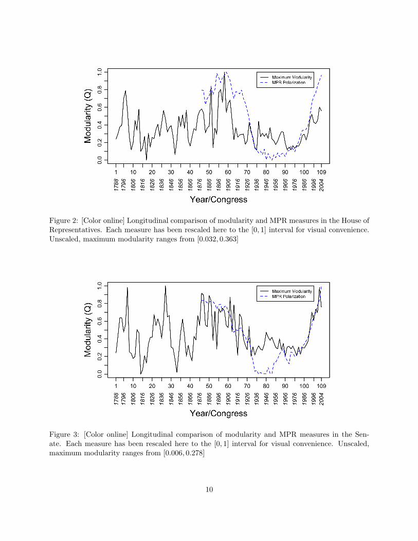
Figure 2: [Color online] Longitudinal comparison of modularity and MPR measures in the House ofRepresentatives. Each measure has been rescaled here to the [0, 1] interval for visual convenience.Unscaled, maximum modularity ranges from [0.032, 0.363]

Figure 3: [Color online] Longitudinal comparison of modularity and MPR measures in the Sen-ate. Each measure has been rescaled here to the [0, 1] interval for visual convenience. Unscaled,maximum modularity ranges from [0.006, 0.278]

10

Observe that unlike the modularity measure, the MPR measure assumes a competitive two-

party system (McCarty, Poole & Rosenthal 2007) and therefore cannot be calculated prior to the

46th Congress. Another difference is the year-to-year variance in the measure. MPR assumes

that legislators always remain in the same voting block and have fixed ideologies from year to year

(unless they switch parties), resulting in a time series that is smoother than that for the modularity

measure. In principle, one can achieve the same smoothness in the modularity measure using the

same assumptions, but as we discuss below, we believe that this variance is informative. Finally,

note that although the MPR and modularity measures both tell the same general story during the

46th–109th Congresses, the former suggests a much lower level of Congressional fractionalization

during the so-called ‘party decline’ era between the 75th–95th Congresses (Petrocik 1981, Ware

1985, Coleman 1996).

3.1 Comparison of Modularity and MPR Measures

The maximum modularity values in Figures 2 and 3 are consistent with several stylized facts about

polarization in Congress. Most notably, they capture the spike in fractionalization at the turn

of the 20th century caused by the end of Reconstruction and the recent spike in fractionalization

since the 95th Congress (Snyder & Groseclose 2000, McCarty, Poole & Rosenthal 2001, Cox &

Poole 2002, Jacobson 2004, Jacobson 2005, Jacobson 2006, McCarty, Poole & Rosenthal 2007,

Smith 2007, Zhang et al. 2008). The curves also show the lull in fractionalization that corresponds

to the party decline era during the 75th–95th Congresses (Petrocik 1981, Ware 1985, Coleman 1996).

By contrast, the MPR measure shows a much lower fractionalization during this period.

The period during the 75th–95th Congresses is one in which the maximum modularity differs

substantially from party modularity, which is simply the modularity of the network under the

assumption that legislators are assigned to groups that contain all of their fellow party members.

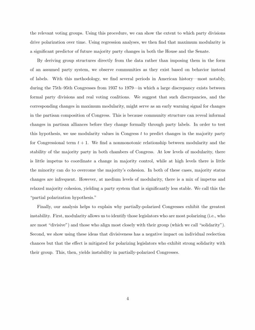
Figure 4 tracks the percentage 100 × P/Q of the maximum modularity value Q that is explained

by the party modularity value P . While maximum modularity measures the overall polarization

of a Congress, the percentage in Figure 4 indicates the relative contribution of party differences

to total polarization. The party partition captures the vast majority of the maximum modularity

11

in all modern Houses, with one notable exception consisting of the period during the 85th–95th

Congresses. Party importance varies more in the Senate, where it oscillates from one Congress to

the next between the 67th and 75th Congresses and is again a smaller part of maximum modularity

during the 85th–95th Congresses.

Figure 4: [Color online] Longitudinal plot of the percent of modularity explained by party for boththe House and Senate. The contribution of party to maximum modularity varies considerably overtime, particularly in the Senate.

Interestingly, although the MPR measure suggests substantially lower polarization than the

modularity measure for the 75th–95th Congresses, the party partition explains 90% or more of the

aggregate modularity for the 75th–84th Congresses before dropping to around 60% during the 85th–

95th Congresses. This result conveys the clearest difference in modern times between the MPR

measure and the modularity measure. The MPR measure suggests that party decline began around

the 70th Congress and continued until approximately the 90th, whereas the modularity measure—

particularly the proportion of modularity explained by party—suggest that the importance of party

did not start to wane until the 85th or 86th Congress. Notably, this is the only period in which

a fixed partition with three groups (Republicans, Southern Democrats, and Northern Democrats)

results in a higher modularity score than the normal two-party partition. These results suggest

12

that party was less important to Congressional fractionalization during the 75th–95th Congresses

than it was in other periods and that intra-party coalition tensions were generating heightened

polarization during this period that are not captured by the MPR measure.

This comparison yields at least two important substantive conclusions. First, the MPR un-

derestimation of polarization during the 75th–95th Congresses makes the subsequent rise in party

polarization seem more dramatic than that described by the modularity measure. This result likely

arises from the decision to calculate the MPR measure using only the first dimension of the DW-

Nominate scores. As Poole and Rosenthal identify, the second dimension of DW-Nominate, usually

attributed to civil rights issues, tends to explain a significant amount of variance in the roll-call

decisions of individual legislators over this period (1997). By creating an aggregate polarization

measure using only the first dimension, the MPR measure neglects this additional variance. In

contrast, the modularity measure avoids this problem because it does not require one to specify

dimensionality. As a result, it captures important divisions within parties in Congress during the

party-decline era, as legislators sought to forge new coalitions that ultimately yielded the current,

highly-polarized party system. Second, when viewed longitudinally, the MPR measure derives much

of its visual impact from its limitation to post-Reconstruction Congresses. The modularity measure

shows that modern-day polarization is high but not to a greater extent than in many other periods.

In fact, taking the entire history of Congress into account, it is the low-modularity period of the

75th–95th Congresses that appears to be the exception rather than the rule.

4 Modularity as a Predictor of Changes in Majority Status

4.1 Changes in Group Dynamics

The modularity-maximization algorithm generates both a community structure and a measure of

the strength of that structure that can be compared to the strengths of alternate groupings such

as parties, caucuses, and committees. Modularity gives us the opportunity to measure the gap

between stated political allegiances and actual political behavior. We chart this gap in Figure

4, which demonstrates the proportion of maximum modularity that can be attributed to party

13

divisions.

The existence of such a disparity is unsurprising. We do not expect legislators to be perfect

partisan agents, and we know that group dynamics have shifted and that the parties have reor-

ganized themselves several times in United States history (Burnham 1970, Merrill III, Grofman &

Brunell 2008). The most prominent partisan realignments have been captured in numerous longi-

tudinal studies of public opinion and voting behavior. These realignments represent changes in the

formal allegiances of Members of Congress. We assume that such changes are costly to politicians

and are thus unlikely to be undertaken without prior exhaustive effort to salvage the existing party

order. As a result, we expect informal tensions within parties to arise before formal changes occur.

As party bonds disintegrate, some legislators seek to preserve dying alliances while other, op-

portunistic legislators seek new alliances that reflect (or perhaps help create) a different order

(Riker 1986). Measures of polarization based on DW-Nominate are ill-equipped to identify these

shifts for two reasons. First, such measures assume a party-system structure to orient their legis-

lator coordinates in space. Second, such measures are weighted dynamically, which constrains the

spatial movement of legislators over time: like pawns in chess, legislators start on one side of a space

or the other and DW-Nominate permits them to move in only one direction over the course of their

careers. This restricted movement is a technical necessity that allows one to identify ideal points

on a consistent spatial metric over time (Poole 2005). Substantively, Poole defends this constraint

by appealing to evidence of party switchers in Congress. Namely, many legislators have changed

parties over their careers, but none have ever changed back (Cox & Poole 2002, Poole 2005).

This defense is justifiable if exogenously-defined group structures, such as party, are sufficiently

fine-grained to capture group dynamics or if the aim is to measure differences between modern

Republicans and modern Democrats. However, to measure changes in informal group dynamics

that anticipate changes in formal group structures, a consistent measure of group structure and

strength is needed that does not assume a party system or prevent politicians from wavering in

their beliefs over time. Modularity provides such a metric.

A clear indicator of a formal power shift in Congress is a change in the majority party. When

majority status changes hands in Congress, it is normally the result of major political or economic

14

failure on the part of the previous majority, reflecting the fact that voters no longer feel comfortable

with that party maintaining institutional control. One important way for a majority party to remain

effective is for its caucus members to coordinate on policy, as reflected in roll-call votes. The House

and Senate majorities resolve their coordination problems through various institutional means, such

as the delegation of agenda control to leaders and the appointment of party whips (Rohde 1991, Cox

& McCubbins 1993, Aldrich 1995, Cox & McCubbins 2005). However, the willingness of caucus

members to coordinate depends on a variety of forces, including electoral pressure, ideological

cohesion, and career ambition (Aldrich & Rohde 2001, Jacobson 2004).

If party membership is personally costly, then members might hedge their bets by seeking new

voting coalitions—either within their party or in other parties. Such fractures are captured in

the modularity-maximizing group structure by the emergence of third groups or the replacement

of party-dominated communities by more heterogeneously mixed groups. However, the effect of

such changes on the maximum modularity can be be quite variable, depending significantly on

the strength of the outgoing majority party. For example, the majority party in a low-modularity

Congress, in which group divisions are not particularly strong, might evolve into a more partisan

system, which leads to higher modularity scores. On the other hand, the majority in a high-

modularity Congress might suffer discontent that lowers aggregate modularity and leads to the

emergence of a less-partisan system.

As group structures in Congress evolve into forms that do not reflect party labels, interest

groups, party organizations, and ultimately voters begin to notice the gap, making the political

environment unstable. If these political actors support the party, then the legislator might be

replaced and the party system preserved. If, however, they support the legislator, then he or she

can either switch parties or attempt to drag the current party toward the policy preferences of his or

her district. If the legislator succeeds in moving the party, it will unsettle the electoral prospects of

fellow partisans in other districts. As a result, electoral volatility increases and changes in majority

status become more likely.

One empirical implication of this argument is that the modularity measure of the strength

of the group structure has the potential to yield predictive power over majority-party changes in

15

Congress. Below we perform a regression analysis that provides evidence that this is indeed the

case. To set the stage, we first offer a descriptive example of the ability of modularity to capture

changes in group dynamics before they are reflected in the formal party system.

4.2 A Descriptive Example from the 19th Century

As we discussed in Section 3, the modularity measure can be used to investigate party polarization

even during periods of history that include more than two dominant parties (i.e., before Recon-

struction). By construction, the MPR measure is not able to do this. Accordingly, we use the

modularity measure to consider an illustrative 19th century example.

In the early 19th century, the fledgling party system of the United States was going through a

transitional period. The existing party system, which pitted the dominant Democratic-Republicans

against a dying Federalist party, finally broke down in the 18th Congress (1823–1825) as the

Democratic-Republicans broke ranks based on their affiliations with national leaders, most notably

John Quincy Adams and Andrew Jackson. This resulted in a new period, reflected by partisan

conflict between supporters of Adams and supporters of Jackson, which lasted until the emergence

of the Whigs and the Democratic party in the 25th Congress (1837–1839) (Kernell, Jacobson &

Kousser 2009). The time series of the modularity measure captures this transition quite nicely

and provides evidence that group structures began to change as early as the 14th Congress, before

the Democratic-Republicans divided into the aforementioned camps. The Adams-Jackson party

system finally emerged in the 19th Congress, representing a change in majority party status in

both chambers.

One can see using modularity that the breakdown of the Democratic-Republican Party first

becomes apparent in the transition from the 13th to 14th Congress (i.e., with the 1814 election).

The second largest negative shift in modularity over the last 200 years occurs during this transition

in both chambers (−0.156 in the House and −0.127 in the Senate). This decline is particularly

interesting given that the country was experiencing a unified Democratic-Republican government

and that the Democratic-Republicans held huge majorities in both chambers. Some of this decline

is likely due to the end of the War of 1812 during the 13th Congress. With the war over, the

16

Democratic-Republicans no longer needed to maintain a united front, freeing individual Congress-

men or groups of Congressmen to pursue alternate agendas. In the Senate, this breakdown yielded

a maximum-modularity structure with three communities, suggesting that Democratic-Republicans

in the Senate were already beginning to explore alternate alliance structures.

In the House, this transition becomes further apparent in the 17th Congress (1821–1823), where

we again identify three communities when the Democratic-Republican party is nominally whole and

maintaining large majorities in both chambers of Congress. By the 18th Congress, the divisions

within the Democratic-Republican party become formally acknowedged, as three camps emerge

behind the leadership of Adams, Jackson, and William Crawford. This formal recognition results

in a dramatic increase in the maximum modularity of the House compared to the previous Congress,

demonstrating the impact that formal party divisions can have on legislator behavior. The same

basic groups had emerged during the 17th House, but had not yet formally consolidated into well-

defined camps. After this consolidation, however, the cost to coordinate had become lower, with an

accompanying increase in modularity and the elimination of the third community in the modularity-

maximizing structure. The elimination of the third community despite the emergence of a third

party is especially interesting, as it demonstrates that two of the parties saw the institutional value

in coordinating on roll-call votes in order to pursue their respective agendas in a majority-rule

institution. Thus, the modularity time series identifies the presence of a coalition government in

the 18th House. By the 19th House, however, the party system reforms into the pro-Adams and pro-

Jackson divisions. A change in majority status occurs, as the pro-Adams party assumes control of

both chambers. The House again achieves maximum modularity with three communities, suggesting

that the formal change in party label that had occurred was not yet salient to legislators. By the

20th Congress, however, a two-community partition emerges once more, and the House remains a

two-community body until the 43rd Congress (1873–1875), which took place during the throes of

Reconstruction.

We see from this anecdote that there is a lag between formal definitions of party and the

emergence of coalitions in Congress, and that this lag can work in both directions. In the 14th

Senate and 17th House, we identify three distinct communities in a period in which only two

17

parties nominally existed. When a three-party system becomes recognized in the 18th Congress,

modularity increases and the number of communities in the House reduces to two. Finally, when

a new two-party system becomes formalized in the 19th Congress, the House again devolves into

a three-community body. Modularity thus captures a fascinating distinction between the formal,

self-identifying claims of political parties and what coordinating activities are revealed by actual

voting behavior.

4.3 Data and Variables

We continue our analysis of group dynamics and polarization in Congress by conducting logistic

regression analyses. We compiled a time-series data set that covers each of the 4th–109th Con-

gresses.2 The data set contains both the key independent variable (maximum modularity) and the

key dependent variable (change in majority status) for each House and Senate. Change in majority

status is a binary variable that takes the value 1 if a switch occurred as a result of the previous

election and a 0 if it did not. Using information provided in Kernell et al. (2009), we identified

27 switches in the House and 26 switches in the Senate. We provide information about majority

status in Tables 4 (House) and 5 (Senate).

To control for the economic environment, we employed variables from historical data on rele-

vant economic indicators such as gross domestic product (GDP), consumer price index (CPI), and

national debt (as a percentage of GDP). These data can be found in the Historical Statistics of

the United States, Millennium Edition (2009). Additionally, we constructed a number of variables

representing particular structural features of the government. These include indicator (binary) vari-

ables for divided government, midterm Congress, and the presence of Republican or Democratic

majority. We included the first two variables to control for the impacts of presidents on electoral

outcomes, and we included the last two to capture any peculiar effects that a stable two-party

system has had on modularity or the likelihood of majority-party changes. Finally, we include an

indicator variable for Congresses that achieve maximum modularity with three communities, as

these Congresses are likely to be particularly unstable.2The accompanying economic data that we gather were not available for the earliest Congressional sessions.

18

4.4 Analysis

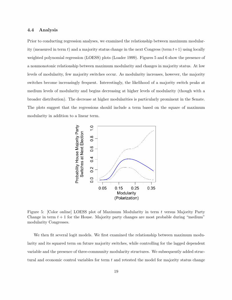
Prior to conducting regression analyses, we examined the relationship between maximum modular-

ity (measured in term t) and a majority status change in the next Congress (term t+1) using locally

weighted polynomial regression (LOESS) plots (Loader 1999). Figures 5 and 6 show the presence of

a nonmonotonic relationship between maximum modularity and changes in majority status. At low

levels of modularity, few majority switches occur. As modularity increases, however, the majority

switches become increasingly frequent. Interestingly, the likelihood of a majority switch peaks at

medium levels of modularity and begins decreasing at higher levels of modularity (though with a

broader distribution). The decrease at higher modularities is particularly prominent in the Senate.

The plots suggest that the regressions should include a term based on the square of maximum

modularity in addition to a linear term.

Figure 5: [Color online] LOESS plot of Maximum Modularity in term t versus Majority PartyChange in term t+ 1 for the House. Majority party changes are most probable during “medium”modularity Congresses.

We then fit several logit models. We first examined the relationship between maximum modu-

larity and its squared term on future majority switches, while controlling for the lagged dependent

variable and the presence of three-community modularity structures. We subsequently added struc-

tural and economic control variables for term t and retested the model for majority status change

19

Figure 6: [Color online] LOESS plot of Maximum Modularity in term t versus Majority PartyChange in term t+ 1 for the Senate. Majority party changes are most probable during “medium”modularity Congresses.

in the next term (t+ 1). We present our results in Table 1.

In all four model specifications summarized in Table 1, maximum modularity has a statistically

significant (p < 0.030)) positive impact on the probability of a change in majority party.

The squared term is significant (p < 0.048) and negative in both Senate specifications and the

first House specification, and it is negative and approaching significance (p ≈ 0.068) in the second

House model. None of the covariates are particularly important, although it is interesting to note

that increases in national debt as a percentage of GDP increases the likelihood of a switch in the

House, whereas increases in GDP itself increase the likelihood of a switch in the Senate.

We also compared the results from maximum modularity to results generated using the MPR

polarization measure (which is based on DW-Nominate). We show the results of these regressions

in Table 2. It appears from these results that the MPR measure is not a significant predictor of

changes in majority status. It should be noted, however, that the estimates for the MPR regression

cover only Congresses 46–109, as the MPR measure is not used to estimate polarization for earlier

Congresses.

The existence of a nonmonotonic relationship between modularity and changes in majority

20

House Senate(1) (2) (1) (2)

Max Modularity 52.78 (22.59) * 57.1 (26.3) * 54.27 (23.81) * 68.60 (27.4) *[Max Modularity]2 −115.77 (59.06) * −123.0 (67.4) . −165.10 (76.53) * −194.0 (86.0) *Three Communities 1.45 (0.93) 1.80 (1.08) . −15.9 (1210)Divided Government −0.91 (0.75) 0.16 (0.55)Midterm Congress −0.52 (0.56) 0.65 (0.54)2 year ∆GDP −1.22e−6 (3.19e−6) 4.94e−6 (2.33e−6) *2 year ∆CPI −0.36 (0.20) . −0.26 (0.16)2 year ∆Debt (% GDP) 46.7 (19.6) * 19.4 (14.6)Dem. Majority 0.01 (0.67) −0.17 (0.71)Rep. Majority −0.54 (0.72) −1.18 (0.73)Majority Change 0.39 (0.51) 0.94 (0.69) 0.54 (0.53) 0.50 (0.60)Intercept −6.34 (2.03) ** −6.29 (2.48) * −5.01 (1.71) ** −6.49 (2.16) **

Standard errors in parentheses. Significance codes (p <): *** 0.001, ** 0.01, * 0.05, . 0.1

Table 1: Logistic Regression Results. Majority party change in term t+ 1 modeled by variables interm t, with indicated standard errors and significance levels. Notably, the key independent variable,maximum modularity is significant in each model. Maximum modularity squared is significant inthree of the four models, and it almost reaching significance (p ≈ 0.068) in the other.

House SenateIntercept −1.89 (1.86) −2.12 (1.48)Majority Change 1.44 (1.04) 1.02 (0.69)MPR Polarization 1.97 (2.46) 0.55 (2.06)Divided Government −1.17 (1.12) 0.12 (0.73)Midterm Congress −1.18 (0.91) −0.02 (0.65)2 year ∆GDP −1.93e−6 (3.41e−6) 3.65e−6 (2.09e−6) .2 year ∆CPI −0.30 (0.22) −0.15 (0.13)2 year ∆Debt (% GDP) 46.94 (20.92) * 14.59 (13.80)

Standard errors in parentheses.Significance codes (p <): *** 0.001, ** 0.01, * 0.05, . 0.1

Table 2: Logistic Regression Results. Majority Party Change in term t+ 1 modeled by variables interm t, with indicated standard errors and significance levels. The key independent variable, MPRPolarization, appears to have no impact on majority party changes in the House or Senate.

21

status in Congress has important implications for the study of legislative organization and party

dynamics. It suggests, in particular, that partially-polarized Congresses experience the greatest

instability. This relationship might be driven by the strategic behavior of legislators, candidates,

and other partisans.

4.5 Discussion

The relationship between modularity and change in majority status is most easily explained by

dividing Congresses into three categories—those whose maximum-modularity partition has low,

medium, and high modularity scores. Recall that modularity quantifies the strength of the iden-

tified communities based on the relative number of intra-group connections versus extra-group

connections. We observe that low- and high-modularity Congresses tend to have stable majorities,

whereas the majorities in medium-modularity Congresses are less stable.

In low-modularity Congresses, group definitions are weak and (presumably) less salient to po-

litical actors. If one imagines Congressional activity as a coordination problem, low-modularity

Congresses are those in which coordination takes place between different coalitions on different is-

sues and in which mechanisms to aggregate preferences within groups have little power. In such an

environment, the transaction costs involved in collective action are likely to be very high—perhaps

high enough that individual legislators see little or no benefit in pursuing more permanent group

alliances. As in any collective action problem with high transaction costs, one danger is that individ-

uals will fail to act collectively and government will stagnate. Furthermore, the candidate-centered

electoral institutions of the United States (Herrnson 2004, Jacobson 2004) give individual legislators

a powerful incentive to pursue particular benefits for their districts in order to win reelection, even

at the expense of the public good. Any coordination that is accomplished likely occurs through

individual logrolling efforts, pork-barrel projects, and other exchanges of district-level benefits.

High-modularity Congresses have the opposite problem. In such Congresses, group structures

are well defined and usually party-oriented. Legislators in these Congresses have solved their coor-

dination problem by coalescing into stable voting blocs, which they use to achieve common goals.

However, individual legislators have less freedom to move across groups when group structures are

22

highly salient. Additionally, strong communities might be salient to members of the public as well

as fellow legislators. Thus, defecting from a well-established community might not only result in

ostracism from the group but might also be electorally costly. Donors, lobbyists, activists, and

other interested parties who have invested time and energy in the development of the existing

community structure might be less willing to support a legislator who has broken rank publicly.

Loss of active support from activists and elites, in turn, translates into a decreased probability of

reelection. We suspect that this pressure to conform drives the decrease in majority status changes

that we observe in high-modularity Congresses.

In contrast to both low- and high-modularity Congresses, medium-modularity Congresses reveal

environments that are in flux. These Congresses can take one of two forms: They either represent

a highly modular environment that is in the process of breaking down or a poorly-structured

environment in the process of consolidating. In such environments, when group structures exist

but are not well-established, opportunistic politicians have a clear incentive to act strategically

in an attempt to control the development of their communities. We suggest that conflict within

these coalescing or fracturing communities drives instability that occurs during medium-modularity

Congresses, as the communities frequently fracture and reconstitute themselves in the attempt to

settle on durable coalitions.

5 Divisiveness, Solidarity, and Reelection

Though the aggregate partisan stability of Congress over time generates interesting results and

suggests a general theory about the emergence and disintegration of legislative communities, it

does little to reveal the electoral prospects of individual legislators. As a Congress-level variable,

maximum modularity is too coarse to apply to legislator-level regressions, and it does not explain

why any particular legislator would win or lose an election. However, the group structure revealed

by the modularity-maximization process allows us to measure network attributes for each indi-

vidual within the communities. Here we elaborate two such measures: divisiveness, given by the

“community centrality” measure originally proposed by Newman (2006a), and solidarity, a measure

designed to explain how much an individual’s voting behavior aligns with his or her group’s voting

23

behavior.

5.1 Definition of Divisiveness and Solidarity

Mathematically, the divisiveness of legislator i is measured by the magnitude of a vector xi, which

is calculated through decomposition of the modularity matrix B, with components Bij = Aij− kikj

2m ,

from equation (2) into a set of eigenvalues, βj , and associated eigenvectors encoded as a matrix with

components Uij . From this decomposition, Newman (2006a) defines a set of vertex vectors {xi} of

dimension p, where p equals the number of positive eigenvalues of B. The magnitude |xi| of each

vertex vector measures the potential positive impact on aggregate modularity of each individual

legislator i. The vector magnitude is calculated using

|xi|2 =p∑

j=1

(√βjUij)2 (3)

(with the underlying definition of the vertex vectors given similarly by these components). The

divisiveness measure uses the roll-call adjacency matrices to estimate the potential effect that

each individual legislator has on the aggregate polarization of his or her body of Congress but

not necessarily the alignment of that legislator’s voting behavior to that of his or her own group.

Estimating alignment requires us to compare the divisiveness measure with the associated group

vector, obtained by summing over all vertex vectors corresponding to members of the group. This

is accomplished by calculating the solidarity, cos θik, where θik is the angle between the vertex

vector xi and the group vector Xk. When the solidarity is near 1, the legislator and community are

in strong alignment; on the other hand, when the solidarity is near 0, the legislator is not strongly

aligned with his or her community (Newman 2006a).

5.2 Divisiveness and the “Partial Polarization Hypothesis”

To examine the relationship between divisiveness, solidarity, and reelection, we begin with insights

derived from our analyses in Section 4.5 concerning the effect of modularity on changes in the

majority party in Congress. These results showed a nonmonotonic relationship between maximum

24

modularity and the survival of the majority party in Congress, with instability maximized at

medium levels of modularity. As we discussed above, this yields our partial polarization hypothesis.

We previously suggested that medium levels of modularity are unstable due to ongoing shifts in

the group structure of Congress, with some legislative alliances breaking down and others being

forged. We now wish to establish a connection between our Congress-level polarization measure

(i.e., modularity) and our individual-level divisiveness and solidarity measures. Although we use

majority party switches as a measure of political instability at the Congress level, at the legislator

level we are able to link modularity and divisiveness directly to reelection probabilities.

In Figure 7, we show a two-dimensional (2D) LOESS plot of the relationship between divisive-

ness, modularity, and the probability of a legislator being reelected. The contours of this graph

reveal a relationship between modularity and divisiveness as they interact to impact reelection.

Divisive Congressmen who serve in medium-modularity Congresses are the most likely to fail in

their reelection bids. However, in low-modularity Congresses and particularly in high modularity

Congresses, divisiveness appears to be a more successful strategy than in the medium-modularity

setting. We suspect that divisiveness in low-modularity Congresses remains successful because

group solidarity is less valuable in situations in which group structure is not salient. In high-

modularity Congresses, by contrast, we suspect that divisiveness is only successful in combination

with strong group solidarity, as groups are highly salient in these Congresses and members are

likely to be penalized for defecting from their groups. However, in medium-modularity Congresses,

when the structure and salience of groups is less clear, we suspect that Congressmen make more

errors in their voting decisions because of the more complicated legislative environment, resulting

in more reelection failures.

Teasing out the relationship between divisiveness, solidarity, and modularity requires us to

examine all three simultaneously. In Figure 8, we present a 2D LOESS plot that demonstrates

the relationship between divisiveness, solidarity, and modularity. This figure shows that high-

modularity Congresses are characterized by high levels of divisiveness and solidarity, implying that

groups are highly structured and polarized in these environments. Importantly, high modularity

is only sustained when both divisiveness and solidarity are high. If either divisiveness or solidarity

25

Figure 7: [Color online] Two-dimensional LOESS plot of Reelection versus Modularity and Di-visiveness. Color transitions from white to red as probability of reelection declines. The lowestreelection probabilities occur when divisiveness is high and modularity is at a “medium” level.

values dip, one observes a medium-modularity Congress. This suggests that instability in medium-

modularity Congresses might be driven either by divisiveness without solidarity or solidarity without

divisiveness. That is, in order for a group to be successful, it must be sufficiently divided from the

opposition (highly divisive) and internally cohesive (highly solidary).

Having associated (i) medium modularity and high divisiveness with decreased reelection proba-

bilities and (ii) high divisiveness and solidarity with high modularity, our final task is to demonstrate

the impact of solidarity and divisiveness on reelection probability. If the partial polarization hy-

pothesis is correct, we should observe that highly divisive Congressmen suffer in their electoral

prospects unless they also have high group solidarity. We demonstrate in Figure 9 that this is

indeed the case, particularly in the comparison between the middle right region and the upper

right corner. Combining this finding with the fact that Congressmen who exhibit high divisiveness

and low solidarity typically come from medium-modularity Congresses (recall Figure 8), we find

evidence of legislators struggling to forge new groups and sometimes failing. Many legislators in

medium-modularity Congresses appear to use votes to form coalitions (i.e., high divisiveness), but

when they fail to coalesce into cohesive groups (i.e., low solidarity), their divisiveness cannot be

26

Figure 8: [Color online] Two-dimensional LOESS plot of Maximum Modularity versus Divisivenessand Group Solidarity. Color transitions from red to white as maximum modularity increases. Thehighest levels of modularity occur only under conditions of high divisiveness and solidarity.

sustained and they are not reelected.

These figures suggest three hypotheses about the relationship between divisiveness, solidarity,

and reelection that would benefit from further statistical analysis in the presence of control variables.

First, increasing divisiveness causes a decrease in reelection probability. Second, increasing soli-

darity increases reelection chances. Finally, the impaired electoral probabilities of highly-divisive

legislators can be mitigated if their divisive behavior is consistent with the voting behavior of their

community. In other words, we expect a positive association between electoral probabilities and an

interaction between divisiveness and solidarity.

5.3 Data and Variables

We test our three hypotheses using a mixed-effects logistic regression specification on data from the

56th–103rd Houses of Representatives. We choose a mixed-effects specification because it allows

us to account for the fact that our data exist on multiple levels (Congress and legislator) and over

multiple time periods (56th–103rd Congresses). By including random effects for each legislator and

Congress, we are able to pool our data across time periods while still calculating accurate standard

27

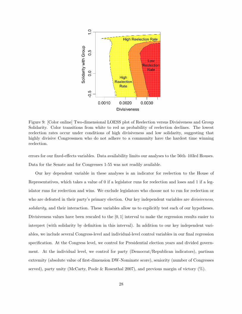
Figure 9: [Color online] Two-dimensional LOESS plot of Reelection versus Divisiveness and GroupSolidarity. Color transitions from white to red as probability of reelection declines. The lowestreelection rates occur under conditions of high divisiveness and low solidarity, suggesting thathighly divisive Congressmen who do not adhere to a community have the hardest time winningreelection.

errors for our fixed-effects variables. Data availability limits our analyses to the 56th–103rd Houses.

Data for the Senate and for Congresses 1-55 was not readily available.

Our key dependent variable in these analyses is an indicator for reelection to the House of

Representatives, which takes a value of 0 if a legislator runs for reelection and loses and 1 if a leg-

islator runs for reelection and wins. We exclude legislators who choose not to run for reelection or

who are defeated in their party’s primary election. Our key independent variables are divisiveness,

solidarity, and their interaction. These variables allow us to explicitly test each of our hypotheses.

Divisiveness values have been rescaled to the [0, 1] interval to make the regression results easier to

interpret (with solidarity by definition in this interval). In addition to our key independent vari-

ables, we include several Congress-level and individual-level control variables in our final regression

specification. At the Congress level, we control for Presidential election years and divided govern-

ment. At the individual level, we control for party (Democrat/Republican indicators), partisan

extremity (absolute value of first-dimension DW-Nominate score), seniority (number of Congresses

served), party unity (McCarty, Poole & Rosenthal 2007), and previous margin of victory (%).

28

5.4 Analysis

After selecting variables, we evaluated three mixed-effects logistic regression specifications. Unlike

our Congress-level regressions, in which we accounted for autocorrelation by including lagged depen-

dent variables, the data for these regressions are measured at two levels—Congress and legislator—

and then pooled over time. This data format, which is both cross-sectional and longitudinal,

necessitates a model that can appropriately estimate errors for our explanatory variables while ac-

counting for both Congress-level (across individuals) and individual-level (over multiple Congresses)

effects. The mixed-effects logistic regression model allows us to account for both Congress-level and

individual-level components as random effects by calculating random intercepts for these variables

(Gelman & Hill 2007). We draw the random intercepts from a Gaussian distribution with mean 0

and standard deviation equal to that of the variable. The functional form of the model resembles

a traditional logit with the random effects as additional parameters:

Pr(yi = 1) = logit−1(αlegislatori + αCongress

i + βfixedi + εi) . (4)

The first specification simply regresses divisiveness and solidarity against our reelection indica-

tor. The results in Table 3 show that divisiveness has a significant, negative impact on reelection

chances and that group solidarity has a positive impact. In the second specification, we include a

term that couples group solidarity and divisiveness.3 This model maintains the finding that divi-

siveness is associated with decreased reelection probability. It also shows that the combination of

divisiveness and solidarity has a strong positive impact on reelection, as indicated by the LOESS

plots. While the sign of solidarity flips from positive to negative, it is important to remember that

the total effect of solidarity must include the interaction term. At even moderately low levels of

divisiveness (starting around rescaled values of 0.2 or even lower), the effect of the interaction term

exceeds the main solidarity effect, suggesting that most legislators benefit from increased solidarity

with their community. Finally, the third specification reveals that the findings are robust to the3This interaction variable projects the vertex vector onto the group vector of its associated community, thereby

indicating the actual contribution to aggregate modularity made by assigning the legislator to that specific group(Newman 2006a)

29

(1) (2) (3)Divisiveness −4.548 (0.255) *** −15.873 (1.195) *** −17.261 (1.209) ***Solidarity 1.809 (0.196) *** −2.651 (0.513) *** −2.297 (0.535) ***Divisive×Solidarity 14.166 (1.453) *** 15.347 (1.463) ***Presidential Year −0.244 (0.202)Divided Government −0.351 (0.214)|Nominate (1st dim.)| 0.978 (0.240) ***Democrat −1.383 (0.423) **Republican −1.268 (0.423) **Seniority −0.069 (0.009) ***Party Unity −0.008 (0.002) ***Victory Margin 0.037 (0.001) ***Intercept 2.318 (0.194) *** 5.814 (0.424) *** 6.845 (0.620) ***

Fixed-effects coefficients. Standard errors in parentheses.Significance codes (p <): *** 0.001, ** 0.01, * 0.05, . 0.1

Random intercepts calculated at the Legislator and Congress levels.

Table 3: Mixed-Effects Logistic Regression Results for the 56th–103rd Houses. The dependentvariable is reelection to the House. The key independent variables are divisiveness, solidarity, andtheir interaction. Note that divisiveness and solidarity individually have a negative impact onelectoral prospects, but the interaction has a positive impact. This suggests that divisiveness mayonly be sustained by Congressmen who are also strong members of a community.

inclusion of common controls.

5.5 Discussion

The negative effect of divisiveness, which measures the potential for a Member of Congress to

increase the total modularity of a legislature, suggests that it is not beneficial to become too

involved in activities that create distinct voting blocs. Voters appear to penalize legislators whose

voting records most polarize the Congress. Simultaneously, legislators who show the most solidarity

with their communities appear to be protected from this penalty. It remains an open question for

future work how this process happens, but one possibility is that polarizing legislators inspire

enemies in other groups to work towards their defeat. Without the aid of a well-coordinated group,

a divisive legislator will not be reelected.

Our analysis suggests that voters are willing to accept divisiveness from their legislators, but

only to the extent that such divisiveness supports a strong group structure. It does not bode well

30

for reelection when a Congressmen is strongly aligned with a group but also violates acceptable

voting behavior for membership in that group. Conversely, Congressmen cannot be highly divisive

while simultaneously maintaining independence from a coalition. Only by appropriately balancing

group solidarity and individual divisiveness do Congressmen maximize their chances at reelection.

These individual-level results support the Congress-level findings and suggest that there are

indeed significant differences in the value of community attachment across different levels of po-

larization. In low-polarization environments characterized by the politics of logrolling and poorly-

organized leadership, being a member of a group is positive. However, being too strongly attached

to Congress as a whole is negative, suggesting that legislators in low-polarization environments are

expected by their constituents to pursue constituency interests first and foremost. (In this case, leg-

islators should recall Tip O’Neill’s adage that “All politics is local.”) However, in partially-polarized

Congresses, when group structures exist but are either not fully established or are breaking down,

legislators face a complex environment in which their choices about legislative alliance are subject

to greater error and thus greater risk. Nevertheless, in such environments, it can be beneficial to ef-

fectively balance commitments to community with other concerns. In highly-polarized Congresses,

the environment is more stable and the benefits and perils of alliance accrue primarily to those in

the largest community, though legislators with high divisiveness are still generally penalized unless

they are firmly embedded in their communities.

6 Conclusions

In this paper, we have presented a conceptually-clear measure of fractionalization and partisan

polarization in Congress using roll-call voting data and the network-science concept of graph mod-

ularity. We use computational heuristics to calculate the community structure that maximizes

modularity, thereby obtaining the membership and strength of communities in Congress. Because

calculating modularity requires no assumptions about the structure of the party system or the

nature of legislator preferences, we argue that it offers a clearer and more parsimonious measure

of polarization than the (MPR) measure based on DW-Nominate that currently dominates the

literature.

31

Unlike the measure based on DW-Nominate, the modularity-based measure can also be directly

applied to pre-Reconstruction Congresses, thereby allowing investigation of polarization across a

broader historical range. Here we investigated the quantitative similarities and differences between

the two measures and demonstrated that there exists a nonmonotonic relationship between modu-

larity and changes in the majority party in both chambers of Congress, which suggests that there

exists a level of polarization at which party instability is maximal. We further examine this “partial

polarization hypothesis” using two measures of community centrality—divisiveness and solidarity—

which capture the individual-level impacts of legislative alliances on reelection chances for House

members. Our results demonstrate the potential importance of the modularity-based polarization

measure and call for additional in-depth analyses of Congressional polarization.

The introduction of modularity and its allied concepts of divisiveness and solidarity to the

analysis of Congressional behavior has the potential to fundamentally alter the study of group

dynamics and partisanship in legislatures. Researchers have long sought to separate the effects of

party on voting behavior from electoral, interest group, and other pressures. These studies have

either assumed the existence of parties and their concomitant structure (Cox & McCubbins 1993,

Poole & Rosenthal 1997, McCarty, Poole & Rosenthal 2007) or assumed an alternate legislative

ordering mechanism such as committees (Shepsle 1979) or institutionally-derived pivotal members

(Krehbiel 1998, Tsebelis 2002), and then proceeded to make arguments about implications for the

structure of roll-call voting. Typically, in these cases, the organizational mechanism—be it parties,

committees, or veto pivots—is considered in isolation. Our results suggest that the complexities of

Congressional behavior are not captured by the implications of any particular idealized model of

legislative organization. Rather, by making simple assumptions about the nature of group strength,

we are able to partition Congressmen into groups while remaining agnostic about any particular

mechanism. We measure the strength of that group structure using modularity and the positioning

of legislators within that structure using divisiveness and solidarity.

By its nature, modularity cannot offer a causal link between community strength in Congress

t and majority party switch in Congress t + 1. However, it does provide a benchmark measure

of voting polarization against which to compare alternate legislative orderings. By comparing

32

the modularity values of party divisions, committee divisions, or other exogenously-determined

structures to the group structure revealed by modularity maximization, one might be able to

identify the environmental and strategic conditions under which particular organizational concepts

are likely to succeed and fail, allowing one to disentangle the complex interplay of environmental,

ideological, and institutional pressures that impact the structure of the Congressional voting record.

Furthermore, although the task of establishing such a causal mechanism is left to future research,

the strong correlation that our analysis reveals implies that this link takes place primarily in the

electoral arena. We hypothesize that the community structure of Congress in term t exerts a

strong influence on the behavior of donors, candidates, party organizations, and activists. It causes

them to strategically invest their energy either in preserving the existing order or in attempting to

create a new order. We suggest that the willingness of political opportunists to pursue a new order

depends on the presence of a community structure that is neither too strong to break nor too weak

to identify. In future work, we intend to gain traction on this problem by examining the impact

of modularity on the behavior of actors in Congressional elections. Meanwhile, we hope that other

scholars will build on the efforts presented herein and use network science to explore the dynamics

of coalition formation in the U. S. Congress and in other legislatures around the world.

7 Appendix: Changes in Majority Status

In this appendix, we present tables that summarize the changes in majority party in the House of

Representatives (in Table 4) and Senate (in Table 5).

33

Table 4: Changes in Majority Status in the House of Representatives.

34

Table 5: Changes in Majority Status in the Senate.

Acknowledgements

We obtained roll-call voting data from the voteview website (Poole 2009). We thank A. J. Friend,

Wojciech Gryc, Eric Kelsic, Keith Poole, Amanda Traud, Doug White, and Yan Zhang for useful

35

discussions. ASW, JHF, and MAP gratefully acknowledge a research award (#220020177) from

the James S. McDonnell Foundation. PJM’s participation was funded by the NSF (DMS-0645369).

References

Aldrich, John H. 1995. Why Parties? The Origin and Transformation of Political Parties in

America. Chicago: University of Chicago Press.

Aldrich, John H. & David W. Rohde. 2001. The Logic of Conditional Party Government. In

Congress Reconsidered, 7th Edition, ed. Lawrence C. Dodd & Bruce I. Oppenheimer. Wash-

ington D.C.: CQ Press.

Baldassarri, Delia & Peter Bearman. 2007. “Dynamics of Political Polarization.” American Socio-

logical Review 72:784–811.

Borg, Ingwer & Patrick Groenen. 1997. Modern Multidimensional Scaling: Theory and Applications.

New York: Springer-Verlag.

Brandes, Ulrik, Daniel Delling, Marco Gaertler, Robert Goerke, Martin Hoefer, Zoran Nikoloski &

Dorothea Wagner. 2008. “On modularity clustering.” IEEE Transactions on Knowledge and

Data Engineering 20(2):172–188.

Burnham, Walter Dean. 1970. Critical Elections and the Mainsprings of American Politics. New

York: Norton.

Coleman, John J. 1996. Party Decline in America. Princeton, NJ: Princeton University Press.

Cox, Gary W. 1997. Making Votes Count. Cambridge: Cambridge University Press.

Cox, Gary W. & Keith T. Poole. 2002. “On Measuring Partisanship in Roll-Call Voting: The U.S.

House of Representatives, 1877-1999.” American Journal of Political Science 46(3):477–489.

Cox, Gary W. & Mathew D. McCubbins. 1993. Legislative Leviathan: Party Government in the

House. Berkeley, CA: University of California Press.

36

Cox, Gary W. & Mathew D. McCubbins. 2005. Setting the Agenda: Responsible Party Government

in the U.S. House of Representatives. Cambridge: Cambridge University Press.

Csardi, Gabor & Tamas Nepusz. 2006. “The igraph software package for complex network research.”

InterJournal Complex Systems 1695.

Danon, Leon, Albert Diaz-Guilera, Jordi Duch & Alex Arenas. 2005. “Comparing community

structure identification.” Journal of Statistical Mechanics: Theory and Experiment (P09008).

Duverger, Maurice. 1954. Political Parties: Their Organization and Activity in the Modern State.

New York: Wiley.

Fiorina, Morris P., Samuel J. Abrams & Jeremy C. Pope. 2005. Culture War? The Myth of a

Polarized America. New York: Pearson Longman.

Fortunato, Santo. 2009. “Community detection in graphs.” arXiv:0906.0612.

Fowler, James H. 2006a. “Connecting the Congress: A Study of Cosponsorship Networks.” Political

Analysis 14(4):456–487.

Fowler, James H. 2006b. “Legislative Cosponsorship Networks in the US House and Senate.” Social

Networks 28(4):454–465.

Gelman, Andrew & Jennifer Hill. 2007. Data Analysis Using Regression and Multilevel/Hierarchical

Models. Cambridge: Cambridge University Press.

Herrnson, Paul S. 2004. Congressional Elections: Campaigning at Home and in Washington. 4th

ed. Washington, D.C.: CQ Press.

Historical Statistics of the United States: Millennium Edition Online. 2009.

URL: http://hsus.cambridge.org

Huckfeldt, Robert & John Sprague. 1987. “Networks in Context: The Social Flow of Political

Information.” The American Political Science Review 81(4):1197–1216.

37

Jacobson, Gary C. 2000. Party Polarization in National Politics: The Electoral Connection. In

Polarized Politics: Congress and the President in a Partisan Era, ed. Jon R. Bond & Richard

Fleisher. Washington, D.C.: CQ Press pp. 9–30.

Jacobson, Gary C. 2004. The Politics of Congressional Elections. 6th ed. New York: Longman.

Jacobson, Gary C. 2005. “Polarized Politics and the 2004 Congressional and Presidential Elections.”

Political Science Quarterly 120(5):199–218.

Jacobson, Gary C. 2006. A Divider, Not a Uniter: George W. Bush and the American People. New

York: Pearson Longman.

Kernell, Samuel, Gary C. Jacobson & Thad Kousser. 2009. The Logic of American Politics. 4th

ed. Washington, D.C.: CQ Press.

Koger, Gregory, Seth Masket & Hans Noel. forthcoming. “Partisan Webs: Information Exchange

and Party Networks.” British Journal of Political Science .

Krehbiel, Keith. 1998. Pivotal Politics: A Theory of U.S. Lawmaking. Chicago: University of

Chicago Press.

Loader, Clive. 1999. Local Regression and Likelihood. New York: Springer.

McCarty, Nolan M., Keith T. Poole & Howard Rosenthal. 1997. Income Redistribution and the

Realignment of American Politics. Washington, D.C.: The American Enterprise Institute

Press.

McCarty, Nolan M., Keith T. Poole & Howard Rosenthal. 2001. “The Hunt for Party Discipline in

Congress.” The American Political Science Review 95(3):673–687.

McCarty, Nolan M., Keith T. Poole & Howard Rosenthal. 2007. Polarized America: The Dance of

Ideology and Unequal Riches. Cambridge, MA: MIT Press.

McClurg, Scott D. 2006. “The Electoral Relevance of Political Talk: Examining Disagreement and

Expertise Effects in Social Networks on Political Participation.” American Journal of Political

Science 50(3):737–754.

38

Merrill III, Samuell, Bernard Grofman & Thomas L. Brunell. 2008. “Cycles in American National

Electoral Politics, 1854-2006: Statistical Evidence and an Explanatory Model.” The American

Political Science Review 102(1):1–17.

Newman, Mark E. J. 2003. “The Structure and Function of Complex Networks.” SIAM Review

45:167–256.

Newman, Mark E. J. 2004. “Fast Algorithm for Detecting Community Structure in Networks.”

Physical Review E 69:066133.

Newman, Mark E. J. 2006a. “Finding Community Structure in Networks Using the Eigenvectors

of Matrices.” Physical Review E 74:036104.

Newman, Mark E. J. 2006b. “Modularity and Community Structure in Networks.” Proceedings of

the National Academy of Sciences 103:8577–8582.

Newman, Mark E. J. & Michelle Girvan. 2004. “Finding and Evaluating Community Structure in

Networks.” Physical Review E 69:026113.

Petrocik, John R. 1981. Party Coalitions: Realignment and the Decline of the New Deal Party

System. Chicago: University of Chicago Press.

Pons, Pascal & Matthieu Latapy. 2005. Computing Communities in Large Networks Using Random

Walks. In ISCIS. pp. 284–293.

Poole, Keith T. 2005. Spatial Models of Parliamentary Voting. Cambridge: Cambridge University

Press.

Poole, Keith T. 2009. “Voteview.” http://voteview.com.

Poole, Keith T. & Howard Rosenthal. 1997. Congress: A Political-Economic History of Roll Call

Voting. Oxford University Press.

Porter, Mason A., Jukka-Pekka Onnela & Peter J. Mucha. 2009. “Communities in Networks.”

arXiv:0902.3788.

39

Porter, Mason A., Peter J. Mucha, Mark E. J. Newman & A.J. Friend. 2007. “Community Structure

in the United States House of Representatives.” Physica A 386:414–438.

Porter, Mason A., Peter J. Mucha, Mark E. J. Newman & Casey M. Warmbrand. 2005. “A network

analysis of committees in the U.S. House of Representatives.” Proceedings of the National

Academy of Sciences 102(20):7057–7062.

Riker, William H. 1986. The Art of Political Manipulation. New Haven, CT: Yale University Press.

Rohde, David W. 1991. Parties and Leaders in the Postreform House. Chicago: University of

Chicago Press.

Shepsle, Kenneth A. 1979. “Institutional Arrangements and Equilibrium in Multidimensional Vot-

ing Models.” American Journal of Political Science 23(1):27–59.

Smith, Steven S. 2007. Party Influence in Congress. Cambridge University Press.

Snyder, James M. & Tim Groseclose. 2000. “Estimating Party Influence in Congressional Roll-Call

Voting.” American Journal of Political Science 44(2):193–211.

Traag, V. A. & Jeroen Bruggeman. 2008. “Community detection in networks with positive and

negative links.” arXiv:0811.2329.

Tsebelis, George. 2002. Veto Players: How Political Institutions Work. Princeton, NJ: Princeton

University Press.

Ware, Alan. 1985. The Breakdown of Democratic Party Organization, 1940-1980. Oxford: Claren-

don Press.

Wasserman, Stanley & Katherine Faust. 1994. Social Network Analysis: Methods and Applications.

Cambridge: Cambridge University Press.

Zhang, Yan, A.J. Friend, Amanda L. Traud, Mason A. Porter, James H. Fowler & Peter J.

Mucha. 2008. “Community Structure in Congressional Cosponsorship Networks.” Physica

A 387(7):1705–1712.

40