Embed Size (px)
Citation preview
Party Novelty and Economic Voting: The Evidence from
the EU Parliamentary Elections
Krystyna Litton
Temple University
Draft, please contact the author for a most recent version and citation.
Paper prepared for presentation at the 2012 MPSA conference, Chicago, Il
April 12-15, 2012
2
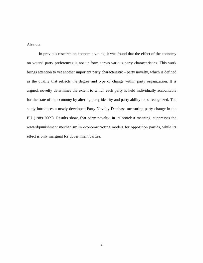
Abstract
In previous research on economic voting, it was found that the effect of the economy
on voters’ party preferences is not uniform across various party characteristics. This work
brings attention to yet another important party characteristic – party novelty, which is defined
as the quality that reflects the degree and type of change within party organization. It is
argued, novelty determines the extent to which each party is held individually accountable
for the state of the economy by altering party identity and party ability to be recognized. The
study introduces a newly developed Party Novelty Database measuring party change in the
EU (1989-2009). Results show, that party novelty, in its broadest meaning, suppresses the
reward/punishment mechanism in economic voting models for opposition parties, while its
effect is only marginal for government parties.

3
Democracy rests on accountability. Parties, being the key representative political
organizations, should be accountable to voters for their actions. Previous literature suggests
that voters tend to punish or reward parties based on a country’s economic performance. But
in order to punish a party, voters must make a mental connection between the party’s past
identity and its present identity. In other words, voters should recognize a party as essentially
the same party that existed in the previous electoral cycle. It is an intuitive task for voters if a
given party stays intact. But what if a party changes its name? Or if a party absorbs another
party and keeps its name unchanged? Or what if a new party emerged as a split from a party
in power right before elections? Would voters still punish these changed parties? More
generally, would voters still punish or reward a party even after it altered its identity?
Answering these questions would help us understand democratic accountability on a deeper
level. This paper only scratches the surface of answering these important questions and
provides a basis for future in depth research.
The array of changes parties undergo is wide. Some alter their programs, appoint new
leaders, change party names, or undergo more drastic transformations such as mergers and
splits. In addition, a small number of parties emerge as genuinely new actors. In this study,
the quality that reflects the degree of change within a party in terms of its structure (mergers,
splits, etc) and attributes (name, leader, and program) within one electoral cycle will be
called party novelty. Novelty shows how new a particular party is. At any given time any
single party has some degree of novelty. This study is set to determine how novelty shapes
and specifies the effect of economic conditions on voters’ party preferences.
In its investigation of the relationship between “party novelty” and voters’ party
preferences, this study speaks to two distinct bodies of literature. First, it contributes to our

4
understanding of voting behavior within different electoral contexts. In previous research on
economic voting, it was found that the effect of economy on party preferences is not uniform
across party level variables (Van Der Brug et al. 2007; Anderson 1995; Hibbs 1977, 1982;
Powell and Whitten 1993; Whitten and Palmer 1999). This work brings attention to yet
another important party characteristic that may condition economic voting – party novelty.
Second, this study contributes to the party development literature by highlighting
organizational (or non-policy) changes within parties and differentiating them from changes
of party policy. It distinguishes the effects of policy and non-policy changes on the electoral
success of a party.
The first section of this paper discusses the concept of party novelty, providing it with
a theoretical basis and depth. It also considers the empirical question of how common party
change is in various electoral contexts by briefly discussing the results of the comparative
study of party novelty across about 502 cases in 65 electoral contexts (covering four EU
elections – 1994, 1999, 2004, and 2009 – in 24 European countries). The second section
presents theoretical expectations and empirical tests of the relationship between the change in
voters’ party preferences and the change in party novelty across various electoral contexts.
The analysis uses two existing survey projects – European Election Study and Euromanifesto
Project – which allow comparison across 90,000 respondents in 65 electoral contexts. The
findings and directions for future research are discussed in the final section.
5
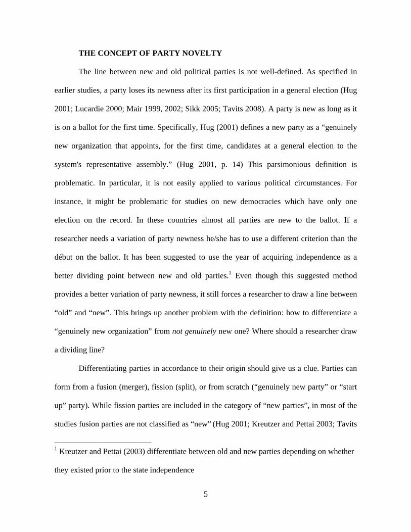
THE CONCEPT OF PARTY NOVELTY
The line between new and old political parties is not well-defined. As specified in
earlier studies, a party loses its newness after its first participation in a general election (Hug
2001; Lucardie 2000; Mair 1999, 2002; Sikk 2005; Tavits 2008). A party is new as long as it
is on a ballot for the first time. Specifically, Hug (2001) defines a new party as a “genuinely
new organization that appoints, for the first time, candidates at a general election to the
system's representative assembly.” (Hug 2001, p. 14) This parsimonious definition is
problematic. In particular, it is not easily applied to various political circumstances. For
instance, it might be problematic for studies on new democracies which have only one
election on the record. In these countries almost all parties are new to the ballot. If a
researcher needs a variation of party newness he/she has to use a different criterion than the
début on the ballot. It has been suggested to use the year of acquiring independence as a
better dividing point between new and old parties.1 Even though this suggested method
provides a better variation of party newness, it still forces a researcher to draw a line between
“old” and “new”. This brings up another problem with the definition: how to differentiate a
“genuinely new organization” from not genuinely new one? Where should a researcher draw
a dividing line?
Differentiating parties in accordance to their origin should give us a clue. Parties can
form from a fusion (merger), fission (split), or from scratch (“genuinely new party” or “start
up” party). While fission parties are included in the category of “new parties”, in most of the
studies fusion parties are not classified as “new” (Hug 2001; Kreutzer and Pettai 2003; Tavits
1 Kreutzer and Pettai (2003) differentiate between old and new parties depending on whether
they existed prior to the state independence

6
2008; Sikk 2005). Thus, in the party development literature, new parties include genuinely
new parties and fissions, and exclude electoral alliances and fusions. Parties that have simply
changed their names, programs, or leaders are not counted as new.
Even though most of the authors studying new party formation and success note the
difficulty of defining the exact border between new and established parties, many have to
draw this border for methodological reasons. Figure 1 presents this issue in schematic terms.
It shows two distributions of party cases – the one to the left represents the expectation in
common literature about the frequency of established parties and the one to the right
represents the expectation about the frequency of new ones. The longer tails of these
distributions are averted from each other showing that genuinely new parties should be very
rare, as should be truly unchanged ones. At the same time, both distributions are skewed
towards each other suggesting that most of the parties belong to the area where those two
distributions meet. This is the area where most of the literature draws the line between the
established parties and new ones. This line is very precarious as the majority of parties are
concentrated around it. Moving the line even slightly can bring a lot of new cases in or drive
quite a few cases out of the research.
Thus, where the border between established and new parties is drawn has
implications for research. For instance, the success of new parties may be either over or
underestimated depending on whether merger parties are included in a study or not.
Therefore, rather than drawing the line between new and established parties, this study views
novelty as a matter of degree. It defines party novelty as the quality that reflects the degree of
change within a party in terms of its structure and attributes within one electoral cycle2. One
2 The nature of party attributes and party structure is defined further in this section
7
of the key assumptions made in this paper is that party novelty is a quality that party acquires
within one electoral cycle. Once a party participates in general elections, its novelty is
annulled. In other words, all changes a given party underwent in the previous electoral cycle
have ‘used up’ their effect in the following election.
In order to measure party novelty, I classify parties into groups along a two
dimensional continuum. The first dimension represents the change or combination of changes
of party attributes such as party name, leader, and program. The values on this continuum are
ordered according to the ordinal scale. The ordering is theory based reflecting how a certain
party attribute should make a party more or less recognizable to ordinary voters. The change
of program is assumed to have less impact on party ability to be recognized than the change
of leader or name. Thus, the maximum on this continuum constitutes a case when a party
changed all three attributes (name, leader, and program); the minimum is when it did not
change any of them.
The second dimension represents structural changes that parties undergo. This
continuum is ordered in the similar fashion based on theoretical consideration – from no
change to the change that should alter the party identity the most in voters’ eyes. The exact
order on this dimension is as follows: (1) party stayed intact; (2) party abandoned electoral
list; (3) party joined electoral list; (4) party expanded by merger or elite defections from other
parties; (5) party suffered a split or elite defection; (6) new party emerged from the merger of
the previously existing parties; (7) new party emerged from the split of the previously
existing party; (8) new party emerged from the dissolution of the previously existing party;
(9) start up party emerged from scratch. Only parties that alter the conventional pattern of
party politics and “break the party-cartel circle” will be included in the last group (Sikk,

8
2005, p. 399). Thus, in the bottom left hand corner of the plane there would be parties that
have not changed any of their attributes and stayed structurally intact. In the upper right hand
corner of the plane there would be start up parties that have new attributes (name, leader and
program) by default.
THE EMPIRICAL DISTRIBUTION OF PARTY NOVELTY
This section explores how well the concept of party novelty describes the real world
politics. How common is the case in which a party alters its name or undergoes other
transformations? This section answers these questions by measuring party novelty in a
systematic way and presenting the results below. I constructed a database by collecting data
on change of party attributes and structure in the EU countries from one EU election to
another between 1989 and 2009. The data for this database was collected came from several
sources. All data except for the change of party program came from official party websites
and newspaper articles. Data for the change of party programs came from the Euro Manifesto
Project data for the corresponding years3.
The choice of EU countries over any other region is justified by two reasons. First of
all, EU region was chosen because it includes both – countries where we expect to see low
level of party novelty (Western Europe) as well as countries where we would expect high
level of party novelty (Eastern Europe). This expectation is primarily driven by the relative
immaturity of party systems in Eastern Europe, which manifests itself through frequent
structural and attribute-related changes within parties. Secondly, EU region provides us with
3 See Appendix B for more detailed description of data collection methodology (Appendixes
can be found here http://astro.temple.edu/~klitton/)

9
a common ground that allows systematic comparison – EU parliamentary elections. They are
conducted at the same time in all countries, which should control for general trends in the EU
politics. Also, since the EU elections are considered to be secondary to the national ones, the
presence of pre-election scandals is not likely to interfere with the results4.
The study was designed in such a way that each case represents a party per electoral
cycle – that is, a party existing between two specific elections. The same party in a different
electoral cycle is considered to be a separate unit. The nature and the combination of changes
within a specific electoral cycle give a party a certain degree of novelty. The base, to which
party changes are compared to, is the state of party structure and party attributes at the
previous general elections. Once a party participates in the next general election, its novelty
level drops to a zero and the cycle starts again. Thus, for instance, Danish social liberal party
Det Radikale Venstres (RV) between 1999 and 2004 EU elections is a separate case in the
database from the same party in 2004-2009 EU electoral cycle. In the former case, the party
has a certain degree of novelty – it suffered two splits - in May 2007 with the formation of
the New Alliance (later called Liberal Alliance) and in October 2008 with the formation of
the Borgerligt Centrum. In the later case, the party has not changes any of its attributes and it
stayed structurally intact, and therefore, had zero novelty.
The Discussion of Distribution
Some of the intuitive expectations from this comparative study are that party novelty
varies across party per electoral cycle cases and the distribution of party novelty is skewed
towards “less novelty” end. Figure 2 represents the variation of party novelty in the EU
4 See Appendix A, Table A1 for the list of countries and years (Appendixes can be found
here http://astro.temple.edu/~klitton/)

10
countries between 1989 and 2009. The axes stand for the two dimensions of party novelty
described earlier – change of party attribute (axis X) and change of party structure. Based on
the figure, there is a good variation of cases along the change of party attributes continuum
(Figure 2, X-axis). The distribution of cases is skewed towards less change as expected,
although the peaking tail on the right hints on that complete change of party attributes is not
the rarest occurrence (dashed line along the X-axis). It is important to note, however, that
about a half of the cases in the complete attribute change category (last category) are start up
parties for which the “change” of attribute was recorded by default. This accounts for the
peaking tail at the end. Furthermore, the distribution of cases along the change of party
structure continuum has even greater skewness towards less change than we see in the
distribution along the change of party attributes continuum (Figure 2, dashed line along the
Y-axis). Thus, it is apparent that parties change their attributes more readily than they change
their structure. More specifically, change of program and change of party leader are the most
common changes prates undergo. The change of name is more rare even with parties that
change their structure. The prevalence of party program and leader change, perhaps, can be
explained by the fact that parties choose transformations that would adopt them to the current
economic or political circumstances and, at the same time, that would be least costly in terms
of both votes and money. The change of name requites reprinting all of the branding
materials and it carries a greater risk for party to lose votes (or at least a greater uncertainty
about this risk).
Finally, when we combine the two dimensions of party novelty, we see that few
parties in real politics remain completely unchanged from one election to another. This is
mostly due to the fact that 78% of those parties that stayed intact changed at least one

11
attribute. The results show that there are 57 cases out of 333 (or 17.1%) in which parties
stayed structurally intact and have not changed any of its attributes (name, leader, and
program)5. This finding is crucial as it shows the importance of studying party novelty and its
effects. In more than 80 percent of cases parties changed themselves in various ways and to
various degrees, but we do not know if and how this change affected voters’ party
preferences.
PARTY NOVELTY EFFECT ON ECONOMIC VOTING
This section intends to show the effect of party novelty on democratic accountability,
specifically through the mechanism specified in the economic voting theory. The section
below will replicate the previous findings of the economic voting literature and will propose
a new conditional variable to the existing economic voting model – party novelty.
Studies on economic voting revolve around the expectation that voters’ support for
their government will be hurt by economic downfall and in some cases helped by good
economic times (Hibbs, 1977; Lewis-Beck 1988; Powell and Whitten 1993; Wlezien and
Erikson 1996; Lewis-Beck and Strgmaier (2000); Duch and Stevenson 2008). The
mechanism behind this effect comes from the view that voters’ decisions about voting, to
some extent, are policy driven. Voters evaluate current government in terms of the policy
outcomes, in this case, economy being the focal outcome (Kramer 1971, 1983; Stigler 1973;
Erikson 2004; Hibbs 2006).
5 The Party Novelty dataset includes 502 cases, but 169 cases were not included into the
graph as they have missing data on one of the party attributes . (96% of the missing cases
have missing data for the program change)
12
Most of the studies of economic voting define their dependent variable in
dichotomous fashion: as the incumbent’s vote share at the aggregate level or as a dichotomy
indicating whether the respondent voted for a government or opposition party at the
individual level6. Yet recent research has been critical of such approach (Van Der Brug, Van
Der Eijk, and Mark Franklin 2007). It is argued, that the dichotomous voting choice does not
reveal the complexity of the voting process described by Anthony Downs (1957). There are
two stages to this process. When deciding whom to vote for, before making the observable
choices (second stage), voters go through a latent (first) stage at which they form preferences
for a number of parties. It is important to emphasize that, according to this view of the voting
process, there is more than one party that voters prefer to some degree and they vote for the
party they prefer the most. This two-stage process is critical. In a situation where voters have
a clear preference for one party the slight change in party preferences due to certain factors –
such as the state of the economy – would not change the vote. But when voters’ preferences
for two parties are tied, the party choice that voters make is very delicate and volatile. In this
case, it can be influenced by the national economic conditions. Yet, if a study employs voting
as a dichotomous dependent variable, it is most likely to miss the fluctuation of voters’
preferences. Therefore, it has been suggested to use party preferences as a dependent variable
instead of the variable describing a dichotomous voting choice (Van Der Brug, Van Der Eijk,
and Mark Franklin 2007).
In this study voters’ party preferences are measured with voters’ propensity to vote
for an array of parties. It is an unusual variable as it records voters’ preferences for each
party. In order to construct this variable, this study will follow the work of Van Der Brug,
6 Aggregate incumbent vote share is used in Kramer (1971, 1983) and Paldam (1991)
13
Van Der Eijk, and Mark Franklin (2007) who use the so called “stacked data matrix.” The
“stacked data matrix” transforms the level of analysis from individual level to individual per
party level. In every survey on voting behavior respondents are treated as units of analysis
and their party preferences are set to be respondents’ attributes. The authors propose to
construct dependent variable in such a way that “each respondent appears as many times as
there are parties for which support propensities are measured.” This study adopts such
approach to measure the dependent variable and defines it as the “observed strength of
support of the respondent involved in each respondent*party combination for the party
involved in the same combination” (Van Der Brug, Van Der Eijk, and Mark Franklin 2007,
p.41‐42).
This study will not test the two-stage voting model in its entirety. It will focus on the
first stage and will attempt to predict voters’ party preferences using the economic voting
model leaving the second stage (a model that uses party preferences to predict voting choice)
to the future research project.
Independent variables and key expectations
The base model intends to replicate the most basic findings from the recent studies on
economic voting7. The model is complex as it includes variables from four levels of analysis
as well as their interactions. The levels are: individual, party, party per individual, and
national. Let me provide a basic description.
7 In particular this study will try to replicate the base model estimated by Van der Brug, Van
der Eijk, and Franklin (2007) in their volume “The Economy and the Vote” p. 88, Table 4.2,
Model F as closely as possible

14
At the individual level, the model will include a set of individual characteristics
shown to affect party support in the previous research such as age, class, religion, political
interest, education, if unemployed and if retired. In addition, some electoral studies take into
account the importance (or some use the term ‘salience’) of various political, economic and
social issues for each respondent or in aggregate (Miller, Miller, Raine and Browne 1976;
Abramowitz 1994; van der Eijk and Franklin 1996; Wlezien 2001). If a certain issue is
important to a voter, then he/she has a meaningful opinion about it, which structures his/her
support for parties. For instance, under conditions of hyperinflation, voters will evaluate
political parties based almost exclusively on parties’ ability to combat this hyperinflation.
Conversely, under stable economic conditions, non-economic issues are likely to dominate
voters’ choice. Therefore, the same macroeconomic variable may have heterogeneous effects
on voters’ choice in different countries and at different points in time. In order to control for
this possibility, issue salience should be included in the model.
Typically, the salience is measured using the “most important problem” (MIP) survey
question. There have been concerns that this is a limited (not complete, asymmetrical)
measure of issue importance, given it doesn’t take into consideration importance of issues
that are not “problems” per se (Wlezien 2005). But in the absence of an alternative
instrument, this study will use the MIP survey question to control for the effect of issues on
voters’ party evaluations8. It also works fairly well (see Soroka and Wlezien, 2010).
8 The variable is constructed in a following way. The MIP question is used to construct a
series of dummy variables. Each of the dummies indicates if a particular respondent
considers a certain issue to be the most important problem. For instance, there is a dummy
variable indicating if respondents think of labor market conditions to be the most important

15
At the party level, the study will test if government parties experience “cost of
governing” losses seen in previous studies (Powell and Whitten 1993; Paldam 1991;
Nannestad and Paldam 1994, 2002). According to these studies, the estimated loss of
incumbent party popularity is at about 2.5 percent. Government parties are expected to lose
support simply as a result of incumbency. It order to test this effect the model includes a
party level dummy variable measuring whether a given party was a governing party or was in
a governing coalition for the past electoral cycle.
Secondly, the model includes a party size variable with the expectation that the larger
the party the more the voters hold it accountable for the economic performance (Van der
Brug, Van der Eijk, and Franklin 2007). Party size is measured by the proportion of seats in
the national parliament.
At the individual per party level, the model will attempt to mimic aggregate level
economic voting studies which control their models for the previous vote share of governing
parties9. In order to do that it will include an individual level dummy variable indicating
problem in the country. Other dummies include, but not limited to: government, inflation,
welfare, economy of a nation in general, health and food safety, foreign policy, environment
and energy, corruption and crime, infrastructure, immigration and minorities, and other social
and economic issues. These dummies are used to calculate predicted values (y-hat) of voters’
propensities to vote for particular parties. Thus, the base model itself uses this y-hat variable
as a control for the effect of issue salience on voters’ party preferences.
9 Same variable was included in the economic voting models estimated by Van der Brug,
Van der Eijk, and Franklin (2007)

16
whether a certain respondent voted for the particular party in the previous elections10. This
variable is also suited for controlling for partisanship and other individual level variables not
included in the model. It is expected to have a positive effect on party support – if a
respondent voted for the particular party in last elections, he is likely to do the same in the
current election.
In addition, it is necessary to control for the spatial effect on the left-right scale – that
is, the difference between respondents’ positions and their perception of parties’ positions on
the left right scale. Respondents should prefer parties closest to their own issue positions. The
smaller the distance between the respondent’s position and the party position the greater
respondent’s utility and, thus, the more likely this respondent to prefer this particular party
(Downs 1957). Thus, the effect of distance is expected to be negative. Taking into account
the fact that the unit of analysis is respondent per party, it should be easy to include a
variable measuring the distance between respondent’s position and the perceived position of
each party on the left right scale 11.
Finally, previous studies found that the effect of the left-right proximity on party
preference varies across political systems. This variance can be accounted for by calculating
the extent of the perceptual agreement (Oppenhuis 1995). It measures the degree to which
10 It is important to remember here, that the units of analysis are “party per respondent”.
11 The variable is constructed by calculating Euclidean distances between respondent’s
position and his/her perceived position of each party on the left-right scale
17
respondents in each country agree on the position of the political parties on the left-right
scale12.
At the national level, the model will test the effect of the economic and institutional
conditions. In some studies, the effect of the economic conditions is detected through
correlating voters’ economic perceptions with their voting choice (Fiorina 1981; Lewis-Beck
1988; Alvarez and Nagler 1995, 1998). However, using voters’ perceptions of economic
conditions may be problematic. The causation flow from voters’ economic perceptions to
their voting choice has been accused of endogeneity (Wlezien, Franklin, and Twiggs 1997;
Lewis-Beck and Stegmaier 2000). Party identification is believed to be the source of this
problem (Andersen et al 2004; Evans 1999; Evans and Andersen 2006; Johnston et al 2005; Wilcox and
Wlezien 1996; Wlezien, Franklin, and Twiggs 1997). Voters’ ideological disposition affects voters’
perceptions through a “perceptual screen” – a concept introduced by Campbel et al (1960)
and applied to economic voting by Conover et all (1987). In order to mitigate endogeneity
some suggest controlling for partisan identification (Evans and Andersen, 2006)13.
The concerns that the effect of the economic perceptions is overestimated due to
endogeneity have been mounting until very recent study by Lewis-Beck, Nadeau, and Elias
(2008). The authors argue that while the bias caused by endogeneity indeed exists it is
12 This measure was calculated using the procedure described in Van der Eijk (2001) and
STATA algorithm ("agrm") developed by Alejandro Ecker
13A number of studies put out more far reaching critique arguing that economic expectations
are not exogenous to politics as it was previously assumed.13 In their recent study Ladner and
Wlezien (2007) showed that voters’ economic expectations are affected not only by voters’
support for incumbents but also by their forecasts of the electoral outcome

18
substantially downward. In order to eliminate endogeneity, the authors utilized panel data
instead of commonly used cross-sectional data. They concluded that in panel data research
design the effect of the economic perceptions is even greater than the effect reported in cross-
sectional studies. Others are less sanguine about the use of the economic perceptions in the
model of economic voting (Evans and Pickup 2010). There is no guarantee that the issue is
put at rest as the authors do not question the existence of endogeneity in the cross-sectional
economic voting models. In order to avoid dealing with endogeneity, this study uses
objective measurement of the economy – the level of economic growth, inflation, and
unemployment. The number of economic contexts (in total 67) permits the use of the
objective measures without under-specifying the model of economic voting.
Thus, to test the key hypothesis fundamental to the economic voting literature, the
model includes national level economic indicators and their interactions with the party
incumbency dummy. The expectation is that economic growth has a positive effect on voters’
support for government party, while inflation and unemployment have negative effects. It
addition it is expected that the effects of the economy on voters’ support for opposition
parties will be smaller or differently-signed than for government parties.
Among other notable determinants of party support are system characteristics.
Specifically, the clarity of responsibility within a political system is believed to mediate the
effects of the economy (Powell and Whitten 1993; Whitten and Palmer 1999; Van Der Brug,
Van Der Eijk, and Mark Franklin 2007). Given the comparative nature of this study, it is
essential to take into account institutional differences between political contexts. Powell and
Whitten’s (1993, p. 398-406) construct the clarity of responsibility index from five measures
recording whether there was: a weak party cohesion, a chairmanship of legislative
19
committees by opposition parties, a bicameral opposition, a minority government, a coalition
government.
For the past two decades the index has been refined, so some recent studies use
slightly altered clarity of responsibility index. In order to calculate the index and classify the
countries, this work uses methodology developed by Tavits (2007, p.221) who relies on
Powell’s (2000) work. Thus, the index used in this study has four composites: government
majority status, cabinet duration, opposition influence, and the effective number of parties14.
The key hypotheses of this study specify expectations of whether and how party
novelty affects voters’ party preferences in different economic circumstances. It is argued
that the main mechanism lies through the alteration of party identity. It is assumed Certain
party transformations are more significant than others and they presumably are more
recognizable to voters. Party identity is understood in terms of a visible party presence, the
one that is apparent to common voters with little to no interest in politics. Thus, in this study,
those structural or attribute changes within parties that can be seen by voters without them
having to obtain in depth knowledge are expected to alter party identity the most and, in turn,
are expected to have greater effect on voters’ party preferences15.
14 The index has to be calculated anew as: (1) this study includes recent governments (up to
2009), which were not included in the calculations by Powell’s (2000) or Tavits (2007); (2)
some of the composite elements of the index are time sensitive – that is, for every country
each additional government alters the score. See Appendix B for details on how it was
constructed
15 The sources of such in depth knowledge could be party statutes, extensive news
reports, or party program.

20
In sum, this study will test the following hypotheses:
H1: Party novelty has the conditional effect on voters’ propensity to vote for parties
given various economic circumstances.
H2: Both dimensions of party novelty (structural and attribute change) as well as their
internal elements are expected to have a conditional effect on voters’ propensity to vote for
parties given various economic circumstances.
H3: The effect specified in H2 should be seen in both government and opposition
parties.
H4: In improving economic circumstances, government parties should loose from
greater degrees of party novelty (or its dimensions or their internal elements), while when
economy goes down government parties should benefit from greater degrees of party
novelty.
H5: In improving economic circumstances opposition parties should benefit from
greater degrees of party novelty (or its dimensions or their internal elements). However in
deteriorating economic circumstances opposition parties should not either benefit or loose
from greater degrees of party novelty.
H7: Those elements of party novelty that alter party identity the most are expected to
have stronger effect than those than do not. For instance, within change of party attribute
dimension, change of party program is expected to have weaker conditional effect on this
party popularity than change of party name. Likewise, within change of party structure
dimension, leaving electoral alliance should have weaker conditional effect on this party
popularity than suffering a split or even weaker than starting party from scratch.
Data and Methods
21
The data measuring voters’ party preferences can be found in two large cross-national
studies: Comparative Study of Electoral Systems (CSES) and the European Election Studies
(EES). In the CSES, voters’ party preferences are measured using the feeling thermometer,
while in EES it is measured with voters’ propensity to support particular parties (PTV).
There is a reason to believe that PTV is a better measurement of voters’ party
preferences. Some advocate the use of the propensity measure as it was found to have the
stronger relation with voting choice than feeling thermometers (Van Der Brug, Van Der Eijk,
and Mark Franklin 2007). For instance it was established that whereas in 93 percent of the
cases the party choice matches the party with the highest score on the support propensity
measure, the match rate for feeling thermometer was much lower at 73 percent (Kroh 2003).
Since this study is interested in voters’ party preferences provided that ultimately they affect
voting choice, PTVs appear to be a better measure of voters’ party preferences. Therefore,
the data for the dependent variable as well as for some individual, party and country level
variables will come from the European Election Study (EES). It has been conducted during 7
consecutive elections for European Parliament between 1979 and 2009.
Another reason for the use of the EES is spelled out by Van Der Brug, Van Der Eijk,
and Mark Franklin (2007) – they encourage the use of the EES as elections to European
Parliament are “uncontaminated by the idiosyncrasies of national elections”. In other words,
EU elections are relatively free from the effect of the campaign slogans, candidates’
appearance, political scandals and other nonrandom noise that is commonly associated with
national elections.
Also, a few words should be said on cyclicality in EU elections. Since the data is
collected for the EU parliamentary elections, which in most of the cases do not coincide with
22
national parliamentary elections, the model should control for the effect of the electoral cycle
on popularity of incumbent parties. It has been observed that government party popularity
drops in the middle of the cycle. The popularity seems to go down in the first half of the
cycle regardless of government performance: that is either due to government inability to
satisfy conflicting demands from various groups of voters (Downs, 1957) or because the
opposite is true – government satisfying demands for policies that brought them into office in
the first place (Wlezien 1995, 2004; Franklin and Wlezien 1997; Bafumi, Erikson, and
Wlezien 2010). According to the latter view, in the second half of the cycle the popularity of
incumbent parties tends to go up as they start framing new issues and formulating new
policies in anticipation of the upcoming election16.
Furthermore, there are a few ways to measure the economic conditions in a country
for a certain electoral cycle. The change measures make more sense for comparative research
than the static measures. While the latter simply captures the state of the economy at a given
point in time, the former highlight the trend – whether the economy got better or worth – that
is more likely to be registered by voters. Therefore, the following indicators were used for
the economic voting models: a percentage change in real GDP for a year of the election as
compared to the previous year (i.e. real GDP growth), a percentage in annual rate of
unemployment for a year of the election as compared to the previous year, a percentage
change in prices for a year of the election as compared to the previous year (i.e. annual
inflation rate). Data measuring economic growth, inflation, and unemployment is obtained
from the OECD online database.
16 See Appendix B for how the variable was constructed
23
Finally, to estimate the model I use OLS with country and year dummies and with
robust errors calculated at the individual level, not individual per party level. The errors are
calculated at the individual level in order to deal with the fact that respondents give different
patterns of answers to the PTV questions (remember that the data is stacked, so the same
respondent is appearing several times in the data)17. For instance stronger identifiers will
single out one party with a high PTV score; weaker identifiers will give same PTV scores to
two or more parties.
Results
As stated above, the analysis starts with replication of the economic model in which
all government parties are held equally accountable for the state of the economy no matter
what degree of novelty they have. After running models with various combinations of
economic indicators it became apparent that models using GDP growth and unemployment
rate generate statistically significant interactions with signs that confirm theoretical
expectations. Models that use inflation and misery index as economic measures do not yield
robust results.18 Since GDP measure is more consistent across countries than the measure of
unemployment, the model using GDP growth is more reliable. Therefore, models, discussed
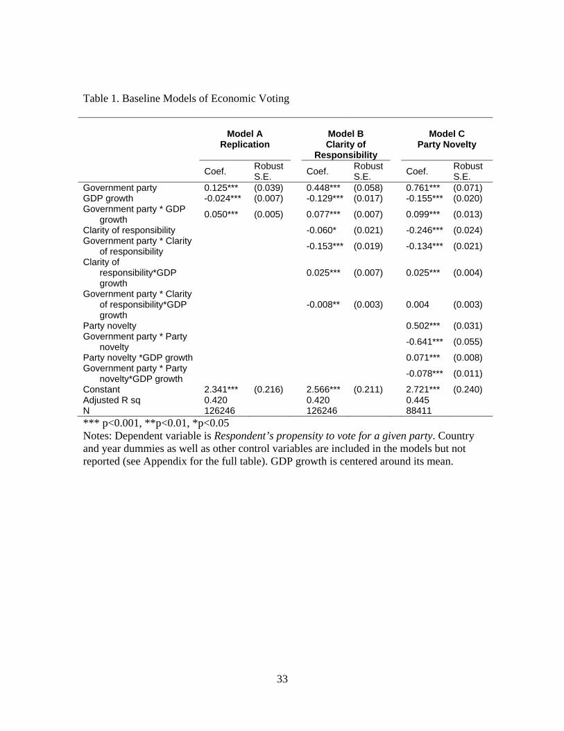
further in the paper, are built based on the GDP growth model (see Table 1. Model A).
From the Model A estimates, the joint effect of the GDP growth and party
government status has a positive sign which supports the findings of the previous literature
17 See similar procedure in Van Der Brug, Van Der Eijk, and Mark Franklin (2007)
18 The Base models testing the effect of unemployment, inflation, and misery index are not
shown. See Appendix A, Table A2
24
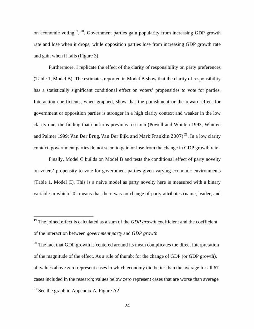
on economic voting19, 20. Government parties gain popularity from increasing GDP growth
rate and lose when it drops, while opposition parties lose from increasing GDP growth rate
and gain when if falls (Figure 3).
Furthermore, I replicate the effect of the clarity of responsibility on party preferences
(Table 1, Model B). The estimates reported in Model B show that the clarity of responsibility
has a statistically significant conditional effect on voters’ propensities to vote for parties.
Interaction coefficients, when graphed, show that the punishment or the reward effect for
government or opposition parties is stronger in a high clarity context and weaker in the low
clarity one, the finding that confirms previous research (Powell and Whitten 1993; Whitten
and Palmer 1999; Van Der Brug, Van Der Eijk, and Mark Franklin 2007) 21. In a low clarity
context, government parties do not seem to gain or lose from the change in GDP growth rate.
Finally, Model C builds on Model B and tests the conditional effect of party novelty
on voters’ propensity to vote for government parties given varying economic environments
(Table 1, Model C). This is a naive model as party novelty here is measured with a binary
variable in which “0” means that there was no change of party attributes (name, leader, and
19 The joined effect is calculated as a sum of the GDP growth coefficient and the coefficient
of the interaction between government party and GDP growth
20 The fact that GDP growth is centered around its mean complicates the direct interpretation
of the magnitude of the effect. As a rule of thumb: for the change of GDP (or GDP growth),
all values above zero represent cases in which economy did better than the average for all 67
cases included in the research; values below zero represent cases that are worse than average
21 See the graph in Appendix A, Figure A2
25
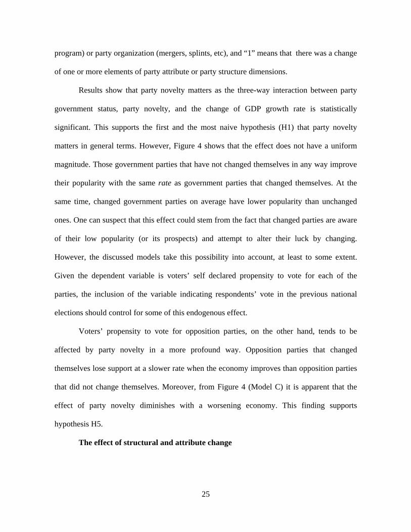
program) or party organization (mergers, splints, etc), and “1” means that there was a change
of one or more elements of party attribute or party structure dimensions.
Results show that party novelty matters as the three-way interaction between party
government status, party novelty, and the change of GDP growth rate is statistically
significant. This supports the first and the most naive hypothesis (H1) that party novelty
matters in general terms. However, Figure 4 shows that the effect does not have a uniform
magnitude. Those government parties that have not changed themselves in any way improve
their popularity with the same rate as government parties that changed themselves. At the
same time, changed government parties on average have lower popularity than unchanged
ones. One can suspect that this effect could stem from the fact that changed parties are aware
of their low popularity (or its prospects) and attempt to alter their luck by changing.
However, the discussed models take this possibility into account, at least to some extent.
Given the dependent variable is voters’ self declared propensity to vote for each of the
parties, the inclusion of the variable indicating respondents’ vote in the previous national
elections should control for some of this endogenous effect.
Voters’ propensity to vote for opposition parties, on the other hand, tends to be
affected by party novelty in a more profound way. Opposition parties that changed
themselves lose support at a slower rate when the economy improves than opposition parties
that did not change themselves. Moreover, from Figure 4 (Model C) it is apparent that the
effect of party novelty diminishes with a worsening economy. This finding supports
hypothesis H5.
The effect of structural and attribute change
26
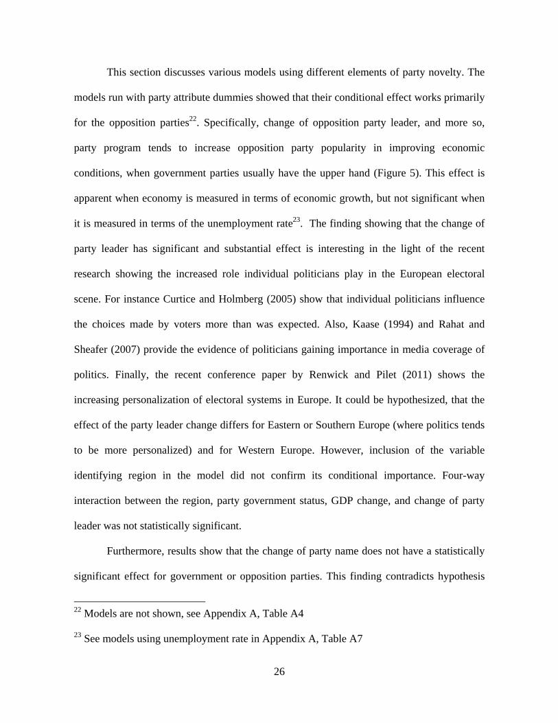
This section discusses various models using different elements of party novelty. The
models run with party attribute dummies showed that their conditional effect works primarily
for the opposition parties22. Specifically, change of opposition party leader, and more so,
party program tends to increase opposition party popularity in improving economic
conditions, when government parties usually have the upper hand (Figure 5). This effect is
apparent when economy is measured in terms of economic growth, but not significant when
it is measured in terms of the unemployment rate23. The finding showing that the change of
party leader has significant and substantial effect is interesting in the light of the recent
research showing the increased role individual politicians play in the European electoral
scene. For instance Curtice and Holmberg (2005) show that individual politicians influence
the choices made by voters more than was expected. Also, Kaase (1994) and Rahat and
Sheafer (2007) provide the evidence of politicians gaining importance in media coverage of
politics. Finally, the recent conference paper by Renwick and Pilet (2011) shows the
increasing personalization of electoral systems in Europe. It could be hypothesized, that the
effect of the party leader change differs for Eastern or Southern Europe (where politics tends
to be more personalized) and for Western Europe. However, inclusion of the variable
identifying region in the model did not confirm its conditional importance. Four-way
interaction between the region, party government status, GDP change, and change of party
leader was not statistically significant.
Furthermore, results show that the change of party name does not have a statistically
significant effect for government or opposition parties. This finding contradicts hypothesis
22 Models are not shown, see Appendix A, Table A4
23 See models using unemployment rate in Appendix A, Table A7
27
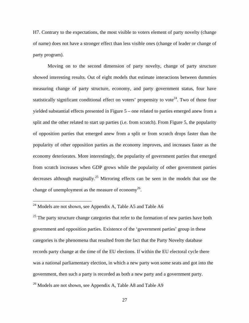
H7. Contrary to the expectations, the most visible to voters element of party novelty (change
of name) does not have a stronger effect than less visible ones (change of leader or change of
party program).
Moving on to the second dimension of party novelty, change of party structure
showed interesting results. Out of eight models that estimate interactions between dummies
measuring change of party structure, economy, and party government status, four have
statistically significant conditional effect on voters’ propensity to vote24. Two of those four
yielded substantial effects presented in Figure 5 – one related to parties emerged anew from a
split and the other related to start up parties (i.e. from scratch). From Figure 5, the popularity
of opposition parties that emerged anew from a split or from scratch drops faster than the
popularity of other opposition parties as the economy improves, and increases faster as the
economy deteriorates. More interestingly, the popularity of government parties that emerged
from scratch increases when GDP grows while the popularity of other government parties
decreases although marginally.25 Mirroring effects can be seen in the models that use the
change of unemployment as the measure of economy26.
24 Models are not shown, see Appendix A, Table A5 and Table A6
25 The party structure change categories that refer to the formation of new parties have both
government and opposition parties. Existence of the ‘government parties’ group in these
categories is the phenomena that resulted from the fact that the Party Novelty database
records party change at the time of the EU elections. If within the EU electoral cycle there
was a national parliamentary election, in which a new party won some seats and got into the
government, then such a party is recorded as both a new party and a government party.
26 Models are not shown, see Appendix A, Table A8 and Table A9
28
It is worth noting that the above findings support theoretical assumptions made in the
previous studies in which a merger is not considered to be an identity-altering transformation
of a party, while a split is considered to have an identity-altering effect (Hug 2001; Kreutzer
and Pettai 2003; Tavits 2008; Sikk 2005). This paper views alteration of party identity as an
essential part of the mechanism through which structural and attribute change within a party
affects its popularity. Therefore, the fact that the emergence of a party anew from a split has
a significant effect on party popularity while the emergence of a party anew from a merger
does not, given certain economic conditions, tells us that the former alters party identity more
than the latter (although findings are true only for opposition parties).
Dummy variables measuring less severe structural change – such as abandonment or
entrance into an electoral coalition – did not show statistically significant results. The dummy
representing parties that emerged anew from dissolution also proved to be insignificant for
either GDP growth or unemployment rate measures of economic conditions.
All in all, in contrast to the attribute dimension, the structural dimension of the party
novelty concept shows a pattern expected in hypothesis H7. Those dummy variables that
measure less severe structural change (abandonment or entrance into electoral coalition) have
insignificant or weak effect on voters’ propensities to vote than those that measure more
severe structural change (new splinter and start up parties).
Finally, the results did not support the expectations made in hypothesis H3 stating
that the effect of party novelty or its elements should be seen in both government and
opposition parties. Clearly, the results are more significant and substantial for opposition
parties than for government ones. As a result, hypothesis H4 stating expectations for
government parties did not hold as well.

29
CONCLUSION
This study explored the concept of party novelty and its effects on voter’s party
preferences. In the first half, the paper defined party novelty as the quality that reflects the
degree of change within a party in terms of its structure and attributes within one electoral
cycle and highlighted its empirical relevance. To sum up, it established that in more than 80
percent of cases parties changed themselves in various ways and to various degrees.
Consequently, it raised a question of whether and how this variation affects voters’ party
preferences. This question was explored in the second half of the paper.
The finding that surfaces the most is that it is beneficial for opposition parties to
change their attributes in improving economic conditions when government parties usually
have the upper hand. By changing, they avoid loosing as much support as they would if they
did not change. However, opposition parties should avoid severe structural transformations
such as creating new splinter parties or starting parties anew from scratch when the economy
improves.
The consequences of these findings are quite interesting. First of all, they tell us that
change of and within party organization matters for estimating party support among voters.
Party policy stance is not the only party characteristic voters base their preferences on.
Furthermore, up to now, economic voting models used only party incumbency, ideology, and
30
party size to account for party level effects on voters’ party support. The significant and
substantial effect of certain elements of party novelty draws attention to party change as an
important predictor in the economic voting models.
By highlighting party novelty as an important predictor of voters’ party preferences,
this study attempted to bring two fields of political research together – the one that is focused
on party development and another that is focused on political behavior. Yet, there are a lot of
questions that are still left open for both bodies of literature. On the one hand, it is imperative
to study what explains party novelty, and party development literature offers a number of
possible explanations to test in this regard. Also, future research should explore the
possibility of more efficient operationalization of party novelty as a categorical variable
rather than as a series of dichotomous ones.
On the other hand, literature on political behavior opens up possibilities for future
research as well. For instance, it is interesting to know if the timing of change matters. In
other words, will a party do better or worse if it changes immediately before the elections
given various economic conditions? Furthermore, this paper makes an assumption that voters
are not sophisticated – that is, they base their judgment only on the most visible changes and
do not have in-depth knowledge of the political developments. Future research should relax
this assumption and see if the effect of party novelty and its elements is the same for
knowledgeable and ignorant voters. And, finally, it would be valuable to examine the effect
of party novelty on other aspects of accountability besides the economy, such as, policy
representation. In the meantime, we know that what parties do can matter to what voters do
on Election Day.

31
TABLES AND FIGURES
Figure 1. Presumed Party Novelty Distribution
s
Genuinely new party
The presumed distribution of all kinds of ‘established’ parties as defined in the party development literature
Fully established (truly unchanged) party
The line is drawn somewhere here depending on the author
The presumed distribution of all kinds of ‘new’ parties as defined in the party development literature

32
Figure 2. Distribution of Cases on the Change of Party Attributes and Change of
Party Structure Continuum27
Intact
Abandoned electoral list
Joined electoral list
Expanded by merger ordefections from other
Suffered a split
New from merger
New from split
New from dissolution
Start up
No change
Program only
Leader only
Leader andProgram
Name only
Name and Program
Name and Leader
Name, Leader, and
Program
Attribute change (the change of...)
Str
uc
tura
l ch
an
ge
17.1%(57 cases)
4.2%(14 cases)
0.3%(1 case)
24.6%(82 cases)
27 Only the cases that have no missing data were included. In total 333 cases.
Overwhelming majority of cases were excluded because of the missing data on party
program change
33
Table 1. Baseline Models of Economic Voting
Model A
Replication Model B
Clarity of Responsibility
Model C Party Novelty
Coef. RobustS.E.
Coef.
RobustS.E.
Coef.
RobustS.E.
Government party 0.125*** (0.039) 0.448*** (0.058) 0.761*** (0.071) GDP growth -0.024*** (0.007) -0.129*** (0.017) -0.155*** (0.020) Government party * GDP
growth 0.050*** (0.005) 0.077*** (0.007) 0.099*** (0.013)
Clarity of responsibility -0.060* (0.021) -0.246*** (0.024) Government party * Clarity
of responsibility -0.153*** (0.019) -0.134*** (0.021)
Clarity of responsibility*GDP growth
0.025*** (0.007) 0.025*** (0.004)
Government party * Clarity of responsibility*GDP growth
-0.008** (0.003) 0.004 (0.003)
Party novelty 0.502*** (0.031) Government party * Party
novelty -0.641*** (0.055)
Party novelty *GDP growth 0.071*** (0.008) Government party * Party
novelty*GDP growth -0.078*** (0.011)
Constant 2.341*** (0.216) 2.566*** (0.211) 2.721*** (0.240) Adjusted R sq 0.420 0.420 0.445 N 126246 126246 88411 *** p<0.001, **p<0.01, *p<0.05 Notes: Dependent variable is Respondent’s propensity to vote for a given party. Country and year dummies as well as other control variables are included in the models but not reported (see Appendix for the full table). GDP growth is centered around its mean.

34
Figure 3. Interaction between party incumbency and Economic growth (Model A)
3.1
3.2
3.3
3.4
3.5
3.6
3.7
3.8
3.9
-5 -3 -2 -1 0 1 2 3 5
Change in GDP (from previous year)
PT
V
Opposition Parties
Government Parties

35
Figure 4. The conditional effect of party novelty on voters’ propensities to vote for particular parties (Model C)
-0.2000
0.0000
0.2000
0.4000
0.6000
0.8000
1.0000
1.2000
1.4000
-5 -3 -2 -1 0 1 2 3 5
GDP growth
PT
V
Opposition party, no novelty
Government party, no novelty
Opposition party, yes novelty
Government party, yes novelty

36
Figure 5. The effect of structural and attribute change on voters’ propensities to vote for
parties
Selected categories of Attribute change
Change of leader Change of program
0
0.5
1
1.5
2
2.5
3
3.5
4
4.5
-5 -3 -2 -1 0 1 2 3 5
Change in GDP
PT
V
Opposition party that did not change its leader
Government party that did not change its leader
Government party that changed its leader
Opposition party that changed its leader 3.2
3.4
3.6
3.8
4
4.2
4.4
-5 -3 -2 -1 0 1 2 3 5
Change in GDP
PT
V
Opposition party that did not change its program
Government party that did not change its program
Government party that changed its program
Opposition party that changed its program
Selected categories of Structural change
Emerging anew from a split Emerging anew from scratch
0
0.5
1
1.5
2
2.5
3
3.5
4
4.5
-5 -3 -2 -1 0 1 2 3 5
Change in GDP
PT
V
Opposition party that did not emerge as new from a split
Government party that did not emerge as new from a split
Government party that emerged as new from a split
Opposition party that emerged as new from a split
0
0.5
1
1.5
2
2.5
3
3.5
4
4.5
-5 -3 -2 -1 0 1 2 3 5
Change in GDP
PT
V
Opposition non start up party
Government non start up party
Government start up party
Opposition start up party

37
BIBLIOGRAPHY
Curtice, John, and Sören Holmberg. 2005. “Party Leaders and Party Choice.” In The
European Voter. A Comparative Study of Modern Democracies, ed. Jacques
Thomassen. Oxford: Oxford University Press, 235-53.
Downs, Anthony. 1957. An Economic Theory of Democracy. New York: Harper and Row
Evans, Geoffrey, and Robert Andersen. 2006. “The Political Conditioning of Economic
Perceptions.” Journal of Politics 68(1): 194–207.
Fiorina. 1981. Retrospective Voting in American Elections. New Haven: Yale University
Press.
Gallagher, Michael, and Paul Mitchell. 2008. “Appendix B.” In The Politics of Electoral
Systems, eds. Michael Gallagher and Paul Mitchell. Oxford and New York:
Oxford University Press.
Hug, Simon. 2001. Altering Party Systems: Strategic Behavior and the Emergence of
New Political Parties in Western Europe. Ann Arbor: University of Michigan
Press.
Kaase, Max. 1994. “Is there a personalization in politics? Candidates and Voting
Behavior in Germany.” International Political Science Review 15(3): 211-30.
Kramer, Gerald. 1971. "Short-Term Fluctuations in U.S. Voting Behaviour, 1896-1964."
American Political Science Review 65(1):131-43.
Lane, Robert, 1962, Political Ideology. New York: Free Press.
Lewis-Beck, Michael. 1988. Economics and Elections: the major Western Democracies.
Ann Arbour: University of Michigan Press.
38
Lucardie Paul. 2000. Prophets, Purifiers and Prolocutors: Towards a Theory on the
Emergence of New Parties, Party Politics 6(2): 175-185.
Mair, Peter. 2002. “In the Aggregate: Mass Electoral Behavior in Western Europe.” In
Comparative Democratic Politics, ed. Hans Keman. London: Sage, 122–140.
Miller, Arthur H., and Thomas F. Klobucar. 2000. “The Development of Party
Identification in Post-Soviet Societies.” American Journal of Political Science,
44(4): 667-686.
Paldam, Martin. 1991. “How Robust is the Vote Function? A Study of 17 Countries Over
Four Decades,” In Economics and Politics: The Calculus of Support, eds. Helmut
Norpoth, Michael Lewis-Beck, and Jean-Dominique Lafay. Ann Arbor:
University of Michigan Press, 9-31.
Powell, G. Bingham, and Guy Whitten. 1993. "A Cross-National Analysis of Economic
Voting: Taking Account of Political Context." American Journal of Political
Science 37(2): 391-414.
Rahat, Gideon and Tamir Sheafer. 2007. “The personalization(s) of politics: Israel 1949-
2003.” Political Communication 24(1): 65-80.
Renwick, Alan, and Jean-Benoit Pilet. 2011. The Personalization of Electoral Systems:
Theory and European Evidence. Presented at the ECPR General Conference,
Reykjavik.
Sikk, Allan. 2005. "How unstable? Volatility and the Genuinely New Parties in Eastern
Europe" European Journal of Political Research 44(3): 391-412
Tavits Margit. 2007. “Clarity of Responsibility and Corruption.” American Journal of
Political Science 51(1): 218-229

39
Tavits, Margit, 2006 “Party System Change: Testing a Model of New Party Entry.” Party
Politics, 12(1): 99–119.
Tavits, Margit. 2008. "Party Systems in the Making: The Emergence and Success of New
Parties in New Democracies." British Journal of Political Science, 38 (1): 113-
133.
Van Der Brug, Wouter, Cees Van Der Eijk, and Mark Franklin. 2007. The Economy and
the Vote: Economic Conditions and Elections in Fifteen Countries. Cambridge
University Press.
Wlezien, Christopher, and Robert S. Erikson. 1996. Temporal Horizons and Presidential
Election Forecasts. American Politics Research 24(4): 492-505.
Wlezien, Christopher, Mark Franklin, and Daniel Twiggs. 1997. “Economic Perceptions
and Vote Choice: Disentangling the Endogeneity.” Political Behavior 19(1): 7-17.
Wlezien, Christopher. 2005 . “On the Salience of Political Issues: The Problem with
‘Most Important Problem’.” Electoral Studies 24(4): 555-79.
Zaller, John. 2004. “Floating Voters in U.S. Presidential Election, 1948-2000.” In Studies
in Public Opinion: Attitudes, Nonattitudes, Measurement Error, and Change, eds.
Willem E. Saris, and Paul M. Sniderman. Princeton, NJ: Princeton University
Press, 166-214.
Ladner, Matthew, and Christopher Wlezien. 2007. “Partisan Preferences, Electoral
Prospects, and Economic Expectations.” Comparative Political Studies 40(5):
571-596.
Wlezien, Christopher. 2001. "On Forecasting the Presidential Election Vote," PS:
Political Science and Politics, XXXIV (1): 25-32.

40
Wilcox, Nathaniel, and Christopher Wlezien. 1996. The contamination of responses to
survey items: Economic perceptions and political judgments. Political Analysis
5(1): 181-213.
Evans, Geoffrey and Mark Pickup. 2010. “Reversing the Causal Arrow: The Political
Conditioning of Economic Perceptions in the 2000–2004 U.S. Presidential
Election Cycle.” The Journal of Politics 72: 1236-1251.
Bafumi, Joseph, Robert S. Erikson and Christopher Wlezien. 2010. “Ideological Balancing,
Generic Polls and Midterm Congressional Elections.” Journal of Politics 72: 705-
719.