Embed Size (px)
Citation preview
Particle Formation, Growth and Transport on the Molecular and Submicron
Scale
A DISSERTATION
SUBMITTED TO THE FACULTY OF
UNIVERSITY OF MINNESOTA
BY
Chenxi Li
IN PARTIAL FULFILLMENT OF THE REQUIREMENTS
FOR THE DEGREE OF
DOCTOR OF PHILOSOPHY
Professor Christopher J Hogan Jr.
Professor Peter H McMurry
November 2018

© Chenxi Li 2018
i
Acknowledgements
This thesis is the fruit of four years of graduate study at the University of
Minnesota. I am deeply grateful to people who have contributed to this work, directly or
indirectly. Though all of you cannot be recognized by name here, I thank all of you from
my heart.
First, special recognition is due both my advisors, Dr. Chris Hogan and Dr. Peter
McMurry. I am sincerely grateful that I am co-advised by two highly intelligent and
caring professors who offered me guidance and gentle supervision. Their intellectual
support and vision enabled me to gain confidence and mature as a researcher; their
passion for work motivated me to pursue my scientific and creative interests; their
feedback was most essential to the completion of all the work presented in this thesis.
Without their support, this dissertation would not have been possible.
I have been fortunate to have worked with many other researchers during the
course of my graduate study. In particular, I would like to thank Dr. Thomas
Schwartzentruber, Narendra Singh, Dr. Bernard Olson and Dr. Dylan Millet. Their
expertise on aerodynamic drag, impaction and mass spectrometry are reflected in the last
two studies of this thesis. Additionally, I would like to thank Dr. Kenjiro Iida and Lauri
Ahonen for our collaboration on tandem particle mobility-mass measurements.
I shall always cherish the rapport among my laboratory members and the
mechanical engineering department. I thank my co-workers and friends Mark
Stolzenburg, Siqin He, Seongho Jeon, Jikku Thomas, David Buckley, Xiaoshuang Chen,

ii
Huan Yang, Souvik Gosh, Jihyeon Lee and Yuechen Qiao for the knowledge we shared
and the good times we had together.
Finally, I owe special thanks to my parents, Jimei Sun and Jianfang Li, and my
girlfriend, Yue Yu. My parents’ faith in me is the foundation for everything that I have
accomplished. Yue’s encouragement helped me survive the most difficult times; her
emotional and intellectual support has been the most valuable thing to me throughout the
past four years.
iii
Abstract
Nanoparticle formation, growth and transport are important topics in several
contexts, such as cloud formation, particle synthesis and additive manufacturing. This
thesis approaches the subject with a broad perspective from molecular to the micro- scale,
utilizing theoretical analysis, computational simulation as well as experiment
observations.
First, general dynamic equations are non-dimensionalized and applied to simulate
aerosol formation and growth in a constant rate reaction reactor. Dimensionless equations
lead to results that are independent of condensing species formation rates. The effect of
particle sink processes (e.g. evaporation, wall loss, loss to preexisting particles and
dilution) and acid-base reactions are systematically investigated. Errors involved with
common methods used for deducing particle growth rates from experimental observations
are discussed. The results suggest the maximum overestimation error for true particle
growth rates occurs when particle nucleation and growth are collision controlled.
Second, tandem mobility-mass spectrometry is utilized to understand sorption of
organic vapors onto cluster ions. It is found that cluster structure, polarity and the
molecular structure of the condensing vapors all influence uptake by cluster ions,
qualitatively in agreement with previous activation efficiency measurements for
condensational particle counters.
Third, nanoparticle transport in an aerosol deposition device is probed with fluid
dynamics and particle trajectory simulations. To facilitate particle trajectory simulations,
a neural network based drag law is developed that can be applied over a wide range of

iv
Knudsen and Mach numbers. Simulation results reveal both particle impaction speeds
and particle focusing effects are size dependent, with optimal particle sizes for
maximizing particle impaction speed and focusing. With a newly developed framework,
mass, momentum and kinetic energy fluxes from particles to the substrate are calculated.
It is shown the kinetic energy flux can be above 104 W m-2 for modest aerosol
concentrations due to particle focusing.
Finally, classification and prediction of different types of lung cell are performed
with machine learning algorithms, using the volatile organic compound profiles of
different cell populations. These profiles are obtained by a proton transfer reaction mass
spectrometer with high resolution. Proper data processing procedures are found to be the
key to differentiate cell populations with the measured profiles.
v
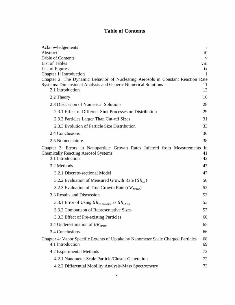
Table of Contents
Acknowledgements i
Abstract iii Table of Contents v List of Tables viii List of Figures ix Chapter 1: Introduction 1
Chapter 2: The Dynamic Behavior of Nucleating Aerosols in Constant Reaction Rate
Systems: Dimensional Analysis and Generic Numerical Solutions 11 2.1 Introduction 12
2.2 Theory 16
2.3 Discussion of Numerical Solutions 28
2.3.1 Effect of Different Sink Processes on Distribution 29
2.3.2 Particles Larger Than Cut-off Sizes 31
2.3.3 Evolution of Particle Size Distribution 33
2.4 Conclusions 36
2.5 Nomenclature 38
Chapter 3: Errors in Nanoparticle Growth Rates Inferred from Measurements in
Chemically Reacting Aerosol Systems 41
3.1 Introduction 42
3.2 Methods 47
3.2.1 Discrete-sectional Model 47
3.2.2 Evaluation of Measured Growth Rate (𝐺𝑅𝑚) 50
3.2.3 Evaluation of True Growth Rate (𝐺𝑅𝑡𝑟𝑢𝑒) 52
3.3 Results and Discussion 53
3.3.1 Error of Using 𝐺𝑅𝑚,𝑚𝑜𝑑𝑒 as 𝐺𝑅𝑡𝑟𝑢𝑒 53
3.3.2 Comparison of Representative Sizes 57
3.3.3 Effect of Pre-existing Particles 60
3.4 Underestimation of 𝐺𝑅𝑡𝑟𝑢𝑒 65
3.4 Conclusions 66
Chapter 4: Vapor Specific Extents of Uptake by Nanometer Scale Charged Particles 68
4.1 Introduction 69
4.2 Experimental Methods 72
4.2.1 Nanometer Scale Particle/Cluster Generation 72
4.2.2 Differential Mobility Analysis-Mass Spectrometry 73
vi
4.3 Results and Discussion 75
4.3.1 Characteristic DMA-MS Mass-Mobility Spectra 75
4.3.2 Inverse Mobility Shifts due to Vapor Adsorption 80
4.3.3 Influence of Charge State 82
4.3.4 Influence of Cluster Size 85
4.3.5 Heterogeneous Vapor Uptake Modelling 86
4.3.6 Sorption and Molecular Structure 90
4.4 Conclusions 91
Chapter 5: Mass, Momentum, and Energy Transfer in Supersonic Aerosol Deposition
Processes 94 5.1 Introduction 95
5.2 Computational Methods 98
5.2.1 Nozzle Geometry and Simulation Domain 98
5.2.2 Computational Fluid Dynamics Simulation 99
5.2.3 Particle Trajectory Simulations 101
5.3 Results & Discussion 105
5.3.1 Simulation results of flow properties 105
5.3.2 Particle Impaction Simulation Results 109
5.3.3 Mass, Momentum and Energy Transfer 115
5.3.3.1 A Framework for Flux Calculations 115
5.3.3.2 Flux Calculations 117
5.4 Conclusions 122
Chapter 6: Differentiation of Normal and Lung Cancer Cell Lines via VOC Profiling with
Proton Transfer Reaction Time-of-Flight Mass Spectrometry 125
6.1 Introduction 126
6.2 Experimental Section 129
6.2.1 Cell Culture Preparation 129
6.2.2 Cell Culture Headspace VOC Sampling 130
6.2.3 PTR-MS Operation 132
6.3 Data Analysis 132
6.3.1 Cell Type Classification 133
6.3.2 Inter-medium Comparison 134
6.4 Results and Discussion 135
6.4.1 PTR-MS Raw Spectra 135
6.4.2 Signal Distribution of Selected Ions 136
vii
6.4.3 Statistical Learning Algorithm Classification & Prediction 140
6.4.4 Predicting Cell Type Cultivated in a Distinct Medium (RPMI) 146
6.5 Conclusions 148
Chapter 7: Conclusions 150
Bibliography 153 Appendix A: Evaluation of Coagulation Effects on Mode Diameter Growth 166 Appendix B: Dimensional Particle Size Distribution 168 Appendix C: Additional Langmuir Model Fitting Results and Mass-mobility Spectra 170 Appendix D: Calculation of Zg 172
Appendix E: Equations for the SST 𝒌 − 𝝎 Turbulent Model 174 Appendix F: Neural Network Fitting of the Particle Drag Coefficient 177
Appendix G: Gas Viscosity and Mean Free Path Calculation 181 Appendix H: Additional Plots of Flow Profile, Knudsen and Mach Numbers and Particle
Trajectories 182
Appendix I: Additional Information of Ion Peaks and Subset Selection 184
viii
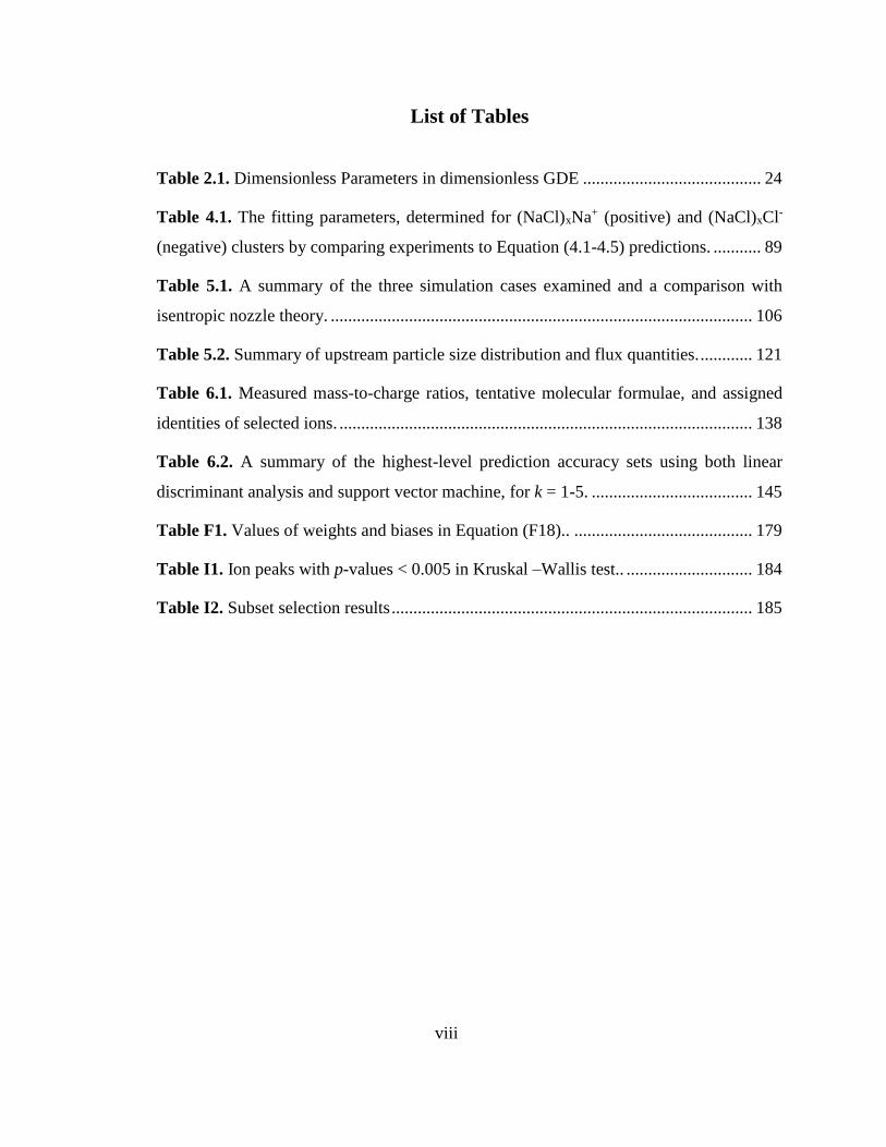
List of Tables
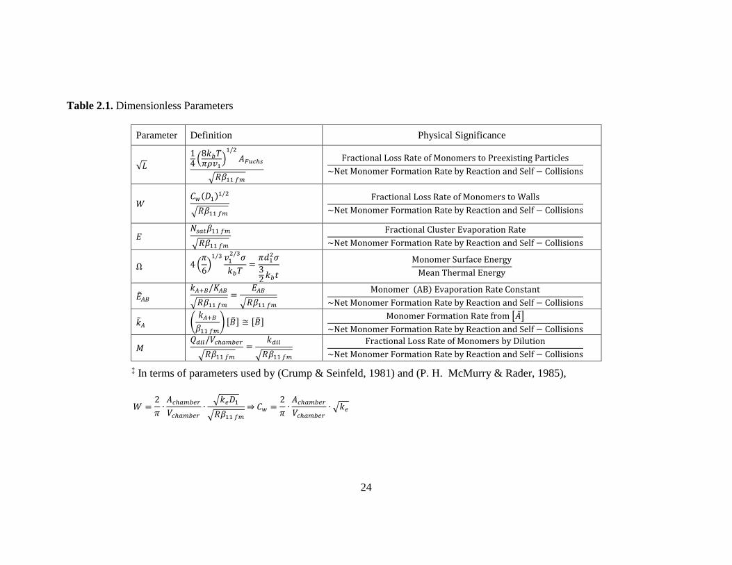
Table 2.1. Dimensionless Parameters in dimensionless GDE ......................................... 24
Table 4.1. The fitting parameters, determined for (NaCl)xNa+ (positive) and (NaCl)xCl-
(negative) clusters by comparing experiments to Equation (4.1-4.5) predictions. ........... 89
Table 5.1. A summary of the three simulation cases examined and a comparison with
isentropic nozzle theory. ................................................................................................. 106
Table 5.2. Summary of upstream particle size distribution and flux quantities. ............ 121
Table 6.1. Measured mass-to-charge ratios, tentative molecular formulae, and assigned
identities of selected ions. ............................................................................................... 138
Table 6.2. A summary of the highest-level prediction accuracy sets using both linear
discriminant analysis and support vector machine, for k = 1-5. ..................................... 145
Table F1. Values of weights and biases in Equation (F18).. ......................................... 179
Table I1. Ion peaks with p-values < 0.005 in Kruskal –Wallis test.. ............................. 184
Table I2. Subset selection results ................................................................................... 185
ix
List of Figures
Figure 1.1. Schematic of the DMA-MS setup. .................................................................. 6
Figure 1.2. A simplified aerosol deposition (AD) setup. ................................................... 7
Figure 2.1. Transition regime vs free molecular regime solutions to the dimensional
equations for collision-controlled nucleation.................................................................... 22
Figure 2.2. Effects of 𝑊, 𝐿, 𝑀, 𝐸 and 𝐸𝐴𝐵 on dimensionless number distributions. ...... 31
Figure 2.3. Effects of dimensionless parameters on time-dependent total concentrations
and maximum concentrations. .......................................................................................... 33
Figure 2.4. Contour plots showing the effects of 𝑊,𝐿,𝑀, 𝐸 and 𝐸𝐴𝐵 on time-dependent
size distributions.. ............................................................................................................. 35
Figure 3.1. Particle size distributions at dimensionless times 𝜏 = 20, 60 ,100. .............. 52
Figure 3.2. 𝑑𝑝,𝑚𝑜𝑑𝑒 and various growth rates as functions of time for collision-controlled
nucleation.. ........................................................................................................................ 54
Figure 3.3. Representative sizes as functions of time and measured growth rates as
functions of representative sizes without preexisting particles......................................... 58
Figure 3.4. Effect of preexisting particles on particle growth rates ................................. 61
Figure 3.5. Representative sizes as functions of time and measured growth rates as
functions of representative sizes with preexisting particles. ............................................. 64
Figure 3.6. Particle size distribution for collision-controlled nucleation ......................... 66
Figure 4.1. Contour plots of mass-mobility spectra for positively charged sodium
chloride cluster ions ((NaCl)x(Na+)z) ................................................................................ 76
Figure 4.2. Contour plots of mass-mobility spectra for negatively charged sodium
chloride cluster ions ((NaCl)x(Cl-)z) ................................................................................. 79
Figure 4.3. Signal intensity-normalized inverse mobility spectra for the singly charged
ions (both positively and negatively charged) at selected vapor pressures ...................... 80
x
Figure 4.4. Inverse mobilities of selected cluster ions as a function solvent partial
pressure. ............................................................................................................................ 84
Figure 4.5. Comparison of sorption of different vapors. ................................................. 86
Figure 5.1. Nozzle geometry and simulation domain ...................................................... 99
Figure 5.2. Fluid flow simulation results for the 3 examined cases............................... 107
Figure 5.3. Particle trajectory simulation results for copper particles for case 1. .......... 110
Figure 5.4. Comparison of impaction speeds of copper and silica particle. .................. 114
Figure 5.5. Normalized test lognormal size distribution functions , calculated mass , x-
direction momentum and kinetic energy fluxes. ............................................................. 119
Figure 6.1. A schematic diagram of the cell chamber used for the VOC sampling
experiments. .................................................................................................................... 131
Figure 6.2. Representative PTR-MS spectra for BEAS-2B (red) and A549 (black) cell lines
......................................................................................................................................... 135
Figure 6.3. Standardized concentration distributions for selected ions. ............................ 139
Figure 6.4. PCA results obtained using the 19 candidate ions selected by the Kruskal-Wallis
test. .................................................................................................................................. 141
Figure 6.5. Highest prediction accuracy as a function of the number of features used in the
classification algorithm for linear discriminant analysis (LDA) and support vector machine
(SVM). ............................................................................................................................. 143
Figure 6.6. The positions of all samples on LDA transformed coordinates. ..................... 148
Figure B1. Dimensional particle size distribution and growth rate. .............................. 169
Figure C1. Langmuir model fitting for (a) (NaCl)xNa+ (x=1, 13) and (b) (NaCl)xCl-
(x=1,4,9,13). .................................................................................................................... 170
Figure C2. Contour plot for positively charged sodium chloride cluster ions at Pc = 48Pa.
......................................................................................................................................... 171
Figure F1. Comparison between DSMC results and Henderson’s correlation. ............. 177
xi
Figure F2. (a) Comparison of the drag coefficient given by equation (F1) with
experimental data, simulated results (obtained by DSMC) and theoretical values in the
free molecular limit. ........................................................................................................ 179
Figure H1. Contour plots of Mach number, static pressure, temperature and density of
the carrier gas (N2) at operating conditions of 760 Torr inlet pressure and 10 Torr outlet
pressure. .......................................................................................................................... 182
Figure H2. (a) The Knudsen numbers of particles traversing along the symmetry line for
case 1 (copper particles). (b) The relative particle velocity to speed of sound ratio of
copper particles traversing along the symmetry line case 1. .......................................... 183
Figure H3. Particle trajectories for particles with diameter (a) 𝑑𝑝=10 𝑛𝑚, (b) 𝑑𝑝=1 𝜇𝑚 and
(c) 𝑑𝑝=10 𝜇𝑚. ................................................................................................................. 183
1
Chapter 1: Introduction
Particle nucleation and growth in the gas phase play an important role in a variety
of systems. In general, nucleation occurs via chemical reaction of gas phase precursors;
this produces condensable species with low vapor pressure, which can be homogeneous
or, more commonly, heterogeneous in chemical composition. Collisions between
condensable species lead to gas-to-particle phase transition (nucleation) and subsequent
collisions of condensable species with formed particles leads to particle growth
(condensation). For example, in the atmosphere, oxidation of sulfur dioxide and volatile
organic compounds produces condensable sulfuric acid and highly oxygenated organic
molecules (Kirkby, 2011; Tröstl et al., 2016) that are partially responsible for new
particle formation and particle growth in the atmosphere. These particles are a major
source of pollution, affecting both climate (through their influence on cloud formation)
(Seinfeld & Pandis, 2016) and human health. In hydrocarbon combustion, undesirable
soot particles are produced by incomplete oxidation of the hydrocarbon fuel. Soot
formation occurs by a very similar process, wherein hydrocarbons react to form
condensable species, leading to soot nucleation and growth. Soot (black carbon) is a
known carcinogen and with documented deleterious effects on human health (Haynes &
Wagner, 1981; Shiraiwa, Selzle, & Pöschl, 2012) . Conversely, vapor phase
organometallic precursors can be injected into combustion and high temperature reactors
for the synthesis of functional particles, incorporated into catalysts, sensors, biomaterials
and electroceramics (Strobel & Pratsinis, 2007). Hereto, the vapor phase precursors react
to form condensable species. In all such systems, it is thus important to understand the
2
interplay between the formation of condensable species, nucleation, and subsequent
condensational particle growth, as well as with other dynamics affecting particle size
distribution functions, namely deposition and coagulation.
This dissertation focuses on the dynamics of particles in the gas phase in a general
manner and contains five sub-studies. The first two focus on the development and
implementation of discrete-sectional models to better describe the interplay between
condensable species formation, nucleation, condensation, coagulation, and particle
deposition in experimental systems intended to mimic new particle formation in the
atmosphere. The third is devoted the implementation of novel ion mobility-mass
spectrometry based methods of probing condensation at the molecular scale, i.e.
experimentally detecting vapor molecule binding to nanometer scale clusters. The fourth
focuses on the development of new models to describe particle transport in variable
Knudsen number, variable Mach number environments, and the application of such
models in designing particle based coating process. Finally, the fifth focuses on the use
of proton transfer reaction mass spectrometry to detect biologically derived volatile
organic carbonaceous material (VOCs). Though each of these works is distinct in its
motivation and each is written as a standalone manuscript, they are connected through
their focus on the dynamics of particle and vapor laden gas phase systems. The
remainder of this introductory chapter is devoted to a description of background material
relevant to all chapters, including the modeling equations utilized in the first two studies,
the instrumentation in the ion mobility-mass spectrometry focused work, a description of
scenarios wherein aerosols are in variable Mach number, variable Knudsen number
flows, and a brief overview on the detection of biologically derived VOCs.

3
The simplest particle nucleation and growth scenario occurs when there is "zero
activation energy" (or ‘spinodal decomposition’). In this scenario, molecules/clusters of
the condensing species merge into a new particle upon colliding and evaporation from
particle surface is negligible compared to particle formation rates. This is the fastest
route for particle nucleation (referred to as the ‘collision-controlled limit’ hereafter) and
can be accurately modeled provided particle kinetics are correctly described. It has been
reported that in multiple systems, e.g. particle formation in a chamber that contains a
mixture of sulfuric acid and dimethylamine (Kürten et al., 2018), toluene vapor
nucleation in a converging diverging nozzle (Chakrabarty, Ferreiro, Lippe, & Signorell,
2017), particle nucleation does approach the collision-controlled limit. However, a
number of physical and chemical processes, e.g. evaporation from particle surface,
particle deposition on reactor walls, system dilution, surface/volume chemical reactions,
can cause the particle formation and growth processes to deviate significantly from the
collision-controlled limit. The general dynamic equations (GDE) is a set of first order
differential equations that integrate all these processes. For concentrations of particles
with size 𝑑𝑝, the continuous form of the GDE can be written as:
𝑑𝑛(𝑑𝑝, 𝑡)
𝑑𝑡= −
𝜕
𝜕𝑑𝑝
(𝐼(𝑑𝑝, 𝑡)𝑛(𝑑𝑝 , 𝑡)) +1
2∫ 𝛽(𝑑𝑝
′ , 𝑑𝑝 −𝑑𝑝
0
𝑑𝑝′ )𝑛(𝑑𝑝
′ , 𝑡)𝑛(𝑑𝑝−𝑑𝑝′ )𝑑𝑑𝑝 −
∫ 𝛽(𝑑𝑝′ , 𝑑𝑝
∞
0)𝑛(𝑑𝑝
′ , 𝑡)𝑛(𝑑𝑝)𝑑𝑑𝑝 − 𝑆𝑖𝑛𝑘(𝑑𝑝, 𝑡)𝑛(𝑑𝑝, 𝑡) + 𝑆𝑜𝑢𝑟𝑐𝑒(𝑑𝑝 , 𝑡)𝑛(𝑑𝑝, 𝑡) (1.1)
where 𝑛(𝑑𝑝, 𝑡) is the concentration of particles with diameter 𝑑𝑝 at time 𝑡, 𝐼(𝑑𝑝, 𝑡) =
𝑑𝑑𝑝
𝑑𝑡 is the particle growth rate due to net molecular uptake processes (condensation,
evaporation, surface or volume chemical reactions). The two integral terms in Equation
(1.1) represent particle formation and loss due to particle coagulation, respectively.
4
𝑆𝑖𝑛𝑘(𝑑𝑝) is a generalized term that accounts for particle loss by wall deposition, dilution
or deposition on preexisting aerosols; 𝑆𝑜𝑢𝑟𝑐𝑒(𝑑𝑝) describes the production of particles
with diameter 𝑑𝑝 by other sources. By incorporating different physical/chemical
processes into the GDE, the effect of these processes can be quantitatively evaluated.
Moreover, the GDE can be transformed into dimensionless formulations (Peter H.
McMurry, 1980) that give generalized solutions. To understand the effect of the particle
sink processes and acid-base reaction on particle formation and growth, a discrete-section
form of the GDE is non-dimensionalized in Chapter 2 for a system wherein a single
condensing species is produced at a constant rate, R. The solutions obtained are only
dependent on a set of dimensionless parameters that characterize the relative strength of
sink processes/acid-base reaction and R.
Provided the physics and chemistry within the system are well understood (i.e. all
rate coefficients are known), the GDE provides a bottom-up approach to predict particle
formation and growth. In practice, however, the concentration of the condensing species,
a key quantity in solving the GDE, is often unknown and can prove difficult to measure.
In these circumstances, the concentration of condensing species must be determined
indirectly from experimentally measurable quantities, i.e. particle growth rates. Multiple
methods have been developed for this purpose (Markku Kulmala et al., 2012), e.g. the
maximum concentration method, the log-normal distribution function method. One
common feature shared by these methods is that a specific particle size is chosen to
represent the experimentally measured particle size distribution (the local concentration
maximum of the nucleation mode, for example); the particle growth rate is then

5
calculated by following the evolution of this size as a function of time. Implicitly
assumed in this approach is that molecular uptake of the nucleating species is the major
contributor to the calculated growth rate, while the effects of coagulation and particle
sink terms are not explicitly accounted for. As a result, the growth rate calculated in this
manner may deviate from the true particle growth rate due to net molecular uptake
processes, from which information regarding the condensing species can be extracted. In
Chapter 3, this deviation is systematically examined and the limit of error is calculated
for certain nucleation scenarios.
One special case of particle growth, which is of particular interest for particle
detection, is particle growth in a condensational particle counter (CPC). In a CPC,
particles are exposed to a supersaturated vapor (e.g. butanol, water). The vapor condenses
heterogeneously on the particle surface and further condensation leads the particles to
grow to an optically detectable size (M. R. Stolzenburg & McMurry, 1991). For particles
with mobility diameters greater than 3 nm, the activation efficiency (defined as the
fraction of grown particles to the total number of particles admitted into the growth tube
in the CPC) of commercially available CPCs can reach ~100%. However, for sub-3 nm
particles, it has been found that the CPC detection efficiency is highly dependent on
particle size, polarity and composition (Iida, Stolzenburg, & McMurry, 2009; Chongai
Kuang, Chen, McMurry, & Wang, 2012). Understanding the origin of these dependencies
would provide insights into the heterogeneous nucleation process as well as assist novel
CPC design.
Condensational growth of particles in a CPC starts with vapor sorption on the
particle surface. At the University of Minnesota, it has been demonstrated that a
6
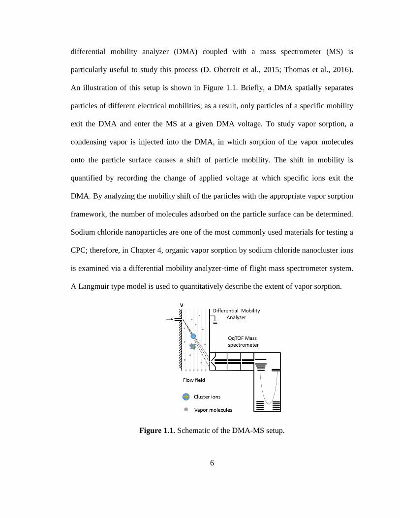
differential mobility analyzer (DMA) coupled with a mass spectrometer (MS) is
particularly useful to study this process (D. Oberreit et al., 2015; Thomas et al., 2016).
An illustration of this setup is shown in Figure 1.1. Briefly, a DMA spatially separates
particles of different electrical mobilities; as a result, only particles of a specific mobility
exit the DMA and enter the MS at a given DMA voltage. To study vapor sorption, a
condensing vapor is injected into the DMA, in which sorption of the vapor molecules
onto the particle surface causes a shift of particle mobility. The shift in mobility is
quantified by recording the change of applied voltage at which specific ions exit the
DMA. By analyzing the mobility shift of the particles with the appropriate vapor sorption
framework, the number of molecules adsorbed on the particle surface can be determined.
Sodium chloride nanoparticles are one of the most commonly used materials for testing a
CPC; therefore, in Chapter 4, organic vapor sorption by sodium chloride nanocluster ions
is examined via a differential mobility analyzer-time of flight mass spectrometer system.
A Langmuir type model is used to quantitatively describe the extent of vapor sorption.
Figure 1.1. Schematic of the DMA-MS setup.

7
Nucleated particles, either formed in the liquid or gas phase, can be collected for
manufacturing purposes. In Chapter 5, this dissertation discusses one method that has
been increasingly adopted for surface coating and thin film production via impacting
particles on a substrate, i.e. the aerosol deposition technique (AD) (Akedo, 2006; Jun &
Maxim, 2002). In AD, micron or submicron scale particles are accelerated to exceed the
speed of sound to impact on a substrate, facilitating formation of compact films. To
achieve high particle impaction speed, converging-diverging nozzles are often utilized to
generate a supersonic flow field. Figure 1.2 shows an illustrative schematic of an AD
setup.
Figure 1.2. A simplified aerosol deposition (AD) setup. The upstream working pressure
for AD is close to ambient pressure and the downstream pressure is typically several torr.
A shockwave forms close to the substrate since the incoming flow to the substrate is
supersonic.
8
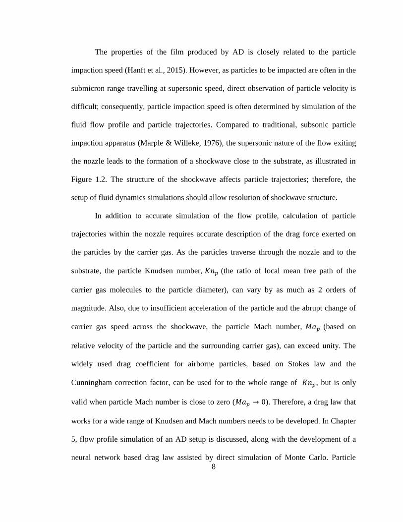
The properties of the film produced by AD is closely related to the particle
impaction speed (Hanft et al., 2015). However, as particles to be impacted are often in the
submicron range travelling at supersonic speed, direct observation of particle velocity is
difficult; consequently, particle impaction speed is often determined by simulation of the
fluid flow profile and particle trajectories. Compared to traditional, subsonic particle
impaction apparatus (Marple & Willeke, 1976), the supersonic nature of the flow exiting
the nozzle leads to the formation of a shockwave close to the substrate, as illustrated in
Figure 1.2. The structure of the shockwave affects particle trajectories; therefore, the
setup of fluid dynamics simulations should allow resolution of shockwave structure.
In addition to accurate simulation of the flow profile, calculation of particle
trajectories within the nozzle requires accurate description of the drag force exerted on
the particles by the carrier gas. As the particles traverse through the nozzle and to the
substrate, the particle Knudsen number, 𝐾𝑛𝑝 (the ratio of local mean free path of the
carrier gas molecules to the particle diameter), can vary by as much as 2 orders of
magnitude. Also, due to insufficient acceleration of the particle and the abrupt change of
carrier gas speed across the shockwave, the particle Mach number, 𝑀𝑎𝑝 (based on
relative velocity of the particle and the surrounding carrier gas), can exceed unity. The
widely used drag coefficient for airborne particles, based on Stokes law and the
Cunningham correction factor, can be used for to the whole range of 𝐾𝑛𝑝, but is only
valid when particle Mach number is close to zero (𝑀𝑎𝑝 → 0). Therefore, a drag law that
works for a wide range of Knudsen and Mach numbers needs to be developed. In Chapter
5, flow profile simulation of an AD setup is discussed, along with the development of a
neural network based drag law assisted by direct simulation of Monte Carlo. Particle
9
trajectory simulation results and subsequent calculation of mass, momentum and heat
transfer rates from particles to the substrate are also presented in Chapter 5.
In Chapter 6, a molecular perspective is taken to explore the possibility of disease
diagnosis based on volatile organic compound (VOC) detection and quantification
(referred as ‘VOC profiling’ hereafter), using techniques more commonly used in
monitoring gas species concentrations in atmospheric systems. Biological samples, in
vitro and in vivo, can emit a rich body of volatile organic compounds that serve as the
samples’ biological signature. Therefore, in principle, the biological samples can be
classified and sample types be predicted through VOC profiling. Due to the non-intrusive
nature of VOC sampling processes, the potential of VOC profiling as a transformative
diagnostic technique has long been recognized by researchers (Haick, Broza, Mochalski,
Ruzsanyi, & Amann, 2014; Hakim et al., 2012). Common techniques of VOC profiling
include gas chromatography-mass spectrometry (GC-MS) (Ligor et al., 2008; Wojciech
et al., 2014), proton transfer reaction-mass spectrometry (PTR-MS) (Brunner et al., 2010;
Tali et al., 2016) and a wide variety of nanosensors (Di Natale et al., 2003; Machado et
al., 2005; G. Peng et al., 2010).
VOC profiling results need to be coupled with proper data processing techniques
to enable robust, and even automated disease diagnosis. Machine learning algorithms are
designed to learn from existing data and make predictions with incoming data. As a result,
learning algorithms such as principle component analysis, discriminant analysis, decision
trees are often utilized to analyze biological datasets. In Chapter 6, a PTR-MS is utilized
to profile VOCs emitted by in vitro lung cancer cells as well as normal lung cells.
10
Selected machine learning algorithms are then applied to process the PTR-MS
measurement data to classify and predict cell types.
In total, my dissertation mainly discusses particle formation, growth and transport
on the molecular and nano- scales. As a summary of this introduction, my dissertation is
structured as follows:
Chapter 2 focuses on the effect of different particle sink processes and acid-base
reactions on particle size distribution for a constant reaction rate system. A
dimensionless framework is formulated and the GDE is numerically solved with
a discrete sectional model.
Chapter 3 discusses the errors associated with methods commonly employed for
the calculation of particle growth rates using experimental data.
Chapter 4 examines organic vapor sorption by sodium chloride cluster ions by a
tandem differential mobility analyzer-mass spectrometer (DMA-MS) setup.
Quantitative analysis is performed with a Langmuir type model to determine the
extent of vapor uptake.
Chapter 5 presents simulation results for an aerosol deposition process with a slit
type converging diverging nozzle. A neural network based drag law that
facilitates particle trajectory calculations is developed. Size and density
dependent particle transport process is described. A framework that can be used
for mass, momentum and heat transfer from the particles to the substrate is
formulated.
Chapter 6 discusses lung cancer cell classification and prediction facilitated by
PTR-MS based VOC profiling and machine learning data analysis techniques.
11
Chapter 2: The Dynamic Behavior of Nucleating Aerosols in Constant
Reaction Rate Systems: Dimensional Analysis and Generic Numerical
Solutions
Abstract: Aerosol particles are formed by chemical transformations in diverse
systems including the atmosphere, fossil fuel combustors, aerosol synthesis reactors,
and semiconductor processing equipment. This study discusses solutions to the
aerosol population balance equations that account for nucleation, coagulation, wall
deposition, scavenging by preexisting particles, and dilution with particle-free air in
spatially homogeneous systems when a condensing species is produced by gas phase
reactions at a constant rate. Two nucleation mechanisms are considered: classical
nucleation due to competing rates of condensation and evaporation, and chemical
nucleation due to acid-base reactions. The equations, which apply to a single
component system (two components, the acid and base, are included for acid-base
nucleation), are cast in a dimensionless form. This leads to dimensionless
parameters (dimensionless rate constants) that characterize the importance of each
process. When these parameters are sufficiently small, the corresponding process
(scavenging by pre-existing particles, wall deposition, dilution, and cluster
evaporation) has an insignificant effect and nucleation approaches the collision-
controlled limit. Because the dimensionless parameters vary inversely with the
square root of the reaction rate, the collision-controlled limit is reached for any
chemical system provided the reaction rate is high enough. The numerical solutions
quantify the effects of each process for low rates of gas-to-particle conversion where
12
the dimensionless parameters become sufficiently large. They also illustrate how
data for sub 10 nm number distributions can provide insights into the nucleation
process.
2.1 Introduction
Certain gases react to produce nonvolatile particulate products. For example, in
the atmosphere, sulfur dioxide (SO2) reacts with hydroxyl to form sulfates, and complex
reaction pathways involving many organic precursors can also lead to particle formation
(Kirkby et al., 2016; Seinfeld & Pandis, 2016; Tröstl et al., 2016). Silane and other gases
react to form contaminant particles in semiconductor processing equipment (Swihart &
Girshick, 1999), and titanium tetrachloride is used to produce catalytic particles in flame
synthesis reactors (Koirala, Pratsinis, & Baiker, 2016). In such systems, particles can
nucleate from trace gas phase constituents formed by chemical reaction and can
subsequently grow by condensation and coagulation. Other processes, such as loss to
preexisting particles, deposition on reactor walls, entrainment of particle free air, cluster
evaporation, etc. can also affect the number distributions of the nucleated aerosol. This
study discusses solutions to the aerosol population balance equations pertinent to such
processes.
There is a rich and growing body of work aimed at understanding the detailed
chemical processes responsible for aerosol formation in reacting systems. This work
shows that multiple species often contribute, and that particle mass can be formed by
reactions that occur in the gas phase and on or within particles. Rather than attempting to
describe the behavior of a particular system in all its complexity, the objective of this
13
study is to obtain general solutions constrained by well-defined simplifying assumptions.
In particular, we assume that only a single chemical species contributes to particle
formation (two species, sulfuric acid and a basic gas, are considered for acid-base
nucleation), and that this species is formed at a constant rate R [molecules cm−3 s−1] .
These may be good assumptions for aerosol formation in some chemical systems, such as
the nucleation of sulfuric acid with a strong basic gas. For chemically more complex
systems, such as atmospheric secondary organic aerosols, deviations between
observations and our theoretical predictions may provide some insight into types of
processes that are important.
This study builds on early work by Peter H. McMurry, beginning with McMurry
(1980). That work focused on interpreting the pioneering measurements done by William
Clark (W. E. Clark, 1972; W. E. Clark & Whitby, 1975), a doctoral student of the late
Prof. Kenneth T. Whitby. Using the Whitby Aerosol Analyzer (WAA) (Whitby & Clark
1966), Clark measured time-dependent size distributions of 4 400 nm aerosol particles
formed photochemically from SO2 in a 17.7 m3 Teflon film reactor. Although the air
used in these experiments almost certainly contained unmeasured organic contaminants
that contributed to aerosol formation, sulfates probably dominated since the
concentrations of SO2 were very high (49-2,880 ppb). It probably also contained
significant concentrations of stabilizing compounds, such as ammonia or amines.
McMurry's analysis assumed that a single chemical species was responsible for
nucleation and particle growth. While McMurry (1980) accounted for all possible cluster
and particle coagulation interactions, he assumed that evaporation rates were negligible
relative to condensation rates (i.e., that nucleation was "collision-controlled").
14
Furthermore, he showed that if a single condensing species is formed at a constant rate 𝑅,
the population balance equations can be cast in a nondimensional form that is
independent of 𝑅 . With these simplifications McMurry was able to predict observed
number distributions and concentrations with to within about 50%. This "zero activation
energy" approach (referred to as "spinodal decomposition" by the nucleation community)
greatly simplifies nucleation modeling, since the primary uncertainties in nucleation
theory involve modeling cluster stability (evaporation rates). Recent work from the
CLOUD consortium involving the photooxidation of SO2 in the presence of dimethyl
amine (DMA) showed that "neutral clusters containing up to 14 SA [sulfuric acid] and 16
DMA molecules form at or close to the kinetic limit, limited only by the collision rate of
SA molecules" (Kurten et al., 2014), confirming McMurry's 1980 hypothesis.
Atmospheric observations also show that particle formation rates often vary in proportion
to [H2SO4]2 (C. Kuang, McMurry, McCormick, & Eisele, 2008; Weber et al., 1996), a
result consistent with collision-controlled nucleation. Sihto (2006) and Riipinen (2007)
found that particle formation rates vary as [H2SO4]p (1<p<2), which led to their
conclusion that nucleation may either be limited by collisions of sulfuric acid with itself
(p=2) or with an organic compound (p=1). Our analysis in this study does not address the
latter possibility.
Rao and McMurry(1989) incorporated wall losses of sulfuric acid "monomer" and
nanometer-sized particles in the nondimensional framework described above. Diffusion-
limited wall deposition rates of these small particles were determined using the theory
developed by Crump and Seinfeld (1981) and widely used by others including Kurten et
al. (2014). They also accounted for cluster evaporation, assuming that evaporation rates
15
could be predicted with the Kelvin equation (e.g., Friedlander (2000)). This allowed them
to study the transition from collision-controlled to condensation/evaporation-controlled
nucleation. In this study, our treatment of wall losses and classical
condensation/evaporation-controlled nucleation is identical to that introduced by Rao and
McMurry (1989), although our analysis is expanded to include other processes that might
occur simultaneously. Independently, Lushnikov and Kulmala (1995) described a
nondimensional solution for "source-enhanced" classical nucleation that accounted for
the chemical production of condensing vapor. Their analysis was formulated to account
for time-dependent vapor formation rates, so it follows that their analytical solutions are
also applicable to constant rate systems. Their analysis also assumes constant
condensation coefficients, which is not applicable to atmospheric nucleation, and does
not account for cluster coagulation or other cluster removal processes.
Since about 1990, we and others have focused on developing new instruments for
measuring clusters and particles in the 1 nm range together with their gas phase
precursors (especially sulfuric acid vapor). These instruments have been used for
atmospheric observations and laboratory experiments. This work has shown that acid-
base nucleation is one process that contributes to nucleation in the atmosphere. Also, in
some studies (e.g., CLOUD) experiments are done using constant volume reactors with
sampled air continuously replenished with particle-free flow. This study incorporates
these processes into the dimensionless framework from the 1980s and systematically
compares the effects of each process on the dynamic behavior of the nucleated aerosols.
This work complements the detailed understanding of cluster chemistry that has been the
focus of much recent work, as it provides a means to confirm closure between predicted
16
and observed number distributions of larger particles. It is those larger particles that
determine the properties or effects of the nucleated aerosol.
2.2 Theory
We assume that a single condensing species is produced by gas phase chemical
reactions at a constant rate 𝑅 [molecules cm−3 s−1], and we consider two nucleation
scenarios: (i) single component nucleation accounting for cluster evaporation using the
classical liquid droplet model, and (ii) chemical nucleation by reactions of sulfuric acid
vapor with a basic gas (e.g., ammonia or an amine). For both scenarios, species
concentrations are assumed to be spatially uniform, all possible coagulation interactions
are included, particles are assumed spherical, and time-dependent (rather than steady-
state) solutions are obtained. We begin with the dimensional equations for both
nucleation scenarios followed by their dimensionless analogs. The reader is referred to
the nomenclature for definitions and some important relationships.
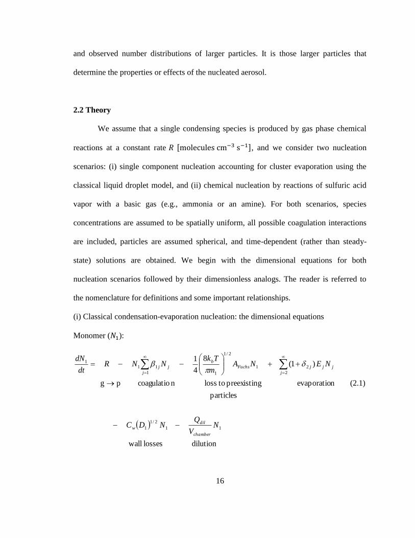
(i) Classical condensation-evaporation nucleation: the dimensional equations
Monomer (𝑁1):
dilution losses wall
particles
(2.1)n evaporatio gpreexistin toloss n coagulatio pg
)1( 8
4
1
11
2/1
1
2
21
2/1
11
111
NV
QNDC
NENAm
TkNNR
dt
dN
chamber
dil
w
jj
j
jFuchs
b
j
jj

17
Clusters (𝑁𝑘, 𝑘 > 2):
dilution losses wall n evaporatio
particles
(2.2) gpreexistin toloss n coagulatio
8
4
1
2
1
2/1
11
2/1
11
k
chamber
dilkkwkkkk
kFuchsb
j
j
kjkj
kji
iijk
NV
QNDCNENE
NAkm
TkNNNN
dt
dN
In Equation (2.2), k corresponds to the number of vapor molecules (monomer) in
a cluster, and is used both as a subscript and a variable (third term on r.h.s.). This
formulation implicitly assumes two populations of particles: those formed by nucleation,
which are included in the coagulation terms, and those present initially (𝐴𝐹𝑢𝑐ℎ𝑠). The
coagulation terms in these equations are discussed in textbooks (e.g., (Friedlander, 2000;
Seinfeld & Pandis, 2016). The evaporation rate constants, 𝐸𝑗 , are derived using
assumptions of the classical liquid droplet model, and are expressed in a discretized form
that accounts for the evaporation of one molecule from a size j cluster to form a size j-1
cluster as well as the relative motion of the monomer and evaporating clusters (see
nomenclature). In the limit of large j, 3
2(𝑗2/3 − (𝑗 − 1)2/3) → 𝑗−1/3 and the cluster size
dependence in our expression for 𝐸𝑗 (see nomenclature) collapses to the usual Kelvin
equation expression. The Kelvin equation is derived assuming that the Gibbs free energy
change for droplet formation is a continuous function of droplet radius, an approximation
that becomes increasingly inaccurate as j decreased below 10. Our discrete formulation
18
does nothing to ensure the validity of the underlying physical assumptions that lead to the
liquid droplet model and has only a small effect on calculated results. The wall loss term
is of the form used by Kurten et al. (2014). The relationship between this and earlier
notation is shown in the footnote to Table 2.1. The empirical constant, 𝐶𝑤 , is
independent of particle size, but depends on the reactor dimensions and operating
conditions (i.e., convection, temperature, etc.). The dilution term accounts for the
entrainment of particle-free air, and assumes that mixing is instantaneous so that
concentrations remain spatially uniform. The terms that describe loss to pre-existing
particles account for transport to particles in the transition regime; the Fuchs surface area
concentration, 𝐴𝐹𝑢𝑐ℎ𝑠, is assumed constant and is based on the approximate expression
given by Fuchs and Sutugin (1971) and discussed by Davis et al. (1981). The relationship
between 𝐴𝐹𝑢𝑐ℎ𝑠 and the condensation sink (CS) used by (Kerminen & Kulmala, 2002) to
describe cluster scavenging by pre-existing particles is (C. Kuang, Riipinen, Sihto, et al.,
2010; P. H. McMurry et al., 2005):
𝐶𝑆 = (8𝑘𝑏𝑇
𝜋𝑚1)1/2 𝐴𝐹𝑢𝑐ℎ𝑠
4 (2.3)
so these approaches are equivalent. This approach for scavenging by preexisting particles
was first discussed by McMurry and Friedlander (P.H. McMurry & Friedlander, 1979);
McMurry (1983) obtained accurate numerical solutions to quantify its effects. Rao and
McMurry (1989) studied evaporation and wall losses using the mathematical framework
discussed above.
(ii) Acid-base nucleation: the dimensional equations

19
The analysis uses the acid-base nucleation model proposed by Jen et al. (2014)
(scheme 2 with 𝐸3 = 0 ). This model involves simplifying assumptions about the
multitude of acid-base reactions that contribute to cluster formation, as exemplified by
the ACDC model proposed by McGrath et al. (2012), and is consistent with laboratory
measurements reported by Jen and coworkers. The reader is referred to Jen's paper for
details. The model for acid-base reactions does not explicitly account for temperature or
for the role of water. Instead, the model assumes that dependencies on those variables
would be reflected primarily in the monomer (𝑁1 = 𝐴𝐵) evaporation rate constant (𝐸𝐴𝐵).
Furthermore, this analysis assumes that the base concentration, [B], remains constant
during nucleation. With these assumptions, Jen's scheme 2 leads to the following
conservation equations for free acid, monomer, and clusters:
Free Acid (A)
dilution losses wall Bith reaction w
]A[ ] A[ ] ][[
(2.4) of particles 1)( clusters all
nevaporatio gpreexistin toloss ith reaction w pg
] A[8
4
1 ] [
][
2/1
1
1
2/1
1
chamber
dil
AwBA
ABFuchs
A
b
j
jAj
V
QDCBAk
ABNj
NEAm
TkNAR
dt
Ad
Monomer (𝑁1 = 𝐴𝐵)

20
B +A forms N forms
dilution losses n wallevaporatio ABA ith reaction w
] A[
B forms particles
(2.5) reaction B+A gpreexistin toloss n coagulatio
] B][A[ 8
4
1
2
11
2/1
1111
1
1
2/1
11
111
NV
QNDCNEN
NA
kNAm
TkNN
dt
dN
chamber
dilwABA
BAFuchsb
j
j
j
Clusters (𝑁𝑘, 𝑘 > 2)
dilution losses wallA with reactions
] A[
particles
(2.6) gpreexistin toloss n coagulatio
8
4
1
2
1
2/1
11
2/1
11
k
chamber
dil
kkwkkAkAk
kFuchs
b
j
j
kjkj
kji
iij
k
NV
QNDCNN
NAkm
TkNNNN
dt
dN
For a constant rate system (R=constant), the above conservation equations for
both nucleation scenarios collapse to a dimensionless form that is independent of R and
of the condensing species' properties (molecular volume, surface tension, mass, etc.)
provided that the collision frequency function is a homogeneous function of those
properties. Particles formed in chambers can easily grow into the transition regime, and
the transition regime collision frequency function is not a homogeneous function of
condensing species properties. However, the free molecular collision frequency function
is homogeneous. Therefore, prior to nondimensionalizing the equations, 𝛽𝑖𝑗 is replaced
with 𝛽𝑖𝑗 𝑓𝑚 , thereby ensuring that solutions to the dimensionless equations are
21
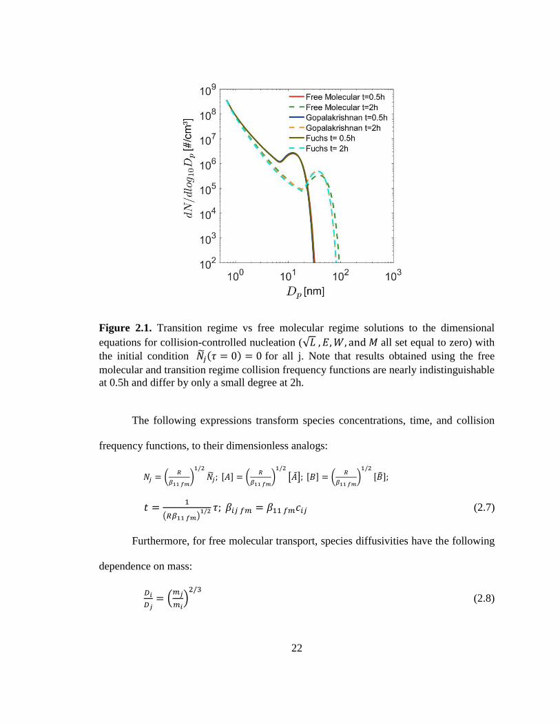
independent of species properties. One might guess that this would significantly limit the
applicability of our results. However, as is shown in Figure 2.1, simulations performed
using free molecular and transition regime collision frequency functions are nearly
indistinguishable at t =0.5h and have only a minor difference at t = 2h. Two approaches
were used for calculating transition-regime coagulation rates: the widely-used expression
developed by Sutugin and Fuchs and described by Fuchs (1964), and the approach
developed by Gopalakrishnan and Hogan (2011). Results obtained using the free
molecular and transition regime collision frequency functions probably agree so well
because most coagulation involves the smallest particles, which are present in much
higher concentrations than particles in the transition regime. The results in Figure 2.1
were obtained assuming a monomer formation rate 𝑅 = 4 × 106 cm−3s−1 and a
monomer volume of 1.62 × 10⁻²² cm3. This reaction rate is high enough to ensure that
aerosol grows into the transition regime during the course of an hour or two; the
monomer volume corresponds to a monomer containing one dimethylamine and one
sulfuric acid molecule with an assumed density of 1.47 g/cm3 We conclude therefore,
that for the chemical nucleation problems addressed in this study, sufficiently accurate
results are obtained with the free molecular expression.
22
Figure 2.1. Transition regime vs free molecular regime solutions to the dimensional
equations for collision-controlled nucleation (√𝐿 , 𝐸,𝑊, and 𝑀 all set equal to zero) with
the initial condition ��𝑗(𝜏 = 0) = 0 for all j. Note that results obtained using the free
molecular and transition regime collision frequency functions are nearly indistinguishable
at 0.5h and differ by only a small degree at 2h.
The following expressions transform species concentrations, time, and collision
frequency functions, to their dimensionless analogs:
𝑁𝑗 = (𝑅
𝛽11 𝑓𝑚)1/2
𝑁𝑗; [𝐴] = (𝑅
𝛽11 𝑓𝑚)1/2
[��]; [𝐵] = (𝑅
𝛽11 𝑓𝑚)1/2
[��];
𝑡 =1
(𝑅𝛽11 𝑓𝑚)1/2 𝜏; 𝛽𝑖𝑗 𝑓𝑚 = 𝛽11 𝑓𝑚𝑐𝑖𝑗 (2.7)
Furthermore, for free molecular transport, species diffusivities have the following
dependence on mass:
𝐷𝑖
𝐷𝑗= (
𝑚𝑗
𝑚𝑖)2/3
(2.8)
23
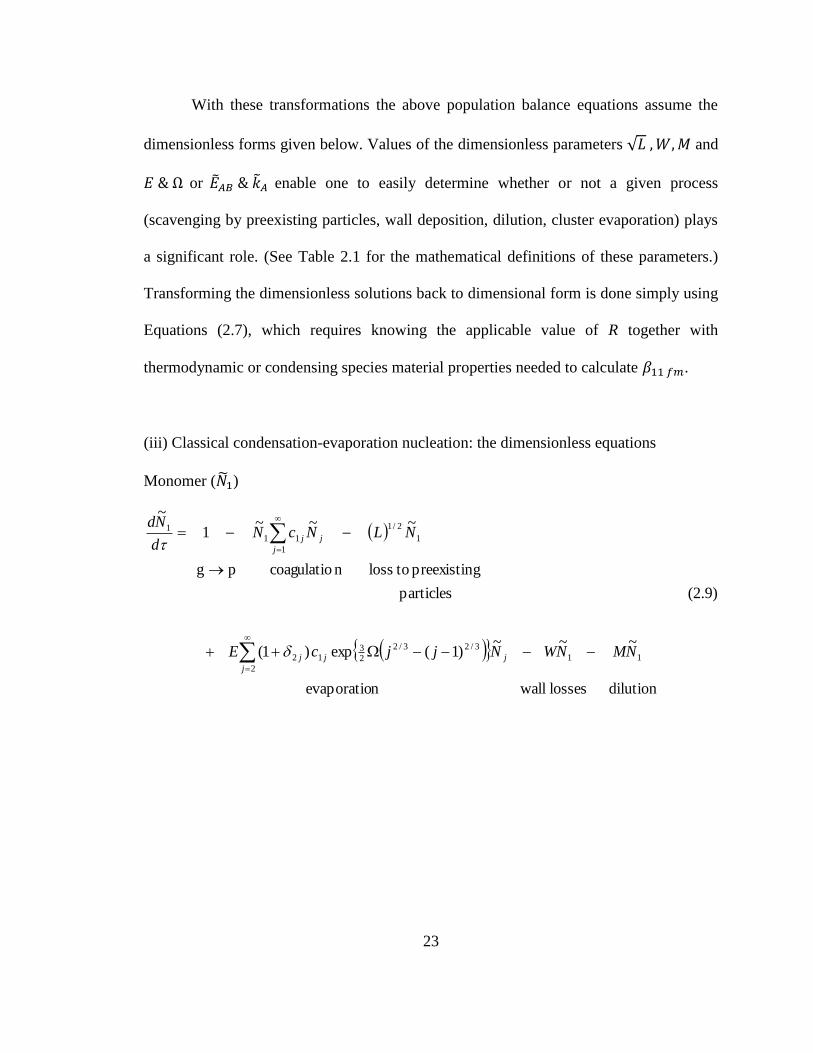
With these transformations the above population balance equations assume the
dimensionless forms given below. Values of the dimensionless parameters √𝐿 ,𝑊,𝑀 and
𝐸 & Ω or ��𝐴𝐵 & ��𝐴 enable one to easily determine whether or not a given process
(scavenging by preexisting particles, wall deposition, dilution, cluster evaporation) plays
a significant role. (See Table 2.1 for the mathematical definitions of these parameters.)
Transforming the dimensionless solutions back to dimensional form is done simply using
Equations (2.7), which requires knowing the applicable value of R together with
thermodynamic or condensing species material properties needed to calculate 𝛽11 𝑓𝑚.
(iii) Classical condensation-evaporation nucleation: the dimensionless equations
Monomer (��1)
dilution losses all w nevaporatio
~
~
~)1(exp )1(
(2.9) particles
gpreexistin tolossn coagulatio pg
~
~~
1
~
11
3/23/2
23
1
2
2
1
2/1
1
111
NMNWNjjcE
NLNcNd
Nd
jj
j
j
j
jj
24
Table 2.1. Dimensionless Parameters
Parameter Definition Physical Significance
√𝐿
14(8𝑘𝑏𝑇𝜋𝜌𝑣1
)1/2
𝐴𝐹𝑢𝑐ℎ𝑠
√𝑅𝛽11 𝑓𝑚
Fractional Loss Rate of Monomers to Preexisting Particles
~Net Monomer Formation Rate by Reaction and Self − Collisions
𝑊 𝐶𝑤(𝐷1)
1/2
√𝑅𝛽11 𝑓𝑚
Fractional Loss Rate of Monomers to Walls
~Net Monomer Formation Rate by Reaction and Self − Collisions
𝐸 𝑁𝑠𝑎𝑡𝛽11 𝑓𝑚
√𝑅𝛽11 𝑓𝑚
Fractional Cluster Evaporation Rate
~Net Monomer Formation Rate by Reaction and Self − Collisions
Ω 4 (𝜋
6)1/3 𝑣1
2/3𝜎
𝑘𝑏𝑇=
𝜋𝑑12𝜎
32𝑘𝑏𝑡
Monomer Surface Energy
Mean Thermal Energy
��𝐴𝐵 𝑘𝐴+𝐵/𝐾𝐴𝐵
√𝑅𝛽11 𝑓𝑚
=𝐸𝐴𝐵
√𝑅𝛽11 𝑓𝑚
Monomer (AB) Evaporation Rate Constant
~Net Monomer Formation Rate by Reaction and Self − Collisions
��𝐴 (𝑘𝐴+𝐵
𝛽11 𝑓𝑚
) [��] ≅ [��] Monomer Formation Rate from [��]
~Net Monomer Formation Rate by Reaction and Self − Collisions
𝑀 𝑄𝑑𝑖𝑙/𝑉𝑐ℎ𝑎𝑚𝑏𝑒𝑟
√𝑅𝛽11 𝑓𝑚
=𝑘𝑑𝑖𝑙
√𝑅𝛽11 𝑓𝑚
Fractional Loss Rate of Monomers by Dilution
~Net Monomer Formation Rate by Reaction and Self − Collisions
‡ In terms of parameters used by (Crump & Seinfeld, 1981) and (P. H. McMurry & Rader, 1985),
𝑊 =2
𝜋∙𝐴𝑐ℎ𝑎𝑚𝑏𝑒𝑟
𝑉𝑐ℎ𝑎𝑚𝑏𝑒𝑟
∙√𝑘𝑒𝐷1
√𝑅𝛽11 𝑓𝑚
⇒ 𝐶𝑤 =2
𝜋∙𝐴𝑐ℎ𝑎𝑚𝑏𝑒𝑟
𝑉𝑐ℎ𝑎𝑚𝑏𝑒𝑟
∙ √𝑘𝑒

25
Clusters (𝑁𝑘, 𝑘 > 2)
dilution losses wall
~
~1
n Evaporatio
~
)1(exp~
)1(exp
particles
(2.10) gpreexistin toloss n coagulatio
~1
~~
~~
2
1
~
3/1
1
3/23/2
23
11
3/23/2
23
1
2/1
2/1
1
kk
kkkk
kj
j
kjkj
kji
iijk
NMNk
W
NkkcNkkcE
Nk
LNcNNNcd
Nd
(iv) Acid-base Nucleation: the dimensionless equations
Free acid (��)
dilution losses wall Bith reaction w
]A~
[ ] A~
[ ] A~
[~
of particles 1)( clusters all
(2.11) n evaporatio gpreexistin toloss ith reaction w pg
~~ ] A
~[
~]A
~ [ 1
]A~
[
3/1
1
1
1
2/1
12/1
1
Mm
mWk
ABNj
NEm
mLNc
d
d
A
A
AB
Aj
jAj
Monomer (��1)

26
dilution losses walln evaporatio ABA ith reaction w
~
~
~~
~]A
~[
particles gpreexistin
(2.12) reaction B+A toloss n coagulatio
] A~
[~
~
~~
~
11111
1
2/1
1
111
NMNWNENc
kNLNcNd
Nd
ABA
Aj
j
j
Clusters (��𝑘, 𝑘 > 2)
dilution losses wallA with reactions
~
~1 ] A
~[
~
~
particles
(2.13) gpreexistin toloss n coagulatio
~1
~~
~~
2
1
~
3/111
2/1
2/1
1
kkkkAkAk
kj
j
kjkj
kji
iijk
NMNk
WNcNc
Nk
LNcNNNcd
Nd
Note that for both classical and acid-base nucleation, the dimensionless
parameters √𝐿,𝑊,𝑀, 𝐸 and ��𝐴𝐵 determine the importance of processes that compete
with coagulation. They can be interpreted as dimensionless first-order rate constants. In
addition, classical nucleation depends on the dimensionless surface energy Ω . As is
shown in Table 2.1, this term is mathematically equal to the "free energy of a monomer
surface" divided by the mean translational energy (3
2𝑘𝐵𝑇). It is more physically valid to
interpret Ω as the proportionality constant for the change in the normalized surface
energy upon the evaporation of one molecule from a cluster. The dimensionless quasi-
27
first-order rate constant for the A+B reaction, ��𝐴, incorporates the constant concentration
of the basic gas and is equal to ��𝐴 = (𝑘𝐴+𝐵/𝛽11 𝑓𝑚)[��] . Because 𝑘𝐴+𝐵 ≅ 𝛽11 𝑓𝑚 , it
follows that ��𝐴 = [��]. In the following discussion �� will be used in place of ��𝐴 for
simplicity. The dimensionless rate constants are all ratios of the corresponding
dimensional rate constant to √𝑅𝛽11 𝑓𝑚, which also has dimensions of inverse time. The
significance of √𝑅𝛽11 𝑓𝑚 can be understood by considering the equation for monomer
formation and monomer-monomer collisions alone:
𝑑𝑁1
𝑑𝑡= 𝑅 − 𝛽11 𝑓𝑚𝑁1
2 (2.14)
which leads to:
𝑁1(𝑡)
𝑁1(∞)=
1−exp (−2𝑡√𝑅𝛽11 𝑓𝑚)
1+exp (−2𝑡√𝑅𝛽11 𝑓𝑚) (2.15)
For a characteristic time equal to 1/√𝑅𝛽11 𝑓𝑚, 𝑁1
𝑁1(∞)= 0.76. Thus, √𝑅𝛽11 𝑓𝑚 is a
measure of the rate at which monomer would reach its steady state concentration if
monomer concentrations were affected only by chemical formation and monomer-
monomer collisions. A given process (scavenging by preexisting particles, wall
deposition, dilution, or evaporation) will be insignificant when its effect on monomer
concentrations significantly exceeds that due to monomer collisions alone. The numerical
solutions discussed below confirm this expectation. As √𝐿, 𝑊, and 𝑀 approach unity,
the corresponding process becomes significant. For the nucleation processes, monomer
concentrations are affected by two parameters (𝐸 and Ω or ��𝐴𝐵 and ��𝐴 ≅ [��]), both of
which influence whether or not evaporation has a significant effect. Significantly, all of
28
the dimensionless rate constants vary in proportion to 1/√𝑅. Thus, at a sufficiently high
reaction rate, all of these processes become insignificant.
For classical nucleation, the solution to Equations (2.9-2.10) depends values of 𝛺
and 𝐸, with larger values of 𝛺 leading to a higher surface energy barrier for nucleation.
Assuming the weight fraction of sulfuric acid in an aqueous droplet is the same as that in
equilibrated aqueous solutions at the RH and temperature in Clark’s chamber
experiments, the surface tension of sulfuric acid aqueous droplets is estimated to be 0.075
J m−2, corresponding to an 𝛺 value of 18.35. As an approximation, we choose to use 𝛺 =
16 for consistency with results discussed by Rao and McMurry (1989). Similarly, for
acid-base nucleation the solutions to Equations (2.11-2.13) depend on both ��𝐴𝐵 and [��].
2.3 Discussion of Numerical Solutions
The dimensionless population balance equations were solved numerically to
compare the effects of the different cluster sink processes. Calculations were done by
varying a single dimensionless parameter, assuming that other processes can be
neglected. Thus, to study the impact of wall deposition, the dimensionless parameter, W,
was varied from zero to a value much larger than unity, while the other dimensionless
rate constants (√𝐿,𝑀 and 𝐸 or ��𝐴𝐵 ), were set equal to zero. In an actual system, of
course, more than one process could play a significant role, and the equations would need
to be solved to account for their combined effects. The discrete-sectional algorithm
applied in this study is similar to that described by Rao and McMurry (1989), though
finer sections are utilized to improve simulation accuracy. In total, 100 discrete sizes and
29
250 sections are used, with a geometric volume amplification factor of 1.0718 for
neighboring sections.
2.3.1 Effect of Different Sink Processes on Distribution
First we examine the influence of each of the processes on particle number
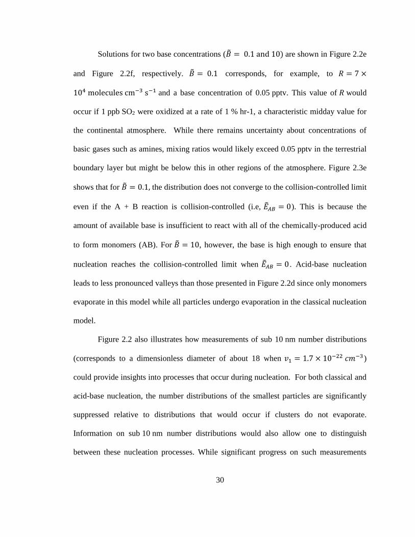
distribution, using the collision-controlled limit as a baseline. Figure 2.2 displays the
sensitivity of dimensionless number distributions to 𝑊, √𝐿, 𝑀, 𝐸 and ��𝐴𝐵 at 𝜏 = 100. To
allow concentrations of discrete sizes and distribution functions to be shown on the same
plot, discrete concentrations were converted to distribution functions using the following
transformation:
𝑑��
𝑑𝑙𝑜𝑔10��𝑝|discrete size 𝑖
= ��
𝑙𝑜𝑔10(𝑖+1
2)1/3
−𝑙𝑜𝑔10(𝑖−1
2)1/3 (2.16)
The minimum size plotted ( ��𝑝 =1.24)) corresponds to the monomer. Wall
deposition (𝑊), scavenging by pre-existing particles (√𝐿) and dilution (𝑀) (Figures 2.2a-
2.2c) have qualitatively similar effects on the distribution: as the rate constants increase,
particle concentrations decrease for all particle sizes with the second peak in the
distribution eliminated. However, for the same value of a rate constant (i.e.,
dimensionless parameter), dilution has a bigger effect than scavenging by preexisting
particles or wall deposition since the impacts of the latter processes decrease with
increasing particle size, while dilution affects all sizes equally. The influence of
evaporation (Figures 2.2d-2.2f) is different in that total particle volume concentrations
are redistributed rather than lost. For both nucleation scenarios, concentrations of 1 <
��𝑝 < 10 particles decrease sharply as the evaporation rate constants increase.
30
Solutions for two base concentrations (�� = 0.1 and 10) are shown in Figure 2.2e
and Figure 2.2f, respectively. �� = 0.1 corresponds, for example, to 𝑅 = 7 ×
104 molecules cm−3 s−1 and a base concentration of 0.05 pptv. This value of 𝑅 would
occur if 1 ppb SO2 were oxidized at a rate of 1 % hr-1, a characteristic midday value for
the continental atmosphere. While there remains uncertainty about concentrations of
basic gases such as amines, mixing ratios would likely exceed 0.05 pptv in the terrestrial
boundary layer but might be below this in other regions of the atmosphere. Figure 2.3e
shows that for �� = 0.1, the distribution does not converge to the collision-controlled limit
even if the A + B reaction is collision-controlled (i.e, ��𝐴𝐵 = 0). This is because the
amount of available base is insufficient to react with all of the chemically-produced acid
to form monomers (AB). For �� = 10, however, the base is high enough to ensure that
nucleation reaches the collision-controlled limit when ��𝐴𝐵 = 0 . Acid-base nucleation
leads to less pronounced valleys than those presented in Figure 2.2d since only monomers
evaporate in this model while all particles undergo evaporation in the classical nucleation
model.
Figure 2.2 also illustrates how measurements of sub 10 nm number distributions
(corresponds to a dimensionless diameter of about 18 when 𝑣1 = 1.7 × 10⁻²² 𝑐𝑚−3)
could provide insights into processes that occur during nucleation. For both classical and
acid-base nucleation, the number distributions of the smallest particles are significantly
suppressed relative to distributions that would occur if clusters do not evaporate.
Information on sub 10 nm number distributions would also allow one to distinguish
between these nucleation processes. While significant progress on such measurements
31
has been made over the past decade, measurement uncertainties need to be reduced to
allow such measurements to reach their full potential.
Figure 2.2. Effects of 𝑊, √𝐿, 𝑀, 𝐸 and ��𝐴𝐵 on dimensionless number distributions at
t =100. Note that results approach the collision-controlled limit for the smallest values of
𝑊, √𝐿, 𝑀, 𝐸 and ��𝐴𝐵 except when �� = 0.1.
2.3.2 Particles Larger Than Cut-off Sizes
32
Aerosol instruments such as CPCs often have cut-off sizes below which detection
efficiencies drop sharply. Therefore, it is sometimes useful to compare the predicted and
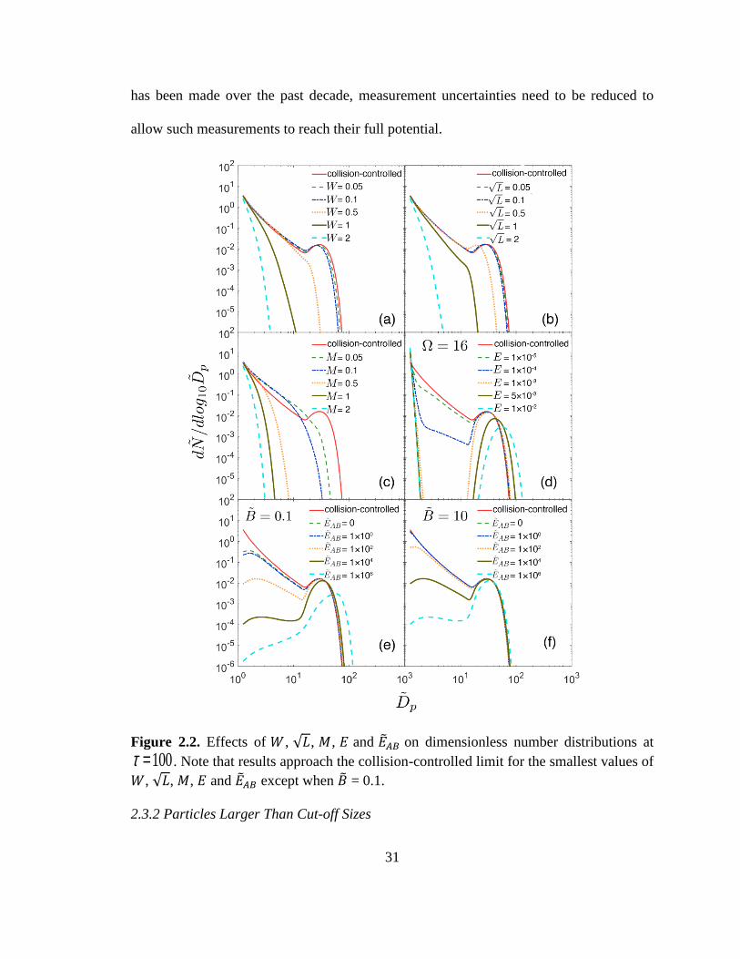
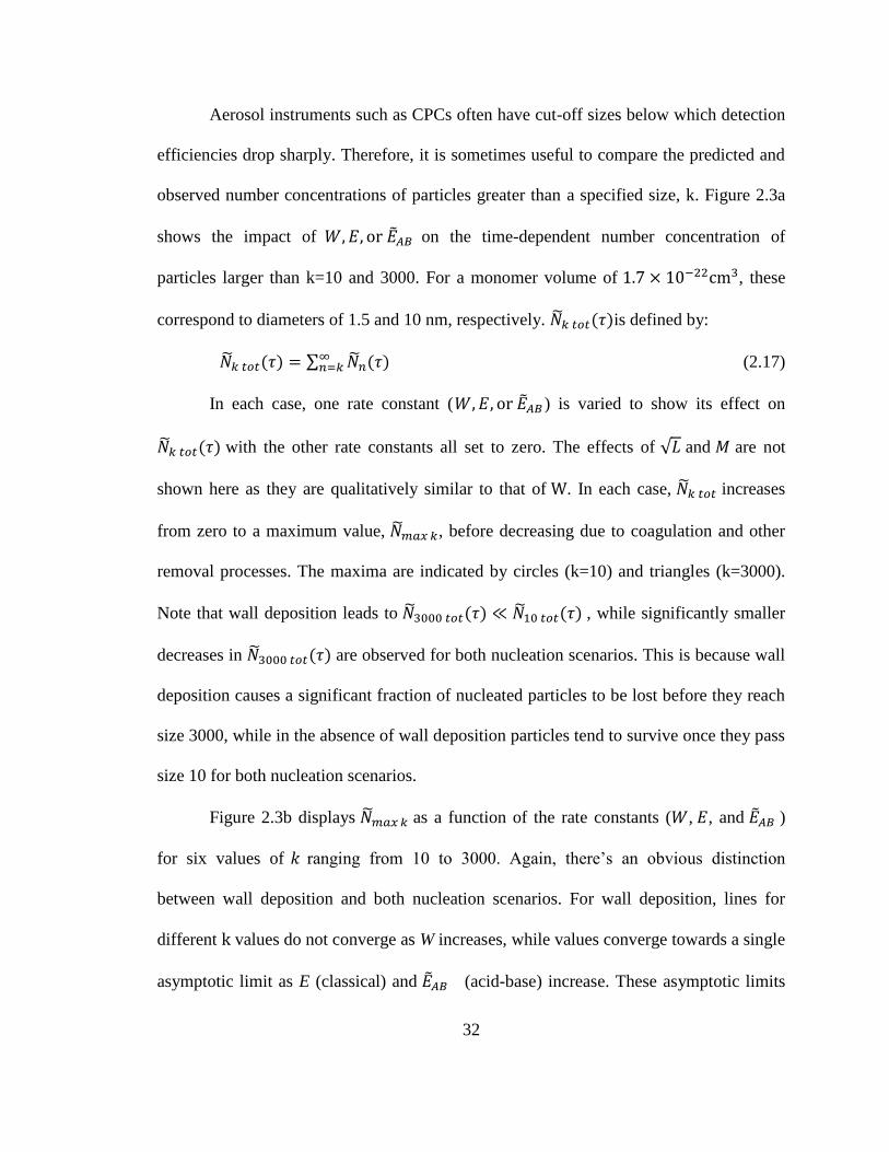
observed number concentrations of particles greater than a specified size, k. Figure 2.3a
shows the impact of 𝑊,𝐸, or ��𝐴𝐵 on the time-dependent number concentration of
particles larger than k=10 and 3000. For a monomer volume of 1.7 × 10⁻²²cm3, these
correspond to diameters of 1.5 and 10 nm, respectively. ��𝑘 𝑡𝑜𝑡(𝜏)is defined by:
��𝑘 𝑡𝑜𝑡(𝜏) = ∑ ��𝑛(𝜏)∞𝑛=𝑘 (2.17)
In each case, one rate constant (𝑊,𝐸, or ��𝐴𝐵 ) is varied to show its effect on
��𝑘 𝑡𝑜𝑡(𝜏) with the other rate constants all set to zero. The effects of √𝐿 and 𝑀 are not
shown here as they are qualitatively similar to that of W. In each case, ��𝑘 𝑡𝑜𝑡 increases
from zero to a maximum value, ��𝑚𝑎𝑥 𝑘, before decreasing due to coagulation and other
removal processes. The maxima are indicated by circles (k=10) and triangles (k=3000).
Note that wall deposition leads to ��3000 𝑡𝑜𝑡(𝜏) ≪ ��10 𝑡𝑜𝑡(𝜏) , while significantly smaller
decreases in ��3000 𝑡𝑜𝑡(𝜏) are observed for both nucleation scenarios. This is because wall
deposition causes a significant fraction of nucleated particles to be lost before they reach
size 3000, while in the absence of wall deposition particles tend to survive once they pass
size 10 for both nucleation scenarios.
Figure 2.3b displays ��𝑚𝑎𝑥𝑘 as a function of the rate constants (𝑊, 𝐸, and ��𝐴𝐵 )
for six values of 𝑘 ranging from 10 to 3000. Again, there’s an obvious distinction
between wall deposition and both nucleation scenarios. For wall deposition, lines for
different k values do not converge as W increases, while values converge towards a single
asymptotic limit as E (classical) and ��𝐴𝐵 (acid-base) increase. These asymptotic limits
33
occur because (i) fewer particles are formed as the evaporation parameters increase,
decreasing the effects of coagulation, and (ii) particles that do form tend to survive.
��𝑘 𝑡𝑜𝑡(𝜏) drops rapidly with W and E, but less rapidly with ��𝐴𝐵 . The more gradual
decrease with ��𝐴𝐵 is due, in part, to the constant base concentration assumed in the model
and the stability of clusters larger than monomer. The model implies that classical
nucleation tends to produce particles in a single burst, while nucleation resulting from
chemical processes (such as acid-base reactions) tends to be more sustained.
Figure 2.3. (a) Effects of 𝑊,𝐸 𝑎𝑛𝑑 ��𝐴𝐵 on and time-dependent total concentrations
��𝑘 𝑡𝑜𝑡(𝜏) for k =10 and 3000, and (b) ��𝑚𝑎𝑥 𝑘 versus 𝑊,𝐸 𝑎𝑛𝑑 ��𝐴𝐵 for several values of
k. Results for L and M are qualitatively similar to those for W and are therefore not
included.
2.3.3 Evolution of Particle Size Distribution
34
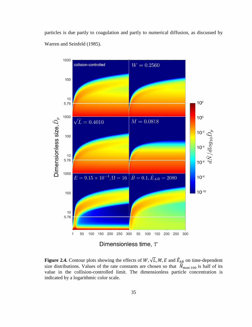
Contour plots can be utilized to conveniently visualize the development of
particle distributions for the entire time span of simulation. Figure 2.4 displays contour
plots of time-dependent number distributions for the collision-controlled limit and for
selected values of 𝑊, √𝐿, 𝑀, 𝐸 & Ω and ��𝐴𝐵 & 𝐵. The particle number distributions are
represented by a logarithmic color scale with red representing the highest concentration
and blue the lowest. Due to the wide range of particle concentration, dimensionless
concentrations lower than 1 × 10⁻¹⁰ are artificially set to 1 × 10⁻¹⁰. Values of the rate
constants are chosen such that ��𝑚𝑎𝑥100 would be half of its value reached in the
collision-controlled limit. The horizontal line at ��𝑝 = 5.76 corresponding to k=100 is
shown for reference.
The contour plots for W and √L are similar to that of the collision-controlled limit
although particle concentrations are somewhat lower for all sizes and the average particle
size is somewhat smaller. In contrast, dilution (𝑀) leads to distributions that reach a
steady state at approximately 𝜏 = 80. 𝑊, √𝐿 and 𝑀 all lead to permanent removal of
particulate mass from the nucleated aerosol, but with different size dependencies. Losses
by wall deposition and scavenging by preexisting particles decrease with increasing size
𝑊 and √𝐿 , while M affects all particle sizes equally and at steady state newly generated
particle volume compensates for sampling losses.
For both nucleation scenarios, new particles are formed in the early stage of the
simulation. These particles serve as condensation sinks and continue to grow and become
more polydisperse as time progresses. Such widening of the distribution for these
35
particles is due partly to coagulation and partly to numerical diffusion, as discussed by
Warren and Seinfeld (1985).
Figure 2.4. Contour plots showing the effects of 𝑊,√𝐿,𝑀, 𝐸 and ��𝐴𝐵 on time-dependent
size distributions. Values of the rate constants are chosen so that ��max100 is half of its
value in the collision-controlled limit. The dimensionless particle concentration is
indicated by a logarithmic color scale.
36
2.4 Conclusions
We used a discrete-sectional model to simulate the dynamic behavior of aerosols
in chemically reacting systems. The population balance equations were cast in a
nondimensional form that reveals the dimensionless parameters that quantify the effects
of various sink processes. Based on our simulations, we draw the following conclusions:
1. The use of the free molecular collision frequency function, rather than the
transition regime expression, is justified for simulations described in this study.
This is because most coagulation occurs among the smallest particles.
2. For every sink process except acid-base nucleation, the collision-controlled limit
is reached provided the corresponding dimensionless rate constant approaches
zero. For acid-base nucleation, the collision-controlled limit is reached only when
the base concentration is sufficiently high.
3. Different sink processes target particles of different sizes. Specifically, dilution
has the same effect on all particle sizes. Evaporation, either in the classical
nucleation model or acid-base nucleation model, preferentially affects the smallest
sizes. Wall deposition and loss to preexisting particles affect particles of all sizes,
although at rates that decrease with increasing size. These size-dependencies
impact the time dependent size distributions that would be observed in a chamber
experiment or the atmosphere.
4. Dimensionless rate constants embody the dependence of sink processes on
material properties and experimental conditions, and are straightforward to
calculate. Care must be taken to avoid errors due to dilution or wall deposition
when calculating monomer formation rates, R.

37
Our analysis leads to dimensionless parameters (Table 2.1) that determine
whether or not a given process significantly affects size distributions of nucleated
particles. When the parameters are sufficiently large, effects become significant. We have
formulated the theory to include all of the processes that were considered, but for
simplicity we have shown numerical results that consider the effects of only an individual
process. In practice, multiple processes are likely to occur simultaneously, and in that
case the equations must be solved to account for their simultaneous effects. For example,
wall deposition and dilution always occur in chamber experiments reported by CLOUD,
and cluster evaporation occurs for some chemical systems. Collectively, these processes
will have a greater effect than any individual process, so deviations from the collision-
controlled limit will occur at smaller values of the dimensionless parameters than are
reported here for individual processes.
38
2.5 Nomenclature
Roman:
𝐴𝐹𝑢𝑐ℎ𝑠 aerosol surface area concentration, corrected to account for transition
regime condensation
= ∫4
3(𝐾𝑛+𝐾𝑛2)
1+1.71𝐾𝑛+4
3𝐾𝑛2
∞
𝑑𝑝 𝑚𝑖𝑛𝜋𝑑𝑝
2𝑛(𝑑𝑝)𝑑𝑑𝑝
where 𝑑𝑝 𝑚𝑖𝑛 is the smallest size of pre-existing particles
[𝐴] concentration of free acid
[��] dimensionless concentration of free acid
[𝐵] concentration of free base
[��] dimensionless concentration of free base
𝛽𝑖𝑗 collision frequency function for clusters that contain i and j monomer
𝛽𝑖𝑗 𝑓𝑚 free molecular expression for i-j collisions
= (3
4𝜋)1/6
(6𝑘𝑏𝑇
𝜌)1/2
𝑣11/6
(1
𝑖+
1
𝑗)1/2
(𝑖1/3 + 𝑗1/3)2
𝑐𝑖𝑗 dimensionless free molecular collision function for i-j clusters
=𝛽𝑖𝑗 𝑓𝑚
𝛽11 𝑓𝑚=
1
4(2)1/2 (1
𝑖+
1
𝑗)1/2
(𝑖1/3 + 𝑗1/3)2
𝑐𝑖𝐴 =𝛽𝑖𝐴 𝑓𝑚
𝛽11 𝑓𝑚=
1
4(2)1/2(1
𝑖+
𝑣1
𝑚𝐴/𝜌𝐴)1/2
(𝑖1/3 + (𝑚𝐴/𝜌𝐴
𝑣1)1/3
)2
𝐶𝑤 Chamber wall loss constant as defined by Kurten et al. (2014)
𝑑𝑝 particle diameter
��𝑝 dimensionless particle diameter
= 𝑑𝑝/𝑣11/3
= (6𝑘/𝜋)1/3 = (6𝑣/(𝜋𝑣1))1/3
39
𝐷𝑠 diffusion coefficient for species s
𝐸𝑗 Monomer evaporation rate constant from size j clusters
= 𝛽11 𝑓𝑚𝑁𝑠𝑎𝑡exp [3
2Ω(𝑗2/3 − (𝑗 − 1)2/3)]
𝑘𝐴+𝐵 forward rate constant for the reaction A+BAB, assumed equal to the A
+ B collision rate
𝐸𝐴𝐵 evaporation rate constant for the reaction ABA+B
𝐾𝐴𝐵 equilibrium constant for A+BAB, =𝑘𝐴+𝐵
𝐸𝐴𝐵
𝑘𝑏 Boltzmann's constant
Kn Knudsen Number , = 2𝜆/𝑑𝑝
𝑚𝑠 mass of species s
n(dp) number distribution function of preexisting aerosol
=𝑑𝑁
𝑑𝑑𝑝, where N is total number concentration
𝑁𝑗 concentration of clusters that contain j monomer
��𝑗 dimensionless concentration of clusters that contain j monomer
𝑁𝑠𝑎𝑡 saturation vapor concentration of condensing monomer
R rate of monomer formation by gas phase reaction
𝑄𝑑𝑖𝑙 volumetric flow rate of particle free air entering a rigid reactor
t time
T absolute temperature
𝑣1 monomer volume = 𝑚1/𝜌
𝑉𝑐ℎ𝑎𝑚𝑏𝑒𝑟 volume of rigid chamber
40
Greek:
𝛿2𝑗 Kronecker delta function (=1 for j=2, and =0 for j2)
𝜆 mean free path
𝜌 particle density
𝜎 surface tension
𝜏 dimensionless time

41
Chapter 3: Errors in Nanoparticle Growth Rates Inferred from
Measurements in Chemically Reacting Aerosol Systems
Abstract: In systems where aerosols are being formed by chemical transformations,
individual particles grow due to the addition of molecular species. Efforts to
improve our understanding of particle growth often focus on attempts to reconcile
observed growth rates with values calculated from models. However, because it is
typically not possible to measure the growth rates of individual particles in
chemically reacting systems, they must be inferred from measurements of aerosol
properties such as size distributions, particle number concentrations, etc. This work
discusses errors in growth rates obtained using methods that are commonly
employed for analyzing atmospheric data. We analyze "data" obtained by
simulating the formation of aerosols in a system where a single chemical species is
formed at a constant rate, R. We show that the maximum overestimation error in
measured growth rates occurs for collision-controlled nucleation in a single-
component system in the absence of a pre-existing aerosol, wall losses, evaporation
or dilution, as this leads to the highest concentrations of nucleated particles. Those
high concentrations lead to high coagulation rates that cause the nucleation mode to
grow faster than would be caused by vapor condensation alone. We also show that
preexisting particles, when coupled with evaporation, can significantly decrease the
concentration of nucleated particles. This can lead to decreased discrepancies
between measured growth rate and true growth rate by reducing coagulation
between nucleated particles. However, as particle sink processes get stronger,
42
measured growth rates can potentially be lower than true particle growth rates. We
briefly discuss nucleation scenarios where the observed growth rate approaches zero
while the true growth rate does not.
3.1 Introduction
Aerosol systems undergo transformations by processes that include coagulation,
convection, deposition on surfaces, source emissions, nucleation, growth, etc. The aerosol
general dynamic equation (GDE) (Friedlander, 2000; Gelbard & Seinfeld, 1979, 1980)
describes the time rate of change of size-dependent particle concentration and
composition by such processes. Recent work has focused on understanding processes
that affect growth rates of freshly nucleated atmospheric nanoparticles (Hodshire et al.,
2016; Kontkanen et al., 2016; Ilona Riipinen et al., 2012; J. Smith et al., 2008; J. N.
Smith et al., 2010; Tröstl et al., 2016).This is important because a particle’s survival
probability increases with growth rates (Kerminen & Kulmala, 2002; C. Kuang, Riipinen,
Yli-Juuti, et al., 2010; P.H. McMurry & Friedlander, 1979; Weber et al., 1997).
Nucleated particles are more likely to form cloud condensation nuclei and affect climate
when survival probabilities are high.
Following established conventions long used in modeling aerosol dynamics
(Friedlander, 2000; Gelbard & Seinfeld, 1979, 1980), we define the particle “growth rate”
as the net rate of change in diameter of individual particles due to the addition or removal
of molecular species. (If evaporation exceeds addition, the growth rate would be
negative.) While most work to date has focused on condensation and evaporation,
chemical processes such as acid-base reactions, organic salt formation, liquid phase
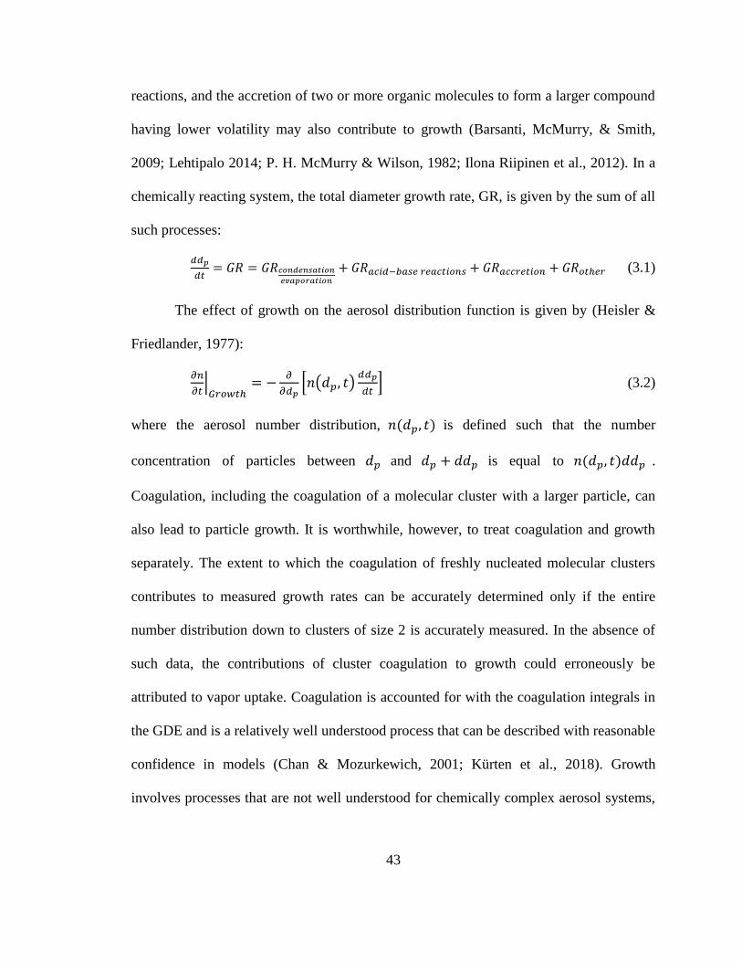
43
reactions, and the accretion of two or more organic molecules to form a larger compound
having lower volatility may also contribute to growth (Barsanti, McMurry, & Smith,
2009; Lehtipalo 2014; P. H. McMurry & Wilson, 1982; Ilona Riipinen et al., 2012). In a
chemically reacting system, the total diameter growth rate, GR, is given by the sum of all
such processes:
𝑑𝑑𝑝
𝑑𝑡= 𝐺𝑅 = 𝐺𝑅𝑐𝑜𝑛𝑑𝑒𝑛𝑠𝑎𝑡𝑖𝑜𝑛
𝑒𝑣𝑎𝑝𝑜𝑟𝑎𝑡𝑖𝑜𝑛
+ 𝐺𝑅𝑎𝑐𝑖𝑑−𝑏𝑎𝑠𝑒 𝑟𝑒𝑎𝑐𝑡𝑖𝑜𝑛𝑠 + 𝐺𝑅𝑎𝑐𝑐𝑟𝑒𝑡𝑖𝑜𝑛 + 𝐺𝑅𝑜𝑡ℎ𝑒𝑟 (3.1)
The effect of growth on the aerosol distribution function is given by (Heisler &
Friedlander, 1977):
𝜕𝑛
𝜕𝑡|𝐺𝑟𝑜𝑤𝑡ℎ
= −𝜕
𝜕𝑑𝑝[𝑛(𝑑𝑝, 𝑡)
𝑑𝑑𝑝
𝑑𝑡] (3.2)
where the aerosol number distribution, 𝑛(𝑑𝑝, 𝑡) is defined such that the number
concentration of particles between 𝑑𝑝 and 𝑑𝑝 + 𝑑𝑑𝑝 is equal to 𝑛(𝑑𝑝, 𝑡)𝑑𝑑𝑝 .
Coagulation, including the coagulation of a molecular cluster with a larger particle, can
also lead to particle growth. It is worthwhile, however, to treat coagulation and growth
separately. The extent to which the coagulation of freshly nucleated molecular clusters
contributes to measured growth rates can be accurately determined only if the entire
number distribution down to clusters of size 2 is accurately measured. In the absence of
such data, the contributions of cluster coagulation to growth could erroneously be
attributed to vapor uptake. Coagulation is accounted for with the coagulation integrals in
the GDE and is a relatively well understood process that can be described with reasonable
confidence in models (Chan & Mozurkewich, 2001; Kürten et al., 2018). Growth
involves processes that are not well understood for chemically complex aerosol systems,
44
such as the atmosphere (Barsanti et al., 2009; Hodshire et al., 2016; Ilona Riipinen et al.,
2012).
Progress towards understanding growth can be achieved through efforts to
reconcile GRs that are observed experimentally with values predicted by models. Such
work requires that size- and time-dependent GRs be accurately determined from
observations. The literature includes many reports of observed GRs (Riccobono, 2012;
Mark R. Stolzenburg et al., 2005; Tröstl et al., 2016; J. Wang, McGraw, & Kuang, 2013),
but uncertainties in reported values are typically not well understood. Because it is
usually not possible to measure the growth of individual particles as they undergo
chemical transformations, GRs are calculated indirectly using time-dependent
observations of aerosol properties such as number distributions or number concentrations
larger than a given size. Those properties are typically affected by many processes, some
poorly understood, that can affect reported GRs to an unknown extent.
A variety of approaches have been used to extract GRs from observations. We
refer to these values as 𝐺𝑅𝑚, where the subscript ‘m’ designates ‘measured’. Methods
that we discuss include:
1. Maximum Concentration Method (Markku Kulmala et al., 2012). During a
nucleation event, particle concentrations in a given size bin increase from their initial
values, passing through a peak before they eventually decrease. This technique involves
noting the times that this maximum occurred in different size bins. The growth rate is
obtained by first fitting a linear function of particle diameter (corresponding to the size
bins) vs. time, and then calculating the slope of the fitted function.

45
2. Appearance Time Method (Lehtipalo 2014). This approach has been used to
analyze data from condensation particle counter (CPC) batteries (Riccobono, 2014),
particle size magnifier (PSM) (Lehtipalo 2014), etc.. In brief, 𝐺𝑅𝑚 is determined by the
differences in concentration rise times (typically, either 5% or 50% of the maximum)
measured by the instruments with differing minimum detection sizes. A variation of this
approach was reported by Weber et al. (1997), who estimated growth rates from the
observed time delay in measurements of sulfuric acid vapor and particles measured with
a condensation particle counter having a minimum detectable size of about 3 nm.
3. Log-normal Distribution Function Method (Markku Kulmala et al., 2012).
Lognormal distributions are fit to the growing mode of nucleated particles. 𝐺𝑅𝑚 is
defined as the growth rate of the geometric mean size of these distributions.
While these methods do not account for the effects of coagulation on measured
changes in particle size, the literature includes approaches that explicitly account for such
effects (C. Kuang et al., 2012; Lehtinen, Rannik, Petaja, Kulmala, & Hari, 2004;
Pichelstorfer et al., 2017; Verheggen & Mozurkewich, 2006). Other work has applied the
above techniques after confirming that coagulation has an insignificant effect for the
analyzed data (Markku Kulmala et al., 2012) or explicitly accounting for the effects of
coagulation on 𝐺𝑅𝑚 (Lehtipalo et al., 2016; Mark R. Stolzenburg et al., 2005).
This chapter assesses errors of using 𝐺𝑅𝑚 calculated using techniques commonly
employed in the literature to infer particle growth rates. Our results are especially
germane to GR of freshly nucleated particles ranging in size from molecular clusters to
about 40 nm. We use time-dependent distribution functions calculated numerically by
McMurry and Li (2017) as “data”. The only process contributing to the addition or
46
removal of molecular species in that work (i.e., to particle “growth rates” as is defined
above) are condensation and evaporation. Because we understand this model system
perfectly, 𝐺𝑅𝑡𝑟𝑢𝑒 (i.e., the net growth rate due molecular exchange through condensation
and evaporation) can be calculated exactly. Errors in 𝐺𝑅𝑚 due to coagulation, wall
deposition, scavenging by preexisting particles, or dilution, are given by the difference
between 𝐺𝑅𝑡𝑟𝑢𝑒 and 𝐺𝑅𝑚. We do not examine errors associated with convection, source
emission, etc.
We are not the first to examine factors that cause 𝐺𝑅𝑚 to differ from 𝐺𝑅𝑡𝑟𝑢𝑒. For
example, Kontkanen (2016) used simulations to show that discrepancies between
measured growth rate based on appearance time (AGR) and growth rate based on
irreversible vapor condensation (CGR) can be significant. (Note 𝐺𝑅𝑡𝑟𝑢𝑒 used in this
chapter differs from CGR in that 𝐺𝑅𝑡𝑟𝑢𝑒 also incorporates evaporation.) Our approach,
which uses the non-dimensional formulation described by McMurry and Li (2017),
provides results that are generally applicable to nucleation and growth of a single
chemical species, so long as it is being produced by chemical transformations at a
constant rate, R. We show that the upper limit for overestimation of 𝐺𝑅𝑡𝑟𝑢𝑒 by 𝐺𝑅𝑚
occurs when nucleation takes place in the absence of pre-existing aerosols and is
collision-controlled (i.e., when evaporation rates from even the smallest clusters occur at
rates that are negligible relative to vapor condensation rates). Collision-controlled
nucleation is an important limiting case because there is growing evidence that
atmospheric nucleation of sulfuric acid with stabilizing species is well-described as a
collision-controlled process (Almeida et al., 2013; Kürten et al., 2018; Peter H. McMurry,
1980). Because cluster evaporation, scavenging by preexisting aerosol, etc., all diminish
47
the number of particles formed by nucleation, overestimation of 𝐺𝑅𝑡𝑟𝑢𝑒 due to
coagulation decreases as these processes gain in prominence. We do not explicitly study
the effect of growth by processes other than condensation or evaporation, such as
heterogeneous growth pathways that take place on or within existing particles. If such
processes were to contribute significantly to growth, they would lead to higher growth
rates and therefore smaller relative errors in 𝐺𝑅𝑚 due to coagulation. Additionally, we
point out when particle sink processes consume nucleated particles at a fast rate (e.g.
strong effects of dilution or scavenging by preexisting particles), 𝐺𝑅𝑚 may not be used to
estimate 𝐺𝑅𝑡𝑟𝑢𝑒. Our results help to inform estimates of uncertainties for systems with a
single condensing species, or systems that can be modeled in a similar way to a single
species system (Kürten et al., 2018).
3.2 Methods
3.2.1 Discrete-sectional Model
We utilize the dimensionless discrete-sectional model described by McMurry and
Li (2017) to simulate evolution of particle size distribution for a system with a single
condensing species. We assume that the condensing species is produced at a constant rate
by gas phase reaction. Our code uses two hundred discrete bins and 250 sectional bins,
with a geometric volume amplification factor of 1.0718 for neighboring sections.
Physical processes that affect particle growth, including wall deposition, loss to
pre-existing particles, cluster evaporation and dilution, can be characterized by
dimensionless parameters in this model. In the present study, however, not all
aforementioned processes are discussed. Our previous work shows that wall losses,
48
scavenging by preexisting particles and dilution have qualitatively similar effects on
aerosol dynamics. Therefore, in this work we focus on preexisting aerosols and dilution
to illustrate factors that contribute to errors in measured growth rates, and do not
explicitly discuss wall deposition. A single dimensionless parameter, √𝐿 , is used to
indicate the abundance of preexisting particles, with larger √𝐿 representing higher
concentration of preexisting particles (or, equivalently, a slower rate at which the
nucleating species is produced by chemical reaction). √𝐿 is calculated with the equation
√𝐿 =
1
4(8𝑘𝑏𝑇
𝜋𝑚1)1/2
𝐴𝐹𝑢𝑐ℎ𝑠
√𝑅𝛽𝑓𝑚 11
(3.3)
where 𝐴𝐹𝑢𝑐ℎ𝑠 is the Fuchs surface area concentration (N. A. Fuchs & A. G. Sutugin,
1971), 𝑘𝑏 is the Boltzmann constant, 𝑚1 is the mass of the monomer, R is the condensing
species production rate, 𝛽11 𝑓𝑚 is the monomer collision frequency function. The loss rate
for particles containing k monomers is √𝐿/𝑘1/2. This size dependence is included when
solving the coupled differential equations for time-dependent cluster concentrations.
Similarly, the dimensionless quantity M that characterizes dilution is given by the
expression
𝑀 =𝑄𝑑𝑖𝑙/𝑉
√𝑅𝛽𝑓𝑚 11
(3.4)
where 𝑄𝑑𝑖𝑙 is the dilution flow rate and V is the volume of the system. Note the fractional
dilution loss is independent of particle size. In addition to loss to pre-existing particles
and dilution, we consider the effect of cluster evaporation on particle growth with the
assumption that evaporation follows the classical liquid droplet model. Two
dimensionless parameters, 𝐸 and 𝛺, are needed to fully describe the evaporation process.

49
The dimensionless evaporation parameter, 𝐸 , is proportional to the saturation vapor
concentration of the nucleating species, while 𝛺 is the dimensionless surface tension
(Peter H. McMurry & Li, 2017; Rao & McMurry, 1989). The evaporation rate for
particles containing k monomers, 𝐸𝑘 , is calculated with a discretized equation of the
form:
𝐸𝑘 = 𝐸𝑐1𝑘 exp [3
2Ω(𝑘
2
3 − (𝑘 − 1)2
3)] (3.5)
where 𝑐(𝑖, 𝑘) is the dimensionless collision frequency between a monomer and a particle
containing k monomers. To simplify our discussion, 𝛺 is fixed to be 16 throughout this
work (a representative value for the surface tension of sulfuric acid aqueous solutions),
while the value of 𝐸 is varied.
The solution to the GDE for a constant rate system (R=constant) depends on
dimensionless time, cluster size and the dimensionless variables √𝐿, M, E, Ω, etc., but is
independent of the rate at which condensing vapor is produced by chemical reaction. That
rate is required to transform the computed nondimensional solutions to dimensional
results using simple multiplicative expressions given by McMurry and Li (2017):
𝑁𝑘 = (𝑅
𝛽11 𝑓𝑚)1/2
��𝑘 ; 𝑡 = (1
𝑅𝛽11 𝑓𝑚)1/2
𝜏 ; 𝑑𝑝 = (𝑣11/3
)��𝑝 (3.6)
In the above equations, ��𝑘 is the dimensionless concentration of particle containing k
monomers, 𝜏 is the dimensionless time, ��𝑝 is the dimensionless particle size and 𝑣1 is
the monomer volume. Assuming a monomer volume of 1.62 × 10⁻²² cm3 (volume of
one sulfuric acid plus one dimethylamine molecule with a density of 1.47 g/cm3), ��𝑝 =
30 would be equivalent to a dimensional particle size of 16.4 nm.
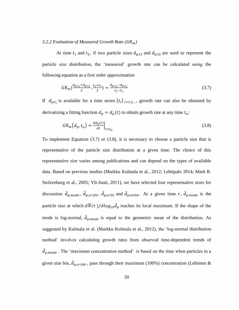
50
3.2.2 Evaluation of Measured Growth Rate (𝐺𝑅𝑚)
At time 𝑡1 and 𝑡2, if two particle sizes 𝑑𝑝,𝑡1 and 𝑑𝑝,𝑡2 are used to represent the
particle size distribution, the ‘measured’ growth rate can be calculated using the
following equation as a first order approximation
𝐺𝑅𝑚(𝑑𝑝,𝑡1+𝑑𝑝,𝑡2
2,𝑡2+𝑡1
2) =
𝑑𝑝,𝑡2−𝑑𝑝,𝑡1
𝑡2−𝑡1 (3.7)
If 𝑑𝑝,𝑡𝑖 is available for a time series {𝑡𝑖} 𝑖=1,2,…, growth rate can also be obtained by
derivatizing a fitting function 𝑑𝑝 = 𝑑𝑝(𝑡) to obtain growth rate at any time 𝑡𝑎:
𝐺𝑅𝑚(𝑑𝑝, 𝑡𝑎) =𝑑𝑑𝑝(𝑡)
𝑑𝑡|𝑡=𝑡𝑎
(3.8)
To implement Equation (3.7) or (3.8), it is necessary to choose a particle size that is
representative of the particle size distribution at a given time. The choice of this
representative size varies among publications and can depend on the types of available
data. Based on previous studies (Markku Kulmala et al., 2012; Lehtipalo 2014; Mark R.
Stolzenburg et al., 2005; Yli-Juuti, 2011), we have selected four representative sizes for
discussion: ��𝑝,𝑚𝑜𝑑𝑒 , ��𝑝,𝑠𝑟100 , ��𝑝,𝑠𝑟50 and ��𝑝,𝑡𝑜𝑡50 . At a given time 𝜏 , ��𝑝,𝑚𝑜𝑑𝑒 is the
particle size at which 𝑑��(τ )/𝑑𝑙𝑜𝑔10��𝑝 reaches its local maximum. If the shape of the
mode is log-normal, ��𝑝,𝑚𝑜𝑑𝑒 is equal to the geometric mean of the distribution. As
suggested by Kulmala et al. (Markku Kulmala et al., 2012), the ‘log-normal distribution
method’ involves calculating growth rates from observed time-dependent trends of
��𝑝,𝑚𝑜𝑑𝑒 . The ‘maximum concentration method’ is based on the time when particles in a
given size bin, ��𝑝,𝑠𝑟100 , pass through their maximum (100%) concentration (Lehtinen &

51
Kulmala, 2003). The ‘appearance time’ method is based on the time when particle
concentrations in a bin, ��𝑝,𝑠𝑟50, pass through a specified percentage of its maximum (we
have used 50%). Growth rates are sometimes based on total concentrations of particles
larger than a specified size. We refer to the particle size above which the total number
concentration of particles reaches 50% of its maximum value as ��𝑝,𝑡𝑜𝑡50. This approach
is especially useful when measurements are carried out with a battery of CPCs having
differing cutoff sizes. For simplicity, in this chapter we assume that CPC detection
efficiencies increase from 0% to 100% at a given cutoff size. In practice, measured size-
dependent detection efficiencies are typically used when analyzing CPC battery data.
Figure 3.1 shows the location of these representative sizes at 𝜏 = 20, 60 ,100 for two
nucleation scenarios in the absence of preexisting particles. ��𝑝,𝑚𝑜𝑑𝑒 , ��𝑝,𝑠𝑟100 , ��𝑝,𝑠𝑟50
and ��𝑝,𝑡𝑜𝑡50 are marked as points, with their y-coordinates representing particle
concentrations at corresponding sizes.
As will be shown later, values of 𝐺𝑅𝑚obtained with ��𝑝,𝑚𝑜𝑑𝑒, ��𝑝,𝑠𝑟100, ��𝑝,𝑠𝑟50 or
��𝑝,𝑡𝑜𝑡50 are not equal. To differentiate these cases, 𝐺𝑅𝑚 are notated as 𝐺𝑅𝑚,𝑚𝑜𝑑𝑒 ,
𝐺𝑅𝑚,𝑠𝑟100, 𝐺𝑅𝑚,𝑠𝑟50 and 𝐺𝑅𝑚,𝑡𝑜𝑡50 accordingly.

52
Figure 3.1. Particle size distributions at dimensionless times 𝜏 = 20, 60 ,100 (a) for
collision-controlled nucleation and (b) when evaporation is included with 𝐸 = 1 × 10⁻³.
Division of the distribution into monomer, cluster and nucleation mode is displayed for
𝜏 = 100, with beige and light blue indicating the range of clusters and nucleation mode.
Clusters and nucleation mode are separated by ��𝑝,𝑚𝑖𝑛, where 𝑑��/𝑑𝑙𝑜𝑔10��𝑝 is at a local
minimum. Characteristic sizes ��𝑝,𝑚𝑜𝑑𝑒, ��𝑝,𝑠𝑟100 , ��𝑝,𝑠𝑟50 and ��𝑝,𝑡𝑜𝑡50 are marked for each
time. The relationship between symbols and characteristic sizes is shown only for =100.
3.2.3 Evaluation of True Growth Rate (𝐺𝑅𝑡𝑟𝑢𝑒)
The true growth rate (𝐺𝑅𝑡𝑟𝑢𝑒) defined in this work follows the Lagrangian
approach (Olenius, Riipinen, Lehtipalo, & Vehkamäki, 2014), i.e. tracking the volume
change of individual particles, and only includes molecular species exchange by
condensation and evaporation. It is calculated with the following expression:
𝐺𝑅𝑡𝑟𝑢𝑒 = 𝑑��𝑝
𝑑𝜏=
2
𝜋��𝑝2
𝑑��
𝑑𝜏=
2
𝜋��𝑝2 ∙
��+𝑐(𝑖,𝑘)��1∙𝑑𝜏−𝐸𝑘∙𝑑𝜏−��
𝑑𝜏=
2(𝑐(𝑖,𝑘)��1−𝐸𝑘)
𝜋��𝑝2 (3.9)
where ��𝑝 is the representative size, ��1 is the concentration of monomers, and 𝐸𝑘 is the
particle evaporation rate given by Equation (3.5).

53
If evaporation is negligible (𝐸 = 0) and ��1 is constant, Equation (3.9) leads to a
higher growth rate for smaller particles, mainly because of the increased monomer
collision frequency relative to particle size (Tröstl et al., 2016). Throughout this work
Equation (3.9) is used to evaluate true particle growth rate. Note 𝐺𝑅𝑡𝑟𝑢𝑒 is calculated
from dimensionless size and time, and is therefore dimensionless. Since we focus on
relative values of true and measured growth rates, our conclusions are unaffected by the
dimensionality of GR. However, dimensionless growth rates can be converted to
dimensional values with Equation (3.6).
3.3 Results and Discussion
3.3.1 Error of Using 𝐺𝑅𝑚,𝑚𝑜𝑑𝑒 as 𝐺𝑅𝑡𝑟𝑢𝑒
As mode diameter (��𝑝,𝑚𝑜𝑑𝑒) is often employed to derive particle growth rate, in
this section we discuss the error of using 𝐺𝑅𝑚,𝑚𝑜𝑑𝑒 as a substitute for 𝐺𝑅𝑡𝑟𝑢𝑒 in the
absence of preexisting particles. The effect of preexisting particles is discussed in Sect.
3.3.
Both condensation and coagulation lead to growth of ��𝑝,𝑚𝑜𝑑𝑒. To understand their
relative importance, we attribute 𝐺𝑅𝑚,𝑚𝑜𝑑𝑒 to three processes: monomer condensation
minus evaporation (𝐺𝑅𝑡𝑟𝑢𝑒), coagulation of the mode with clusters (𝐺𝑅𝑚,𝑐𝑙𝑢𝑠𝑡𝑒𝑟) and self-
coagulation of the mode (𝐺𝑅𝑚,𝑠𝑒𝑙𝑓). The latter two processes are the main causes of the
discrepancy between 𝐺𝑅𝑚,𝑚𝑜𝑑𝑒 and 𝐺𝑅𝑡𝑟𝑢𝑒 . To evaluate 𝐺𝑅𝑚,𝑐𝑙𝑢𝑠𝑡𝑒𝑟 and 𝐺𝑅𝑚,𝑠𝑒𝑙𝑓 , the
range of ‘clusters’ and ‘mode’ are defined as illustrated in Figure 3.1 by the two shaded
regions at 𝜏 = 100 : clusters (beige) and nucleation mode (light blue). Clusters and
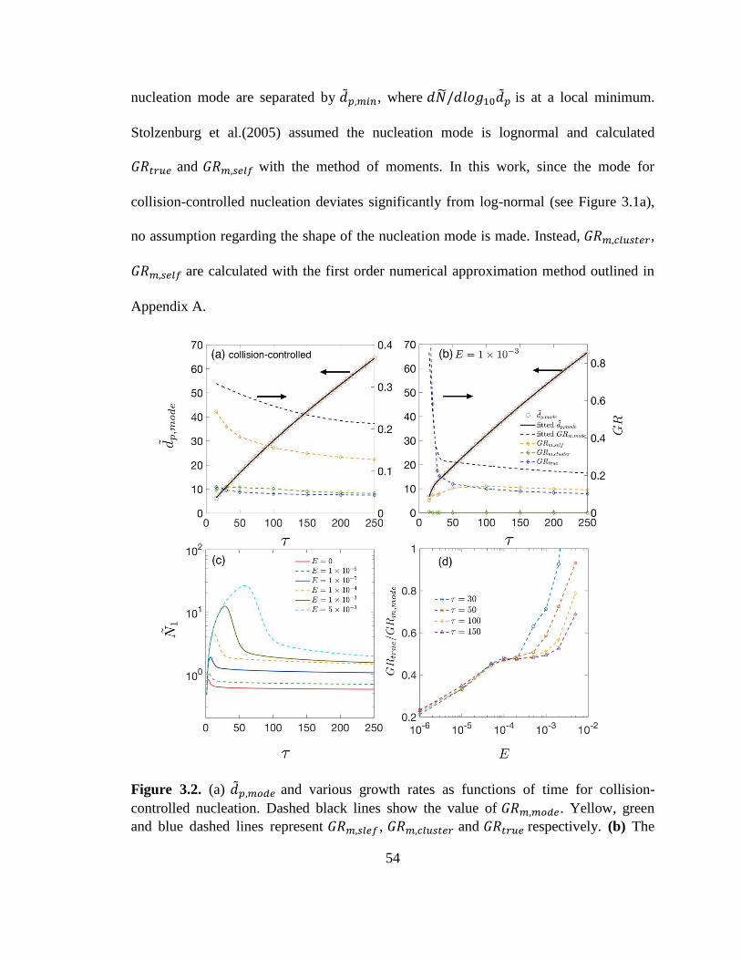
54
nucleation mode are separated by ��𝑝,𝑚𝑖𝑛, where 𝑑��/𝑑𝑙𝑜𝑔10��𝑝 is at a local minimum.
Stolzenburg et al.(2005) assumed the nucleation mode is lognormal and calculated
𝐺𝑅𝑡𝑟𝑢𝑒 and 𝐺𝑅𝑚,𝑠𝑒𝑙𝑓 with the method of moments. In this work, since the mode for
collision-controlled nucleation deviates significantly from log-normal (see Figure 3.1a),
no assumption regarding the shape of the nucleation mode is made. Instead, 𝐺𝑅𝑚,𝑐𝑙𝑢𝑠𝑡𝑒𝑟,
𝐺𝑅𝑚,𝑠𝑒𝑙𝑓 are calculated with the first order numerical approximation method outlined in
Appendix A.
Figure 3.2. (a) ��𝑝,𝑚𝑜𝑑𝑒 and various growth rates as functions of time for collision-
controlled nucleation. Dashed black lines show the value of 𝐺𝑅𝑚,𝑚𝑜𝑑𝑒. Yellow, green
and blue dashed lines represent 𝐺𝑅𝑚,𝑠𝑙𝑒𝑓 , 𝐺𝑅𝑚,𝑐𝑙𝑢𝑠𝑡𝑒𝑟 and 𝐺𝑅𝑡𝑟𝑢𝑒 respectively. (b) The
55
same quantities as are shown in (a) but with the evaporation constant set to 𝐸 = 1 ×10⁻³. For both Figure 3.2a and 3.2b, the left axis shows value for the solid lines and the
right axis shows values for the dashed lines. (c) Monomer concentration as functions of
time for different values of E. (d) 𝐺𝑅𝑡𝑟𝑢𝑒/𝐺𝑅𝑚,𝑚𝑜𝑑𝑒 for different values of 𝐸 at 𝜏 =30, 50, 100, 150.
The calculation results are summarized by Figure 3.2. We first consider collision-
controlled nucleation (E=0). For this nucleation scenario, Figure 3.2a shows ��𝑝,𝑚𝑜𝑑𝑒 on
the left y axis and growth rate values on the right. A third order polynomial is used for
fitting ��𝑝,𝑚𝑜𝑑𝑒 = ��𝑝,𝑚𝑜𝑑𝑒(𝜏) and is plotted as a solid black line. Differentiating the fitted
polynomial with respect to time gives the value of 𝐺𝑅𝑚,𝑚𝑜𝑑𝑒. It is clear that 𝐺𝑅𝑡𝑟𝑢𝑒 only
accounts for a small fraction (17%-20%) of 𝐺𝑅𝑚 and is on par with contribution of
𝐺𝑅𝑚,𝑐𝑙𝑢𝑠𝑡𝑒𝑟 (15%-22%). Self-coagulation is the major contributor (62%-78%) to 𝐺𝑅𝑚 .
Thus, using 𝐺𝑅𝑚,𝑚𝑜𝑑𝑒 as a substitute for 𝐺𝑅𝑡𝑟𝑢𝑒 leads to an overestimation by as much as
a factor about 6. We believe collision-controlled nucleation (E=0) in the absence of other
particle loss mechanisms such as wall deposition (W=0) and scavenging by pre-existing
particles (√𝐿=0) provides an upper limit for overestimation of 𝐺𝑅𝑡𝑟𝑢𝑒 for a constant rate
system (R=constant). This is because these conditions lead to the maximum number of
particles that can be produced by nucleation. High concentrations lead to high
coagulation rates, and it is coagulation that is primarily responsible for errors in 𝐺𝑅𝑚.
Furthermore, as is discussed below, the absence of evaporation and scavenging by
nucleated particles keeps monomer concentrations low relative to values achieved when
E0 (see Figure 3.2a). Low monomer concentrations reduce the value of 𝐺𝑅𝑡𝑟𝑢𝑒, thereby
increasing relative errors in 𝐺𝑅𝑚.
56
Distinctive features of particle growth emerge when cluster evaporation is
included by setting 𝐸 = 1 × 10⁻³. Figure 3.2b shows results for this nucleation scenario.
Most noticeably, particles grow considerably faster at early stages of simulation. This
occurs because evaporation depletes clusters and correspondingly increases monomer
concentration. In the absence of pre-existing particles, monomer concentration
accumulates until the supersaturation is high enough for nucleation to take place (see
Figure 3.2c). The accumulated monomers then rapidly condense on the nucleated
particles, leading to the rapid particle growth shown in Figure 3.2b. To capture this rapid
growth, two third-order polynomials are used to fit ��𝑝,𝑚𝑜𝑑𝑒 values for 𝜏 < 40 and 𝜏 > 35
respectively, with an overlapping region for 35 < 𝜏 < 40. Furthermore, in comparison to
collision-controlled nucleation, contribution of 𝐺𝑅𝑚,𝑐𝑙𝑢𝑠𝑡𝑒𝑟 to 𝐺𝑅𝑚,𝑚𝑜𝑑𝑒 becomes
negligible, due to decreased cluster concentration by evaporation. For 𝜏 > 30, 𝐺𝑅𝑡𝑟𝑢𝑒
accounts for about 40%-55% of 𝐺𝑅𝑚,𝑚𝑜𝑑𝑒 , larger than that of collision-controlled
nucleation; for 𝜏 < 25, 𝐺𝑅𝑡𝑟𝑢𝑒 almost entirely accounts for 𝐺𝑅𝑚,𝑚𝑜𝑑𝑒 and even exceeds
𝐺𝑅𝑚,𝑚𝑜𝑑𝑒 at the very beginning of the nucleation. 𝐺𝑅𝑡𝑟𝑢𝑒 /𝐺𝑅𝑚,𝑚𝑜𝑑𝑒 >1 indicates a
rapidly forming nucleation mode, where freshly nucleated particles enter the mode and
skew the mode distribution toward smaller sizes, slowing down the shift of the mode
peak towards larger values.
Increase of 𝐺𝑅𝑡𝑟𝑢𝑒 / 𝐺𝑅𝑚,𝑚𝑜𝑑𝑒 by evaporation is explained by the elevated
monomer concentration due to particle volatility and the smaller number of particles
formed by nucleation: the former increases 𝐺𝑅𝑡𝑟𝑢𝑒, and the latter decreases 𝐺𝑅𝑚,𝑠𝑒𝑙𝑓 and
𝐺𝑅𝑚,𝑐𝑙𝑢𝑠𝑡𝑒𝑟. Figure 3.2c plots monomer concentration ��1 as a function of time for several
57
values of E. Noticeably, monomer concentration elevates with E since higher cluster
evaporation rates require higher monomer concentrations (i.e., higher supersaturation) to
overcome the energy barrier of nucleation. Once nucleation takes place, high monomer
concentration leads to rapid nanoparticle growth rates.
Figure 3.2d shows 𝐺𝑅𝑡𝑟𝑢𝑒 / 𝐺𝑅𝑚,𝑚𝑜𝑑𝑒 at 𝜏 = 30, 50, 100, 150 for several E
values. At a given time, 𝐺𝑅𝑡𝑟𝑢𝑒 /𝐺𝑅𝑚,𝑚𝑜𝑑𝑒 clearly increases with E: when evaporation
rates are not negligible (i.e., E0), 𝐺𝑅𝑚,𝑚𝑜𝑑𝑒 is closer to 𝐺𝑅𝑡𝑟𝑢𝑒 than occurs when E=0.
Again, this is because the elevated monomer concentrations increase 𝐺𝑅𝑡𝑟𝑢𝑒 and the
lowered concentrations of clusters and nucleated particles decrease 𝐺𝑅𝑚,𝑐𝑙𝑢𝑠𝑡𝑒𝑟 and
𝐺𝑅𝑚,𝑠𝑒𝑙𝑓 . As E approaches 0, the value of 𝐺𝑅𝑡𝑟𝑢𝑒 /𝐺𝑅𝑚,𝑚𝑜𝑑𝑒 converges to that of the
collision-controlled nucleation (~0.2). One data point, corresponding to 𝐸 = 5 × 10⁻³
and 𝜏 = 30, with a value of 1.8, is not shown in Figure 3.2d. It has a value significantly
greater than unity because of the large quantities of nucleated particles entering the mode,
skewing the mode peak toward smaller sizes.
3.3.2 Comparison of Representative Sizes
In this section we examine how observed growth rate depends on the choice of a
representative size. The application of 𝐺𝑅𝑚,𝑚𝑜𝑑𝑒 to deduce 𝐺𝑅𝑡𝑟𝑢𝑒, though convenient
in practice, depends on the existence of a nucleation mode. However, the nucleation
mode is usually not well defined in the early stage of nucleation. In contrast, growth rate
based on other representative sizes (��𝑝,𝑠𝑟50 , ��𝑝,𝑠𝑟100 and ��𝑝,𝑡𝑜𝑡50) are not dependent on
mode formation and are available for all particle sizes. In light of this, 𝐺𝑅𝑚,𝑠𝑟100 ,
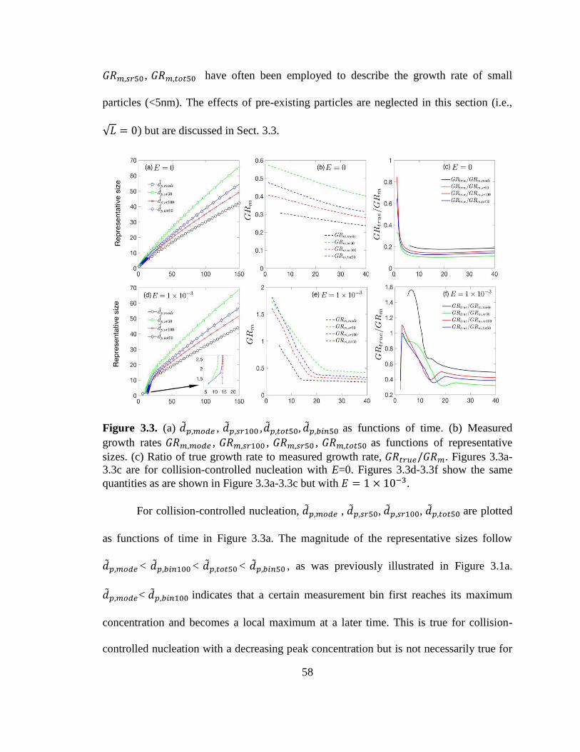
58
𝐺𝑅𝑚,𝑠𝑟50 , 𝐺𝑅𝑚,𝑡𝑜𝑡50 have often been employed to describe the growth rate of small
particles (<5nm). The effects of pre-existing particles are neglected in this section (i.e.,
√𝐿 = 0) but are discussed in Sect. 3.3.
Figure 3.3. (a) ��𝑝,𝑚𝑜𝑑𝑒 , ��𝑝,𝑠𝑟100 ,��𝑝,𝑡𝑜𝑡50, ��𝑝,𝑏𝑖𝑛50 as functions of time. (b) Measured
growth rates 𝐺𝑅𝑚,𝑚𝑜𝑑𝑒 , 𝐺𝑅𝑚,𝑠𝑟100 , 𝐺𝑅𝑚,𝑠𝑟50 , 𝐺𝑅𝑚,𝑡𝑜𝑡50 as functions of representative
sizes. (c) Ratio of true growth rate to measured growth rate, 𝐺𝑅𝑡𝑟𝑢𝑒/𝐺𝑅𝑚. Figures 3.3a-
3.3c are for collision-controlled nucleation with E=0. Figures 3.3d-3.3f show the same
quantities as are shown in Figure 3.3a-3.3c but with 𝐸 = 1 × 10⁻³.
For collision-controlled nucleation, ��𝑝,𝑚𝑜𝑑𝑒 , ��𝑝,𝑠𝑟50, ��𝑝,𝑠𝑟100, ��𝑝,𝑡𝑜𝑡50 are plotted
as functions of time in Figure 3.3a. The magnitude of the representative sizes follow
��𝑝,𝑚𝑜𝑑𝑒 < ��𝑝,𝑏𝑖𝑛100 < ��𝑝,𝑡𝑜𝑡50 < ��𝑝,𝑏𝑖𝑛50 , as was previously illustrated in Figure 3.1a.
��𝑝,𝑚𝑜𝑑𝑒< ��𝑝,𝑏𝑖𝑛100 indicates that a certain measurement bin first reaches its maximum
concentration and becomes a local maximum at a later time. This is true for collision-
controlled nucleation with a decreasing peak concentration but is not necessarily true for
59
other nucleation scenarios. The observed growth rate (i.e. slope of curves in Figure 3.3a)
are shown in Figure 3.3b as a function of representative size, with a clear relationship
𝐺𝑅𝑚,𝑚𝑜𝑑𝑒 < 𝐺𝑅𝑚,𝑠𝑟100 < 𝐺𝑅𝑚,𝑡𝑜𝑡50 < 𝐺𝑅𝑚,𝑠𝑟50. Note that 𝐺𝑅𝑚,𝑚𝑜𝑑𝑒 is not available for
small sizes, indicating the nucleation mode is yet to form at the early stage of nucleation.
Figure 3.3c shows 𝐺𝑅𝑡𝑟𝑢𝑒 / 𝐺𝑅𝑚 as a function of representative size, with 𝐺𝑅𝑡𝑟𝑢𝑒
calculated with Equation (3.9). Clearly 𝐺𝑅𝑡𝑟𝑢𝑒 accounts for the highest percentage of
𝐺𝑅𝑚 at the start of nucleation. This is partly due to higher monomer concentrations (see
red solid curve in Figure 3.2c) and partly due to Equation (3.9) that leads to higher true
growth rate for smaller particles: the addition of a monomer leads to a bigger absolute as
well as fractional diameter growth for small particles.
Figures 3.3d-3.3f are counterparts of Figures 3.3a-3.3c, but with evaporation
constant E set to 1 × 10⁻³. Figure 3.3d show that ��𝑝,𝑠𝑟50 and ��𝑝,𝑡𝑜𝑡50 increase relatively
slowly at the start of the simulation (see the amplified figure at the lower right corner of
Figure 3.3d; for reference, the dimensionless sizes of monomer, dimer and trimer are
1.24, 1.56 and 1.79 respectively). Subsequently, a marked change slope of the ��𝑝 =
��𝑝(𝜏) curve is observed, indicating accelerated particle growth. This reflects that
nucleation occurs with a burst of particle formation following a process of monomer and
cluster accumulation. The slow growth of the smallest clusters is an indication that the
accumulation process is slow due to the strength of the Kelvin effect.
Figure 3.3e shows 𝐺𝑅𝑚 obtained by curve fitting after the nucleation burst and
Figure 3.3f shows the corresponding 𝐺𝑅𝑡𝑟𝑢𝑒 / 𝐺𝑅𝑚 values. Different from collision-
controlled nucleation, there is a sharp rise of 𝐺𝑅𝑡𝑟𝑢𝑒/𝐺𝑅𝑚 value at the start of nucleation.
60
This is due to the sharp decrease of the evaporation term in Equation (3.9), causing the
value of 𝐺𝑅𝑡𝑟𝑢𝑒 to increase sharply. As nucleation progresses, the ratio of 𝐺𝑅𝑡𝑟𝑢𝑒 to
𝐺𝑅𝑚,𝑠𝑟100, 𝐺𝑅𝑚,𝑡𝑜𝑡50 and 𝐺𝑅𝑚,𝑠𝑟50 comes close to 1, with 𝐺𝑅𝑚,𝑚𝑜𝑑𝑒 not yet available.
Eventually, 𝐺𝑅𝑡𝑟𝑢𝑒/𝐺𝑅𝑚 for all representative sizes decreases and fall into the range of
30%-50%, with 𝐺𝑅𝑚,𝑚𝑜𝑑𝑒 giving the best estimate of 𝐺𝑅𝑡𝑟𝑢𝑒. Note the value of 𝐺𝑅𝑡𝑟𝑢𝑒/
𝐺𝑅𝑚,𝑚𝑜𝑑𝑒 significantly exceeds unity for ��𝑝 ∈ [5,11] due to the distortion of the mode
toward smaller sizes by high flux of freshly nucleated particles into the mode.
3.3.3 Effect of Pre-existing Particles
Pre-existing particles act as particle sinks to decrease the intensity of nucleation.
Similarly, in chamber experiments, though loss to pre-existing particles is often
eliminated by using air that is initially particle-free, loss of particles to chamber walls is
inevitable. Since wall loss and loss to preexisting particles have qualitatively similar
effects on nucleation (Peter H. McMurry & Li, 2017), we selectively examine the effect
of preexisting particles on growth rate measurements to qualitatively illustrate the effects
of all of these processes. To probe the initial stage of nucleation, we use ��𝑝,𝑏𝑖𝑛50 as the
basis for our analysis, with a comparison of representative sizes presented at the end of
this section. As to the magnitude of √𝐿, we choose √𝐿 ∈ [0,0.3] based on previous work.
It was shown in Figure 3.2b in McMurry and Li (2017) that as √𝐿 exceeds 0.1, particle
size distributions begin to deviate discernably from the collision-controlled case. In
addition, √𝐿 ≈ 0.2 was observed in the ANARChE field campaign carried out in Atlanta
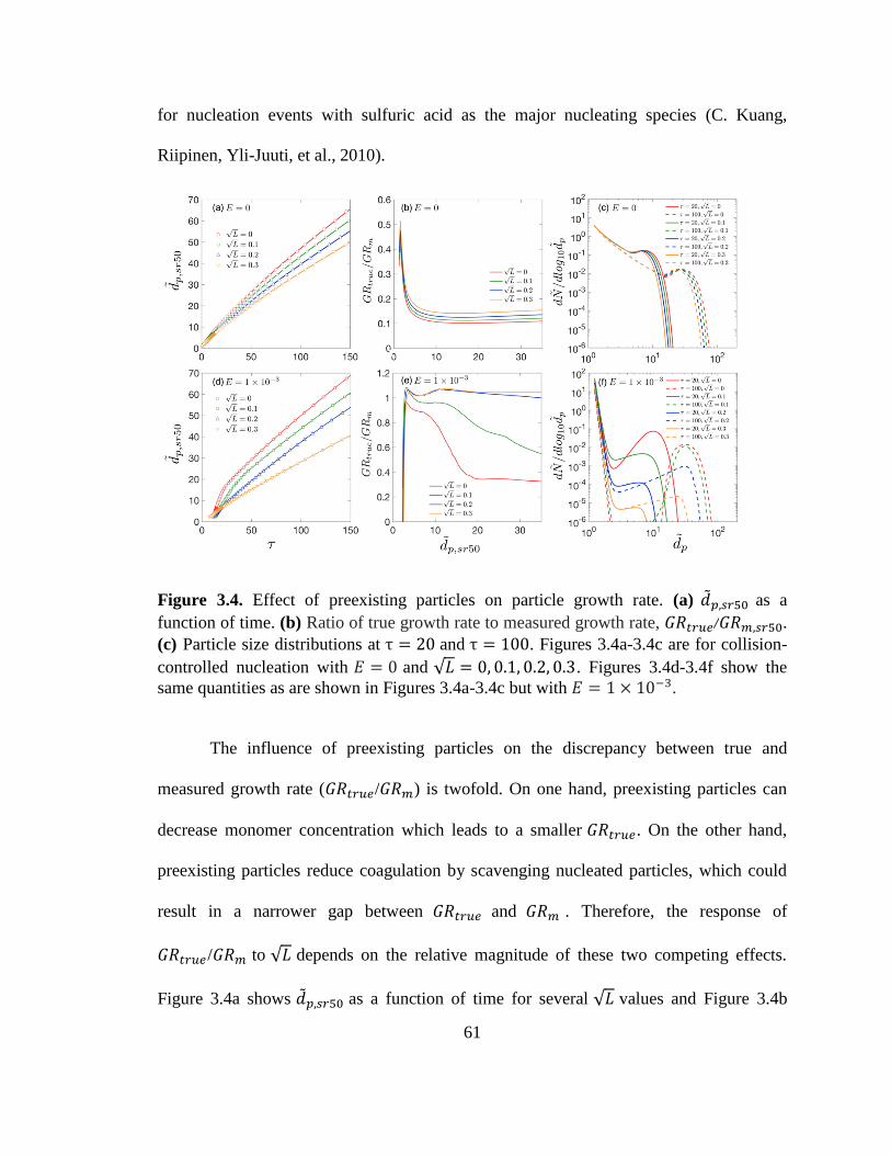
61
for nucleation events with sulfuric acid as the major nucleating species (C. Kuang,
Riipinen, Yli-Juuti, et al., 2010).
Figure 3.4. Effect of preexisting particles on particle growth rate. (a) ��𝑝,𝑠𝑟50 as a
function of time. (b) Ratio of true growth rate to measured growth rate, 𝐺𝑅𝑡𝑟𝑢𝑒/𝐺𝑅𝑚,𝑠𝑟50.
(c) Particle size distributions at τ = 20 and τ = 100. Figures 3.4a-3.4c are for collision-
controlled nucleation with 𝐸 = 0 and √𝐿 = 0, 0.1, 0.2, 0.3. Figures 3.4d-3.4f show the
same quantities as are shown in Figures 3.4a-3.4c but with 𝐸 = 1 × 10⁻³.
The influence of preexisting particles on the discrepancy between true and
measured growth rate (𝐺𝑅𝑡𝑟𝑢𝑒/𝐺𝑅𝑚) is twofold. On one hand, preexisting particles can
decrease monomer concentration which leads to a smaller 𝐺𝑅𝑡𝑟𝑢𝑒. On the other hand,
preexisting particles reduce coagulation by scavenging nucleated particles, which could
result in a narrower gap between 𝐺𝑅𝑡𝑟𝑢𝑒 and 𝐺𝑅𝑚 . Therefore, the response of
𝐺𝑅𝑡𝑟𝑢𝑒/𝐺𝑅𝑚 to √𝐿 depends on the relative magnitude of these two competing effects.
Figure 3.4a shows ��𝑝,𝑠𝑟50 as a function of time for several √𝐿 values and Figure 3.4b
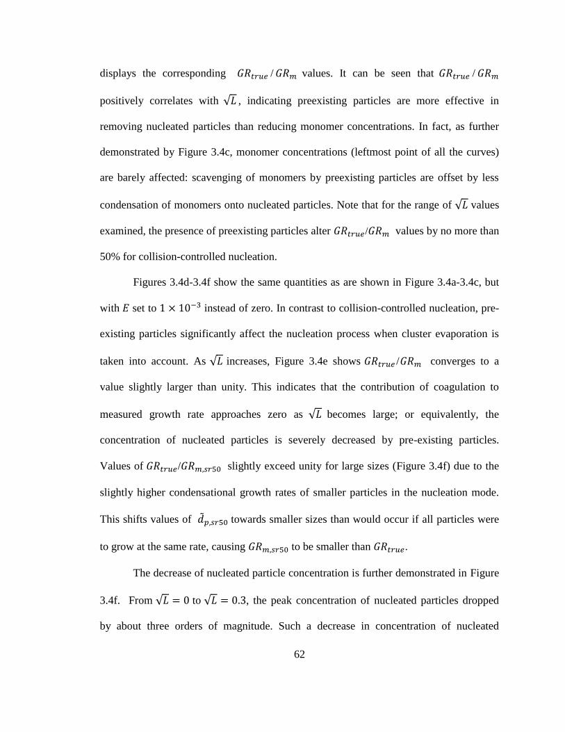
62
displays the corresponding 𝐺𝑅𝑡𝑟𝑢𝑒 / 𝐺𝑅𝑚 values. It can be seen that 𝐺𝑅𝑡𝑟𝑢𝑒 / 𝐺𝑅𝑚
positively correlates with √𝐿 , indicating preexisting particles are more effective in
removing nucleated particles than reducing monomer concentrations. In fact, as further
demonstrated by Figure 3.4c, monomer concentrations (leftmost point of all the curves)
are barely affected: scavenging of monomers by preexisting particles are offset by less
condensation of monomers onto nucleated particles. Note that for the range of √𝐿 values
examined, the presence of preexisting particles alter 𝐺𝑅𝑡𝑟𝑢𝑒/𝐺𝑅𝑚 values by no more than
50% for collision-controlled nucleation.
Figures 3.4d-3.4f show the same quantities as are shown in Figure 3.4a-3.4c, but
with 𝐸 set to 1 × 10⁻³ instead of zero. In contrast to collision-controlled nucleation, pre-
existing particles significantly affect the nucleation process when cluster evaporation is
taken into account. As √𝐿 increases, Figure 3.4e shows 𝐺𝑅𝑡𝑟𝑢𝑒 /𝐺𝑅𝑚 converges to a
value slightly larger than unity. This indicates that the contribution of coagulation to
measured growth rate approaches zero as √𝐿 becomes large; or equivalently, the
concentration of nucleated particles is severely decreased by pre-existing particles.
Values of 𝐺𝑅𝑡𝑟𝑢𝑒/𝐺𝑅𝑚,𝑠𝑟50 slightly exceed unity for large sizes (Figure 3.4f) due to the
slightly higher condensational growth rates of smaller particles in the nucleation mode.
This shifts values of ��𝑝,𝑠𝑟50 towards smaller sizes than would occur if all particles were
to grow at the same rate, causing 𝐺𝑅𝑚,𝑠𝑟50 to be smaller than 𝐺𝑅𝑡𝑟𝑢𝑒.
The decrease of nucleated particle concentration is further demonstrated in Figure
3.4f. From √𝐿 = 0 to √𝐿 = 0.3, the peak concentration of nucleated particles dropped
by about three orders of magnitude. Such a decrease in concentration of nucleated
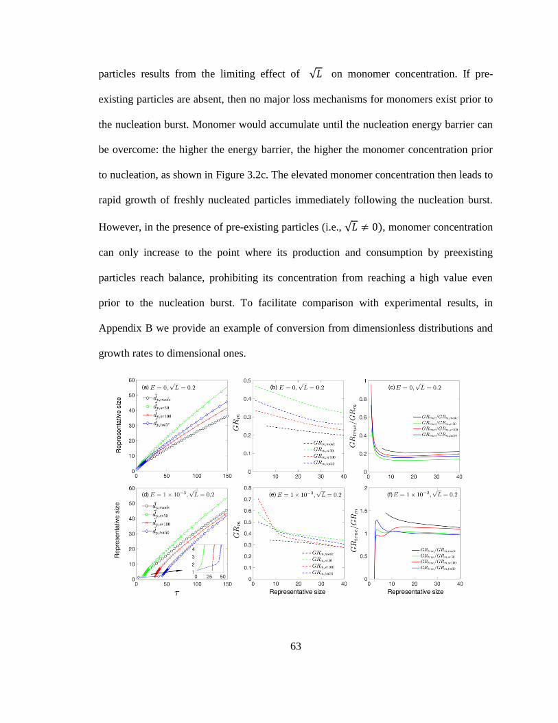
63
particles results from the limiting effect of √𝐿 on monomer concentration. If pre-
existing particles are absent, then no major loss mechanisms for monomers exist prior to
the nucleation burst. Monomer would accumulate until the nucleation energy barrier can
be overcome: the higher the energy barrier, the higher the monomer concentration prior
to nucleation, as shown in Figure 3.2c. The elevated monomer concentration then leads to
rapid growth of freshly nucleated particles immediately following the nucleation burst.
However, in the presence of pre-existing particles (i.e., √𝐿 ≠ 0), monomer concentration
can only increase to the point where its production and consumption by preexisting
particles reach balance, prohibiting its concentration from reaching a high value even
prior to the nucleation burst. To facilitate comparison with experimental results, in
Appendix B we provide an example of conversion from dimensionless distributions and
growth rates to dimensional ones.
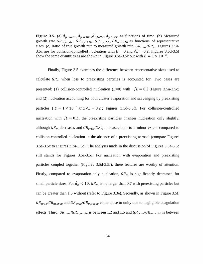
64
Figure 3.5. (a) ��𝑝,𝑚𝑜𝑑𝑒 , ��𝑝,𝑠𝑟100 ,��𝑝,𝑡𝑜𝑡50, ��𝑝,𝑏𝑖𝑛50 as functions of time. (b) Measured
growth rate 𝐺𝑅𝑚,𝑚𝑜𝑑𝑒 , 𝐺𝑅𝑚,𝑠𝑟100 , 𝐺𝑅𝑚,𝑠𝑟50 , 𝐺𝑅𝑚,𝑡𝑜𝑡50 as functions of representative
sizes. (c) Ratio of true growth rate to measured growth rate, 𝐺𝑅𝑡𝑟𝑢𝑒/𝐺𝑅𝑚. Figures 3.5a-
3.5c are for collision-controlled nucleation with 𝐸 = 0 and √𝐿 = 0.2. Figures 3.5d-3.5f
show the same quantities as are shown in Figure 3.5a-3.5c but with 𝐸 = 1 × 10⁻³.
Finally, Figure 3.5 examines the difference between representative sizes used to
calculate 𝐺𝑅𝑚 when loss to preexisting particles is accounted for. Two cases are
presented: (1) collision-controlled nucleation (E=0) with √𝐿 = 0.2 (Figure 3.5a-3.5c)
and (2) nucleation accounting for both cluster evaporation and scavenging by preexisting
particles ( 𝐸 = 1 × 10⁻³ and √𝐿 = 0.2 ; Figures 3.5d-3.5f). For collision-controlled
nucleation with √𝐿 = 0.2 , the preexisting particles changes nucleation only slightly,
although 𝐺𝑅𝑚 decreases and 𝐺𝑅𝑡𝑟𝑢𝑒/𝐺𝑅𝑚 increases both to a minor extent compared to
collision-controlled nucleation in the absence of a preexisting aerosol (compare Figures
3.5a-3.5c to Figures 3.3a-3.3c). The analysis made in the discussion of Figures 3.3a-3.3c
still stands for Figures 3.5a-3.5c. For nucleation with evaporation and preexisting
particles coupled together (Figures 3.5d-3.5f), three features are worthy of attention.
Firstly, compared to evaporation-only nucleation, 𝐺𝑅𝑚 is significantly decreased for
small particle sizes. For ��𝑝 < 10, 𝐺𝑅𝑚 is no larger than 0.7 with preexisting particles but
can be greater than 1.5 without (refer to Figure 3.3e). Secondly, as shown in Figure 3.5f,
𝐺𝑅𝑡𝑟𝑢𝑒/𝐺𝑅𝑚,𝑠𝑟50 and 𝐺𝑅𝑡𝑟𝑢𝑒/𝐺𝑅𝑚,𝑡𝑜𝑡50 come close to unity due to negligible coagulation
effects. Third, 𝐺𝑅𝑡𝑟𝑢𝑒/𝐺𝑅𝑚,𝑚𝑜𝑑𝑒 is between 1.2 and 1.5 and 𝐺𝑅𝑡𝑟𝑢𝑒/𝐺𝑅𝑚,𝑠𝑟100 is between
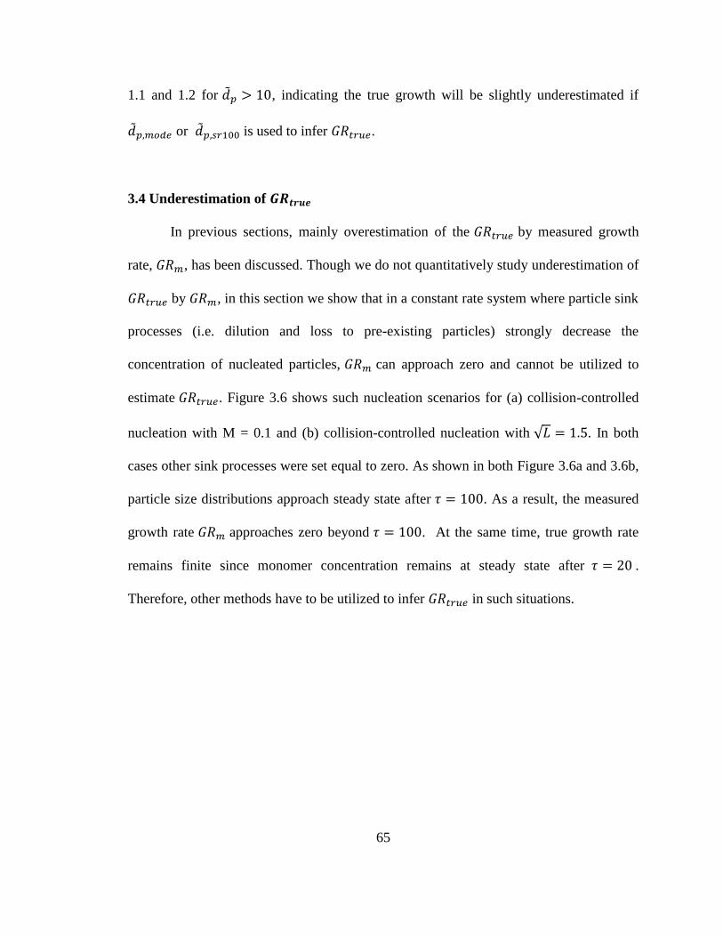
65
1.1 and 1.2 for ��𝑝 > 10, indicating the true growth will be slightly underestimated if
��𝑝,𝑚𝑜𝑑𝑒 or ��𝑝,𝑠𝑟100 is used to infer 𝐺𝑅𝑡𝑟𝑢𝑒.
3.4 Underestimation of 𝑮𝑹𝒕𝒓𝒖𝒆
In previous sections, mainly overestimation of the 𝐺𝑅𝑡𝑟𝑢𝑒 by measured growth
rate, 𝐺𝑅𝑚, has been discussed. Though we do not quantitatively study underestimation of
𝐺𝑅𝑡𝑟𝑢𝑒 by 𝐺𝑅𝑚, in this section we show that in a constant rate system where particle sink
processes (i.e. dilution and loss to pre-existing particles) strongly decrease the
concentration of nucleated particles, 𝐺𝑅𝑚 can approach zero and cannot be utilized to
estimate 𝐺𝑅𝑡𝑟𝑢𝑒. Figure 3.6 shows such nucleation scenarios for (a) collision-controlled
nucleation with M = 0.1 and (b) collision-controlled nucleation with √𝐿 = 1.5. In both
cases other sink processes were set equal to zero. As shown in both Figure 3.6a and 3.6b,
particle size distributions approach steady state after 𝜏 = 100. As a result, the measured
growth rate 𝐺𝑅𝑚 approaches zero beyond 𝜏 = 100. At the same time, true growth rate
remains finite since monomer concentration remains at steady state after 𝜏 = 20 .
Therefore, other methods have to be utilized to infer 𝐺𝑅𝑡𝑟𝑢𝑒 in such situations.
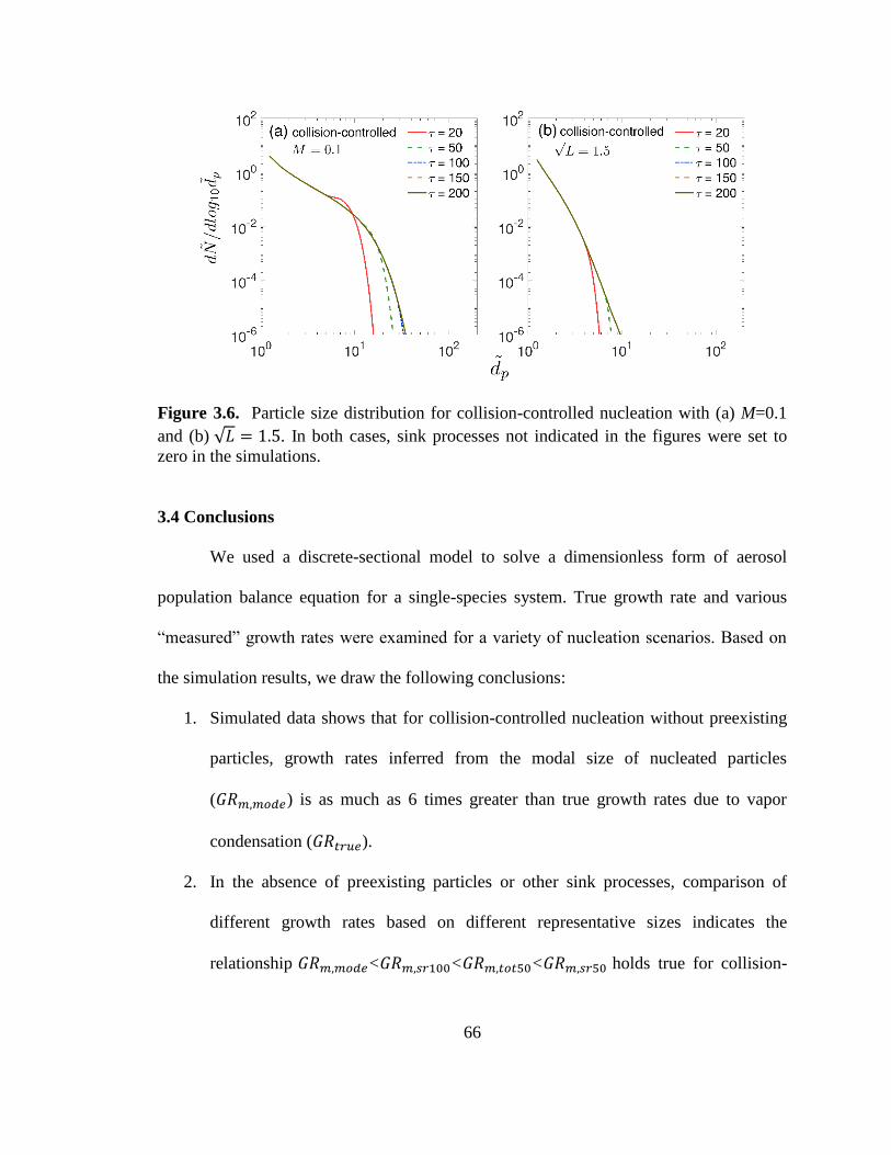
66
Figure 3.6. Particle size distribution for collision-controlled nucleation with (a) M=0.1
and (b) √𝐿 = 1.5. In both cases, sink processes not indicated in the figures were set to
zero in the simulations.
3.4 Conclusions
We used a discrete-sectional model to solve a dimensionless form of aerosol
population balance equation for a single-species system. True growth rate and various
“measured” growth rates were examined for a variety of nucleation scenarios. Based on
the simulation results, we draw the following conclusions:
1. Simulated data shows that for collision-controlled nucleation without preexisting
particles, growth rates inferred from the modal size of nucleated particles
(𝐺𝑅𝑚,𝑚𝑜𝑑𝑒) is as much as 6 times greater than true growth rates due to vapor
condensation (𝐺𝑅𝑡𝑟𝑢𝑒).
2. In the absence of preexisting particles or other sink processes, comparison of
different growth rates based on different representative sizes indicates the
relationship 𝐺𝑅𝑚,𝑚𝑜𝑑𝑒<𝐺𝑅𝑚,𝑠𝑟100<𝐺𝑅𝑚,𝑡𝑜𝑡50<𝐺𝑅𝑚,𝑠𝑟50 holds true for collision-
67
controlled nucleation. If clusters evaporate, the nucleation process is characterized
by rapid particle growth following the nucleation burst.
3. Both evaporation and scavenging by preexisting particles can reduce the
concentration of particles formed by nucleation. Lower particle concentrations
reduce the effect of coagulation on 𝐺𝑅𝑚, so overestimation of 𝐺𝑅𝑡𝑟𝑢𝑒 by 𝐺𝑅𝑚 is
lower than is found in the absence of these processes.
4. Preexisting particles have dramatically different effects on collision-controlled
nucleation and nucleation with cluster evaporation. For √𝐿 ∈ [0,0.3], collision-
controlled nucleation is only slightly affected. However, if preexisting particles
are coupled with evaporation, the number of nucleated particles can drop
significantly, thus reducing the contribution of coagulation to measure growth
rates.
5. 𝐺𝑅𝑚 can underestimate 𝐺𝑅𝑡𝑟𝑢𝑒 in a system with strong dilution or other particle
sink processes. Particle size distributions in such nucleation scenarios can
approach a steady state that leads to a 𝐺𝑅𝑚 close to 0, which underestimates
𝐺𝑅𝑡𝑟𝑢𝑒.
68
Chapter 4: Vapor Specific Extents of Uptake by Nanometer Scale
Charged Particles
Abstract: The uptake of vapor molecules by nanometer scale aerosol particles
(clusters) is of fundamental importance in aerosol science; uptake is the first step of
condensational growth in both the ambient as well as in condensation based particle
detectors. However, uptake is not well understood at the nanometer scale. We
examined the uptake of organic vapor molecules by nanometer scale sodium
chloride cluster ions ((NaCl)x(Na+)z and (NaCl)x(Cl-)z) using a differential mobility
analyzer coupled with a time-of-flight mass spectrometer. Through monitoring
cluster ion inverse mobilities as functions of solvent vapor pressure in the mobility
analyzer, the extent of uptake was monitored for 1-butanol, ethanol, methyl ethyl
ketone (MEK), and toluene. With butanol vapor pressures in the < 300 Pa range,
shifts in inverse mobility excess of a factor of 2 were observed for nearly all
examined clusters. Ethanol and MEK uptake led to shifts for positively charged
cluster ions upwards of a factor of 1.5. Ethanol exposure led to similar sized shifts
for negatively charged clusters ions, while MEK exposure led to negative ion inverse
mobility shifts less than a factor of 1.3. Toluene was sorbed much less efficiently
than the other solvents; toluene exposure led to shifts in inverse mobility below a
factor of 1.2. In total, relative inverse mobility shifts, which are direct functions of
the extent of vapor uptake, were found to be only weakly dependent on cluster ion
size when compared to the influence of vapor molecular structure and cluster ion
charge polarity. Classical (Kelvin-based) models are found inadequate to explain

69
the observed mobility shifts, and we instead used a site-specific, Langmuir type
model to describe the vapor uptake behavior by the cluster ions.
4.1 Introduction
The ability to control vapor uptake by nanoparticles (condensation) with minimal
homogeneous nucleation makes possible the design and operation of condensation
particle counters (CPCs) (P. H. McMurry, 2000). Critically important to CPC
performance is the CPC’s activation efficiency curve, i.e. the fraction of sampled
particles which are condensationally grown to an optically detectable size, as a function
of the original nanoparticle size. Such curves typically take on a value close to unity
above a critical size, but decrease rapidly below it. For > 3 nm particles, the critical size
is determined largely by the Kelvin effect, i.e. the surface tension driven enhancement in
vapor pressure around a small particle. Efforts to decrease the critical size are commonly
made by finding working fluids, aerosol flowrates, and temperature settings for which the
vapor concentration in the CPC growth region exceeds the Kelvin model predicted vapor
pressure at a particle’s surface.
Using the Kelvin model as a guide, commercially available CPCs have been
developed with critical sizes near 3 nm (Iida et al., 2008; M. R. Stolzenburg & McMurry,
1991). Further, recent improvements in CPC design have led to critical sizes in the 1-2
nm mobility size range (Gamero-Castano & Fernandez de la Mora, 2000; Iida et al.,
2009; Chongai Kuang et al., 2012; Vanhanen et al., 2011; Wimmer et al., 2013).
However, in investigating condensation onto 1-2 nm particles, several observations have
been made suggesting that the Kelvin model alone is inappropriate to fully describe the
70
activation efficiency curve for nanometer scale particles. Specifically, dependencies on
particle chemical composition and charge state (i.e. positive or negative) are not expected
based on the Kelvin model (and similarly, the Kelvin-Thomson model). Both particle
chemical composition and charge state have been experimentally observed to have large
effects on CPC activation efficiency in the 1-2 nm range (Iida et al., 2009; Wimmer et al.,
2013), with these effects often difficult to decouple from one another (Kangasluoma,
Samodurov, et al., 2016). The working fluid chemical composition is also observed to
influence activation efficiency in a manner not expected based on the Kelvin model (Iida
et al., 2009).
For 1-2 nm particles, which are composed of a limited number of
atoms/molecules, the main issue with the Kelvin model is presumably that it invokes bulk
matter approximations. In doing so it considers neither effects of molecular scale
interactions between the particle and working fluid molecules, nor the influences of
particle and vapor molecule structure. Molecular interactions and structure govern
completely whether a vapor molecule will bind and remain bound to a surface upon
collision and are particularly important at the nanometer scale. Therefore, in spite of the
continued use of Kelvin model in predicting condensation and growth rates for nanometer
scale species, (M. Kulmala, Kerminen, Anttila, Laaksonen, & O'Dowd, 2004; M.
Kulmala, Lehtinen, & Laaksonen, 2006) there is a clear need to better understand vapor
molecule sorption onto nanometer scale particles.
Recently, our group has shown it is possible to use a differential mobility analyzer
(DMA) coupled to a mass spectrometer (MS) to probe vapor molecule condensation onto
nanometer scale particles (ions) (D. R. Oberreit et al., 2015; Thomas et al., 2016) under
71
sub-saturated conditions. Though CPCs invariably operate under supersaturated
conditions, subsaturated vapor uptake measurements provide information on the earliest
stages of condensation, i.e. they permit examination of the uptake/sorption of several
molecules and importantly, the influences of charge state, particle/ion structure and
working fluid chemical composition. In DMA-MS measurements (or alternative
mobility-mass measurement systems (Rawat, Vidal-de-Miguel, & Hogan, 2015)),
charged species migrating through the mobility classification equilibrate with their
surroundings, which are laden with vapor at a controlled concentrations. As an
ion/particle traverses the mobility classifier vapor molecules sorb and desorb from it; the
net result is a shift in the apparent electrical mobility of the ion/particle from its value in
the absence of vapor. After mobility analysis but prior to mass measurement,
ions/particles pass through a high pressure drop, high electric field interface, in which
nearly all vapor molecules evaporate, and the bare ion/particle is detected in the mass
spectrometer (yielding its chemical composition). Mobility shifts monitored as function
of vapor pressure hence serve to quantify the extent to which a specific vapor sorbs onto
chemically identified ions/particles; these shifts have been shown to be directly linked to
the equilibrium sorption coefficients for successive vapor molecules, as well as the
structures of formed ion/particle-vapor molecule complexes (Oberreit, McMurry, &
Hogan, 2014).
To date, this approach has been applied to proof concept measurements of the
sorption of water vapor to metal halide ions (D. R. Oberreit et al., 2015), to examine
mobility shifts of peptide ions brought about by isopropanol sorption (Rawat et al., 2015),
to examine the influence of vapor sorption on protein ion structure (Meyer, Root, Zenobi,
72
& Vidal-de-Miguel, 2016), and to examine water vapor sorption by dimethylamine-
sulfuric acid clusters (Thomas et al., 2016). In this study, our purpose is to extend such
DMA-MS measurements to examine the sorption of a commonly employed CPC working
fluid (butanol), chemically related compounds, (ethanol, a shorter alcohol than butanol,
and methyl ethyl ketone, MEK, a four carbon compound with a different functional
group), as well as an aromatic compound (toluene) onto positively and negatively
charged sodium chloride clusters/particles of the form (NaCl)x(Na+)z and (NaCl)x(Cl-)z
with x = 1-30 and z = 1-2. In doing so, we demonstrate that the influence of vapor
molecule chemical structure on the earliest stages of condensation is substantial, and is
coupled to the influence of particle charge polarity.
4.2 Experimental Methods
4.2.1 Nanometer Scale Particle/Cluster Generation
Nanometer scale charged species may be interchangeably referred to as cluster
ions or charged particles. For consistency with prior DMA-MS literature, in the
remainder of this work we refer to the species examined as clusters ions. Sodium
chloride cluster ions were generated by electrospray ionization (ESI). The solutions for
ESI were prepared using HPLC grade methanol as solvent with sodium chloride
concentration of 10mM. Both positive and negative ESI were performed following
procedures as described by Hogan and Fernandez de la Mora (Hogan & Fernandez de la
Mora, 2009, 2010), using a silica capillary with an inner diameter of 75µm and outer
diameter of 360µm. For a given experiment, the ESI was operated in stable cone-jet

73
mode and the current carried by produced drops was maintained to be 100-200nA, with a
variation of ±5 nA.
4.2.2 Differential Mobility Analysis-Mass Spectrometry
The DMA-MS system and its operation has been described in detail in previous
studies (Rus et al., 2010). Briefly, singly and multiply charged sodium chloride clusters
ions were directed electrostatically into a parallel plate DMA (SEADM, Boecillo, Spain)
to be separated by electrical mobility. A counter flow of ~0.3 L min-1 was used to prevent
methanol vapor from entering the DMA. A QSTAR XL quadruple time-of-flight mass
spectrometer (qTOF–MS, MDS Sciex) was interfaced with the DMA to determine the
mass-to-charge ratio of the selected ions. The DMA was operated with a circulating
sheath flow pumped by a vacuum blower. DMA calibration was performed for all
experiments by measuring the voltage required to transmit the tetraheptylammonium+ ion
(produced via ESI of tetraheptylammonium bromide dissolved in methanol), as is
commonly used in high sheath flowrate DMA calibration.(Kangasluoma, Attoui, et al.,
2016; Ude & Fernandez de la Mora, 2005) To collect mobility spectra, the voltage
difference across the DMA electrodes was stepped in 10 V increments in the 800-5000 V
range. The temperature of the DMA sheath flow was controlled by a water jacket heat
exchanger at 293±0.5K for all experiments. At each DMA voltage difference, a mass
spectrum in 10-3000 Th range was collected using the time-of-flight section of the
QSTAR XL mass spectrometer. Inlet declustering potentials and focusing potentials,
which aid in particle/ion transmission into the mass spectrometer but also promote
74
fragmentation, were set to minimum values, following Thomas et al (Thomas et al.,
2016).
The DMA sheath flow consisted of high purity N2 with an organic vapor (butanol,
MEK etc.) concentration in the 0.0% to 0.5% range (0-500 Pa). The organic vapor was
added into the sheath flow utilizing a nebulizer as described by Oberreit et al. (2014). A
carrier gas flow (N2) through the nebulizer was maintained at ~0.8 L min-1 during all
experiments. To ensure the nebulized liquids evaporate completely prior to entering the
DMA, the nebulizer was heated to 75˚C with a heating tape. The organic vapor pressure
within the DMA was calculated from the organic liquid flow rate (set using a syringe
pump) and the carrier gas flow rate. Prior to each measurement, the DMA-MS system
(with the sheath flow pump turned on as well as the heat exchanger) was allowed to
equilibrate for 1.5-2 hours. In cases where the sorption of vapor changes the electrical
mobility significantly, constant organic vapor pressure could be ascertained by observing
constant mobilities for a given species over several consecutive measurements.
During DMA-MS measurements, system contamination, even at the parts-per-
million level, can influence measurements (Maisser, Thomas, Larriba-Andaluz, He, &
Hogan, 2015). Contamination at such levels can arise if impurities are present in the
nebulized solvents, which deposit in sheath flow tubing. More concerning is residual
solvent from one experiment carrying over to subsequent experiments. Therefore, prior
to changing solvents, the DMA plates were thoroughly cleaned by disassembling the
DMA and the DMA sheath flow was operated in open loop for hours (days in some
cases) without any solvent introduction. To ensure solvent carryover was mitigated, the
electrical mobilities of sodium chloride cluster ions were measured in dry N2 and were

75
normalized by the electrical mobility of the tetraheptylammonium+ ion. Cleaning was
repeated until the normalized electrical motilities for each singly charged sodium chloride
particle was within 5% of an established baseline value.
4.3 Results and Discussion
4.3.1 Characteristic DMA-MS Mass-Mobility Spectra
Figure 4.1 displays contour plots of the mass-mobility spectra for positively
charged sodium chloride cluster ions ((NaCl)x(Na+)z). Specifically, Figure 4.1a displays
results obtained in the absence of vapor and Figure 4.1b displays results obtained with
butanol introduced into the DMA with a vapor pressure of 166 Pa. Following prior
DMA-MS studies (Ouyang, Larriba-Andaluz, Oberreit, & Hogan, 2013), on the
horizontal axes of contour plots are the inverse mobilities of the cluster ions, while on the
vertical axes are x/z values, where x is the number of neutral ion-pairs (NaCl) in the
cluster ions and z is number of charges the ions possess. Detected signals for the cluster
ions are represented by line segments in the contour plots, with their length defined by
the DMA resolution. Signal intensities are indicated by a logarithmic color scale, with
yellow indicating the lowest intensity above a set threshold and blue the highest. Because
chlorine has two stable isotopes with masses of 35 Da and 37 Da, detection of larger
clusters leads to a series of line segments closely spaced in x/z; these lines are not
discernable from one another in contour plots. Singly charged cluster ions appear near
integer x/z values only, doubly charged ions differ in x/z from another by approximately
½, and higher charge state by 1/z. As is common for electrospray generated clusters
ions,(Hogan & Fernandez de la Mora, 2009) for sodium chloride ions under all
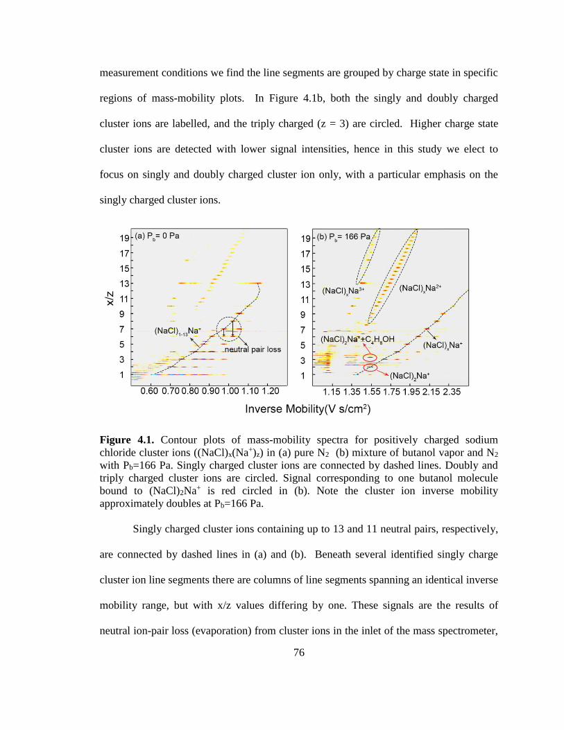
76
measurement conditions we find the line segments are grouped by charge state in specific
regions of mass-mobility plots. In Figure 4.1b, both the singly and doubly charged
cluster ions are labelled, and the triply charged (z = 3) are circled. Higher charge state
cluster ions are detected with lower signal intensities, hence in this study we elect to
focus on singly and doubly charged cluster ion only, with a particular emphasis on the
singly charged cluster ions.
Figure 4.1. Contour plots of mass-mobility spectra for positively charged sodium
chloride cluster ions ((NaCl)x(Na+)z) in (a) pure N2 (b) mixture of butanol vapor and N2
with Pb=166 Pa. Singly charged cluster ions are connected by dashed lines. Doubly and
triply charged cluster ions are circled. Signal corresponding to one butanol molecule
bound to (NaCl)2Na+ is red circled in (b). Note the cluster ion inverse mobility
approximately doubles at Pb=166 Pa.
Singly charged cluster ions containing up to 13 and 11 neutral pairs, respectively,
are connected by dashed lines in (a) and (b). Beneath several identified singly charge
cluster ion line segments there are columns of line segments spanning an identical inverse
mobility range, but with x/z values differing by one. These signals are the results of
neutral ion-pair loss (evaporation) from cluster ions in the inlet of the mass spectrometer,
77
prior to mass measurement ((NaCl)xNa+→(NaCl)x-yNa+ + (NaCl)y) (Hogan & Fernandez
de la Mora, 2010; Ouyang et al., 2013; Trimpin & Clemmer, 2008). Other paths of
dissociation, which could occur either within the DMA or the mass spectrometer inlet are
documented in Ouyang et al (2013) and Thomas et al (Thomas et al., 2016).
Also apparent in contour plots is that the inverse mobilities of singly charged
cluster ions are approximately twice as large when measured with a butanol vapor
pressure (Pb) of 166 Pa in comparison to dry conditions. This is a significantly larger
inverse mobility shift than been observed for nanometer scale ions exposed to water
vapor and isopropanol in prior studies (D. R. Oberreit et al., 2015; Rawat et al., 2015;
Thomas et al., 2016), and suggests that multiple butanol molecules (on average) are
sorbed to the cluster ions in the DMA. These molecules dissociate from cluster ions due
collision activation in the mass spectrometer inlet, prior to mass analysis, (D. R. Oberreit
et al., 2015) as the measured masses of most cluster ions do not shift in the presence of
vapor. However, for the smallest cluster ions (x = 1 or 2), signal is detected for some
ions at a mass-to-charge ratio 74 Th above the baseline mass-to-charge ratio; this
corresponds to the attachment of a single butanol molecule during mass measurement.
Such a mass shift provides direct evidence of butanol sorption, in addition to the indirect
evidence provided by inverse mobility shifts.
Similar to Figure 4.1, Figure 4.2 displays contour plots for negatively charged
cluster ions at Pb = 0 Pa, 44 Pa, 66 Pa and 166 Pa. As was the case for positively charged
ions, significant vapor uptake appears to take place, and the clusters ions have greatly
reduced mobilities (larger inverse mobilities) in the presence of butanol. Positively and
negatively charged cluster ion contour plots are qualitatively similar to one another, with
78
line segments results from neutral loss between mobility and mass measurement present.
However, the contour plots of negative cluster ions have two noteworthy features which
are distinct from the positive case. First, for positively charged cluster ions with z =1,
with the exception of the x = 13 cluster ion (a 3 × 3 × 3 cube (Dugourd, Hudgins, &
Jarrold, 1997)), x/z increases monotonically with inverse mobility. Made apparent by the
dashed guideline in Figure 4.2a this correlation is clearly perturbed for negatively
charged cluster ions; the cluster ions x = 3 and x = 4 have similar inverse mobilities in
the absence of vapor, as do the clusters with x = 7-9. Second, we note that for positively
charged ions, cluster ions of higher mass have higher inverse mobilities than lower mass
clusters for all examined vapor pressures (again with the exception of x = 13). This is not
the case for the x = 2-4 as well as for the x = 7- 9 negatively charged ions exposed to
both butanol and ethanol; for these ion groups the ions which have the largest and
smallest inverse mobilities change with changing vapor pressure. To illustrate this, line
segments corresponding to (NaCl)7Cl-, (NaCl)8Cl-, and (NaCl)9Cl- are circled in all four
Figure 4.2 contour plots. In the absence of vapor, these cluster ions are closely packed
horizontally with inverse mobility values 1
𝑍9>
1
𝑍8>
1
𝑍7 (Zx is the electrical mobility of the
cluster ion containing x neutral pairs). As Pb is increased from 0 to 44 Pa, these clusters
become separated in mobility, with their relative inverse mobility ranking reserved to
1
𝑍7>
1
𝑍8>
1
𝑍9 (i.e. the least massive cluster ion has the largest inverse mobility under this
condition). The relative positions of these cluster ions continue to evolve as Pb increases,
returning to 1
𝑍9>
1
𝑍8>
1
𝑍7 in Figure 4.2d, and remaining as such as Pb is increased
further. A phenomenon similar to this is observed for the (NaCl)2Cl-, (NaCl)3Cl- and
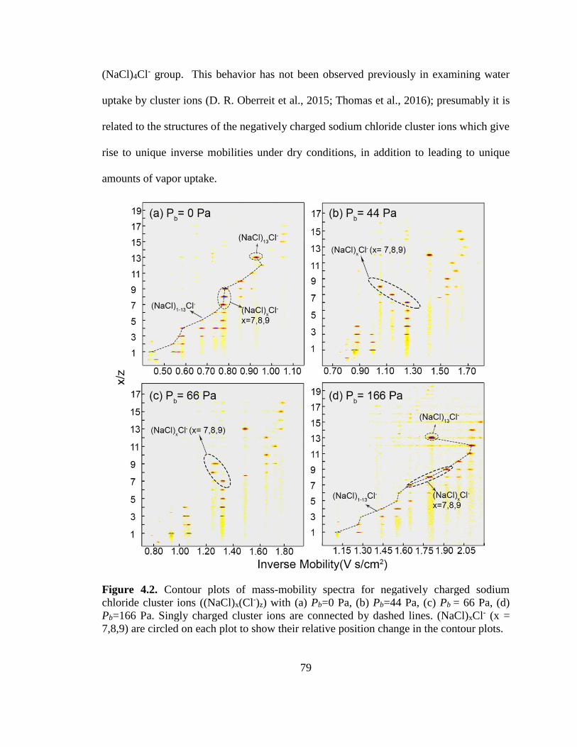
79
(NaCl)4Cl- group. This behavior has not been observed previously in examining water
uptake by cluster ions (D. R. Oberreit et al., 2015; Thomas et al., 2016); presumably it is
related to the structures of the negatively charged sodium chloride cluster ions which give
rise to unique inverse mobilities under dry conditions, in addition to leading to unique
amounts of vapor uptake.
Figure 4.2. Contour plots of mass-mobility spectra for negatively charged sodium
chloride cluster ions ((NaCl)x(Cl-)z) with (a) Pb=0 Pa, (b) Pb=44 Pa, (c) Pb = 66 Pa, (d)
Pb=166 Pa. Singly charged cluster ions are connected by dashed lines. (NaCl)xCl- (x =
7,8,9) are circled on each plot to show their relative position change in the contour plots.
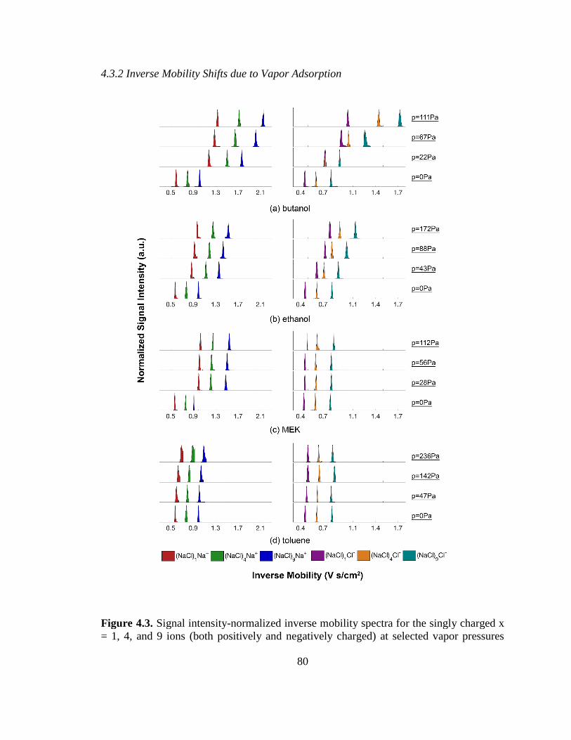
80
4.3.2 Inverse Mobility Shifts due to Vapor Adsorption
Figure 4.3. Signal intensity-normalized inverse mobility spectra for the singly charged x
= 1, 4, and 9 ions (both positively and negatively charged) at selected vapor pressures

81
within the sheath flow. Results are provided for (a) butanol, (b) ethanol, (c) MEK, and
(d) toluene.
It is difficult to explicitly show how the inverse mobility of a particular ion (i.e.
an ion of specific x and z) evolves with changing vapor pressure through contour plots
alone. We therefore elect to display signal intensity-normalized inverse mobility spectra
for the singly charged x = 1, 4, and 9 ions (both positively and negatively charged) at
selected vapor pressures in Figure 4.3. Results are provided with (a) butanol, (b) ethanol,
(c) MEK, and (d) Toluene. These ions were selected because they are found in higher
signal intensity in all measurements (i.e. they were the most easily detected ions).
However, similar conclusions to those presented here would result from examination of
other singly charged cluster ions. Signals resulting from neutral and ion evaporation
events have been removed from Figure 4.3 spectra, hence each peak corresponds to one
of the ions of interest. We display results for each vapor type in a similar vapor pressure
range; though the tested vapors have disparate saturation vapor pressures we find that
𝑑(1
𝑍𝑥)
𝑑𝑃|
𝑇
, the change in inverse mobility per unit change in vapor pressure (at constant
temperature), attains a local maximum in in 0 – 200 Pa vapor pressure range. We remark
that this observation may simply be coincidence for the vapor examined as is by no
means universal for all ion and vapor molecule compositions.
For all tested vapor types, shifts to larger inverse mobilities are apparent, but the
extent of shift is clearly vapor molecule type and charge state specific. Specifically, large
shifts in inverse mobility for ions (larger than a factor of 1.3 when compared to the dry
inverse mobility) are experimentally observed for butanol and ethanol with all singly
charged ions (with significantly larger shifts observed for butanol), as well for the
82
positively charged cluster ions exposed to MEK. Conversely, toluene gives rise to
smaller mobility shifts for all ions, as does MEK for negatively charged cluster ions.
These findings are neither quantitatively nor qualitatively consistent with classical model
predictions considering the Kelvin and Thomson influence alone (all vapor molecules
have similar surface tensions), the influence sodium chloride dissolution may have on
uptake (NaCl is more soluble in ethanol than in butanol), as well as with modifications
classical theory (Yu, 2005) considering ion-dipole and ion-induced dipole interactions
(MEK has the highest dipole moment of any test vapor molecule, while Toluene has the
highest polarizability). While toluene is chemically very distinct from the other test
vapors and differences between them are hence anticipated, the other test vapor
molecules are chemically related; butanol and ethanol share the same functional group
and differ only in carbon chain length, while butanol and MEK share the same number
carbons and differ only in functional group. The variable extents of uptake observed for
these vapor molecules hence suggest that the earliest stages of heterogeneous
condensation onto nanometer scale species are extremely dependent on cluster-vapor
molecule interactions, and small changes to vapor molecule chemical structure or ion
charge state may have drastic influences on the extent of vapor molecule sorption.
4.3.3 Influence of Charge State
Because of the observed deviations in uptake behavior from what is anticipated
based on classical theory, it is of interest to examine the influence of charge state and
cluster size on vapor uptake isolated from another. Figure 4.4 displays the variation in
inverse mobility for selected cluster ions (x = 1, 4, 9, 13) with butanol, ethanol and MEK
83
partial pressure, both positively and negatively charged. Specifically, normalized inverse
mobility, 1
𝑍𝑥|𝑃/
1
𝑍𝑥|0the ratio of the inverse cluster ion mobility at partial pressure p and
to the dry inverse mobility, is plotted as a function of solvent partial pressure. For the
positively charged cluster ions, all the curves are concave downward. The curves
obtained for ethanol sorption are the least concave, butanol curves are intermediate, and
MEK curves display the greatest concavity, as 𝑑(
1𝑍𝑥
)
𝑑𝑃|
𝑇
approaches 0 as MEK partial
pressure increases. Concave inverse mobility versus concentration curves have been
observed previously for isopropanol sorption onto peptide ions (Rawat et al., 2015), and
are also observed when applying mobility to examine protein binding to nanoparticles
(Seongho Jeon et al., 2016; Jeon, Oberreit, Van Schooneveld, & Hogan, 2016). In these
prior studies, this finding has been interpreted as resulting from the binding of molecules
at specific surface site or the formation of a monolayer onto ions/particles. In a
subsequent section, we hence compare the positive cluster ion inverse mobility versus
partial pressure curves to theoretical models of site specific-binding.
Inverse mobility versus partial pressure curves for negative ions have clear
differences from the positive ion curves. The curves describing butanol and ethanol
sorption by negatively charged cluster ions intersect with one another, reflecting the
relative position change of the signal line segments noted previously (Figure 4.2). In the
case of butanol sorption, for negative ions the value of 𝑑(
1𝑍𝑥
)
𝑑𝑃|
𝑇
is larger than for positive
ions at higher partial pressures (i.e. negative ion curves are less concave). Most
prominently, negative cluster ions show minimal uptake of MEK, in stark contrast to
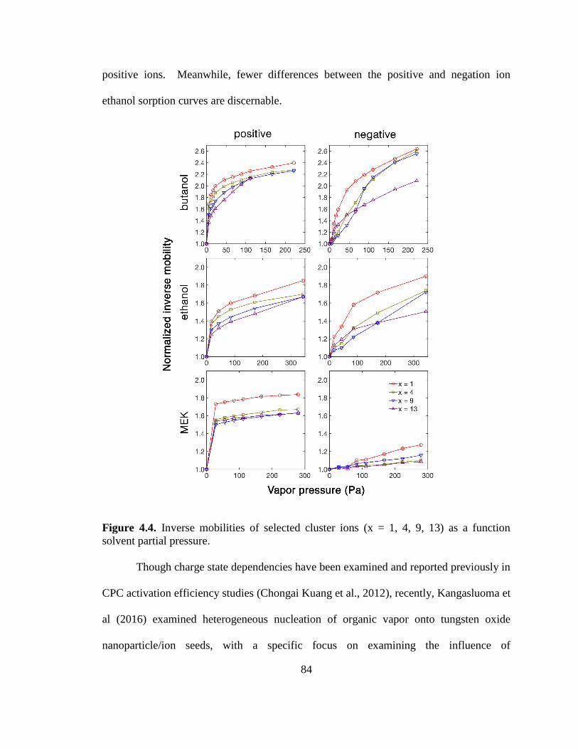
84
positive ions. Meanwhile, fewer differences between the positive and negation ion
ethanol sorption curves are discernable.
Figure 4.4. Inverse mobilities of selected cluster ions (x = 1, 4, 9, 13) as a function
solvent partial pressure.
Though charge state dependencies have been examined and reported previously in
CPC activation efficiency studies (Chongai Kuang et al., 2012), recently, Kangasluoma et
al (2016) examined heterogeneous nucleation of organic vapor onto tungsten oxide
nanoparticle/ion seeds, with a specific focus on examining the influence of

85
nanoparticle/ion charge polarity on the growth process. They suggest that ion charge
state is a less important factor in controlling vapor uptake and growth than is the
chemical composition of the ions; specifically, they found that positive and negative
tungsten oxide ions contained different impurities and that the impurity content had a
larger influence on uptake than the charge polarity. We remark that here the ions of
interest were chemically identified, contained no impurities, and those of different charge
polarity had near identical composition (i.e. positive and negative cluster ions simply
have an Na+ and Cl- exchanged). Therefore, the differences we observe for different
charge state ions cannot be attributed to chemical impurities in ions of different charge
state. In total, our comparison of uptake by ions differing in charge state shows that the
influence of charge polarity is significant and clearly vapor dependent.
4.3.4 Influence of Cluster Size
Figure 4.5 displays plots of the normalized inverse mobility versus solvent partial
pressure curves for (NaCl)xNa+ (x = 1, 4, 9 ,13) clusters (Figure 4.5a) and for
(NaCl)x(Na+)2 (x= 21, 27, 31, 34) (Figure 4.5b). For all the cluster ions displayed,
sorption of butanol molecules produces the most significant inverse mobility shifts and
sorption of toluene molecules produces the least given the same partial pressure. Sorption
of MEK molecules results in greater shifts of inverse mobility than ethanol in the
pressure range of 0~250Pa for the selected singly charged cluster ions. However, the
opposite is observed for doubly charged cluster ions over the entire pressure range; for
doubly charged clusters the sorption of ethanol molecules produces larger inverse
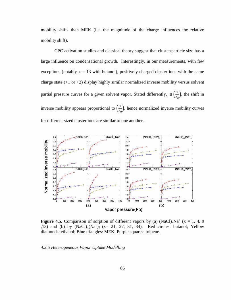
86
mobility shifts than MEK (i.e. the magnitude of the charge influences the relative
mobility shift).
CPC activation studies and classical theory suggest that cluster/particle size has a
large influence on condensational growth. Interestingly, in our measurements, with few
exceptions (notably x = 13 with butanol), positively charged cluster ions with the same
charge state (+1 or +2) display highly similar normalized inverse mobility versus solvent
partial pressure curves for a given solvent vapor. Stated differently, ∆ (1
𝑍𝑥), the shift in
inverse mobility appears proportional to (1
𝑍0), hence normalized inverse mobility curves
for different sized cluster ions are similar to one another.
Figure 4.5. Comparison of sorption of different vapors by (a) (NaCl)xNa+ (x = 1, 4, 9
,13) and (b) by (NaCl)x(Na+)2 (x= 21, 27, 31, 34). Red circles: butanol; Yellow
diamonds: ethanol; Blue triangles: MEK; Purple squares: toluene.
4.3.5 Heterogeneous Vapor Uptake Modelling

87
Observations of inverse mobility versus solvent partial pressure suggest that (1)
sorption is highly vapor molecule structure dependent, (2) sorption is charge state
dependent, and (3) relative mobility shifts brought about by sorption are only weakly
dependent on cluster size. The concavity of the relative mobility versus solvent partial
pressure curves also suggest that results can be fit and parameterized by a vapor molecule
site-specific binding model. This model, (a Langmuir-adsorption based model) is
described by Oberreit et al (D. R. Oberreit et al., 2015), and in it a cluster ion is assumed
to have a maximum number (휁𝑥 ) of sites to which a specific kind of solvent vapor
molecules could bind. The activity coefficient 𝑎𝑥 , defined as the ratio solvent vapor
pressure at the surface of the cluster ion to the solvent saturation vapor pressure at a given
temperature, is adjusted along with 휁𝑥 to fit the data to the model. To perform the
calculation, a unimolecular equilibrium sorption coefficient is defined as:
𝐾𝑒𝑞,𝑔′ =
𝑛𝑔
𝑛𝑔−1 (4.1)
where 𝑛𝑔 and 𝑛𝑔−1 are the number of cluster ions with 𝑔 and 𝑔 − 1 vapor molecules
bound. If cluster ions quickly equilibrate with their surroundings once they enter the
DMA, 𝐾𝑒𝑞,𝑔′ can be treated as a constant at a given saturation ratio 𝑆 and can be
calculated as:
𝐾𝑒𝑞,𝑔′ =
𝑆
𝑎𝑥(𝜁𝑥+1
𝑔− 1) (
𝜇𝑣,𝑔
𝜇𝑣,𝑔−1)1/2
(PA𝑔−1
PA𝑔) 휂[𝜓𝐷,𝑔−1] (4.2)
where PA𝑔 is the projected area of the cluster ion with 𝑔 vapor molecules bound to it,
𝜇𝑣,𝑔 is the reduced mass of the sorbing vapor-cluster ion pair, 휂[𝜓𝐷,𝑔] is an enhancement
factor in vapor-cluster ion collision rate considering the interaction between the charge on

88
the cluster ion and the dipole moments of the sorbing vapor molecule (defined in (D. R.
Oberreit et al., 2015)). For simplicity, here, PA𝑔 is estimated with the bulk material
properties assuming the clusters are spherical. The probability that a cluster ion has g
molecules attached to it is then calculated as:
𝑃𝑔 =𝑛𝑔
𝑛0+∑ 𝑛𝑖𝑖=∞𝑖=1
(4.3)
With the equilibrium coefficients, 𝑃𝑔 can be alternatively expressed as,
𝑃𝑔 =∏ 𝐾𝑒𝑞,𝑗
′𝑔𝑗=1
1+∑ ∏ 𝐾𝑒𝑞,𝑗′𝑗=𝑖
𝑗=1𝑖=∞𝑖=1
(𝑔 ≥ 1) (4.4a)
𝑃𝑔 =1
1+∑ ∏ 𝐾𝑒𝑞,𝑗′𝑗=𝑖
𝑗=1𝑖=∞𝑖=1
(𝑔 = 0) (4.4b)
the average mobility of the cluster ion at a specific saturation ratio of the solvent vapor
can then be determined:
𝑍𝑆,𝑐𝑎𝑙 = ∑ 𝑃𝑔𝑍𝑔𝑔=𝜁𝑥𝑔=0 (4.5)
Given a combination of 휁𝑥 and 𝑎𝑥, the calculated cluster ion mobilities 𝑍𝑆,𝑐𝑎𝑙 are
compared with the mobilities at different saturations ratios for selected ions. A weighted
least square method with weights proportional to the partial pressure range that each data
point represents is used to determine the most appropriate 휁𝑥 and 𝑎𝑥 values. Resultant
fitting parameters for the sorption of butanol, ethanol, MEK and toluene molecules by
both positively and negatively charged cluster ions (NaCl)xNa+ /(NaCl)xCl- (x = 1, 4, 9
,13) are listed in Table 4.1. Selected results of x =4 and x = 9 clusters are shown in Figure
4.6, with other fit results displayed in Figure C1 in Appendix C. For butanol, ethanol and
MEK, the number of available sites on positively charged cluster ions increases with
cluster size, as do the activity coefficients, with the exception of (NaCl)4Na+. For toluene,

89
which shows little uptake by positively charged cluster ions, the activity coefficient is
greater than 1, similar to Kelvin effect included in classical nucleation theory. For
negatively charged cluster ions, the fit parameters do not scale with size, likely because
of structural differences in different sized cluster ions, as evidenced in the results plotted
in Figure 4.2 and Figure 4.4.
Table 4.1. The fitting parameters, determined for (NaCl)xNa+ (positive) and (NaCl)xCl-
(negative) clusters by comparing experiments to Equation (4.1-4.5) predictions.
Solvent
Vapor
Positive Negative
x 𝒂𝒙 x x 𝒂𝒙 x
butanol
1 0.0358 8 1 0.476 9
4 0.0392 12 4 2.50 42
9 0.0606 18 9 1.67 48
13 0.0794 20 13 0.0526 22
ethanol
1 8.03×10⁻³ 7 1 0.0478 6
4 7.24×10⁻³ 9 4 0.200 20
9 9.97×10⁻³ 13 9 0.714 49
13 0.0163 17 13 0.036 10
MEK
1 1.02×10⁻⁴ 4 1 3.33 15
4 1.77×10⁻³ 5 4 0.345 1
9 2.45×10⁻³ 7 9 0.233 3
13 2.92×10⁻³ 9 13 1.67 11
Toluene
1 5.00 24 1 0.286 1
4 5.00 15 4 0.0787 1
9 1.25 12 9 0.120 1
13 3.33 24 13 0.0971 1
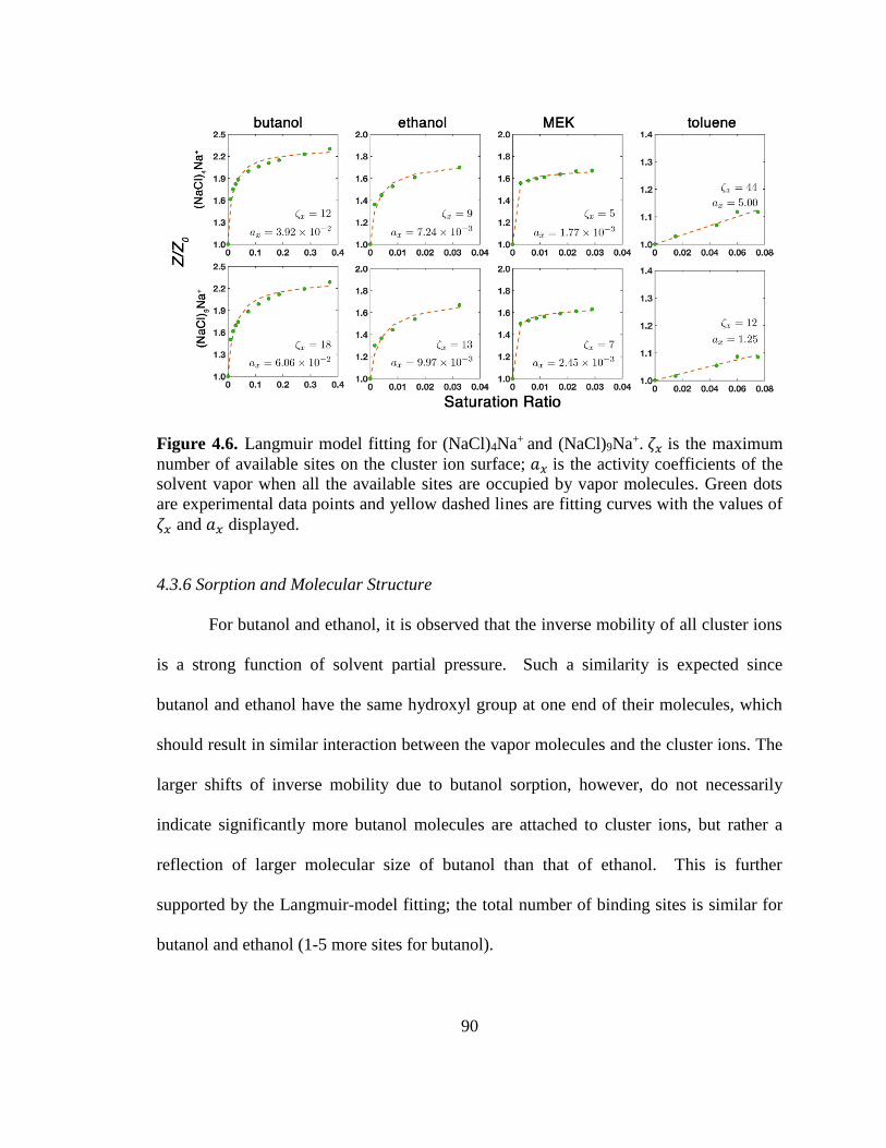
90
Figure 4.6. Langmuir model fitting for (NaCl)4Na+ and (NaCl)9Na+. 휁𝑥 is the maximum
number of available sites on the cluster ion surface; 𝑎𝑥 is the activity coefficients of the
solvent vapor when all the available sites are occupied by vapor molecules. Green dots
are experimental data points and yellow dashed lines are fitting curves with the values of
휁𝑥 and 𝑎𝑥 displayed.
4.3.6 Sorption and Molecular Structure
For butanol and ethanol, it is observed that the inverse mobility of all cluster ions
is a strong function of solvent partial pressure. Such a similarity is expected since
butanol and ethanol have the same hydroxyl group at one end of their molecules, which
should result in similar interaction between the vapor molecules and the cluster ions. The
larger shifts of inverse mobility due to butanol sorption, however, do not necessarily
indicate significantly more butanol molecules are attached to cluster ions, but rather a
reflection of larger molecular size of butanol than that of ethanol. This is further
supported by the Langmuir-model fitting; the total number of binding sites is similar for
butanol and ethanol (1-5 more sites for butanol).
91
Meanwhile, MEK sorbs much more prevalently to positively charged cluster ions
than to their negative counterparts in the pressure range considered. We speculate that
such charge polarity discrimination could arise from electrostatic interactions between the
cluster ions and MEK molecules. The carbonyl group in MEK molecules has a negative
partial charge on the oxygen atom, which could facilitate adsorption by positively
charged cluster ions. However, the positive partial charge on the carbon atom (in C=O) is
less pronounced, as this net charge is distributed to neighboring carbon ions.
Unlike the other three solvents that contain strongly polar functional groups,
toluene has less pronounced effect on cluster ion mobilities for all charge states. We
speculate this is due to the lack of polar functional groups in toluene. It is also possible
that the smaller dipole moment of toluene (0.36 D) compared to the other solvent vapor
(butanol~1.66 D, ethanol ~1.69 D, MEK~2.76 D) could cause such differences in
sorption. To ascertain if this is the case, we conducted experiments with chlorobutane as
solvent vapor. Chlorobutane has a larger dipole moment (1.90 D) than both butanol and
ethanol and should therefore be readily adsorbed by cluster ions if the dipole moment
plays a central role. However, chlorobutane vapor induces inverse mobility shift less than
10% for all the cluster ions within the pressure range 0-300 Pa (as shown in Figure C2 in
Appendix C), suggesting that it is not simply dipole moment that governs sorption.
4.4 Conclusions
We used a differential mobility analyzer-mass spectrometry to investigate organic
vapor uptake by nanometer scale particles, i.e. sodium chloride cluster ions. Results for
92
four solvent vapors (butanol, ethanol, MEK and toluene) are displayed and were
compared. Based on this study, we make the following concluding remarks:
1. Overwhelmingly, cluster ion charge polarity and the molecular structures of the
vapor molecules are found to control the extent of vapor uptake, in qualitative
agreement with previous CPC activation efficiency studies which strong chemical
composition and charge polarity influences. All tested vapors appear to sorb to
ions when present at partial pressure of 102 Pa, irrespective of their saturation
vapor pressure. Cluster size is found to have a much smaller influence on uptake
facilitated inverse mobility shift (when normalized by the dry inverse mobility)
than vapor molecular structure and ion polarity.
2. While cluster “size” does not appear to strongly influence vapor sorption, cluster
structure appears to have a pronounced influence. In particular, for (NaCl)xCl- x
=7, 8, 9 group (among others), under dry conditions the measured inverse
mobility does not scale with cluster mass, suggesting that clusters differing by one
cation-anion pair have disparate structures from one another. For these clusters
we also find unique extents of uptake.
3. Taking (1) and (2) into account, our measurement suggest that the earliest of
uptake are not dependent purely on cluster “size”, rather electrostatic interactions
and molecular/cluster structure govern vapor sorption. We suggest that in the
future design of condensers and condensation particle counters for the 1 nm size
range, that activation efficiencies (which hinge upon particles/clusters first
sorbing vapor) the activation efficiency not be reported solely as a function of
mobility equivalent size, but should be examined for a variety of clusters with
93
variable structures. It is unlikely that any single cluster type can serve as
surrogate for all clusters/particles of interest in different environments.
4. The vapor-scavenging behavior observed in this work by cluster ions, even at the
~100 parts per million vapor concentration level implies that the presence of
solvent vapor will influence ion properties in most environments, which has
implications not only growth on ions but also in the application of ions in
charging pre-existing particles. Specifically, trace amounts of vapors might have
an impact on the stationary charge distribution attained of aerosol neutralizers, as
has been observed experimentally (Steiner & Reischl, 2012). This may be
particularly problematic in studies where particles are aerosolized via organic
solvent sprays and residue solvent in the vapor phase is likely.
94
Chapter 5: Mass, Momentum, and Energy Transfer in Supersonic
Aerosol Deposition Processes
Abstract: Aerosol deposition (AD) has emerged as a novel additive manufacturing
(AM) method for surface coating and thin film production. In contrast to cold
spray, AD does not require pressurized gas, works at room temperature and is
frequently used to deposit sub-micron particles. It is generally acknowledged that
the instantaneous particle speed upon impaction is critical to controlling
coating/film properties such as porosity, and mitigating particle bounce during
deposition. Therefore, converging-diverging nozzles are often employed in AD to
accelerate particles to the desirable impaction speed. In this work, we simulated
flow field profiles as well as particle trajectories for typical AD working conditions
for a slit type converging-diverging nozzle. In examining the flow filed profile, we
show that the velocity, pressure profile as well as shock structure are sensitive to the
upstream and downstream operating pressures of the nozzle, which in turn affects
particle impaction speed. To aid particle trajectory simulations, we trained a neural
network to predict drag force on the particles based on existing experimental data,
theoretical limits and simulation results obtained by direct simulation of Monte
Carlos (DSMC). The neural network based drag law shows better agreement with
the DSMC simulation data. Particle trajectory simulation results reveal that for a
given particle density, there exists an optimal particle diameter to maximize particle
impaction speed, as well as a diameter to maximize particle initial focusing, though
these two diameters are typically not equal. We developed a framework that can be

95
used to evaluate the position-dependent mass, momentum and kinetic energy flux to
the deposition substrate for any aerosol size distribution upstream the nozzle. It is
shown for typical aerosol concentrations achievable in laboratory, the kinetic energy
flux can approach a magnitude normally observed in convective heat transfer with
phase change due to particle inertial focusing.
5.1 Introduction
Aerosol deposition (AD) has emerged as an additive manufacturing method for
coating and thin film production (Akedo, 2006, 2008; Hanft et al., 2015; C. Huang et al.,
2007; M. W. Lee et al., 2011; Park et al., 2014; Park et al., 2017). Distinct from other
particle deposition methods, such as thermal and cold spray (Stoltenhoff, Kreye, &
Richter, 2002; Yin, Meyer, Li, Liao, & Lupoi, 2016), AD can function at room
temperature and does not require highly pressurized gas (Adachi, Okuyama, Kousaka, &
Tanaka, 1988; Hanft et al., 2015); this facilitates deposition onto low-melting point
materials with simpler manufacturing devices. The AD process involves accelerating
particles with a compressible, high-speed carrier gas, leading to particle impaction at
supersonic speeds and reduced pressure, with the potential for both particle heating as
well as plastic deformation upon collision with the substrate (while the substrate itself is
relatively undisturbed). It is generally acknowledged that high particle speed during
impaction is critical to control coating/film properties such as porosity, and to mitigate
particle bounce upon deposition (Hamid Assadi, Gärtner, Stoltenhoff, & Kreye, 2003;
Yin et al., 2016). To this end, converging-diverging nozzles (i.e. de Laval nozzles) are

96
frequently used, as such nozzles enable the acceleration of flow and of particles to
supersonic speeds within the nozzles themselves.
Though considerable effort has been devoted to simulation of particle trajectories
within converging-diverging nozzles and to estimate impaction speeds in particle
deposition systems (Abouali & Ahmadi, 2005; C. Huang et al., 2007; Katanoda,
Fukuhara, & Iino, 2007; M.-W. Lee et al., 2011), many critical aspects the AD process
remain uninvestigated. First, the drag force of the carrier gas on particles needs to be
carefully considered in designing AD systems. As particles traverse through the nozzle,
rapid gas rarefication and densification (due to shock formation) can lead to particle
Knudsen number (Kn) variations by as much as ~102, hence the drag regime rapidly
varies between the ballistic/free molecular and continuum limits. In addition, due to gas
stagnation close to the substrate or insufficient particle acceleration, particle Mach
numbers (Ma, based on relative speed of gas and particles) can exceed unity, with
potential shock formation close to the particle surface (Fernández de la Mora, Rao, &
McMurry, 1990). Modeling of particle trajectories, therefore, requires a drag law that is
valid for a wide range of Kn and Ma. To date, many models of the AD process do not
appropriately consider the Knudsen and Mach number evolution for particles (C. Huang
et al., 2007; G. Huang, Gu, Li, Xing, & Wang, 2014; Johnson, Schwer, Park, Park, &
Gorzkowski, 2017), and for those where this is considered (Ning, Wang, Ma, & Kim,
2010), the most widely used particle drag correlation is that proposed by Henderson
(Henderson, 1976). The basis dataset for Henderson’s correlation is unfortunately
incomplete; in particular, it does not span the Kn and Ma number ranges critical to AD
systems operating at reduced pressure. For example, submicrometer particles typically lie
97
within the transition regime (0.1<Kn<10), and can have Mach numbers between 0 and 3
during deposition; however, a large fraction of the data utilized in Henderson’s
correlation in this Kn range were collected at extremely low Mach number, i.e. Ma ∈
(5 × 10⁻⁷, 6 × 10⁻⁶), and there are few data points with Kn of order 10-1 and Ma > 1
(Bailey & Hiatt, 1971) .
Another aspect to be explored in AD relates to how operating conditions of the
nozzle influences particle impaction speed. Relevant factors, such as gas temperature and
composition, substrate position and particle size, have been examined closely for cold
spray process (Champagne, Helfritch, Dinavahi, & Leyman, 2011; Katanoda et al., 2007;
M.-W. Lee et al., 2011; Yin et al., 2016), wherein the upstream pressures are typically on
the order of 106 Pa, the downstream pressure is atmospheric pressure, and the particles
are tens of micrometers in diameter. The AD process, conversely, is characterized by
atmospheric upstream pressure and reduced downstream pressure, and has significantly
larger gas rarefaction effects. Because of low downstream pressures AD has the potential
for application with submicrometer and nano-sized (<100nm) particles (Adachi et al.,
1988; Fernández de la Mora et al., 1990; Rao et al., 1998), though this is not commonly
considered in AD design.
A final concern regarding the AD process is the influence of the input particle size
distribution function on linewidth/mass deposition profile, as well as momentum and
energy fluxes to the substrate. Ultimately, aerosol deposition is an inertial process.
Inertial motion of particles is not only known to be highly particle size dependent, but
also leads to lateral focusing of particles (de Juan & Fernandez de la Mora, 1998; X. L.
Wang, Kruis, & McMurry, 2005), i.e. the depositing particle linewidths will be highly

98
particle size specific, and there will be an optimally focused particle size which has the
minimal deposition linewidth. Such focusing effects, coupled with polydisperse size
distributions, dramatically impact the mass, momentum, and energy flux distributions
over the substrate area, though this has not been described previously.
Here, we apply a combined computational fluid dynamics-particle trajectory
model to better examine particle mass, momentum, and energy transfer to substrates in
aerosol deposition. Specifically, in our modeling we examine a slit shaped converging-
diverging nozzle under conditions applicable to AD. Particle trajectories are simulated
using drag coefficients derived from a neural network (to correct the drag coefficient
relationship) incorporating new direct simulation Monte Carlo data to compute particle
drag coefficients for Ma ∈ (0, 5) over a wide Kn number range. Particle trajectories and
spatial distributions at impaction are examined varying particle size and density. Finally,
mass, momentum, and energy flux distribution equations are developed and applied to
examine how the spatial distribution of depositing particles affects the overall mass
deposition rate, particle momentum flux, and impinging particle kinetic energy flux.
5.2 Computational Methods
5.2.1 Nozzle Geometry and Simulation Domain
The nozzle geometry used in this study is shown in Figure 5.1. The nozzle is a
slit-shaped, converging-diverging de Laval nozzle, which would be suitable for
deposition of coatings via rastering of the substrate.(Hanft et al., 2015) It has an inlet
width of 4.4 mm and an outlet width of 2 mm, as well as a throat width of 0.2 mm. The
converging section of the nozzle has a length of 2.5 cm, while the diverging section is 3.5

99
cm. A 20 mm width, flat substrate is placed 6 mm below the nozzle outlet; the chamber
housing the substrate is 44 mm in width.
Figure 5.1. Nozzle geometry and simulation domain.
5.2.2 Computational Fluid Dynamics Simulation
We employed finite volume simulations using ANSYS Fluent 18, solving the two
dimensional compressible Navier-Stokes equations to obtain the fluid flow profile under
steady conditions coupled with solution to the energy equation. We elected to use two-
dimensional simulations in consideration of the high nozzle cross section aspect ratio
(near 102) commonly utilized in AD with slit-type nozzles; in this instance two-
dimensional simulation should provide reasonable accuracy in a more computationally
efficient manner than a fully three-dimensional model. A turbulence model was
employed because at the nozzle throat, the hydraulic diameter based Reynolds number is
~5×10³ with atmospheric pressure upstream, hence a modest degree of turbulence may
arise in the flow. Prior work has shown that the SST 𝑘 − 𝜔 turbulence model (Menter,
1994) is accurate in simulating compressible flows in converging-diverging nozzles

100
(Balabel, Hegab, Nasr, & El-Behery, 2011); thus, we chose this model to account for
turbulent dissipation in flow-profile simulations. The governing equations for continuity,
momentum transfer, and energy using this model are provided in (Ding, Wang, & Wang,
2017; Fluent, 2009) and noted in the Appendix E.
It is important in AD fluid flow simulations to have a sufficiently high node
density near the substrate to resolve the shock structure at the substrate surface. A grid
independence study was carried out to determine the number of grid points required to
fully resolve the flow profile. In this study, we simulated half of the nozzle geometry
(because of symmetry conditions) with 1.0×10⁶, 1.6×10⁶, and 3.0×10⁶ nodes. We
observed negligible difference in simulation velocity and pressure fields between these
three simulations, indicating all were appropriate in modeling the flow and pressure
fields. In all simulations the gas modeled was nitrogen (N2); its viscosity varied with
temperature in accordance with the Sutherland equation, as noted in Appendix G. The
boundary conditions were set as follows: (1) the no-slip condition was invoked at all solid
walls and the substrate, and all solid boundaries were treated as adiabatic; (2) the inlet
temperature was set to 300K, at a stagnation pressure of either 190 or 760 Torr; and (3)
the outlet static pressure (at the boundaries, Figure 5.1) was set to either 1 Torr or 10
Torr. At the inlet the flow direction was set to be normal to the boundary and the
turbulence intensity was set to be 1% (low turbulence). Simulations were run until the
scaled residual reached the following criteria, which are commonplace in ANSYS Fluent
simulations (Fluent, 2009): continuity< 1 × 10⁻⁵ , x-velocity< 1 × 10⁻⁵, y-velocity<
1 × 10⁻⁵ , energy ≤ 1 × 10⁻⁵ , 𝑘 < 5 × 10⁻⁵ , and 𝜔 < 1 × 10⁻⁶ . The difference

101
between inlet and outlet mass flow rates were checked as another criterion for
convergence: for all cases examined, the flowrate differences were less 0.1%.
5.2.3 Particle Trajectory Simulations
We assumed one way coupling between the fluid and the particles, i.e. the
presence of particles was assumed to have negligible effect on the flow profile. To
estimate particle impaction velocity and flux distribution to the substrate, particles of
prescribed diameter and density were released uniformly along the inlet boundary of the
nozzle. The examined particle diameters range from 3 nm to 10 𝜇m, and two densities
were selected: 2650 kg m-3 and 8960 kg m-3, which correspond to silica and copper,
respectively. Particle Brownian (thermal) motion was not considered as this effect is
expected to be small relative to the influences of flow and inertia. (Lindquist, Pui, &
Hogan Jr, 2014) Additionally, as shown in the Results & Discussion section, for the
simulated flow conditions, only particles > 15 nm impact upon the substrate (for copper),
for which Brownian motion would certainly minimally impact trajectories.
For trajectory calculations, user-defined functions were incorporated in Fluent’s
discrete phase model (DPM). At each time step, the gas properties (specifically the
velocity vector, the temperature, and the pressure) were sampled from the cell in which a
particle was located. These properties were then used to compute the drag force on the
particles using user defined drag laws. The equation of motion for a particle is expressed
as:
𝜌𝑝𝜋
6𝑑𝑝
3 𝑑𝑣𝑟
𝑑𝑡= −
1
2𝜌𝑔‖𝑣𝑟 ‖2𝐴𝑝𝐶𝑑
𝑣𝑟
‖𝑣𝑟 ‖ (5.1)

102
where 𝑣𝑟 is the relative velocity vector between the particle and fluid, 𝜌𝑝 is the
particle density, 𝑑𝑝 is the particle diameter, 𝜌𝑔 is the gas density, 𝐴𝑝 is the particle cross
sectional area, and 𝐶𝑑 is the drag coefficient. Correlations have been developed for 𝐶𝑑 in
different Mach number and Knudsen number regimes. We review selected regimes here,
showing that until recently, there were limited results in the Ma and Kn ranges of interest
for AD. In the limit of particle Mach number 𝑀𝑎 → 0, the Cunningham correction factor
is used to modify Stokes’s law to account for the rarefaction effect. 𝐶𝑑,𝐶 , is given by
(Davies, 1945):
𝐶𝑑,𝐶 =24
𝑅𝑒(1 + 2𝐾𝑛 [1.257 + 0.4exp (−
0.55
𝐾𝑛)])
−1
(5.2)
where the subscript “C” denotes it is Cunningham’s correlation, and 𝑅𝑒 =𝜌𝑔‖𝑣𝑟 ‖𝑑𝑝
𝜇 and
𝐾𝑛 =𝜆
𝑑𝑝 are particle Reynolds and Knudsen number, respectively (𝜇 is the gas dynamic
viscosity and 𝜆 is the gas hard sphere mean free path, calculated as noted in Appendix G).
We note that this definition of Kn, used throughout this manuscript, is is in agreement
with some of the previous work on particle drag with direct simulation Monte
Carlo(Singh & Schwartzentruber, 2017) (Macrossan, 2006), but is distinct from the
commonly used definition normalizing by particle radius (C. L. Zhang, Thajudeen,
Larriba, Schwartzentruber, & Hogan, 2012) and common equations have been adjusted
accordingly. For particles in the free molecular regime (𝐾𝑛 → ∞) , assuming all gas
molecules are reflected diffusely after colliding with the particle surface, an analytical
expression for 𝐶𝑑 was derived by Patterson (Patterson, 1971):
𝐶𝑑,𝑃 =2
𝑆3[2𝑆2+1
2√𝜋exp(−𝑆2) + (
4𝑆4+4𝑆2−1
4𝑆) erf(𝑆)] +
2√𝜋
3𝑆(
𝑇𝑝
𝑇∞)
1
2 (5.3)
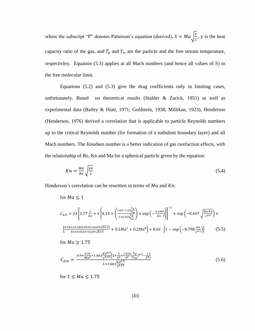
103
where the subscript “P” denotes Patterson’s equation (derived), 𝑆 = 𝑀𝑎√𝛾
2 , 𝛾 is the heat
capacity ratio of the gas, and 𝑇𝑝 and 𝑇∞ are the particle and the free stream temperature,
respectivley. Equation (5.3) applies at all Mach numbers (and hence all values of S) in
the free molecular limit.
Equations (5.2) and (5.3) give the drag coefficients only in limiting cases,
unfortunately. Based on theoretical results (Stalder & Zurick, 1951) as well as
experimental data (Bailey & Hiatt, 1971; Goldstein, 1938; Millikan, 1923), Henderson
(Henderson, 1976) derived a correlation that is applicable to particle Reynolds numbers
up to the critical Reynolds number (for formation of a turbulent boundary layer) and all
Mach numbers. The Knudsen number is a better indication of gas rarefaction effects, with
the relationship of Re, Kn and Ma for a spherical particle given by the equation:
𝐾𝑛 =𝑀𝑎
𝑅𝑒√
𝛾𝜋
2 (5.4)
Henderson’s correlation can be rewritten in terms of 𝑀𝑎 and 𝐾𝑛:
for 𝑀𝑎 ≤ 1
𝐶𝑑,𝐻 = 24 [1.77𝑆
𝐾𝑛+ 𝑆 {4.33 + (
3.65−1.53𝑇𝑝
𝑇∞
1+0.353𝑇𝑝
𝑇∞
) × exp (−0.438
𝐾𝑛)}]
−1
+ exp (−0.447 √𝑀𝑎∙𝐾𝑛
𝛾0.5 ) ×
[4.5𝐾𝑛+0.38(0.053𝑆+0.639√𝐾𝑛∙𝑆)
𝐾𝑛+0.053𝑆+0.639√𝐾𝑛∙𝑆+ 0.1𝑀𝑎2 + 0.2𝑀𝑎8] + 0.6𝑆 ∙ [1 − exp (−0.798
𝐾𝑛
𝛾0.5)] (5.5)
for 𝑀𝑎 ≥ 1.75
𝐶𝑑,𝐻 = 0.9+
0.34
𝑀𝑎2+1.661𝐾𝑛0.5
𝛾0.25 [2+2
𝑆2+1.058
𝑆2 (𝑇𝑝
𝑇∞)0.5−
1
𝑆4]
1+1.661𝐾𝑛0.5
𝛾0.25
(5.6)
for 1 ≤ 𝑀𝑎 ≤ 1.75
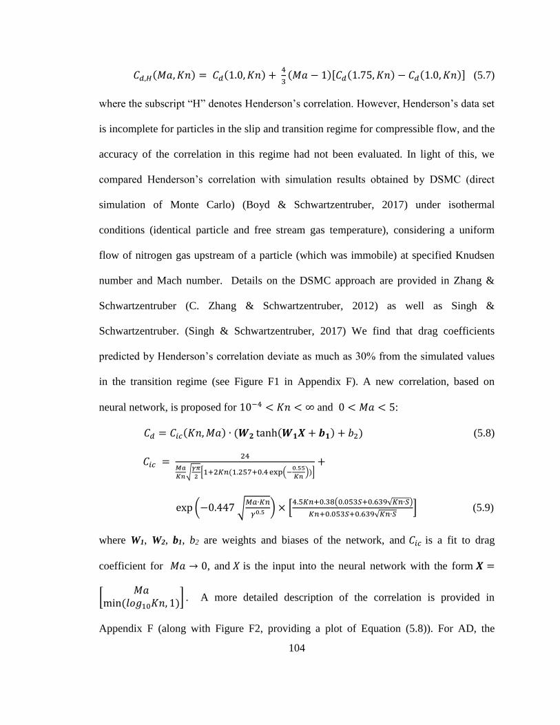
104
𝐶𝑑,𝐻(𝑀𝑎, 𝐾𝑛) = 𝐶𝑑(1.0, 𝐾𝑛) + 4
3(𝑀𝑎 − 1)[𝐶𝑑(1.75, 𝐾𝑛) − 𝐶𝑑(1.0, 𝐾𝑛)] (5.7)
where the subscript “H” denotes Henderson’s correlation. However, Henderson’s data set
is incomplete for particles in the slip and transition regime for compressible flow, and the
accuracy of the correlation in this regime had not been evaluated. In light of this, we
compared Henderson’s correlation with simulation results obtained by DSMC (direct
simulation of Monte Carlo) (Boyd & Schwartzentruber, 2017) under isothermal
conditions (identical particle and free stream gas temperature), considering a uniform
flow of nitrogen gas upstream of a particle (which was immobile) at specified Knudsen
number and Mach number. Details on the DSMC approach are provided in Zhang &
Schwartzentruber (C. Zhang & Schwartzentruber, 2012) as well as Singh &
Schwartzentruber. (Singh & Schwartzentruber, 2017) We find that drag coefficients
predicted by Henderson’s correlation deviate as much as 30% from the simulated values
in the transition regime (see Figure F1 in Appendix F). A new correlation, based on
neural network, is proposed for 10−4 < 𝐾𝑛 < ∞ and 0 < 𝑀𝑎 < 5:
𝐶𝑑 = 𝐶𝑖𝑐(𝐾𝑛,𝑀𝑎) ∙ (𝑾𝟐 tanh(𝑾𝟏𝑿 + 𝒃𝟏) + 𝑏2) (5.8)
𝐶𝑖𝑐 = 24
𝑀𝑎
𝐾𝑛√
𝛾𝜋
2[1+2𝐾𝑛(1.257+0.4exp(−
0.55
𝐾𝑛))]
+
exp (−0.447 √𝑀𝑎∙𝐾𝑛
𝛾0.5 ) × [4.5𝐾𝑛+0.38(0.053𝑆+0.639√𝐾𝑛∙𝑆)
𝐾𝑛+0.053𝑆+0.639√𝐾𝑛∙𝑆] (5.9)
where W1, W2, b1, b2 are weights and biases of the network, and 𝐶𝑖𝑐 is a fit to drag
coefficient for 𝑀𝑎 → 0, and 𝑋 is the input into the neural network with the form 𝑿 =
[𝑀𝑎
min (𝑙𝑜𝑔10𝐾𝑛, 1)] . A more detailed description of the correlation is provided in
Appendix F (along with Figure F2, providing a plot of Equation (5.8)). For AD, the

105
particles of interest lie in the regime of 10−4 < 𝐾𝑛 < ∞ and 0 < 𝑀𝑎 < 5. In light of
this, the particle drag coefficients are calculated with Equation (5.8) and (5.9) throughout
this work.
5.3 Results & Discussion
In total, we simulate the velocity and pressure fields for a de Laval-type AD
system and examine particle trajectories in the 3 nm – 10 𝜇𝑚 range using drag
coefficients determined for conditions relevant to AD. We first present results of flow
field simulations, following by evaluation of the impaction velocities for particles of two
different densities (under all three flow conditions). Finally, using copper particles as a
model we examine the deposition distribution functions (over the substrate area) and
calculate location dependent mass fluxes, momentum fluxes and energy fluxes for model
particle size distribution functions.
5.3.1 Simulation results of flow properties
Though most AD systems function with atmospheric pressure upstream (Akedo,
2006; Akedo & Lebedev, 1999; Muneyasu, Tetsuo, & Jun, 2017), variable pressure is
worthy of examination as it is possible to optimize the particle deposition process by
varying upstream and downstream pressures (Holman & Kortshagen, 2010; Thimsen et
al., 2014). In addition, the variability of flow properties brought about by operating
conditions provides useful information in the optimization of nozzle design. The
simulated operating conditions are summarized in Table 5.1, along with flow properties
calculated by the isentropic, one-dimensional nozzle theory (Saad, 1985) for comparison.
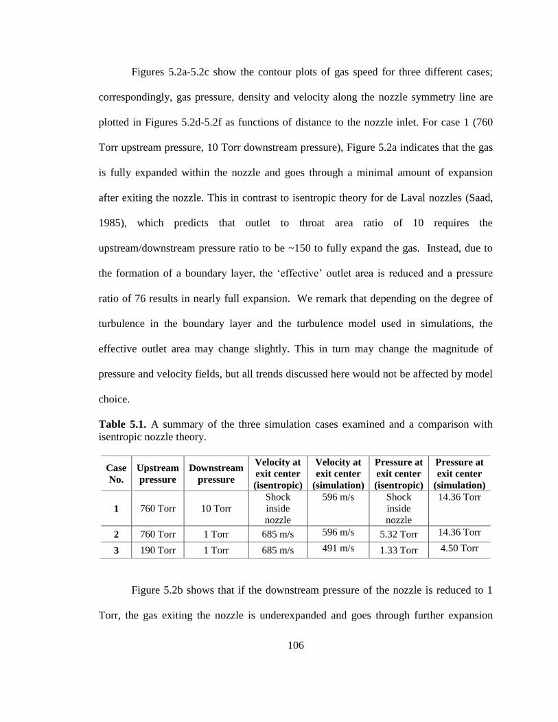
106
Figures 5.2a-5.2c show the contour plots of gas speed for three different cases;
correspondingly, gas pressure, density and velocity along the nozzle symmetry line are
plotted in Figures 5.2d-5.2f as functions of distance to the nozzle inlet. For case 1 (760
Torr upstream pressure, 10 Torr downstream pressure), Figure 5.2a indicates that the gas
is fully expanded within the nozzle and goes through a minimal amount of expansion
after exiting the nozzle. This in contrast to isentropic theory for de Laval nozzles (Saad,
1985), which predicts that outlet to throat area ratio of 10 requires the
upstream/downstream pressure ratio to be ~150 to fully expand the gas. Instead, due to
the formation of a boundary layer, the ‘effective’ outlet area is reduced and a pressure
ratio of 76 results in nearly full expansion. We remark that depending on the degree of
turbulence in the boundary layer and the turbulence model used in simulations, the
effective outlet area may change slightly. This in turn may change the magnitude of
pressure and velocity fields, but all trends discussed here would not be affected by model
choice.
Table 5.1. A summary of the three simulation cases examined and a comparison with
isentropic nozzle theory.
Case
No.
Upstream
pressure
Downstream
pressure
Velocity at
exit center
(isentropic)
Velocity at
exit center
(simulation)
Pressure at
exit center
(isentropic)
Pressure at
exit center
(simulation)
1 760 Torr 10 Torr
Shock
inside
nozzle
596 m/s Shock
inside
nozzle
14.36 Torr
2 760 Torr 1 Torr 685 m/s 596 m/s 5.32 Torr 14.36 Torr
3 190 Torr 1 Torr 685 m/s 491 m/s 1.33 Torr 4.50 Torr
Figure 5.2b shows that if the downstream pressure of the nozzle is reduced to 1
Torr, the gas exiting the nozzle is underexpanded and goes through further expansion
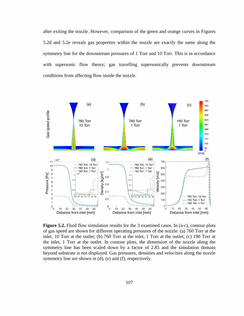
107
after exiting the nozzle. However, comparison of the green and orange curves in Figures
5.2d and 5.2e reveals gas properties within the nozzle are exactly the same along the
symmetry line for the downstream pressures of 1 Torr and 10 Torr. This is in accordance
with supersonic flow theory; gas travelling supersonically prevents downstream
conditions from affecting flow inside the nozzle.
Figure 5.2. Fluid flow simulation results for the 3 examined cases. In (a-c), contour plots
of gas speed are shown for different operating pressures of the nozzle: (a) 760 Torr at the
inlet, 10 Torr at the outlet; (b) 760 Torr at the inlet, 1 Torr at the outlet; (c) 190 Torr at
the inlet, 1 Torr at the outlet. In contour plots, the dimension of the nozzle along the
symmetry line has been scaled down by a factor of 2.85 and the simulation domain
beyond substrate is not displayed. Gas pressures, densities and velocities along the nozzle
symmetry line are shown in (d), (e) and (f), respectively.
108
For case 3, Figure 5.2c reveals that as the upstream pressure is reduced, the flow
speed within the nozzle is also reduced. This is in contradiction to the isentropic theory
(c.f. Table 5.1), but is again attributable to viscous effects in the flow. The gas viscosity
is independent of pressure, hence reducing the upstream pressure from 760 Torr to 190
Torr does not result in a decrease of viscous effects given the same velocity gradient.
Therefore, a higher fraction of the pressure head must act to compensate for viscous
effects in case 3 than in the higher upstream pressure cases; this results in a less
accelerated gas. Additional pressure and temperature contour plots are shown for case 1
in Figure H1in Appendix H; qualitatively similar plots are obtained for other cases.
Figure 5.2 also provides useful information regarding the post-shock region, i.e.
the region close to the substrate, as well as how operating pressures affect gas properties
within this region. As the gas traverses through the shock, its properties change
drastically, which is clearly evident in Figures 5.2d-5.2f. With static pressure as an
example, changing the downstream pressure from 10 Torr to 1 Torr decreases the
pressure in post-shock region from ~113 Torr to ~37 Torr. Simultaneously, the thickness
of the post shock region (distance between the shock and the substrate) changes from
~0.68 mm to ~1.65 mm. Reducing the upstream operation pressure from 760 Torr to 190
Torr has a similar effect. The pressure in the post-shock region changes from ~37 Torr to
~6.75 Torr, and the thickness of the post-shock region increases form ~1.65mm to 2.25
mm. These results highlight the need for a drag coefficient correlation that is accurate
over the wide range of particle Knudsen numbers and relative gas-particle Mach numbers
caused by nozzle expansion and compression near the substrate. Figure H2 shows
selected plots of particle Knudsen and Mach numbers (expressed as the relative particle
109
velocity to speed of sound ratio) along the center line for case 1 (copper particles). With
the exception of the largest particles examined (10 𝜇𝑚 and larger), the Mach number is
smaller than unity for particles until they approach the shock; however, for smaller
particles, as they enter the shock the Mach number exceeds 1.0. Particle Knudsen
numbers span more than one order of magnitude (for a given particle diameter) as they
traverse the nozzle. The smallest particles examined reach Knudsen numbers above 101,
while the Knudsen numbers of the largest particles remain below 10-1. The effects of this
unique Kn, Ma range on particle deposition are discussed in the next section.
5.3.2 Particle Impaction Simulation Results
Particle impaction speed at the substrate surface is of critical importance in the
AD processes; it appears to be directly related to particle adhesion, plastic deformation,
and is likely the key parameter governing the resulting coating/film properties in AD
(Akedo, 2006; Champagne et al., 2011; Hanft et al., 2015). For trajectory calculations,
utilizing the simulated flow fields, 100 particles of prescribed size and density were
released with their initial positions equally spaced along the nozzle inlet. The velocities
and positions of the particles were recorded until they were either trapped by a wall or
they escaped the simulation domain.

110
Figure 5.3. Particle trajectory simulation results for copper particles for case 1. (a) The
particle impaction efficiency as a function of particle diameter. (b) Average particle
impact speed and x-velocity (i.e. perpendicular to the substrate) as a function of particle
diameter. (c) Impact x-velocity and impact position for different particles diameters. (d)
Particle impaction linewidth for different diameter. Particle impaction linewidth is
defined as four times the average distance of particle impaction point from the center of
the substrate.
We first present particle trajectory results in detail for copper particles traversing
the flow field of case 1 (760 Torr upstream pressure, 10 Torr downstream pressure), with
results summarized in Figures 5.3a-5.3d. Specifically, Figure 5.3a shows the deposition
efficiency (defined as the fraction of particles impacting upon the substrate) as a function
of particle diameter. Both small particles (𝑑𝑝 < 16𝑛𝑚) and large particles (𝑑𝑝 > 5𝜇𝑚)
111
have low impaction efficiencies while particles intermediate to these diameters impact
with perfect efficiency. For small particles, the drag force on particles is high compared
to particle inertia, as a result, sufficiently small particles tend to follow gas stream lines in
the post-shock region and escape the simulation domain (this phenomenon is observed in
all particle inertial separation systems (Fernandez de la Mora, Hering, Rao, & McMurry,
1990; Marple & Willeke, 1976)). Conversely, particles larger than 5𝜇𝑚 do not leave the
simulation domain, but as a result of high inertia compared to drag force they cross the
nozzle symmetry line at the throat and collide with the nozzle wall on the side opposite to
their release point. Sample particle trajectories are provided in Figure H3. Figure 5.3b
shows average particle impact velocity along with its x-component for different particle
diameters. The average particle impaction velocity initially increases with particle
diameter and then decreases with it, with a maximum impact speed for ~300 nm diameter
particles. To our knowledge, this is first direct calculation revealing that particles of
highest impaction speed in AD can be in the submicrometer size range, as most work has
focused on supermicrometer particles. As particles traverse through the nozzle, they are
first accelerated by the carrier gas and are then decelerated by stagnated gas in the post-
shock region, just prior to impaction. Though particles of small sizes tend to be fully
accelerated in the nozzle, they are decelerated significantly in the post-shock region,
where the gas has an x-velocity approaching 0 (refer to Figure 5.2f). In contrast,
sufficiently large particles are less affected by the post-shock region, but are not fully
accelerated inside the nozzle. The net result of the acceleration-deceleration process is an
optimal particle size that has the highest impact velocity. This phenomenon has been
reported in simulations of cold spray (H. Assadi et al., 2011), though maximum
112
deposition speed was found for significantly larger particles; this is because in high
pressure cold spray, the effects of the post-shock are most pronounced but larger particles
are better accelerated upstream (i.e. the drag coefficient is larger in cold spray). We can
therefore conclude that the existence of an optimum in particle diameter for the impact
speed is universal in nozzle based deposition systems, though the particle diameter
impacting with highest speed is adjustable by adjusting upstream and downstream
pressures.
Figure 5.3c shows the lateral position r (i.e. distance between the substrate center
and the particle impaction point) and the x-velocity for each deposited particle at selected
particle diameters. For 𝑑𝑝 = 20 𝑛𝑚, the particle impact positions are relatively dispersed
in r. As particle diameter increases, the dispersity of particle impact positions decreases
substantially, reaching a minimum at 𝑑𝑝 = 1 𝜇𝑚. This is attributable to inertial focusing
of particles.(de Juan & Fernandez de la Mora, 1998; X. L. Wang et al., 2005) Inertial
focusing occurs when particles are first directed towards the substrate center in the
converging section the nozzle, but, because of their inertia, they are not sufficiently
accelerated laterally outward in the diverging section. Focused particles hence deposit
close to the substrate center, independent of their initial position. For the examined
nozzle and flow conditions at diameters below 1 𝜇𝑚, the particles are underfocused,
hence the deposition linewidth increases with decreasing particle diameter. Beyond a
diameter of 1 𝜇𝑚 particles are overfocused; overfocusing occurs when particles are
inertially directed across the symmetry axis of the nozzle in the converging section. An
alternative representation of focusing is shown in Figure 5.3d, which is a plot of the
impaction linewidth as a function of particle diameter. Impaction linewidth is defined as
113
4 times the average impact position (accounting for the symmetry condition). Evidenced
in the figure, an optimal diameter (1 𝜇𝑚) for particle focusing exists and the nozzle
functions as an aerodynamic lens (X. L. Wang et al., 2005). We note that for 𝑑𝑝 > 5 𝜇𝑚,
the impaction width is approximately 0.8 mm. For these particle diameters the impaction
efficiencies are less than 100%, and the impaction linewidth only reflects the dispersity of
transmitted particles (i.e. the linewidth is reduced due to particle loss upstream). While
focusing is a known phenomenon, commonly used in concentrating aerosol particles for
chemical analysis (Jayne et al., 2000; Liu, Ziemann, Kittelson, & McMurry, 1995;
Mallina, Wexler, Rhoads, & Johnston, 2000; Middha & Wexler, 2003), it has not been
examined closely in either cold spray or aerosol deposition. However, our results
indicate that the focusing effect is pronounced in AD with converging-diverging nozzles,
and although the optimally focused diameter of 1 𝜇𝑚 is system specific, a maximally
focused diameter will exist in all gas phase particle inertial deposition systems (similarly,
smaller particles will be underfocused and sufficiently large particles will be
overfocused). Through focusing, the input particle size distribution in any deposition
system has a strong influence on the overall linewidth, as well as the momentum and
kinetic energy flux distributions to the substrate. We examine these effects subsequently
using test polydisperse particle size distribution functions. We also remark that focusing
would be adversely affected were the turbulence intensity within the flow to reach
appreciably high levels; this would lead to a distribution of particle trajectories (for a
given diameter and initial position) as opposed to deterministic trajectories.
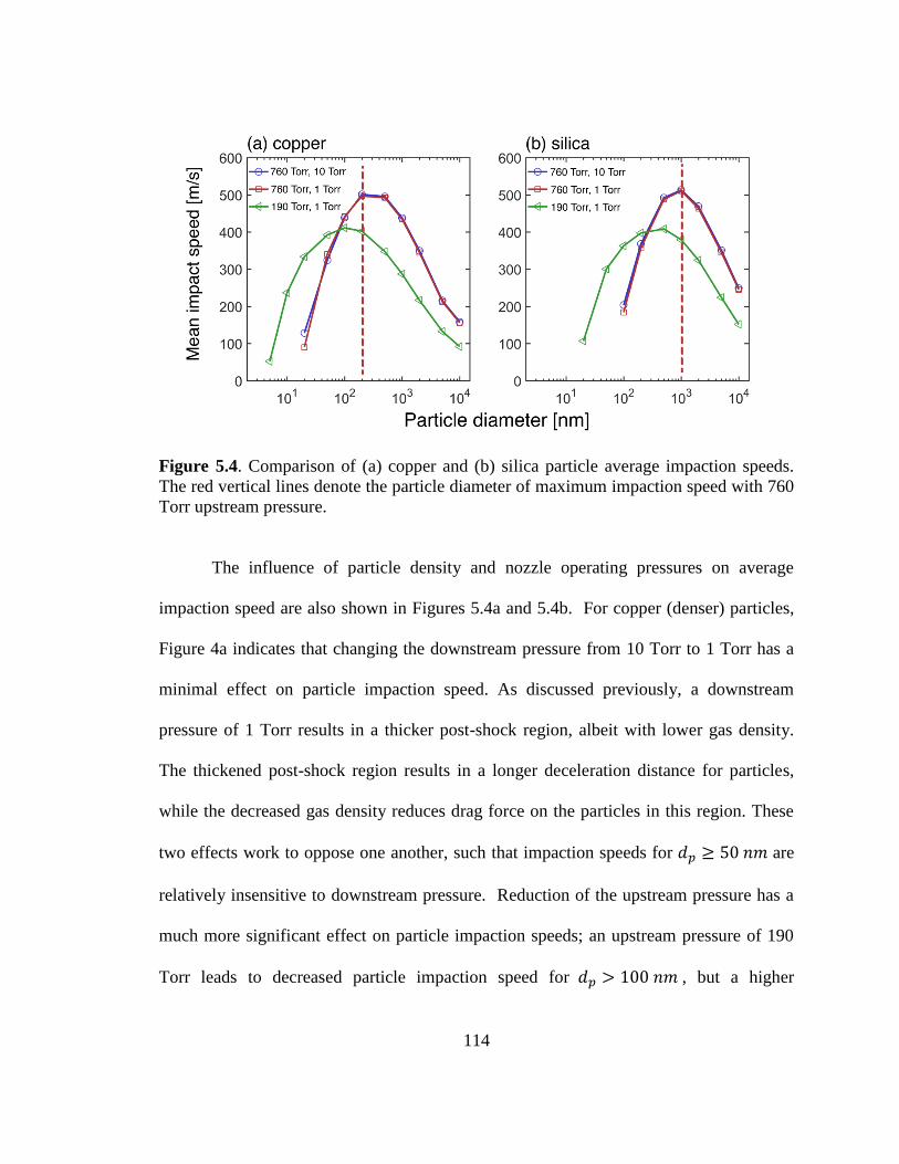
114
Figure 5.4. Comparison of (a) copper and (b) silica particle average impaction speeds.
The red vertical lines denote the particle diameter of maximum impaction speed with 760
Torr upstream pressure.
The influence of particle density and nozzle operating pressures on average
impaction speed are also shown in Figures 5.4a and 5.4b. For copper (denser) particles,
Figure 4a indicates that changing the downstream pressure from 10 Torr to 1 Torr has a
minimal effect on particle impaction speed. As discussed previously, a downstream
pressure of 1 Torr results in a thicker post-shock region, albeit with lower gas density.
The thickened post-shock region results in a longer deceleration distance for particles,
while the decreased gas density reduces drag force on the particles in this region. These
two effects work to oppose one another, such that impaction speeds for 𝑑𝑝 ≥ 50 𝑛𝑚 are
relatively insensitive to downstream pressure. Reduction of the upstream pressure has a
much more significant effect on particle impaction speeds; an upstream pressure of 190
Torr leads to decreased particle impaction speed for 𝑑𝑝 > 100 𝑛𝑚 , but a higher

115
impaction speed 𝑑𝑝 < 100 𝑛𝑚. Supported by the results in Figure 5.2d, lowering the
upstream pressure reduces the pressure in the post shock region, facilitating the
deposition of small particles (𝑑𝑝 < 100 𝑛𝑚) but leads to incomplete acceleration of
larger, more inertial particles in the nozzle. A comparison of Figure 5.4b to Figure 5.4a
indicates that silica particle impaction speed follows the same trend qualitatively as
copper particle impaction speed, but with one noticeable difference. The particle size for
the maximum impaction speed is larger for silica particles (~1𝜇𝑚). Such a difference
arises because silica particles have lower densities, and hence less inertia than copper
particles of the same diameter. Though not shown, for silica, the maximally focused
particle diameter is near 2 𝜇m. Interestingly, the maximally focused particle diameter is
larger than the particle diameter of maximum impaction speed for both materials. It is
presently unclear if this is true in all deposition systems; all converging-diverging AD
systems will display a maximally focused particle diameter and have maximum
impaction speed diameter, though a clear relationship between these two diameters is
likely system specific.
5.3.3 Mass, Momentum and Energy Transfer
5.3.3.1 A Framework for Flux Calculations
With particle size dependent impaction velocities and spatial distributions known,
in this section we develop a framework to analyze the mass, momentum and kinetic
energy fluxes to the substrate for any spatially uniform particle size distribution function
in the upstream flow of the nozzle. The mass flux (𝑀𝐴) at a point A on the substrate,
which is a distance r from the center of the substrate, is given by:
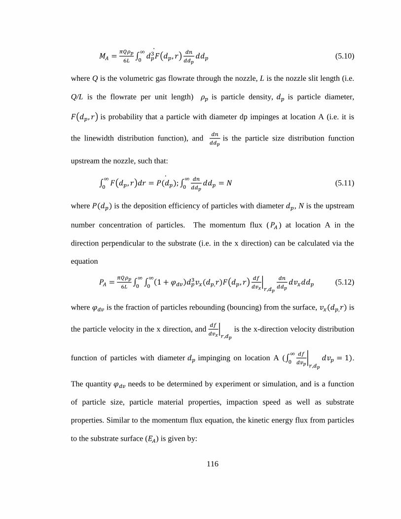
116
𝑀𝐴 =𝜋𝑄𝜌𝑝
6𝐿∫ 𝑑𝑝
3𝐹(𝑑𝑝, 𝑟)𝑑𝑛
𝑑𝑑𝑝𝑑𝑑𝑝
∞
0
(5.10)
where Q is the volumetric gas flowrate through the nozzle, L is the nozzle slit length (i.e.
Q/L is the flowrate per unit length) 𝜌𝑝 is particle density, 𝑑𝑝 is particle diameter,
𝐹(𝑑𝑝, 𝑟) is probability that a particle with diameter dp impinges at location A (i.e. it is
the linewidth distribution function), and 𝑑𝑛
𝑑𝑑𝑝 is the particle size distribution function
upstream the nozzle, such that:
∫ 𝐹(𝑑𝑝, 𝑟)𝑑𝑟∞
0= 𝑃(𝑑𝑝); ∫
𝑑𝑛
𝑑𝑑𝑝𝑑𝑑𝑝
∞
0= 𝑁
(5.11)
where 𝑃(𝑑𝑝) is the deposition efficiency of particles with diameter 𝑑𝑝, N is the upstream
number concentration of particles. The momentum flux (𝑃𝐴 ) at location A in the
direction perpendicular to the substrate (i.e. in the x direction) can be calculated via the
equation
𝑃𝐴 =𝜋𝑄𝜌𝑝
6𝐿∫ ∫ (1 + 𝜑𝑑𝑣)𝑑𝑝
3𝑣𝑥(𝑑𝑝,𝑟)𝐹(𝑑𝑝, 𝑟)𝑑𝑓
𝑑𝑣𝑥|𝑟,𝑑𝑝
𝑑𝑛
𝑑𝑑𝑝𝑑𝑣𝑥𝑑𝑑𝑝
∞
0
∞
0 (5.12)
where 𝜑𝑑𝑣 is the fraction of particles rebounding (bouncing) from the surface, 𝑣𝑥(𝑑𝑝,𝑟) is
the particle velocity in the x direction, and 𝑑𝑓
𝑑𝑣𝑥|𝑟,𝑑𝑝
is the x-direction velocity distribution
function of particles with diameter 𝑑𝑝 impinging on location A (∫𝑑𝑓
𝑑𝑣𝑝|𝑟,𝑑𝑝
𝑑𝑣𝑝∞
0= 1).
The quantity 𝜑𝑑𝑣 needs to be determined by experiment or simulation, and is a function
of particle size, particle material properties, impaction speed as well as substrate
properties. Similar to the momentum flux equation, the kinetic energy flux from particles
to the substrate surface (𝐸𝐴) is given by:
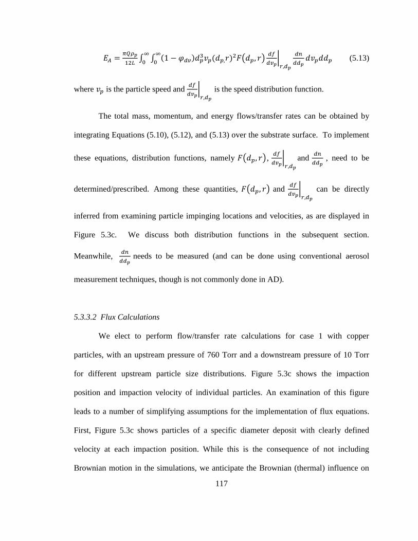
117
𝐸𝐴 =𝜋𝑄𝜌𝑝
12𝐿∫ ∫ (1 − 𝜑𝑑𝑣)𝑑𝑝
3𝑣𝑝(𝑑𝑝,𝑟)2𝐹(𝑑𝑝, 𝑟)
𝑑𝑓
𝑑𝑣𝑝|𝑟,𝑑𝑝
𝑑𝑛
𝑑𝑑𝑝𝑑𝑣𝑝𝑑𝑑𝑝
∞
0
∞
0 (5.13)
where 𝑣𝑝 is the particle speed and 𝑑𝑓
𝑑𝑣𝑝|𝑟,𝑑𝑝
is the speed distribution function.
The total mass, momentum, and energy flows/transfer rates can be obtained by
integrating Equations (5.10), (5.12), and (5.13) over the substrate surface. To implement
these equations, distribution functions, namely 𝐹(𝑑𝑝, 𝑟), 𝑑𝑓
𝑑𝑣𝑝|𝑟,𝑑𝑝
and 𝑑𝑛
𝑑𝑑𝑝 , need to be
determined/prescribed. Among these quantities, 𝐹(𝑑𝑝, 𝑟) and 𝑑𝑓
𝑑𝑣𝑝|𝑟,𝑑𝑝
can be directly
inferred from examining particle impinging locations and velocities, as are displayed in
Figure 5.3c. We discuss both distribution functions in the subsequent section.
Meanwhile, 𝑑𝑛
𝑑𝑑𝑝 needs to be measured (and can be done using conventional aerosol
measurement techniques, though is not commonly done in AD).
5.3.3.2 Flux Calculations
We elect to perform flow/transfer rate calculations for case 1 with copper
particles, with an upstream pressure of 760 Torr and a downstream pressure of 10 Torr
for different upstream particle size distributions. Figure 5.3c shows the impaction
position and impaction velocity of individual particles. An examination of this figure
leads to a number of simplifying assumptions for the implementation of flux equations.
First, Figure 5.3c shows particles of a specific diameter deposit with clearly defined
velocity at each impaction position. While this is the consequence of not including
Brownian motion in the simulations, we anticipate the Brownian (thermal) influence on
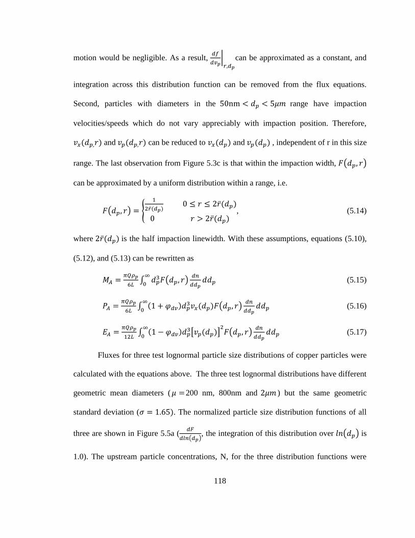
118
motion would be negligible. As a result, 𝑑𝑓
𝑑𝑣𝑝|𝑟,𝑑𝑝
can be approximated as a constant, and
integration across this distribution function can be removed from the flux equations.
Second, particles with diameters in the 50nm < 𝑑𝑝 < 5𝜇𝑚 range have impaction
velocities/speeds which do not vary appreciably with impaction position. Therefore,
𝑣𝑥(𝑑𝑝,𝑟) and 𝑣𝑝(𝑑𝑝,𝑟) can be reduced to 𝑣𝑥(𝑑𝑝) and 𝑣𝑝(𝑑𝑝) , independent of r in this size
range. The last observation from Figure 5.3c is that within the impaction width, 𝐹(𝑑𝑝, 𝑟)
can be approximated by a uniform distribution within a range, i.e.
𝐹(𝑑𝑝, 𝑟) = {
1
2��(𝑑𝑝) 0 ≤ 𝑟 ≤ 2��(𝑑𝑝)
0 𝑟 > 2��(𝑑𝑝) , (5.14)
where 2��(𝑑𝑝) is the half impaction linewidth. With these assumptions, equations (5.10),
(5.12), and (5.13) can be rewritten as
𝑀𝐴 =𝜋𝑄𝜌𝑝
6𝐿∫ 𝑑𝑝
3𝐹(𝑑𝑝, 𝑟)𝑑𝑛
𝑑𝑑𝑝𝑑𝑑𝑝
∞
0 (5.15)
𝑃𝐴 =𝜋𝑄𝜌𝑝
6𝐿∫ (1 + 𝜑𝑑𝑣)𝑑𝑝
3𝑣𝑥(𝑑𝑝)𝐹(𝑑𝑝, 𝑟)𝑑𝑛
𝑑𝑑𝑝𝑑𝑑𝑝
∞
0 (5.16)
𝐸𝐴 =𝜋𝑄𝜌𝑝
12𝐿∫ (1 − 𝜑𝑑𝑣)𝑑𝑝
3[𝑣𝑝(𝑑𝑝)]2𝐹(𝑑𝑝, 𝑟)
𝑑𝑛
𝑑𝑑𝑝𝑑𝑑𝑝
∞
0 (5.17)
Fluxes for three test lognormal particle size distributions of copper particles were
calculated with the equations above. The three test lognormal distributions have different
geometric mean diameters (𝜇 =200 nm, 800nm and 2𝜇𝑚 ) but the same geometric
standard deviation (𝜎 = 1.65). The normalized particle size distribution functions of all
three are shown in Figure 5.5a (𝑑𝐹
𝑑𝑙𝑛(𝑑𝑝), the integration of this distribution over 𝑙𝑛(𝑑𝑝) is
1.0). The upstream particle concentrations, N, for the three distribution functions were
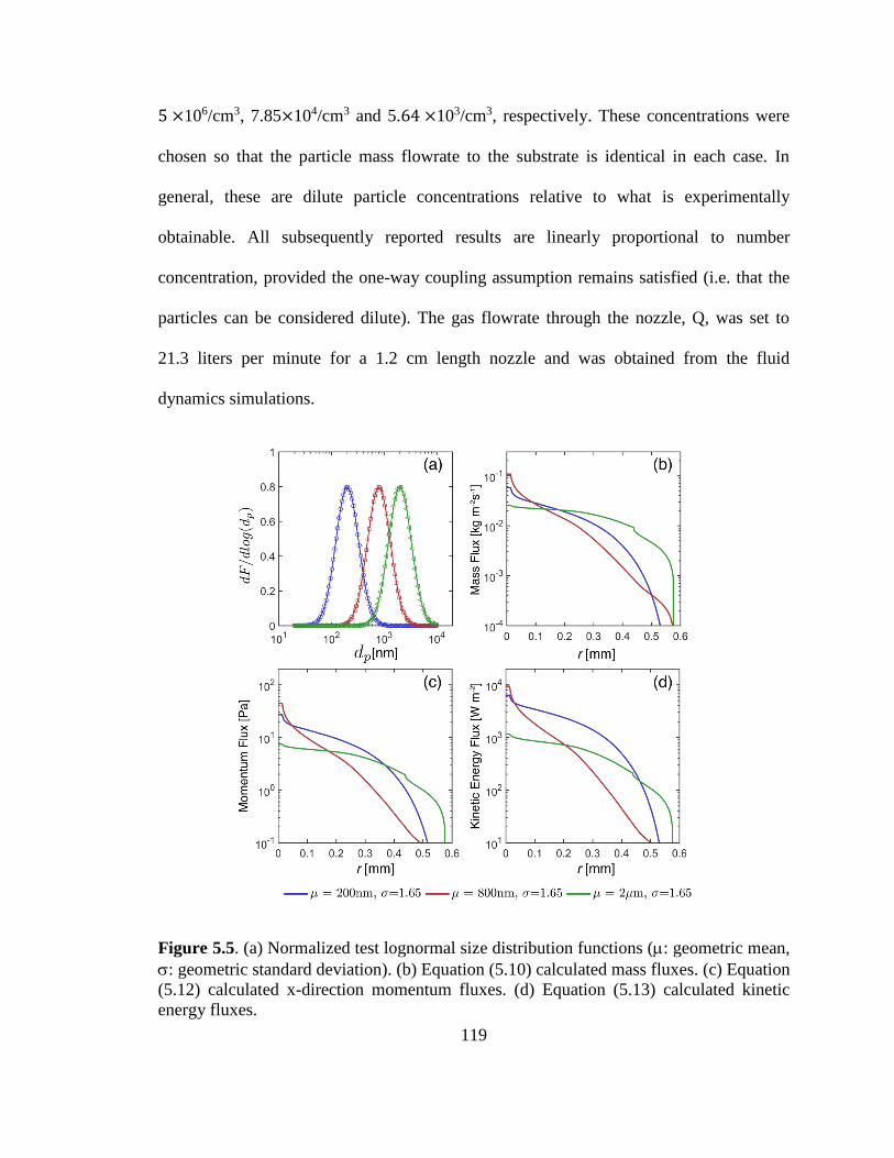
119
5 ×10⁶/cm3, 7.85×10⁴/cm3 and 5.64 ×10³/cm3, respectively. These concentrations were
chosen so that the particle mass flowrate to the substrate is identical in each case. In
general, these are dilute particle concentrations relative to what is experimentally
obtainable. All subsequently reported results are linearly proportional to number
concentration, provided the one-way coupling assumption remains satisfied (i.e. that the
particles can be considered dilute). The gas flowrate through the nozzle, Q, was set to
21.3 liters per minute for a 1.2 cm length nozzle and was obtained from the fluid
dynamics simulations.
Figure 5.5. (a) Normalized test lognormal size distribution functions (: geometric mean,
: geometric standard deviation). (b) Equation (5.10) calculated mass fluxes. (c) Equation
(5.12) calculated x-direction momentum fluxes. (d) Equation (5.13) calculated kinetic
energy fluxes.
120
The mass, x-momentum, and kinetic energy fluxes are plotted as functions of
distance to the substrate center (r) in Figures 5.5b, 5.5c and 5.5d, respectively. The
sudden drop in the 2 mm geometric mean curves near 4.5 mm arises because large
particle deposition within the nozzle (affecting larger particle linewidth distribution
functions). For mass fluxes, passage through the converging-diverging nozzle system has
a clear focusing effect for all three distributions, as the mass flux is an order of magnitude
higher (or more) at the nozzle center. Distribution 2 (𝜇 =800 nm) is most focused, while
distribution 1 (𝜇 =2 𝜇m) is the least focused. This is a direct result of the size-dependent
focusing effect shown in Figure 5.3d. We note that although the geometric mean of
distribution 3 (𝜇 = 2𝜇𝑚) is close to the optimal focusing size (refer to Figure 5.3d), the
particles that take up the majority of particle mass have sizes greater than 2𝜇𝑚; these
particles are not as well focused.
Momentum and kinetic energy fluxes follow the same qualitative trend as the
mass fluxes. However, it is not directly obvious from Figures 5.5c and 5.5d if momentum
and kinetic energy are more focused than mass. To facilitate comparison, the ratio of
mass, momentum and kinetic energy deposited within r < 0.1 mm and total mass,
momentum and kinetic energy transfer rate is calculated for all three distributions (r = 0.1
mm corresponds to an impaction width of 0.2mm, which is the throat width of the
nozzle). The ratios are provided in Table 5.2, together with the total transfer quantities.
For distribution function 1, mass, momentum and kinetic energy have similar ratios,
indicating the particles deposited within r < 0.1 mm do not have higher than average
impaction speed. For distribution functions 2 and 3, kinetic energy and momentum are
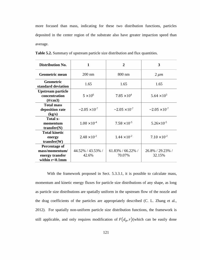
121
more focused than mass, indicating for these two distribution functions, particles
deposited in the center region of the substrate also have greater impaction speed than
average.
Table 5.2. Summary of upstream particle size distribution and flux quantities.
Distribution No. 1 2 3
Geometric mean 200 nm 800 nm 2 𝜇𝑚
Geometric
standard deviation 1.65 1.65 1.65
Upstream particle
concentration
(#/cm3)
5 ×10⁶ 7.85 ×10⁴ 5.64 ×10³
Total mass
deposition rate
(kg/s)
~2.05 ×10⁻⁷ ~2.05 ×10⁻⁷ ~2.05 ×10⁻⁷
Total x-
momentum
transfer(N)
1.00 ×10⁻⁴ 7.58 ×10⁻⁵ 5.26×10⁻⁵
Total kinetic
energy
transfer(W)
2.48 ×10⁻² 1.44 ×10⁻² 7.10 ×10⁻²
Percentage of
mass/momentum/
energy transfer
within r<0.1mm
44.52% / 43.53% /
42.6%
61.83% / 66.22% /
70.07%
26.8% / 29.23% /
32.15%
With the framework proposed in Sect. 5.3.3.1, it is possible to calculate mass,
momentum and kinetic energy fluxes for particle size distributions of any shape, as long
as particle size distributions are spatially uniform in the upstream flow of the nozzle and
the drag coefficients of the particles are appropriately described (C. L. Zhang et al.,
2012). For spatially non-uniform particle size distribution functions, the framework is
still applicable, and only requires modification of 𝐹(𝑑𝑝, 𝑟)(which can be easily done
122
when the spatial particle concentration function is prescribed). Also noteworthy in
Figures 5.5c and 5.5d is that the momentum flux is relatively small (< 100 Pa) while the
kinetic energy flux can be close to 104 W m-2, even for the moderate particle number
concentrations examined (concentrations two orders of magnitude higher are possible
with standard fluidization approaches). This suggests that on average (not necessarily per
particle impact) there is not a high pressure placed on the substrate by particle impaction.
However, translational kinetic energy to thermal kinetic energy conversation can be
extremely high, approaching a magnitude normally observed in convective heat transfer
with phase change (particularly if the particle number exceeds the test concentration by
an order of magnitude or more). Though this would be counteracted by convective
cooling from the gas around the substrate, kinetic to thermal energy transfer may
facilitate particle coalescence upon impact and may be a key reason that AD can yield
dense, non-particulate coatings. We suggest that future studies of the AD process further
investigate kinetic to thermal energy transfer during particle deposition, as energy flux
calculations suggest the rate is high, enhanced by focusing effects, and strongly
dependent and particle size distribution function. Such future investigations will require
more detailed investigation of the one-way coupling assumption, which may breakdown
if a sufficiently high concentration of particles is focused inertially.
5.4 Conclusions
We apply a trajectory calculation approach to examine particle transport in
supersonic aerosol deposition using a converging-diverging nozzle and subsequently
develop approaches to examine mass, momentum, and kinetic energy fluxes due to
123
particle impaction on a substrate. To our knowledge, the latter flux calculations have not
been attempted previously, and in addition the drag correlation applied in trajectory
calculations is itself new, and specifically developed for AD gas conditions. Based upon
this study, we draw the following conclusions.
1. The use of upstream atmospheric pressure in AD, as compared to its high
upstream pressure cold spray counterpart, facilitates the inertial deposition of
submicrometer particles. Further reducing the upstream pressure below
atmospheric pressure enables inertial impaction for progressively smaller
particles, which is also observed in experiments (Holman & Kortshagen, 2010).
However, for a given upstream pressure, decreasing the downstream pressure
beyond a critical value does not drastically influence inertial impaction. This is
due to two counteracting effects; at reduced downstream pressure the pressure
within the post-shock region is reduced, but the size of the post-shock region
increases.
2. Simulations were performed dimensionally, mainly because AD conditions lead
to drastically changing pressure and temperature, and hence selection of reference
variables for non-dimensionalization is rather subjective. Nonetheless, we can
generally conclude that in all supersonic deposition systems (i.e. those with
converging-diverging nozzles and a perpendicular substrate), there is a particle
diameter of maximum impaction velocity; smaller diameter particles are
decelerated in the shock and post-shock region while larger particles are not
accelerated to the gas velocity within the nozzle. The particle diameter of
maximum impaction speed can be adjusted by changing nozzle dimensions
124
(though not studied directly here) as well as by varying upstream pressure and
particle density. In addition, lateral inertial focusing in supersonic AD is
significant and there will exist a particle diameter which is optimally focused (i.e.
of infinitesimal deposition linewidth) in converging-diverging nozzle systems.
Particles smaller than the critically focused diameter are underfocused while
larger particles are overfocused. We suggest that future AD and cold spray
systems be designed with the focused particle diameter in mind; rarely is the
interplay between input particle size distribution function and inertial focusing
considered in these processes.
3. Inertial focusing has significant effect on the particle mass, momentum, and
kinetic energy flux distributions at the substrate surface. Among these, most
interesting is the enhancement in kinetic energy flux distributions along the
centerline of the nozzle; it appears such focusing can lead to kinetic energy fluxes
approaching 104 W m-2 for modest aerosol concentrations (and hence up to 106 W
m-2 for much higher concentration systems). We suggest that future studies of
AD examine kinetic energy to thermal energy transfer for particle upon impact in
light of the finding of highly focused kinetic energy transfer.
125
Chapter 6: Differentiation of Normal and Lung Cancer Cell Lines via
VOC Profiling with Proton Transfer Reaction Time-of-Flight Mass
Spectrometry
Abstract: There is growing interest in utilizing volatile organic compound (VOC)
detection schemes in disease diagnosis and in monitoring cellular metabolism.
However, the extent to which VOC analysis can be used in such applications
remains to be determined. In this study, we employed proton transfer reaction-mass
spectrometry (PTR-MS) to profile VOCs sampled from the headspace of in-vitro
cultured cancerous (A549 and SHP-77) and non-cancerous (BEAS-2B) bronchial
epithelial cell lines. The high resolution (>4000) of the mass spectrometer enabled
ion signal distinction and ion formula identification by exact masses with high
certainty in most instances. Using selected, standardized ion signals, we were able to
partially separate different cell types with unsupervised statistical learning
algorithms, i.e., principal component analysis (PCA) and hierarchical clustering.
Separation and identification of cell types from VOC mass spectra was substantially
improved by using supervised statistical learning algorithms. With multiple subsets
of fewer than ten ions selected by an iterative procedure, 100% training and
prediction accuracies were achievable in a repeated 6-fold cross validation using
linear discriminant analysis (LDA) and support vector machine (SVM), which are
both supervised learning algorithms. These results suggest that high-resolution
PTR-MS coupled with supervised learning algorithm-based analysis is effective for
VOC profiling and cell type identification. Furthermore, we found that with an
126
LDA classifier trained on samples cultivated in a single medium (BEGM), accurate
predictions of cell types cultivated in a second medium (RPMI) are possible,
provided that ion signals have been properly standardized.
6.1 Introduction
There is growing interest in developing diagnostic techniques that depend upon
detection and quantification of biologically emitted, volatile organic compounds (VOCs)
in gaseous mixtures (Banday et al., 2011; Rogers, Benkstein, & Semancik, 2012; Tuzson
et al., 2017; Vergara, Benkstein, Montgomery, & Semancik, 2014), in particular as part
of cancer screening (Haick et al., 2014; Hakim et al., 2012; Konvalina & Haick, 2014;
Schmidt & Podmore, 2015). Such VOC profiling techniques have the potential to
transform the manner in which medical diagnoses are performed; VOC profiling is
generally non-invasive, can be performed in real-time, and with automation VOC
analysis could enable point-of-care diagnosis. However, the extent to which VOC
profiling can be used in cancer diagnostics remains to be determined, and there are
presently no standardized and universally employed methods for VOC profile analysis
(Hakim et al., 2012).
In the absence of standard methodologies, a variety of methods and instruments
have been utilized to assess the potential of VOC profiling, using breath collected from
cancer patients as well as headspace from in vitro cell culture experiments. The
instruments employed include gas chromatography-mass spectrometry (GC-MS)
(Filipiak et al., 2008; Kim, Mulholland, Kukuck, & Pui, 2005; Wojciech et al., 2014),
selected ion flow tube-mass spectrometry (SIFT-MS) (Patrik & David, 2008; D. Smith &
127
Spanel, 2005; Sule-Suso, Pysanenko, Spanel, & Smith, 2009), proton transfer reaction-
mass spectrometry (PTR-MS) (Brunner et al., 2010; Tali et al., 2017; Tali et al., 2016;
Wehinger et al., 2007), along with a variety of nanosensors (Bartolazzi et al., 2010; Di
Natale et al., 2003; Machado et al., 2005; Mazzone et al., 2007; Nakhleh et al., 2017; G.
Peng et al., 2010; Gang Peng, Tisch, Adams, et al., 2009; Gang Peng, Tisch, & Haick,
2009; Rogers et al., 2012). GC-MS measurements provide the highest certainty in terms
of compound identification for VOC profiling. However, this approach requires
preconditioning of samples, and the relatively complex sample preparation and
calibration procedures makes GC-MS unfit for online measurements in a diagnostic
setting. Nanosensors are often rapid, portable, and potentially low cost, but individual
sensors commonly respond to a wide range of VOCs (Röck, Barsan, & Weimar, 2008),
complicating the interpretation of the sensor output (Konvalina & Haick, 2014). In
contrast, SIFT-MS and PTR-MS (Adams & Smith, 1976; Lindinger, Hansel, & Jordan,
1998), which are one-dimensional separation detection techniques, are capable of online
identification and quantification of VOCs. In prior studies using PTR-MS and SIFT-MS
for VOC profiling (Brunner et al., 2010; Patrik & David, 2008; Sule-Suso et al., 2009;
Tali et al., 2017; Tali et al., 2016), only unit mass resolution quadruple mass
spectrometers were employed. Unit mass resolution prohibits clear determination of VOC
atomic composition, leading to ambiguity in terms of the compounds detected and
limiting the information obtained.
Online VOC detection with higher-resolution mass spectrometry would enable
direct, near real-time identification of VOCs, and a more complete description of VOC
profiles to aid in differentiation between samples. By itself, however, even highly

128
comprehensive VOC profiling does not necessarily aid in diagnosis or classification.
Typically, unique ions are not detected in different samples/patients, hence diagnosis or
classification must be based upon subtle differences in signal intensity for multiple
analytes. High-resolution VOC profiles need to be coupled with appropriate data analysis
approaches in order to (1) identify metabolic VOCs (biomarkers) whose concentrations
correlate with cell concentration (in in vitro studies) and disease progression; (2) detect
the presence of different cell populations (i.e., cancerous and non-cancerous cells), or
presence or absence of tumors; and (3) assess the degree to which VOC profiling is
sensitive to environmental conditions or sampling procedures.
To date, VOC profiles, quantified by different means, have been analyzed via a
variety of statistical learning algorithms, including principal component analysis (Barash,
Peled, Hirsch, & Haick, 2009; Chen et al., 2016), linear/quadratic discriminant analysis
(Brunner et al., 2010; Wehinger et al., 2007), logistic regression (Kumar et al., 2015), and
support vector machine (Barash et al., 2012). Though prior work has made use of online
mass spectrometry and statistical learning algorithms in VOC profiling in-vitro and in-
vivo, these algorithms have not been applied to online high-resolution mass spectra. To
directly address this gap, we have developed an approach to analyze VOC profiles
generated by lung epithelial cell cultures (both cancerous, A549 and SHP-77, and non-
cancerous BEAS-2B cells) using PTR-MS with a high-resolution (>4000 for most
analytes) time-of-flight mass spectrometer. Measurements were made in real-time, with
VOCs sampled in a continuous flow system. The resulting high-resolution spectra were
analyzed to identify specific ions that correlate with cell concentration and to distinguish
different cell lines from one another. For cell line identification, we employed both
129
unsupervised and supervised learning algorithms; for the latter we specifically utilized
linear discriminant analysis and support vector machine. Through cross-validations, we
discovered that the supervised learning algorithms enabled cell type identification from
high-resolution VOC profiles using signals from fewer than 10 ions. Additionally, we
found that ions used for classifying cells cultivated in one medium (bronchial epithelial
growth medium; BEGM) can be used to predict cell types cultivated in another medium
(RPMI-1640). Based on these results, we propose that high-resolution PTR-MS can
serve as a robust method for VOC profiling from cell culture headspace, and by extension
in a variety of other biological and environmental systems.
6.2 Experimental Section
6.2.1 Cell Culture Preparation
We cultured cells in a manner enabling direct VOC sampling without the need to
remove them from their growth medium. Human immortalized normal bronchial
epithelial cells, BEAS-2B, and lung squamous cell carcinoma cells, A549 and SHP-77,
were purchased from American Type Culture Collection (ATCC), Manassas, VA USA.
BEAS-2B cells were maintained in bronchial epithelial base medium supplemented with
additives (BEGM) provided by the manufacturer as a kit (cat# CC-3170, Lonza Inc.,
Walkersville, MD USA). A549 and SHP-77 were maintained in RPMI-1640 (ATCC, cat#
30-2001) supplemented with 10% fetal bovine serum (RPMI). To normalize growth
medium conditions, all cells were maintained in either BEGM or RPMI-1640 during
VOC sampling.
130
Prior to VOC sampling in BEGM, cells were seeded and cultured overnight in
their respective growth medium at a total of 107 cells per chamber (n = 42) in Corning
CellSTACK® Culture Chambers (Corning #3268, Fisher Scientific, Pittsburgh, PA USA)
(Figure 6.1), as A549 and SHP-77 cells do not adhere well when seeded in BEGM. We
also performed experiments with 2.5106 (n = 6) and 5106 (n = 6) cells per chamber to
examine the influence of cell concentration on classification, but we found no detectable
difference in the results relative to the chambers with 1107 cells. Cells grown overnight
were then washed twice with pre-warmed phosphate buffered saline (PBS) and cultured
in BEGM for an additional 16 - 18 h. For VOC sampling with the RPMI-1640 medium,
cells were seeded and maintained directly in RPMI-1640 for the same duration without
the washing step. All cells were maintained in a humidified incubator at 37°C, 5% CO2,
and atmospheric pressure prior to and during VOC sampling. For growth medium
controls, chambers containing growth medium (BEGM or RPMI-1640) alone were
maintained and sampled under the same culture conditions.
To enable direct VOC sampling, two ports (¼” swagelokTM ports) were custom-
machined in each CellSTACK® Culture Chamber as shown in Figure 6.1. After
machining, each chamber was resterilized using a vaporized peracetic acid (VPA)
sterilant (Revox Sterilization Solutions, Plymouth, MN USA). Culture chambers were
then repackaged and stored prior to use in cell growth.
6.2.2 Cell Culture Headspace VOC Sampling
A custom-made VOC sampling and PTR-MS introduction system was used for all
experiments (depicted in Figure 6.1). VOCs were sampled from the headspace of cell
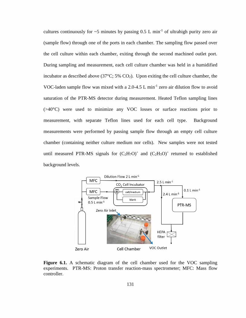
131
cultures continuously for ~5 minutes by passing 0.5 L min-1 of ultrahigh purity zero air
(sample flow) through one of the ports in each chamber. The sampling flow passed over
the cell culture within each chamber, exiting through the second machined outlet port.
During sampling and measurement, each cell culture chamber was held in a humidified
incubator as described above (37°C; 5% CO2). Upon exiting the cell culture chamber, the
VOC-laden sample flow was mixed with a 2.0-4.5 L min-1 zero air dilution flow to avoid
saturation of the PTR-MS detector during measurement. Heated Teflon sampling lines
(>40°C) were used to minimize any VOC losses or surface reactions prior to
measurement, with separate Teflon lines used for each cell type. Background
measurements were performed by passing sample flow through an empty cell culture
chamber (containing neither culture medium nor cells). New samples were not tested
until measured PTR-MS signals for (C2H7O)+ and (C2H5O)+ returned to established
background levels.
Figure 6.1. A schematic diagram of the cell chamber used for the VOC sampling
experiments. PTR-MS: Proton transfer reaction-mass spectrometer; MFC: Mass flow
controller.
132
6.2.3 PTR-MS Operation
VOCs were analyzed with a commercially available PTR-QiTOF (Ionicon
Analytik, GmbH). Instrument settings were optimized to provide high resolution (m/m
~ 4500 for acetone) and sensitivity (700 cps/ppb for acetone). The PTR was operated
with a drift tube pressure of 3.8 mbar, a drift tube temperature of 75°C, E/N of 138 Td,
and an inlet temperature of 75°C. The time-of-flight analyzer was operated over an m/z
range of 0-510 (extraction period 40 μs), with the mass axis calibrated continuously via
addition of a diiodobenzene internal standard. In general, proton transfer reaction is a
relatively soft ionization technique with limited fragmentation, and many VOCs are
detected as the protonated molecular ion at (M+1.008) Th, where M is the molecular
mass of the neutral compound. However, some fragmentation can occur (Yuan et al.,
2017), with the extent dependent upon instrument operating conditions (Baasandorj,
Millet, Hu, Mitroo, & Williams, 2015) (e.g., E/N > 120 Td) and type of VOC (e.g.,
alcohols). Mass axis calibration, transmission correction, and peak fitting and integration
were performed with PTR-MS VIEWER 3.2.5 post processing software, using a
dedicated peak table based on detected peaks over the observed m/z range. Subsequent
data processing was performed using a custom set of R routines (www.R-project.org).
6.3 Data Analysis
Both unsupervised and supervised learning algorithms were employed in
analyzing PTR-MS data in order to assess the relative value of these techniques in VOC
133
profiling with exact mass measurements. We first describe how mass spectrometer signal
intensities were standardized, followed by a description of each employed method.
6.3.1 Cell Type Classification
To determine whether VOC profiling can be used as a robust diagnostic method,
we applied three statistical learning algorithms: Principal component analysis (PCA),
linear discriminant analysis (LDA), and support vector machine (SVM). PCA is an
unsupervised algorithm while the LDA and SVM are supervised learning algorithms.
PCA projects the data onto new dimensions to maximize variance, without taking data
categories (cell types, in our case) into account. LDA assigns a sample to a type that has
the highest posterior probability, assuming different types are normally distributed and
have the same covariance matrix. SVM is a maximum margin classifier that separates
different sample types by a hyperplane in a (p+1)-dimensional space, where p is the
number of features (standardized ion signals, in our case). SVM is readily extendable to
the generation of non-linear separation boundaries via data transformation with non-
linear kernel functions. All three algorithms were implemented with the Python machine
learning package scikit-learn (Pedregosa et al., 2011).
The number of distinct peaks detected by high-resolution PTR-MS for our
samples was more than 600, far exceeding the number of independent measurements (18
samples for each cell type). Using all detected peaks in cell classification would likely
lead to overfitting (Ziegel, 2003) in training the statistical learning algorithms. We thus
employed a procedure to select ions that can best classify and predict cell types.
Specifically, we first selected the 100 most abundant ions in terms of average signals
134
(after averaging over all samples), as higher signal ions are less affected by random
measurement error, and the average signal intensity for ions other than the selected 100
are all below 0.7 counts per second. We next applied a Kruskal-Wallis test to the
standardized signals of the individual ions and retained ions that give a p-value < 0.005
(which indicates there are likely multiple signal intensity distributions present, and the
ion in question may thus be a good predictor of sample type). With the resulting ions, we
then found the optimum combination of k ion signals that yields the highest sample type
prediction accuracy in 6-fold cross validation. We selected 6-fold for the convenience of
data splitting. To mitigate the error introduced by specific fold divisions, we repeated the
cross validation 10 times and obtained an average prediction accuracy, each time using a
different, randomized fold division. The value of k ranges from 1 to the number of ions
identified by the Kruskal-Wallis test. We iterated through all combinations of k ions to
ensure identification of the optimum combination for classification.
6.3.2 Inter-medium Comparison
To compare VOC profiles for cells grown in different media, seven measurements
were performed with cells grown in RPMI (with one measurement for the medium alone,
and two measurements for each cell line). Because the number of measurements for cells
grown in RPMI was limited, we applied the following method to verify that the statistical
learning classifiers built for cell lines grown in BEGM could also be applied to cell lines
grown in RPMI. First, we applied Equation (6.1) to standardize ions signals from cell
lines grown in RPMI. In doing so, only the differences between different cell lines were
preserved, while information regarding absolute VOC concentration was discarded.

135
Second, we built an LDA classifier based on cell lines grown in BEGM using ions
identified by the aforementioned selection procedure. Third, we applied this classifier to
cell lines grown in RPMI to calculate prediction accuracy for the cell lines grown in
RPMI, as well as to visualize where each PTR-MS measurement for RPMI-grown cells
was located in the LDA-transformed coordinates.
6.4 Results and Discussion
6.4.1 PTR-MS Raw Spectra
Figure 6.2. Representative PTR-MS spectra for BEAS-2B (red) and A549 (black) cell
lines. (a) 0-350 Th range mass spectrum. (b) 54-81 Th range mass spectrum. (c)
Separation of C2H3O+ (measured m/z = 43.018) from C3H7
+ (measured m/z = 43.053). (d)
136
Separation of CO2H+ (measured m/z = 44.997) from C2H5O
+ (measured m/z = 45.034).
(e) Ion signal of C5H9+ (major peak, measured m/z = 69.070).
To illustrate differences between VOC profiles from different cell populations,
Figure 6.2 shows the time-averaged representative PTR-MS spectra for one BEAS-2B
sample (red) and one A549 sample (black). Figures 6.2a and 6.2b display the spectra for
m/z ranges of 0-350 Th and 54-81 Th, respectively. From these two figures, it is evident
that (1) VOC concentrations can differ by orders of magnitude, and (2) the ion peaks
detected from both cell populations were identical in exact mass, i.e. biomarkers specific
to only one cell population were not identified from these spectra. Figures 6.2c-6.2e are
amplified versions of the spectra; they highlight ion signal differences from different cell
populations, and further show that the high-resolution PTR-MS separates peaks of the
same nominal mass but disparate exact mass. All three plots show discernable ion signal
differences between the BEAS-2B and A549 samples, although such differences did not
exceed the order of magnitude of the ion signals themselves.
6.4.2 Signal Distribution of Selected Ions
Prior to statistical analysis, we present the standardized concentration
distributions for selected ions produced by cells lines grown in BEGM. These ions were
among those that had the lowest p-values in the Kruskal-Wallis test, and their relatively
low mass-to-charge ratios allowed us to determine their ion formulae with high certainty.
Lower p-values indicate that the detected ion signals were less likely to be sampled from
the same distribution, and therefore are potential ‘biomarkers’ of certain cell lines. The
measured m/z values, tentative ion formulae, and identities of these ions are listed in

137
Table 6.1, along with their p-values. As noted in the “PTR-MS Operation” section,
although PTR-MS employs a soft ionization technique (i.e., proton transfer reaction),
certain species do dissociate/fragment during the ionization process, in some cases
generating akyl chains. For instance, among the ions listed in Table 6.1, m/z = 55.051
corresponds to an ion formula of C4H7+, which could either be a protonated unsaturated
hydrocarbon (e.g., butadiene) or fragment of an aldehyde (Buhr, van Ruth, & Delahunty,
2002; Warneke, de Gouw, Kuster, Goldan, & Fall, 2003) (e.g., butanal). Similarly, m/z =
83.081 corresponds to an ion formula of C6H11+, which could be a protonated unsaturated
hydrocarbon (e.g., hexadiene), or the fragmentation product of an aldehyde or alcohol
(Buhr et al., 2002; Warneke et al., 2003) (e.g., hexanal or hexenol) (Amelynck, Schoon,
Kuppens, Bultinck, & Arijs, 2005; Lee et al., 2006).
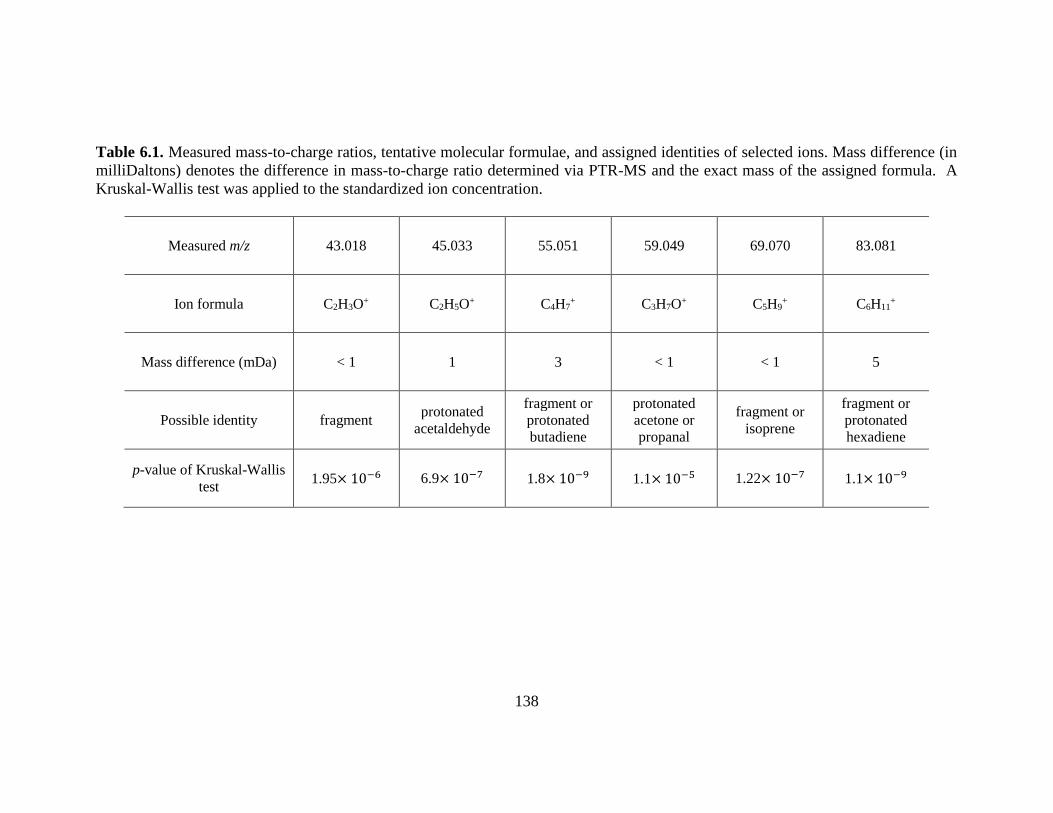
138
Table 6.1. Measured mass-to-charge ratios, tentative molecular formulae, and assigned identities of selected ions. Mass difference (in
milliDaltons) denotes the difference in mass-to-charge ratio determined via PTR-MS and the exact mass of the assigned formula. A
Kruskal-Wallis test was applied to the standardized ion concentration.
Measured m/z 43.018 45.033 55.051 59.049 69.070 83.081
Ion formula C2H3O+ C2H5O+ C4H7+ C3H7O+ C5H9
+ C6H11+
Mass difference (mDa) < 1 1 3 < 1 < 1 5
Possible identity fragment protonated
acetaldehyde
fragment or
protonated
butadiene
protonated
acetone or
propanal
fragment or
isoprene
fragment or
protonated
hexadiene
p-value of Kruskal-Wallis
test 1.95× 10⁻⁶ 6.9× 10⁻⁷ 1.8× 10⁻⁹ 1.1× 10⁻⁵ 1.22× 10⁻⁷ 1.1× 10⁻⁹
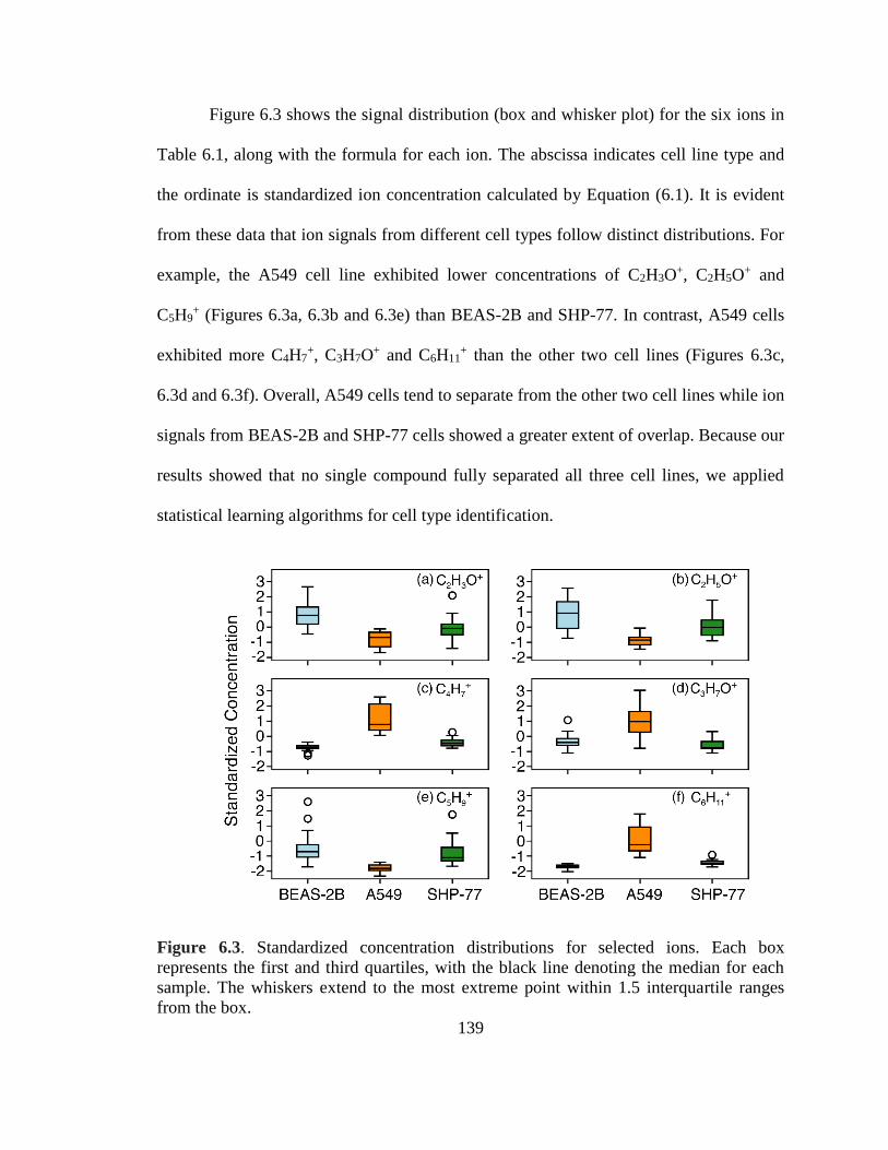
139
Figure 6.3 shows the signal distribution (box and whisker plot) for the six ions in
Table 6.1, along with the formula for each ion. The abscissa indicates cell line type and
the ordinate is standardized ion concentration calculated by Equation (6.1). It is evident
from these data that ion signals from different cell types follow distinct distributions. For
example, the A549 cell line exhibited lower concentrations of C2H3O+, C2H5O
+ and
C5H9+ (Figures 6.3a, 6.3b and 6.3e) than BEAS-2B and SHP-77. In contrast, A549 cells
exhibited more C4H7+, C3H7O
+ and C6H11+ than the other two cell lines (Figures 6.3c,
6.3d and 6.3f). Overall, A549 cells tend to separate from the other two cell lines while ion
signals from BEAS-2B and SHP-77 cells showed a greater extent of overlap. Because our
results showed that no single compound fully separated all three cell lines, we applied
statistical learning algorithms for cell type identification.
Figure 6.3. Standardized concentration distributions for selected ions. Each box
represents the first and third quartiles, with the black line denoting the median for each
sample. The whiskers extend to the most extreme point within 1.5 interquartile ranges
from the box.
140
The ions identified above have been reported previously in VOC profiling of
cancer cell lines (Brunner et al., 2010; Filipiak et al., 2008; D. Smith & Spanel, 2005;
Sponring et al., 2009; Sule-Suso et al., 2009). In particular, m/z = 45.033 likely
corresponds to acetaldehyde, which has been extensively studied in prior in vitro cell
breath studies. The acetaldehyde concentration was previously shown to increase in the
headspace of SK-MES and CALU-I metastatic lung carcinoma cell cultures (D. Smith &
Spanel, 2005; Sule-Suso et al., 2009) and in the headspace of normal lung epithelial
NL20 cell cultures (Sule-Suso et al., 2009), while decreases were observed in 35FL121
Tel+ lung fibroblast cells (Sule-Suso et al., 2009). In contrast, Brunner et al.(Brunner et
al., 2010) reported that acetaldehyde was consumed by A549 and EPLC lung carcinoma
cell lines. Filipiak et al.(Filipiak et al., 2008) and Sponring et al.(Sponring et al., 2009)
also found decreased acetaldehyde concentrations in the headspace of CALU-I and NCI-
H2087 metastatic lung carcinoma cell cultures, respectively. We found that the average
m/z = 45.033 ion concentration decreased in the headspace of the A549 cells compared to
that detected for the BEAS-2B and SHP-77 cell lines. The observed decrease in
acetaldehyde concentration may be due to the increased aldehyde dehydrogenase
(ALDH) enzymatic activity identified in A549 cells (Filipiak et al., 2008).
6.4.3 Statistical Learning Algorithm Classification & Prediction
We used the statistical analysis procedures outlined in the Data Analysis section
to classify and predict different cell types grown in BEGM. By setting a screening
criterion of p < 0.005 in the Kruskal-Wallis test, 19 peaks were selected as candidate
features for statistical learning algorithms. The m/z values of the 19 peaks are provided in
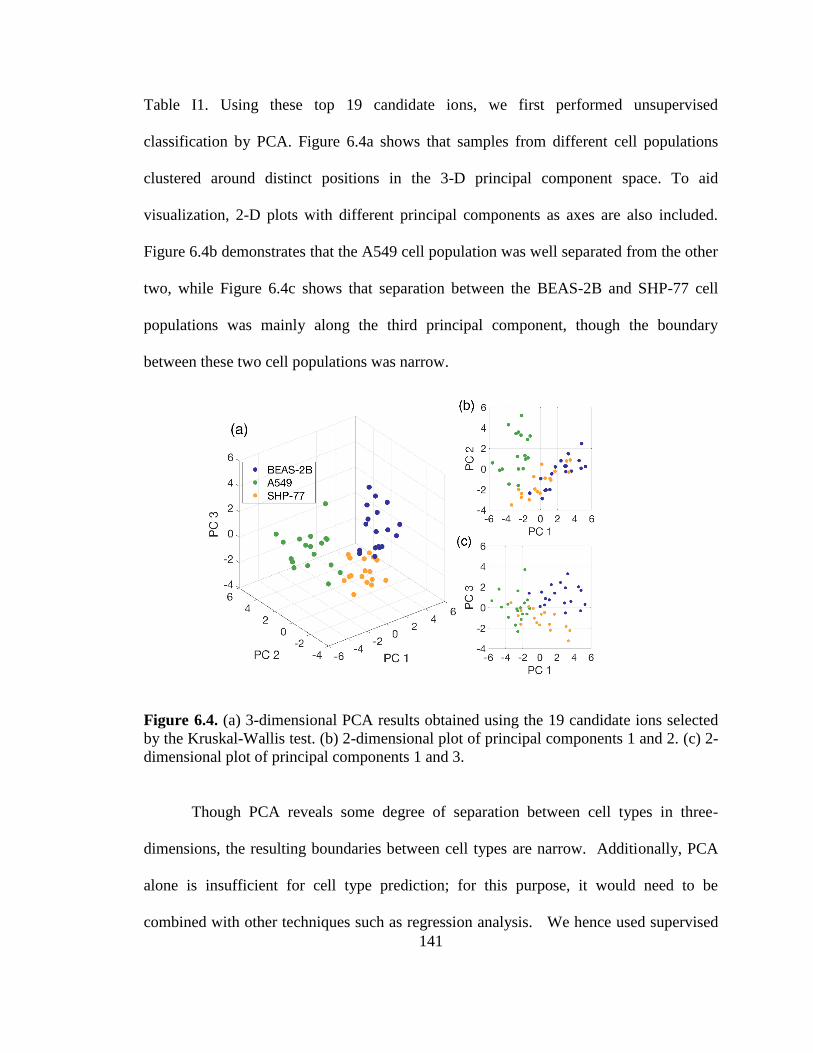
141
Table I1. Using these top 19 candidate ions, we first performed unsupervised
classification by PCA. Figure 6.4a shows that samples from different cell populations
clustered around distinct positions in the 3-D principal component space. To aid
visualization, 2-D plots with different principal components as axes are also included.
Figure 6.4b demonstrates that the A549 cell population was well separated from the other
two, while Figure 6.4c shows that separation between the BEAS-2B and SHP-77 cell
populations was mainly along the third principal component, though the boundary
between these two cell populations was narrow.
Figure 6.4. (a) 3-dimensional PCA results obtained using the 19 candidate ions selected
by the Kruskal-Wallis test. (b) 2-dimensional plot of principal components 1 and 2. (c) 2-
dimensional plot of principal components 1 and 3.
Though PCA reveals some degree of separation between cell types in three-
dimensions, the resulting boundaries between cell types are narrow. Additionally, PCA
alone is insufficient for cell type prediction; for this purpose, it would need to be
combined with other techniques such as regression analysis. We hence used supervised

142
machine learning algorithms (LDA and SVM) to more definitively classify and predict
the cell types using the top 19 candidate ions. The relatively small number of candidates
enabled us to use an iterative method to find the best subset of ions for predicting cell
type with high accuracy. The prediction accuracy is calculated by repeated 6-fold cross
validation. Results from the subset selection are shown in Figure 6.5 for both LDA and
SVM. The abscissa is the number of ions in the subset (k), and the ordinate is the highest
prediction accuracy obtained among all combinations of k ions. For example, if 5 peaks
are chosen to predict the cell type, a total number of 𝐶519 = 11628 ion combinations
exist. Figure 6.5a shows that the highest prediction accuracy achieved by LDA among the
11628 combinations (at k = 5) is 98.1%, while Figure 6.5b shows that the highest
prediction accuracy achieved by SVM is 98.3%. We note that for SVM, a grid search was
performed for the regularization parameter 𝜆 in the range 𝜆 ∈ [0.5, 3]. Results were not
sensitive to the value of 𝜆 within this range and Figure 6.5b shows the result for 𝜆=1.5.
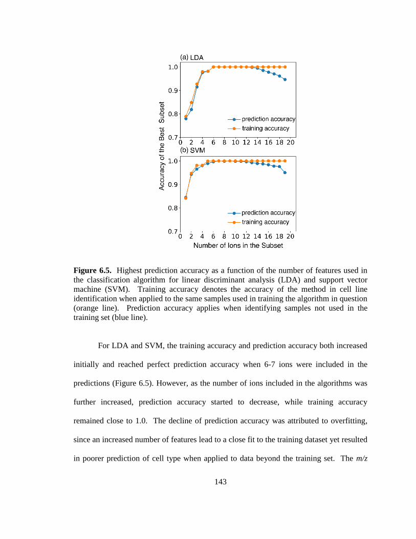
143
Figure 6.5. Highest prediction accuracy as a function of the number of features used in
the classification algorithm for linear discriminant analysis (LDA) and support vector
machine (SVM). Training accuracy denotes the accuracy of the method in cell line
identification when applied to the same samples used in training the algorithm in question
(orange line). Prediction accuracy applies when identifying samples not used in the
training set (blue line).
For LDA and SVM, the training accuracy and prediction accuracy both increased
initially and reached perfect prediction accuracy when 6-7 ions were included in the
predictions (Figure 6.5). However, as the number of ions included in the algorithms was
further increased, prediction accuracy started to decrease, while training accuracy
remained close to 1.0. The decline of prediction accuracy was attributed to overfitting,
since an increased number of features lead to a close fit to the training dataset yet resulted
in poorer prediction of cell type when applied to data beyond the training set. The m/z

144
values for ions in the best subset for k = 1-5, along with their training and prediction
accuracies, are shown in Table 6.2. We note that the ‘best subset’ of ions is not
necessarily unique, i.e. there can be multiple subsets containing k ions that give the same
or nearly the same prediction accuracies. As a result, the subset presented in Table 6.2
should be regarded as representative of a number of ideal subsets. More comprehensive
results for k = 6~10 are included in Table I2 in Appendix I. It is also important to note
that the results presented in Figure 6.5 are subject to data availability, i.e. a larger dataset
typically enables the effective use of more features without overfitting.

145
Table 6.2. A summary of the highest-level prediction accuracy sets using both linear discriminant analysis and support vector
machine, for k = 1-5.
L
DA
k m/z Prediction Accuracy Training Accuracy
1 83.081 0.780 0.789
2 55.052,149.103 0.819 0.849
3 55.052,70.073,99.080 0.915 0.927
4 70.073,71.050,83.081,149.103 0.976 0.980
5 69.070,70.073,71.050,83.081,149.103 0.981 0.981
SV
M
k m/z Prediction Accuracy Training Accuracy
1 83.081 0.828 0.837
2 55.052,149.103 0.946 0.948
3 55.052,71.050,149.103 0.970 0.980
4 31.018,71.050,83.081,149.103 0.980 0.981
5 43.018,55.052,70.073,71.050,179.106 0.983 0.996
146
Importantly, we found that (1) signal intensity measurements for as few as five
VOC-derived ions allowed identification of the cancer cell lines with high accuracy
(>95%), and (2) multiple subsets in this k-range (k = 1-19) were successful in achieving
high-accuracy prediction. These subsets contain multiple features (standardized ion
signals), yet do not include all features (suppressing overfitting). The data analysis
procedure (Kruskal-Wallis test followed by subset selection) is general and can be
applicable to similar problems. For example, the technique can be applied to non-mass
spectrometric data, or for improved classification by mass spectrometry in other
biological/environmental systems (e.g., bacterial identification).(Hamid et al., 2014)
More advanced data processing techniques, such as quadratic discriminant analysis
(Wehinger et al., 2007) and non-linear SVM (Ziegel, 2003) can be used depending on the
complexity of the problem and data availability, though we find LDA and linear SVM
adequate for the present study.
6.4.4 Predicting Cell Type Cultivated in a Distinct Medium (RPMI)
Concentrations of VOCs sampled from cell cultures can certainly be influenced
by medium composition and growth conditions due to changes in metabolic pathways
(Tali et al., 2017). To determine whether the statistical learning classifiers built for cells
grown in one medium can be applied to cells grown in a second medium for cell type
classification, we used 12 ions to build an LDA classifier that was trained on the data
from cells cultured in BEGM growth medium. These ions (denoted by ‘*’ in Table I1)
were chosen by the same subset selection procedure as above and achieved 100%
prediction accuracy in cross validation for cell lines grown in BEGM. We then applied

147
this classifier to the 6 cell culture samples (two of each cell line) grown in RPMI. Prior to
classification, we standardized the ion signals of the 6 samples grown in RPMI using
Equation (6.1).
We found that cell types grown in both BEGM and RPMI medium are well-
separated, and the prediction accuracy is 100% (6/6) for cell lines grown in RPMI. Figure
6.6 shows the location of each cell type in the transformed coordinates by LDA.
Compared to the PCA results shown in Figure 6.4, separation of different cell types was
significantly improved; the boundary areas between cell types are comparable in size to
the areas spanned by individual cell type data in Figure 6.6. Figure 6.6 also suggests that
by using properly standardized data analysis procedures with exact mass PTR-MS, it is
possible to build statistical learning classifiers that successfully predict cell types across
distinct mediums. We note that the use of standardized data (e.g., via Equation (6.1)) is
necessary to achieve cross-medium classification since classification using
unstandardized data was unsuccessful (data not shown). This issue arises because signals
of the same ion from different media can differ significantly (even by orders of
magnitude). For example, the m/z = 45.035 (likely protonated acetaldehyde) ion signals
obtained from the BEGM medium are ~104 counts per second, versus ~102 counts per
second for RPMI. Despite such differences in ion signal intensity, the standardization
process (population averaging) converts ion signals to the same order of magnitude while
preserving differences between cell lines, thus allowing the LDA classifier to be applied
across cells grown under different conditions.

148
Figure 6.6. The positions of all samples on LDA transformed coordinates. The LDA is
trained on 54 cell culture samples grown in BEGM, with 18 samples from each cell line.
Twelve ions, selected by the subset selection procedure, are used as features for LDA.
The trained LDA is then applied to standardized signals from 6 cell cultures grown in
RPMI.
6.5 Conclusions
We performed online VOC profiling using proton transfer reaction time-of-flight
mass spectrometry for in vitro cultured cancerous (A549 and SHP-77) and non-cancerous
(BEAS-2B) cell lines. Based upon this study, we draw the following conclusions:
1. Compared to previous studies using PTR-MS, the high resolution of the
instrument used in this study allowed us to determine the exact atomic
composition of certain detected ions, greatly reducing the uncertainties in peak
assignment.
149
2. Standardized ion signals from different cell populations followed distinct
distributions. Statistical learning algorithms, both unsupervised (PCA and 2D-
hierarchical clustering) and supervised (LDA and SVM), were applied to the
standardized ion signals. Although PCA and hierarchical clustering enabled some
degree of cell type separation, we were able to predict cell types with higher
accuracy and confidence using LDA and SVM. An iterative selection method
was employed to identify the best ion subsets for cell type classification. With
multiple selected subsets, 100% prediction accuracy was achieved in repeated 6-
fold cross validation.
3. Using an LDA classifier built for cells grown in BEGM, we were able to identify
cell types grown in RPMI, despite the differences between VOC absolute
concentrations from the two different growth conditions. Ion signal
standardization that preserves differences between cell lines was required for such
cross-media classification. To examine the limitations of this approach, more
experiments with other cell lines and different growth conditions are needed.
4. The method presented for this study (VOC profiling by high resolution PTR-MS
followed by ion signal standardization, Kruskal-Wallis test, and subset selection)
can be incorporated into a framework for fast classification of in vitro cultured
cell lines. This approach could be useful for the development of non-invasive
methods for cancer diagnosis from human breath.
150
Chapter 7: Conclusions
The studies performed in this thesis aimed to further our understanding of particle
formation, growth, and transport. Additionally, volatile organic compound profiling was
performed to explore the possibility of cell type classification and prediction. These
studies collectively lead to the following conclusions:
First, by non-dimensionalizing the general dynamic equation, solutions were
obtained for a constant reaction rate system with a discrete-sectional model. The
solutions were independent of the production rate of the condensing species; instead, they
depend on a set of dimensionless parameters that characterizes evaporation, particle loss
processes, dilution, and acid-base reaction. It was demonstrated that for a single species
system, particle nucleation approaches the collision-controlled limit as the relevant
dimensionless parameters approach zero. For nucleation involving acid-base reactions,
the collision-controlled limit was reached when the dimensionless base concentration is
sufficiently high. As a result, these parameters provide a guide to determine if a specific
process has a significant effect on particle nucleation and growth. Using the same
framework, the errors of commonly used growth rate calculation methods were
evaluated. It was found that the log-normal distribution function method could lead to an
overestimation of the true particle growth rate by a factor as large as 6. The maximum
overestimation occurs at the collision-controlled limit, at which a maximum number of
particles were produced that lead to significant particle coagulation. It was also shown
that preexisting particles affect the particle nucleation process to a greater extent when
evaporation is non-negligible.
151
Second, tandem DMA-MS measurements of organic vapor sorption to sodium
chloride cluster ions suggest heterogeneous vapor uptake strongly depends on the
structure of the vapor molecules, the cluster ion structure and the cluster ion polarity.
Such measurements were performed systematically in this work for the first time.
Butanol and ethanol showed strong uptake by both positive and negative cluster ions.
MEK sorbs to positively charged cluster ions as well, but only slightly to negatively
charged ions. Toluene showed only slight sorption to cluster ions of both polarities. A
Langmuir model with two parameters, activity coefficient and number of sorption sites,
was fitted to the experimental data to quantitatively infer the number of molecules that
sorbs to the cluster ion surface. These results, along with existing CPC activation data,
indicate heterogeneous vapor uptake process should be examined from a molecular
perspective in future studies. Additionally, in the future design of condensers and
condensational particle counters for size ranges close to 1nm, activation efficiencies
should be examined for a variety of clusters with variable structures.
Third, as to particle transport in a converging-diverging nozzle, fluid dynamics
along with particle trajectory simulations of the aerosol deposition process enabled
detailed calculation of particle impaction speeds as well as mass, momentum and heat
transfer rates to the substrate. By fitting to existing experimental data and simulation data
obtained by direct simulation Monte Carlo (DSMC), a neural network fitting was found
to give a more accurate drag law than previously developed empirical correlations. Using
the new drag law, it was found that there was an optimal particle size that achieves
maximum impaction speed due to presence of the shockwave close to substrate. This
indicates a good control over the depositing particle size distribution can maximize
152
particle impaction speed, facilitating production of compact films. Similarly, particle
trajectory simulations showed that size dependent particle inertial focusing occurs, with
an optimal focusing particle size that produces the smallest deposition linewidth on the
substrate; this effect facilitates mass and energy focusing along the centerline of the
nozzle. Future design of the aerosol deposition apparatus should take into the account the
size dependency of the particle impaction speed and particle focusing.
Finally, cell type classification and prediction were performed with PTR-MS
VOC profiling and selected machine learning algorithms. Though unique biomarkers
specific to cell types were not discovered, VOC concentration differences among cell
types were sufficient for accurate cell type classification and prediction. Using a few
standardized ion signals (6~7) as an input to supervised machine learning algorithms can
lead to near 100% prediction accuracy of cell types. It was also found that the influence
of cell culture medium can be mitigated by proper data standardization; as a result,
machine learning classifier trained with samples cultivated in one medium can be used to
predict cell types cultivated in another medium. The result of this study suggests robust
cell type prediction can be achieved based on VOC measurements by PTR-MS.

153
Bibliography
Abouali, O., & Ahmadi, G. (2005). A model for supersonic and hypersonic impactors for nanoparticles. Journal of Nanoparticle Research, 7(1), 75-88. doi:10.1007/s11051-004-7910-3
Adachi, M., Okuyama, K., Kousaka, Y., & Tanaka, H. (1988). Preparation of gas sensitive film by deposition of ultrafine tin dioxide particles. Journal of Aerosol Science, 19(2), 253-263. doi:10.1016/0021-8502(88)90227-3
Adams, N. G., & Smith, D. (1976). The selected ion flow tube (SIFT); A technique for studying ion-neutral reactions. International Journal of Mass Spectrometry and Ion Physics, 21(3), 349-359. doi:10.1016/0020-7381(76)80133-7
Akedo, J. (2006). Aerosol Deposition of Ceramic Thick Films at Room Temperature: Densification Mechanism of Ceramic Layers. Journal of the American Ceramic Society, 89(6), 1834-1839. doi:10.1111/j.1551-2916.2006.01030.x
Akedo, J. (2008). Room Temperature Impact Consolidation (RTIC) of Fine Ceramic Powder by Aerosol Deposition Method and Applications to Microdevices. Journal of Thermal Spray Technology, 17(2), 181-198. doi:10.1007/s11666-008-9163-7
Akedo, J., & Lebedev, M. (1999). Microstructure and Electrical Properties of Lead Zirconate Titanate (Pb(Zr 52 /Ti 48 )O 3 ) Thick Films Deposited by Aerosol Deposition Method. Japanese Journal of Applied Physics, 38(9S), 5397.
Almeida, J., Schobesberger, S., Kürten, A., Ortega, I. K., Kupiainen-Määttä, O., Praplan, A. P., . . . Kirkby, J. (2013). Molecular understanding of sulphuric acid–amine particle nucleation in the atmosphere. Nature, 502, 359. doi:10.1038/nature12663
Amelynck, C., Schoon, N., Kuppens, T., Bultinck, P., & Arijs, E. (2005). A selected ion flow tube study of the reactions of H3O+, NO+ and O2+ with some oxygenated biogenic volatile organic compounds. International Journal of Mass Spectrometry, 247(1), 1-9. doi:10.1016/j.ijms.2005.08.010
Assadi, H., Gärtner, F., Stoltenhoff, T., & Kreye, H. (2003). Bonding mechanism in cold gas spraying. Acta Materialia, 51(15), 4379-4394. doi:10.1016/S1359-6454(03)00274-X
Assadi, H., Schmidt, T., Richter, H., Kliemann, J.-O., Binder, K., Gärtner, F., . . . Kreye, H. (2011). On Parameter Selection in Cold Spraying. Journal of Thermal Spray Technology, 20(6), 1161-1176. doi:10.1007/s11666-011-9662-9
Baasandorj, M., Millet, D., Hu, L., Mitroo, D., & Williams, B. (2015). Measuring acetic and formic acid by proton-transfer-reaction mass spectrometry: sensitivity, humidity dependence, and quantifying interferences. Atmospheric Measurement Techniques, 8(3), 1303-1321.
Bailey, A. B., & Hiatt, J. (1971). Free-flight measurements of sphere drag at subsonic, transonic, supersonic, and hypersonic speeds for continuum, transition, and near-free-molecular flow conditions. Retrieved from
Balabel, A., Hegab, A. M., Nasr, M., & El-Behery, S. M. (2011). Assessment of turbulence modeling for gas flow in two-dimensional convergent–divergent rocket nozzle. Applied Mathematical Modelling, 35(7), 3408-3422. doi:10.1016/j.apm.2011.01.013
Banday, K. M., Pasikanti, K. K., Chan, E. C. Y., Singla, R., Rao, K. V. S., Chauhan, V. S., & Nanda, R. K. (2011). Use of Urine Volatile Organic Compounds To Discriminate Tuberculosis Patients from Healthy Subjects. Analytical Chemistry, 83(14), 5526-5534. doi:10.1021/ac200265g

154
Barash, O., Peled, N., Hirsch, F. R., & Haick, H. (2009). Sniffing the Unique “Odor Print” of Non-Small-Cell Lung Cancer with Gold Nanoparticles. Small, 5(22), 2618-2624. doi:10.1002/smll.200900937
Barash, O., Peled, N., Tisch, U., Bunn, P. A., Hirsch, F. R., & Haick, H. (2012). Classification of lung cancer histology by gold nanoparticle sensors. Nanomedicine : nanotechnology, biology, and medicine, 8(5), 580-589. doi:10.1016/j.nano.2011.10.001
Barsanti, K. C., McMurry, P. H., & Smith, J. N. (2009). The potential contribution of organic salts to new particle growth. Atmos. Chem. Phys., 9(9), 2949-2957. doi:10.5194/acp-9-2949-2009
Bartolazzi, A., Santonico, M., Pennazza, G., Martinelli, E., Paolesse, R., D’Amico, A., & Di Natale, C. (2010). A sensor array and GC study about VOCs and cancer cells. Sensors and Actuators B: Chemical, 146(2), 483-488. doi:10.1016/j.snb.2009.11.046
Boyd, I. D., & Schwartzentruber, T. E. (2017). Nonequilibrium Gas Dynamics and Molecular Simulation: Cambridge University Press.
Brunner, C., Szymczak, W., Höllriegl, V., Mörtl, S., Oelmez, H., Bergner, A., . . . Oeh, U. (2010). Discrimination of cancerous and non-cancerous cell lines by headspace-analysis with PTR-MS. Analytical and Bioanalytical Chemistry, 397(6), 2315-2324. doi:10.1007/s00216-010-3838-x
Buhr, K., van Ruth, S., & Delahunty, C. (2002). Analysis of volatile flavour compounds by Proton Transfer Reaction-Mass Spectrometry: fragmentation patterns and discrimination between isobaric and isomeric compounds. International Journal of Mass Spectrometry, 221(1), 1-7. doi:10.1016/S1387-3806(02)00896-5
Chakrabarty, S., Ferreiro, J. J., Lippe, M., & Signorell, R. (2017). Toluene Cluster Formation in Laval Expansions: Nucleation and Growth. The Journal of Physical Chemistry A, 121(20), 3991-4001. doi:10.1021/acs.jpca.7b03162
Champagne, V. K., Helfritch, D. J., Dinavahi, S. P. G., & Leyman, P. F. (2011). Theoretical and Experimental Particle Velocity in Cold Spray. Journal of Thermal Spray Technology, 20(3), 425-431. doi:10.1007/s11666-010-9530-z
Chan, T. W., & Mozurkewich, M. (2001). Measurement of the coagulation rate constant for sulfuric acid particles as a function of particle size using tandem differential mobility analysis. Journal of Aerosol Science, 32(3), 321-339. doi:10.1016/S0021-8502(00)00081-1
Chen, Y., Zhang, Y., Pan, F., Liu, J., Wang, K., Zhang, C., . . . Cui, D. (2016). Breath Analysis Based on Surface-Enhanced Raman Scattering Sensors Distinguishes Early and Advanced Gastric Cancer Patients from Healthy Persons. ACS Nano, 10(9), 8169-8179. doi:10.1021/acsnano.6b01441
Clark, W. E. (1972). Measurements of aerosols produced by the photochemical oxidation of SO2 in air. (Ph.D.), University of Minnesota, Minneapolis, MN.
Clark, W. E., & Whitby, K. T. (1975). Measurements of Aerosols Produced by the Photochemical Oxidation of SO2 in Air. Journal of Colloid and Interface Science, 51, 477-490.
Crump, J. G., & Seinfeld, J. H. (1981). Turbulent deposition and gravitational sedimentation of an aerosol in a vessel of abritrary shape. J. Aerosol Sci., 12(5), 405-415.
Davies, C. N. (1945). Definitive equations for the fluid resistance of spheres. Proceedings of the Physical Society, 57(4), 259.
Davis, J., Ravindran, P., & Ray, A. K. (1981). Single aerosol particle studies. Advances in Colloid and Interface Sciences, 15, 1-24. doi:10.1016/0001-8686(81)80001-2
155
de Juan, L., & Fernandez de la Mora, J. (1998). Sizing nanoparticles with a focusing impactor: Effect of the collector size. Journal of Aerosol Science, 29(5-6), 589-599.
Di Natale, C., Macagnano, A., Martinelli, E., Paolesse, R., D'Arcangelo, G., Roscioni, C., . . . D'Amico, A. (2003). Lung cancer identification by the analysis of breath by means of an array of non-selective gas sensors. Biosens Bioelectron, 18. doi:10.1016/s0956-5663(03)00086-1
Ding, H., Wang, C., & Wang, G. (2017). Transient conjugate heat transfer in critical flow nozzles. International Journal of Heat and Mass Transfer, 104, 930-942. doi:10.1016/j.ijheatmasstransfer.2016.09.021
Dugourd, P., Hudgins, R. R., & Jarrold, M. F. (1997). High-resolution ion mobility studies of sodium chloride nanocrystals. Chemical Physics Letters, 267(1-2), 186-192. doi:10.1016/s0009-2614(97)00062-6
Fernandez de la Mora, J., Hering, S. V., Rao, N., & McMurry, P. H. (1990). Hypersonic Impaction of Ultrafine Particles. Journal of Aerosol Science, 21(2), 169-187.
Fernández de la Mora, J., Rao, N., & McMurry, P. H. (1990). Inertial impaction of fine particles at moderate reynolds numbers and in the transonic regime with a thin-plate orifice nozzle. Journal of Aerosol Science, 21(7), 889-909. doi:10.1016/0021-8502(90)90160-Y
Filipiak, W., Sponring, A., Mikoviny, T., Ager, C., Schubert, J., Miekisch, W., . . . Troppmair, J. (2008). Release of volatile organic compounds (VOCs) from the lung cancer cell line CALU-1 in vitro. Cancer Cell Int, 8. doi:10.1186/1475-2867-8-17
Fluent, A. (2009). 12.0 User’s guide. Ansys Inc. Friedlander, S. K. (2000). Smoke, dust, and haze : fundamentals of aerosol dynamics (2nd ed..
ed.). New York: New York : Oxford University Press. Fuchs, N. A. (1964). The Mechanics of Aerosols. Oxford: Pergamon Press. Fuchs, N. A., & Sutugin, A. (1971). High dispersed aerosols. In G. M. Hidy & J. R. Brock (Eds.),
Topics in Current Aerosol Research (Part 2) (pp. 1-60). New York: Pergamon. Fuchs, N. A., & Sutugin, A. G. (1971). HIGH-DISPERSED AEROSOLS A2 - HIDY, G.M. In J. R. Brock
(Ed.), Topics in Current Aerosol Research (pp. 1): Pergamon. Gamero-Castano, M., & Fernandez de la Mora, J. (2000). A condensation nucleus counter (CNC)
sensitive to singly charged sub-nanometer particles. Journal of Aerosol Science, 31(7), 757-772. doi:10.1016/s0021-8502(99)00555-8
Gelbard, F., & Seinfeld, J. H. (1979). The general dynamic equation for aerosols. Theory and application to aerosol formation and growth. Journal of Colloid and Interface Science, 68(2), 363-382. doi:10.1016/0021-9797(79)90289-3
Gelbard, F., & Seinfeld, J. H. (1980). Simulation of multicomponent aerosol dynamics. Journal of Colloid and Interface Science, 78(2), 485-501. doi:10.1016/0021-9797(80)90587-1
Goldstein, S. (1938). Modern developments in fluid dynamics: an account of theory and experiment relating to boundary layers, turbulent motion and wakes (Vol. 1): Clarendon Press.
Gopalakrishnan, R., & Hogan Jr., C. J. (2011). Determination of the transition Regime Collision Kernel from Mean First Passage Times. Aerosol Science and Technology, 45(12), 1499-1509. doi:10.1080/02786826.2011.601775
Haick, H., Broza, Y. Y., Mochalski, P., Ruzsanyi, V., & Amann, A. (2014). Assessment, origin, and implementation of breath volatile cancer markers. Chemical Society Reviews, 43(5), 1423-1449. doi:10.1039/c3cs60329f
156
Hakim, M., Broza, Y. Y., Barash, O., Peled, N., Phillips, M., Amann, A., & Haick, H. (2012). Volatile Organic Compounds of Lung Cancer and Possible Biochemical Pathways. Chemical Reviews, 112(11), 5949-5966. doi:10.1021/cr300174a
Hamid, A. M., Jarmusch, A. K., Pirro, V., Pincus, D. H., Clay, B. G., Gervasi, G., & Cooks, R. G. (2014). Rapid Discrimination of Bacteria by Paper Spray Mass Spectrometry. Analytical Chemistry, 86(15), 7500-7507. doi:10.1021/ac501254b
Hanft, D., Exner, J., Schubert, M., Stocker, T., Fuierer, P., & Moos, R. (2015). An Overview of the Aerosol Deposition Method: Process Fundamentals and New Trends in Materials Applications. Journal of Ceramic Science and Technology, 6(3), 147-181. doi:10.4416/jcst2015-00018
Haynes, B. S., & Wagner, H. G. (1981). Soot formation. Progress in Energy and Combustion Science, 7(4), 229-273. doi:10.1016/0360-1285(81)90001-0
Heisler, S. L., & Friedlander, S. K. (1977). Gas-to-particle conversion in photochemical smog: Aerosol growth laws and mechanisms for organics. Atmospheric Environment (1967), 11(2), 157-168. doi:10.1016/0004-6981(77)90220-7
Henderson, C. B. (1976). Drag Coefficients of Spheres in Continuum and Rarefied Flows. AIAA Journal, 14(6), 707-708. doi:10.2514/3.61409
Hodshire, A. L., Lawler, M. J., Zhao, J., Ortega, J., Jen, C., Yli-Juuti, T., . . . Pierce, J. R. (2016). Multiple new-particle growth pathways observed at the US DOE Southern Great Plains field site. Atmos. Chem. Phys., 16(14), 9321-9348. doi:10.5194/acp-16-9321-2016
Hogan, C. J., & Fernandez de la Mora, J. (2009). Tandem ion mobility-mass spectrometry (IMS-MS) study of ion evaporation from ionic liquid-acetonitrile nanodrops. Physical Chemistry Chemical Physics, 11(36), 8079-8090. doi:Doi 10.1039/B904022f
Hogan, C. J., & Fernandez de la Mora, J. (2010). Ion-Pair Evaporation from Ionic Liquid Clusters. Journal of the American Society for Mass Spectrometry, 21(8), 1382-1386. doi:DOI 10.1016/j.jasms.2010.03.044
Holman, Z. C., & Kortshagen, U. R. (2010). A flexible method for depositing dense nanocrystal thin films: impaction of germanium nanocrystals. Nanotechnology, 21(33), 335302.
Huang, C., Nichols, W. T., O’Brien, D. T., Becker, M. F., Kovar, D., & Keto, J. W. (2007). Supersonic jet deposition of silver nanoparticle aerosols: Correlations of impact conditions and film morphologies. Journal of Applied Physics, 101(6), 064902. doi:10.1063/1.2710304
Huang, G., Gu, D., Li, X., Xing, L., & Wang, H. (2014). Numerical simulation on syphonage effect of laval nozzle for low pressure cold spray system. Journal of Materials Processing Technology, 214(11), 2497-2504. doi:10.1016/j.jmatprotec.2014.05.014
Iida, K., Stolzenburg, M. R., & McMurry, P. H. (2009). Effect of working fluid on sub-2 nm particle detection with a laminar flow ultrafine condensation particle counter. Aerosol Science and Technology, 43, 81-96.
Iida, K., Stolzenburg, M. R., McMurry, P. H., Smith, J. N., Quant, F. R., Oberreit, D. R., . . . Hering, S. V. (2008). An ultrafine, water-based condensation particle counter and its evaluation under field conditions. Aerosol Science and Technology, 42(10), 862-871. doi:10.1080/02786820802339579
Jayne, J. T., Leard, D. C., Zhang, X., Davidovits, P., Smith, K. A., Kolb, C. E., & Worsnop, D. R. (2000). Development of an Aerosol Mass Spectrometer for Size and Composition Analysis of Submicron Particles. Aerosol Science and Technology, 33(1-2), 49-70. doi:10.1080/027868200410840
157
Jen, C., McMurry, P. H., & Hanson, D. R. (2014). Stabilization of Sulfuric Acid Dimers by Ammonia, Methylamine, Dimethylamine, and Trimethylamine. Journal of geophysical research, 119, 7502-7514. doi:10.1002/2014JD021592
Jeon, S., Oberreit, D. R., Van Schooneveld, G., Gao, Z., Bischof, J. C., Haynes, C. L., & Hogan, C. J. (2016). Ion-Mobility-Based Quantification of Surface-Coating-Dependent Binding of Serum Albumin to Superparamagnetic Iron Oxide Nanoparticles. ACS Applied Materials & Interfaces, 8(37), 24482-24490. doi:10.1021/acsami.6b09070
Jeon, S., Oberreit, D. R., Van Schooneveld, G., & Hogan, C. J. (2016). Liquid Nebulization-Ion Mobility Spectrometry Based Quantification of Nanoparticle-Protein Conjugate Formation. Analytical Chemistry, 88, 7667–7674.
Johnson, S. D., Schwer, D., Park, D.-S., Park, Y.-S., & Gorzkowski, E. P. (2017). Deposition efficiency of barium hexaferrite by aerosol deposition. Surface and Coatings Technology, 332(Supplement C), 542-549. doi:10.1016/j.surfcoat.2017.06.085
Jun, A., & Maxim, L. (2002). Powder Preparation in Aerosol Deposition Method for Lead Zirconate Titanate Thick Films. Japanese Journal of Applied Physics, 41(11S), 6980.
Kangasluoma, J., Attoui, M., Korhonen, F., Ahonen, L., Siivola, E., & Petaja, T. (2016). Characterization of a Herrmann-type high-resolution differential mobility analyzer. Aerosol Science and Technology, 50(3), 222-229. doi:10.1080/02786826.2016.1142065
Kangasluoma, J., Samodurov, A., Attoui, M., Franchin, A., Junninen, H., Korhonen, F., . . . Kulmala, M. (2016). Heterogeneous Nucleation onto Ions and Neutralized Ions: Insights into Sign-Preference. Journal of Physical Chemistry C, 120(13), 7444-7450. doi:10.1021/acs.jpcc.6b01779
Katanoda, H., Fukuhara, M., & Iino, N. (2007). Numerical Study of Combination Parameters for Particle Impact Velocity and Temperature in Cold Spray. Journal of Thermal Spray Technology, 16(5), 627-633. doi:10.1007/s11666-007-9087-7
Kerminen, V. M., & Kulmala, M. (2002). Analytical formulae connecting the "real" and the "apparent" nucleation rate and the nuclei number concentration for atmospheric nucleation events. Journal of Aerosol Science, 33(4), 609-622.
Kim, J. H., Mulholland, G. W., Kukuck, S. R., & Pui, D. Y. H. (2005). Slip correction measurements of certified PSL nanoparticles using a nanometer differential mobility analyzer (nano-DMA) for Knudsen number from 0.5 to 83. Journal of Research of the National Institute of Standards and Technology, 110(1), 31-54.
Kirkby, J. (2011). Role of sulphuric acid, ammonia and galactic cosmic rays in atmospheric aerosol nucleation. Nature, 476, 429-433.
Kirkby, J., Duplissy, J., Sengupta, K., Frege, C., Gordon, H., Williamson, C., . . . Curtius, J. (2016). Ion-induced nucleation of pure biogenic particles. Nature. doi:10.1038/nature17953
Koirala, R., Pratsinis, S. E., & Baiker, A. (2016). Synthesis of Catalytic Materials in Flames: Opportunities and Challenges. Chem. Soc. Rev., 45, 3053-3068. doi:10.1039/c5cs00011d
Kontkanen, J., Olenius, T., Lehtipalo, K., Vehkamäki, H., Kulmala, M., & Lehtinen, K. E. J. (2016). Growth of atmospheric clusters involving cluster–cluster collisions: comparison of different growth rate methods. Atmos. Chem. Phys., 16(9), 5545-5560. doi:10.5194/acp-16-5545-2016
Konvalina, G., & Haick, H. (2014). Sensors for Breath Testing: From Nanomaterials to Comprehensive Disease Detection. Accounts of Chemical Research, 47(1), 66-76. doi:10.1021/ar400070m
158
Kuang, C., Chen, M., McMurry, P. H., & Wang, J. (2012). Modification of Laminar Flow Ultrafine Condensation Particle Counters for the Enhanced Detection of 1 nm Condensation Nuclei. Aerosol Science and Technology, 46(3), 309-315. doi:10.1080/02786826.2011.626815
Kuang, C., Chen, M., Zhao, J., Smith, J., McMurry, P. H., & Wang, J. (2012). Size and time-resolved growth rate measurements of 1 to 5 nm freshly formed atmospheric nuclei. Atmos. Chem. Phys., 12(7), 3573-3589. doi:10.5194/acp-12-3573-2012
Kuang, C., McMurry, P. H., McCormick, A. V., & Eisele, F. L. (2008). Dependence of nucleation rates on sulfuric acid vapor concentration in diverse atmospheric locations. Journal of Geophysical Research-Atmospheres, 113(D10), D10209. doi:10.1029/2007JD009253
Kuang, C., Riipinen, I., Sihto, S.-L., Kulmala, M., McCormick, A. V., & McMurry, P. H. (2010). An improved criterion for new particle formation in diverse atmospheric environments. Atmospheric Chemistry and Physics, 10(17), 8469-8480. doi:10.5194/acp-10-8469-2010
Kuang, C., Riipinen, I., Yli-Juuti, T., Kulmala, M., McCormick, A. V., & McMurry, P. H. (2010). An improved criterion for new particle formation in diverse atmospheric environments. Atmospheric Chemistry and Physics, 10, 1-12. doi:10.5194/acp-10-1-2010
Kulmala, M., Kerminen, V. M., Anttila, T., Laaksonen, A., & O'Dowd, C. D. (2004). Organic aerosol formation via sulphate cluster activation. Journal of Geophysical Research-Atmospheres, 109(D4). doi:10.1029/2003jd003961
Kulmala, M., Lehtinen, K. E. J., & Laaksonen, A. (2006). Cluster activation theory as an explanation of the linear dependence between formation rate of 3nm particles and sulphuric acid concentration. Atmos. Chem. Phys., 6(3), 787-793. doi:10.5194/acp-6-787-2006
Kulmala, M., Petäjä, T., Nieminen, T., Sipilä, M., Manninen, H. E., Lehtipalo, K., . . . Kerminen, V.-M. (2012). Measurement of the nucleation of atmospheric aerosol particles. Nature Protocols, 7, 1651. doi:10.1038/nprot.2012.091
Kumar, S., Huang, J., Abbassi-Ghadi, N., Mackenzie, H. A., Veselkov, K. A., Hoare, J. M., . . . Hanna, G. B. (2015). Mass Spectrometric Analysis of Exhaled Breath for the Identification of Volatile Organic Compound Biomarkers in Esophageal and Gastric Adenocarcinoma. Annals of Surgery, 262(6), 981-990. doi:10.1097/sla.0000000000001101
Kurten, A., Jokinen, T., Simon, M., Sipilä, M., Sarnela, N., Junninen, H., . . . Curtius, J. (2014). Neutral molecular cluster formation of sulfuric acid–dimethylamine observed in real time under atmospheric conditions. Proceedings of the National Academy of Sciences, 111(42), 15019-15024. doi:doi/10.1073/pnas.1404853111
Kürten, A., Li, C., Bianchi, F., Curtius, J., Dias, A., Donahue, N. M., . . . McMurry, P. H. (2018). New particle formation in the sulfuric acid–dimethylamine–water system: reevaluation of CLOUD chamber measurements and comparison to an aerosol nucleation and growth model. Atmos. Chem. Phys., 18(2), 845-863. doi:10.5194/acp-18-845-2018
Larriba, C., & Hogan, C. J. (2013). Ion Mobilities in Diatomic Gases: Measurement vs. Prediction with Non-Specular Scattering Models. The Journal of Physical Chemistry A, 117, 3887-3901.
Lee, A., Goldstein Allen, H., Keywood Melita, D., Gao, S., Varutbangkul, V., Bahreini, R., . . . Seinfeld John, H. (2006). Gas-phase products and secondary aerosol yields from the ozonolysis of ten different terpenes. Journal of Geophysical Research: Atmospheres, 111, D07302. doi:10.1029/2005jd006437
159
Lee, M.-W., Park, J.-J., Kim, D.-Y., Yoon, S. S., Kim, H.-Y., James, S. C., . . . Coyle, T. (2011). Numerical Studies on the Effects of Stagnation Pressure and Temperature on Supersonic Flow Characteristics in Cold Spray Applications. Journal of Thermal Spray Technology, 20(5), 1085-1097. doi:10.1007/s11666-011-9641-1
Lee, M. W., Park, J. J., Kim, D. Y., Yoon, S. S., Kim, H. Y., Kim, D. H., . . . Park, D. S. (2011). Optimization of supersonic nozzle flow for titanium dioxide thin-film coating by aerosol deposition. Journal of Aerosol Science, 42(11), 771-780. doi:10.1016/j.jaerosci.2011.07.006
Lehtinen, K. E. J., & Kulmala, M. (2003). A model for particle formation and growth in the atmosphere with molecular resolution in size. Atmos. Chem. Phys., 3(1), 251-257. doi:10.5194/acp-3-251-2003
Lehtinen, K. E. J., Rannik, U., Petaja, T., Kulmala, M., & Hari, P. (2004). Nucleation rate and vapor concentration estimations using a least squares aerosol dynamics method - art. no. D21209. Journal of Geophysical Research-Atmospheres, 109(D21), 21209.
Lehtipalo , K., Leppa , J , Kontkanen , J , Kangasluoma , J , Franchin , A , Wimnner , D , Schobesberger , S , Junninen , H , Petaja , T , Sipila , M , Mikkila , J , Vanhanen , J , Worsnop , D R & Kulmala. (2014). Methods for determining particle size distribution and growth rates between 1 and 3 nm using the Particle Size Magnifier. Boreal Environment Research, 19(no. B), 215-236.
Lehtipalo, K., Rondo, L., Kontkanen, J., Schobesberger, S., Jokinen, T., Sarnela, N., . . . Kulmala, M. (2016). The effect of acid-base clustering and ions on the growth of atmospheric nano-particles. Nature Communications, 7, 11594.
Ligor, T., Ligor, M., Amann, A., Ager, C., Bachler, M., Dzien, A., & Buszewski, B. (2008). The analysis of healthy volunteers' exhaled breath by the use of solid-phase microextraction and GC-MS. J Breath Research, 2. doi:10.1088/1752-7155/2/4/046006
Lindinger, W., Hansel, A., & Jordan, A. (1998). Proton-transfer-reaction mass spectrometry (PTR-MS): on-line monitoring of volatile organic compunds at pptv levels. Chem Soc Rev, 27. doi:10.1039/a827347z
Lindquist, G. J., Pui, D. Y. H., & Hogan Jr, C. J. (2014). Porous particulate film deposition in the transition regime. Journal of Aerosol Science, 74(0), 42-51. doi:10.1016/j.jaerosci.2014.03.007
Liu, P., Ziemann, P. J., Kittelson, D. B., & McMurry, P. H. (1995). Generating Particle Beams of Controlled Dimensions and Divergence: I. Theory of Particle Motion in Aerodynamic Lenses and Nozzle Expansions. Aerosol Science and Technology, 22(3), 293-313. doi:10.1080/02786829408959748
Lushnikov, A. A., & Kulmala, M. (1995). Source-Enhanced Condensation in Monocomponent Disperse Systems. Physical Review E, 52(2), 1658-1668.
Machado, R. F., Laskowski, D., Deffenderfer, O., Burch, T., Zheng, S., Mazzone, P. J., . . . Pyle, J. (2005). Detection of lung cancer by sensor array analyses of exhaled breath. Am J Respir Crit Care Med, 171. doi:10.1164/rccm.200409-1184OC
Macrossan, M. N. (2006). Scaling Parameters for Hypersonic Flow: Correlation of Sphere Drag Data. Paper presented at the 25th International Symposium on Rarefied Gas Dynamics
, St. Petersburg, Russia. Maisser, A., Thomas, J. M., Larriba-Andaluz, C., He, S., & Hogan, C. J. (2015). The Mass-Mobility
Distributions of Ions Produced by a Po-210 Source in Air. Journal of Aerosol Science, 90, 36-50.
160
Mallina, R. V., Wexler, A. S., Rhoads, K. P., & Johnston, M. V. (2000). High Speed Particle Beam Generation: A Dynamic Focusing Mechanism for Selecting Ultrafine Particles. Aerosol Science and Technology, 33(1-2), 87-104. doi:10.1080/027868200410868
Marple, V. A., & Willeke, K. (1976). Impactor Design. Atmospheric Environment, 10, 891-896. Mazzone, P. J., Hammel, J., Dweik, R., Na, J., Czich, C., Laskowski, D., & Mekhail, T. (2007).
Diagnosis of lung cancer by the analysis of exhaled breath with a colorimetric sensor array. Thorax, 62(7), 565-568. doi:10.1136/thx.2006.072892
McGrath, M. J., Olenius, T., Ortega, I. K., Loukonen, V., Paasonen, P., Kurtén, T., . . . Vehkamäki, H. (2012). Atmospheric cluster dynamics code: a flexible method for solution of the birth-death equations. Atmos. Chem. Phys., 12, 2345-2355. doi:10.5194/acp-12-2345-2012
McMurry, P. H. (1980). Photochemical aerosol formation from SO2: A theoretical analysis of smog chamber data. Journal of Colloid and Interface Science, 78(2), 513-527. doi:10.1016/0021-9797(80)90589-5
McMurry, P. H. (1983). New Particle Formation in the Presence of an Aerosol: Rates, Time Scales and sub-0.01 µm Size Distributions. Journal of Colloid and Interface Science, 95(1), 72-80.
McMurry, P. H. (2000). The history of condensation nucleus counters. Aerosol Science and Technology, 33(4), 297-322.
McMurry, P. H., Fink, M. A., Sakurai, H., Stolzenburg, M. R., Mauldin, L., Moore, K., . . . Voisin, D. (2005). A Criterion for New Particle Formation in the Sulfur-Rich Atlanta Atmosphere. Journal of Geophysical Research - Atmospheres, 110, D22S02. doi:10.1029/2005JD005901
McMurry, P. H., & Friedlander, S. K. (1979). New particle formation in the presence of an aerosol. Atmos. Environ., 13, 1635-1651.
McMurry, P. H., & Li, C. (2017). The dynamic behavior of nucleating aerosols in constant reaction rate systems: Dimensional analysis and generic numerical solutions. Aerosol Science and Technology, 51(9), 1057-1070. doi:10.1080/02786826.2017.1331292
McMurry, P. H., & Rader, D. J. (1985). Aerosol wall losses in electrically charged chambers. Aerosol Sci. and Technol., 4, 249-268.
McMurry, P. H., & Wilson, J. C. (1982). Growth laws for the formation of secondary ambient aerosols: Implications for chemical conversion mechanisms. Atmospheric Environment (1967), 16(1), 121-134. doi:10.1016/0004-6981(82)90319-5
Menter, F. R. (1994). Two-equation eddy-viscosity turbulence models for engineering applications. AIAA Journal, 32(8), 1598-1605. doi:10.2514/3.12149
Meyer, N. A., Root, K., Zenobi, R., & Vidal-de-Miguel, G. (2016). Gas-Phase Dopant-Induced Conformational Changes Monitored with Transversal Modulation Ion Mobility Spectrometry. Analytical Chemistry, 88(4), 2033-2040. doi:10.1021/acs.analchem.5b02750
Middha, P., & Wexler, A. S. (2003). Particle Focusing Characteristics of Sonic Jets. Aerosol Science and Technology, 37(11), 907-915. doi:10.1080/02786820300934
Millikan, R. A. (1923). Coefficients of Slip in Gases and the Law of Reflection of Molecules from the Surfaces of Solids and Liquids. Physical Review, 21(3), 217-238.
Muneyasu, S., Tetsuo, T., & Jun, A. (2017). Effect of starting powder morphology on film texture for bismuth layer-structured ferroelectrics prepared by aerosol deposition method. Japanese Journal of Applied Physics, 56(6S1), 06GH02.

161
Nakhleh, M. K., Amal, H., Jeries, R., Broza, Y. Y., Aboud, M., Gharra, A., . . . Haick, H. (2017). Diagnosis and Classification of 17 Diseases from 1404 Subjects via Pattern Analysis of Exhaled Molecules. ACS Nano, 11(1), 112-125. doi:10.1021/acsnano.6b04930
Ning, X.-J., Wang, Q.-S., Ma, Z., & Kim, H.-J. (2010). Numerical Study of In-flight Particle Parameters in Low-Pressure Cold Spray Process. Journal of Thermal Spray Technology, 19(6), 1211-1217. doi:10.1007/s11666-010-9548-2
Oberreit, D., Rawat, V. K., Larriba-Andaluz, C., Ouyang, H., McMurry, P. H., & Jr., C. J. H. (2015). Analysis of heterogeneous water vapor uptake by metal iodide cluster ions via differential mobility analysis-mass spectrometry. The Journal of Chemical Physics, 143(10), 104204. doi:10.1063/1.4930278
Oberreit, D. R., McMurry, P. H., & Hogan, C. J. (2014). Analysis of Heterogeneous Vapor Uptake by Nanoparticles via Differential Mobility Analysis-Drift Tube Ion Mobility Spectrometry (DMA-DTIMS). Phys Chem Chem Phys, 16, 6968-6979.
Oberreit, D. R., Rawat, V. K., Larriba-Andaluz, C., Ouyang, H., McMurry, P. H., & Hogan, C. J. (2015). Analysis of heterogeneous water vapor uptake by metal iodide cluster ions via differential mobility analysis-mass spectrometry. The Journal of Chemical Physics, 143, 104204.
Olenius, T., Riipinen, I., Lehtipalo, K., & Vehkamäki, H. (2014). Growth rates of atmospheric molecular clusters based on appearance times and collision–evaporation fluxes: Growth by monomers. Journal of Aerosol Science, 78, 55-70. doi:10.1016/j.jaerosci.2014.08.008
Ouyang, H., Larriba-Andaluz, C., Oberreit, D. R., & Hogan, C. J. (2013). The Collision Cross Sections of Iodide Salt Cluster Ions in Air via Differential Mobility Analysis-Mass Spectrometry Journal of the American Society for Mass Spectrometry, 24, 1833-1847. doi:10.1007/s13361-013-0724-8
Park, J.-J., Kim, D.-Y., Lee, J.-G., Cha, Y.-H., Swihart, M. T., & Yoon, S. S. (2014). Supersonic aerosol-deposited TiO2 photoelectrodes for photoelectrochemical solar water splitting. RSC Advances, 4(17), 8661-8670. doi:10.1039/c3ra47998f
Park, J.-J., Lee, J.-G., Kim, D.-Y., Lee, J.-H., Yun, J. H., Gwak, J., . . . Yoon, S. S. (2017). Rapid supersonic spraying of Cu(In,Ga)(S,Se)2 nanoparticles to fabricate a solar cell with 5.49% conversion efficiency. Acta Materialia, 123, 44-54. doi:10.1016/j.actamat.2016.10.027
Patrik, Š., & David, S. (2008). Quantification of trace levels of the potential cancer biomarkers formaldehyde, acetaldehyde and propanol in breath by SIFT-MS. Journal of Breath Research, 2(4), 046003.
Patterson, G. N. (1971). Introduction to the kinetic theory of gas flows: University of Toronto Press.
Pedregosa, F., Ga, #235, Varoquaux, l., Gramfort, A., Michel, V., . . . Duchesnay, d. (2011). Scikit-learn: Machine Learning in Python. J. Mach. Learn. Res., 12, 2825-2830.
Peng, G., Hakim, M., Broza, Y. Y., Billan, S., Abdah-Bortnyak, R., Kuten, A., . . . Haick, H. (2010). Detection of lung, breast, colorectal, and prostate cancers from exhaled breath using a single array of nanosensors. British Journal Of Cancer, 103, 542. doi:10.1038/sj.bjc.6605810
Peng, G., Tisch, U., Adams, O., Hakim, M., Shehada, N., Broza, Y. Y., . . . Haick, H. (2009). Diagnosing lung cancer in exhaled breath using gold nanoparticles. Nature Nanotechnology, 4, 669. doi:10.1038/nnano.2009.235

162
Peng, G., Tisch, U., & Haick, H. (2009). Detection of Nonpolar Molecules by Means of Carrier Scattering in Random Networks of Carbon Nanotubes: Toward Diagnosis of Diseases via Breath Samples. Nano Letters, 9(4), 1362-1368. doi:10.1021/nl8030218
Pichelstorfer, L., Stolzenburg, D., Ortega, J., Karl, T., Kokkola, H., Laakso, A., . . . Winkler, P. M. (2017). Resolving nanoparticle growth mechanisms from size- and time-dependent growth rate analysis. Atmos. Chem. Phys. Discuss., 2017, 1-24. doi:10.5194/acp-2017-658
Rao, N. P., & McMurry, P. H. (1989). Nucleation and Growth of Aerosol in Chemically Reacting Systems: A Theoretical Study of the Near-Collision-Controlled Regime. Aerosol Science and Technology, 11(2), 120-132. doi:10.1080/02786828908959305
Rao, N. P., Tymiak, N., Blum, J., Neuman, A., Lee, H. J., Girshick, S. L., . . . Heberlein, J. (1998). Hypersonic plasma particle deposition of nanostructured silicon and silicon carbide. Journal of Aerosol Science, 29(5), 707-720. doi:10.1016/S0021-8502(97)10015-5
Rawat, V. K., Vidal-de-Miguel, G., & Hogan, C. J. (2015). Modeling vapor uptake induced mobility shifts in peptide ions observed with transversal modulation ion mobility spectrometry-mass spectrometry. Analyst, 140(20), 6945-6954. doi:10.1039/c5an00753d
Riccobono, F. (2012). Contribution of sulfuric acid and oxidized organic compounds to particle formation and growth. Atmos. Chem. Phys., 12, 9427-9439.
Riccobono, F. (2014). Oxidation products of biogenic emissions contribute to nucleation of atmospheric particles. Science, 344, 717-721.
Riipinen, I., Sihto, S.-L., Kulmala, M., Arnold, F., Dal Maso, M., Birmili, W., . . . Lehtinen, K. E. J. (2007). Connections between atmospheric sulphuric acid and new particle formation during QUEST III - IV campaigns in Hyytiala and Heidelberg. Atmos. Phys. Chem., 7, 1899–1914.
Riipinen, I., Yli-Juuti, T., Pierce, J. R., Petäjä, T., Worsnop, D. R., Kulmala, M., & Donahue, N. M. (2012). The contribution of organics to atmospheric nanoparticle growth. Nature Geoscience, 5, 453. doi:10.1038/ngeo1499
Röck, F., Barsan, N., & Weimar, U. (2008). Electronic Nose: Current Status and Future Trends. Chemical Reviews, 108(2), 705-725. doi:10.1021/cr068121q
Rogers, P. H., Benkstein, K. D., & Semancik, S. (2012). Machine Learning Applied to Chemical Analysis: Sensing Multiple Biomarkers in Simulated Breath Using a Temperature-Pulsed Electronic-Nose. Analytical Chemistry, 84(22), 9774-9781. doi:10.1021/ac301687j
Rus, J., Moro, D., Sillero, J. A., Royuela, J., Casado, A., Estevez-Molinero, F., & Fernandez de la Mora, J. (2010). IMS–MS studies based on coupling a differential mobility analyzer (DMA) to commercial API–MS systems. International Journal of Mass Spectrometry, 298, 30-40.
Saad, M. A. (1985). Compressible fluid flow. Englewood Cliffs, NJ, Prentice-Hall, Inc., 1985. 570 p. Schmidt, K., & Podmore, I. (2015). Current Challenges in Volatile Organic Compounds Analysis as
Potential Biomarkers of Cancer. Journal of Biomarkers, 2015, 16. doi:10.1155/2015/981458
Seinfeld, J. H., & Pandis, S. N. (2016). Atmospheric Chemistry and Physics: From Air Pollution to Climate Change, 3rd Edition. New York: Wiley Interscience.
Shiraiwa, M., Selzle, K., & Pöschl, U. (2012). Hazardous components and health effects of atmospheric aerosol particles: reactive oxygen species, soot, polycyclic aromatic compounds and allergenic proteins. Free Radical Research, 46(8), 927-939. doi:10.3109/10715762.2012.663084
163
Sihto, S. L., Kulmala, M., Kerminen, V. M., Dal Maso, M., Petaja, T., Riipinen, I., . . . Lehtinen, K. E. J. (2006). Atmospheric sulphuric acid and aerosol formation: implications from atmospheric measurements for nucleation and early growth mechanisms. Atmospheric Chemistry and Physics, 6, 4079-4091.
Singh, N., & Schwartzentruber, T. E. (2017). Aerothermodynamic correlations for high-speed flow. Journal of Fluid Mechanics, 821, 421-439. doi:10.1017/jfm.2017.195
Smith, D., & Spanel, P. (2005). Selected ion flow tube mass spectrometry (SIFT-MS) for on-line trace gas analysis. Mass Spectrometry Reviews, 24. doi:10.1002/mas.20033
Smith, J., Dunn, M., VanReken, T., Iida, K., Stolzenburg, M., McMurry, P., & Huey, L. (2008). Chemical composition of atmospheric nanoparticles formed from nucleation in Tecamac, Mexico: Evidence for an important role for organic species in nanoparticle growth. Geophysical Research Letters, 35(4).
Smith, J. N., Barsanti, K. C., Friedli, H. R., Ehn, M., Kulmala, M., Collins, D. R., . . . McMurry, P. H. (2010). Observations of aminium salts in atmospheric nanoparticles and possible climatic implications. Proceedings of the National Academy of Sciences, 107(15), 6634-6639.
Sponring, A., Filipiak, W., Mikoviny, T., Ager, C., Schubert, J., Miekisch, W., . . . Troppmair, J. (2009). Release of volatile organic compounds from the lung cancer cell line NCI-H2087 in vitro. Anticancer Res, 29.
Stalder, J. R., & Zurick, V. J. (1951). Theoretical aerodynamic characteristics of bodies in a free-molecule-flow field. Retrieved from
Steiner, G., & Reischl, G. P. (2012). The effect of carrier gas contaminants on the charging probability of aerosols under bipolar charging conditions. Journal of Aerosol Science, 54(0), 21-31. doi:10.1016/j.jaerosci.2012.07.008
Stoltenhoff, T., Kreye, H., & Richter, H. J. (2002). An analysis of the cold spray process and its coatings. Journal of Thermal Spray Technology, 11(4), 542-550. doi:10.1361/105996302770348682
Stolzenburg, M. R., & McMurry, P. H. (1991). An Ultrafine Aerosol Condensation Nucleus Counter. Aerosol Science and Technology, 14(1), 48-65.
Stolzenburg, M. R., McMurry, P. H., Sakurai, H., Smith, J. N., Mauldin, R. L., Eisele, F. L., & Clement, C. F. (2005). Growth rates of freshly nucleated atmospheric particles in Atlanta. Journal of Geophysical Research: Atmospheres, 110(D22), n/a-n/a. doi:10.1029/2005JD005935
Strobel, R., & Pratsinis, S. E. (2007). Flame aerosol synthesis of smart nanostructured materials. Journal of Materials Chemistry, 17(45), 4743-4756. doi:10.1039/B711652G
Sule-Suso, J., Pysanenko, A., Spanel, P., & Smith, D. (2009). Quantification of acetaldehyde and carbon dioxide in the headspace of malignant and non-malignant lung cellsin vitro by SIFT-MS. Analyst, 134(12), 2419-2425. doi:10.1039/B916158A
Swihart, M. T., & Girshick, S. L. (1999). Thermochemistry and kinetics of silicon hydride cluster formation during thermal decomposition of silane. J. Phys. Chem., 103B, 64-73.
Tali, F., Jens, H., Ingrid, K., Guy, L., John, C. C., Jose, S. T., . . . Nir, P. (2017). Cancer metabolism: the volatile signature of glycolysis— in vitro model in lung cancer cells. Journal of Breath Research, 11(1), 016008.
Tali, F., Layah, A.-M., Jens, H., John, C. C., Jose, S. T., Naomi Gai, M., . . . Nir, P. (2016). Cancerous glucose metabolism in lung cancer—evidence from exhaled breath analysis. Journal of Breath Research, 10(2), 026012.
164
Thimsen, E., Johnson, M., Zhang, X., Wagner, A. J., Mkhoyan, K. A., Kortshagen, U. R., & Aydil, E. S. (2014). High electron mobility in thin films formed via supersonic impact deposition of nanocrystals synthesized in nonthermal plasmas. Nature Communications, 5, 5822. doi:10.1038/ncomms6822
Thomas, J. M., He, S., Larriba-Andaluz, C., DePalma, J. W., Johnston, M., & Hogan, C. J. (2016). Ion Mobility Spectrometry-Mass Spectrometry Examination of the Structures, Stabilities, and Extents of Hydration of Dimethylamine-Sulfuric Acid Clusters. Physical Chemistry Chemical Physics, DOI: 10.1039/C1036CP03432B. doi:10.1039/c6cp03432b
Trimpin, S., & Clemmer, D. E. (2008). Ion Mobility Spectrometry/Mass Spectrometry Snapshots for Assessing the Molecular Compositions of Complex Polymeric Systems. Analytical Chemistry, 80(23), 9073-9083.
Tröstl, J., Chuang, W. K., Gordon, H., Heinritzi, M., Yan, C., Molteni, U., . . . Baltensperger, U. (2016). The role of low-volatility organic compounds in initial particle growth in the atmosphere. Nature, 533, 527. doi:10.1038/nature18271
Tuzson, B., Jágerská, J., Looser, H., Graf, M., Felder, F., Fill, M., . . . Emmenegger, L. (2017). Highly Selective Volatile Organic Compounds Breath Analysis Using a Broadly-Tunable Vertical-External-Cavity Surface-Emitting Laser. Analytical Chemistry, 89(12), 6377-6383.
Ude, S., & Fernandez de la Mora, J. (2005). Molecular monodisperse mobility and mass standards from electrosprays of tetra-alkyl ammonium halides. Journal of Aerosol Science, 36(10), 1224-1237. doi:10.1016/j.jaerosci.2005.02.009
Vanhanen, J., Mikkila, J., Lehtipalo, K., Sipila, M., Manninen, H. E., Siivola, E., . . . Kulmala, M. (2011). Particle Size Magnifier for Nano-CN Detection. Aerosol Science and Technology, 45(4), 533-542. doi:10.1080/02786826.2010.547889
Vergara, A., Benkstein, K. D., Montgomery, C. B., & Semancik, S. (2014). Demonstration of Fast and Accurate Discrimination and Quantification of Chemically Similar Species Utilizing a Single Cross-Selective Chemiresistor. Analytical Chemistry, 86(14), 6753-6757. doi:10.1021/ac501490k
Verheggen, B., & Mozurkewich, M. (2006). An inverse modeling procedure to determine particle growth and nucleation rates from measured aerosol size distributions. Atmospheric Chemistry and Physics, 6, 2927-2942.
Wang, J., McGraw, R. L., & Kuang, C. (2013). Growth of atmospheric nano-particles by heterogeneous nucleation of organic vapor. Atmos. Chem. Phys., 13(13), 6523-6531. doi:10.5194/acp-13-6523-2013
Wang, X. L., Kruis, F. E., & McMurry, P. H. (2005). Aerodynamic focusing of nanoparticles: I. Guidelines for designing aerodynamic lenses for nanoparticles. Aerosol Science and Technology, 39(7), 611-623.
Warneke, C., de Gouw, J. A., Kuster, W. C., Goldan, P. D., & Fall, R. (2003). Validation of Atmospheric VOC Measurements by Proton-Transfer- Reaction Mass Spectrometry Using a Gas-Chromatographic Preseparation Method. Environmental Science & Technology, 37(11), 2494-2501. doi:10.1021/es026266i
Warren, D. R., & Seinfeld, J. H. (1985). Simulation of Aerosol Size Distribution Evolution in Systems with Simultaneous Nucleation, Condensation, and Coagulation. Aerosol Science and Technology, 4(1), 31-43. doi:10.1080/02786828508959037
Weber, R. J., Marti, J., McMurry, P. H., Eisele, F. L., Tanner, D. J., & Jefferson, A. (1996). Measured atmospheric new particle formation rates: implications for nucleation mechanisms. Chem. Eng. Comm., 151, 53-64. doi:10.1080/00986449608936541

165
Weber, R. J., Marti, J. J., McMurry, P. H., Eisele, F. L., Tanner, D. J., & Jefferson, A. (1997). Measurements of new particle formation and ultrafine particle growth rates at a clean continental site. Journal of Geophysical Research: Atmospheres, 102(D4), 4375-4385. doi:10.1029/96JD03656
Wehinger, A., Schmid, A., Mechtcheriakov, S., Ledochowski, M., Grabmer, C., Gastl, G., & Amann, A. (2007). Lung cancer detection by proton transfer reaction mass spectrometric analysis of human breath gas. Int J Mass Spec, 265. doi:10.1016/j.ijms.2007.05.012
Whitby, K. T., & Clark , W. E. (1966). Electrical aerosol particle counting and size distribution measuring system for the 0.015 to 1.0 µm size range. Tellus, 13, 573-586.
Wimmer, D., Lehtipalo, K., Franchin, A., Kangasluoma, J., Kreissl, F., Kurten, A., . . . Curtius, J. (2013). Performance of diethylene glycol-based particle counters in the sub-3 nm size range. Atmospheric Measurement Techniques, 6(7), 1793-1804. doi:10.5194/amt-6-1793-2013
Wojciech, F., Anna, F., Andreas, S., Thomas, S., Bettina, Z., Clemens, A., . . . Anton, A. (2014). Comparative analyses of volatile organic compounds (VOCs) from patients, tumors and transformed cell lines for the validation of lung cancer-derived breath markers. Journal of Breath Research, 8(2), 027111. doi:10.1088/1752-7155/8/2/027111
Yin, S., Meyer, M., Li, W., Liao, H., & Lupoi, R. (2016). Gas Flow, Particle Acceleration, and Heat Transfer in Cold Spray: A review. Journal of Thermal Spray Technology, 25(5), 874-896. doi:10.1007/s11666-016-0406-8
Yli-Juuti, T. (2011). Growth rates of nucleation mode particles in Hyytiälä during 2003–2009: variation with particle size, season, data analysis method and ambient conditions. Atmos. Chem. Phys., 11, 12865-12886.
Yu, F. Q. (2005). Modified Kelvin-Thomson equation considering ion-dipole interaction: Comparison with observed ion-clustering enthalpies and entropies. Journal of Chemical Physics, 122(8), 084503. doi:10.1063/1.1845395
Yuan, B., Koss, A. R., Warneke, C., Coggon, M., Sekimoto, K., & de Gouw, J. A. (2017). Proton-Transfer-Reaction Mass Spectrometry: Applications in Atmospheric Sciences. Chemical Reviews, 117(21), 13187-13229. doi:10.1021/acs.chemrev.7b00325
Zarin, N. A. (1970). Measurement of non-continuum and turbulence effects on subsonic sphere drag.
Zhang, C., & Schwartzentruber, T. E. (2012). Robust cut-cell algorithms for DSMC implementations employing multi-level Cartesian grids. Computers & Fluids, 69, 122-135. doi:10.1016/j.compfluid.2012.08.013
Zhang, C. L., Thajudeen, T., Larriba, C., Schwartzentruber, T. E., & Hogan, C. J. (2012). Determination of the Scalar Friction Factor for Nonspherical Particles and Aggregates Across the Entire Knudsen Number Range by Direct Simulation Monte Carlo (DSMC). Aerosol Science and Technology, 46(10), 1065-1078. doi:10.1080/02786826.2012.690543
Ziegel, E. R. (2003). The Elements of Statistical Learning (Vol. 45, pp. 267-268): Taylor & Francis.

166
Appendix A: Evaluation of Coagulation Effects on Mode Diameter
Growth
To evaluate the contribution of self-coagulation of the mode (𝐺𝑅𝑚,𝑠𝑒𝑙𝑓 ) and
cluster coagulation (𝐺𝑅𝑚,𝑐𝑙𝑠𝑢𝑡𝑒𝑟 ) to measured growth rate based on mode diameter
(𝐺𝑅𝑚,𝑚𝑜𝑑𝑒), we used the following first order numerical approximation method:
1. Find particle size distribution �� = ��(𝑘, 𝜏) at a given time 𝜏. k is the number of
monomers in a particle and ��𝑘 is the concentration of particles that contains k
molecules. Since the simulation code only reports discrete particle concentration
for each bin, an interpolation is performed using Matlab function
griddedInterpolant.m.
2. Find the value 𝑘 = 𝑘𝑚𝑎𝑥 at which 3 log(10) 𝑘��(𝑘, 𝜏) is locally maximized. A
prefactor 3 log(10) 𝑘 is multiplied to ��(𝑘, 𝜏) to convert the particle size
distribution to 𝑑��/𝑑𝑙𝑜𝑔10��𝑝. The mode diameter is then given by ��𝑝,𝑚𝑜𝑑𝑒(𝜏) =
(6𝑘𝑚𝑎𝑥
𝜋)1/3
.
3. Use the following integration equations to obtain number distribution of the mode
at time 𝜏 + ∆𝜏 assuming only one process causes the distribution to shift.
For self-coagulation:
��𝑠𝑒𝑙𝑓(𝑘, 𝜏 + ∆𝜏) = ��(𝑘) +
0.5 ∗ ∆𝜏 ∗ ∫ 𝑐(𝑥, 𝑘 − 𝑥)��(𝑥, 𝜏)��(𝑘 − 𝑥, 𝜏)𝑑𝑥𝑘
𝐿− ∫ 𝑐(𝑥, 𝑘)��(𝑘, 𝜏)��(𝑥, 𝜏)𝑑𝑥
𝐻
𝐿. (A1)
For coagulation with clusters:
��𝑐𝑙𝑢𝑠𝑡𝑒𝑟(𝑘, 𝜏 + ∆𝜏) = ��(𝑘, 𝜏) + 0.5 ∙ ∆𝜏 ∙ ∫ 𝑐(𝑥, 𝑘 − 𝑥)��(𝑥, 𝜏)��(𝑘 − 𝑥, 𝜏)𝐻(𝐻𝑐 − 𝑘 + 𝑥)𝑑𝑥𝐻𝑐
𝐿𝑐
+
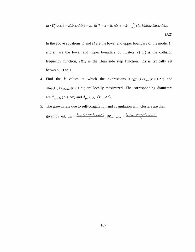
167
∆𝜏 ∙ ∫ 𝑐(𝑥, 𝑘 − 𝑥)��(𝑥, 𝜏)��(𝑘 − 𝑥, 𝜏)𝐻(𝑘 − 𝑥 − 𝐻𝑐)𝑑𝑥𝐻𝑐
𝐿𝑐+ −∆𝜏 ∙ ∫ 𝑐(𝑥, 𝑘)��(𝑥, 𝜏)��(𝑘, 𝜏)𝑑𝑥
𝐻𝑐
𝐿𝑐.
(A2)
In the above equations, L and H are the lower and upper boundary of the mode, 𝐿𝑐
and 𝐻𝑐 are the lower and upper boundary of clusters, 𝑐(𝑖, 𝑗) is the collision
frequency function, H(x) is the Heaviside step function. ∆𝜏 is typically set
between 0.1 to 1.
4. Find the k values at which the expressions 3 log(10) 𝑘��𝑠𝑒𝑙𝑓(𝑘, 𝜏 + ∆𝜏) and
3 log(10) 𝑘��𝑐𝑙𝑢𝑠𝑡𝑒𝑟(𝑘, 𝜏 + ∆𝜏) are locally maximized. The corresponding diameters
are ��𝑝,𝑠𝑒𝑙𝑓(𝜏 + ∆𝜏) and ��𝑝,𝑐𝑙𝑢𝑠𝑡𝑒𝑟(𝜏 + ∆𝜏).
5. The growth rate due to self-coagulation and coagulation with clusters are then
given by 𝐺𝑅𝑚,𝑠𝑒𝑙𝑓 =��𝑝,𝑠𝑒𝑙𝑓(𝜏+∆𝜏)−��𝑝,𝑚𝑜𝑑𝑒(𝜏)
∆𝜏; 𝐺𝑅𝑚,𝑐𝑙𝑢𝑠𝑡𝑒𝑟 =
��𝑝,𝑐𝑙𝑢𝑠𝑡𝑒𝑟(𝜏+∆𝜏)−��𝑝,𝑚𝑜𝑑𝑒(𝜏)
∆𝜏 .
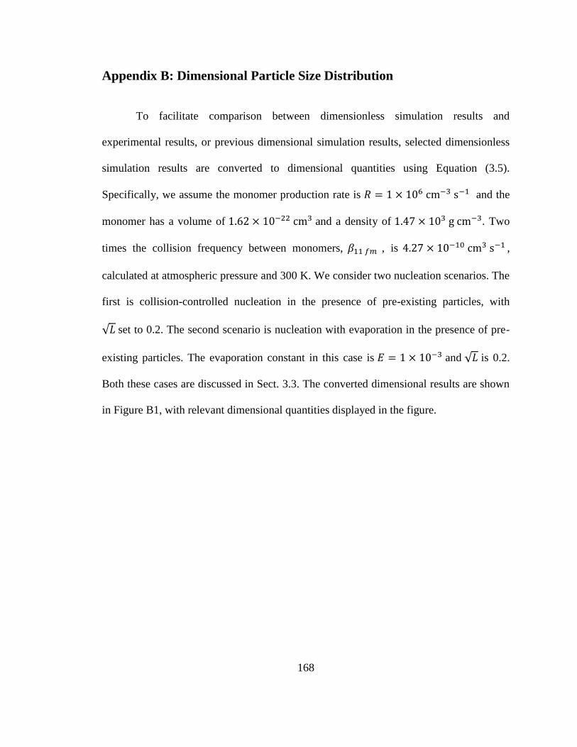
168
Appendix B: Dimensional Particle Size Distribution
To facilitate comparison between dimensionless simulation results and
experimental results, or previous dimensional simulation results, selected dimensionless
simulation results are converted to dimensional quantities using Equation (3.5).
Specifically, we assume the monomer production rate is 𝑅 = 1 × 106 cm−3 s−1 and the
monomer has a volume of 1.62 × 10⁻²² cm3 and a density of 1.47 × 10³ g cm−3. Two
times the collision frequency between monomers, 𝛽11 𝑓𝑚 , is 4.27 × 10⁻¹⁰ cm3 s−1 ,
calculated at atmospheric pressure and 300 K. We consider two nucleation scenarios. The
first is collision-controlled nucleation in the presence of pre-existing particles, with
√𝐿 set to 0.2. The second scenario is nucleation with evaporation in the presence of pre-
existing particles. The evaporation constant in this case is 𝐸 = 1 × 10⁻³ and √𝐿 is 0.2.
Both these cases are discussed in Sect. 3.3. The converted dimensional results are shown
in Figure B1, with relevant dimensional quantities displayed in the figure.
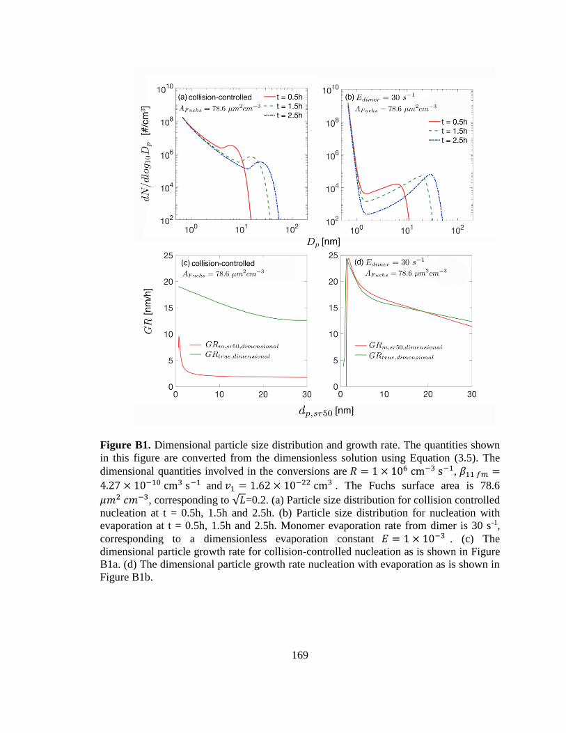
169
Figure B1. Dimensional particle size distribution and growth rate. The quantities shown
in this figure are converted from the dimensionless solution using Equation (3.5). The
dimensional quantities involved in the conversions are 𝑅 = 1 × 106 cm−3 s−1, 𝛽11 𝑓𝑚 =
4.27 × 10⁻¹⁰ cm3 s−1 and 𝑣1 = 1.62 × 10⁻²² cm3 . The Fuchs surface area is 78.6
𝜇𝑚2 𝑐𝑚−3, corresponding to √𝐿=0.2. (a) Particle size distribution for collision controlled
nucleation at t = 0.5h, 1.5h and 2.5h. (b) Particle size distribution for nucleation with
evaporation at t = 0.5h, 1.5h and 2.5h. Monomer evaporation rate from dimer is 30 s-1,
corresponding to a dimensionless evaporation constant 𝐸 = 1 × 10⁻³ . (c) The
dimensional particle growth rate for collision-controlled nucleation as is shown in Figure
B1a. (d) The dimensional particle growth rate nucleation with evaporation as is shown in
Figure B1b.

170
Appendix C: Additional Langmuir Model Fitting Results and Mass-
mobility Spectra
Figure C1. Langmuir model fitting for (a) (NaCl)xNa+ (x=1, 13) and (b) (NaCl)xCl-
(x=1,4,9,13).

171
Figure C2. Contour plot for positively charged sodium chloride cluster ions at Pc = 48Pa
(Pc is the vapor pressure of chlorobutane in the DMA). Compared with Figure 4.1 of the
main text, more noise (signal not attributed to cluster ions) is detected and signal line
segments are elongated, indicating degraded system resolution (often the result of
transient binding of impurities).

172
Appendix D: Calculation of Zg
The mobility of a cluster ion with g number of vapor molecules bound, used in
Langmuir model fitting, was calculated as follows. First, an effective diameter of the dry
cluster, d0, was inferred from the dry mobility using the following equation from Larriba
& Hogan (2013):
𝑍0 =3𝑧𝑒
𝜋𝜉𝜌𝑔𝑎𝑠𝑐𝑔𝑎𝑠(𝑑0+𝑑𝑔𝑎𝑠)2𝐿(𝜓𝑝𝑜𝑙,0)
(D1a)
𝜓𝑝𝑜𝑙,0 =2𝛼𝑝𝑜𝑙𝑧
2𝑒2
𝜋𝜀𝑜𝑘𝐵𝑇(𝑑0+𝑑𝑔𝑎𝑠)4 (D1b)
𝐿(𝜓𝑝𝑜𝑙,𝑘) = 1 + 𝜓𝑝𝑜𝑙,𝑘 (1
3.1+
1
𝜉(
1
16+
4
33𝜓𝑝𝑜𝑙,𝑘)) if 𝜓𝑝𝑜𝑙,𝑘 ≤ 1 (D1c)
𝐿(𝜓𝑝𝑜𝑙,𝑘) = 1 + 𝜓𝑝𝑜𝑙,𝑘 (1
4−
2.3
1000𝜓𝑝𝑜𝑙,𝑘 +
1
𝜉(
9
56−
6.8
1000𝜓𝑝𝑜𝑙,𝑘)) if 𝜓𝑝𝑜𝑙,𝑘 > 1
(D1d)
where Z0 is the mobility measured under dry conditions, z is the charge state, e is the unit
electron charge, 𝜉 is the momentum scattering factor (1.36), 𝜌𝑔𝑎𝑠 is the gas mass density,
𝑐𝑔𝑎𝑠 is the mean thermal speed of the gas molecule-cluster reduced mass, 𝐿(𝜓𝑝𝑜𝑙,0) is the
polarization correction factor, 𝜓𝑝𝑜𝑙,0 is the polarization energy at collision, 𝛼𝑝𝑜𝑙 is the gas
molecule polarizability (1.7 x 10⁻³⁰ m3), kB is Boltzmann’s constant, T is the gas
temperature, and dgas is the gas molecule diameter (0.3 nm). Subsequently, dg, the
effective diameter of a cluster with g vapor molecules bound was estimated using the
equation:
𝑑𝑔 = (𝑑03 +
6
𝜋𝑔𝑣)
1/3
(D2)
173
where v is the effective molecular volume of the condensed vapor (estimated from bulk
properties). With dg, Zg is then calculated applying Equations (D1a-d) but substituting dg
for d0.
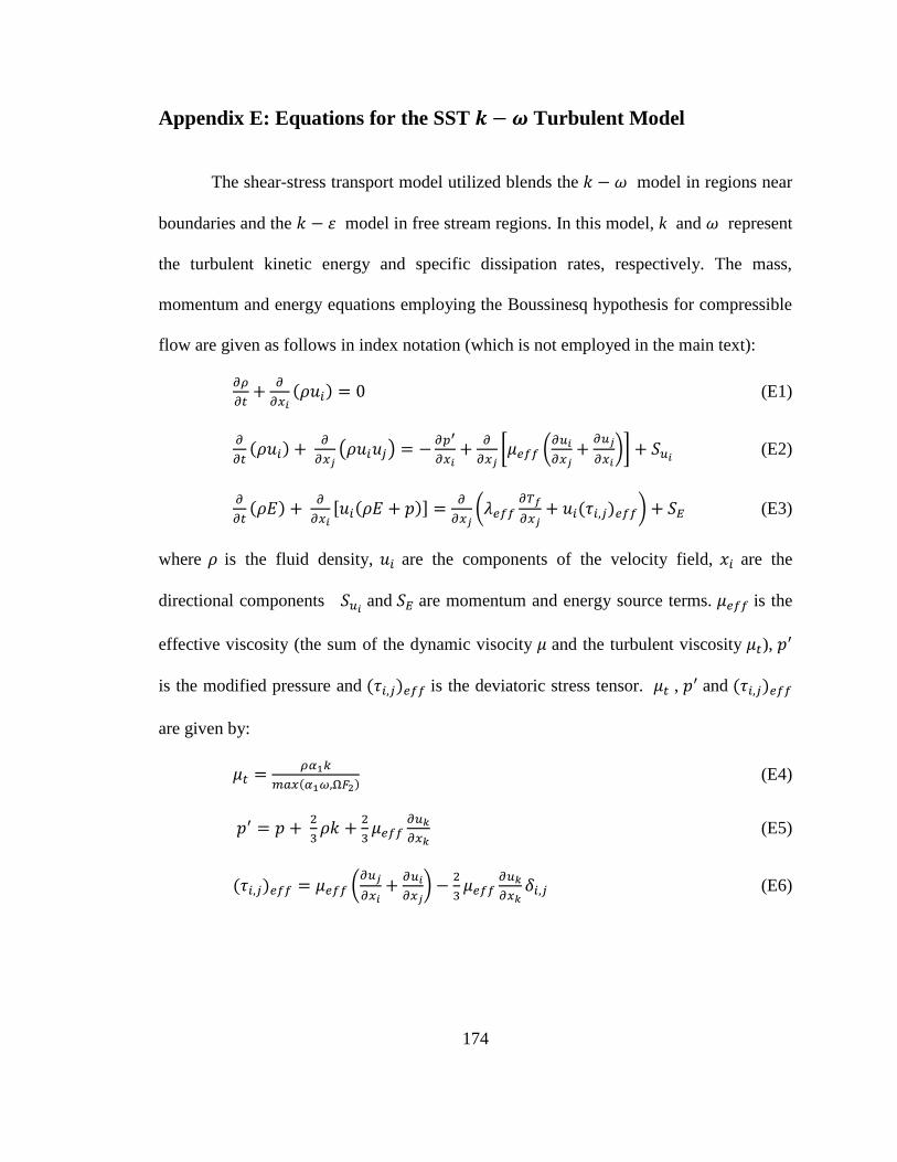
174
Appendix E: Equations for the SST 𝒌 − 𝝎 Turbulent Model
The shear-stress transport model utilized blends the 𝑘 − 𝜔 model in regions near
boundaries and the 𝑘 − 휀 model in free stream regions. In this model, k and 𝜔 represent
the turbulent kinetic energy and specific dissipation rates, respectively. The mass,
momentum and energy equations employing the Boussinesq hypothesis for compressible
flow are given as follows in index notation (which is not employed in the main text):
𝜕𝜌
𝜕𝑡+
𝜕
𝜕𝑥𝑖(𝜌𝑢𝑖) = 0 (E1)
𝜕
𝜕𝑡(𝜌𝑢𝑖) +
𝜕
𝜕𝑥𝑗(𝜌𝑢𝑖𝑢𝑗) = −
𝜕𝑝′
𝜕𝑥𝑖+
𝜕
𝜕𝑥𝑗[𝜇𝑒𝑓𝑓 (
𝜕𝑢𝑖
𝜕𝑥𝑗+
𝜕𝑢𝑗
𝜕𝑥𝑖)] + 𝑆𝑢𝑖
(E2)
𝜕
𝜕𝑡(𝜌𝐸) +
𝜕
𝜕𝑥𝑖[𝑢𝑖(𝜌𝐸 + 𝑝)] =
𝜕
𝜕𝑥𝑗(𝜆𝑒𝑓𝑓
𝜕𝑇𝑓
𝜕𝑥𝑗+ 𝑢𝑖(𝜏𝑖,𝑗)𝑒𝑓𝑓) + 𝑆𝐸 (E3)
where 𝜌 is the fluid density, 𝑢𝑖 are the components of the velocity field, 𝑥𝑖 are the
directional components 𝑆𝑢𝑖 and 𝑆𝐸 are momentum and energy source terms. 𝜇𝑒𝑓𝑓 is the
effective viscosity (the sum of the dynamic visocity 𝜇 and the turbulent viscosity 𝜇𝑡), 𝑝′
is the modified pressure and (𝜏𝑖,𝑗)𝑒𝑓𝑓 is the deviatoric stress tensor. 𝜇𝑡 , 𝑝′ and (𝜏𝑖,𝑗)𝑒𝑓𝑓
are given by:
𝜇𝑡 =𝜌𝛼1𝑘
𝑚𝑎𝑥(𝛼1𝜔,Ω𝐹2) (E4)
𝑝′ = 𝑝 + 2
3𝜌𝑘 +
2
3𝜇𝑒𝑓𝑓
𝜕𝑢𝑘
𝜕𝑥𝑘 (E5)
(𝜏𝑖,𝑗)𝑒𝑓𝑓 = 𝜇𝑒𝑓𝑓 (𝜕𝑢𝑗
𝜕𝑥𝑖+
𝜕𝑢𝑖
𝜕𝑥𝑗) −
2
3𝜇𝑒𝑓𝑓
𝜕𝑢𝑘
𝜕𝑥𝑘𝛿𝑖,𝑗 (E6)

175
where Ω is the strain rate constant, 𝛼1 is an input model constant, 𝐹2 is a blending
function, and 𝛿𝑖,𝑗 is the Kronecker delta function. The transport equation of turbulent
kinetic energy (k) and specific dissipation rate (𝜔) are given by:
𝜕
𝜕𝑡(𝜌𝑘) +
𝜕
𝜕𝑥𝑖(𝜌𝑘𝑢𝑖) =
𝜕
𝜕𝑥𝑗((𝜇 +
𝜇𝑡
𝜎𝑘)
𝜕𝑘
𝜕𝑥𝑗) + 𝐺𝑘 − 𝑌𝑘 (E7)
𝜕
𝜕𝑡(𝜌𝜔) +
𝜕
𝜕𝑥𝑗(𝜌𝜔𝑢𝑗) =
𝜕
𝜕𝑥𝑗((𝜇 +
𝜇𝑡
𝜎𝑤)
𝜕𝜔
𝜕𝑥𝑗) + 𝐺𝜔 − 𝑌𝜔 + 𝐷𝜔 (E8)
where σ𝑘 and σ𝜔 are the turbulent Prantl numbers of k and 𝜔, respectively, 𝐺𝑘 and 𝐺𝜔
are the production terms of k and 𝜔, 𝑌𝑘 and 𝑌𝜔 are the dissipation terms of k and 𝜔 due to
turbulence, 𝐷𝜔 is the cross diffusion term (𝐷𝑤+ represents the positive portion of the cross
diffusion term). σ𝑘, σ𝜔, 𝐷𝜔, 𝐷𝜔+ together with the blending functions 𝐹1 and 𝐹2 are given
by :
σ𝑘 =1
𝐹1𝜎𝑘,1
+(1−𝐹1)
𝜎𝑘,2
(E9)
σ𝜔 =1
𝐹1𝜎𝜔,1
+(1−𝐹1)
𝜎𝜔,2
(E10)
𝐷𝜔 =2𝜌
𝜎𝑤,2𝜔
𝜕𝑘
𝜕𝑥𝑗
𝜕𝜔
𝜕𝑥𝑗 (E11)
𝐷𝑤+ = 𝑚𝑎𝑥 [
2𝜌
𝜎𝑤,2𝜔
𝜕𝑘
𝜕𝑥𝑗
𝜕𝜔
𝜕𝑥𝑗, 10−10] (E12)
𝐹1 = tanh(Φ14) , Φ1 = min [𝑚𝑎𝑥 (
√𝑘
0.09𝜔𝑦,500𝜇
𝜌𝑦2𝜔) ,
4𝜌𝑘
𝜎𝑤,2𝐷𝑤+𝑦2] (E13)
𝐹2 = tanh(Φ12)Φ2 = max (
√𝑘
0.09𝜔𝑦,500𝜇
𝜌𝑦2𝜔) (E14)
where 𝜎𝑘,1, 𝜎𝑘,2, 𝜎𝜔,1 and 𝜎𝜔,2 are model constants. The production and dissipation term
of k and 𝜔 are given by
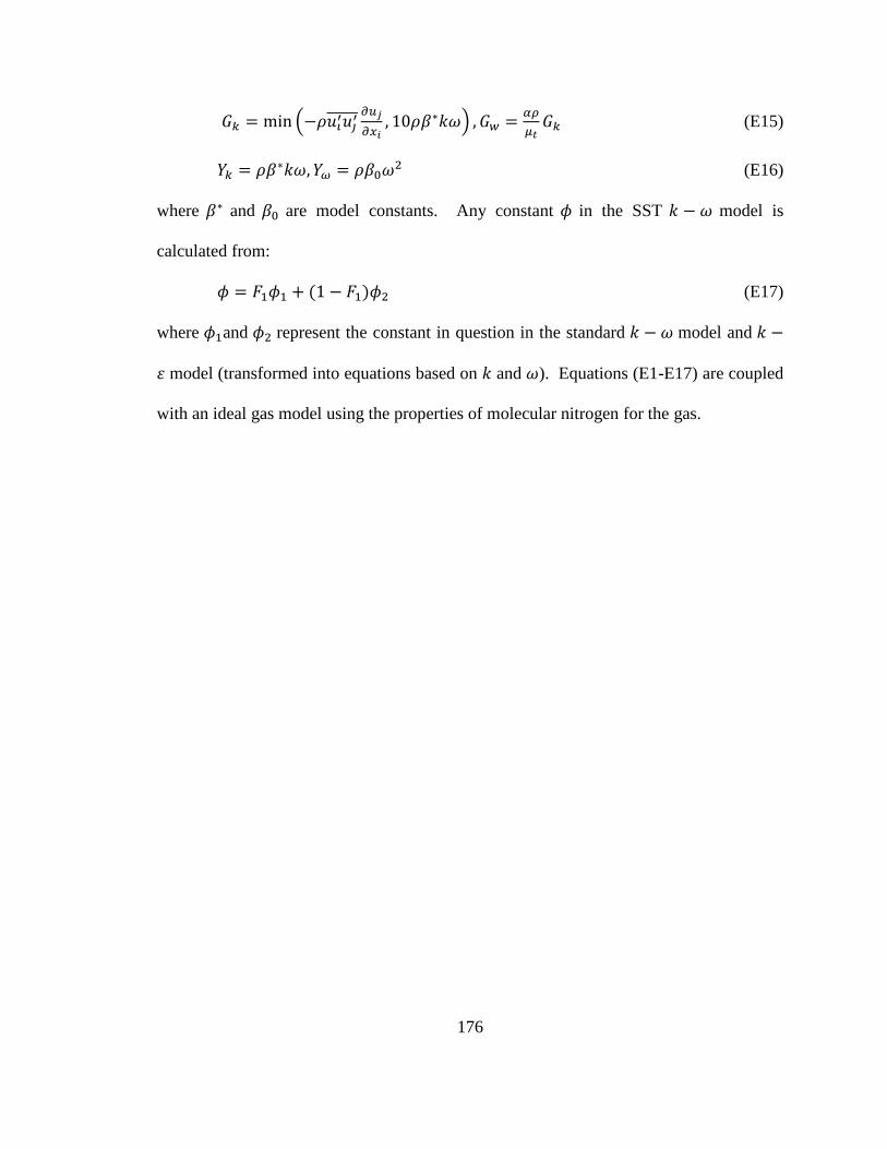
176
𝐺𝑘 = min (−𝜌𝑢𝑖′𝑢𝑗
′ 𝜕𝑢𝑗
𝜕𝑥𝑖, 10𝜌𝛽∗𝑘𝜔) , 𝐺𝑤 =
𝛼𝜌
𝜇𝑡𝐺𝑘 (E15)
𝑌𝑘 = 𝜌𝛽∗𝑘𝜔, 𝑌𝜔 = 𝜌𝛽0𝜔2 (E16)
where 𝛽∗ and 𝛽0 are model constants. Any constant 𝜙 in the SST 𝑘 − 𝜔 model is
calculated from:
𝜙 = 𝐹1𝜙1 + (1 − 𝐹1)𝜙2 (E17)
where 𝜙1and 𝜙2 represent the constant in question in the standard 𝑘 − 𝜔 model and 𝑘 −
휀 model (transformed into equations based on 𝑘 and 𝜔). Equations (E1-E17) are coupled
with an ideal gas model using the properties of molecular nitrogen for the gas.
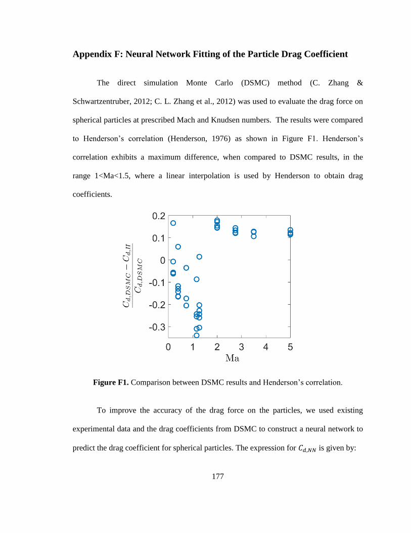
177
Appendix F: Neural Network Fitting of the Particle Drag Coefficient
The direct simulation Monte Carlo (DSMC) method (C. Zhang &
Schwartzentruber, 2012; C. L. Zhang et al., 2012) was used to evaluate the drag force on
spherical particles at prescribed Mach and Knudsen numbers. The results were compared
to Henderson’s correlation (Henderson, 1976) as shown in Figure F1. Henderson’s
correlation exhibits a maximum difference, when compared to DSMC results, in the
range 1<Ma<1.5, where a linear interpolation is used by Henderson to obtain drag
coefficients.
Figure F1. Comparison between DSMC results and Henderson’s correlation.
To improve the accuracy of the drag force on the particles, we used existing
experimental data and the drag coefficients from DSMC to construct a neural network to
predict the drag coefficient for spherical particles. The expression for 𝐶𝑑,𝑁𝑁 is given by:
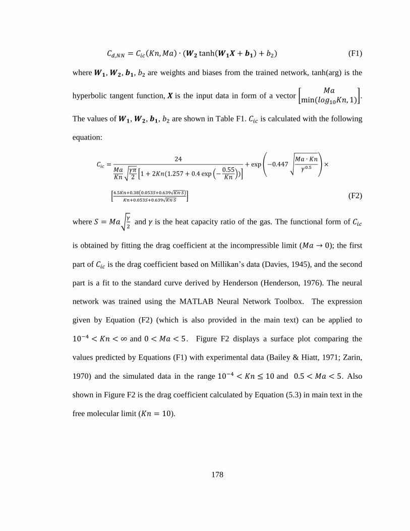
178
𝐶𝑑,𝑁𝑁 = 𝐶𝑖𝑐(𝐾𝑛,𝑀𝑎) ∙ (𝑾𝟐 tanh(𝑾𝟏𝑿 + 𝒃𝟏) + 𝑏2) (F1)
where 𝑾𝟏, 𝑾𝟐, 𝒃𝟏, 𝑏2 are weights and biases from the trained network, tanh(arg) is the
hyperbolic tangent function, 𝑿 is the input data in form of a vector [𝑀𝑎
min (𝑙𝑜𝑔10𝐾𝑛, 1)].
The values of 𝑾𝟏, 𝑾𝟐, 𝒃𝟏, 𝑏2 are shown in Table F1. 𝐶𝑖𝑐 is calculated with the following
equation:
𝐶𝑖𝑐 =24
𝑀𝑎𝐾𝑛
√𝛾𝜋2
[1 + 2𝐾𝑛(1.257 + 0.4 exp (−0.55𝐾𝑛
))]
+ exp (−0.447 √𝑀𝑎 ∙ 𝐾𝑛
𝛾0.5) ×
[4.5𝐾𝑛+0.38(0.053𝑆+0.639√𝐾𝑛∙𝑆)
𝐾𝑛+0.053𝑆+0.639√𝐾𝑛∙𝑆] (F2)
where 𝑆 = 𝑀𝑎√𝛾
2 and 𝛾 is the heat capacity ratio of the gas. The functional form of 𝐶𝑖𝑐
is obtained by fitting the drag coefficient at the incompressible limit (𝑀𝑎 → 0); the first
part of 𝐶𝑖𝑐 is the drag coefficient based on Millikan’s data (Davies, 1945), and the second
part is a fit to the standard curve derived by Henderson (Henderson, 1976). The neural
network was trained using the MATLAB Neural Network Toolbox. The expression
given by Equation (F2) (which is also provided in the main text) can be applied to
10−4 < 𝐾𝑛 < ∞ and 0 < 𝑀𝑎 < 5 . Figure F2 displays a surface plot comparing the
values predicted by Equations (F1) with experimental data (Bailey & Hiatt, 1971; Zarin,
1970) and the simulated data in the range 10−4 < 𝐾𝑛 ≤ 10 and 0.5 < 𝑀𝑎 < 5. Also
shown in Figure F2 is the drag coefficient calculated by Equation (5.3) in main text in the
free molecular limit (𝐾𝑛 = 10).

179
Figure F2. (a) Comparison of the drag coefficient given by equation (F1) with
experimental data, simulated results (obtained by DSMC) and theoretical values in the
free molecular limit. (b), (c), (d) and (e) are comparisons between neural net predictions
and experimental data as well as DSMC results at Mach number 0.4, 1.16, 3.0 and 5.0,
respectively.
Table F1. Values of weights and biases in Equation (F18). 𝑾𝟏 is a 𝟐𝟎 × 𝟐 matrix, 𝒃𝟏 is
a 𝟐𝟎 × 𝟏 matrix and 𝑾𝟐 is a 𝟏 × 𝟐𝟎 matrix. Note it is the transpose of 𝑾𝟐, 𝑾𝟐𝑻 that is
listed in this table. 𝒃𝟐 is a scalar with a value of 2.9633 and is not shown in the table.
𝑾𝟏 𝒃𝟏 𝑾𝟐𝑻
-2.4007 1.746 13.9004 -1.1289
-0.6223 2.1452 11.4413 -0.0787
-2.106 1.483 12.0261 1.3958
1.0772 -2.211 -11.1729 0.1424
-0.0941 -0.2127 1.1092 -5.3498
-1.7974 -0.4568 6.2976 0.1227
-1.5316 1.125 7.2065 0.345
0.918 -1.0428 -5.3537 0.6979
-2.6393 0.2688 5.4774 -0.8946
0.1141 1.0503 0.7186 -0.6304
-0.0921 2.2469 4.152 -0.2392
-1.8866 0.3119 3.9608 2.5038
-0.8746 1.5139 4.6805 -0.3205
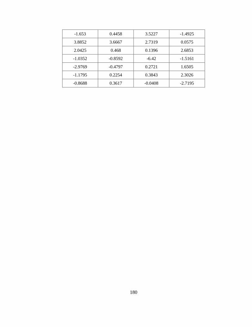
180
-1.653 0.4458 3.5227 -1.4925
3.8852 3.6667 2.7319 0.0575
2.0425 0.468 0.1396 2.6853
-1.0352 -0.8592 -6.42 -1.5161
-2.9769 -0.4797 0.2721 1.6505
-1.1795 0.2254 0.3843 2.3026
-0.8688 0.3617 -0.0408 -2.7195
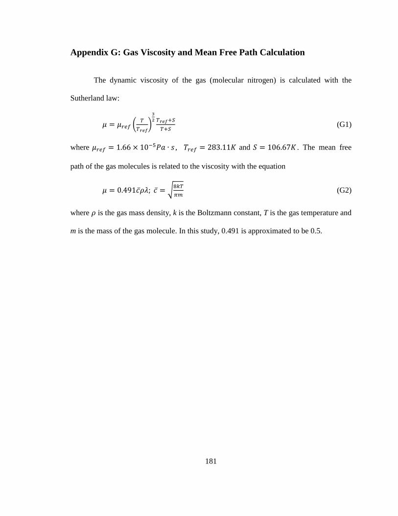
181
Appendix G: Gas Viscosity and Mean Free Path Calculation
The dynamic viscosity of the gas (molecular nitrogen) is calculated with the
Sutherland law:
𝜇 = 𝜇𝑟𝑒𝑓 (𝑇
𝑇𝑟𝑒𝑓)
3
2 𝑇𝑟𝑒𝑓+𝑆
𝑇+𝑆 (G1)
where 𝜇𝑟𝑒𝑓 = 1.66 × 10⁻⁵𝑃𝑎 ∙ 𝑠 , 𝑇𝑟𝑒𝑓 = 283.11𝐾 and 𝑆 = 106.67𝐾 . The mean free
path of the gas molecules is related to the viscosity with the equation
𝜇 = 0.491𝑐𝜌𝜆; 𝑐 = √8𝑘𝑇
𝜋𝑚 (G2)
where 𝜌 is the gas mass density, k is the Boltzmann constant, T is the gas temperature and
m is the mass of the gas molecule. In this study, 0.491 is approximated to be 0.5.
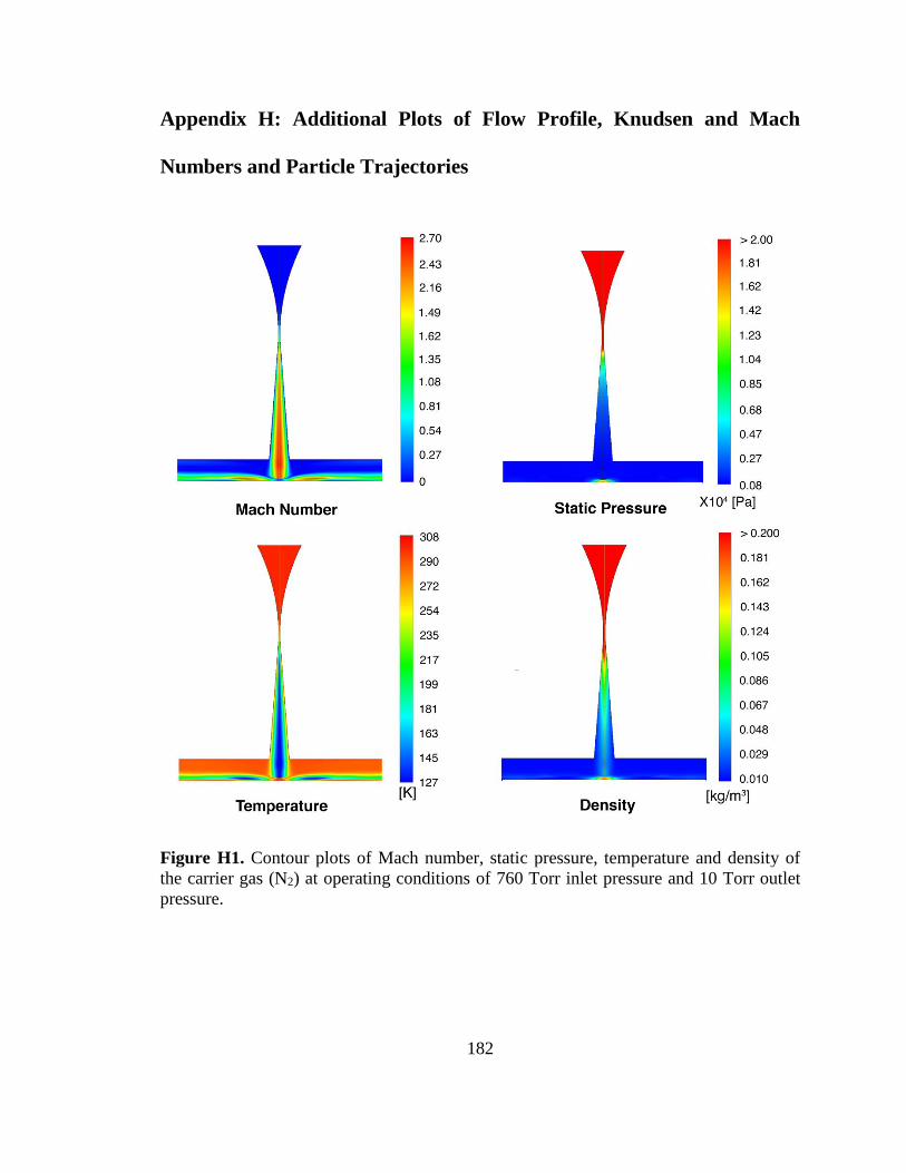
182
Appendix H: Additional Plots of Flow Profile, Knudsen and Mach
Numbers and Particle Trajectories
Figure H1. Contour plots of Mach number, static pressure, temperature and density of
the carrier gas (N2) at operating conditions of 760 Torr inlet pressure and 10 Torr outlet
pressure.
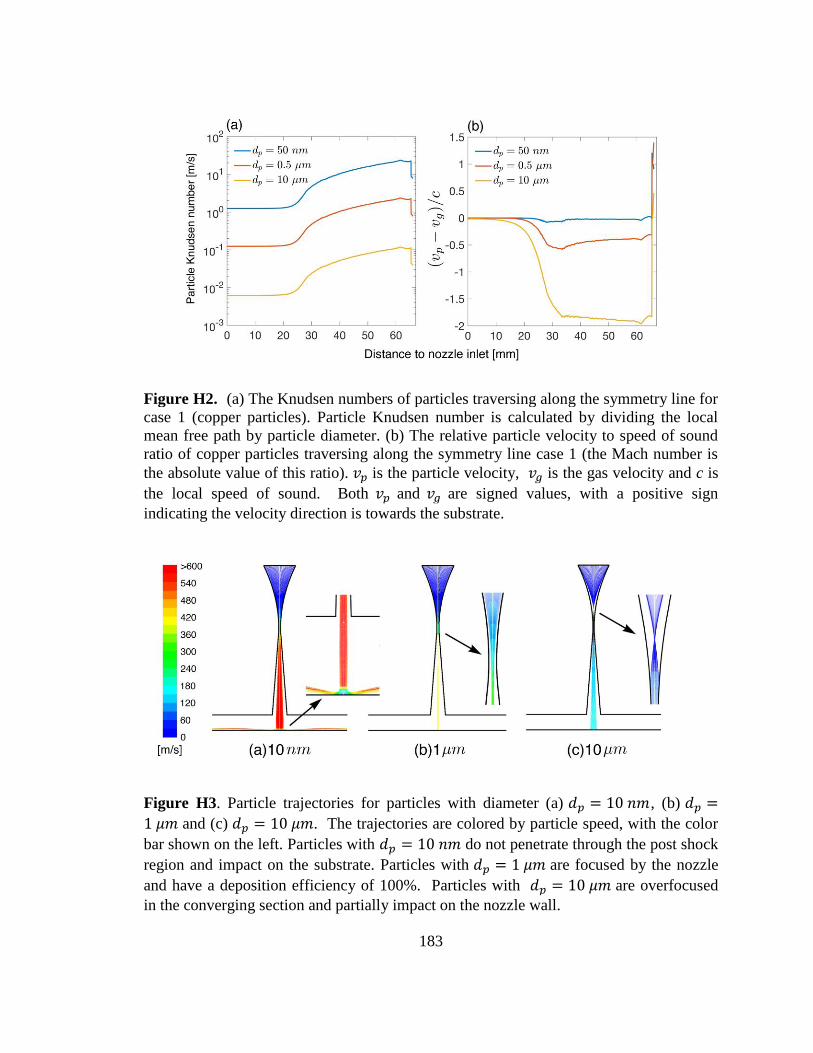
183
Figure H2. (a) The Knudsen numbers of particles traversing along the symmetry line for
case 1 (copper particles). Particle Knudsen number is calculated by dividing the local
mean free path by particle diameter. (b) The relative particle velocity to speed of sound
ratio of copper particles traversing along the symmetry line case 1 (the Mach number is
the absolute value of this ratio). 𝑣𝑝 is the particle velocity, 𝑣𝑔 is the gas velocity and c is
the local speed of sound. Both 𝑣𝑝 and 𝑣𝑔 are signed values, with a positive sign
indicating the velocity direction is towards the substrate.
Figure H3. Particle trajectories for particles with diameter (a) 𝑑𝑝 = 10 𝑛𝑚, (b) 𝑑𝑝 =
1 𝜇𝑚 and (c) 𝑑𝑝 = 10 𝜇𝑚. The trajectories are colored by particle speed, with the color
bar shown on the left. Particles with 𝑑𝑝 = 10 𝑛𝑚 do not penetrate through the post shock
region and impact on the substrate. Particles with 𝑑𝑝 = 1 𝜇𝑚 are focused by the nozzle
and have a deposition efficiency of 100%. Particles with 𝑑𝑝 = 10 𝜇𝑚 are overfocused
in the converging section and partially impact on the nozzle wall.
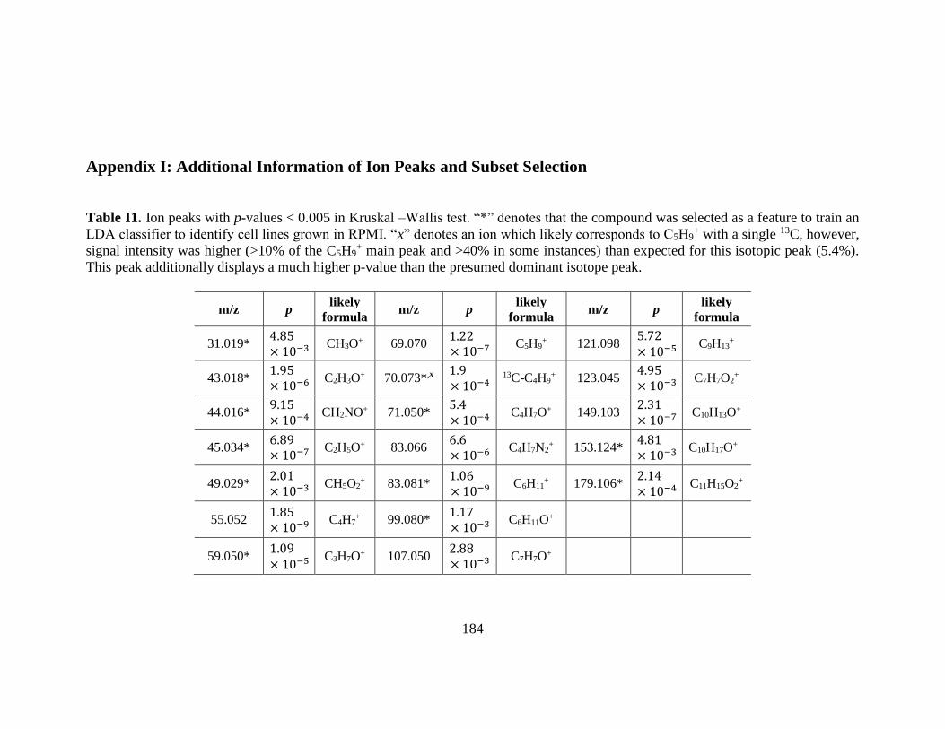
184
Appendix I: Additional Information of Ion Peaks and Subset Selection
Table I1. Ion peaks with p-values < 0.005 in Kruskal –Wallis test. “*” denotes that the compound was selected as a feature to train an
LDA classifier to identify cell lines grown in RPMI. “x” denotes an ion which likely corresponds to C5H9+ with a single 13C, however,
signal intensity was higher (>10% of the C5H9+ main peak and >40% in some instances) than expected for this isotopic peak (5.4%).
This peak additionally displays a much higher p-value than the presumed dominant isotope peak.
m/z p likely
formula m/z p
likely
formula m/z p
likely
formula
31.019* 4.85× 10−3
CH3O+ 69.070 1.22× 10⁻⁷
C5H9+ 121.098
5.72× 10⁻⁵
C9H13+
43.018* 1.95× 10−6
C2H3O+ 70.073*,x 1.9× 10⁻⁴
13C-C4H9+ 123.045
4.95× 10⁻³
C7H7O2+
44.016* 9.15× 10−4
CH2NO+ 71.050* 5.4× 10−4
C4H7O+ 149.103 2.31× 10⁻⁷
C10H13O+
45.034* 6.89× 10−7
C2H5O+ 83.066 6.6× 10⁻⁶
C4H7N2+ 153.124*
4.81× 10−3
C10H17O+
49.029* 2.01× 10−3
CH5O2+ 83.081*
1.06× 10−9
C6H11+ 179.106*
2.14× 10−4
C11H15O2+
55.052 1.85× 10⁻⁹
C4H7+ 99.080*
1.17× 10−3
C6H11O+
59.050* 1.09× 10−5
C3H7O+ 107.050 2.88× 10⁻³
C7H7O+
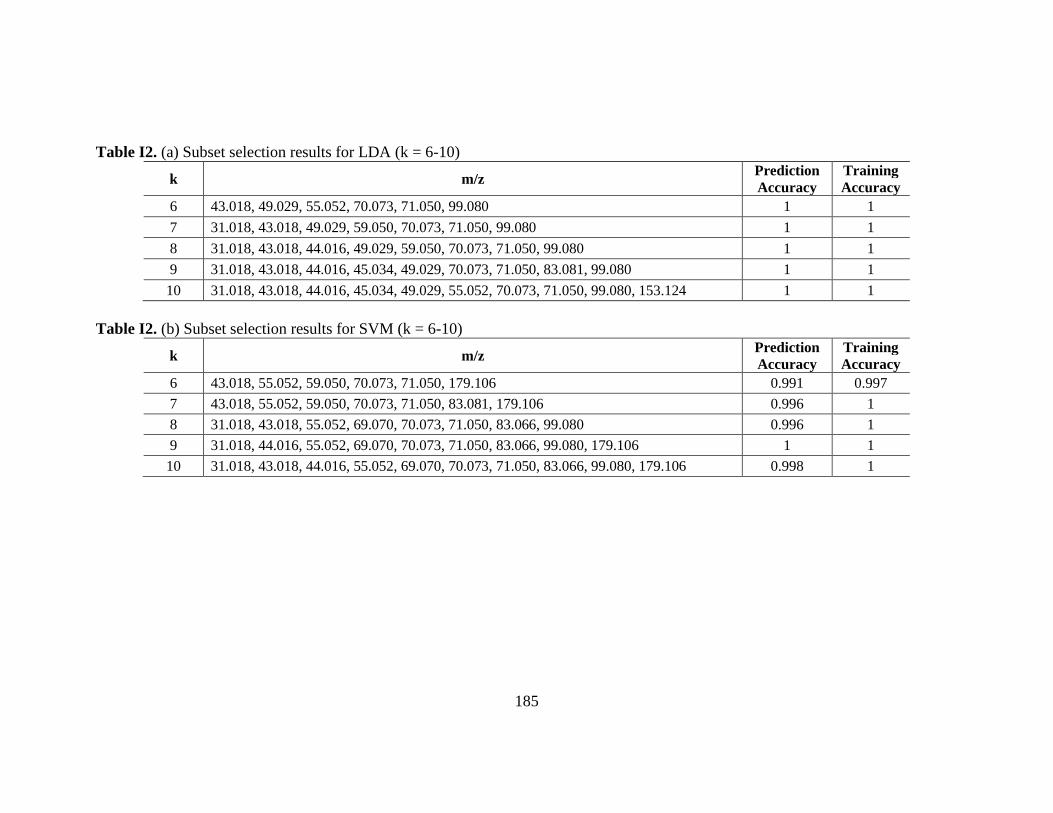
185
Table I2. (a) Subset selection results for LDA (k = 6-10)
k m/z Prediction
Accuracy
Training
Accuracy
6 43.018, 49.029, 55.052, 70.073, 71.050, 99.080 1 1
7 31.018, 43.018, 49.029, 59.050, 70.073, 71.050, 99.080 1 1
8 31.018, 43.018, 44.016, 49.029, 59.050, 70.073, 71.050, 99.080 1 1
9 31.018, 43.018, 44.016, 45.034, 49.029, 70.073, 71.050, 83.081, 99.080 1 1
10 31.018, 43.018, 44.016, 45.034, 49.029, 55.052, 70.073, 71.050, 99.080, 153.124 1 1
Table I2. (b) Subset selection results for SVM (k = 6-10)
k m/z Prediction
Accuracy
Training
Accuracy
6 43.018, 55.052, 59.050, 70.073, 71.050, 179.106 0.991 0.997
7 43.018, 55.052, 59.050, 70.073, 71.050, 83.081, 179.106 0.996 1
8 31.018, 43.018, 55.052, 69.070, 70.073, 71.050, 83.066, 99.080 0.996 1
9 31.018, 44.016, 55.052, 69.070, 70.073, 71.050, 83.066, 99.080, 179.106 1 1
10 31.018, 43.018, 44.016, 55.052, 69.070, 70.073, 71.050, 83.066, 99.080, 179.106 0.998 1