Particle Filtering and Moving Horizon Estimation

A

mTmfi©

K

1

fikmttcomttrOotvtatbt

0d

Computers and Chemical Engineering 30 (2006) 1529–1541

Particle filtering and moving horizon estimation

James B. Rawlings a,∗, Bhavik R. Bakshi b

a Department of Chemical and Biological Engineering, University of Wisconsin, Madison, United Statesb Department of Chemical and Biomolecular Engineering, Ohio State University, United States

Received 6 March 2006; received in revised form 18 May 2006; accepted 22 May 2006Available online 21 July 2006

bstract

This paper provides an overview of currently available methods for state estimation of linear, constrained and nonlinear systems. The followingethods are discussed: Kalman filtering, extended Kalman filtering, unscented Kalman filtering, particle filtering, and moving horizon estimation.
he current research literature on particle filtering and moving horizon estimation is reviewed, and the advantages and disadvantages of theseethods are presented. Topics for new research are suggested that address combining the best features of moving horizon estimation and particlelters.2006 Elsevier Ltd. All rights reserved.
c

x

y

i

•

•

•

•

•

eywords: State estimation; Particle filtering; Moving horizon estimation

. Introduction

The fundamental question of state estimation arises in manyelds of science and engineering. How does one best combinenowledge from two sources – an a priori model and onlineeasurements – from a dynamic system in real time to estimate

he state of the dynamic system. Because of its wide applica-ion, many different scientific and engineering disciplines haveontributed to our understanding of state estimation. The fieldsf systems theory, statistics and applied probability, as well asany different applications areas have contributed underlying

heory, methods, and computational algorithms for state estima-ion. The purpose of this review is to assess some of the moreecent and more active areas of this diverse research literature.ur goal is to summarize the state of the art and point out somef the current research directions that show promise for applica-ion in the area of process systems and control. Because of theery wide scope of the state estimation problem, we are forcedo limit the review to only those parts of the field with which theuthors have some direct knowledge or experience. Even with
his restricted scope, we found it necessary to provide only arief overview of the many different methods, and focus atten-ion mainly on recent developments.
∗ Corresponding author.E-mail address: [email protected] (J.B. Rawlings).

••

tn.

098-1354/$ – see front matter © 2006 Elsevier Ltd. All rights reserved.oi:10.1016/j.compchemeng.2006.05.031

For the purposes of this paper we consider the following dis-rete time dynamic system

(k + 1) = F (x(k), u(k)) + G(x(k), u(k))w(k) (1a)

(k) = h(x(k)) + v(k) (1b)

n which

x(k) is the state of the system at time t(k). The initial value,x(0), is a random variable with a given density;u(k) is the system input at time t(k) (assumes a zero-order holdover the time interval [t(k),t(k + 1)];w(k) and v(k) are sequences of independent random vari-ables, called process and measurement noises, respectively,with time-invariant densities;F(x(k), u(k)) is a (possibly) nonlinear system model. F may bethe solution to a first principles, differential equation model;G(x(k), u(k)) is a full column rank matrix (this conditionis required for uniqueness of the conditional density to bedefined later;y(k) is the system measurement or observation at time t(k);h is a (possibly) nonlinear function of x(k).

The state estimation problem is to determine an estimate ofhe state x(T) given the chosen model structure and a sequence ofoisy observations (measurements) of the system, Y(T) := {y(0),. ., y(T)}. As might be expected from such a fundamental

mailto:[email protected]

dx.doi.org/10.1016/j.compchemeng.2006.05.031

1 d Chemical Engineering 30 (2006) 1529–1541

ptsmtstflcpnoosesrioe((

usnsfifDmwaaaiBpcetwotdttac

apmiew

Fa

oisi((Sod1ttCGmpan(ogamv

n(ob

530 J.B. Rawlings, B.R. Bakshi / Computers an

roblem statement, state estimation has found diverse applica-ion in science and engineering over many years. In the stochasticetting chosen here, the conditional density of the state given theeasurements, px|Y(x(T)|Y(T)) is the natural statistical distribu-

ion of interest, and the state estimation problem is essentiallyolved if we can find this distribution. The complete condi-ional density is difficult to calculate exactly, however, exceptor well-known simple systems, such as when F and G areinear, and w and v are normally distributed. In this case theonditional density is also Gaussian with mean and covariancerovided by the well-known Kalman filter. When F and G areonlinear, however, the conditional density is not Gaussian, andbtaining a complete solution is generally impractical. More-ver, when state estimation is used as part of a feedback controlystem, the state estimator must meet other requirements. Thestimate must be found during the available sample time of theystem as each measurement becomes available. The on-lineequirements provide further limitations on what is achievablen state estimation. In this review, we consider many of the meth-ds for solving this problem including Kalman filtering (KF),xtended Kalman filtering (EKF), unscented Kalman filteringUKF), particle filtering (PF), and moving horizon estimationMHE).

Although the Kalman filter is the optimal state estimator fornconstrained, linear systems subject to normally distributedtate and measurement noise, many physical systems, exhibitonlinear dynamics and have states subject to hard constraints,uch as nonnegative concentrations or pressures. Hence Kalmanltering is no longer directly applicable. As a result, many dif-erent types of nonlinear state estimators have been proposed;aum (2005) provides a highly readable and tutorial summary ofany of these methods, and Soroush (1998) provides a reviewith a focus on applications in process control. We focus our

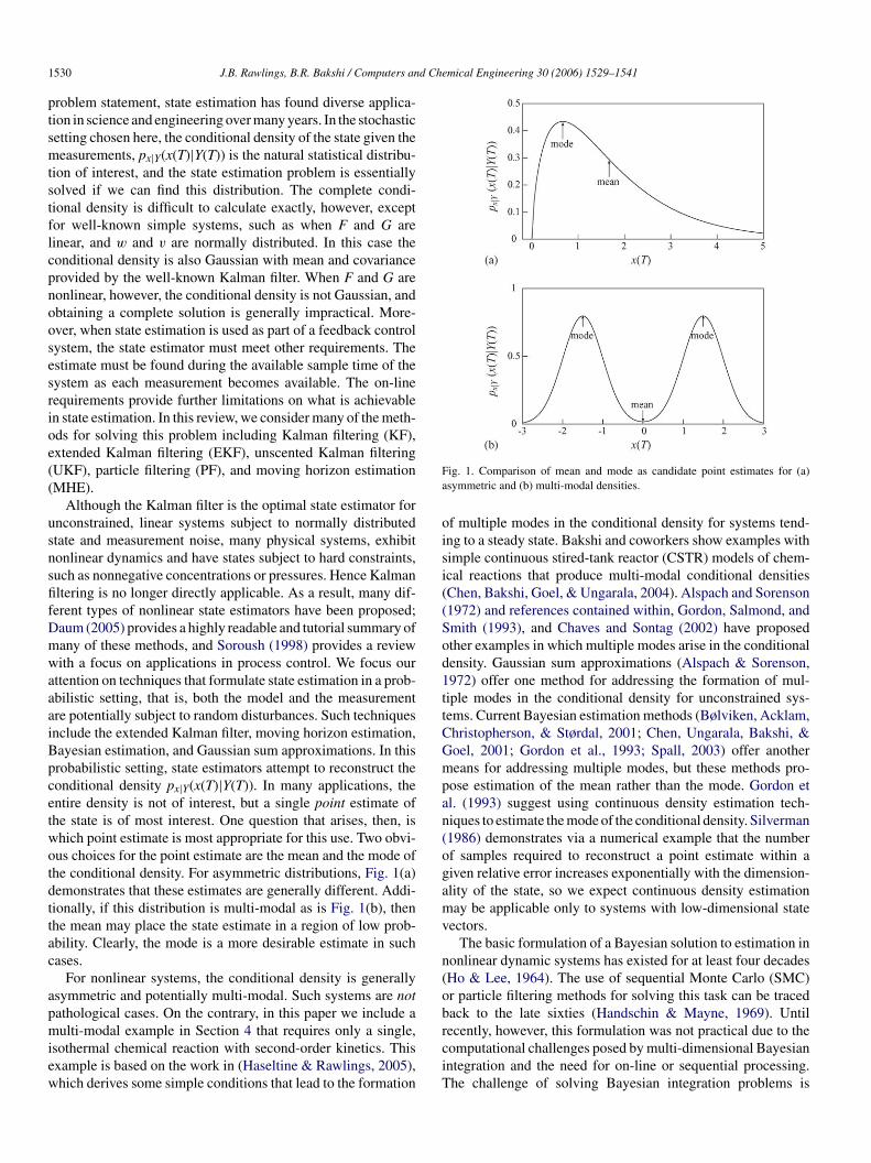
ttention on techniques that formulate state estimation in a prob-bilistic setting, that is, both the model and the measurementre potentially subject to random disturbances. Such techniquesnclude the extended Kalman filter, moving horizon estimation,ayesian estimation, and Gaussian sum approximations. In thisrobabilistic setting, state estimators attempt to reconstruct theonditional density px|Y(x(T)|Y(T)). In many applications, thentire density is not of interest, but a single point estimate ofhe state is of most interest. One question that arises, then, ishich point estimate is most appropriate for this use. Two obvi-us choices for the point estimate are the mean and the mode ofhe conditional density. For asymmetric distributions, Fig. 1(a)emonstrates that these estimates are generally different. Addi-ionally, if this distribution is multi-modal as is Fig. 1(b), thenhe mean may place the state estimate in a region of low prob-bility. Clearly, the mode is a more desirable estimate in suchases.

For nonlinear systems, the conditional density is generallysymmetric and potentially multi-modal. Such systems are notathological cases. On the contrary, in this paper we include a
ulti-modal example in Section 4 that requires only a single,
sothermal chemical reaction with second-order kinetics. Thisxample is based on the work in (Haseltine & Rawlings, 2005),hich derives some simple conditions that lead to the formation

rciT

ig. 1. Comparison of mean and mode as candidate point estimates for (a)symmetric and (b) multi-modal densities.

f multiple modes in the conditional density for systems tend-ng to a steady state. Bakshi and coworkers show examples withimple continuous stired-tank reactor (CSTR) models of chem-cal reactions that produce multi-modal conditional densitiesChen, Bakshi, Goel, & Ungarala, 2004). Alspach and Sorenson1972) and references contained within, Gordon, Salmond, andmith (1993), and Chaves and Sontag (2002) have proposedther examples in which multiple modes arise in the conditionalensity. Gaussian sum approximations (Alspach & Sorenson,972) offer one method for addressing the formation of mul-iple modes in the conditional density for unconstrained sys-ems. Current Bayesian estimation methods (Bølviken, Acklam,hristopherson, & Størdal, 2001; Chen, Ungarala, Bakshi, &oel, 2001; Gordon et al., 1993; Spall, 2003) offer anothereans for addressing multiple modes, but these methods pro-

ose estimation of the mean rather than the mode. Gordon etl. (1993) suggest using continuous density estimation tech-iques to estimate the mode of the conditional density. Silverman1986) demonstrates via a numerical example that the numberf samples required to reconstruct a point estimate within aiven relative error increases exponentially with the dimension-lity of the state, so we expect continuous density estimationay be applicable only to systems with low-dimensional state

ectors.The basic formulation of a Bayesian solution to estimation in

onlinear dynamic systems has existed for at least four decadesHo & Lee, 1964). The use of sequential Monte Carlo (SMC)r particle filtering methods for solving this task can be tracedack to the late sixties (Handschin & Mayne, 1969). Until
ecently, however, this formulation was not practical due to theomputational challenges posed by multi-dimensional Bayesianntegration and the need for on-line or sequential processing.he challenge of solving Bayesian integration problems is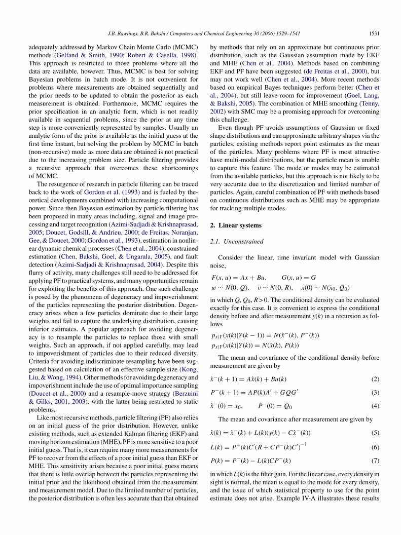

d Che

amTdBptmpasafi(dao

bopbc2GeedflafioewiawtCgLi(&p

oemiPMtiat

bdaEmba&2t

spohtfvpof

2

2

n

iedl

m

x

P

x

x

L

P

J.B. Rawlings, B.R. Bakshi / Computers an

dequately addressed by Markov Chain Monte Carlo (MCMC)ethods (Gelfand & Smith, 1990; Robert & Casella, 1998).his approach is restricted to those problems where all theata are available, however. Thus, MCMC is best for solvingayesian problems in batch mode. It is not convenient forroblems where measurements are obtained sequentially andhe prior needs to be updated to obtain the posterior as each

easurement is obtained. Furthermore, MCMC requires therior specification in an analytic form, which is not readilyvailable in sequential problems, since the prior at any timetep is more conveniently represented by samples. Usually annalytic form of the prior is available as the initial guess at therst time instant, but solving the problem by MCMC in batchnon-recursive) mode as more data are obtained is not practicalue to the increasing problem size. Particle filtering provides

recursive approach that overcomes these shortcomingsf MCMC.

The resurgence of research in particle filtering can be tracedack to the work of Gordon et al. (1993) and is fueled by the-retical developments combined with increasing computationalower. Since then Bayesian estimation by particle filtering haseen proposed in many areas including, signal and image pro-essing and target recognition (Azimi-Sadjadi & Krishnaprasad,005; Doucet, Godsill, & Andrieu, 2000; de Freitas, Noranjan,ee, & Doucet, 2000; Gordon et al., 1993), estimation in nonlin-

ar dynamic chemical processes (Chen et al., 2004), constrainedstimation (Chen, Bakshi, Goel, & Ungarala, 2005), and faultetection (Azimi-Sadjadi & Krishnaprasad, 2004). Despite thisurry of activity, many challenges still need to be addressed forpplying PF to practical systems, and many opportunities remainor exploiting the benefits of this approach. One such challenges posed by the phenomena of degeneracy and impoverishmentf the particles representing the posterior distribution. Degen-racy arises when a few particles dominate due to their largeeights and fail to capture the underlying distribution, causing

nferior estimates. A popular approach for avoiding degener-cy is to resample the particles to replace those with smalleights. Such an approach, if not applied carefully, may lead

o impoverishment of particles due to their reduced diversity.riteria for avoiding indiscriminate resampling have been sug-ested based on calculation of an effective sample size (Kong,iu, & Wong, 1994). Other methods for avoiding degeneracy and

mpoverishment include the use of optimal importance samplingDoucet et al., 2000) and a resample-move strategy (Berzuini

Gilks, 2001, 2003), with the latter being restricted to staticroblems.

Like most recursive methods, particle filtering (PF) also reliesn an initial guess of the prior distribution. However, unlikexisting methods, such as extended Kalman filtering (EKF) andoving horizon estimation (MHE), PF is more sensitive to a poor

nitial guess. That is, it can require many more measurements forF to recover from the effects of a poor initial guess than EKF orHE. This sensitivity arises because a poor initial guess means

hat there is little overlap between the particles representing thenitial prior and the likelihood obtained from the measurementnd measurement model. Due to the limited number of particles,he posterior distribution is often less accurate than that obtained

isae

mical Engineering 30 (2006) 1529–1541 1531

y methods that rely on an approximate but continuous prioristribution, such as the Gaussian assumption made by EKFnd MHE (Chen et al., 2004). Methods based on combiningKF and PF have been suggested (de Freitas et al., 2000), butay not work well (Chen et al., 2004). More recent methods

ased on empirical Bayes techniques perform better (Chen etl., 2004), but still leave room for improvement (Goel, Lang,

Bakshi, 2005). The combination of MHE smoothing (Tenny,002) with SMC may be a promising approach for overcominghis challenge.

Even though PF avoids assumptions of Gaussian or fixedhape distributions and can approximate arbitrary shapes via thearticles, existing methods report point estimates as the meanf the particles. Many problems where PF is most attractiveave multi-modal distributions, but the particle mean is unableo capture this feature. The mode or modes may be estimatedrom the available particles, but this approach is not likely to beery accurate due to the discretization and limited number ofarticles. Again, careful combination of PF with methods basedn continuous distributions such as MHE may be appropriateor tracking multiple modes.

. Linear systems

.1. Unconstrained

Consider the linear, time invariant model with Gaussianoise,

F (x, u) = Ax + Bu, G(x, u) = G

w ∼ N(0, Q), v ∼ N(0, R), x(0) ∼ N(x0, Q0)

n which Q, Q0, R > 0. The conditional density can be evaluatedxactly for this case. It is convenient to express the conditionalensity before and after measurement y(k) in a recursion as fol-ows

px|Y (x(k)|Y (k − 1)) = N(x−(k), P−(k))

px|Y (x(k)|Y (k)) = N(x(k), P(k))

The mean and covariance of the conditional density beforeeasurement are given by

ˆ−(k + 1) = Ax(k) + Bu(k) (2)

−(k + 1) = AP(k)A′ + GQG′ (3)

ˆ−(0) = x0, P−(0) = Q0 (4)

The mean and covariance after measurement are given by

ˆ(k) = x−(k) + L(k)(y(k) − Cx−(k)) (5)

(k) = P−(k)C′(R + CP−(k)C′)−1(6)

(k) = P−(k) − L(k)CP−(k) (7)

n which L(k) is the filter gain. For the linear case, every density inight is normal, the mean is equal to the mode for every density,nd the issue of which statistical property to use for the pointstimate does not arise. Example IV-A illustrates these results

1 d Che

ap

2

fsOta1mdTaaslcs

RascTmcob(bticbcuaihl

3

3

Ksfi

i

A

aG

tp(oidifiS(ameicm

vpada2

mee(

a

w


nd examines the performance of a particle filter on the sameroblem.

.2. Constrained

Constraints on thew(k),v(k), x(k) can be added to the problemormulation to refine the statistical description of the model. Thetatistical distribution of the noises are then truncated normals.ne may also use constraints to generate asymmetric distribu-

ions by piecing together truncated probability density functionss a jigsaw using variable decompositions (Robertson & Lee,995, 2002). The conditional densities are also truncated nor-als (Robertson & Lee, 2002). The modes of the conditional

ensity can be found by solving a convex quadratic program.he mean and mode of the conditional density are again equalnd the state estimate is uniquely defined. Because the densitiesre not multi-modal and a convex quadratic program (QP) can beolved to find the state estimate, the solution for the constrained,inear model is reasonably well in hand. Moreover, Bakshi andoworkers have recently proposed a PF method for treating con-trained systems (Chen et al., 2005).

As discussed in (Rao, 2000; Rao & Rawlings, 2002; Rao,awlings, & Mayne, 2003) care should be exercised whendding constraints to models used for state estimation. Con-traints on w(k) are not problematic. However, we advise againstonstraining v(k) due to the possibility of measurement outliers.hese constraints may amplify the effect of spurious measure-ents. Constraints on x(k) are nonstandard as well. One usually

hooses a model of the plant and, separately, the characteristicsf the disturbances, such as boundedness, or that the distur-ances are independent and identically distributed with knownzero) mean and variance. The properties of the model and distur-ances are distinct. State constraints, on the other hand, correlatehe disturbances with the state and may lead to acausality. If ones trying to enforce physical constraints, such as positivity ofoncentrations, for example, an alternative is to use a physicallyased nonlinear model that enforces the constraints automati-ally for all allowable x(0) and disturbance sequences. It remainsnclear if a simplified linear model with added state constraints isbetter choice than an appropriate nonlinear model that implic-

tly enforces the state constraints. This choice depends also onow well current state estimation methods can handle the non-inear model of interest.

. Nonlinear systems

.1. Extended Kalman filtering

The EKF linearizes the nonlinear system, then applies thealman filter to obtain the state estimates. The method can be

ummarized in a recursion similar in structure to the Kalman
lter (Stengel, 1994, 31, pp. 387–388)
x−(k + 1) = F (x(k), u(k))

P−(k + 1) = A(k)P(k)A′(k) + G(k)QG′(k)

x−(0) = x0, P−(0) = Q0

orttc

mical Engineering 30 (2006) 1529–1541

The mean and covariance after measurement are given by

x(k) = x−(k) + L(k)(y(k) − h(x−(k))

L(k) = P−(k)C′(k)(R + C(k)P−(k)C′(k))−1

P(k) = P−(k) − L(k)C(k)P−(k)

n which the following linearizations are made

¯ (k) = ∂F (x, u)

∂x, C(k) = ∂h(x)

∂x

nd all partial derivatives are evaluated at x(k) and u(k), and¯ (k) = G(x(k), u(k)). The densities of w, v and x0 are assumedo be normal. Many variations on the same theme have beenroposed such as the iterated EKF and the second-order EKFGelb, 1974, 32, 190–192). Of the nonlinear filtering meth-ds, the EKF method has received the most attention due tots relative simplicity and demonstrated effectiveness in han-ling some nonlinear systems. Examples of implementationsnclude estimation for the production of silicon/germanium alloylms (Middlebrooks, 2001), polymerization reactions (Prasad,chley, Russo, & Bequette, 2002), and fermentation processesGudi, Shah, & Gray, 1994). However, the EKF is at best and hoc solution to a difficult problem, and hence there existany pitfalls to the practical implementation of EKFs (see, for

xample, Wilson, Agarwal, & Rippin, 1998). These problemsnclude the inability to accurately incorporate physical stateonstraints and the naive use of linearization of the nonlinearodel.Until recently, few properties regarding the stability and con-

ergence of the EKF had been proven. Recent publicationsresent bounded estimation error and exponential convergencerguments for the continuous and discrete EKF forms givenetectability, small initial estimation error, small noise terms,nd no model error (Reif, Gunther, Yaz, & Unbehauen, 1999,000; Reif & Unbehauen, 1999).

However, depending on the system, the bounds on initial esti-ation error and noise terms may be unrealistic. Also, initial

stimation error may result in bounded estimate error but notxponential convergence, as illustrated by Chaves and Sontag2002).

Julier and Uhlmann (2004) summarize the status of the EKFs follows:

The extended Kalman filter is probably the most widely usedestimation algorithm for nonlinear systems. However, morethan 35 years of experience in the estimation community hasshown that it is difficult to implement, difficult to tune, and onlyreliable for systems that are almost linear on the time scale ofthe updates.

We seem to be making a transition from a previous era inhich new approaches to nonlinear filtering were criticized as
verly complex because “the EKF works,” to a new era in whichesearchers are demonstrating ever simpler examples in whichhe EKF fails completely. The unscented Kalman filter is one ofhe methods developed specifically to overcome the problemsaused by the naive linearization used in the EKF.

d Che

3

elpmtsubasUz

x

pamu

z

x

fiv

η

K

ip

wfp

DWo∂

(aBU

teIeeahsnTms

3

oota

i

m

p

c


.2. Unscented Kalman filtering

The linearization of the nonlinear model at the current statestimate may not accurately represent the dynamics of the non-inear system behavior even for one sample time. In the EKFrediction step, the mean propagates through the full nonlinearodel, but the covariance propagates through the lineariza-

ion. The resulting error is sufficient to throw off the correctiontep and the filter can diverge even with a perfect model. Thenscented Kalman filter avoids this linearization at a single pointy sampling the nonlinear response at several points. The pointsre called sigma points, and their locations and weights are cho-en to satisfy the given starting mean and covariance (Julier &hlmann, 2004a, 2004b).1 Given x and P, choose sample points,

i, and weights, wi, such that

ˆ =∑

i

wizi, P =∑

i

wi(zi − x)(zi − x)′

Similarly, given w N(0, Qw) and v N(0, Rv), choose sampleoints ni for w and mi for v. Each of the sigma points is prop-gated forward at each sample time using the nonlinear systemodel. The locations and weights of the transformed points then

pdate the mean and covariance.

i(k + 1) = F (zi(k), u(k)) + G(zi(k), u(k))ni(k), all i

From these we compute the forecast step

ˆ− =∑

i

wizi, P− =∑

i

wi(zi − x−)(zi − x−)′

After measurement, the EKF correction step is applied afterrst expressing this step in terms of the covariances of the inno-ation and state prediction

i = h(zi) + mi, y− =∑

i

wiηi

The output error is given as Y : y − y−. We next rewrite thealman filter update as

x = x− + L(y − y−)

L = E ((x − x−)Y′)︸︷︷︸P−C′

E (YY′)−1︸︷︷︸(R+CP−C′)−1

P = P− − LE ((x − x−)Y′)′︸︷︷︸CP−

n which we approximate the two expectations with the sigmaoint samples

− ′ ∑i i − i − ′
E ((x − x )Y ) ≈
i

w (z − x )(η − y )

E (YY′) ≈∑

i

wi(ηi − y−)(ηi − y−)′

1 Note that this idea is fundamentally different than the idea of particle filtering,hich is discussed subsequently. The sigma points are chosen deterministically,

or example as points on a selected covariance contour ellipse or a simplex. Thearticle filtering points are chosen by random sampling. p


See Julier and Uhlmann (2004a), Julier, Uhlmann, andurrant-Whyte (2000), van der Merwe, Doucet, de Freitas, andan (2000) for more details on the algorithm. An added benefit

f the UKF approach is that the partial derivatives ∂F(x,u)/∂x,h(x)/∂x are not required. See also Nørgaard, Poulsen, and Ravn2000) for other derivative-free nonlinear niters of comparableccuracy to the UKF. See (Julier & Uhlmann, 2002; Lefebvre,ruyninckx, & De Schutter, 2002) for an interpretation of theKF as a use of statistical linear regression.The UKF has been tested in a variety of simulation examples

aken from different application fields including aircraft attitudestimation, tracking and ballistics, and communication systems.n the chemical process control field, Romanenko and cowork-rs have compared the EKF and UKF on a strongly nonlinearxothermic chemical CSTR (Romanenko & Castro, 2004), andpH system (Romanenko, Santos, & Afonso, 2004). The CSTRas nonlinear dynamics and a linear measurement model, i.e. aubset of states is measured. In this case, the UKF performs sig-ificantly better than the EKF when the process noise is large.he pH system has linear dynamics but a strongly nonlineareasurement, i.e. the pH measurement. In this case, the authors

how a modest improvement in the UKF over the EKF.

.3. Full information estimation

Because the conditional density px|Y(x(T)|Y(T)) is difficult tobtain exactly for nonlinear models, we also focus our attentionn the entire trajectory of states X(T) := {x(0), . . . x(T)}, ratherhan just the last state x(T). For simplicity of presentation, wessume G = I in Eq. (1).

In the full information problem, Y(T) is available and our goals to find the maximum likelihood estimate by solving

axX(T )

pX|Y (X(T )|Y (T )) (8)

From Bayes theorem we have

X|Y (X(T )|Y (T )) = pY |X(Y (T )|X(T ))pX(X(T ))

pY (Y (T ))

Because the sequences w(k) and v(k) are independent, wean express the terms in the numerator as

pY |X(Y (T )|X(T )) =T∏

j=0

py|x(y(j)|x(j))

pX(X(T )) =T−1∏j=1

px|x(x(j + 1)|x(j))px(0)(x(0))

We also have

py|x(y(j)|x(j)) = pv(y(j) − h(x(j)))

px|x(x(j + 1)|x(j)) = pw(x(j + 1) − F (x(j), u(j)))

Substituting these results into Eq. (8), and noting thatY(Y(T)) does not depend on the decision variables X(T), the

1 d Che

m

t

X

s

ooWbtS

3

eMbLve

sctnrx

V

pttmt

ltMlp2

lotMt1D&RToZ

sRes1i(b&&rTeta(iMlcr

Mfat

(

(


aximum likelihood optimization is

maxX(T )

px(0)(x(0))T−1∏j=1

pw(x(j + 1) − F (x(j), u(j)))

×T∏

j=0

pv(y(j) − h(x(j)))

We can write this as an equivalent minimization problem byaking the negative logarithm to yield

min(T )

V0(x(0)) +T−1∑j=1

Lw(w(j)) +T∑

j=0

Lv(y(j) − h(x(j))) (9)

ubject to x(j + 1) = F (x(j), u(j)) + w(j) in which

V0(x):= − log(px(0)(x))

Lw(w):= − log(pw(w)), Lv(v):= − log(pv(v))

If the three densities above are chosen as normals, then webtain a nonlinear least-squares problem (nonlinear becausef the model constraint), but any given densities are allowed.e often default to using normals in applications solely

ecause of lack of knowledge about the densities of the ini-ial state and the disturbances. This issue is discussed briefly inection 3.6.

.4. Moving horizon estimation

The computational burden of solving the full informationstimator, Eq. (9), grows as measurements become available.oving horizon estimation (MHE) fixes this computational cost

y considering a finite horizon of only the last N measurements.et X(T − N: T) := {x(T − N) . . . x(T)} denote the most recent Nalues of the state sequence at current time T. The MHE statestimation problem is

minX(T−N:T )

VT−N (x(T − N)) +T−1∑

j=T−N

Lw(w(j))

+T∑

j=T−N

Lv(y(j) − h(x(j))) (10)

ubject to x(j + 1) = F (x(j), u(j)) + w(j) in which VT−N isalled the arrival cost. The arrival cost represents the informa-ion in the prior measurement sequence Y(T − N − 1) that isot considered in the horizon at time T. The statistically cor-ect choice for the arrival cost is the conditional density of(T − N)|Y(T − N − 1)

T−N (x) = −log px(T−N)|Y (x|Y (T − N − 1))

In the linear, Gaussian case, this conditional density is sim-ly P−(T − N), and MHE reduces exactly to the Kalman filter. In
he nonlinear case, this density is not available (or we can solvehe full information problem). We therefore consider various
ethods for approximating it. One option is to use a lineariza-ion approximation as in the EKF. Note that with a reasonably

lfe


arge value of N, MHE based on the EKF arrival cost is nothe same as the EKF. Numerous simulation examples show that

HE’s fitting the data in the horizon and using the full non-inear model in the state equation provides robustness to poorriors that is not achievable with the EKF (Haseltine & Rawlings,005).

The full information or MHE optimization approaches haveong been used in the process control community as meth-ds of state estimation, data reconciliation, and fault detec-ion for nonlinear models: Joseph, Edgar, Bequette, Biegler,

arquardt, Doyle and coworkers have proposed variations ofhis general approach (Albuquerque & Biegler, 1996; Bequette,991; Binder, Blank, Dahmen, & Marquardt, 2002; Gatzke &oyle, 2002; Kim, Liebman, & Edgar, 1991; Liebman, Edgar,Lasdon, 1992; M’hamdi, Helbig, Abel, & Marquardt, 1996;

amamurthi, Sistu, & Bequette, 1993; Tjoa & Biegler, 1991).hese approaches have also been used for designing nonlinearbservers (Michalska & Mayne, 1995; Moraal & Grizzle, 1995;immer, 1994).

The stability of MHE for constrained linear systems has beentudied for linear and nonlinear models (Meadows, Muske, &awlings, 1993; Muske & Rawlings, 1995) Statistical prop-rties of constrained linear and nonlinear MHE have beentudied by Robertson and Lee (Robertson, Lee, & Rawlings,996; Robertson & Lee, 2002) Tyler and Morari have exam-ned the feasibility issue for constrained MHE for linear modelsTyler & Morari, 1996). Rao et al. have worked on the sta-ility of linear and nonlinear, constrained MHE (Michalska

Mayne, 1995; Rao & Rawlings, 2000; Rao, Rawlings,Lee, 2001; Rao et al., 2003). Ferrari-Trecate et al. have

ecently extended MHE for use with hybrid systems (Ferrari-recate, Mignone, & Morari, 2002). Goodwin and cowork-rs have shown a nice duality between constrained estima-ion and control (Goodwin, De Dona, Seron, & Zhuo, 2005)nd also designed MHE for distributed, networked systemsGoodwin, Haimovich, Quevedo, & Welsh, 2005). Advancesn numerical optimization have made it possible to solve the

HE optimization in real time for small dimensional non-inear models (Tenny & Rawlings, 2002). But computationalomplexity remains a significant research challenge for MHEesearchers.

The best choice of arrival cost remains an open issue inHE research. Rao et al. (2001) explore estimating this cost

or constrained linear systems with the corresponding cost forn unconstrained linear system. More specifically, the followingwo schemes are examined:

1) a “filtering” scheme that penalizes deviations of the initialestimate in the horizon from a prior estimate, and

2) a “smoothing” scheme that penalizes deviations of the tra-jectory of states in the estimation horizon from a priorestimate.

For unconstrained, linear systems, the MHE optimization col-apses to the Kalman filter for both of these schemes. Rao (2000)urther considers several optimal and suboptimal approaches forstimating the arrival cost via a series of optimizations. These

d Che

atsOict

tsaTfitislmRwoialc

3

tsv

p

iiTcatlibal

p

f

iTa

p

iLt

p

ttmYse

E

daq

E

i

q

iistaiothe

(pcthe particles and weights, (xi(T − 1), qi(T − 1)), which repre-


pproaches stem from the property that, in a deterministic set-ing (no state or measurement noise), MHE is an asymptoticallytable observer as long as the arrival cost is underbounded.ne simple way of estimating the arrival cost, therefore, is to

mplement a uniform prior. Computationally, a uniform priororresponds to not penalizing deviations of the initial state fromhe prior estimate.

For nonlinear systems, Tenny and Rawlings (2002) estimatehe arrival cost by approximating the constrained, nonlinearystem as an unconstrained, linear time-varying system andpplying the corresponding filtering and smoothing schemes.hey conclude that the smoothing scheme is superior to theltering scheme because the filtering scheme induces oscilla-

ions in the state estimates due to unnecessary propagation ofnitial error. The assumption here is that the conditional den-ity is well approximated by a multivariate normal. The prob-em with this assumption of course is that nonlinear systems

ay exhibit a multi-modal conditional density. Haseltine andawlings (2002) demonstrate that approximating the arrival costith the smoothing scheme in the presence of multiple localptima may skew all future estimates. If global optimization ismplementable in real time, approximating the arrival cost withuniform prior and making the estimation horizon reasonably

ong is preferable to an approximate multivariate normal arrivalost.

.5. Particle filtering

Unlike most other nonlinear filtering methods, includinghose described earlier, particle filtering does not assume a fixedhape of any density, but approximates the densities of interestia samples or particles

(x(t)) ≈np∑i=1

qi(t)δ(x(t) − xi(t))

n which np is the number of particles or samples in the approx-mation, xi is the sample location and qi is the sample weight.hus PF can capture the time-varying nature of distributionsommonly encountered in nonlinear dynamic problems, andny moment can be calculated from the samples. Furthermore,his sampling based approach can solve the estimation prob-em in a recursive manner without resorting to model approx-mation. The posterior at time T may be written recursivelyased on prior knowledge of the system, px|Y(x(T)|Y(T − 1)),nd the current information of the process, py|x(y(T)|x(T)) orikelihood

x|Y (x(T )|Y (T )) ∝ py|x(y(T )|x(T ))px|Y (x(T )|Y (T − 1)) (11)

The two terms on the right hand side of Eq. (11) may beurther manipulated as follows.

px|Y (x(T )|Y (T − 1))

=∫

px|x(x(T )|x(T − 1))px|Y (x(T − 1)|Y (T − 1)) dx(T − 1)

(12)

srtt


n which p(x(T − 1)|Y(T − 1)) is the posterior at time step T − 1.he distribution of px|x(x(T)|x(T − 1)) can be found based on thevailable state equation, Eq. (1), as,

x|x(x(T )|x(T − 1)) =∫

δ(x(T ) − f (x(T − 1), w(T − 1)))

× pw(w(T − 1)) dw(T − 1) (13)

n which we use the notation f (x, w):=F (x, u) + G(x, u)w.ikewise the likelihood distribution can be expressed based on

he measurement equation, Eq. (1), as follows,

y|x(y(T )|x(T )) =∫

δ(y(T ) − h(x(T ), v(T )))pv(v(T )) dv(T )

(14)

Using Monte Carlo sampling for solving the dynamic estima-ion problem requires an approach for generating samples fromhe posterior at each time point, while incorporating the state and

easurement equations, Eq. (1), and available measurements,(T). This may be accomplished via sequential Monte Carloampling with Eqs. (11)–(14) followed by using the followingquation for calculating the posterior moments.

[f (x)] =∫

f (x)p(x) dx ≈ 1

N

N∑i=1

f (xi) (15)

Eq. (15) requires samples from the posterior, which are oftenifficult to obtain since the posterior may have unusual shapesnd may lack a convenient closed-form representation. Conse-uently, it is common to write Eq. (15) as,

[f (x)] =∫

f (x)p(x)

π(x)π(x) dx ≈ 1

N

N∑i=1

f (xi)f (xi)qi (16)

n which

i = p(xi)

π(xi)(17)

s the weight function and {xi} are samples drawn from themportance function, π(x). This formulation permits convenientampling from a known distribution, π(x), and relaxes the needo draw samples from the true posterior distribution, p(x). Also,ny pairs of samples (particles) and weights, {xi, qi} containnformation about the relevant distribution. A basic requirementf the importance function is that its support should includehe support of the true distribution (Geweke, 1989). Moreover,aving f(xi)q(xi) roughly equal for all particles ensures precisestimates.

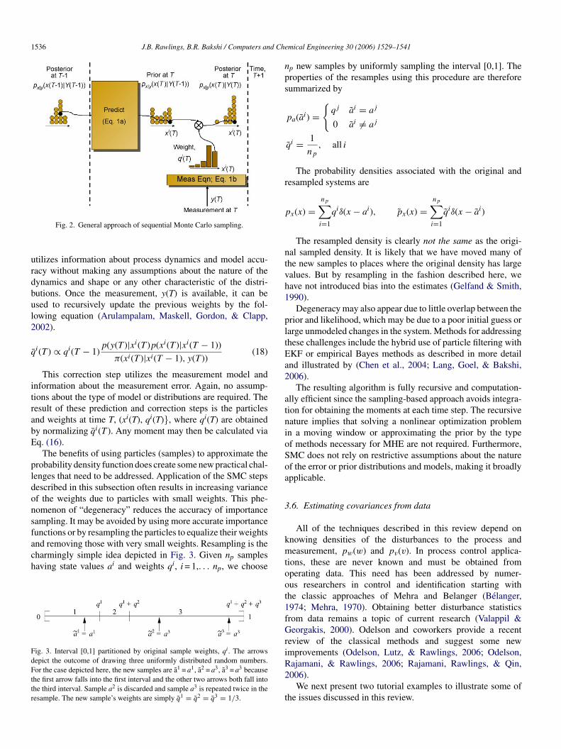
A computationally efficient and recursive solution to Eqs.12)–(14) is provided by sequential Monte Carlo (SMC) sam-ling. The recursive approach of SMC is depicted graphi-ally in Fig. 2. Information available at time T − 1 includes

ent the posterior at time T − 1, px|Y(x(T − 1)|Y(T − 1)). Bayesule is applied recursively by passing each sample throughhe state equation, Eq. (1), to obtain samples correspondingo the prior at time T, px|Y(x(T)|Y(T − 1)). This prediction step

1536 J.B. Rawlings, B.R. Bakshi / Computers and Che

urdbul2

q

itrabE

pldonsfach

FdFttr

nps

r

p

ntvh1

pltEa2

atnioSoa

3

Fig. 2. General approach of sequential Monte Carlo sampling.

tilizes information about process dynamics and model accu-acy without making any assumptions about the nature of theynamics and shape or any other characteristic of the distri-utions. Once the measurement, y(T) is available, it can besed to recursively update the previous weights by the fol-owing equation (Arulampalam, Maskell, Gordon, & Clapp,002).

¯ i(T ) ∝ qi(T − 1)p(y(T )|xi(T )p(xi(T )|xi(T − 1))

π(xi(T )|xi(T − 1), y(T ))(18)

This correction step utilizes the measurement model andnformation about the measurement error. Again, no assump-ions about the type of model or distributions are required. Theesult of these prediction and correction steps is the particlesnd weights at time T, (xi(T), qi(T)}, where qi(T) are obtainedy normalizing qi(T ). Any moment may then be calculated viaq. (16).

The benefits of using particles (samples) to approximate therobability density function does create some new practical chal-enges that need to be addressed. Application of the SMC stepsescribed in this subsection often results in increasing variancef the weights due to particles with small weights. This phe-omenon of “degeneracy” reduces the accuracy of importanceampling. It may be avoided by using more accurate importance
unctions or by resampling the particles to equalize their weightsnd removing those with very small weights. Resampling is theharmingly simple idea depicted in Fig. 3. Given np samplesaving state values ai and weights qi, i = 1,. . . np, we choose
ig. 3. Interval [0,1] partitioned by original sample weights, qi. The arrowsepict the outcome of drawing three uniformly distributed random numbers.or the case depicted here, the new samples are a1 = a1, a2 = a3, a3 = a3 because

he first arrow falls into the first interval and the other two arrows both fall intohe third interval. Sample a2 is discarded and sample a3 is repeated twice in theesample. The new sample’s weights are simply q1 = q2 = q3 = 1/3.

kmtoot1fGriR2

t


p new samples by uniformly sampling the interval [0,1]. Theroperties of the resamples using this procedure are thereforeummarized by

pa(ai) ={

qj ai = aj

0 ai �= aj

qi = 1

np

, all i

The probability densities associated with the original andesampled systems are

x(x) =np∑i=1

qiδ(x − ai), px(x) =np∑i=1

qiδ(x − ai)

The resampled density is clearly not the same as the origi-al sampled density. It is likely that we have moved many ofhe new samples to places where the original density has largealues. But by resampling in the fashion described here, weave not introduced bias into the estimates (Gelfand & Smith,990).

Degeneracy may also appear due to little overlap between therior and likelihood, which may be due to a poor initial guess orarge unmodeled changes in the system. Methods for addressinghese challenges include the hybrid use of particle filtering withKF or empirical Bayes methods as described in more detailnd illustrated by (Chen et al., 2004; Lang, Goel, & Bakshi,006).

The resulting algorithm is fully recursive and computation-lly efficient since the sampling-based approach avoids integra-ion for obtaining the moments at each time step. The recursiveature implies that solving a nonlinear optimization problemn a moving window or approximating the prior by the typef methods necessary for MHE are not required. Furthermore,MC does not rely on restrictive assumptions about the naturef the error or prior distributions and models, making it broadlypplicable.

.6. Estimating covariances from data

All of the techniques described in this review depend onnowing densities of the disturbances to the process andeasurement, pw(w) and pv(v). In process control applica-

ions, these are never known and must be obtained fromperating data. This need has been addressed by numer-us researchers in control and identification starting withhe classic approaches of Mehra and Belanger (Belanger,974; Mehra, 1970). Obtaining better disturbance statisticsrom data remains a topic of current research (Valappil &eorgakis, 2000). Odelson and coworkers provide a recent

eview of the classical methods and suggest some newmprovements (Odelson, Lutz, & Rawlings, 2006; Odelson,
ajamani, & Rawlings, 2006; Rajamani, Rawlings, & Qin,006).
We next present two tutorial examples to illustrate some ofhe issues discussed in this review.

J.B. Rawlings, B.R. Bakshi / Computers and Chemical Engineering 30 (2006) 1529–1541 1537

Fm

4

4

icx

osds

acEabs

natafi

Fig. 5. Particle locations vs. time; 500 particles.

F5

isedIttorder of hundreds of states compared to this two-state tutorialexample.

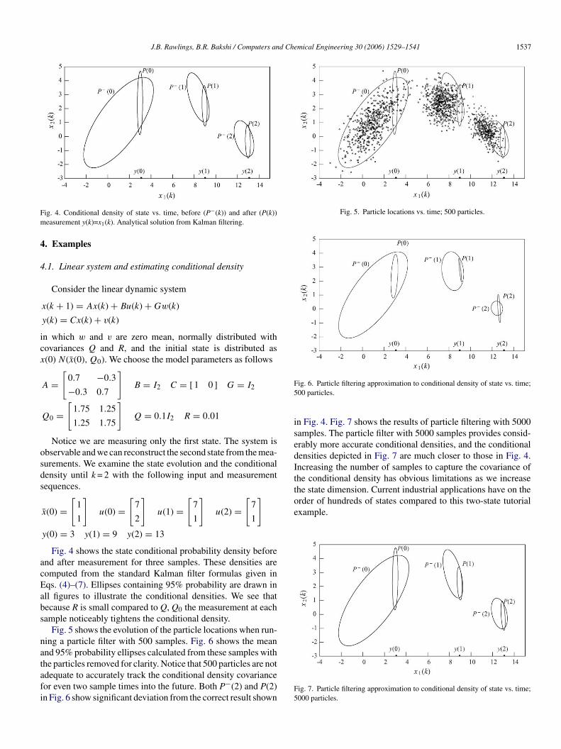
ig. 4. Conditional density of state vs. time, before (P−(k)) and after (P(k))easurement y(k)=x1(k). Analytical solution from Kalman filtering.

. Examples

.1. Linear system and estimating conditional density

Consider the linear dynamic system

x(k + 1) = Ax(k) + Bu(k) + Gw(k)

y(k) = Cx(k) + v(k)

n which w and v are zero mean, normally distributed withovariances Q and R, and the initial state is distributed as(0) N(x(0), Q0). We choose the model parameters as follows

A =[

0.7 −0.3

−0.3 0.7

]B = I2 C = [ 1 0 ] G = I2

Q0 =[

1.75 1.25

1.25 1.75

]Q = 0.1I2 R = 0.01

Notice we are measuring only the first state. The system isbservable and we can reconstruct the second state from the mea-urements. We examine the state evolution and the conditionalensity until k = 2 with the following input and measurementequences.

x(0) =[

1

1

]u(0) =

[7

2

]u(1) =

[7

1

]u(2) =

[7

1

]y(0) = 3 y(1) = 9 y(2) = 13

Fig. 4 shows the state conditional probability density beforend after measurement for three samples. These densities areomputed from the standard Kalman filter formulas given inqs. (4)–(7). Ellipses containing 95% probability are drawn inll figures to illustrate the conditional densities. We see thatecause R is small compared to Q, Q0 the measurement at eachample noticeably tightens the conditional density.

Fig. 5 shows the evolution of the particle locations when run-ing a particle filter with 500 samples. Fig. 6 shows the meannd 95% probability ellipses calculated from these samples with
he particles removed for clarity. Notice that 500 particles are notdequate to accurately track the conditional density covarianceor even two sample times into the future. Both P−(2) and P(2)n Fig. 6 show significant deviation from the correct result shown
F5

ig. 6. Particle filtering approximation to conditional density of state vs. time;00 particles.

n Fig. 4. Fig. 7 shows the results of particle filtering with 5000amples. The particle filter with 5000 samples provides consid-rably more accurate conditional densities, and the conditionalensities depicted in Fig. 7 are much closer to those in Fig. 4.ncreasing the number of samples to capture the covariance ofhe conditional density has obvious limitations as we increasehe state dimension. Current industrial applications have on the

ig. 7. Particle filtering approximation to conditional density of state vs. time;000 particles.

1538 J.B. Rawlings, B.R. Bakshi / Computers and Chemical Engineering 30 (2006) 1529–1541

ficmTndooNoBamiocldms

4

2

si

x

sQc

pP

Fb

RtQtc

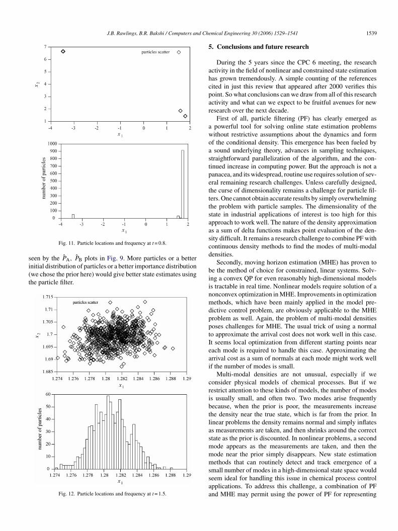
btaiat time t = 0.8 in Fig. 11. The multiple peaks finally disappearat time t = 1.5 as seen in Fig. 12. The mean estimate using theparticle filter does not converge to the actual state, however, as

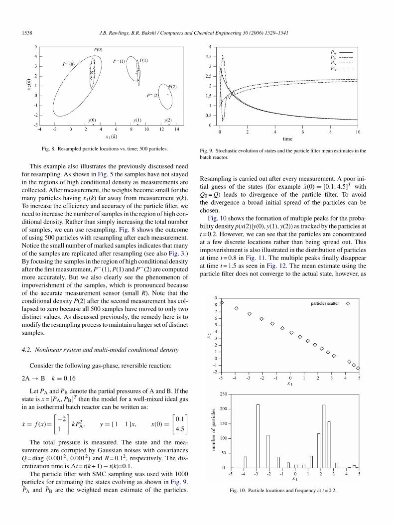
Fig. 8. Resampled particle locations vs. time; 500 particles.

This example also illustrates the previously discussed needor resampling. As shown in Fig. 5 the samples have not stayedn the regions of high conditional density as measurements areollected. After measurement, the weights become small for theany particles having x1(k) far away from measurement y(k).o increase the efficiency and accuracy of the particle filter, weeed to increase the number of samples in the region of high con-itional density. Rather than simply increasing the total numberf samples, we can use resampling. Fig. 8 shows the outcomef using 500 particles with resampling after each measurement.otice the small number of marked samples indicates that manyf the samples are replicated after resampling (see also Fig. 3.)y focusing the samples in the region of high conditional densityfter the first measurement, P−(1), P(1) and P−(2) are computedore accurately. But we also clearly see the phenomenon of

mpoverishment of the samples, which is pronounced becausef the accurate measurement sensor (small R). Note that theonditional density P(2) after the second measurement has col-apsed to zero because all 500 samples have moved to only twoistinct values. As discussed previously, the remedy here is toodify the resampling process to maintain a larger set of distinct

amples.

.2. Nonlinear system and multi-modal conditional density

Consider the following gas-phase, reversible reaction:

A → B k = 0.16

Let PA and PB denote the partial pressures of A and B. If thetate is x = [PA, PB]T then the model for a well-mixed ideal gasn an isothermal batch reactor can be written as:

˙ = f (x)=[

−2

1

]kP2

A, y = [ 1 1 ]x, x(0) =[

0.1

4.5

]

The total pressure is measured. The state and the mea-urements are corrupted by Gaussian noises with covariances= diag (0.0012, 0.0012) and R = 0.12, respectively. The dis-

retization time is �t = t(k + 1) − t(k)=0.1.The particle filter with SMC sampling was used with 1000

articles for estimating the states evolving as shown in Fig. 9.ˆ A and PB are the weighted mean estimate of the particles.

ig. 9. Stochastic evolution of states and the particle filter mean estimates in theatch reactor.

esampling is carried out after every measurement. A poor ini-ial guess of the states (for example x(0) = [0.1, 4.5]T with

0 = Q) leads to divergence of the particle filter. To avoidhe divergence a broad initial spread of the particles can behosen.

Fig. 10 shows the formation of multiple peaks for the proba-ility density p(x(2)|y(0), y(1), y(2)) as tracked by the particles at= 0.2. However, we can see that the particles are concentratedt a few discrete locations rather than being spread out. Thismpoverishment is also illustrated in the distribution of particles

Fig. 10. Particle locations and frequency at t = 0.2.

J.B. Rawlings, B.R. Bakshi / Computers and Che

si(t

5

ahcpar

awoastpetttsaascd


ˆ ˆ
een by the PA, PB plots in Fig. 9. More particles or a betternitial distribution of particles or a better importance distributionwe chose the prior here) would give better state estimates usinghe particle filter.

biinmdpptIeai

cribtlasmmmssaa


. Conclusions and future research

During the 5 years since the CPC 6 meeting, the researchctivity in the field of nonlinear and constrained state estimationas grown tremendously. A simple counting of the referencesited in just this review that appeared after 2000 verifies thisoint. So what conclusions can we draw from all of this researchctivity and what can we expect to be fruitful avenues for newesearch over the next decade.

First of all, particle filtering (PF) has clearly emerged aspowerful tool for solving online state estimation problemsithout restrictive assumptions about the dynamics and formf the conditional density. This emergence has been fueled bysound underlying theory, advances in sampling techniques,

traightforward parallelization of the algorithm, and the con-inued increase in computing power. But the approach is not aanacea, and its widespread, routine use requires solution of sev-ral remaining research challenges. Unless carefully designed,he curse of dimensionality remains a challenge for particle fil-ers. One cannot obtain accurate results by simply overwhelminghe problem with particle samples. The dimensionality of thetate in industrial applications of interest is too high for thispproach to work well. The nature of the density approximations a sum of delta functions makes point evaluation of the den-ity difficult. It remains a research challenge to combine PF withontinuous density methods to find the modes of multi-modalensities.

Secondly, moving horizon estimation (MHE) has proven toe the method of choice for constrained, linear systems. Solv-ng a convex QP for even reasonably high-dimensional modelss tractable in real time. Nonlinear models require solution of aonconvex optimization in MHE. Improvements in optimizationethods, which have been mainly applied in the model pre-

ictive control problem, are obviously applicable to the MHEroblem as well. Again, the problem of multi-modal densitiesoses challenges for MHE. The usual trick of using a normalo approximate the arrival cost does not work well in this case.t seems local optimization from different starting points nearach mode is required to handle this case. Approximating therrival cost as a sum of normals at each mode might work wellf the number of modes is small.

Multi-modal densities are not unusual, especially if weonsider physical models of chemical processes. But if weestrict attention to these kinds of models, the number of modess usually small, and often two. Two modes arise frequentlyecause, when the prior is poor, the measurements increasehe density near the true state, which is far from the prior. Ininear problems the density remains normal and simply inflatess measurements are taken, and then shrinks around the correcttate as the prior is discounted. In nonlinear problems, a secondode appears as the measurements are taken, and then theode near the prior simply disappears. New state estimationethods that can routinely detect and track emergence of a

mall number of modes in a high-dimensional state space wouldeem ideal for handling this issue in chemical process controlpplications. To address this challenge, a combination of PFnd MHE may permit using the power of PF for representing

1 d Che

ta

A

tptAN

R

A

A

A

A

A

B

B

B

B

B

B

C

C

C

C

D

d

D

F

G

G

G

G

G

G

G

G

G

H

H

H

H

J

J

J

J

K

K

L


he general, multi-modal densities, and the power of MHE forccurately tracking the locations of the modes.

cknowledgments

The authors would like to thank M. Rajamani, E.L. Hasel-ine, and D.Q. Mayne for helpful discussion of the ideas in thisaper. The first author acknowledges financial support from NSFhrough grant #CNS-0540147 and PRF through grant #43321-C9. The second author acknowledges financial support fromSF through grant #CTS-0321911.

eferences

lbuquerque, J., & Biegler, L. T. (1996). Data reconciliation and gross-errordetection for dynamic systems. AIChE Journal, 42(10), 2841–2856.

lspach, D. L., & Sorenson, H. W. (1972). Nonlinear Bayesian estimation usingGaussian sum approximations. IEEE Transactions on Automatic Control,AC-17(4), 439–448.

rulampalam, M. S., Maskell, S., Gordon, N., & Clapp, T. (2002, Febru-ary). A tutorial on particle filters for online nonlinear/non-GaussianBayesian tracking. IEEE Transactions on Signal Processing, 50(2), 174–188.

zimi-Sadjadi, B., & Krishnaprasad, P. S. (2004). “A particle filtering approachto change detection for nonlinear systems,” Rensselaer Polytechnic Institute,Tech. Rep. Submitted to EURASIP Journal on Applied Signal Processing(EURASIP JASP).

zimi-Sadjadi, B., & Krishnaprasad, P. (2005). Approximate nonlinear filteringand its application in navigation. Automatica, 41(6), 945–956.

elanger, P. (1974). Estimation of noise covariance matrices for a linear time-varying stochastic process. Automatica, 10, 267–275.

equette, B. W. (1991, February). Nonlinear predictive control using multi-rate sampling. Canadian Journal of Chemical Engineering, 69, 136–143.

erzuini, C., & Gilks, W. (2001). Resample-move filtering with cross-modeljumps. In A. Doucet, N. de Freitas, & N. Gordon (Eds.), Sequential MonteCarlo methods in practice (pp. 117–138). New York: Springer.

erzuini, C., & Gilks, W. R. (2003). Particle filtering methods for dynamicand static Bayesian problems. In P. J. Green, N. L. Hjort, & S. Richardson(Eds.), Highly structured stochastic systems (pp. 207–236). Oxford: OxfordUniversity Press.

inder, T., Blank, L., Dahmen, W., & Marquardt, W. (2002). On the regulariza-tion of dynamic data reconciliation problems. Journal of Process Control,12(4), 557–567.

ølviken, E., Acklam, P. J., Christopherson, N., & Størdal, J.-M. (2001, Febru-ary). Monte Carlo filters for non-linear state estimation. Automatica, 37(2),177–183.

haves, M., & Sontag, E. (2002). State-estimators for chemical reaction net-works of Feinberg-Horn-Jackson zero deficiency type. European Journal ofControl, 8(4), 343–359.

hen, W. S., Bakshi, B. R., Goel, P. K., & Ungarala, S. (2004). Bayesian esti-mation of unconstrained nonlinear dynamic systems via sequential MonteCarlo sampling. Industrial and Engineering Chemistry Research, 43(14),4012–4025.

hen, W. S., Bakshi, B. R., Goel, P. K., & Ungarala, S. (2005). “Bayesianestimation of constrained nonlinear dynamic systems via sequential MonteCarlo sampling,” Submitted to Automatica.

hen, W. S., Ungarala, S., Bakshi, B., & Goel, P. (2001). “Bayesian rectificationof nonlinear dynamic processes by the weighted bootstrap,” in AIChE AnnualMeeting, Reno, Nevada.

aum, F. (2005, August). Nonlinear filters: Beyond the Kalman filter. IEEEA&E Systems Magazine, 20(8), 57–69, Part 2: Tutorials.

e Freitas, J. F. G., Noranjan, M., Gee, A. H., & Doucet, A. (2000). SequentialMonte Carlo methods to train neural network models. Neural Computation,12, 955–993.

L


oucet, A., Godsill, S., & Andrieu, C. (2000). On sequential Monte Carlo sam-pling methods for Bayesian filtering. Statistics and Computing, 10, 197–208.

errari-Trecate, G., Mignone, D., & Morari, M. (2002). Moving horizon estima-tion for hybrid systems. IEEE Transactions on Automatic Control, 47(10),1663–1676.

atzke, E., & Doyle, F. J. (2002). Use of multiple models and qualitative knowl-edge for on-line moving horizon disturbance estimation and fault diagnosis.Journal of Process Control, 12(2), 339–352.

elb, A. (Ed.). (1974). Applied optimal estimation. Cambridge, Massachusetts:The M.I.T. Press.

elfand, A., & Smith, A. (1990). Sampling based approaches to calculatingmarginal densities. Journal of the American Statistical Association, 85,398–408.

eweke, J. (1989, November). Bayesian inference in econometric models usingMonte Carlo integration. Econometrica, 57(6), 1317–1339.

oel, P., Lang, L., & Bakshi, B. R. (2005, January). Sequential Monte Carloin Bayesian inference for dynamic models: An overview. In Proceedings ofInternational Workshop/Conference on Bayesian Statistics and its Applica-tions, Co-sponsored by International Society for Bayesian Analysis.

oodwin, G. C., De Dona, J. A., Seron, M. A., & Zhuo, X. W. (2005).Lagrangian duality between constrained estimation and control. Automat-ica, 41, 935–944.

oodwin, G. C., Haimovich, H., Quevedo, D. E., & Welsh, J. S. (2005, Septem-ber). A moving horizon approach to networked control system design. IEEETransactions on Automatic Control, 49(9), 1427–1445.

ordon, N., Salmond, D., & Smith, A. (1993, April). Novel approach tononlinear/non-Gaussian Bayesian state estimation. IEE Proceedings F-Radar and Signal Processing, 140(2), 107–113.

udi, R., Shah, S., & Gray, M. (1994). Multirate state and parameter estimationin an antibiotic fermentation with delayed measurements. Biotechnology andBioengineering, 44, 1271–1278.

andschin, J. E., & Mayne, D. Q. (1969). Monte Carlo techniques to estimatethe conditional expectation in multistage nonlinear filtering. InternationalJournal of Control, 9(5), 547–559.

aseltine, E. L., & Rawlings, J. B. (2002). “A critical evaluation of extendedKalman filtering and moving horizon estimation,” TWMCC, Departmentof Chemical Engineering, University of Wisconsin-Madison, Tech. Rep.2002–03, August 2002.

aseltine, E. L., & Rawlings, J. B. (2005, April). Critical evaluation ofextended Kalman filtering and moving horizon estimation. Industrial andEngineering Chemistry Research, 44(8), 2451–2460 [Online]. Available:http://pubs.acs.org/journals/iecred/.

o, Y. C., & Lee, R. C. K. (1964). A Bayesian approach to problems in stochas-tic estimation and control. IEEE Transactions on Automatic Control, 9(5),333–339.

ulier, S., & Uhlmann, J. (2002, August). Author’s reply. IEEE Transactions onAutomatic Control, 47(8), 1408–1409.

ulier, S. J., & Uhlmann, J. K. (2004, March). Unscented filtering and nonlinearestimation. Proceedings of the IEEE, 92(3), 401–422.

ulier, S. J., & Uhlmann, J. K. (2004, December). Corrections to unscentedfiltering and nonlinear estimation. Proceedings of the IEEE, 92(12), 1958.

ulier, S. J., Uhlmann, J. K., & Durrant-Whyte, H. F. (2000, March). Anew method for the nonlinear transformation of means and covariancesin filters and estimators. IEEE Transactions on Automatic Control, 45(3),477–482.

im, I., Liebman, M., & Edgar, T. (1991). A sequential error-in-variablesmethod for nonlinear dynamic systems. Computers and Chemical Engineer-ing, 15(9), 663–670.

ong, A., Liu, J. S., & Wong, W. H. (1994, March). Sequential imputationsand Bayesian missing data problems. Journal of the American StatisticalAssociation, 89(425), 278–288.

ang, L., Goel, P. K., & Bakshi, B. R. (2006, January). A smoothing basedmethod to improve performance of sequential Monte Carlo estimation under
poor initial guess. In Proceedings of Chemical Process Control 7.
efebvre, T., Bruyninckx, H., & De Schutter, J. (2002, August). Comment on“A new method for the nonlinear transformation of means and covariancesin filters and estimators. IEEE Transactions on Automatic Control, 47(8),1406–1408.

d Che

L

M

M

M

M

M

M

M

N

O

O

P

R

R

R

R

R

R

R

R

R

R

R

R

R

R

R

R

S

S

S

ST

T

T

T

V

v


iebman, M., Edgar, T., & Lasdon, L. (1992). Efficient data reconcilia-tion and estimation for dynamic processes using nonlinear program-ming techniques. Computers and Chemical Engineering, 16(10/11), 963–986.

eadows, E. S., Muske, K. R., & Rawlings, J. B. (1993, June). Constrainedstate estimation and discontinuous feedback in model predictive control. InProceedings of the 1993 European Control Conference (pp. 2308–2312).

ehra, R. (1970). On the identification of variances and adaptive Kalman filter-ing. IEEE Transactions on Automatic Control, 15(12), 175–184.

’hamdi, A., Helbig, A., Abel, O., & Marquardt, W. (1996). Newton-type reced-ing horizon control and state estimation. In Proceedings of the 1996 IFACWorld Congress (pp. 121–126).

ichalska, H., & Mayne, D. Q. (1995). Moving horizon observers and observer-based control. IEEE Transactions on Automatic Control, 40(6), 995–1006.

iddlebrooks, S. A. (2001). “Modelling and control of silicon and germa-nium thin film chemical vapor deposition,” Ph.D. dissertation, Universityof Wisconsin-Madison.

oraal, P. E., & Grizzle, J. W. (1995). Observer design for nonlinear systemswith discrete-time measurements. IEEE Transactions on Automatic Control,40(3), 395–404.

uske, K. R., & Rawlings, J. B. (1995). Nonlinear moving horizon state esti-mation. In R. Berber (Ed.), Methods of model based process control (pp.349–365). Dordrecht, The Netherlands: Kluwer, Ser. NATO advanced studyinstitute series: E Applied Sciences 293.

ørgaard, M., Poulsen, N. K., & Ravn, O. (2000). New developments in stateestimation for nonlinear systems. Automatica, 36, 1627–1638.

delson, B. J., Lutz, A., & Rawlings, J. B. (2006, May). The autocovarianceleast-squares methods for estimating covariances: Application to model-based control of chemical reactors. IEEE Control Systems Technology, 14(3),532–541.

delson, B. J., Rajamani, M. R., & Rawlings, J. B. (2006, February). Anew autocovariance least-squares method for estimating noise covari-ances. Automatica, 42(2), 303–308 [Online]. Available: http://www.elsevier.com/locate/automatica.

rasad, V., Schley, M., Russo, L. P., & Bequette, B. W. (2002). Product propertyand production rate control of styrene polymerization. Journal of ProcessControl, 12(3), 353–372.

ajamani, M. R., Rawlings, J. B., & Qin, S. J. (2006). Equivalence of MPCdisturbance models identified from data. In Proceedings of Chemical ProcessControl 7.

amamurthi, Y., Sistu, P., & Bequette, B. (1993). Control-relevant dynamic datareconciliation and parameter estimation. Computers and Chemical Engi-neering, 17(1), 41–59.

ao, C. V. (2000). “Moving horizon strategies for the constrained monitoring andcontrol of nonlinear discrete-time systems,” Ph.D. dissertation, Universityof Wisconsin-Madison, 2000.

ao, C. V., & Rawlings, J. B. (2000). Nonlinear moving horizon estimation. InF. Allgower & A. Zheng (Eds.), Nonlinear model predictive control: Vol. 26,(pp. 45–69). Basel: Birkhauser, Ser. Progress in systems and control theory.

ao, C. V., & Rawlings, J. B. (2002, January). Constrained process monitoring:
Moving-horizon approach. AIChE Journal, 48(1), 97–109.
ao, C. V., Rawlings, J. B., & Lee, J. H. (2001). Constrained linear state esti-mation – a moving horizon approach. Automatica, 37(10), 1619–1628.

ao, C. V., Rawlings, J. B., & Mayne, D. Q. (2003, February). Constrainedstate estimation for nonlinear discrete-time systems: Stability and moving

W

Z


horizon approximations. IEEE Transactions on Automatic Control, 48(2),246–258.

eif, K., Gunther, S., Yaz, E., & Unbehauen, R. (1999, April). Stochastic stabilityof the discrete-time extended Kalman filter. IEEE Transactions on AutomaticControl, 44(4), 714–728.

eif, K., Gunther, S., Yaz, E., & Unbehauen, R. (2000, January). Stochasticstability of the continuous-time extended Kalman filter. In IEE Proceedings-Control Theory and Applications, vol. 147, no. 1 (pp. 45–52).

eif, K., & Unbehauen, R. (1999, August). The extended Kalman filter as anexponential observer for nonlinear systems. IEEE Transactions on SignalProcessing, 47(8), 2324–2328.

obert, C., & Casella, G. (1998). Monte Carlo statistical methods. New York:Springer.

obertson, D. G., & Lee, J. H. (1995). A least squares formulation for stateestimation. Journal of Process Control, 5(4), 291–299.

obertson, D. G., & Lee, J. H. (2002). On the use of constraints in least squaresestimation and control. Automatica, 38(7), 1113–1124.

obertson, D. G., Lee, J. H., & Rawlings, J. B. (1996, August). A movinghorizon-based approach for least-squares state estimation. AIChE Journal,42(8), 2209–2224.

omanenko, A., & Castro, J. A. (2004, March 15). The unscented filter as analternative to the EKF for nonlinear state estimation: A simulation case study.Computers and Chemical Engineering, 28(3), 347–355.

omanenko, A., Santos, L. O., & Afonso, P. A. F. N. A. (2004). UnscentedKalman filtering of a simulated pH system. Industrial and EngineeringChemistry Research, 43, 7531–7538.

ilverman, B. W. (1986). Density estimation for statistics and data analysis.New York: Chapman and Hall.

oroush, M. (1998, December). State and parameter estimations and their appli-cations in process control. Computers and Chemical Engineering, 23(2),229–245.

pall, J. C. (2003, April). Estimation via Markov chain Monte Carlo. IEEEControl Systems Magazine, 23(2), 34–45.

tengel, R. F. (1994). Optimal control and estimation. Dover Publications, Inc.enny, M. (2002). “Computational strategies for nonlinear model predictive

control,” Ph.D. dissertation, University of Wisconsin-Madison.enny, M. J., & Rawlings, J. B. (2002, May). Efficient moving horizon estimation

and nonlinear model predictive control. In Proceedings of the AmericanControl Conference (pp. 4475–4480).

joa, I. B., & Biegler, L. T. (1991). Simultaneous strategies for data reconcilia-tion and gross error detection of nonlinear systems. Computers and ChemicalEngineering, 15(10), 679–690.

yler, M. L., & Morari, M. (1996). “Stability of constrained moving horizonestimation schemes,” Preprint AUT96-18, Automatic Control Laboratory,Swiss Federal Institute of Technology.

alappil, J., & Georgakis, C. (2000). Systematic estimation of state noise statis-tics for extended Kalman filters. AIChE Journal, 46(2), 292–308.

an der Merwe, R., Doucet, A., de Freitas, N., & Wan, E. (2000, August). “Theunscented particle filter,” Cambridge University Engineering Department,Tech. Rep. CUED/F-INFENG/TR 380.

ilson, D. I., Agarwal, M., & Rippin, D. (1998). Experiences implementingthe extended Kalman filter on an industrial batch reactor. Computers andChemical Engineering, 22(11), 1653–1672.

immer, G. (1994). State observation by on-line minimization. InternationalJournal of Control, 60(4), 595–606.

Documents

Particle Filtering and Moving Horizon Estimation