Embed Size (px)
Citation preview
Lecture 6: Particle Filtering — Sequential
Importance Resampling and
Rao-Blackwellized Particle Filtering
Simo Särkkä
Department of Biomedical Engineering and Computational ScienceAalto University
February 23, 2012
Simo Särkkä Lecture 6: Particle Filtering — SIR and RBPF
Contents
1 Principle of Particle Filter
2 Monte Carlo Integration and Importance Sampling
3 Sequential Importance Sampling and Resampling
4 Rao-Blackwellized Particle Filter
5 Particle Filter Properties
6 Summary and Demonstration
Simo Särkkä Lecture 6: Particle Filtering — SIR and RBPF
Particle Filtering: Principle
=⇒
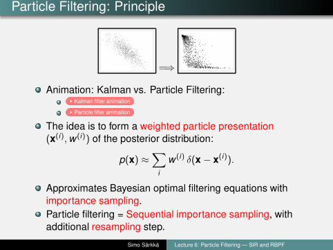
Animation: Kalman vs. Particle Filtering:Kalman filter animation
Particle filter animation
The idea is to form a weighted particle presentation
(x(i),w (i)) of the posterior distribution:
p(x) ≈∑
i
w (i) δ(x − x(i)).
Approximates Bayesian optimal filtering equations with
importance sampling.
Particle filtering = Sequential importance sampling, with
additional resampling step.
Simo Särkkä Lecture 6: Particle Filtering — SIR and RBPF
Monte Carlo Integration
−6 −4 −2 0 2 4 6−6
−4
−2
0
2
4
6
x−coordinate
y−co
ordi
nate
−6 −4 −2 0 2 4 6−6
−4
−2
0
2
4
6
x−coordinate
y−co
ordi
nate
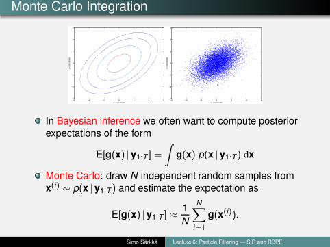
In Bayesian inference we often want to compute posterior
expectations of the form
E[g(x) |y1:T ] =
∫
g(x) p(x |y1:T ) dx
Monte Carlo: draw N independent random samples from
x(i) ∼ p(x |y1:T ) and estimate the expectation as
E[g(x) |y1:T ] ≈1
N
N∑
i=1
g(x(i)).
Simo Särkkä Lecture 6: Particle Filtering — SIR and RBPF
Importance Sampling: Basic Version [1/2]
−4 −3 −2 −1 0 1 2 3 40
0.05
0.1
0.15
0.2
0.25
0.3
0.35
0.4
x
Pro
babi
lity
Target distributionImportance Distribution
−3 −2 −1 0 1 2 30
0.2
0.4
0.6
0.8
1
1.2
1.4
x
Wei
ght
Weighted sample
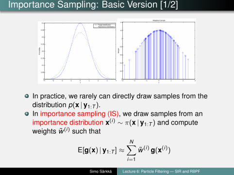
In practice, we rarely can directly draw samples from the
distribution p(x |y1:T ).
In importance sampling (IS), we draw samples from an
importance distribution x(i) ∼ π(x |y1:T ) and compute
weights w̃ (i) such that
E[g(x) |y1:T ] ≈
N∑
i=1
w̃ (i) g(x(i))
Simo Särkkä Lecture 6: Particle Filtering — SIR and RBPF
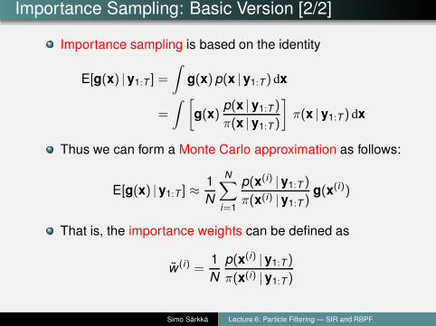
Importance Sampling: Basic Version [2/2]
Importance sampling is based on the identity
E[g(x) |y1:T ] =
∫
g(x)p(x |y1:T ) dx
=
∫ [
g(x)p(x |y1:T )
π(x |y1:T )
]
π(x |y1:T ) dx
Thus we can form a Monte Carlo approximation as follows:
E[g(x) |y1:T ] ≈1
N
N∑
i=1
p(x(i) |y1:T )
π(x(i) |y1:T )g(x(i))
That is, the importance weights can be defined as
w̃ (i) =1
N
p(x(i) |y1:T )
π(x(i) |y1:T )
Simo Särkkä Lecture 6: Particle Filtering — SIR and RBPF
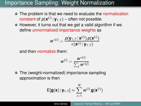
Importance Sampling: Weight Normalization
The problem is that we need to evaluate the normalization
constant of p(x(i) |y1:T ) – often not possible.
However, it turns out that we get a valid algorithm if we
define unnormalized importance weights as
w∗(i) =p(y1:T |x(i))p(x(i))
π(x(i) |y1:T )
and then normalize them:
w (i) =w∗(i)
∑
j w∗(j)
The (weight-normalized) importance sampling
approximation is then
E[g(x) |y1:T ] ≈
N∑
i=1
w (i) g(x(i))
Simo Särkkä Lecture 6: Particle Filtering — SIR and RBPF
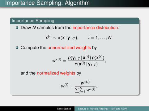
Importance Sampling: Algorithm
Importance Sampling
Draw N samples from the importance distribution:
x(i) ∼ π(x |y1:T ), i = 1, . . . ,N.
Compute the unnormalized weights by
w∗(i) =p(y1:T |x(i))p(x(i))
π(x(i) |y1:T ),
and the normalized weights by
w (i) =w∗(i)
∑Nj=1 w∗(j)
.
Simo Särkkä Lecture 6: Particle Filtering — SIR and RBPF
Importance Sampling: Properties
The approximation to the posterior expectation of g(x) is
then given as
E[g(x) |y1:T ] ≈
N∑
i=1
w (i) g(x(i)).
The posterior probability density approximation can then
be formally written as
p(x |y1:T ) ≈
N∑
i=1
w (i) δ(x − x(i)),
where δ(·) is the Dirac delta function.
The efficiency depends on the choice of the importance
distribution.
Simo Särkkä Lecture 6: Particle Filtering — SIR and RBPF
Sequential Importance Sampling: Idea
Sequential Importance Sampling (SIS) is concerned with
models
xk ∼ p(xk | xk−1)
yk ∼ p(yk | xk )
The SIS algorithm uses a weighted set of particles
{(w(i)k ,x
(i)k ) : i = 1, . . . ,N} such that
E[g(xk ) |y1:k ] ≈
N∑
i=1
w(i)k g(x
(i)k ).
Or equivalently
p(xk |y1:k) ≈
N∑
i=1
w(i)k δ(xk − x
(i)k ),
where δ(·) is the Dirac delta function.
Uses importance sampling sequentially.
Simo Särkkä Lecture 6: Particle Filtering — SIR and RBPF
Sequential Importance Sampling: Derivation [1/2]
Let’s consider the full posterior distribution of states x0:k
given the measurements y1:k .
We get the following recursion for the posterior distribution:
p(x0:k |y1:k) ∝ p(yk |x0:k ,y1:k−1)p(x0:k |y1:k−1)
= p(yk |xk )p(xk |x0:k−1,y1:k−1)p(x0:k−1 |y1:k−1)
= p(yk |xk )p(xk |xk−1)p(x0:k−1 |y1:k−1).
We could now construct an importance distribution
x(i)0:k ∼ π(x0:k |y1:k ) and compute the corresponding
(normalized) importance weights as
w(i)k ∝
p(yk |x(i)k )p(x
(i)k |x
(i)k−1)p(x
(i)0:k−1 |y1:k−1)
π(x(i)0:k |y1:k)
.
Simo Särkkä Lecture 6: Particle Filtering — SIR and RBPF
Sequential Importance Sampling: Derivation [2/2]
Let’s form the importance distribution recursively as
follows:
π(x0:k |y1:k) = π(xk |x0:k−1,y1:k )π(x0:k−1 |y1:k−1)
Expression for the importance weights can be written as
w(i)k ∝
p(yk |x(i)k )p(x
(i)k |x
(i)k−1)
π(x(i)k |x
(i)0:k−1,y1:k)
p(x(i)0:k−1 |y1:k−1)
π(x(i)0:k−1 |y1:k−1)
︸ ︷︷ ︸
∝w(i)k−1
Thus the weights satisfy the recursion
w(i)k ∝
p(yk |x(i)k )p(x
(i)k |x
(i)k−1)
π(x(i)k |x
(i)0:k−1,y1:k )
w(i)k−1
Simo Särkkä Lecture 6: Particle Filtering — SIR and RBPF
Sequential Importance Sampling: Algorithm
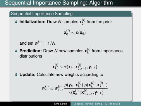
Sequential Importance Sampling
Initialization: Draw N samples x(i)0 from the prior
x(i)0 ∼ p(x0)
and set w(i)0 = 1/N.
Prediction: Draw N new samples x(i)k from importance
distributions
x(i)k ∼ π(xk |x
(i)0:k−1,y1:k)
Update: Calculate new weights according to
w(i)k ∝ w
(i)k−1
p(yk |x(i)k ) p(x
(i)k |x
(i)k−1)
π(x(i)k |x
(i)0:k−1,y1:k )
Simo Särkkä Lecture 6: Particle Filtering — SIR and RBPF
Sequential Importance Sampling: Degeneracy
The problem in SIS is that the algorithm is degenerate
It can be shown that the variance of the weights increases
at every step
It means that we will always converge to single non-zero
weight w (i) = 1 and the rest being zero – not very useful
algorithm.
Solution: resampling!
Simo Särkkä Lecture 6: Particle Filtering — SIR and RBPF
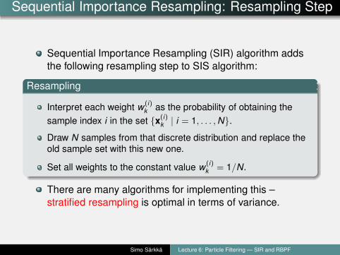
Sequential Importance Resampling: Resampling Step
Sequential Importance Resampling (SIR) algorithm adds
the following resampling step to SIS algorithm:
Resampling
Interpret each weight w(i)k as the probability of obtaining the
sample index i in the set {x(i)k | i = 1, . . . ,N}.
Draw N samples from that discrete distribution and replace theold sample set with this new one.
Set all weights to the constant value w(i)k = 1/N.
There are many algorithms for implementing this –
stratified resampling is optimal in terms of variance.
Simo Särkkä Lecture 6: Particle Filtering — SIR and RBPF
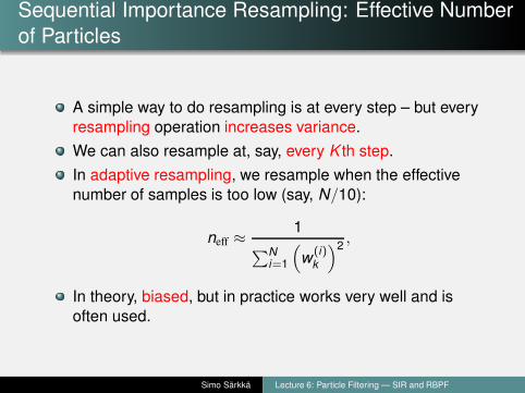
Sequential Importance Resampling: Effective Number
of Particles
A simple way to do resampling is at every step – but every
resampling operation increases variance.
We can also resample at, say, every K th step.
In adaptive resampling, we resample when the effective
number of samples is too low (say, N/10):
neff ≈1
∑Ni=1
(
w(i)k
)2,
In theory, biased, but in practice works very well and is
often used.
Simo Särkkä Lecture 6: Particle Filtering — SIR and RBPF
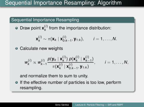
Sequential Importance Resampling: Algorithm
Sequential Importance Resampling
Draw point x(i)k from the importance distribution:
x(i)k ∼ π(xk | x
(i)0:k−1,y1:k), i = 1, . . . ,N.
Calculate new weights
w(i)k ∝ w
(i)k−1
p(yk | x(i)k ) p(x
(i)k | x
(i)k−1)
π(x(i)k | x
(i)0:k−1,y1:k )
, i = 1, . . . ,N,
and normalize them to sum to unity.
If the effective number of particles is too low, perform
resampling.
Simo Särkkä Lecture 6: Particle Filtering — SIR and RBPF
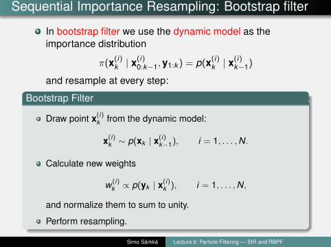
Sequential Importance Resampling: Bootstrap filter
In bootstrap filter we use the dynamic model as the
importance distribution
π(x(i)k | x
(i)0:k−1,y1:k ) = p(x
(i)k | x
(i)k−1)
and resample at every step:
Bootstrap Filter
Draw point x(i)k from the dynamic model:
x(i)k ∼ p(xk | x
(i)k−1), i = 1, . . . ,N.
Calculate new weights
w(i)k ∝ p(yk | x
(i)k ), i = 1, . . . ,N,
and normalize them to sum to unity.
Perform resampling.
Simo Särkkä Lecture 6: Particle Filtering — SIR and RBPF
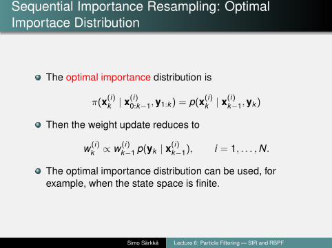
Sequential Importance Resampling: Optimal
Importace Distribution
The optimal importance distribution is
π(x(i)k | x
(i)0:k−1,y1:k) = p(x
(i)k | x
(i)k−1,yk )
Then the weight update reduces to
w(i)k ∝ w
(i)k−1 p(yk | x
(i)k−1), i = 1, . . . ,N.
The optimal importance distribution can be used, for
example, when the state space is finite.
Simo Särkkä Lecture 6: Particle Filtering — SIR and RBPF
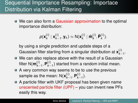
Sequential Importance Resampling: Importace
Distribution via Kalman Filtering
We can also form a Gaussian approximation to the optimal
importance distribution:
p(x(i)k | x
(i)k−1,yk ) ≈ N(x
(i)k | m̃
(i)k , P̃
(i)k ).
by using a single prediction and update steps of a
Gaussian filter starting from a singular distribution at x(i)k−1.
We can also replace above with the result of a Gaussian
filter N(m(i)k−1,P
(i)k−1) started from a random initial mean.
A very common way seems to be to use the previous
sample as the mean: N(x(i)k−1,P
(i)k−1).
A particle filter with UKF proposal has been given name
unscented particle filter (UPF) – you can invent new PFs
easily this way.
Simo Särkkä Lecture 6: Particle Filtering — SIR and RBPF
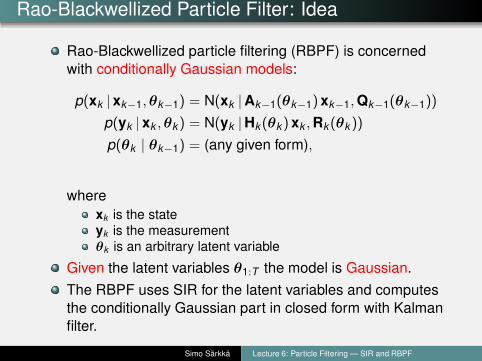
Rao-Blackwellized Particle Filter: Idea
Rao-Blackwellized particle filtering (RBPF) is concerned
with conditionally Gaussian models:
p(xk |xk−1,θk−1) = N(xk |Ak−1(θk−1)xk−1,Qk−1(θk−1))
p(yk |xk ,θk ) = N(yk |Hk (θk )xk ,Rk (θk ))
p(θk | θk−1) = (any given form),
where
xk is the state
yk is the measurement
θk is an arbitrary latent variable
Given the latent variables θ1:T the model is Gaussian.
The RBPF uses SIR for the latent variables and computes
the conditionally Gaussian part in closed form with Kalman
filter.
Simo Särkkä Lecture 6: Particle Filtering — SIR and RBPF
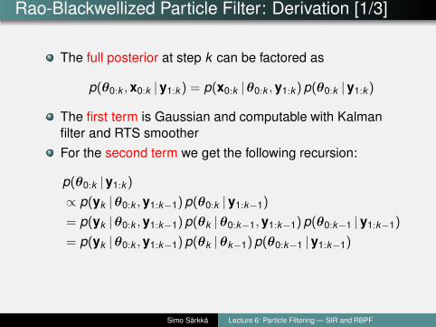
Rao-Blackwellized Particle Filter: Derivation [1/3]
The full posterior at step k can be factored as
p(θ0:k ,x0:k |y1:k ) = p(x0:k |θ0:k ,y1:k)p(θ0:k |y1:k )
The first term is Gaussian and computable with Kalman
filter and RTS smoother
For the second term we get the following recursion:
p(θ0:k |y1:k )
∝ p(yk |θ0:k ,y1:k−1)p(θ0:k |y1:k−1)
= p(yk |θ0:k ,y1:k−1)p(θk |θ0:k−1,y1:k−1)p(θ0:k−1 |y1:k−1)
= p(yk |θ0:k ,y1:k−1)p(θk |θk−1)p(θ0:k−1 |y1:k−1)
Simo Särkkä Lecture 6: Particle Filtering — SIR and RBPF
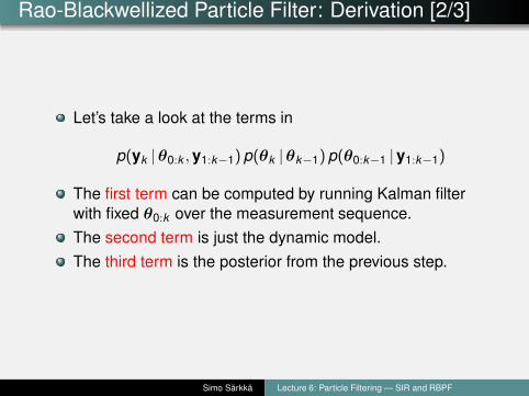
Rao-Blackwellized Particle Filter: Derivation [2/3]
Let’s take a look at the terms in
p(yk |θ0:k ,y1:k−1)p(θk |θk−1)p(θ0:k−1 |y1:k−1)
The first term can be computed by running Kalman filter
with fixed θ0:k over the measurement sequence.
The second term is just the dynamic model.
The third term is the posterior from the previous step.
Simo Särkkä Lecture 6: Particle Filtering — SIR and RBPF
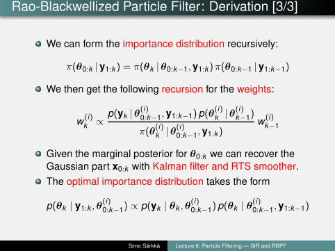
Rao-Blackwellized Particle Filter: Derivation [3/3]
We can form the importance distribution recursively:
π(θ0:k |y1:k ) = π(θk |θ0:k−1,y1:k)π(θ0:k−1 |y1:k−1)
We then get the following recursion for the weights:
w(i)k ∝
p(yk |θ(i)0:k−1,y1:k−1)p(θ
(i)k |θ
(i)k−1)
π(θ(i)k |θ
(i)0:k−1,y1:k )
w(i)k−1
Given the marginal posterior for θ0:k we can recover the
Gaussian part x0:k with Kalman filter and RTS smoother.
The optimal importance distribution takes the form
p(θk | y1:k ,θ(i)0:k−1) ∝ p(yk | θk ,θ
(i)0:k−1)p(θk | θ
(i)0:k−1,y1:k−1)
Simo Särkkä Lecture 6: Particle Filtering — SIR and RBPF
Rao-Blackwellized Particle Filter: Algorithm [1/3]
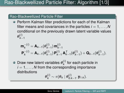
Rao-Blackwellized Particle Filter
Perform Kalman filter predictions for each of the Kalman
filter means and covariances in the particles i = 1, . . . ,Nconditional on the previously drawn latent variable values
θ(i)k−1
m−(i)k = Ak−1(θ
(i)k−1)m
(i)k−1
P−(i)k = Ak−1(θ
(i)k−1)P
(i)k−1 AT
k−1(θ(i)k−1) + Qk−1(θ
(i)k−1).
Draw new latent variables θ(i)k for each particle in
i = 1, . . . ,N from the corresponding importance
distributions
θ(i)k ∼ π(θk | θ
(i)0:k−1,y1:k ).
Simo Särkkä Lecture 6: Particle Filtering — SIR and RBPF
Rao-Blackwellized Particle Filter: Algorithm [2/3]
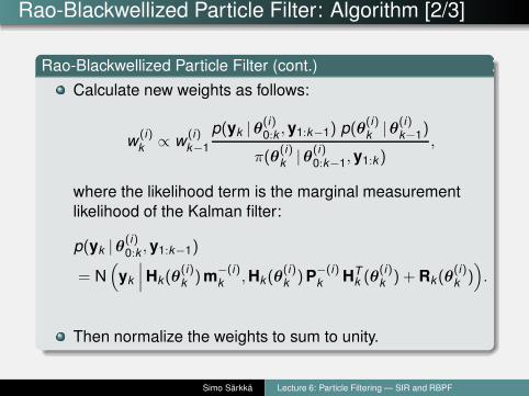
Rao-Blackwellized Particle Filter (cont.)
Calculate new weights as follows:
w(i)k ∝ w
(i)k−1
p(yk |θ(i)0:k ,y1:k−1) p(θ
(i)k |θ
(i)k−1)
π(θ(i)k |θ
(i)0:k−1,y1:k)
,
where the likelihood term is the marginal measurement
likelihood of the Kalman filter:
p(yk |θ(i)0:k ,y1:k−1)
= N(
yk
∣∣∣Hk(θ
(i)k )m
−(i)k ,Hk (θ
(i)k )P
−(i)k HT
k (θ(i)k ) + Rk (θ
(i)k )
)
.
Then normalize the weights to sum to unity.
Simo Särkkä Lecture 6: Particle Filtering — SIR and RBPF
Rao-Blackwellized Particle Filter: Algorithm [3/3]
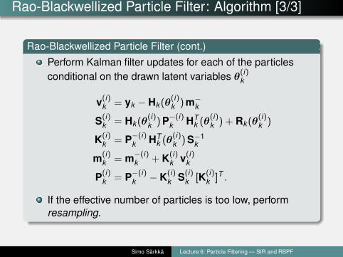
Rao-Blackwellized Particle Filter (cont.)
Perform Kalman filter updates for each of the particles
conditional on the drawn latent variables θ(i)k
v(i)k = yk − Hk (θ
(i)k )m−
k
S(i)k = Hk(θ
(i)k )P
−(i)k HT
k (θ(i)k ) + Rk(θ
(i)k )
K(i)k = P
−(i)k HT
k (θ(i)k )S−1
k
m(i)k = m
−(i)k + K
(i)k v
(i)k
P(i)k = P
−(i)k − K
(i)k S
(i)k [K
(i)k ]T .
If the effective number of particles is too low, perform
resampling.
Simo Särkkä Lecture 6: Particle Filtering — SIR and RBPF
Rao-Blackwellized Particle Filter: Properties
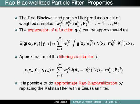
The Rao-Blackwellized particle filter produces a set of
weighted samples {w(i)k ,θ
(i)k ,m
(i)k ,P
(i)k : i = 1, . . . ,N}
The expectation of a function g(·) can be approximated as
E[g(xk ,θk ) |y1:k ] ≈N∑
i=1
w(i)k
∫
g(xk ,θ(i)k ) N(xk |m
(i)k ,P
(i)k ) dxk .
Approximation of the filtering distribution is
p(xk ,θk |y1:k ) ≈
N∑
i=1
w(i)k δ(θk − θ
(i)k ) N(xk |m
(i)k ,P
(i)k ).
It is possible to do approximate Rao-Blackwellization by
replacing the Kalman filter with a Gaussian filter.
Simo Särkkä Lecture 6: Particle Filtering — SIR and RBPF
Rao-Blackwellization of Static Parameters
Rao-Blackwellization can sometimes be used in models of
the form
xk ∼ p(xk |xk−1,θ)
yk ∼ p(yk |xk ,θ)
θ ∼ p(θ),
where vector θ contains the unknown static parameters.
Possible if the posterior distribution of parameters θ
depends only on some sufficient statistics Tk :
Tk = Tk(x1:k ,y1:k)
We also need to have a recursion rule for the sufficient
statistics.
Can be extended to time-varying parameters.
Simo Särkkä Lecture 6: Particle Filtering — SIR and RBPF
Particle Filter: Advantages
No restrictions in model – can be applied to non-Gaussian
models, hierarchical models etc.
Global approximation.
Approaches the exact solution, when the number of
samples goes to infinity.
In its basic form, very easy to implement.
Superset of other filtering methods – Kalman filter is a
Rao-Blackwellized particle filter with one particle.
Simo Särkkä Lecture 6: Particle Filtering — SIR and RBPF
Particle Filter: Disadvantages
Computational requirements much higher than of the
Kalman filters.
Problems with nearly noise-free models, especially with
accurate dynamic models.
Good importance distributions and efficient
Rao-Blackwellized filters quite tricky to implement.
Very hard to find programming errors (i.e., to debug).
Simo Särkkä Lecture 6: Particle Filtering — SIR and RBPF
Summary
Particle filters use weighted set of samples (particles) for
approximating the filtering distributions.
Sequential importance resampling (SIR) is the general
framework and bootstrap filter is a simple special case of it.
EKF, UKF and other Gaussian filters can be used for
forming good importance distributions.
In Rao-Blackwellized particle filters a part of the state is
sampled and part is integrated in closed form with Kalman
filter.
Simo Särkkä Lecture 6: Particle Filtering — SIR and RBPF
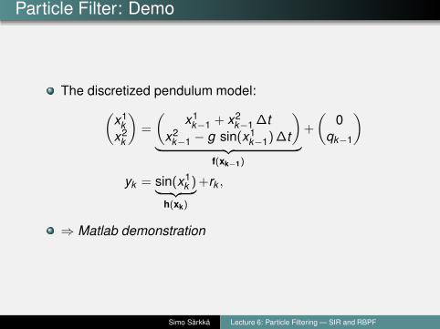
Particle Filter: Demo
The discretized pendulum model:
(x1
k
x2k
)
=
(x1
k−1 + x2k−1 ∆t
x2k−1 − g sin(x1
k−1)∆t
)
︸ ︷︷ ︸
f(xk−1)
+
(0
qk−1
)
yk = sin(x1k )
︸ ︷︷ ︸
h(xk)
+rk ,
⇒ Matlab demonstration
Simo Särkkä Lecture 6: Particle Filtering — SIR and RBPF


![H2E: A Privacy Provisioning Framework for Collaborative Filtering … · 2019-09-10 · collaborative filtering, content-based filtering, and hybrid filtering [3]. Content-based filtering,](https://img.pdfslide.us/doc/110x75/5f2811153d39b70bb31af3b8/h2e-a-privacy-provisioning-framework-for-collaborative-filtering-2019-09-10-collaborative.jpg)