PARTIALLY BLIND DEBLURRING OF BARCODE FROM …jxin/out_focus_blur_cam13-4… · · 2013-07-30PARTIALLY BLIND DEBLURRING OF BARCODE FROM OUT-OF-FOCUS BLUR YIFEI LOU, ERNIE ESSER,

PARTIALLY BLIND DEBLURRING OF BARCODE FROM OUT-OF-FOCUS BLUR

YIFEI LOU, ERNIE ESSER, HONGKAI ZHAO AND JACK XIN∗

Abstract. This paper addresses the nonstationary out-of-focus (OOF) blur removal in the application of barcodereconstruction. We propose a partially blind deblurring method when partial knowledge of the clean barcode is available.In particular, we consider an image formation model based on geometrical optics, which involves the point-spread function(PSF) for the OOF blur. With the known information, we can estimate a low-dimensional representation of the PSFusing the Levenberg-Marquardt algorithm. Once the PSF is obtained, the image deblurring is followed by quadraticprogramming. We find [0,1] box constraint is often good enough to enforce binary signal. Experiments on the real datademonstrate that the forward model is physically realistic and our partially blind deblurring method can yield goodreconstructions.

Key words. barcode, out-of-focus blur, geometrical optics, Levenberg-Marquardt algorithm, quadratic program-ming, box constraint

AMS subject classifications.

90C90, 65K10, 49N45, 49M20, 78A05

1. Introduction . Image restoration from out-of-focus (OOF) blur is a very difficult problem,as one has to infer both the original image and the point-spread function (PSF) from the data. Mostconventional methods model the OOF blur as a uniform disk [29, 25] and hence the PSF estimationreduces to estimating the radius of the blur disk [27]. However, in the real scenario, the OOF bluris not uniform, but dependent on the geometry of the object. The nonstationary nature makes manyblind deconvolution methods [7, 2, 24] unapplicable for the OOF blur removal. One way to managespatially variant blur is to segment the data into regions, on each of which blur is approximatelyinvariant. This idea has been explored in [28, 21, 8, 5]. However, deblurring results suffer from ringingartifacts due to the inconsistency of boundaries between different regions. A related line of research inmodeling the OOF blur is the shape from defocus [14, 16]. Although the main focus is to reconstructthe 3D geometry of a scene from a set of defocused images, image deblurring can be a byproduct.However, this type of approach often requires a well-calibrated camera and multiple images as input,which limits their usage in image deblurring from the OOF blur.

We attempt to solve this OOF deblurring problem in the application of barcode reconstruction.Standard commercial techniques are based on classic edge detection [22, 23]. Since edges are importantfor barcode decoding, one searches for local extrema of the derivative of the signal, which hopefullycorrespond to edges. However, this approach has two main drawbacks. First of all, the derivative ishighly sensitive to small changes in the data, such as noise. In addition, some edges in the originalbarcode may not have corresponding extrema in the corrupted data if the blur is relatively large. Analternative direction of barcode decoding is to view it as a deblurring problem. Most of works assumethat the PSF is a shift-invariant kernel and then blind or nonblind deconvolution is formulated toreconstruct the barcode. For example, variational models are discussed in [12, 9]. Recently, Iwen et.al. [20] develop a sparse representation of the barcode by exploiting the barcode symbology. Thesemethods are not exactly blind, but can deal with small amount of blurring and noise.

We propose a partially blind method to recover binary barcode. It is based on an image formationmodel for out-of-focus blur [15]. We first estimate a low-dimensional approximation to the PSF byusing some parts of clean barcode that are known by construction. This low-dim representation onlyinvolves a few parameters, which can be iteratively computed via the Levenberg-Marquardt (LM)algorithm. The rest of the PSF is obtained by polynomial interpolations. Next, image deblurring isperformed by solving the least-square (LS) solution with additional constraint that the variables arebounded by 0 and 1, i.e. [0, 1] box constraint. We further take the minimum bar width into account,which corresponds to a stretching matrix or an up-sampling operator. Having this matrix in the LS

∗ All authors are from Department of Mathematics, UC Irvine, Irvine, CA 92697. Emails: [email protected],[email protected], [email protected], [email protected].

1

2 Y. Lou, E. Esser, H. Zhao and J. Xin

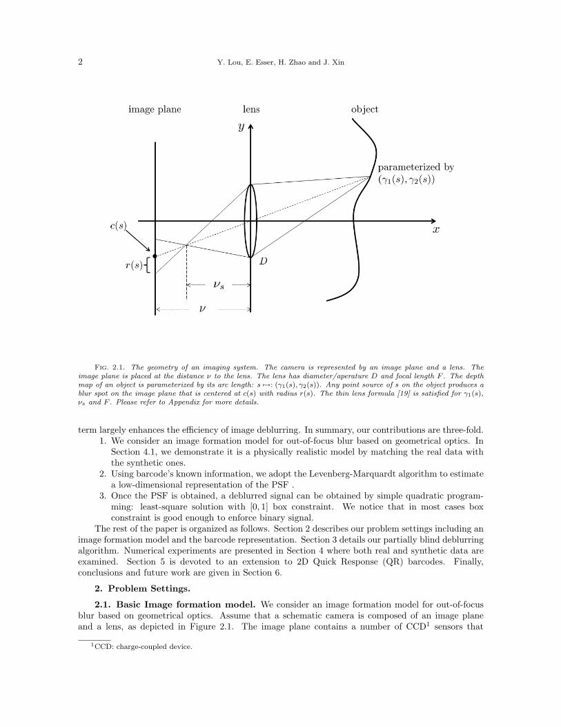
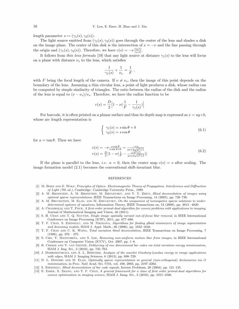
Fig. 2.1. The geometry of an imaging system. The camera is represented by an image plane and a lens. Theimage plane is placed at the distance ν to the lens. The lens has diameter/aperature D and focal length F . The depthmap of an object is parameterized by its arc length: s 7→: (γ1(s), γ2(s)). Any point source of s on the object produces ablur spot on the image plane that is centered at c(s) with radius r(s). The thin lens formula [19] is satisfied for γ1(s),νs and F . Please refer to Appendix for more details.

term largely enhances the efficiency of image deblurring. In summary, our contributions are three-fold.1. We consider an image formation model for out-of-focus blur based on geometrical optics. In

Section 4.1, we demonstrate it is a physically realistic model by matching the real data withthe synthetic ones.

2. Using barcode’s known information, we adopt the Levenberg-Marquardt algorithm to estimatea low-dimensional representation of the PSF .

3. Once the PSF is obtained, a deblurred signal can be obtained by simple quadratic program-ming: least-square solution with [0, 1] box constraint. We notice that in most cases boxconstraint is good enough to enforce binary signal.

The rest of the paper is organized as follows. Section 2 describes our problem settings including animage formation model and the barcode representation. Section 3 details our partially blind deblurringalgorithm. Numerical experiments are presented in Section 4 where both real and synthetic data areexamined. Section 5 is devoted to an extension to 2D Quick Response (QR) barcodes. Finally,conclusions and future work are given in Section 6.

2. Problem Settings.

2.1. Basic Image formation model. We consider an image formation model for out-of-focusblur based on geometrical optics. Assume that a schematic camera is composed of an image planeand a lens, as depicted in Figure 2.1. The image plane contains a number of CCD1 sensors that

1CCD: charge-coupled device.

Partially blind deblurring of barcode from out-of-focus blur 3

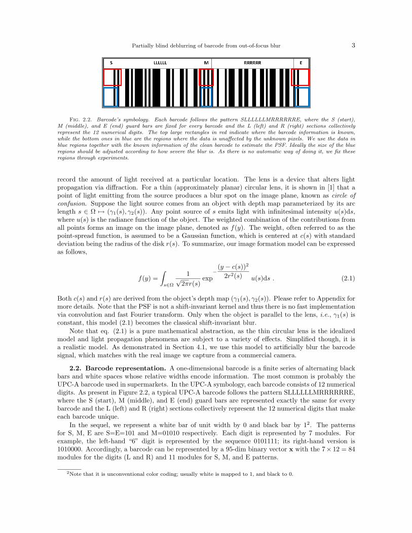
Fig. 2.2. Barcode’s symbology. Each barcode follows the pattern SLLLLLLMRRRRRRE, where the S (start),M (middle), and E (end) guard bars are fixed for every barcode and the L (left) and R (right) sections collectivelyrepresent the 12 numerical digits. The top large rectangles in red indicate where the barcode information is known,while the bottom ones in blue are the regions where the data is unaffected by the unknown pixels. We use the data inblue regions together with the known information of the clean barcode to estimate the PSF. Ideally the size of the blueregions should be adjusted according to how severe the blur is. As there is no automatic way of doing it, we fix theseregions through experiments.

record the amount of light received at a particular location. The lens is a device that alters lightpropagation via diffraction. For a thin (approximately planar) circular lens, it is shown in [1] that apoint of light emitting from the source produces a blur spot on the image plane, known as circle ofconfusion. Suppose the light source comes from an object with depth map parameterized by its arclength s ∈ Ω 7→ (γ1(s), γ2(s)). Any point source of s emits light with infinitesimal intensity u(s)ds,where u(s) is the radiance function of the object. The weighted combination of the contributions fromall points forms an image on the image plane, denoted as f(y). The weight, often referred to as thepoint-spread function, is assumed to be a Gaussian function, which is centered at c(s) with standarddeviation being the radius of the disk r(s). To summarize, our image formation model can be expressedas follows,

f(y) =∫

s∈Ω

1√2πr(s)

exp−

(y − c(s))2

2r2(s) u(s)ds . (2.1)

Both c(s) and r(s) are derived from the object’s depth map (γ1(s), γ2(s)). Please refer to Appendix formore details. Note that the PSF is not a shift-invariant kernel and thus there is no fast implementationvia convolution and fast Fourier transform. Only when the object is parallel to the lens, i.e., γ1(s) isconstant, this model (2.1) becomes the classical shift-invariant blur.

Note that eq. (2.1) is a pure mathematical abstraction, as the thin circular lens is the idealizedmodel and light propagation phenomena are subject to a variety of effects. Simplified though, it isa realistic model. As demonstrated in Section 4.1, we use this model to artificially blur the barcodesignal, which matches with the real image we capture from a commercial camera.

2.2. Barcode representation. A one-dimensional barcode is a finite series of alternating blackbars and white spaces whose relative widths encode information. The most common is probably theUPC-A barcode used in supermarkets. In the UPC-A symbology, each barcode consists of 12 numericaldigits. As present in Figure 2.2, a typical UPC-A barcode follows the pattern SLLLLLLMRRRRRRE,where the S (start), M (middle), and E (end) guard bars are represented exactly the same for everybarcode and the L (left) and R (right) sections collectively represent the 12 numerical digits that makeeach barcode unique.

In the sequel, we represent a white bar of unit width by 0 and black bar by 12. The patternsfor S, M, E are S=E=101 and M=01010 respectively. Each digit is represented by 7 modules. Forexample, the left-hand “6” digit is represented by the sequence 0101111; its right-hand version is1010000. Accordingly, a barcode can be represented by a 95-dim binary vector x with the 7× 12 = 84modules for the digits (L and R) and 11 modules for S, M, and E patterns.

2Note that it is unconventional color coding; usually white is mapped to 1, and black to 0.


Given the blurred data f in (2.1), we exploit the known information of a barcode to estimate thePSF. For example, the patterns on the S, M, E regions are fixed for any barcode. In order to betterutilize the information on S and E regions, we elongate the binary vector x by zero padding on bothsides. This is reasonable, as the barcode is always surrounded by the white areas. More importantly,it contains useful information to understand how the boundary gets blurred. We further notice thatthe first and the last elements for each digit, no matter whether it appears in L or in R, are always thesame. We will use these regions, as indicated in red rectangles in Figure 2.2, where barcode informationis known to estimate the PSF.

3. Algorithm. We propose a “partially” blind restoration method in the sense that we exploitthe known barcode information to estimate the PSF. Then image deblurring is performed using theestimated PSF with additional constraint that the signal is binary.

3.1. Estimating the PSF. We compute the PSF based on obtained data and the known infor-mation of the barcode. For the out-of-focus blur, the PSF is characterized by the center and the blurradius of each point source, c(s) and r(s). We consider a low-dimensional representation by polynomialinterpolation . In particular, we approximate c(s) using 6 data points (two in each known region: S, Mand E), denoted as sj for j = 1, · · · , 6. Given values of c(s) at these 6 points, we can define a matrixP with each row being Pj = [s3

j s2j sj 1]. Denote c(s) as a third-order polynomial to approximate c(s):

c(s) = c3s3 + c2s

2 + c1s + c0 . (3.1)

The coefficients of c(s) can be calculated by a least-square fitting, i.e.,c3

c2

c1

c0

= (PT P )−1PT

c(s1)...

c(s6)

. (3.2)

Similarly we can obtain the polynomial r(s) to approximate r(s). The polynomial approximation isreasonable, considering that the depth map is continuous and so are c(s) and r(s). With polynomialinterpolations, the PSF is now dependent on 12 parameters θ = [c(sj), r(sj)]j=1,··· ,6, which is a largedimension reduction.

In order to estimate θ, we modify the image formation model (2.1) so that it explicitly dependson θ = θkk=1,··· ,12 and the known information of the barcode. Denote R as the region where thebarcode information is known. The discrete version of (2.1) is

f(y;θ) =∑

s∈R

1√2πr(s)

exp−

(y − c(s))2

2r2(s) u(s),

for c(s), r(s) being interpolated from θ.

(3.3)

We further restrict the domain of the data points by considering y ∈ B where the data is unaffected bythe unknown barcode. Notice that ideally we should adjust the data region B according to how severethe blur is. But as there is no automatic way of doing it, we fix the size of B through experiments. InFigure 2.2, the red triangles indicate the known barcode regions R, while the blue ones are the regionsB for the data points we use to estimate the PSF.

Given the known barcode signal x ∈ R and the data points y ∈ B, we adopt the Levenberg−Marquardt(LM) scheme to find θ that minimizes

S(θ) =∑y∈B

‖f(y)− f(y;θ)‖2. (3.4)

Since S(θ) is nonlinear and implicit with respect to θ, the Jacobian is computed numerically foreach component of θ,

Jk =1ε

(f(y;θ + ε1k)− f(y;θ)

), (3.5)


where 1k is an indicator vector with 1 at the index k. At every iteration, the increment δ is solvedfrom the linear system,

(JT J + λI)δ = JT [f(y)− f(y;θ)] . (3.6)

The parameter λ > 0 is adjusted at each iteration. If reduction of S is sufficient, a smaller value isused; whereas if an iteration gives insufficient reduction in the residual, we should increase its value.Once the values θ are obtained, we can compute c(s) and r(s) as approximations to c(s) and r(s) andaccordingly the PSF can be calculated via eq. (2.1).

Note that a fast alternative is to use a piece-wise convolution approximation to the full blurringmodel. However, experiments indicate that it is more prone to getting stuck in local minima, partlybecause fewer equations are used in order to avoid boundary artifacts.

3.2. Image deblurring. The discrete imaging model (2.1) can be expressed as matrix-vectormultiplication f = Hu. The blurring matrix H is estimated via the LM algorithm, as detailed in theprevious section.

We take into account the minimum bar width to reduce the computational cost. Suppose thebarcode signal x = [x1, · · · , xn] is of length n after zero padding. Consider the characteristic function

χ(t) =

1 for 0 6 t 6 1,0 else.

Then the barcode function can be further represented as

u(s) =n∑

j=1

xjχ(s

w− j) (3.7)

where w is the minimum bar width. In the discrete version, this is equivalent to u = Sx with S beinga stretch matrix. It can be defined in terms of the Kronecker product, i.e., S = In⊗1w, where In is anidentity matrix of size n and 1w is a column vector of length w with element 1. It is huge dimensionreduction to solve x instead of u.

Let A = HS. We formulate the image deblurring problem as a least-square fitting with binaryconstraint,

min ‖Ax− f‖2 s.t. x ∈ 0, 1 (3.8)

This is a non-convex problem due to the binary constraint. There are a couple of natural strategiesfor solving the original problem (3.8). One is to relax the binary constraint by box constraint (BX),

min ‖Ax− f‖2 s.t. 0 6 x 6 1 (3.9)

This is a quadratic programming problem, which is well-studied and can be solved by many opti-mization schemes. We adopt a modified primal dual hybrid gradient (PDHG) method [30] to solve it.The PDHG method [30] and its variants [4, 13, 18] can be used to solve general convex optimizationproblems of the form

minx

J(Ax) + H(x)

where J and H are closed proper convex functions. They find a minimizer x∗ by solving for a saddlepoint (x∗,y∗) of

L(x,y) = H(x) + 〈y, Ax〉 − J∗(y) .

A common variant of PDHG does this by iterating

yk+1 = arg miny

J∗(y)− 〈Axk,y〉+12δ‖y − yk‖2

xk+1 = arg minx

H(x) + 〈AT (2yk+1 − yk),x〉+12α

‖x− xk‖2 ,


where δ and α are positive parameters satisfying αδ < 1‖AT A‖ and J∗ denotes the Legendre transform or

convex conjugate of J . This method is especially useful when the J and H minimization subproblemscan be efficiently solved. Moreover, it is not necessary to explicitly construct the matrix A since themethod only requires that we be able to multiply by A and AT . For Problem (3.9), we let J(Ax) =

12‖Ax−f‖2 and H(x) = g[0,1](x), where g is an indicator function defined by g(x) =

0 if x ∈ [0, 1]∞ otherwise.

Since J∗(y) = 12‖y‖

2 + 〈f,y〉, the explicit iterations can be written in closed form as

yk+1 = (δAxk − δf + yk)/(1 + δ) (3.10)xk+1 = Π[0,1]

(xk − αAT (2yk+1 − yk)

)(3.11)

where Π[0,1] denotes the orthogonal projection onto [0, 1]. For this application, the method is closelyrelated to simple gradient projection, i.e. equivalent if δ = 1. There are accelerated variants to improvethe rate of convergence.

Another way is to enforce the binary constraint by using the double well (DW) potential [12]

x = arg min1εW (x) + ε‖Dx‖2 +

γ

2‖Ax− f‖2 (3.12)

where W (x) = x2(1 − x)2 and ε, γ are two positive parameters. Including the derivative term ‖Dx‖helps to suppress the spatial oscillations. Both DW without ‖Dx‖ and the box constraint (3.9) sufferfrom this artifact. We apply gradient descent to obtain the optimal solution:

xt = −1εW ′(x) +4x− γAT (Ax− f) . (3.13)

4. Numerical Experiments. We validate the image formation model (2.1) by matching the realdata with the synthetic ones. Deblurring results are present for both real data and synthetic ones. Wealso examine the performance of some components of our algorithm using synthetic data. Our Matlabsource codes are available for download at the project webpage: https://sites.google.com/site/louyifei/research/barcode.

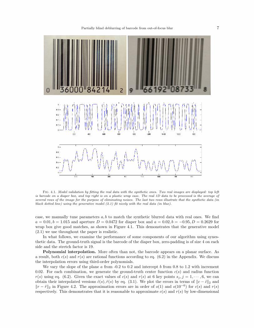
4.1. Model validation. We demonstrate the image formation model (2.1) is realistic by match-ing real signals with synthesized data. We take real images of barcodes. The top left plot in Figure 4.1is an image of Huggies diaper barcode printed on a box taken by Iphone5 and the more blurred oneon the right is of Kirkland’s plastic wrap barcode taken by Canon SLR Rebel XTi camera. Each rowof the image (except for the lower part with numbers) can be regarded as 1D corrupted barcode. Thereal data to be processed, denoted as f , is the average of a number of rows for the purpose of elimi-nating noises. We manually adjust the intensity value so that the synthetic data fit better with thereal ones. An automatic way of intensity fitting is addressed in Section 4.2. The intensity transformsare 1.2 − 1.6f and 1 − 1.38f for diaper box and wrap case respectively. The negative sign is due tobarcode’s unconventional color coding that maps white to 0 and black to 1.

To compare the real data with the synthetic ones, we first estimate the bar width from the dataf . We detect its local minima, each ideally corresponding to the center of black bar. Using the factthat the barcode is a 95-dim binary vector, we set the bar width to be the number of pixels betweenthe first and the last minimum locations divided by 94. The division by 94 instead of 95 is becausethat half bars on two ends are not counted in the range of two minima. The bar width of the diaperbox is calculated as 18.6, and we round it off to 19. The bar width for the wrap case is 8.

We synthesize blurred data from the model (2.1) in the following way. We generate a ground-truthbarcode using 12-number digits present in the image. For diaper box, we pad its 95-dim vector withsix ‘0’s on two sides and stretch it by a factor of 19. Similarly for the wrap case except that the stretchfactor is 8. We fix the camera parameters to be: focal length F = 12e − 3, distance between imageplane and the lens ν = 0.01285. Since the depth map is a linear function for both diaper box and wrap


Fig. 4.1. Model validation by fitting the real data with the synthetic ones. Two real images are displayed: top leftis barcode on a diaper box, and top right is on a plastic wrap case. The real 1D data to be processed is the average ofseveral rows of the image for the purpose of eliminating noises. The last two rows illustrate that the synthetic data (inblack dotted line) using the generative model (2.1) fit nicely with the real data (in blue).

case, we manually tune parameters a, b to match the synthetic blurred data with real ones. We finda = 0.01, b = 1.015 and aperture D = 0.0472 for diaper box and a = 0.02, b = −0.95, D = 0.2629 forwrap box give good matches, as shown in Figure 4.1. This demonstrates that the generative model(2.1) we use throughout the paper is realistic.

In what follows, we examine the performance of some components of our algorithm using synes-thetic data. The ground-truth signal is the barcode of the diaper box, zero-padding is of size 4 on eachside and the stretch factor is 19.

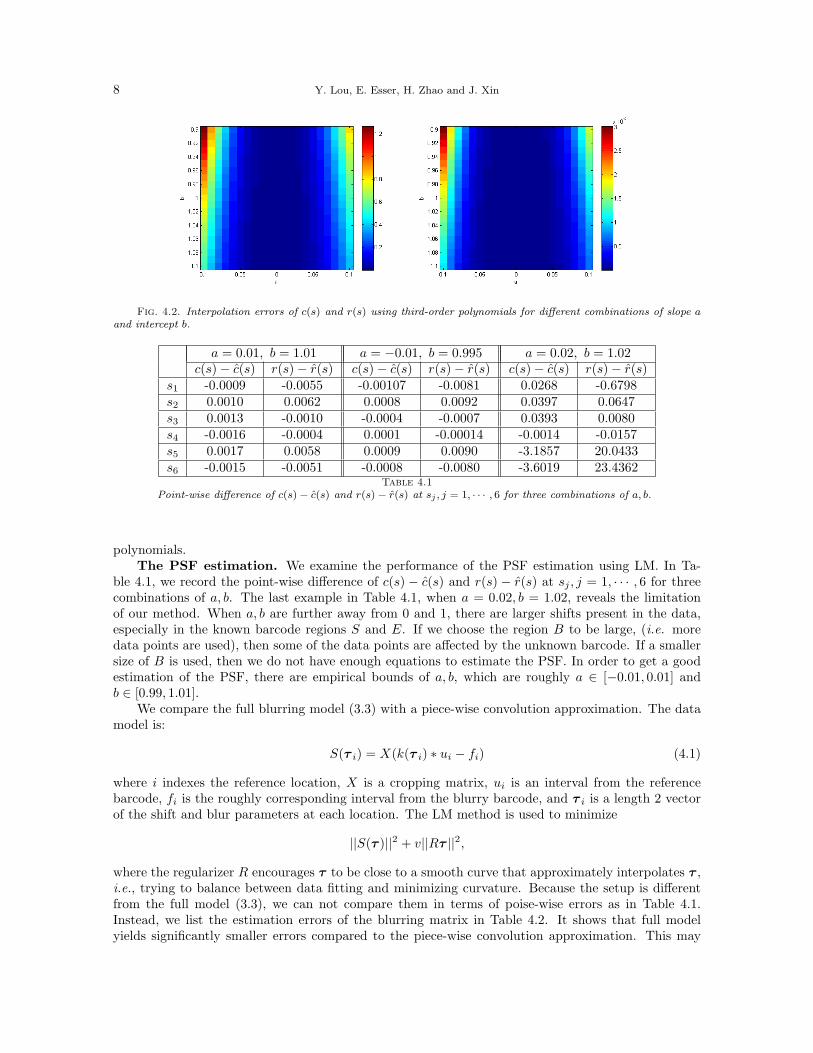
Polynomial interpolation. More often than not, the barcode appears on a planar surface. Asa result, both c(s) and r(s) are rational functions according to eq. (6.2) in the Appendix. We discussthe interpolation errors using third-order polynomials.

We vary the slope of the plane a from -0.2 to 0.2 and intercept b from 0.8 to 1.2 with increment0.02. For each combination, we generate the ground-truth center function c(s) and radius functionr(s) using eq. (6.2). Given the exact values of c(s) and r(s) at 6 key points sj , j = 1, · · · , 6, we canobtain their interpolated versions c(s), r(s) by eq. (3.1). We plot the errors in terms of ‖c − c‖2 and‖r − r‖2 in Figure 4.2. The approximation errors are in order of o(1) and o(10−6) for c(s) and r(s)respectively. This demonstrates that it is reasonable to approximate c(s) and r(s) by low-dimensional


Fig. 4.2. Interpolation errors of c(s) and r(s) using third-order polynomials for different combinations of slope aand intercept b.

a = 0.01, b = 1.01 a = −0.01, b = 0.995 a = 0.02, b = 1.02c(s)− c(s) r(s)− r(s) c(s)− c(s) r(s)− r(s) c(s)− c(s) r(s)− r(s)

s1 -0.0009 -0.0055 -0.00107 -0.0081 0.0268 -0.6798s2 0.0010 0.0062 0.0008 0.0092 0.0397 0.0647s3 0.0013 -0.0010 -0.0004 -0.0007 0.0393 0.0080s4 -0.0016 -0.0004 0.0001 -0.00014 -0.0014 -0.0157s5 0.0017 0.0058 0.0009 0.0090 -3.1857 20.0433s6 -0.0015 -0.0051 -0.0008 -0.0080 -3.6019 23.4362

Table 4.1Point-wise difference of c(s)− c(s) and r(s)− r(s) at sj , j = 1, · · · , 6 for three combinations of a, b.

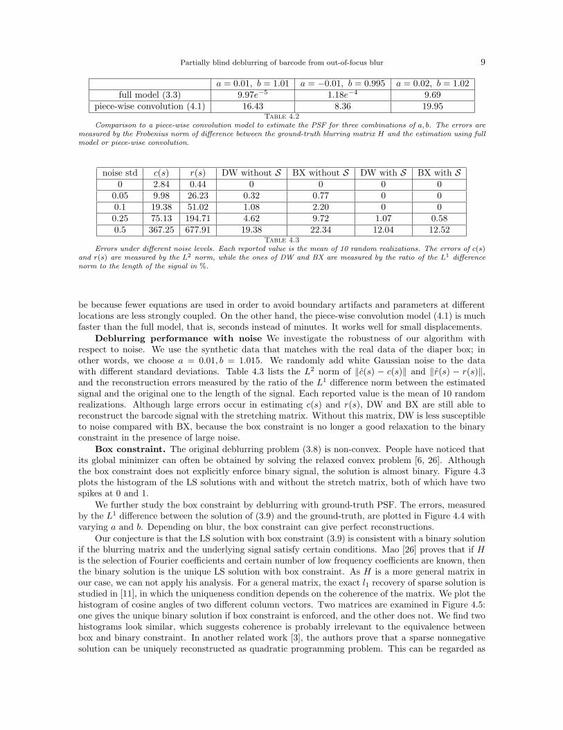
polynomials.The PSF estimation. We examine the performance of the PSF estimation using LM. In Ta-

ble 4.1, we record the point-wise difference of c(s) − c(s) and r(s) − r(s) at sj , j = 1, · · · , 6 for threecombinations of a, b. The last example in Table 4.1, when a = 0.02, b = 1.02, reveals the limitationof our method. When a, b are further away from 0 and 1, there are larger shifts present in the data,especially in the known barcode regions S and E. If we choose the region B to be large, (i.e. moredata points are used), then some of the data points are affected by the unknown barcode. If a smallersize of B is used, then we do not have enough equations to estimate the PSF. In order to get a goodestimation of the PSF, there are empirical bounds of a, b, which are roughly a ∈ [−0.01, 0.01] andb ∈ [0.99, 1.01].

We compare the full blurring model (3.3) with a piece-wise convolution approximation. The datamodel is:

S(τ i) = X(k(τ i) ∗ ui − fi) (4.1)

where i indexes the reference location, X is a cropping matrix, ui is an interval from the referencebarcode, fi is the roughly corresponding interval from the blurry barcode, and τ i is a length 2 vectorof the shift and blur parameters at each location. The LM method is used to minimize

||S(τ )||2 + v||Rτ ||2,

where the regularizer R encourages τ to be close to a smooth curve that approximately interpolates τ ,i.e., trying to balance between data fitting and minimizing curvature. Because the setup is differentfrom the full model (3.3), we can not compare them in terms of poise-wise errors as in Table 4.1.Instead, we list the estimation errors of the blurring matrix in Table 4.2. It shows that full modelyields significantly smaller errors compared to the piece-wise convolution approximation. This may


a = 0.01, b = 1.01 a = −0.01, b = 0.995 a = 0.02, b = 1.02full model (3.3) 9.97e−5 1.18e−4 9.69

piece-wise convolution (4.1) 16.43 8.36 19.95Table 4.2

Comparison to a piece-wise convolution model to estimate the PSF for three combinations of a, b. The errors aremeasured by the Frobenius norm of difference between the ground-truth blurring matrix H and the estimation using fullmodel or piece-wise convolution.

noise std c(s) r(s) DW without S BX without S DW with S BX with S0 2.84 0.44 0 0 0 0

0.05 9.98 26.23 0.32 0.77 0 00.1 19.38 51.02 1.08 2.20 0 00.25 75.13 194.71 4.62 9.72 1.07 0.580.5 367.25 677.91 19.38 22.34 12.04 12.52

Table 4.3Errors under different noise levels. Each reported value is the mean of 10 random realizations. The errors of c(s)

and r(s) are measured by the L2 norm, while the ones of DW and BX are measured by the ratio of the L1 differencenorm to the length of the signal in %.

be because fewer equations are used in order to avoid boundary artifacts and parameters at differentlocations are less strongly coupled. On the other hand, the piece-wise convolution model (4.1) is muchfaster than the full model, that is, seconds instead of minutes. It works well for small displacements.

Deblurring performance with noise We investigate the robustness of our algorithm withrespect to noise. We use the synthetic data that matches with the real data of the diaper box; inother words, we choose a = 0.01, b = 1.015. We randomly add white Gaussian noise to the datawith different standard deviations. Table 4.3 lists the L2 norm of ‖c(s) − c(s)‖ and ‖r(s) − r(s)‖,and the reconstruction errors measured by the ratio of the L1 difference norm between the estimatedsignal and the original one to the length of the signal. Each reported value is the mean of 10 randomrealizations. Although large errors occur in estimating c(s) and r(s), DW and BX are still able toreconstruct the barcode signal with the stretching matrix. Without this matrix, DW is less susceptibleto noise compared with BX, because the box constraint is no longer a good relaxation to the binaryconstraint in the presence of large noise.

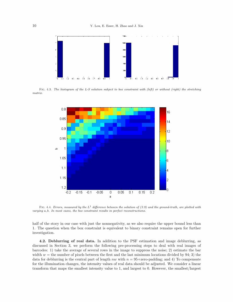
Box constraint. The original deblurring problem (3.8) is non-convex. People have noticed thatits global minimizer can often be obtained by solving the relaxed convex problem [6, 26]. Althoughthe box constraint does not explicitly enforce binary signal, the solution is almost binary. Figure 4.3plots the histogram of the LS solutions with and without the stretch matrix, both of which have twospikes at 0 and 1.

We further study the box constraint by deblurring with ground-truth PSF. The errors, measuredby the L1 difference between the solution of (3.9) and the ground-truth, are plotted in Figure 4.4 withvarying a and b. Depending on blur, the box constraint can give perfect reconstructions.

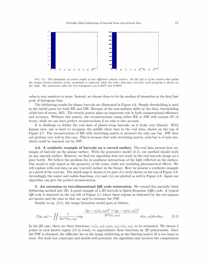
Our conjecture is that the LS solution with box constraint (3.9) is consistent with a binary solutionif the blurring matrix and the underlying signal satisfy certain conditions. Mao [26] proves that if His the selection of Fourier coefficients and certain number of low frequency coefficients are known, thenthe binary solution is the unique LS solution with box constraint. As H is a more general matrix inour case, we can not apply his analysis. For a general matrix, the exact l1 recovery of sparse solution isstudied in [11], in which the uniqueness condition depends on the coherence of the matrix. We plot thehistogram of cosine angles of two different column vectors. Two matrices are examined in Figure 4.5:one gives the unique binary solution if box constraint is enforced, and the other does not. We find twohistograms look similar, which suggests coherence is probably irrelevant to the equivalence betweenbox and binary constraint. In another related work [3], the authors prove that a sparse nonnegativesolution can be uniquely reconstructed as quadratic programming problem. This can be regarded as


Fig. 4.3. The histogram of the L-S solution subject to box constraint with (left) or without (right) the stretchingmatrix.

Fig. 4.4. Errors, measured by the L1 difference between the solution of (3.9) and the ground-truth, are plotted withvarying a, b. In most cases, the box constraint results in perfect reconstructions.

half of the story in our case with just the nonnegativity, as we also require the upper bound less than1. The question when the box constraint is equivalent to binary constraint remains open for furtherinvestigation.

4.2. Deblurring of real data. In addition to the PSF estimation and image deblurring, asdiscussed in Section 3, we perform the following pre-processing steps to deal with real images ofbarcodes: 1) take the average of several rows in the image to suppress the noise; 2) estimate the barwidth w = the number of pixels between the first and the last minimum locations divided by 94; 3) thedata for deblurring is the central part of length nw with n = 95+zero-padding; and 4) To compensatefor the illumination changes, the intensity values of real data should be adjusted. We consider a lineartransform that maps the smallest intensity value to 1, and largest to 0. However, the smallest/largest


Fig. 4.5. The histogram of cosine angles of two different column vectors. On the left is of the matrix that yieldsthe unique binary solution if box constraint is enforced, while the other that does not have such property is shown onthe right. The maximum value for two histograms are 0.9857 and 0.9989.

value is very sensitive to noise. Instead, we choose them to be the median of intensities at the first/lastpeak of histogram bins.

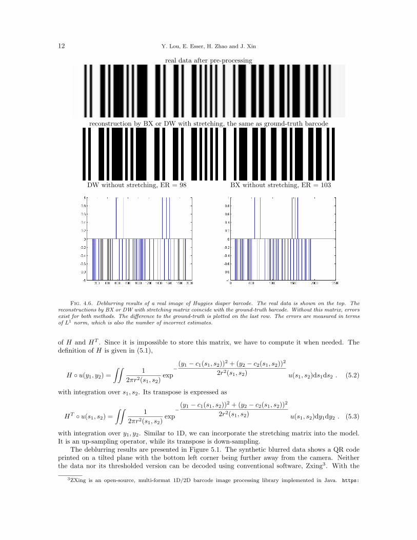
The deblurring results for diaper barcode are illustrated in Figure 4.6. Simple thresholding is usedas the initial guess for both BX and DW. Because of the non-uniform shifts in the data, thresholdingyields lots of errors, 30%. The stretch matrix plays an important role in both computational efficiencyand accuracy. Without this matrix, the reconstructions using either BX or DW still contain 3% oferrors, while we can have perfect reconstructions if we take it into account.

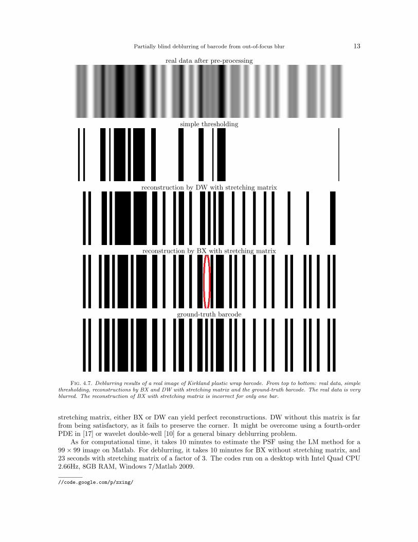
It is challenge to deblur the real data of plastic-wrap barcode, as it looks very blurred. Withhuman eyes, one is hard to recognize the middle three bars in the real data, shown on the top ofFigure 4.7. The reconstruction of BX with stretching matrix is incorrect for only one bar. DW doesnot perform very well in this case. This is because that with stretching matrix, each bar is of unit size,which could be smeared out by DW.

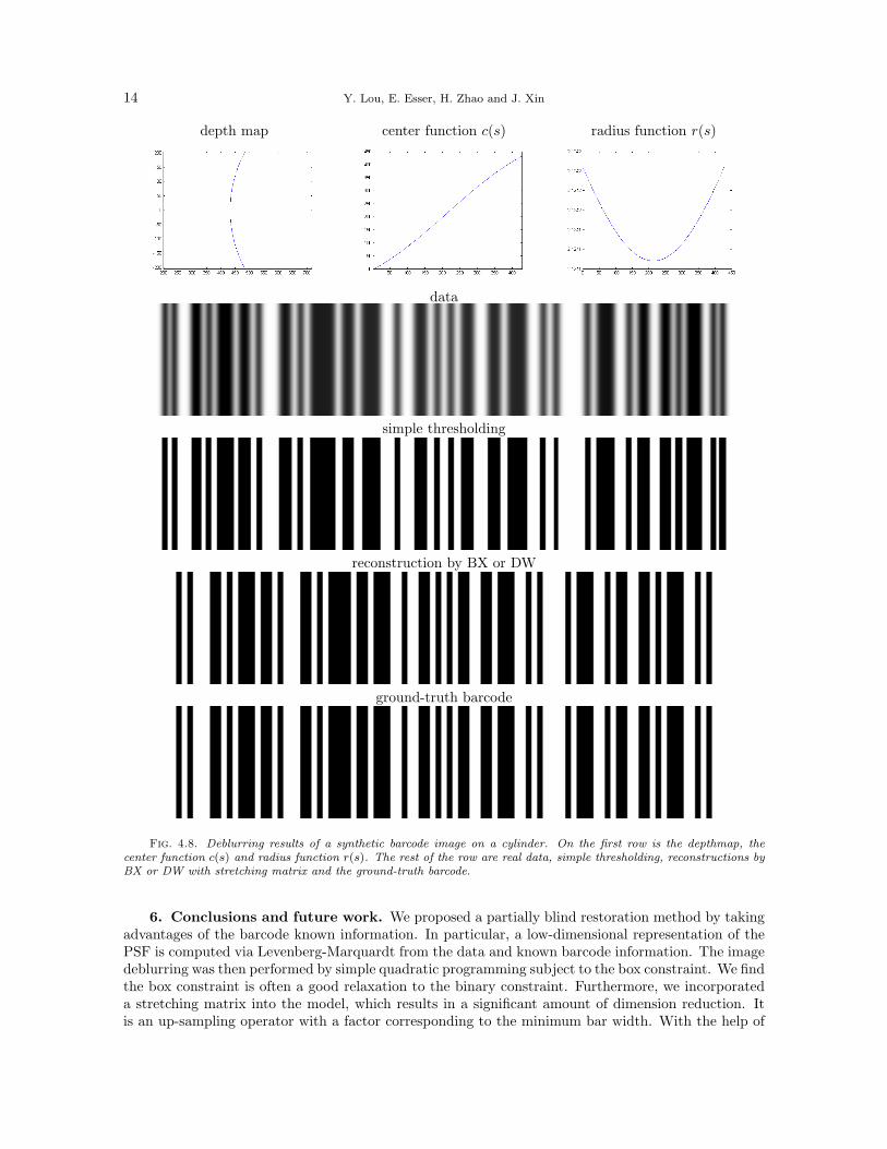
4.3. A synthetic example of barcode on a curved surface. The real data present here areimages of barcode on the planar surface. With the generative model (2.1), our method should workon any smooth surface. However, we find our algorithm does not work on the real barcode image on ajuice bottle. We believe the problem lies in nonlinear interactions of the light reflected on the surface.Our model is only aimed at the geometry of the scene, while not modeling photometrical effects. Wewill explore with real data on any (curved) surface in the future. Here we present a synthetic exampleas a proof of the concept. The depth map is chosen to be part of a circle shown on the top of Figure 4.8.Accordingly the center and radius functions, c(s) and r(s) are plotted as well in Figure 4.8. Again ouralgorithm can give the perfect reconstruction.

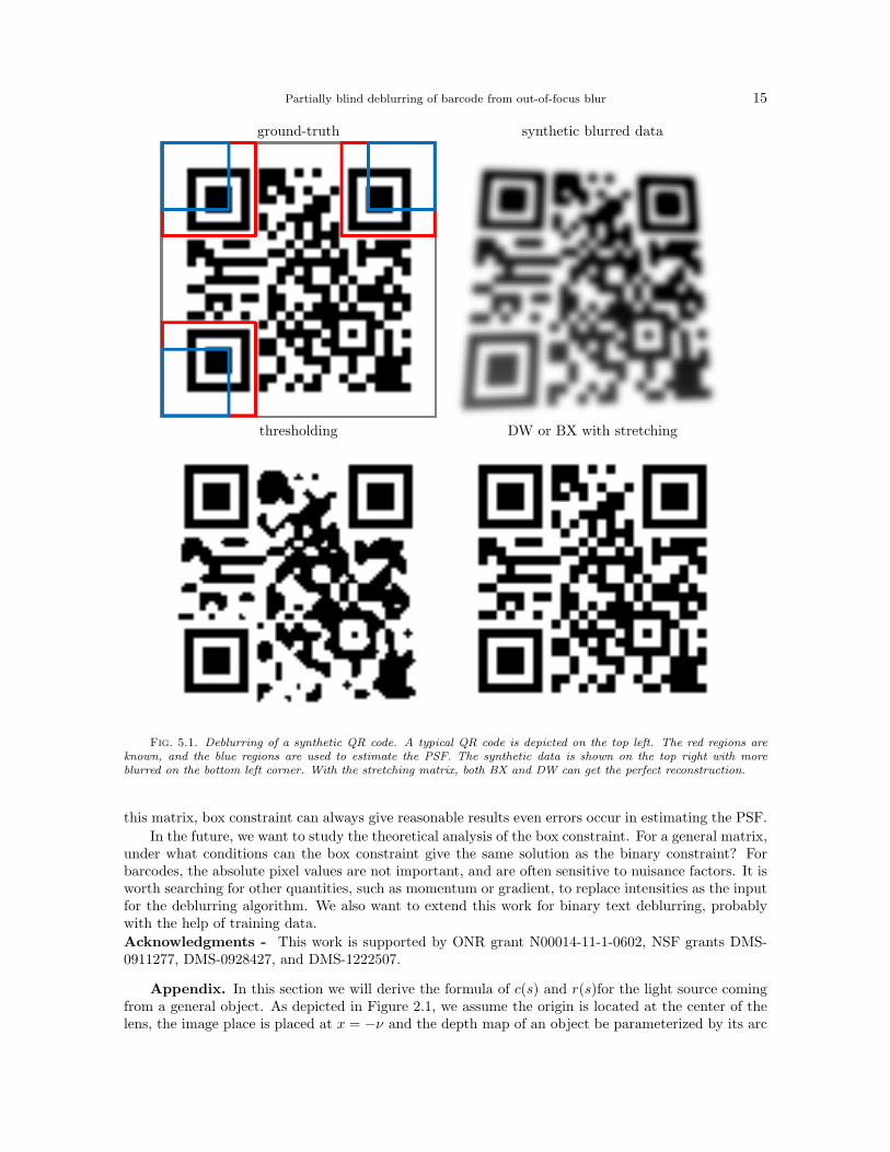
5. An extension to two-dimensional QR code restoration. We extend this partially blinddeblurring method into 2D. A good example of a 2D barcode is Quick Response (QR) code. A typicalQR code is depicted on the top left of Figure 5.1 where three regions as indicated by the red squaresare known and the ones in blue are used to estimate the PSF.

Similar to eq. (2.1), the image formation model goes as follows,

f(y1, y2) =∫∫

12πr2(s1, s2)

exp−

(y1 − c1(s1, s2))2 + (y2 − c2(s1, s2))2

2r2(s1, s2) u(s1, s2)ds1ds2 . (5.1)

In the 2D case, there are three functions, c1(s1, s2), c2(s1, s2), r(s1, s2), to be estimated. We choose 4points in each known region (12 in total), to approximate these functions by 2D polynomials. Oncethe PSF is obtained, the difficulty lies in the image deblurring as the blurring matrix H is too large tostore. For both box constraint and double-well potential, the algorithm only involves the computation


real data after pre-processing

reconstruction by BX or DW with stretching, the same as ground-truth barcode

DW without stretching, ER = 98 BX without stretching, ER = 103

Fig. 4.6. Deblurring results of a real image of Huggies diaper barcode. The real data is shown on the top. Thereconstructions by BX or DW with stretching matrix coincide with the ground-truth barcode. Without this matrix, errorsexist for both methods. The difference to the ground-truth is plotted on the last row. The errors are measured in termsof L1 norm, which is also the number of incorrect estimates.

of H and HT . Since it is impossible to store this matrix, we have to compute it when needed. Thedefinition of H is given in (5.1),

H u(y1, y2) =∫∫

12πr2(s1, s2)

exp−

(y1 − c1(s1, s2))2 + (y2 − c2(s1, s2))2

2r2(s1, s2) u(s1, s2)ds1ds2 . (5.2)

with integration over s1, s2. Its transpose is expressed as

HT u(s1, s2) =∫∫

12πr2(s1, s2)

exp−

(y1 − c1(s1, s2))2 + (y2 − c2(s1, s2))2

2r2(s1, s2) u(s1, s2)dy1dy2 . (5.3)

with integration over y1, y2. Similar to 1D, we can incorporate the stretching matrix into the model.It is an up-sampling operator, while its transpose is down-sampling.

The deblurring results are presented in Figure 5.1. The synthetic blurred data shows a QR codeprinted on a tilted plane with the bottom left corner being further away from the camera. Neitherthe data nor its thresholded version can be decoded using conventional software, Zxing3. With the

3ZXing is an open-source, multi-format 1D/2D barcode image processing library implemented in Java. https:


real data after pre-processing

simple thresholding

reconstruction by DW with stretching matrix

reconstruction by BX with stretching matrix

ground-truth barcode

Fig. 4.7. Deblurring results of a real image of Kirkland plastic wrap barcode. From top to bottom: real data, simplethresholding, reconstructions by BX and DW with stretching matrix and the ground-truth barcode. The real data is veryblurred. The reconstruction of BX with stretching matrix is incorrect for only one bar.

stretching matrix, either BX or DW can yield perfect reconstructions. DW without this matrix is farfrom being satisfactory, as it fails to preserve the corner. It might be overcome using a fourth-orderPDE in [17] or wavelet double-well [10] for a general binary deblurring problem.

As for computational time, it takes 10 minutes to estimate the PSF using the LM method for a99× 99 image on Matlab. For deblurring, it takes 10 minutes for BX without stretching matrix, and23 seconds with stretching matrix of a factor of 3. The codes run on a desktop with Intel Quad CPU2.66Hz, 8GB RAM, Windows 7/Matlab 2009.

//code.google.com/p/zxing/


depth map center function c(s) radius function r(s)

data

simple thresholding

reconstruction by BX or DW

ground-truth barcode

Fig. 4.8. Deblurring results of a synthetic barcode image on a cylinder. On the first row is the depthmap, thecenter function c(s) and radius function r(s). The rest of the row are real data, simple thresholding, reconstructions byBX or DW with stretching matrix and the ground-truth barcode.

6. Conclusions and future work. We proposed a partially blind restoration method by takingadvantages of the barcode known information. In particular, a low-dimensional representation of thePSF is computed via Levenberg-Marquardt from the data and known barcode information. The imagedeblurring was then performed by simple quadratic programming subject to the box constraint. We findthe box constraint is often a good relaxation to the binary constraint. Furthermore, we incorporateda stretching matrix into the model, which results in a significant amount of dimension reduction. Itis an up-sampling operator with a factor corresponding to the minimum bar width. With the help of


ground-truth synthetic blurred data

thresholding DW or BX with stretching

Fig. 5.1. Deblurring of a synthetic QR code. A typical QR code is depicted on the top left. The red regions areknown, and the blue regions are used to estimate the PSF. The synthetic data is shown on the top right with moreblurred on the bottom left corner. With the stretching matrix, both BX and DW can get the perfect reconstruction.

this matrix, box constraint can always give reasonable results even errors occur in estimating the PSF.In the future, we want to study the theoretical analysis of the box constraint. For a general matrix,

under what conditions can the box constraint give the same solution as the binary constraint? Forbarcodes, the absolute pixel values are not important, and are often sensitive to nuisance factors. It isworth searching for other quantities, such as momentum or gradient, to replace intensities as the inputfor the deblurring algorithm. We also want to extend this work for binary text deblurring, probablywith the help of training data.Acknowledgments - This work is supported by ONR grant N00014-11-1-0602, NSF grants DMS-0911277, DMS-0928427, and DMS-1222507.

Appendix. In this section we will derive the formula of c(s) and r(s)for the light source comingfrom a general object. As depicted in Figure 2.1, we assume the origin is located at the center of thelens, the image place is placed at x = −ν and the depth map of an object be parameterized by its arc


length parameter s 7→ (γ1(s), γ2(s)).The light source emitted from (γ1(s), γ2(s)) goes through the center of the lens and shades a disk

on the image plane. The center of this disk is the intersection of x = −ν and the line passing throughthe origin and (γ1(s), γ2(s)). Therefore, we have c(s) = −ν γ2(s)

γ1(s).

It follows from thin lens formula [19] that any light source at distance γ1(s) to the lens will focuson a plane with distance νs to the lens, which satisfies

1γ1(s)

+1νs

=1F

,

with F being the focal length of the camera. If ν 6= νs, then the image of this point depends on theboundary of the lens. Assuming a thin circular lens, a point of light produces a disk, whose radius canbe computed by simple similarity of triangles. The ratio between the radius of the disk and the radiusof the lens is equal to (ν − νs)/νs. Therefore, we have the radius function to be

r(s) =D

2

∣∣∣1− ν(1F− 1

γ1(s))∣∣∣

For barcode, it is often printed on a planar surface and thus its depth map is expressed as x = ay+b,whose arc length representation is

γ1(s) = s sin θ + bγ2(s) = s cos θ

(6.1)

for a = tan θ. Then we have

c(s) = −ν s cos θs sin θ+b = −νs

as+b√

a2+1

r(s) = D2 |1− ν( 1

F −√

a2+1as+b

√a2+1

)|(6.2)

If the plane is parallel to the lens, i.e. a = 0, then the center map c(s) = s after scaling. Theimage formation model (2.1) becomes the conventional shift-invariant blur.

REFERENCES

[1] M. Born and E. Wolf, Principles of Optics: Electromagnetic Theory of Propagation, Interference and Diffractionof Light (7th ed.), Cambridge: Cambridge University Press., 1999.

[2] A. M. Bronstein, A. M. Bronstein, M. Zibulevsky, and Y. Y. Zeevi, Blind deconvolution of images usingoptimal sparse representations, IEEE Transactions on Image Processing, 14 (2005), pp. 726–736.

[3] A. M. Bruckstein, M. Elad, and M. Zibulevsky, On the uniqueness of nonnegative sparse solutions to under-determined systems of equations, Information Theory, IEEE Transactions on, 54 (2008), pp. 4813 –4820.

[4] A. Chambolle and T. Pock, A first-order primal-dual algorithm for convex problems with applications to imaging,Journal of Mathematical Imaging and Vision, 40 (2011).

[5] S. H. Chan and T. Q. Nguyen, Single image spatially variant out-of-focus blur removal, in IEEE InternationalConference on Image Processing (ICIP), 2011, pp. 677–680.

[6] T. F. Chan, S. Esedoglu, and M. Nikolova, Algorithms for finding glboal minimizers of image segmentationand denoising models, SIAM J. Appl. Math., 66 (2006), pp. 1632–1648.

[7] T. F. Chan and C. K. Wong, Total variation blind deconvolution, IEEE Transactions on Image Processing, 7(1998), pp. 370 – 375.

[8] S. Cho, Y. Matsushita, and S. Lee, Removing non-uniform motion blur from images, in IEEE InternationalConference on Computer Vision (ICCV), Oct. 2007, pp. 1–8.

[9] R. Choksi and Y. van Gennip, Deblurring of one dimensional bar codes via total variation energy minimization,SIAM J. Img. Sci., 3 (2010), pp. 735–764.

[10] J. Dobrosotskaya and A. L. Bertozzi, Analysis of the wavelet Ginzburg-Landau energy in image applicationswith edges, SIAM J. Imaging Sciences, 6 (2013), pp. 698–729.

[11] D. L. Donoho and M. Elad, Optimally sparse representation in general (non-orthogonal) dictionaries via l1minimization, in Proc. Natl Acad. Sci. USA, vol. 100, 2003, pp. 2197–2202.

[12] S. Esedoglu, Blind deconvolution of bar code signals, Inverse Problems, 20 (2004), pp. 121–135.[13] E. Esser, X. Zhang, and T. F. Chan, A general framework for a class of first order primal-dual algorithms for

convex optimization in imaging science, SIAM J. Imag. Sci., 3 (2010), pp. 1015–1046.


[14] P. Favaro and S. Soatto, A geometric approach to shape from defocus, IEEE Transactions on Pattern Analysisand Machine Intelligence, 27 (2005), pp. 406–417.

[15] , 3-D Shape Estimation and Image Restoration: Exploiting Defocus and Motion Blur, Springer Verlag,December 2006.

[16] P. Favaro, S. Soatto, M. Burger, and S. Osher, Shape from defocus via diffusion, IEEE Transactions onPattern Analysis and Machine Intelligence, (2007).

[17] W. Gao and A. L. Bertozzi, Level set based multispectral segmentation with corners, SIAM J. Imag. Sci., 4(2011), pp. 597–617.

[18] B. He and X. Yuan, Convergence analysis of primal-dual algorithms for a saddle-point problem: From contractionperspective, SIAM J. Imaging Sciences, 5 (2012), pp. 119–149.

[19] E. Hecht, Optics (4th ed.), Addison Wesley, 2002.[20] M. A. Iwen, F. Santosa, and R. Ward, A symbol-based algorithm for decoding bar codes, SIAM J. Imaging Sci.,

6 (2013), p. 56C77.[21] J. Jia, Single image motion deblurring using transparency, in IEEE Conference on Computer Vision and Pattern

Recognition (CVPR), 2007.[22] E. Joseph and T. Pavlidis, Bar code wave-form recognition using peak locations, IEEE Trans. Pattern Anal.

Machine Intelligence, 16 (1994), pp. 630–640.[23] S. Kresic Juric, Edge detection in bar code signals corrupted by integrated time-varying speckle, Pattern Recog-

nition, 38 (2005), pp. 2483–2493.[24] D. Krishnan, T. Tay, and R. Fergus, Blind deconvolution using a normalized sparsity measure, in CVPR, 2011.[25] R. L. Lagendijk and J. Biemond, Basic methods for image restoration and identification, in Hand Book of image

and Vedio Processing, Alan C. Bovik, ed., Academic Press, 2000, pp. 125–140.[26] Y. Mao, Reconstruction of binary functions and shapes from incomplete frequency information, IEEE Trans. on

Information Theory, 58 (2012), pp. 3642–3653.[27] M.E. Moghaddam, A mathematical model to estimate out of focus blur, in International Symposium on Image

and Signal Processing and Analysis (ISPA), 2007, pp. 278–281.[28] J. G. Nagy and D. P. O’leary, Restoring images degraded by spatially variant blur, SIAM J. Sci. Comput., 19

(1998), pp. 1063–1082.[29] M. I. Sezan, G. Pavlovic, A. M. Tekalp, and A. T. Erdem, On modeling the focus blur in image restoration,

in Acoustics, Speech, and Signal Processing, International Conference on, vol. 4, 1991, pp. 2485 – 2488.[30] M. Zhu and T.F. Chan, An efficient primal-dual hybrid gradient algorithm for total variation image restoration,

tech. report, 2008. UCLA CAM Report [08-34].

Documents

PARTIALLY BLIND DEBLURRING OF BARCODE FROM …jxin/out_focus_blur_cam13-4… · · 2013-07-30PARTIALLY BLIND DEBLURRING OF BARCODE FROM OUT-OF-FOCUS BLUR YIFEI LOU, ERNIE ESSER,