Embed Size (px)
Citation preview
Partial Stochastic Analysis with the Aglink-Cosimo Model:
A Methodological Overview
Authors: Sergio René Araujo-Enciso, Simone Pieralli and Ignacio Pérez-Domínguez Editors: Simone Pieralli and Ignacio Pérez-Domínguez
2017
©WrightStudio – stock.adobe.com
EUR 28863 EN
2
This publication is a technical report by the Joint Research Centre (JRC), the European Commission’s science
and knowledge service. It aims to provide evidence-based scientific support to the European policymaking
process. The scientific output expressed does not imply a policy position of the European Commission. Neither
the European Commission nor any person acting on behalf of the Commission is responsible for the use that
might be made of this publication.
Contact information
Name: European Commission, Joint Research Centre (JRC), Directorate D — Sustainable Resources
Address: Edificio Expo. c/Inca Garcilaso, 3. E-41092 Seville (Spain)
Email: [email protected]
Tel.: +34 954488300
JRC Science Hub
https://ec.europa.eu/jrc
JRC108837
EUR 28863 EN
Print ISBN 978-92-79-76019-8 ISSN 1018-5593 doi:10.2760/450029
PDF ISBN 978-92-79-76018-1 ISSN 1831-9424 doi:10.2760/680976
Luxembourg: Publications Office of the European Union, 2017
© European Union, 2017
The reuse of the document is authorised, provided the source is acknowledged and the original meaning or
message of the texts are not distorted. The European Commission shall not be held liable for any consequences
stemming from the reuse.
How to cite this report: Araujo-Enciso, S.R., S. Pieralli, I. Pérez Domínguez, (2017): Partial Stochastic Analysis
with the Aglink-Cosimo Model: A Methodological Overview. JRC Technical Report, EUR 28863 EN,
doi:10.2760/680976
All images © European Union 2017, except: Front Page, by WrightStudio, Source: stock.adobe.com

3
Table of contents
Table of contents ................................................................................................... 3
List of tables ......................................................................................................... 4
List of figures ........................................................................................................ 4
Acknowledgements ................................................................................................ 5
Executive summary ............................................................................................... 6
1 Introduction ............................................................................................ 7
2 Methods for error extraction ...................................................................... 9
2.1 Regression of single model equations or equation systems .................................. 9
2.2 Methods for error extraction: cubic time trend fitting ....................................... 10
2.3 Methods for error extraction: vector autoregressive system of equations ............ 11
2.4 Testing for error extraction ........................................................................... 12
3 Methods for error simulation ................................................................... 14
3.1 Parametric approaches: multivariate normal or truncated multivariate normal
distribution functions ........................................................................................... 14
3.2 Semi-parametric approaches: empirical cumulative distribution functions and copulas 14
3.3 Methods for error simulation: testing for equality of simulated and true
uncertainty distributions ....................................................................................... 16
4 Methodology implementation and evaluation ............................................. 16
5 Results of the implementation ................................................................. 19
5.1 Selecting the best uncertainty extraction method ............................................ 19
5.2 Selecting the best uncertainty simulation method ............................................ 19
6 Implications for scenario analysis ............................................................. 25
6.1 Macroeconomic uncertainty ........................................................................... 25
6.2 Yield uncertainty .......................................................................................... 30
7 Implications of the proposed methodologies .............................................. 34
8 References ............................................................................................ 35

4
List of tables
Table 1. Proposed methodologies for the PSA: macroeconomic and yield uncertainty ... 17
Table 2. Number of variables with lowest MSE for the extraction of the uncertainty ..... 19
Table 3. Absolute number and proportion of rejections of the null hypothesis by the
KCD test at the 0.05 level of significance: yield uncertainty ........................ 20
Table 4. Absolute number and proportion of rejections of the null hypothesis by the
KCD test at the 0.05 level of significance: macroeconomic uncertainty ......... 21
Table 5. Main statistics for the variables of interest in the five macroeconomic
uncertainty methodologies ..................................................................... 27
Table 6. Deviation of average world price with respect to the baseline for the variables
of interest in the lower oil price scenario .................................................. 28
Table 7. Deviation of average world price with respect to the baseline for the variables
of interest in the high oil price scenario .................................................... 29
Table 8. Main statistics for the variables of interest in the three yield uncertainty
methodologies ...................................................................................... 30
Table 9. Deviation of the yield scenario with respect to the baseline for the variables
of interest ............................................................................................ 32
List of figures
Figure 1. Implementation for the method CBCNONPAR-YIELD using soft wheat yield
and producer price in the EU-13 as an example ........................................ 18
Figure 2. Distributions of the simulated uncertainty for oil prices ............................... 22
Figure 3. Uncertainty surrounding the oil price (per Brent barrel) for the projection
period:................................................................................................. 23
a) original method (OLSTRND-MACRO).................................................................... 23
b) VAR with yearly data non-parametric (VARYEARLYNONPAR) .................................. 23
Figure 4. Oil price spread indicating the high and low oil price scenarios/subsets for
each methodology ................................................................................. 25
Figure 5. Scatterplot for wheat yield uncertainty in Ukraine and Russia, cubic-
parametric and semi-parametric methods indicating subsets ...................... 32
5
Acknowledgements
We are grateful to the people who participated to the workshop on stochastics in April
2015 in Seville and, in particular, to those who contributed for their useful
methodological insights: Thomas Heckelei, Barry K. Goodwin, Ana Sanjuan López, Pat
Westhoff, Zebedee Nii-Nate Nartey, Fabien Santini and Graham Pilgrim. We also thank
Stefan Hubertus Gay, Jonathan Brooks, and Thomas Chatzopoulos for providing insight
and expertise that greatly assisted our research. We would also like to show our
gratitude to Ana Sanjuan López for some final comments that greatly improved this
report. Any remaining errors are our own and should not tarnish the reputations of
these esteemed persons.
6
Executive summary
Aglink-Cosimo is a recursive-dynamic partial equilibrium model developed and
maintained by the Organisation for Economic Co-operation and Development (OECD)
and the Food and Agriculture Organization of the United Nations (FAO) Secretariats as
a collaborative effort. The model is primarily used to prepare the OECD-FAO
Agricultural Outlook, a yearly publication aiming to provide baseline projections for the
main global agricultural commodities over the medium term. These deterministic
projections are enhanced by a partial stochastic analysis tool, which allows the analysis
of specific market uncertainties. This is done by producing counterfactual scenarios to
the baseline originating from varying yields and macroeconomic variables
stochastically.
The aim of this report is to propose and evaluate different methods of analysing
stochastically important yields and macroeconomic uncertainty drivers. In the first
stage, we identify and evaluate the best parametric method to extract unexplained
variability, which we consider to be uncertainty in the macroeconomic and yield
drivers. In the second stage, we test parametric and non-parametric methods side by
side to simulate 10 years of potentially different macroeconomic and yield
environments.
The results can be summarised as follows. For yields, we find that a parametric cubic
trend method performs best in the first stage and a non-parametric hierarchical copula
(Clayton) method is more appropriate in the second stage. For macroeconomic
variables, a vector autoregressive model performs best in the first stage, while a non-
parametric hierarchical copula (Frank) method is more appropriate in the second
stage.
7
1 Introduction
Aglink-Cosimo is a recursive-dynamic partial equilibrium model developed and
maintained by the Organisation for Economic Co-operation and Development (OECD)
and the Food and Agriculture Organization of the United Nations (FAO) Secretariats as
a collaborative effort. The model is primarily used to prepare the OECD-FAO
Agricultural Outlook, a yearly publication aiming to provide baseline projections for the
main global agricultural commodities over the medium term.
Aglink-Cosimo is a model widely used by countries that are members of both
organisations. Additionally, the countries or users engage in a broad range of model
development and improvement, in part to address the need for counterfactual policy
analysis. An example of that type of development is the partial stochastic analysis
(PSA) tool.
The PSA tool serves to assess a broad range of alternative scenarios, which diverge
from the baseline by treating a number of variables stochastically. The selection of
stochastic variables aims at identifying the major sources of uncertainty for EU
agricultural markets. In total, 39 country-specific macroeconomic variables, the crude
oil price, and 85 country- and product-specific yields are treated as uncertain within
this partial stochastic framework. Apart from the international oil price, four
macroeconomic variables are considered in specific countries: consumer price index
(CPI), gross domestic product index (GDPI), gross domestic product deflator (GDPD)
and exchange rate (XR). The countries considered are Australia, Brazil, Canada, China,
Europe, India, Japan, New Zealand, Russia, and United States. The yield variables are
key crop and milk yields in important world markets. Among the key crops, we include
wheat, barley, maize, oats, rye, rice, soybeans, rapeseeds, sunflower, palm oil, and
sugar beet and cane. Among the key markets, we include Europe, Kazakhstan,
Ukraine, Russia, Argentina, Brazil, Paraguay, Uruguay, Canada, Mexico, United States,
Indonesia, Malaysia, Thailand, Vietnam, Australia, China, India, and New Zealand. The
original methodology was developed by the European Commission Joint Research
Centre (JRC; formerly JRC-IPTS) based in Seville, with the collaboration of the
European Commission Directorate General for Agriculture and Rural Development (DG-
Agri). The methodology has gained attention over the years as it is useful in
developing scenarios in which uncertainty plays a key role (e.g. historical large yield
variability in important agricultural producers and exporters).
The PSA was first implemented in 2011. After preliminary contacts with the FAPRI
network in 2010-11, a workshop was organized in March 2011 by the JRC, DG AGRI
and DEFRA with the aim of implementing a stochastic methodology for uncertainty
analysis with Aglink-Cosimo inspired on the FAPRI work. This was done for the first
time for the EU Outlook in 2011-2021 (https://ec.europa.eu/agriculture/markets-and-
prices/medium-term-outlook_en) and culminated with the publication of a JRC
reference report (Burrell and Nii-Naate, 2013). Further methodological adjustments
were carried out on the occasion of the EU and OECD-FAO Outlook exercises of 2013
and 2014, with a switch to TROLL in 2013 for the computation of yield deviates and
the implementation of a multivariate truncation for both yields and macroeconomic
variables in 2014. At the time, macroeconomic uncertainty for some variables had to
be down-weighted in an ad-hoc manner to avoid explosive growth. Discussions and
brainstorming exercises on possible further improvements continued during 2013 and
2014 (e.g. iMAP Reference Group meeting of July 2014).
While the PSA tool is important for assessing the potential impact of selected sources
of uncertainty in the model, its results are conditional on the methods used for
extracting and simulating uncertainty. Previous methods, such as those employed by
8
Burrell and Nii-Naate (2013), have limitations that have been partially addressed by
making specific assumptions on the probabilistic distributions of the stochastic
variables during the simulation stage (e.g. normalisation or truncation). In order to
choose a certain methodology with scientific rigour, in April 2015 the JRC held an
expert workshop in Seville to discuss existing and potential methods. Several of the
recommendations made at that workshop have been considered in the work presented
in this report.
The aim of this report is to propose alternative methodologies for the PSA tool,
including some statistical approaches for evaluating it in a medium-term baseline
context and for analysing its performance when doing scenario analysis.
This report is organised as follows. After this introductory section, Section 2 provides
an overview of the methods used for extracting the yield and macroeconomic
uncertainty. Section 3 focuses on the methods used in simulating the uncertainty,
including the assumptions on the multivariate distributions. This third section closes
with a statistical test employed for verifying the quality of the simulations. Section 4
summarises the methodologies proposed based on the theoretical framework explained
in Sections 2 and 3. Section 5 explores the results of the statistical tests, aiming to
select the best methods. Section 6 focuses on the impact of each method using subset
scenarios. The report concludes with Section 7, in which final recommendations are
given, together with some caveats.
The stochastic process is mainly divided in two parts:
Error extraction (Part 1). ‘Residual errors’ are obtained from a specific method
(e.g. ordinary least squares (OLS) or seemingly unrelated regression (SUR))
applied to a particular estimation model specified (e.g. Aglink-Cosimo model,
cubic time trend, vector autoregressive panel regression).
Error simulation (Part 2). Based on the error extraction, a certain distribution of
errors around the baseline values is obtained.
Both sets of methodologies in Parts 1 and 2 can be paired depending on the selected
choice. Some of these combinations are presented in this report.
9
2 Methods for error extraction
The first step in the PSA is the extraction of the uncertainty from the target model
variables. When we speak about extracting or measuring uncertainty, we refer to past
uncertainty, which in a sense is a deviation from some expected outcome. This section
describes the methods used to extract that past uncertainty from the yield and the
macroeconomic variables, as well as a method for comparing which methodology
provides the best outcome.
2.1 Regression of single model equations or equation systems
The original methodology was developed by Burrell and Nii-Naate (2013). They
proposed calculating the uncertainty with the one-year-ahead projection error using
the deviation between the historical observations and the observations projected one
year in advance, as in equation (1):
𝑢𝑀𝐸𝑙𝑡 = 𝑀𝐸𝑙,𝑡𝐻 𝑀𝐸𝑙,𝑡−1
𝐵⁄ (1)
where 𝑀𝐸𝑙,𝑡𝐻 denotes the historical value of the variable in region l at time t and 𝑀𝐸
𝑙,𝑡 − 1𝐵
denotes the projected value for the variable in region l at the time t – 1. Yield
projections were taken from the model, whereas projections for macroeconomic
indicators originated from macroeconomic models produced by the European
Commission and other international agencies. This method is equivalent to considering
the ‘projection error’ as the uncertainty. Values were divided by the average of all the
observations and, therefore, standardised to a mean of 1. While this approach
provided a reasonable level of uncertainty for most of the yield and macroeconomic
variables, in cases of extreme historical observations, the distribution of the simulated
yield and macroeconomic variables included negative values.
In response to this concern, it was decided to calculate the yield uncertainty by means
of an OLS regression using the same structure of the model equation. This approach
considerably diminished the number of variables yielding negative values. However,
specific cases persisted. With regard to the macroeconomic variables, no model
equation allowed implementation of an OLS regression, as these variables are
exogenous in the Aglink-Cosimo model. As a result of this limitation, it was decided to
retain the original approach for extracting macroeconomic uncertainty and truncate the
distribution to eliminate negative values in a refinement of the methodology.
Performing estimations using the structure of Aglink-Cosimo has some costs in terms
of possible model revisions (e.g. splitting the coarse grains category into maize and
other coarse grains in the 2016 model version) or missing historical variables. The
version implemented in 2016 to draw errors consisted of fitting an OLS regression for
each equation. The most common equation for modelling yield in Aglink-Cosimo has
the following form:
𝐿𝑜𝑔(𝑌𝐿𝐷𝑐𝑙𝑡) = 𝑣𝑐𝑙 + 𝛿𝑌𝐿𝐷,𝑃𝑃,𝑐𝑙 ∙ 𝐿𝑜𝑔 (𝑃𝑃𝑐,𝑙,𝑡−1
𝜉𝐶𝑃𝐶𝐼𝐶𝑃𝐶𝐼𝑐𝑙𝑡−1+(1−𝜉𝐶𝑃𝐶𝐼)𝐶𝑃𝐶𝐼𝑐𝑙𝑡) + 𝛿𝑌𝐿𝐷,𝑇,𝑐𝑙 ∙ 𝑡 + 𝑢𝑐𝑙𝑡 (2)
where YLD corresponds to the dependent variable (i.e. yields in this case), PP is the
producer price deflated by the cost of production commodity index (CPCI), as defined
in the documentation of the Aglink-Cosimo EU module (Araujo-Enciso et al. 2015,
p. 16), c indicates the crop, l indicates the country or a region of the world where we
expect correlation among yields, u is a random error with zero mean and uncorrelated errors among each crop/country equation, t represents time, and 𝑣 and 𝛿's represent
coefficients to be estimated.
10
In this way, the extracted errors are equal to:
�̂�𝑐𝑙𝑡 = 𝐿𝑜𝑔(𝑌𝐿𝐷𝑐𝑙𝑡)−�̂�𝑐𝑙 − �̂�𝑌𝐿𝐷,𝑃𝑃,𝑐𝑙 ∙ 𝐿𝑜𝑔 (𝑃𝑃𝑐,𝑙,𝑡−1
𝜉𝐶𝑃𝐶𝐼𝐶𝑃𝐶𝐼𝑐𝑙𝑡−1+(1−𝜉𝐶𝑃𝐶𝐼)𝐶𝑃𝐶𝐼𝑐𝑙𝑡) − �̂�𝑌𝐿𝐷,𝑇,𝑐𝑙 ∙ 𝑡 (3)
where the accent on the components (˄) of this equation and of the following ones
denote predicted values.
An additional complexity is that, in several cases, yields are modelled in Aglink-Cosimo
following a different specification (e.g. Canadian wheat yields). In that case a linear
time trend was estimated as follows:
𝐿𝑜𝑔(𝑌𝐿𝐷𝑐𝑙𝑡) = 𝑣𝑐𝑙 + 𝛿𝑌𝐿𝐷,𝑇,𝑐𝑙 ∙ 𝑡 + 𝑢𝑐𝑙𝑡 (4)
It is important to bear in mind that with this simple OLS method no correlation is
considered between equations and, in principle, more variability is left unexplained.
The estimator used could be varied to be a SUR on blocks of equations where
correlations between yields in a region are considered. This means that we should
intuitively have lower uncertainty unexplained in the error term and in the simulation
of uncertainty. However, even if this SUR estimator works for some regions, the
correlation matrices are usually almost singular. Being almost singular means that the
model tries to estimate a system but the information of two independent variables is in
fact almost the same.
This problem could potentially be solved by including in the system of equations only
variables with largest explanatory power and by using their estimated variability also
for the other crops. This would, however, mean that the variability of one crop in a
region would be applied to other crops in the same region, which is difficult to justify.
In other words, it is cumbersome to attribute the measured variability of variables
included in the regression to any of the crops excluded from the regression because
collinearity problems.
We interpret these errors as the reproduction of past uncertainty in the future after
excluding what the model is able to explain. In other words, we expect not all visible
variability to be reproduced in future simulations but only the uncertainty that is not
explained by the fluctuations in the model. We know that the behaviour of the yield
variables is usually linear, thus, these results are in fact very similar to what can be
estimated by including only a flexible time trend.
2.2 Methods for error extraction: cubic time trend fitting
The second method is a simple method to extract the errors by means of a cubic time
trend. This method can be used for both yields and macroeconomic variables.
Moreover, it requires that the errors (i.e. the regression residuals) are obtained as
differences between the observed values and a fitted polynomial time trend of third
order. In other words, the errors are predicted as differences between observed and
predicted values.
The estimation model specified in this case is the following:
𝑌𝑐𝑙𝑡 = 𝑣𝑐𝑙 + 𝛼𝑐𝑙𝑡 + 𝛽𝑐𝑙𝑡2 + 𝛾𝑐𝑙𝑡3 + 𝑢𝑐𝑙𝑡 (5)
where Y represents the dependent variable, either yields or macroeconomic variables,
c indicates the variable, l indicates the country in a region of the world where we expect correlation among yields or macroeconomic variables, t represents time, and 𝑣
and 𝛼, 𝛽, 𝛾 represent parameters to be estimated.
11
The estimator used here is a SUR estimator. Given the inclusion of the same variables
as regressors, the use of a SUR estimator results in the same coefficients as in OLS. In
this way the extracted errors are equal to:
�̂�𝑐𝑙𝑡 = 𝑌𝑐𝑙𝑡 − �̂�𝑐𝑙 − �̂�𝑐𝑙𝑡 − �̂�𝑐𝑙𝑡2 − 𝛾𝑐𝑙𝑡3 (6)
We interpret these errors as a measure of past uncertainty in the future only after
taking into account a cubic time trend. In other words, we can expect that most
variability seen in the past would be reproduced in the simulations of future
uncertainty, except for the excluded cubic time trend.
2.3 Methods for error extraction: vector autoregressive system
of equations
The methods proposed in previous sections do not make any assumptions about long-
run relationships between variables. However, we believe that macroeconomic
variables influence each other. Therefore, neglecting such relationships could call into
question the credibility of the analysis. For this reason, a third method is proposed.
This method is slightly more complex: we extract the errors while considering the
dynamic nature of variables over time and the fact that there are long-run
relationships among variables in a certain region. A vector autoregression (VAR)
system of equations is a multi-equation model in which each endogenous variable
depends on its own historical observations and the other variables in the system. The
dynamic nature of the variables is considered because two lags are included among the
regressor variables (on the right-hand side). The number of lags may vary across
regions and could be determined by following a specific test (e.g. Akaike information
criterion, AIC 1 ). However, considering the length of the time series available for
analysis (18 time periods from 1997 to 2015), including more lags might decrease the
precision of the estimated coefficients. The correlation among variables, and thus
among equations, is considered because the two-years lags of the other regional
macroeconomic variables are included. Only the variables whose errors (uncertainty)
are correlated are considered.
The errors are obtained as differences between the observed values and a fitted model
where we include two lags in the system. These lagged variables capture much of the
correlation between macroeconomic variables in a region and of the variability of
macroeconomic variables over time. In other words, we expect the errors predicted to
be small and, thus, the ‘uncertainty’ included in the simulations (Part 2) to be lower
than in any of the previous methods presented. This lower amount of residual
uncertainty arises because we only leave the unexplained variability year over year: it
is similar to the unexplained portion of an autoregressive process.
For simplicity we include as an example the estimation model only with one-year lag.
The specification would be the following:
1 Lütkepohl (2004) provides a comprehensive overview of the most relevant selection criteria for
the time lag. Among the different options we have opted for the AIC because it allows comparing models with different number of parameters.

12
∆𝑌1𝑟𝑡 = 𝜔1𝑟𝑡 + 𝜍1𝑟𝑡−1∆𝑌1𝑟𝑡−1 + ⋯ + 𝜍1𝑟𝑡−1∆𝑌𝑀𝑟𝑡−1 + 𝜏1𝑟
⋮ ⋮ ⋮ ⋮∆𝑌𝑀𝑟𝑡 = 𝜔𝑀𝑟𝑡 + 𝜍𝑀𝑟𝑡−1∆𝑌1𝑟𝑡−1 + ⋯ + 𝜍𝑀𝑟𝑡−1∆𝑌𝑀𝑟𝑡−1 + 𝜏𝑀𝑟
(7)
∀𝑟 = 1, … , 𝑅;
where ∆𝑌1𝑟𝑡 represents the change from period t to t-1 in a dependent variable Y, M
indicates the macroeconomic variable (𝑚 = 1, … , 𝑀), r indicates a region (i.e. typically a
single country) of the world where we expect correlation among macroeconomic
variables, 𝜏 is a random error with zero mean and correlated standard errors across
variables, t represents time, and 𝜍's and 𝜔's represent parameters to be estimated.
In this way the extracted errors are equal, for each equation, to the following:
�̂�𝑚𝑟 = ∆𝑌𝑚𝑟𝑡 − �̂�𝑚𝑙𝑡 − 𝜍�̂�1𝑡−1∆𝑌𝑚1𝑡−1 − ⋯ − 𝜍�̂�𝑟𝑡−1∆𝑌𝑀𝑟𝑡−1 (8)
The equation systems related to the macroeconomic variables are estimated with
variables translated into growth rates and approximated by logarithmic differences.
This is because typically macroeconomic variables are non-stationary (i.e. they have a
unit root). For every country, one system with the following four macroeconomic
variables is estimated: consumer price index (CPI), gross domestic product index
(GDPI), gross domestic product deflator (GDPD) and exchange rate (XR).
The previous model includes macroeconomic indicators for only one country owing to
data limitations. Historically, yearly data are available for only a limited number of
years. If we were to include more countries, the number of parameters to estimate
would be larger than the number of observations. For this reason, we limit the model
to a country-reduced form.
As an alternative to such a reduced form, we could increase the number of
observations by using data with a different time frequency, for example quarterly data
from national sources. This would allow estimating the model as in equation (7),
including all countries simultaneously. However, this would have implications for the
uncertainty extraction as yearly deviations might differ from quarterly ones.
Note that we have selected a model with two lags. As mentioned before, it would be
preferable to test for the proper number of lags considering criteria such as the AIC.
However, the more lags we include, the more observations we lose from the
estimation. Eventually, this would lead to an uneven panel of estimated uncertainties
depending on the nature of the time series, which could cause problems in the
simulation.2
2.4 Testing for error extraction
After proposing alternative methodologies, we looked for a measure or indicator that
selects the best method. In principle, the maximum likelihood of the models as in
equations (2), (5) and (7) could be compared with a likelihood-ratio test, penalising
each model with the number of parameters or, alternatively, using the AIC. The
problem arises when comparing regression-based methods with a deterministic
calculation such as the model in equation (1). For this reason, we propose using a
2 We tested the AIC in various VARs with different numbers of time lags, ranging from one to three. As a result, we opted to homogenise all models and include two lags for each variable.
13
unified simple approach for all methods, such as the mean squared error (MSE), which
is defined as
𝑀𝑆𝐸 =1
𝑛∑ (�̂�𝑖 − 𝑌𝑖)
2𝑛𝑖=1 (9)
where �̂�𝑖 denotes either the fitted value from the models as equations (2), (5) and (7)
or the one-year-ahead projected value 𝑀�̂�𝑙,𝑡−1𝐵 , and 𝑌𝑖 denotes the true historical value.
The smaller the value of the MSE, the better the model extracts the uncertainty.
14
3 Methods for error simulation
The second step of the PSA is the simulation of the extracted uncertainty for the
medium-term outlook projection period. The simulation process relies on two core
assumptions: (i) the choice of a distribution for the extracted uncertainty and (ii) the
relationships among the exogenous uncertainties surrounding the variables of interest.
In this section we discuss alternative methods for simulating these errors in the future.
3.1 Parametric approaches: multivariate normal or truncated
multivariate normal distribution functions
The original methodology used in the PSA until 2016 relies on the assumption that the
error is normally distributed with mean equal to zero and constant standard deviation.
It is then possible to resample from the known distribution n times, knowing its
parameters (mean and standard deviation). One of the key choices for the PSA is the
relationships among the uncertainties surrounding the variables. For example,
uncertainty affecting yields that originates from weather shocks can affect
neighbouring areas in similar ways and with similar intensity.
For yields, the method simulating the uncertainty until 2016 assumes a parametric
probability density function (PDF), such as the multivariate truncated normal distribution (MTND), denoted 𝜓(𝝁, 𝚺, 𝒂, 𝒃; 𝒖), such that:
𝜓(𝝁, 𝚺, 𝒂, 𝒃; 𝒖) =exp{−
1
2(𝒖−𝝁)𝑇𝚺−𝟏(𝒖−𝝁)}
∫ exp{−1
2(𝒖−𝝁)𝑇𝚺−𝟏(𝒖−𝝁)}𝑑𝒖
𝑏𝑎
(10)
where 𝝁 denotes the mean of the extracted uncertainty vector 𝐮 , 𝚺 denotes the
covariance matrix and 𝐚 and 𝐛 are the low and high truncation points. Truncation is
needed to avoid negative or extreme cases. Thus, we select the truncation interval
such that is extends from half of the minimum to the maximum historical values of the
extracted errors. This has been done in an ad hoc manner to allow a degree of
negative skewness. In other words, we wanted to allow for a certain amount of
probability mass on the lower-tail side.
For macroeconomic variables, the method simulating the uncertainty assumed until
2016 a multivariate normal distribution (MND), avoiding truncation. The only exception
is the price of oil that is truncated owing to its large variability, which would otherwise
lead, in some cases, to negative values. For the non-truncated macroeconomic
variables, the denominator in equation (10) would be equal to 1 and the formula
becomes the numerator rescaled:
𝜓(𝝁, 𝚺; 𝒖) = −1
(2𝜋)𝑛/2|𝚺|1/2 exp {−1
2(𝒖 − 𝝁)𝑇𝚺−𝟏(𝒖 − 𝝁)} (11)
This methodology takes the residual errors from Part 1 (i.e. error extraction) and
constructs a covariance matrix and a vector average, which are used as distribution
parameters for a multivariate normal or truncated multivariate normal set of estimated
distributions.
3.2 Semi-parametric approaches: empirical cumulative distribution functions and copulas
The imposition of a parametric distribution family can be a source of concern as it will
shape the outcome of the simulations, especially if the assumed distribution function
does not replicate the true distribution. To address this concern, we propose the use of
15
semi-parametric methods. Specifically, we propose using an empirical cumulative
distribution function (ECDF), where no functional form is imposed on the uncertainty.
The ECDF is denoted 𝐹𝑛(𝑡) =1
𝑛∑ 1𝑥𝑖≤𝑡
𝑛𝑖=1 , where 1𝑥𝑖≤𝑡 is a Bernoulli random variable. The
ECDF is easily considered for univariate distributions, but application in multivariate
cases of more than two variables poses some challenges. To our knowledge, there are
not many examples that allow the simulation of our data directly from a multivariate
ECDF as well as goodness-of-fit tests. Thus, we turn our attention to copulas as an
alternative to capture the multiple relationships among the extracted uncertainties.
The original concept of copulas dates back to Sklar (1959) and has received attention
in empirical applications of joint distributions (Goodwin, 2015). A copula is defined as a
multivariate distribution function in the unit hypercube [0,1]P with uniform marginal
distributions such that
𝐶(𝑢1, 𝑢2, … 𝑢𝑝) = 𝐹 (𝐹1−1(𝑢1), … , 𝐹𝑝
−1(𝑢𝑝)) (12)
where 𝐹1(𝑢1), … , 𝐹𝑝(𝑢𝑝) are the univariate distributions. The density function of the
copula can be derived from equation (12) and the marginal density functions are as in
equation (13)
𝑐(𝑢1, 𝑢2, … 𝑢𝑝) =𝑓(𝐹1
−1(𝑢1),…,𝐹𝑝−1(𝑢𝑝))
∏ 𝑓(𝐹𝑖−1(𝑢𝑖))
𝑝𝑖=1
(13)
A broad range of copula types are available. The most frequently used copula types are
the elliptical and Archimedean copulas. The elliptical copulas include the Gaussian and
t copulas, both assuming linear relationship between the variables. However, whereas
the former imposes zero tail dependence, the latter only allows for symmetrical tail
dependence.
Some of the Archimedean copulas, like the Clayton copula, allow for asymmetrical tail
dependence. This representation is convenient when simulating a process in which
extreme events (e.g. unfavourable weather shocks) are more frequently occurring
together (e.g. bad yield in two competing crops in the same region). Each copula
family depicts a different type of dependency among variables. For example, the Frank
copula has no tail dependence, while the Clayton copula has low tail dependence.
However, Archimedean copulas represent the multivariate relationship, making use of
only one correlation parameter, which makes them quite restrictive.
In order to have a flexible system allowing different correlation values for each
bivariate relationship within a multiple framework, we propose using the hierarchical
Archimedean copula (HAC). The HAC is a system comprising nested bivariate copulas. For example, a three-variable system in an HAC 𝐶(𝑢1, 𝑢2, 𝑢3) with 𝑢2 and 𝑢3 nested
should be written as follows:
𝐶(𝑢1, 𝑢2, 𝑢3) = 𝐶𝐹0(𝑢1, 𝐶𝐹23
(𝑢2, 𝑢3)) = 𝐹0 (𝐹0−1(𝑢1) + 𝐹0
−1 (𝐹23(𝐹23−1(𝑢2) + 𝐹23
−1(𝑢3)))) (14)
The advantage of this type of copula is that it maintains flexibility for choosing a
marginal distribution. In this case, ECDFs can be used as marginal distributions. The
method is semi-parametric in the sense that the marginal density distribution is non-
parametric while the joint distribution has a functional form. While the copula can be
16
estimated using different measures of association, such as Pearson, Spearman or
Kendall, for the present methodology we selected the Kendall correlation rank.
Moreover, we selected the Clayton copula because it allows non-linear dependence in
the lower tail. Such an assumption can be understood to represent a stronger
correlation in the occurrence of bad weather events within a specific region. For the
macroeconomic variables we chose a Frank copula, since we assumed no tail dependence. The Clayton copula has a correlation parameter range equal to 𝜃 ∈
[−1,∞)\{0} , generator function 𝐹𝜃(𝑡) =1
𝜃(𝑡−𝜃 − 1) and generator inverse function
𝐹𝜃−1(𝑡) = (1 + 𝜃𝑡)−1
𝜃⁄ . The Frank copula has correlation parameter range 𝜃 ∈ ℝ\{0} ,
generator function 𝐹𝜃(𝑡) = −log (exp(−𝜃𝑡)−1
exp(−𝜃)−1) and generator inverse function 𝐹𝜃
−1(𝑡) =
−1
𝜃log(1 + exp(−𝑡)(exp(−𝜃) − 1)). The simulation with the HAC is implemented in the R
package HAC developed by Okhrin and Ristig (2014).
3.3 Methods for error simulation: testing for equality of simulated and true uncertainty distributions
The test used relates to marginal distributions and analyses whether the simulated
uncertainty distributions belong to the same family of the original uncertainty
distributions. In this case, we employed the non-parametric method developed by Li et
al. (2009) to test statistically if the densities proposed are the same. Such method is
implemented in the R package np, developed by Hayfield and Racine (2008). The test,
known as the kernel consistent density (KCD) test with mixed data types, is
constructed by taking the integrated square density differences for two variables. For
more details and the formulae, we refer the reader to the paper by Li et al. (2009).
4 Methodology implementation and evaluation
After providing a theoretical background of the proposed methods, we proceed to their
implementation and evaluation.
For the yield uncertainty extraction and estimation, we propose two new
methodologies in addition to the original.
The first method is called cubic-parametric (CBCPAR-YIELD). It consists of
extracting the error by de-trending the yield with a cubic polynomial as in
equation (5) and, successively, in simulating the uncertainty via a multivariate
truncated normal distribution as in equation (10).
The second method is called cubic-nonparametric (CBCNONPAR-YIELD). In the
second method we also de-trend the yield with a cubic polynomial as in
equation (5), but the uncertainty is simulated assuming a marginal empirical
cumulative distribution function with a HAC joint distribution as in equation
(12).
These two new methodologies are compared with the original methodology where the
yield is de-trended as in equation (2) and then the uncertainty simulated with a
multivariate truncated normal distribution as in equation (10). This is what we term
the OLSTRND-YIELD method.
Uncertainty in macroeconomic variables poses more challenges than in the case of
yields. Here, we propose a total of four new methodologies.
First we propose a cubic-parametric methodology (CBCPAR-MACRO). It consists
of de-trending the macroeconomic variables with a cubic polynomial as in
17
equation (5), and then simulating the uncertainty with a multivariate normal
distribution as in equation (10).
The second method is called cubic-nonparametric macroeconomic methodology
(CBCNONPAR-MACRO). It uses a cubic polynomial to de-trend the variables in
the error extraction phase as in equation (5) and then uses a marginal ECDF
and a HAC joint distribution to simulate the errors in the future as in
equation (12).
The next two methods extract the uncertainty with a VAR in the error extraction
phase. These methods employ yearly data. In the simulation phase, we employ
parametric (assuming a MND) and non-parametric (assuming a marginal ECDF
and a HAC joint distribution) simulation methods obtaining two alternatives,
called, respectively, VARYEARLYPAR and VARYEARLYNONPAR.
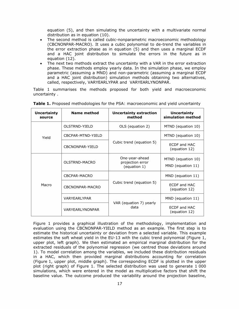
Table 1 summarises the methods proposed for both yield and macroeconomic
uncertainty .
Table 1. Proposed methodologies for the PSA: macroeconomic and yield uncertainty
Uncertainty source
Name method Uncertainty extraction method
Uncertainty simulation method
Yield
OLSTRND-YIELD OLS (equation 2) MTND (equation 10)
CBCPAR-MTND-YIELD
Cubic trend (equation 5)
MTND (equation 10)
CBCNONPAR-YIELD ECDF and HAC (equation 12)
Macro
OLSTRND-MACRO
One-year-ahead
projection error
(equation 1)
MTND (equation 10)
MND (equation 11)
CBCPAR-MACRO
Cubic trend (equation 5)
MND (equation 11)
CBCNONPAR-MACRO ECDF and HAC (equation 12)
VARYEARLYPAR
VAR (equation 7) yearly
data
MND (equation 11)
VARYEARLYNONPAR ECDF and HAC (equation 12)
Figure 1 provides a graphical illustration of the methodology, implementation and
evaluation using the CBCNONPAR-YIELD method as an example. The first step is to
estimate the historical uncertainty or deviation from a selected variable. This example
estimates the soft wheat yield in the EU-13 with the cubic trend polynomial (Figure 1,
upper plot, left graph). We then estimated an empirical marginal distribution for the
extracted residuals of the polynomial regression (we centred those deviations around
1). To model correlation among the variables, we included these distribution residuals
in a HAC, which then provided marginal distributions accounting for correlation
(Figure 1, upper plot, middle graph). The corresponding ECDF is plotted in the upper
plot (right graph) of Figure 1. The selected distribution was used to generate 1 000
simulations, which were entered in the model as multiplicative factors that shift the
baseline value. The outcome produced the variability around the projection baseline,

18
having as model past uncertainty (Figure 1, middle plot). Finally, the 1 000 values for
the uncertainty served to solve the Aglink-Cosimo model 1 000 times. In this example,
we show the distribution of EU-13 soft wheat producer price, resulting from the 1 000
solutions (Figure 1, lower plot). The range of endogenous solutions can be obtained to
observe the impact of uncertainty on the endogenous price response.
Figure 1. Implementation for the method CBCNONPAR-YIELD using soft wheat yield and producer price in the EU-13 as an example
19
5 Results of the implementation
This section summarises the results of the statistical methods and tests implemented
for evaluating the yield and macroeconomic uncertainty estimates in the extraction and
simulation steps of the PSA.
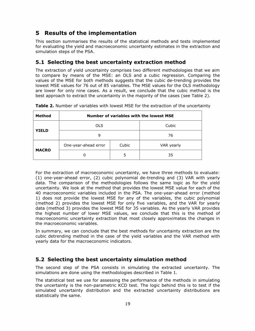
5.1 Selecting the best uncertainty extraction method
The extraction of yield uncertainty comprises two different methodologies that we aim
to compare by means of the MSE: an OLS and a cubic regression. Comparing the
values of the MSE for both methods suggests that the cubic de-trending provides the
lowest MSE values for 76 out of 85 variables. The MSE values for the OLS methodology
are lower for only nine cases. As a result, we conclude that the cubic method is the
best approach to extract the uncertainty in the majority of the cases (see Table 2).
Table 2. Number of variables with lowest MSE for the extraction of the uncertainty
Method Number of variables with the lowest MSE
YIELD
OLS Cubic
9 76
MACRO
One-year-ahead error Cubic VAR yearly
0 5 35
For the extraction of macroeconomic uncertainty, we have three methods to evaluate:
(1) one-year-ahead error, (2) cubic polynomial de-trending and (3) VAR with yearly
data. The comparison of the methodologies follows the same logic as for the yield
uncertainty. We look at the method that provides the lowest MSE value for each of the
40 macroeconomic variables included in the PSA. The one-year-ahead error (method
1) does not provide the lowest MSE for any of the variables, the cubic polynomial
(method 2) provides the lowest MSE for only five variables, and the VAR for yearly
data (method 3) provides the lowest MSE for 35 variables. As the yearly VAR provides
the highest number of lower MSE values, we conclude that this is the method of
macroeconomic uncertainty extraction that most closely approximates the changes in
the macroeconomic variables.
In summary, we can conclude that the best methods for uncertainty extraction are the
cubic detrending method in the case of the yield variables and the VAR method with
yearly data for the macroeconomic indicators.
5.2 Selecting the best uncertainty simulation method
The second step of the PSA consists in simulating the extracted uncertainty. The
simulations are done using the methodologies described in Table 1.
The statistical test we use for assessing the performance of the methods in simulating
the uncertainty is the non-parametric KCD test. The logic behind this is to test if the
simulated uncertainty distribution and the extracted uncertainty distributions are
statistically the same.
20
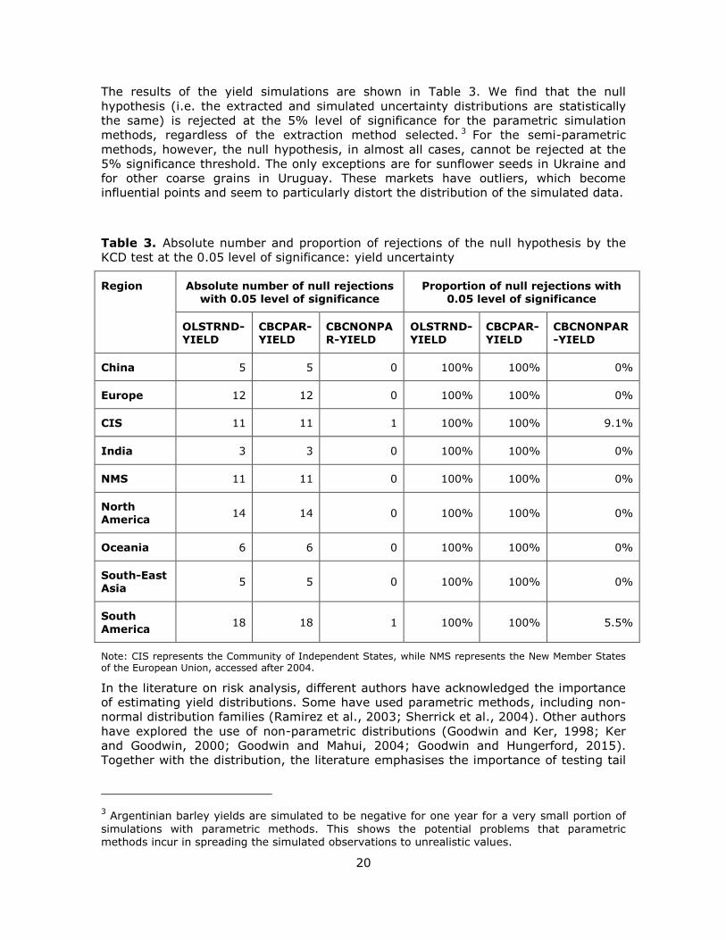
The results of the yield simulations are shown in Table 3. We find that the null
hypothesis (i.e. the extracted and simulated uncertainty distributions are statistically
the same) is rejected at the 5% level of significance for the parametric simulation
methods, regardless of the extraction method selected. 3 For the semi-parametric
methods, however, the null hypothesis, in almost all cases, cannot be rejected at the
5% significance threshold. The only exceptions are for sunflower seeds in Ukraine and
for other coarse grains in Uruguay. These markets have outliers, which become
influential points and seem to particularly distort the distribution of the simulated data.
Table 3. Absolute number and proportion of rejections of the null hypothesis by the
KCD test at the 0.05 level of significance: yield uncertainty
Region Absolute number of null rejections
with 0.05 level of significance
Proportion of null rejections with
0.05 level of significance
OLSTRND-YIELD
CBCPAR-YIELD
CBCNONPAR-YIELD
OLSTRND-YIELD
CBCPAR-YIELD
CBCNONPAR-YIELD
China 5 5 0 100% 100% 0%
Europe 12 12 0 100% 100% 0%
CIS 11 11 1 100% 100% 9.1%
India 3 3 0 100% 100% 0%
NMS 11 11 0 100% 100% 0%
North America
14 14 0 100% 100% 0%
Oceania 6 6 0 100% 100% 0%
South-East Asia
5 5 0 100% 100% 0%
South
America 18 18 1 100% 100% 5.5%
Note: CIS represents the Community of Independent States, while NMS represents the New Member States of the European Union, accessed after 2004.
In the literature on risk analysis, different authors have acknowledged the importance
of estimating yield distributions. Some have used parametric methods, including non-
normal distribution families (Ramirez et al., 2003; Sherrick et al., 2004). Other authors
have explored the use of non-parametric distributions (Goodwin and Ker, 1998; Ker
and Goodwin, 2000; Goodwin and Mahui, 2004; Goodwin and Hungerford, 2015).
Together with the distribution, the literature emphasises the importance of testing tail
3 Argentinian barley yields are simulated to be negative for one year for a very small portion of
simulations with parametric methods. This shows the potential problems that parametric methods incur in spreading the simulated observations to unrealistic values.
21
dependence and the accuracy of the selected copula. In the literature, we did not find
implementation of a test that allows us to discern the different types of copulas for the
HAC approach. Alternatively, we could use Vine copulas, which allow direct comparison
of the structures selected with a maximum likelihood test. However, such approach
requires large datasets to estimate and perform the tests. In addition, the selection of
the model within the vine copulas method, relies on the order of the variables and
marginal distribution functional forms, which are chosen based on expert knowledge.
Being aware of the sample size we have, rather than attempting to estimate a set of
complex relationships involving functional forms and non-parametric kernel
distributions, we opted to implement the HAC method with an empirical distribution,
which is a straightforward alternative free of distributional assumptions. The outcome
of the KCD test suggests that the choice of the ECDF provides simulations that
resemble the true distribution of the uncertainty.
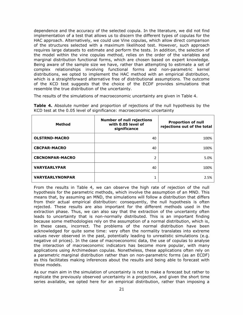
The results of the simulations of macroeconomic uncertainty are given in Table 4.
Table 4. Absolute number and proportion of rejections of the null hypothesis by the
KCD test at the 0.05 level of significance: macroeconomic uncertainty
Method Number of null rejections
with 0.05 level of significance
Proportion of null rejections out of the total
OLSTRND-MACRO 40 100%
CBCPAR-MACRO 40 100%
CBCNONPAR-MACRO 2 5.0%
VARYEARLYPAR 40 100%
VARYEARLYNONPAR 1 2.5%
From the results in Table 4, we can observe the high rate of rejection of the null
hypothesis for the parametric methods, which involve the assumption of an MND. This
means that, by assuming an MND, the simulations will follow a distribution that differs
from their actual empirical distribution: consequently, the null hypothesis is often
rejected. These results are also important for the different methods used in the
extraction phase. Thus, we can also say that the extraction of the uncertainty often
leads to uncertainty that is non-normally distributed. This is an important finding
because some methodologies rely on the assumption of a normal distribution, which is,
in these cases, incorrect. The problems of the normal distribution have been
acknowledged for quite some time: very often the normality translates into extreme
values never observed in the past, potentially leading to unrealistic simulations (e.g.
negative oil prices). In the case of macroeconomic data, the use of copulas to analyse
the interaction of macroeconomic indicators has become more popular, with many
applications using Archimedean copulas. Nonetheless, these applications often rely on
a parametric marginal distribution rather than on non-parametric forms (as an ECDF)
as this facilitates making inferences about the results and being able to forecast with
those models.
As our main aim in the simulation of uncertainty is not to make a forecast but rather to
replicate the previously observed uncertainty in a projection, and given the short time
series available, we opted here for an empirical distribution, rather than imposing a
22
functional form. The outcome of the KCD test confirmed our assumptions. For
simulating the uncertainty using short time series, it is better to use the empirical
distributions as this will avoid introducing bias in the results.
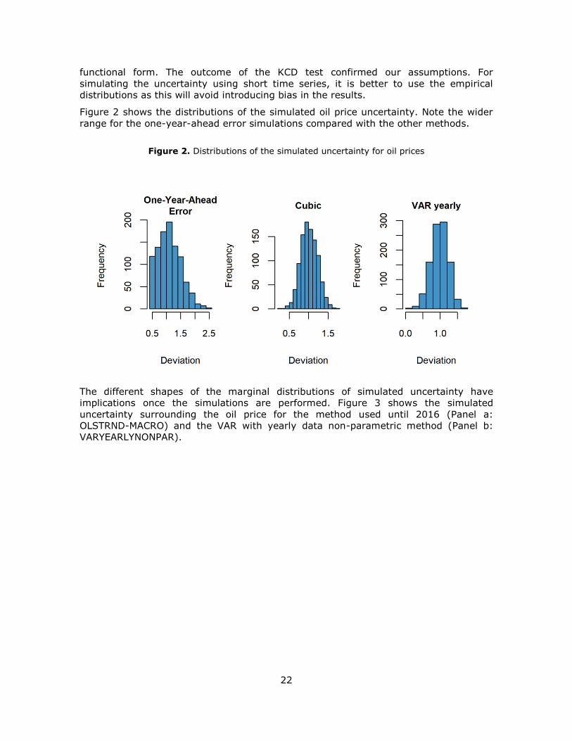
Figure 2 shows the distributions of the simulated oil price uncertainty. Note the wider
range for the one-year-ahead error simulations compared with the other methods.
Figure 2. Distributions of the simulated uncertainty for oil prices
The different shapes of the marginal distributions of simulated uncertainty have
implications once the simulations are performed. Figure 3 shows the simulated
uncertainty surrounding the oil price for the method used until 2016 (Panel a:
OLSTRND-MACRO) and the VAR with yearly data non-parametric method (Panel b:
VARYEARLYNONPAR).

23
Figure 3. Uncertainty surrounding the oil price (per Brent barrel) for the projection period:
a) original method (OLSTRND-MACRO)
b) VAR with yearly data non-parametric (VARYEARLYNONPAR)
Both pictures offer a clear view of the effect that the different methodologies have on
uncertainty. The original method allows large deviation from the baseline in the high
percentiles (top 2.5%) of the simulations while the lower percentiles are more
uniformly distributed than in the non-parametric method. On the other hand, the non-
parametric method provides lower dispersion of extremely high prices and slightly
more dispersed prices lower than the baseline.
After evaluating both stages of the PSA methodology (extraction and simulation), the
conclusions are as follows. For yields, we recommend performing the extraction with a
cubic time trend and the simulation with a semi-parametric copula (empirical marginal
and Clayton copula). For macroeconomic variables, we recommend performing the

24
uncertainty extraction with a VAR and the uncertainty simulation with a semi-
parametric copula (empirical marginal and Frank copula).
25
6 Implications for scenario analysis
While the MSE and KCD tests allow ranking of the methods for extracting and
simulating uncertainty, it is useful to examine how the different proposed methods can
influence the scenario analysis. Therefore, we turn our attention to evaluating the
possible impact of the different methodologies on a predefined set of scenarios.
One of the most common analyses carried out to study the implications of uncertainty
is the ‘subset analysis’. As its name indicates, it is based on a subsample of the
stochastic simulations of the model. The simulations contained in the subset can be
selected with a different number of criteria. For the purpose of this evaluation, we have
developed two scenarios, one for macroeconomic uncertainty and another for yield
uncertainty.
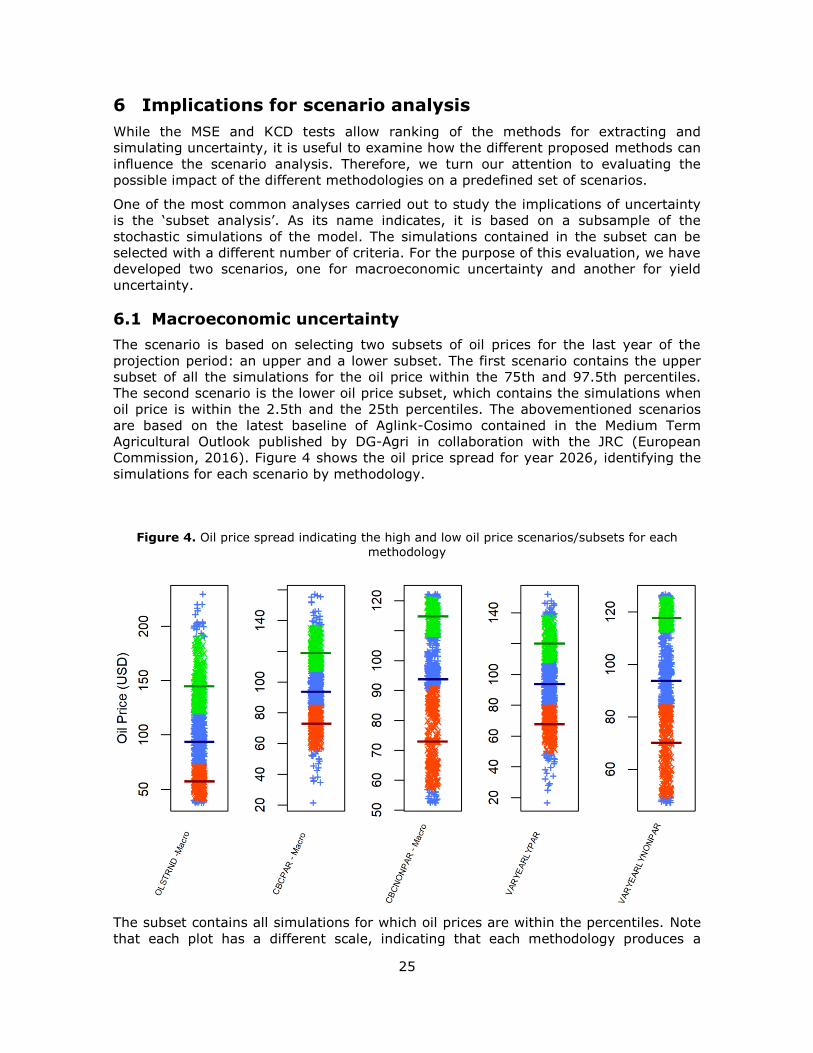
6.1 Macroeconomic uncertainty
The scenario is based on selecting two subsets of oil prices for the last year of the
projection period: an upper and a lower subset. The first scenario contains the upper
subset of all the simulations for the oil price within the 75th and 97.5th percentiles.
The second scenario is the lower oil price subset, which contains the simulations when
oil price is within the 2.5th and the 25th percentiles. The abovementioned scenarios
are based on the latest baseline of Aglink-Cosimo contained in the Medium Term
Agricultural Outlook published by DG-Agri in collaboration with the JRC (European
Commission, 2016). Figure 4 shows the oil price spread for year 2026, identifying the
simulations for each scenario by methodology.
Figure 4. Oil price spread indicating the high and low oil price scenarios/subsets for each
methodology
The subset contains all simulations for which oil prices are within the percentiles. Note
that each plot has a different scale, indicating that each methodology produces a
26
different range of prices. Simulations corresponding to the low oil price subset are in
red, simulations within the high oil price subset are in green and the remainder are in
blue. The blue dots below and above the subsets correspond to the 0th–2.5th and
97.5th–100th percentiles. The bold lines in green and red represent the average of the
high and low oil price subset, respectively, and the blue line is the baseline.
Because it would be cumbersome to analyse all the variables in the model, we restrict
the analysis to those variables more likely to be affected directly and indirectly by
stochastic shocks. The world prices are the ideal variables for these types of scenario
because the world price clearing mechanism in the model accounts for the adjustments
in domestic markets and trade.4 Domestic markets are affected by oil prices directly on
the supply side, thus causing movements of the domestic market balance and the
domestic prices. The overall adjustment of all domestic markets is reflected in the
world price deviations from the baseline.
Before analysing the impact of the stochastic methodologies in the subsets, it is useful
to consider the main statistics of the variables of interest (world prices), obtained by
solving Aglink-Cosimo using different methods. The results are summarised in Table 5.
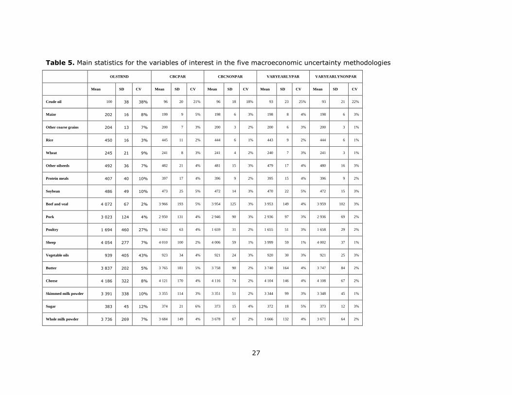
Table 5 shows the mean, standard deviation (SD) and coefficient of variation (CV) for
the five methodologies (these statistics consider the whole sample). With regard to the
average world prices, the original methodology has the largest values, followed by the
cubic polynomial methods (both parametric and semi-parametric) and, finally, the
VAR. We notice that same uncertainty extraction methods have a similar mean for all
the variables of interest. Nonetheless, the SD is different and the pattern we observe is
a lower SD value for the semi-parametric methods. Such an outcome confirms our
previous hypothesis: imposing normality leads to simulation of extreme cases never
observed in the historical data. In turn, those outliers are responsible for a larger SD in
the parametric methods. The other interesting finding regarding the CV is that its
values are lower for the cubic trend methodologies, followed by the VAR and then by
the year-ahead-error projection (i.e. original) method. While the year-ahead-error
projection has the largest CV, and can potentially have a broader range of results, this
methodology includes bias from imposing normality and does not properly detrend past
variation, but rather it is influenced by how good or bad the projection of the
macroeconomic indicators has been in the past.
4 Aglink-Cosimo has a market clearance mechanism for the world markets for the following
commodities: wheat, maize, coarse grains, rice, soybean, other oilseeds, sugar, vegetable oil, protein meals, pork meat, beef and veal meat, poultry, butter, cheese, skimmed milk powder and whole milk powder.
27
Table 5. Main statistics for the variables of interest in the five macroeconomic uncertainty methodologies
OLSTRND CBCPAR CBCNONPAR VARYEARLYPAR VARYEARLYNONPAR
Mean SD CV Mean SD CV Mean SD CV Mean SD CV Mean SD CV
Crude oil 100 38 38% 96 20 21% 96 18 18% 93 23 25% 93 21 22%
Maize 202 16 8% 199 9 5% 198 6 3% 198 8 4% 198 6 3%
Other coarse grains 204 13 7% 200 7 3% 200 3 2% 200 6 3% 200 3 1%
Rice 450 16 3% 445 11 2% 444 6 1% 443 9 2% 444 6 1%
Wheat 245 21 9% 241 8 3% 241 4 2% 240 7 3% 241 3 1%
Other oilseeds 492 36 7% 482 21 4% 481 15 3% 479 17 4% 480 16 3%
Protein meals 407 40 10% 397 17 4% 396 9 2% 395 15 4% 396 9 2%
Soybean 486 49 10% 473 25 5% 472 14 3% 470 22 5% 472 15 3%
Beef and veal 4 072 67 2% 3 966 193 5% 3 954 125 3% 3 953 149 4% 3 959 102 3%
Pork 3 023 124 4% 2 950 131 4% 2 946 90 3% 2 936 97 3% 2 936 69 2%
Poultry 1 694 460 27% 1 662 63 4% 1 659 31 2% 1 655 51 3% 1 658 29 2%
Sheep 4 054 277 7% 4 010 100 2% 4 006 59 1% 3 999 59 1% 4 002 37 1%
Vegetable oils 939 405 43% 923 34 4% 921 24 3% 920 30 3% 921 25 3%
Butter 3 837 202 5% 3 765 181 5% 3 758 90 2% 3 740 164 4% 3 747 84 2%
Cheese 4 186 322 8% 4 121 170 4% 4 116 74 2% 4 104 146 4% 4 108 67 2%
Skimmed milk powder 3 391 338 10% 3 355 114 3% 3 351 51 2% 3 344 99 3% 3 348 45 1%
Sugar 383 45 12% 374 21 6% 373 15 4% 372 18 5% 373 12 3%
Whole milk powder 3 736 269 7% 3 684 149 4% 3 678 67 2% 3 666 132 4% 3 671 64 2%
28
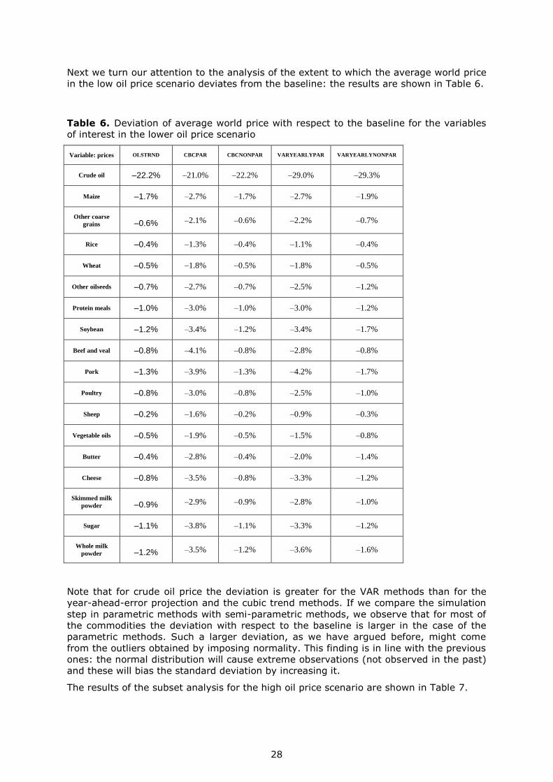
Next we turn our attention to the analysis of the extent to which the average world price
in the low oil price scenario deviates from the baseline: the results are shown in Table 6.
Table 6. Deviation of average world price with respect to the baseline for the variables
of interest in the lower oil price scenario
Variable: prices OLSTRND CBCPAR CBCNONPAR VARYEARLYPAR VARYEARLYNONPAR
Crude oil –22.2% –21.0% –22.2% –29.0% –29.3%
Maize –1.7% –2.7% –1.7% –2.7% –1.9%
Other coarse
grains –0.6% –2.1% –0.6% –2.2% –0.7%
Rice –0.4% –1.3% –0.4% –1.1% –0.4%
Wheat –0.5% –1.8% –0.5% –1.8% –0.5%
Other oilseeds –0.7% –2.7% –0.7% –2.5% –1.2%
Protein meals –1.0% –3.0% –1.0% –3.0% –1.2%
Soybean –1.2% –3.4% –1.2% –3.4% –1.7%
Beef and veal –0.8% –4.1% –0.8% –2.8% –0.8%
Pork –1.3% –3.9% –1.3% –4.2% –1.7%
Poultry –0.8% –3.0% –0.8% –2.5% –1.0%
Sheep –0.2% –1.6% –0.2% –0.9% –0.3%
Vegetable oils –0.5% –1.9% –0.5% –1.5% –0.8%
Butter –0.4% –2.8% –0.4% –2.0% –1.4%
Cheese –0.8% –3.5% –0.8% –3.3% –1.2%
Skimmed milk
powder –0.9% –2.9% –0.9% –2.8% –1.0%
Sugar –1.1% –3.8% –1.1% –3.3% –1.2%
Whole milk
powder –1.2% –3.5% –1.2% –3.6% –1.6%
Note that for crude oil price the deviation is greater for the VAR methods than for the
year-ahead-error projection and the cubic trend methods. If we compare the simulation
step in parametric methods with semi-parametric methods, we observe that for most of
the commodities the deviation with respect to the baseline is larger in the case of the
parametric methods. Such a larger deviation, as we have argued before, might come
from the outliers obtained by imposing normality. This finding is in line with the previous
ones: the normal distribution will cause extreme observations (not observed in the past)
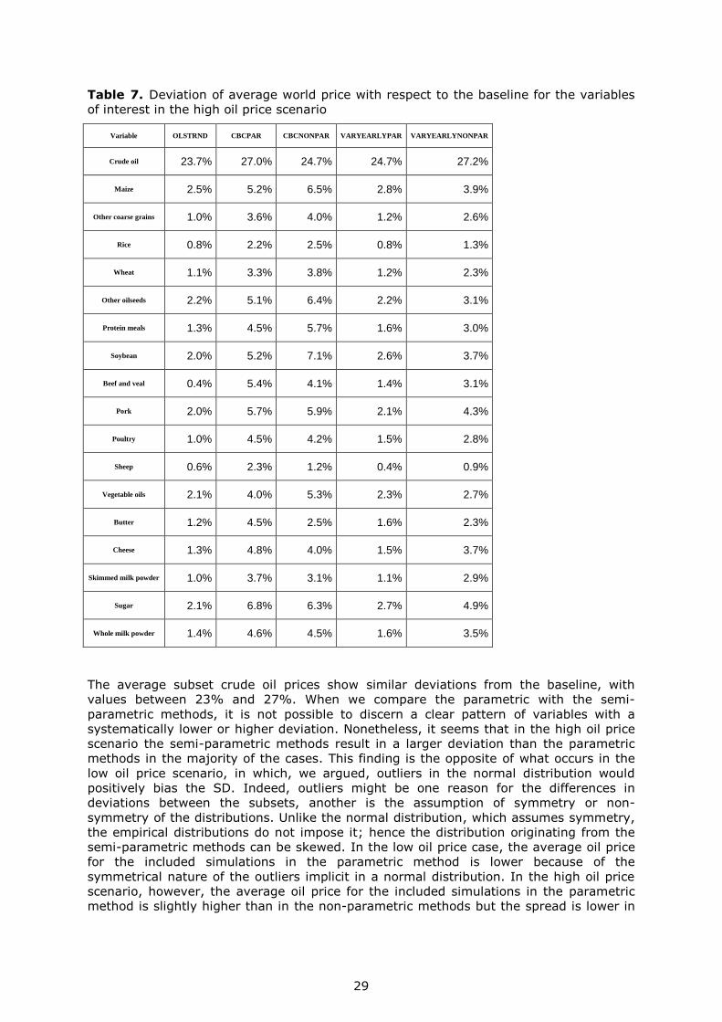
and these will bias the standard deviation by increasing it.
The results of the subset analysis for the high oil price scenario are shown in Table 7.
29
Table 7. Deviation of average world price with respect to the baseline for the variables
of interest in the high oil price scenario
Variable OLSTRND CBCPAR CBCNONPAR VARYEARLYPAR VARYEARLYNONPAR
Crude oil 23.7% 27.0% 24.7% 24.7% 27.2%
Maize 2.5% 5.2% 6.5% 2.8% 3.9%
Other coarse grains 1.0% 3.6% 4.0% 1.2% 2.6%
Rice 0.8% 2.2% 2.5% 0.8% 1.3%
Wheat 1.1% 3.3% 3.8% 1.2% 2.3%
Other oilseeds 2.2% 5.1% 6.4% 2.2% 3.1%
Protein meals 1.3% 4.5% 5.7% 1.6% 3.0%
Soybean 2.0% 5.2% 7.1% 2.6% 3.7%
Beef and veal 0.4% 5.4% 4.1% 1.4% 3.1%
Pork 2.0% 5.7% 5.9% 2.1% 4.3%
Poultry 1.0% 4.5% 4.2% 1.5% 2.8%
Sheep 0.6% 2.3% 1.2% 0.4% 0.9%
Vegetable oils 2.1% 4.0% 5.3% 2.3% 2.7%
Butter 1.2% 4.5% 2.5% 1.6% 2.3%
Cheese 1.3% 4.8% 4.0% 1.5% 3.7%
Skimmed milk powder 1.0% 3.7% 3.1% 1.1% 2.9%
Sugar 2.1% 6.8% 6.3% 2.7% 4.9%
Whole milk powder 1.4% 4.6% 4.5% 1.6% 3.5%
The average subset crude oil prices show similar deviations from the baseline, with
values between 23% and 27%. When we compare the parametric with the semi-
parametric methods, it is not possible to discern a clear pattern of variables with a
systematically lower or higher deviation. Nonetheless, it seems that in the high oil price
scenario the semi-parametric methods result in a larger deviation than the parametric
methods in the majority of the cases. This finding is the opposite of what occurs in the
low oil price scenario, in which, we argued, outliers in the normal distribution would
positively bias the SD. Indeed, outliers might be one reason for the differences in
deviations between the subsets, another is the assumption of symmetry or non-
symmetry of the distributions. Unlike the normal distribution, which assumes symmetry,
the empirical distributions do not impose it; hence the distribution originating from the
semi-parametric methods can be skewed. In the low oil price case, the average oil price
for the included simulations in the parametric method is lower because of the
symmetrical nature of the outliers implicit in a normal distribution. In the high oil price
scenario, however, the average oil price for the included simulations in the parametric
method is slightly higher than in the non-parametric methods but the spread is lower in

30
the latter (see Figure 3). This is due to the fact that different methods replicate different
ranges for the oil price uncertainty.
Overall we observe that the mean of the simulations is affected by the extraction
method, while the SD and its skewness are affected by the nature of the simulation
technique (parametric or semi-parametric). The SD and its skewness are more crucial
for the subset analysis because they are related to the shape of the distribution and the
position of the quantiles.
6.2 Yield uncertainty
So far we have argued that normality by means of symmetry and long tails of the
probabilistic distribution (i.e. allowing values at either extreme of the distribution, which
potentially create outliers) can bias the results, therefore, creating simulations that do
not fit the extracted data. Another implication of the simulated probabilistic distribution
is the correlation between yields in different regions. The correlation remains a key issue
when doing subset analysis for which the subsample is conditional on observations
meeting specific criteria (i.e. values below a threshold or within a range). For example,
we perform a scenario analysis with a subset sample in which wheat yields in Russia,
Ukraine and Kazakhstan are below the 50th percentile. Only the simulations in which the
wheat yield in those three countries are below the 50th percentile are included.
Moreover, we limit the analysis to the variables we consider to be most interesting for
this analysis: yield, production, producer prices, and exports.
First, following the example of the scenarios for macroeconomic variables, we report,
without sub-setting, descriptive statistics for the variables in each of the simulation
methods tested (Table 8).
Table 8. Main statistics for the variables of interest in the three yield uncertainty
methodologies
Country Variable
CBCNONPAR CBCPAR OLSTRND
Average SD CV Average SD CV Average SD CV
Kazakhstan
Exports 6 342 2 659 42% 6 226 2 821 45% 5 954 2 772 47%
Producer
price 63 183 6 667 11% 64 125 10 072 16% 68 583 9 840 14%
Production 15 077 2 994 20% 14 902 3 335 22% 14 558 3 260 22%
Yield 1.35 0.54 40% 1.34 0.57 42% 1.28 0.54 42%
Russia
Exports 32 680 6 301 19% 32 853 6 878 21% 32 025 4 942 15%
Producer
price 10 556 869 8% 10 582 1 208 11% 11 241 1 008 9%
Production 68 605 8 404 12% 68 879 9 366 14% 67 719 6 812 10%
Yield 2.5 0.55 22% 2.52 0.66 26% 2.34 0.43 19%
Ukraine
Exports 15 418 4 033 26% 15 503 4 710 30% 14 032 4 060 29%
Producer
price 3 103 291 9% 3 121 421 14% 3 362 446 13%

31
Country Variable
CBCNONPAR CBCPAR OLSTRND
Average SD CV Average SD CV Average SD CV
Production 29 493 4 425 15% 29 605 5 287 18% 27 969 4 506 16%
Yield 4.38 1.23 28% 4.46 1.52 34% 3.97 1.2 30%
World
Exports 181 800 5 828 3% 182 280 7 873 4% 178 795 5 709 3%
Production 806 070 16 086 2% 807 597 20 602 3% 802 931 16 193 2%
World
price 242 17 7% 242 24 10% 257 21 8%
The original method (OLSTRND) has the lowest average for all variables except prices.
Using the cubic trend extraction method, the parametric and semi-parametric simulation
methods result in different values. The way we simulate the uncertainty distributions in
the future seems more important than the uncertainty extraction methods. These
simulated uncertainty distributions have a recursive effect that does not necessarily
appear in the same year as the shock. Most of the yield shock is transmitted to the
following year by its effect as an exogenous (shocked) variable in the returns per
hectare equation. Thus, the distribution of final simulated yields has a long-lasting effect
on the variables resulting from the model analysed here. With regard to the SD, the
cubic polynomial with a parametric distribution (CBCPAR) has the largest absolute values
for each variable. Nonetheless, in relative terms to the mean (i.e. in terms of the
coefficient of variation), such a pattern is less clear.
The number of simulations fulfilling the selection criteria differs in each of the
methodologies. For the OLSTRND, CBCNONPAR and CBCPAR methodologies, the number
of simulations is 190, 449 and 200, respectively. Note that the two parametric methods
have a similar subset size, whereas in the semi-parametric method the number of
simulations fulfilling the criteria is more than doubled. This is the outcome of the Clayton
copula whereby we have assumed low tail dependence and, therefore, the correlation
among simulations with below-average yield is strong (see Figure 5).

32
Figure 5. Scatterplot for wheat yield uncertainty in Ukraine and Russia, cubic-parametric and
semi-parametric methods indicating subsets
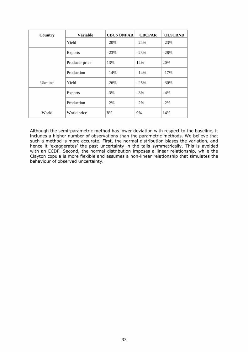
Next, we analyse the yield deviation from the baseline for each method. The values are
similar for both parametric methods, OLSTRND and CBCPAR, while in the CBCNONPAR
method the deviation is lower (Table 9). The results are consistent with our previous
findings. The normal distribution creates extreme cases that bias the variation (see
Figure 1 dispersion, where the parametric method produces extreme cases not observed
in the ECDF–Clayton copula). Following the larger deviation of the yield for the
parametric methods, the rest of the variables also have larger deviation than in the
semi-parametric method, almost in all cases.
Table 9. Deviation of the yield scenario with respect to the baseline for the variables of
interest
Country Variable CBCNONPAR CBCPAR OLSTRND
Kazakhstan
Exports –33% –37% –40%
Producer price 16% 19% 25%
Production –17% –20% –21%
Yield –29% –33% –35%
Russia
Exports –15% –19% –16%
Producer price 10% 12% 16%
Production –11% –13% –12%
33
Country Variable CBCNONPAR CBCPAR OLSTRND
Yield –20% –24% –23%
Ukraine
Exports –23% –23% –28%
Producer price 13% 14% 20%
Production –14% –14% –17%
Yield –26% –25% –30%
World
Exports –3% –3% –4%
Production –2% –2% –2%
World price 8% 9% 14%
Although the semi-parametric method has lower deviation with respect to the baseline, it
includes a higher number of observations than the parametric methods. We believe that
such a method is more accurate. First, the normal distribution biases the variation, and
hence it ‘exaggerates’ the past uncertainty in the tails symmetrically. This is avoided
with an ECDF. Second, the normal distribution imposes a linear relationship, while the
Clayton copula is more flexible and assumes a non-linear relationship that simulates the
behaviour of observed uncertainty.
34
7 Implications of the proposed methodologies
The implementation of new methodologies for the PSA with Aglink-Cosimo poses some
challenges that have already been acknowledged. The first and most important is the
limited number of observations in the past from which to extract the uncertainty. There
are fewer observations available for macroeconomic variables than for yield variables. In
the methodologies proposed for macroeconomic uncertainty we deal with this issue by
performing VARs including variables for each country considered. For the extraction of
the past yield uncertainty, the cubic polynomial offers reasonable results and the current
number of observations allows the estimation. Nonetheless, as the number of historical
observations remains low, new data incorporated in the analysis can potentially shift the
results, especially if they come from a harvest failure or a bumper crop year.
Among the proposed methods, we tested the use of parametric and semi-parametric
methods. The latter do not impose a distribution on the marginal distributions, which we
think is less restrictive and, thus, preferable. The parametric methods have been shown
to bias the variance of the true distributions, hence yielding outliers in the simulations,
especially in the distribution tails. By distributing the uncertainty equally, such methods
do not accurately replicate the past uncertainty. Indeed, the KCD tests confirmed our
hypothesis, as the results for the parametric simulation method reject the null
hypothesis of this test. This finding therefore confirms that the extracted uncertainty
does not follow a normal distribution for any of the extraction methods. Thus, for
simulations, it is best to make use of the empirical distributions rather than imposing a
functional form that can bias the simulations.
Additionally, looking at the bias of the variance, the normal distribution assumes a linear
relationship among the variables. On the other hand, the copula method corrects this
issue by assuming non-linearity with tail dependence. We think that this more flexible
system is better. In this sense, it would be interesting to carry out further research to
determine the true nature of the correlations among actual variables, potentially with
bootstrapping procedures as described in Genest et al. (2009).
Overall, despite having lower variation, the semi-parametric methods should be
preferred over their parametric counterparts. The simulated uncertainty represents, in
this case, more closely the true distribution of the measured uncertainty. For a
stochastic method considering the yield variables, our recommendation is to use the
cubic trend for extracting the uncertainty and the Clayton copula with ECDF marginal
distributions for simulating the uncertainty. For a stochastic method considering the
macroeconomic indicators, we recommend the use of a VAR for extracting the
uncertainty and a Frank copula with ECDF marginal distributions for simulating the
uncertainty.
The methods presented are just a few of the many options that could be implemented.
More flexible methods, such as Vine copulas, could provide further insights into the yield
uncertainty but are more complex and data demanding. The methodologies we propose
in this report are well documented in the literature, easy to implement, and require
fewer data than other methods.
The semi-parametric methods are more flexible than the parametric ones, which impose
a certain functional form. For this reason, they are also more prone to changes if
observations are added to the historical data, especially if the data come from extreme
cases. This behaviour should be reflected in our simulations in as much as it reflects the
fact that uncertainty has a changing nature.
Finally, the uncertainty considered in the PSA is based on past observations. We
acknowledge that in the future we might have new sources of variability (e.g. climate
change). Nonetheless, our aim is not to speculate on unobserved future sources of
uncertainty, but rather to provide a benchmark for policy, technical and scientific
analysis, based on plausible assumptions on past observed variability.
35
8 References
Araujo-Enciso, S., Fellmann, T., Pérez Domínguez, I. and Santini, F. (2016). ‘Abolishing
biofuel policies: possible impacts on agricultural price levels, price variability and global
food security’. Food Policy, Vol. 61(C), pp. 9-26.
Araujo-Enciso, S., Pérez Domínguez, I., Santini, F. and Helaine, S. (2015).
Documentation of the European Commission’s EU module of the Aglink-Cosimo modelling
system. EUR 27138, Scientific and Technical Reports — Institute for Prospective
Technological Studies.
Burrell, A. and Nii-Naate, Z. (2013). Partial stochastic analysis with the European
Commission’s version of the AGLINK-COSIMO model. EUR 2589, Reference Reports —
Joint Research Centre Institute for Prospective Technological Studies.
European Commission (2016). Medium-term prospects for EU agricultural markets and
income 2016-2026. Brussels
Genest, C., Rémillard, B. and Beaudoin, D. (2009). ‘Goodness-of-fit tests for copulas: a
review and a power study’.” Insurance: Mathematics and Economics, Vol. 44, Issue 2,
pp. 199-213.
Goodwin, B. and Hungerford, A. (2015). “Copula-based models of systemic risk in U.S.
agriculture: implications for crop insurance and reinsurance contracts.” American Journal
of Agricultural Economics, Vol. 97, Issue 3, pp. 879-896.
Goodwin, B.K. and Ker, A.P. (1998). ‘Non parametric estimation of crop yield
distributions: implications for rating group-risk crop insurance contracts.” American
Journal of Agricultural Economics, Vol. 80, Issue 1, pp. 139-153.
Goodwin, B.K. and Mahul, O. (2004). ‘Risk modeling concepts relating to the design and
rating of agricultural insurance contracts’. World Bank Publications, 37 pages.
Hayfield, T. and Racine, J.S. (2008). ‘Nonparametric econometrics: the np package’.
Journal of Statistical Software, Vol. 27, Issue 5. URL: http://www.jstatsoft.org/v27/i05/.
Ker, A.P. and Goodwin, B.K. (2000). ‘Non parametric estimation of crop insurance rates
revisited’. American Journal of Agricultural Economics, Vol. 82, Issue 2, pp. 463-478.
Li Q., Maasoumi E. and Racine, J.S. (2009). ‘A nonparametric test for equality of
distributions with mixed categorical and continuous data’. Journal of Econometrics, Vol.
148, pp. 186-200.
Lütkepohl, H. (2004). Vector Autoregressive and Vector Error Correction Models. In
Applied Time Series Econometrics. Lütkepohl, H. and Krätzig, M. (eds), pp 86-158
Okhrin, O. and Ristig, A. (2014). ‘Hierarchical Archimedean Copulae: the HAC package’.
Journal of Statistical Software, Vol. 58, Issue 4.
Ramirez, O.A., Misra, S. and Field, J. (2003). ‘Crop-yield distributions revisited’ American
Journal of Agricultural Economics, Vol. 85, Issue 1, pp. 108-120.
Sherrick, B.J., Zanini, F.C., Schnitkey, G.D. and Irwin, S.H. (2004). ‘Crop insurance
valuation under alternative yield distributions’. American Journal of Agricultural
Economics, Vol. 86, Issue 2, pp. 406-419.

36
doi:10.2791/843461
ISBN 978-92-79-59362-8
doi:10.2760/680976
ISBN: 978-92-79-76018-1
KJ-N
A-2
8863-E
N-N