Embed Size (px)
Citation preview

Partial Parallel Interference Cancellation
Based on Hebb Learning Rule
Taiyuan University of Technology
Yanping Li

Content
Background Hebb Learning Rule CDMA System Model PIC PPIC Hebb-PPIC Simulations and Conclusion References

Background (1)
Multiuser Detection– In CDMA systems MAI (Multiple-access Interferen
ce) will be the main factor of damaging system performance when the number of users is relatively large. The methods of rejecting MAI mainly include improving the design of spreading code, power control, space filtering and multiuser detection [1, 2].
– Multiuser detection applies the correlation between the expected user and interference users to MAI cancellation.

Background (2)
Parallel Interference Cancellation (PIC)– PIC is one of nonlinear multiuser detection approa
ches, and it can obtain obvious performance improvement at the cost of low computing complexity and short processing delay.
– The PIC process is shown in the next page.
Background (3)
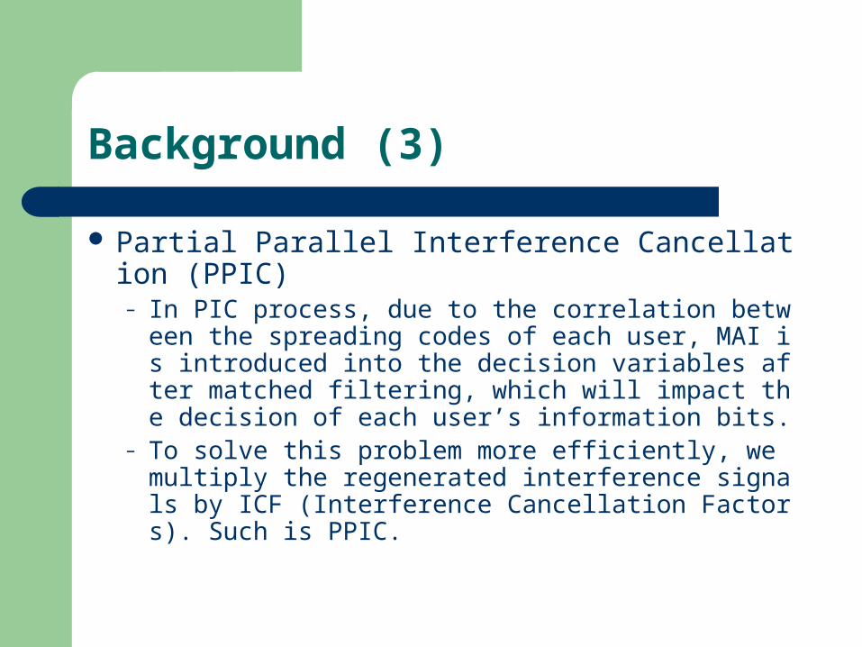
Partial Parallel Interference Cancellation (PPIC)– In PIC process, due to the correlation between th
e spreading codes of each user, MAI is introduced into the decision variables after matched filtering, which will impact the decision of each user’s information bits.
– To solve this problem more efficiently, we multiply the regenerated interference signals by ICF (Interference Cancellation Factors). Such is PPIC.

Hebb Learning Rule (1)
Hebb Learning Rule– Hebb learning rule is one of the neural network le
arning rules widely used. It was proposed by Donald Hebb in 1949 as a potential mechanism for the brain to adjust its neuron synapse and from then on it has been used in training artificial neural network [3].
– Hebb learning rule is based on Hebb assumption.

Hebb Learning Rule (2)
Hebb Assumption [4]– When an axon of cell A is near enough to excite a
cell B and repeatedly or persistently takes part in firing it, some growth process or metabolic change takes place in one or both cells such that A’s efficiency, as one of the cells firing B, is increased.
– Hebb assumption means that if a positive input results in a positive output , should be increased.
jp
ia ijw

Hebb Learning Rule (3)
– Such is a kind of mathematics explanation for it:
– also simplified as
– where is the jth element of the qth input vector , is the ith element of network output when the qth input vector is entered into the network and is a positive constant called as learning rate.
( ) ( )new oldij ij i iq j jqw w f a g p
new oldij ij iq jqw w a p
jqp
qp iqa

Hebb Learning Rule (4)
– It should be noticed that Hebb assumption can be expanded as follows: the variation of weights is proportional to the product of active values from each side of synapse. Therefore, weights will increase not only when and are both positive but also when they are both negative. Besides, Hebb rule will decrease weights as long as and have opposite signs.
jp ia
jp ia

CDMA System Model (1)
Synchronous DS-CDMA System Model– Consider a DS-CDMA system where K users
transmit their information synchronously over a common additive white Gaussian noise (AWGN) channel. The received signal at the base station can be modeled as [5]
1
( ) ( ) ( )K
j j jj
i A b i i
r s n

CDMA System Model (2)
– where– is received amplitude of the jth user, – is transmitted symbol (±1) of the jth user,– is signature vector of the jth user,– and is an AWGN vector.
jA
jb i
js
( )in

CDMA System Model (3)
MC-CDMA System Model– In a MC-CDMA system where K users transmit th
eir information synchronously over a common AWGN channel, the received nth chip of the ith bit at the base station can be described in discrete-time form
1
, ,1 0
( ) ( ) ( ) ( )K N
i j i j i ij l
y n h l s n l z n
CDMA System Model (4)
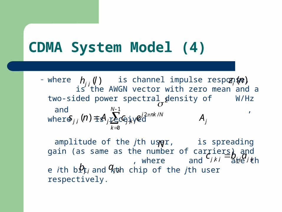
– where is channel impulse response, is the AWGN vector with zero mean and a two-sided power spectral density of W/Hz
and , where is received
amplitude of the jth user, is spreading gain (as same as the number of carriers) and , where and are the ith bit and kth chip of the jth user respectively.
, ( )j ih l ( )iz n
21
2 /, , ,
0
( )N
j nk Nj i j j k i
k
s n A c e
jA
N
, , , ,j k i j i j kc b a,j ib ,j ka

PIC (1)
– The decision variable at stage 1 (output of MF (Matched Filter)) in conventional PIC is [5]
– where is the correlation coefficient between spreading codes of the ith user and kth user.
– The output after decision is
(1)
1,
,K
i i i ik k k ik k i
r Ab A b n
1, ,i K
ik
(1) (1)ˆ sgn[ ],i ib r 1, ,i K

PIC (2)
– The decision variables of the following stages (interference cancellation stages) are
– and the corresponding decision outputs are
( ) ( 1)
1,
ˆ( ) ,K
m mi i i ik k k k i
k k i
r Ab A b b n
1, , ,i K 2,3, ,m
( ) ( )ˆ sgn[ ],m mi ib r 1, , .i K

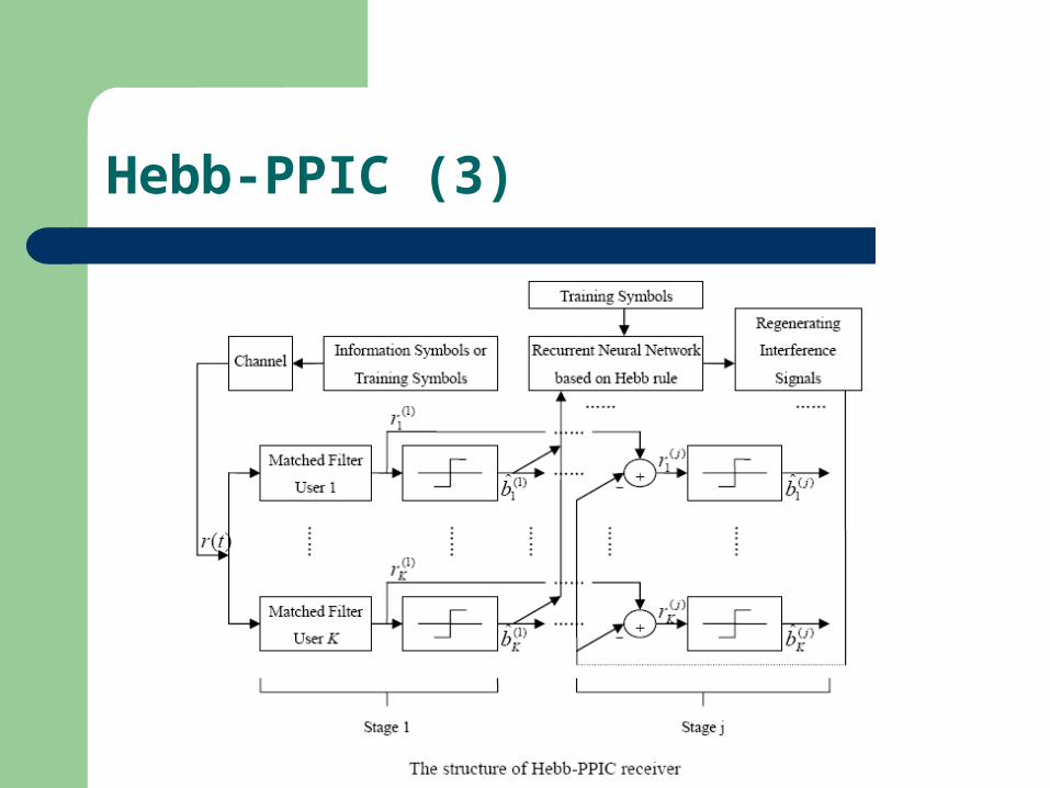
PIC (3)

PPIC (1)
– The decision variables at interference cancellation stages in PPIC with ICF are
– where is the ICF of the ith user at stage m.
( ) ( ) ( 1)
1,
ˆ( ) ,K
m m mi i i ik k k i k i
k k i
r Ab A b w b n
1, , ,i K 2,3, ,m
( )miw

PPIC (2)

Hebb-PPIC (1)
– Apply recurrent neural network based on Hebb learning rule to adjusting :
– where , is the learning rate and saturated linear function satlin is used to assure the convergence of learning process.
( ) ( 1) ( 1) ( 1)ˆ{ [1 (1 )]},m m m mi i i iw satlin w b b
1, , ,i K 2,3, ,m
( )miw
(1) 1, 1, ,iw i K (0,1)

Hebb-PPIC (2)
Hebb-PPIC (3)
Simulations and Conclusion (1)
Based on the analysis above several computer simulations are presented in the conditions of ideal power control and “near-far” scenario to compare the performance of Hebb-PPIC with that of PIC or MF (namely DEC (decorrelation) in MC-CDMA system) detection.

Simulations and Conclusion (2)
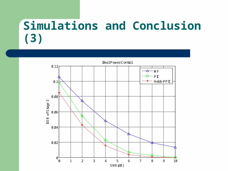
Ideal Power Control– Simulation 1 (in DS-CDMA system) :– number of users K = 5 ; number of stages m=5; n
oise power spectral density ; the processing gain N = 32 ;number of test bits ; . The BER curves of MF detector, PIC and Hebb-PPIC detectors (at stage 3) versus SNR are given below:
2 1
1000bN 1/ 20
Simulations and Conclusion (3)
0 1 2 3 4 5 6 7 8 9 100
0.02
0.04
0.06
0.08
0.1
0.12Ideal Power Control
SNR(dB)
BE
R o
f S
tage
3
MF
PICHebb-PPIC

Simulations and Conclusion (4)
– From this figure we can see that the BER decreases all along with increasing of SNR and moreover, the BER curve of Hebb-PPIC is under those of MF and PIC all the time. Especially when SNR is low (not exceeding 4dB), the BER of Hebb-PPIC is 1 to 2 percentage points lower than MF and 0.5 to 1 percentage points than PIC in [5], which indicates that Hebb-PPIC performs better in noisy communication environment.

Simulations and Conclusion (5)
– Simulation 2 (in MC-CDMA system) : – amplitude of users ; m=5; ;
N = 32 ; ; . The BER curves of PIC and Hebb-PPIC detectors versus stage are shown in the next figure.
1, 1, ,iA i K 2 1 1000bN 1/ 200

Simulations and Conclusion (6)
1 1.5 2 2.5 3 3.5 4 4.5 50
0.005
0.01
0.015
0.02
0.025
0.03Ideal Power Control
Stage
BE
R
PIC
Hebb-PPIC

Simulations and Conclusion (7)
– From the figure above we can find that the BERs of both PIC and Hebb-PPIC decrease along with stage and especially from stage 1 to stage 2 they decrease very obviously and tend to be stable from stage 2 on. On the other hand, the BER curve of Hebb-PPIC is under that of PIC all the while from stage 1 to stage 5, which indicates that on the basis of PIC structure Hebb-PPIC improves the reception performance of system further, i.e., weakens the effect resulted from error cancellation in PIC.

Simulations and Conclusion (8)
“Near-Far” Scenario– Simulation 3 (in DS-CDMA system) :– K=10; , and denote amplitude of
the strong users and weak users respectively; m=5; ; N=32; ; . BER curves of weak user group and strong user group versus SNR are presented as follows:
2 1 1000bN 1/ 20
/ 5s wA A db sA wA

Simulations and Conclusion (9)
0 1 2 3 4 5 6 7 8 9 100
0.02
0.04
0.06
0.08
0.1
0.12
0.14
0.16
0.18Near-Far Scenario
SNR(dB)
BE
R o
f th
e w
eak
user
gro
up a
t st
age
3
PIC
Hebb-PPIC

Simulations and Conclusion (10)
0 1 2 3 4 5 6 7 8 9 100
0.02
0.04
0.06
0.08
0.1
0.12
0.14Near-Far Scenario
SNR(dB)
BE
R o
f th
e st
rong
use
r gr
oup
at s
tage
3
PIC
Hebb-PPIC
Simulations and Conclusion (11)
– From the two figures we observe that the BER of Hebb-PPIC and PIC is decreasing all the time when SNR is increasing and the corresponding curves of Hebb-PPIC is under those of PIC in [5] all along for both user groups. Especially for weak users the BER of Hebb-PPIC is 4 to 6 percentage points lower than PIC while it is 0.5 to 2 percentage points for strong users, which shows that Hebb-PPIC detection can be able to reject “near-far” effect more efficiently.

Simulations and Conclusion (12)
– Simulation 4 (in MC-CDMA system) :– K=10; , and denote amplitude of
the strong users and weak users respectively; m=5; ; N=32; ; . BER curves of weak user group and strong user group versus SNR are presented as follows:
2 1 1000bN 1/50
/ 5s wA A db sA wA
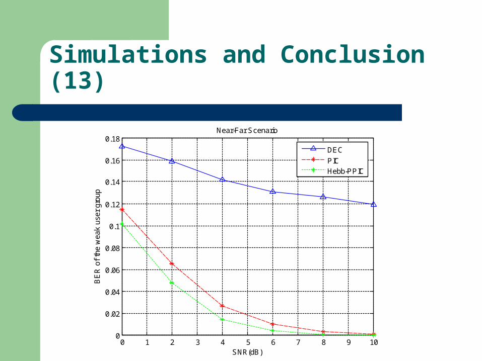
Simulations and Conclusion (13)
0 1 2 3 4 5 6 7 8 9 100
0.02
0.04
0.06
0.08
0.1
0.12
0.14
0.16
0.18Near-Far Scenario
SNR(dB)
BE
R o
f th
e w
eak
user
gro
up
DEC
PICHebb-PPIC

Simulations and Conclusion (14)
– In this figure it can be easily seen that for weak users the BER level of PIC and Hebb-PPIC is far lower than that of DEC and even with the biggest SNR (10 dB) the BER of DEC (12%) is higher than that of PIC and Hebb-PPIC (about 11.5%) with the smallest SNR (0 dB). Although becoming nearer to the BER curve of PIC along with increasing of SNR, that of Hebb-PPIC is still under it.

Simulations and Conclusion (15)
0 1 2 3 4 5 6 7 8 9 100
0.02
0.04
0.06
0.08
0.1
0.12
0.14Near-Far Scenario
SNR(dB)
BE
R o
f th
e st
rong
use
r gr
oup
DEC
PICHebb-PPIC
Simulations and Conclusion (16)
– From this figure we notice that compared with weak user group the distances between the three BER curves are not too large in the case of strong user group, and when SNR is relatively small (0~2 dB) the BER of DEC is even lower than that of PIC, which is because that small SNR means serious interference while this will result in error decision and cancellation which will influence the veracity of decisions at the next stage. But with SNR increasing (bigger than 2 dB), the advantage of PIC will emerge that its BER is 1 to 2 percentage points lower than DEC’s.

Simulations and Conclusion (17)
– Comparing these two figures we can find that when the user signals are weak PIC, especially Hebb-PPIC, will play an important role in improving reception performance and rejecting “near-far” effects.
Simulations and Conclusion (18)
The Hebb-PPIC algorithm is simulated in two conditions of idea power control and “near-far” scenario. Simulation results indicate that no matter which parameter changes among stage number, SNR and number of active users, the BER performance of Hebb-PPIC is generally better than conventional PIC.

Simulations and Conclusion (19)
On the other hand, compared with most of the PPIC algorithms proposed by now, Hebb-PPIC has the advantage of small computing quantity, low complexity and easy implementation and it can adjust ICF at any moment of channel variation, so it owns practicability in engineering.

References
[1] S. Verdu, “Minimum probability of error for asynchronous Gaussian multiple-access channels,” IEEE Trans. Inf. Theory, vol. 32, no. 1, pp. 85-96, Jan. 1986.
[2] R. Lupas, and S. Verdu, “Linear multiuser detectors for synchronous code-division multiple-access channels,” IEEE Trans. Inf. Theory, vol. 35, no. 1, pp. 123-135, Jan. 1989.
[3] M. T. Hagan, H. B. Demuth, and M. H. Beale, Neural Network Design, Beijing: China Machine Press, 2002.
[4] D. O. Hebb, The Organization of Behavior, Massachusetts: MIT Press, 2000.
[5] G. B. Giannakis, Y. Hua, and P. Stoica, Signal Processing Advances in Wireless and Mobile Communications, Beijing: Posts & Telecommunications Press, 2002.

Thank you!