Embed Size (px)
Citation preview
Simple Neural Nets for Pattern Classification Hebb Nets, Perceptrons and Adaline Nets
Based on Fausette’s Fundamentals of Neural Networks
McCulloch-Pitts networks
• In the previous lecture, we discussed Threshold Logic and McCulloch-Pitts networks based on Threshold Logic.
• McCulloch-Pitts networks can be use do build networks that can compute any logical function.
• They can also simulate any finite automaton (although we didn’t discuss this in class).
• Although the idea of thresholds and simple computing units are biologically inspired, the networks we can build are not very relevant from a biological perspective in the sense that they are not able to solve any interesting biological problems.
• The computing units are too similar to conventional logic gates and the networks must be completely specified before they are used.
• There are no free parameters that can be adjusted to solve different problems.
McCulloch-Pitts Networks
• Learning can be implemented in McCulloch-Pitts networks by changing the connections and thresholds of units.
• Changing connections or thresholds is normally more difficult that adjusting a few numerical parameters, corresponding to connection weights.
• In this lecture, we focus on networks with weights on the connections. • Learning will take place by changing these weights. • In this chapter, we will look at a few simple/early networks types
proposed for learning weights. • These are single-layer networks and each one uses it own learning rule. • The network types we look at are: Hebb networks, Perceptrons and
Adaline networks.
Learning Process/Algorithm
• In the context of artificial neural networks, a learning algorithm is an adaptive method where a network of computing units self-organizes by changing connections weights to implement a desired behavior.
• Learning takes place when an initial network is “shown” a set of examples that show the desired input-output mapping or behavior that is to be learned. This is the training set.
• As each example is shown to the network, a learning algorithm performs a corrective step to change weights so that the network slowly “learns” to produce the desired response.
Learning Process/Algorithm
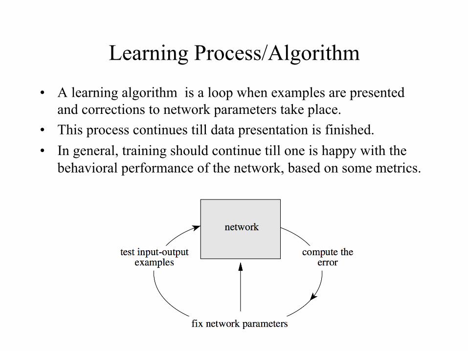
• A learning algorithm is a loop when examples are presented and corrections to network parameters take place.
• This process continues till data presentation is finished. • In general, training should continue till one is happy with the
behavioral performance of the network, based on some metrics.
Classes of Learning Algorithms
• There are two types of learning algorithms: supervised and unsupervised.
• Supervised Learning: – In supervised learning, a set of “labeled” examples is shown to the
learning system/network. – A labeled example is a vector with “features” of the training data
sample along with the “correct” answer given by a “teacher”. – For each example, the system computes the deviation of the output
produced by the network with the correct output and changes/corrects the weights according to the magnitude of the error, as defined by the learning algorithm.
– Classification is an example of supervised learning.
Classes of Learning Algorithms
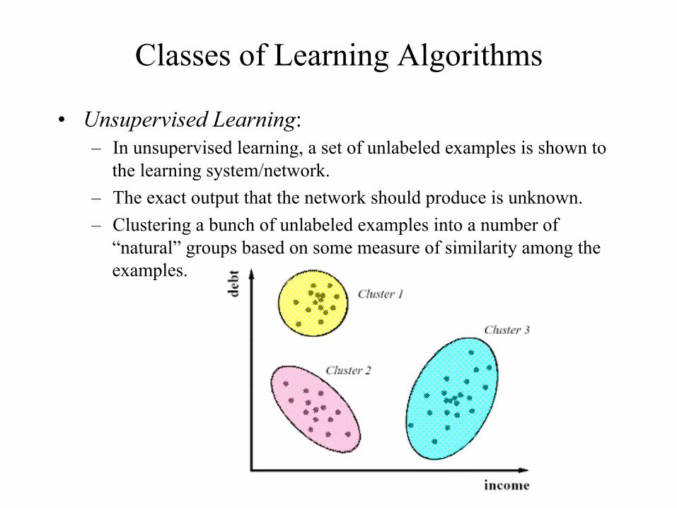
• Unsupervised Learning: – In unsupervised learning, a set of unlabeled examples is shown to
the learning system/network. – The exact output that the network should produce is unknown. – Clustering a bunch of unlabeled examples into a number of
“natural” groups based on some measure of similarity among the examples.
Classification • Patterns or examples to be classified are represented as a
vector of features (encoded as integers or real numbers in NN)
• Pattern classification: • Classify a pattern to one of the given classes • It is a kind of supervised learning
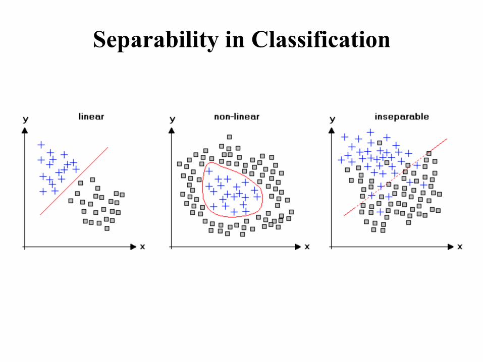
Separability in Classification
• Separability of data points is a very important concept in the context of classification.
• Assume we have data points with two dimensions or “features”.
• Data classes are linearly separable if we can draw a straight line or a (hyper-)plane separating the various classes.
Separability in Classification
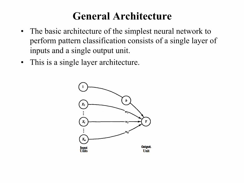
General Architecture • The basic architecture of the simplest neural network to
perform pattern classification consists of a single layer of inputs and a single output unit.
• This is a single layer architecture.
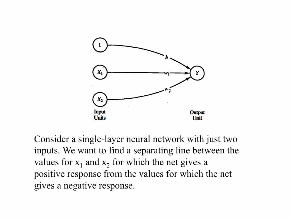
Consider a single-layer neural network with just two inputs. We want to find a separating line between the values for x1 and x2 for which the net gives a positive response from the values for which the net gives a negative response.
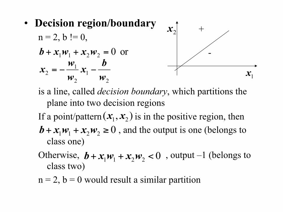
• Decision region/boundary n = 2, b != 0, is a line, called decision boundary, which partitions the
plane into two decision regions If a point/pattern is in the positive region, then
, and the output is one (belongs to class one)
Otherwise, , output –1 (belongs to class two)
n = 2, b = 0 would result a similar partition
21
2
12
2211 or 0
wbx
wwx
wxwxb
−−=
=++
2x
1x
+
-
),( 21 xx02211 ≥++ wxwxb
02211 <++ wxwxb
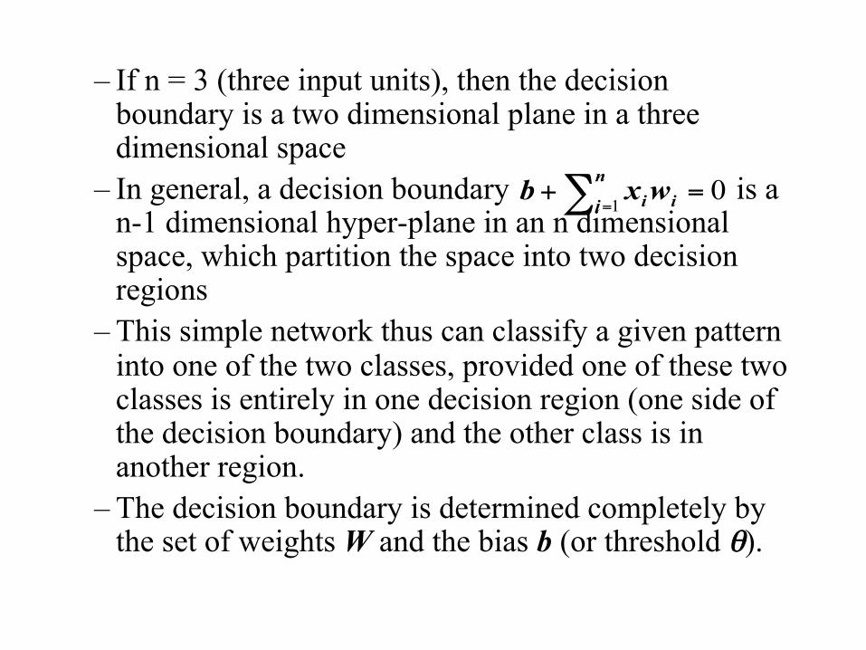
– If n = 3 (three input units), then the decision boundary is a two dimensional plane in a three dimensional space
– In general, a decision boundary is a n-1 dimensional hyper-plane in an n dimensional space, which partition the space into two decision regions
– This simple network thus can classify a given pattern into one of the two classes, provided one of these two classes is entirely in one decision region (one side of the decision boundary) and the other class is in another region.
– The decision boundary is determined completely by the set of weights W and the bias b (or threshold θ).
01
=+∑ =
n
i iiwxb
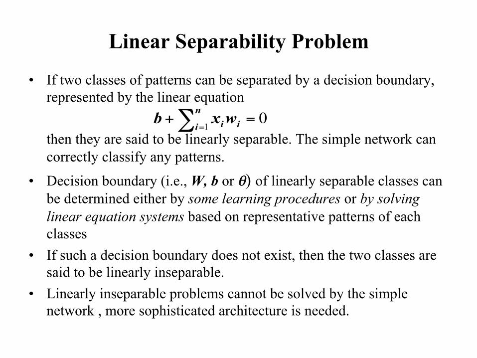
Linear Separability Problem
• If two classes of patterns can be separated by a decision boundary, represented by the linear equation
then they are said to be linearly separable. The simple network can correctly classify any patterns.
• Decision boundary (i.e., W, b or θ) of linearly separable classes can be determined either by some learning procedures or by solving linear equation systems based on representative patterns of each classes
• If such a decision boundary does not exist, then the two classes are said to be linearly inseparable.
• Linearly inseparable problems cannot be solved by the simple network , more sophisticated architecture is needed.
01
=+∑ =
n
i iiwxb
Linear Separability Problem
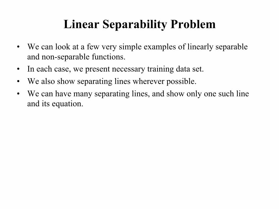
• We can look at a few very simple examples of linearly separable and non-separable functions.
• In each case, we present necessary training data set. • We also show separating lines wherever possible. • We can have many separating lines, and show only one such line
and its equation.
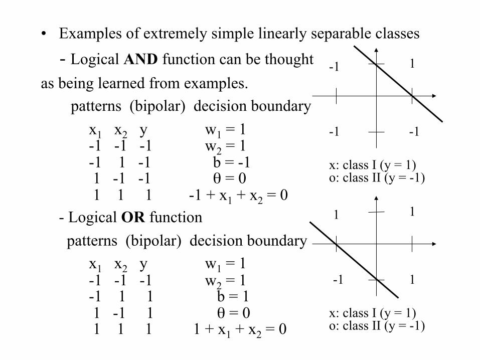
• Examples of extremely simple linearly separable classes - Logical AND function can be thought as being learned from examples.
patterns (bipolar) decision boundary x1 x2 y w1 = 1
-1 -1 -1 w2 = 1 -1 1 -1 b = -1
1 -1 -1 θ = 0 1 1 1 -1 + x1 + x2 = 0 - Logical OR function patterns (bipolar) decision boundary
x1 x2 y w1 = 1 -1 -1 -1 w2 = 1
-1 1 1 b = 1 1 -1 1 θ = 0 1 1 1 1 + x1 + x2 = 0
1
-1 -1
-1
x: class I (y = 1) o: class II (y = -1)
1
1 -1
1
x: class I (y = 1) o: class II (y = -1)
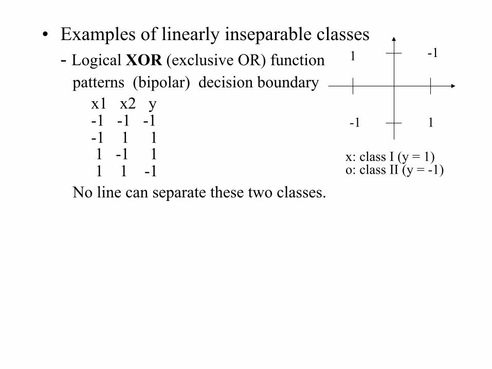
• Examples of linearly inseparable classes - Logical XOR (exclusive OR) function patterns (bipolar) decision boundary
x1 x2 y -1 -1 -1
-1 1 1 1 -1 1 1 1 -1 No line can separate these two classes.
-1
1 -1
1
x: class I (y = 1) o: class II (y = -1)
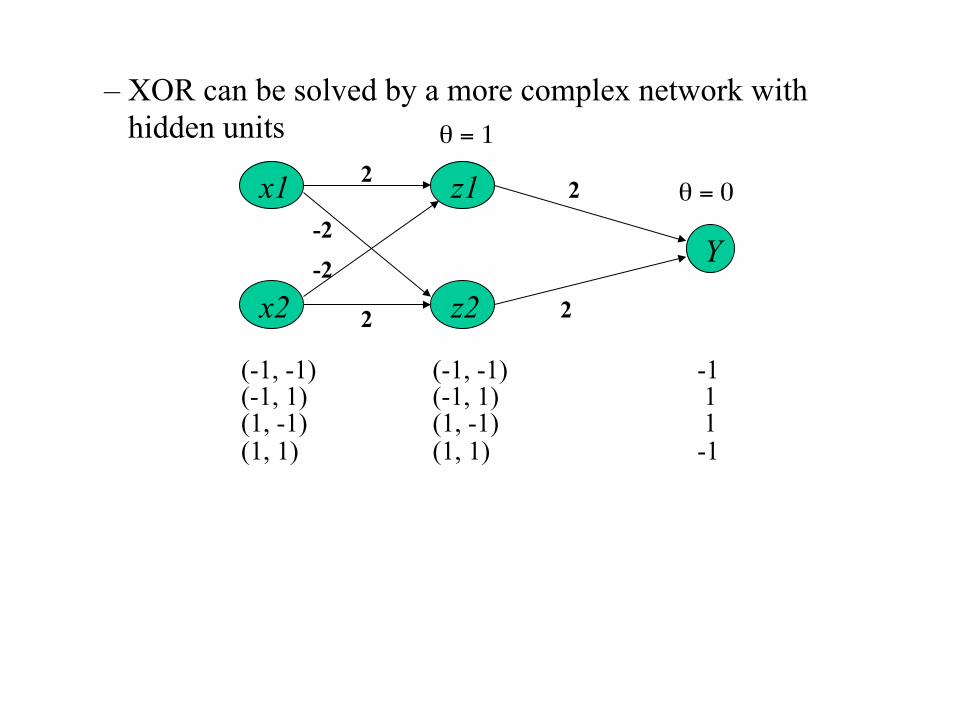
– XOR can be solved by a more complex network with hidden units
Y
z2
z1 x1
x2
2
2
2
2
-2
-2
θ = 1
θ = 0
(-1, -1) (-1, -1) -1 (-1, 1) (-1, 1) 1 (1, -1) (1, -1) 1 (1, 1) (1, 1) -1
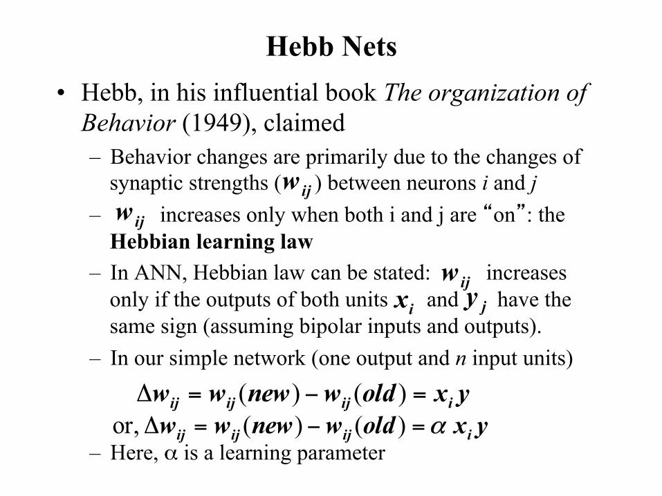
Hebb Nets • Hebb, in his influential book The organization of
Behavior (1949), claimed – Behavior changes are primarily due to the changes of
synaptic strengths ( ) between neurons i and j – increases only when both i and j are “on”: the
Hebbian learning law – In ANN, Hebbian law can be stated: increases
only if the outputs of both units and have the same sign (assuming bipolar inputs and outputs).
– In our simple network (one output and n input units)
– Here, α is a learning parameter
ijwijw
ijwix jy
yxoldwnewww iijijij =−=Δ )()(yxoldwnewww iijijij )()( or, α=−=Δ
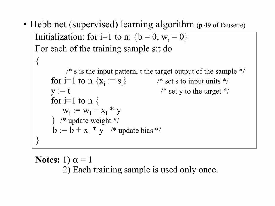
• Hebb net (supervised) learning algorithm (p.49 of Fausette)
Initialization: for i=1 to n: {b = 0, wi = 0} For each of the training sample s:t do {
/* s is the input pattern, t the target output of the sample */ for i=1 to n {xi := si} /* set s to input units */ y := t /* set y to the target */ for i=1 to n { wi := wi + xi * y
} /* update weight */ b := b + xi * y /* update bias */
} Notes: 1) α = 1 2) Each training sample is used only once.
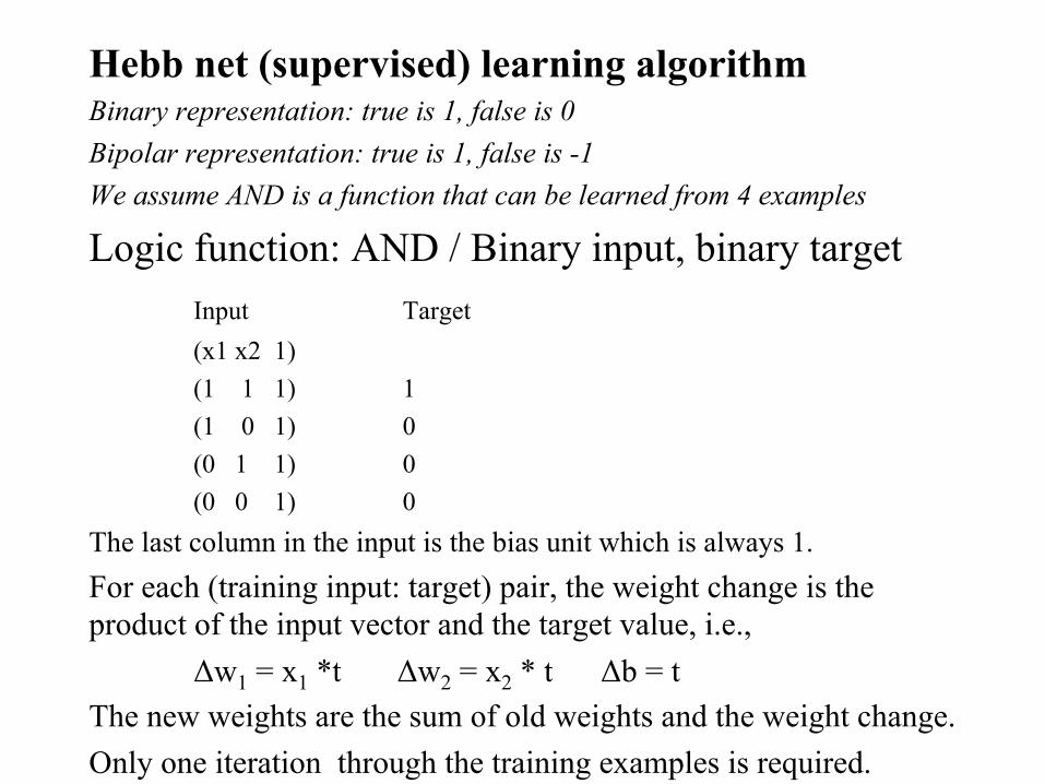
Hebb net (supervised) learning algorithm Binary representation: true is 1, false is 0 Bipolar representation: true is 1, false is -1 We assume AND is a function that can be learned from 4 examples
Logic function: AND / Binary input, binary target Input Target
(x1 x2 1) (1 1 1) 1 (1 0 1) 0
(0 1 1) 0 (0 0 1) 0 The last column in the input is the bias unit which is always 1. For each (training input: target) pair, the weight change is the product of the input vector and the target value, i.e.,
Δw1 = x1 *t Δw2 = x2 * t Δb = t The new weights are the sum of old weights and the weight change. Only one iteration through the training examples is required.
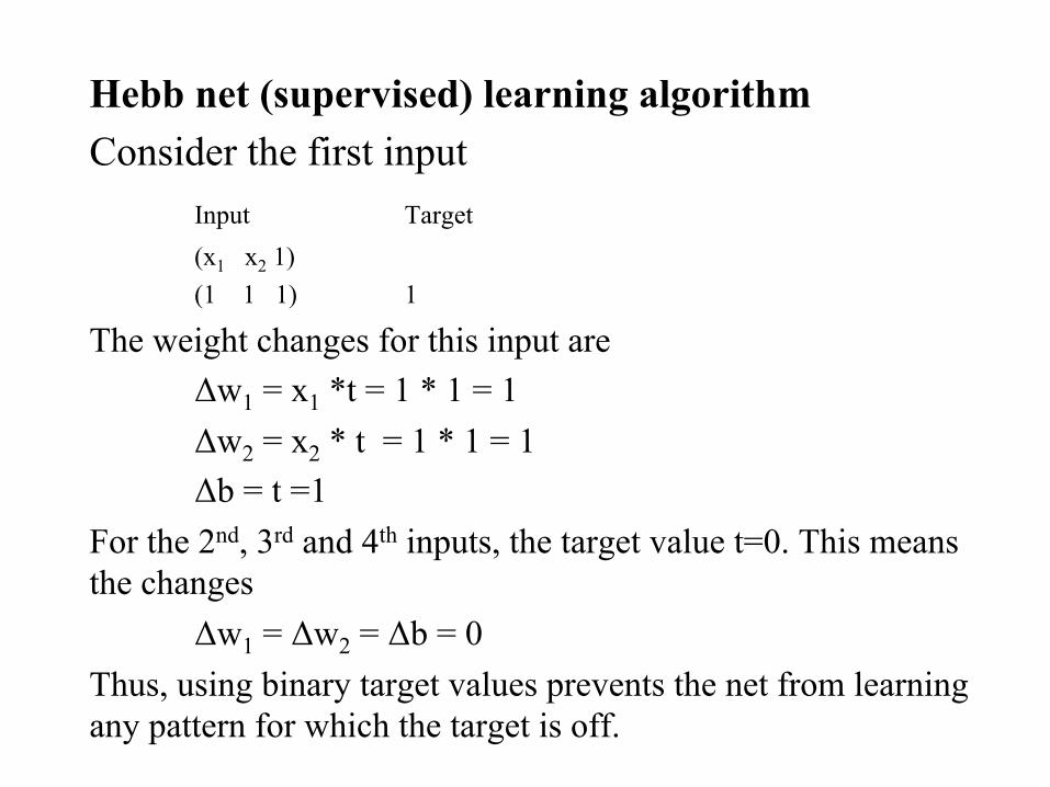
Hebb net (supervised) learning algorithm Consider the first input Input Target
(x1 x2 1) (1 1 1) 1
The weight changes for this input are Δw1 = x1 *t = 1 * 1 = 1 Δw2 = x2 * t = 1 * 1 = 1 Δb = t =1
For the 2nd, 3rd and 4th inputs, the target value t=0. This means the changes
Δw1 = Δw2 = Δb = 0 Thus, using binary target values prevents the net from learning any pattern for which the target is off.
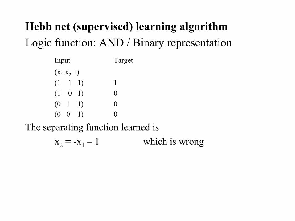
Hebb net (supervised) learning algorithm Logic function: AND / Binary representation Input Target
(x1 x2 1) (1 1 1) 1 (1 0 1) 0
(0 1 1) 0 (0 0 1) 0
The separating function learned is x2 = -x1 – 1 which is wrong
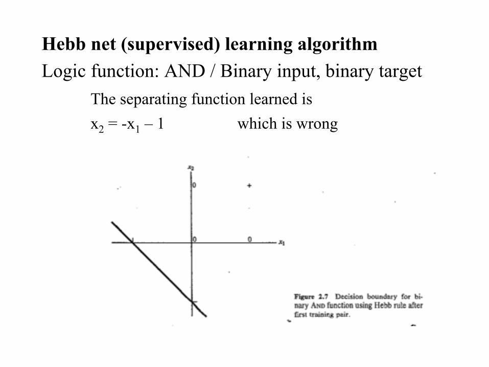
Hebb net (supervised) learning algorithm Logic function: AND / Binary input, binary target The separating function learned is
x2 = -x1 – 1 which is wrong
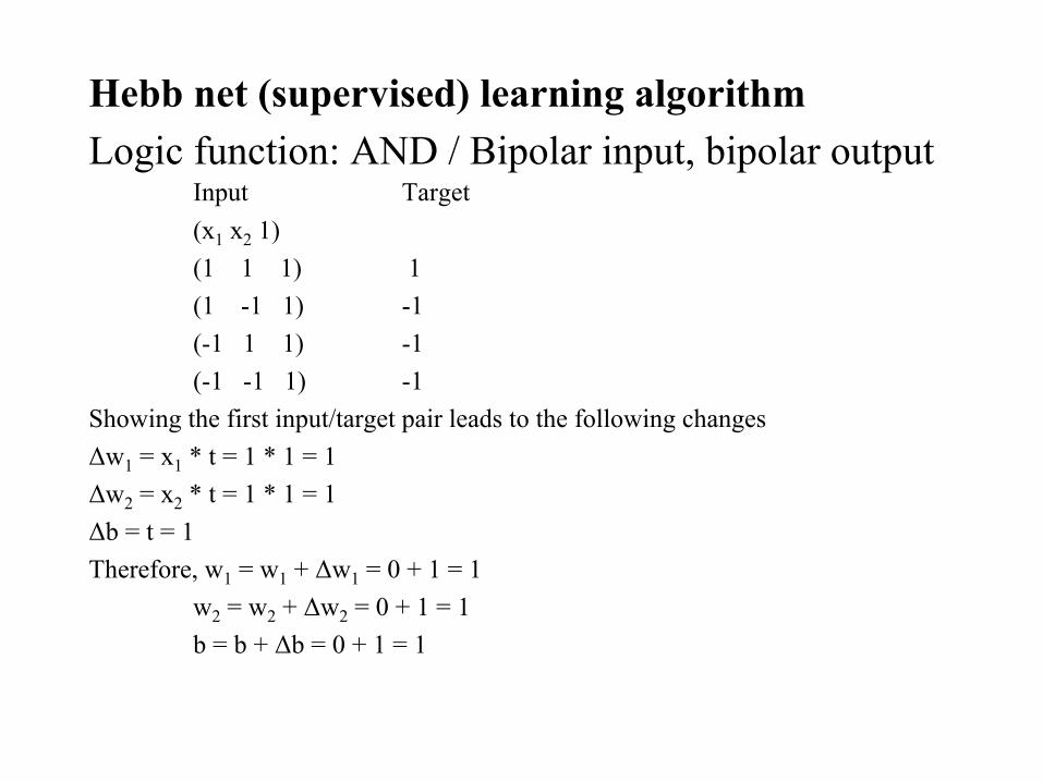
Hebb net (supervised) learning algorithm Logic function: AND / Bipolar input, bipolar output
Input Target (x1 x2 1) (1 1 1) 1 (1 -1 1) -1
(-1 1 1) -1 (-1 -1 1) -1 Showing the first input/target pair leads to the following changes Δw1 = x1 * t = 1 * 1 = 1 Δw2 = x2 * t = 1 * 1 = 1 Δb = t = 1 Therefore, w1 = w1 + Δw1 = 0 + 1 = 1
w2 = w2 + Δw2 = 0 + 1 = 1 b = b + Δb = 0 + 1 = 1
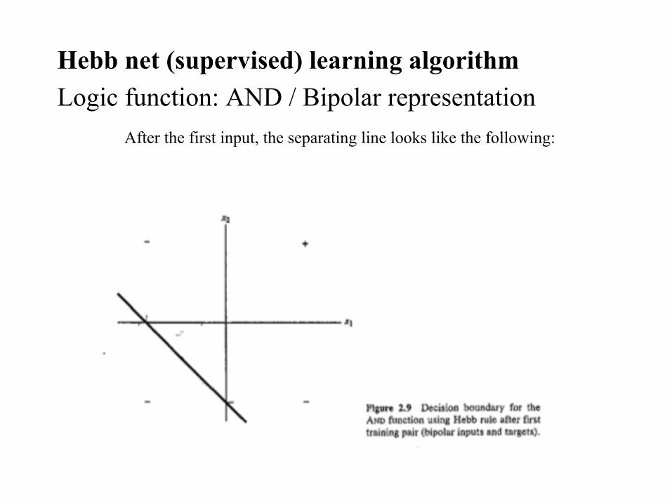
Hebb net (supervised) learning algorithm Logic function: AND / Bipolar representation After the first input, the separating line looks like the following:
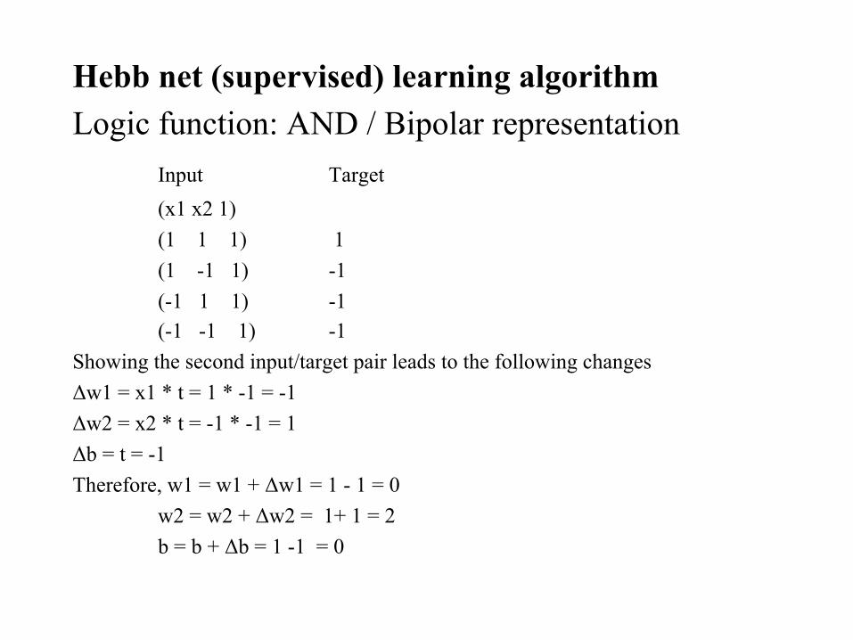
Hebb net (supervised) learning algorithm Logic function: AND / Bipolar representation Input Target
(x1 x2 1) (1 1 1) 1 (1 -1 1) -1
(-1 1 1) -1 (-1 -1 1) -1 Showing the second input/target pair leads to the following changes Δw1 = x1 * t = 1 * -1 = -1 Δw2 = x2 * t = -1 * -1 = 1 Δb = t = -1 Therefore, w1 = w1 + Δw1 = 1 - 1 = 0
w2 = w2 + Δw2 = 1+ 1 = 2 b = b + Δb = 1 -1 = 0
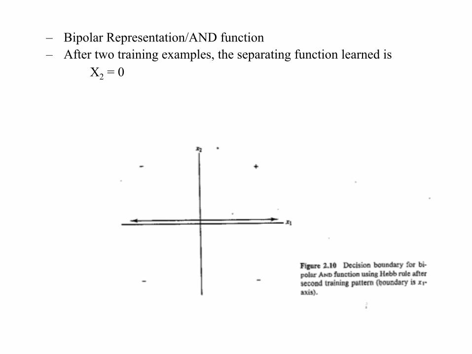
– Bipolar Representation/AND function – After two training examples, the separating function learned is
X2 = 0
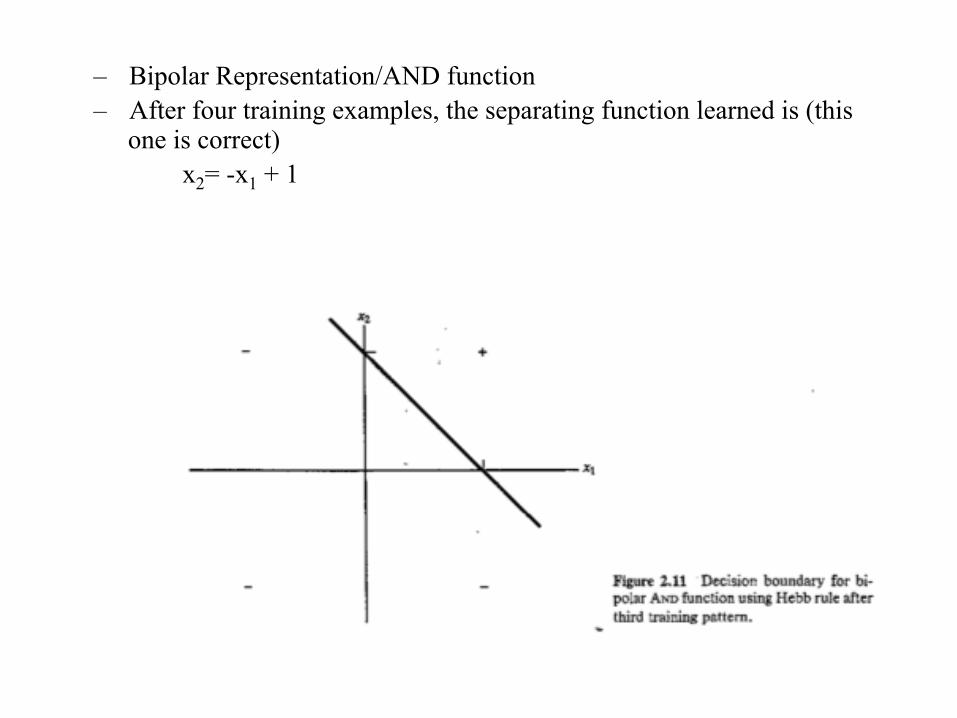
– Bipolar Representation/AND function – After four training examples, the separating function learned is (this
one is correct) x2= -x1 + 1
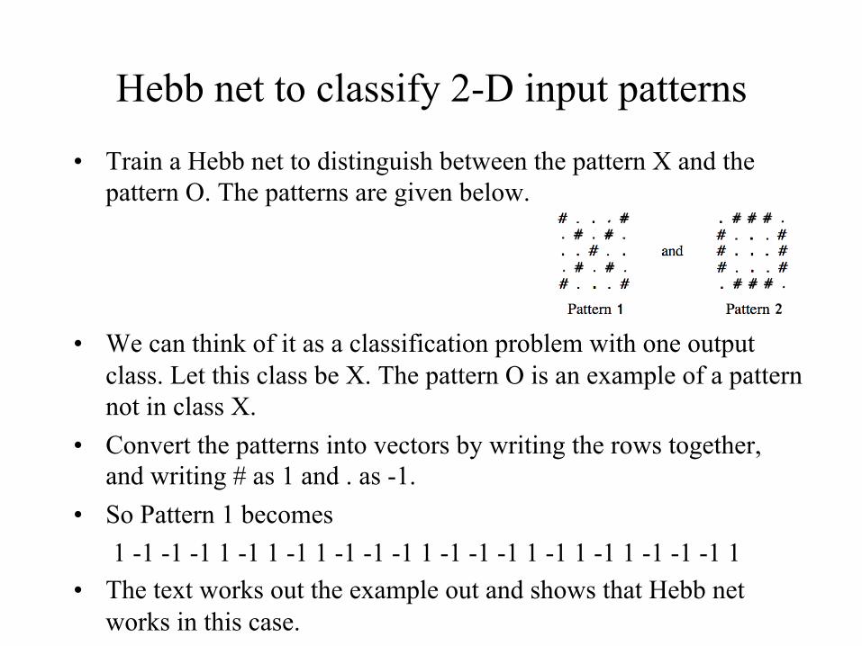
Hebb net to classify 2-D input patterns
• Train a Hebb net to distinguish between the pattern X and the pattern O. The patterns are given below.
• We can think of it as a classification problem with one output class. Let this class be X. The pattern O is an example of a pattern not in class X.
• Convert the patterns into vectors by writing the rows together, and writing # as 1 and . as -1.
• So Pattern 1 becomes 1 -1 -1 -1 1 -1 1 -1 1 -1 -1 -1 1 -1 -1 -1 1 -1 1 -1 1 -1 -1 -1 1 • The text works out the example out and shows that Hebb net
works in this case.
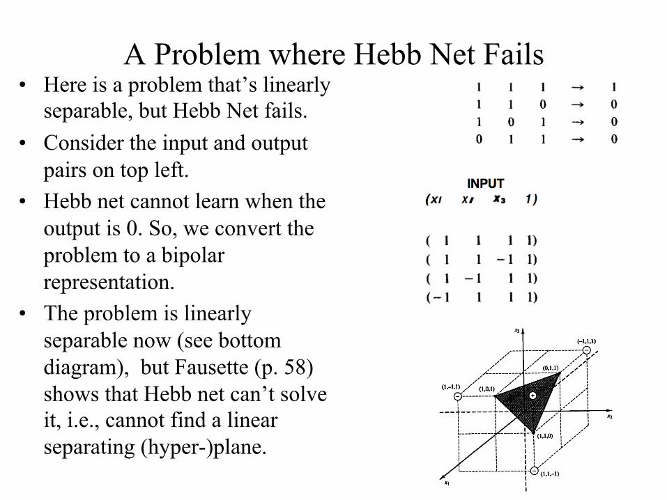
A Problem where Hebb Net Fails • Here is a problem that’s linearly
separable, but Hebb Net fails. • Consider the input and output
pairs on top left. • Hebb net cannot learn when the
output is 0. So, we convert the problem to a bipolar representation.
• The problem is linearly separable now (see bottom diagram), but Fausette (p. 58) shows that Hebb net can’t solve it, i.e., cannot find a linear separating (hyper-)plane.
Perceptrons
• Rosenblatt, a psychologist, proposed the perceptron model in 1958.
• Like the Hebbian model, it had weights on the connections.
• Learning took place by adapting the weights of the network.
• Rosenblatt’s model was refined in the the 1960s by Minsky and Papert and its computational properties were analyzed carefully.
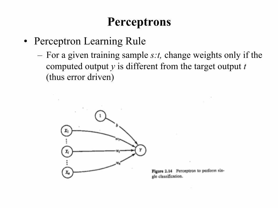
Perceptrons • Perceptron Learning Rule
– For a given training sample s:t, change weights only if the computed output y is different from the target output t (thus error driven)
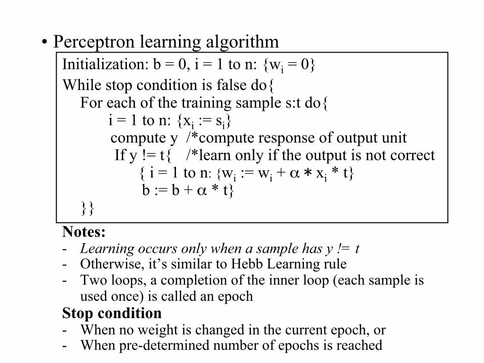
• Perceptron learning algorithm Initialization: b = 0, i = 1 to n: {wi = 0} While stop condition is false do{
For each of the training sample s:t do{ i = 1 to n: {xi := si}
compute y /*compute response of output unit If y != t{ /*learn only if the output is not correct
{ i = 1 to n: {wi := wi + α * xi * t} b := b + α * t}
}} Notes: - Learning occurs only when a sample has y != t - Otherwise, it’s similar to Hebb Learning rule - Two loops, a completion of the inner loop (each sample is
used once) is called an epoch Stop condition - When no weight is changed in the current epoch, or - When pre-determined number of epochs is reached
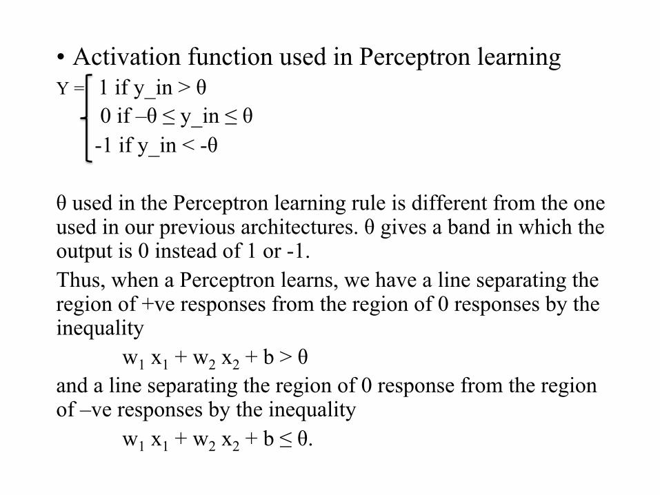
• Activation function used in Perceptron learning Y = 1 if y_in > θ 0 if –θ ≤ y_in ≤ θ -1 if y_in < -θ θ used in the Perceptron learning rule is different from the one used in our previous architectures. θ gives a band in which the output is 0 instead of 1 or -1. Thus, when a Perceptron learns, we have a line separating the region of +ve responses from the region of 0 responses by the inequality
w1 x1 + w2 x2 + b > θ and a line separating the region of 0 response from the region of –ve responses by the inequality
w1 x1 + w2 x2 + b ≤ θ.
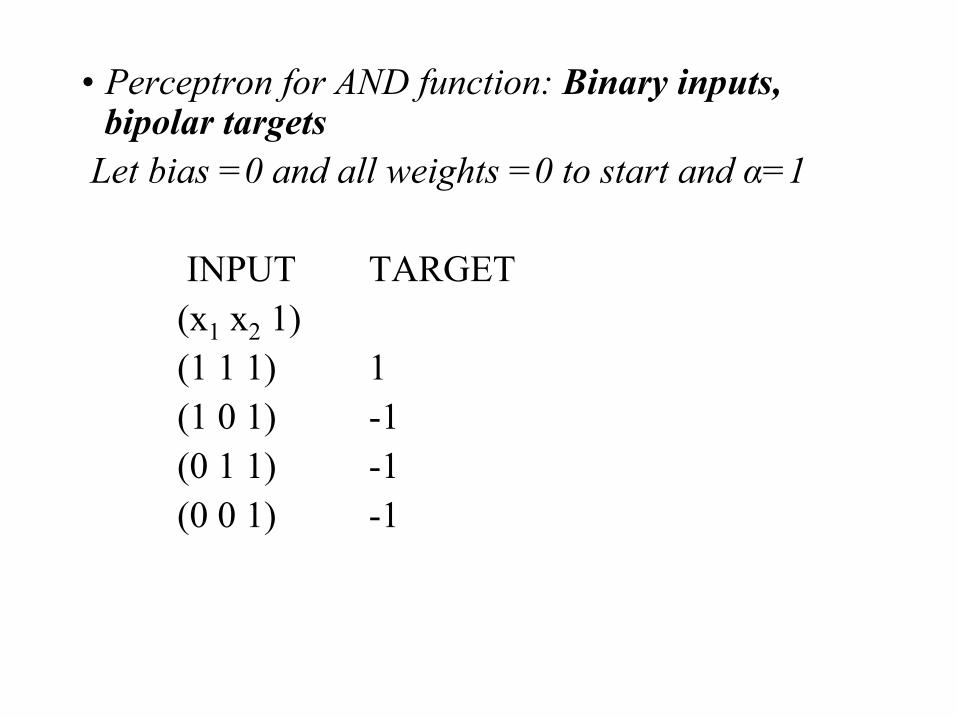
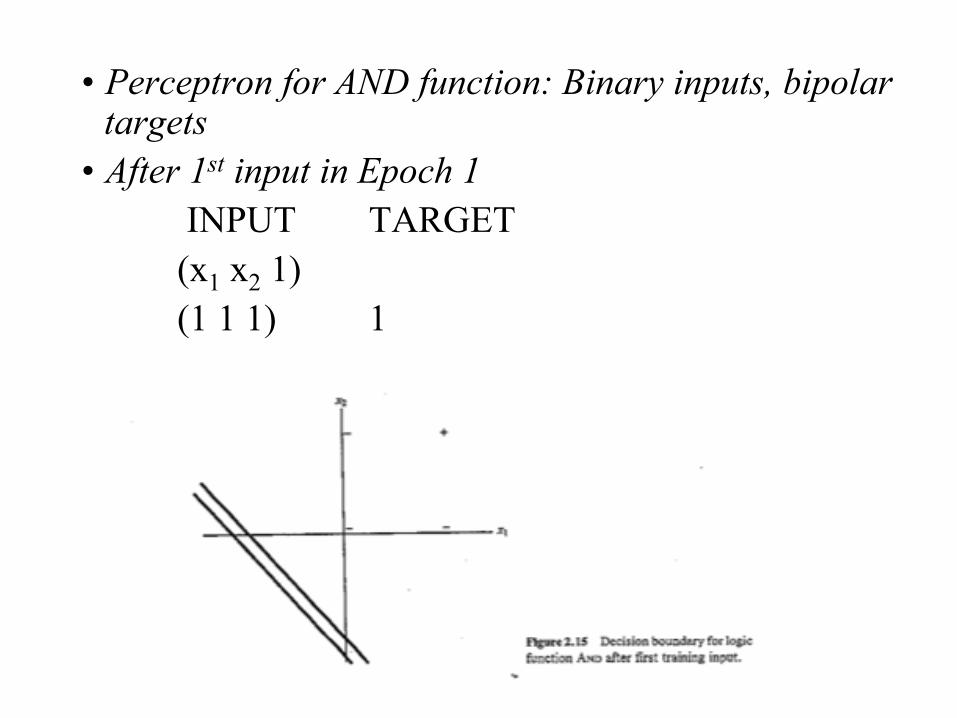
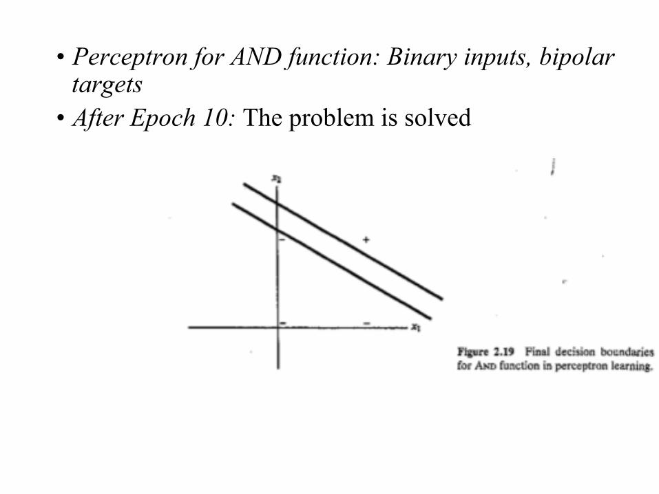
• Perceptron for AND function: Binary inputs, bipolar targets
Let bias =0 and all weights =0 to start and α=1
INPUT TARGET (x1 x2 1) (1 1 1) 1 (1 0 1) -1 (0 1 1) -1 (0 0 1) -1
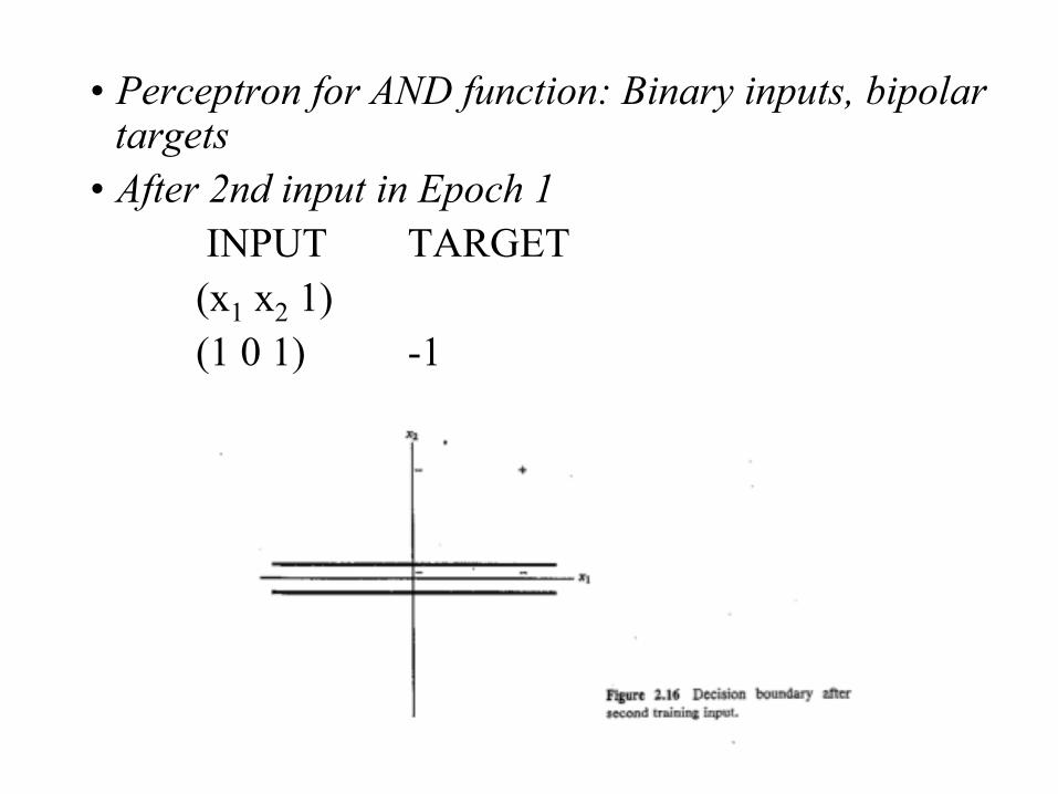
• Perceptron for AND function: Binary inputs, bipolar targets
• After 1st input in Epoch 1 INPUT TARGET (x1 x2 1) (1 1 1) 1
• Perceptron for AND function: Binary inputs, bipolar targets
• After 2nd input in Epoch 1 INPUT TARGET (x1 x2 1) (1 0 1) -1
• Perceptron for AND function: Binary inputs, bipolar targets
• After 3rd and 4th inputs in Epoch 1 INPUT TARGET (x1 x2 1) (0 1 1) -1 (0 0 1) -1
The weights change and hence we continue to a second epoch.
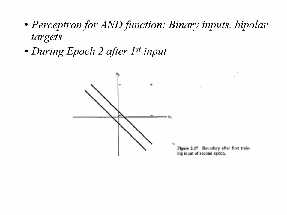
• Perceptron for AND function: Binary inputs, bipolar targets
• During Epoch 2 after 1st input
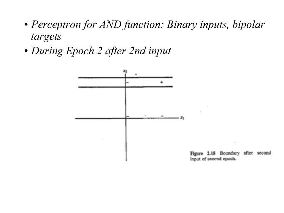
• Perceptron for AND function: Binary inputs, bipolar targets
• During Epoch 2 after 2nd input
• Perceptron for AND function: Binary inputs, bipolar targets
• After Epoch 10: The problem is solved
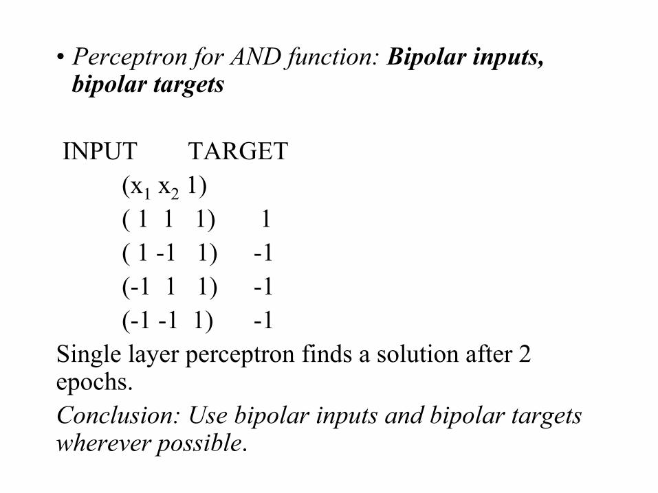
• Perceptron for AND function: Bipolar inputs, bipolar targets
INPUT TARGET (x1 x2 1) ( 1 1 1) 1 ( 1 -1 1) -1 (-1 1 1) -1 (-1 -1 1) -1
Single layer perceptron finds a solution after 2 epochs. Conclusion: Use bipolar inputs and bipolar targets wherever possible.
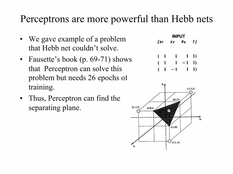
Perceptrons are more powerful than Hebb nets
• We gave example of a problem that Hebb net couldn’t solve.
• Fausette’s book (p. 69-71) shows that Perceptron can solve this problem but needs 26 epochs of training.
• Thus, Perceptron can find the separating plane.
Perceptrons Are More Powerful Than Hebb Nets
• Minsky and Pappert show that perceptrons are more powerful than Hebb Nets
• This is because a Perceptron uses iterative updating of weights through epochs and doesn’t stop training after only one showing of the inputs.
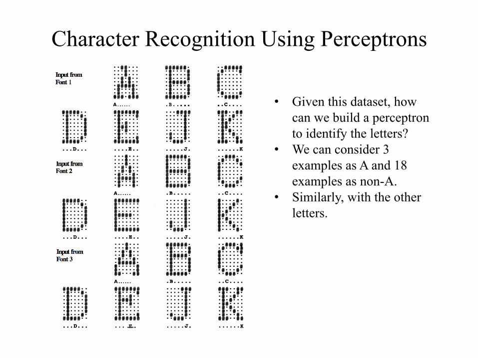
Character Recognition Using Perceptrons
• Given this dataset, how can we build a perceptron to identify the letters?
• We can consider 3 examples as A and 18 examples as non-A.
• Similarly, with the other letters.
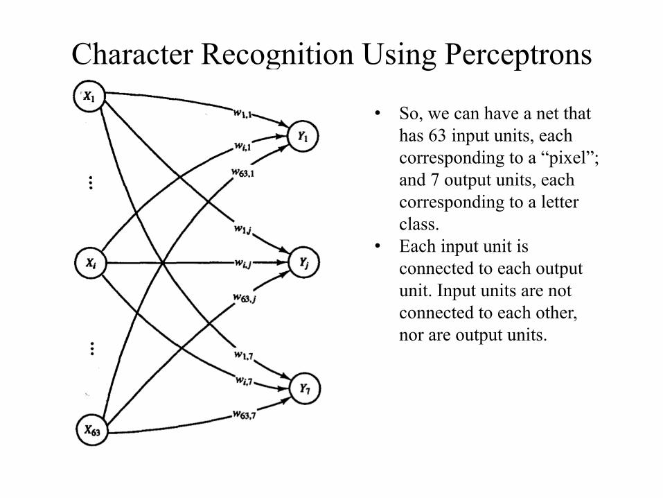
Character Recognition Using Perceptrons
• So, we can have a net that has 63 input units, each corresponding to a “pixel”; and 7 output units, each corresponding to a letter class.
• Each input unit is connected to each output unit. Input units are not connected to each other, nor are output units.
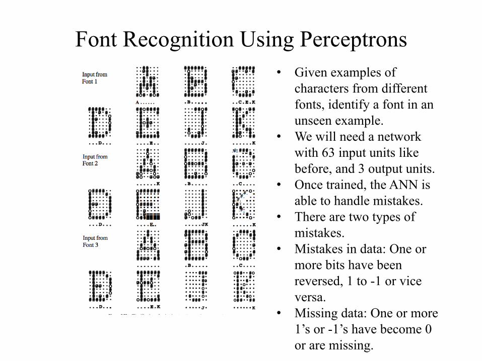
Font Recognition Using Perceptrons • Given examples of
characters from different fonts, identify a font in an unseen example.
• We will need a network with 63 input units like before, and 3 output units.
• Once trained, the ANN is able to handle mistakes.
• There are two types of mistakes.
• Mistakes in data: One or more bits have been reversed, 1 to -1 or vice versa.
• Missing data: One or more 1’s or -1’s have become 0 or are missing.
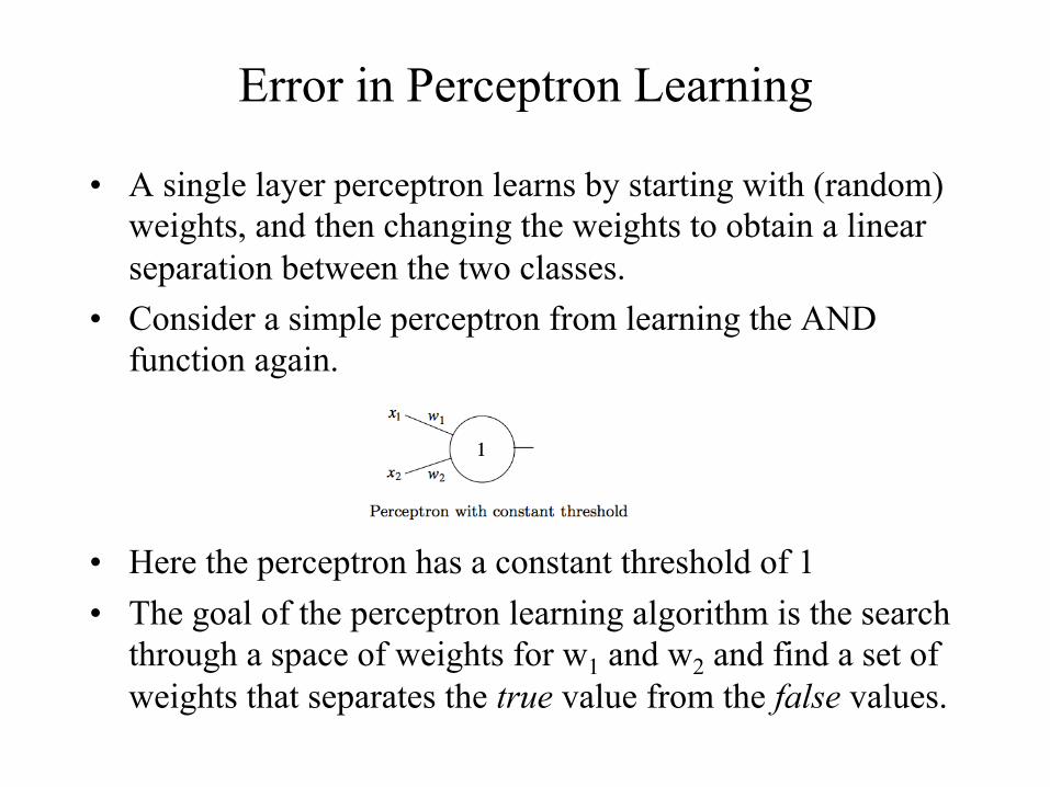
Error in Perceptron Learning
• A single layer perceptron learns by starting with (random) weights, and then changing the weights to obtain a linear separation between the two classes.
• Consider a simple perceptron from learning the AND function again.
• Here the perceptron has a constant threshold of 1 • The goal of the perceptron learning algorithm is the search
through a space of weights for w1 and w2 and find a set of weights that separates the true value from the false values.
Error in Perceptron Learning
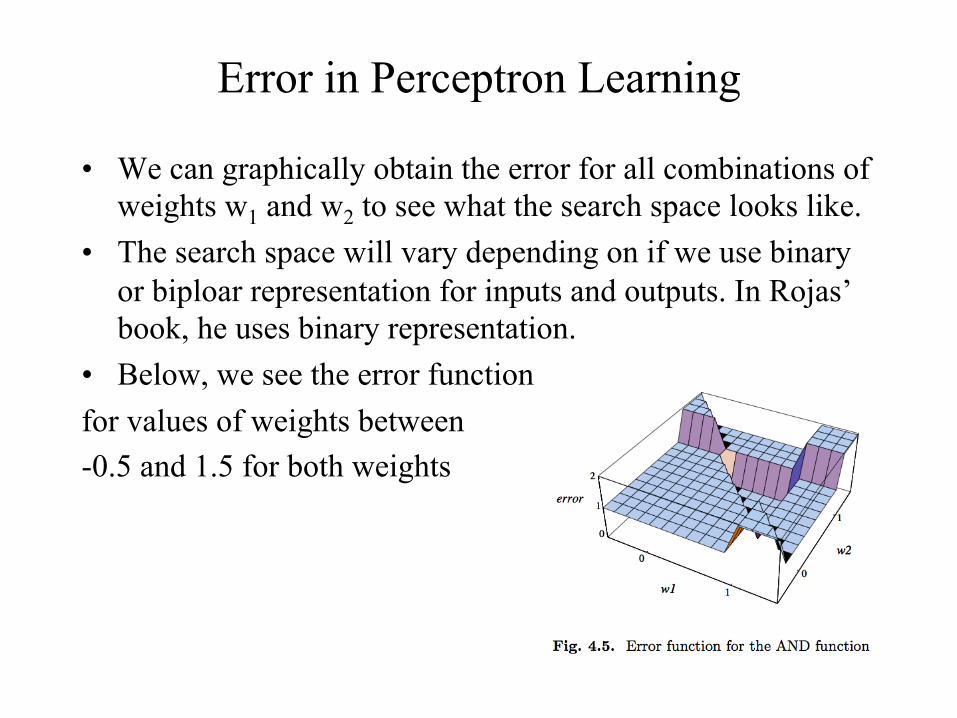
• We can graphically obtain the error for all combinations of weights w1 and w2 to see what the search space looks like.
• The search space will vary depending on if we use binary or biploar representation for inputs and outputs. In Rojas’ book, he uses binary representation.
• Below, we see the error function for values of weights between -0.5 and 1.5 for both weights
Error in Perceptron Learning
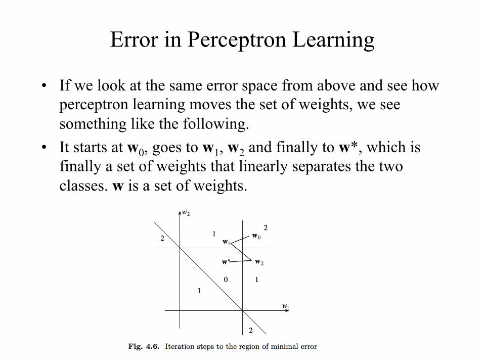
• If we look at the same error space from above and see how perceptron learning moves the set of weights, we see something like the following.
• It starts at w0, goes to w1, w2 and finally to w*, which is finally a set of weights that linearly separates the two classes. w is a set of weights.
Error in Perceptron Learning
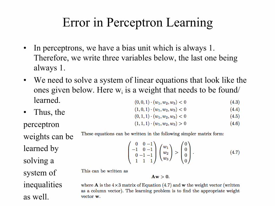
• In perceptrons, we have a bias unit which is always 1. Therefore, we write three variables below, the last one being always 1.
• We need to solve a system of linear equations that look like the ones given below. Here wi is a weight that needs to be found/learned.
• Thus, the perceptron weights can be learned by solving a system of inequalities as well.
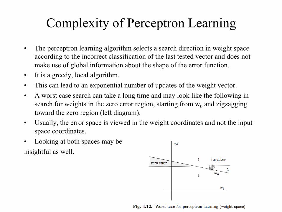
Complexity of Perceptron Learning
• The perceptron learning algorithm selects a search direction in weight space according to the incorrect classification of the last tested vector and does not make use of global information about the shape of the error function.
• It is a greedy, local algorithm. • This can lead to an exponential number of updates of the weight vector. • A worst case search can take a long time and may look like the following in
search for weights in the zero error region, starting from w0 and zigzagging toward the zero region (left diagram).
• Usually, the error space is viewed in the weight coordinates and not the input space coordinates.
• Looking at both spaces may be insightful as well.
Complexity of Perceptron Learning
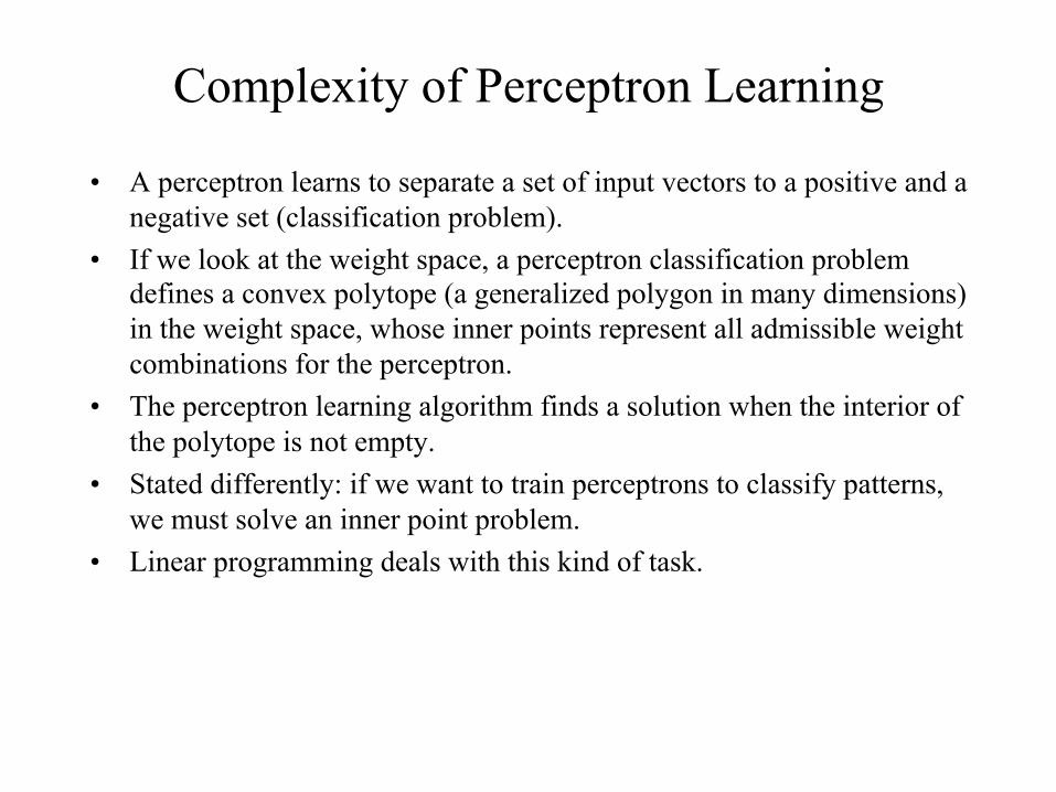
• A perceptron learns to separate a set of input vectors to a positive and a negative set (classification problem).
• If we look at the weight space, a perceptron classification problem defines a convex polytope (a generalized polygon in many dimensions) in the weight space, whose inner points represent all admissible weight combinations for the perceptron.
• The perceptron learning algorithm finds a solution when the interior of the polytope is not empty.
• Stated differently: if we want to train perceptrons to classify patterns, we must solve an inner point problem.
• Linear programming deals with this kind of task.
Complexity of Perceptron Learning
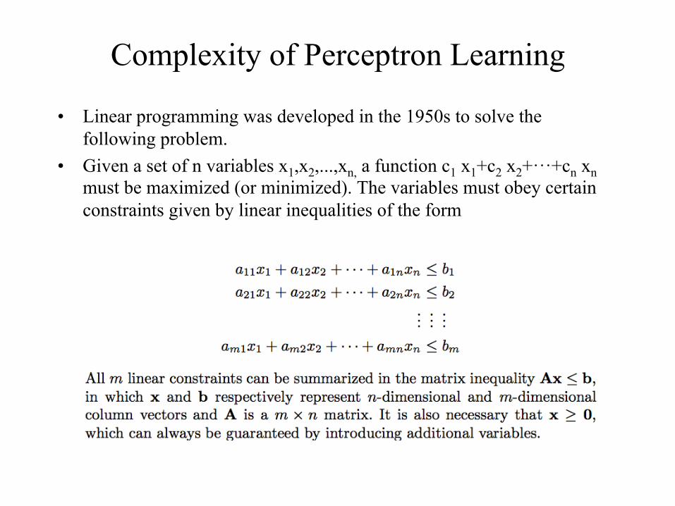
• Linear programming was developed in the 1950s to solve the following problem.
• Given a set of n variables x1,x2,...,xn, a function c1 x1+c2 x2+···+cn xn must be maximized (or minimized). The variables must obey certain constraints given by linear inequalities of the form
Complexity of Perceptron Learning
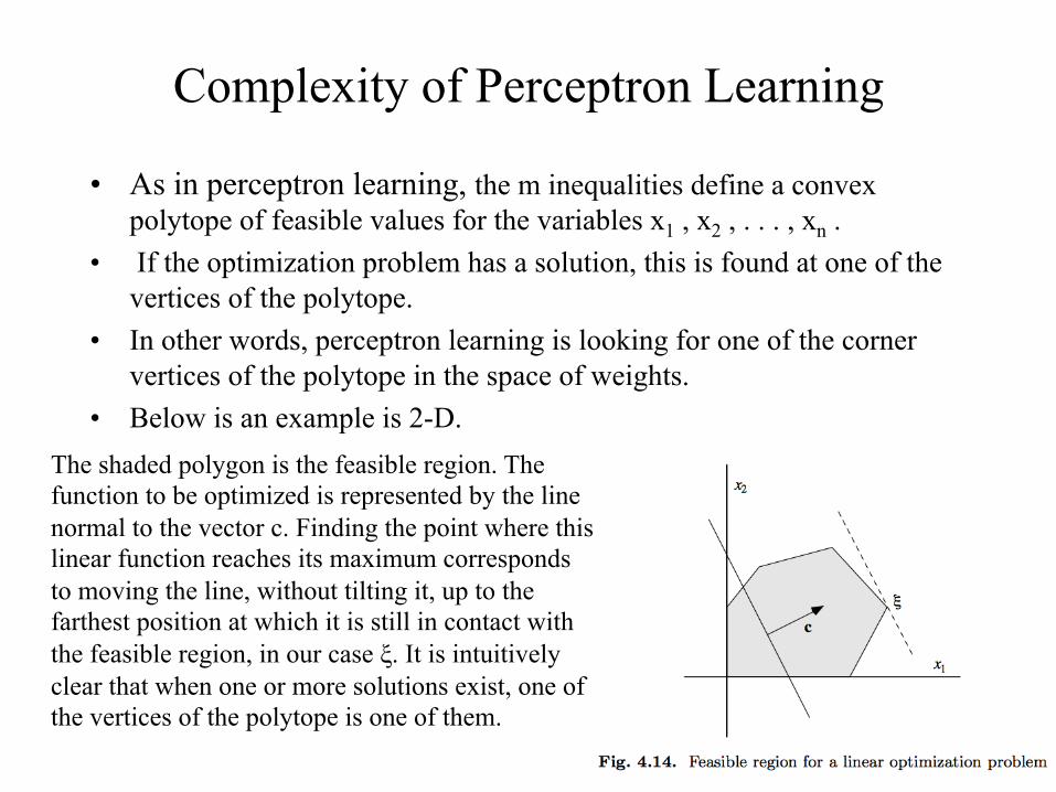
• As in perceptron learning, the m inequalities define a convex polytope of feasible values for the variables x1 , x2 , . . . , xn .
• If the optimization problem has a solution, this is found at one of the vertices of the polytope.
• In other words, perceptron learning is looking for one of the corner vertices of the polytope in the space of weights.
• Below is an example is 2-D. The shaded polygon is the feasible region. The function to be optimized is represented by the line normal to the vector c. Finding the point where this linear function reaches its maximum corresponds to moving the line, without tilting it, up to the farthest position at which it is still in contact with the feasible region, in our case ξ. It is intuitively clear that when one or more solutions exist, one of the vertices of the polytope is one of them.
Complexity of Perceptron Learning • The well-known simplex algorithm of linear programming starts at a
vertex of the feasible region and jumps to another neighboring vertex, always moving in a direction in which the function to be optimized increases.
• In the worst case an exponential number of vertices in the number of inequalities m has to be traversed before a solution is found.
• In other words, the worst case complexity is exponential on the number of inequalities.
• See http://myweb.clemson.edu/~pbelott/bulk/teaching/mthsc440/lecture07.pdf for a proof
• On average, however, the simplex algorithm is not so inefficient.
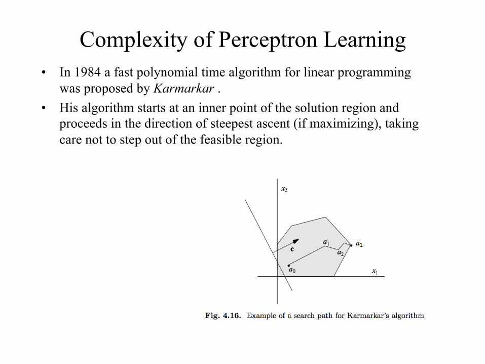
Complexity of Perceptron Learning • In 1984 a fast polynomial time algorithm for linear programming
was proposed by Karmarkar . • His algorithm starts at an inner point of the solution region and
proceeds in the direction of steepest ascent (if maximizing), taking care not to step out of the feasible region.
Complexity of Perceptron Learning • In the worst case Karmarkar’s algorithm executes in a number of iterations
proportional to n3.5, where n is the number of variables in the problem and other factors are kept constant.
• Published modifications of Karmarkar’s algorithm are still more efficient. • However, such algorithms start beating the simplex method in the average
case only when the number of variables and constraints becomes relatively large, since the computational overhead for a small number of constraints is not negligible.
• The existence of a polynomial time algorithm for linear programming and for the solution of interior point problems shows that perceptron learning is not what is called a hard (NP-complete) computational problem.
• Given any number of training patterns, the learning algorithm (in this case linear programming) can decide whether the problem has a solution or not.
• If a solution exists, it finds the appropriate weights in polynomial time at most.
• Note: In other words, we can solve the Perceptron weights problem using simplex or Karmakar’s algorithm, without going through the “traditional” training process.
• Beyond Perceptron • Single layer Perceptrons cannot solve the XOR
problem, they can solve only linearly separable problems.
• Perceptron training stops as soon as all training patterns are classified correctly.
• It may be a better idea to have a learning procedure that could continue to improve its weights even after the classifications are correct.
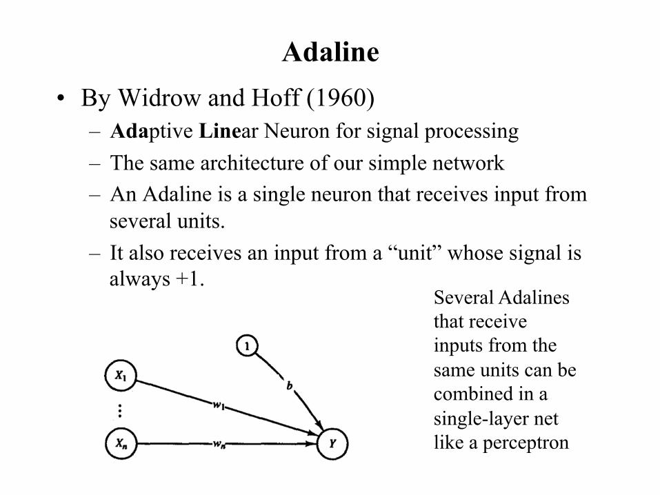
Adaline • By Widrow and Hoff (1960)
– Adaptive Linear Neuron for signal processing – The same architecture of our simple network – An Adaline is a single neuron that receives input from
several units. – It also receives an input from a “unit” whose signal is
always +1. Several Adalines that receive inputs from the same units can be combined in a single-layer net like a perceptron
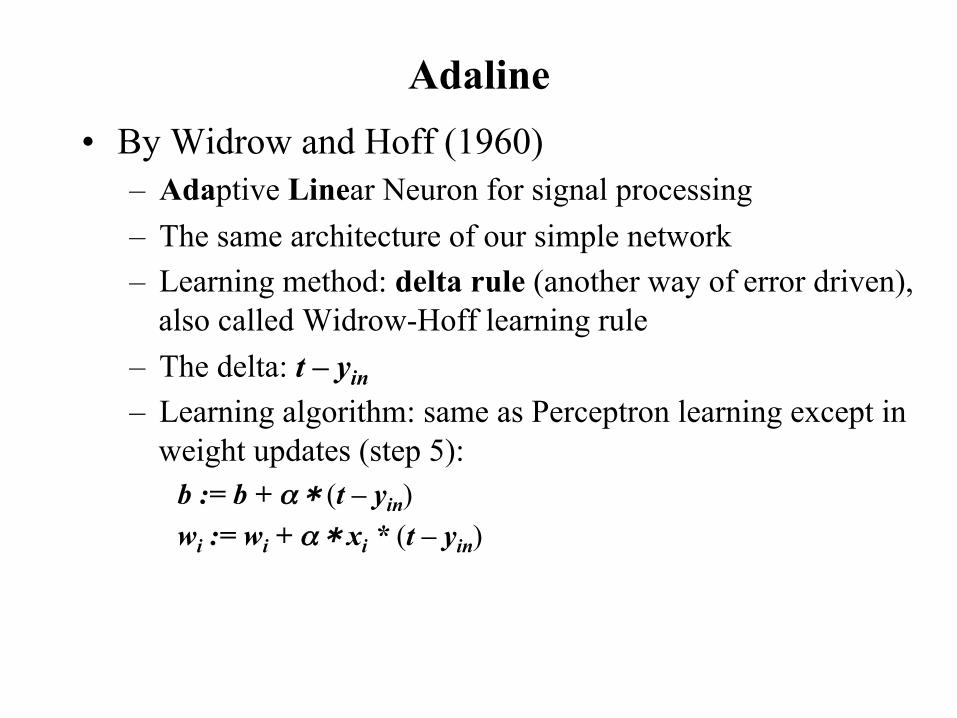
Adaline • By Widrow and Hoff (1960)
– Adaptive Linear Neuron for signal processing – The same architecture of our simple network – Learning method: delta rule (another way of error driven),
also called Widrow-Hoff learning rule – The delta: t – yin
– Learning algorithm: same as Perceptron learning except in weight updates (step 5):
b := b + α * (t – yin) wi := wi + α * xi * (t – yin)
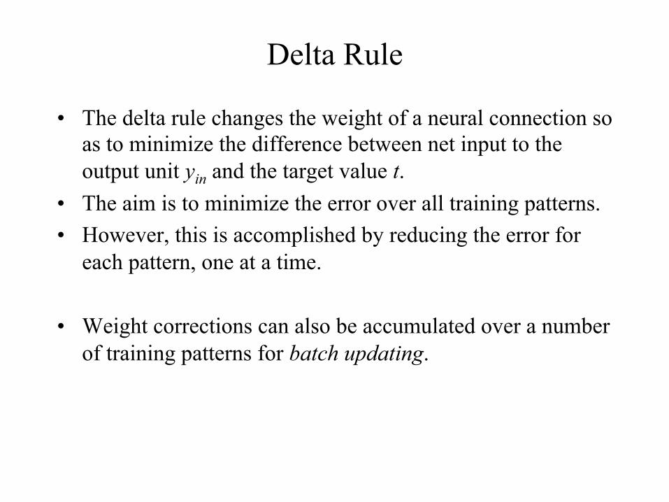
Delta Rule
• The delta rule changes the weight of a neural connection so as to minimize the difference between net input to the output unit yin and the target value t.
• The aim is to minimize the error over all training patterns. • However, this is accomplished by reducing the error for
each pattern, one at a time.
• Weight corrections can also be accumulated over a number of training patterns for batch updating.
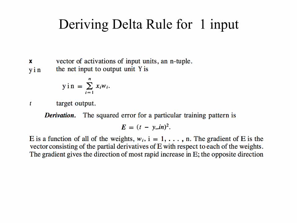
Deriving Delta Rule for 1 input
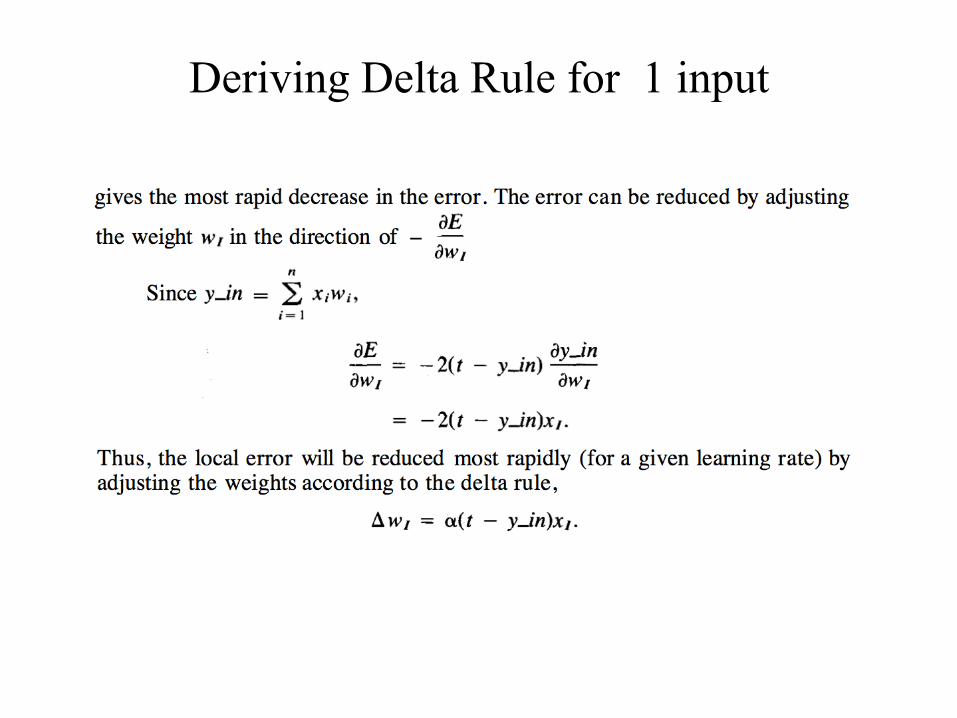
Deriving Delta Rule for 1 input
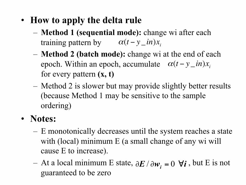
• How to apply the delta rule – Method 1 (sequential mode): change wi after each
training pattern by – Method 2 (batch mode): change wi at the end of each
epoch. Within an epoch, accumulate for every pattern (x, t)
– Method 2 is slower but may provide slightly better results (because Method 1 may be sensitive to the sample ordering)
• Notes: – E monotonically decreases until the system reaches a state
with (local) minimum E (a small change of any wi will cause E to increase).
– At a local minimum E state, , but E is not guaranteed to be zero
α(t − y_ in)xi
iwE i ∀=∂∂ 0/
α(t − y_ in)xi
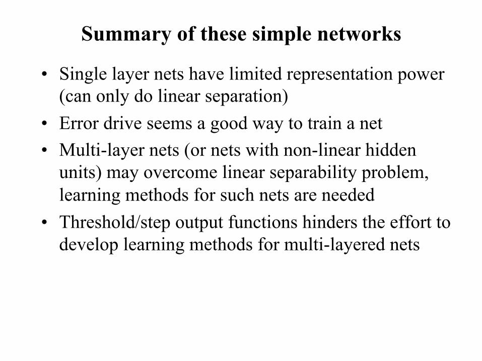
Summary of these simple networks
• Single layer nets have limited representation power (can only do linear separation)
• Error drive seems a good way to train a net • Multi-layer nets (or nets with non-linear hidden
units) may overcome linear separability problem, learning methods for such nets are needed
• Threshold/step output functions hinders the effort to develop learning methods for multi-layered nets