Embed Size (px)
Citation preview

ARTICLE IN PRESS
Journal of Financial Economics 79 (2006) 469–506
0304-405X/$
doi:10.1016/j
$We wou
Huang, Mik
Arizona Stat
Insurance Co
University of
(the referee)
helpful advic�CorrespoE-mail ad
www.elsevier.com/locate/jfec
Partial adjustment toward target capital structures$
Mark J. Flannerya,�, Kasturi P. Ranganb
aGraduate School of Business, University of Florida, Gainesville, FL 32611-7168, USAbWeatherhead School of Management, Case Western Reserve University, Cleveland, OH 44106, USA
Received 12 May 2004; received in revised form 21 December 2004; accepted 16 March 2005
Available online 10 October 2005
Abstract
The empirical literature provides conflicting assessments about how firms choose their capital
structures. Distinguishing among the three main hypotheses (‘‘tradeoff’’, pecking order, and market
timing) requires that we know whether firms have long-run leverage targets and (if so) how quickly
they adjust toward them. Yet many previous researchers have applied empirical specifications that
fail to recognize the potential for incomplete adjustment. A more general, partial-adjustment model
of firm leverage indicates that firms do have target capital structures. The typical firm closes about
one-third of the gap between its actual and its target debt ratios each year.
r 2005 Elsevier B.V. All rights reserved.
JEL classification: G 32
Keywords: Leverage; Tradeoff theory; Target; Speed of adjustment
1. Introduction
Since Modigliani and Miller’s irrelevance proposition in 1958 (Modigliani and Miller,1958), researchers have investigated firms’ decisions about how to finance their operations.
- see front matter r 2005 Elsevier B.V. All rights reserved.
.jfineco.2005.03.004
ld like to thank, without implicating, Jay Ritter, Artuno Bris, Ralf Elsas, Vidhan Goyal, Rongbing
e Lemmon, Peter MacKay, Sam Thomas, Ivo Welch, Jeff Wurgler, and seminar participants at
e University, the Atlanta Finance Forum, Case Western Reserve University, the Federal Deposit
rporation, George Mason University, New York University, Southern Methodist University, the
Texas, and Washington University for comments on previous drafts of this paper. Murray Frank
provided advice that substantially improved the paper. George Pennacchi and Ajai Singh provided
e about a related paper.
nding author. Tel.: 352 392 3184; fax: 352 392 0301.
dress: [email protected] (M.J. Flannery).
ARTICLE IN PRESSM.J. Flannery, K.P. Rangan / Journal of Financial Economics 79 (2006) 469–506470
Initially, they asked whether the irrelevance proposition is consistent with the availabledata, or, whether instead capital market imperfections make firm value depend on capitalstructure. In the latter case, it was argued, firms would select target debt-equity ratios,trading off their costs and benefits of leverage. Survey evidence by Graham and Harvey(2001) shows that indeed, 81% of firms consider a target debt ratio or range when makingtheir debt decisions. However, alternative theories remain plausible. Myers (1984)contrasts this tradeoff theory of capital structure with an updated version of Donaldson’s(1961) pecking order theory, according to which information asymmetries lead managersto perceive that the market generally underprices their shares. Accordingly, investmentsare financed first with internally generated funds, the firm issues safe debt if internal fundsprove insufficient, and equity is used only as a last resort. In a pecking order world,observed leverage reflects primarily a firm’s historical profitability and investmentopportunities. Firms have no strong preference about their leverage ratios and, a fortiori,no strong inclination to reverse leverage changes caused by financing needs or earningsgrowth.Two additional theories of capital structure also reject the notion of timely convergence
toward a target leverage ratio. First, Baker and Wurgler (2002) argue that a firm’sobserved capital structure reflects its cumulative ability to sell overpriced equity shares:that is, share prices fluctuate around their ‘‘true’’ values, and managers tend to issue shareswhen the firm’s market-to-book ratio is high. Unlike the pecking order hypothesis, thismarket timing hypothesis asserts that managers routinely exploit information asymmetriesto benefit current shareholders; like the pecking order hypothesis, there is no reversion to atarget capital ratio if market timing is the dominant influence on firm leverage. Second,Welch (2004) argues that managerial inertia permits stock price changes to have aprominent effect on market-valued debt ratios: ‘‘... over reasonably long time frames, thestock price effects are considerably more important in explaining debt-equity ratios thanpreviously identified proxies’’ (p. 107).The pecking order, market timing, and inertia theories of capital structure imply that
managers perceive no great leverage effect on firm value and therefore make no effort toreverse changes in leverage. In contrast, the tradeoff theory maintains that marketimperfections generate a link between leverage and firm value, and firms take positive stepsto offset deviations from their optimal debt ratios. The speed with which firms reversedeviations from their target debt ratios depends on the cost of adjusting leverage. Withzero adjustment costs, the tradeoff theory implies that firms should never deviate fromtheir optimal leverage. At the other extreme, if transaction costs are infinite we shouldobserve no movements toward a target. Baker and Wurgler (2002) emphasize theconnection between adjustment costs and observed capital structure:
The basic question is whether market timing has a short-run or a long-run impact.One expects at least a mechanical, short-run impact. However, if firms subsequently
rebalance away from the influence of market timing financing decisions, as normative
capital structure theory recommends, then market timing would have no persistentimpact on capital structure. (page 2, emphasis added)
Estimating the effect of capital adjustment costs is thus a key first step in testingcompeting theories of capital structure.The empirical model in this paper accounts for the potentially dynamic nature of a firm’s
capital structure. The model is general enough that we can test whether there is indeed a

ARTICLE IN PRESSM.J. Flannery, K.P. Rangan / Journal of Financial Economics 79 (2006) 469–506 471
leverage target and if so, what is the (adjustment) speed with which a firm moves toward itstarget. Our evidence indicates that firms do target a long run capital structure, and that thetypical firm converges toward its long-run target at a rate of more than 30% per year. Thisadjustment speed is roughly three times faster than many existing estimates in theliterature, and affords targeting behavior an empirically important effect on firms’observed capital structures. When we add market timing or pecking order variables to ourbase specification, we do find some support for these theories. However, more than half ofthe observed changes in capital structures can be attributed to targeting behavior whilemarket timing and pecking order considerations explain less than 10% each. Unlike Welch(2004), we find that stock price changes have only transitory effects on capital structure.
Our findings are not consistent with many recent empirical papers on capital structure(e.g., Shyam-Sunder and Myers, 1999; Baker and Wurgler, 2002; Fama and French, 2002;Huang and Ritter, 2005; Welch, 2004). However, the literature also offers some precedentsfor our rapid estimated adjustment speeds (Marcus, 1983; Jalilvand and Harris, 1984;Roberts, 2002). We argue that some previous empirical models impose unwarranted, yettestable, assumptions about the adjustment speed and/or the dynamic properties of targetleverage. These assumptions materially influence the estimation results and consequentlythe conclusions drawn. Part of our paper’s contribution is to identify why previousresearch produces such disparate estimated adjustment speeds.
The paper is organized as follows. Section 2 derives our preferred regressionspecification for testing the tradeoff theory in a partial adjustment framework. Section 3describes the Compustat—CRSP data we use to estimate our regression models. Section 4presents our basic results. After showing that our regressions are robust to variousestimation methods, we establish the statistical and economic significance of a target debtratio and relate our results to previous discussions of the tradeoff theory. Section 5explicitly compares our model to the pecking order, market timing, and inertia models.Section 6 presents a series of robustness tests and the final section concludes. An appendixdiscusses the econometric issues associated with estimating the dynamic panel regressionthat constitutes our base specification.
2. Regression model specification
A regression specification used to test for tradeoff leverage behavior must permit eachfirm’s target debt ratio to vary over time, and must recognize that deviations from targetleverage are not necessarily offset quickly. Both of these requirements are satisfied in amodel with partial (incomplete) adjustment toward a target leverage ratio that depends onfirm characteristics.
2.1. Target leverage
Our primary leverage measure is a firm’s market debt ratio,1
MDRi;t ¼Di;t
Di;t þ Si;tPi;t, (1)
1Finance theory tends to downplay the importance of book ratios, with previous research largely analyzing
market-valued debt ratios (including Hovakimian et al., 2001; Hovakimian, 2003; Fama and French, 2002; Welch,

ARTICLE IN PRESSM.J. Flannery, K.P. Rangan / Journal of Financial Economics 79 (2006) 469–506472
where Di,t denotes the book value of firm i’s interest-bearing debt (the sum of Compustatitems 9 plus 34) at time t, Si,t equals the number of common shares outstanding (Compustatitem 199) at time t, and Pi,t denotes the price per share (Compustat item 25) at time t.We model the possibility that target leverage might differ across firms or over time by
specifying a target capital ratio of the form
MDR�i;tþ1 ¼ bX i;t, (2)
where MDR�i;tþ1 is firm i’s desired debt ratio at t+1, Xi,t is a vector of firm characteristicsrelated to the costs and benefits of operating with various leverage ratios, and b is acoefficient vector. Under the tradeoff hypothesis, b6¼0, and the variation in MDR�i;tþ1should be nontrivial.
2.2. Adjustment to target leverage
In a frictionless world, firms would always maintain their target leverage. However,adjustment costs may prevent immediate adjustment to a firm’s target, as the firm tradesoff its adjustment costs against the costs of operating with suboptimal leverage. Weestimate a model that permits incomplete (partial) adjustment of the firm’s initial capitalratio toward its target within each time period. The data can then indicate a typicaladjustment speed.A standard partial adjustment model is given by
MDRi;tþ1 �MDRi;t ¼ lðMDR�i;tþ1 �MDRi;tÞ þ~di;tþ1. (3)
Each year, the typical firm closes a proportion l of the gap between its actual and itsdesired leverage levels. Substituting (2) into (3) and rearranging gives the estimable model
MDRi;tþ1 ¼ ðlbÞX i;t þ ð1� lÞMDRi;t þ~di;tþ1. (4)
Eq. (4) says that managers take ‘action’ or ‘steps’ to close the gap between where they are(MDRi;t) and where they wish to be (b Xi,t). The specification further implies that
(1)
(foo
2004
gene
are2W
Alth
stati
coef
The firm’s actual debt ratio eventually converges to its target debt ratio, bX i;t.
(2) The long-run impact of Xi,t on the capital ratio is given by its estimated coefficient,divided by l.
(3) All firms have the same adjustment speed (l).2The smooth partial adjustment in Eq. (4) may only approximate an individual firm’sactual adjustments. A reasonable alternative model would permit small deviations from
tnote continued)
; Leary and Roberts, 2005). When authors analyze both market and book leverage ratios, the results are
rally comparable. We report similar results below in Table 5. Table 11 presents evidence that our conclusions
robust across a range of reasonable definitions for ‘‘leverage.’’
e experiment with modeling l as a function of firm-specific variables (Y), that is,
MDRi;tþ1 ¼ ðlðY ÞbÞX i;t þ ð1� lðY ÞÞMDRi;t þ di;tþ1. (5)
ough we find some evidence that firm characteristics affect adjustment speeds (the coefficients on Y are
stically significant), we do not report this evidence here because the mean adjustment speeds (lðY Þ) and the
ficients on Xi,t are very similar to the results of estimating (4). Roberts (2002) analyzes this issue further.

ARTICLE IN PRESSM.J. Flannery, K.P. Rangan / Journal of Financial Economics 79 (2006) 469–506 473
the target to persist because adjustment costs outweigh the gains from removing smalldeviations between actual and target leverage (Fischer et al. (1989); Mauer and Triantis(1994); Titman and Tsyplakov (2004); Leary and Roberts (2005); Ju et al. (2002)). Indeed,Figs. 1 and 2 below indicate that the mean change in book leverage substantially exceedsthe median, a phenomenon also observed by Frank and Goyal (2003, p. 228), Leary andRoberts (2005); and Halov and Heider (2004, Table 1).
We investigate the impact of infrequent adjustments on the parameters estimated by oursmooth adjustment specification (4) by simulating 20 sets of panel data, each with 100,000data points. The data are generated by assuming that while each firm’s target changesstochastically every year, the actual debt ratio is adjusted only periodically. For therandomly chosen periods in which debt is adjusted, the simulated firm adjusts completelyto its target ratio. When we estimate a partial adjustment model on these generated datasets, we find that the estimated adjustment speed exceeds the true proportion of adjustingfirms by less than 2%. (That is, if an average of 30% of sample firms move to their targeteach year, the estimated adjustment speed is less than 0.306). The average bias isstatistically significant, but economically unimportant. We therefore interpret the
-3.12%
-0.47%
1.33%
4.69%
-4%
-2%
0%
2%
4%
6%
-15.29% -1.36% 6.35% 21.96%Mean Distance From Target (MDR* - MDR) in year t-1
Ch
ang
e in
Bo
ok
Deb
t Rat
io
MeanMedian
Fig. 1. Subsequent year’s change in book debt ratio.
-1.3%
-0.1%
1.5%
-0.9% -0.5% 0.0%-0.1%
-4%
0%
4%
HighestMDR
Quartile
<------------- --------------> LowestMDR
QuartileAbsolute MDR
Ch
ang
e in
Bo
ok
Deb
t R
atio
Mean
Median
3.4%
Fig. 2. Mean reversion in leverage.
ARTICLE IN PRESS
Table
1
Summary
statistics
Sampleincludes
allIndustrialCompustatfirm
swithcomplete
data
fortw
oormore
adjacentyears
during1965to
2001.Total:12,919firm
s;111,106firm
years.All
variablesare
winsorizedatthe1st
and99th
percentilesto
avoid
theinfluence
ofextrem
eobservations.
Number
of
observations
Mean
Median
Std.Dev.
Min.
Max.
MD
R111,106
0.2783
0.2252
0.2439
0.0000
0.9174
SP
E111,106
0.0038
0.0000
0.0917
�0.3383
0.4334
BD
R111,106
0.2485
0.2296
0.1925
0.0000
0.8635
EB
IT_
TA
111,106
0.0517
0.0935
0.2142
�1.6371
0.4096
MB
111,106
1.6153
1.0415
1.7888
0.2690
13.6372
DE
P_
TA
111,106
0.0451
0.0381
0.0327
0.0000
0.2338
LnT
A111,106
18.2400
18.1126
2.0184
12.7227
23.3787
FA
_TA
111,106
0.3220
0.2754
0.2200
0.0005
0.9220
R&
D_
DU
M111,106
0.4654
0.0000
0.4988
0.0000
1.0000
R&
D_
TA
111,106
0.0337
0.0000
0.0830
0.0000
0.8290
Ra
ted
111,106
0.1035
0.0000
0.3046
0.0000
1.0000
IND
_Med
ian
111,106
0.2240
0.2145
0.1339
0.0000
0.8164
MB
_EF
WA
81,343
1.7552
1.2828
1.3918
0.2690
9.9976
L3M
DR
98,709
0.2698
0.2289
0.2189
0.0000
0.9174
FIN
DE
F111,106
0.0818
0.0074
0.2228
�1.8180
2.4829
MD
R1
110,659
0.2110
0.1737
0.1848
0.0000
0.9918
MD
R2
111,093
0.4121
0.3979
0.2445
�0.0016
1.0000
MD
R3
108,995
0.2064
0.1459
0.2090
0.0000
1.6114
MD
R:
market
debt
ratio¼
book
value
of
(short-term
plus
long-term)
debt
(Compustat
item
s[9]+
[34])/m
arket
value
of
assets
(Compustat
item
s
[9]+
[34]+
[199]�[25])
SP
Et:thesurprise
impact
ofshare
price
changeonafirm
’sM
DR
during(t,
t+1).
SP
Et¼
Deb
t t
ðDeb
t tþ
Ma
rket
Eq
uit
ytð1þ~ R
t;tþ
1Þ
�� �
MD
Rt,
M.J. Flannery, K.P. Rangan / Journal of Financial Economics 79 (2006) 469–506474

ARTICLE IN PRESSwhere~ R
t;tþ
1istherealizedreturn
inthe
ithfirm
’sstock
betweentand
t+1.
BD
R:bookdebtratio:(long-term
[9]+
short-term
[34]debt)/totalassets[6].
EB
IT_
TA:profitability:earningsbefore
interest
andtaxes
(Compustatitem
s[18]+
[15]+
[16]),asaproportionoftotalassets(C
ompustatitem
[6]).
Ma
rket
Eq
uit
y:market
valueofoutstandingcommonstock
(Compustatitem
s[199�25]).
MB:market
tobookratioofassets:bookliabilitiesplusmarket
valueofequity(C
ompustatitem
s[9]+
[34]+
[10]+
[199] �[25])divided
bybookvalueoftotalassets
(Compustatitem
[6]).
DE
P_
TA:depreciation(C
ompustatitem
[14])asaproportionoftotalassets(C
ompustatitem
[6]).
lnT
A:logofasset
size,measuredin
1983dollars
(Compustatitem
(6)*1,000,000,deflatedbytheconsumer
price
index.
FA
_TA:fixed
asset
proportion:property,plant,andequipment(C
ompustatitem
[14)]/totalassets(C
ompustatItem
[6]).
R&
D_
DU
M:dummyvariable
equalto
oneiffirm
did
notreport
R&D
expenses.
R&
D_
TA:R&D
expenses(C
ompustatitem
(46))asaproportionoftotalassets(C
ompustatitem
[6]).
Ra
ted:dummyvariable
equalto
one(zero)ifthefirm
hasapublicdebtratingin
Compustat(Item
[280]).
Ind
_Med
ian:medianindustry
MD
R(excludingtheinstantfirm
)calculatedforeach
yearbasedontheindustry
groupingsin
FamaandFrench
(2002).
MB
_EF
WA:‘‘externalfinance
weightedaverage’’ofafirm
’spast
market-bookratios(asdefined
inBaker
andWurgler,2002,p.12).
L3M
DR
:trailingthree-yearaverageofthefirm
’sownMDR.
FIN
DE
F:‘financialdeficit’
variable
constructed
asper,used
totest
thepecking
order
hypothesis.Asdefined
inFrank
and
Goyal(2003)(see
Table
2),
FIN
DE
F¼
dividendpayments+
investm
ents+
changein
workingcapital�
internalcashflow.
MD
R1¼
Lon
gte
rm½9�þ
Sh
ort
Ter
mD
ebt½34�
To
tal
ass
ets½6��
Bo
ok
Eq
uit
y½216�þ
Ma
rket
Equ
ity½199n25�
�� ,
MD
R2¼
To
tal
Lia
bil
itie
s½181�
To
tal
Lia
bil
itie
s½181�þ
Ma
rket
Eq
uit
y½199n25�
�� ,
MD
R3¼
Lon
gte
rmD
ebt½9�
To
tal
ass
ets½6��
Curr
rent
Lia
bil
itie
s½181��
Bo
ok
Eq
uit
y½216�þ
Ma
rket
Equ
ity½199n25�
�� .
M.J. Flannery, K.P. Rangan / Journal of Financial Economics 79 (2006) 469–506 475

ARTICLE IN PRESSM.J. Flannery, K.P. Rangan / Journal of Financial Economics 79 (2006) 469–506476
adjustment speed (l) as the average speed for a ‘‘typical’’ firm. Table 8 (below) providesfurther evidence that the partial adjustment specification (4) fits the data well.
3. Data
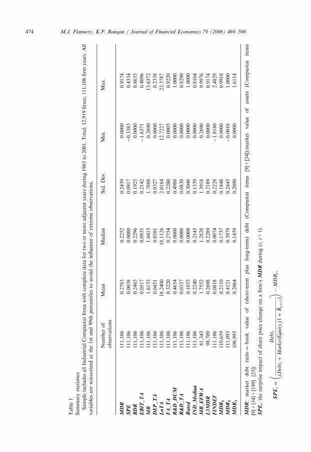
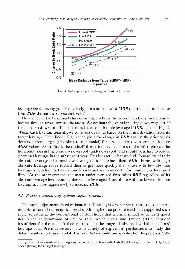
We construct our sample from all firms included in the Compustat Industrial Annualtapes between the years 1965 and 2001. Following previous research, we exclude financialfirms (SIC 6000–6999) and regulated utilities (SIC 4900–4999), whose capital decisionsmay reflect special factors. Because our regression specification includes lagged variables,we must also exclude any firm with fewer than two consecutive years of data. Theseexclusions leave us with complete information for 111,106 firm-year observations, whichconsist of 12,919 firms with an average of 9.6 years each.3 Some prior studies excludesmaller firms from the analysis, because their adjustment costs may be unusually large ortheir leverage determinants might be significantly different. We include all firms in ourestimations, but Table 9 reports estimates of the main regression model for various firmsize classes. We define annual observations on the basis of fiscal (as opposed to calendar)years because sample firms use a variety of fiscal yearends. Table 1 defines the variablesused in our study and reports their summary statistics. All of these variables are winsorizedat the 1st and 99th percentiles to avoid the influence of extreme observations. Most of ourvariables are expressed as ratios; where this is not the case (e.g. LnTA), we deflate thenominal magnitudes by the consumer price index to express nominal values in 1983dollars.To model a target debt ratio, we use a set of firm characteristics (Xi,t) that appear
regularly in the literature (Rajan and Zingales, 1995; Hovakimian, 2003; Hovakimian etal., 2001; Fama and French, 2002). Their expected effects on the target debt ratio are asfollows:
EBIT_TA: A firm with higher earnings per asset dollar could prefer to operate witheither lower or higher leverage. Lower leverage might occur as higher retained earningsmechanically reduce leverage, or if the firm limits leverage to protect the ‘‘franchise’’producing these high earnings. Higher leverage might reflect the firm’s ability to meetdebt payments out of its relatively high cash flow.MB: Market to book ratio of assets. A higher MB is generally taken as a sign of moreattractive future growth options, which a firm tends to protect by limiting its leverage.DEP_TA: Depreciation as a proportion of total assets. Firms with more depreciationexpenses have less need for the interest deductions provided by debt financing.LnTA: Log of (real) total assets. Larger firms tend to operate with more leverage,perhaps because they are more transparent, have lower asset volatility, or have betteraccess to public debt markets.FA_TA: Fixed asset proportion. Firms operating with greater tangible assets have ahigher debt capacity.R&D_TA: Research and development expenses as a proportion of total assets. Firmswith more intangible assets in the form of R&D expenses will prefer to have moreequity.
3The minimum number of years per firm is two, the maximum is 37, and the median is six. In the parlance of
panel data analysis, this constitutes a ‘‘large N, small T’’ data set.

ARTICLE IN PRESS
4
yie
Ta
M.J. Flannery, K.P. Rangan / Journal of Financial Economics 79 (2006) 469–506 477
R&D_DUM: A dummy variable equal to one for firms with missing R&D expenses.About 55% of our sample firm-years do not report R&D expenses. For these firms, weset R&D expense to zero and set R&D_DUM equal to one.Ind_median: The firm’s lagged industry median debt ratio (using Fama and French,1997 industry definitions), to control for industry characteristics not captured by otherexplanatory variables. (See also Hovakimian et al., 2001; Roberts, 2002).
In addition to these ‘‘usual’’ determinants of target leverage, we include firm-specificunobserved effects (li) to capture the impact of intertemporally constant, but unmeasured,effects on each firm’s target leverage. We find that these unobserved effects explain a largeproportion of the cross-sectional variation in target debt ratios, without displacing theother firm characteristics in Xi,t. At the same time, however, firm fixed effects complicatethe estimation problem by making the regression (4) a dynamic panel model (Bond, 2002).We discuss some of these econometric issues in the next section, and provide further detailsin the appendix.
4. Partial adjustment and the tradeoff theory
4.1. Appropriate estimation techniques
The first column in Table 2 presents Fama and MacBeth (1973) (FM) estimates of (4).4
Most of the lagged variables representing the target debt ratio carry significant coefficientswith appropriate signs. (Only MB and LnTA have insignificant coefficients.) Thecoefficient on lagged MDR implies that firms close 13.3% ( ¼ 1–0.867) of the gap betweencurrent and desired leverage within one year. At this rate, it takes approximately five yearsto close half the gap between a typical firm’s current and desired leverage ratios. This slowadjustment is consistent with the hypothesis that other considerations—e.g., pecking orderor market timing – outweigh the cost of deviating from optimal leverage. With such a lowestimated adjustment speed, convergence toward a long-run target seems unlikely toexplain much of the variation in firms’ debt ratios.
While the FM estimates have some attractive features, they fail to recognize the data’spanel characteristics. A panel regression with unobserved (fixed) effects is moreappropriate if firms have relatively stable, unobserved variables affecting their leveragetargets. Column (2) of Table 2 reports a fixed effects panel regression, whose estimatedcoefficients on the determinants of target leverage generally resemble their FM counter-parts, except for LnTA. The statistical significance of most variables is greater, and thefixed effects on target MDR are well justified: an F-test for the joint significance of theunobserved effects in column (2) rejects the hypothesis that these terms are equal across allfirms (F(12918, 98178) ¼ 2.24; pr ¼ 0.000). A prominent difference between columns (1)and (2) are the estimated coefficients on lagged MDR, which indicate a substantially fasteradjustment speed (38%) in the panel model. This estimated adjustment speed implies thatthe typical firm closes half of a leverage gap in about 18 months.
Fama and French (2002) recommend FM estimators to avoid understating coefficient standard errors. OLS
lds similar coefficient estimates for similar specifications, as shown in column (2) of Table 3 or column (2) of
ble A.1 in the appendix.
ARTICLE IN PRESS
Table 2
Alternate estimation methods for specification (4)
Regression results for the model
MDRi;tþ1 ¼ ðkbÞX i;t þ ði � kÞMDRi;1 þ di;tþ1; (4)
where MDR is the market debt ratio. The (lagged) ‘‘X’’ variables determine a firm’s long-run target debt ratio,
and include:
EBIT_TA: earnings before interest and taxes as a proportion of total assets;
MB: the market-to-book ratio of firm assets;
DEP_TA: depreciation expense as a proportion of total assets;
LnTA: natural log of total assets;
FA-TA: fixed assets as a proportion of total assets;
R&D_DUM: dummy variable indicating that the firm did not report R&D expenses;
R&D_TA: R&D expenses as a proportion of total assets;
Ind_Median: median debt ratio of firm i’s Fama and French (2002) industry classification at time t; and
Rated: dummy variable equal to one if the firm has a public debt rating in Compustat, zero otherwise.
Models (2) and (4)–(7) include firm fixed effects and models (4)–(7) include year dummies. T-statistics are shown
in parentheses. Reported R2 numbers for models including fixed effects are ‘‘within’’ R2 statistics.
(1) (2) (3) (4) (5) (6) (7)
FM FE panel FM
Demeaned
FE Panel
(with year
dummy)
IV panel IV panel,
Middle 50th
percentile
‘‘Base’’
specification
MDRi,t 0.867 0.620 0.639 0.620 0.656 0.636 0.656
(67.01) (218.03) (53.63) (225.14) (172.42) (67.19) (171.58)
EBIT_TA �0.035 �0.037 �0.051 �0.039 �0.030 �0.039 �0.030
(�3.97) (�11.80) (�4.70) (�12.96) (�9.64) (�7.64) (�9.66)
MB �0.001 0.000 �0.001 �0.001 0.000 0.002 0.000
(�1.53) (�0.34) (�1.45) (�3.38) (�0.68) (2.71) (�0.81)
DEP_TA �0.225 �0.280 �0.338 �0.224 �0.226 �0.209 �0.226
(�7.59) (�13.46) (�7.67) (�10.97) (�11.07) (�6.61) (�11.06)
LnTA 0.000 0.026 0.025 0.027 0.026 0.034 0.025
(�0.43) (38.22) (14.42) (37.52) (34.56) (30.28) (34.00)
FA_TA 0.022 0.058 0.066 0.059 0.053 0.058 0.053
(2.68) (12.82) (10.33) (13.42) (11.85) (8.33) (11.93)
R&D_DUM 0.005 �0.006 0.000 0.000 0.000 0.001 0.000
(3.97) (�3.87) (0.23) (�0.14) (�0.01) (0.35) (0.02)
R&D_TA �0.081 �0.038 �0.072 �0.036 �0.025 �0.074 �0.025
(�3.56) (�3.80) (�3.10) (�3.63) (�2.55) (�4.09) (�2.57)
Ind_Median 0.063 0.054 0.087 0.050 0.034 0.028 0.034
(5.71) (9.89) (4.43) (6.34) (4.29) (2.42) (4.30)
Rated 0.003
(1.71)
Fixed
effects?
No Yes No Yes Yes Yes Yes
N 111,106 111,106 111,106 111,106 111,106 55,526 111,106
R2 0.756 0.426 0.462 0.467 0.466 0.330 0.466
M.J. Flannery, K.P. Rangan / Journal of Financial Economics 79 (2006) 469–506478
The more rapid adjustment speed in column (2) might reflect either the addition of firmfixed effects to the target specification, or the panel regression constraint that the slopecoefficients remain constant over time. To distinguish between these two possibilities, theregression in column (3) applies the FM method to de-meaned data. That is, each variableis expressed as a deviation from that firm’s mean value. Most of the FM estimates in

ARTICLE IN PRESSM.J. Flannery, K.P. Rangan / Journal of Financial Economics 79 (2006) 469–506 479
column (3) are very close to the panel results in column (2). We conclude that firm-specificunobserved effects substantially influence estimated adjustment speeds, apparently becausethey substantially sharpen estimates of the target debt ratio.5 We return to this issue inSection 4.3.
Column (4) estimates a revised panel model, which includes a separate dummy variablefor each year in the sample (except 1966, to avoid a dummy variable trap). The resulting(within) adjusted-R2 statistic rises slightly from column (2) and the other coefficientsremain essentially the same. We include year dummy variables in our subsequent panelregressions to absorb any unmodeled time-varying influences on capital structure. We alsoestimate this specification with a correction for first-order serial correlation within eachpanel (not reported). The estimated AR(1) coefficient is sufficiently small (�0.03) that weproceed under the assumption that serial correlation is not a significant effect in our study.
Consistently estimating the adjustment speed in a dynamic panel requires careful attentionto the serial correlation properties of the dependent variable and the regression’s residuals(Baltagi, 2001, Chapter 8; Wooldridge, 2002). Column (5) addresses the correlation betweena panel’s lagged dependent variable and the error term, which can bias the estimatedadjustment speed. We substitute a fitted value for the lagged dependent variable, using thelagged book value of leverage and Xt as instruments (Greene, 2003).6 The estimated MDRt
coefficient rises slightly (from 0.620 to 0.656) but the other coefficient estimates remain closeto the estimates in column (4). The implied adjustment speed of 34.4% indicates that thetypical firm completes more than half of its required leverage adjustment in less than twoyears—far faster than estimated by many previous authors. Such a rapid adjustment towarda firm-specific capital ratio suggests that pecking order or market timing does not dominatemost firms’ debt ratio decisions. We return to this issue in Table 4 below.
Column (6) of Table 2 addresses the possibility that the rapid adjustment speed incolumn (5) reflects the bounded nature of MDRi,t between zero and unity. A firm with avery high leverage thus has nowhere to go but down, and vice versa. Column (6) reportsthe results of estimating our instrumental variables specification for only the middle 50%of observed MDRi,t values. The 25th and 75th percentile cutoffs for MDRi,t vary acrossyears, but average 6.5% and 41.6%, respectively. All of the coefficient estimates in column(6), including the adjustment speed, are very similar to the results using the entire sample.We are therefore confident that ‘‘hard-wired’’ mean reversion in the dependent variable isnot the cause of our high estimated adjustment speeds.
The last column of Table 2 presents our ‘‘base’’ specification that is used going forward.This specification includes an instrumental variable correction for MDRt. Explanatoryvariables include firm and time fixed effects, plus an additional explanatory variable in the‘‘X’’ matrix:
5Wh
in Fam
firm fi6Mo
some c7Bec
compa
Rated equals unity when a firm has a public debt rating, and zero otherwise.7
en we replace the firm fixed effects in column (2) with a set of 46 industry dummy variables (constructed as
a and French, 1997), the estimated coefficients closely resemble those in column (1), which also excludes
xed effects.
re recent estimation techniques like that of Arellano and Bond (1991) improve upon this approach under
ircumstances, but not for our sample. See the appendix for details.
ause Compustat does not report this variable before 1981, we cannot compute Fama–MacBeth estimates
rable to the other specifications in Table 2 if Rated is included.

ARTICLE IN PRESSM.J. Flannery, K.P. Rangan / Journal of Financial Economics 79 (2006) 469–506480
Faulkender and Petersen (2005) control for sample selectivity in their paperbecause Rated may be endogenous. We simply include Rated as an additionaldependent variable, for two reasons. First, the impact of bond ratings is not ourcentral concern. Second, the other results are completely insensitive to the inclusion orexclusion of Rated from the set of variables determining a firm’s target debt ratio. Thisdummy variable carries a marginally significant positive coefficient (as in Faulkender andPetersen, 2005), but its introduction has no meaningful effect on the other coefficientestimates.Our base specification in column (7) indicates that the typical firm’s target debt ratio
varies quite a lot. The cross-sectional mean target debt ratio starts at 32.1% in 1966, risesto a maximum of 64.0% in 1974, and ends the period at 27.0% in 2001. Over the entiresample, the estimated target has an average of 30.7% and a standard deviation of 25.1%.(In comparison, the actual MDR’s mean and standard deviation are 27.8% and 24.4%,respectively.) Firm characteristics, fixed effects, and time all contribute to the variation intarget debt ratios. The set of nine X variables explain 16.0% of the total sample standarddeviation of MDR, the unobserved (fixed) effects explain 25.2%, and the year dummiesexplain 9.0%. Within each year, the nine X variables alone explain between 12.5% and17.6% of the annual, cross-sectional variations in target debt ratios, with an average(across all years) of 15.03%. In short, our computed leverage targets vary substantiallyacross firms and across time.
4.2. Convergence toward the target
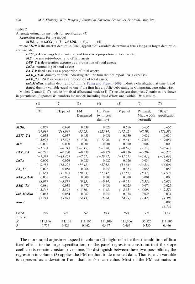
If we estimate meaningful leverage targets, we should find that firms adjust toward thesetargets over time. Fig. 1 illustrates managers’ financing decisions conditional on the firm’sdeviation from its computed (estimated) target leverage. For each year between 1966 and2000, we sort firms into quartiles on the basis of their deviations from target leverage(MDR�–MDR). The horizontal axis in Fig. 1 indicates that the firms in Quartile 1 appearto be substantially overleveraged, by an average (median) of 15.29% (13.59%) of assets.Conversely, our model indicates that the firms in Quartile 4 are underleveraged by a mean(median) of 21.96% (19.70%). The vertical axis in Fig. 1 describes the subsequent year’schange in book debt ratios (BDR), which should reflect the firm’s explicit efforts to movetoward its target. (In contrast, MDR confounds the effects of managerial actions andchanges in the firm’s stock price.) The evidence in Fig. 1 is consistent with convergence.The mean (median) overleveraged firm in Quartile 1 reduces its book leverage thefollowing year by 3.12% (1.94%). Conversely, the underleveraged firms in Quartile 4 raisetheir BDR by a mean (median) of 4.69% (1.75%) during the subsequent year. Firms in themiddle two quartiles also move toward their target debt ratios, but with much smalleradjustments.While the results in Fig. 1 are consistent with targeting behavior, they might reflect
merely a tendency of firms with relatively high or low debt ratios to move back toward themean, as indicated by Leary and Roberts’ (2005) hazard function estimates. Indeed, Fig. 2illustrates this tendency in the data. The horizontal axis describes four quartiles formed onthe basis of the prior year’s absolute MDR. As in Fig. 1, the vertical axis of Fig. 2 plots thesubsequent year’s mean and median changes in book debt ratio (BDR). Independent oftheir position relative to their target, highly levered firms tend to reduce their book
ARTICLE IN PRESS
-0.3%
0.7%
2.7%
6.8%
-4.1%
-1.6%
-0.3%
1.9%
-5%
-3%
-1%
1%
3%
5%
7%
Mean Distance from Target (MDR* - MDR)in year t-1
Ch
ang
e in
Bo
ok
Deb
t R
atio Lowest MDR
Low MDR
High MDR
Highest MDR
Fig. 3. Subsequent year’s change in book debt ratio.
M.J. Flannery, K.P. Rangan / Journal of Financial Economics 79 (2006) 469–506 481
leverage the following year. Conversely, firms in the lowest MDR quartile tend to increasetheir BDR during the subsequent year.8
How much of the targeting behavior in Fig. 1 reflects this general tendency for extremelylevered firms to revert toward the mean? We evaluate this question using a two-way sort ofthe data. First, we form four quartiles based on absolute leverage (MDRt�1) as in Fig. 2.Within each leverage quartile, we construct quartiles based on the firm’s deviation from itstarget leverage. Each line in Fig. 3 then plots the change in BDR against the prior year’sdeviation from target (according to our model) for a set of firms with similar absoluteMDR values. As in Fig. 1, the tradeoff theory implies that firms to the left (right) on thehorizontal axis in Fig. 3 are overleveraged (underleveraged) and should be acting to reduce(increase) leverage in the subsequent year. This is exactly what we find. Regardless of theirabsolute leverage, the most overleveraged firms reduce their BDR. Firms with highabsolute leverage move toward their target more quickly than those with low absoluteleverage, suggesting that deviations from target are more costly for more highly leveragedfirms. At the other extreme, the mean underleveraged firm raises BDR regardless of itsabsolute leverage level. Among these underleveraged firms, those with the lowest absoluteleverage act most aggressively to increase BDR.
4.3. Previous estimates of optimal capital structure
The rapid adjustment speed estimated in Table 2 (34.4% per year) constitutes the mostnotable feature of our empirical results. Although some prior research has supported suchrapid adjustment, the conventional wisdom holds that a firm’s annual adjustment speedlies in the neighborhood of 8% to 15%, which Fama and French (2002) considerinsufficient for the tradeoff theory to explain the range of observed variation in firms’leverage data. Previous research uses a variety of regression specifications to study thedeterminants of a firm’s capital structure. Why should our specification be preferred? We
8Fig. 2 is not inconsistent with targeting behavior, since firms with high (low) leverage are more likely to be
above (below) their target leverage.

ARTICLE IN PRESSM.J. Flannery, K.P. Rangan / Journal of Financial Economics 79 (2006) 469–506482
contend that most previous studies impose unwarranted, but testable, assumptions on thedata, which have led to incorrect or misleading inferences.Table 3 reports a set of capital structure models estimated over the same panel data set.
Column (1) presents a typical simple, cross-sectional specification used by many priorstudies to infer the determinants of a firm’s optimal leverage (e.g., Hovakamian et al.,(2001); Fama and French (2002); Korajczyk and Levy (2003); Kayhan and Titman(2005)).9 The estimated coefficients resemble those of the earlier studies. In particular,higher earnings, MB ratio, R&D expenditures, and depreciation expenses lower targetleverage, while asset size and fixed assets raise it.The specification in column (1) constrains the coefficient on lagged MDR to be zero. In
other words, a firm’s observed capital ratio is also its desired (target) ratio. Column (2)indicates that this hypothesis is strongly rejected by the data. When we add the laggeddependent variable to the specification in column (1), it carries a very highly significantcoefficient (0.864). The simple cross-sectional regression in column (1) thus appears to omitan important variable. We also know from Table 2 that column (2)’s exclusion of firm fixedeffects is unwarranted.Column (3) specifies partial adjustment toward a target capital ratio that includes firm
fixed effects.10 Several of the estimated coefficients differ substantially from those for thesimple linear model in column (1). For example, column (1) indicates that the coefficienton EBIT_TA is �0.282, more than three times the estimated long-run magnitude incolumn (3) ((�0.03/0.343) ¼ �0.087). The long-run coefficients on MB, R&D_Dum,R&D_TA, and Rated are also substantially lower in column (3), while the long-run impactof firm size (LnTA) increases by a factor of six. It appears, therefore, that the estimateddeterminants of target leverage are materially affected by the omitted variables in column(1).11
Regressions like that in column (1) are sometimes used to generate leverage targetproxies for use in partial adjustment models. Two-stage estimates based on such a proxyhave largely formed the conventional wisdom that firms adjust slowly toward any leveragetarget. Column (4) of Table 3 presents an estimated partial adjustment model based on atarget debt ratio (TDROLS,), which is computed from column (1). The estimatedadjustment speed (9.1%) resembles other estimates derived from target proxies containingno fixed effects. This alone does not indicate a problem with the two-stage estimation.However, the coefficient on TDROLS is much smaller than theory would predict. Thelongrun elasticity of observed MDR with respect to its target should be unity. Here, it isonly 0.56 ( ¼ 0.051/0.091), which differs from unity at a very high confidence level
9Hovakimian et al. (2001) and Korajczyk and Levy (2003) estimate a target leverage using simple OLS, then use
deviations from their computed targets to help predict whether a firm subsequently issues debt or equity.10This regression omits one determinant of the target debt ratio from our base specification, namely, the lagged
industry median MDR. We omit this variable in Table 3 in order to provide a cleaner test of the two-stage
approach to estimating a partial adjustment coefficient.11Hovakimian et al. (2004) estimate a cross-sectional regression like our column (1) for a set of firms that have
recently issued large amounts of both debt and equity, and find that the estimated coefficients differ substantially
from those estimated for the rest of the Compustat universe. The authors argue that the security issuers have
moved close to their optimal leverage ratios, while the other firms are scattered more widely relative to their target
capital ratios.

ARTICLE IN PRESS
Table 3
The importance of recognizing partial adjustment
Regression results for the models
(1) MDRi,t+1 ¼ b Xi,t+di,t+1,
(2) MDRi,t ¼ (k b) Xi,t+(1�k) MDRi,t+di,t+1,
(3) MDRi,t+1 ¼ (k b) Xi,t+(1�k) MDRi,t+ni+di,t+1,
(4) MDRi,t+1 ¼ k (TDROLS i)+(1�k1) MDRi,t+di,t+1,
(5) MDRi,t+1 ¼ b1 L3MDRi,t+(1�k1) MDRi,t+di,t+1,
where MDR is the market debt ratio. The (lagged) ‘‘X’’ variables determine a firm’s long-run target debt ratio,
and include:
EBIT_TA: earnings before interest and taxes as a proportion of total assets;
MB: the market-to-book ratio of firm assets;
DEP_TA: depreciation expense as a proportion of total assets;
LnTA: natural log of total assets;
FA-TA: fixed assets as a proportion of total assets;
R&D_DUM: dummy variable indicating that the firm did not report R&D expenses;
R&D_TA: R&D expenses as a proportion of total assets; and
Rated: dummy variable equal to one if the firm has a public debt rating in Compustat, and zero otherwise.
L3MDR is the average of the three-years’ lagging MDR values, and TDROLS is the fitted value from model
(1). All regressions include(unreported) year dummies. T-statistics are shown in parentheses. Reported R2
numbers for models including fixed effects are ‘‘within’’ R2 statistics.
(1) (2) (3) (4) (5)
MDRi,t 0.864 0.657 0.909 0.935
(469.79) (174.09) (382.34) (194.48)
EBIT_TA �0.282 �0.026 �0.030
(�75.25) (�11.62) (�9.73)
MB �0.041 �0.002 0.000
(�103.01) (�6.84) (�1.07)
DEP_TA �0.566 �0.216 �0.225
(�24.87) (�16.38) (�11.03)
LnTA 0.011 �0.001 0.025
(26.39) (�3.11) (33.85)
FA_TA 0.128 0.027 0.054
(36.32) (13.16) (12.19)
R&D_DUM 0.035 0.007 0.000
(24.33) (8.73) (0.03)
R&D_TA �0.518 �0.116 �0.026
(�50.79) (�19.51) (�2.64)
Rated 0.066 0.005 0.003
(26.45) (3.68) (1.75)
TDROLS 0.051
(12.31)
L3MDR �0.023
(�4.85)
Fixed effects? No No Yes No No
N 111,106 111,106 111,106 111,106 81,343
R2 0.262 0.753 0.466 0.750 0.767
M.J. Flannery, K.P. Rangan / Journal of Financial Economics 79 (2006) 469–506 483

ARTICLE IN PRESSM.J. Flannery, K.P. Rangan / Journal of Financial Economics 79 (2006) 469–506484
(t ¼ 11.48).12 This provides strong evidence against the two-step estimation procedureused previously in the literature.Target leverage has also been proxied by the trailing average of a firm’s actual
leverage.13 In column (5), we test whether L3MDR, a three-year trailing average MDR,provides an adequate proxy for target capital. The estimated adjustment speed is now only6.5%, and the impact of a one-unit increase in L3MDR actually reduces a firm’s longrundebt ratio. Thus, it appears that L3MDR measures target leverage quite poorly.We now investigate more formally how target measurement noise affects a partial
adjustment model. Could measurement error alone account for the difference between theadjustment speeds in columns (2) and (3) of Table 3? Substitute a noisy proxy for MDR�
into Eq. (3) to obtain
MDRi;tþ1 ¼ ð1� kÞMDRi;t þ kðMDR�i;tþ1 þ~ni;tÞ þ
~di;tþ1, (3a)
where ~xi;t is a standard normal variate with zero mean. Adding noise to an explanatoryvariable usually biases the associated coefficient toward zero, which implies an estimatedcoefficient on MDRi,t biased toward unity. To quantify this effect, we assume thatMDR� ¼ TDRPanel, a target series constructed from the estimated coefficients in column(3) of Table 3. We then increase the standard deviation of ~xi;t from 0.0 to 0.5 across thecolumns of Table 4.14 The results indicate that a noisier target measure lowers both theestimated adjustment speed (from 0.345 to 0.104) and the long-run effect on MDR of achange in the target’s value (from 1.00 to 0.31).Which column of Table 4 is most relevant for our data set? Over the entire sample
period, the observed MDR series has a standard deviation of 24.4%. A good proxy shouldbe similarly distributed and TDRPanel has a standard deviation of 25.1%. In contrast, theTDROLS series’ standard deviation is much smaller (12.5%). The standard deviation of thedifference between these two target proxies (TDRPanel–TDROLS) is about 22%, which liesbetween the assumed noise volatilities in columns (4) and (5) of Table 4. We therefore seethat a noise volatility of 20% to 25% roughly halves the estimated adjustment speed; from34.5% (E1–0.656) to something in the neighborhood of 17%.15
We conclude from Tables 3 and 4 that partial adjustment and firm fixed effects should beincluded in a model of firm capital structure choice. A few previous studies include such
12The importance of fixed effects in computing leverage targets can be assessed by reestimating the regression in
column (1) with firm fixed effects. When the resulting fitted values are used as leverage targets, the adjustment
speed in column (4) rises to 40% and its long-run impact on MDR is 1.05.13Marsh (1982); Jalilvand and Harris (1984); and Shyam-Sunder and Myers (1999) have used various forms of
this proxy, with mixed results. In Section 5.3 below, we point out that Welch’s (2004) main regression specification
can be viewed as a single lag of the dependent variable as a leverage target.14The TDRPanel series is itself a noisy estimate of the true target, so ~xi;t measures additional ‘‘noise,’’ not the
total estimation error.15Further qualitative evidence that measurement error depresses estimated adjustment speeds comes from
comparing various versions of Kayhan and Titman (2005). Although their focus is quite different from ours, they
estimate a regression of the form
MDRt �MDRt�k ¼ aX þ bðMDRt�k � TDRt�kÞ þ et, (6)
where TDRt– k is the target debt ratio computed from a cross-sectional OLS regression using firm characteristics
from year (t�k�1). When k ¼ 5 (as it does in Table 6 of their November 2003 manuscript), b ¼ 0:45, whichimplies an annual leverage adjustment rate of 7.7%. In the corresponding table of their May 2004 revision, they
set k ¼ 10 and the estimated annual adjustment speed falls to 4.6%. Although this change has no effect on their
variables of interest, it does illustrate the effect of noisy targets on the estimated adjustment speed.

ARTICLE IN PRESS
Table 4
Effect of Adding Noise to the Target Debt Ratio
Regression results for the model
MDRi;tþ1 ¼ ð1� kÞMDRi;t þ kðMDR�i;tþ1 þ~ni;tÞ þ
~di;tþ1: (3a)
where MDR is the market debt ratio, MDR* is the estimated target debt ratio from model (3) of Table 3, and ~ni;t
is a white noise term with zero mean. Models (1) through (6) are estimated at various levels of standard deviation
for ~ni;t. T-statistics are shown in parentheses.
(1) (2) (3) (4) (5) (6)
Standard deviation of ~ni;t0% 5% 10% 20% 25% 50%
MDRt 0.656 0.680 0.731 0.818 0.844 0.896
(230.82) (246.07) (278.24) (345.06) (370.89) (432.96)
MDR�i;tþ1 þ ~xi;t 0.345 0.313 0.248 0.130 0.100 0.033
(145.05) (138.98) (123.97) (90.45) (78.10) (46.19)
N 111,106 111,106 111,106 111,106 111,106 111,106
R2 0.811 0.806 0.795 0.774 0.768 0.755
Long-run effect of target 1.000 0.979��� 0.920��� 0.729��� 0.632��� 0.312���
���Significantly different from one at the 1% level.
M.J. Flannery, K.P. Rangan / Journal of Financial Economics 79 (2006) 469–506 485
features in their regression models and produce rapid estimated adjustment speeds. Forexample, Marcus (1983) estimates a panel model with firm fixed effects for large U.S.banks over the period 1965–1977. His estimated adjustment speed for market leverage is20–24% per year for the full sample. For the 1965–1971 subperiod, he estimates annualadjustment speeds as high as 32.5%. Roberts (2002) estimates even higher adjustmentspeeds in his Kalman filter model of partial adjustment. Because the standard Kalmanfilter specifies that all variables have zero means, he de-means each data series, which‘‘implicitlyyaccounts for firm-specific effects in the intercepts’’ (p. 13). Using quarterlydata over the period 1980–1998, he estimates a separate model similar to Eq. (4) for thefirms in each of 53 industries. His results imply annual adjustment speeds (l) ranging froma low of 18% to a high of more than 100%.16
In a multifaceted paper, Leary and Roberts (2005) use a quarterly Compustat data set(1984–2001) to estimate hazard functions for substantial net debt or equity adjustments.17
While their primary concern is to infer the form of capital adjustment costs (e.g., fixed vs.proportional vs. convex), but they indirectly address the question of adjustment speeds.They find that a typical firm changes the book value of its debt (equity) by more than 5%of book assets about once per year, and conclude that ‘‘Firms do indeed respond to equityissuances and equity price shocks by appropriately rebalancing their leverage over the nextone to four years’’ (p. 32). If we define ‘‘appropriately rebalancing’’ as closing 90% of theinitial leverage gap, ‘‘one to four years’’ corresponds to an adjustment speed in Eq. (4) thatexceeds 40%.
16Across all industries, the mean annual adjustment speed is approximately is 43%. His equal-weighted average
of 53 industries’ adjustment speeds cannot be compared directly to our estimated l. We weight each sample firm
equally, which gives different industries different weights in our estimate of l. Still, it is comforting to learn that
applying Kalman filters to a comparable data set yields roughly similar results.17They describe the estimated model as ‘‘similar in spirit to a nonlinear dynamic panel regression with firm-
specific random effects’’ (p. 17, emphasis added).

ARTICLE IN PRESSM.J. Flannery, K.P. Rangan / Journal of Financial Economics 79 (2006) 469–506486
Alti (2004) estimates relatively rapid adjustment speeds without fixed effects in his targetvariable specification. He compares the capital ratios chosen by 1,363 firms that go publicin ‘‘hot’’ vs. ‘‘cold’’ issue markets. He finds that firms making their IPOs in a hot (cold)market tend to have unusually low (high) leverage immediately after going public. He thenestimates a model similar to Eq. (4), but without fixed effects, for one and two years afterthe IPO date. The estimated adjustment speed is surprisingly rapid for a model withoutfixed effects: 30% per year. We conjecture that this rapid adjustment reflects his sample:rapidly growing, young firms tend to seek additional financing soon after their IPO andhence confront unusually low costs of adjusting leverage.In conclusion, our model specification is theoretically preferable to many earlier models,
and the specification differences account for our main results: firms adjust rapidly towardtime-varying target leverage ratios, which depend on plausible firm features.
5. Other capital structure theories
The pecking order model has strong intuitive appeal and a long pedigree. Various formsof the model have been recently studied, with mixed empirical results (Shyam-Sunder andMyers, 1999; Frank and Goyal, 2003; Lemmon and Zender, 2004; Halov and Heider,2004). The literature also includes two more recent explanations of capital structure,namely, Baker and Wurgler’s (2002) market timing theory (also studied in Huang andRitter, 2005) and Welch’s (2004) mechanical stock price explanation. We now compare ourresults to these three alternatives.
5.1. The pecking order and market timing theories: regression evidence
Previous authors estimate models in which the financing deficit (pecking order) or theweighted sum of past market-to-book ratios (market timing) compete with variablesassociated with the tradeoff theory of capital structure. The idea is that the variablesassociated with the ‘‘true’’ theory are more important than their competitors. Frank andGoyal (2003) explain:
18Th
well as
The pecking order theory implies that the financing deficit ought to wipe out theeffects of other variables. If the financing deficit is simply one factor among manythat firms tradeoff, then what is left is a generalized version of the tradeoff theory.(p. 219)
Baker and Wurgler (2002) make similar statements, particularly concerning theirTable III.Pecking order behavior implies that a firm’s financing deficit explains contemporaneous
changes in its book debt ratio. We test this proposition by evaluating a book-value analogto our main specification in Eq. (4):18
DBDRi;tþ1 ¼ ðkbÞX i;t � kBDRi;t þ c2FINDEF i;tþ1 þ ei;tþ1, (7)
where BDR is the ratio of (long-term plus short-term debt) to total assets, and FINDEF isthe firm’s financing deficit. In their Table 2, Frank and Goyal (2003) define FINDEF as:
e bias associated with including the lagged dependent variable in a panel regression applies to (7) and (8) as
it does to (4). In these cases, we instrument for lagged BDR using the firm’s lagged MDR.

ARTICLE IN PRESSM.J. Flannery, K.P. Rangan / Journal of Financial Economics 79 (2006) 469–506 487
(dividend payments+investments+change in working capital�internal cashflow)/(totalassets).
Baker and Wurgler (2002) assert that managers issue relatively overvalued securities,which can be either debt (when the firm’s q-ratio is low) or equity (when q is high). Theyconstruct a backward-looking ‘‘external finance weighted average’’ book-market ratio,which they find to be correlated with a firm’s book debt ratio over periods as long as tenyears. We test their hypothesis here by estimating the following regression for the level ofBDR:
BDRi;tþ1 ¼ ðkbÞX i;t � ð1� kÞBDRi;t þ c1MB_EFWAi;t þ ei;tþ1, (8)
where MB_EFWA is the firm’s external finance weighted average book-market ratiodefined on 12 of Baker and Wurgler (2002).
In both regressions (7) and (8), the question is whether MB_EFWA or FINDEF affectsthe estimated coefficients on Xi,t or the lagged dependent variable. To set a baseline for theBDR regressions, the first column in Table 5 reports the results of explaining BDR withonly our standard Xi,t (including firm fixed effects), year dummies, and a lagged dependentvariable. The partial adjustment model fits BDR well: the lagged dependent variable’scoefficient implies a rapid adjustment (36.1% annually) and the variables meant to capturetarget leverage carry significant coefficients with the appropriate signs. Adding Baker andWurgler’s (2002) external finance weighted market-book ratio as an explanatory variablein column (2) lowers the estimated adjustment speed only slightly (from 36.1% to 34.2%).The other coefficients remain basically unchanged, except that the simple MB coefficientloses significance. The Baker and Wurgler (2002) variable is at best marginally significant(p-value ¼ 0.093, two-tailed test), perhaps because the market-to-book effect is splitbetween the two variables (Hovakimian, 2003).
The specification in column (3) explains the change in BDR with changes in our standardexplanatory variables and the firm’s financing deficit. The FINDEF coefficient issignificantly positive (t-statistic ¼ 9.96), but does not substantially alter the othervariables’ signs and significance levels. Thus, the pecking order forces appear to be partof a ‘‘generalized version of the tradeoff theory’’ (Frank and Goyal, 2003, p. 219), ratherthan a unique determinant of financial leverage.
We next include both MB_EFWA and FINDEF in the same regression. This is probablyan inappropriate specification because MB_EFWA is meant to explain the level of BDRwhile FINDEF affects the change in BDR. Nevertheless, the estimated coefficients incolumn (4) resemble their values in columns (2) and (3), and the tradeoff variables retaintheir usual values.
Although both the pecking order and market timing hypotheses apply to book-valueddebt ratios, columns (5)–(7) of Table 5 incorporate MB_EFWA and FINDEF intoregressions explaining the market debt ratio. The market-timing variable (MB_EFWA) incolumn (5) now carries a significant coefficient with the proper sign. As in column (2), thesimple MB variable again loses significance. The pecking order conclusions in column (6)replicate those for DBDR in column (3): FINDEF carries a significantly positive coefficientbut does not displace the tradeoff-related variables from the regression. Once again,including both of the competing theories’ variables in column (7) yields significantcoefficients without substantially changing the estimated coefficients on the tradeoff orpartial adjustment variables.

ARTICLE IN PRESS
Table
5
Peckingorder
andmarket
timingexplanationsofbookdebtratio
Incolumns(1)(2),and(4),weestimate
aregressionthatexplainsafirm
’sbookdebtratio:
BD
Ri;
tþ1¼ðlbÞ
Xi;
tþð1�
lÞB
DR
i;tþ
g 1Z
i;tþ
e i;tþ
1.
Incolumn(4),weestimate
aregressionthatexplainsafirm
’schangein
bookdebtratio:
DB
DR
i;tþ
1¼ðlbÞ
Xi;
t�
lBD
Ri;
tþ
g 2Z
i;tþ
e i;tþ
1,
Incolumns(5)and(7)weestimate
ourmain
regressionspecificationthatexplainsafirm
’smarket
debtratio:
MD
Ri;
tþ1¼ðlbÞ
Xi;
t�ð1�
lÞM
DR
i;tþ
c 1Z
i;tþ
d i;tþ1:
(4)
Incolumn(6)weestimate
aregressionthatexplainsafirm
’schangein
market
debtratio:
DM
DR
i;tþ
1¼ðlbÞ
Xi;
t�
lMD
Ri;
tþ
g 2Z
i;tþ
d i;tþ1.
The(lagged)‘‘
X’’variablesdetermineafirm
’slong-runtarget
debtratio,andinclude:
EB
IT_
TA:earningsbefore
interest
andtaxes
asaproportionoftotalassets;
MB:themarket-to-bookratiooffirm
assets;
DE
P_T
A:depreciationexpense
asaproportionoftotalassets;
Ln
TA:naturallogoftotalassets;
FA
-TA:fixed
assetsasaproportionoftotalassets;
R&
D_D
UM:dummyvariable
indicatingthatthefirm
did
notreport
R&D
expenses;
R&
D_
TA:R&D
expensesasaproportionoftotalassets;
Ind
_M
edia
n:mediandebtratiooffirm
i’sFamaandFrench
(2002)industry
classificationattime
t;and
Ra
ted:
dummyvariable
equalto
oneifthefirm
hasapublicdebtratingin
Compustat,andzero
otherwise.
Ztare
additionalexplanatory
variablesandinclude:
FIN
DE
F¼
ameasure
ofthefirm
’sfinancialdeficit,defined
asdividendpayments+
investments+
changein
workingcapital�
internalcashflow;or
MB
_E
FW
A¼
an‘‘externalfinance
weightedaverage’’market-bookratiodefined
byBaker
andWurgler(2002,p.12).
Allmodelsinclude(unreported)yeardummies.
T-statisticsare
shownin
parentheses.Reported
R2numbersformodelsincludingfixed
effectsare
‘‘within’’
R2
statistics.
M.J. Flannery, K.P. Rangan / Journal of Financial Economics 79 (2006) 469–506488

ARTICLE IN PRESS
Pan
elA
:E
stim
ati
on
resu
lts
(1)
(2)
(3)
(4)
(5)
(6)
(7)
DependentVariable
BD
RBDR
DB
DR
BD
RMDR
DM
DR
MDR
BD
Ri,
t0.639
0.658
�0.375
0.645
(1
67.2
1)
(1
66.4
2)
(�
90
.32
)(
15
0.2
2)
MD
Ri,
t0.670
�0.341
0.645
(1
63
.84
)(�
86
.53)
(1
46
.10
)
EB
IT_
TA
�0.024
�0.026
�0.018
�0.019
�0.030
�0.021
�0.020
(�
9.4
8)
(�
8.5
7)
(�
6.6
1)
(�
5.8
9)
(�
7.7
0)
(�
6.6
3)
(�
4.6
9)
MB
�0.001
0.000
�0.001
�0.001
0.001
�0.001
�0.001
(�
2.8
8)
(�
0.0
7)
(�
4.9
0)
(�
2.0
6)
(1
.53
)(�
2.2
0)
(�
1.5
4)
DE
P_
TA
�0.194
�0.191
�0.144
�0.152
�0.275
�0.155
�0.205
(�
11
.32)
(�
10
.01)
(�
7.6
7)
(�
7.2
8)
(�
11
.35
)(�
7.3
3)
(�
7.7
9)
LnT
A0.008
0.009
0.008
0.008
0.026
0.026
0.026
(1
3.4
2)
(1
3.3
6)
(1
2.2
2)
(1
1.1
3)
(3
1.2
7)
(3
3.1
2)
(2
8.3
0)
FA
_TA
0.042
0.041
0.041
0.038
0.052
0.057
0.056
(1
1.1
7)
(1
0.1
5)
(9
.92
)(
8.5
9)
(1
0.3
6)
(1
2.2
4)
(1
0.1
4)
R&
D_
DU
M�0.001
�0.001
�0.001
�0.001
�0.001
0.001
0.001
(�
0.7
9)
(�
1.0
1)
(�
0.7
5)
(�
0.7
7)
(�
0.3
3)
(0
.48)
(0
.40
)
R&
D_
TA
�0.026
�0.021
�0.019
�0.013
�0.033
�0.010
�0.015
(�
3.1
8)
(�
1.8
5)
(�
2.1
8)
(�
1.0
8)
(�
2.3
1)
(�
1.0
8)
(�
1.0
4)
Ra
ted
0.008
0.006
0.008
0.007
0.001
0.003
0.003
(5
.28)
(4
.24)
(4
.97
)(
4.2
5)
(0
.53
)(
1.7
7)
(1
.35
)
IND
_Med
ian
0.032
0.030
0.032
0.031
0.031
0.030
0.037
(4
.93)
(4
.66)
(4
.47
)(
4.3
9)
(3
.77
)(
3.6
8)
(4
.09
)
MB
_EF
WA
�0.001
�0.001
�0.003
�0.004
(�
1.6
8)
(�
1.1
9)
(�
4.5
4)
(�
4.9
9)
FIN
DE
F0.021
0.028
0.023
0.048
(9
.96
)(
9.8
2)
(9
.71)
(1
3.3
1)
Fixed
effects?
Yes
Yes
Yes
Yes
Yes
Yes
Yes
N111,106
94,235
98,709
83,790
94,235
98,709
83,790
R2
0.384
0.420
0.198
0.398
0.475
0.240
0.443
M.J. Flannery, K.P. Rangan / Journal of Financial Economics 79 (2006) 469–506 489

ARTICLE IN PRESS
Pa
nel
B:
Rel
ati
veec
on
om
icsi
gn
ifica
nce
of
capit
al
stru
ctu
reth
eori
es
Column(2)ofPanel
AColumn(3)ofPanel
AColumn(5)ofPanel
AColumn(6)ofPanel
A
Impact
on
BD
RIm
pact
on
DB
DR
Impact
on
MD
RIm
pact
on
DM
DR
Absolute
%of
BD
R’s
Std.Dev.
Absolute
%ofD
BD
R’s
Std.Dev.
Absolute
%of
MD
R’s
Std.Dev.
Absolute
%ofD
MD
R’s
Std.Dev.
Tradeoff
Theory
Estim
ated
Target
0.0617
32.94%
0.0711
65.49%
0.0676
27.82%
0.0748
60.14%
Market
Tim
ing
Theory
MB
_E
FW
A�0.0014�0.73%
NA
NA
�0.007
�2.88%
NA
NA
PeckingOrder
Theory
FIN
DE
FNA
NA
0.0047
4.31%
NA
NA
0.0022
1.77%
Table
5(c
onti
nu
ed)
M.J. Flannery, K.P. Rangan / Journal of Financial Economics 79 (2006) 469–506490

ARTICLE IN PRESSM.J. Flannery, K.P. Rangan / Journal of Financial Economics 79 (2006) 469–506 491
Panel B of Table 5 assesses the economic significance of the tradeoff, market timing, andpecking order models by comparing their ability to explain variations in BDR and MDR.The first row in Panel B applies the coefficients from column (2) of Panel A. We calculatethat changing the target leverage (BDR�) by one standard deviation changes the (short-run) fitted BDR by 0.0617, which is about one-third of its standard deviation (0.1925). Incontrast, changing MB_EFWA by one standard deviation lowers BDR by 0.0014 (less than1% of its standard deviation). Using coefficient estimates from column (3) of Panel A, aone-standard deviation change in BDR� changes DBDR by 0.0711, while a similar changein FINDEF affects DBDR by only 0.0047. It therefore appears that variation in targetleverage is much more important than mispricing or a financing deficit in explaining bookdebt ratios. Similar assessments of the three capital structure theories emerge from the lasttwo columns in Panel B, which are based on the regressions in columns (5) and (6) of PanelA. Once again, the target leverage ratio explains far more of the variation in market debtratios than either the market timing or the pecking order variables.
Although the pecking order and market timing theories each add some information tothe regressions, we conclude that neither can replace our model of partial adjustmenttoward a target debt ratio. Targeting behavior consistent with the tradeoff theory seems toexplain the bulk of the observed capital structure.
5.2. Targeting leverage vs. stockpiling debt capacity
Lemmon and Zender (2004) (LZ) suggest a modified version of the pecking order theory,in which each firm has a ‘‘debt capacity,’’ or maximum attainable leverage. Empirically,their debt capacity depends on a set of firm characteristics that overlap somewhat with ourdeterminants of target leverage. As we do in Fig. 1, LZ classify a firm as ‘‘underleveraged’’or ‘‘highly leveraged’’ relative to its estimated debt capacity. They argue that overleveragedfirms have no choice but to reduce leverage because they cannot borrow further in themarket. However, LZ observe that the tradeoff and pecking order theories have oppositeimplications for underleveraged firms (our Quartile 4 in Fig. 1). The tradeoff theorypredicts that underleveraged firms should move toward their (higher) leverage target byissuing debt (if FINDEF40) or by retiring equity (if FINDEFo0). In contrast, the LZpecking order theory would have these firms ‘‘stockpile’’ debt capacity if FINDEFo0 byusing their excess cash exclusively to retire outstanding debt.
Table 6 examines the impact of FINDEF on leverage for the most overleveraged(underleveraged) firms defined in our Table 1. We explicitly discuss only the left-hand sideof Table 6, which reports mean values. The Table’s right-hand side reports medians, whichtell a similar story. Consider first the ‘‘Most overleveraged’’ firms. Row (1) indicates thatexcess leverage does not vary greatly with the subsequent period’s financing deficit. Aspredicted by LZ, the subsequent year’s change in BDR (row (2)) is negative for all threegroups. Inconsistent with the pecking order theory, however, BDR declines by a similarproportion across a wide range of FINDEF values. LZ note that this ‘‘evidence’’ againstthe pecking order theory may arise simply because the capital market is unwilling to lendmore to such highly levered firms.
In contrast, the underleveraged firms in rows (4)–(6) can issue additional debt freely.Under LZ’s form of the pecking order hypothesis, variations in FINDEF should thereforeinduce different amounts of new debt and hence substantially different increases inleverage. Yet we find that all three FINDEF groups in row (5) raised their BDR by

ARTICLE IN PRESS
Table
6
Underleveraged
firm
s’effortsto
convergeontargets
Thetablepresentsatw
o-w
aysortofoursampleobservations.Observationsare
firstsorted
into
quartiles
basedonthedistance
from
target
leverage(M
DR*),where
target
leverageis
estimatedfrom
model
(7)ofTable
2.Within
each
ofthequartiles,firm
sare
further
sorted
into
terciles
basedonthefinancialdeficit(F
IND
EF)
values.
FIN
DE
Fisdefined
asdividendpayments+
investm
ents+
changein
workingcapital�
internalcashflow.
Meanvalues
Medianvalues
Quartile#1of4:Most
overleveraged
FIN
DE
F(t,
t+1)
FIN
DE
F(t,
t+1)
Low
(�6.51%)
Medium
(1.17%)
High(19.78%
)Low
(�3.97%
)Medium
(0.58%)
High(13.27%
)
(1)Distance
from
target
@t:(M
DR*�
MD
R)�15.90%
�14.74%
�15.40%
�14.00%
�12.88%
�13.57%
(2)D
BD
Ri,
t+1
�4.03%
�2.71%
�3.53%
�2.99%
�1.63%
�1.91%
(3)D
MD
Ri,
t+1
�7.31%
�5.43%
�4.47%
�5.84%
�3.66%
�2.73%
Quartile#4of4:Most
underleveraged
FIN
DE
F(t,
t+1)
FIN
DE
F(t,
t+1)
Low
(�6.32%)
Medium
(1.16%)
High(20.57%
)Low
(�3.59%
)Medium
(0.33%)
High(14.73%
)
(4)Distance
from
target
@t:(M
DR*�
MD
R)
20.84%
21.31%
23.57%
18.89%
19.00%
20.60%
(5)D
BD
Ri,
t+1
3.94%
4.87%
5.64%
1.09%
1.26%
3.22%
(6)D
MD
Ri,
t+1
6.51%
7.31%
10.15%
3.28%
3.31%
7.76%
M.J. Flannery, K.P. Rangan / Journal of Financial Economics 79 (2006) 469–506492

ARTICLE IN PRESSM.J. Flannery, K.P. Rangan / Journal of Financial Economics 79 (2006) 469–506 493
approximately the same amount. Most importantly, while the ‘‘Low FINDEF’’ firms inQuartile 4 have the opportunity to use their net cash inflow (FINDEF ¼ �6.32%) to retiresome debt, they did not do so. Instead, these firms choose to increase leverage — a decisionthat is consistent with the tradeoff theory but not the pecking order view thatunderleveraged firms should stockpile debt capacity.
5.3. The ‘‘stock price mechanics’’ explanation
Welch (2004) finds no evidence of targeting, but concludes that managers passivelytolerate almost any change in MDR caused by share price fluctuations. These conclusionsare based on the regression
MDRi;tþ1 ¼ a0 þ a1MDRi;t þ a2IDRi;tþ1 þ li;tþ1, (9)
where IDRi,t+1, the implied debt ratio equals Di;t=ðDi;t þ Si;tPi;tð1þ ~Ri;tþ1ÞÞ. Note that IDRis the mechanical effect of stock price changes on leverage, assuming that managers changeneither Dt nor St during the following period. The variable ~Ri;tþ1 is the realized
appreciation in firm i’s share price during the period between t and t+1, and a0, a1, and a2are parameters to be estimated. (The intercept, a0, is sometimes omitted.) Welch’s (2004)main conclusions result from Eq. (9)’s implicit and inappropriate constraints on the firm’sadjustment process. To understand these constraints, we adjust our base specification inEq. (4) to allow for the possibility that managers partly counteract the effects of share pricechanges on leverage. We begin by augmenting our basic partial adjustment model in Eq.(3) as follows:19
MDRi;tþ1 �MDRi;t ¼ k1ðMDR�i;t �MDRi;tÞ þ ð1� k2ÞðShare price ef f ectÞ þ ei;tþ1,
(10)
where l2 is the adjustment speed to share price effects. Eq. (10) says that the observedchange in the debt ratio equals the sum of the partial movement to the target leverageðl1ðMDR�tþ1 �MDRtÞÞ and the portion of the share price effect that is not offset within theyear ((1�l2) (Share price effect)). We measure the ‘‘share price effect’’ as the change inMDR due exclusively to share price changes, that is,
SPEtþ1 ¼Dt
Dt þ StPtð1þ ~Rt;tþ1Þ
� ��MDRt. (11)
Substituting (11) into (10) gives20
IDRi;tþ1 ¼ SPEi;tþ1 þMDRi;t. (12)
The specification in Eq. (12) has two important features. First, finding l2 ¼ 0 does notmean that managers never adjust MDR in response to share price changes. The residualeffect of a price change during the period (t, t+1) is impounded in the next period’s laggedMDR and hence is offset at an annual rate l1 in the years following the initial price shock.Second, both SPE and the dependent variable contain the realized value of ~Rt;tþ1, which
19Marcus (1983) also includes a separate share price effect in his model.20Replacing our base specification (5) with (7) has no important effect on any of the conclusions reported in this
paper.

ARTICLE IN PRESSM.J. Flannery, K.P. Rangan / Journal of Financial Economics 79 (2006) 469–506494
biases the coefficient on SPE toward unity. We therefore estimate (10) using aninstrumental variable for SPE.21
The definition of SPE (11) implies that
MDRi;tþ1 �MDRi;t¼ k1ðMDR�i;t �MDRi;tÞ þ ð1� k2ÞSPE i;tþ1 þ ei;tþ1. (11a)
Substituting (11a) into (12) gives Welch’s specification in our notation:
MDRi;tþ1 ¼ a0 þ a1MDRi;t þ a2SPEi;tþ1 þ a2MDRi;t þ li;tþ1. (13)
Juxtaposing (13) and our augmented specification (12) indicates that Welch’s (2004)specification can be interpreted as:
(a)
21
pred
find
the l
the b22
targ
This
Using a multiple of (a0+a1 MDRi,t) as the firm’s target leverage. This means that ashare price shock becomes fully acceptable to the firm after one year, when the shockhas passed into its lagged MDR value.
(b)
Using MDRi,t as a starting point for adjustments, as we do. This implies that oneshould interpret a2 ¼ (1�l1).(c)
Constraining MDR and SPE to have the same coefficient (a2). That is, managers reactequally quickly to anticipated and surprise leverage deviations from target.Table 7 reports the results of estimating several versions of (12) and (13). Column (1)replicates Welch’s (2004) specification for our data. Using the Fama and MacBeth (1973)methodology favored by Welch (2004), we find similar results: the lagged debt ratio yieldsan estimated coefficient close to zero, and the implied debt ratio’s coefficient is near unity.These estimates seem to imply that firms permanently accept the impact of share pricechanges on their leverage. A stock price change is not offset at all before the end of periodt, and at the start of period (t+1) the leverage shock becomes fully incorporated into thefirm’s target. Column (2) replaces the assumption that firms target their previous period’sdebt ratio with a model of the firm’s target debt ratio as bXi,t (without firm fixed effects).The estimated coefficient on IDR indicates that firms offset only 9.1% ( ¼ 1�$.909) of themarket’s impact on firm leverage.From (11a), we know that IDR has two components, SPE and MDRi,t. Which part
adjusts? We separate the two components of IDR in column (3). The estimated coefficienton SPE indicates that firms do not respond initially to share price surprises(l2 ¼ �0.029).
22 Typically for a simple OLS regression, however, the estimated adjustmentspeed for recognized deviations from target is 11.1% (l1 ¼ 1–0.889)/year.The first three columns in Table 7 exclude firm fixed effects, which we show above are
important to the estimated adjustment speed. Column (4) therefore reports our basespecification, augmented by a share price effect. Comparing these estimates to the lastcolumn of Table 2 indicates that the addition of SPE has little effect on our base
We thank Yakov Amihud for pointing out this econometric issue. We regress SPE on the regression’s
etermined variables and the realized return to the average firm in the same industry. In unreported results, we
that failing to instrument for SPE yields an estimated value of 0.06 for l2, compared to the 0.029 we report in
ast column of Table 7. Adding SPE to our base specification has only a small effect on the estimates of l1 andcoefficients.
Intuitively, it may not be surprising that SPE carries a coefficient near unity. If some firms are above their
ets and others are below, then any SPE moves some firms closer to their targets and other firms further away.
effect may average out to zero across all firms in the sample.

ARTICLE IN PRESS
Table 7
Variations on the regression specification in Welch (2004)
Regression results for the models
Column (1): MDRi;tþ1 ¼ a0 þ a1 MDRi;t þ a2 IDRi;tþ1 þ li;tþ1 (12)
Column (2): MDRi,t+1 ¼ a0+(1�k1) IDRi,t+1+(k1 b) Xi,t+li,t+1
Column (3): MDRi,t+1 ¼ a0+(1�k1) MDRi,t+(1�k2) SPEi,t+1+(k1b)Xi,t+li,t+1
Column (4): MDRi,t+1 ¼ a0+a1 MDRi,t+a2 MDRi,t+a2 SPEi,t+1+li,t+1, (13)
where MDR is the market debt ratio, IDR is the market debt ratio at time t augmented by the firm’s realized
return in (t, t+1), SPE ¼ IDR�MDRi,t measures the impact of share price changes on MDR during (t, t+1), and
the (lagged) ‘‘X’’ variables determine a firm’s long-run target debt ratio, and include:
EBIT_TA: earnings before interest and taxes as a proportion of total assets;
MB: the market-to-book ratio of firm assets;
DEP_TA: depreciation expense as a proportion of total assets;
LnTA: natural log of total assets;
FA-TA: fixed assets as a proportion of total assets;
R&D_DUM: dummy variable indicating that the firm did not report R&D expenses;
R&D_TA: R&D expenses as a proportion of total assets; and
Ind_Median: median debt ratio of firm i’s Fama and French (2002) industry classification at time t.
T-statistics are shown in parentheses. Models (1)–(3) are undertaken using the Fama and MacBeth
methodology. Reported R2 numbers for models including fixed effects are ‘‘within’’ R2 statistics.
(1) (2) (3) (4)
MDRi,t �0.075 0.889 0.658
(�6.48) (201.57) (226.06)
IDRi,t+1 0.990 0.909
(71.93) (175.79)
SPEi,t 1.029 0.971
(30.98) (87.18)
EBIT_TA 0.026 0.022 �0.017
(4.78) (4.22) (�6.99)
MB �0.003 �0.004 �0.005
(�5.10) (�6.63) (�18.52)
DEP_TA �0.146 �0.148 �0.142
(�8.29) (�9.14) (�9.12)
LnTA 0.000 0.001 0.002
(�0.08) (1.50) (2.67)
FA_TA 0.019 0.022 0.045
(4.44) (6.03) (13.22)
R&D_DUM 0.005 0.005 �0.001
(6.80) (6.90) (�0.54)
R&D_TA 0.011 0.014 �0.023
(0.71) (0.96) (�3.04)
Ind_Median 0.078
(12.95)
Rated 0.007
(4.88)
Fixed effects? No No No Yes
N 111,106 111,106 111,106 111,106
R2 0.860 0.862 0.860 0.691
M.J. Flannery, K.P. Rangan / Journal of Financial Economics 79 (2006) 469–506 495

ARTICLE IN PRESSM.J. Flannery, K.P. Rangan / Journal of Financial Economics 79 (2006) 469–506496
specification’s coefficient estimates. The coefficient on MDRi,t (0.658) implies a rapidadjustment speed to known deviations from target, while managers effectively ignore stockprice changes in the year they occur (coefficient on SPE is 0.971). However, the net SPEpasses into MDRi,t in subsequent periods and is offset at the rate of approximately 34% ayear. We conclude, therefore, that our regressions provide little support for Welch’s (2004)hypothesis that managers passively accept the impact of share price changes on their firm’sleverage.
6. Robustness
Our conclusions about target debt ratios and the speed with which firms adjust towardtheir targets are robust to changes in the estimation horizon, the sample series, the timeperiod, and the definition of leverage.
6.1. Stability over estimation horizons
The standard partial adjustment model only approximates firm behavior, and theorymandates no specific time interval between empirical observations. We therefore estimatedEq. (4) for time intervals between one and five years to assess whether the estimatedadjustment speeds behave consistently with our assumption that a fixed proportion of theremaining leverage gap is closed each period.23 Given Table 2’s one-year adjustment speedof 0.344, a geometric decline would make the two-year coefficient 0.570 ( ¼ 1�(1–0.344)2).If the partial adjustment model fits the data well, then the estimated adjustment for a two-year period should be about 57%. The actual estimate in the first column of Table 8indicates that 59.2% ( ¼ 1�0.408) of the initial gap would be closed by the end of yeartwo. The longer horizons are also consistent with a continuous rate of adjustment.Following a smooth annual adjustment path of 34.4%, the respective three-, four-, andfive-year coefficients would be 71.8%, 81.5%, and 87.9%, vs. the freely-estimated values of73.4%, 82.9%, and 89.4%. Such a close correspondence between the theoretical andempirical estimates of adjustment provides further support for the hypothesis that ourcontinuous partial adjustment specification appropriately captures variation in the data.
6.2. Stability across firm size
Thus far, we present regression results only for the entire sample of firms. Some previouswriters omit relatively small firms, presumably because they might encounter prohibitivelylarge transaction costs when making small leverage adjustments. On the other hand, somesmall firms grow quickly, which may reduce their costs of adjusting leverage (Alti, 2004).To assess the stability of regression (4), we reestimate our regressions for size-based sub-samples. For each year, we group firms according to CRSP’s NYSE size deciles for equitymarket value. Decile 1 contains the largest firms, and Decile 10 the smallest.24 The resultsin Table 9 show that the partial adjustment model (4) fits all firm sizes quite well. Most of
23The standard errors in Table 8 are not adjusted for the effect of overlapping observations, but our purpose
here is to examine the coefficients’ (unbiased) estimated values, not their statistical significance.24The uneven distribution of firms across the deciles reflects the fact that NYSE size deciles are being used to
categorize firms drawn from the NYSE-AMEX-Nasdaq universe.

ARTICLE IN PRESS
Table 8
Estimates over differing forecast horizons
We estimate variants of a regression based on
MDRi;tþ1 ¼ ðkbÞX i;t þ ð1� kÞMDRi;1 þ di;tþ1 (4)
using different intervals (‘‘k’’ ¼ 2, 3, 4, or 5 years). MDR is the market debt ratio. The (lagged) ‘‘X’’ variables
determine a firm’s long-run target debt ratio, and include:
EBIT_TA: earnings before interest and taxes as a proportion of total assets;
MB: the market-to-book ratio of firm assets;
DEP_TA: depreciation expense as a proportion of total assets;
LnTA: natural log of total assets;
FA-TA: fixed assets as a proportion of total assets;
R&D_DUM: dummy variable indicating that the firm did not report R&D expenses;
R&D_TA: R&D expenses as a proportion of total assets;
Ind_Median: median debt ratio of firm i’s Fama and French (2002) industry classification at time t; and
Rated: Dummy variable equal to one (zero) if the firm has a public debt rating in Compustat.
All regressions include (unreported) year dummies. T-statistics are shown in parentheses. Reported R2 numbers
for models including fixed effects are ‘‘within’’ R2 statistics.
k ¼ 2 years k ¼ 3 years k ¼ 4 years k ¼ 5 years
MDRi,t 0.408 0.266 0.171 0.106
(93.17) (55.62) (32.94) (19.29)
EBIT_TA �0.176 �0.224 �0.245 �0.252
(�46.78) (�51.97) (�50.95) (�47.64)
MB �0.012 �0.016 �0.019 �0.021
(�26.21) (�31.45) (�32.48) (�32.28)
DEP_TA �0.543 �0.419 �0.362 �0.380
(�20.49) (�13.97) (�10.99) (�10.54)
LNTA 0.051 0.059 0.060 0.059
(55.39) (55.41) (51.12) (46.52)
FA_TA 0.146 0.180 0.187 0.190
(26.28) (28.72) (27.08) (25.48)
R&D_DUM �0.001 �0.004 �0.005 �0.005
(�0.53) (�1.87) (�2.07) (�2.12)
R&D_TA �0.146 �0.219 �0.258 �0.274
(�11.49) (�14.74) (�15.20) (�14.36)
Rated 0.014 0.025 0.031 0.034
(6.59) (10.49) (12.81) (13.31)
Ind_Median �0.021 �0.016 �0.031 �0.028
(�2.16) (�1.46) (�2.69) (�2.40)
Fixed effects? Yes Yes Yes Yes
N 97,590 85,958 75,886 67,052
R2 0.278 0.208 0.176 0.166
M.J. Flannery, K.P. Rangan / Journal of Financial Economics 79 (2006) 469–506 497
the X variables’ coefficient estimates do not vary greatly across the four subsamples.25
Each subsample exhibits a reasonable adjustment speed, which exceeds most past estimatesin the literature. Note that the largest firms adjust least rapidly (27.3%). Perhaps larger
25Note, however, that the uniformly positive coefficients on MB in Table 9 contrast with the more common
negative coefficients estimated for the full sample. We have no good explanation for this result.

ARTICLE IN PRESS
Table 9
Stability across firm sizes
Each year, we divided the universe of firms into ten groups based on CRSP’s equity value size deciles for NYSE-
traded firms in that year. Decile 1 contains the largest firms. For each size grouping, we then estimate the
regression
MDRi;tþ1 ¼ ðkbÞX i;t þ ð1� kÞMDRi;t þ di;tþ1; (4)
where MDR is the market debt ratio. The (lagged) ‘‘X’’ variables determine a firm’s long-run target debt ratio,
and include:
EBIT_TA: earnings before interest and taxes as a proportion of total assets;
MB: the market-to-book ratio of firm assets;
DEP_TA: depreciation expense as a proportion of total assets;
LnTA: natural log of total assets;
FA-TA: fixed assets as a proportion of total assets;
R&D_DUM: dummy variable indicating that the firm did not report R&D expenses;
R&D_TA: R&D expenses as a proportion of total assets;
Ind_Median: median debt ratio of firm i’s Fama and French (2002) industry classification at time t; and
Rated: Dummy variable equal to one if the firm has a public debt rating in Compustat, zero otherwise.
All regressions include (unreported) year dummies. T-statistics are shown in parentheses. Reported R2 numbers
for models including fixed effects are ‘‘within’’ R2 statistics.
Firms in Deciles 1
& 2
Firms in Deciles 3
& 4
Firms in Deciles 5,
6, & 7
Firms in Deciles 8,
9, & 10
MDRi,t 0.727 0.574 0.486 0.608
(56.33) (39.51) (47.97) (123.47)
EBIT_TA 0.009 0.059 0.013 -0.028
(0.53) (3.53) (1.20) (�7.54)
MB 0.001 0.010 0.009 0.002
(0.63) (9.25) (10.15) (4.72)
DEP_TA �0.354 �0.224 �0.421 �0.138
(�5.71) (�3.05) (�8.04) (�5.50)
LnTA 0.017 0.063 0.073 0.042
(8.61) (22.93) (38.04) (38.91)
FA_TA 0.019 0.059 0.082 0.063
(1.76) (4.56) (7.92) (11.06)
R&D_DUM 0.002 �0.008 �0.004 0.003
(0.52) (�2.13) (�1.34) (1.63)
R&D_TA �0.049 0.089 0.094 �0.010
(�1.12) (1.85) (3.03) (�0.83)
Rated 0.001 �0.004 0.004 0.021
(0.22) (�0.97) (1.45) (5.41)
Ind_Median �0.072 �0.036 �0.031 0.037
(�4.73) (�1.99) (�2.06) (3.32)
Fixed effects? Yes Yes Yes Yes
N 9,313 9,178 18,050 74,565
R2 0.590 0.499 0.476 0.434
M.J. Flannery, K.P. Rangan / Journal of Financial Economics 79 (2006) 469–506498
firms rely more on public debt, which is more expensive to adjust than the private (‘‘bank’’)debt used by smaller firms. Because public debt has few covenants, the external pressurefor a large firm to reverse a leverage increase may be less intense than for a small firmwhose bank lenders can enforce relatively tight covenants. Alternatively, if larger firmshave less volatile cash flows, they may bear lower costs when they are away from theirtarget leverage.

ARTICLE IN PRESSM.J. Flannery, K.P. Rangan / Journal of Financial Economics 79 (2006) 469–506 499
6.3. Stability over time
Table 10 reports estimation results for three equal time periods, 1966–1977, 1978–1989,and 1990–2001. We find that estimated adjustment speeds are quite similar across timeperiods, although the estimates in Table 10 all exceed the 0.344 value from Table 2. Theother coefficient signs and significance are also generally consistent across periods, withtwo exceptions: the impact of depreciation expense (DEP_TA) on MDR� declines from�0.500 in the first time period to �0.096 in the last, and the sign on Ind_Median reversesbetween the first and second periods.
6.4. Alternative ‘‘leverage’’ definitions
Previous research defines leverage in a variety of ways. Table 11 shows that ourconclusions about targets and adjustment speeds do not depend on our definition ofleverage. We reestimate Eq. (4) using three alternative (new) definitions of the market debtratio:
MDR1 ¼Long Term Debt þ Short Term Debt
Total assets� Book EquityþMarket Equity
� �,
MDR2 ¼Total Liabilities
Total LiabilitiesþMarket Equity
� �,
MDR3 ¼Long Term Debt
Total assets� Currrent Liabilities� Book EquityþMarket Equity
� �.
The estimated adjustment speeds are all rapid (36.6–40.5% annually) and the determinantsof target leverage generally carry significant coefficients with appropriate signs.
7. Summary and conclusions
We find strong evidence that nonfinancial firms identified and pursued target capitalratios during the l966–2001 period. The evidence is equally strong across size classes andtime periods, and indicates that a partial adjustment model with firm fixed effects fits thedata very well. As earlier research finds, target debt ratios depend on well-accepted firmcharacteristics. Firms that are under- or overleveraged by this measure soon adjust theirdebt ratios to offset the observed gap. Targeting behavior is evident in both market-valuedand book-valued leverage measures.
Unlike some recent studies, we estimate that firms return relatively quickly to theirtarget leverage ratios when they are shocked away from their targets. The mean samplefirm acts to close its (market) leverage gap at the rate of more than 30% per year. Whileone might dispute whether a 30% annual adjustment speed is ‘‘slow’’ or ‘‘rapid,’’ it is

ARTICLE IN PRESS
Table 10
Stability over Time
For three equal-sized time periods we estimate the regression
MDRi;tþ1 ¼ ðkbÞX i;t þ ð1� kÞMDRi;t þ di;tþ1; (4)
where MDR is the market debt ratio. The (lagged) ‘‘X’’ variables determine a firm’s long-run target debt ratio,
and include:
EBIT_TA: earnings before interest and taxes as a proportion of total assets;
MB: the market-to-book ratio of firm assets;
DEP_TA: depreciation expense as a proportion of total assets;
LnTA: natural log of total assets;
FA-TA: fixed assets as a proportion of total assets;
R&D_DUM: dummy variable indicating that the firm did not report R&D expenses;
R&D_TA: R&D expenses as a proportion of total assets;
Ind_Median: median debt ratio of firm i’s Fama and French (2002) industry classification at time t; and
Rated: dummy variable equal to one if the firm has a public debt rating in Compustat, and zero otherwise.
All models include (unreported) year dummies. T-statistics are shown in parentheses. Reported R2 numbers for
models including fixed effects are ‘‘within’’ R2 statistics. Note that the Rated coefficients are not estimated for the
first sample period (1966–1977), because Compustat does not report that variable before 1981.
1966–1977 1978–1989 1990–2001
MDRi,t 0.566 0.509 0.516
(53.80) (68.72) (75.59)
EBIT_TA �0.025 �0.052 �0.025
(�1.77) (�8.77) (�6.01)
MB �0.004 �0.001 0.000
(�3.13) (�1.71) (0.21)
DEP_TA �0.500 �0.114 �0.096
(�6.79) (�2.99) (�3.14)
LnTA 0.062 0.048 0.040
(22.12) (27.38) (29.82)
FA_TA 0.066 0.058 0.060
(5.09) (6.73) (7.87)
R&D_DUM �0.003 �0.003 0.003
(�1.07) (�0.99) (0.80)
R&D_TA �0.129 �0.014 �0.002
(�2.32) (�0.57) (�0.18)
Rated �0.003 0.009
(�0.90) (3.01)
IND_Median �0.058 0.088 0.079
(�3.27) (5.88) (5.51)
Fixed effects? Yes Yes Yes
N 21,032 38,779 51,295
R2 0.551 0.338 0.336
M.J. Flannery, K.P. Rangan / Journal of Financial Economics 79 (2006) 469–506500
surely not zero. Indicators of the pecking order and market timing (a la Baker andWurgler, 2002) theories carry statistically significant coefficients, but their economic effectsare swamped by movements toward a firm-specific leverage target. Share price fluctuationshave a short-term impact on market debt ratios, but efforts to reach the target leverageratio offset these transitory effects within a few years.
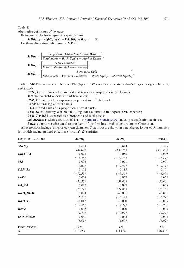
ARTICLE IN PRESS
Table 11
Alternative definitions of leverage
Estimates of the basic regression specification
MDRi;tþ1 ¼ ðkbÞX i;t þ ð1� kÞMDRi;t þ di;tþ1; (4)
for three alternative definitions of MDR:
MDR1 ¼Long Term Debtþ Short Term Debt
Total assets� Book EquityþMarket Equity
� �,
MDR2 ¼Total Liabilities
Total LiabilitiesþMarket Equity
� �,
MDR3 ¼Long term Debt
Total assets�Currrent Liabilities � Book EquityþMarket Equity
� �,
where MDR is the market debt ratio. The (lagged) ‘‘X’’ variables determine a firm’s long-run target debt ratio,
and include
EBIT_TA: earnings before interest and taxes as a proportion of total assets;
MB: the market-to-book ratio of firm assets;
DEP_TA: depreciation expense as a proportion of total assets;
LnTA: natural log of total assets;
FA-TA: fixed assets as a proportion of total assets;
R&D_DUM: dummy variable indicating that the firm did not report R&D expenses;
R&D_TA: R&D expenses as a proportion of total assets;
Ind_Median: median debt ratio of firm i’s Fama and French (2002) industry classification at time t;
Rated: dummy variable equal to one (zero) if the firm has a public debt rating in Compustat.
All regressions include (unreported) year dummies. T-statistics are shown in parentheses. Reported R2 numbers
for models including fixed effects are ‘‘within’’ R2 statistics.
Dependent variable: MDR1 MDR2 MDR3
MDRi,t 0.634 0.614 0.595
(184.09) (132.79) (153.82)
EBIT_TA �0.023 �0.055 �0.039
(�9.73) (�17.75) (�13.89)
MB 0.000 �0.001 �0.001
(0.67) (�2.47) (�2.44)
DEP_TA �0.192 �0.183 �0.191
(�12.33) (�9.33) (�9.99)
LnTA 0.020 0.028 0.024
(35.58) (39.45) (33.66)
FA_TA 0.047 0.047 0.055
(13.74) (11.03) (13.10)
R&D_DUM 0.000 �0.001 �0.001
(0.23) (�0.52) (�0.94)
R&D_TA �0.017 �0.070 �0.035
(�2.26) (�7.47) (�3.93)
Rated 0.002 0.000 0.005
(1.77) (�0.02) (2.82)
IND_Median 0.051 0.033 0.044
(6.01) (4.67) (4.92)
Fixed effects? Yes Yes Yes
N 110,253 111,088 108,476
M.J. Flannery, K.P. Rangan / Journal of Financial Economics 79 (2006) 469–506 501
ARTICLE IN PRESSM.J. Flannery, K.P. Rangan / Journal of Financial Economics 79 (2006) 469–506502
Appendix A. Estimating our dynamic panel model
Consider a (simplified) dynamic panel data model of the form:
MDRi;tþ1 ¼ aMDRi;t þ ðlþ ei;tþ1Þ, (A.1)
where i indexes firms and t indicates the time period. The error term in (A.1) has twocomponents, li, an unobserved, time-invariant, firm-specific effect, and ei,t+1, the usualresidual. Because the residual component of MDRi,t is correlated with the unobservedeffect in the error term, an OLS-estimated coefficient on MDRi,t will be biased upwards(Anderson and Hsiao, 1981; Baltagi, 2001; Bond, 2002).A common way to estimate panel data models with unobserved effects is to perform a
‘‘within’’ transform of (A.1) and then estimate using OLS. A within transformationexpresses all variables as deviations from their firm-specific time-series means. Thiseliminates mi from the regression as it is time invariant and thus provides consistentestimates. However, in the presence of a lagged dependent variable, the within transformintroduces correlation of the transformed lagged dependent variable with the transformederror term by construction (Wooldridge, 2002; Baltagi, 2001; Hsiao, 2003; etc.). To seethis, note that the within transforms of the lagged dependent variable and error terms are
MDRi;t �XTi
t¼1
MDRi;t=T i
!and ei;tþ1 �
XTi
t¼1
ei;tþ1=T i
!,
respectively, where Ti is the number of available observations for firm i. Since MDRi,2 iscorrelated with ei,2, MDRi,3 is correlated with ei,3, and so on, the transformed variables arecorrelated with the transformed error term. As a result, the coefficient on the laggeddependent variable, a, is biased downwards by a factor of (approximately) 1/T(Wooldridge, 2002). In panel data sets with large T, the bias becomes insignificant, butin panel data sets such as ours, with large N and small T, the bias can be substantial andneeds to be addressed to obtain consistent estimates.The first two columns of Table A.1 report regressions that contain biased estimates of
the lagged dependent variable’s coefficient. The OLS estimate (0.86) in column (1) is biasedupwards, while the panel estimate (0.62) in column (2) is biased downwards. As Bond(2002) points out, the true lagged dependent variable coefficient must therefore lie in theinterval (0.62, 0.86).Greene (2003) observes that we can obtain unbiased estimates of the levels regression
(A.1) via two-stage least squares if an instrument can be found that is correlated with thelagged dependent variable but not the error term. This approach forms the basis for nearlyall our results in the paper. The third column of Table A.1 reports a levels panel regressionin which the lagged book debt ratio (BDR) instruments for the lagged dependent variable.The estimated coefficient on the lagged dependent variable (0.656) lies between the OLSand ‘‘within’’ estimates, as predicted by Bond (2002).The estimates in column (3) rely on the book debt ratio being a reasonable instrument
for the market debt ratio. As always, however, finding reliable instruments can be difficultand a number of techniques have been developed in the literature to estimate unbiasedcoefficients for a model such as (A.1). (Baltagi, 2001 and Arellano and Honore, 2001provide surveys.) These alternative techniques generally first-difference the model (A.1)to eliminate fixed effects and use lagged dependent variables to instrument for the lagged

ARTICLE IN PRESS
Table A.1
Alternative methods for estimating dynamic panel regressions
In columns (1)–(3) we estimate our main regression specification that explains a firm’s market debt ratio:
MDRi;tþ1 ¼ ðkbÞX i;t þ ð1� kÞMDRi;t þ di;tþ1; (4)
In columns (4)–(6) we estimate our main regression specification in first differences:
DMDRi;tþ1 ¼ ðkbÞDX i;t � kDMDRi;t þ ðdi;tþ1 � di;tÞ
The (lagged) ‘‘X’’ variables determine a firm’s long-run target debt ratio, and include
EBIT_TA: earnings before interest and taxes as a proportion of total assets;
MB: the market-to-book ratio of firm assets;
DEP_TA: depreciation expense as a proportion of total assets;
LnTA: natural log of total assets;
FA-TA: fixed assets as a proportion of total assets;
R&D_DUM: dummy variable indicating that the firm did not report R&D expenses;
R&D_TA: R&D expenses as a proportion of total assets;
Ind_Median: median debt ratio of firm i’s Fama and French (2002) industry classification at time t; and
Rated: dummy variable equal to one if the firm has a public debt rating in Compustat, and zero otherwise.
All models include (unreported) year dummies. T-statistics are shown in parentheses. Reported R2 numbers for
models including fixed effects are ‘‘within’’ R2 statistics. For the first-differenced models, R2 cannot be computed.
(1) (2) (3) (4) (5) (6)
Simple OLS Simple FE Base
Specification,
column (7) of
Table 2
First-Difference Estimates (Anderson
and Hsiao, 1981)
Arellano and
Bond (1991)
MDRi,t�1
Instruments for
DMDRi,t
BDRi,t�1
Instruments for
DMDRi,t
MDRi,t 0.860 0.620 0.656 0.467 0.522 0.476
(457.28) (224.50) (171.58) (31.78) (20.69) (74.01)
EBIT_TA �0.025 �0.039 �0.030 �0.217 �0.221 �0.231
(�11.22) (�12.93) (�9.66) (�72.93) (�65.67) (�67.75)
MB �0.001 �0.001 0.000 �0.020 �0.020 �0.021
(�5.86) (�3.52) (�0.81) (�50.40) (�49.23) (�43.76)
DEP_TA �0.206 �0.224 �0.226 �0.269 �0.309 �0.294
(�15.62) (�10.96) (�11.06) (�10.49) (�10.27) (�10.39)
LnTA �0.001 0.027 0.025 0.125 0.128 0.131
(�3.73) (36.69) (34.00) (72.42) (63.59) (85.96)
FA_TA 0.024 0.060 0.053 0.237 0.238 0.246
(11.41) (13.52) (11.93) (37.81) (37.01) (34.38)
R&D_DUM 0.006 0.000 0.000 �0.001 �0.001 �0.002
(7.21) (�0.10) (0.02) (�0.37) (�0.23) (�0.77)
R&D_TA �0.104 �0.036 �0.025 �0.073 �0.070 �0.082
(�17.27) (�3.64) (�2.57) (�6.85) (�6.34) (�6.27)
Ind_Median 0.047 0.049 0.034 �0.137 �0.163 �0.102
(12.20) (6.32) (4.30) (�10.79) (�10.12) (-8.57)
Rated 0.005 0.005 0.003 0.025 0.024 0.021
(3.47) (2.56) (1.71) (8.71) (8.13) (6.82)
Fixed effects? No Yes Yes Noa Noa Noa
N 111,106 111,106 111,106 94,591 94,591 82,395
R2 0.753 0.467 0.466 – – –
H0: No serial
correlation
��� ���
aFixed effects are implicitly incorporated through the first-differencing procedure.���Significantly different from one at the 1% level.
M.J. Flannery, K.P. Rangan / Journal of Financial Economics 79 (2006) 469–506 503

ARTICLE IN PRESSM.J. Flannery, K.P. Rangan / Journal of Financial Economics 79 (2006) 469–506504
first-difference. For example, Anderson and Hsiao (1981) convert (A.1) into
DMDRi;tþ1 ¼ aDMDRi;t þ di;tþ1 (A.2)
and then use the dependent variable’s second lag (MDRi,t�1) to instrument for the (first-differenced) lagged dependent variable (DMDRi,t). Arellano and Bond (1991) show thatthe instrument space can include further lags of the dependent variable under somecircumstances.26
These first-difference methodologies rely on two key assumptions to produce unbiasedand consistent estimates. First, the error term ei,t+1 in (A.1) should be seriallyuncorrelated, because first-order serial correlation would make the lagged dependentvariable correlated with the (differenced) regression residual. In other words, lags of thedependent variable fail the exogeneity test if the residual is serially correlated. Second, thedependent variable should not have (near) unit root properties. If the dependent variableseries has high persistence then the first-difference will be close to zero and hence theinstruments used in the procedure will be weak.Columns (4)–(6) in Table A.1 present results based on several first-differencing methods
of estimating a dynamic panel model. These can be viewed as potential substitutes for theestimation method we use in the text for Eq. (4). Column (4) presents results based onAnderson and Hsiao (1981). We first-difference to remove the unobserved firm effects andthen use the second lag of the dependent variable as an instrument. This procedureproduces a coefficient on MDRi,t of 0.467, which is inconsistent with Bond’s (2002)assertion that the true coefficient lies between 0.62 and 0.86. We also reject the hypothesisof zero serial correlation of e in (A.1), casting serious doubt on the validity of theinstrument used. In column (5) we modify the Anderson-Hsiao method by using thesecond lag of BDR as an instrument in place of the second lag of MDR. This instrumentshould be immune to the serial correlation problem identified in column (4). We find thatthe estimate (0.522) is higher than column (4)’s, but still outside the interval defined by theOLS and ‘‘within’’ estimates. The problem appears to be that of weak instruments givenpersistence in the dependent variable. Indeed, the correlation in the lagged levels of ourdependent variable is 0.98.Given the serial correlation in the error terms and the high persistence in our dependent
variable, Arellano and Bond’s (1991) GMM procedure is unlikely to yield consistentresults. To verify, we run the GMM estimation (using Stata’s XTABOND procedure) andpresent the results in column (6). The coefficient on MDRi,t (0.476) implies very rapidadjustment, but both the tests of serial correlation and an (unreported) Sargan test ofoveridentifying restrictions are rejected at the 1% level. Arellano and Bond’s (1991)technique thus cannot be applied to our data.
References
Ahn, S., Schmidt, P., 1995. Efficient estimation of models for dynamic panel data. Journal of Econometrics 68,
5–28.
Alti, Aydogan, 2004. How persistent is the impact of market timing on capital structure? University of Texas
Working paper.
26Subsequent authors refine Arellano and Bond’s (1991) General Methods of Moments procedures (e.g.,
Arellano and Bover, 1995; Ahn and Schmidt, 1995).

ARTICLE IN PRESSM.J. Flannery, K.P. Rangan / Journal of Financial Economics 79 (2006) 469–506 505
Anderson, T., Hsiao, C., 1981. Estimation of dynamic models with error components. Journal of the American
Statistical Association 76, 598–606.
Arellano, M., Bond, S., 1991. Some tests of specification for panel data: Monte-Carlo evidence and an application
to employment equations. Review of Economic Studies 38, 277–297.
Arellano, M., Bover, O., 1995. Another look at instrumental-variable estimation of error-components models.
Journal of Econometrics 68, 29–52.
Arellano, M., Honore, B., 2001. Panel data models: some recent developments, In: Heckman, J.J., Learner, E.E.,
(Eds.), Handbook of Econometrics, vol 5, North-Holland, Amsterdam.
Baker, M., Wurgler, J., 2002. Market timing and capital structure. The Journal of Finance 57, 1–32.
Baltagi, B., 2001. Econometric Analysis of Panel Data, 2nd edn. John Wiley, New York.
Bond, S., 2002. Dynamic panel data models: a guide to micro data methods and practice. Working paper.
Donaldson, G., 1961. Corporate debt capacity: a study of corporate debt policy and the determination of
corporate debt capacity. Harvard Business School, Division of Research, Harvard University.
Fama, E., French, K., 1997. Industry costs of equity. Journal of Financial Economics 43, 153–193.
Fama, E., French, K., 2002. Testing trade-off and pecking order predictions about dividends and debt. Review of
Financial Studies 15, 1–34.
Fama, E., MacBeth, J., 1973. Risk, return, and equilibrium: empirical tests. Journal of Political Economy 81,
607–636.
Faulkender, M., Petersen, M., 2005. Does the source of capital affect capital structure? Review of Financial
Studies, forthcoming.
Fischer, E., Heinkel, R., Zechner, J., 1989. Dynamic capital structure choice: theory and tests. Journal of Finance
44, 19–40.
Frank, M., Goyal, V., 2003. Testing the pecking order theory of capital structure. Journal of Financial Economics
67, 217–248.
Graham, J., Harvey, C., 2001. The theory and practice of corporate finance: evidence from the field. Journal of
Financial Economics 60, 187–243.
Greene, W., 2003. Econometric Analysis, 5th edn. Upper Saddle River, Prentice Hall.
Halov, N., Heider, F., 2004. Capital structure, risk and asymmetric information. NYU Working paper.
Hovakimian, A., 2003. Are observed capital structures determined by equity market timing? Baruch College
Working paper.
Hovakimian, A., Opler, T., Titman, S., 2001. The debt-equity choice: an analysis of issuing firms. Journal of
Financial and Quantitative Analysis 36, 1–24.
Hovakimian, A., Hovakimian, G., Tehranian, H., 2004. Determinants of target capital structure: the case of dual
debt and equity issues. Journal of Financial Economics 71, 517–540.
Hsiao, C., 2003. Analysis of Panel Data, 2nd edn. Cambridge University Press, Cambridge.
Huang, R., Ritter, J., 2005. Testing the market timing theory of capital structure. University of Florida Working
paper.
Jalilvand, A., Harris, R., 1984. Corporate behaviour in adjusting to capital structure and dividend targets: an
econometric study. Journal of Finance 39, 127–145.
Ju, N., Parino, R., Poteshman, A., Weisbach, M., 2002. Horses and rabbits optimal dynamic capital structure
from shareholder and manager perspectives. Working paper.
Kayhan, A., Titman, S., 2005. Firms’ histories and their capital structure. University of Texas Working paper.
Korajczyk, R., Levy, A., 2003. Capital structure choice: macroeconomic conditions and financial constraints.
Journal of Financial Economics 68, 75–109.
Leary, M., Roberts, M., 2005. Do firms rebalance their capital structure? Journal of Finance forthcoming.
Lemmon, M., Zender, J., 2004. Debt capacity and tests of capital structure theories. University of Utah and
University of Colorado Working paper.
Marcus, A., 1983. The bank capital decision: a time series-cross section analysis. Journal of Finance 38, 1217–1232.
Marsh, P., 1982. The choice between equity and debt: an empirical study. Journal of Finance 37, 121–144.
Mauer, D., Triantis, A., 1994. Interactions of corporate financing and investment decisions: a dynamic
framework. Journal of Finance 49, 1253–1277.
Modigliani, F., Miller, M., 1958. The cost of capital, corporation finance, and the theory of investment. American
Economic Review 48, 655–669.
Myers, S., 1984. The capital structure puzzle. The Journal of Finance 39, 575–592.
Rajan, R., Zingales, L., 1995. What do we know about capital structure: some evidence from international data.
Journal of Finance 50, 1421–1460.

ARTICLE IN PRESSM.J. Flannery, K.P. Rangan / Journal of Financial Economics 79 (2006) 469–506506
Roberts, M., 2002. The dynamics of capital structure: an empirical analysis of a partially observable system. Duke
Working paper.
Shyam-Sunder, L., Myers, S., 1999. Testing static tradeoff against pecking order models of capital structure.
Journal of Financial Economics 51, 219–243.
Titman, S. Tsyplakov, S., 2004. A dynamic model of optimal capital structure. University of Texas Working
paper.
Welch, I., 2004. Capital structure and stock returns. Journal of Political Economy 112, 106–131.
Wooldridge, J., 2002. Econometric Analysis of Cross Section and Panel Data. The MIT Press, Cambridge.