Embed Size (px)
DESCRIPTION
Tensor Calculus
Citation preview
108
§1.4 DERIVATIVE OF A TENSOR
In this section we develop some additional operations associated with tensors. Historically, one of the
basic problems of the tensor calculus was to try and find a tensor quantity which is a function of the metric
tensor gij and some of its derivatives∂gij
∂xm,
∂2gij
∂xm∂xn, . . . . A solution of this problem is the fourth order
Riemann Christoffel tensor Rijkl to be developed shortly. In order to understand how this tensor was arrived
at, we must first develop some preliminary relationships involving Christoffel symbols.
Christoffel Symbols
Let us consider the metric tensor gij which we know satisfies the transformation law
gαβ = gab∂xa
∂xα
∂xb
∂xβ.
Define the quantity
(α, β, γ) =∂gαβ
∂xγ =∂gab
∂xc
∂xc
∂xγ
∂xa
∂xα
∂xb
∂xβ+ gab
∂2xa
∂xα∂xγ
∂xb
∂xβ+ gab
∂xa
∂xα
∂2xb
∂xβ∂xγ
and form the combination of terms12
[(α, β, γ) + (β, γ, α)− (γ, α, β)] to obtain the result
12
[∂gαβ
∂xγ +∂gβγ
∂xα − ∂gγα
∂xβ
]=
12
[∂gab
∂xc+
∂gbc
∂xa− ∂gca
∂xb
]∂xa
∂xα
∂xb
∂xβ
∂xc
∂xγ + gab∂xb
∂xβ
∂2xa
∂xα∂xγ . (1.4.1)
In this equation the combination of derivatives occurring inside the brackets is called a Christoffel symbol
of the first kind and is defined by the notation
[ac, b] = [ca, b] =12
[∂gab
∂xc+
∂gbc
∂xa− ∂gac
∂xb
]. (1.4.2)
The equation (1.4.1) defines the transformation for a Christoffel symbol of the first kind and can be expressed
as
[α γ, β] = [ac, b]∂xa
∂xα
∂xb
∂xβ
∂xc
∂xγ + gab∂2xa
∂xα∂xγ
∂xb
∂xβ. (1.4.3)
Observe that the Christoffel symbol of the first kind [ac, b] does not transform like a tensor. However, it is
symmetric in the indices a and c.
At this time it is convenient to use the equation (1.4.3) to develop an expression for the second derivative
term which occurs in that equation as this second derivative term arises in some of our future considerations.
To solve for this second derivative we can multiply equation (1.4.3) by∂xβ
∂xdgde and simplify the result to the
form∂2xe
∂xα∂xγ = −gde[ac, d]∂xa
∂xα
∂xc
∂xγ + [α γ, β]∂xβ
∂xdgde. (1.4.4)
The transformation gde = gλµ ∂xd
∂xλ
∂xe
∂xµ allows us to express the equation (1.4.4) in the form
∂2xe
∂xα∂xγ = −gde[ac, d]∂xa
∂xα
∂xc
∂xγ + gβµ[α γ, β]∂xe
∂xµ . (1.4.5)
109
Define the Christoffel symbol of the second kind as
{i
j k
}={
i
k j
}= giα[jk, α] =
12giα
(∂gkα
∂xj+
∂gjα
∂xk− ∂gjk
∂xα
). (1.4.6)
This Christoffel symbol of the second kind is symmetric in the indices j and k and from equation (1.4.5) we
see that it satisfies the transformation law
{µ
α γ
}∂xe
∂xµ ={
e
a c
}∂xa
∂xα
∂xc
∂xγ +∂2xe
∂xα∂xγ . (1.4.7)
Observe that the Christoffel symbol of the second kind does not transform like a tensor quantity. We can use
the relation defined by equation (1.4.7) to express the second derivative of the transformation equations in
terms of the Christoffel symbols of the second kind. At times it will be convenient to represent the Christoffel
symbols with a subscript to indicate the metric from which they are calculated. Thus, an alternative notation
for{
i
j k
}is the notation
{i
j k
}g
.
EXAMPLE 1.4-1. (Christoffel symbols) Solve for the Christoffel symbol of the first kind in terms of
the Christoffel symbol of the second kind.
Solution: By the definition from equation (1.4.6) we have
{i
j k
}= giα[jk, α].
We multiply this equation by gβi and find
gβi
{i
j k
}= δα
β [jk, α] = [jk, β]
and so
[jk, α] = gαi
{i
j k
}= gα1
{1
j k
}+ · · · + gαN
{N
j k
}.
EXAMPLE 1.4-2. (Christoffel symbols of first kind)
Derive formulas to find the Christoffel symbols of the first kind in a generalized orthogonal coordinate
system with metric coefficients
gij = 0 for i 6= j and g(i)(i) = h2(i), i = 1, 2, 3
where i is not summed.
Solution: In an orthogonal coordinate system where gij = 0 for i 6= j we observe that
[ab, c] =12
(∂gac
∂xb+
∂gbc
∂xa− ∂gab
∂xc
). (1.4.8)
Here there are 33 = 27 quantities to calculate. We consider the following cases:
110
CASE I Let a = b = c = i, then the equation (1.4.8) simplifies to
[ab, c] = [ii, i] =12
∂gii
∂xi(no summation on i). (1.4.9)
From this equation we can calculate any of the Christoffel symbols
[11, 1], [22, 2], or [33, 3].
CASE II Let a = b = i 6= c, then the equation (1.4.8) simplifies to the form
[ab, c] = [ii, c] = −12
∂gii
∂xc(no summation on i and i 6= c). (1.4.10)
since, gic = 0 for i 6= c. This equation shows how we may calculate any of the six Christoffel symbols
[11, 2], [11, 3], [22, 1], [22, 3], [33, 1], [33, 2].
CASE III Let a = c = i 6= b, and noting that gib = 0 for i 6= b, it can be verified that the equation (1.4.8)
simplifies to the form
[ab, c] = [ib, i] = [bi, i] =12
∂gii
∂xb(no summation on i and i 6= b). (1.4.11)
From this equation we can calculate any of the twelve Christoffel symbols
[12, 1] = [21, 1]
[32, 3] = [23, 3]
[13, 1] = [31, 1]
[31, 3] = [13, 3]
[21, 2] = [12, 2]
[23, 2] = [32, 2]
CASE IV Let a 6= b 6= c and show that the equation (1.4.8) reduces to
[ab, c] = 0, (a 6= b 6= c.)
This represents the six Christoffel symbols
[12, 3] = [21, 3] = [23, 1] = [32, 1] = [31, 2] = [13, 2] = 0.
From the Cases I,II,III,IV all twenty seven Christoffel symbols of the first kind can be determined. In
practice, only the nonzero Christoffel symbols are listed.
EXAMPLE 1.4-3. (Christoffel symbols of the first kind)Find the nonzero Christoffel symbols of the
first kind in cylindrical coordinates.
Solution: From the results of example 1.4-2 we find that for x1 = r, x2 = θ, x3 = z and
g11 = 1, g22 = (x1)2 = r2, g33 = 1
the nonzero Christoffel symbols of the first kind in cylindrical coordinates are:
[22, 1] = −12
∂g22
∂x1= −x1 = −r
[21, 2] = [12, 2] =12
∂g22
∂x1= x1 = r.
111
EXAMPLE 1.4-4. (Christoffel symbols of the second kind)
Find formulas for the calculation of the Christoffel symbols of the second kind in a generalized orthogonal
coordinate system with metric coefficients
gij = 0 for i 6= j and g(i)(i) = h2(i), i = 1, 2, 3
where i is not summed.
Solution: By definition we have
{i
j k
}= gim[jk, m] = gi1[jk, 1] + gi2[jk, 2] + gi3[jk, 3] (1.4.12)
By hypothesis the coordinate system is orthogonal and so
gij = 0 for i 6= j and gii =1gii
i not summed.
The only nonzero term in the equation (1.4.12) occurs when m = i and consequently
{i
j k
}= gii[jk, i] =
[jk, i]gii
no summation on i. (1.4.13)
We can now consider the four cases considered in the example 1.4-2.
CASE I Let j = k = i and show
{i
i i
}=
[ii, i]gii
=1
2gii
∂gii
∂xi=
12
∂
∂xiln gii no summation on i. (1.4.14)
CASE II Let k = j 6= i and show
{i
j j
}=
[jj, i]gii
=−12gii
∂gjj
∂xino summation on i or j. (1.4.15)
CASE III Let i = j 6= k and verify that
{j
j k
}={
j
k j
}=
[jk, j]gjj
=1
2gjj
∂gjj
∂xk=
12
∂
∂xkln gjj no summation on i or j. (1.4.16)
CASE IV For the case i 6= j 6= k we find
{i
j k
}=
[jk, i]gii
= 0, i 6= j 6= k no summation on i.
The above cases represent all 27 terms.
112
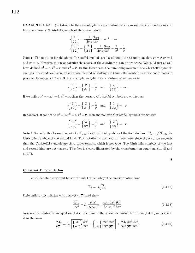
EXAMPLE 1.4-5. (Notation) In the case of cylindrical coordinates we can use the above relations and
find the nonzero Christoffel symbols of the second kind:{12 2
}= − 1
2g11
∂g22
∂x1= −x1 = −r{
21 2
}={
22 1
}=
12g22
∂g22
∂x1=
1x1
=1r
Note 1: The notation for the above Christoffel symbols are based upon the assumption that x1 = r, x2 = θ
and x3 = z. However, in tensor calculus the choice of the coordinates can be arbitrary. We could just as well
have defined x1 = z, x2 = r and x3 = θ. In this latter case, the numbering system of the Christoffel symbols
changes. To avoid confusion, an alternate method of writing the Christoffel symbols is to use coordinates in
place of the integers 1,2 and 3. For example, in cylindrical coordinates we can write{θ
r θ
}={
θ
θ r
}=
1r
and{
r
θ θ
}= −r.
If we define x1 = r, x2 = θ, x3 = z, then the nonzero Christoffel symbols are written as{2
1 2
}={
22 1
}=
1r
and{
12 2
}= −r.
In contrast, if we define x1 = z, x2 = r, x3 = θ, then the nonzero Christoffel symbols are written{3
2 3
}={
33 2
}=
1r
and{
23 3
}= −r.
Note 2: Some textbooks use the notation Γa,bc for Christoffel symbols of the first kind and Γdbc = gdaΓa,bc for
Christoffel symbols of the second kind. This notation is not used in these notes since the notation suggests
that the Christoffel symbols are third order tensors, which is not true. The Christoffel symbols of the first
and second kind are not tensors. This fact is clearly illustrated by the transformation equations (1.4.3) and
(1.4.7).
Covariant Differentiation
Let Ai denote a covariant tensor of rank 1 which obeys the transformation law
Aα = Ai∂xi
∂xα . (1.4.17)
Differentiate this relation with respect to xβ and show
∂Aα
∂xβ= Ai
∂2xi
∂xα∂xβ+
∂Ai
∂xj
∂xj
∂xβ
∂xi
∂xα . (1.4.18)
Now use the relation from equation (1.4.7) to eliminate the second derivative term from (1.4.18) and express
it in the form∂Aα
∂xβ= Ai
[{σ
α β
}∂xi
∂xσ −{
i
j k
}∂xj
∂xα
∂xk
∂xβ
]+
∂Ai
∂xj
∂xj
∂xβ
∂xi
∂xα . (1.4.19)
113
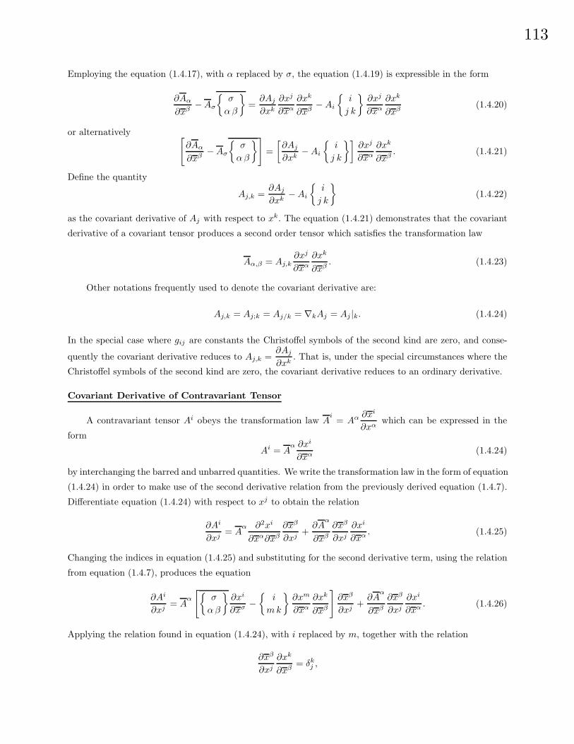
Employing the equation (1.4.17), with α replaced by σ, the equation (1.4.19) is expressible in the form
∂Aα
∂xβ−Aσ
{σ
α β
}=
∂Aj
∂xk
∂xj
∂xα
∂xk
∂xβ−Ai
{i
j k
}∂xj
∂xα
∂xk
∂xβ(1.4.20)
or alternatively [∂Aα
∂xβ−Aσ
{σ
α β
}]=[∂Aj
∂xk−Ai
{i
j k
}]∂xj
∂xα
∂xk
∂xβ. (1.4.21)
Define the quantity
Aj,k =∂Aj
∂xk−Ai
{i
j k
}(1.4.22)
as the covariant derivative of Aj with respect to xk. The equation (1.4.21) demonstrates that the covariant
derivative of a covariant tensor produces a second order tensor which satisfies the transformation law
Aα,β = Aj,k∂xj
∂xα
∂xk
∂xβ. (1.4.23)
Other notations frequently used to denote the covariant derivative are:
Aj,k = Aj;k = Aj/k = ∇kAj = Aj |k. (1.4.24)
In the special case where gij are constants the Christoffel symbols of the second kind are zero, and conse-
quently the covariant derivative reduces to Aj,k =∂Aj
∂xk. That is, under the special circumstances where the
Christoffel symbols of the second kind are zero, the covariant derivative reduces to an ordinary derivative.
Covariant Derivative of Contravariant Tensor
A contravariant tensor Ai obeys the transformation law Ai
= Aα ∂xi
∂xαwhich can be expressed in the
form
Ai = Aα ∂xi
∂xα (1.4.24)
by interchanging the barred and unbarred quantities. We write the transformation law in the form of equation
(1.4.24) in order to make use of the second derivative relation from the previously derived equation (1.4.7).
Differentiate equation (1.4.24) with respect to xj to obtain the relation
∂Ai
∂xj= A
α ∂2xi
∂xα∂xβ
∂xβ
∂xj+
∂Aα
∂xβ
∂xβ
∂xj
∂xi
∂xα . (1.4.25)
Changing the indices in equation (1.4.25) and substituting for the second derivative term, using the relation
from equation (1.4.7), produces the equation
∂Ai
∂xj= A
α
[{σ
α β
}∂xi
∂xσ −{
i
m k
}∂xm
∂xα
∂xk
∂xβ
]∂xβ
∂xj+
∂Aα
∂xβ
∂xβ
∂xj
∂xi
∂xα . (1.4.26)
Applying the relation found in equation (1.4.24), with i replaced by m, together with the relation
∂xβ
∂xj
∂xk
∂xβ= δk
j ,
114
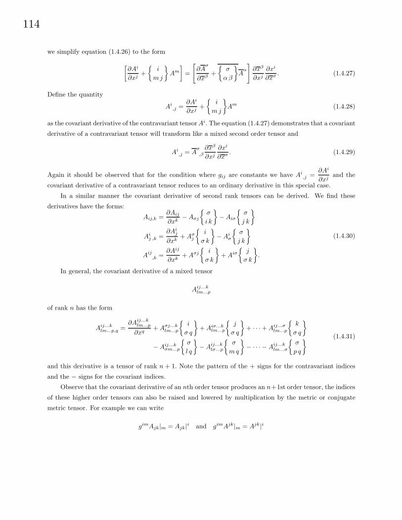
we simplify equation (1.4.26) to the form
[∂Ai
∂xj+{
i
m j
}Am
]=
[∂A
σ
∂xβ+{
σ
α β
}A
α
]∂xβ
∂xj
∂xi
∂xσ . (1.4.27)
Define the quantity
Ai,j =
∂Ai
∂xj+{
i
m j
}Am (1.4.28)
as the covariant derivative of the contravariant tensor Ai. The equation (1.4.27) demonstrates that a covariant
derivative of a contravariant tensor will transform like a mixed second order tensor and
Ai,j = A
σ
,β
∂xβ
∂xj
∂xi
∂xσ . (1.4.29)
Again it should be observed that for the condition where gij are constants we have Ai,j =
∂Ai
∂xjand the
covariant derivative of a contravariant tensor reduces to an ordinary derivative in this special case.
In a similar manner the covariant derivative of second rank tensors can be derived. We find these
derivatives have the forms:
Aij,k =∂Aij
∂xk−Aσj
{σ
i k
}−Aiσ
{σ
j k
}
Aij ,k =
∂Aij
∂xk+ Aσ
j
{i
σ k
}−Ai
σ
{σ
j k
}
Aij,k =
∂Aij
∂xk+ Aσj
{i
σ k
}+ Aiσ
{j
σ k
}.
(1.4.30)
In general, the covariant derivative of a mixed tensor
Aij...klm...p
of rank n has the form
Aij...klm...p,q =
∂Aij...klm...p
∂xq+ Aσj...k
lm...p
{i
σ q
}+ Aiσ...k
lm...p
{j
σ q
}+ · · · + Aij...σ
lm...p
{k
σ q
}
−Aij...kσm...p
{σ
l q
}−Aij...k
lσ...p
{σ
m q
}− · · · −Aij...k
lm...σ
{σ
p q
} (1.4.31)
and this derivative is a tensor of rank n + 1. Note the pattern of the + signs for the contravariant indices
and the − signs for the covariant indices.
Observe that the covariant derivative of an nth order tensor produces an n+1st order tensor, the indices
of these higher order tensors can also be raised and lowered by multiplication by the metric or conjugate
metric tensor. For example we can write
gimAjk|m = Ajk|i and gimAjk|m = Ajk|i
115
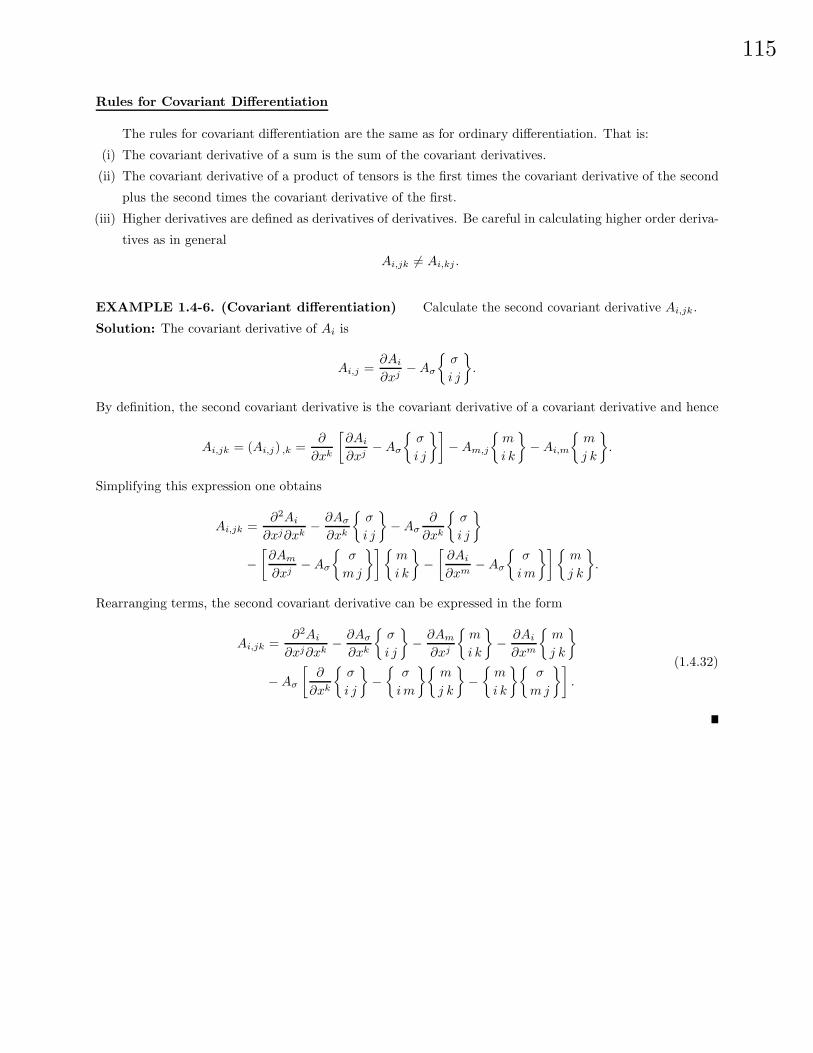
Rules for Covariant Differentiation
The rules for covariant differentiation are the same as for ordinary differentiation. That is:
(i) The covariant derivative of a sum is the sum of the covariant derivatives.
(ii) The covariant derivative of a product of tensors is the first times the covariant derivative of the second
plus the second times the covariant derivative of the first.
(iii) Higher derivatives are defined as derivatives of derivatives. Be careful in calculating higher order deriva-
tives as in general
Ai,jk 6= Ai,kj .
EXAMPLE 1.4-6. (Covariant differentiation) Calculate the second covariant derivative Ai,jk.
Solution: The covariant derivative of Ai is
Ai,j =∂Ai
∂xj−Aσ
{σ
i j
}.
By definition, the second covariant derivative is the covariant derivative of a covariant derivative and hence
Ai,jk = (Ai,j) ,k =∂
∂xk
[∂Ai
∂xj−Aσ
{σ
i j
}]−Am,j
{m
i k
}−Ai,m
{m
j k
}.
Simplifying this expression one obtains
Ai,jk =∂2Ai
∂xj∂xk− ∂Aσ
∂xk
{σ
i j
}−Aσ
∂
∂xk
{σ
i j
}
−[∂Am
∂xj−Aσ
{σ
m j
}]{m
i k
}−[
∂Ai
∂xm−Aσ
{σ
i m
}]{m
j k
}.
Rearranging terms, the second covariant derivative can be expressed in the form
Ai,jk =∂2Ai
∂xj∂xk− ∂Aσ
∂xk
{σ
i j
}− ∂Am
∂xj
{m
i k
}− ∂Ai
∂xm
{m
j k
}
−Aσ
[∂
∂xk
{σ
i j
}−{
σ
i m
}{m
j k
}−{
m
i k
}{σ
m j
}].
(1.4.32)
116
Riemann Christoffel Tensor
Utilizing the equation (1.4.32), it is left as an exercise to show that
Ai,jk −Ai,kj = AσRσijk
where
Rσijk =
∂
∂xj
{σ
i k
}− ∂
∂xk
{σ
i j
}+{
m
i k
}{σ
m j
}−{
m
i j
}{σ
m k
}(1.4.33)
is called the Riemann Christoffel tensor. The covariant form of this tensor is
Rhjkl = gihRijkl. (1.4.34)
It is an easy exercise to show that this covariant form can be expressed in either of the forms
Rinjk =∂
∂xj[nk, i]− ∂
∂xk[nj, i] + [ik, s]
{s
n j
}− [ij, s]
{s
n k
}
or Rijkl =12
(∂2gil
∂xj∂xk− ∂2gjl
∂xi∂xk− ∂2gik
∂xj∂xl+
∂2gjk
∂xi∂xl
)+ gαβ ([jk, β][il, α]− [jl, β][ik, α]) .
From these forms we find that the Riemann Christoffel tensor is skew symmetric in the first two indices
and the last two indices as well as being symmetric in the interchange of the first pair and last pairs of
indices and consequently
Rjikl = −Rijkl Rijlk = −Rijkl Rklij = Rijkl .
In a two dimensional space there are only four components of the Riemann Christoffel tensor to consider.
These four components are either +R1212 or −R1212 since they are all related by
R1212 = −R2112 = R2121 = −R1221.
In a Cartesian coordinate system Rhijk = 0. The Riemann Christoffel tensor is important because it occurs
in differential geometry and relativity which are two areas of interest to be considered later. Additional
properties of this tensor are found in the exercises of section 1.5.
117
Physical Interpretation of Covariant Differentiation
In a system of generalized coordinates (x1, x2, x3) we can construct the basis vectors ( ~E1, ~E2, ~E3). These
basis vectors change with position. That is, each basis vector is a function of the coordinates at which they
are evaluated. We can emphasize this dependence by writing
~Ei = ~Ei(x1, x2, x3) =∂~r
∂xii = 1, 2, 3.
Associated with these basis vectors we have the reciprocal basis vectors
~Ei = ~Ei(x1, x2, x3), i = 1, 2, 3
which are also functions of position. A vector ~A can be represented in terms of contravariant components as
~A = A1 ~E1 + A2 ~E2 + A3 ~E3 = Aj ~Ej (1.4.35)
or it can be represented in terms of covariant components as
~A = A1~E1 + A2
~E2 + A3~E3 = Aj
~Ej . (1.4.36)
A change in the vector ~A is represented as
d ~A =∂ ~A
∂xkdxk
where from equation (1.4.35) we find
∂ ~A
∂xk= Aj ∂ ~Ej
∂xk+
∂Aj
∂xk~Ej (1.4.37)
or alternatively from equation (1.4.36) we may write
∂ ~A
∂xk= Aj
∂ ~Ej
∂xk+
∂Aj
∂xk~Ej . (1.4.38)
We define the covariant derivative of the covariant components as
Ai,k =∂ ~A
∂xk· ~Ei =
∂Ai
∂xk+ Aj
∂ ~Ej
∂xk· ~Ei. (1.4.39)
The covariant derivative of the contravariant components are defined by the relation
Ai,k =
∂ ~A
∂xk· ~Ei =
∂Ai
∂xk+ Aj ∂ ~Ej
∂xk· ~Ei. (1.4.40)
Introduce the notation
∂ ~Ej
∂xk={
m
j k
}~Em and
∂ ~Ej
∂xk= −
{j
m k
}~Em. (1.4.41)
We then have~Ei · ∂ ~Ej
∂xk={
m
j k
}~Em · ~Ei =
{m
j k
}δim =
{i
j k
}(1.4.42)
118
and~Ei · ∂ ~Ej
∂xk= −
{j
m k
}~Em · ~Ei = −
{j
m k
}δmi = −
{j
i k
}. (1.4.43)
Then equations (1.4.39) and (1.4.40) become
Ai,k =∂Ai
∂xk−{
j
i k
}Aj
Ai,k =
∂Ai
∂xk+{
i
j k
}Aj ,
which is consistent with our earlier definitions from equations (1.4.22) and (1.4.28). Here the first term of
the covariant derivative represents the rate of change of the tensor field as we move along a coordinate curve.
The second term in the covariant derivative represents the change in the local basis vectors as we move
along the coordinate curves. This is the physical interpretation associated with the Christoffel symbols of
the second kind.
We make the observation that the derivatives of the basis vectors in equations (1.4.39) and (1.4.40) are
related since~Ei · ~Ej = δj
i
and consequently∂
∂xk( ~Ei · ~Ej) = ~Ei · ∂ ~Ej
∂xk+
∂ ~Ei
∂xk· ~Ej = 0
or ~Ei · ∂ ~Ej
∂xk= − ~Ej · ∂ ~Ei
∂xk
Hence we can express equation (1.4.39) in the form
Ai,k =∂Ai
∂xk−Aj
~Ej · ∂ ~Ei
∂xk. (1.4.44)
We write the first equation in (1.4.41) in the form
∂ ~Ej
∂xk={
m
j k
}gim
~Ei = [jk, i] ~Ei (1.4.45)
and consequently∂ ~Ej
∂xk· ~Em =
{i
j k
}~Ei · ~Em =
{i
j k
}δmi =
{m
j k
}
and∂ ~Ej
∂xk· ~Em =[jk, i] ~Ei · ~Em = [jk, i]δi
m = [jk, m].
(1.4.46)
These results also reduce the equations (1.4.40) and (1.4.44) to our previous forms for the covariant deriva-
tives.
The equations (1.4.41) are representations of the vectors ∂ ~Ei
∂xk and ∂ ~Ej
∂xk in terms of the basis vectors and
reciprocal basis vectors of the space. The covariant derivative relations then take into account how these
vectors change with position and affect changes in the tensor field.
The Christoffel symbols in equations (1.4.46) are symmetric in the indices j and k since
∂ ~Ej
∂xk=
∂
∂xk
(∂~r
∂xj
)=
∂
∂xj
(∂~r
∂xk
)=
∂ ~Ek
∂xj. (1.4.47)
119
The equations (1.4.46) and (1.4.47) enable us to write
[jk, m] =~Em · ∂ ~Ej
∂xk=
12
[~Em · ∂ ~Ej
∂xk+ ~Em · ∂ ~Ek
∂xj
]
=12
[∂
∂xk
(~Em · ~Ej
)+
∂
∂xj
(~Em · ~Ek
)− ~Ej · ∂ ~Em
∂xk− ~Ek · ∂ ~Em
∂xj
]
=12
[∂
∂xk
(~Em · ~Ej
)+
∂
∂xj
(~Em · ~Ek
)− ~Ej · ∂ ~Ek
∂xm− ~Ek · ∂ ~Ej
∂xm
]
=12
[∂
∂xk
(~Em · ~Ej
)+
∂
∂xj
(~Em · ~Ek
)− ∂
∂xm
(~Ej · ~Ek
)]
=12
[∂gmj
∂xk+
∂gmk
∂xj− ∂gjk
∂xm
]= [kj, m]
which again agrees with our previous result.
For future reference we make the observation that if the vector ~A is represented in the form ~A = Aj ~Ej ,
involving contravariant components, then we may write
d ~A =∂ ~A
∂xkdxk =
(∂Aj
∂xk~Ej + Aj ∂ ~Ej
∂xk
)dxk
=(
∂Aj
∂xk~Ej + Aj
{i
j k
}~Ei
)dxk
=(
∂Aj
∂xk+{
j
m k
}Am
)~Ej dxk = Aj
,k dxk ~Ej .
(1.4.48)
Similarly, if the vector ~A is represented in the form ~A = Aj~Ej involving covariant components it is left as
an exercise to show that
d ~A = Aj,k dxk ~Ej (1.4.49)
Ricci’s Theorem
Ricci’s theorem states that the covariant derivative of the metric tensor vanishes and gik,l = 0.
Proof: We have
gik,l =∂gik
∂xl−{
m
k l
}gim −
{m
i l
}gmk
gik,l =∂gik
∂xl− [kl, i]− [il, k]
gik,l =∂gik
∂xl− 1
2
[∂gik
∂xl+
∂gil
∂xk− ∂gkl
∂xi
]− 1
2
[∂gik
∂xl+
∂gkl
∂xi− ∂gil
∂xk
]= 0.
Because of Ricci’s theorem the components of the metric tensor can be regarded as constants during covariant
differentiation.
EXAMPLE 1.4-7. (Covariant differentiation) Show that δij,k = 0.
Solution
δij,k =
∂δij
∂xk+ δσ
j
{i
σ k
}− δi
σ
{σ
j k
}={
i
j k
}−{
i
j k
}= 0.
120
EXAMPLE 1.4-8. (Covariant differentiation) Show that gij,k = 0.
Solution: Since gijgjk = δk
i we take the covariant derivative of this expression and find
(gijgjk),l = δk
i,l = 0
gijgjk
,l + gij,lgjk = 0.
But gij,l = 0 by Ricci’s theorem and hence gijgjk
,l = 0. We multiply this expression by gim and obtain
gimgijgjk
,l = δmj gjk
,l = gmk,l = 0
which demonstrates that the covariant derivative of the conjugate metric tensor is also zero.
EXAMPLE 1.4-9. (Covariant differentiation) Some additional examples of covariant differentiation
are:(i) (gilA
l),k = gilAl,k = Ai,k
(ii) (gimgjnAij) ,k = gimgjnAij,k = Amn,k
Intrinsic or Absolute Differentiation
The intrinsic or absolute derivative of a covariant vector Ai taken along a curve xi = xi(t), i = 1, . . . , N
is defined as the inner product of the covariant derivative with the tangent vector to the curve. The intrinsic
derivative is representedδAi
δt= Ai,j
dxj
dt
δAi
δt=[∂Ai
∂xj−Aα
{α
i j
}]dxj
dt
δAi
δt=
dAi
dt−Aα
{α
i j
}dxj
dt.
(1.4.50)
Similarly, the absolute or intrinsic derivative of a contravariant tensor Ai is represented
δAi
δt= Ai
,j
dxj
dt=
dAi
dt+{
i
j k
}Ak dxj
dt.
The intrinsic or absolute derivative is used to differentiate sums and products in the same manner as used
in ordinary differentiation. Also if the coordinate system is Cartesian the intrinsic derivative becomes an
ordinary derivative.
The intrinsic derivative of higher order tensors is similarly defined as an inner product of the covariant
derivative with the tangent vector to the given curve. For example,
δAijklm
δt= Aij
klm,p
dxp
dt
is the intrinsic derivative of the fifth order mixed tensor Aijklm.
121
EXAMPLE 1.4-10. (Generalized velocity and acceleration) Let t denote time and let xi = xi(t)
for i = 1, . . . , N , denote the position vector of a particle in the generalized coordinates (x1, . . . , xN ). From
the transformation equations (1.2.30), the position vector of the same particle in the barred system of
coordinates, (x1, x2, . . . , xN ), is
xi = xi(x1(t), x2(t), . . . , xN (t)) = xi(t), i = 1, . . . , N.
The generalized velocity is vi = dxi
dt , i = 1, . . . , N. The quantity vi transforms as a tensor since by definition
vi =dxi
dt=
∂xi
∂xj
dxj
dt=
∂xi
∂xjvj . (1.4.51)
Let us now find an expression for the generalized acceleration. Write equation (1.4.51) in the form
vj = vi ∂xj
∂xi (1.4.52)
and differentiate with respect to time to obtain
dvj
dt= vi ∂2xj
∂xi∂xk
dxk
dt+
dvi
dt
∂xj
∂xi (1.4.53)
The equation (1.4.53) demonstrates that dvi
dt does not transform like a tensor. From the equation (1.4.7)
previously derived, we change indices and write equation (1.4.53) in the form
dvj
dt= vi dxk
dt
[{σ
i k
}∂xj
∂xσ −{
j
a c
}∂xa
∂xi
∂xc
∂xk
]+
∂xj
∂xi
dvi
dt.
Rearranging terms we find
∂vj
∂xk
dxk
dt+{
j
a c
}(∂xa
∂xivi
)(∂xc
∂xk
dxk
dt
)=
∂xj
∂xi
∂vi
∂xk
dxk
dt+{
σ
i k
}vi ∂xj
∂xσ
dxk
dtor
[∂vj
∂xk+{
j
a k
}va
]dxk
dt=
[∂vσ
∂xk+{
σ
i k
}vi
]dxk
dt
∂xj
∂xσ
δvj
δt=
δvσ
δt
∂xj
∂xσ .
The above equation illustrates that the intrinsic derivative of the velocity is a tensor quantity. This derivative
is called the generalized acceleration and is denoted
f i =δvi
δt= vi
,j
dxj
dt=
dvi
dt+{
i
m n
}vmvn =
d2xi
dt2+{
i
m n
}dxm
dt
dxn
dt, i = 1, . . . , N (1.4.54)
To summarize, we have shown that if
xi = xi(t), i = 1, . . . , N is the generalized position vector, then
vi =dxi
dt, i = 1, . . . , N is the generalized velocity, and
f i =δvi
δt= vi
,j
dxj
dt, i = 1, . . . , N is the generalized acceleration.
122
Parallel Vector Fields
Let yi = yi(t), i = 1, 2, 3 denote a space curve C in a Cartesian coordinate system and let Y i define a
constant vector in this system. Construct at each point of the curve C the vector Y i. This produces a field
of parallel vectors along the curve C. What happens to the curve and the field of parallel vectors when we
transform to an arbitrary coordinate system using the transformation equations
yi = yi(x1, x2, x3), i = 1, 2, 3
with inverse transformation
xi = xi(y1, y2, y3), i = 1, 2, 3?
The space curve C in the new coordinates is obtained directly from the transformation equations and can
be written
xi = xi(y1(t), y2(t), y3(t)) = xi(t), i = 1, 2, 3.
The field of parallel vectors Y i become X i in the new coordinates where
Y i = Xj ∂yi
∂xj. (1.4.55)
Since the components of Y i are constants, their derivatives will be zero and consequently we obtain by
differentiating the equation (1.4.55), with respect to the parameter t, that the field of parallel vectors X i
must satisfy the differential equation
dXj
dt
∂yi
∂xj+ Xj ∂2yi
∂xj∂xm
dxm
dt=
dY i
dt= 0. (1.4.56)
Changing symbols in the equation (1.4.7) and setting the Christoffel symbol to zero in the Cartesian system
of coordinates, we represent equation (1.4.7) in the form
∂2yi
∂xj∂xm={
α
j m
}∂yi
∂xα
and consequently, the equation (1.4.56) can be reduced to the form
δXj
δt=
dXj
dt+{
j
k m
}Xk dxm
dt= 0. (1.4.57)
The equation (1.4.57) is the differential equation which must be satisfied by a parallel field of vectors X i
along an arbitrary curve xi(t).

123
EXERCISE 1.4
I 1. Find the nonzero Christoffel symbols of the first and second kind in cylindrical coordinates
(x1, x2, x3) = (r, θ, z), where x = r cos θ, y = r sin θ, z = z.
I 2. Find the nonzero Christoffel symbols of the first and second kind in spherical coordinates
(x1, x2, x3) = (ρ, θ, φ), where x = ρ sin θ cosφ, y = ρ sin θ sin φ, z = ρ cos θ.
I 3. Find the nonzero Christoffel symbols of the first and second kind in parabolic cylindrical coordinates
(x1, x2, x3) = (ξ, η, z), where x = ξη, y =12(ξ2 − η2), z = z.
I 4. Find the nonzero Christoffel symbols of the first and second kind in parabolic coordinates
(x1, x2, x3) = (ξ, η, φ), where x = ξη cosφ, y = ξη sin φ, z =12(ξ2 − η2).
I 5. Find the nonzero Christoffel symbols of the first and second kind in elliptic cylindrical coordinates
(x1, x2, x3) = (ξ, η, z), where x = cosh ξ cos η, y = sinh ξ sin η, z = z.
I 6. Find the nonzero Christoffel symbols of the first and second kind for the oblique cylindrical coordinates
(x1, x2, x3) = (r, φ, η), where x = r cosφ, y = r sin φ+η cosα, z = η sinα with 0 < α < π2 and α constant.
Hint: See figure 1.3-18 and exercise 1.3, problem 12.
I 7. Show [ij, k] + [kj, i] =∂gik
∂xj.
I 8.
(a) Let{
r
s t
}= gri[st, i] and solve for the Christoffel symbol of the first kind in terms of the Christoffel
symbol of the second kind.
(b) Assume [st, i] = gni
{n
s t
}and solve for the Christoffel symbol of the second kind in terms of the
Christoffel symbol of the first kind.
I 9.
(a) Write down the transformation law satisfied by the fourth order tensor εijk,m.
(b) Show that εijk,m = 0 in all coordinate systems.
(c) Show that (√
g),k = 0.
I 10. Show εijk,m = 0.
I 11. Calculate the second covariant derivative Ai ,kj .
I 12. The gradient of a scalar field φ(x1, x2, x3) is the vector gradφ = ~Ei ∂φ
∂xi.
(a) Find the physical components associated with the covariant components φ ,i
(b) Show the directional derivative of φ in a direction Ai isdφ
dA=
Aiφ,i
(gmnAmAn)1/2.
124
I 13.
(a) Show√
g is a relative scalar of weight +1.
(b) Use the results from problem 9(c) and problem 44, Exercise 1.4, to show that
(√
g),k =∂√
g
∂xk−{
m
k m
}√g = 0.
(c) Show that{
m
k m
}=
∂
∂xkln(
√g) =
12g
∂g
∂xk.
I 14. Use the result from problem 9(b) to show{
m
k m
}=
∂
∂xkln(
√g) =
12g
∂g
∂xk.
Hint: Expand the covariant derivative εrst,p and then substitute εrst =√
gerst. Simplify by inner
multiplication with erst√g and note the Exercise 1.1, problem 26.
I 15. Calculate the covariant derivative Ai,m and then contract on m and i to show that
Ai,i =
1√g
∂
∂xi
(√gAi
).
I 16. Show1√g
∂
∂xj
(√ggij
)+{
i
p q
}gpq = 0. Hint: See problem 14.
I 17. Prove that the covariant derivative of a sum equals the sum of the covariant derivatives.
Hint: Assume Ci = Ai + Bi and write out the covariant derivative for Ci,j .
I 18. Let Cij = AiBj and prove that the covariant derivative of a product equals the first term times the
covariant derivative of the second term plus the second term times the covariant derivative of the first term.
I 19. Start with the transformation law Aij = Aαβ∂xα
∂xi
∂xβ
∂xjand take an ordinary derivative of both sides
with respect to xk and hence derive the relation for Aij,k given in (1.4.30).
I 20. Start with the transformation law Aij = Aα β ∂xi
∂xα
∂xj
∂xβand take an ordinary derivative of both sides
with respect to xk and hence derive the relation for Aij,k given in (1.4.30).
I 21. Find the covariant derivatives of
(a) Aijk (b) Aijk (c) Ai
jk (d) Aijk
I 22. Find the intrinsic derivative along the curve xi = xi(t), i = 1, . . . , N for
(a) Aijk (b) Aijk (c) Ai
jk (d) Aijk
I 23.
(a) Assume ~A = Ai ~Ei and show that d ~A = Ai,k dxk ~Ei.
(b) Assume ~A = Ai~Ei and show that d ~A = Ai,k dxk ~Ei.
125
I 24. (parallel vector field) Imagine a vector field Ai = Ai(x1, x2, x3) which is a function of position.
Assume that at all points along a curve xi = xi(t), i = 1, 2, 3 the vector field points in the same direction,
we would then have a parallel vector field or homogeneous vector field. Assume ~A is a constant, then
d ~A = ∂ ~A∂xk dxk = 0. Show that for a parallel vector field the condition Ai,k = 0 must be satisfied.
I 25. Show that∂[ik, n]
∂xj= gnσ
∂
∂xj
{σ
i k
}+ ([nj, σ] + [σj, n])
{σ
i k
}.
I 26. Show Ar,s −As,r =∂Ar
∂xs− ∂As
∂xr.
I 27. In cylindrical coordinates you are given the contravariant vector components
A1 = r A2 = cos θ A3 = z sin θ
(a) Find the physical components Ar, Aθ, and Az.
(b) Denote the physical components of Ai,j , i, j = 1, 2, 3, by
Arr Arθ Arz
Aθr Aθθ Aθz
Azr Azθ Azz.Find these physical components.
I 28. Find the covariant form of the contravariant tensor Ci = εijkAk,j .
Express your answer in terms of Ak, j .
I 29. In Cartesian coordinates let x denote the magnitude of the position vector xi. Show that (a) x ,j =1x
xj
(b) x ,ij =1x
δij − 1x3
xixj (c) x ,ii =2x
. (d) LetU =1x
, x 6= 0, and show that U ,ij =−δij
x3+
3xixj
x5and
U ,ii = 0.
I 30. Consider a two dimensional space with element of arc length squared
ds2 = g11(du1)2 + g22(du2)2 and metric gij =(
g11 00 g22
)
where u1, u2 are surface coordinates.
(a) Find formulas to calculate the Christoffel symbols of the first kind.
(b) Find formulas to calculate the Christoffel symbols of the second kind.
I 31. Find the metric tensor and Christoffel symbols of the first and second kind associated with the
two dimensional space describing points on a cylinder of radius a. Let u1 = θ and u2 = z denote surface
coordinates wherex = a cos θ = a cosu1
y = a sin θ = a sin u1
z = z = u2
126
I 32. Find the metric tensor and Christoffel symbols of the first and second kind associated with the
two dimensional space describing points on a sphere of radius a. Let u1 = θ and u2 = φ denote surface
coordinates wherex = a sin θ cosφ = a sin u1 cosu2
y = a sin θ sin φ = a sinu1 sin u2
z = a cos θ = a cosu1
I 33. Find the metric tensor and Christoffel symbols of the first and second kind associated with the
two dimensional space describing points on a torus having the parameters a and b and surface coordinates
u1 = ξ, u2 = η. illustrated in the figure 1.3-19. The points on the surface of the torus are given in terms
of the surface coordinates by the equations
x = (a + b cos ξ) cos η
y = (a + b cos ξ) sin η
z = b sin ξ
I 34. Prove that eijkambjckui,m + eijkaibmckuj
,m + eijkaibjcmuk,m = ur
,reijkaibjck. Hint: See Exercise 1.3,
problem 32 and Exercise 1.1, problem 21.
I 35. Calculate the second covariant derivative Ai,jk.
I 36. Show that σij,j =
1√g
∂
∂xj
(√gσij
)+ σmn
{i
m n
}
I 37. Find the contravariant, covariant and physical components of velocity and acceleration in (a) Cartesian
coordinates and (b) cylindrical coordinates.
I 38. Find the contravariant, covariant and physical components of velocity and acceleration in spherical
coordinates.
I 39. In spherical coordinates (ρ, θ, φ) show that the acceleration components can be represented in terms
of the velocity components as
fρ = vρ −v2
θ + v2φ
ρ, fθ = vθ +
vρvθ
ρ− v2
φ
ρ tan θ, fφ = vφ +
vρvφ
ρ+
vθvφ
ρ tan θ
Hint: Calculate vρ, vθ, vφ.
I 40. The divergence of a vector Ai is Ai,i. That is, perform a contraction on the covariant derivative
Ai,j to obtain Ai
,i. Calculate the divergence in (a) Cartesian coordinates (b) cylindrical coordinates and (c)
spherical coordinates.
I 41. If S is a scalar invariant of weight one and Aijk is a third order relative tensor of weight W , show
that S−W Aijk is an absolute tensor.
127
I 42. Let Y i,i = 1, 2, 3 denote the components of a field of parallel vectors along the curve C defined by
the equations yi = yi(t), i = 1, 2, 3 in a space with metric tensor gij , i, j = 1, 2, 3. Assume that Y i and dyi
dt
are unit vectors such that at each point of the curve C we have
gij Yi dyj
dt= cos θ = Constant.
(i.e. The field of parallel vectors makes a constant angle θ with the tangent to each point of the curve C.)
Show that if Y i and yi(t) undergo a transformation xi = xi(y1, y2, y3), i = 1, 2, 3 then the transformed
vector Xm = Y i ∂xm
∂yj makes a constant angle with the tangent vector to the transformed curve C given by
xi = xi(y1(t), y2(t), y3(t)).
-
I 43. Let J denote the Jacobian determinant | ∂xi
∂xj |. Differentiate J with respect to xm and show that
∂J
∂xm= J
{α
α p
}∂xp
∂xm− J
{r
r m
}.
Hint: See Exercise 1.1, problem 27 and (1.4.7).
I 44. Assume that φ is a relative scalar of weight W so that φ = JW φ. Differentiate this relation with
respect to xk. Use the result from problem 43 to obtain the transformation law:[∂φ
∂xk−W
{α
α k
}φ
]= JW
[∂φ
∂xm−W
{r
m r
}φ
]∂xm
∂xk.
The quantity inside the brackets is called the covariant derivative of a relative scalar of weight W. The
covariant derivative of a relative scalar of weight W is defined as
φ ,k =∂φ
∂xk−W
{r
k r
}φ
and this definition has an extra term involving the weight.
It can be shown that similar results hold for relative tensors of weight W. For example, the covariant
derivative of first and second order relative tensors of weight W have the forms
T i,k =
∂T i
∂xk+{
i
k m
}T m −W
{r
k r
}T i
T ij ,k =
∂T ij
∂xk+{
i
k σ
}T σ
j −{
σ
j k
}T i
σ −W
{r
k r
}T i
j
When the weight term is zero these covariant derivatives reduce to the results given in our previous definitions.
I 45. Let dxi
dt = vi denote a generalized velocity and define the scalar function of kinetic energy T of a
particle with mass m as
T =12m gij vi vj =
12m gij xi xj .
Show that the intrinsic derivative of T is the same as an ordinary derivative of T. (i.e. Show that δTδT = dT
dt .)
128
I 46. Verify the relations∂gij
∂xk= −gmj gni
∂gnm
∂xk
∂gin
∂xk= −gmn gij ∂gjm
∂xk
I 47. Assume that Bijk is an absolute tensor. Is the quantity T jk =1√g
∂
∂xi
(√gBijk
)a tensor? Justify
your answer. If your answer is “no”, explain your answer and determine if there any conditions you can
impose upon Bijk such that the above quantity will be a tensor?
I 48. The e-permutation symbol can be used to define various vector products. Let Ai, Bi, Ci, Di
i = 1, . . . , N denote vectors, then expand and verify the following products:
(a) In two dimensionsR =eijAiBj a scalar determinant.
Ri =eijAj a vector (rotation).
(b) In three dimensionsS =eijkAiBjCk a scalar determinant.
Si =eijkBjCk a vector cross product.
Sij =eijkCk a skew-symmetric matrix
(c) In four dimensions
T =eijkmAiBjCkDm a scalar determinant.
Ti =eijkmBjCkDm 4-dimensional cross product.
Tij =eijkmCkDm skew-symmetric matrix.
Tijk =eikmDm skew-symmetric tensor.
with similar products in higher dimensions.
I 49. Expand the curl operator for:
(a) Two dimensions B = eijAj,i
(b) Three dimensions Bi = eijkAk,j
(c) Four dimensions Bij = eijkmAm,k