USC

Part Three:

Linear Algebraic Equations

USC

Introduction to Matrices

Pages 219-227 from Chapra and Canale

USC

Matrix Notation and Terminology

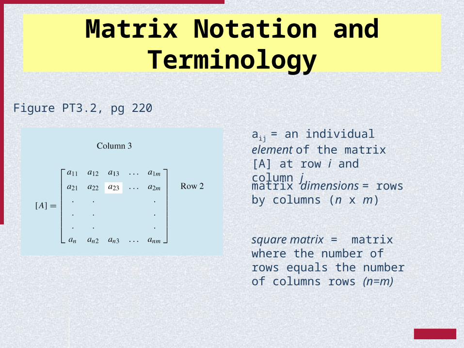
Figure PT3.2, pg 220

aij = an individual element of the matrix [A] at row i and column j

matrix dimensions = rows by columns (n x m)

square matrix = matrix where the number of rows equals the number of columns rows (n=m)

USC

Special Types of Square Matrices

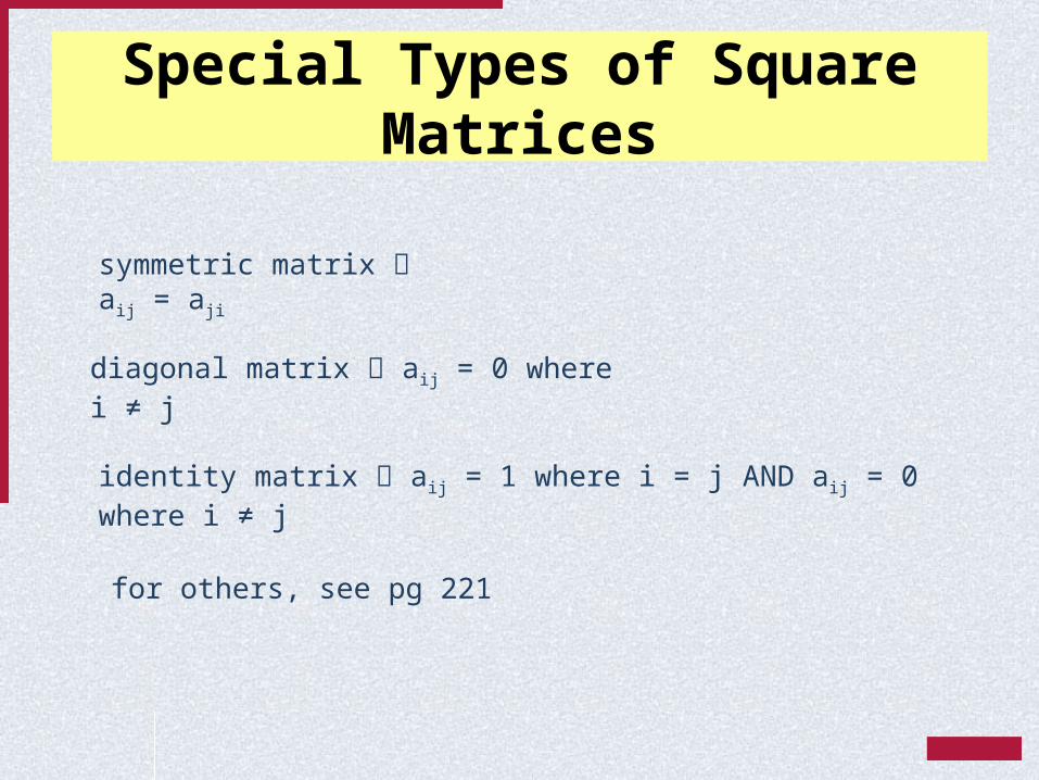
symmetric matrix aij = aji

diagonal matrix aij = 0 where i ≠ j

identity matrix aij = 1 where i = j AND aij = 0 where i ≠ j

for others, see pg 221

USC

Matrix Addition/Subtraction

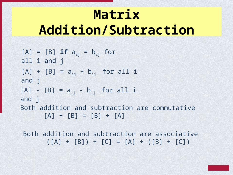
[A] = [B] if aij = bij for all i and j

[A] + [B] = aij + bij for all i and j

[A] - [B] = aij - bij for all i and j

Both addition and subtraction are commutative [A] + [B] = [B] + [A]

Both addition and subtraction are associative ([A] + [B]) + [C] = [A] + ([B] + [C])

USC

Matrix Multiplication by Scalar

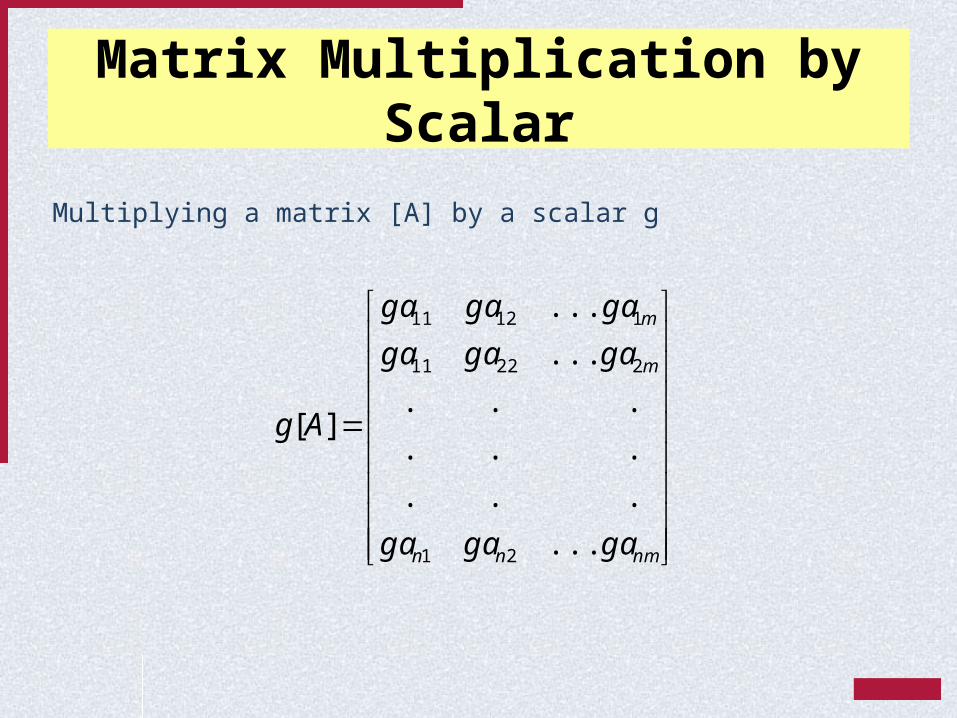
Multiplying a matrix [A] by a scalar g

nmnn

m

m

gagaga

gagaga

gagaga

Ag

...

...

...

...

...

...

][

21

22211

11211

USC

Matrix Multiplication

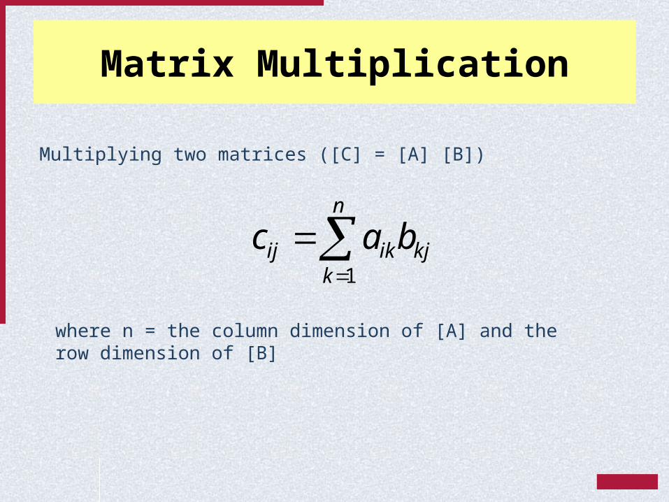
Multiplying two matrices ([C] = [A] [B])

n

kkjikij bac

1

where n = the column dimension of [A] and the row dimension of [B]

USC

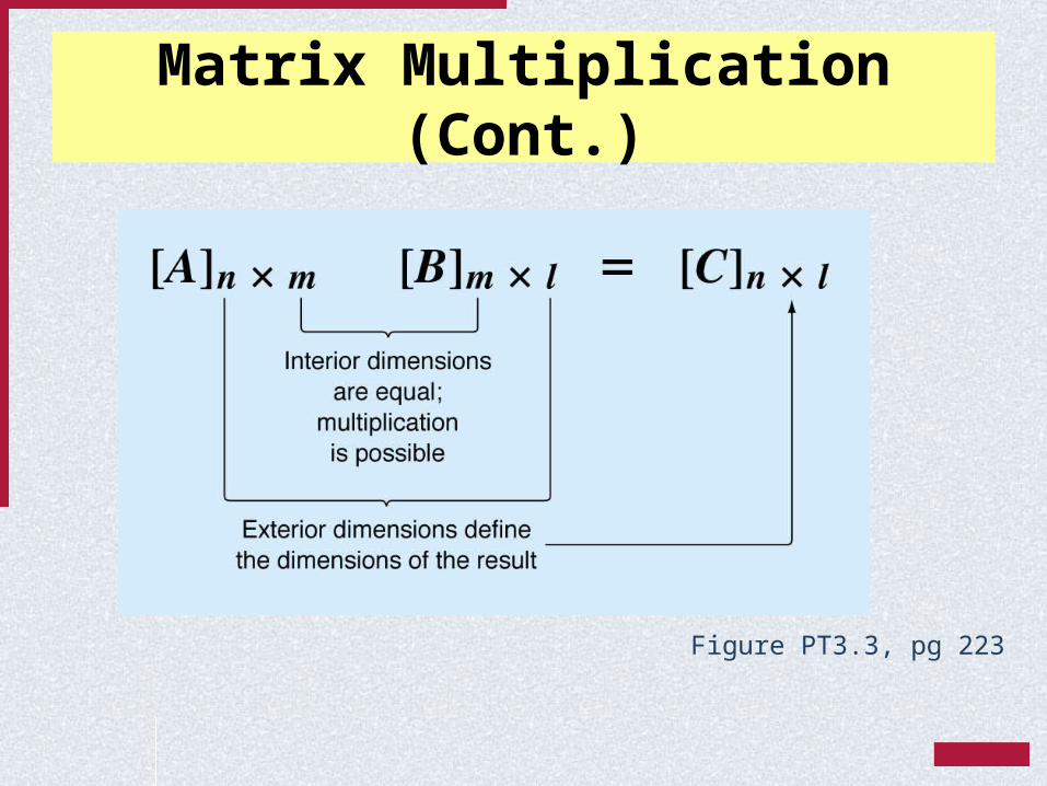
Matrix Multiplication (Cont.)

Figure PT3.3, pg 223

USC

Matrix Multiplication (Cont.)

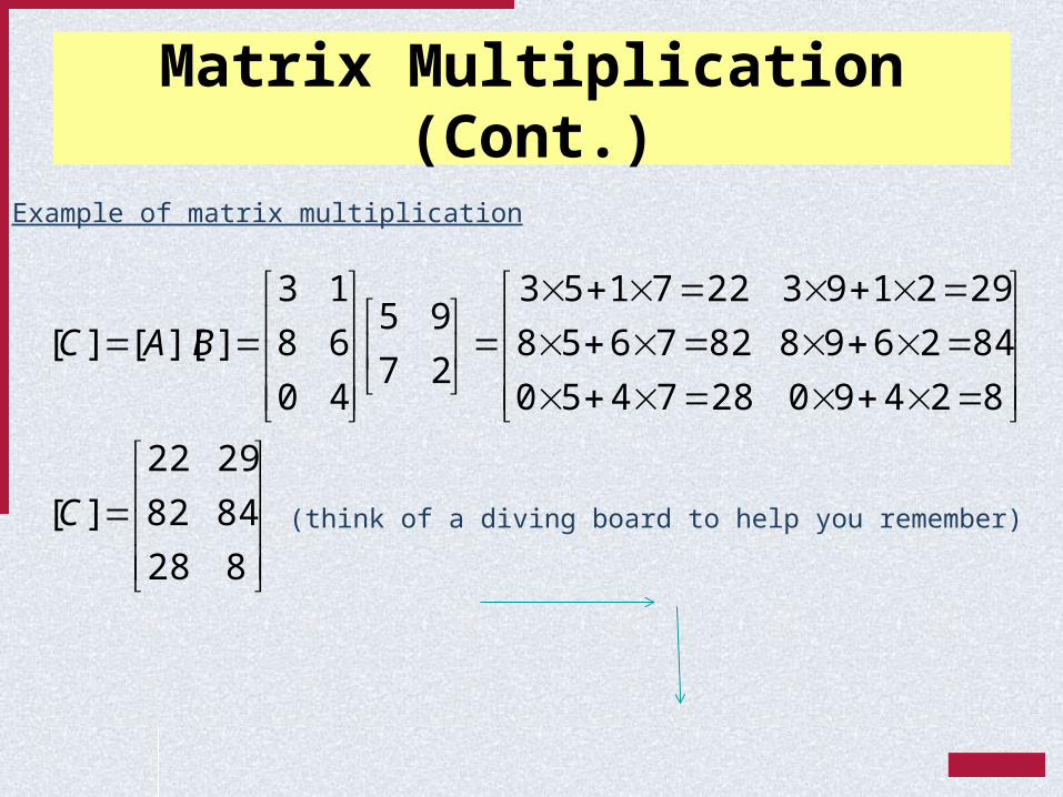
Example of matrix multiplication

828

8482

2922

][

82490287450

842698827658

292193227153

27

95

40

68

13

]][[][

C

BAC

(think of a diving board to help you remember)

USC

Matrix Multiplication (Cont.)

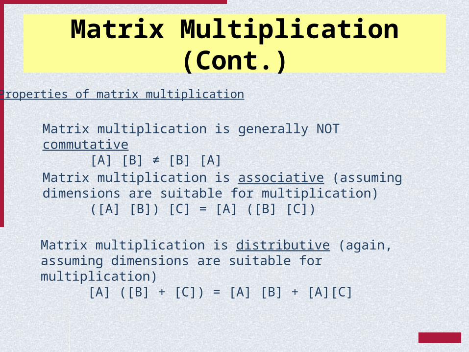
Properties of matrix multiplication

Matrix multiplication is generally NOT commutative [A] [B] ≠ [B] [A]

Matrix multiplication is associative (assuming dimensions are suitable for multiplication)

([A] [B]) [C] = [A] ([B] [C])

Matrix multiplication is distributive (again, assuming dimensions are suitable for multiplication)

[A] ([B] + [C]) = [A] [B] + [A][C]

USC

Matrix Division

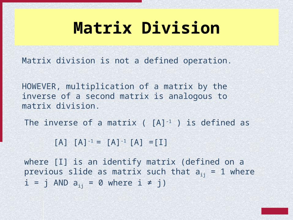
Matrix division is not a defined operation.

The inverse of a matrix ( [A]-1 ) is defined as

[A] [A]-1 = [A]-1 [A] =[I]

where [I] is an identify matrix (defined on a previous slide as matrix such that aij = 1 where i = j AND aij = 0 where i ≠ j)

HOWEVER, multiplication of a matrix by the inverse of a second matrix is analogous to matrix division.

USC

Matrix Inverse

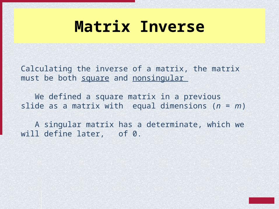
Calculating the inverse of a matrix, the matrix must be both square and nonsingular

We defined a square matrix in a previous slide as a matrix with equal dimensions (n = m)

A singular matrix has a determinate, which we will define later, of 0.

USC

Matrix Inverse (Cont.)

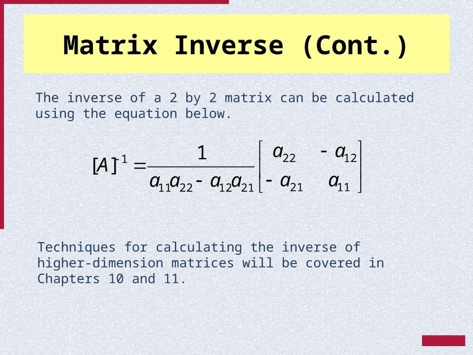
The inverse of a 2 by 2 matrix can be calculated using the equation below.

1121

1222

21122211

1 1][

aa

aa

aaaaA

Techniques for calculating the inverse of higher-dimension matrices will be covered in Chapters 10 and 11.

USC

Matrix Transpose

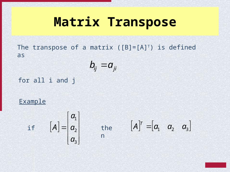
The transpose of a matrix ([B]=[A]T) is defined as

jiij ab for all i and j

Example

3

2

1

a

a

a

A 321 aaaA T if then

USC

Systems of Linear Equations

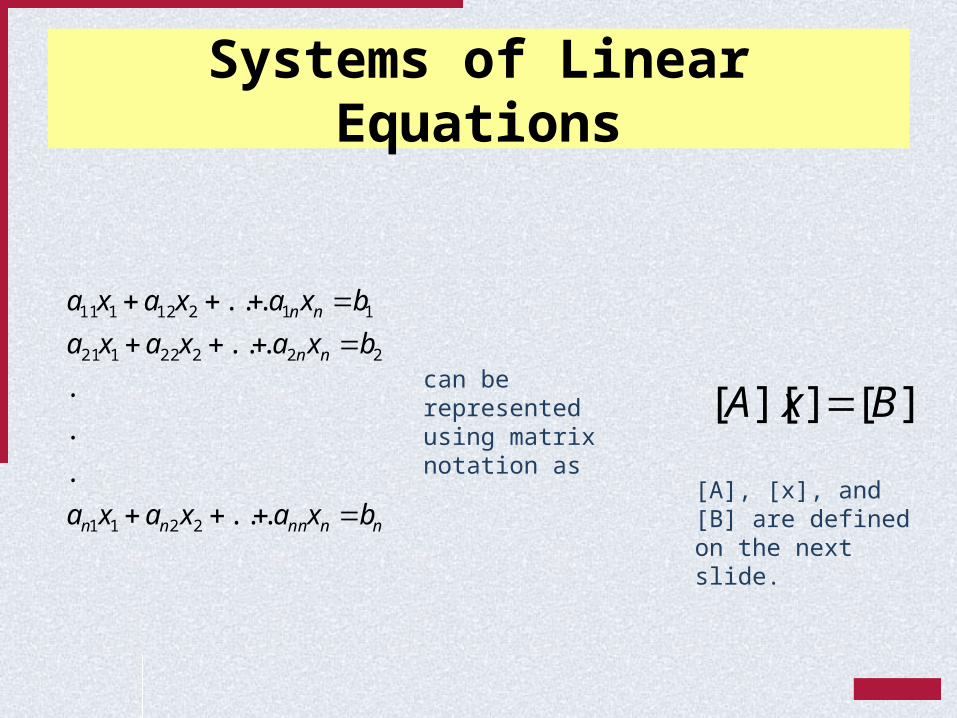
nnnnnn

nn

nn

bxaxaxa

bxaxaxa

bxaxaxa

...

.

.

.

...

...

2211

22222121

11212111

][]][[ BxA can be represented using matrix notation as

[A], [x], and [B] are defined on the next slide.

USC

Matrix Operation Rules (Cont.)

nnnnnn

n

n

b

b

b

x

x

x

aaa

aaa

aaa

.

.

.

.

.

.

...

.

.

.

...

...

2

1

2

1

21

22221

11211

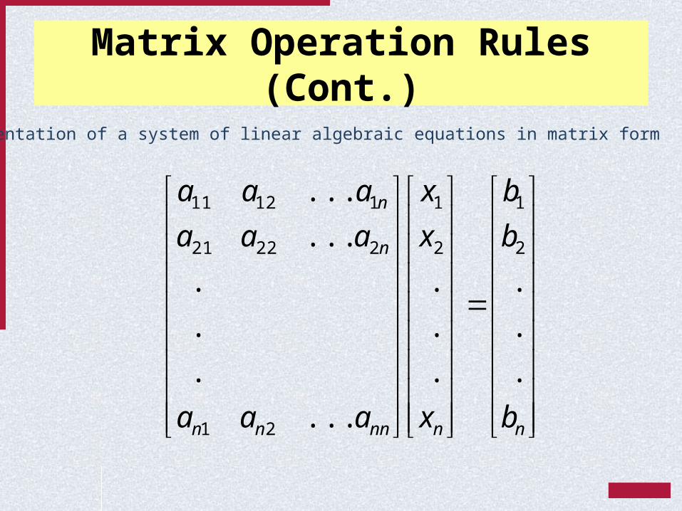
representation of a system of linear algebraic equations in matrix form

USC

Matrix Operation Rules (Cont.)

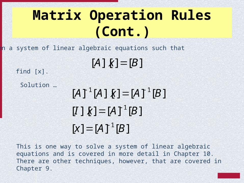
Given a system of linear algebraic equations such that

][]][[ BxA find [x].

][][][

][][]][[

][][]][[][

1

1

11

BAx

BAxI

BAxAA

This is one way to solve a system of linear algebraic equations and is covered in more detail in Chapter 10. There are other techniques, however, that are covered in Chapter 9.

Solution …

USC

Chapter 9

USC

Linear Algebraic EquationsPart 3

An equation of the form ax+by+c=0 or equivalently ax+by=-c is called a linear equation in x and y variables.

ax+by+cz=d is a linear equation in three variables, x, y, and z.

Thus, a linear equation in n variables is

a1x1+a2x2+ … +anxn = b

A solution of such an equation consists of real numbers c1, c2, c3, … , cn. If you need to work more than one linear equations, a system of linear equations must be solved simultaneously.

USC

Noncomputer Methods for Solving Systems of Equations

For small number of equations (n ≤ 3) linear equations can be solved readily by simple techniques such as “method of elimination.”

Linear algebra provides the tools to solve such systems of linear equations.

Nowadays, easy access to computers makes the solution of large sets of linear algebraic equations possible and practical.

USC

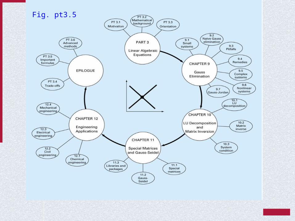
Fig. pt3.5

USC

Gauss EliminationChapter 9

Solving Small Numbers of Equations There are many ways to solve a system of

linear equations: Graphical method Cramer’s rule Method of elimination Computer methods

For n ≤ 3

USC

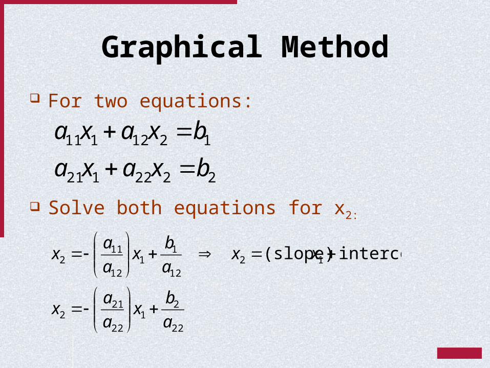
Graphical Method

For two equations:

Solve both equations for x2:

2222121

1212111

bxaxa

bxaxa

22

21

22

212

1212

11

12

112 intercept(slope)

a

bx

a

ax

xxa

bx

a

ax

USC

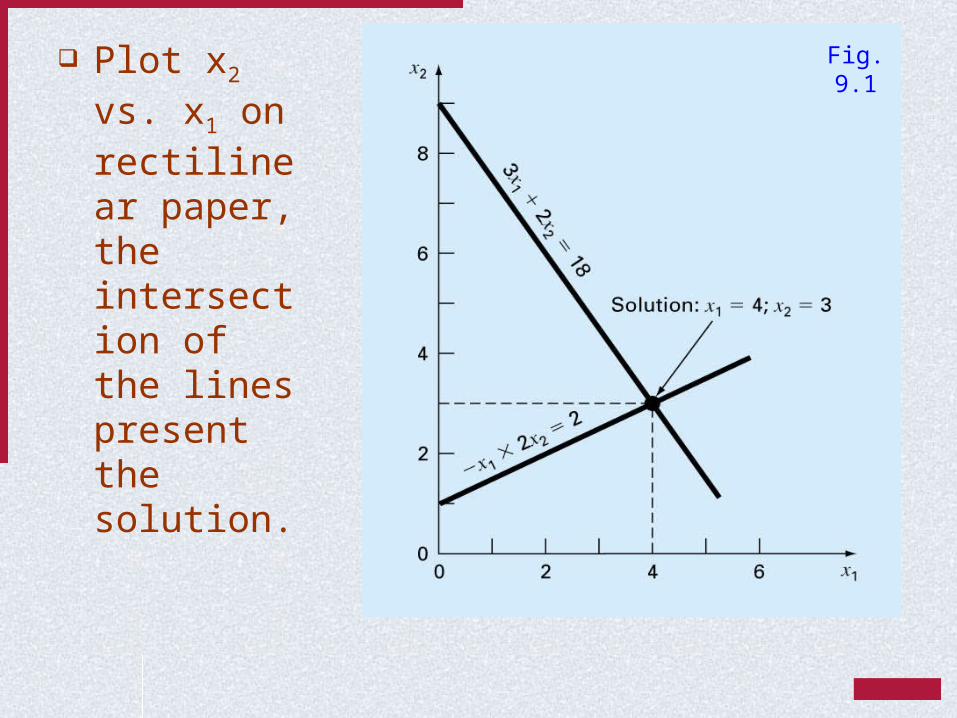
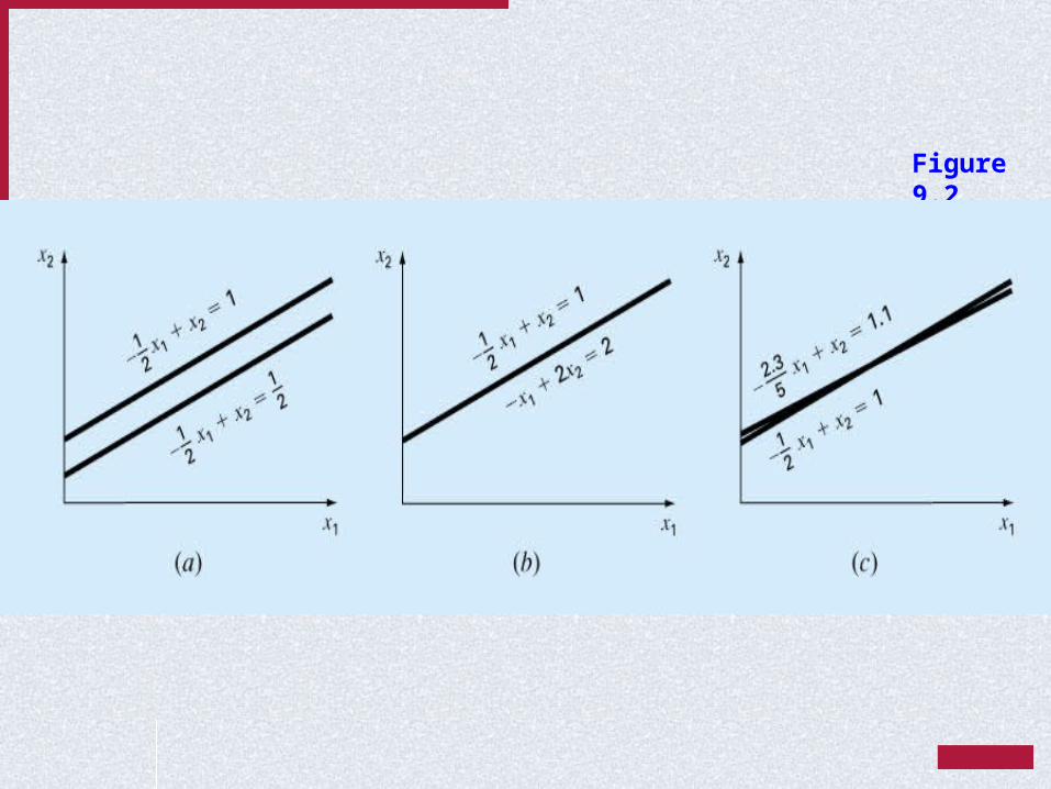
Plot x2 vs. x1 on rectilinear paper, the intersection of the lines present the solution.

Fig. 9.1

USC

Figure 9.2

USC

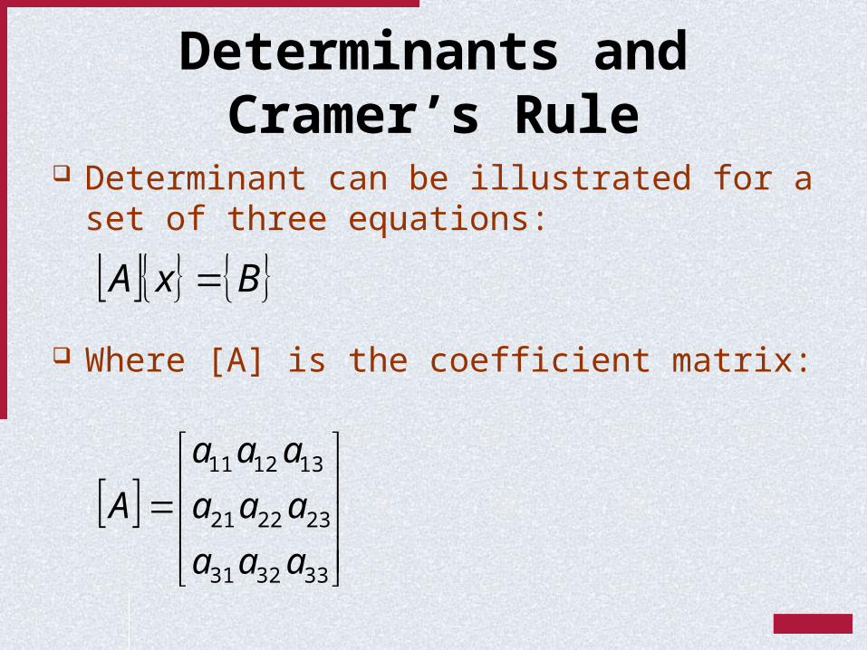
Determinants and Cramer’s Rule

Determinant can be illustrated for a set of three equations:

Where [A] is the coefficient matrix:

BxA

333231

232221

131211

aaa

aaa

aaa

A

USC

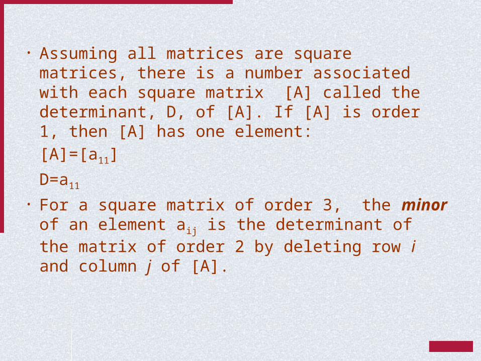
• Assuming all matrices are square matrices, there is a number associated with each square matrix [A] called the determinant, D, of [A]. If [A] is order 1, then [A] has one element:

[A]=[a11]

D=a11

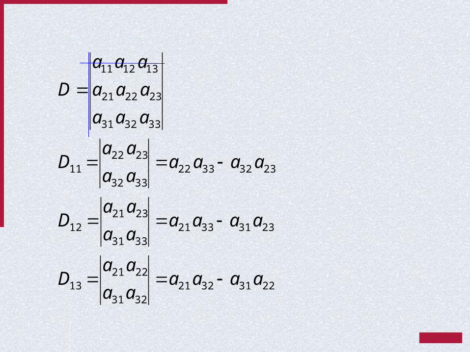
• For a square matrix of order 3, the minor of an element aij is the determinant of the matrix of order 2 by deleting row i and column j of [A].

USC

223132213231

222113

233133213331

232112

233233223332

232211

333231

232221

131211

aaaaaa

aaD

aaaaaa

aaD

aaaaaa

aaD

aaa

aaa

aaa

D

USC

D

aab

aab

aab

x 33323

23222

13121

1

3231

222113

3331

232112

3332

232211 aa

aaa

aa

aaa

aa

aaaD

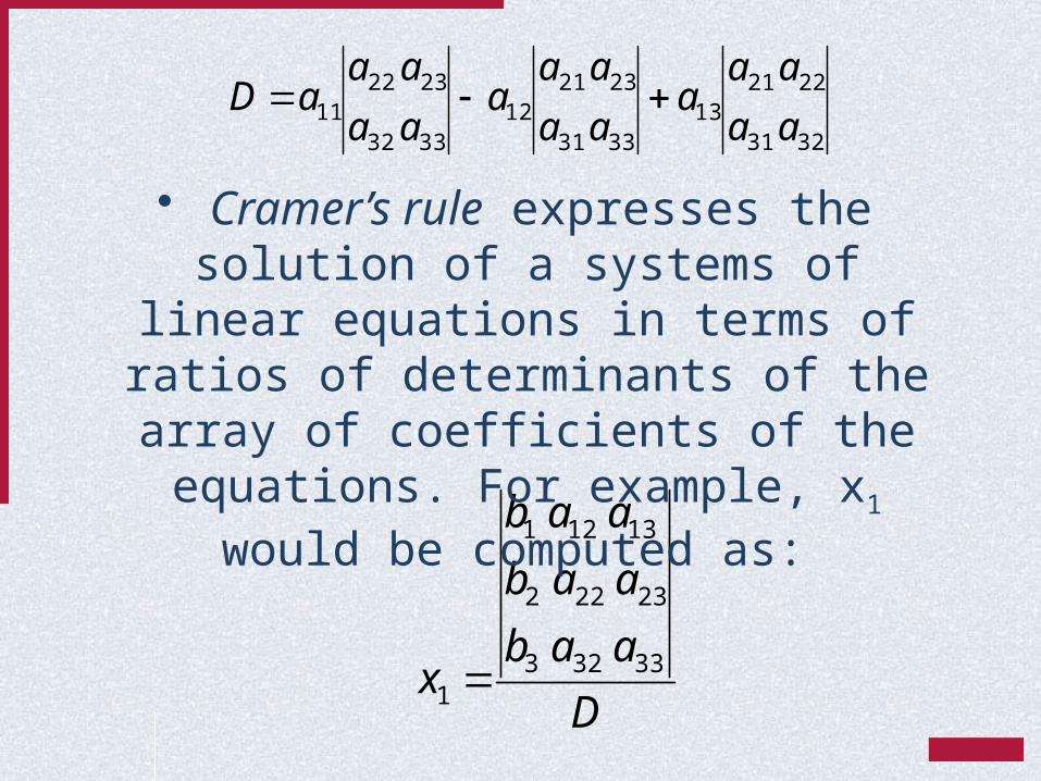
• Cramer’s rule expresses the solution of a systems of linear equations in terms of ratios of determinants of the array of coefficients of

the equations. For example, x1 would be computed as:

USC

Method of Elimination

The basic strategy is to successively solve one of the equations of the set for one of the unknowns and to eliminate that variable from the remaining equations by substitution.

The elimination of unknowns can be extended to systems with more than two or three equations; however, the method becomes extremely tedious to solve by hand.

USC

Naive Gauss Elimination

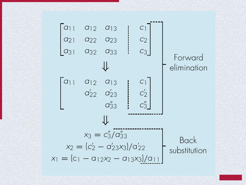
Extension of method of elimination to large sets of equations by developing a systematic scheme or algorithm to eliminate unknowns and to back substitute.

As in the case of the solution of two equations, the technique for n equations consists of two phases: Forward elimination of unknowns Back substitution

USC

USC

Pitfalls of Elimination Methods

Division by zero. It is possible that during both elimination and back-substitution phases a division by zero can occur.

Round-off errors. Ill-conditioned systems. Systems where small changes

in coefficients result in large changes in the solution. Alternatively, it happens when two or more equations are nearly identical, resulting a wide ranges of answers to approximately satisfy the equations. Since round off errors can induce small changes in the coefficients, these changes can lead to large solution errors.

USC

Singular systems. When two equations are identical, we would loose one degree of freedom and be dealing with the impossible case of n-1 equations for n unknowns. For large sets of equations, it may not be obvious however. The fact that the determinant of a singular system is zero can be used and tested by computer algorithm after the elimination stage. If a zero diagonal element is created, calculation is terminated.

USC

Techniques for Improving Solutions

• Use of more significant figures.• Pivoting. If a pivot element is zero,

normalization step leads to division by zero. The same problem may arise, when the pivot element is close to zero. Problem can be avoided:– Partial pivoting. Switching the rows so that the

largest element is the pivot element.– Complete pivoting. Searching for the largest element

in all rows and columns then switching.

USC

Gauss-Jordan

It is a variation of Gauss elimination. The major differences are: When an unknown is eliminated, it is eliminated

from all other equations rather than just the subsequent ones.

All rows are normalized by dividing them by their pivot elements.

Elimination step results in an identity matrix. Consequently, it is not necessary to employ back

substitution to obtain solution.

USC

Chapter 10

USC

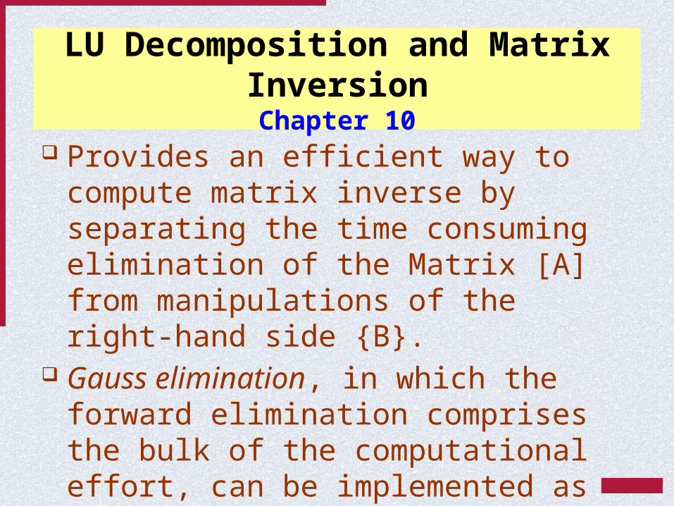
LU Decomposition and Matrix InversionChapter 10

Provides an efficient way to compute matrix inverse by separating the time consuming elimination of the Matrix [A] from manipulations of the right-hand side {B}.

Gauss elimination, in which the forward elimination comprises the bulk of the computational effort, can be implemented as an LU decomposition.

USC

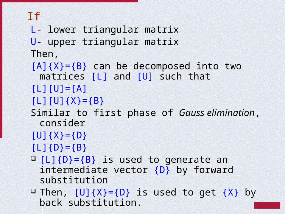
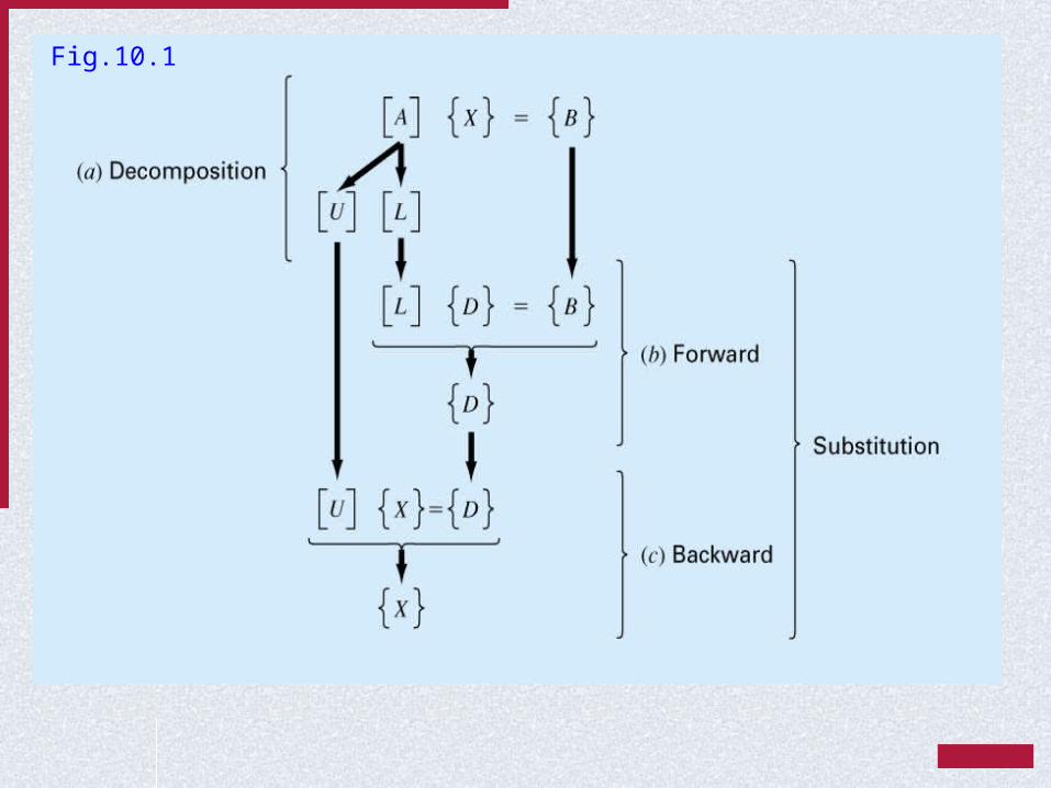
IfL- lower triangular matrixU- upper triangular matrixThen,[A]{X}={B} can be decomposed into two matrices [L] and

[U] such that[L][U]=[A][L][U]{X}={B}Similar to first phase of Gauss elimination, consider[U]{X}={D}[L]{D}={B} [L]{D}={B} is used to generate an intermediate vector

{D} by forward substitution Then, [U]{X}={D} is used to get {X} by back substitution.

USC

Fig.10.1

USC

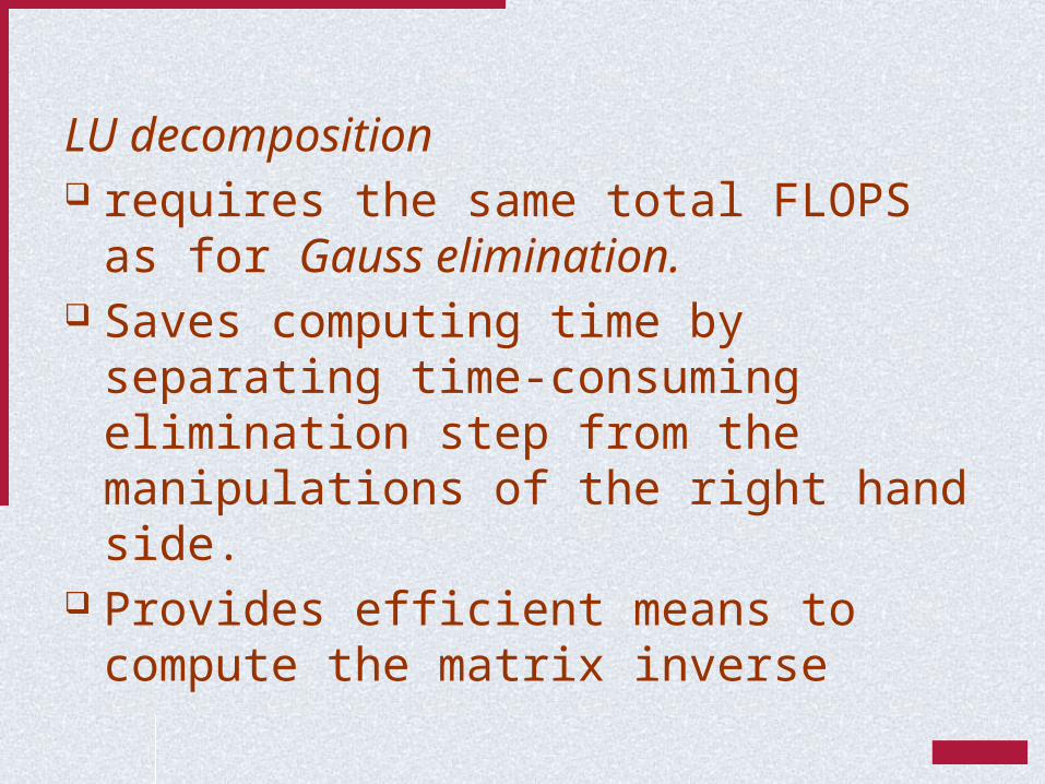
LU decomposition requires the same total FLOPS as for Gauss

elimination. Saves computing time by separating time-

consuming elimination step from the manipulations of the right hand side.

Provides efficient means to compute the matrix inverse

USC

The Matrix Inverse

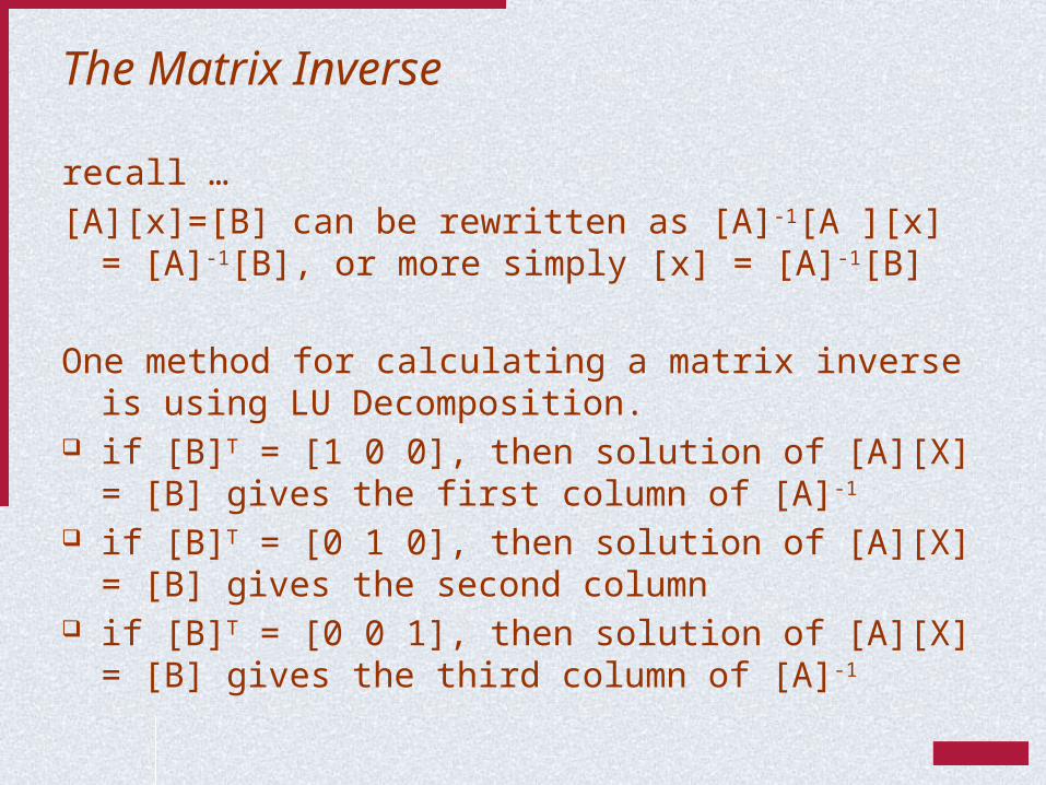
recall …

[A][x]=[B] can be rewritten as [A]-1[A ][x] = [A]-1[B], or more simply [x] = [A]-1[B]

One method for calculating a matrix inverse is using LU Decomposition.

if [B]T = [1 0 0], then solution of [A][X] = [B] gives the first column of [A]-1

if [B]T = [0 1 0], then solution of [A][X] = [B] gives the second column

if [B]T = [0 0 1], then solution of [A][X] = [B] gives the third column of [A]-1