Embed Size (px)
Citation preview

http://www.elsolucionario.blogspot.com
LIBROS UNIVERISTARIOS Y SOLUCIONARIOS DE MUCHOS DE ESTOS LIBROS
LOS SOLUCIONARIOS CONTIENEN TODOS LOS EJERCICIOS DEL LIBRORESUELTOS Y EXPLICADOSDE FORMA CLARA
VISITANOS PARADESARGALOS GRATIS.

CHAPTER 2
2.1 IF x < 10 THEN
IF x < 5 THEN
x = 5
ELSE
PRINT x
END IF
ELSE
DO
IF x < 50 EXIT
x = x - 5
END DO
END IF
2.2Step 1: StartStep 2: Initialize sum and count to zeroStep 3: Examine top card.Step 4: If it says “end of data” proceed to step 9; otherwise, proceed to next step.Step 5: Add value from top card to sum.Step 6: Increase count by 1.Step 7: Discard top cardStep 8: Return to Step 3.Step 9: Is the count greater than zero?
If yes, proceed to step 10.If no, proceed to step 11.
Step 10: Calculate average = sum/countStep 11: End
2.3 start
sum = 0count = 0
INPUT
value
value =
“end of data”
value =
“end of data”
sum = sum + valuecount = count + 1
T
F
count > 0
average = sum/count
end
T
F

2.4Students could implement the subprogram in any number of languages. The followingFortran 90 program is one example. It should be noted that the availability of complexvariables in Fortran 90, would allow this subroutine to be made even more concise.However, we did not exploit this feature, in order to make the code more compatible withVisual BASIC, MATLAB, etc.
PROGRAM RootfindIMPLICIT NONEINTEGER::ierREAL::a, b, c, r1, i1, r2, i2DATA a,b,c/1.,5.,2./CALL Roots(a, b, c, ier, r1, i1, r2, i2)IF (ier .EQ. 0) THEN PRINT *, r1,i1," i" PRINT *, r2,i2," i"ELSE PRINT *, "No roots"END IFEND
SUBROUTINE Roots(a, b, c, ier, r1, i1, r2, i2)IMPLICIT NONEINTEGER::ierREAL::a, b, c, d, r1, i1, r2, i2r1=0.r2=0.i1=0.i2=0. IF (a .EQ. 0.) THEN IF (b <> 0) THEN r1 = -c/b ELSE ier = 1 END IFELSE d = b**2 - 4.*a*c IF (d >= 0) THEN r1 = (-b + SQRT(d))/(2*a) r2 = (-b - SQRT(d))/(2*a) ELSE r1 = -b/(2*a) r2 = r1 i1 = SQRT(ABS(d))/(2*a) i2 = -i1 END IFEND IFEND
The answers for the 3 test cases are: (a) −0.438, -4.56; (b) 0.5; (c) −1.25 + 2.33i; −1.25 −2.33i.
Several features of this subroutine bear mention:
• The subroutine does not involve input or output. Rather, information is passed in and outvia the arguments. This is often the preferred style, because the I/O is left to thediscretion of the programmer within the calling program.
• Note that an error code is passed (IER = 1) for the case where no roots are possible.

2.5 The development of the algorithm hinges on recognizing that the series approximation of thesine can be represented concisely by the summation,
x
i
i
i
n 2 1
1 2 1
−
= −∑( )!
where i = the order of the approximation. The following algorithm implements thissummation:
Step 1: StartStep 2: Input value to be evaluated x and maximum order nStep 3: Set order (i) equal to oneStep 4: Set accumulator for approximation (approx) to zeroStep 5: Set accumulator for factorial product (fact) equal to oneStep 6: Calculate true value of sin(x)Step 7: If order is greater than n then proceed to step 13 Otherwise, proceed to next stepStep 8: Calculate the approximation with the formula
approx approx ( 1)x
factor
i-12i-1
= + −
Step 9: Determine the error
100%true
approxtrue%error
−=
Step 10: Increment the order by oneStep 11: Determine the factorial for the next iteration
factor factor (2 i 2) (2 i 1)= • • − • • −Step 12: Return to step 7Step 13: End

2.6
start
INPUTx, n
i > n
end
i = 1
true = sin(x)approx = 0
factor = 1
approx approxx
factor
ii -
= + -( 1) - 12 1
errortrue approx
true100=
−%
OUTPUT
i,approx,error
i = i + 1
F
T
factor=factor(2i-2)(2i-1)
Pseudocode:
SUBROUTINE Sincomp(n,x)
i = 1
true = SIN(x)
approx = 0
factor = 1
DO
IF i > n EXIT
approx = approx + (-1)i-1•x2•i-1 / factor
error = Abs(true - approx) / true) * 100
PRINT i, true, approx, error
i = i + 1
factor = factor•(2•i-2)•(2•i-1)END DO
END

2.7 The following Fortran 90 code was developed based on the pseudocode from Prob. 2.6:
PROGRAM SeriesIMPLICIT NONEINTEGER::nREAL::xn = 15x = 1.5CALL Sincomp(n,x)END
SUBROUTINE Sincomp(n,x)IMPLICIT NONEINTEGER::n,i,facREAL::x,tru,approx,eri = 1tru = SIN(x)approx = 0.fac = 1PRINT *, " order true approx error"DO IF (i > n) EXIT approx = approx + (-1) ** (i-1) * x ** (2*i - 1) / fac er = ABS(tru - approx) / tru) * 100 PRINT *, i, tru, approx, er i = i + 1 fac = fac * (2*i-2) * (2*i-1)END DOEND
OUTPUT: order true approx error 1 0.9974950 1.500000 -50.37669 2 0.9974950 0.9375000 6.014566 3 0.9974950 1.000781 -0.3294555 4 0.9974950 0.9973912 1.0403229E-02 5 0.9974950 0.9974971 -2.1511559E-04 6 0.9974950 0.9974950 0.0000000E+00 7 0.9974950 0.9974951 -1.1950866E-05 8 0.9974950 0.9974949 1.1950866E-05 9 0.9974950 0.9974915 3.5255053E-04 10 0.9974950 0.9974713 2.3782223E-03 11 0.9974950 0.9974671 2.7965026E-03 12 0.9974950 0.9974541 4.0991469E-03 13 0.9974950 0.9974663 2.8801586E-03 14 0.9974950 0.9974280 6.7163869E-03 15 0.9974950 0.9973251 1.7035959E-02Press any key to continue
The errors can be plotted versus the number of terms:
1.E-05
1.E-04
1.E-03
1.E-02
1.E-01
1.E+00
1.E+01
1.E+02
0 5 10 15
error

Interpretation: The absolute percent relative error drops until at n = 6, it actually yields aperfect result (pure luck!). Beyond, n = 8, the errors starts to grow. This occurs because ofround-off error, which will be discussed in Chap. 3.
2.8 AQ = 442/5 = 88.4AH = 548/6 = 91.33
without final
AG =30(88.4) + 30(91.33)
30 + 30= 89 8667.
with final
AG =30(88.4) + 30(91.33) + 40(91)
30 + 30= 90 32.
The following pseudocode provides an algorithm to program this problem. Notice that theinput of the quizzes and homeworks is done with logical loops that terminate when the userenters a negative grade:
INPUT number, nameINPUT WQ, WH, WFnq = 0sumq = 0DO INPUT quiz (enter negative to signal end of quizzes) IF quiz < 0 EXIT nq = nq + 1 sumq = sumq + quizEND DOAQ = sumq / nqPRINT AQnh = 0sumh = 0PRINT "homeworks"DO INPUT homework (enter negative to signal end of homeworks) IF homework < 0 EXIT nh = nh + 1 sumh = sumh + homeworkEND DOAH = sumh / nhPRINT "Is there a final grade (y or n)"INPUT answerIF answer = "y" THEN INPUT FE AG = (WQ * AQ + WH * AH + WF * FE) / (WQ + WH + WF)ELSE AG = (WQ * AQ + WH * AH) / (WQ + WH)END IFPRINT number, name$, AGEND
2.9

n F
0 $100,000.00
1 $108,000.00
2 $116,640.00
3 $125,971.20
4 $136,048.90
5 $146,932.81
24 $634,118.07
25 $684,847.52
2.10 Programs vary, but results are
Bismarck = −10.842 t = 0 to 59 Yuma = 33.040 t = 180 to 242
2.11 n A1 40,250.002 21,529.073 15,329.194 12,259.295 10,441.04
2.12
Step v(12) εt (%)2 49.96 -5.21 48.70 -2.60.5 48.09 -1.3
Error is halved when step is halved
2.13
Fortran 90 VBA

Subroutine BubbleFor(n, b)
Implicit None
!sorts an array in ascending!order using the bubble sort
Integer(4)::m, i, nLogical::switchReal::a(n),b(n),dum
m = n - 1Do switch = .False. Do i = 1, m If (b(i) > b(i + 1)) Then dum = b(i) b(i) = b(i + 1) b(i + 1) = dum switch = .True. End If End Do If (switch == .False.) Exit m = m - 1End Do
End
Option Explicit
Sub Bubble(n, b)
'sorts an array in ascending'order using the bubble sort
Dim m As Integer, i As IntegerDim switch As BooleanDim dum As Single
m = n - 1Do switch = False For i = 1 To m If b(i) > b(i + 1) Then dum = b(i) b(i) = b(i + 1) b(i + 1) = dum switch = True End If Next i If switch = False Then Exit Do m = m - 1Loop
End Sub
2.14 Here is a flowchart for the algorithm:
Function Vol(R, d)
pi = 3.141593
d < R
d < 3 * R
V1 = pi * R^3 / 3
V2 = pi * R^2 (d – R)
Vol = V1 + V2
Vol =
“Overtop”
End Function
Vol = pi * d^3 / 3
Here is a program in VBA:
Option Explicit
Function Vol(R, d)

Dim V1 As Single, v2 As Single, pi As Single
pi = 4 * Atn(1)
If d < R Then Vol = pi * d ^ 3 / 3ElseIf d <= 3 * R Then V1 = pi * R ^ 3 / 3 v2 = pi * R ^ 2 * (d - R) Vol = V1 + v2Else Vol = "overtop"End If
End Function
The results are
R d Volume1 0.3 0.0282741 0.8 0.5361651 1 1.0471981 2.2 4.8171091 3 7.3303831 3.1 overtop
2.15 Here is a flowchart for the algorithm:
Function Polar(x, y)
22 yxr +=
x < 0
y > 0y > 0
πθ +
= −
x
y1tan
πθ −
= −
x
y1tan πθ −
= −
x
y1tanθ = 0
2
πθ −=
y < 02
πθ =
θ = π
y < 0
πθ 180=Polarπ
θ 180=Polar
End Polar
π = 3.141593
T
T
T
T
T
F
F
F
F
And here is a VBA function procedure to implement it:
Option Explicit
Function Polar(x, y)

Dim th As Single, r As SingleConst pi As Single = 3.141593
r = Sqr(x ^ 2 + y ^ 2)
If x < 0 Then If y > 0 Then th = Atn(y / x) + pi ElseIf y < 0 Then th = Atn(y / x) - pi Else th = pi End IfElse If y > 0 Then th = pi / 2 ElseIf y < 0 Then th = -pi / 2 Else th = 0 End IfEnd If
Polar = th * 180 / pi
End Function
The results are:
x y θ1 1 901 -1 -901 0 0-1 1 135-1 -1 -135-1 0 1800 1 900 -1 -900 0 0


4.18 f(x) = x-1-1/2*sin(x)f '(x) = 1-1/2*cos(x)f ''(x) = 1/2*sin(x)f '''(x) = 1/2*cos(x)f IV(x) = -1/2*sin(x)
Using the Taylor Series Expansion (Equation 4.5 in the book), we obtain the following1st, 2nd, 3rd, and 4th Order Taylor Series functions shown below in the Matlab program-f1, f2, f4. Note the 2nd and 3rd Order Taylor Series functions are the same.
From the plots below, we see that the answer is the 4 th Order Taylor Series expansion .
x=0:0.001:3.2;
f=x-1-0.5*sin(x);subplot(2,2,1);plot(x,f);grid;title('f(x)=x-1-0.5*sin(x)');hold on
f1=x-1.5;e1=abs(f-f1); %Calculates the absolute value of thedifference/errorsubplot(2,2,2);plot(x,e1);grid;title('1st Order Taylor Series Error');
f2=x-1.5+0.25.*((x-0.5*pi).^2);e2=abs(f-f2);subplot(2,2,3);plot(x,e2);grid;title('2nd/3rd Order Taylor Series Error');
f4=x-1.5+0.25.*((x-0.5*pi).^2)-(1/48)*((x-0.5*pi).^4);e4=abs(f4-f);subplot(2,2,4);plot(x,e4);grid;title('4th Order Taylor Series Error');hold off

0 1 2 3 4-1
0
1
2
3f(x )=x -1-0.5*s in(x )
0 1 2 3 40
0.2
0.4
0.6
0.81s t Order Tay lor S eries E rror
0 1 2 3 40
0.05
0.1
0.15
0.22nd/3rd Order Tay lor S eries E rror
0 1 2 3 40
0.005
0.01
0.0154th Order Tay lor S eries E rror
4.19 EXCEL WORKSHEET AND PLOTS
First Derivative Approximations Compared to Theoretical
-4.0
-2.0
0.0
2.0
4.0
6.0
8.0
10.0
12.0
14.0
-2.5 -2.0 -1.5 -1.0 -0.5 0.0 0.5 1.0 1.5 2.0 2.5
x-values
f'(x
)
Theoretical
Backward
Centered
Forward

Approximations of the 2nd Derivative
-15.0
-10.0
-5.0
0.0
5.0
10.0
15.0
-2.5 -2.0 -1.5 -1.0 -0.5 0.0 0.5 1.0 1.5 2.0 2.5
x-values
f''(x)
f''(x)-Theory
f''(x)-Backward
f''(x)-Centered
f''(x)-Forward
x f(x) f(x-1) f(x+1) f(x-2) f(x+2) f''(x)-
Theory
f''(x)-
Back
f''(x)-Cent f''(x)-
Forw-2.000 0.000 -2.891 2.141 3.625 3.625 -12.000 150.500 -12.000 -10.500
-1.750 2.141 0.000 3.625 -2.891 4.547 -10.500 -12.000 -10.500 -9.000
-1.500 3.625 2.141 4.547 0.000 5.000 -9.000 -10.500 -9.000 -7.500
-1.250 4.547 3.625 5.000 2.141 5.078 -7.500 -9.000 -7.500 -6.000
-1.000 5.000 4.547 5.078 3.625 4.875 -6.000 -7.500 -6.000 -4.500
-0.750 5.078 5.000 4.875 4.547 4.484 -4.500 -6.000 -4.500 -3.000
-0.500 4.875 5.078 4.484 5.000 4.000 -3.000 -4.500 -3.000 -1.500
-0.250 4.484 4.875 4.000 5.078 3.516 -1.500 -3.000 -1.500 0.000
0.000 4.000 4.484 3.516 4.875 3.125 0.000 -1.500 0.000 1.500
0.250 3.516 4.000 3.125 4.484 2.922 1.500 0.000 1.500 3.000
0.500 3.125 3.516 2.922 4.000 3.000 3.000 1.500 3.000 4.500
0.750 2.922 3.125 3.000 3.516 3.453 4.500 3.000 4.500 6.000
1.000 3.000 2.922 3.453 3.125 4.375 6.000 4.500 6.000 7.500
1.250 3.453 3.000 4.375 2.922 5.859 7.500 6.000 7.500 9.000
1.500 4.375 3.453 5.859 3.000 8.000 9.000 7.500 9.000 10.500
1.750 5.859 4.375 8.000 3.453 10.891 10.500 9.000 10.500 12.000
2.000 8.000 5.859 10.891 4.375 14.625 12.000 10.500 12.000 13.500
x f(x) f(x-1) f(x+1) f'(x)-Theory f'(x)-Back f'(x)-Cent f'(x)-Forw
-2.000 0.000 -2.891 2.141 10.000 11.563 10.063 8.563
-1.750 2.141 0.000 3.625 7.188 8.563 7.250 5.938
-1.500 3.625 2.141 4.547 4.750 5.938 4.813 3.688
-1.250 4.547 3.625 5.000 2.688 3.688 2.750 1.813
-1.000 5.000 4.547 5.078 1.000 1.813 1.063 0.313
-0.750 5.078 5.000 4.875 -0.313 0.313 -0.250 -0.813
-0.500 4.875 5.078 4.484 -1.250 -0.813 -1.188 -1.563
-0.250 4.484 4.875 4.000 -1.813 -1.563 -1.750 -1.938
0.000 4.000 4.484 3.516 -2.000 -1.938 -1.938 -1.938
0.250 3.516 4.000 3.125 -1.813 -1.938 -1.750 -1.563
0.500 3.125 3.516 2.922 -1.250 -1.563 -1.188 -0.813
0.750 2.922 3.125 3.000 -0.313 -0.813 -0.250 0.313
1.000 3.000 2.922 3.453 1.000 0.313 1.063 1.813
1.250 3.453 3.000 4.375 2.688 1.813 2.750 3.688
1.500 4.375 3.453 5.859 4.750 3.688 4.813 5.938
1.750 5.859 4.375 8.000 7.188 5.938 7.250 8.563
2.000 8.000 5.859 10.891 10.000 8.563 10.063 11.563


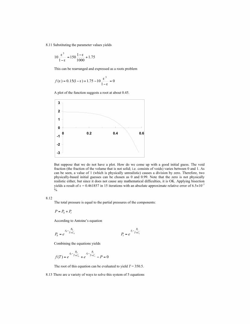
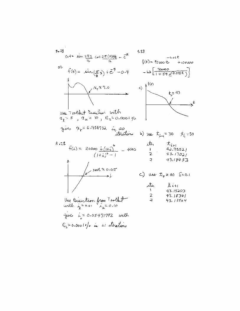
8.11 Substituting the parameter values yields
75.11000
1150
110
3
+−
=−
εε
ε
This can be rearranged and expressed as a roots problem
01
1075.1)1(15.0)(3
=−
−+−=ε
εεεf
A plot of the function suggests a root at about 0.45.
-3
-2
-1
0
1
2
3
0 0.2 0.4 0.6
But suppose that we do not have a plot. How do we come up with a good initial guess. The voidfraction (the fraction of the volume that is not solid; i.e. consists of voids) varies between 0 and 1. Ascan be seen, a value of 1 (which is physically unrealistic) causes a division by zero. Therefore, twophysically-based initial guesses can be chosen as 0 and 0.99. Note that the zero is not physicallyrealistic either, but since it does not cause any mathematical difficulties, it is OK. Applying bisection
yields a result of ε = 0.461857 in 15 iterations with an absolute approximate relative error of 6.5×10⁻³
%
8.12 The total pressure is equal to the partial pressures of the components:
tb PPP +=
According to Antoine’s equation
b
bb
CT
BA
b eP+
−
= t
tt
CT
BA
t eP+
−
=
Combining the equations yields
0)( =−+= +−
+−
PeeTf t
tt
b
bb
CT
BA
CT
BA
The root of this equation can be evaluated to yield T = 350.5.
8.13 There are a variety of ways to solve this system of 5 equations

][CO
]][HCO[H
2
31
−+
=K (1)
][HCO
]][CO[H
3
23
2 −
−+
=K (2)
]][OH[H= + −wK (3)
][CO][HCO][CO= 2332−− ++Tc (4)
][H][OH+][CO2][HCO=Alk +233 −+ −−− (5)
One way is to combine the equations to produce a single polynomial. Equations 1 and 2 can be solvedfor
1
332
]][HCO[H]CO[H *
K
−+
=][HCO
][H][CO
3
223 −
+− =
K
These results can be substituted into Eq. 4, which can be solved for
TcF032 ]CO[H * = TcF13 ][HCO =−TcF2
23 ][CO =−
where F0, F1, and F2 are the fractions of the total inorganic carbon in carbon dioxide, bicarbonate and
carbonate, respectively, where
2112
2
0][H][H
][H=
KKKF
++ ++
+
211
2
11
][H][H
][H=
KKK
KF
++ ++
+
211
2
212
][H][H=
KKK
KKF
++ ++
Now these equations, along with the Eq. 3 can be substituted into Eq. 5 to give
Alk][H][H+2=0 ++21 −−+ wTT KcFcF
Although it might not be apparent, this result is a fourth-order polynomial in [H+].
( ) ( ) 2+1121
3+1
4+ ]H[Alk]H[Alk]H[ Tw cKKKKKK −−++++
( ) 0]H[2Alk 21+
21121 =−−−+ wTw KKKcKKKKKK
Substituting parameter values gives
010512.2]H[10055.1]H[10012.5]H[10001.2]H[ 31+192+103+34+ =×−×−×−×+ −−−−
This equation can be solved for [H+] = 2.51x10⁻⁷ (pH = 6.6). This value can then be used to compute
8
7
14
1098.31051.2
10][OH −
−
−− ×=
×=

( )( ) ( )
( ) 001.010333304.01031010102.5110102.51
102.51=]COH[
33
3.103.67-3.627-
27-
32* =×=×
+×+×
× −−
−−−
( )( ) ( )
( ) 002.0103666562.01031010102.5110102.51
102.5110=]HCO[ 33
3.103.67-3.627-
-73.6
3 =×=×+×+×
× −−
−−−
−−
( ) ( )( ) M433
3.103.67-3.627-
3.103.623 1033.1103000133.0103
1010102.5110102.51
1010=]CO[ −−−
−−−
−−− ×=×=×
+×+×8.14 The integral can be evaluated as
−+
−=+− ∫ inout
in
out
maxmaxmax
ln11out
in
CCC
CK
kdc
kCk
KC
C
Therefore, the problem amounts to finding the root of
−+
+= inout
in
out
max
out ln1
)( CCC
CK
kF
VCf
Excel solver can be used to find the root:


8.24 %Region from x=8 to x=10x1=[8:.1:10];y1=20*(x1-(x1-5))-15-57;figure (1)plot(x1,y1)grid
%Region from x=7 to x=8x2=[7:.1:8];y2=20*(x2-(x2-5))-57;figure (2)plot(x2,y2)grid
%Region from x=5 to x=7x3=[5:.1:7];y3=20*(x3-(x3-5))-57;figure (3)plot(x3,y3)grid
%Region from x=0 to x=5x4=[0:.1:5];y4=20*x4-57;figure (4)plot(x4,y4)grid
%Region from x=0 to x=10figure (5)plot(x1,y1,x2,y2,x3,y3,x4,y4)gridtitle('shear diagram')
a=[20 -57]roots(a)
a = 20 -57
ans = 2.8500
0 1 2 3 4 5 6 7 8 9 10-60
-40
-20
0
20
40
60s hear diagram

8.25%Region from x=7 to x=8x2=[7:.1:8];y2=-10*(x2.^2-(x2-5).^2)+150+57*x2;figure (2)plot(x2,y2)grid
%Region from x=5 to x=7x3=[5:.1:7];y3=-10*(x3.^2-(x3-5).^2)+57*x3;figure (3)plot(x3,y3)grid
%Region from x=0 to x=5x4=[0:.1:5];y4=-10*(x4.^2)+57*x4;figure (4)plot(x4,y4)grid
%Region from x=0 to x=10figure (5)plot(x1,y1,x2,y2,x3,y3,x4,y4)gridtitle('moment diagram')
a=[-43 250]roots(a)
a = -43 250
ans = 5.8140
0 1 2 3 4 5 6 7 8 9 10-60
-40
-20
0
20
40
60
80
100m om ent diagram

8.26 A Matlab script can be used to determine that the slope equals zero at x = 3.94 m.
%Region from x=8 to x=10x1=[8:.1:10];y1=((-10/3)*(x1.^3-(x1-5).^3))+7.5*(x1-8).^2+150*(x1-7)+(57/2)*x1.^2-238.25;figure (1)plot(x1,y1)grid%Region from x=7 to x=8x2=[7:.1:8];y2=((-10/3)*(x2.^3-(x2-5).^3))+150*(x2-7)+(57/2)*x2.^2-238.25;figure (2)plot(x2,y2)grid%Region from x=5 to x=7x3=[5:.1:7];y3=((-10/3)*(x3.^3-(x3-5).^3))+(57/2)*x3.^2-238.25;figure (3)plot(x3,y3)grid%Region from x=0 to x=5x4=[0:.1:5];y4=((-10/3)*(x4.^3))+(57/2)*x4.^2-238.25;figure (4)plot(x4,y4)grid%Region from x=0 to x=10figure (5)plot(x1,y1,x2,y2,x3,y3,x4,y4)gridtitle('slope diagram')a=[-10/3 57/2 0 -238.25]roots(a)
a = -3.3333 28.5000 0 -238.2500ans = 7.1531 3.9357 -2.5388
0 1 2 3 4 5 6 7 8 9 10-250
-200
-150
-100
-50
0
50
100
150
200s lope diagram
8.27

%Region from x=8 to x=10x1=[8:.1:10];y1=(-5/6)*(x1.^4-(x1-5).^4)+(15/6)*(x1-8).^3+75*(x1-7).^2+(57/6)*x1.^3-238.25*x1;figure (1)plot(x1,y1)grid%Region from x=7 to x=8x2=[7:.1:8];y2=(-5/6)*(x2.^4-(x2-5).^4)+75*(x2-7).^2+(57/6)*x2.^3-238.25*x2;figure (2)plot(x2,y2)grid%Region from x=5 to x=7x3=[5:.1:7];y3=(-5/6)*(x3.^4-(x3-5).^4)+(57/6)*x3.^3-238.25*x3;figure (3)plot(x3,y3)grid%Region from x=0 to x=5x4=[0:.1:5];y4=(-5/6)*(x4.^4)+(57/6)*x4.^3-238.25*x4;figure (4)plot(x4,y4)grid%Region from x=0 to x=10figure (5)plot(x1,y1,x2,y2,x3,y3,x4,y4)gridtitle('displacement curve')
a = -3.3333 28.5000 0 -238.2500ans = 7.1531 3.9357 -2.5388
Therefore, other than the end supports, there are no points of zero displacement along the beam.
0 1 2 3 4 5 6 7 8 9 10-600
-500
-400
-300
-200
-100
0dis plac em ent c urve


8.39 Excel Solver solution:

8.40 The problem reduces to finding the value of n that drives the second part of the equation to1. In other words, finding the root of
( ) 0111
)(/)1( =−−
−= − nn
cRn
nnf
Inspection of the equation indicates that singularities occur at x = 0 and 1. A plot indicates thatotherwise, the function is smooth.
-1
-0.5
0
0.5
0 0.5 1 1.5
A tool such as the Excel Solver can be used to locate the root at n = 0.8518.
8.41 The sequence of calculation need to compute the pressure drop in each pipe is
2)2/(DA π=
A
Qv =
µρvD
=Re
( )
−−=
fff
14.0Relog0.4root
D
vfP
2
2ρ=∆
The six balance equations can then be solved for the 6 unknowns.
The root location can be solved with a technique like the modified false position method. A bracketingmethod is advisable since initial guesses that bound the normal range of friction factors can be readilydetermined. The following VBA function procedure is designed to do this
Option Explicit
Function FalsePos(Re)Dim iter As Integer, imax As IntegerDim il As Integer, iu As IntegerDim xrold As Single, fl As Single, fu As Single, fr As SingleDim xl As Single, xu As Single, es As SingleDim xr As Single, ea As Single
xl = 0.00001xu = 1

es = 0.01imax = 40iter = 0fl = f(xl, Re)fu = f(xu, Re)Do xrold = xr xr = xu - fu * (xl - xu) / (fl - fu) fr = f(xr, Re) iter = iter + 1 If xr <> 0 Then ea = Abs((xr - xrold) / xr) * 100 End If If fl * fr < 0 Then xu = xr fu = f(xu, Re) iu = 0 il = il + 1 If il >= 2 Then fl = fl / 2 ElseIf fl * fr > 0 Then xl = xr fl = f(xl, Re) il = 0 iu = iu + 1 If iu >= 2 Then fu = fu / 2 Else ea = 0# End If If ea < es Or iter >= imax Then Exit DoLoopFalsePos = xrEnd Function
Function f(x, Re)f = 4 * Log(Re * Sqr(x)) / Log(10) - 0.4 - 1 / Sqr(x)End Function
The following Excel spreadsheet can be set up to solve the problem. Note that the function call,=falsepos(F8), is entered into cell G8 and then copied down to G9:G14. This invokes the
function procedure so that the friction factor is determined at each iteration.
The resulting final solution is

8.42 The following application of Excel Solver can be set up:
The solution is:
8.43 The results are

0
20
40
60
80
100
120
1 2 3
8.44 % Shuttle Liftoff Engine Angle
% Newton-Raphson Method of iteratively finding a single root format long % Constants
LGB = 4.0; LGS = 24.0; LTS = 38.0; WS = 0.230E6; WB = 1.663E6; TB = 5.3E6; TS = 1.125E6; es = 0.5E-7; nmax = 200;
% Initial estimate in radians x = 0.25
%Calculation loop for i=1:nmax
fx = LGB*WB-LGB*TB-LGS*WS+LGS*TS*cos(x)-LTS*TS*sin(x); dfx = -LGS*TS*sin(x)-LTS*TS*cos(x); xn=x-fx/dfx;
%convergence check ea=abs((xn-x)/xn); if (ea<=es)
fprintf('convergence: Root = %f radians \n',xn) theta = (180/pi)*x; fprintf('Engine Angle = %f degrees \n',theta) break
end x=xn;
x end
% Shuttle Liftoff Engine Angle % Newton-Raphson Method of iteratively finding a single root % Plot of Resultant Moment vs Engine Anale format long % Constants
LGB = 4.0; LGS = 24.0; LTS = 38.0; WS = 0.195E6; WB = 1.663E6; TB = 5.3E6; TS = 1.125E6;
x=-5:0.1:5; fx = LGB*WB-LGB*TB-LGS*WS+LGS*TS*cos(x)-LTS*TS*sin(x);
plot(x,fx) grid axis([-6 6 -8e7 4e7]) title('Space Shuttle Resultant Moment vs Engine Angle') xlabel('Engine angle ~ radians') ylabel('Resultant Moment ~ lb-ft')
x = 0.25000000000000
x = 0.15678173034564
x = 0.15518504730788
x = 0.15518449747125

convergence: Root = 0.155184 radians Engine Angle = 8.891417 degrees
-6 -4 -2 0 2 4 6-8
-6
-4
-2
0
2
4x 10⁷ S pace S hutt le Res ultant M om ent vs E ngine A ngle
E ngine angle ~ radians
Res
ulta
nt M
omen
t ~
lb-ft
8.45 This problem was solved using the roots command in Matlab.
c = 1 -33 -704 -1859
roots(c)
ans =
48.3543 -12.2041 -3.1502
Therefore,
1σ = 48.4 Mpa2σ = -3.15 MPa 3σ = -12.20 MPa
T t
1 100 20
2 88.31493 30.1157
3 80.9082 36.53126

CHAPTER 3
3.1 Here is a VBA implementation of the algorithm:
Option Explicit
Sub GetEps()Dim epsilon As Singleepsilon = 1Do If epsilon + 1 <= 1 Then Exit Do epsilon = epsilon / 2Loopepsilon = 2 * epsilonMsgBox epsilonEnd Sub
It yields a result of 1.19209×10⁻⁷ on my desktop PC.
3.2 Here is a VBA implementation of the algorithm:
Option Explicit
Sub GetMin()Dim x As Single, xmin As Singlex = 1Do If x <= 0 Then Exit Do xmin = x x = x / 2LoopMsgBox xminEnd Sub
It yields a result of 1.4013×10−45 on my desktop PC.
3.3 The maximum negative value of the exponent for a computer that uses e bits to store theexponent is
)12( 1min −−= −ee
Because of normalization, the minimum mantissa is 1/b = 2−1 = 0.5. Therefore, the minimum
number is
11 2)12(1min 222
−− −−−− ==ee
x
For example, for an 8-bit exponent
391282min 10939.222
18 −−− ×===−
x
This result contradicts the value from Prob. 3.2 (1.4013×10−45). This amounts to an additional
21 divisions (i.e., 21 orders of magnitude lower in base 2). I do not know the reason for thediscrepancy. However, the problem illustrates the value of determining such quantities via aprogram rather than relying on theoretical values.

3.4 VBA Program to compute in ascending order
Option Explicit
Sub Series()
Dim i As Integer, n As IntegerDim sum As Single, pi As Single
pi = 4 * Atn(1)sum = 0n = 10000For i = 1 To n sum = sum + 1 / i ^ 2Next i
MsgBox sum'Display true percent relatve errorMsgBox Abs(sum - pi ^ 2 / 6) / (pi ^ 2 / 6)
End Sub
This yields a result of 1.644725 with a true relative error of 6.086×10⁻⁵.
VBA Program to compute in descending order:
Option Explicit
Sub Series()
Dim i As Integer, n As IntegerDim sum As Single, pi As Single
pi = 4 * Atn(1)sum = 0n = 10000For i = n To 1 Step -1 sum = sum + 1 / i ^ 2Next i
MsgBox sum'Display true percent relatve errorMsgBox Abs(sum - pi ^ 2 / 6) / (pi ^ 2 / 6)
End Sub
This yields a result of 1.644725 with a true relative error of 1.270×10⁻⁴
The latter version yields a superior result because summing in descending order mitigates theroundoff error that occurs when adding a large and small number.
3.5 Remember that the machine epsilon is related to the number of significant digits by Eq. 3.11
tb−= 1ξ
which can be solved for base 10 and for a machine epsilon of 1.19209×10⁻⁷ for

92.7)10(1.19209log1)(log1 -71010 =×−=−= ξt
To be conservative, assume that 7 significant figures is good enough. Recall that Eq. 3.7 canthen be used to estimate a stopping criterion,
)%105.0( 2 n
s
−×=ε
Thus, for 7 significant digits, the result would be
%105)%105.0( 672 −− ×=×=sε
The total calculation can be expressed in one formula as
)%105.0())(log1(Int2 10 ξε −−×=s
It should be noted that iterating to the machine precision is often overkill. Consequently,many applications use the old engineering rule of thumb that you should iterate to 3significant digits or better.
As an application, I used Excel to evaluate the second series from Prob. 3.6. The results are:
Notice how after summing 27 terms, the result is correct to 7 significant figures. At this
point, both the true and the approximate percent relative errors are at 6.16×10⁻⁶ %. At this

point, the process would repeat one more time so that the error estimates would fall below
the precalculated stopping criterion of 5×10⁻⁶ %.
3.6 For the first series, after 25 terms are summed, the result is
The results are oscillating. If carried out further to n = 39, the series will eventually convergeto within 7 significant digits.
In contrast the second series converges faster. It attains 7 significant digits at n = 28.


3.9 Solution:
21 x 21 x 120 = 52920 words @ 64 bits/word = 8 bytes/word52920 words @ 8 bytes/word = 423360 bytes423360 bytes / 1024 bytes/kilobyte = 413.4 kilobytes = 0.41 M bytes
3.10 Solution:
% Given: Taylor Series Approximation for cos(x) = 1 - x^2/2! + x^4/4! - ...% Find: number of terms needed to represent cos(x) to 8 significant % figures at the point where: x=0.2 pi x=0.2*pi;es=0.5e-08;
%approximationcos=1;j=1; % j=terms counterfprintf('j= %2.0f cos(x)= %0.10f\n', j,cos)fact=1;for i=2:2:100 j=j+1; fact=fact*i*(i-1); cosn=cos+((-1)^(j+1))*((x)^i)/fact; ea=abs((cosn-cos)/cosn); if ea<es fprintf('j= %2.0f cos(x)= %0.10f ea = %0.1e CONVERGENCE
es= %0.1e',j,cosn,ea,es)break
end fprintf( 'j= %2.0f cos(x)= %0.10f ea = %0.1e\n',j,cosn,ea ) cos=cosn;end j= 1 cos(x)= 1.0000000000j= 2 cos(x)= 0.8026079120 ea = 2.5e-001j= 3 cos(x)= 0.8091018514 ea = 8.0e-003j= 4 cos(x)= 0.8090163946 ea = 1.1e-004j= 5 cos(x)= 0.8090169970 ea = 7.4e-007j= 6 cos(x)= 0.8090169944 ea = 3.3e-009 CONVERGENCE es = 5.0e-009»


4.18 f(x) = x-1-1/2*sin(x)f '(x) = 1-1/2*cos(x)f ''(x) = 1/2*sin(x)f '''(x) = 1/2*cos(x)f IV(x) = -1/2*sin(x)
Using the Taylor Series Expansion (Equation 4.5 in the book), we obtain the following 1st,2nd, 3rd, and 4th Order Taylor Series functions shown below in the Matlab program-f1, f2,f4. Note the 2nd and 3rd Order Taylor Series functions are the same.
From the plots below, we see that the answer is the 4 th Order Taylor Series expansion .
x=0:0.001:3.2;
f=x-1-0.5*sin(x);subplot(2,2,1);plot(x,f);grid;title('f(x)=x-1-0.5*sin(x)');hold on
f1=x-1.5;e1=abs(f-f1); %Calculates the absolute value of the difference/errorsubplot(2,2,2);plot(x,e1);grid;title('1st Order Taylor Series Error');
f2=x-1.5+0.25.*((x-0.5*pi).^2);e2=abs(f-f2);subplot(2,2,3);plot(x,e2);grid;title('2nd/3rd Order Taylor Series Error');
f4=x-1.5+0.25.*((x-0.5*pi).^2)-(1/48)*((x-0.5*pi).^4);e4=abs(f4-f);subplot(2,2,4);plot(x,e4);grid;title('4th Order Taylor Series Error');hold off

0 1 2 3 4-1
0
1
2
3f(x )=x -1-0.5*s in(x )
0 1 2 3 40
0.2
0.4
0.6
0.81s t Order Tay lor S eries E rror
0 1 2 3 40
0.05
0.1
0.15
0.22nd/3rd Order Tay lor S eries E rror
0 1 2 3 40
0.005
0.01
0.0154th Order Tay lor S eries E rror
4.19 EXCEL WORKSHEET AND PLOTS
x f(x) f(x-1) f(x+1) f'(x)-Theory f'(x)-Back f'(x)-Cent f'(x)-Forw
-2.000 0.000 -2.891 2.141 10.000 11.563 10.063 8.563
-1.750 2.141 0.000 3.625 7.188 8.563 7.250 5.938
-1.500 3.625 2.141 4.547 4.750 5.938 4.813 3.688
-1.250 4.547 3.625 5.000 2.688 3.688 2.750 1.813
-1.000 5.000 4.547 5.078 1.000 1.813 1.063 0.313
-0.750 5.078 5.000 4.875 -0.313 0.313 -0.250 -0.813
-0.500 4.875 5.078 4.484 -1.250 -0.813 -1.188 -1.563
-0.250 4.484 4.875 4.000 -1.813 -1.563 -1.750 -1.938
0.000 4.000 4.484 3.516 -2.000 -1.938 -1.938 -1.938
0.250 3.516 4.000 3.125 -1.813 -1.938 -1.750 -1.563
0.500 3.125 3.516 2.922 -1.250 -1.563 -1.188 -0.813
0.750 2.922 3.125 3.000 -0.313 -0.813 -0.250 0.313
1.000 3.000 2.922 3.453 1.000 0.313 1.063 1.813
1.250 3.453 3.000 4.375 2.688 1.813 2.750 3.688
1.500 4.375 3.453 5.859 4.750 3.688 4.813 5.938
1.750 5.859 4.375 8.000 7.188 5.938 7.250 8.563
2.000 8.000 5.859 10.891 10.000 8.563 10.063 11.563

First Derivative Approximations Compared to Theoretical
-4.0
-2.0
0.0
2.0
4.0
6.0
8.0
10.0
12.0
14.0
-2.5 -2.0 -1.5 -1.0 -0.5 0.0 0.5 1.0 1.5 2.0 2.5
x-values
f'(x
)
Theoretical
Backward
Centered
Forward
x f(x) f(x-1) f(x+1) f(x-2) f(x+2) f''(x)-
Theory
f''(x)-
Back
f''(x)-Cent f''(x)-
Forw-2.000 0.000 -2.891 2.141 3.625 3.625 -12.000 150.500 -12.000 -10.500
-1.750 2.141 0.000 3.625 -2.891 4.547 -10.500 -12.000 -10.500 -9.000
-1.500 3.625 2.141 4.547 0.000 5.000 -9.000 -10.500 -9.000 -7.500
-1.250 4.547 3.625 5.000 2.141 5.078 -7.500 -9.000 -7.500 -6.000
-1.000 5.000 4.547 5.078 3.625 4.875 -6.000 -7.500 -6.000 -4.500
-0.750 5.078 5.000 4.875 4.547 4.484 -4.500 -6.000 -4.500 -3.000
-0.500 4.875 5.078 4.484 5.000 4.000 -3.000 -4.500 -3.000 -1.500
-0.250 4.484 4.875 4.000 5.078 3.516 -1.500 -3.000 -1.500 0.000
0.000 4.000 4.484 3.516 4.875 3.125 0.000 -1.500 0.000 1.500
0.250 3.516 4.000 3.125 4.484 2.922 1.500 0.000 1.500 3.000
0.500 3.125 3.516 2.922 4.000 3.000 3.000 1.500 3.000 4.500
0.750 2.922 3.125 3.000 3.516 3.453 4.500 3.000 4.500 6.000
1.000 3.000 2.922 3.453 3.125 4.375 6.000 4.500 6.000 7.500
1.250 3.453 3.000 4.375 2.922 5.859 7.500 6.000 7.500 9.000
1.500 4.375 3.453 5.859 3.000 8.000 9.000 7.500 9.000 10.500
1.750 5.859 4.375 8.000 3.453 10.891 10.500 9.000 10.500 12.000
2.000 8.000 5.859 10.891 4.375 14.625 12.000 10.500 12.000 13.500
Approximations of the 2nd Derivative
-15.0
-10.0
-5.0
0.0
5.0
10.0
15.0
-2.5 -2.0 -1.5 -1.0 -0.5 0.0 0.5 1.0 1.5 2.0 2.5
x-values
f''(x
)
f''(x)-Theory
f''(x)-Backward
f''(x)-Centered
f''(x)-Forward


5.13 (a)
iterations 10or 45.9)2log(
)05./35log(==n
(b)
iteration xr1 17.52 26.253 30.6254 28.43755 27.343756 26.796887 26.523448 26.660169 26.7285210 26.76270
for os = 8 mg/L, T = 26.7627 oCfor os = 10 mg/L, T = 15.41504 oCfor os = 14mg/L, T = 1.538086 oC
5.14Here is a VBA program to implement the Bisection function (Fig. 5.10) in a user-friendlyprogram:
Option Explicit
Sub TestBisect()Dim imax As Integer, iter As IntegerDim x As Single, xl As Single, xu As SingleDim es As Single, ea As Single, xr As SingleDim root As Single
Sheets("Sheet1").SelectRange("b4").Selectxl = ActiveCell.ValueActiveCell.Offset(1, 0).Selectxu = ActiveCell.ValueActiveCell.Offset(1, 0).Selectes = ActiveCell.ValueActiveCell.Offset(1, 0).Selectimax = ActiveCell.ValueRange("b4").Select
If f(xl) * f(xu) < 0 Then root = Bisect(xl, xu, es, imax, xr, iter, ea) MsgBox "The root is: " & root MsgBox "Iterations:" & iter MsgBox "Estimated error: " & ea MsgBox "f(xr) = " & f(xr)Else MsgBox "No sign change between initial guesses"End If
End Sub

Function Bisect(xl, xu, es, imax, xr, iter, ea)Dim xrold As Single, test As Singleiter = 0Do xrold = xr xr = (xl + xu) / 2 iter = iter + 1 If xr <> 0 Then ea = Abs((xr - xrold) / xr) * 100 End If test = f(xl) * f(xr) If test < 0 Then xu = xr ElseIf test > 0 Then xl = xr Else ea = 0 End If If ea < es Or iter >= imax Then Exit DoLoopBisect = xrEnd Function
Function f(c)f = 9.8 * 68.1 / c * (1 - Exp(-(c / 68.1) * 10)) - 40End Function
For Example 5.3, the Excel worksheet used for input looks like:
The program yields a root of 14.78027 after 12 iterations. The approximate error at this point
is 6.63×10⁻³ %. These results are all displayed as message boxes. For example, the solution
check is displayed as
5.15 See solutions to Probs. 5.1 through 5.6 for results.
5.16 Errata in Problem statement: Test the program by duplicating Example 5.5.
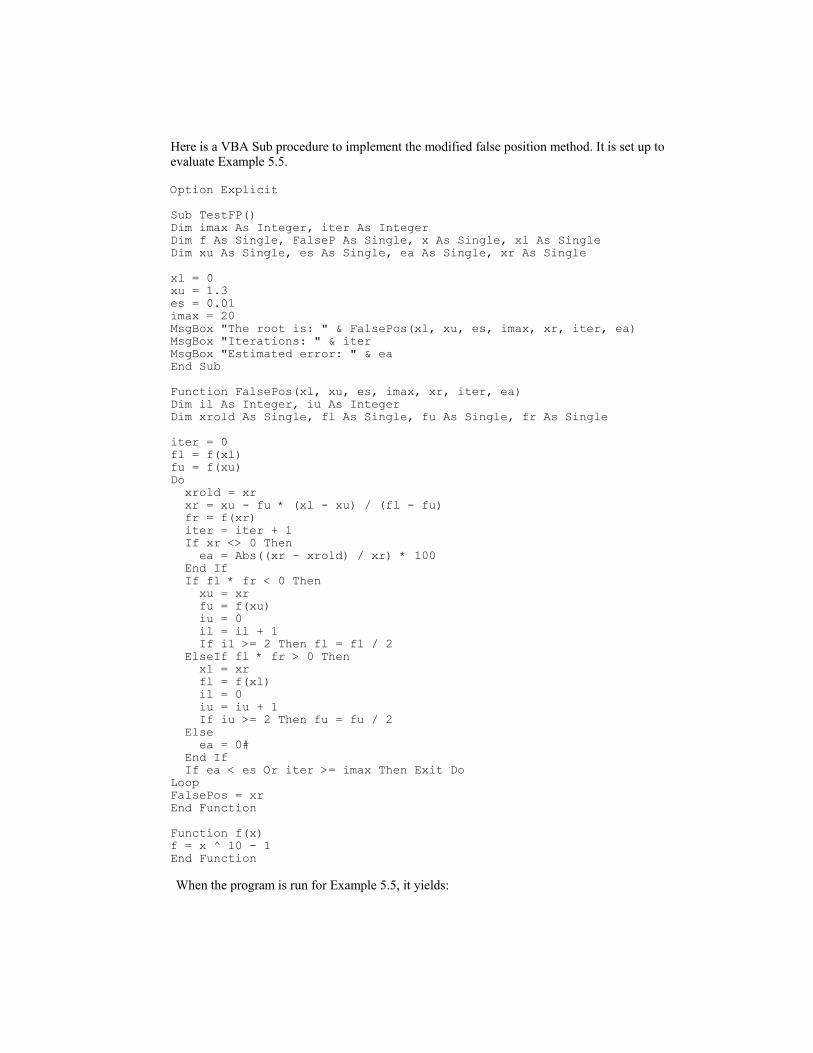
Here is a VBA Sub procedure to implement the modified false position method. It is set up toevaluate Example 5.5.
Option Explicit
Sub TestFP()Dim imax As Integer, iter As IntegerDim f As Single, FalseP As Single, x As Single, xl As SingleDim xu As Single, es As Single, ea As Single, xr As Single
xl = 0xu = 1.3es = 0.01imax = 20MsgBox "The root is: " & FalsePos(xl, xu, es, imax, xr, iter, ea)MsgBox "Iterations: " & iterMsgBox "Estimated error: " & eaEnd Sub
Function FalsePos(xl, xu, es, imax, xr, iter, ea)Dim il As Integer, iu As IntegerDim xrold As Single, fl As Single, fu As Single, fr As Single
iter = 0fl = f(xl)fu = f(xu)Do xrold = xr xr = xu - fu * (xl - xu) / (fl - fu) fr = f(xr) iter = iter + 1 If xr <> 0 Then ea = Abs((xr - xrold) / xr) * 100 End If If fl * fr < 0 Then xu = xr fu = f(xu) iu = 0 il = il + 1 If il >= 2 Then fl = fl / 2 ElseIf fl * fr > 0 Then xl = xr fl = f(xl) il = 0 iu = iu + 1 If iu >= 2 Then fu = fu / 2 Else ea = 0# End If If ea < es Or iter >= imax Then Exit DoLoopFalsePos = xrEnd Function
Function f(x)f = x ^ 10 - 1End Function
When the program is run for Example 5.5, it yields:

root = 14.7802iterations = 5
error = 3.9×10⁻⁵ %
5.17 Errata in Problem statement: Use the subprogram you developed in Prob. 5.16 to
duplicate the computation from Example 5.6.
The results are plotted as
0.001
0.01
0.1
1
10
100
1000
0 4 8 12
ea%
et,%
es,%
Interpretation: At first, the method manifests slow convergence. However, as it approachesthe root, it approaches quadratic convergence. Note also that after the first few iterations, the
approximate error estimate has the nice property that εa > εt.
5.18 Here is a VBA Sub procedure to implement the false position method with minimalfunction evaluations set up to evaluate Example 5.6.
Option ExplicitSub TestFP()Dim imax As Integer, iter As Integer, i As IntegerDim xl As Single, xu As Single, es As Single, ea As Single, xr AsSingle, fct As SingleMsgBox "The root is: " & FPMinFctEval(xl, xu, es, imax, xr, iter, ea)MsgBox "Iterations: " & iterMsgBox "Estimated error: " & eaEnd Sub
Function FPMinFctEval(xl, xu, es, imax, xr, iter, ea)Dim xrold, test, fl, fu, friter = 0xl = 0#xu = 1.3es = 0.01imax = 50fl = f(xl)fu = f(xu)xr = (xl + xu) / 2Do xrold = xr xr = xu - fu * (xl - xu) / (fl - fu) fr = f(xr)

iter = iter + 1 If (xr <> 0) Then ea = Abs((xr - xrold) / xr) * 100# End If test = fl * fr If (test < 0) Then xu = xr fu = fr ElseIf (test > 0) Then xl = xr fl = fr Else ea = 0# End If If ea < es Or iter >= imax Then Exit DoLoopFPMinFctEval = xrEnd Function
Function f(x)f = x ^ 10 - 1End Function
The program yields a root of 0.9996887 after 39 iterations. The approximate error at this
point is 9.5×10⁻³ %. These results are all displayed as message boxes. For example, the
solution check is displayed as
The number of function evaluations for this version is 2n+2. This is much smaller than thenumber of function evaluations in the standard false position method (5n).
5.19 Solve for the reactions:
R1=265 lbs. R2= 285 lbs.
Write beam equations:
0<x<33
2
55.5265)1(
02653
)667.16(
xM
xx
xM
−=
=−+
3<x<6
15041550)2(
0265))3(3
2(150)
2
3)(3(100
2 −+−=
=−−+−
−+
xxM
xxx
xM
6<x<10
1650185)3(
265)5.4(300))3(3
2(150
+−=
−−+−=
xM
xxxM
10<x<121200100)4(
0)12(100
−=
=−+
xM
xM
Combining Equations:

Because the curve crosses the axis between 6 and 10, use (3).
(3) 1650185 +−= xM
Set 10;6 == UL xx
200)(
540)( L
−=
=
UxM
xM8
2=
+= UL
r
xxx
LR xreplacesxM →= 170)(
200)(
170)( L
−=
=
UxM
xM9
2
108=
+=rx
UR xreplacesxM →−= 15)(
15)(
170)( L
−=
=
UxM
xM5.8
2
98=
+=rx
LR xreplacesxM →= 5.77)(
15)(
5.77)( L
−=
=
UxM
xM75.8
2
95.8=
+=rx
LR xreplacesxM →= 25.31)(
15)(
25.31)( L
−=
=
UxM
xM875.8
2
975.8=
+=rx
LR xreplacesxM →= 125.8)(
15)(
125.8)( L
−=
=
UxM
xM9375.8
2
9875.8=
+=rx
UR xreplacesxM →−= 4375.3)(
4375.3)(
125.8)( L
−=
=
UxM
xM90625.8
2
9375.8875.8=
+=rx
LR xreplacesxM →= 34375.2)(
4375.3)(
34375.2)( L
−=
=
UxM
xM921875.8
2
9375.890625.8=
+=rx
UR xreplacesxM →−= 546875.0)(

546875.0)(
34375.2)( L
−=
=
UxM
xM9140625.8
2
921875.890625.8=
+=rx
8984.0)( R =xM Therefore, feetx 91.8=
5.20 1650185 +−= xM
Set 10;6 == UL xx
200)(
540)( L
−=
=
UxM
xM
0102)(
9189.8)200(540
)106(20010
)()(
))((
7 ≅×−=
=−−−−
−=
−
−−=
−R
R
UL
ULUoR
xM
x
xMxM
xxxMxx
Only one iteration was necessary.
Therefore, .9189.8 feetx =


6.16Here is a VBA program to implement the Newton-Raphson algorithm and solve Example6.3.
Option Explicit
Sub NewtRaph()
Dim imax As Integer, iter As IntegerDim x0 As Single, es As Single, ea As Single
x0 = 0#es = 0.01imax = 20MsgBox "Root: " & NewtR(x0, es, imax, iter, ea)MsgBox "Iterations: " & iterMsgBox "Estimated error: " & ea
End Sub
Function df(x)df = -Exp(-x) - 1#End Function
Function f(x)f = Exp(-x) - xEnd Function
Function NewtR(x0, es, imax, iter, ea)
Dim xr As Single, xrold As Single
xr = x0iter = 0Do

xrold = xr xr = xr - f(xr) / df(xr) iter = iter + 1 If (xr <> 0) Then ea = Abs((xr - xrold) / xr) * 100 End If If ea < es Or iter >= imax Then Exit DoLoopNewtR = xrEnd Function
It’s application yields a root of 0.5671433 after 4 iterations. The approximate error at this
point is 2.1×10⁻⁵ %.
6.17Here is a VBA program to implement the secant algorithm and solve Example 6.6.
Option Explicit
Sub SecMain()Dim imax As Integer, iter As IntegerDim x0 As Single, x1 As Single, xr As SingleDim es As Single, ea As Singlex0 = 0x1 = 1es = 0.01imax = 20MsgBox "Root: " & Secant(x0, x1, xr, es, imax, iter, ea)MsgBox "Iterations: " & iterMsgBox "Estimated error: " & ea
End Sub
Function f(x)f = Exp(-x) - xEnd Function
Function Secant(x0, x1, xr, es, imax, iter, ea)xr = x1iter = 0Do xr = x1 - f(x1) * (x0 - x1) / (f(x0) - f(x1)) iter = iter + 1 If (xr <> 0) Then ea = Abs((xr - x1) / xr) * 100 End If If ea < es Or iter >= imax Then Exit Do x0 = x1 x1 = xrLoopSecant = xrEnd Function
It’s application yields a root of 0.5671433 after 4 iterations. The approximate error at this
point is 4.77×10⁻³ %.
6.18

Here is a VBA program to implement the modified secant algorithm and solve Example 6.8.
Option Explicit
Sub SecMod()Dim imax As Integer, iter As IntegerDim x As Single, es As Single, ea As Singlex = 1es = 0.01imax = 20MsgBox "Root: " & ModSecant(x, es, imax, iter, ea)MsgBox "Iterations: " & iterMsgBox "Estimated error: " & ea
End Sub
Function f(x)f = Exp(-x) - xEnd Function
Function ModSecant(x, es, imax, iter, ea)Dim xr As Single, xrold As Single, fr As SingleConst del As Single = 0.01xr = xiter = 0Do xrold = xr fr = f(xr) xr = xr - fr * del * xr / (f(xr + del * xr) - fr) iter = iter + 1 If (xr <> 0) Then ea = Abs((xr - xrold) / xr) * 100 End If If ea < es Or iter >= imax Then Exit DoLoopModSecant = xrEnd Function
It’s application yields a root of 0.5671433 after 4 iterations. The approximate error at this
point is 3.15×10⁻⁵ %.
6.19Here is a VBA program to implement the 2 equation Newton-Raphson method and solveExample 6.10.
Option Explicit
Sub NewtRaphSyst()
Dim imax As Integer, iter As IntegerDim x0 As Single, y0 As SingleDim xr As Single, yr As SingleDim es As Single, ea As Single
x0 = 1.5y0 = 3.5
es = 0.01imax = 20

Call NR2Eqs(x0, y0, xr, yr, es, imax, iter, ea)
MsgBox "x, y = " & xr & ", " & yrMsgBox "Iterations: " & iterMsgBox "Estimated error: " & ea
End SubSub NR2Eqs(x0, y0, xr, yr, es, imax, iter, ea)
Dim J As Single, eay As Single
iter = 0Do J = dudx(x0, y0) * dvdy(x0, y0) - dudy(x0, y0) * dvdx(x0, y0) xr = x0 - (u(x0, y0) * dvdy(x0, y0) - v(x0, y0) * dudy(x0, y0)) / J yr = y0 - (v(x0, y0) * dudx(x0, y0) - u(x0, y0) * dvdx(x0, y0)) / J iter = iter + 1 If (xr <> 0) Then ea = Abs((xr - x0) / xr) * 100 End If If (xr <> 0) Then eay = Abs((yr - y0) / yr) * 100 End If If eay > ea Then ea = eay If ea < es Or iter >= imax Then Exit Do x0 = xr y0 = yrLoop
End Sub
Function u(x, y)u = x ^ 2 + x * y - 10End Function
Function v(x, y)v = y + 3 * x * y ^ 2 - 57End Function
Function dudx(x, y)dudx = 2 * x + yEnd Function
Function dudy(x, y)dudy = xEnd Function
Function dvdx(x, y)dvdx = 3 * y ^ 2End Function
Function dvdy(x, y)dvdy = 1 + 6 * x * yEnd Function
It’s application yields roots of x = 2 and y = 3 after 4 iterations. The approximate error at this
point is 1.59×10⁻⁵ %.
6.20The program from Prob. 6.19 can be set up to solve Prob. 6.11, by changing the functions to

Function u(x, y)u = y + x ^ 2 - 0.5 - xEnd Function
Function v(x, y)v = x ^ 2 - 5 * x * y - yEnd Function
Function dudx(x, y)dudx = 2 * x - 1End Function
Function dudy(x, y)dudy = 1End Function
Function dvdx(x, y)dvdx = 2 * x ^ 2 - 5 * yEnd Function
Function dvdy(x, y)dvdy = -5 * xEnd Function
Using a stopping criterion of 0.01%, the program yields x = 1.233318 and y = 0.212245 after
7 iterations with an approximate error of 2.2×10⁻⁴.
The program from Prob. 6.19 can be set up to solve Prob. 6.12, by changing the functions to
Function u(x, y)u = (x - 4) ^ 2 + (y - 4) ^ 2 - 4End Function
Function v(x, y)v = x ^ 2 + y ^ 2 - 16End Function
Function dudx(x, y)dudx = 2 * (x - 4)End Function
Function dudy(x, y)dudy = 2 * (y - 4)End Function
Function dvdx(x, y)dvdx = 2 * xEnd Function
Function dvdy(x, y)dvdy = 2 * yEnd Function
Using a stopping criterion of 0.01% and initial guesses of 2 and 3.5, the program yields x =
2.0888542 and y = 3.411438 after 3 iterations with an approximate error of 9.8×10⁻⁴.

Using a stopping criterion of 0.01% and initial guesses of 3.5 and 2, the program yields x =
3.411438 and y = 2.0888542 after 3 iterations with an approximate error of 9.8×10⁻⁴.
6.21
ax =
ax =2
0)( 2 =−= axxf
xxf 2)(' =
Substitute into Newton Raphson formula (Eq. 6.6),
x
axxx
2
2 −−=
Combining terms gives
2
/
2
)(2 22 xaxaxxxx
+=
+−=
6.22SOLUTION:
( ) ( )( ) ( )[ ]( )
1.3
29sech'
9tanh
22
2
=
−=
−=
ox
xxxf
xxf
( )( )xfxf
xx ii '1 −=+
iteration xi+1
1 2.9753
2 3.2267
3 2.5774
4 7.9865
The solution diverges from its real root of x = 3. Due to the concavity of the slope, the next iterationwill always diverge. The sketch should resemble figure 6.6(a).
6.23SOLUTION:

183.1271.6852.00296.0)(
5183.12355.3284.00074.0)(
23'
234
−+−=
+−+−=
xxxxf
xxxxxf
)(
)('1
i
iii
xf
xfxx −=+
i xi+1
1 9.0767
2 -4.01014
3 -3.2726
The solution converged on another root. The partial solutions for each iteration intersected the x-axisalong its tangent path beyond a different root, resulting in convergence elsewhere.
6.24SOLUTION:
f(x) = 2)1(16 2 ++−± x
)()(
))((
1
11
ii
iiiii
xfxf
xxxfxx
−
−−=
−
−+
1st iteration
708.1)(5.0 11 −=⇒= −− ii xfx
2)(3 =⇒= ii xfx
6516.1)2708.1(
)35.0(231 =
−−
−−=+ix
2nd iteration
9948.0)(6516.1 −=⇒= ii xfx
46.1)(5.0 11−=⇒= −− ii
xfx
1142.4)9948.046.1(
)6516.15.0(9948.06516.11 =
−−−
−−−=+ix
The solution diverges because the secant created by the two x-values yields a solution outside thefunctions domain.


7.6 Errata in Fig. 7.4; 6th line from the bottom of the algorithm: the > should be changed to >=
IF (dxr < eps*xr OR iter >= maxit) EXIT
Here is a VBA program to implement the Müller algorithm and solve Example 7.2.
Option Explicit
Sub TestMull()
Dim maxit As Integer, iter As IntegerDim h As Single, xr As Single, eps As Single
h = 0.1xr = 5eps = 0.001maxit = 20
Call Muller(xr, h, eps, maxit, iter)
MsgBox "root = " & xrMsgBox "Iterations: " & iter
End Sub
Sub Muller(xr, h, eps, maxit, iter)
Dim x0 As Single, x1 As Single, x2 As SingleDim h0 As Single, h1 As Single, d0 As Single, d1 As SingleDim a As Single, b As Single, c As SingleDim den As Single, rad As Single, dxr As Single
x2 = xrx1 = xr + h * xrx0 = xr - h * xrDo iter = iter + 1 h0 = x1 - x0 h1 = x2 - x1 d0 = (f(x1) - f(x0)) / h0 d1 = (f(x2) - f(x1)) / h1 a = (d1 - d0) / (h1 + h0) b = a * h1 + d1 c = f(x2) rad = Sqr(b * b - 4 * a * c) If Abs(b + rad) > Abs(b - rad) Then den = b + rad Else den = b - rad End If dxr = -2 * c / den xr = x2 + dxr If Abs(dxr) < eps * xr Or iter >= maxit Then Exit Do x0 = x1 x1 = x2 x2 = xrLoopEnd Sub
Function f(x)f = x ^ 3 - 13 * x - 12End Function

7.7 The plot suggests a root at 1
-6
-4
-2
0
2
4
6
-1 0 1 2
Using an initial guess of 1.5 with h = 0.1 and eps = 0.001 yields the correct result of 1 in 4iterations.
7.8 Here is a VBA program to implement the Bairstow algorithm and solve Example 7.3.
Option Explicit
Sub PolyRoot()
Dim n As Integer, maxit As Integer, ier As Integer, i As IntegerDim a(10) As Single, re(10) As Single, im(10) As SingleDim r As Single, s As Single, es As Singlen = 5a(0) = 1.25: a(1) = -3.875: a(2) = 2.125: a(3) = 2.75: a(4) = -3.5: a(5) = 1maxit = 20es = 0.01r = -1s = -1Call Bairstow(a(), n, es, r, s, maxit, re(), im(), ier)For i = 1 To n If im(i) >= 0 Then MsgBox re(i) & " + " & im(i) & "i" Else MsgBox re(i) & " - " & Abs(im(i)) & "i" End IfNext i
End Sub
Sub Bairstow(a, nn, es, rr, ss, maxit, re, im, ier)
Dim iter As Integer, n As Integer, i As IntegerDim r As Single, s As Single, ea1 As Single, ea2 As SingleDim det As Single, dr As Single, ds As SingleDim r1 As Single, i1 As Single, r2 As Single, i2 As SingleDim b(10) As Single, c(10) As Single
r = rrs = ssn = nnier = 0ea1 = 1ea2 = 1Do If n < 3 Or iter >= maxit Then Exit Do iter = 0 Do iter = iter + 1 b(n) = a(n) b(n - 1) = a(n - 1) + r * b(n) c(n) = b(n) c(n - 1) = b(n - 1) + r * c(n) For i = n - 2 To 0 Step -1

b(i) = a(i) + r * b(i + 1) + s * b(i + 2) c(i) = b(i) + r * c(i + 1) + s * c(i + 2) Next i det = c(2) * c(2) - c(3) * c(1) If det <> 0 Then dr = (-b(1) * c(2) + b(0) * c(3)) / det ds = (-b(0) * c(2) + b(1) * c(1)) / det r = r + dr s = s + ds If r <> 0 Then ea1 = Abs(dr / r) * 100 If s <> 0 Then ea2 = Abs(ds / s) * 100 Else r = r + 1 s = s + 1 iter = 0 End If If ea1 <= es And ea2 <= es Or iter >= maxit Then Exit Do Loop Call Quadroot(r, s, r1, i1, r2, i2) re(n) = r1 im(n) = i1 re(n - 1) = r2 im(n - 1) = i2 n = n - 2 For i = 0 To n a(i) = b(i + 2) Next iLoopIf iter < maxit Then If n = 2 Then r = -a(1) / a(2) s = -a(0) / a(2) Call Quadroot(r, s, r1, i1, r2, i2) re(n) = r1 im(n) = i1 re(n - 1) = r2 im(n - 1) = i2 Else re(n) = -a(0) / a(1) im(n) = 0 End IfElse ier = 1End IfEnd Sub
Sub Quadroot(r, s, r1, i1, r2, i2)
Dim discdisc = r ^ 2 + 4 * sIf disc > 0 Then r1 = (r + Sqr(disc)) / 2 r2 = (r - Sqr(disc)) / 2 i1 = 0 i2 = 0Else r1 = r / 2 r2 = r1 i1 = Sqr(Abs(disc)) / 2 i2 = -i1End IfEnd Sub
7.9 See solutions to Prob. 7.5

7.10 The goal seek set up is
The result is
7.11 The goal seek set up is shown below. Notice that we have named the cells containing theparameter values with the labels in column A.
The result is 63.649 kg as shown here:

7.12 The Solver set up is shown below using initial guesses of x = y = 1. Notice that we haverearranged the two functions so that the correct values will drive them both to zero. We thendrive the sum of their squared values to zero by varying x and y. This is done because astraight sum would be zero if f1(x,y) = -f2(x,y).
The result is
7.13 A plot of the functions indicates two real roots at about (−1.5, 1.5) and (−1.5, 1.5).
-3
-2
-1
0
1
2
3
4
-3 -2 -1 0 1 2 3
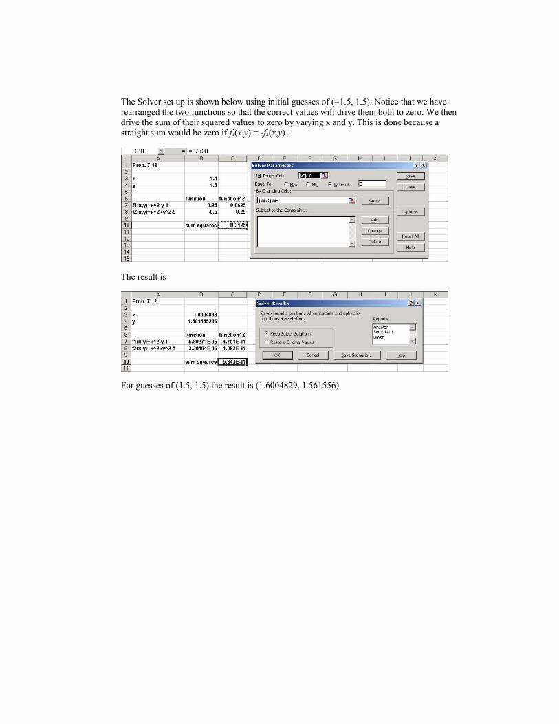
The Solver set up is shown below using initial guesses of (−1.5, 1.5). Notice that we haverearranged the two functions so that the correct values will drive them both to zero. We thendrive the sum of their squared values to zero by varying x and y. This is done because astraight sum would be zero if f1(x,y) = -f2(x,y).
The result is
For guesses of (1.5, 1.5) the result is (1.6004829, 1.561556).

>> roots (d)
with the expected result that the remaining roots of the original polynomial are found
ans = 8.0000-4.0000 1.0000
We can now multiply d by b to come up with the original polynomial,
>> conv(d,b)
ans =1 -9 -20 204 208 -384
Finally, we can determine all the roots of the original polynomial by
>> r=roots(a)
r = 8.0000 6.0000 -4.0000-2.0000 1.0000
7.15p=[0.7 -4 6.2 -2];roots(p)
ans =
3.2786
2.0000 0.4357
p=[-3.704 16.3 -21.97 9.34];roots(p)
ans =
2.2947 1.1525 0.9535
p=[1 -2 6 -2 5];roots(p)
ans =
1.0000 + 2.0000i 1.0000 - 2.0000i -0.0000 + 1.0000i -0.0000 - 1.0000i
7.16 Here is a program written in Compaq Visual Fortran 90,
PROGRAM Root
Use IMSL !This establishes the link to the IMSL libraries

Implicit None !forces declaration of all variablesInteger::nrootParameter(nroot=1)Integer::itmax=50Real::errabs=0.,errrel=1.E-5,eps=0.,eta=0.Real::f,x0(nroot) ,x(nroot)External fInteger::info(nroot)
Print *, "Enter initial guess"Read *, x0Call ZReal(f,errabs,errrel,eps,eta,nroot,itmax,x0,x,info)Print *, "root = ", xPrint *, "iterations = ", info
End
Function f(x)Implicit NoneReal::f,xf = x**3-x**2+2*x-2End
The output for Prob. 7.4a would look like
Enter initial guess.5 root = 1.000000 iterations = 7Press any key to continue
7.17ho = 0.55 – 0.53 = 0.02h1 = 0.54 – 0.55 = -0.01
δo = 58 – 19 = 1950 0.55 – 0.53
δ1 = 44 – 58 = 1400 0.54 – 0.55
a = δ 1– δ o = -55000 h1 + ho
b = a h1 + δ1 = 1950c = 44
acb 42 − = 3671.85
s 524.085.36711950
)44(254.0to =
+−
+=
Therefore, the pressure was zero at 0.524 seconds.

7.18I) Graphically:
EDU»C=[1 3.6 0 -36.4];roots(C)
ans = -3.0262+ 2.3843i -3.0262- 2.3843i
2.4524
The answer is 2.4524 considering it is the only real root.
II) Using the Roots Function:
EDU» x=-1:0.001:2.5;f=x.^3+3.6.*x.^2-36.4;plot(x,f);grid;zoom
By zooming in the plot at the desired location, we get the same answer of 2.4524.
2.4523 2.45232.4524 2.4524 2.4524 2.4524 2.45242.4524 2.4524 2.4524 2.4524
-6
-4
-2
0
2
4
x 10-4
7.19Excel Solver Solution: The 3 functions can be set up as roots problems:
02),,(
02),,(
03),,(
23
2
2221
=−−=
=−+=
=+−=
uaavuaf
vuvuaf
vuavuaf

Symbolic Manipulator Solution:
>>syms a u v>>S=solve(u^2-3*v^2-a^2,u+v-2,a^2-2*a-u)
>>double (S.a)ans = 2.9270 + 0.3050i
2.9270 – 0.3050i-0.5190-1.3350
>>double (S.u)ans = 2.6203 + 1.1753i
2.6203 – 1.1753i1.30734.4522
>>double (S.v)ans = -0.6203 + 1.1753i
-0.6203 – 1.1753i0.6297-2.4522
Therefore, we see that the two real-valued solutions for a, u, and v are (-0.5190,1.3073,0.6927) and (-1.3350,4.4522,-2.4522).
7.20 The roots of the numerator are: s = -2, s = -3, and s = -4.The roots of the denominator are: s = -1, s = -3, s = -5, and s = -6.
)6)(5)(3)(1(
)4)(3)(2()(
+++++++
=ssss
ssssG


9.14Here is a VBA program to implement matrix multiplication and solve Prob. 9.3 for the case
of [X]×[Y].
Option Explicit
Sub Mult()
Dim i As Integer, j As IntegerDim l As Integer, m As Integer, n As IntegerDim x(10, 10) As Single, y(10, 10) As SingleDim w(10, 10) As Single
l = 2m = 2n = 3x(1, 1) = 1: x(1, 2) = 6x(2, 1) = 3: x(2, 2) = 10x(3, 1) = 7: x(3, 2) = 4y(1, 1) = 6: y(2, 1) = 0y(2, 1) = 1: y(2, 2) = 4Call Mmult(x(), y(), w(), m, n, l)
For i = 1 To n For j = 1 To l MsgBox w(i, j)
Next jNext i
End Sub
Sub Mmult(y, z, x, n, m, p)
Dim i As Integer, j As Integer, k As IntegerDim sum As Single
For i = 1 To m For j = 1 To p sum = 0 For k = 1 To n sum = sum + y(i, k) * z(k, j) Next k x(i, j) = sum Next jNext i
End Sub
9.15Here is a VBA program to implement the matrix transpose and solve Prob. 9.3 for the case of[X]T.
Option Explicit
Sub Mult()
Dim i As Integer, j As IntegerDim m As Integer, n As IntegerDim x(10, 10) As Single, y(10, 10) As Single
n = 3m = 2x(1, 1) = 1: x(1, 2) = 6x(2, 1) = 3: x(2, 2) = 10

x(3, 1) = 7: x(3, 2) = 4Call MTrans(x(), y(), n, m)For i = 1 To m For j = 1 To n MsgBox y(i, j) Next jNext i
End Sub
Sub MTrans(a, b, n, m)
Dim i As Integer, j As Integer
For i = 1 To m For j = 1 To n b(i, j) = a(j, i) Next jNext i
End Sub
9.16Here is a VBA program to implement the Gauss elimination algorithm and solve the test casein Prob. 9.16.
Option Explicit
Sub GaussElim()
Dim n As Integer, er As Integer, i As IntegerDim a(10, 10) As Single, b(10) As Single, x(10) As Single
Range("a1").Selectn = 3a(1, 1) = 1: a(1, 2) = 1: a(1, 3) = -1a(2, 1) = 6: a(2, 2) = 2: a(2, 3) = 2a(3, 1) = -3: a(3, 2) = 4: a(3, 3) = 1b(1) = 1: b(2) = 10: b(3) = 2
Call Gauss(a(), b(), n, x(), er)If er = 0 Then For i = 1 To n MsgBox "x(" & i & ") = " & x(i) Next iElse MsgBox "ill-conditioned system"End If
End Sub
Sub Gauss(a, b, n, x, er) Dim i As Integer, j As IntegerDim s(10) As SingleConst tol As Single = 0.000001er = 0For i = 1 To n s(i) = Abs(a(i, 1)) For j = 2 To n If Abs(a(i, j)) > s(i) Then s(i) = Abs(a(i, j)) Next jNext iCall Eliminate(a, s(), n, b, tol, er)If er <> -1 Then

Call Substitute(a, n, b, x)End IfEnd Sub
Sub Pivot(a, b, s, n, k)Dim p As Integer, ii As Integer, jj As IntegerDim factor As Single, big As Single, dummy As Singlep = kbig = Abs(a(k, k) / s(k))For ii = k + 1 To n dummy = Abs(a(ii, k) / s(ii)) If dummy > big Then big = dummy p = ii End IfNext iiIf p <> k Then For jj = k To n dummy = a(p, jj) a(p, jj) = a(k, jj) a(k, jj) = dummy Next jj dummy = b(p) b(p) = b(k) b(k) = dummy dummy = s(p) s(p) = s(k) s(k) = dummyEnd IfEnd Sub
Sub Substitute(a, n, b, x)Dim i As Integer, j As IntegerDim sum As Singlex(n) = b(n) / a(n, n)For i = n - 1 To 1 Step -1 sum = 0 For j = i + 1 To n sum = sum + a(i, j) * x(j) Next j x(i) = (b(i) - sum) / a(i, i)Next iEnd Sub
Sub Eliminate(a, s, n, b, tol, er) Dim i As Integer, j As Integer, k As IntegerDim factor As SingleFor k = 1 To n - 1 Call Pivot(a, b, s, n, k) If Abs(a(k, k) / s(k)) < tol Then er = -1 Exit For End If For i = k + 1 To n factor = a(i, k) / a(k, k) For j = k + 1 To n a(i, j) = a(i, j) - factor * a(k, j) Next j b(i) = b(i) - factor * b(k) Next iNext kIf Abs(a(k, k) / s(k)) < tol Then er = -1End Sub
It’s application yields a solution of (1, 1, 1).

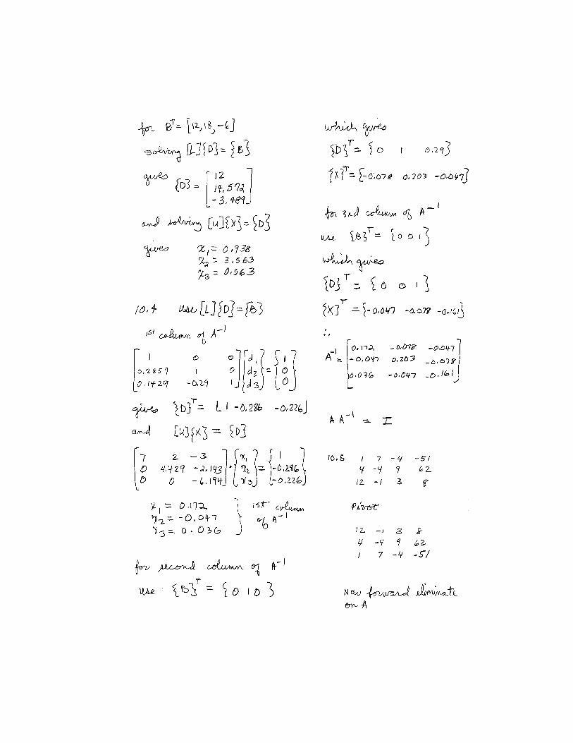


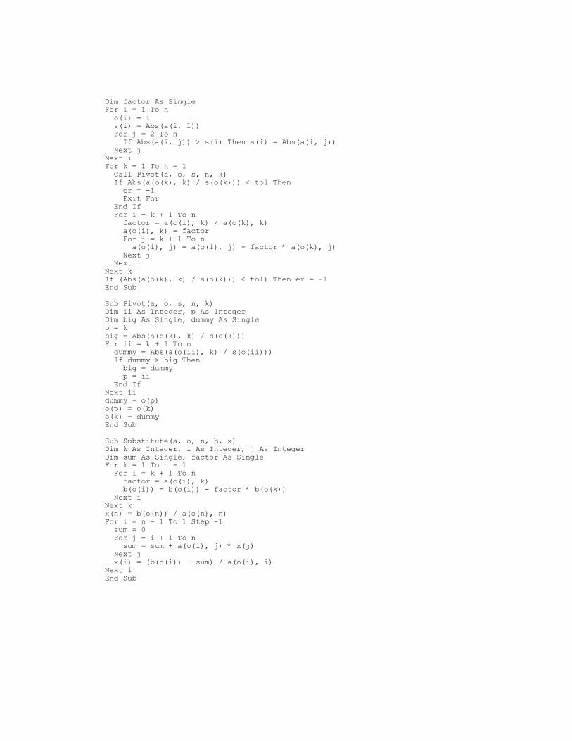
10.14
Option Explicit
Sub LUDTest()Dim n As Integer, er As Integer, i As Integer, j As IntegerDim a(3, 3) As Single, b(3) As Single, x(3) As SingleDim tol As Single
n = 3a(1, 1) = 3: a(1, 2) = -0.1: a(1, 3) = -0.2a(2, 1) = 0.1: a(2, 2) = 7: a(2, 3) = -0.3a(3, 1) = 0.3: a(3, 2) = -0.2: a(3, 3) = 10b(1) = 7.85: b(2) = -19.3: b(3) = 71.4tol = 0.000001
Call LUD(a(), b(), n, x(), tol, er)
'output results to worksheetSheets("Sheet1").SelectRange("a3").SelectFor i = 1 To n ActiveCell.Value = x(i) ActiveCell.Offset(1, 0).Select

Next iRange("a3").Select End Sub
Sub LUD(a, b, n, x, tol, er)Dim i As Integer, j As IntegerDim o(3) As Single, s(3) As SingleCall Decompose(a, n, tol, o(), s(), er)If er = 0 Then Call Substitute(a, o(), n, b, x)Else MsgBox "ill-conditioned system" EndEnd IfEnd Sub
Sub Decompose(a, n, tol, o, s, er)Dim i As Integer, j As Integer, k As IntegerDim factor As SingleFor i = 1 To n o(i) = i s(i) = Abs(a(i, 1)) For j = 2 To n If Abs(a(i, j)) > s(i) Then s(i) = Abs(a(i, j)) Next jNext iFor k = 1 To n - 1 Call Pivot(a, o, s, n, k) If Abs(a(o(k), k) / s(o(k))) < tol Then er = -1 Exit For End If
For i = k + 1 To n factor = a(o(i), k) / a(o(k), k) a(o(i), k) = factor For j = k + 1 To n a(o(i), j) = a(o(i), j) - factor * a(o(k), j) Next j Next iNext kIf (Abs(a(o(k), k) / s(o(k))) < tol) Then er = -1End Sub
Sub Pivot(a, o, s, n, k)Dim ii As Integer, p As IntegerDim big As Single, dummy As Singlep = kbig = Abs(a(o(k), k) / s(o(k)))For ii = k + 1 To n dummy = Abs(a(o(ii), k) / s(o(ii))) If dummy > big Then big = dummy p = ii End IfNext iidummy = o(p)o(p) = o(k)o(k) = dummyEnd Sub
Sub Substitute(a, o, n, b, x)Dim k As Integer, i As Integer, j As IntegerDim sum As Single, factor As SingleFor k = 1 To n - 1 For i = k + 1 To n factor = a(o(i), k)

b(o(i)) = b(o(i)) - factor * b(o(k)) Next iNext kx(n) = b(o(n)) / a(o(n), n)For i = n - 1 To 1 Step -1 sum = 0 For j = i + 1 To n sum = sum + a(o(i), j) * x(j) Next j x(i) = (b(o(i)) - sum) / a(o(i), i)Next iEnd Sub
10.15
Option Explicit
Sub LUGaussTest()Dim n As Integer, er As Integer, i As Integer, j As IntegerDim a(3, 3) As Single, b(3) As Single, x(3) As SingleDim tol As Single, ai(3, 3) As Singlen = 3a(1, 1) = 3: a(1, 2) = -0.1: a(1, 3) = -0.2a(2, 1) = 0.1: a(2, 2) = 7: a(2, 3) = -0.3a(3, 1) = 0.3: a(3, 2) = -0.2: a(3, 3) = 10tol = 0.000001Call LUDminv(a(), b(), n, x(), tol, er, ai())If er = 0 Then Range("a1").Select For i = 1 To n For j = 1 To n ActiveCell.Value = ai(i, j) ActiveCell.Offset(0, 1).Select Next j ActiveCell.Offset(1, -n).Select Next i Range("a1").SelectElse MsgBox "ill-conditioned system"End IfEnd Sub
Sub LUDminv(a, b, n, x, tol, er, ai)Dim i As Integer, j As IntegerDim o(3) As Single, s(3) As SingleCall Decompose(a, n, tol, o(), s(), er)If er = 0 Then For i = 1 To n For j = 1 To n If i = j Then b(j) = 1 Else b(j) = 0 End If Next j Call Substitute(a, o, n, b, x) For j = 1 To n ai(j, i) = x(j) Next j Next iEnd IfEnd Sub
Sub Decompose(a, n, tol, o, s, er)Dim i As Integer, j As Integer, k As Integer
Dim factor As SingleFor i = 1 To n o(i) = i s(i) = Abs(a(i, 1)) For j = 2 To n If Abs(a(i, j)) > s(i) Then s(i) = Abs(a(i, j)) Next jNext iFor k = 1 To n - 1 Call Pivot(a, o, s, n, k) If Abs(a(o(k), k) / s(o(k))) < tol Then er = -1 Exit For End If For i = k + 1 To n factor = a(o(i), k) / a(o(k), k) a(o(i), k) = factor For j = k + 1 To n a(o(i), j) = a(o(i), j) - factor * a(o(k), j) Next j Next iNext kIf (Abs(a(o(k), k) / s(o(k))) < tol) Then er = -1End Sub
Sub Pivot(a, o, s, n, k)Dim ii As Integer, p As IntegerDim big As Single, dummy As Singlep = kbig = Abs(a(o(k), k) / s(o(k)))For ii = k + 1 To n dummy = Abs(a(o(ii), k) / s(o(ii))) If dummy > big Then big = dummy p = ii End IfNext iidummy = o(p)o(p) = o(k)o(k) = dummyEnd Sub
Sub Substitute(a, o, n, b, x)Dim k As Integer, i As Integer, j As IntegerDim sum As Single, factor As SingleFor k = 1 To n - 1 For i = k + 1 To n factor = a(o(i), k) b(o(i)) = b(o(i)) - factor * b(o(k)) Next iNext kx(n) = b(o(n)) / a(o(n), n)For i = n - 1 To 1 Step -1 sum = 0 For j = i + 1 To n sum = sum + a(o(i), j) * x(j) Next j x(i) = (b(o(i)) - sum) / a(o(i), i)Next iEnd Sub

10.17
( )31032
)2(6320
)1(3240
=+⇒=⋅
−=−⇒=⋅
=+−⇒=⋅
cbCB
caCA
baBA
Solve the three equations using Matlab:
>> A=[-4 2 0; 2 0 –3; 0 3 1]b=[3; -6; 10]x=inv(A)*b
x = 0.525 2.550 2.350
Therefore, a = 0.525, b = 2.550, and c = 2.350.
10.18
kbajcaicbc
k
ba
ji
BA
)2()24()4(
412
)( +++−−−−=
−−
=×
kbajcaicbc
k
ba
ji
CA
)3()2()32(
231
)( ++−−−==×
kbajcaicbCABA
)4()2()42()()( +++−−−−=×+×

Therefore,
kcjbiarbajcaicb
)14()23()65()4()2()42( +−+−++=++−−+−−
We get the following set of equations ⇒64256542 =−−−⇒+=−− cbaacb (1)
232232 −=−−⇒−=− cbabca (2)
144144 =−+⇒+−=+ cbacba (3)
In Matlab:
A=[-5 -5 -4 ; 2 -3 -1 ; 4 1 -4]B=[ 6 ; -2 ; 1] ; x = inv (A) * b
Answer ⇒ x = -3.6522 -3.3478
4.7391
a = -3.6522, b = -3.3478, c = 4.7391
10.19
(I) 11)0(1)0( =⇒=+⇒= bbaf
121)2(1)2( =+⇒=+⇒= dcdcf
(II) If f is continuous, then at x = 1
0)1()1( =−−+⇒+=+⇒+=+ dcbadcbadcxbax
(III) 4=+ ba
=
−−
4
0
1
1
0011
1111
2200
0010
d
c
b
a
Solve using Matlab ⇒
10.20 MATLAB provides a handy way to solve this problem.
a = 3
b = 1
c = -3
d = 7

(a)>> a=hilb(3)
a = 1.0000 0.5000 0.3333 0.5000 0.3333 0.2500 0.3333 0.2500 0.2000
>> b=[1 1 1]'
b = 1 1 1
>> c=a*b
c = 1.8333 1.0833 0.7833
>> format long e
>> x=a\b
>> x =
9.999999999999991e-001 1.000000000000007e+000 9.999999999999926e-001
(b)>> a=hilb(7);>> b=[1 1 1 1 1 1 1]';>> c=a*b;>> x=a\bx =
9.999999999914417e-001 1.000000000344746e+000 9.999999966568566e-001 1.000000013060454e+000 9.999999759661609e-001 1.000000020830062e+000 9.999999931438059e-001
(c)>> a=hilb(10);>> b=[1 1 1 1 1 1 1 1 1 1]';>> c=a*b;>> x=a\b
x = 9.999999987546324e-001 1.000000107466305e+000 9.999977129981819e-001 1.000020777695979e+000 9.999009454847158e-001 1.000272183037448e+000 9.995535966572223e-001 1.000431255894815e+000 9.997736605804316e-001 1.000049762292970e+000


Matlab solution to Prob. 11.11 (ii):
a=[1 4 9 16;4 9 16 25;9 16 25 36;16 25 36 49]
a =
1 4 9 16 4 9 16 25 9 16 25 36 16 25 36 49
b=[30 54 86 126]
b =
30 54 86 126
b=b'
b =
30 54 86 126
x=a\bWarning: Matrix is close to singular or badly scaled. Results may be inaccurate. RCOND = 2.092682e-018.
x =
1.1053 0.6842 1.3158 0.8947
x=inv(a)*bWarning: Matrix is close to singular or badly scaled. Results may be inaccurate. RCOND = 2.092682e-018.
x =
0 0 0 0
cond(a)
ans =
4.0221e+017

11.12
Program LinsimpUse IMSLImplicit NoneInteger::ipath,lda,n,ldfacParameter(ipath=1,lda=3,ldfac=3,n=3)Integer::ipvt(n),i,jReal::A(lda,lda),Rcond,Res(n)Real::Rj(n),B(n),X(n)Data A/1.0,0.5,0.3333333,0.5,0.3333333,0.25,0.3333333,0.25,0.2/Data B/1.833333,1.083333,0.783333/
Call linsol(n,A,B,X,Rcond)Print *, 'Condition number = ', 1.0E0/RcondPrint *Print *, 'Solution:'Do I = 1,n Print *, X(i)End DoEnd Program
Subroutine linsol(n,A,B,X,Rcond)Implicit noneInteger::n, ipvt(3)Real::A(n,n), fac(n,n), Rcond, res(n)Real::B(n), X(n)Call lfcrg(n,A,3,fac,3,ipvt,Rcond)Call lfirg(n,A,3,fac,3,ipvt,B,1,X,res)End
11.13
Option Explicit
Sub TestChol()
Dim i As Integer, j As IntegerDim n As IntegerDim a(10, 10) As Single
n = 3a(1, 1) = 6: a(1, 2) = 15: a(1, 3) = 55a(2, 1) = 15: a(2, 2) = 55: a(2, 3) = 225a(3, 1) = 55: a(3, 2) = 225: a(3, 3) = 979
Call Cholesky(a(), n)
'output results to worksheetSheets("Sheet1").SelectRange("a3").SelectFor i = 1 To n For j = 1 To n ActiveCell.Value = a(i, j) ActiveCell.Offset(0, 1).Select Next j ActiveCell.Offset(1, -n).SelectNext iRange("a3").Select
End SubSub Cholesky(a, n)
Dim i As Integer, j As Integer, k As IntegerDim sum As Single

For k = 1 To n For i = 1 To k - 1 sum = 0 For j = 1 To i - 1 sum = sum + a(i, j) * a(k, j) Next j a(k, i) = (a(k, i) - sum) / a(i, i) Next i sum = 0 For j = 1 To k - 1 sum = sum + a(k, j) ^ 2 Next j a(k, k) = Sqr(a(k, k) - sum)Next k
End Sub
11.14
Option Explicit
Sub Gausseid()Dim n As Integer, imax As Integer, i As IntegerDim a(3, 3) As Single, b(3) As Single, x(3) As SingleDim es As Single, lambda As Singlen = 3a(1, 1) = 3: a(1, 2) = -0.1: a(1, 3) = -0.2a(2, 1) = 0.1: a(2, 2) = 7: a(2, 3) = -0.3a(3, 1) = 0.3: a(3, 2) = -0.2: a(3, 3) = 10b(1) = 7.85: b(2) = -19.3: b(3) = 71.4es = 0.1imax = 20lambda = 1#Call Gseid(a(), b(), n, x(), imax, es, lambda)For i = 1 To n MsgBox x(i)Next iEnd Sub
Sub Gseid(a, b, n, x, imax, es, lambda)Dim i As Integer, j As Integer, iter As Integer, sentinel As IntegerDim dummy As Single, sum As Single, ea As Single, old As SingleFor i = 1 To n dummy = a(i, i) For j = 1 To n a(i, j) = a(i, j) / dummy Next j b(i) = b(i) / dummyNext iFor i = 1 To n sum = b(i) For j = 1 To n If i <> j Then sum = sum - a(i, j) * x(j) Next j x(i) = sumNext iiter = 1Do sentinel = 1 For i = 1 To n old = x(i) sum = b(i) For j = 1 To n If i <> j Then sum = sum - a(i, j) * x(j) Next j

x(i) = lambda * sum + (1# - lambda) * old If sentinel = 1 And x(i) <> 0 Then ea = Abs((x(i) - old) / x(i)) * 100 If ea > es Then sentinel = 0 End If Next i iter = iter + 1 If sentinel = 1 Or iter >= imax Then Exit DoLoopEnd Sub
11.15 As shown, there are 4 roots, one in each quadrant.
-8
-4
0
4
8
-4 -2 0 2
f
g
(−2, −4)
(−0.618,3.236)
(1, 2)
(1.618, −1.236)
It might be expected that if an initial guess was within a quadrant, the result wouls be theroot in the quadrant. However a sample of initial guesses spanning the range yield thefollowing roots:
6 (-2, -4) (-0.618,3.236) (-0.618,3.236) (1,2) (-0.618,3.236)
3 (-0.618,3.236) (-0.618,3.236) (-0.618,3.236) (1,2) (-0.618,3.236)
0 (1,2) (1.618, -1.236) (1.618, -1.236) (1.618, -1.236) (1.618, -1.236)
-3 (-2, -4) (-2, -4) (1.618, -1.236) (1.618, -1.236) (1.618, -1.236)
-6 (-2, -4) (-2, -4) (-2, -4) (1.618, -1.236) (-2, -4)
-6 -3 0 3 6
We have highlighted the guesses that converge to the roots in their quadrants. Althoughsome follow the pattern, others jump to roots that are far away. For example, the guess of(-6, 0) jumps to the root in the first quadrant.
This underscores the notion that root location techniques are highly sensitive to initialguesses and that open methods like the Solver can locate roots that are not in the vicinity ofthe initial guesses.
11.16
x = transistorsy = resistorsz = computer chips
System equations: 810233 =++ zyx
4102 =++ zyx
49022 =++ zyx

Let A =
212
121
233
and B =
490
410
810
Plug into Excel and use two functions- minverse mmult
Apply Ax = B x = A-1 * B
Answer: x = 100, y = 110, z = 90
11.17 As ordered, none of the sets will converge. However, if Set 1 and 3 are reordered so thatthey are diagonally dominant, they will converge on the solution of (1, 1, 1).
Set 1: 8x + 3y + z = 12 2x + 4y – z = 5
−6x +7z = 1
Set 3: 3x + y − z = 3 x + 4y – z = 4 x + y +5z =7
At face value, because it is not diagonally dominant, Set 2 would seem to be divergent.However, since it is close to being diagonally dominant, a solution can be obtained by thefollowing ordering:
Set 3: −2x + 2y − 3z = −3 2y – z = 1
−x + 4y + 5z = 8
11.18
Option Explicit
Sub TriDiag()Dim i As Integer, n As IntegerDim e(10) As Single, f(10) As Single, g(10) As SingleDim r(10) As Single, x(10) As Singlen = 4e(2) = -1.2: e(3) = -1.2: e(4) = -1.2f(1) = 2.04: f(2) = 2.04: f(3) = 2.04: f(4) = 2.04g(1) = -1: g(2) = -1: g(3) = -1r(1) = 40.8: r(2) = 0.8: r(3) = 0.8: r(4) = 200.8Call Thomas(e(), f(), g(), r(), n, x())For i = 1 To n MsgBox x(i)Next iEnd Sub
Sub Thomas(e, f, g, r, n, x)Call Decomp(e, f, g, n)Call Substitute(e, f, g, r, n, x)End Sub

Sub Decomp(e, f, g, n)Dim k As IntegerFor k = 2 To n e(k) = e(k) / f(k - 1) f(k) = f(k) - e(k) * g(k - 1)Next kEnd Sub
Sub Substitute(e, f, g, r, n, x)Dim k As IntegerFor k = 2 To n r(k) = r(k) - e(k) * r(k - 1)Next kx(n) = r(n) / f(n)For k = n - 1 To 1 Step -1 x(k) = (r(k) - g(k) * x(k + 1)) / f(k)Next kEnd Sub
11.19 The multiplies and divides are noted below
Sub Decomp(e, f, g, n)Dim k As IntegerFor k = 2 To n
e(k) = e(k) / f(k - 1) '(n – 1)
f(k) = f(k) - e(k) * g(k - 1) '(n – 1)
Next kEnd Sub
Sub Substitute(e, f, g, r, n, x)Dim k As IntegerFor k = 2 To n
r(k) = r(k) - e(k) * r(k - 1) '(n – 1)
Next k
x(n) = r(n) / f(n) ' 1
For k = n - 1 To 1 Step -1
x(k) = (r(k) - g(k) * x(k + 1)) / f(k) '2(n – 1)
Next kEnd Sub
Sum = 5(n-1) + 1
They can be summed to yield 5(n – 1) + 1 as opposed to n3/3 for naive Gauss elimination.Therefore, a tridiagonal solver is well worth using.
1
10
100
1000
10000
100000
1000000
1 10 100
Tridiagonal
Naive Gauss
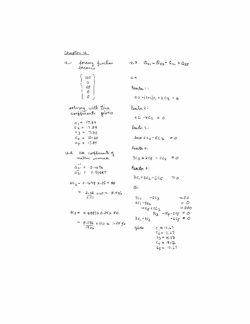

12.9
)2(0383.03665.0
080sin37sin5.21sin:0
)1(09723.093042.0
080cos37cos5.21cos:0
=−
=−+=+↑
=−
=−−=+→
∑
∑
MP
MMPF
MP
MMPF
y
x
Use any method to solve equations (1) and (2):
=
−
+−=
0
0
)80sin37(sin5.21sin
)80cos37(cos5.21cos
B
A
Apply Ax = B where x =
M
P
Use Matlab or calculator for results
P = 314 lbM = 300 lb

12.10 Mass balances can be written for each reactor as
1,111,inin,in 0 AAA cVkcQcQ −−=
1,111,in 0 AB cVkcQ +=
2,222,32in3,321,in )( 0 AAAA cVkcQQcQcQ −+−+=
2,222,32in3,321,in )( 0 ABBB cVkcQQcQcQ ++−+=
3,333,43in4,432,32in )()( 0 AAAA cVkcQQcQcQQ −+−++=
3,333,43in4,432,32in )()( 0 ABBB cVkcQQcQcQQ ++−++=
4,444,43in3,43in )()( 0 AAA cVkcQQcQQ −+−+=
4,444,43in3,43in )()( 0 ABB cVkcQQcQQ ++−+=
Collecting terms, the system can be expresses in matrix form as
[A]{C} = {B}
where
[A] =
−−−
−−−−−
−−−−−
−
135.2130000005.15013000030185015000
03068015000050155.7100000505.220100000001025.1000000025.11
[B]T = [10 0 0 0 0 0 0 0 0 0] [C]T = [cA,1 cB,1 cA,2 cB,2 cA,3 cB,3 cA,4 cB,4]
The system can be solved for [C]T = [0.889 0.111 0.416 0.584 0.095 0.905 0.0800.920].
A
B
0
0.2
0.4
0.6
0.8
1
0 1 2 3 4
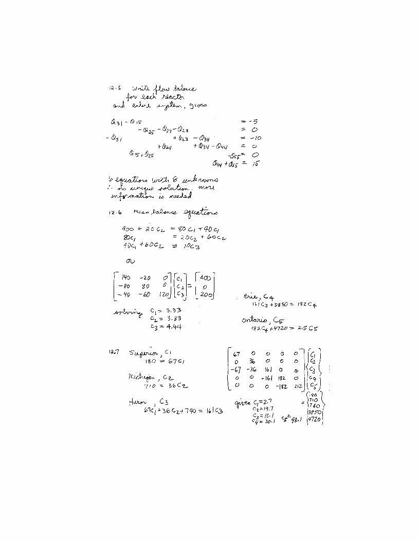
12.11 Assuming a unit flow for Q1, the simultaneous equations can be written in matrix formas

=
−−−−
−−
−
001000
111000001110000011310000012100000121
7
6
5
4
3
2
Q
Q
Q
Q
Q
Q
These equations can be solved to give [Q]T = [0.7321 0.2679 0.1964 0.0714 0.05360.0178].


12.20 Find the unit vectors:
kjikji
B
kjikji
A
ˆ873.0ˆ218.0ˆ436.0421
ˆ4ˆ1ˆ2
ˆ873.0ˆ436.0ˆ218.0421
ˆ4ˆ2ˆ1
222
222
−+=
++
−+
−−=
++
−−
Sum moments about the origin:
0)4(218.0)4(436.0
0)4(218.0)4(436.0)2(50
=−=
=−−=
∑
∑
BAM
ABM
oy
ox
Solve for A & B using equations 9.10 and 9.11:
In the form2222221
1212111
bxaxa
bxaxa
=+
=+

0872.0744.1
100744.1872.0
=−+
−=−+−
BA
BA
Plug into equations 9.10 and 9.11:
Naaaa
babax
Naaaa
babax
87.4580192.3
4.174
94.2280192.3
2.87
21122211
1212112
21122211
2121221
==−
−=
==−
−=
12.21
kjikji
T ˆ549.0ˆ824.0ˆ1374.0461
ˆ4ˆ6ˆ1
222−+=
++
−+
0)1(549.0)1(5 =−+−=∑ TM y
kNT 107.9=
kNTkNTkNT zyx 5 , 50.7 , 251.1 −===∴
0)3()3(5)4(5.7)3(5 =+−+−+−=∑ zx BM kNBz 20=
0)3()3(251.1)3(5.7 =++=∑ xz BM
kNBx 751.3−=
02055 =++−+−=∑ zz AF
kNAz 10−=
0251.1751.3 =+−+=∑ xx AF kNAx 5.2=
050.7 =+=∑ yy AF kNAy 5.7−=
12.22 This problem was solved using Matlab.
A = [1 0 0 0 0 0 0 0 1 0 0 0 1 0 0 0 0 1 0 0 0 1 0 3/5 0 0 0 0 0 0 -1 0 0 -4/5 0 0 0 0 0 0 0 -1 0 0 0 0 3/5 0 0 0 0 0 0 0 -1 0 -4/5 0 0 0 0 0 -1 -3/5 0 1 0 0 0 0 0 0 0 4/5 1 0 0 0 0 0 0 0 0 0 0 -1 -3/5 0 0 0 0 0 0 0 0 0 4/5 0 0 1];
b = [0 0 –54 0 0 24 0 0 0 0];
x=inv(A)*b
x =

24.0000 -36.0000 54.0000 -30.0000 24.0000 36.0000 -60.0000 -54.0000 -24.0000 48.0000
Therefore, in kN
AB = 24 BC = −36 AD = 54 BD = −30 CD = 24
DE = 36 CE = −60 Ax = −54 Ay = −24 Ey = 48


12.27 This problem can be solved directly on a calculator capable of doing matrix operationsor on Matlab.
a=[60 -40 0 -40 150 -100 0 -100 130];b=[200 0 230];
x=inv(a)*b
x =
7.7901 6.6851 6.9116
Therefore,
I1 = 7.79 AI2 = 6.69 AI3 = 6.91 A
12.28 This problem can be solved directly on a calculator capable of doing matrix operationsor on Matlab.
a=[17 -8 -3

-2 6 -3 -1 -4 13];b=[480 0 0];
x=inv(a)*b
x =
37.3585 16.4151 7.9245
Therefore,
V1 = 37.4 VV2 = 16.42 VV3 = 7.92 V
12.29 This problem can be solved directly on a calculator capable of doing matrix operationsor on Matlab.
a=[6 0 -4 1 0 8 -8 -1 -4 -8 18 0 -1 1 0 0];
b=[0 -20 0 10];
x=inv(a)*b
x =
-7.7778 2.2222 -0.7407 43.7037
Therefore,
I1 = -7.77 AI2 = 2.22 AI3 = -.741 AVs = 43.7 V
12.30 This problem can be solved directly on a calculator capable of doing matrix operationsor on Matlab.
a=[55 0 -25 0 37 -4 -25 -4 29];b=[-200 -250 100];
x=inv(a)*b

x =
-4.1103 -6.8695 -1.0426
Therefore,
I1 = -4.11 AI3 = -6.87 A
I4 = -1.043 A


12.37
%massspring34.m
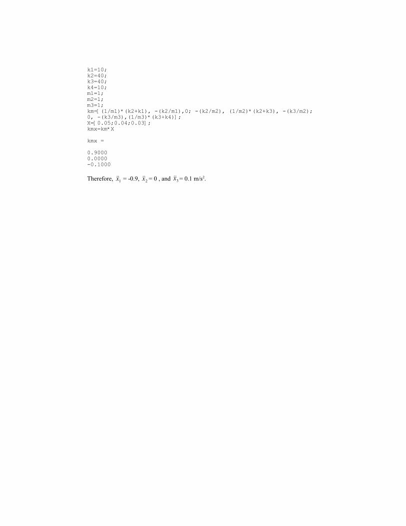
k1=10;k2=40;k3=40;k4=10;m1=1;m2=1;m3=1;km=[(1/m1)*(k2+k1), -(k2/m1),0; -(k2/m2), (1/m2)*(k2+k3), -(k3/m2);0, -(k3/m3),(1/m3)*(k3+k4)];X=[0.05;0.04;0.03];kmx=km*X
kmx =
0.90000.0000-0.1000
Therefore, 1x = -0.9, 2x = 0 , and 3x = 0.1 m/s2.

CHAPTER 16
16.4 (a) The total LP formulation is given by
Maximize C X Y Z= + +015 0 025 0 05. . . {Maximize profit}
subject to
X Y Z+ + ≥ 6 {Material constraint}
X Y+ < 3 {Time constraint}
X Y− ≥ 0 {Storage constraint}
Z Y− ≥0 5 0. {Positivity constraints}
(b) The simplex tableau for the problem can be set up and solved as
(c) An Excel spreadsheet can be set up to solve the problem as
The Solver can be called and set up as
The resulting solution is
In addition, a sensitivity report can be generated as
(d) The high shadow price for storage from the sensitivity analysis from (c) suggests thatincreasing storage will result in the best increase in profit.
16.5 An LP formulation for this problem can be set up as
Maximize C X Y Z= + +015 0 025 0 05. . . {Maximize profit}
subject to
X Y Z+ + ≥ 6 {X material constraint}
X Y+ < 3 {Y material constraint}
X Y− ≥ 0 {Waste constraint}
Z Y− ≥0 5 0. {Positivity constraints}
(b) An Excel spreadsheet can be set up to solve the problem as
The Solver can be called and set up as
The resulting solution is
This is an interesting result which might seem counterintuitive at first. Notice that wecreate some of the unprofitable z2 while producing none of the profitable z3. This occurredbecause we used up all of Y in producing the highly profitable z1. Thus, there was none leftto produce z3.
16.6 Substitute xB = 1 – xT into the pressure equation,
PPxPxTB satTsatT =+− )1(
and solve for xT,
BT
B
satsat
sat
TPP
PPx
−
−= (1)
where the partial pressures are computed as
+
−
= 221
1211905.6
10 TsatBP

+
−
= 219
1344953.6
10 TsatBP
The solution then consists of maximizing Eq. 1 by varying T subject to the constraint that 0
≤ xT ≤ 1. The Excel solver can be used to obtain the solution of T = 111.04.
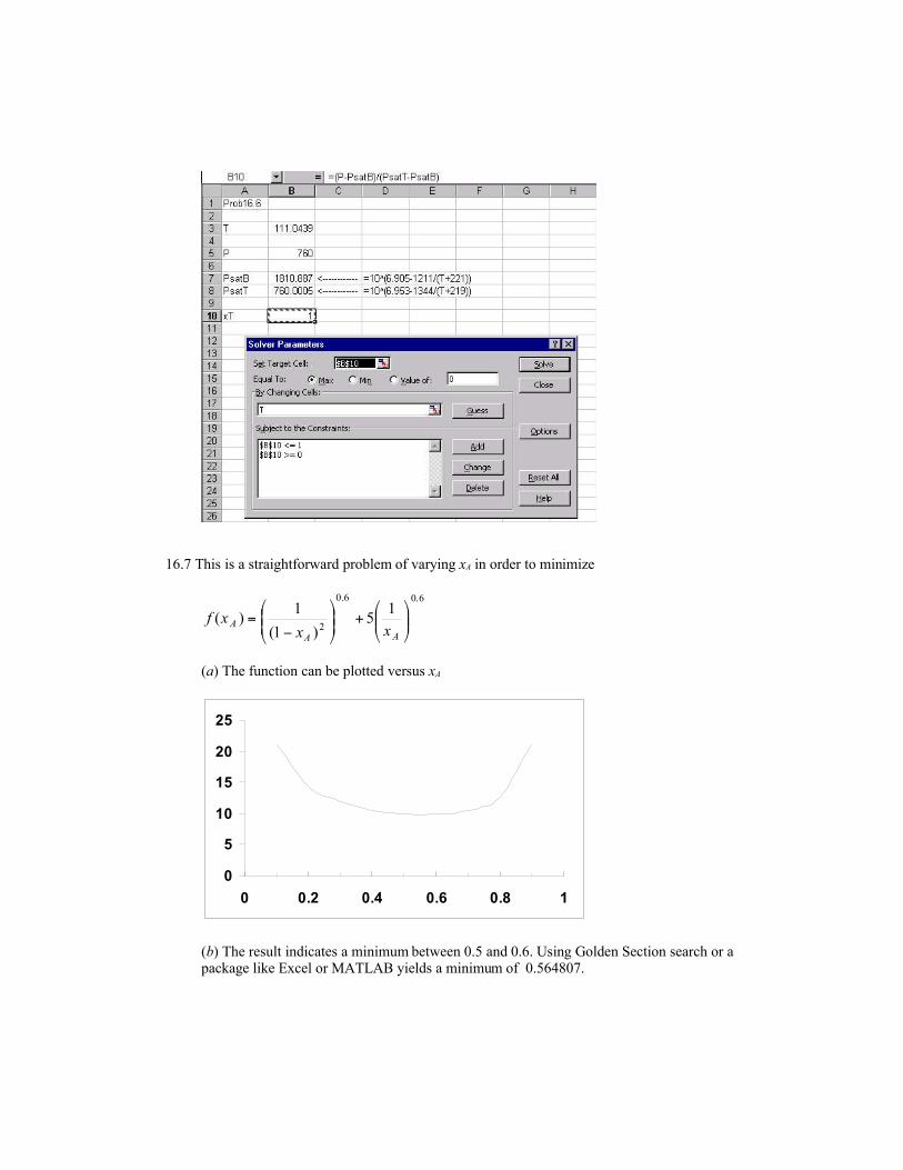
16.7 This is a straightforward problem of varying xA in order to minimize
6.06.0
2
15
)1(
1)(
+
−=
AA
Axx
xf
(a) The function can be plotted versus xA
0
5
10
15
20
25
0 0.2 0.4 0.6 0.8 1
(b) The result indicates a minimum between 0.5 and 0.6. Using Golden Section search or apackage like Excel or MATLAB yields a minimum of 0.564807.

16.8 This is a case of constrained nonlinear optimization. The conversion factors range between 0 and 1. Inaddition, the cost function can not be evaluated for certain combinations of XA1 and XA2. Theproblem is the second term,
( )
6.0
22
2
1
1
1
−
−
A
A
A
x
x
x
If xA1 > xA2, the numerator will be negative and the term cannot be evaluated.
Excel Solver can be used to solve the problem:
The result is

16.9 Errata: Change B0 to 100.
This problem can be set up on Excel and the answer generated with Solver:
The solution is
16.10 The problem can be set up in Excel Solver.

The solution is
16.11
w
d
θ
e
sA
The following formulas can be developed:
2
we = (1)
e
d1tan−=θ (2)
22 eds += (3)
sP 2= (4)
2
wdA =
(5)
Then the following Excel worksheet and Solver application can be set up:

Note that we have named the cells with the labels in the adjacent left columns. Our goal isto minimize the wetted perimeter by varying the depth and width. We apply positivityconstraints along with the constraint that the computed area must equal the desired area.The result is
Thus, this specific application indicates that a 45o angle yields the minimum wettedperimeter.
The verification of whether this result is universal can be attained inductively ordeductively. The inductive approach involves trying several different desired areas inconjunction with our solver solution. As long as the desired area is greater than 0, theresult for the optimal design will be 45o.
The deductive verification involves calculus. The minimum wetted perimeter should occurwhen the derivative of the perimeter with respect to one of the primary dimensions (i.e., wor d) flattens out. That is, the slope is zero. In the case of the width, this would beexpressed by:
0=dw
dP
If the second derivative at this point is positive, the value of w is at a minimum. Toformulate P in terms of w, substitute Eqs. 1 and 5 into 3 to yield
22 )2/()/2( wwAs +=
(6)
Substitute this into Eq. 4 to give
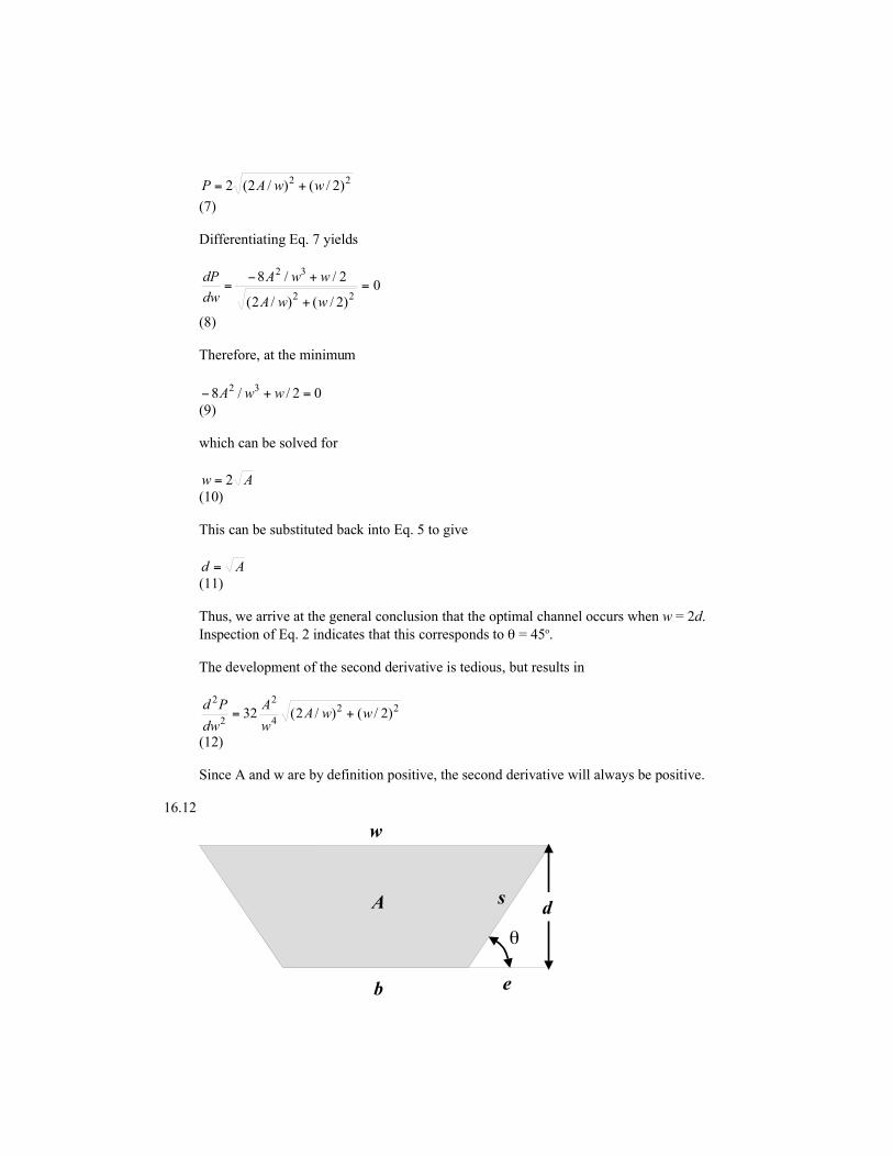
22 )2/()/2(2 wwAP +=
(7)
Differentiating Eq. 7 yields
0
)2/()/2(
2//8
22
32
=+
+−=
wwA
wwA
dw
dP
(8)
Therefore, at the minimum
02//8 32 =+− wwA
(9)
which can be solved for
Aw 2=(10)
This can be substituted back into Eq. 5 to give
Ad =(11)
Thus, we arrive at the general conclusion that the optimal channel occurs when w = 2d.
Inspection of Eq. 2 indicates that this corresponds to θ = 45o.
The development of the second derivative is tedious, but results in
22
4
2
2
2
)2/()/2(32 wwAw
A
dw
Pd+=
(12)
Since A and w are by definition positive, the second derivative will always be positive.
16.12
w
d
θ
b e
sA

The following formulas can be developed:
θtan
de =
(1)
ewb 2−= (2)
22 eds += (3)
bsP += 2 (4)
dbw
A2
+= (5)
Then the following Excel worksheet and Solver application can be set up:
Note that we have named the cells with the labels in the adjacent left columns. Our goal isto minimize the wetted perimeter by varying the depth, width and theta (the angle). Weapply positivity constraints along with the constraint that the computed area must equal thedesired area. We also constrain e that it cannot be greater than w/2. The result is
Thus, this specific application indicates that a 60o angle yields the minimum wettedperimeter.

16.1322 rAends π=
rhAside π2=
sideendstotal AAA +=
hrVcomputed22π=
operateoperatesidesideendsends AFAFAFCost ++=
Then the following Excel worksheet and Solver application can be set up:
which results in the following solution:
16.14 Excel Solver gives: x = 0.5, y = 0.8 and fmin = -0.85.


16.19
2
43
4
)29(100
L
rπ= Lr235 π=
432 )29(.4 rL π= 2
35
rL
π=
2499.1 rL =
mL
mr
08.4
65.1
=
=
16.20 I1 = 4 I2 = 2 I3 = 2 I4 = 0 I5 = 2 P = 80

16.22Total cost is
2102 21 ++= ppC
Total power delivered is
21 4.06.0 ppP +=
Using the Excel Solver:
which yields the solution
16.23 This is a trick question. Because of the presence of (1 – s) in the denominator, the function willexperience a division by zero at the maximum. This can be rectified by merely canceling the (1 – s)terms in the numerator and denominator to give
434
152 +−
=ss
sT
Any of the optimizers described in this section can then be used to determine that the maximum of T= 3 occurs at s = 1.


16.27 An LP formulation for this problem can be set up as
Maximize C X Y Z= + +015 0 025 0 05. . . {Minimize cost}
subject to
X Y Z+ + ≥ 6 {Performance constraint}
X Y+ < 3 {Safety constraint}
X Y− ≥ 0 {X-Y Relationship constraint}
Z Y− ≥0 5 0. {Y-Z Relationship constraint}
(b) An Excel spreadsheet can be set up to solve the problem as
The Solver can be called and set up as
The resulting solution is
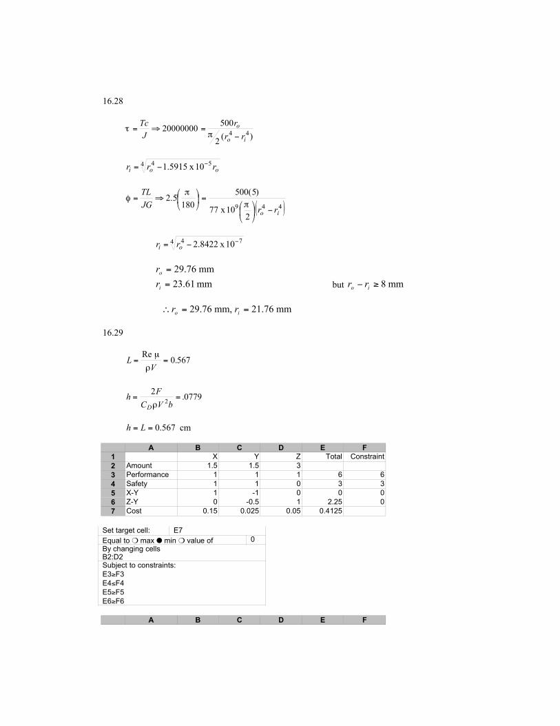
16.28
)(2
50020000000
44io
o
rr
r
J
Tc
−=⇒=π
τ
4 54 10x 5915.1 ooi rrr −−=
( )449
210 x 77
)5(500
1805.2
io rrJG
TL
−
=
⇒=
ππ
φ
4 74 10 x 8422.2 −−= oi rr
mm76.29=or
mm61.23=ir but mm8≥− io rr
mm76.21,mm76.29 ==∴ io rr
16.29
567.0Re
==V
Lρ
µ
0779.2
2==
bVC
Fh
Dρ
567.0== Lh cm
A B C D E F
1 X Y Z Total Constraint
2 Amount 1.5 1.5 3
3 Performance 1 1 1 6 6
4 Safety 1 1 0 3 3
5 X-Y 1 -1 0 0 0
6 Z-Y 0 -0.5 1 2.25 0
7 Cost 0.15 0.025 0.05 0.4125
Set target cell: E7
Equal to ❍ max ● min ❍ value of 0
By changing cellsB2:D2Subject to constraints:E3≥F3E4≤F4E5≥F5E6≥F6
A B C D E F

1 X Y Z Total Constraint
2 Amount 0 0 0
3 Performance 1 1 1 0 6
4 Safety 1 1 0 0 3
5 X-Y 1 -1 0 0 0
6 Z-Y 0 -0.5 1 0 0
7 Cost 0.15 0.025 0.05 0
A B C D E F G
1 Z1 Z2 Z3 W total constraint
2 amount 4000 3500 0 500
3 amount X 1 1 0 0 7500 7500
4 amount Y 2.5 0 1 0 10000 10000
5 amount W 1 -1 -1 -1 0 0
6 profit 2500 -50 200 -300 9675000
Set target cell: F6
Equal to ● max ❍ min ❍ value of 0
By changing cellsB2:E2Subject to constraints:B2≥0C2≥0F3≤G3F4≤G4F5=G5
A B C D E F G
1 Z1 Z2 Z3 W total constraint
2 amount 0 0 0 0
3 amount X 1 1 0 0 0 7500
4 amount Y 2.5 0 1 0 0 10000
5 amount W 1 -1 -1 -1 0 0
6 profit 2500 -50 200 -300 0
Microsoft Excel 5.0c Sensitivity Report
Worksheet: [PROB1605.XLS]Sheet3
Report Created: 12/12/97 9:47
Changing Cells
Final Reduced Objective Allowable Allowable
Cell Name Value Cost Coefficient Increase Decrease
$B$2 amount Product 1 150 0 30 0.833333333 2.5$C$2 amount Product 2 125 0 30 1.666666667 1$D$2 amount Product 3 175 0 35 35 5
Constraints
Final Shadow Constraint Allowable Allowable
Cell Name Value Price R.H. Side Increase Decrease
$E$3 material total 3000 0.625 3000 1E+30 1E+30$E$4 time total 55 12.5 55 1E+30 1E+30$E$5 storage total 450 26.25 450 1E+30 1E+30
A B C D E F
1 Product 1 Product 2 Product 3 total constraint
2 amount 150 125 175
3 material 5 4 10 3000 3000

4 time 0.05 0.1 0.2 55 55
5 storage 1 1 1 450 450
6 profit 30 30 35 14375
Set target cell: E6
Equal to ● max ❍ min ❍ value of 0
By changing cellsB2:D2Subject to constraints:E3≤F3E4≤F4E5≤F5
A B C D E F
1 Product 1 Product 2 Product 3 total constraint
2 amount 0 0 0
3 material 5 4 10 0 3000
4 time 0.05 0.1 0.2 0 55
5 storage 1 1 1 0 450
6 profit 30 30 35 0
Basis P x1 x2 x3 S1 S2 S3 Solution InterceptP 1 -30 -30 -35 0 0 0 0S1 0 5 4 10 1 0 0 3000 300S2 0 0.05 0.1 0.2 0 1 0 55 275S3 0 1 1 1 0 0 1 450 450
Basis P x1 x2 x3 S1 S2 S3 Solution InterceptP 1 -21.25 -12.5 0 0 175 0 9625S1 0 2.5 -1 0 1 -50 0 250 100x3 0 0.25 0.5 1 0 5 0 275 1100S3 0 0.75 0.5 0 0 -5 1 175 233.3333
Basis P x1 x2 x3 S1 S2 S3 Solution InterceptP 1 0 -21 0 8.5 -250 0 11750x1 0 1 -0.4 0 0.4 -20 0 100 -250x3 0 0 0.6 1 -0.1 10 0 250 416.6667S3 0 0 0.8 0 -0.3 10 1 100 125
Basis P x1 x2 x3 S1 S2 S3 SolutionP 1 0 0 0 0.625 12.5 26.25 14375x1 0 1 0 0 0.25 -15 0.5 150x3 0 0 0 1 0.125 2.5 -0.75 175x2 0 0 1 0 -0.375 12.5 1.25 125


A VBA code to do this with the computer is

Sub Splines()Dim i As Integer, n As IntegerDim x(100) As Single, y(100) As Single, xu As Single, yu As SingleDim xint(100) As SingleDim dy As Single, d2y As SingleSheets("Sheet1").SelectRange("a5").Selectn = ActiveCell.RowSelection.End(xlDown).Selectn = ActiveCell.Row - nRange("a5").SelectFor i = 0 To n x(i) = ActiveCell.Value ActiveCell.Offset(0, 1).Select y(i) = ActiveCell.Value ActiveCell.Offset(1, -1).SelectNext iRange("d5").Selectnint = ActiveCell.RowSelection.End(xlDown).Selectnint = ActiveCell.Row - nintRange("d5").SelectFor i = 0 To nint xint(i) = ActiveCell.Value ActiveCell.Offset(1, 0).SelectNext iRange("e5").SelectFor i = 0 To nint Call Spline(x(), y(), n, xint(i), yu, dy, d2y) ActiveCell.Value = yu ActiveCell.Offset(0, 1).Select ActiveCell.Value = dy ActiveCell.Offset(0, 1).Select ActiveCell.Value = d2y ActiveCell.Offset(1, -2).SelectNext iRange("a5").SelectEnd Sub
Sub Spline(x, y, n, xu, yu, dy, d2y)Dim e(10) As Single, f(10) As Single, g(10) As Single, r(10) As Single, d2x(10) As SingleCall Tridiag(x, y, n, e, f, g, r)Call Decomp(e(), f(), g(), n - 1)Call Substit(e(), f(), g(), r(), n - 1, d2x())Call Interpol(x, y, n, d2x(), xu, yu, dy, d2y)End Sub
Sub Tridiag(x, y, n, e, f, g, r)Dim i As Integerf(1) = 2 * (x(2) - x(0))g(1) = x(2) - x(1)r(1) = 6 / (x(2) - x(1)) * (y(2) - y(1))r(1) = r(1) + 6 / (x(1) - x(0)) * (y(0) - y(1))For i = 2 To n - 2 e(i) = x(i) - x(i - 1) f(i) = 2 * (x(i + 1) - x(i - 1)) g(i) = x(i + 1) - x(i) r(i) = 6 / (x(i + 1) - x(i)) * (y(i + 1) - y(i)) r(i) = r(i) + 6 / (x(i) - x(i - 1)) * (y(i - 1) - y(i))Next ie(n - 1) = x(n - 1) - x(n - 2)f(n - 1) = 2 * (x(n) - x(n - 2))r(n - 1) = 6 / (x(n) - x(n - 1)) * (y(n) - y(n - 1))r(n - 1) = r(n - 1) + 6 / (x(n - 1) - x(n - 2)) * (y(n - 2) - y(n - 1))End Sub
Sub Interpol(x, y, n, d2x, xu, yu, dy, d2y)Dim i As Integer, flag As IntegerDim c1 As Single, c2 As Single, c3 As Single, c4 As SingleDim t1 As Single, t2 As Single, t3 As Single, t4 As Singleflag = 0i = 1Do If xu >= x(i - 1) And xu <= x(i) Then

c1 = d2x(i - 1) / 6 / (x(i) - x(i - 1)) c2 = d2x(i) / 6 / (x(i) - x(i - 1)) c3 = y(i - 1) / (x(i) - x(i - 1)) - d2x(i - 1) * (x(i) - x(i - 1)) / 6 c4 = y(i) / (x(i) - x(i - 1)) - d2x(i) * (x(i) - x(i - 1)) / 6 t1 = c1 * (x(i) - xu) ^ 3 t2 = c2 * (xu - x(i - 1)) ^ 3 t3 = c3 * (x(i) - xu) t4 = c4 * (xu - x(i - 1)) yu = t1 + t2 + t3 + t4 t1 = -3 * c1 * (x(i) - xu) ^ 2 t2 = 3 * c2 * (xu - x(i - 1)) ^ 2 t3 = -c3 t4 = c4 dy = t1 + t2 + t3 + t4 t1 = 6 * c1 * (x(i) - xu) t2 = 6 * c2 * (xu - x(i - 1)) d2y = t1 + t2 flag = 1 Else i = i + 1 End If If i = n + 1 Or flag = 1 Then Exit DoLoopIf flag = 0 Then MsgBox "outside range" EndEnd IfEnd Sub
Sub Decomp(e, f, g, n)Dim k As IntegerFor k = 2 To n e(k) = e(k) / f(k - 1) f(k) = f(k) - e(k) * g(k - 1)Next kEnd Sub
Sub Substit(e, f, g, r, n, x)Dim k As IntegerFor k = 2 To n r(k) = r(k) - e(k) * r(k - 1)Next kx(n) = r(n) / f(n)For k = n - 1 To 1 Step -1 x(k) = (r(k) - g(k) * x(k + 1)) / f(k)Next kEnd Sub


20.11 The best fit equation can be determined by nonlinear regression as
][8766.0
][84.98][
F
FB
+=
0
20
40
60
80
100
120
0 10 20 30 40 50 60
Disregarding the point (0, 0), The r2 can be computed as
St = 9902.274Sr = 23.36405
9976.0274.9902
364.23274.99022 =−
=r
20.12 The Excel Solver can be used to develop a nonlinear regression to fit the parameters. Theresult (along with a plot of –dA/dt calculated with the model versus the data estimates) areshown below. Note that the 1:1 line is also displayed on the plot.

20.13 The Excel Solver can be used to develop a nonlinear regression to fit the parameters. Theresult (along with a plot of the model versus the data estimates) are shown below. Note thatthe 1:1 line is also displayed on the plot.
20.14 The standard errors can be computed via Eq. 17.9
2/ −=
n
Ss r
xy
Thus, Model C seems best because its standard error is lower.
20.15 A plot of the natural log of cells versus time indicates two straight lines with a sharp breakat 2. Trendline can be used to fit each range separately with the exponential model asshown in the second plot.
-3
-2
-1
0
1
2
0 2 4 6
y = 0.1000e1.2000x
R2 = 1.0000
y = 0.4953e0.4000x
R2 = 1.0000
0
1
2
3
4
5
6
7
8
0 1 2 3 4 5 6 7
20.16 (This problem was designed by Theresa Good of Texas A&M.) The problem can be solvedwith Microsoft Excel:

20.17Plot the data using Excel:
+
Surface Area vs Weight
y = 0.4149x0.3799
R2 = 0.9711
2.05
2.1
2.15
2.2
2.25
2.3
2.35
60 70 80 90 100
Weight, kg
Su
rfa
ce
Are
a,
sq
ua
red
me
ters
A = 0.4149W0.3799 with R-squared = 0.9711. Therefore, a = 0.4149 and b = 0.3799. The
predicted surface area for a 95 kg human is approximately: A = 0.4149 (95) 0.3799 = 2.34 m2

20.18 The Excel Trend Line tool can be used to fit a power law to the data:
y = 65.768x0.7497
R2 = 0.9935
0
1000
2000
3000
4000
5000
6000
0 100 200 300
The logarithmic slope relating the mass and metabolism is 0.75.
20.19


20.20


20.21 The problem is set up as the following Excel Solver application. Notice that we haveassumed that the model consists of a constant plus two bell-shaped curves:
ππ
)(2
)(1
2221
21
)(axkaxk
ekekcxf
−−−−
++=
The resulting solution is

Thus, the retina thickness is estimated as 0.31 – 0.25 = 0.06.


20.29 Clearly the linear model is not adequate. The second model can be fit with the ExcelSolver:

Notice that we have reexpressed the initial rates by multiplying them by 1×10⁵. We did thisso that the sum of the squares of the residuals would not be miniscule. Sometimes this willlead the Solver to conclude that it is at the minimum, even though the fit is poor. Thesolution is:
Although the fit might appear to be OK, it is biased in that it underestimates the low valuesand overestimates the high ones. The poorness of the fit is really obvious if we display theresults as a log-log plot:
Notice that this view illustrates that the model actually overpredicts the very lowest values.
The third and fourth models provide a means to rectify this problem. Because they raise [S]to powers, they have more degrees of freedom to follow the underlying pattern of the data.For example, the third model gives:

Finally, the cubic model results in a perfect fit:
Thus, the best fit is
][4.0
][104311.2 5
0S
Sv
+
×=
−


20.49 This problem was solved using an Excel spreadsheet.
y = 4E-06x2.6363
R2 = 0.9997
0.0001
0.001
0.01
1 10 100
stress
cre
ep
ra
te
Series1
Power (Series1)
20.50 This problem was solved using an Excel spreadsheet.
y = 0.685x + 2.779R2 = 0.9771
0
1
2
3
4
5
6
7
0 1 2 3 4 5 6
s he a r s t ra i n ra t e
µ = 0.685
τy = 2.779 N/m2

r2 = 0.9771
20.51 This problem was solved using an Excel spreadsheet.
y = 0.7276x0.543
R2 = 0.9891
0
2
4
6
8
10
12
0 20 40 60 80 100 120 140
s he ar s t rai n rat e
µ = 0.7276
n = 0.543
n 15
Model A Model B Model C
Sr 135 90 72
Number of model
parameters fit 2 3 4
sy/x 3.222517 2.738613 2.558409


CHAPTER 13


13.13 Because of multiple local minima and maxima, there is no really simple means to testwhether a single maximum occurs within an interval without actually performing a search.However, if we assume that the function has one maximum and no minima within theinterval, a check can be included. Here is a VBA program to implement the Goldensection search algorithm for maximization and solve Example 13.1.
Option Explicit
Sub GoldMax()Dim ier As IntegerDim xlow As Double, xhigh As DoubleDim xopt As Double, fopt As Doublexlow = 0xhigh = 4Call GoldMx(xlow, xhigh, xopt, fopt, ier)If ier = 0 Then MsgBox "xopt = " & xopt MsgBox "f(xopt) = " & foptElse MsgBox "Does not appear to be maximum in [xl, xu]"End IfEnd Sub
Sub GoldMx(xlow, xhigh, xopt, fopt, ier)Dim iter As Integer, maxit As Integer, ea As Double, es As DoubleDim xL As Double, xU As Double, d As Double, x1 As DoubleDim x2 As Double, f1 As Double, f2 As DoubleConst R As Double = (5 ^ 0.5 - 1) / 2
ier = 0maxit = 50es = 0.001xL = xlowxU = xhighiter = 1d = R * (xU - xL)x1 = xL + dx2 = xU - df1 = f(x1)f2 = f(x2)If f1 > f2 Then xopt = x1 fopt = f1Else xopt = x2 fopt = f2End IfIf fopt > f(xL) And fopt > f(xU) Then Do d = R * d If f1 > f2 Then xL = x2 x2 = x1 x1 = xL + d f2 = f1 f1 = f(x1) Else xU = x1 x1 = x2 x2 = xU - d f1 = f2 f2 = f(x2) End If iter = iter + 1 If f1 > f2 Then

xopt = x1 fopt = f1 Else xopt = x2 fopt = f2 End If If xopt <> 0 Then ea = (1 - R) * Abs((xU - xL) / xopt) * 100 If ea <= es Or iter >= maxit Then Exit Do LoopElse ier = 1End If
End Sub
Function f(x)f = -(2 * Sin(x) - x ^ 2 / 10)End Function
13.14 The easiest way to set up a maximization algorithm so that it can do minimization is therealize that minimizing a function is the same as maximizing its negative. Therefore, thefollowing algorithm minimizes or maximizes depending on the value of a user inputvariable, ind, where ind = -1 and 1 correspond to minimization and maximization,respectively.
Option Explicit
Sub GoldMinMax()Dim ind As Integer 'Minimization (ind = -1); Maximization (ind = 1)Dim xlow As Double, xhigh As DoubleDim xopt As Double, fopt As Doublexlow = 0xhigh = 4Call GoldMnMx(xlow, xhigh, -1, xopt, fopt)MsgBox "xopt = " & xoptMsgBox "f(xopt) = " & foptEnd Sub
Sub GoldMnMx(xlow, xhigh, ind, xopt, fopt)Dim iter As Integer, maxit As Integer, ea As Double, es As DoubleDim xL As Double, xU As Double, d As Double, x1 As DoubleDim x2 As Double, f1 As Double, f2 As DoubleConst R As Double = (5 ^ 0.5 - 1) / 2
maxit = 50es = 0.001xL = xlowxU = xhighiter = 1d = R * (xU - xL)x1 = xL + dx2 = xU - df1 = f(ind, x1)f2 = f(ind, x2)If f1 > f2 Then xopt = x1 fopt = f1Else xopt = x2 fopt = f2End If
Do d = R * d If f1 > f2 Then

xL = x2 x2 = x1 x1 = xL + d f2 = f1 f1 = f(ind, x1) Else xU = x1 x1 = x2 x2 = xU - d f1 = f2 f2 = f(ind, x2) End If iter = iter + 1 If f1 > f2 Then xopt = x1 fopt = f1 Else xopt = x2 fopt = f2 End If If xopt <> 0 Then ea = (1 - R) * Abs((xU - xL) / xopt) * 100 If ea <= es Or iter >= maxit Then Exit DoLoopfopt = ind * foptEnd Sub
Function f(ind, x)f = ind * (1.1333 * x ^ 2 - 6.2667 * x + 1)End Function
13.15 Because of multiple local minima and maxima, there is no really simple means to testwhether a single maximum occurs within an interval without actually performing a search.However, if we assume that the function has one maximum and no minima within theinterval, a check can be included. Here is a VBA program to implement the QuadraticInterpolation algorithm for maximization and solve Example 13.2.
Option Explicit
Sub QuadMax()Dim ier As IntegerDim xlow As Double, xhigh As DoubleDim xopt As Double, fopt As Doublexlow = 0xhigh = 4Call QuadMx(xlow, xhigh, xopt, fopt, ier)If ier = 0 Then MsgBox "xopt = " & xopt MsgBox "f(xopt) = " & foptElse MsgBox "Does not appear to be maximum in [xl, xu]"End IfEnd Sub
Sub QuadMx(xlow, xhigh, xopt, fopt, ier)Dim iter As Integer, maxit As Integer, ea As Double, es As DoubleDim x0 As Double, x1 As Double, x2 As DoubleDim f0 As Double, f1 As Double, f2 As DoubleDim xoptOld As Double
ier = 0maxit = 50es = 0.01x0 = xlowx2 = xhighx1 = (x0 + x2) / 2

f0 = f(x0)f1 = f(x1)f2 = f(x2)If f1 > f0 Or f1 > f2 Then xoptOld = x1 Do xopt = f0 * (x1^2 - x2^2) + f1 * (x2^2 - x0^2) + f2 * (x0^2 - x1^2) xopt = xopt / (2*f0 * (x1 - x2) + 2*f1 * (x2 - x0) + 2*f2 * (x0 - x1)) fopt = f(xopt) iter = iter + 1 If xopt > x1 Then x0 = x1 f0 = f1 x1 = xopt f1 = fopt Else x2 = x1 f2 = f1 x1 = xopt f1 = fopt End If If xopt <> 0 Then ea = Abs((xopt - xoptOld) / xopt) * 100 xoptOld = xopt If ea <= es Or iter >= maxit Then Exit Do LoopElse ier = 1End IfEnd Sub
Function f(x)f = -(2 * Sin(x) - x ^ 2 / 10)End Function
13.16 Here is a VBA program to implement the Newton-Raphson method for maximization. Option Explicit
Sub NRMax()Dim xguess As DoubleDim xopt As Double, fopt As Doublexguess = 2.5Call NRMx(xguess, xopt, fopt)MsgBox "xopt = " & xoptMsgBox "f(xopt) = " & foptEnd Sub
Sub NRMx(xguess, xopt, fopt)Dim iter As Integer, maxit As Integer, ea As Double, es As DoubleDim x0 As Double, x1 As Double, x2 As DoubleDim f0 As Double, f1 As Double, f2 As DoubleDim xoptOld As Double
maxit = 50es = 0.01Do xopt = xguess - df(xguess) / d2f(xguess) fopt = f(xopt) If xopt <> 0 Then ea = Abs((xopt - xguess) / xopt) * 100 xguess = xopt If ea <= es Or iter >= maxit Then Exit DoLoopEnd Sub
Function f(x)f = -(2 * Sin(x) - x ^ 2 / 10)

End Function
Function df(x)df = 2 * Cos(x) - x / 5End Function
Function d2f(x)d2f = -2 * Sin(x) - 1 / 5End Function
13.17 Here is a VBA program to implement the Newton-Raphson method for maximization.
( ) 23606.1242
151 =−
−=d
23606.32 11 =+= dx
76394.24 12 =−= dx
69808.4)( 1 −=xf
55333.5)( 2 −=xf
Uxnewisxxfxf 112 )()( ⇒<
( ) 763927.0223606.32
152 =−
−=d
7639.22 21 =+= dx
472133.223606.3 22 =−= dx
55331.5)( 1 −=xf
82656.4)( 2 −=xf
221 )()( xxfxf ⇒< is new Lx
( ) 4721.0472133.223606.32
153 =−
−=d
9442.2472133.2 31 =+= dx
7639.223606.3 32 =−= dx
9353.4)( 1 −=xf
55331.5)( 2 −=xf
112 )()( xxfxf ⇒< is new Ux
( ) 29175.0472133.29442.22
154 =−
−=d
7638.2472133.2 41 =+= dx
6524.29442.2 42 =−= dx
55331.5)( 1 −=xf
4082.5)( 2 −=xf
∴ at time 76.2=t , minimum pressure is –5.55331

CHAPTER 14
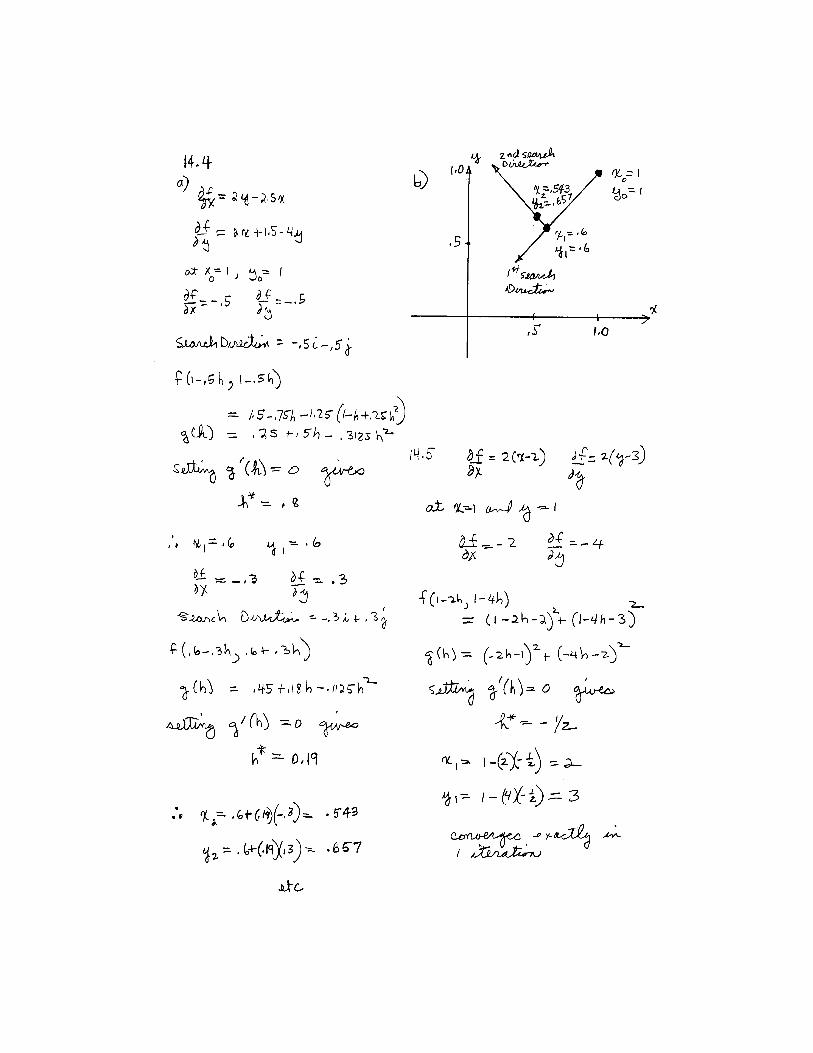
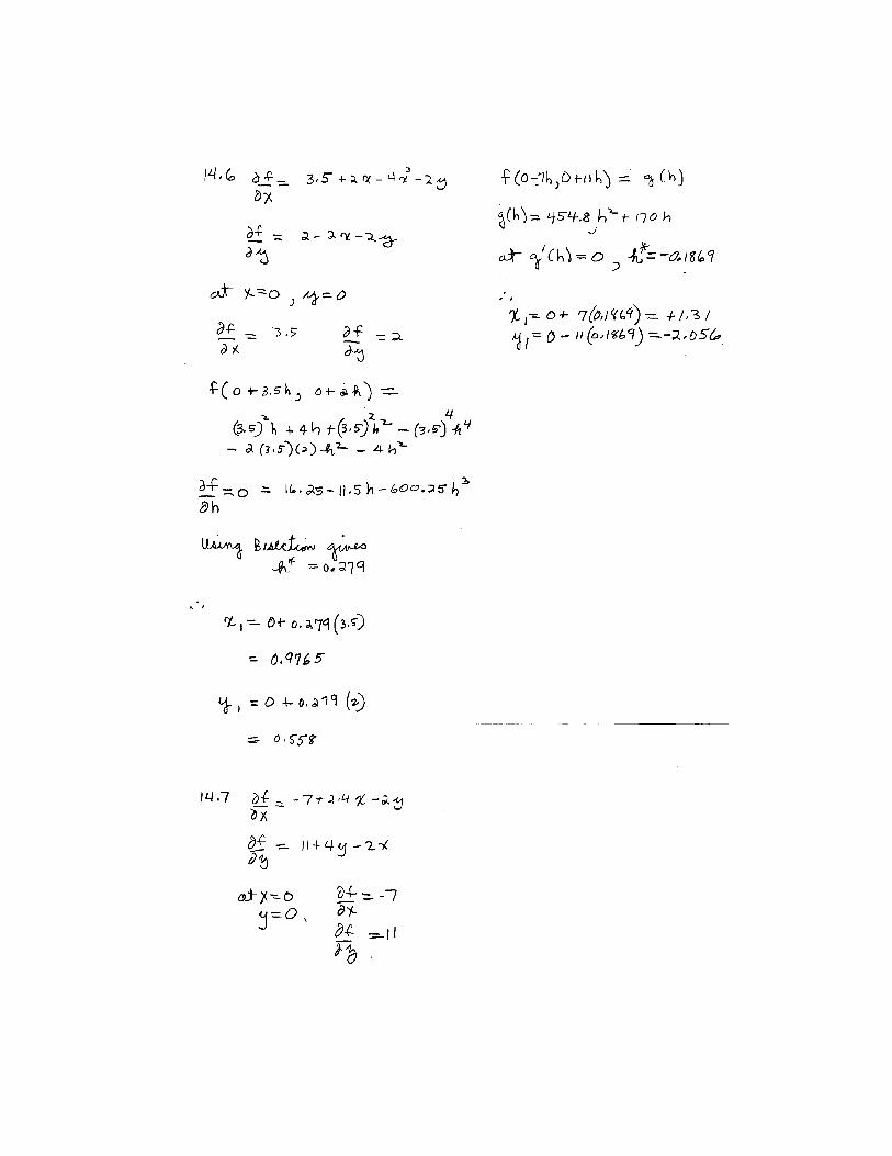

14.8 Errata: p. 357; The initial value of the variable maxf must be set to some ridiculously
small value before the iterations are begun. Add the following line to the beginning of
the VBA code:
maxf = -999E9
The following code implements the random search algorithm in VBA:
Option ExplicitSub RandSearch()
Dim n As LongDim xmin As Single, xmax As Single, ymin As Single, ymax As SingleDim maxf As Single, maxx As Single, maxy As Single
xmin = -2xmax = 2ymin = -2ymax = 2
n = InputBox("n=")Call RndSrch(n, xmin, xmax, ymin, ymax, maxy, maxx, maxf)
MsgBox maxfMsgBox maxxMsgBox maxy
End SubSub RndSrch(n, xmin, xmax, ymin, ymax, maxy, maxx, maxf)Dim j As LongDim x As Single, y As Single, fn As Singlemaxf = -999E9For j = 1 To n x = xmin + (xmax - xmin) * Rnd y = ymin + (ymax - ymin) * Rnd fn = f(x, y) If fn > maxf Then maxf = fn maxx = x maxy = y End IfNext jEnd Sub
Function f(x, y)f = 3.5 * x + 2 * y + x ^ 2 - x ^ 4 - 2 * x * y - y ^ 2End Function
14.9 The following code implements the grid search algorithm in VBA:
Option ExplicitSub GridSearch()
Dim nx As Long, ny As LongDim xmin As Single, xmax As Single, ymin As Single, ymax As SingleDim maxf As Single, maxx As Single, maxy As Single
xmin = -2xmax = 2ymin = -2ymax = 2nx = 1000ny = 1000

Call GridSrch(nx, ny, xmin, xmax, ymin, ymax, maxy, maxx, maxf)
MsgBox maxfMsgBox maxxMsgBox maxy
End SubSub GridSrch(nx, ny, xmin, xmax, ymin, ymax, maxy, maxx, maxf)Dim i As Long, j As LongDim x As Single, y As Single, fn As SingleDim xinc As Single, yinc As Singlexinc = (xmax - xmin) / nxyinc = (ymax - ymin) / nymaxf = -999000000000#x = xminFor i = 0 To nx y = ymin For j = 0 To ny fn = f(x, y) If fn > maxf Then maxf = fn maxx = x maxy = y End If y = y + yinc Next j x = x + xincNext iEnd Sub
Function f(x, y)f = y - x - 2 * x ^ 2 - 2 * x * y - y ^ 2End Function
14.10
222 785),( xyyxyxf −−=
24)4(14)4)(2(101410 =−⇒−=∂∂
xxyx
f
48)2(16)4(5165 22 =−⇒−=∂∂
yxy
f
jif ˆ48ˆ24 +=∇
)482,244(, hhfhy
fyh
x
fxf oo ++=
∂∂
+∂∂
+
= 222 )244(7)482(8)482()244(5 hhhh +−+−++
16288029376138240)( 23 +++= hhhxg

14.11
yxyxyxyxf 462),( 223 ++−=
2)1(2)1(6)1)(1(6266 22 =+−⇒+−=∂∂
xyyxx
f
24)1(6)1)(1(4464 3 =+−⇒+−=∂∂
yyxx
f
jif ˆ2ˆ2 +=∇
)21,21()2
2,
2
2( hhfh
y
fyh
x
fxf oo ++=++
)21(4)21()21)(21(6)21()21(2 223 hhhhhh ++++++−++=
186016016064)( 2345 +++++= hhhhhxg

CHAPTER 15
15.1 (Note: Although it is not really clear from the problem statement, it should be assumed that eachunit of product is equivalent to a kg.)
(a) Define xa = amount of product A produced, and xb = amount of product B produced.The objective function is to maximize profit,
P x xa b= +45 30
Subject to the following constraints
20 5 10000x xa b+ ≤ {raw materials}
0 05 015 40. .x xa b+ ≤ {production time}
x xa b+ ≤ 550 {storage}
x xa b, ≥ 0 {positivity}
(b) To solve graphically, the constraints can be reformulated as the following straight lines
x xb a= −2000 4 {raw materials}
x xb a= −266 667 0 3333. . {production time}
x xb a= −550 {storage}
The objective function can be reformulated as
x P xb a= −( / ) .1 30 15
The constraint lines can be plotted on the xb-xa plane to define the feasible space. Then theobjective function line can be superimposed for various values of P until it reaches the
boundary. The result is P ≅ 23700 with xa ≅ 483 and xb ≅ 67. Notice also that material andstorage are the binding constraints and that there is some slack in the time constraint.

0
100
200
300
0 200 400 600
P =
15000
P =
5000
P =
23700
xb
xa
time
storag
e
mate
rial
optimum
(c) The simplex tableau for the problem can be set up and solved as
Basis P xa xb S1 S2 S3 Solution InterceptP 1 -45 -30 0 0 0 0
material S1 0 20 5 1 0 0 10000 500time S2 0 0.05 0.15 0 1 0 40 800storage S3 0 1 1 0 0 1 550 550
Basis P xa xb S1 S2 S3 Solution InterceptP 1 0 -18.75 2.25 0 0 22500
xa xa 0 1 0.25 0.05 0 0 500 2000time S2 0 0 0.1375 -0 1 0 15 109.0909storage S3 0 0 0.75 -0.05 0 1 50 66.66667
Basis P xa xb S1 S2 S3 Solution InterceptP 1 0 0 1 0 25 23750
xa xa 0 1 0 0.067 0 -0.333 483.33333time S2 0 0 0 0.007 1 -0.183 5.8333333xb xb 0 0 1 -0.07 0 1.333 66.666667
(d) An Excel spreadsheet can be set up to solve the problem as
A B C D E1 xA xB total constraint2 amount 0 03 time 0.05 0.15 0 404 storage 1 1 0 5505 raw material 20 5 0 100006 profit 45 30 0
The Solver can be called and set up as
Set target cell: D6
Equal to ● max ❍ min ❍ value of 0

By changing cellsB2:C2Subject to constraints:D3≤E3D4≤E4D5≤E5
The resulting solution is
A B C D E1 xA xB total constraint2 amount 483.3333 66.666673 time 0.05 0.15 34.16667 404 storage 1 1 550 5505 raw material 20 5 10000 100006 profit 45 30 23750
In addition, a sensitivity report can be generated as
Microsoft Excel 5.0c Sensitivity Report
Worksheet: [PROB1501.XLS]Sheet2
Report Created: 12/8/97 17:06
Changing Cells
Final Reduced Objective Allowable AllowableCell Name Value Cost Coefficient Increase Decrease
$B$2 amount xA 483.3333333 0 45 75 15$C$2 amount xB 66.66666667 0 30 15 18.75
Constraints
Final Shadow Constraint Allowable AllowableCell Name Value Price R.H. Side Increase Decrease
$D$3 time 34.16666667 0 40 1E+30 5.833333333$D$4 storage 550 25 550 31.81818182 1E+30$D$5 raw material 10000 1 10000 1E+30 875
(e) The high shadow price for storage from the sensitivity analysis from (d) suggests thatincreasing storage will result in the best increase in profit.
15.2 (a) The total LP formulation is given by
Maximize Z x x x= + +150 175 2501 2 3 {Maximize profit}
subject to
7 11 15 1541 2 3x x x+ + ≤ {Material constraint}
10 8 12 801 2 3x x x+ + ≤ {Time constraint}
x1 9≤ {“Regular” storage constraint}
x2 6≤ {“Premium” storage constraint}
x2 5≤ {“Supreme” storage constraint}
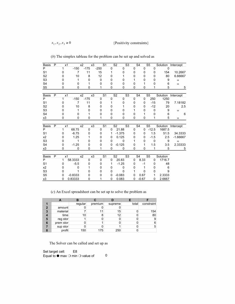
x x x1 2 3 0, , ≥ {Positivity constraints}
(b) The simplex tableau for the problem can be set up and solved as
Basis P x1 x2 x3 S1 S2 S3 S4 S5 Solution InterceptP 1 -150 -175 -250 0 0 0 0 0 0S1 0 7 11 15 1 0 0 0 0 154 10.2667S2 0 10 8 12 0 1 0 0 0 80 6.66667S3 0 1 0 0 0 0 1 0 0 9 ∞S4 0 0 1 0 0 0 0 1 0 6 ∞S5 0 0 0 1 0 0 0 0 1 5 5
Basis P x1 x2 x3 S1 S2 S3 S4 S5 Solution InterceptP 1 -150 -175 0 0 0 0 0 250 1250S1 0 7 11 0 1 0 0 0 -15 79 7.18182S2 0 10 8 0 0 1 0 0 -12 20 2.5S3 0 1 0 0 0 0 1 0 0 9 ∞S4 0 0 1 0 0 0 0 1 0 6 6x3 0 0 0 1 0 0 0 0 1 5 ∞
Basis P x1 x2 x3 S1 S2 S3 S4 S5 Solution InterceptP 1 68.75 0 0 0 21.88 0 0 -12.5 1687.5S1 0 -6.75 0 0 1 -1.375 0 0 1.5 51.5 34.3333x2 0 1.25 1 0 0 0.125 0 0 -1.5 2.5 -1.66667S3 0 1 0 0 0 0 1 0 0 9 ∞S4 0 -1.25 0 0 0 -0.125 0 1 1.5 3.5 2.33333x3 0 0 0 1 0 0 0 0 1 5 5
Basis P x1 x2 x3 S1 S2 S3 S4 S5 SolutionP 1 58.3333 0 0 0 20.83 0 8.33 0 1716.7S1 0 -5.5 0 0 1 -1.25 0 -1 0 48x2 0 0 1 0 0 0 0 1 0 6S3 0 1 0 0 0 0 1 0 0 9S5 0 -0.8333 0 0 0 -0.083 0 0.67 1 2.3333x3 0 0.83333 0 1 0 0.083 0 -0.67 0 2.6667
(c) An Excel spreadsheet can be set up to solve the problem as
A B C D E F
1 regular premium supreme total constraint
2 amount 0 0 0
3 material 7 11 15 0 154
4 time 10 8 12 0 80
5 reg stor 1 0 0 0 9
6 prem stor 0 1 0 0 6
7 sup stor 0 0 1 0 5
8 profit 150 175 250 0
The Solver can be called and set up as
Set target cell: E8
Equal to ● max ❍ min ❍ value of 0

By changing cellsB2:D2Subject to constraints:E3≤F3E4≤F4E5≤F5E6≤F6E7≤F7B2≥0C2≥0D2≥0
The resulting solution is
A B C D E F
1 regular premium supreme total constraint
2 amount 0 6 2.666667
3 material 7 11 15 106 154
4 time 10 8 12 80 80
5 reg stor 1 0 0 0 9
6 prem stor 0 1 0 6 6
7 sup stor 0 0 1 2.666667 5
8 profit 150 175 250 1716.667
In addition, a sensitivity report can be generated as
Microsoft Excel 5.0c Sensitivity Report
Worksheet: [PROB1502.XLS]Sheet4
Report Created: 12/12/97 9:53
Changing Cells
Final Reduced Objective Allowable AllowableCell Name Value Cost Coefficient Increase Decrease
$B$2 amount regular 0 -58.33333333 150 58.33333333 1E+30$C$2 amount premium 6 0 175 1E+30 8.333333333$D$2 amount supreme 2.666666667 0 250 12.5 70
Constraints
Final Shadow Constraint Allowable AllowableCell Name Value Price R.H. Side Increase Decrease
$E$3 material total 106 0 154 1E+30 48$E$4 time total 80 20.83333333 80 28 32$E$5 reg stor total 0 0 9 1E+30 9$E$6 prem stor total 6 8.333333333 6 4 3.5$E$7 sup stor total 2.666666667 0 5 1E+30 2.333333333
(d) The high shadow price for time from the sensitivity analysis from (c) suggests thatincreasing time will result in the best increase in profit.


(c) Using the Excel Solver


(c) Using the Excel Solver


15.11
Total surface area =
+
42
2D
DHπ
π
Minimize2
),(2D
DHHDfπ
π +=
Constraints:
102
103
3204
2
≤≤
≤≤
≥
H
D
HDπ
243.407
2
DH
D
D
AH
=
−=π
6.96cmD
8.41cmH
cm260when 2
=
=
≈A
15.12
Profit: 21 000,15000,13 xxz +=
Constraints: 1. 8000215.17 21 ≤+ xx
2. 240000500680 21 ≤+ xx
3. 4001 ≤x
4. 3502 ≤x
5,6. 0, 21 ≤xx
$5,810,000z
cars1.188x
cars2.224
1
2
=
=
=x


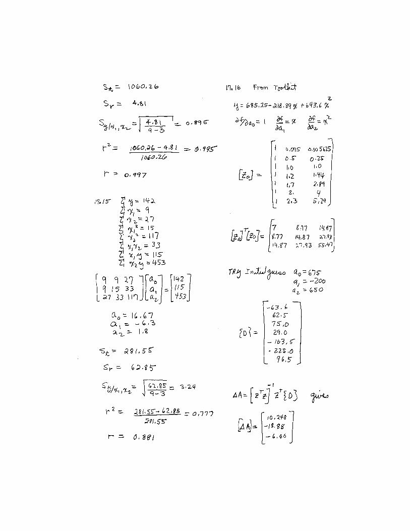


17.19 Here’s VBA code to implement linear regression:
Option Explicit
Sub Regres()
Dim n As IntegerDim x(20) As Single, y(20) As Single, a1 As Single, a0 As SingleDim syx As Single, r2 As Single
n = 7x(1) = 1: x(2) = 2: x(3) = 3: x(4) = 4: x(5) = 5x(6) = 6: x(7) = 7y(1) = 0.5: y(2) = 2.5: y(3) = 2: y(4) = 4: y(5) = 3.5y(6) = 6: y(7) = 5.5
Call Linreg(x(), y(), n, a1, a0, syx, r2)MsgBox "slope= " & a1MsgBox "intercept= " & a0MsgBox "standard error= " & syxMsgBox "coefficient of determination= " & r2MsgBox "correlation coefficient= " & Sqr(r2)
End Sub
Sub Linreg(x, y, n, a1, a0, syx, r2)
Dim i As IntegerDim sumx As Single, sumy As Single, sumxy As SingleDim sumx2 As Single, st As Single, sr As SingleDim xm As Single, ym As Single
sumx = 0sumy = 0sumxy = 0sumx2 = 0st = 0sr = 0For i = 1 To n sumx = sumx + x(i) sumy = sumy + y(i) sumxy = sumxy + x(i) * y(i) sumx2 = sumx2 + x(i) ^ 2Next ixm = sumx / nym = sumy / na1 = (n * sumxy - sumx * sumy) / (n * sumx2 - sumx * sumx)a0 = ym - a1 * xmFor i = 1 To n st = st + (y(i) - ym) ^ 2 sr = sr + (y(i) - a1 * x(i) - a0) ^ 2Next isyx = (sr / (n - 2)) ^ 0.5r2 = (st - sr) / st
End Sub

17.20
log N log Stress
0 3.053463
1 3.024486
2 2.996949
3 2.903633
4 2.813581
5 2.749736
6 2.630428
n =7
∑ = 514.58ii yx
∑ = 912ix
∑ = 21ix
∑ = 17228.20iy
8817.2
3
=
=
y
x
07153.0)21()91(7
)17228.20)(21()514.58(7
)( 2221 −=−
−=
−
−=∑ ∑
∑∑ii
iiii
xxn
yxyxna
09629.3)3)(07153.0(8817.21 =−−=−= xayao
Therefore, 0963.307153.0 +−= xy . Excel spreadsheet solution:
least squares fit
y = -0.0715x + 3.0963
R2 = 0.9617
2.6
2.7
2.8
2.9
3
3.1
3.2
0 1 2 3 4 5 6 7
log cycles
log
str
ess
Series1
Linear (Series1)

17.21 This problem was solved using an Excel spreadsheet and TrendLine. Linear regressiongives
y = 0.0454x + 0.1077
R2 = 0.999
0
0.2
0.4
0.6
0 2 4 6 8 10
Forcing a zero intercept yields
y = 0.061x
R2 = 0.8387
0
0.2
0.4
0.6
0 2 4 6 8 10
One alternative that would force a zero intercept is a power fit
y = 0.1827x0.4069
R2 = 0.9024
0
0.2
0.4
0.6
0 2 4 6 8 10
However, this seems to represent a poor compromise since it misses the linear trend in the data.An alternative approach would to assume that the physically-unrealistic non-zero intercept is anartifact of the measurement method. Therefore, if the linear slope is valid, we might try y =0.0454x.

17.22 This problem was solved using an Excel spreadsheet.
y = -3.7409x + 7.3503
R2 = 0.9908
-3.5
-3
-2.5
-2
-1.5
-1
-0.5
0
0.5
0 0.5 1 1.5 2 2.5 3
l o g t e mp
17.23 Using Excel, plot a linear fit which results in R2 = 0.9949. Using an exponential fit resultsin R2 = 1, which implies a perfect fit. Therefore, use the exponential solution.
The amount of bacteria after 30 days:
6
0257.0
1067.145)30(
382.67
×=
=
y
eyx

Amount of Bacteria Present over a Specified Number of Days
y = 2.2529x + 65.721
R2 = 0.9949
0
20
40
60
80
100
120
0 5 10 15 20 25
Days
Am
ou
nt
Amount of Bacteria Present over a Specified Number of Days
y = 67.382e0.0257x
R2 = 1
0
20
40
60
80
100
120
0 5 10 15 20 25
Days
Am
ou
nt

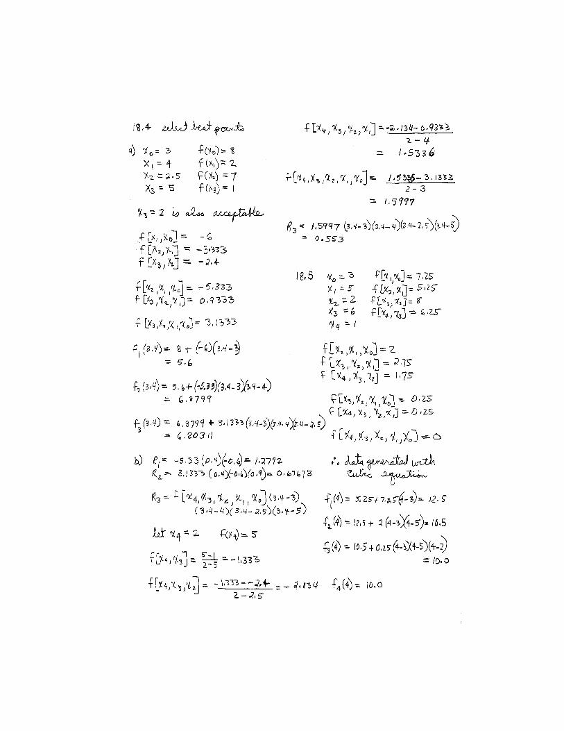


18.14 Here is a VBA program to implement Newton interpolation. It is set up to solve Example18.5:
Option Explicit
Sub Newt()
Dim n As Integer, i As IntegerDim yint(10) As Single, x(10) As Single, y(10) As SingleDim ea(10) As Single, xi As Single
Range("a5").Selectn = ActiveCell.RowSelection.End(xlDown).Selectn = ActiveCell.Row - nRange("a5").SelectFor i = 0 To n x(i) = ActiveCell.Value ActiveCell.Offset(0, 1).Select y(i) = ActiveCell.Value ActiveCell.Offset(1, -1).SelectNext iRange("e3").Selectxi = ActiveCell.Value

Call Newtint(x(), y(), n, xi, yint, ea)
Sheets("Sheet1").SelectRange("d5:f25").ClearContentsRange("d5").SelectFor i = 0 To n ActiveCell.Value = i ActiveCell.Offset(0, 1).Select ActiveCell.Value = yint(i) ActiveCell.Offset(0, 1).Select ActiveCell.Value = ea(i) ActiveCell.Offset(1, -2).SelectNext iRange("a5").Select
End Sub
Sub Newtint(x, y, n, xi, yint, ea)
Dim i As Integer, j As Integer, order As IntegerDim fdd(10, 10) As Single, xterm As SingleDim yint2 As Single
For i = 0 To n fdd(i, 0) = y(i)Next iFor j = 1 To n For i = 0 To n - j fdd(i, j) = (fdd(i + 1, j - 1) - fdd(i, j - 1)) / (x(i + j) - x(i)) Next iNext jxterm = 1#yint(0) = fdd(0, 0)For order = 1 To n xterm = xterm * (xi - x(order - 1)) yint2 = yint(order - 1) + fdd(0, order) * xterm ea(order - 1) = yint2 - yint(order - 1) yint(order) = yint2Next order
End Sub
18.15 Here is the solution when the program from Prob. 18.14 is run.
18.16 See solutions for Probs. 18.1 through 18.3.
18.17 A plot of the error can easily be added to the Excel application. The following shows thesolution for Prob. 18.4:

The following shows the solution for Prob. 18.5:
18.18Option Explicit
Sub LagrInt()
Dim n As Integer, i As Integer, order As IntegerDim x(10) As Single, y(10) As Single, xi As Single
Range("a5").Selectn = ActiveCell.RowSelection.End(xlDown).Selectn = ActiveCell.Row - nRange("a5").SelectFor i = 0 To n x(i) = ActiveCell.Value ActiveCell.Offset(0, 1).Select y(i) = ActiveCell.Value ActiveCell.Offset(1, -1).SelectNext iRange("e3").Selectorder = ActiveCell.ValueActiveCell.Offset(1, 0).Selectxi = ActiveCell.Value

ActiveCell.Offset(2, 0).SelectActiveCell.Value = Lagrange(x(), y(), order, xi)
End Sub
Function Lagrange(x, y, order, xi)
Dim i As Integer, j As IntegerDim sum As Single, prod As Single
sum = 0#For i = 0 To order prod = y(i) For j = 0 To order If i <> j Then prod = prod * (xi - x(j)) / (x(i) - x(j)) End If Next j sum = sum + prodNext iLagrange = sum
End Function
Application to Example 18.7:
18.19 The following VBA program uses cubic interpolation for all intervals:
Option Explicit
Sub Newt()
Dim n As Integer, i As IntegerDim yint(10) As Single, x(10) As Single, y(10) As SingleDim ea(10) As Single, xi As Single
Range("a5").Selectn = ActiveCell.RowSelection.End(xlDown).Selectn = ActiveCell.Row - nRange("a5").SelectFor i = 0 To n x(i) = ActiveCell.Value ActiveCell.Offset(0, 1).Select y(i) = ActiveCell.Value ActiveCell.Offset(1, -1).SelectNext iRange("e4").Selectxi = ActiveCell.Value
ActiveCell.Offset(2, 0).SelectActiveCell.Value = Interp(x(), y(), n, xi)Range("a5").Select

End Sub
Function Interp(x, y, n, xx)
Dim ii As Integer
If xx < x(0) Or xx > x(n) Then Interp = "out of range"Else If xx <= x(ii + 1) Then Interp = Lagrange(x, y, 0, 3, xx) ElseIf xx <= x(n - 1) Then For ii = 0 To n - 2 If xx >= x(ii) And xx <= x(ii + 1) Then Interp = Lagrange(x, y, ii - 1, 3, xx) Exit For End If Next ii Else Interp = Lagrange(x, y, n - 3, 3, xx) End IfEnd IfEnd Function
Function Lagrange(x, y, i0, order, xi)
Dim i As Integer, j As IntegerDim sum As Single, prod As Single
sum = 0#For i = i0 To i0 + order prod = y(i) For j = i0 To i0 + order If i <> j Then prod = prod * (xi - x(j)) / (x(i) - x(j)) End If Next j sum = sum + prodNext iLagrange = sum
End Function
Application to evaluate ln(2.5):
18.20Sub Splines()Dim i As Integer, n As Integer

Dim x(7) As Single, y(7) As Single, xu As Single, yu As SingleDim dy As Single, d2y As Single
Range("a5").Selectn = ActiveCell.RowSelection.End(xlDown).Selectn = ActiveCell.Row - nRange("a5").SelectFor i = 0 To n x(i) = ActiveCell.Value ActiveCell.Offset(0, 1).Select y(i) = ActiveCell.Value ActiveCell.Offset(1, -1).SelectNext iRange("e4").Selectxu = ActiveCell.Value
Call Spline(x(), y(), n, xu, yu, dy, d2y)
ActiveCell.Offset(2, 0).SelectActiveCell.Value = yu
End Sub
Sub Spline(x, y, n, xu, yu, dy, d2y)Dim e(10) As Single, f(10) As Single, g(10) As Single, r(10) As Single,d2x(10) As Single
Call Tridiag(x, y, n, e, f, g, r)Call Decomp(e(), f(), g(), n - 1)Call Substit(e(), f(), g(), r(), n - 1, d2x())Call Interpol(x, y, n, d2x(), xu, yu, dy, d2y)
End Sub
Sub Tridiag(x, y, n, e, f, g, r)Dim i As Integer
f(1) = 2 * (x(2) - x(0))g(1) = x(2) - x(1)r(1) = 6 / (x(2) - x(1)) * (y(2) - y(1))r(1) = r(1) + 6 / (x(1) - x(0)) * (y(0) - y(1))For i = 2 To n - 2 e(i) = x(i) - x(i - 1) f(i) = 2 * (x(i + 1) - x(i - 1)) g(i) = x(i + 1) - x(i) r(i) = 6 / (x(i + 1) - x(i)) * (y(i + 1) - y(i)) r(i) = r(i) + 6 / (x(i) - x(i - 1)) * (y(i - 1) - y(i))Next ie(n - 1) = x(n - 1) - x(n - 2)f(n - 1) = 2 * (x(n) - x(n - 2))r(n - 1) = 6 / (x(n) - x(n - 1)) * (y(n) - y(n - 1))r(n - 1) = r(n - 1) + 6 / (x(n - 1) - x(n - 2)) * (y(n - 2) - y(n - 1))
End Sub
Sub Interpol(x, y, n, d2x, xu, yu, dy, d2y)Dim i As Integer, flag As IntegerDim c1 As Single, c2 As Single, c3 As Single, c4 As SingleDim t1 As Single, t2 As Single, t3 As Single, t4 As Single
flag = 0i = 1Do If xu >= x(i - 1) And xu <= x(i) Then c1 = d2x(i - 1) / 6 / (x(i) - x(i - 1)) c2 = d2x(i) / 6 / (x(i) - x(i - 1))
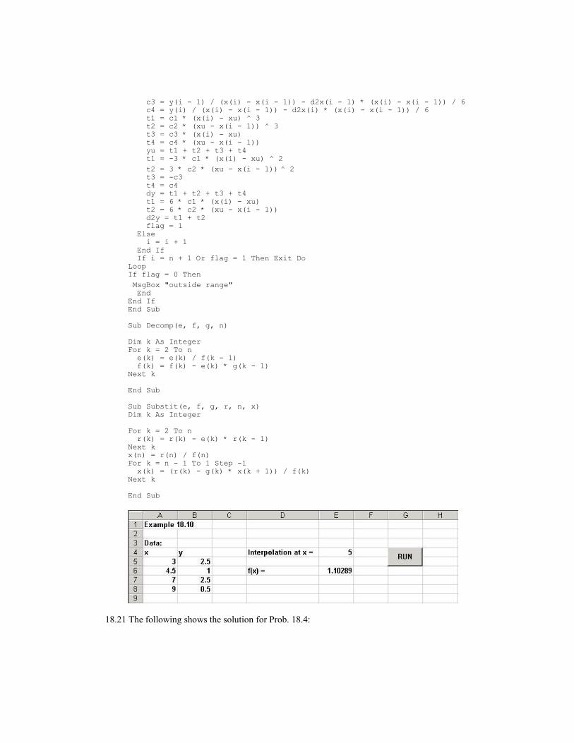
c3 = y(i - 1) / (x(i) - x(i - 1)) - d2x(i - 1) * (x(i) - x(i - 1)) / 6 c4 = y(i) / (x(i) - x(i - 1)) - d2x(i) * (x(i) - x(i - 1)) / 6 t1 = c1 * (x(i) - xu) ^ 3 t2 = c2 * (xu - x(i - 1)) ^ 3 t3 = c3 * (x(i) - xu) t4 = c4 * (xu - x(i - 1)) yu = t1 + t2 + t3 + t4 t1 = -3 * c1 * (x(i) - xu) ^ 2
t2 = 3 * c2 * (xu - x(i - 1)) ^ 2 t3 = -c3 t4 = c4 dy = t1 + t2 + t3 + t4 t1 = 6 * c1 * (x(i) - xu) t2 = 6 * c2 * (xu - x(i - 1)) d2y = t1 + t2 flag = 1 Else i = i + 1 End If If i = n + 1 Or flag = 1 Then Exit DoLoopIf flag = 0 Then
MsgBox "outside range" EndEnd IfEnd Sub
Sub Decomp(e, f, g, n)
Dim k As IntegerFor k = 2 To n e(k) = e(k) / f(k - 1) f(k) = f(k) - e(k) * g(k - 1)Next k
End Sub
Sub Substit(e, f, g, r, n, x)Dim k As Integer
For k = 2 To n r(k) = r(k) - e(k) * r(k - 1)Next kx(n) = r(n) / f(n)For k = n - 1 To 1 Step -1 x(k) = (r(k) - g(k) * x(k + 1)) / f(k)Next k
End Sub
18.21 The following shows the solution for Prob. 18.4:

The following shows the solution for Prob. 18.5:
18.22
Kkg
kJs
xfx
xxf
xxf
xxxx
xfxfxfxf o
o
oo
6487.6
6487.6)(,118.0
579.15789107.4)(
)11144.0(11144.012547.0
5453.67664.65453.6)(
)()()(
)()(
1
1
1
1
11
=
==
+=
−
−
−+=
−−−
+=

CHAPTER 19
19.1 The normal equations can be derived as
11 2 416183 2 0180982 416183 6 004565 0 0170372 018098 0 017037 4 995435
83 915439341081054
0
1
1
. .. . .. . .
...
=
A
A
B
which can be solved for
A0 = 7.957538A1 = -0.6278B1 = -1.04853
The mean is 7.958 and the amplitude and the phase shift can be computed as
C12 2
1
0 6278 104853 1222
104853
0 62782 11 8 06
= − + − =
=−
−
+ = × =−
( . ) ( . ) .
tan.
.. .θ π
π radians
12 hrs hr
Thus, the final model is
f t t( ) . . cos ( . )= + +
7 958 12222
248 06
π
The data and the fit are displayed below:
6
8
10
0 12 24
Note that the peak occurs at 24 − 8.06 = 15.96 hrs.
19.2 The normal equations can be derived as

1890 127 279 5681870 5 10 1 5
350 265381864
156 281
0
1
1
. . ,.
.
−−
−
= −
A
A
B
which can be solved for
A0 = 195.2491A1 = -73.0433B1 = 16.64745
The mean is 195.25 and the amplitude and the phase shift can be computed as
C12 2
1
73 0433 16 6475 74 916
16 6475
7304333366 192 8
= − + =
=− −
+ = × =−
( . ) ( . ) .
tan.
.. .θ π
π radians
180 d d
Thus, the final model is
f t t( ) . . cos ( . )= + +
195 25 74 9162
360192 8
π
The data and the fit are displayed below:
0
100
200
300
0 90 180 270 360
19.3 In the following equations, ω0 = 2π/T
( ) ( )[ ] ( )sin cos
cos cosω ω ω ω
π0
00 0
0 0 2 0 0t dt
T
t
T T
T T
∫=−
=−
− =
( ) ( )[ ] ( )cos sin
sin sinω ω ω ω
π0
00 0
0 0 2 0 0t dt
T
t
T T
T T
∫= = − =

( )( )
sin
sin sin2
00
0
0 0 02
2
4 2
4
40 0
1
2
ω
ω
ωπ
ωt dt
T
t t
T
T
T
T
T
∫=
−
=
− − +
=
( )( )
cos
sin sin2
00
0
0 0 02
2
4 2
4
40 0
1
2
ω
ω
ωπ
ωt dt
T
t t
T
T
T
T
T
∫=
+
=
+ − −
=
( ) ( ) ( )cos sin sin sinω ω ω
ω
π
ω
0 00
20
00
2
02
2
20 0
t t dt
T
t
T T
T T
∫=
= − =
19.4 a0 = 0
( )
( )( ) ( )
aT
t k t dt
T kk t
t
kk t
kT
T
T
T
= −
= − +
−∫2
2 1
02
2
0
2 0
0
0
2
2
cos
cos sin
/
/
/
/
ω
ωω
ωω
( )
( )( ) ( )
bT
t k t dt
T kk t
t
kk t
kT
T
T
T
= −
= − −
−∫2
2 1
02
2
0
2 0
0
0
2
2
sin
sin cos
/
/
/
/
ω
ωω
ωω
On the basis of these, all a’s = 0. For k = odd,
bk
k =2
π
For k = even,
bk
k = −2
π
Therefore, the series is
( ) ( ) ( ) ( )f t t t t t( ) sin sin sin sin= − + − + + ⋅ ⋅ ⋅2 1
22
33
1
240 0 0 0π
ωπ
ωπ
ωπ
ω
The first 4 terms are plotted below along with the summation:

-1
0
1
-2 0 2
19.5 a0 = 0.5
( ) ( )
( )( )
( ) ( )( )
( )
a t k t dt t k t dt
k t
k
t k t
k
k t
k
t k t
k
k = − +
= − −
+ +
−
−
∫ ∫2
2
1
1
0
0
1
2
1
0
2
0
1
cos cos
cos sin cos sin
π π
π
π
π
π
π
π
π
π
( )( ) =
2
kk
ππ
21cos −
bk = 0
Substituting these coefficients into Eq. (19.17) gives
( ) ( ) ( )f t t t t( ) cos cos cos= − − − + ⋅ ⋅ ⋅1
2
12 12
93
12
255
2 2 2ππ
ππ
ππ
This function for the first 4 terms is displayed below:
-0.5
0
0.5
1
-2 -1 0 1 2

19.6
2 4
-0.7
0
0.7
2 4
π
19.7
-1.4
-0.7
0
0.7
2 4
2 4
π
19.8
-0.6
0
0.6
1.2
0 5 10
19.9
-0.4
0
0.4
4
4
π

19.10 Here’s a Fortran 90 code that implements the DFT. It is set up to solve Prob. 19.11.
PROGRAM DFourier IMPLICIT NONE INTEGER i,N REAL f(0:127),re(0:127),im(0:127),omega,pi,t,Tp,dt pi=4.*atan(1.) N=32 omega=2.*pi/N t=0. Tp=2.*pi dt=4.*Tp/N DO i=0,N-1 f(i)=sin(t) if (f(i).LT.0.) f(i)=0. t=t+dt END DO CALL DFT(f,N,re,im,omega) OPEN (UNIT=1,FILE='Prob1911.dat',STATUS='unknown') DO i=0,N-1 WRITE(1,*) i,f(i),re(i),im(i) END DO CLOSE(1) END SUBROUTINE DFT(f,N,re,im,omega) IMPLICIT NONE INTEGER k,nn,N REAL f(0:127),re(0:127),im(0:127),angle,omega DO k=0,N-1 DO nn=0,N-1 angle=k*omega*nn re(k)=re(k)+f(nn)*cos(angle)/N im(k)=im(k)-f(nn)*sin(angle)/N END DO END DO END
19.11 The results for the n = 32 case are displayed below:
index f(t) real imaginary
0 0 0.3018 0
1 0.7071 0 0
2 1 0 0
3 0.7071 0 0
4 0 0 -0.25
5 0 0 0
6 0 0 0
7 0 0 0
8 0 -0.125 0
9 0.7071 0 0
10 1 0 0
11 0.7071 0 0
12 0 0 0
13 0 0 0
14 0 0 0
15 0 0 0
16 0 -0.0518 0
17 0.7071 0 0
18 1 0 0
19 0.7071 0 0
20 0 0 0

21 0 0 0
22 0 0 0
23 0 0 0
24 0 -0.125 0
25 0.7071 0 0
26 1 0 0
27 0.7071 0 0
28 0 0 0.25
29 0 0 0
30 0 0 0
31 0 0 0
The runs for N = 32, 64 and 128 were performed with the following results obtained. (Notethat even though we used a slow PC, we had to call the function numerous times to obtainmeasurable times. These times were then divided by the number of function calls todetermine the time per call shown below)
N time (s)32 0.0964 0.37128 1.48
A power (log-log) model was fit (see plot below) to this data to yield log(time) = −4.08 +
2.02 log(N). Thus, the result verifies that the execution time ∝ N2.
0.01
0.1
1
10
10 100 1000
time
N
19.12 Here’s a Fortran 90 code that implements the FFT. It is set up to solve Prob. 19.13.
PROGRAM FFourierIMPLICIT NONEINTEGER i,NREAL f(0:127),re(0:127),im(0:127),omega,pi,t,Tp,dt pi=4.*ATAN(1.)N=32 t=0.Tp=2.*pidt=4.*Tp/NDO i=0,N-1 re(i)=sin(t) if (re(i).LT.0.) re(i)=0. f(i)=re(i) t=t+dtEND DOCALL FFT(N,re,im) DO i=0,N-1

PRINT *, i,f(i),re(i),im(i)END DO CLOSE(1)END SUBROUTINE FFT (N, x, y)IMPLICIT NONEINTEGER :: i,j,N,m,N2,N1,k,lREAL :: f(0:127),re(0:127),im(0:127),omega,pi,t,Tp,dt,xN,angleREAL :: arg,c,s,xt,x(0:n),y(0:n),yt xN=Nm = INT(LOG(xN) / LOG(2.))pi = 4. * ATAN(1.)N2 = NDO k = 1, m N1 = N2 N2 = N2 / 2 angle = 0. arg = 2 * pi / N1 DO j = 0, N2 - 1 c = COS(angle) s = -SIN(angle) DO i = j, N - 1, N1 l = i + N2 xt = x(i) - x(l) x(i) = x(i) + x(l) yt = y(i) - y(l) y(i) = y(i) + y(l) x(l) = xt * c - yt * s y(l) = yt * c + xt * s END DO angle = (j + 1) * arg END DOEND DOj = 0DO i = 0, N - 2 IF (i.LT.j) THEN xt = x(j) x(j) = x(i) x(i) = xt yt = y(j) y(j) = y(i) y(i) = yt END IF k = N / 2 DO IF (k.GE.j+1) EXIT j = j - k k = k / 2 END DO j = j + kEND DODO i = 0, N - 1 x(i) = x(i) / N y(i) = y(i) / NEND DOEND
19.13 Note that the results for the n = 32 case should be the same as for the DFT as in the firstpart of the solution of Prob. 19.11 as shown above. The runs for N = 32, 64 and 128 wereperformed with the following results obtained. (Note that even though we used a slow PC,we had to call the function numerous times to obtain measurable times. These times werethen divided by the number of function calls to determine the time per call shown below)
N time (s)

32 0.013564 0.031128 0.068
A plot of time versus N log2N yielded a straight line (see plot below). Thus, the result
verifies that the execution time ∝ N log2N.
time
0
0.05
0 500 1000
N log2N
19.14 Using a similar approach to that described in Example 19.3, the Excel Chart Wizard andthe Trendline tool can be used to create the following fit:
y = 10.051x-0.5304
R2 = 0.9515
0
4
8
0 10 20
19.15 Using a similar approach to Example 19.4, the following spreadsheet can be set up:
T T^2 T^3 T^4 o
0 0 0 0 14.621
8 64 512 4096 11.843
16 256 4096 65536 9.87
24 576 13824 331776 8.418
32 1024 32768 1048576 7.305
40 1600 64000 2560000 6.413
The Data Analysis Toolpack can then be used to generate
SUMMARY OUTPUT
Regression Statistics
Multiple R 0.99999994

R Square 0.99999988
Adjusted R Square 0.99999939
Standard Error 0.00239377
Observations 6
ANOVA
df SS MS F Significance F
Regression 4 47.0093523 11.75234 2050962 0.0005237
Residual 1 5.7302E-06 5.73E-06
Total 5 47.009358
Coefficients Std Error t Stat P-value Lower 95% Upper 95%
Intercept 14.6208492 0.00238902 6120.018 0.000104 14.59049395 14.6512
X Variable 1 -0.4113267 0.0011012 -373.527 0.001704 -0.425318685 -0.39733
X Variable 2 0.0090115 0.00013149 68.53234 0.009289 0.007340736 0.010682
X Variable 3 -0.0001302 5.1867E-06 -25.1078 0.025342 -0.000196129 -6.4E-05
X Variable 4 8.4432E-07 6.4426E-08 13.10526 0.048483 2.57132E-08 1.66E-06
The polynomial along with the data can be plotted as
5
10
15
0 10 20 30 40
19.16 Linear regression can be implemented with the Data Analysis Toolpack in a fashionsimilar to Example 19.4. After setting the data ranges, the confidence interval box shouldbe checked an set to 90% in order to generate 90% confidence intervals for thecoefficients. The result is
SUMMARY OUTPUT
Regression Statistics
Multiple R 0.98465
R Square 0.969535
Adjusted RSquare
0.963442
StandardError
1.625489
Observations 7
ANOVA
df SS MS F Significance F
Regression 1 420.4375 420.4375 159.1232 5.56E-05

Residual 5 13.21107 2.642214
Total 6 433.6486
Coefficients StandardError
t Stat P-value Lower 95% Upper 95% Lower90.0%
Upper90.0%
Intercept 0.714286 1.373789 0.519938 0.625298 -2.81715 4.245717 -2.05397 3.482538
X Variable 1 1.9375 0.153594 12.6144 5.56E-05 1.542674 2.332326 1.628 2.247
The 90% confidence interval for the intercept is from -2.05 to 3.48, which encompasseszero. The regression can be performed again, but with the “Constant is Zero” box checkedon the regression dialogue box. The result is
SUMMARY OUTPUT
Regression Statistics
Multiple R 0.983813
R Square 0.967888
Adjusted RSquare
0.801221
StandardError
1.523448
Observations 7
ANOVA
df SS MS F Significance F
Regression 1 419.7232 419.7232 180.8456 4.07E-05
Residual 6 13.92536 2.320893
Total 7 433.6486
Coefficients StandardError
t Stat P-value Lower 95% Upper 95% Lower90.0%
Upper90.0%
Intercept 0 #N/A #N/A #N/A #N/A #N/A #N/A #N/A
X Variable 1 2.008929 0.064377 31.20549 7.19E-08 1.851403 2.166455 1.883832 2.134026
The data along with both fits is shown below:
0
10
20
30
0 8 16
19.17 Using MATLAB:
>> x=[0 2 4 7 10 12];>> y=[20 20 12 7 6 5.6];

>> xi=0:.25:12;>> yi=spline(x,y,xi);>> plot(x,y,'o',xi,yi)
>> spline(x,y,3)
ans = 16.0669
19.18 Using Mathcad
i 0 63..
xi
cos32.π.i
63
. sin102.π.i
63
. rnd1() .5
xi
2 π.i
63
.
0 5
0
c fft x( )
j 0 20..

cj
j
0 10 200
2
4
19.19 As in Example 19.5, the data can be entered as
>> x=[0 2 4 7 10 12];>> y=[20 20 12 7 6 5.6];
Then, a set of x values can be generated and the interp1 function used to generate thelinear interpolation
>> xi=0:.25:12;>> yi=interp1(x,y,xi);
These points can then be plotted with
>> plot(x,y,'o',xi,yi)
0 2 4 6 8 10 125
10
15
20
The 5th-order interpolating polynomial and plot can be generated with
>> p=polyfit(x,y,5)p = 0.0021 -0.0712 0.8909 -4.5982 6.1695 20.0000>> yi=polyval(p,xi);>> plot(x,y,'o',xi,yi)

0 2 4 6 8 10 124
6
8
10
12
14
16
18
20
22
24
The cubic spline and plot can be generated with
>> yi=spline(x,y,xi);>> plot(x,y,'o',xi,yi)
0 2 4 6 8 10 124
6
8
10
12
14
16
18
20
22
19.20 The following MATLAB session develops the fft along with a plot of the power spectraldensity versus frequency.
>> t=0:63;>> y=cos(3*2*pi*t/63)+sin(10*2*pi*t/63)+randn(size(t));>> Y=fft(y,64);>> Pyy=Y.*conj(Y)/64;>> f=1000*(0:31)/64;>> plot(f,Pyy(1:32))

0 100 200 300 400 500
0
5
10
15
20
25
19.21 PROGRAM FitpolyUse IMSLImplicit NONEInteger::ndeg,nobs,i,jParameter (ndeg=4, nobs=6)Real:: b (ndeg + 1), sspoly(ndeg + 1), stat(10), X(nobs), y(nobs), ycalc(nobs)Data x/0,8,16,24,32,40/Data y/14.621,11.843,9.870,8.418,7.305,6.413/Call Rcurv(nobs, X, y, ndeg, b, sspoly, stat)Print *, 'Fitted polynomial is'Do i = 1,ndeg+1 Print 10, i - 1, b(i)End DoPrint *Print 20, stat(5)Print *Print *, ' No. X Y YCALC'Do i = 1,nobs ycalc = 0 Do j = 1,ndeg+1 ycalc(i) = ycalc(i) + b(j)*x(i)**(j-1) End Do Print 30, i, X(i), y(i), ycalc(i)End Do10 Format(1X, 'X^',I1,' TERM: ',F8.4)20 Format(1X,'R^2: ',F8.3,'%')30 Format(1X,I8,3(5X,F8.4))End
Output:
Fitted polynomial is X^0 TERM: 14.6208 X^1 TERM: -0.4113 X^2 TERM: 0.0090 X^3 TERM: -0.0001 X^4 TERM: 0.0000
R^2: 100.000%
No. X Y YCALC 1 0.0000 14.6210 14.6208 2 8.0000 11.8430 11.8438 3 16.0000 9.8700 9.8685 4 24.0000 8.4180 8.4195 5 32.0000 7.3050 7.3042

6 40.0000 6.4130 6.4132
19.22 Using Excel, plot the data and use the trend line function to fit a polynomial of specificorder. Obtain the R – squared value to determine the goodness of fit.
Dye Concentraion vs. Time
y = 0.0008x3 - 0.0642x2 + 1.1609x - 2.6606
R2 = 0.8947
-1
0
1
2
3
4
5
0 5 10 15 20 25 30
Seconds after injection
Dye C
on
cen
trati
on
Dye Concentraion vs. Time
y = 0.0003x4 - 0.0151x3 + 0.2092x2 - 0.5741x + 0.3917
R2 = 0.9838
-0.5
0
0.5
1
1.5
2
2.5
3
3.5
4
4.5
0 5 10 15 20 25 30
Seconds after injection
Dy
e C
on
cen
tra
tio
n
Use the 4th order polynomial:
3917.05741.02092.00151.00003.0 234 +−+−= ttttC
Integrate to find the area under the curve:

Area under curve:33.225 mg sec/L
Cardiac output = min/9sec/15049.0sec/225.33
5LL
Lmg
mg==
Cardiac output ≅ 9 L/min
19.23 Plug in 1=oA and ⇒=4
1T
( )( )
−
−=∑
∞
= T
tn
n
Atf
n
o 122sin
12
4)(
1
ππ
Make table and plot in Excel ⇒Shown on the following pages
225.333917.05741.02092.00151.00003.0
24
2
234 =+−+−∫ dttttt

time-> 0 0.01 0.02 0.03 0.04 0.05 0.06 0.07 0.08 0.09 0.1 0.11 0.12 0.13 0.14 0.15 0.16 0.17 0.18 0.19 0.2
n
1 0 0.317 0.613 0.872 1.075 1.211 1.271 1.251 1.152 0.981 0.748 0.469 0.160 -0.160 -0.469 -0.748 -0.981 -1.152 -1.251 -1.271 -1.211
2 0 0.291 0.424 0.327 0.053 -0.249 -0.417 -0.358 -0.106 0.204 0.404 0.384 0.156 -0.156 -0.384 -0.404 -0.204 0.106 0.358 0.417 0.249
3 0 0.242 0.150 -0.150 -0.242 0.000 0.242 0.150 -0.150 -0.242 0.000 0.242 0.150 -0.150 -0.242 0.000 0.242 0.150 -0.150 -0.242 0.000
4 0 0.179 -0.067 -0.154 0.125 0.107 -0.165 -0.045 0.182 -0.023 -0.173 0.088 0.140 -0.140 -0.088 0.173 0.023 -0.182 0.045 0.165 -0.107
5 0 0.109 -0.139 0.068 0.052 -0.135 0.119 -0.018 -0.097 0.141 -0.083 -0.035 0.128 -0.128 0.035 0.083 -0.141 0.097 0.018 -0.119 0.135
6 0 0.043 -0.079 0.105 -0.116 0.110 -0.089 0.056 -0.015 -0.029 0.068 -0.098 0.114 -0.114 0.098 -0.068 0.029 0.015 -0.056 0.089 -0.110
Sum 0 1.180 0.901 1.068 0.947 1.044 0.962 1.035 0.967 1.033 0.964 1.050 0.847 -0.847 -1.050 -0.964 -1.033 -0.967 -1.035 -0.962 -1.044
Sum of the First Six Terms of the Fourier Series
-1.5
-1
-0.5
0
0.5
1
1.5
0 0.1 0.2 0.3 0.4 0.5 0.6 0.7 0.8 0.9 1
Time, t
f(t)


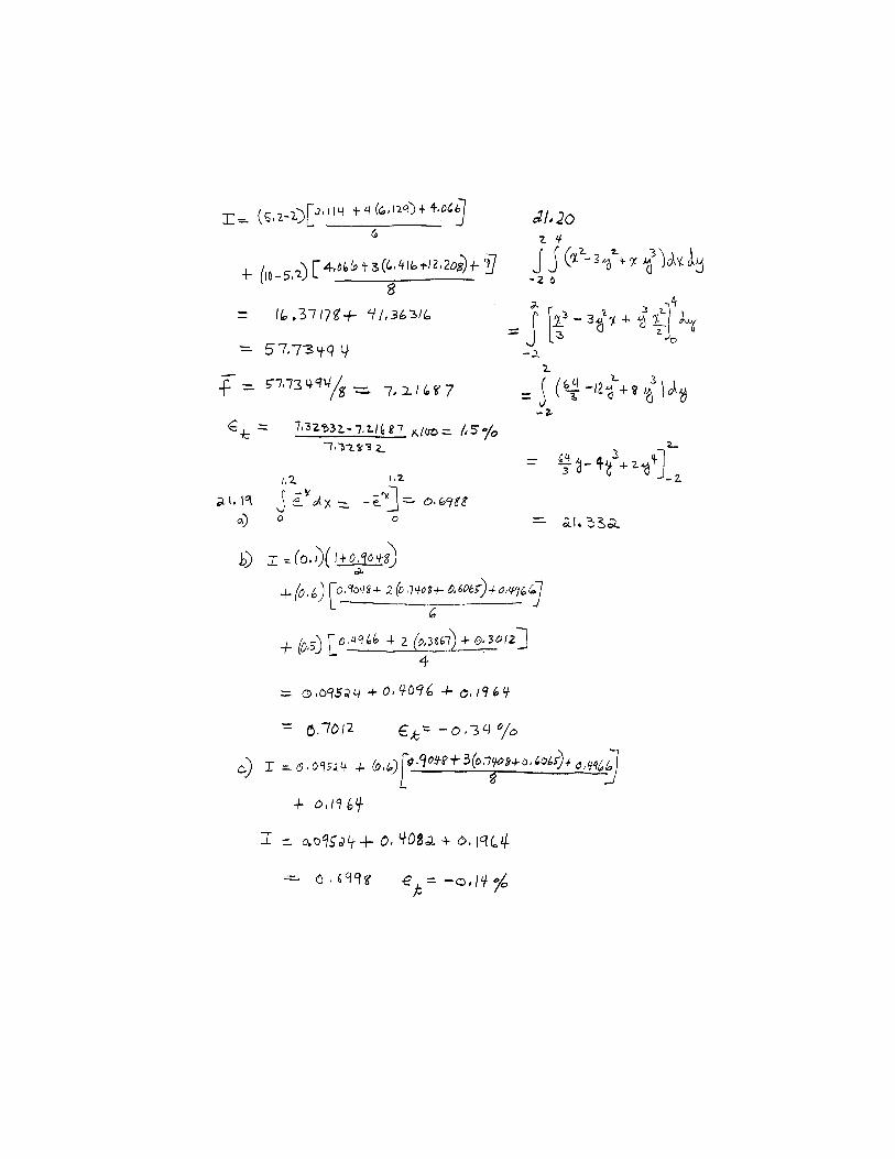

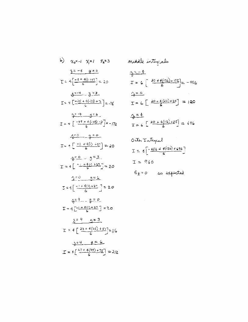

21.22 Here is a VBA code to implement the multi-segment trapezoidal rule for equally-spacedsegments:
Option Explicit
Sub TestTrapm()
Dim n As Integer, i As Integer, ind As IntegerDim label As StringDim a As Single, b As Single, h As SingleDim x(100) As Single, f(100) As Single
'Enter data and integration parametersind = InputBox("Functional (1) or Tabulated (2) data?")a = InputBox("Lower bound = ")b = InputBox("Upper bound = ")n = InputBox("Number of segments = ")h = (b - a) / nIf ind = 1 Then 'generate data from function x(0) = a f(0) = fx(a) For i = 1 To n x(i) = x(i - 1) + h f(i) = fx(x(i)) Next iElse 'user input table of data x(0) = a label = "f(" & x(0) & ") = " f(i) = Val(InputBox(label)) For i = 1 To n x(i) = x(i - 1) + h label = "f(" & x(i) & ") = " f(i) = InputBox(label) Next iEnd If
'invoke function to determine and display integralMsgBox "The integral is " & Trapm(h, n, f())
End Sub
Function Trapm(h, n, f)Dim i As IntegerDim sum As Singlesum = f(0)For i = 1 To n - 1 sum = sum + 2 * f(i)Next isum = sum + f(n)Trapm = h * sum / 2End Function
Function fx(x)fx = 0.2 + 25 * x - 200 * x ^ 2 + 675 * x ^ 3 - 900 * x ^ 4 + 400 * x ^ 5End Function
21.23 Here is a VBA code to implement the multi-segment Simpson’s 1/3 rule algorithm fromFig. 21.13c:
Option Explicit
Sub TestSimpm()
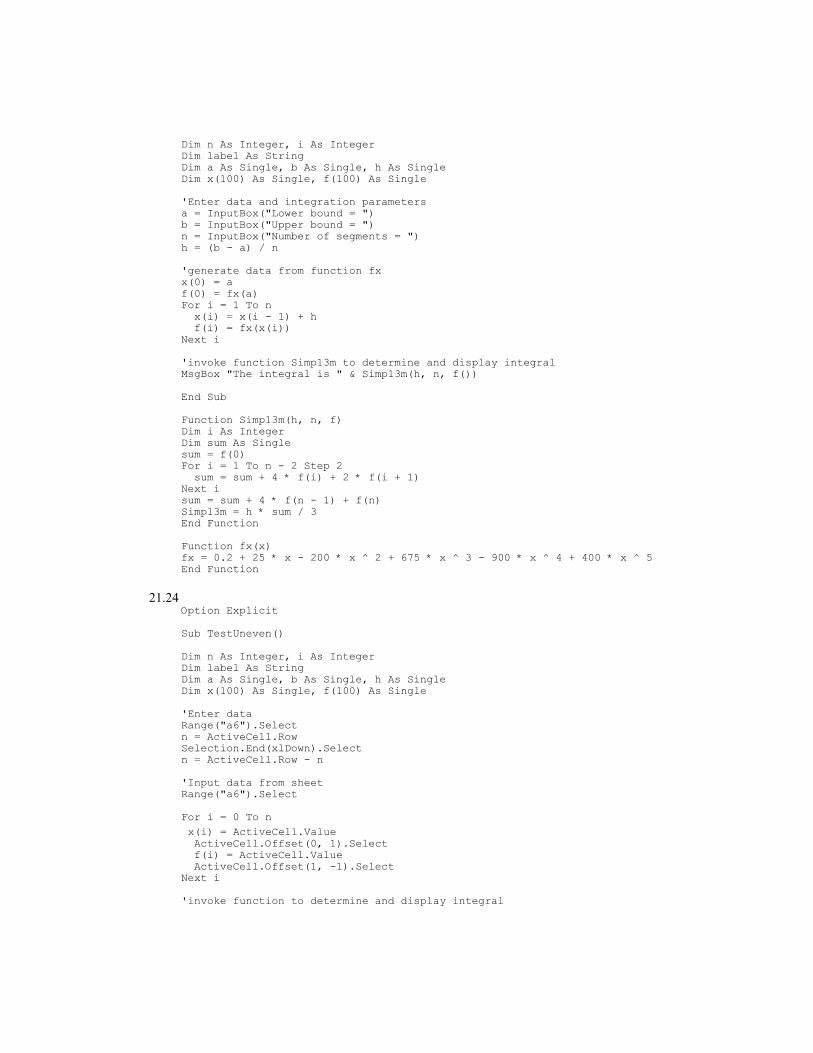
Dim n As Integer, i As IntegerDim label As StringDim a As Single, b As Single, h As SingleDim x(100) As Single, f(100) As Single
'Enter data and integration parametersa = InputBox("Lower bound = ")b = InputBox("Upper bound = ")n = InputBox("Number of segments = ")h = (b - a) / n
'generate data from function fxx(0) = af(0) = fx(a)For i = 1 To n x(i) = x(i - 1) + h f(i) = fx(x(i))Next i
'invoke function Simp13m to determine and display integralMsgBox "The integral is " & Simp13m(h, n, f())
End Sub
Function Simp13m(h, n, f)Dim i As IntegerDim sum As Singlesum = f(0)For i = 1 To n - 2 Step 2 sum = sum + 4 * f(i) + 2 * f(i + 1)Next isum = sum + 4 * f(n - 1) + f(n)Simp13m = h * sum / 3End Function
Function fx(x)fx = 0.2 + 25 * x - 200 * x ^ 2 + 675 * x ^ 3 - 900 * x ^ 4 + 400 * x ^ 5End Function
21.24Option Explicit
Sub TestUneven()
Dim n As Integer, i As IntegerDim label As StringDim a As Single, b As Single, h As SingleDim x(100) As Single, f(100) As Single
'Enter dataRange("a6").Selectn = ActiveCell.RowSelection.End(xlDown).Selectn = ActiveCell.Row - n
'Input data from sheetRange("a6").Select
For i = 0 To n
x(i) = ActiveCell.Value ActiveCell.Offset(0, 1).Select f(i) = ActiveCell.Value ActiveCell.Offset(1, -1).SelectNext i
'invoke function to determine and display integral

MsgBox "The integral is " & Uneven(n, x(), f())
End Sub
Function Uneven(n, x, f)Dim k As Integer, j As IntegerDim h As Single, sum As Single, hf As Singleh = x(1) - x(0)k = 1sum = 0#For j = 1 To n hf = x(j + 1) - x(j)
If Abs(h - hf) < 0.000001 Then If k = 3 Then sum = sum + Simp13(h, f(j - 3), f(j - 2), f(j - 1)) k = k - 1 Else k = k + 1 End If Else If k = 1 Then sum = sum + Trap(h, f(j - 1), f(j)) Else If k = 2 Then sum = sum + Simp13(h, f(j - 2), f(j - 1), f(j)) Else sum = sum + Simp38(h, f(j - 3), f(j - 2), f(j - 1), f(j)) End If k = 1 End If End If h = hfNext jUneven = sumEnd Function
Function Trap(h, f0, f1)Trap = h * (f0 + f1) / 2End Function
Function Simp13(h, f0, f1, f2)Simp13 = 2 * h * (f0 + 4 * f1 + f2) / 6End Function
Function Simp38(h, f0, f1, f2, f3)Simp38 = 3 * h * (f0 + 3 * (f1 + f2) + f3) / 8End Function
Function fx(x)fx = 0.2 + 25 * x - 200 * x ^ 2 + 675 * x ^ 3 - 900 * x ^ 4 + 400 * x ^ 5End Function
21.25 (a)
]2
)()(2)()[(
1
1
n
xfxfxfabM
n
i nio ∑ −
=++
−=
ft-lb 110.825
)11(2
15.22)1915.166.1335.114.975.74.635.56.415.4(24)011(
=
+++++++++++−=M
(b) The 1/3 rule can only be applied to the first 10 panels. The trapezoidal rule can beapplied to the 11th

ft-lb 825.1102
15.2219)1112(
])10(3
19)6.134.94.66.4(2)15.1635.1175.735.515.4(44)[010(
=+
−+
++++++++++−=M
(c) The 3/8 rule can only be applied to the first 9 panels and the 1/3 rule applied to the last2:
ft-lb 55.110]6
15.22)19(415.16)[911(]
8
15.16)6.1335.11(34.9)[69(
]8
4.9)75.74.6(335.5)[36(]
8
35.5)6.415.4(34)[03(
=++
−++++
−+
+++−+
+++−=M
This result is exact because we’re integrating a quadratic. The results of (a) and (b) are notexact because they include trapezoidal rule evaluations.
21.26Divide the curve into sections according to dV changes and use appropriate rules.
583.2421
5.224)2
207242(1
75.930)242)312(3)326(3326(8
3
33.675)326)333(4368(3
1
591)2
368420(5.1
4321
4
3
2
1
=+++=
=+
=
=+++=
=++=
=+
=
IIIIW
I
I
I
I
Therefore, the work done is 2420 kJ.
21.27 (a) The trapezoidal rule yields 60.425.
(b) A parabola can be fit to the data to give
y = -0.11829x2 + 1.40701x + 3.36800
R2 = 0.60901
4
5
6
7
8
9
10
0 2 4 6 8 10 12
The parabola can be integrated and evaluated from 1 to 10 to give 60.565.

(c) A cubic can be fit to the data to give
y = -0.01672x3 + 0.16015x2 + 0.10764x + 4.81478
R2 = 0.67487
4
5
6
7
8
9
10
0 2 4 6 8 10 12
The cubic can be integrated and evaluated from 1 to 10 to give 60.195.
Although it’s not asked in the problem statement, the algorithm from Fig. 21.15b can alsobe applied (see Solution to Prob. 20.24 for code) to yield 60.258.
21.28 (a) The following 2 equations must hold:
raQeaf =)( (1)
rbQebf =)( (2)
Take the natural log of Eq. 1 and solve for
raafQ −= )(lnln (3)
or
raeafQ −= )( (4)
Substituting (3) into the natural log of Eq. 2 gives
rbraafbf +−= )(ln)(ln (5)
and solve for
( )ba
bfafr
−=
)(/)(ln (6)
These results can be verified for the case where Q = 3 and r = −0.5. If a = 2 and b = 4, f(a)= 1.1036 and f(b) = 0.406. Substituting these values into Eqs. 6 and 4 gives
5.042
)406.0/0136.1ln(−=
−=r
31036.1 2)5.0()2)(5.0()1036.1ln( === −−−− eeQ

(b)
( )rarbb
a
rx eer
QdxQeI −== ∫
Substituting Eq. 4
( ) ( )1)()( )( −=−= −
−abrrarb
ra
er
afee
r
eafI
Substituting Eq. 6
( )
( )
−
−
=−
− 1)(/)(ln
)( )()(/)(ln
abba
bfaf
e
ba
bfaf
afI
Simplifying
( )( ))(/)(ln
)()()(
afbf
afbfabI
−−=
This result can be verified for the case where Q = 3 and r = −0.5. If a = 2 and b = 4, f(a) =1.1036 and f(b) = 0.406. Substituting these values into the integral equation gives
( )( )
9353.11036.1/406.0ln
1036.1406.0)24(=
−−=I
which matches the analytical integral
( ) 9353.15.0
3 )2(5.0)4(5.0 =−−
== −− eeI


22.11Option Explicit
Sub RhombTest()Dim maxit As IntegerDim a As Single, b As Single, es As Singlea = 0b = 0.8maxit = 3es = 0.001MsgBox Rhomberg(a, b, maxit, es)End Sub
Function Rhomberg(a, b, maxit, es)Dim n As Integer, j As Integer, k As Integer, iter As IntegerDim i(10, 10) As Single, ea As Singlen = 1i(1, 1) = TrapEq(n, a, b)iter = 0Do iter = iter + 1 n = 2 ^ iter i(iter + 1, 1) = TrapEq(n, a, b) For k = 2 To iter + 1 j = 2 + iter - k i(j, k) = (4 ^ (k - 1) * i(j + 1, k - 1) - i(j, k - 1)) / (4 ^ (k - 1)- 1) Next k ea = Abs((i(1, iter + 1) - i(1, iter)) / i(1, iter + 1)) * 100 If (iter >= maxit Or ea <= es) Then Exit DoLoopRhomberg = i(1, iter + 1)End Function
Function TrapEq(n, a, b)Dim i As IntegerDim h As Single, x As Single, sum As Singleh = (b - a) / nx = asum = f(x)For i = 1 To n - 1 x = x + h sum = sum + 2 * f(x)Next isum = sum + f(b)

TrapEq = (b - a) * sum / (2 * n)End Function
Function f(x)f = 0.2 + 25 * x - 200 * x ^ 2 + 675 * x ^ 3 - 900 * x ^ 4 + 400 * x ^ 5End Function
22.12Option Explicit
Sub GaussQuadTest()Dim i As Integer, j As Integer, k As IntegerDim a As Single, b As Single, a0 As Single, a1 As Single, sum As SingleDim c(11) As Single, x(11) As Single, j0(5) As Single, j1(5) As Single
'set constantsc(1) = 1#: c(2) = 0.888888889: c(3) = 0.555555556: c(4) = 0.652145155c(5) = 0.347854845: c(6) = 0.568888889: c(7) = 0.478628671: c(8) =0.236926885c(9) = 0.467913935: c(10) = 0.360761573: c(11) = 0.171324492x(1) = 0.577350269: x(2) = 0: x(3) = 0.774596669: x(4) = 0.339981044x(5) = 0.861136312: x(6) = 0: x(7) = 0.53846931: x(8) = 0.906179846x(9) = 0.238619186: x(10) = 0.661209386: x(11) = 0.932469514j0(1) = 1: j0(2) = 3: j0(3) = 4: j0(4) = 7: j0(5) = 9j1(1) = 1: j1(2) = 3: j1(3) = 5: j1(4) = 8: j1(5) = 11
a = 0b = 0.8Sheets("Sheet1").SelectRange("a1").SelectFor i = 1 To 5 ActiveCell.Value = GaussQuad(i, a, b, c(), x(), j0(), j1()) ActiveCell.Offset(1, 0).SelectNext iEnd Sub
Function GaussQuad(n, a, b, c, x, j0, j1)
Dim k As Integer, j As IntegerDim a0 As Single, a1 As SingleDim sum As Single
a0 = (b + a) / 2a1 = (b - a) / 2sum = 0If Int(n / 2) - n / 2# = 0 Then k = (n - 1) * 2 sum = sum + c(k) * a1 * f(fc(x(k), a0, a1))End IfFor j = j0(n) To j1(n) sum = sum + c(j) * a1 * f(fc(-x(j), a0, a1)) sum = sum + c(j) * a1 * f(fc(x(j), a0, a1))Next jGaussQuad = sumEnd Function
Function fc(xd, a0, a1)fc = a0 + a1 * xdEnd Function
Function f(x)f = 0.2 + 25 * x - 200 * x ^ 2 + 675 * x ^ 3 - 900 * x ^ 4 + 400 * x ^ 5End Function

22.13
See solutions for Probs. 22.1, 22.2 and 22.3 for answers
22.14
See solutions for Probs. 22.4, 22.5 and 22.6 for answers
22.15Option Explicit
Sub TestMidPoint()
Dim i As Integer, j As Integer, d As IntegerDim a As Single, b As Single, h As Single, x As SingleDim sum As Single, ea As Single, es As SingleDim integral As Single, integralold As Single
a = -0.5b = 0es = 0.01
Range("a5").SelectSheets("Sheet1").Range("a5:d25").ClearContentsDo integralold = integral d = 3 ^ i h = (b - a) / d x = a - h / 2 sum = 0 ActiveCell.Value = d ActiveCell.Offset(0, 1).Select ActiveCell.Value = h ActiveCell.Offset(0, 1).Select For j = 1 To d x = x + h sum = sum + f(x) Next j integral = sum * h i = i + 1 ActiveCell.Value = integral ActiveCell.Offset(0, 1).Select ea = Abs((integral - integralold) / integral) * 100 ActiveCell.Value = ea ActiveCell.Offset(1, -3).Select If ea < es Then Exit DoLoop
End Sub
Function f(x)f = 1 / x ^ 2 * Exp(-1 / (2 * x ^ 2))End Function


23.10Option Explicit
Sub RhombTest()Dim maxit As IntegerDim a As Single, b As Single, es As SingleDim x As Singlex = 0.5maxit = 3es = 0.001MsgBox RhomDiff(x, maxit, es)End Sub
Function RhomDiff(x, maxit, es)Dim n As Integer, j As Integer, k As Integer, iter As IntegerDim i(10, 10) As Single, ea As Single, del As Single, a As Single, b As Singlen = 1i(1, 1) = DyDx(x, n)iter = 0
Do iter = iter + 1 n = 2 ^ iter i(iter + 1, 1) = DyDx(x, n) For k = 2 To iter + 1 j = 2 + iter - k i(j, k) = (4 ^ (k - 1) * i(j + 1, k - 1) - i(j, k - 1)) / (4 ^ (k - 1) - 1) Next k ea = Abs((i(1, iter + 1) - i(1, iter)) / i(1, iter + 1)) * 100 If (iter >= maxit Or ea <= es) Then Exit DoLoopRhomDiff = i(1, iter + 1)End Function
Function DyDx(x, n)Dim a As Single, b As Singlea = x - x / nb = x + x / nDyDx = (f(b) - f(a)) / (b - a)End Function
Function f(x)f = -0.1 * x ^ 4 - 0.15 * x ^ 3 - 0.5 * x ^ 2 - 0.25 * x + 1.2End Function
23.11 The following program implements Eq. 23.9.
Option Explicit
Sub TestDerivUnequal()
Dim n As Integer, i As IntegerDim x(100) As Single, y(100) As Single, dy(100) As Single
Range("a5").Selectn = ActiveCell.RowSelection.End(xlDown).Selectn = ActiveCell.Row - nRange("a5").SelectFor i = 0 To n x(i) = ActiveCell.Value ActiveCell.Offset(0, 1).Select y(i) = ActiveCell.Value

ActiveCell.Offset(1, -1).SelectNext i
For i = 0 To n dy(i) = DerivUnequal(x(), y(), n, x(i))Next i Range("c5").SelectFor i = 0 To n ActiveCell.Value = dy(i) ActiveCell.Offset(1, 0).SelectNext iEnd Sub
Function DerivUnequal(x, y, n, xx)
Dim ii As Integer
If xx < x(0) Or xx > x(n) Then DerivUnequal = "out of range"Else If xx < x(1) Then DerivUnequal = DyDx(xx, x(0), x(1), x(2), y(0), y(1), y(2)) ElseIf xx > x(n - 1) Then DerivUnequal = DyDx(xx, x(n - 2), x(n - 1), x(n), y(n - 2), y(n - 1),y(n)) Else For ii = 1 To n - 2 If xx >= x(ii) And xx <= x(ii + 1) Then If xx - x(ii - 1) < x(ii) - xx Then 'If the unknown is closer to the lower end of the range, 'x(ii) will be chosen as the middle point DerivUnequal = DyDx(xx, x(ii - 1), x(ii), x(ii + 1), y(ii - 1),y(ii), y(ii + 1)) Else 'Otherwise, if the unknown is closer to the upper end, 'x(ii+1) will be chosen as the middle point DerivUnequal = DyDx(xx, x(ii), x(ii + 1), x(ii + 2), y(ii), y(ii+ 1), y(ii + 2)) End If Exit For End If Next ii End IfEnd If
End Function
Function DyDx(x, x0, x1, x2, y0, y1, y2)DyDx = y0 * (2 * x - x1 - x2) / (x0 - x1) / (x0 - x2) _ + y1 * (2 * x - x0 - x2) / (x1 - x0) / (x1 - x2) _ + y2 * (2 * x - x0 - x1) / (x2 - x0) / (x2 - x1)End Function
The result is

An even more elegant approach is to put cubic splines through the data (recall Sec. 20.2and the solution for Prob. 20.10) to evaluate the derivatives.
23.12(a) Create the following M function:
function y=f(x)y=9.8*68.1/12.5*(1-exp(-12.5/68.1*x));
Then implement the following MATLAB session:
>> Q=quad('f',0,10)
Q = 289.4351
(b)
( )∫ −−=t
tmc dtec
gmtd
0
)/( 1)(
ttmc
ec
mt
c
gmtd
0
)/()(
+= −
4351.2895.12
1.680
5.12
1.6810
5.12
)1.68(8.9)(
10
0
10)1.68/5.12( =
−−+= −
etd
(c) Create the following M function:
>> function y=f(x)

>> y=9.8*68.1/12.5*(1-exp(-12.5/68.1*x));
Then implement the following MATLAB session:
>> x=[9.99 10.01]>> y=f(x)>> d=diff(y)./diff(x)
d = 1.5634
(d)
( )tmcedt
d
c
gmta )/(1)( −−=
tmcgeta )/()( −=
56337.18.9)( 10)1.68/5.12( −== −eta
23.13 (a) Create the following M function:
function y=fn(x)y=1/sqrt(2*pi)*exp(-(x.^2)/2);
Then implement the following MATLAB session:
>> x=-2:.1:2;>> y=fn(x);>> Q=quad('fn',-1,1)
Q = 0.6827
>> Q=quad('fn',-2,2)
Q = 0.9545
Thus, about 68.3% of the area under the curve falls between –1 and 1 and about 95.45%falls between –2 and 2.
(b)
>> x=-2:.1:2>> y=fn(x)>> d=diff(y)./diff(x)>> x=-1.95:.1:1.95>> d2=diff(d)./diff(x)>> x=-1.9:.1:1.9>> plot(x,d2,'o')

Thus, inflection points (d2y/dx2 = 0) occur at –1 and 1.
23.14 (a) Create the following M function:
function y=fn(x)y=1/sqrt(2*pi)*exp(-(x.^2)/2);
Then implement the following MATLAB session:
>> x=-2:.5:2;>> y=fn(x);>> Q=quad('fn',-1,1)
Q = 0.6827
>> Q=quad('fn',-2,2)
Q = 0.9545
Thus, about 68.3% of the area under the curve falls between –1 and 1 and about 95.45%falls between –2 and 2.
(b)
>> d=diff(y)./diff(x);>> x=-1.75:.5:1.75;>> d2=diff(d)./diff(x);>> x=-1.5:.5:1.5;>> plot(x,d2,'o')

Thus, inflection points (d2y/dx2 = 0) occur at –1 and 1.
23.15Program IntegrateUse imslImplicit NoneInteger::irule=1Real::a=-1.,b=1,errabs=0.0,errrel=0.001Real::errest,res,fExternal fCall QDAG(f,a,b,errabs,errrel,irule,res,errest)Print '('' Computed = '',F8.4)',resPrint '('' Error estimate ='',1PE10.3)',errestEnd Program
Function f(x)Implicit NoneReal:: x , fReal::piParameter(pi=3.1415927)f=1/sqrt(2*pi)*exp(-x**2/2)End Function
Answers:
x = -1 to 1: Computed = 0.6827 Error estimate = 4.069E-06x = -2 to 2: Computed = 0.9545 Error estimate = 7.975E-06x = -3 to 3: Computed = 0.9973 Error estimate = 5.944E-06
23.16 MATLAB Script:
% Prob2316 Integration programa=0;b=pi/2;integral=quad('ff',a,b)end

function y=ff(x);y=sin(sin(x));
>> prob2316
integral = 0.8932
23.17 MATLAB Script:
%Numerical Integration of sin(t)/t = function sint(t)%Limits: a=0, b=2pi%Using the "quad" and "quadl" function for numerical integration%Plot of functiont=0.01:0.01:2*pi;y=ff2(t);plot(t,y); grid%Integrationformat longa=0.01;b=2*pi;Iquad=quad('ff2',a,b)Iquadl=quadl('ff2',a,b)
function y=ff2(t);y=sin(t)./t;
MATLAB execution:
>> prob2317
Iquad = 1.40815164305082
Iquadl = 1.40815163168846

23.18%Centered Finite Difference First & Second Derivatives of Order O(dx^2)%Using diff(y)
dx=0.5;y=[1.4 2.1 3.3 4.7 7.1 6.4 8.8 7.2 8.9 10.7 9.8];dyf=diff(y);
% First Derivative Centered FD using diffn=length(y);for i=1:n-2
dydxc(i)=(dyf(i+1)+dyf(i))/(2*dx);end
%Second Derivative Centered FD using diffdy2dx2c=diff(dyf)/(dx*dx);
fprintf('first derivative \n'); fprintf('%f\n', dydxc)fprintf('second derivative \n'); fprintf('%f\n', dy2dx2c)
first derivative 1.9000002.6000003.8000001.7000001.7000000.8000000.1000003.5000000.900000second derivative 2.0000000.8000004.000000-12.40000012.400000-16.00000013.2000000.400000-10.800000

23.19% Finite Difference Approximation of slope% For f(x)=exp(-x)-x% f'(x)=-exp(-x)-1% Centered diff. df/dx=(f(i+1)-f(i-1))/2dx + O(dx^2)% Fwd. diff. df/dx=(-f(i+2)+4f(i+1)-3f(i))/2dx + O(dx^2)% Bkwd. diff. df/dx=(3f(i)-4f(i-1)+f(i-2))/2dx + O(dx^2)
x=2;fx=exp(-x)-x;dfdx2=-exp(-x)-1;
%approximationdx=0.5:-0.01:.01;for i=1:length(dx)
%x-values at i+-dx and +-2dxxp(i)=x+dx(i);x2p(i)=x+2*dx(i);xn(i)=x-dx(i);x2n(i)=x-2*dx(i);
%f(x)-values at i+-dx and +-2dxfp(i)=exp(-xp(i))-xp(i);f2p(i)=exp(-x2p(i))-x2p(i);fn(i)=exp(-xn(i))-xn(i);f2n(i)=exp(-x2n(i))-x2n(i);
%Finite Diff. ApproximationsCdfdx(i)=(fp(i)-fn(i))/(2*dx(i));
Fdfdx(i)=(-f2p(i)+4*fp(i)-3*fx)/(2*dx(i));Bdfdx(i)=(3*fx-4*fn(i)+f2n(i))/(2*dx(i));
enddx0=0;plot(dx,Fdfdx,'--',dx,Bdfdx,'-.',dx,Cdfdx,'-',dx0,dfdx2,'*')
gridtitle('Forward, Backward, and Centered Finite Difference approximation - 2nd
Order Correct')xlabel('Delta x')ylabel('df/dx')gtext('Centered'); gtext('Forward'); gtext('Backward')

0 0.05 0.1 0.15 0.2 0.25 0.3 0.35 0.4 0.45 0.5-1.145
-1.14
-1.135
-1.13
-1.125
-1.12
-1.115
-1.11Forward, B ac kward, and Centered F inite Difference approx im ation - 2nd Order Correc t
Delta x
df/d
x
Centered
Forward
B ac kward

23.20
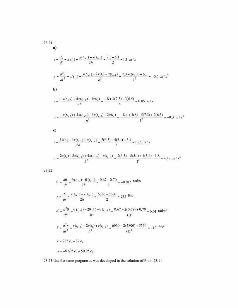
23.21
a)
2
22
11
2
2
11
/6.01
1.5)5.6(23.7)()(2)()(
/1.12
1.53.7
2
)()()(
smh
txtxtxtx
dt
xda
smh
txtxtx
dt
dxv
iiii
iii
−=+−
=+−
=′′==
=−
=−
=′==
−+
−+
b)
2
22123
12
/3.01
)3.6(2)3.7(5)8(44.8)(2)(5)(4)(
/85.02
)5.6(3)3.7(48
2
)(3)(4)(
smh
txtxtxtxa
smh
txtxtxv
iiii
iii
−=+−+−
=+−+−
=
=−+−
=−+−
=
+++
++
c)
2
22321
21
/7.01
8.1)4.3(4)1.5(5)5.6(2)()(4)(5)(2
/25.12
4.3)1.5(4)5.6(3
2
)()(4)(3
smh
txtxtxtxa
smh
txtxtxv
iiii
iii
−=−+−
=−+−
=
=+−
=+−
=
−−−
−−
23.22
015.02
70.067.0
2
)()( 11 −=−
=−
== −+
h
tt
dt
d ii θθθθ rad/s
2352
55606030
2
)()( 11 =−
=−
== −+
h
trtr
dt
drr ii ft/s
01.0)1(
70.0)68.0(267.0)()(2)(22
11
2
2
=+−
=+−
== −+
h
ttt
dt
d iii θθθθθ rad/s2
10)1(
5560)5800(26030)()(2)(22
11
2
2
−=+−
=+−
== −+
h
trtrtr
dt
rdr iii ft/s2
θeev r
87235 −=
θeea r
95.50695.8 +−=
23.23 Use the same program as was developed in the solution of Prob. 23.11

23.24


24.9


24.10
Time After Injection (sec) Semilog Dye Concentration Constant Product
9 0.11 1 0.11
9.5 0.14 2 0.28
10 0.18 2 0.36
10.5 0.25 2 0.5
11 0.4 2 0.8
11.5 0.7 2 1.4
12 1.4 2 2.8
12.5 2.4 2 4.8
13 4 2 8
13.5 5.5 2 11
14 6.85 2 13.7
14.5 8 2 16

15 9 2 18
15.5 9.35 2 18.7
16 9.2 2 18.4
16.5 8.7 2 17.4
17 7.95 2 15.9
17.5 7 2 14
18 5.95 2 11.9
18.5 4.85 2 9.7
19 4.1 2 8.2
19.5 3.5 2 7
20 3 2 6
20.5 2.55 2 5.1
21 2.2 2 4.4
21.5 1.8 2 3.6
22 1.5 2 3
22.5 1.3 2 2.6
23 1.1 2 2.2
23.5 0.9 2 1.8
24 0.8 2 1.6
24.5 0.64 2 1.28
25 0.55 2 1.1
25.5 0.47 2 0.94
26 0.4 2 0.8
26.5 0.34 2 0.68
27 0.29 2 0.58
27.5 0.24 2 0.48
28 0.2 2 0.4
28.5 0.16 2 0.32
29 0.14 2 0.28
29.5 0.125 2 0.25
30 0.1 1 0.1
Sum of Products = 236.46
Trapezoidal Approximation = 59.115
Cardiac Output = [56 mg/59.115 mg*sec/L]*60 = 5.68 L/min

24.11 The following Excel Solver application can be used to estimate: k = 0.09915 and A=6.98301.
24.12 The following Excel spreadsheet is set up to use (left) a combination of the trapezoidal andSimpsons rules and (right) just the trapezoidal rule:

24.13
The extremes for both cases are at 16 and 92


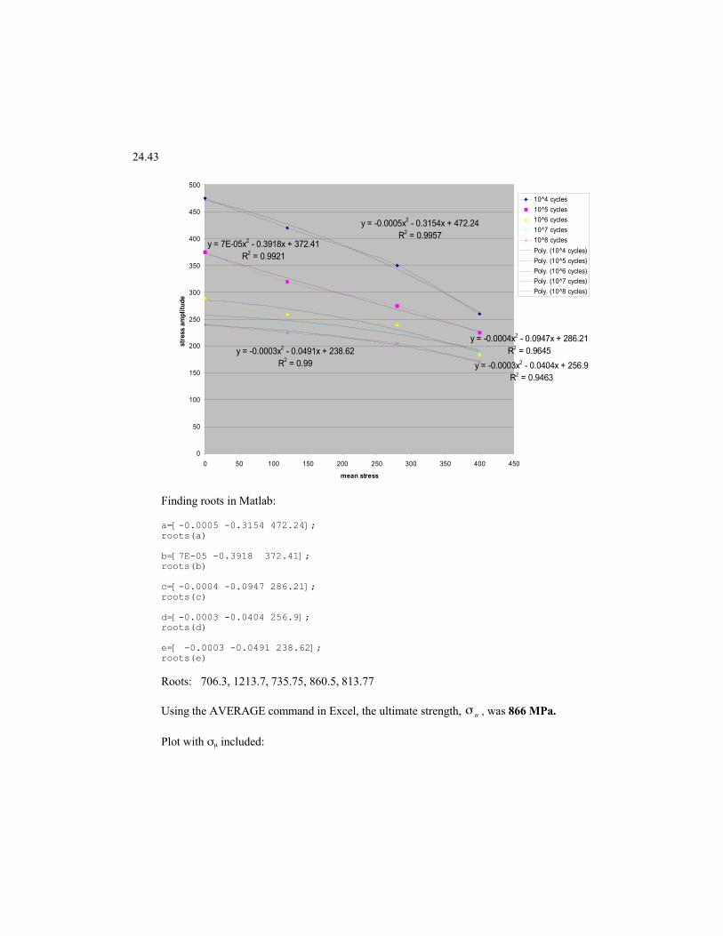
24.43
y = -0.0005x2 - 0.3154x + 472.24
R2 = 0.9957
y = 7E-05x2 - 0.3918x + 372.41
R2 = 0.9921
y = -0.0004x2 - 0.0947x + 286.21
R2 = 0.9645
y = -0.0003x2 - 0.0404x + 256.9
R2 = 0.9463
y = -0.0003x2 - 0.0491x + 238.62
R2 = 0.99
0
50
100
150
200
250
300
350
400
450
500
0 50 100 150 200 250 300 350 400 450
mean stress
str
ess a
mp
litu
de
10^4 cycles
10^5 cycles
10^6 cycles
10^7 cycles
10^8 cycles
Poly. (10^4 cycles)
Poly. (10^5 cycles)
Poly. (10^6 cycles)
Poly. (10^7 cycles)
Poly. (10^8 cycles)
Finding roots in Matlab:
a=[-0.0005 -0.3154 472.24];roots(a) b=[7E-05 -0.3918 372.41];roots(b) c=[-0.0004 -0.0947 286.21];roots(c)
d=[-0.0003 -0.0404 256.9];roots(d)
e=[ -0.0003 -0.0491 238.62];roots(e)
Roots: 706.3, 1213.7, 735.75, 860.5, 813.77
Using the AVERAGE command in Excel, the ultimate strength, uσ , was 866 MPa.
Plot with σµ included:

y = -0.0005x2 - 0.3307x + 472.76
R2 = 0.9992
10^4 cycles
y = 7E-05x2 - 0.3894x + 372.32
R2 = 0.9988
10^5 cycles
y = -0.0004x2 - 0.0746x + 285.51
R2 = 0.996
10^6 cycles
y = -0.0003x2 - 0.0389x + 256.84
R2 = 0.9969
10^7 cycles
y = -0.0003x2 - 0.0474x + 238.56
R2 = 0.9993
10^8 cycles
-100
0
100
200
300
400
500
600
0 200 400 600 800 1000 1200
mean stress
str
ess a
mp
litu
de
10^4 cycles
10^5 cycles
10^6 cycles
10^7 cycles
10^8 cycles
Poly. (10^4 cycles)
Poly. (10^5 cycles)
Poly. (10^6 cycles)
Poly. (10^7 cycles)
Poly. (10^8 cycles)
It can be seen from the higher R2 values that the polynomial fit including the ultimate
stress, uσ , is more accurate than the fit without including uσ .
24.44This problem was solved using Excel.
0
0.01
0.02
0.03
0.04
0.05
0.06
0.07
0 2 4 6 8 10 12
t i me , mi n
Thefollowing values were calculated beginning with the ninth data point of the series.
Mean = 0.045305
Standard Deviation = 0.003716

24.45 This problem was solved using Excel.
a) Find the equation for velocity using Excel.
y = -0.0499x2 + 0.0271x + 2.9699
R2 = 0.9976
-0.5
0
0.5
1
1.5
2
2.5
3
3.5
0 1 2 3 4 5 6 7 8 9
ra d i us , r
∫=R
drurQ
0
2π
Integrate according to the equation above, using R = 8 in.
Q = 2.12 ft3/s
b)
8*3
0*8)4.1*636.2*478.2*2(2)67.0*778.1*561.2*392.2*1(43*0)8(*2
3
)()(2)(4)(
)(
2
6,4,2
1
5,3,1
0
++++++++≅
+++
−≅
∑∑−
=
−
=
πI
n
xfxfxfxf
abI
n
n
j
j
n
i
i
I≅ 2.097 ft3/s
c) % error = %10.1100*12.2
12.2097.2=
−
24.46 a) Find the equation for velocity using Excel.

y = -0.1914x2 + 0.3666x + 4.754
R2 = 0.9835
0
1
2
3
4
5
6
0 1 2 3 4 5 6rad ius , r
∫=2
1
2
r
r
drurQ π
To find the volume flow rate in the region around the plug, integrate according to theequation above, using r1=1 in. and r2 = 6 in.
Q1 = 2.073 ft3/s
To find the volume flow rate of the plug, use cc AuQ =2
Q2 = 0.1091 ft3/s
Q = Q1 + Q2 = 2.182 ft3/s
Q = 2.182 ft3/s
b) Integral for the outer region:
5*3
6*0)69.1*501.4*3(2)42.3*462.4*2(45*1)5(*2
3
)()(2)(4)(
)(
2
6,4,2
1
5,3,1
0
+++++≅
+++
−≅
∑∑−
=
−
=
πI
n
xfxfxfxf
abI
n
n
j
j
n
i
i
I≅ 2.002 ft3/s

Inner region Q2 = 0.1091 ft3/s remains the same.
Therefore, the volume flow rate Q = 2.111 ft3/s.
c) % error = %36.3111.2
182.2111.2=
−
24.47 The following Excel worksheet solves the problem. Note that the derivative is calculatedwith a centered difference,
K
VV
dT
dV KK
100
350450 −=
24.48 A single application of the trapezoidal rule yields:
1.1332
11.12.12)222( =
+−=I
A 2-segment trapezoidal rule gives
95.864
11.1)04.2(22.12)222( =
++−=I
A 4-segment trapezoidal rule gives
125.688
11.1)44.104.249.3(22.12)222( =
++++−=I
Because we do not know the true value, it it would seem impossible to estimate the error.However, we can try to fit different order polynomials to see if we can get a decent fit tothe data. This yields the surprising result that a 4th-order polynomial results in almost aperfect fit. For example, using the Excel trend line gives:

y = 3.88667E-04x4 - 2.33160E-02x
3 +
5.10851E-01x2 - 4.96288E+00x +
2.02627E+01
R2 = 1.00000E+00
0
4
8
12
0 6 12 18 24
This can be integrated analytically to give 61.20365. Note that the same result would resultfrom using Boole’s rule, Rhomberg integration or Gauss quadrature.1
Therefore, we can estimate the errors as
%47.117%10061.20365
1.13361.20365=×
−=I
%07.42%10061.20365
95.8661.20365=×
−=I
%31.11%10061.20365
125.6861.20365=×
−=I
The ratio of these is 117.47:42.07:11.31 = 10.4:3.7:1. Thus it approximates the quarteringof the error that we would expect according to Eq. 21.13.
24.49 (b) This problem can be solved in a number of ways. One approach is to set up Excel witha series of equally-spaced x values from 0 to 100. Then one of the formulas described inthis Part of the book can be used to numerically compute the derivative. For example, Iused x values with an interval of 1 and Eq. 23.9. The resulting plot of the function and itsderivative is
1 There might be a slight discrepancy due to roundoff.

0
0.2
0.4
0.6
0.8
1
0 20 40 60 80 100
0
0.01
0.02
0.03
(b) Inspection of this plot indicates that the maximum derivative occurs at about a diameterof 13.3.
(c) The function to be integrated looks like
f(x)/x
0
0.004
0.008
0.012
0 20 40 60 80 100
This can be integrated from 1 to a high number using any of the methods provided in thisbook. For example, the Trapezoidal rule can be used to integrate from 1 to 100, 1 to 200and 1 to 300 using h = 1. The results are:
h I100 0.073599883200 0.073632607300 0.073632609
Thus, the integral seems to be converging to a value of 0.073633. Sm can be computed as
6×0.073633 = 0.4418.

CHAPTER 28
28.1 The solution with the 2nd-order RK (Heun without corrector) can be laid out as
For the 4th-order RK, the solution is
A plot of both solutions along with the analytical result is displayed below:
0
25
50
0 20 40
Analytical
RK-4
RK-2
28.2 The mass-balance equations can be written as
dc
dtc c1
1 3014 0 04= − +. .
dc
dtc c2
1 20 2 0 2= −. .
dc
dtc c3
2 30 025 0 275= −. .
dc
dtc c c4
3 4 501125 0175 0 025= − +. . .
dc
dtc c c5
1 2 50 03 0 03 0 06= + −. . .
Selected solution results (Euler’s method) are displayed below, along with a plot of the results.
0
10
20
0 20 40 60 80
c1 c2 c3 c4 c5
Finally, MATLAB can be used to determine the eigenvalues and eigenvectors:

>> a=[.14 -.04 0 0 0;-.2 .2 0 0 0;0 -.025 .275 0 0;0 0 -.1125 .175 -.025;-.03-.03 0 0 .06]
a = 0.1400 -0.0400 0 0 0 -0.2000 0.2000 0 0 0 0 -0.0250 0.2750 0 0 0 0 -0.1125 0.1750 -0.0250 -0.0300 -0.0300 0 0 0.0600
>> [v,d]=eig(a)
v = 0 0 0 -0.1836 0.0826 0 0 0 -0.2954 -0.2567 0 0.6644 0 -0.0370 -0.6021 1.0000 -0.7474 0.2124 0.1890 0.7510 0 0 0.9772 0.9176 0.0256
d = 0.1750 0 0 0 0 0 0.2750 0 0 0 0 0 0.0600 0 0 0 0 0 0.0757 0 0 0 0 0 0.2643
28.3 Substituting the parameters into the differential equation gives
21.01.020 ccdt
dc−−=
The mid-point method can be applied with the result:
The results are approaching a value of 13.6351
Challenge question:
The steady state form (i.e., dc/dt = 0) of the equation is 22000 cc −−= , which can be solved
for 13.65097141 and -14.65097141. Thus, there is a negative root.
If we put in the initial y value as −14.650971 (or higher precision, the solution will stay at thenegative root. However, if we pick a value that is slightly higher (a per machine precision), it
will gravitate towards the positive root. For example if we use −14.65097

-20
-15
-10
-5
0
5
10
15
0 5 10
Conversely, if we use a slightly lower value, it will go unstable
-40
-30
-20
-10
0
0 5 10
28.4 The first steps of the solution are shown below along with a plot. Notice that the a value of theinflow concentration at the end of the interval (cin-end) is required to calculate the k2’s correctly.
0
50
0 50 100
28.5 The system is as depicted below:
qin = 10 kg/min qout = 10 kg/min
sin = 8 g/kg
s0 = 8 g/kg
M0 = 1000 kg
qevap = 0.5 kg/min
(a) The mass of water in the tank can be modeled with a simple mass balance
dM
dtq q q= − − = − − = −in out evap 10 10 05 0 5. .
With the initial condition that M = 1000 at t = 0, this equation can be integrated to yield,

M t= −1000 0 5.
Thus, the time to empty the tank (M = 0) can be calculated as t = 1000/0.5 = 2000 minutes.
(b) The concentration in the tank over this period can be computed in several ways. The simplestis to compute the mass of salt in the tank over time by solving the following differentialequation:
dm
dtq s q s= −in in out
where m = the mass of salt in the tank. The salt concentration in the tank, s, is the ratio of themass of salt to the mass of water
sm
M
m
t= =
−1000 05.
The first few steps of the solution of this ODE with Euler’s method is tabulated below. Inaddition, a graph of the entire solution is also displayed.
8
8.2
8.4
8.6
0 500 1000 1500 2000
Recognize that a singularity occurs at t = 2000, because the tank would be totally empty at thispoint.
28.6 A heat balance for the sphere can be written as
dH
dthA T Ta= −( )
The heat gain can be transformed into a volume loss by considering the latent heat of fusion.Thus,
dV
dt
hA
LT T
f
a= − −ρ
( ) (1)
where ρ = density ≅ 1 kg/m3 and Lf = latent heat of fusion ≅ 333 kJ/kg. The volume and area of asphere are computed by
V r A r=4
343 2π π =
(2)
These can be combined with (1) to yield,

dV
dt
hV
LT T
f
a=
−
43
4
2 3
ππ
ρ
/
( )
This equation can be integrated along with the initial condition,
V034
30 05= π ( . ) = 0.000524 m 3
to yield the resulting volume as a function of time.
V
t (s)0
0.0003
0.0006
0 100000 200000 300000
This result can be converted into diameter using (2)
d
t (s)
0
0.05
0.1
0 100000 200000 300000
28.7 The system for this problem is stiff. Thus, the use of a simple explicit Runge-Kutta schemewould involve using a very small time step in order to maintain a stable solution. A solverdesigned for stiff systems was used to generate the solution shown below. Two views of thesolution are given. The first is for the entire solution domain.
0
200
400
0 10 20 30
cb
ca
cc
In addition, we can enlarge the initial part of the solution to illustrate the fast transients thatoccur as the solution moves from its initial conditions to its dominant trajectories.

0
200
400
0 0.005 0.01 0.015 0.02
cb
cc
ca
28.8 Several methods could be used to obtain a solution for this problem (e.g., finite-difference,shooting method, finite-element). The finite-difference approach is straightforward:
DA A A
xkAi i i
i− +− +
− =1 1
2
20
∆
Substituting parameter values and collecting terms gives
− × + × + × − × =−−
− − −+1 10 2 10 4 10 1 10 0
61
6 6 2 61A x Ai i( )∆
Using a ∆x = 0.2 cm this equation can be written for all the interior nodes. The resulting linearsystem can be solved with an approach like the Gauss-Seidel method. The following table andgraph summarize the results.
0
0.05
0.1
0 1 2 3 4
28.9 The ODE to be solved is
a
tAP
a
b
dt
dP ωsin+−=
Substituting the parameters, it becomes
Ptdt
dP−= sin
The following Matlab script uses Euler’s method to solve the problem.
dt=0.05;max=5;n=max/dt+1;t=zeros(1,n);p=zeros(1,n);t(1)=0;p(1)=90;for i=1:n p(i+1)=p(i)+dydt(t(i),p(i))*dt; t(i+1)=t(i)+dt;end

plot(t,p)gridxlabel('Time-sec')ylabel('Pressure-mmHg')title('Pressure vs Time')zoom
function s=dydt(t,p);A=1;w=1;s=A*sin(w*t)-p;
0 1 2 3 4 5 6-10
0
10
20
30
40
50
60
70
80
90
Tim e-sec
Pre
ssur
e-m
mH
g
P ressure vs Tim e
28.10 Excel can be used to compute the basic results. As can be seen, the person died 1.13 hrs prior tobeing discovered. The non-self-starting Heun yielded the following time series of temperature:
60
80
100
120
0 1 2 3 4
28.11 The classical 4th order RK method yields

28.12 The classical 4th order RK method yields
28.13 (a) The first few steps of Euler’s method are shown in the following table
A plot of the entire simulation is shown below:
0
4
8
0 5 10 15 20
Notice that because the Euler method is lower order, the peaks are increasing, rather thanrepeating in a stable manner as time progresses. This result is reinforced when a state-space plotof the calculation is displayed.

0
3
6
0 5 10
(b) The first few steps of the Heun method is shown in the following table
A plot of the entire simulation is shown below:
0
4
8
0 5 10 15 20
Notice that in contrast to the Euler method, the peaks are stable manner as time progresses. Thisresult is also reinforced when a state-space plot of the calculation is displayed.
0
2
4
0 5
(c) The first few steps of the 4th-order RK method is shown in the following table
The results are quite close to those obtained with the Heun method in part (b). In fact, both thetime series and state-space plots are indistinguishable from each other.
28.14 Using the step size of 0.1, (a) and (b) both give unstable results. The 4th-order RK methodyields a stable solution. The first few values are shown in the following table. A plot of theresult for x is also shown below. Notice how after about t = 6, this solution diverges from thedouble precision version in Fig. 28.9.

-30
-20
-10
0
10
20
30
0 5 10 15 20
28.15 The second-order equation can be reexpressed as a pair of first-order equations,
dy
dzw
dw
dz
f
EIL z
=
= −2
2( )
We used Euler’s method with h = 1 to obtain the solution:
10
20
30
-0.5 0 0.5 1
z
y
28.16 The second-order equation can be reexpressed as a pair of first-order equations,
230/2
)(2)5(
200 zL
EIz
ze
dz
dww
dz
dy z
−+
==−
We used Euler’s method with h = 1 to obtain the solution:

z
y
10
20
30
-0.5 0 0.5 1
28.17 This problem was solved using the Excel spreadsheet in a fashion similar to the last example inSec. 28.1. We set up Euler’s method to solve the 3 ODEs using guesses for the diffusioncoefficients. Then we formed a column containing the squared residuals between ourpredictions and the measured values. Adjusting the diffusion coefficients with the Solver toolminimized the sum of the squares. At first, we assumed that the diffusion coefficients werezero. For this case the Solver did not converge on a credible answer. We then made guesses of
1×10⁷ for both. This magnitude was based on the fact that the volumes were of this order ofmagnitude. The resulting simulation did not fit the data very well, but was much better than
when we had guessed zero. When we used Solver, it converged on E12 = 9.22×10⁵ and E13 =
2.19×10⁶ which corresponded to a sum of the squares of residuals of 2.007. Some of the Eulercalculations are displayed below along with a plot of the fit.
0
50
100
0 5 10 15 20
It should be noted that we made up the “measurements” for this problem using the 4th-order RK
method with values for diffusive mixing of E12 = 1×10⁶ and E13 = 2×10⁶. We then used a randomnumber generator to add some error to this “data.”
28.18 The Heun method can be used to compute
The results can be plotted. In addition, linear regression can be used to fit a straight line to lnpversus t to give lnp = 8.52 + 0.07t. Thus, as would be expected from a first-order model, theslope is equal to the growth rate of the population.

8.4
8.8
9.2
9.6
10
0 10 20
0
5000
10000
15000
20000
0 10 20
p ln p
28.19 The Heun method can be used to compute
The results can be plotted.
0
5000
10000
15000
20000
0 10 20
The curve is s-shaped. This shape occurs because initially the population is increasingexponentially since p is much less than pmax. However, as p approaches pmax, the growth ratedecreases and the population levels off.
28.20 (a) Nonlinear regression (e.g., using the Excel solver option) can be used to minimize the sumof the squares of the residuals between the data and the simulation. The resulting estimates are: a= 0.32823, b = 0.01231, c = 0.22445, and d = 0.00029. The fit is:
0
400
800
1200
1960 1990 2020
moose
wolves
(b) The results in state space are,

Wo
lves
0
100
200
300
0 500 1000 1500
Moose
(c)
0
400
800
1200
1960 1990 2020
Wo
lve
s
Moose
0
100
200
300
0 500 1000 1500
(d)
0
400
800
1200
1960 1990 2020

Wo
lves
Moose
0
100
200
300
0 500 1000 1500
28.21 Main Program:
% Hanging static cable - w=w(x)
% Parabolic solution w=w(x)% CUS Units (lb,ft,s)% w = wo(1+sin(pi/2*x/l)
es=0.5e-7% Independent Variable x, xs=start x, xf=end x xs=0; xf=200;%initial conditions [y(1)=cable y-coordinate, y(2)=cable slope];
ic=[0 0];
global wToP
wToP=0.0025;[x,y]=ode45('slp',xs,xf,ic,.5e-7);yf(1)=y(length(x));wTo(1)=wToP;ea(1)=1;
wToP=0.002;[x,y]=ode45('slp',xs,xf,ic,.5e-7);yf(2)=y(length(x));wTo(2)=wToP;ea(2)=abs( (yf(2)-yf(1))/yf(2) );
for k=3:10 wTo(k)=wTo(k-1)+(wTo(k-1)-wTo(k-2))/(yf(k-1)-yf(k-2))*(50-yf(k-1)); wToP=wTo(k); [x,y]=ode45('slp',xs,xf,ic,.5e-7); yf(k)=y(length(x)); ea(k)=abs( (yf(k)-yf(k-1))/yf(k) ); if (ea(k)<=es)
%Analytic Solution with constant w (for Comparison) xa=xs:.01:xf; ya=(0.00125)*(xa.*xa); plot(x,y(:,1),xa,ya,'--'); grid; xlabel('x-coordinate - ft'); ylabel('y-coordinate - ft'); title('Cable - w=wo(1+sin(pi/2*x/l))'); fprintf('wTo %f\n', wTo) fprintf('yf %f\n', yf) fprintf('ea %f\n', ea)
break endend
Function ‘slp’:
function dxy=slp(x,y)global wToPdxy=[y(2);(wToP)*(1+sin(pi/2*x/200))]

0 20 40 60 80 100 120 140 160 180 2000
5
10
15
20
25
30
35
40
45
50
x-c oordinate - ft
y-co
ordi
nate
- ft
Cable - w= wo(1+s in(pi/2*x / l))
28.22


28.23 The second-order equation can be reexpressed as a pair of first-order equations,
dq
dti
di
dzi q t
=
= − − +0 05 4 18708. sin .

The parameters can be substituted and the system solved with the 4th-order RK method indouble-precision with h = 0.1. A table showing the first few steps and a graph of the entiresolution are shown below.
-4
-2
0
2
4
0 20 40 60 80 100
28.24 The second-order equation can be reexpressed as a pair of first-order equations,
dq
dti
di
dt
R
Li
q
CL
=
= − −
The parameters can be substituted and the system solved with the 4th-order RK method with h =0.005. A table showing the first few steps and a graph of the entire solution are shown below.
i
-6
-4
-2
0
2
4
0 0.1 0.2 0.3 0.4 0.5
q
-0.08
-0.04
0
0.04
0.08
0 0.1 0.2 0.3 0.4 0.5
28.25 The equation can be solved analytically as

di
dt
R
Li
di
i
R
Ldt
i R L t C
C
i e t
= −
= −
= − +
=
= −
ln ( / )
.
.
0 001
0 001 2
The numerical solution can be obtained by expressing the equation as
di
dti= −2
and using Euler’s method with h = 0.05 to solve for the current. Some selected values areshown, along with a plot of both the analytical and numerical result. A better match would beobtained by using a smaller step or a higher-order method.
0.0
0.2
0.4
0.6
0 0.5 1
analytical
Euler
28.26 The numerical solution can be obtained by expressing the equation as
di
dti i= − − +( )3 2
and using Euler’s method with h = 0.05 to solve for the current. Some selected values areshown, along with a plot of the numerical result. Note that the table and plot also show theanalytical solution for the linear case computed in Prob. 28.19.
0.0
0.2
0.4
0.6
0 0.5 1
analytical
Euler

28.27 Using an approach similar to Sec. 28.3, the system can be expressed in matrix form as
1 11 2
01
2
− −− −
=λ
λi
i{ }
A package like MATLAB can be used to evaluate the eigenvalues and eigenvectors as in
>> a=[1 -1;-1 2];>> [v,d]=eig(a)
v = 0.8507 -0.5257 0.5257 0.8507
d = 0.3820 0 0 2.6180
Thus, we can see that the eigenvalues are λ = 0.382 and 2.618 or natural frequencies of ω =
0.618/ LC and 1.618/ LC . The eigenvectors tell us that these correspond to oscillations that
coincide (0.8507 0.5257) and which run counter to each other (−0.5257 0.8507).
28.28 The differential equations to be solved are
linear: nonlinear:
d
dtv
d
dtv
dv
dt
dv
dt
θ θ
θ θ
= =
= − = −32 2
4
32 2
4
. .sin
A few steps for the 4th-order RK solution of the nonlinear system are contained in the followingtable and a plot of both solutions is shown below.

-3
0
3
6
0 2 4 6
lin-theta
lin-v
nonlin-theta
nonlin-v
28.29 The differential equations to be solved are
dx
dtv
dv
dt
c
mv
k
mv
=
= − −
A few steps for the 2nd-order RK solution (Heun without iteration) are shown in the followingtable and a plot of displacement is shown below.
-0.2
0
0.2
0 0.1 0.2 0.3 0.4
28.30 The differential equation to be solved is
dT
dtT= −0 2 40. ( )
A few steps for the 2nd-order RK solution (Heun without iteration) are shown in the followingtable and a plot of temperature versus time is shown below. The temperature will drop 95% ofthe way to the new temperature in 3/0.2 = 15 minutes.

0
50
100
0 5 10 15 20 25
28.31 The differential equation to be solved is
dQ
dt
t
t=
− −
−0 4 10
100 20 2 5 20
100 2 5. ( )
( . )( )
.
A few steps for the 2nd-order RK solution (Heun without iteration) are shown in the followingtable and a plot of heat flow versus time is shown below.
0
10000
20000
0 5 10 15 20 25
28.32 The differential equations to be solved are
nonlinear:
dv
dtv= −9 8
0 235
68 1
2..
.
linear:
dv
dtv= −9 8
12 5
68 1.
.
.
A few steps for the solution (Euler) are shown in the following table, which also includes theanalytical solution from Example 1.1. A plot of the result is also shown below. Note, thenonlinear solution is the bolder line.
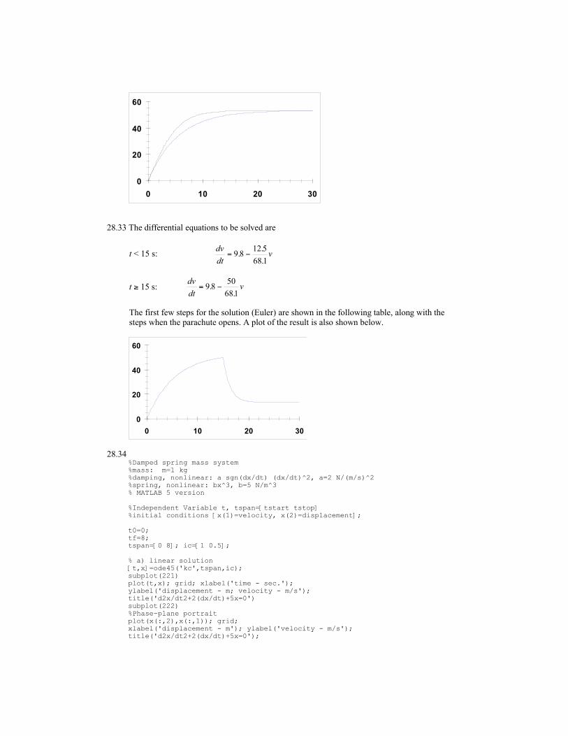
0
20
40
60
0 10 20 30
28.33 The differential equations to be solved are
t < 15 s:dv
dtv= −9 8
12 5
68 1.
.
.
t ≥ 15 s:dv
dtv= −9 8
50
681.
.
The first few steps for the solution (Euler) are shown in the following table, along with thesteps when the parachute opens. A plot of the result is also shown below.
0
20
40
60
0 10 20 30
28.34%Damped spring mass system%mass: m=1 kg%damping, nonlinear: a sgn(dx/dt) (dx/dt)^2, a=2 N/(m/s)^2%spring, nonlinear: bx^3, b=5 N/m^3% MATLAB 5 version
%Independent Variable t, tspan=[tstart tstop]%initial conditions [x(1)=velocity, x(2)=displacement];
t0=0;tf=8;tspan=[0 8]; ic=[1 0.5];
% a) linear solution [t,x]=ode45('kc',tspan,ic);subplot(221)plot(t,x); grid; xlabel('time - sec.');ylabel('displacement - m; velocity - m/s'); title('d2x/dt2+2(dx/dt)+5x=0')subplot(222)%Phase-plane portraitplot(x(:,2),x(:,1)); grid; xlabel('displacement - m'); ylabel('velocity - m/s');title('d2x/dt2+2(dx/dt)+5x=0');

% b) nonlinear spring [t,x]=ode45('nlk',tspan,ic);subplot(223)plot(t,x); grid; xlabel('time - sec.'); ylabel('displacement - m; velocity - m/s'); title('d2x/dt2+2(dx/dt)+5x^3=0')%Phase-plane portraitsubplot(224)plot(x(:,2),x(:,1)); grid; xlabel('displacement - m'); ylabel('velocity - m/s');title('d2x/dt2+2(dx/dt)+5x=0');pause
% c) nonlinear damping [t,x]=ode45('nlc',tspan,ic);subplot(221)plot(t,x); grid; xlabel('time - sec.'); ylabel('displacement - m; velocity - m/s'); title('d2x/dt2+2sign(dx/dt)(dx/dt)^2+5x=0')%Phase-plane portraitsubplot(222)plot(x(:,2),x(:,1)); grid; xlabel('displacement - m'); ylabel('velocity - m/s');title('d2x/dt2+2sign(dx/dt)(dx/dt)^2+5x=0');
% d) nonlinear damping and spring [t,x]=ode45('nlck',tspan,ic);subplot(223)plot(t,x); grid; xlabel('time - sec.'); ylabel('displacement - m; velocity - m/s'); title('d2x/dt2+2sign(dx/dt)(dx/dt)^2+5x^3=0')%Phase-plane portraitsubplot(224)plot(x(:,2),x(:,1)); grid; xlabel('displacement - m'); ylabel('velocity - m/s');title('d2x/dt2+2sign(dx/dt)(dx/dt)^2+5x^3=0');
Functions:
%Damped spring mass system - m d2x/dt2 + c dx/dt + k x =0%mass: m=1 kg % linear- c=2 N/(m/s)% linear- k=5 N/m%x(1)=velocity, x(2)=displacement
function dx=kc(t,x);dx=[-2*x(1)-5*x(2); x(1)]
%Damped spring mass system - m d2x/dt2 + c dx/dt + k x =0%mass: m=1 kg%damping: linear- c=2 N/(m/s)%spring: nonlinear- kx=bx^3, b=5 N/m^3
function dx=nlk(t,x);dx=[-2*x(1)-5*x(2).*x(2).*x(2); x(1)]
%Damped spring mass system - m d2x/dt2 + c dx/dt + k x =0%mass: m=1 kg%damping: nonlinear- c dx/dt = a sgn(dx/dt) (dx/dt)^2, a=2 N/(m/s)^2 %spring: linear- kx=5x%x(1)=velocity, x(2)=dispacement
function dx=nlc(t,x);dx(1)=-2*sign(x(1))*x(1)*x(1)-5*x(2);dx(2)= x(1);
%Damped spring mass system - m d2x/dt2 + c dx/dt + k x =0%mass: m=1 kg%damping: nonlinear- c dx/dt = a sgn(dx/dt) (dx/dt)^2, a=2 N/(m/s)^2 %spring: nonlinear- k x = bx^3, b=5 N/m^3%x(1)=velocity, x(2)=dispacement
function dx=nlck(t,x);dx=[-2*sign(x(1)).*x(1).*x(1)-5*x(2).*x(2).*x(2); x(1)]

0 2 4 6 8-1
-0.5
0
0.5
1
tim e - s ec .disp
lace
men
t - m
; vel
ocity
- m
/s d2x /dt2+2(dx /dt)+5x =0
-0.5 0 0.5 1-1
-0.5
0
0.5
1
displacem ent - m
velo
city
- m
/s
d2x /dt2+2(dx /dt)+ 5x=0
0 2 4 6 8-0.5
0
0.5
1
tim e - s ec .disp
lace
men
t - m
; vel
ocity
- m
/s d2x /dt2+ 2(dx /dt)+ 5x 3= 0
0 0.2 0.4 0.6 0.8-0.5
0
0.5
1
displacem ent - m
velo
city
- m
/s
d2x /dt2+2(dx /dt)+ 5x=0
0 2 4 6 8-1
-0.5
0
0.5
1
tim e - sec .disp
lace
men
t -
m;
velo
city
- m
/s d2x /dt2+2s ign(dx /dt)(dx /dt)2+ 5x=0
-0.5 0 0.5 1-1
-0.5
0
0.5
1
displacem ent - m
velo
city
- m
/s
d2x /dt2+2s ign(dx /dt)(dx /dt)2+5x= 0
0 2 4 6 8-1
-0.5
0
0.5
1
tim e - sec .disp
lace
men
t -
m;
velo
city
- m
/s d2x /dt2+ 2s ign(dx /dt)(dx /dt)2+ 5x3=0
-0.5 0 0.5 1-1
-0.5
0
0.5
1
displacem ent - m
velo
city
- m
/s
d2x /dt2+2s ign(dx /dt)(dx /dt)2+5x 3= 0
28.35%Forced damped spring-mass system w/ material damping%mass: m=2 kg%damping, nonlinear material: b sgn(dx/dt) abs(x), b=1 N/m%spring, linear: kx = 6x%forcing function: F=Fo(sin(wt)), Fo=2 N, w=0.5 rad/s

% MATLAB 5 version%Independent Variable t, tspan=[tstart tstop]%initial conditions [x(1)=velocity, x(2)=displacement];
tspan=[0 15]; ic=[0 1]; [t,x]=ode45('nlF',tspan,ic);
ts=0:.01:15;Sin=2*sin(0.5*ts);plot(t,x,ts,Sin,'--'); grid; xlabel('time - sec.');
ylabel('displacement - m; velocity - m/s; force - N'); title('non-linear, forced,damped spring-mass system, time response')
Function ‘n1F’:%Forced damped spring-mass system w/ material damping%mass: m=2 kg%damping, nonlinear air: b sgn(dx/dt) (dx/dt)^2, b=1 N/m%spring, linear: kx = 6x%forcing function: F=Fo(sin(wt), Fo=2 N, w=0.5 rad/s% x(1)= velocity, x(2)= displacement
function dx=nlF(t,x);dx=[-0.5*sign(x(1)).*x(1).*x(1)-3*x(2)+sin(0.5*t); x(1)]
0 5 10 15-2
-1.5
-1
-0.5
0
0.5
1
1.5
2
tim e - sec .
disp
lace
men
t -
m;
velo
city
- m
/s; f
orce
- N
non-linear, forced,dam ped spring-m ass sys tem , tim e respons e
28.36% ODE Boundary Value Problem% Tapered conical cooling fin % u[xx]+(2/x)(u[x]-pu)=0% BC. u(x=0)=0 u(x=1)=1% i=spatial index, from 1 to R% numbering for points is i=1 to i=R for (R-1) dx spaces% u(i=1)=0 and u(i=R)=1
R=21;%Constantsdx=1/(R-1);dx2=dx*dx;%Parametersp(1)=10; p(2)=20; p(3)=50; p(4)=100;%sizing matricesu=zeros(1,R); x=zeros(1,R);a=zeros(1,R); b=zeros(1,R); c=zeros(1,R); d=zeros(1,R);ba=zeros(1,R); ga=zeros(1,R);%Independent Variablex=0:dx:1;%Boundary Conditionsu(1)=0; u(R)=1;

for k=1:4; %/Coefficients b(2)=-2-2*p(k)*dx2/dx; c(2)=2; for i=3:R-2, a(i)=1-dx/(dx*(i-1)); b(i)=-2-2*p(k)*dx2/(dx*(i-1)); c(i)=1+1/(i-1); end a(R-1)=1-dx/(dx*(R-2)); b(R-1)=-2-2*p(k)*dx2/(dx*(R-2)); d(R-1)=-(1+1/(R-2));%Solution by Thomas Algorithm
ba(2)=b(2); ga(2)=d(2)/b(2); for i=3:R-1, ba(i)=b(i)-a(i)*c(i-1)/ba(i-1); ga(i)=(d(i)-a(i)*ga(i-1))/ba(i); end %back substitution step u(R-1)=ga(R-1); for i=R-2:-1:2, u(i)=ga(i)-c(i)*u(i+1)/ba(i); end %Plot plot(x,u) title('u[xx]+(2/x)(u[x]-pu)=0; u(x=0)=0, u(x=1)=1') xlabel('x -ND Length') ylabel('u - ND Temperature') hold onendgridhold offgtext('p=10');gtext('p=20');gtext('p=50');gtext('p=100');
0 0.1 0.2 0.3 0.4 0.5 0.6 0.7 0.8 0.9 10
0.1
0.2
0.3
0.4
0.5
0.6
0.7
0.8
0.9
1u[xx ]+ (2/x )(u[x ]-pu)=0; u(x= 0)= 0, u(x=1)= 1
x -ND Length
u -
ND
Tem
pera
ture
p=10
p= 20
p=50p=100
t v dvdt
0 0 9.8
0.1 0.98 9.620117
0.2 1.942012 9.443537
0.3 2.886365 9.270197
0.4 3.813385 9.100039
0.5 4.723389 8.933005

•••
14.9 50.01245 0.620036
15 50.07445 -26.9654
15.1 47.37791 -24.9855
15.2 44.87936 -23.1511
15.3 42.56425 -21.4513
15.4 40.41912 -19.8763
15.5 38.43149 -18.417
linear nonlinear analytical
t v dvdt v dvdt
0 0 9.8 0 9.8 0
0.1 0.98 9.620117 0.98 9.796686 0.971061
0.2 1.942012 9.443537 1.959669 9.786748 1.92446
0.3 2.886365 9.270197 2.938343 9.770206 2.860518
0.4 3.813385 9.100039 3.915364 9.747099 3.779552
0.5 4.723389 8.933005 4.890074 9.717481 4.681871
t T k11 T-end k21 phi1
0 0 1598 159.8 1602.005 1600.003
0.1 160.0003 1593.995 319.3997 1598 1595.997
0.2 319.6 1589.97 478.597 1593.975 1591.972
0.3 478.7972 1585.924 637.3897 1589.929 1587.927
0.4 637.5899 1581.859 795.7758 1585.863 1583.861
0.5 795.976 1577.772 953.7532 1581.777 1579.774
t T k11 T-end k21 phi1
0 90 -10 89 -9.8 -9.9
0.1 89.01 -9.802 88.0298 -9.60596 -9.70398
0.2 88.0396 -9.60792 87.07881 -9.41576 -9.51184
0.3 87.08842 -9.41768 86.14665 -9.22933 -9.32351
0.4 86.15607 -9.23121 85.23295 -9.04659 -9.1389
0.5 85.24218 -9.04844 84.33733 -8.86747 -8.95795
x v k11 k12 x v k21 k22 phi1 phi2
0.3 0 0 -312.5 0.3 -0.3125 -0.3125 -308.854 -0.15625 -310.677
0.299844 -0.31068 -0.31068 -308.713 0.299533 -0.61939 -0.61939 -304.787 -0.46503 -306.75
0.299379 -0.61743 -0.61743 -304.65 0.298761 -0.92208 -0.92208 -300.452 -0.76975 -302.551
0.298609 -0.91998 -0.91998 -300.318 0.297689 -1.2203 -1.2203 -295.856 -1.07014 -298.087
0.297539 -1.21806 -1.21806 -295.726 0.296321 -1.51379 -1.51379 -291.007 -1.36593 -293.366
t thet v k11 k12 thet v k21 k22 thet v k31 k32 thet v k41 k42 phi1 phi2
0 0.785 0.000 0.000 -5.692 0.785 -0.028 -0.028 -5.692 0.785 -0.028 -0.028 -5.691 0.785 -0.057 -0.057 -5.691 -0.028 -5.692
0.01 0.785 -0.057 -0.057 -5.691 0.785 -0.085 -0.085 -5.689 0.785 -0.085 -0.085 -5.688 0.784 -0.114 -0.114 -5.686 -0.085 -5.688
0.02 0.784 -0.114 -0.114 -5.686 0.784 -0.142 -0.142 -5.682 0.784 -0.142 -0.142 -5.682 0.783 -0.171 -0.171 -5.678 -0.142 -5.682
0.03 0.783 -0.171 -0.171 -5.678 0.782 -0.199 -0.199 -5.673 0.782 -0.199 -0.199 -5.672 0.781 -0.227 -0.227 -5.666 -0.199 -5.672
0.04 0.781 -0.227 -0.227 -5.666 0.780 -0.256 -0.256 -5.660 0.780 -0.256 -0.256 -5.659 0.778 -0.284 -0.284 -5.652 -0.256 -5.659
t (analytical) (Euler) didt
0 0.600000 0.600000 -0.768000
0.05 0.542902 0.561600 -0.768949
0.1 0.491238 0.523153 -0.759943
0.15 0.444491 0.485155 -0.741923
0.2 0.402192 0.448059 -0.716216
0.25 0.363918 0.412248 -0.684375

t (analytical) (Euler) didt
0 0.600000 0.600000 -1.200000
0.05 0.542902 0.540000 -1.080000
0.1 0.491238 0.486000 -0.972000
0.15 0.444491 0.437400 -0.874800
0.2 0.402192 0.393660 -0.787320
0.25 0.363918 0.354294 -0.708588
t i q k11 k12 imid qmid k21 k22 imid qmid k31 k32 iend qend k41 k42 phi1 phi20 -3.282 0.100 -134.37 -3.282 -3.617 0.092 -111.24 -3.617 -3.560 0.091 -110.7 -3.560 -3.835 0.082 -87.70 -3.835 -111.0 -3.578
0.005 -3.837 0.082 -87.485 -3.837 -4.055 0.073 -63.93 -4.055 -3.996 0.072 -64.01 -3.996 -4.157 0.062 -41.12 -4.157 -64.08 -4.016
0.01 -4.157 0.062 -40.917 -4.157 -4.259 0.052 -18.09 -4.259 -4.202 0.051 -18.72 -4.202 -4.251 0.041 2.976 -4.251 -18.59 -4.222
0.015 -4.250 0.041 3.159 -4.250 -4.242 0.030 24.25 -4.242 -4.189 0.030 23.16 -4.189 -4.134 0.020 42.736 -4.134 23.452
-4.208
0.02 -4.133 0.020 42.892 -4.133 -4.025 0.010 61.41 -4.025 -3.979 0.010 59.95 -3.979 -3.833 0.000 76.688 -3.833 60.383
-3.996
t i q k11 k12 imid qmid k21 k22 imid qmid k31 k32 iend qend k41 k42 phi1 phi20 0.000
00.000
00.000
00.000
00.000
00.000
00.093
40.000
00.004
70.000
00.093
20.004
70.009
30.000
50.183
70.009
30.092
80.0031
0.1 0.0093
0.0003
0.1843
0.0093
0.0185
0.0008
0.2729
0.0185
0.0229
0.0012
0.2709
0.0229
0.0364
0.0026
0.3533
0.0364
0.2709
0.0214
0.2 0.0364
0.0025
0.3539
0.0364
0.0541
0.0043
0.4311
0.0541
0.0579
0.0052
0.4273
0.0579
0.0791
0.0082
0.4953
0.0791
0.4277
0.0566
0.3 0.0791
0.0081
0.4958
0.0791
0.1039
0.0121
0.5555
0.1039
0.1069
0.0133
0.5504
0.1069
0.1342
0.0188
0.5985
0.1342
0.5510
0.1058
0.4 0.1342
0.0187
0.5989
0.1342
0.1642
0.0254
0.6361
0.1642
0.1660
0.0269
0.6300
0.1660
0.1972
0.0353
0.6538
0.1972
0.6308
0.1653
t p k1 pend k2 phi
0 5000 750 5375 786.0938 768.0469
0.5 5384.023 786.9276 5777.487 821.7039 804.3157
1 5786.181 822.4373 6197.4 855.4023 838.9198
1.5 6205.641 856.0284 6633.655 886.6772 871.3528
•••
18 18480.96 280.733 18621.33 256.7271 268.7301
18.5 18615.33 257.7616 18744.21 235.3885 246.575
19 18738.61 236.3663 18856.8 215.5715 225.9689
19.5 18851.6 216.4921 18959.84 197.2119 206.852
20 18955.02 198.0754 19054.06 180.2397 189.1575
t p k1 pend k2 phi0 5000 350 5175 362.25 356.125
0.5 5178.063 362.4644 5359.295 375.1506 368.80751 5362.466 375.3726 5550.153 388.5107 381.9417
1.5 5553.437 388.7406 5747.807 402.3465 395.54362 5751.209 402.5846 5952.501 416.6751 409.6299
•••
18 17622.69 1233.588 18239.48 1276.764 1255.17618.5 18250.28 1277.52 18889.04 1322.233 1299.876
19 18900.22 1323.015 19561.72 1369.321 1346.16819.5 19573.3 1370.131 20258.37 1418.086 1394.108
20 20270.36 1418.925 20979.82 1468.587 1443.756
t c1 c2 c3 dc1/dt dc2/dt dc3/dt
0 0 0 100 21.93515 0 -43.8703
0.1 2.193515 0 95.61297 19.41211 0.252723 -40.9834

0.2 4.134726 0.025272 91.51463 17.13425 0.473465 -38.3338
0.3 5.848151 0.072619 87.68125 15.07861 0.66542 -35.9004
0.4 7.356012 0.139161 84.09121 13.22439 0.83148 -33.664
0.5 8.678451 0.222309 80.72481 11.55268 0.974263 -31.607
z y w dydz dwdz
0 0 0 0 0.0036
1 0 0.0036 0.0036 0.003364
2 0.0036 0.006964 0.006964 0.003136
3 0.010564 0.0101 0.0101 0.002916
4 0.020664 0.013016 0.013016 0.002704
5 0.03368 0.01572 0.01572 0.0025
•••
26 0.676 0.0377 0.0377 0.000064
27 0.7137 0.037764 0.037764 0.000036
28 0.751464 0.0378 0.0378 0.000016
29 0.789264 0.037816 0.037816 0.000004
30 0.82708 0.03782 0.03782 0
z f(z) y w dydz dwdz
0 0 0 0 0 0
1 31.18357 0 0 0 0.002098
2 50.0099 0 0.002098 0.002098 0.003137
3 61.40481 0.002098 0.005235 0.005235 0.003581
4 68.08252 0.007333 0.008816 0.008816 0.003682
5 71.65313 0.016148 0.012498 0.012498 0.003583
•••
26 29.63907 0.700979 0.040713 0.040713 3.79E-05
27 27.89419 0.741693 0.040751 0.040751 2.01E-05
28 26.24164 0.782444 0.040771 0.040771 8.4E-06
29 24.67818 0.823216 0.04078 0.04078 1.97E-06
30 23.20033 0.863995 0.040782 0.040782 0
z y w dydz dwdz
0 0 0 0 0.0036
1 0 0.0036 0.0036 0.003364
2 0.0036 0.006964 0.006964 0.003136
3 0.010564 0.0101 0.0101 0.002916
4 0.020664 0.013016 0.013016 0.002704
5 0.03368 0.01572 0.01572 0.0025
•••
26 0.676 0.0377 0.0377 0.000064
27 0.7137 0.037764 0.037764 0.000036
28 0.751464 0.0378 0.0378 0.000016
29 0.789264 0.037816 0.037816 0.000004
30 0.82708 0.03782 0.03782 0
t x y Z
0 5 5 5
0.1 9.78147 17.07946 10.43947
0.2 17.70297 20.8741 35.89688

0.3 10.81088 -2.52924 39.30744
0.4 0.549577 -5.54419 28.07461
0.5 -3.16461 -5.84129 22.36888
0.6 -5.57588 -8.42037 19.92312
0.7 -8.88719 -12.6789 22.14149
0.8 -11.9142 -13.43 29.80001
0.9 -10.6668 -7.21784 33.39903
1 -6.84678 -3.43018 29.30716
0 2 30.1 1.887095 2.9355170.2 1.787897 2.8633010.3 1.701588 2.7851070.4 1.627287 2.7025360.5 1.564109 2.617016
0 2 30.1 1.886984 2.9353080.2 1.787729 2.8628990.3 1.701406 2.7845350.4 1.627125 2.7018210.5 1.56399 2.616185
t x y0 2 3
0.1 1.88 2.940.2 1.773968 2.8706160.3 1.681301 2.7937380.4 1.601231 2.7111530.5 1.532907 2.624496
t C Te
0 1 25
0.0625 0.941218 66.18648
0.125 0.885749 85.80247
0.1875 0.833497 93.93385
0.25 0.784309 96.02265
0.3125 0.738024 94.99472
0.375 0.694475 92.41801
0.4375 0.653506 89.12894
0.5 0.614963 85.57041
0.5625 0.578703 81.97385
0.625 0.54459 78.45733
0.6875 0.512497 75.07829
0.75 0.482304 71.86194
0.8125 0.453896 68.81648
0.875 0.427168 65.9413
0.9375 0.40202 63.23134
1 0.378358 60.67946
•••
x A x A x A x A
0 0.1
0.2 0.067208 1.2 0.009215 2.2 0.001263 3.2 0.000166
0.4 0.045169 1.4 0.006193 2.4 0.000848 3.4 0.000106

0.6 0.030357 1.6 0.004162 2.6 0.000569 3.6 6.23E-05
0.8 0.020402 1.8 0.002797 2.8 0.00038 3.8 2.88E-05
1 0.013712 2 0.00188 3 0.000253 4 0
t M m s dmdt
0 1000 8000 8 0
5 997.5 8000 8.02005 -0.2005
10 995 7998.997 8.039193 -0.39193
15 992.5 7997.038 8.057469 -0.57469
20 990 7994.164 8.074914 -0.74914
25 987.5 7990.419 8.091563 -0.91563
t cin c k1 cend cin-end k2 phi0 0 10 -0.5 9 9.063462 0.003173 -0.248412 9.063462 9.503173 -0.02199 9.459202 16.484 0.35124 0.1646274 16.484 9.832427 0.332579 10.49758 22.55942 0.603092 0.4678356 22.55942 10.7681 0.589566 11.94723 27.53355 0.779316 0.6844418 27.53355 12.13698 0.769829 13.67664 31.60603 0.89647 0.833149
10 31.60603 13.80328 0.890138 15.58355 34.94029 0.967837 0.928987
t c1 c2 c3 c4 c5 dc1dt dc2dt dc3dt dc4dt dc5dt
0 0.0000 0.0000 0.0000 0.0000 0.0000 1.0000 0.0000 5.0000 0.0000 0.0000
1 1.0000 0.0000 5.0000 0.0000 0.0000 0.8600 0.2000 3.6250 0.5625 0.0300
2 1.8600 0.2000 8.6250 0.5625 0.0300 0.7396 0.3320 2.6331 0.8726 0.0600
3 2.5996 0.5320 11.2581 1.4351 0.0900 0.6361 0.4135 1.9173 1.0176 0.0885
4 3.2357 0.9455 13.1754 2.4528 0.1785 0.5470 0.4580 1.4004 1.0575 0.1147
5 3.7827 1.4035 14.5758 3.5102 0.2933 0.4704 0.4758 1.0267 1.0328 0.1380
•••
76 7.1428 7.1426 18.8311 13.0962 7.0053 0.0000 0.0000 0.0000 0.0018 0.0082
77 7.1428 7.1426 18.8311 13.0980 7.0135 0.0000 0.0000 0.0000 0.0017 0.0078
78 7.1428 7.1427 18.8311 13.0997 7.0213 0.0000 0.0000 0.0000 0.0016 0.0073
79 7.1428 7.1427 18.8311 13.1013 7.0286 0.0000 0.0000 0.0000 0.0015 0.0069
80 7.1428 7.1427 18.8311 13.1028 7.0354 0.0000 0.0000 0.0000 0.0014 0.0064
t c k1 cmid k2 cmid k3 cend k4 phi0 10 2 20 1.5 17.5 1.625 26.25 1.1875 1.572917
10 25.72917 1.213542 31.79688 0.910156 30.27995 0.986003 35.58919 0.72054 0.954420 35.27317 0.736342 38.95487 0.552256 38.03445 0.598278 41.25594 0.437203 0.57910230 41.06419 0.446791 43.29814 0.335093 42.73965 0.363017 44.69436 0.265282 0.35138240 44.57801 0.2711 45.93351 0.203325 45.59463 0.220268 46.78069 0.160965 0.21320850 46.71009 0.164495 47.53257 0.123371 47.32695 0.133652 48.04662 0.097669 0.129369
t c k1 c k2 phi0 10 2 30 1 1.5
10 25 1.25 37.5 0.625 0.937520 34.375 0.78125 42.1875 0.390625 0.58593830 40.23438 0.488281 45.11719 0.244141 0.36621140 43.89648 0.305176 46.94824 0.152588 0.22888250 46.1853 0.190735 48.09265 0.095367 0.143051

CHAPTER 32
32.1 First equation
6 075 3 2 262 50 1. . .c c− =
Middle equations (i = 1 to 8)
− + − =− +2 1 3 45 11 01 1. . .c c ci i i
Last equation
− + =3 2 3 45 08 9. .c c
The solution is
32.2 Element equation: (See solution for Prob. 31.4 for derivation of element equation.)
a a
a a
c
c
b
b
11 12
21 22
1
2
1
2
=
a11
2
2 5
1
2
0 2
22 5 055= − + =
.
.( . ) . a12
2
2 5
1
20 3=
−+ = −
..
a 21
2
2 5
1
21 3=
−− = −
.. a 22
2
2 5
1
2
0 2
22 5 155= + + =
.
.( . ) .
bdc
dxx1 12= − ( ) b
dc
dxx2 22= ( )
Assembly:
0 55 0 3
13 2 1 0 3
1 3 2 1 0 3
1 3 2 1 0 3
1 3 155
0
0
0
0
1
2
3
4
1
2
. .
. . .
. . .
. . .
. .
( )
( )
−
− −
− −
− −
−
=
−
c
c
c
c
c
dc
dxx
dc
dxx
Boundary conditions:
Inlet:
Uc Uc Ddc
dx
dc
dx
Uc Uc
D
in
in
= −
=−
0
0
0
0
( )
( )
Substitute into first equation

0 55 0 3 100
155 0 3 100
0 1 0
0 1
. .
. .
c c c
c c
− = −
− =
Outlet:
dc
dx( )10 0=
Solution:
c0 = 74.4 c1 = 51.08 c2 = 35.15 c3 = 24.72 c2 = 20.74
32.3 According to Fick’s first law, the diffusive flux is
J x Ddc
dxx( ) ( )= −
where J(x) = flux at position x. If c has units of g/m3, D has units of m2/d and x is measuredin m, flux has units of g/m2/d. In addition, there will be an advective flux which can becalculated as
J x Uc x( ) ( )=
Finite divided differences can be used to approximate the derivatives. For example, for thepoint at the beginning of the tank, a forward difference can be used to calculate
dc
dx( )
. .
..0
52 47 76 44
2 50 9588≅
−= −
g / m
m
3
Thus, the flux at the head of the tank is
J x( ) ( . ) ( . ) . . .= − − + = + =2 0 9588 1 76 44 19 176 76 44 95 616 g / m
m
3
The remasinder of the values can be calculated in a similar fashion using centered (middlenodes) and backward differences (the end node):

32.4 Segmentation scheme:
4 0
4 0
4 0
1 0 0 1 0 0 1 0 0
1 , 0 2 , 0 3 , 0
1 , 2 2 , 2 3 , 2 4 , 2 5 , 2 6 , 2
1 , 1 2 , 1 3 , 1 4 , 1 5 , 1 6 , 1
d c /d y = 0
d c /d y = 0
dc/
dx
= 0
Nodes 1,1 through 5,1
0 42
50 4
2
50 2
1 1
2
1 1
2. . .
, , , , , ,
,
c c c c c cc
i j i j i j i j i j i j
i j
+ − + +− ++
− +−
Collecting terms gives
0 264 0 016 0 016 0 016 0 016 01 1 1 1. . . . ., , , , ,c c c c ci j i j i j i j i j− − − − =+ − + +
Node 6,1 would be modified to reflect the no flow condition in x and the Dirichlet conditionat 6,0:
0 264 0 032 0 016 0 016 100 06 1 5 1 6 2. . . . ( ), , ,c c c− − − =
The nodes along the upper edge (1,2 through 5,2) would be generally written to reflect theno-flow condition in y as
0 264 0 016 0 016 0 032 01 1 1. . . ., , , ,c c c ci j i j i j i j− − − =+ − +
The node at the upper right edge (6,2) would be generally written to reflect the no-flowcondition in x and y as
0 264 0 032 0 032 06 2 5 2 6 1. . ., , ,c c c− − =
Finally, the nodes along the lower edge (1,0 through 3,0) would be generally written toreflect the no-flow condition in y as
0 264 0 016 0 016 0 032 01 1 1. . . ., , , ,c c c ci j i j i j i j− − − =+ − +
These equations can be solved for

32.5 For simplicity, we will use a very coarse grid to solve this problem. Thus, we place nodes asin the following diagram.
oil
water
v10o
v8o
v6o v6w
v4w
v2w
v0w
x
0
A simple explicit solution can be developed by substituting finite-differences for the secondderivative terms in the motion equations. This is done for the three non-boundary nodes,
dv
dt
v v v
x
ww
w w w2 0 2 4
2
2=
− +µ
∆
dv
dt
v v v
x
ww
w w w4 2 4 6
2
2=
− +µ
∆
dv
dt
v v v
x
oo
o o o8 6 8 10
2
2=
− +µ
∆
These three equations have 7 unknowns (v0w, v2w, v4w, v6w, v6o, v8o, v10o). The boundaryconditions at the plates effectively specify v0w = 0 and v10o = 7. The former is called a “noslip” condition because it specifies that the velocity at the lower plate is zero.
The relationships at the oil-water interface can be used to used to eliminate two of theremaining unknowns. The first condition states that
v6o = v6w (i)
The second can be rearrange to yield
vv v
wo o w w
o w
68 4=+
+
µ µ
µ µ(ii)
These, along with the wall boundary conditions can be substituted into the differentialequations
dv
dt
v v
x
ww
w w2 2 4
2
2=
− +µ
∆
dv
dt
v v
x
ww
w wo o w w
o w4
2 48 4
2
2
=
− ++
+µ
µ ν µ ν
µ µ
∆

dv
dt
v
x
oo
o o w w
o w
o
8
8 48
2
2 7
=
+
+− +
µ
µ ν µ ν
µ µ
∆
These equations can now be integrated to determine the velocities as a function of time.Equations (i) and (ii) can be used to determine v6o and v6w. The results are plotted below:
0
4
8
0 2 4 6 8 10
t = 1.5 s
t = 0.5 s
t = 1.0 s
32.6 Using a similar approach to Sec. 32.2, the following nodal equation can be developed fornode 11:
4 121954 121954 0 78049 0 78049 0 35786611 12 10 12 01u u u u u− − − − =. . . . .
Similar equations can be written for the other nodes and the resulting equations solved for
A graphical comparison of the results from Sec. 32.2 can be made with these results bydeveloping a plot along the y dimension in the middle of the plate:
-0.6
-0.3
0
0 0.5 1 1.5 2
These results can then be used as input to the right-hand side of Eq. 32.14 and the resultingsimultaneous equations solved for
Again the comparison is good

0
0.04
0.08
0.12
0 0.5 1 1.5 2
32.7 Grid scheme
0, 2 1, 2 2, 2 3, 2
0, 1 1, 1 2, 1 3, 1
0, 0 1, 0 2, 0
All nodes in the above scheme can be modeled with the following general differenceequation
h h h
x
h h h
y
i j i j i j i j i j i j+ − + −− ++
− +=1 1
2
1 1
2
2 20
, , , , , ,
∆ ∆
Node 0,0:
h h h
x
h h h
y
1 0 0 0 1 0
2
0 1 0 0 0 1
2
2 20
, , , , , ,− ++
− +=− −
∆ ∆
The external nodes can be approximated with finite differences
dh
dy
h h
y
h h ydh
dyh
=−
= − =
−
−
0 1 0 1
0 1 0 1 0 1
2
2
, ,
, , ,
∆
∆
dh
dx
h h
x
h h xdh
dxh h
=−
= − = − = −
−
−
1 0 1 0
1 0 1 0 1 0 1 0
2
2 2 1 1 2
, ,
, , , ,( )( )
∆
∆
which can be substituted into the difference equation to give

2 2 2 2 20
4 2 2 2
1 0 0 0
2
0 1 0 0
2
0 0 1 0 0 1
h h
x
h h
y
h h h
, , , ,
, , ,
− −+
−=
− − = −
∆ ∆
Node 1,0:
4 2 01 0 1 1 0 0 2 0h h h h, , , ,− − − =
Node 2,0:
4 2 2 02 0 1 0 2 1h h h, , ,− − =
Node 0,1:
4 2 20 1 1 1 0 0 0 2h h h h, , , ,− − − = −
Node 1,1:
4 01 1 1 0 0 1 1 2 2 1h h h h h, , , , ,− − − − =
Node 2,1:
4 02 1 1 1 2 2 3 1 2 0h h h h h, , , , ,− − − − =
Node 0,2:
4 2 2 20 2 0 1 1 2h h h, , ,− − = −
Node 1,2:
4 2 01 2 0 2 2 2 1 1h h h h, , , ,− − − =
Node 2,2:
4 2 202 2 1 2 2 1h h h, , ,− − =
The equations can be solved simultaneously for
More refined results can be obtained by using a finer grid spacing.
32.8 The fluxes can be determined using finite divided differences as
32.9 Because of the equi-spaced grid, the domain can be modeled with simple Laplacians. Theresulting solution is
32.10 A convenient segmentation scheme can be developed as

Simple Laplacians reflecting the boundary conditions can be developed and solved for
32.11 The system to be solved is
2 7 2
2 2 75 0 75
0 75 2 25 15
15 15
0
0
0
2
1
2
3
4
.
. .
. . .
. .
−
− −
− −
−
=
x
x
x
x
which can be solved for x1 = 2.857, x2 = 3.857, x3 = 6.5238, and x4 = 7.857.
32.12 The system to be solved is
0 6 0 4
0 4 18 14
14 2 1 0 7
0 7 16 0 9
0 9 0 9
0
0
0
0
1
1
2
3
4
5
. .
. . .
. . .
. . .
. .
−
− −
− −
− −
−
=
x
x
x
x
x
which can be solved for x1 = 5, x2 = 7.5, x3 = 8.214286, x4 = 9.64286, and x5 = 10.75397.
32.13 Substituting the Crank-Nicolson finite difference analogues to the derivatives
t
uu
t
u
x
uuu
x
uuu
x
u
nini
nininininini
∆
−=
∂
∂
∆
+−+
∆
+−=
∂
∂
+
−++−+++
,1,
2
,1,,1
2
1,11,1,1
2
2
2
1
into the governing equations gives the following finite difference equations:
[ ] [ ]
[ ] [ ] 12
12222
2
10221221
,1,
2
,11,11,
2
1,1
,1,
2
,11,11,
2
1,1
≤≤−
∆
∆−+−=+
∆
∆−−+
≤≤−
∆
∆−+−=+
∆
∆−−+
+−++++−
+−++++−
xruut
xrruuru
t
xrur
xuut
xuuu
t
xu
nininininini
nininininini
Substitute for the end point boundary conditions to get the end point finite difference equations.Substitute the first order Crank Nicolson analogues to the derivatives

∆
−+
∆
−=
∂
∂ −++−++
r
uu
r
uu
r
u nininini
222
1 ,1,11,11,1 into the midpoint boundary condition and get
)()( ,11,1,11,1,11,1,11,1 nLnLnLnLnLb
nLb
nLa
nLa uuruuuuruu +++=+−++++++ +++=+++
where au and bu are fictitious points located in the opposite side of the midpoint from their
half. Write out the two finite difference equations from above for the point i = L (the midpoint)then combine these two equations with the midpoint boundary condition to obtain the midpointfinite difference equation:
[ ] [ ] nLnLnLnLnLnL urut
xruuu
t
xru ,1,
2
,11,11,
2
1,1 )1(4)1(2224)1(22 +−++++− +−
∆
∆−++−=+
∆
∆−+−+
%PDE Parabolic Problem - Transient Heat conduction in a composite rod% u[xx]=u[t] 0<x<0.5% r(u[xx])=u[t] 0.5<x<1% BC u(0,t)=1 u(1,t)=1% u[x]=r(u[x]) x=0.5% IC u(x,0)=0 0<x<1% i=spatial index, from 1 to imax % R = no. of x points (R=21 for 20 dx spaces)% n=time index from 1 to N% N = no. of time steps,% Crank-Nicolson Formulation
R=41; %(imax must be odd for point L to be correct)N=69; % last time step = nmax+1L=(R-1)/2+1; % L = midpoint of point no. (for R=41, L=21) % Constants
r=0.01;dx=1/(R-1);
dx2=dx*dx;dt=dx2; % Setting dt to dx2 for good stabilility and results
% Independent space variablex=0:dx:1;
% Sizing matrices
u=zeros(R,N+1); t=zeros(1,N+1);a=zeros(1,R); b=zeros(1,R);
c=zeros(1,R); d=zeros(1,R);ba=zeros(1,R); ga=zeros(1,R);up=zeros(1,R);
% Boundary Conditions at t=0 u(1,1)=1; u(R,1)=1;
% Time step loop% n=1 represents 0 time, next time = n+1
t(1)=0;for n=1:N
t(n+1)=t(n)+dt;
% Boundary conditions & Constantsu(1,n+1)=1;u(R,n+1)=1;dx2dt=dx2/dt;

% coefficients b(2)=-2-2*dx2dt; c(2)=1; d(2)=(2-2*dx2dt)*u(2,n)-u(3,n)-2; for i=3:L-1 a(i)=1; b(i)=-2-2*dx2dt; c(i)=1; d(i)=-u(i-1,n)+(2-2*dx2dt)*u(i,n)-u(i+1,n); end
a(L)=2;b(L)=-2*(1+r)-4*dx2dt;c(L)=2*r;
d(L)=-2*u(L-1,n)+(2*(1+r)-4*dx2dt)*u(L,n)-2*r*u(L+1,n);
for i=L+1:R-2 a(i)=r; b(i)=-2*r-2*dx2dt; c(i)=r; d(i)=-r*u(i-1,n)+(2*r-2*dx2dt)*u(i,n)-r*u(i+1,n); end a(R-1)=r; b(R-1)=-2*r-2*dx2dt; d(R-1)=-r*u(R-2,n)+(2*r-2*dx2dt)*u(R-1,n)-2*r;
% Solution by Thomas Algorithm ba(2)=b(2); ga(2)=d(2)/b(2); for i=3:R-1 ba(i)=b(i)-a(i)*c(i-1)/ba(i-1); ga(i)=(d(i)-a(i)*ga(i-1))/ba(i); end
% Back substitution step u(R-1,n+1)=ga(R-1); for i=R-2:-1:2 u(i,n+1)=ga(i)-c(i)*u(i+1,n+1)/ba(i); end dt=1.1*dt;
end % end of time step loop
% Plot% Storing plot value of u as up, at every 5 time steps% j=time index% i=space index
for j=5:5:N+1for i=1:R
up(i)=u(i,j);endplot(x,up)hold on
end
gridtitle('u[xx]=u[t] 0<x<0.5; r(u[xx])=u[t] 0.5<x<1; u(0,t)=1, u(1,t)=1,u(x,0)=0; u[x]=r(u[x]) x=0.5')xlabel('x - ND Space')ylabel('u - ND Temperature')hold offgtext('r=0.01')
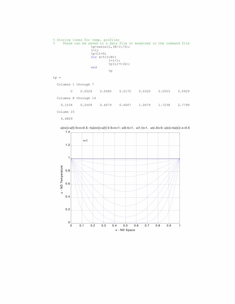
% Storing times for temp. profiles% These can be saved in a data file or examined in the command file
tp=zeros(1,(N-1)/5);i=1;tp(1)=0;for k=5:5:N+1
i=i+1;tp(i)=t(k);
endtp
tp =
Columns 1 through 7
0 0.0029 0.0085 0.0175 0.0320 0.0553 0.0929
Columns 8 through 14
0.1534 0.2509 0.4079 0.6607 1.0679 1.7238 2.7799
Column 15
4.4809
0 0.1 0.2 0.3 0.4 0.5 0.6 0.7 0.8 0.9 10
0.2
0.4
0.6
0.8
1
1.2
1.4u[xx ]= u[t] 0<x< 0.5; r(u[xx ])= u[t] 0.5< x<1; u(0,t)=1, u(1,t)= 1, u(x ,0)= 0; u[x ]= r(u[x ]) x= 0.5
x - ND S pace
u - N
D T
empe
ratu
re
r=1

0 0.1 0.2 0.3 0.4 0.5 0.6 0.7 0.8 0.9 10
0.2
0.4
0.6
0.8
1
1.2
1.4u[xx ]= u[t] 0<x < 0.5; r(u[xx ])= u[t] 0.5< x< 1; u(0,t)= 1, u(1,t)= 1, u(x ,0)= 0; u[x ]= r(u[x ]) x = 0.5
x - ND S pac e
u -
ND
Tem
pera
ture
r= 0.1
0 0.1 0.2 0.3 0.4 0.5 0.6 0.7 0.8 0.9 10
0.1
0.2
0.3
0.4
0.5
0.6
0.7
0.8
0.9
1u[xx ]= u[t] 0<x < 0.5; r(u[xx ])= u[t] 0.5< x< 1; u(0,t)= 1, u(1,t)= 1, u(x ,0)= 0; u[x ]= r(u[x ]) x = 0.5
x - ND S pac e
u -
ND
Tem
pera
ture
r= 0.01

0 0.1 0.2 0.3 0.4 0.5 0.6 0.7 0.8 0.9 10
0.1
0.2
0.3
0.4
0.5
0.6
0.7
0.8
0.9
1u[xx ]= u[t] 0<x < 0.5; r(u[xx ])= u[t] 0.5< x< 1; u(0,t)= 1, u(1,t)= 1, u(x ,0)= 0; u[x ]= r(u[x ]) x = 0.5
x - ND S pac e
u -
ND
Tem
pera
ture
r= 0.001
0 0.1 0.2 0.3 0.4 0.5 0.6 0.7 0.8 0.9 10
0.2
0.4
0.6
0.8
1
1.2
1.4u[xx ]= u[t] 0<x < 0.5; r(u[xx ])= u[t] 0.5< x< 1; u(0,t)= 1, u(1,t)= 1, u(x ,0)= 0; u[x ]= r(u[x ]) x = 0.5
x - ND S pac e
u -
ND
Tem
pera
ture r= 0

32.14


99.27296 99.15714 98.55306 96.07795 85.75874 69.00866 5099.38879 99.40126 99.48858 100 88.97417 70.13795 5099.47967 99.57055 100 100 100 72.56898 5099.38879 99.40126 99.48858 100 88.97417 70.13795 5099.27296 99.15714 98.55306 96.07795 85.75874 69.00866 50
25 40 40 30
10 21.87149 24.04033 20 15
10 13.44564 14.28983 12.63401 10 7.5
10 7.62124 7.039322 6.246222 5.311556 5
5 0 0 0 0 2.5
dh/dx
1.040287 1.106512 1.311258 1.4497791.014349 1.057395 1.344371 1.5883
0.931015 0.778698 0.62638
dh/dy
0.040287 0.066225 0.138521 00.054636 0.109272 0.38245 0
0.068985 0.152318 0.62638
dh/dn
1.041067 1.108492 1.318555 1.4497791.015819 1.063026 1.397713 1.5883
0.933568 0.793455 0.885835
θ (radians)
0.038707 0.059779 0.105249 00.053811 0.102975 0.277161 0
0.073961 0.193167 0.785398
θ (degrees)
2.217773 3.425088 6.030345 03.083137 5.90002 15.88014 0
4.237646 11.06765 45
16.3372 17.37748 18.55022 2016.29691 17.31126 18.4117 20
16.22792 17.15894 17.78532
0 0 0 0 0
0 0.052697 0.072156 0.052697 0
0 0.082316 0.113101 0.082316 0
0 0.082316 0.113101 0.082316 0
0 0.052697 0.072156 0.052697 0
0 0 0 0 0
0 0 0 0 0
0 -0.27719 -0.35074 -0.27719 0
0 -0.39124 -0.50218 -0.39124 0
0 -0.39124 -0.50218 -0.39124 0
0 -0.27719 -0.35074 -0.27719 0
0 0 0 0 0
20 1.387741 0.113952 0.155496 0.864874 0.951623 0.95896220 1.391891 0.168488 0.793428 6.581653 6.938975 6.959813
20 1.409973 0.48078 6.185917 100 100 100
c dcdx J-diff J-adv J76.44 -9.588 19.176 76.44 95.616
52.47 -8.076 16.152 52.47 68.622
36.06 -5.484 10.968 36.06 47.028
25.05 -3.394 6.788 25.05 31.838
19.09 -2.384 4.768 19.09 23.858

c0 76.53 c5 29.61c1 63.25 c6 24.62c2 52.28 c7 20.69c3 43.22 c8 17.88c4 35.75 c9 16.58

CHAPTER 25
25.1 The analytical solution can be derived by separation of variables
dy
yx dx∫ ∫= −2 12.
ln .yx
x C= − +3
312
Substituting the initial conditions yields C = 0. Taking the exponential give the final result
y e
xx
=−
3
31.2
The result can be plotted as
0
1
2
0 1 2
25.2 Euler’s method with h = 0.5
x y dy/dx0 1 -1.2
0.5 0.4 -0.38
1 0.21 -0.042
1.5 0.189 0.19845
2 0.288225 0.80703
Euler’s method with h = 0.25 gives
x y dy/dx0 1 -1.2
0.25 0.7 -0.79625
0.5 0.500938 -0.47589
0.75 0.381965 -0.2435
1 0.321089 -0.06422
1.25 0.305035 0.110575
1.5 0.332679 0.349312
1.75 0.420007 0.782262
2 0.615572 1.723602
The results can be plotted along with the analytical solution as

0
1
2
0 1 2
25.3 For Heun’s method, the value of the slope at x = 0 can be computed as −0.6 which can be used tocompute the value of y at the end of the interval as
y( . ) ( . ( )) . .0 5 1 0 12 1 0 5 0 4= + − =
The slope at the end of the interval can be computed as
y ' ( . ) . ( . ) . ( . ) .0 5 0 4 0 5 12 0 4 0 382= − = −
which can be averaged with the initial slope to predict
y( . ). .
. .0 5 10 6 0 38
20 5 0 605= +
− −=
This formula can then be iterated to yield
j yij
εa 0 0.4
1 0.605 33.9
2 0.5563124 8.75
3 0.5678757 2.036
4 0.5651295 0.4859
The remaining steps can be implemented with the result
xi yi
0.5 0.5651295
1.0 0.4104059
1.5 0.5279021
2.0 2.181574
The results along with the analytical solution are displayed below:

0
1
2
0 1 2
25.4 The midpoint method with h = 0.5
x y dy/dx ym dy/dx-mid
0 1 -1.2 0.7 -0.79625
0.5 0.601875 -0.57178 0.45893 -0.29257
1 0.455591 -0.09112 0.432812 0.156894
1.5 0.534038 0.56074 0.674223 1.255741
2 1.161909 3.253344 1.975245 7.629383
with h = 0.25 gives
x y dy/dx ym dy/dx-mid
0 1 -1.2 0.85 -1.00672
0.25 0.74832 -0.85121 0.641919 -0.68003
0.5 0.578312 -0.5494 0.509638 -0.41249
0.75 0.47519 -0.30293 0.437323 -0.18996
1 0.4277 -0.08554 0.417007 0.027366
1.25 0.434541 0.157521 0.454231 0.313703
1.5 0.512967 0.538615 0.580294 0.835986
1.75 0.721963 1.344657 0.890046 2.061012
2 1.237216 3.464206 1.670242 5.537897
The results can be plotted along with the analytical solution as
0
1
2
0 1 2

25.5 The 4th-order RK method with h = 0.5 gives
x y k1 ym k2 ym k3 ye k4 phi
0 1 -1.2 0.7 -0.79625 0.800938 -0.91107 0.544467 -0.51724 -0.85531
0.5 0.572344 -0.54373 0.436412 -0.27821 0.50279 -0.32053 0.412079 -0.08242 -0.30394
1 0.420375 -0.08407 0.399356 0.144767 0.456567 0.165505 0.503128 0.528284 0.177459
1.5 0.509104 0.534559 0.642744 1.197111 0.808382 1.505611 1.26191 3.533348 1.578892
2 1.29855 3.635941 2.207535 8.526606 3.430202 13.24915 7.923127 40.01179 14.53321
0
1
2
0 1 2
25.6 (a) The analytical solution can be derived by separation of variables
dy
yx dx∫ ∫= +1
22
2
y xx
C= + +
Substituting the initial conditions yields C = 2. Substituting this value and solving for y gives thefinal result
yx x
=+ +( )2 22 4
16
The result can be plotted as
0
2
4
0 0.5 1
(b) Euler’s method with h = 0.5
x y dy/dx

0 1 1
0.5 1.5 1.837117
1 2.418559 3.110343
Euler’s method with h = 0.25 gives
x y dy/dx0 1 1
0.25 1.25 1.397542
0.5 1.599386 1.897002
0.75 2.073636 2.520022
1 2.703642 3.288551
The results can be plotted along with the analytical solution as
0
2
4
0 0.5 1
(c) For Heun’s method, the first step along with the associated iterations is
j yij
εa0 1.500000
1 1.709279 12.243720
2 1.740273 1.780954
3 1.744698 2.536284E-01
The remaining steps can be implemented with the result
xi yi
0.00E+00 15.00E-01 1.7446981 3.122586
The results along with the analytical solution are displayed below:

0
2
4
0.0 0.5 1.0
(d) The midpoint method with h = 0.5
x y dy/dx ym dy/dx-mid0 1 1 1.25 1.397542
0.5 1.698771 1.955054 2.187535 2.588305
1 2.992924 3.460014 3.857927 4.419362
with h = 0.25 gives
x y dy/dx ym dy/dx-mid0 1 1 1.125 1.193243
0.25 1.298311 1.424293 1.476347 1.670694
0.5 1.715984 1.964934 1.961601 2.275929
0.75 2.284966 2.645318 2.615631 3.032421
1 3.043072 3.48888 3.479182 3.96367
The results can be plotted along with the analytical solution as
0
2
4
0 0.5 1
(e) The 4th-order RK method with h = 0.5 gives
x y k1 ym k2 ym k3 ye k4 phi0 1 1 1.25 1.397542 1.349386 1.452038 1.726019 1.970671 1.444972
0.5 1.722486 1.968653 2.214649 2.604297 2.37356 2.696114 3.070543 3.504593 2.679011
1 3.061992 3.499709 3.936919 4.464376 4.178086 4.599082 5.361533 5.788746 4.569229

0
2
4
0 0.5 1
25.7 The second-order ODE is transformed into a pair of first-order ODEs as in
dy
dxz y =
dz
dxx y z =
=
= −
( )
( )
0 2
0 0
(a) The first few steps of Euler’s method are
x y z dy/dx dz/dx0 2 0 0 -2
0.1 2 -0.2 -0.2 -1.90.2 1.98 -0.39 -0.39 -1.780.3 1.941 -0.568 -0.568 -1.6410.4 1.8842 -0.7321 -0.7321 -1.48420.5 1.81099 -0.88052 -0.88052 -1.31099
(b) For Heun (without iterating the corrector) the first few steps are
x y z dy/dx dz/dx yend zend dy/dx dz/dx ave slope0 2 0 0 -2 2 -0.2 -0.2 -1.9 -0.1
0.1 1.99 -0.195 -0.195 -1.89 1.9705 -0.384 -0.384 -1.7705 -0.28950.2 1.96105 -0.37803 -0.37803 -1.76105 1.923248 -0.55413 -0.55413 -1.62325 -0.466080.3 1.914442 -0.54724 -0.54724 -1.61444 1.859718 -0.70868 -0.70868 -1.45972 -0.627960.4 1.851646 -0.70095 -0.70095 -1.45165 1.781551 -0.84611 -0.84611 -1.28155 -0.773530.5 1.774293 -0.83761 -0.83761 -1.27429 1.690532 -0.96504 -0.96504 -1.09053 -0.90132
Both results are plotted below:
-2
0
2
4
0 2 4
y
z
Heun
Euler
x
25.8 The second-order ODE is transformed into a pair of first-order ODEs as in

dy
dtz y =
dz
dtz y z =
=
= − −
( )
( )
0 4
05 5 0 0.
The results for the 4th-order RK method are tabulated and plotted below:
t y z k11 k12 ymid zmid k21 k22 ymid zmid k31 k32 yend zend k41 k42 phi1 phi2
0 4.0000 0.0000 0.00 -20.00 4.00 -5.00 -5.00 -17.50 2.75 -4.38 -4.38 -11.56 1.81 -1.78 -1.78 -8.17 -3.42 -14.38
0.5 2.2891 -7.1914 -7.19 -7.85 0.49 -9.15 -9.15 2.12 0.00 -6.66 -6.66 3.33 -1.04 3.95 3.95 3.23 -5.81 1.05
1 -0.6167 -6.6682 -6.67 6.42 -2.28 -5.06 -5.06 13.95 -1.88 -3.18 -3.18 11.00 -2.21 4.89 4.89 8.59 -3.05 10.82
1.5 -2.1393 -1.2584 -1.26 11.33 -2.45 1.57 1.57 11.48 -1.75 1.61 1.61 7.92 -1.33 1.82 1.82 5.75 1.16 9.32
2 -1.5614 3.3995 3.40 6.11 -0.71 4.93 4.93 1.09 -0.33 3.67 3.67 -0.19 0.28 -1.66 -1.66 -0.55 3.16 1.23
2.5 0.0172 4.0139 4.01 -2.09 1.02 3.49 3.49 -6.85 0.89 2.30 2.30 -5.60 1.17 -2.78 -2.78 -4.45 2.14 -5.24
3 1.0852 1.3939 1.39 -6.12 1.43 -0.14 -0.14 -7.10 1.05 -0.38 -0.38 -5.06 0.89 -1.45 -1.45 -3.75 -0.18 -5.70
3.5 0.9945 -1.4562 -1.46 -4.24 0.63 -2.52 -2.52 -1.89 0.37 -1.93 -1.93 -0.86 0.03 0.56 0.56 -0.43 -1.63 -1.70
4 0.1790 -2.3048 -2.30 0.26 -0.40 -2.24 -2.24 3.11 -0.38 -1.53 -1.53 2.67 -0.59 1.51 1.51 2.17 -1.39 2.33
4.5 -0.5150 -1.1399 -1.14 3.15 -0.80 -0.35 -0.35 4.18 -0.60 -0.10 -0.10 3.07 -0.56 1.02 1.02 2.31 -0.17 3.32
5 -0.6001 0.5213 0.52 2.74 -0.47 1.21 1.21 1.75 -0.30 0.96 0.96 1.01 -0.12 -0.09 -0.09 0.65 0.79 1.49
-8
-4
0
4
8
0 2 4
y
z
t
25.9 (a) The Heun method without iteration can be implemented as in the following table:
t y k1 yend k2 phi
0 1 0 1 0.009967 0.004983
0.1 1.000498 0.009972 1.001496 0.039489 0.02473
0.2 1.002971 0.039587 1.00693 0.087592 0.063589
0.3 1.00933 0.088147 1.018145 0.153062 0.120604
0.4 1.021391 0.15489 1.03688 0.234765 0.194828
0.5 1.040874 0.239244 1.064798 0.331852 0.285548
• •• •• •
2.9 4.527257 0.259141 4.553171 0.09016 0.17465
3 4.544722 0.090507 4.553773 0.007858 0.049183
(b) The Ralston 2nd order RK method can be implemented as in the following table:
t y k1 yint k2 phi

0 1 0 1 0.005614 0.003743
0.1 1.000374 0.00997 1.001122 0.030348 0.023555
0.2 1.00273 0.039577 1.005698 0.074158 0.062631
0.3 1.008993 0.088118 1.015602 0.136249 0.120205
0.4 1.021013 0.154833 1.032626 0.215982 0.195599
0.5 1.040573 0.239175 1.058511 0.313061 0.288432
• •• •• •
2.9 4.779856 0.2736 4.800376 0.131997 0.179198
3 4.797775 0.095547 4.804941 0.021276 0.046033
Both methods are displayed on the following plot along with the exact solution. The Ralstonmethod performs much better for this case.
0
2
4
0 1 2 3
Ralston
Heun
25.10 The solution results are as in the following table and plot:
t y k1 k2 k3 phi0 1 -1 -0.6875 -0.5625 -0.71875
0.5 0.640625 -0.39063 0.019531 0.144531 -0.02799
1 0.626628 0.373372 0.842529 0.967529 0.78517
1.5 1.019213 1.230787 1.735591 1.860591 1.67229
2 1.855358 2.144642 2.670982 2.795982 2.604092
2.5 3.157404 3.092596 3.631947 3.756947 3.562889
3 4.938848 4.061152 4.608364 4.733364 4.537995
0
2
4
0 1 2 3
25.11 (a) Euler
x y z dy/dx dz/dx0 2.0000 4.0000 1.00 -16.00

0.2 2.2000 0.8000 -0.31 -0.70
0.4 2.1387 0.6592 -0.93 -0.46
0.6 1.9536 0.5663 -1.16 -0.31
0.8 1.7209 0.5036 -1.20 -0.22
1 1.4819 0.4600 -1.12 -0.16
(b) 4th-order RK
x y z k11 k12 k21 k22 k31 k32 k41 k42 phi1 phi20 2.000 4.000 1.000 -16.000 0.324 -6.048 0.459 -11.714 -0.090 -0.123 0.413 -8.608
0.2 2.083 2.278 -0.071 -5.406 -0.447 -3.134 -0.372 -3.934 -0.665 -1.686 -0.396 -3.538
0.4 2.003 1.571 -0.655 -2.472 -0.843 -1.698 -0.806 -1.884 -0.941 -2.438 -0.816 -2.012
0.6 1.840 1.168 -0.937 -1.256 -1.010 -0.950 -0.996 -1.002 -1.036 -2.207 -0.997 -1.228
0.8 1.641 0.923 -1.035 -0.699 -1.042 -0.559 -1.040 -0.577 -1.026 -1.667 -1.038 -0.773
1 1.433 0.768 -1.027 -0.423 -0.997 -0.351 -1.003 -0.358 -0.960 -1.143 -0.998 -0.497
Both methods are plotted on the same graph below. Notice how Euler’s method (particularly forz) is very inaccurate for this step size. The 4th-order RK is much closer to the exact solution.
0
2
4
0 0.5 1
y
z
4th-order RK Euler
25.12 dy
dxe y
x
= −−
−
10 0 6
2
2 0.075)
2
2
( )
( .
4 th -order RK method:
One step (h = 0.5): y1 = 0.3704188Two steps (h = 0.25): y2 = 0.3704096
∆present = −9.119×10⁻⁶
correction = ∆
156 08 10 7= − × −.
y2 = 0.370409
dy
dx= −0 3.
y scale = + − =05 05 0 3 0 65. . ( . ) .

∆new = 0.001(0.65) = 0.00065
Since ∆present < ∆new, therefore, increase step.
hnew =×
=−
0 50 00065
9 119 1011737
6
0.2
..
..
25.13 We will look at the first step only
∆present = y2 − y1 = −0.24335
dy
dxe= − =4 0 5 2 30 . ( )
yscale = 2 + (2(3)) = 8
∆new = 0.001(8) = 0.008
Because ∆present > ∆new, decrease step.
25.14 The calculation of the k’s can be summarized in the following table:
x y f(x,y) k
k1 0 2 3 3
k2 0.25 2.75 3.510611 3.510611
k3 0.375 3.268609 3.765131 3.765131
k4 0.923077 5.636774 5.552467 5.552467
k5 1 5.878223 5.963052 5.963052
k6 0.5 3.805418 4.06459 4.06459
These can then be used to compute the 4th-order prediction
y1 225
2163
1408
25653 765131
2197
41045552467
1
55963052 1 6193807= + + + −
=. . . .
along with a fifth-order formula:
y1 216
1353
6656
12 8253 765131
28 561
56 4305552467
9
505963052
2
554 06459 1 6194339= + + + − +
=
,.
,
,. . . .
The error estimate is obtained by subtracting these two equations to give
Ea = − =6194339 6193807 0 000532. . .
25.15Option Explicit
Sub EulerTest()Dim i As Integer, m As IntegerDim xi As Single, yi As Single, xf As Single, dx As Single, xout As SingleDim xp(200) As Single, yp(200) As Single'Assign valuesyi = 1xi = 0

xf = 4dx = 0.5xout = 0.5'Perform numerical Integration of ODECall ODESolver(xi, yi, xf, dx, xout, xp(), yp(), m)'Display resultsSheets("Sheet1").SelectRange("a5:b205").ClearContentsRange("a5").SelectFor i = 0 To m ActiveCell.Value = xp(i) ActiveCell.Offset(0, 1).Select ActiveCell.Value = yp(i) ActiveCell.Offset(1, -1).SelectNext iRange("a5").SelectEnd Sub
Sub ODESolver(xi, yi, xf, dx, xout, xp, yp, m)'Generate an array that holds the solutionDim x As Single, y As Single, xend As SingleDim h As Singlem = 0xp(m) = xiyp(m) = yix = xiy = yiDo 'Print loop xend = x + xout If (xend > xf) Then xend = xf 'Trim step if increment exceeds end h = dx Call Integrator(x, y, h, xend) m = m + 1 xp(m) = x yp(m) = y If (x >= xf) Then Exit DoLoopEnd Sub
Sub Integrator(x, y, h, xend)Dim ynew As SingleDo 'Calculation loop If (xend - x < h) Then h = xend - x 'Trim step if increment exceeds end Call Euler(x, y, h, ynew) y = ynew If (x >= xend) Then Exit DoLoopEnd Sub
Sub Euler(x, y, h, ynew)Dim dydx As Single'Implement Euler's methodCall Derivs(x, y, dydx)ynew = y + dydx * hx = x + hEnd Sub
Sub Derivs(x, y, dydx)'Define ODEdydx = -2 * x ^ 3 + 12 * x ^ 2 - 20 * x + 8.5End Sub

25.16 Example 25.1:
Example 25.4 (nonlinear model). Change time steps and initial conditions to
'Assign valuesyi = 0xi = 0xf = 15dx = 0.5xout = 1
Change Derivs Sub to
Sub Derivs(t, v, dvdt)'Define ODEdvdt = 9.8 - 12.5 / 68.1 * (v + 8.3 * (v / 46) ^ 2.2)End Sub
25.17Option Explicit
Sub RK4Test()Dim i As Integer, m As IntegerDim xi As Single, yi As Single, xf As Single, dx As Single, xout As SingleDim xp(200) As Single, yp(200) As Single
'Assign valuesyi = 1xi = 0xf = 4dx = 0.5xout = 0.5
'Perform numerical Integration of ODECall ODESolver(xi, yi, xf, dx, xout, xp(), yp(), m)
'Display resultsSheets("Sheet1").SelectRange("a5:b205").ClearContentsRange("a5").SelectFor i = 0 To m ActiveCell.Value = xp(i)

ActiveCell.Offset(0, 1).Select ActiveCell.Value = yp(i) ActiveCell.Offset(1, -1).SelectNext iRange("a5").SelectEnd Sub
Sub ODESolver(xi, yi, xf, dx, xout, xp, yp, m)'Generate an array that holds the solutionDim x As Single, y As Single, xend As SingleDim h As Singlem = 0xp(m) = xiyp(m) = yix = xiy = yiDo 'Print loop xend = x + xout If (xend > xf) Then xend = xf 'Trim step if increment exceeds end h = dx Call Integrator(x, y, h, xend) m = m + 1 xp(m) = x yp(m) = y If (x >= xf) Then Exit DoLoopEnd Sub
Sub Integrator(x, y, h, xend)Dim ynew As SingleDo 'Calculation loop If (xend - x < h) Then h = xend - x 'Trim step if increment exceeds end Call RK4(x, y, h, ynew) y = ynew If (x >= xend) Then Exit DoLoopEnd Sub
Sub RK4(x, y, h, ynew)'Implement RK4 methodDim k1 As Single, k2 As Single, k3 As Single, k4 As SingleDim ym As Single, ye As Single, slope As SingleCall Derivs(x, y, k1)ym = y + k1 * h / 2Call Derivs(x + h / 2, ym, k2)ym = y + k2 * h / 2Call Derivs(x + h / 2, ym, k3)ye = y + k3 * hCall Derivs(x + h, ye, k4)slope = (k1 + 2 * (k2 + k3) + k4) / 6ynew = y + slope * hx = x + hEnd Sub
Sub Derivs(x, y, dydx)'Define ODEdydx = -2 * x ^ 3 + 12 * x ^ 2 - 20 * x + 8.5End Sub
25.18 Example 25.1:

Example 25.5 Change time steps and initial conditions to
'Assign valuesyi = 2xi = 0xf = 4dx = 1xout = 1
Change Derivs Sub to
Sub Derivs(x, y, dydx)'Define ODEdydx = 4 * Exp(0.8 * x) - 0.5 * yEnd Sub
25.19Option Explicit
Sub RK4SysTest()Dim i As Integer, m As Integer, n As Integer, j As IntegerDim xi As Single, yi(10) As Single, xf As Single, dx As Single, xout As SingleDim xp(200) As Single, yp(200, 10) As Single
'Assign valuesn = 2xi = 0xf = 2yi(1) = 4yi(2) = 6dx = 0.5xout = 0.5
'Perform numerical Integration of ODECall ODESolver(xi, yi(), xf, dx, xout, xp(), yp(), m, n)
'Display resultsSheets("Sheet1").SelectRange("a5:n205").ClearContentsRange("a5").SelectFor i = 0 To m ActiveCell.Value = xp(i) For j = 1 To n ActiveCell.Offset(0, 1).Select ActiveCell.Value = yp(i, j) Next j ActiveCell.Offset(1, -n).SelectNext iRange("a5").SelectEnd Sub
Sub ODESolver(xi, yi, xf, dx, xout, xp, yp, m, n)'Generate an array that holds the solutionDim i As Integer

Dim x As Single, y(10) As Single, xend As SingleDim h As Singlem = 0x = xi'set initial conditionsFor i = 1 To n y(i) = yi(i)Next i'save output valuesxp(m) = xFor i = 1 To n yp(m, i) = y(i)Next iDo 'Print loop xend = x + xout If (xend > xf) Then xend = xf 'Trim step if increment exceeds end h = dx Call Integrator(x, y(), h, n, xend) m = m + 1 'save output values xp(m) = x For i = 1 To n yp(m, i) = y(i) Next i If (x >= xf) Then Exit DoLoopEnd Sub
Sub Integrator(x, y, h, n, xend)Dim j As IntegerDim ynew(10) As SingleDo 'Calculation loop If (xend - x < h) Then h = xend - x 'Trim step if increment exceeds end Call RK4Sys(x, y, h, n, ynew()) For j = 1 To n y(j) = ynew(j) Next j If (x >= xend) Then Exit DoLoopEnd Sub
Sub RK4Sys(x, y, h, n, ynew)Dim j As IntegerDim dydx(10) As Single
Dim ym(10), ye(10)Dim k1(10), k2(10), k3(10), k4(10)Dim slope(10)'Implement RK4 method for systems of ODEsCall Derivs(x, y, k1())For j = 1 To n ym(j) = y(j) + k1(j) * h / 2Next jCall Derivs(x + h / 2, ym, k2())For j = 1 To n ym(j) = y(j) + k2(j) * h / 2Next jCall Derivs(x + h / 2, ym, k3())For j = 1 To n ye(j) = y(j) + k3(j) * hNext jCall Derivs(x + h, ye, k4())For j = 1 To n slope(j) = (k1(j) + 2 * (k2(j) + k3(j)) + k4(j)) / 6Next jFor j = 1 To n ynew(j) = y(j) + slope(j) * hNext jx = x + h
End Sub

Sub Derivs(x, y, dydx)'Define ODEdydx(1) = -0.5 * y(1)dydx(2) = 4 - 0.3 * y(2) - 0.1 * y(1)End Sub
Application to Example 25.10:
25.20 Main Program:
%Damped spring mass system %mass: m=10 kg %damping: c=5,40,200 N/(m/s) %spring: k=40 N/m
% MATLAB 5 version %Independent Variable t, tspan=[tstart tstop] %initial conditions [x(1)=velocity, x(2)=displacement];
tspan=[0 15]; ic=[0 1];
global cm km m=10; c(1)=5; c(2)=40; c(3)=200; k=40; km=k/m;
for n=1:3 cm=c(n)/m
[t,x]=ode45('kc',tspan,ic); plot(t,x(:,2)); grid;
xlabel('time - sec.'); ylabel('displacement - m'); title('m(d2x/dt2)+c(dx/dt)+kx=0; m=10 kg, k= 40 N/m')
hold on end
gtext('c=5');gtext('cc=40');gtext('c=200 N/(m/s)')
Function ‘kc’:
%Damped spring mass system - m d2x/dt2 + c dx/dt + k x =0 %mass: m=10 kg %damping: c=5,40,200 N/(m/s) %spring: k=40 N/m %x(1)=velocity, x(2)=dispacement
function dx=kc(t,x); global cm km dx=[-cm*x(1)-km*x(2); x(1)];

0 5 10 15-0.8
-0.6
-0.4
-0.2
0
0.2
0.4
0.6
0.8
1
t im e - s ec .
disp
lace
men
t -
m
m (d2x /dt2)+ c (dx /dt)+ k x= 0; m = 10 k g, k = 40 N/m
c = 5
c c = 40
c = 200 N/(m /s )
25.21 The Matlab program on the following pages performs the Euler Method and the plots
shows the depth of the water vs. time. From the plot, we approximate that it takes about
58 minutes to drain the cylindrical tank.
%euler.mdt=0.5;max=60;n=max/dt+1;t=zeros(1,n);y=zeros(1,n);t(1)=0;y(1)=9;for i=1:n y(i+1)=y(i)+dydt(t(i),y(i))*dt; t(i+1)=t(i)+dt;endplot(t,y)gridxlabel('Time-minutes')ylabel('Depth of the Water-ft')title('How Long Does it Take to Drain a 9-ft high CylindricalTank?')zoom
function dy=dydt(t,y);dy=-0.1*sqrt(y);

25.22
5.1)0)(2(
6)0)(1(
)sin()7)1(()2()1(5)2(
)2()1(
)2(
)1(
2
2
==
==
+−−=
=
=
=
==
=
tx
tx
txxxdt
dx
xdt
dx
dt
xd
dt
dx
dt
d
dt
dv
xdt
dxv
xx
tspan=[0,15]';x0=[6,1.5]';[t,x]=ode45('dxdt',tspan,x0);plot(t,x(:,1),t,x(:,2),'--')gridtitle('Displacement and Velocity Versus Time')xlabel('Time, t')ylabel('Displacement and Velocity')gtext('displacement')gtext('velocity')
function dx=dxdt(t,x)dx=[x(2);-5*x(1)*x(2)+(x(1)+7)*sin(1*t)];

0 5 10 15-1
0
1
2
3
4
5
6
7Dis plac em ent and V eloc ity V ersus Tim e
Tim e, t
Dis
plac
emen
t an
d V
eloc
ity
d is placem ent
veloc ity

CHAPTER 26
26.1 (a) h < 2/100,000 = 2×10⁻⁵.
(b) The implicit Euler can be written for this problem as
( )y y y e e hi i ix xi i
+ +− −= + − + −+ +
1 1100 000 100 000 1 1, ,
which can be solved for
yy e h e h
hi
ix xi i
+
− −
=+ −
+
+ +
1
100 000
1 100 000
1 1,
,
The results of applying this formula for the first few steps are shown below. A plot of the entiresolution is also displayed
x y
0 0
0.1 1.904638
0.2 1.818731
0.3 1.740819
0.4 1.67032
0.5 1.606531
0
1
2
0 1 2
26.2 The implicit Euler can be written for this problem as
( )y y t y t hi i i i i+ + + += + − +1 1 1 130 3(sin ) cos
which can be solved for
yy t h t h
hi
i i i+
+ +=+ +
+11 130 3
1 30
sin cos
The results of applying this formula are tabulated and graphed below.
x y x y x y x y0 0 1.2 0.952306 2.4 0.622925 3.6 -0.50089
0.4 0.444484 1.6 0.993242 2.8 0.270163 4 -0.797450.8 0.760677 2 0.877341 3.2 -0.12525

-1
-0.5
0
0.5
1
0 1 2 3 4
26.3 (a) The explicit Euler can be written for this problem as
( )x x x x hi i i i1 1 1 1 2999 1999, , , ,+ = + +
( )x x x x hi i i i2 1 2 1 21000 2000, , , ,+ = + − −
Because the step-size is much too large for the stability requirements, the solution is unstable,
t x1 x2 dx1 dx2
0 1 1 2998 -3000
0.05 150.9 -149 -147102 147100
0.1 -7204.2 7206 7207803 -7207805
0.15 353186 -353184 -3.5E+08 3.53E+08
0.2 -1.7E+07 17305943 1.73E+10 -1.7E+10
(b) The implicit Euler can be written for this problem as
( )x x x x hi i i i1 1 1 1 1 2 1999 1999, , , ,+ + += + +
( )x x x x hi i i i2 1 2 1 1 2 11000 2000, , , ,+ + += + − −
or collecting terms
( )
( )
, , ,
, , ,
1 999 1999
1000 1 2000
1 1 2 1 1
1 1 2 1 2
− − =
+ + =+ +
+ +
h x hx x
hx h x x
i i i
i i i
or substituting h = 0.05 and expressing in matrix format
− −
=
+
+
48 95 99 9550 101
1 1
2 1
1
2
. . ,
,
,
,
x
x
x
xi
i
i
i
Thus, to solve for the first time step, we substitute the initial conditions for the right-hand sideand solve the 2x2 system of equations. The best way to do this is with LU decomposition sincewe will have to solve the system repeatedly. For the present case, because its easier to display,we will use the matrix inverse to obtain the solution. Thus, if the matrix is inverted, the solutionfor the first step amounts to the matrix multiplication,
{ } { }x
xi
i
1 1
2 1
1886088 1866480 93371 0 9141
11
3752568184781
,
,
. .. .
..
+
+
= − −
= −
For the second step (from x = 0.05 to 0.1),

{ } { }x
xi
i
1 1
2 1
1886088 1866480 93371 0 9141
3752568184781
362878181472
,
,
. .. .
..
..
+
+
= − −
−
= −
The remaining steps can be implemented in a similar fashion to give
t x1 x2
0 1 1
0.05 3.752568 -1.84781
0.1 3.62878 -1.81472
0.15 3.457057 -1.72938
0.2 3.292457 -1.64705
The results are plotted below, along with a solution with the explicit Euler using a step of 0.0005.
-2
0
2
4
0 0.1 0.2
x1
x2
26.4 First step:
Predictor:
y10=5.222138+[−0.5(4.143883)+e−
2]1 = 3.285532
Corrector:
ye e
1
12 2 5
414388305 4143883 0 5 3285532
20 5 3269562= +
− + − +=
− −
.. ( . ) . ( . )
. ..
The corrector can be iterated to yield
j yi+1j
ε a ,%
1 3.2695622 3.271558 0.061
Second step:
Predictor:
y20=4.143883+[−0.5(3.271558)+e−
2.5]1 = 2.590189
Predictor Modifier:
y20 = 2.590189+4/5(3.271558-3.285532) = 2.579010

Corrector:
ye e
2
12 5 3
3 2715580 5 3271558 05 2 579010
20 5 2 573205= +
− + − +=
− −
.. ( . ) . ( . )
. ..
The corrector can be iterated to yield
j yi+1j
ε a ,%
1 2.5732052 2.573931 0.0282
26.5predictor = 3.270674927Corrector Iterationx y ea2.5 3.274330476 1.12E-012.5 3.273987768 1.05E-022.5 3.274019897 9.81E-04
predictor = 2.576436209Corrector Iterationx y ea3 2.57830404 7.24E-023 2.578128931 6.79E-033 2.377128276 3.32E-023 2.377202366 3.12E-03
(b)predictor = 0.669232229Corrector Iteration

x y ea et4.5 0.666462335 4.16E-01 0.0306547914.5 0.666577747 1.73E-02 0.0133429544.5 0.666572938 7.21E-04 0.014064281
predictor = 0.601036948Corrector Iterationx y ea et5 0.599829531 2.01E-01 0.0284115295 0.599874809 7.55E-03 0.020865171
26.8predictor = 0.737731653Corrector Iterationx y ea2 0.660789924 1.16E+012 0.665598782 7.22E-012 0.665298229 4.52E-022 0.665317013 0.002823406predictor = 0.585786168Corrector Iterationx y ea

2.5 0.569067395 2.94E+002.5 0.569963043 1.57E-012.5 0.569915062 8.42E-03
26.9Option Explicit
Sub SimpImplTest()Dim i As Integer, m As IntegerDim xi As Single, yi As Single, xf As Single, dx As Single, xout As SingleDim xp(200) As Single, yp(200) As Single
'Assign valuesyi = 0xi = 0xf = 0.4dx = 0.05xout = 0.05
'Perform numerical Integration of ODECall ODESolver(xi, yi, xf, dx, xout, xp(), yp(), m)
'Display resultsSheets("Sheet1").SelectRange("a5:b205").ClearContentsRange("a5").SelectFor i = 0 To m ActiveCell.Value = xp(i) ActiveCell.Offset(0, 1).Select ActiveCell.Value = yp(i) ActiveCell.Offset(1, -1).SelectNext iRange("a5").SelectEnd Sub
Sub ODESolver(xi, yi, xf, dx, xout, xp, yp, m)'Generate an array that holds the solutionDim x As Single, y As Single, xend As SingleDim h As Singlem = 0xp(m) = xiyp(m) = yix = xiy = yiDo 'Print loop xend = x + xout If (xend > xf) Then xend = xf 'Trim step if increment exceeds end h = dx Call Integrator(x, y, h, xend) m = m + 1 xp(m) = x yp(m) = y If (x >= xf) Then Exit DoLoopEnd Sub
Sub Integrator(x, y, h, xend)Dim ynew As SingleDo 'Calculation loop If (xend - x < h) Then h = xend - x 'Trim step if increment exceeds end Call SimpImpl(x, y, h, ynew) y = ynew If (x >= xend) Then Exit DoLoopEnd Sub
Sub SimpImpl(x, y, h, ynew)'Implement Simple Implicit methodynew = (y + h * FF(x)) / (1 + 1000 * h)x = x + hEnd Sub

Function FF(t)'Define Forcing FunctionFF = 3000 - 2000 * Exp(-t)End Function
26.10 All linear systems are of the form
12121111 Fyayadt
dy++=
22221212 Fyayadt
dy++=
As shown in the book (p. 730), the implicit approach amounts to solving
++
=
−−−−
+
+
hFy
hFy
y
y
haa
aha
i
i
i
i
2,2
1,1
1,2
1,1
2221
1211
1
1
Therefore, for Eq. 26.6: a11 = −5, a12 = 3, a21 = 100, a22 = −301, F1 =, and F2 = 0,
=
+−−+
+
+
i
i
i
i
y
y
y
y
hh
,2
,1
1,2
1,1
3011100351
A VBA program written in these terms is
Option Explicit
Sub StiffSysTest()Dim i As Integer, m As Integer, n As Integer, j As IntegerDim xi As Single, yi(10) As Single, xf As Single, dx As Single, xout As SingleDim xp(200) As Single, yp(200, 10) As Single
'Assign valuesn = 2xi = 0xf = 0.4yi(1) = 52.29yi(2) = 83.82dx = 0.05xout = 0.05
'Perform numerical Integration of ODECall ODESolver(xi, yi(), xf, dx, xout, xp(), yp(), m, n)
'Display resultsSheets("Sheet1").SelectRange("a5:n205").ClearContentsRange("a5").SelectFor i = 0 To m

ActiveCell.Value = xp(i) For j = 1 To n ActiveCell.Offset(0, 1).Select ActiveCell.Value = yp(i, j) Next j ActiveCell.Offset(1, -n).SelectNext iRange("a5").SelectEnd Sub
Sub ODESolver(xi, yi, xf, dx, xout, xp, yp, m, n)'Generate an array that holds the solutionDim i As IntegerDim x As Single, y(10) As Single, xend As SingleDim h As Singlem = 0x = xi'set initial conditionsFor i = 1 To n y(i) = yi(i)Next i'save output valuesxp(m) = xFor i = 1 To n yp(m, i) = y(i)Next iDo 'Print loop xend = x + xout If (xend > xf) Then xend = xf 'Trim step if increment exceeds end h = dx Call Integrator(x, y(), h, n, xend) m = m + 1 'save output values xp(m) = x For i = 1 To n yp(m, i) = y(i) Next i If (x >= xf) Then Exit DoLoopEnd Sub
Sub Integrator(x, y, h, n, xend)Dim j As IntegerDim ynew(10) As SingleDo 'Calculation loop If (xend - x < h) Then h = xend - x 'Trim step if increment exceeds end Call StiffSys(x, y, h, n, ynew()) For j = 1 To n y(j) = ynew(j) Next j If (x >= xend) Then Exit DoLoopEnd Sub
Sub StiffSys(x, y, h, n, ynew)Dim j As IntegerDim FF(2) As Single, b(2, 2) As Single, c(2) As Single, den As SingleCall Force(x, FF())'MsgBox "pause"
b(1, 1) = 1 + 5 * hb(1, 2) = -3 * hb(2, 1) = -100 * hb(2, 2) = 1 + 301 * hFor j = 1 To n c(j) = y(j) + FF(j) * hNext jden = b(1, 1) * b(2, 2) - b(1, 2) * b(2, 1)ynew(1) = (c(1) * b(2, 2) - c(2) * b(1, 2)) / denynew(2) = (c(2) * b(1, 1) - c(1) * b(2, 1)) / denx = x + hEnd Sub

Sub Force(t, FF)'Define Forcing FunctionFF(0) = 0FF(1) = 0End Sub
The result compares well with the analytical solution. If a smaller step size were used, thesolution would improve
26.11 (Errata for first printing) Last sentence of problem statement should read: Test the program
by duplicating Example 26.4. Later printings should have this correction.
Option Explicit
Sub NonSelfStartHeun()Dim n As Integer, m As Integer, i As Integer, iter As IntegerDim iterp(1000) As IntegerDim xi As Single, xf As Single, yi As Single, h As SingleDim x As Single, y As SingleDim xp(1000) As Single, yp(1000) As Single
xi = -1xf = 4yi = -0.3929953n = 5h = (xf - xi) / nx = xiy = yim = 0xp(m) = xyp(m) = y
Call RK4(x, y, h)
m = m + 1xp(m) = xyp(m) = yFor i = 2 To n Call NSSHeun(xp(i - 2), yp(i - 2), xp(i - 1), yp(i - 1), x, y, h, iter) m = m + 1 xp(m) = x yp(m) = y iterp(m) = iterNext i
Sheets("NSS Heun").SelectRange("a5").SelectFor i = 0 To m ActiveCell.Value = xp(i) ActiveCell.Offset(0, 1).Select ActiveCell.Value = yp(i) ActiveCell.Offset(0, 1).Select ActiveCell.Value = iterp(i) ActiveCell.Offset(1, -2).SelectNext i

Range("a5").SelectEnd Sub
Sub RK4(x, y, h)'Implement RK4 methodDim k1 As Single, k2 As Single, k3 As Single, k4 As SingleDim ym As Single, ye As Single, slope As SingleCall Derivs(x, y, k1)ym = y + k1 * h / 2Call Derivs(x + h / 2, ym, k2)ym = y + k2 * h / 2Call Derivs(x + h / 2, ym, k3)ye = y + k3 * hCall Derivs(x + h, ye, k4)slope = (k1 + 2 * (k2 + k3) + k4) / 6y = y + slope * hx = x + hEnd Sub
Sub NSSHeun(x0, y0, x1, y1, x, y, h, iter)'Implement Non Self-Starting HeunDim i As IntegerDim y2 As SingleDim slope As Single, k1 As Single, k2 As SingleDim ea As SingleDim y2p As SingleStatic y2old As Single, y2pold As SingleCall Derivs(x1, y1, k1)y2 = y0 + k1 * 2 * hy2p = y2If iter > 0 Then y2 = y2 + 4 * (y2old - y2pold) / 5End Ifx = x + hiter = 0Do y2old = y2 Call Derivs(x, y2, k2) slope = (k1 + k2) / 2 y2 = y1 + slope * h iter = iter + 1 ea = Abs((y2 - y2old) / y2) * 100 If ea < 0.01 Then Exit DoLoopy = y2 - (y2 - y2p) / 5y2old = y2y2pold = y2pEnd Sub
Sub Derivs(x, y, dydx)'Define ODEdydx = 4 * Exp(0.8 * x) - 0.5 * yEnd Sub
26.12

26.13 Use Matlab to solve
tspan=[0,5]';x0=[0,0.5]';[t,x]=ode45('dxdt',tspan,x0);plot(t,x(:,1),t,x(:,2),'--')gridtitle('Angle Theta and Angular Velocity Versus Time')xlabel('Time, t')ylabel('Theta (Solid) and Angular Velocity (Dashed)')axis([0 2 0 10])zoom
function dx=dxdt(t,x)dx=[x(2);(9.8/0.5)*x(1)];
0 0.2 0.4 0.6 0.8 1 1.2 1.4 1.6 1.8 20
1
2
3
4
5
6
7
8
9
10A ngle Theta and A ngular V eloc ity V ersus Tim e
Tim e, t
Thet
a (S
olid
) an
d A
ngul
ar V
eloc
ity (D
ashe
d)

0.6 0.7 0.8 0.9 1 1.1 1.2 1.3 1.4 1.5
0.5
1
1.5
2
2.5
3
3.5
4
4.5
5
A ngle Theta and A ngular V eloc ity V ers us Tim e
Tim e, t
Thet
a (S
olid
) an
d A
ngul
ar V
eloc
ity (D
ashe
d)
26.14 Analytic solution: tt eex −− −= 004.2004.6 500
t=[0:.01:.02];x=6.004*exp(-500*t)-2.004*exp(-t);plot(t,x)gridxlabel('t')ylabel('x')title('Analytic Solution:Fast Transient')gtext('6.004e^-500t-2.004 e^-t')
t=[0.02:.01:5];x=6.004*exp(-500*t)-2.004*exp(-t);plot(t,x)gridxlabel('t')ylabel('x')title('Analytic Solution: Slow Transition')gtext('6.004e^-500t-2.004 e^-t')

0 0.002 0.004 0.006 0.008 0.01 0.012 0.014 0.016 0.018 0.02-2
-1
0
1
2
3
4
t
x
Analy tic S olution: Fas t Trans ient
6.004e-500t-2.004 e-t
0 0.5 1 1.5 2 2.5 3 3.5 4 4.5 5-2
-1.8
-1.6
-1.4
-1.2
-1
-0.8
-0.6
-0.4
-0.2
0
t
x
A naly tic S olut ion: S low Trans ition
6.004e-500t-2.004 e- t
Numerical solution:
tspan=[0 5];xo=[4];[t,x]=ode23s('eqn',tspan,xo);plot(t,x)gridxlabel('t')ylabel('x')title('Numerical Solution: Fast Transient')axis([0 .02 -2 4])
tspan=[0 5];xo=[4];[t,x]=ode23s('eqn',tspan,xo);plot(t,x)gridxlabel('t')ylabel('x')title('Numerical Solution: Slow Transition')axis([0.02 5 -2 0])

0 0.002 0.004 0.006 0.008 0.01 0.012 0.014 0.016 0.018 0.02-2
-1
0
1
2
3
4
t
x
Num erical S olut ion: Fas t Trans ient
0.5 1 1.5 2 2.5 3 3.5 4 4.5 5-2
-1.8
-1.6
-1.4
-1.2
-1
-0.8
-0.6
-0.4
-0.2
0
t
x
Num erical S olution: S low Trans it ion

CHAPTER 27
27.1 The solution can be assumed to be T = eλx. This, along with the second derivative T” = λ2eλ
x, can
be substituted into the differential equation to give
λ λ λ201 0e e
x x− =.
which can be used to solve for
λ
λ
2 01 0
01
− =
= ±
.
.
Therefore, the general solution is
T Ae Bex x= + −0.1 0.1
The constants can be evaluated by substituting each of the boundary conditions to generate twoequations with two unknowns,
200
100 23 62434 0 042329
= +
= +
A B
A B. .
which can be solved for A = 3.881524 and B = 196.1185. The final solution is, therefore,
T e ex x= + −3881524 19611850.1 0.1. .
which can be used to generate the values below:
x T
0 200
1 148.2747
2 111.5008
3 85.97028
4 69.10864
5 59.21565
6 55.29373
7 56.94741
8 64.34346
9 78.22764
10 100
0
100
200
0 2 4 6 8 10
27.2 Reexpress the second-order equation as a pair of ODEs:

dT
dxz
dz
dxT
=
= 01.
The solution was then generated on the Excel spreadsheet using the Heun method (without
iteration) with a step-size of 0.01. An initial condition of z = −55 was chosen for the first shot.The first few calculation results are shown below.
x T z k11 k12 Tend zend k21 k22 phi1 phi20 200.000 -55.000 -55.000 20.000 194.500 -53.000 -53.000 19.450 -54.000 19.725
0.1 194.600 -53.028 -53.028 19.460 189.297 -51.082 -51.082 18.930 -52.055 19.195
0.2 189.395 -51.108 -51.108 18.939 184.284 -49.214 -49.214 18.428 -50.161 18.684
0.3 184.378 -49.240 -49.240 18.438 179.454 -47.396 -47.396 17.945 -48.318 18.192
0.4 179.547 -47.420 -47.420 17.955 174.805 -45.625 -45.625 17.480 -46.523 17.718
0.5 174.894 -45.649 -45.649 17.489 170.330 -43.900 -43.900 17.033 -44.774 17.261
The resulting value at x = 10 was T(10) = 315.759. A second shot using an initial condition of z
(0) = −70 was attempted with the result at x = 10 of T(10) = −243.249. These values can then beused to derive the correct initial condition,
z( ). .
( . ) .0 5570 55
243 249 315 759100 315 759 60 79= − +
− +
− −− = −
The resulting fit, along with the two “shots” are displayed below:
-300
-200
-100
0
100
200
300
400
0 2 4 6 8 10
27.3 A centered finite difference can be substituted for the second derivative to give,
T T T
hTi i ii
− +− +− =1 1
2
201 0.
or for h = 1,
− + − =− +T T Ti i i1 121 0.
The first node would be
21 2001 2. T T− =
and the last node would be

− + =T T9 1021 100.
The tridiagonal system can be solved with the Thomas algorithm or Gauss-Seidel for (theanalytical solution is also included)
x T Analytical0 200 200
1 148.4838 148.2747
2 111.816 111.5008
3 86.32978 85.97028
4 69.47655 69.10864
5 59.57097 59.21565
6 55.62249 55.29373
7 57.23625 56.94741
8 64.57365 64.34346
9 78.3684 78.22764
10 100 100
27.4 The second-order ODE can be expressed as the following pair of first-order ODEs,
dy
dxz
dz
dx
z y x
=
=+ −2
8
These can be solved for two guesses for the initial condition of z. For our cases we used
z(0) −1 −0.5y(20) −6523.000507 7935.937904
Clearly, the solution is quite sensitive to the initial conditions. These values can then be used toderive the correct initial condition,
z( ).
. .( . ) .0 1
05 1
7935 937904 6523 0005078 6523 000507 0 774154= − +
− +
++ = −
The resulting fit is displayed below:
0
4
8
12
0 5 10 15 20
27.5 Centered finite differences can be substituted for the second and first derivatives to give,

82
2 01 1
2
1 1y y y
x
y y
xy xi i i i ii i
+ − + −− +−
−− + =
∆ ∆
or substituting ∆x = 2 and collecting terms yields
2 5 5 15 01 1. .y y y xi i i i+ −− + + =
This equation can be written for each node and solved with either the Gauss-Seidel method or atridiagonal solver to give
x T
0 5
2 4.287065
4 4.623551
6 5.600062
8 6.960955
10 8.536414
12 10.18645
14 11.72749
16 12.78088
18 12.39044
20 8
0
4
8
12
0 5 10 15 20
27.6 The second-order ODE can be expressed as the following pair of first-order ODEs,
dT
dxz
dz
dxT T
=
= × + − −12 10 273 5 1507 4
. ( ) ( )
The solution was then generated on the Excel spreadsheet using the Heun method (withoutiteration) with a step-size of 0.01. The Excel Solver was used to adjust the initial condition of zuntil the value of T(0.5) = 100. Part of the resulting spreadsheet is shown below along with agraph of the final solution.
x T z k11 k12 Tend zend k21 k22 φ1 φ20 200.000 -927.673 -927.673 6256.560 190.723 -865.107 -865.107 5752.643 -896.390 6004.601
0.01 191.036 -867.627 -867.627 5769.196 182.360 -809.935 -809.935 5321.210 -838.781 5545.203

0.02 182.648 -812.175 -812.175 5335.738 174.527 -758.817 -758.817 4936.083 -785.496 5135.910
0.03 174.793 -760.816 -760.816 4948.905 167.185 -711.327 -711.327 4591.217 -736.071 4770.061
0.04 167.433 -713.115 -713.115 4602.594 160.301 -667.089 -667.089 4281.522 -690.102 4442.058
0.05 160.532 -668.694 -668.694 4291.667 153.845 -625.778 -625.778 4002.685 -647.236 4147.176
0
100
200
0 0.1 0.2 0.3 0.4 0.5
27.7 The second-order ODE can be linearized as in
d T
dxT T T T Tb b b
2
2
7 4 7 312 10 273 4 8 10 273 5 150 0− × + − × + − + − =. ( ) . ( ) ( ) ( )
Substituting Tb = 150 and collecting terms gives
d T
dxT
2
24132974 2357 591 0− + =. .
Substituting a centered-difference approximation of the second derivative gives
− + + − =− +T x T T xi i i12
12
2 4132974 2357 591( . ) .∆ ∆
We used the Gauss-Seidel method to solve these equations. The results for a few selected pointsare:
x 0 0.1 0.2 0.3 0.4 0.5T 200 134.2765 101.5758 87.91595 87.45616 100
A graph of the entire solution along with the nonlinear result from Prob. 27.7 is shown below:
0
100
200
0 0.1 0.2 0.3 0.4 0.5
Linear
Nonlinear

27.8 For three springs
20
20
20
1
1
21
1
1
2
1
1
11
1
22
1
1
3
1
1
21
1
23
k
mA
k
mA
k
mA
k
mA
k
mA
k
mA
k
mA
−
− =
− + −
− =
− + −
=
ω
ω
ω
Substituting m = 40 kg and k = 240 gives
( )( )
( )
12 6 0
6 12 6 0
6 12 0
21 2
12
2 3
22
3
− − =
− + − − =
− + − =
ω
ω
ω
A A
A A A
A A
The determinant is
− + − + =ω ω ω6 4 236 360 864 0
which can be solved for ω2 = 20.4853, 12, and 3.5147 s−2. Therefore the frequencies are ω =
4.526, 3.464, and 1.875 s−1. Substituting these values into the original equations yields for ω2 =
20.4853,
A1 = −0.707A2 = A3
for ω2 = 12
A1 = −A3, and = A2 = 0
for ω2 = 3.5147
A1 = 0.707A2 = A3
Plots:
0
4
0
4
0
4

27.9 For 5 interior points (h = 3/6 = 0.5), the result is Eq. (27.19) with 2 − 0.25p2 on the diagonal.Dividing by 0.25 gives,
8 4
4 8 4
4 8 4
4 8 4
4 8
0
2
2
2
2
2
− −− − −
− − −− − −
− −
=
p
p
p
p
p
The determinant can be expanded (e.g., with Fadeev-Leverrier or the MATLAB poly function) togive
0 40 576 3 584 8960 6 14410 8 6 4 2= − + − + − +p p p p p, ,
The roots of this polynomial can be determined as (e.g., with Bairstow’s methods or the
MATLAB roots function) p2 = 1.072, 4, 8, 12, 14.94. The square root of these roots yields p =1.035, 2, 2.828, 3.464, and 3.864.
27.10 Minors:
( )2 3 44 7
2 8 410 7
10 8 310 4
10 101 183 2− −− − − + − = − + + +λ λλ λ
λ λ λ λ
27.11 Although the following computation can be implemented on a pocket calculator, a spreadsheetor with a program, we’ve used MATLAB.
>> a=[2 2 10;8 3 4;10 4 5]a = 2 2 10 8 3 4 10 4 5
>> x=[1 1 1]'x = 1 1 1
First iteration:
>> x=a*xx = 14 15 19
>> e=max(x)e = 19
>> x=x/ex = 0.7368 0.7895 1.0000
Second iteration:
>> x=a*xx = 13.0526

12.2632 15.5263
>> e=max(x)e = 15.5263
>> x=x/ex = 0.8407 0.7898 1.0000
Third iteration:
>> x=a*xx = 13.2610 13.0949 16.5661
>> e=max(x)e = 16.5661
>> x=x/ex = 0.8005 0.7905 1.0000
Fourth iteration:
>> x=a*xx = 13.1819 12.7753 16.1668
>> e=max(x)e = 16.1668
>> x=x/ex = 0.8154 0.7902 1.0000
Thus, after four iterations, the result is converging on a highest eigenvalue of 16.2741 with acorresponding eigenvector of [0.811 0.790 1].
27.12 As in Example 27.10, the computation can be laid out as
2 2 10[A] = 8 3 4
10 4 5
First iteration: eigenvalue eigenvector
-0.05556 1.666667 -1.22222 1 0.388889 -0.3888889
0 -5 4 1 = -1 -1 1
0.111111 0.666667 -0.55556 1 0.222222 -0.2222222
Second iteration:
-0.05556 1.666667 -1.22222 -0.38889 1.959877 -0.3328092
0 -5 4 1 = -5.88889 -5.88889 1
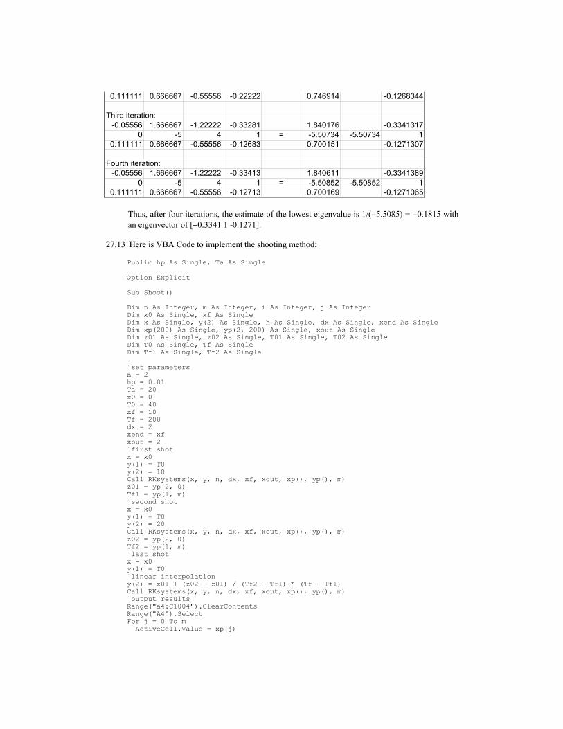
0.111111 0.666667 -0.55556 -0.22222 0.746914 -0.1268344
Third iteration:
-0.05556 1.666667 -1.22222 -0.33281 1.840176 -0.3341317
0 -5 4 1 = -5.50734 -5.50734 1
0.111111 0.666667 -0.55556 -0.12683 0.700151 -0.1271307
Fourth iteration:
-0.05556 1.666667 -1.22222 -0.33413 1.840611 -0.3341389
0 -5 4 1 = -5.50852 -5.50852 1
0.111111 0.666667 -0.55556 -0.12713 0.700169 -0.1271065
Thus, after four iterations, the estimate of the lowest eigenvalue is 1/(−5.5085) = −0.1815 with
an eigenvector of [−0.3341 1 -0.1271].
27.13 Here is VBA Code to implement the shooting method:
Public hp As Single, Ta As Single
Option Explicit
Sub Shoot()
Dim n As Integer, m As Integer, i As Integer, j As IntegerDim x0 As Single, xf As SingleDim x As Single, y(2) As Single, h As Single, dx As Single, xend As SingleDim xp(200) As Single, yp(2, 200) As Single, xout As SingleDim z01 As Single, z02 As Single, T01 As Single, T02 As SingleDim T0 As Single, Tf As SingleDim Tf1 As Single, Tf2 As Single
'set parametersn = 2hp = 0.01Ta = 20x0 = 0T0 = 40xf = 10Tf = 200dx = 2xend = xfxout = 2'first shotx = x0y(1) = T0y(2) = 10Call RKsystems(x, y, n, dx, xf, xout, xp(), yp(), m)z01 = yp(2, 0)Tf1 = yp(1, m)'second shotx = x0y(1) = T0y(2) = 20Call RKsystems(x, y, n, dx, xf, xout, xp(), yp(), m)z02 = yp(2, 0)Tf2 = yp(1, m)'last shotx = x0y(1) = T0'linear interpolationy(2) = z01 + (z02 - z01) / (Tf2 - Tf1) * (Tf - Tf1)Call RKsystems(x, y, n, dx, xf, xout, xp(), yp(), m)'output resultsRange("a4:C1004").ClearContentsRange("A4").SelectFor j = 0 To m ActiveCell.Value = xp(j)
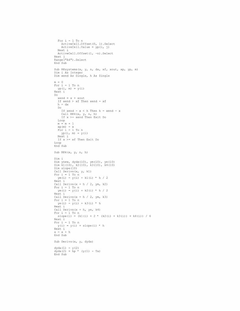
For i = 1 To n ActiveCell.Offset(0, 1).Select ActiveCell.Value = yp(i, j) Next i ActiveCell.Offset(1, -n).SelectNext jRange("A4").SelectEnd Sub
Sub RKsystems(x, y, n, dx, xf, xout, xp, yp, m)Dim i As IntegerDim xend As Single, h As Single
m = 0For i = 1 To n yp(i, m) = y(i)Next iDo xend = x + xout If xend > xf Then xend = xf h = dx Do If xend - x < h Then h = xend - x Call RK4(x, y, n, h) If x >= xend Then Exit Do Loop m = m + 1 xp(m) = x For i = 1 To n yp(i, m) = y(i) Next i If x >= xf Then Exit DoLoopEnd Sub
Sub RK4(x, y, n, h)
Dim iDim ynew, dydx(10), ym(10), ye(10)Dim k1(10), k2(10), k3(10), k4(10)Dim slope(10)Call Derivs(x, y, k1)For i = 1 To n ym(i) = y(i) + k1(i) * h / 2Next iCall Derivs(x + h / 2, ym, k2)For i = 1 To n ym(i) = y(i) + k2(i) * h / 2Next iCall Derivs(x + h / 2, ym, k3)For i = 1 To n ye(i) = y(i) + k3(i) * hNext iCall Derivs(x + h, ye, k4)For i = 1 To n slope(i) = (k1(i) + 2 * (k2(i) + k3(i)) + k4(i)) / 6Next iFor i = 1 To n y(i) = y(i) + slope(i) * hNext ix = x + hEnd Sub
Sub Derivs(x, y, dydx)
dydx(1) = y(2)dydx(2) = hp * (y(1) - Ta)End Sub

27.14
27.15 A general formulation that describes Example 27.3 as well as Probs. 27.3 and 27.5 is
0)(2
2
=+++ xfcydx
dyb
dx
yda
Finite difference approximations can be substituted for the derivatives:
0)(2
2 11
2
11 =++∆
−+
∆
+− −+−+ii
iiiii xfcyx
yyb
x
yyya
Collecting terms
( ) ( ) ( ) 2
1
2
1 )(5.025.0 xxfyxbayxcayxba iiii ∆=∆+−∆++∆−− +−
The following VBA code implants this equation as applied to Example 27.3.

Public hp As Single, dx As SingleOption ExplicitSub FDBoundaryValue()Dim ns As Integer, i As IntegerDim a As Single, b As Single, c As SingleDim e(100) As Single, f(100) As Single, g(100) As SingleDim r(100) As Single, y(100) As SingleDim Lx As Single, xx As Single, x(100) As SingleLx = 10dx = 2ns = Lx / dxxx = 0hp = 0.01a = 1b = 0c = hpy(0) = 40y(ns) = 200For i = 0 To ns x(i) = xx xx = xx + dxNext if(1) = 2 * a / dx ^ 2 + cg(1) = -(a / dx ^ 2 - b / (2 * dx))r(1) = ff(x(1)) + (a / dx ^ 2 + b / (2 * dx)) * y(0)For i = 2 To ns - 2 e(i) = -(a / dx ^ 2 + b / (2 * dx)) f(i) = 2 * a / dx ^ 2 + c g(i) = -(a / dx ^ 2 - b / (2 * dx)) r(i) = ff(x(i))Next ie(ns - 1) = -(a / dx ^ 2 + b / (2 * dx))f(ns - 1) = 2 * a / dx ^ 2 + cr(ns - 1) = ff(x(ns - 1)) + (a / dx ^ 2 - b / (2 * dx)) * y(ns)Sheets("Sheet2").SelectRange("a5:d105").ClearContentsRange("a5").SelectFor i = 1 To ns - 1 ActiveCell.Value = e(i) ActiveCell.Offset(0, 1).Select ActiveCell.Value = f(i) ActiveCell.Offset(0, 1).Select ActiveCell.Value = g(i) ActiveCell.Offset(0, 1).Select ActiveCell.Value = r(i) ActiveCell.Offset(1, -3).SelectNext iRange("a5").SelectCall Tridiag(e, f, g, r, ns - 1, y)Sheets("Sheet1").SelectRange("a5:b105").ClearContentsRange("a5").SelectFor i = 0 To ns ActiveCell.Value = x(i) ActiveCell.Offset(0, 1).Select ActiveCell.Value = y(i) ActiveCell.Offset(1, -1).SelectNext iRange("a5").SelectEnd Sub
Sub Tridiag(e, f, g, r, n, x)Dim k As IntegerFor k = 2 To n e(k) = e(k) / f(k - 1) f(k) = f(k) - e(k) * g(k - 1)Next kFor k = 2 To n r(k) = r(k) - e(k) * r(k - 1)Next kx(n) = r(n) / f(n)
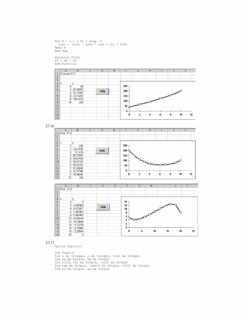
For k = n - 1 To 1 Step -1 x(k) = (r(k) - g(k) * x(k + 1)) / f(k)Next kEnd Sub
Function ff(x)ff = hp * 20End Function
27.16
27.17Option Explicit
Sub Power()Dim n As Integer, i As Integer, iter As IntegerDim aa As Single, bb As SingleDim a(10, 10) As Single, c(10) As SingleDim lam As Single, lamold As Single, v(10) As SingleDim es As Single, ea As Single

es = 0.001n = 3aa = 2 / 0.5625bb = -1 / 0.5625a(1, 1) = aaa(1, 2) = bbFor i = 2 To n - 1 a(i, i - 1) = bb a(i, i) = aa a(i, i + 1) = bbNext ia(i, i - 1) = bba(i, i) = aa
lam = 1For i = 1 To n v(i) = lamNext i
Sheets("sheet1").SelectRange("a3:b1000").ClearContentsRange("a3").SelectDo iter = iter + 1 Call Mmult(a(), (v()), v(), n, n, 1) lam = Abs(v(1)) For i = 2 To n If Abs(v(i)) > lam Then lam = Abs(v(i)) Next i ActiveCell.Value = "iteration: " ActiveCell.Offset(0, 1).Select ActiveCell.Value = iter ActiveCell.Offset(1, -1).Select ActiveCell.Value = "eigenvalue: " ActiveCell.Offset(0, 1).Select ActiveCell.Value = lam ActiveCell.Offset(1, -1).Select For i = 1 To n v(i) = v(i) / lam Next i ActiveCell.Value = "eigenvector:" ActiveCell.Offset(0, 1).Select For i = 1 To n ActiveCell.Value = v(i) ActiveCell.Offset(1, 0).Select Next i ActiveCell.Offset(1, -1).Select ea = Abs((lam - lamold) / lam) * 100 lamold = lam If ea <= es Then Exit DoLoop
End Sub
Sub Mmult(a, b, c, m, n, l)
Dim i As Integer, j As Integer, k As IntegerDim sum As Single
For i = 1 To n sum = 0 For k = 1 To m sum = sum + a(i, k) * b(k) Next k c(i) = sumNext i
End Sub

•••
27.18Option Explicit
Sub Power()Dim n As Integer, i As Integer, iter As Integer, j As IntegerDim aa As Single, bb As SingleDim a(10, 10) As Single, c(10) As SingleDim lam As Single, lamold As Single, v(10) As SingleDim es As Single, ea As SingleDim x(10) As Single, ai(10, 10) As Single
es = 0.0000011n = 3aa = 2 / 0.5625bb = -1 / 0.5625a(1, 1) = aaa(1, 2) = bbFor i = 2 To n - 1 a(i, i - 1) = bb a(i, i) = aa a(i, i + 1) = bbNext ia(i, i - 1) = bba(i, i) = aa
Call LUDminv(a(), n, x())
lam = 1For i = 1 To n v(i) = lamNext i

Sheets("sheet1").SelectRange("a3:j1000").ClearContentsRange("a3").SelectActiveCell.Value = "Matrix inverse:"ActiveCell.Offset(1, 0).SelectFor i = 1 To n For j = 1 To n ActiveCell.Value = a(i, j) ActiveCell.Offset(0, 1).Select Next j ActiveCell.Offset(1, -n).SelectNext iActiveCell.Offset(1, 0).Select
Do iter = iter + 1 Call Mmult(a(), (v()), v(), n, n, 1) lam = Abs(v(1)) For i = 2 To n If Abs(v(i)) > lam Then lam = Abs(v(i)) Next i ActiveCell.Value = "iteration: " ActiveCell.Offset(0, 1).Select ActiveCell.Value = iter ActiveCell.Offset(1, -1).Select ActiveCell.Value = "eigenvalue: " ActiveCell.Offset(0, 1).Select ActiveCell.Value = lam ActiveCell.Offset(1, -1).Select For i = 1 To n v(i) = v(i) / lam Next i ActiveCell.Value = "eigenvector:" ActiveCell.Offset(0, 1).Select For i = 1 To n ActiveCell.Value = v(i) ActiveCell.Offset(1, 0).Select Next i ActiveCell.Offset(1, -1).Select ea = Abs((lam - lamold) / lam) * 100 lamold = lam If ea <= es Then Exit DoLoop
End Sub
Sub Mmult(a, b, c, m, n, l)
Dim i As Integer, j As Integer, k As IntegerDim sum As Single
For i = 1 To n sum = 0 For k = 1 To m sum = sum + a(i, k) * b(k) Next k c(i) = sumNext i
End Sub
Sub LUDminv(a, n, x)Dim i As Integer, j As Integer, er As IntegerDim o(3) As Single, s(3) As Single, b(3) As SingleDim ai(10, 10) As Single, tol As Single
tol = 0.00001Call Decompose(a, n, tol, o(), s(), er)If er = 0 Then For i = 1 To n For j = 1 To n If i = j Then

b(j) = 1 Else b(j) = 0 End If Next j Call Substitute(a, o, n, b, x) For j = 1 To n ai(j, i) = x(j) Next j Next iEnd IfFor i = 1 To n For j = 1 To n a(i, j) = ai(i, j) Next jNext iEnd Sub
Sub Decompose(a, n, tol, o, s, er)Dim i As Integer, j As Integer, k As IntegerDim factor As SingleFor i = 1 To n o(i) = i s(i) = Abs(a(i, 1)) For j = 2 To n If Abs(a(i, j)) > s(i) Then s(i) = Abs(a(i, j)) Next jNext iFor k = 1 To n - 1 Call Pivot(a, o, s, n, k) If Abs(a(o(k), k) / s(o(k))) < tol Then er = -1 Exit For End If For i = k + 1 To n factor = a(o(i), k) / a(o(k), k) a(o(i), k) = factor For j = k + 1 To n a(o(i), j) = a(o(i), j) - factor * a(o(k), j) Next j Next iNext kIf (Abs(a(o(k), k) / s(o(k))) < tol) Then er = -1End Sub
Sub Pivot(a, o, s, n, k)Dim ii As Integer, p As IntegerDim big As Single, dummy As Singlep = kbig = Abs(a(o(k), k) / s(o(k)))For ii = k + 1 To n dummy = Abs(a(o(ii), k) / s(o(ii))) If dummy > big Then big = dummy p = ii End IfNext iidummy = o(p)o(p) = o(k)o(k) = dummyEnd Sub
Sub Substitute(a, o, n, b, x)Dim k As Integer, i As Integer, j As IntegerDim sum As Single, factor As SingleFor k = 1 To n - 1 For i = k + 1 To n factor = a(o(i), k) b(o(i)) = b(o(i)) - factor * b(o(k)) Next iNext kx(n) = b(o(n)) / a(o(n), n)

For i = n - 1 To 1 Step -1 sum = 0 For j = i + 1 To n sum = sum + a(o(i), j) * x(j) Next j x(i) = (b(o(i)) - sum) / a(o(i), i)Next iEnd Sub
•••
27.19 This problem can be solved by recognizing that the solution corresponds to driving thedifferential equation to zero. To do this, a finite difference approximation can be substituted forthe second derivative to give
RT T T
xT Ti i ii i=
− +− × + + −− + −1 1
2
7 4212 10 273 5 150
( ). ( ) ( )
∆
where R = the residual, which is equal to zero when the equation is satisfied. Next, aspreadsheet can be set up as below. Guesses for T can be entered in cells B11:B14. Then, theresidual equation can be written in cells C11:C14 and referenced to the temperatures in columnB. The square of the R’s can then be entered in column D and summed (D17). The Solver canthen be invoked to drive cell D17 to zero by varying B11:B14. The result is as shown in thespreadsheet. A plot is also displayed below.

A B C D
1 E 1
2 sigma 1.20E-07
3 k 5
4 Ta 150
5 T0 200
6 Tn 100
7 dx 0.1
8
9 x T R R^2
10 0 200
11 0.1 133.015 4.32E-05 1.87E-09
12 0.2 97.79076 0.000185 3.42E-08
13 0.3 82.63883 -0.00076 5.8E-07
14 0.4 83.31515 0.001114 1.24E-06
15 0.5 100
16
17 SSR 1.86E-06
=(B10-2*B11+B12)/$B$7^2-$B$2*(B11+273)^4+$B$3*($B$4-B11)
=sum(D11:D14)
0
50
100
150
200
0 0.1 0.2 0.3 0.4 0.5

27.20 First, an m-file containing the system of ODEs can be created and saved (in this case asodesys.m),
function dy = predprey(t,y)dy=[0.3*y(1)-1.5*y(1)*y(2);-0.1*y(2)+0.036*y(1)*y(2)];
Then, the following MATLAB session is used to generate the solution:
>> [t,y]=ode45('odesys',[0 100],[1;.05]);
A plot of the solution along with the state-space plot are generated with
>> plot(t,y)>> plot(y(:,1),y(:,2))
These plots are displayed below
0 20 40 60 80 100
0
2
4
6
8
10
12
14
10
0.5
0
0
27.21 First, the 2nd-order ODE can be reexpressed as the following system of 1st-order ODE’s
dx
dtz
dz
dtz x
=
= − −8 333333 1166 667. .
Next, we create an m-file to hold the ODEs:
function dx=spring(t,y)dx=[y(2);-8.333333*y(2)-1166.667*y(1)]
Then we enter the following commands into MATLAB
[t,y]=ode45('spring',[0 .4],[0.3;0])plot(t,y(:,1));
The following plot results:

0 0.1 0.2 0.3 0.4
-0.4
-0.2
0
0.2
(b) The eigenvalues and eigenvectors can be determined with the following commands:
>> a=[0 -1;8.333333 1166.667];>> format short e>> [v,d]=eig(a)
v =
-9.9997e-001 8.5715e-004 7.1427e-003 -1.0000e+000
d =
7.1429e-003 0 0 1.1667e+003
27.22 This problem is solved in an identical fashion to that employed in Example 27.12. For part (a),the solution is as displayed in the following plot:
0
3
6
0 10 20 30
(b) The solution for this set of equations is laid out in Sec. 28.2 (Fig. 28.9).

27.23


27.24


27.25
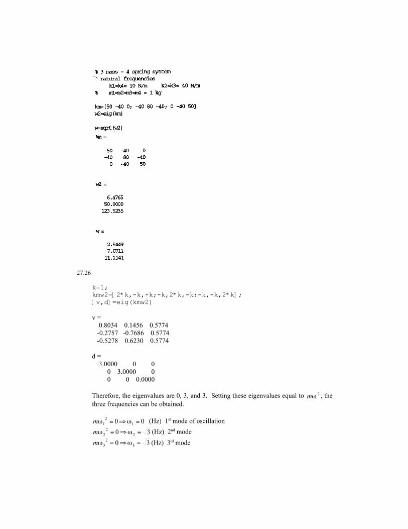
27.26
k=1;kmw2=[2*k,-k,-k;-k,2*k,-k;-k,-k,2*k];[v,d]=eig(kmw2)
v =
0.8034 0.1456 0.5774
-0.2757 -0.7686 0.5774
-0.5278 0.6230 0.5774
d =
3.0000 0 0
0 3.0000 0
0 0 0.0000
Therefore, the eigenvalues are 0, 3, and 3. Setting these eigenvalues equal to 2ωm , the
three frequencies can be obtained.
00 1
2
1 =⇒= ωωm (Hz) 1st mode of oscillation
30 2
2
2 =⇒= ωωm (Hz) 2nd mode
30 3
2
3 =⇒= ωωm (Hz) 3rd mode

27.7 (a) The exact solution is
08.04.025 +++= ttAey t
If the initial condition at t = 0 is 0.8, A = 0,
08.04.02 ++= tty
Note that even though the choice of the initial condition removes the positive exponential terms,it still lurks in the background. Very tiny round off errors in the numerical solutions bring it tothe fore. Hence all of the following solutions eventually diverge from the analytical solution.
(b) 4th order RK. The plot shows the numerical solution (bold line) along with the exact solution(fine line).
-10
-5
0
5
10
15
0 1 2 3 4
(c) function yp=dy(t,y)yp=5*(y-t^2);
>> tspan=[0,5];>> y0=0.08;>> [t,y]=ode45('dy1',tspan,y0);
(d)>> [t,y]=ode23S('dy1',tspan,y0);
(e)>> [t,y]=ode23TB('dy1',tspan,y0);
-30
-20
-10
0
10
20
30
0 1 2 3 4 5
RK4 Analytical ODE45
ODE23S ODE23TP

CHAPTER 29
29.1
First iteration: 7.500000 2.250000 15.675000 9.750000 3.600000 20.782500 55.425000 62.707500 85.047000Error: 100.000000 100.000000 100.000000 100.000000 100.000000 100.000000 100.000000 100.000000 100.000000Second iteration: 9.600000 8.212501 20.563500 26.137500 34.632000 52.916250 68.068500 88.782750 85.500310Error: 21.875000 72.602740 23.772710 62.697270 89.604990 60.725670 18.574660 29.369720 5.301830E-01
•••Seventh iteration: 25.013610 28.806340 33.932440 46.216590 56.257030 56.921290 78.575310 93.082440 87.501180Error: 2.954020E-01 2.531316E-02 1.679560E-02 2.267362E-02 2.082395E-02 1.041445E-02 2.165254E-03 3.590016E-03 1.743838E-03
29.2 The fluxes for Prob. 29.1 can be calculated as
qx= -9.325527E-02 -2.185114E-01 -5.192447E-01 -7.657973E-01 -2.622653E-01 1.532972E-01 -1.668020 -2.186839E-01 1.055520qy= -1.132306 -1.378297 -1.394572 -1.312262 -1.574765 -1.312434 -2.542694 -2.296703 -2.280428qn= 1.136140 1.395511 1.488101 1.519367 1.596454 1.321357 3.040984 2.307091 2.512862theta= -94.708180 -99.008540 -110.421900 -120.266600 -99.455400 -83.337820 -123.265100 -95.439100 -65.162450

29.3 The plate is redrawn below
100 oC
0 oC
75 oC 50 oC
100 oC
0 oC
75 oC 50 oC
After 15 iterations of the Liebmann method, the result is
0 100 100 100 100 100 100 100 0
50 73.6954 82.3973 86.06219 87.7991 88.54443 88.19118 85.32617 75
50 62.3814 69.8296 74.0507 76.58772 78.18341 78.8869 78.10995 75
50 55.9987 60.4898 63.72554 66.32058 68.71677 71.06672 73.23512 75
50 51.1222 52.4078 54.04625 56.25934 59.3027 63.42793 68.75568 75
50 46.0804 43.9764 43.79945 45.37425 48.80563 54.57569 63.33804 75
50 39.2206 33.6217 31.80514 32.62971 35.95756 42.71618 54.995 75
50 27.1773 19.4897 17.16646 17.3681 19.66293 25.31308 38.86852 75
0 0 0 0 0 0 0 0 0
with percent approximate errors of
0 0 0 0 0 0 0 0 0
0 0.0030 0.0040 0.0043 0.0049 0.0070 0.0114 0.0120 0
0 0.0050 0.0062 0.0057 0.0055 0.0079 0.0120 0.0109 0
0 0.0062 0.0067 0.0036 0.0007 0.0007 0.0097 0.0241 0
0 0.0076 0.0066 0.0020 0.0106 0.0067 0.0164 0.0542 0
0 0.0106 0.0079 0.0033 0.0074 0.0077 0.0400 0.1005 0
0 0.0149 0.0099 0.0119 0.0327 0.0630 0.1192 0.2343 0
0 0.0136 0.0013 0.0302 0.1259 0.2194 0.2925 0.7119 0
0 0 0 0 0 0 0 0 0
29.4 The solution is identical to Prob. 29.3, except that now the top edge must be modeled.This means that the nodes along the top edge are simulated with equations of the form
4 2 01 1 1T T T Ti j i j i j i j, , , ,− − − =− + −
The resulting simulation (after 14 iterations) yields
50 50.38683 51.16385 52.6796 55.17802 58.7692 63.41846 68.9398 75
50 50.17211 50.76425 52.15054 54.58934 58.20129 62.96008 68.67918 75
50 49.51849 49.56564 50.58556 52.86931 56.56024 61.64839 67.93951 75
50 48.31607 47.39348 47.78093 49.79691 53.61405 59.2695 66.58047 75
50 46.33449 43.91569 43.37764 44.99165 48.94264 55.38806 64.29121 75
50 43.09381 38.56608 36.8614 37.93565 41.91332 49.21507 60.37012 75
50 37.46764 30.4051 27.61994 28.08718 31.71478 39.39338 53.1291 75
50 26.36368 17.98153 15.18654 15.20479 17.63115 23.73251 38.00928 75
0 0 0 0 0 0 0 0 0
with percent approximate errors of

0 0.0584 0.1318 0.2034 0.2606 0.2828 0.2493 0.1529 0
0 0.0722 0.1603 0.2473 0.3173 0.3424 0.2983 0.1862 0
0 0.0854 0.1883 0.2937 0.3788 0.4077 0.3438 0.2096 0
0 0.0933 0.2121 0.3441 0.4464 0.4754 0.3972 0.2247 0
0 0.0930 0.2300 0.3913 0.5097 0.5328 0.4468 0.2605 0
0 0.0873 0.2469 0.4299 0.5474 0.5611 0.4237 0.2747 0
0 0.0913 0.2827 0.4995 0.5852 0.5525 0.3157 0.0477 0
0 0.1131 0.3612 0.7054 0.9164 0.7958 0.5085 0.6345 0
0 0 0 0 0 0 0 0 0
29.5 The solution is identical to Examples 29.1 and 29.3, except that now heat balancesmust be developed for the three interior nodes on the bottom edge. For example, usingthe control-volume approach, node 1,0 can be modeled as
−−
+−
+−
− =
− − − = −
0 49 510
0 49 510
0 49 1010
2 10 0
4 2 8163265
10 00 20 10 11 10
10 00 20 11
. ( ) . ( ) . ( ) ( )
.
T T T T T T
T T T T
The resulting simulation yields (with a stopping criterion of 1% and a relaxationcoefficient of 1.5)
87.5 100 100 100 75
75 79.91669 77.76103 70.67812 5075 66.88654 60.34068 55.39378 50
75 52.26597 40.84576 40.26148 5075 27.12079 10.54741 14.83802 50
The fluxes for the computed nodes can be computed as
qx
-0.06765 0.226345 0.6801450.359153 0.281573 0.253347
0.836779 0.29411 -0.224281.579088 0.300928 -0.96659
qy-0.81128 -0.97165 -1.09285
-0.67744 -0.90442 -0.74521-0.97426 -1.21994 -0.99362
-1.23211 -1.48462 -1.24575
qn
0.814095 0.997668 1.2872160.766759 0.947241 0.787095
1.284283 1.254887 1.0186142.002904 1.514811 1.576764
θ (radians)
-1.65398 -1.34193 -1.0141
-1.08331 -1.26898 -1.24309-0.86117 -1.33422 -1.7928

-0.66259 -1.37081 -2.23067
θ (degrees)
-94.7663 -76.8869 -58.1036
-62.0692 -72.7072 -71.2236-49.3412 -76.4454 -102.72
-37.9638 -78.5416 -127.808
29.6 The solution is identical to Example 29.5 and 29.3, except that now heat balances mustbe developed for the interior nodes at the lower left and the upper right edges. Thebalances for nodes 1,1 and 3,3 can be written as
− + + = − +
− + + = − +
4 08453 0 8453 1154701
4 0 8453 0 8453 1154701
11 21 12 01 10
33 32 23 34 43
T T T T T
T T T T T
. . . ( )
. . . ( )
Using the appropriate boundary conditions, simple Laplacians can be used for theremaining interior nodes. The resulting simulation yields
75 50 50 50
100 75 63.97683 55.90731 50
100 86.02317 75 63.97683 50
100 94.09269 86.02317 75 50
100 100 100 75
29.7 The nodes to be simulated are
0,0 1,0 2,0 3,0
0,1 1,1 2,1 3,1
0,2 1,2 2,2 3,2
0,3 1,3 2,3 3,3
0,0 1,0 2,0 3,0
0,1 1,1 2,1 3,1
0,2 1,2 2,2 3,2
0,3 1,3 2,3 3,3
Simple Laplacians are used for all interior nodes. Balances for the edges must takeinsulation into account. Fo example, node 1,0 is modeled as
4 2 01 0 0 0 2 0 1 1T T T T, , , ,− − − =
The corner node, 0,0 would be modeled as
4 2 2 00 0 1 0 0 1T T T, , ,− − =

The resulting set of equations can be solved for
0 12.5 25 37.5 50
11.94853 16.08456 22.79412 30.14706 37.5
15.625 17.09559 19.94485 22.79412 25
16.36029 16.72794 17.09559 16.08456 12.5
16.36029 16.36029 15.625 11.94853 0
The fluxes can be computed as
Jx-0.6125 -0.6125 -0.6125 -0.6125 -0.6125
-0.20267 -0.26572 -0.34453 -0.36029 -0.36029
-0.07206 -0.10584 -0.13961 -0.12385 -0.10809
-0.01801 -0.01801 0.015763 0.112592 0.175643
-5.6E-13 0.018015 0.108088 0.382812 0.585478
Jy0.585478 0.175643 -0.10809 -0.36029 -0.6125
0.382812 0.112592 -0.12385 -0.36029 -0.6125
0.108088 0.015763 -0.13961 -0.34453 -0.6125
0.018015 -0.01801 -0.10584 -0.26572 -0.6125
0 -0.01801 -0.07206 -0.20267 -0.6125
Jn0.847314 0.637187 0.621964 0.710611 0.866206
0.43315 0.288587 0.366116 0.509533 0.710611
0.129906 0.107004 0.197444 0.366116 0.621964
0.025477 0.025477 0.107004 0.288587 0.637187
5.63E-13 0.025477 0.129906 0.43315 0.847314
θ (radians)2.378747 2.862322 -2.96692 -2.60987 -2.35619
2.057696 2.740799 -2.7965 -2.35619 -2.10252
2.158799 2.993743 -2.35619 -1.91589 -1.74547
2.356194 -2.35619 -1.42295 -1.17 -1.29153
3.141593 -0.7854 -0.588 -0.4869 -0.80795
θ (degrees)136.2922 163.999 -169.992 -149.534 -135
117.8973 157.0362 -160.228 -135 -120.466
123.6901 171.5289 -135 -109.772 -100.008
135 -135 -81.5289 -67.0362 -73.999
180 -45 -33.6901 -27.8973 -46.2922

29.8 Node 0,3:
There are two approaches for modeling this node. One would be to consider it a Dirichlet nodeand not model it at all (i.e., set it’s temperature at 50oC). The second alternative is to use a heatbalance to model it as shown here
(0,3) (1,3)
(0,2)
(0,3) (1,3)
(0,2)
0 05 15 140
0 5 20 130
0 01 20 1 101 3 0 3 0 3 0 2
0 3=−
−−
+ −. ( )( ) . ( )( ) . ( )( )( ), , , ,
,
T T T TT
− + − =0 29752 4 0 52893 3173551 3 0 3 0 2. . ., , ,T T T
Node 2,3:
0 0 5 15 140
0 5 15 120
0 5 30 130
0 01 30 1 102 3 1 3 3,3 2 3 2 3 2 2
2 3= −−
+−
−−
+ −. ( )( ) . ( )( ) . ( )( ) . ( )( )( ), , , , ,
,
T T T T T TT
4 0 70588 141176 1882352 3 1 3 3,3 2 2T T T T, , ,. . .− − −
Node 2,2:
(1,2)
(2,3)
(2,2)
(3,2)
(2,1)
(1,2)
(2,3)
(2,2)
(3,2)
(2,1)
0 0 5 22 5 140
05 22 5 120
05 30 115
05 30 130
10 7 5
2 2 1 2 3,2 2 2 2 2 2 1
2 3 2 2 2
= −−
+−
−−
+−
+
. ( . )( ) . ( . )( ) . ( )( )
. ( )( ) ( . )
, , , , ,
, ,
T T T T T T
T T π
4 0 48 0 96 170667 085333 3015 932 2 1 2 3,2 2 1 2 3T T T T T, , , ,. . . . .− − − − =

Node 5,3:
(4,3) (5,3)
(5,2)
0 0 5 15 120
05 10 130
0 01 10 1 105,3 4 3 5,3 5,2
5,3= −−
−−
+ −. ( )( ) . ( )( ) . ( )( )( ),T T T T
T
4 2 33766 103896 6 233775,3 4 3 5,2T T T− − =. . .,
29.9 Node 0,0:
(0,1)
(1,0)
(0,0)
0 0 01 7 5 2 20 0 7 7 5 240
0 7 20 215
0 0
1 0 0 0 0 1 0 0= − −−
+−
. ( . )( )( ) . ( . )( ) . ( )( ),
, , , ,T
T T T T
4 0 46069 3 27605 5 265080 0 1 0 0 1T T T, , ,. . .− − =
Node 1,1:
(0,1)
(1,2)
(1,1)
(2,1)
(1,0)
0 0 7 22 5 240
05 22 5 220
0 7 20 215
0 5 10 215
0 7 20 230
05 10 230
1 1 0 1 2 1 1 1 1 1 1 0
1 1 1 0 1 2 1 1 1 2 1 1
= −−
+−
−−
−− − −
. ( . )( ) . ( . )( ) . ( )( )
. ( )( ) . ( )( ) . ( )( )
, , , , , ,
, , , , , ,
T T T T T T
T T T T T T + +
4 0 78755 177389 0 88694 055142 01 1 2 1 1 0 1 2 0 1T T T T T, , , , ,. . . .− − − − =
Node 2,1:

(1,1)
(2,2)
(2,1)
(3,1)
(2,0)
0 0 5 22 5 220
0 5 22 5 220
0 5 20 215
05 20 230
10 22 5 20
2 1 1 1 3,1 2 1 2 1 2 0
2 2 2 1
= −−
+−
−−
−−
+
. ( . )( ) . ( . )( ) . ( )( )
. ( )( ) ( . )( )
, , , , ,
, ,
T T T T T T
T T
4 105882 105882 12549 0 62745 4235 292 1 1 1 3,1 2 0 2 2T T T T T, , , ,. . . . .− − − − =
29.10 The control volume is drawn as in
0, j+1
0, j-1
1, j
A flux balance around the node can be written as (note ∆x = ∆y = h)
−−
+−
−−
=−kh z
T T
hk h z
T T
hk h z
T T
h
j j j j j j∆ ∆ ∆1 0 0 0 1 1 02 2 0
, , , , , ,( / ) ( / )
Collecting and cancelling terms gices
T T T Tj j j j0 0 1 0 1 12 0, , , ,− − − =− +
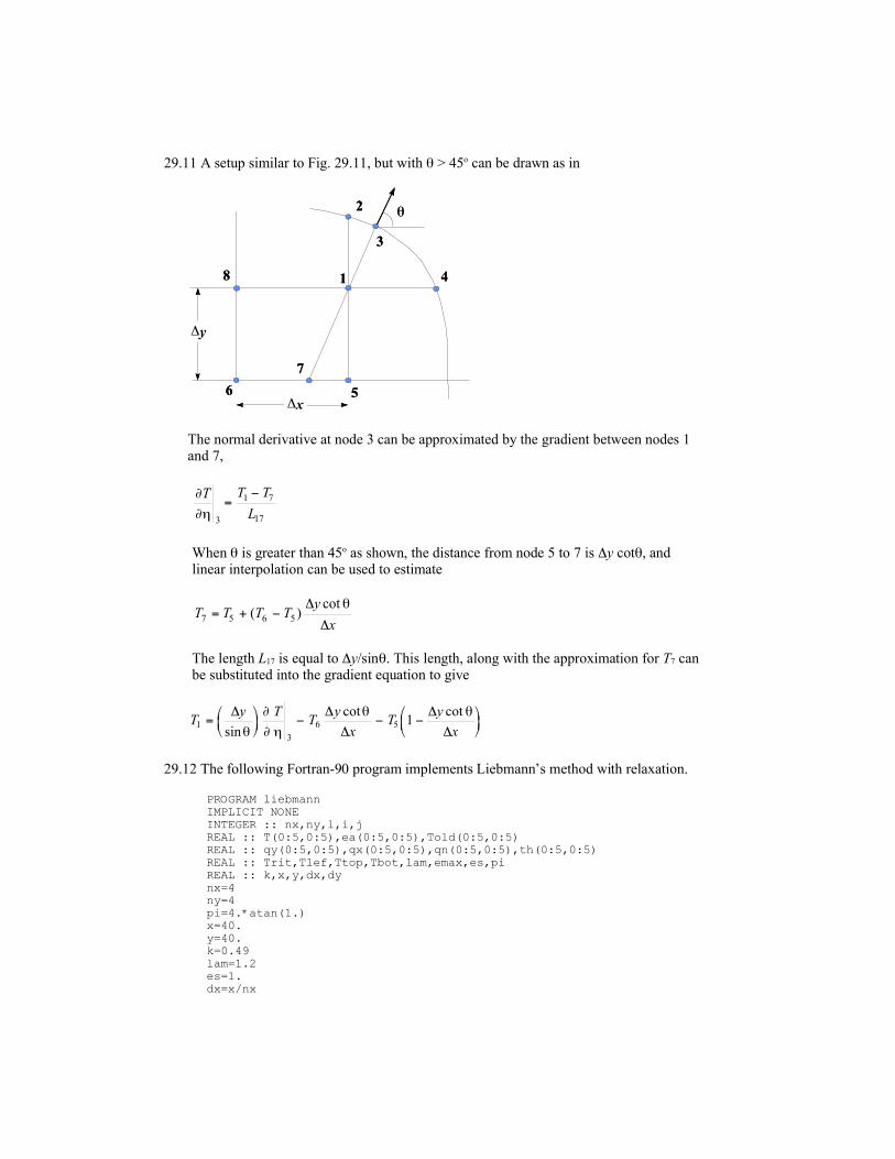
29.11 A setup similar to Fig. 29.11, but with θ > 45o can be drawn as in
θ
1
2
3
4
56
7
∆y
∆x
8
θ
1
2
3
4
56
7
∆y
∆x
8
The normal derivative at node 3 can be approximated by the gradient between nodes 1and 7,
∂
∂η
T T T
L3
1 7
17
=−
When θ is greater than 45o as shown, the distance from node 5 to 7 is ∆y cotθ, andlinear interpolation can be used to estimate
T T T Ty
x7 5 6 5= + −( )
cot∆
∆
θ
The length L17 is equal to ∆y/sinθ. This length, along with the approximation for T7 canbe substituted into the gradient equation to give
Ty T
Ty
xT
y
x1
3
6 5 1=
− − −
∆ ∆
∆
∆
∆sin
cot cot
θ
∂
∂ η
θ θ
29.12 The following Fortran-90 program implements Liebmann’s method with relaxation.
PROGRAM liebmann IMPLICIT NONE INTEGER :: nx,ny,l,i,j REAL :: T(0:5,0:5),ea(0:5,0:5),Told(0:5,0:5) REAL :: qy(0:5,0:5),qx(0:5,0:5),qn(0:5,0:5),th(0:5,0:5) REAL :: Trit,Tlef,Ttop,Tbot,lam,emax,es,pi REAL :: k,x,y,dx,dy nx=4 ny=4 pi=4.*atan(1.) x=40. y=40. k=0.49 lam=1.2 es=1. dx=x/nx

dy=y/ny Tbot=0. Tlef=25. Trit=50. Ttop=150. DO i=1,nx-1 T(i,0)=Tbot END DO DO i=1,nx-1 T(i,ny)=Ttop END DO DO j=1,ny-1 T(0,j)=Tlef END DO DO j=1,ny-1 T(nx,j)=Trit END DO l=0 DO l=l+1 emax=0. DO j = 1,ny-1 DO i = 1,nx-1 Told(i,j)=T(i,j) T(i,j)=(T(i+1,j)+T(i-1,j)+T(i,j+1)+T(i,j-1))/4 T(i,j)=lam*T(i,j)+(1-lam)*Told(i,j) ea(i,j)=abs((T(i,j)-Told(i,j))/T(i,j))*100. if(ea(i,j).GT.emax) emax=ea(i,j) END DO END DO PRINT *, 'iteration = ',l DO j = 1,ny-1 PRINT *, (T(i,j),i=1,nx-1) END DO PRINT * DO j = 1,ny-1 PRINT *, (ea(i,j),i=1,nx-1) END DO IF (emax.LE.es) EXIT END DO DO j = 1,ny-1 DO i = 1,nx-1 qy(i,j)=-k*(T(i,j+1)-T(i,j-1))/2/dy qx(i,j)=-k*(T(i+1,j)-T(i-1,j))/2/dx qn(i,j)=sqrt(qy(i,j)**2+qx(i,j)**2) th(i,j)=atan2(qy(i,j),qx(i,j))*180./pi END DO END DO PRINT *,'qx=' DO j = 1,ny-1 PRINT *, (qx(i,j),i=1,nx-1) END DO PRINT *,'qy=' DO j = 1,ny-1 PRINT *, (qy(i,j),i=1,nx-1) END DO PRINT *,'qn=' DO j = 1,ny-1 PRINT *, (qn(i,j),i=1,nx-1) END DO PRINT *,'theta=' DO j = 1,ny-1 PRINT *, (th(i,j),i=1,nx-1) END DO END

When the program is run, the result of the last iteration is:
iteration = 6 42.81303 33.26489 33.93646 63.17175 56.26600 52.46138 78.57594 76.12081 69.64268
0.5462000 0.1074174 2.4864437E-02 1.1274090E-02 2.0983342E-02 4.8064217E-02 3.1769749E-02 3.6572997E-02 2.4659829E-02 qx= 1.022510 0.2174759 -0.4100102 0.4589829 0.2624041 0.1535171 -2.7459882E-02 0.2188648 0.6399599 qy= -1.547708 -1.378517 -1.285304 -0.8761914 -1.049970 -0.8748025 -0.9022922 -1.071483 -1.164696 qn= 1.854974 1.395566 1.349116 0.9891292 1.082263 0.8881705 0.9027100 1.093608 1.328934 theta= -56.54881 -81.03486 -107.6926 -62.35271 -75.96829 -80.04664 -91.74317 -78.45538 -61.21275Press any key to continue
29.13 When the program is run, the result of the last iteration is:
iteration = 7 25.01361 28.80634 33.93244 46.21659 56.25703 56.92129 78.57531 93.08244 87.50118
0.2954020 2.5313158E-02 1.6795604E-02 2.2673620E-02 2.0823948E-02 1.0414450E-02 2.1652540E-03 3.5900162E-03 1.7438381E-03 qx= -9.3255267E-02 -0.2185114 -0.5192447 -0.7657973 -0.2622653 0.1532972 -1.668020 -0.2186839 1.055520 qy= -1.132306 -1.378297 -1.394572 -1.312262 -1.574765 -1.312434 -2.542694 -2.296703 -2.280428 qn= 1.136140 1.395511 1.488101 1.519367 1.596454 1.321357 3.040984 2.307091 2.512862 theta= -94.70818 -99.00854 -110.4219 -120.2666 -99.45540 -83.33782 -123.2651 -95.43910 -65.16245Press any key to continue
29.14 When the program is run, the result of the last iteration is:
iteration = 1938.490 24.764 19.044 16.783 16.696 19.176 27.02854.430 41.832 34.955 31.682 31.041 33.110 38.97662.710 53.570 47.660 44.291 42.924 43.388 45.79968.165 62.478 58.219 55.234 53.215 51.848 50.85472.761 70.301 67.841 65.489 63.051 60.034 55.780

77.795 78.373 77.594 76.027 73.595 69.522 62.23385.175 87.944 88.261 87.530 85.843 82.249 73.624
This data can be imported into Excel and the following contour plot created:
0 5 10 15 20 25 30 35 40
0
5
10
15
20
25
30
35
40
80-100
60-80
40-60
20-40
0-20

29.15

29.16

CHAPTER 30
30.1 The key to approaching this problem is to recast the PDE as a system of ODEs. Thus, bysubstituting the finite-difference approximation for the spatial derivative, we arrive atthe following general equation for each node
dT
dtk
T T T
x
i i i i=− +− +1 1
2
2
∆
By writing this equation for each node, the solution reduces to solving 4 simultaneousODEs with Heun’s method. The results for the first two steps along with some laterselected values are tabulated below. In addition, a plot similar to Fig. 30.4, is also shown
t x = 0 x = 2 x = 4 x = 6 x = 8 x = 10
0 100 0 0 0 0 50
0.1 100 2.04392 0.02179 0.01089 1.02196 50
0.2 100 4.00518 0.08402 0.04267 2.00259 50
•••3 100 37.54054 10.2745 6.442321 18.95732 50
6 100 53.24295 24.66054 17.46032 27.92252 50
9 100 62.39033 36.64937 27.84901 34.34692 50
12 100 68.71329 46.03496 36.5421 39.53549 50
0
20
40
60
80
100
0 5 10
t = 0
t = 3
t = 6
t = 9
t = 12
30.2 Because we now have derivative boundary conditions, the boundary nodes must besimulated. For node 0,
T T T T Tl l l l l
01
0 1 0 12+
−= + − +λ( ) (i)
This introduces an exterior node into the solution at i = −1. The derivative boundarycondition can be used to eliminate this node,
dT
dx
T T
x0
1 1
2=
− −
∆
which can be solved for
dx
dTxTT 0
11 2∆−=−
which can be substituted into Eq. (i) to give

∆−−+=+
dx
dTxTTTT
lllll 0
0101
0 222λ
For our case, dT0/dx = 1 and ∆x = 2, and therefore T−1 = T1 + 4. This can be substitutedinto Eq. (i) to give,
)422( 0101
0 +−+=+ llll TTTT λ
A similar analysis can be used to embed the zero derivative in the equation for the fifthnode. The result is
T T T Tl l l l
51
5 4 52 2+ = + −λ( )
Together with the equations for the interior nodes, the entire system can be iterated witha step of 0.1 s. The results for some of the early steps along with some later selectedvalues are tabulated below. In addition, a plot of the later results is also shown
t x = 0 x = 2 x = 4 x = 6 x = 8 x = 10
0 50.0000 50.0000 50.0000 50.0000 50.0000 50.0000
0.1 49.9165 50.0000 50.0000 50.0000 50.0000 49.9165
0.2 49.8365 49.9983 50.0000 50.0000 49.9983 49.8365
0.3 49.7597 49.9949 50.0000 50.0000 49.9949 49.7597
0.4 49.6861 49.9901 49.9999 49.9999 49.9901 49.6861
0.5 49.6153 49.9840 49.9997 49.9997 49.9840 49.6153
•••
200 30.00022 31.80019 33.20009 34.19992 34.79981 34.99978
400 13.30043 15.10041 16.50035 17.50028 18.10024 18.30023
600 -3.40115 -1.60115 -0.20115 0.798846 1.398847 1.598847
800 -20.1055 -18.3055 -16.9055 -15.9055 -15.3055 -15.1055
1000 -36.8103 -35.0103 -33.6103 -32.6103 -32.0103 -31.8103
-40
-20
0
20
40
0 2 4 6 8 10
0
200
400
600
800
1000
Notice what’s happening. The rod never reaches a steady state, because of the heat lossat the left end (unit gradient) and the insulated condition (zero gradient) at the right.
30.3 The solution for ∆t = 0.1 is (as computed in Example 30.1),

t x = 0 x = 2 x = 4 x = 6 x = 8 x = 10
0 100 0 0 0 0 50
0.1 100 2.0875 0 0 1.04375 50
0.2 100 4.087847 0.043577 0.021788 2.043923 50
For ∆t = 0.05, it is
t x = 0 x = 2 x = 4 x = 6 x = 8 x = 10
0 100 0 0 0 0 50
0.05 100 1.04375 0 0 0.521875 50
0.1 100 2.065712 1.09E-02 5.45E-03 1.032856 50
0.15 100 3.066454 3.23E-02 0.016228 1.533227 50
0.2 100 4.046528 6.38E-02 3.22E-02 2.023265 50
To assess the differences between the results, we performed the simulation a third time
using a more accurate approach (the Heun method) with a much smaller step size (∆t =0.001). It was assumed that this more refined approach would yield a prediction close totrue solution. These values could then be used to assess the relative errors of the twoEuler solutions. The results are summarized as
x = 0 x = 2 x = 4 x = 6 x = 8 x = 10
Heun (h = 0.001) 100 4.006588 0.083044 0.042377 2.003302 50
Euler (h = 0.1) 100 4.087847 0.043577 0.021788 2.043923 50
Error relative to Heun 2.0% 47.5% 48.6% 2.0%
Euler (h = 0.05) 100 4.046528 0.063786 0.032229 2.023265 50
Error relative to Heun 1.0% 23.2% 23.9% 1.0%
Notice, that as would be expected for Euler’s method, halving the step sizeapproximately halves the global relative error.
30.4 The approach described in Example 30.2 must be modified to account for the zeroderivative at the right hand node (i = 5). To do this, Eq. (30.8) is first written for thatnode as
− + + − =+ + +λ λ λT T T Tl l l l
41
51
61
51 2( ) (i)
The value outside the system (i = 6) can be eliminated by writing the finite differencerelationship for the derivative at node 5 as
dT
dx
T T
x5
6 4
2=
−
∆
which can be solved for
T T xdT
dx6 4
5
2= − ∆
For our case, dT/dx = 0, so T6 = T4 and Eq. (i) becomes

− + + =+ +2 1 24
15
15λ λT T T
l l l( )
Thus, the simultaneous equations to be solved at the first step are
1 04175 0 020875
0 020875 1 04175 0 020875
0 020875 1 04175 0 020875
0 020875 1 04175 0 020875
0 04175 1 04175
2 0875
0
0
0
0
11
21
31
41
51
. .
. . .
. . .
. . .
. .
.−
− −
− −
− −
−
=
T
T
T
T
T
which can be solved for
2 004645
0 040186
0 000806
162 10
6 47 10
5
7
.
.
.
.
.
×
×
−
−
For the second step, the right-hand side is modified to reflect these computed values ofT at t = 0.1,
1 04175 0 020875
0 020875 1 04175 0 020875
0 020875 1 04175 0 020875
0 020875 1 04175 0 020875
0 04175 1 04175
4 092145
0 040186
0 000806
162 10
6 47 10
11
21
31
41
51
5
7
. .
. . .
. . .
. . .
. .
.
.
.
.
.
−
− −
− −
− −
−
=
×
×
−
−
T
T
T
T
T
which can be solved for
3930497
0117399
0 003127
7 83 10
3 76 10
5
6
.
.
.
.
.
×
×
−
−
30.5 The solution is identical to Example 30.3, but with 6 segments. Thus, the simultaneousequations to be solved at the first step are
2 06012 0 03006
0 020875 2 06012 0 03006
0 03006 2 06012 0 03006
0 03006 2 06012 0 03006
0 03006 2 06012
6 012
0
0
0
3 006
11
21
31
41
51
. .
. . .
. . .
. . .
. .
.
.
−
− −
− −
− −
−
=
T
T
T
T
T
which can be solved for

2 91890
0 04260
0 00093
0 02131
145945
.
.
.
.
.
For the second step, the right-hand side is modified to reflect these computed values ofT at t = 0.1,
2 06012 0 03006
0 020875 2 06012 0 03006
0 03006 2 06012 0 03006
0 03006 2 06012 0 03006
0 03006 2 06012
1167559
017042
0 00373
0 08524
583780
11
21
31
41
51
. .
. . .
. . .
. . .
. .
.
.
.
.
.
−
− −
− −
− −
−
=
T
T
T
T
T
which can be solved for
5 66986
016553
0 00543
0 08282
2 83493
.
.
.
.
.
The solution at t = 10 for this problem (n = 6) along with the results determined for n =5, as in Example 30.3, are displayed in the following plot:
0
50
100
0 5 10
30.6 Using the approach followed in Example 30.5, Eq. (30.20) is applied to nodes (1,1),(1,2), and (1,3) to yield the following tridiagonal equations
2 167 0 0835
0 0835 2 167 0 0835
0 0835 2167
6 2625
6 2625
18 7875
1 1
1 2
1 3
. .
. . .
. .
.
.
.
,
,
,
−
− −
−
=
T
T
T
which can be solved for
T T T1 1 1 2 1 33 018843 3 345301 8 798722, , ,. . .= = =

In a similar fashion, tridiagonal equations can be developed and solved for
T T T2 1 2 2 2 30130591 0 370262 6133184, , ,. . .= = =
and
T T T3,1 3,2 3,311017962 1287655 7 029137= = =. . .
For the second step to t = 10, Eq. (30.22) is applied to nodes (1,1), (2,1), and (3,1) toyield
2 167 0 0835
0 0835 2 167 0 0835
0 0835 2167
12 07537
0 27029
4 060943
1 1
1 2
1 3
. .
. . .
. .
.
.
.
,
,
,
−
− −
−
=
T
T
T
which can be solved for
T T T1 1 1 2 1 355883 0 412884 1889903, , ,. . .= = =
Tridiagonal equations for the other rows can be developed and solved for
T T T2 1 2 2 2 36 308761 0 902193 2 430939, , ,. . .= = =
and
T T T3,1 3,2 3,316 8241 12 1614 1325121= = =. . .
Thus, the result at the end of the first step can be summarized as
i = 0 i = 1 i = 2 i = 3 i = 4j = 4 150 150 150j = 3 75 16.824 12.161 13.251 25j = 2 75 6.309 0.902 2.431 25j = 1 75 5.588 0.413 1.89 25j = 0 0 0 0
The computation can be repeated, and the results for t = 2000 s are below:
i = 0 i = 1 i = 2 i = 3 i = 4j = 4 150 150 150j = 3 75 98.214 97.768 80.357 25j = 2 75 70.089 62.5 48.661 25j = 1 75 44.643 33.482 26.786 25j = 0 0 0 0
30.7 Although this problem can be modeled with the finite-difference approach (see Sec.32.1), the control-volume method provides a more straightforward way to handle theboundary conditions.
The boundary fluxes and the reaction term can be used to develop the discrete form ofthe advection-diffusion equation for the interior volumes as

∆∆ ∆
∆xdc
dtD
c c
xD
c c
xU
c cU
c ck xci
lil
il
il
il
il
il
il
il
il= −
−+
−+
+−
+−− + − +1 1 1 1
2 2
or dividing both sides by ∆x,
dc
dtD
c c c
xU
c c
xkci
lil
il
il
il
il
il=
− +−
+−+ − + −1 1
2
1 12
2∆ ∆
which is precisely the form that would have resulted by substituting centered finitedifference approximations into the advection-diffusion equation.
For the first boundary node, no diffusion is allowed up the entrance pipe and advectionis handled with a backward difference,
∆∆
∆xdc
dtD
c c
xUc U
c ck xc
l l ll
l ll1 2 1
02 1
12
=−
+ −+
−
or dividing both sides by ∆x,
dc
dtD
c c
x
c c c
xkc
l l l l l ll1 2 1
2
0 2 11
2
2=
−+
− −−
∆ ∆
For the last boundary node, no diffusion is allowed through the exit pipe and advectionout of the tank is again handled with a backward difference,
∆∆
∆xdc
dtD
c c
xU
c cUc k xcn
lnl
nl
nl
nl
nl
nl= −
−+
+− −− −1 1
2
or dividing both sides by ∆x,
dc
dtD
c c
xU
c c
xkcn
lnl
nl
nl
nl
nl= −
−+
−−− −1
2
1
2∆ ∆
By writing these equations for each equally-spaced volume, the PDE is transformed intoa system of ODEs. Explicit methods like Euler’s method or other higher-order RKmethods can then be used to solve the system.
The results with and initial condition that the reactor has zero concentration with aninflow concentration of 100 (using Euler with a step size of 0.005) for t = 100 are
x 0.5 1.5 2.5 3.5 4.5 5.5 6.5 7.5 8.5 9.5
c 14.2042 12.6506 11.2610 10.0385 8.9847 8.1025 7.3928 6.8583 6.5000 6.3201
The results are also plotted below:

0
4
8
12
16
0 2 4 6 8 10
30.8Option Explicit
Sub EulerPDE()
Dim i As Integer, j As Integer, np As Integer, ns As IntegerDim Te(20) As Single, dTe(20) As Single, tpr(20) As Single, Tepr(20, 20)As SingleDim k As Single, dx As Single, L As Single, tc As Single, tf As SingleDim tp As Single, t As Single, tend As Single, h As Single
L = 10ns = 5dx = 2k = 0.835Te(0) = 100Te(5) = 50tc = 0.1tf = 1tp = 0.1np = 0tpr(np) = tFor i = 0 To ns Tepr(i, np) = Te(i)Next iDo tend = t + tp If tend > tf Then tend = tf h = tc Do If t + h > tend Then h = tend - t Call Derivs(Te, dTe, ns, dx, k) For j = 1 To ns - 1 Te(j) = Te(j) + dTe(j) * h Next j t = t + h If t >= tend Then Exit Do Loop np = np + 1 tpr(np) = t For j = 0 To ns Tepr(j, np) = Te(j) Next j If t >= tf Then Exit DoLoopSheets("sheet1").SelectRange("a4").SelectFor i = 0 To np ActiveCell.Value = tpr(i) For j = 0 To ns ActiveCell.Offset(0, 1).Select ActiveCell.Value = Tepr(j, i) Next j

ActiveCell.Offset(1, -ns - 1).SelectNext i
End Sub
Sub Derivs(Te, dTe, ns, dx, k)
Dim j As IntegerFor j = 1 To ns - 1 dTe(j) = k * (Te(j - 1) - 2 * Te(j) + Te(j + 1)) / dx ^ 2Next jEnd Sub
30.9 This program is set up to either use Dirichlet or gradient boundary conditions dependingon the values of the parameters istrt and iend.
Option Explicit
Sub EulerPDE()
Dim i As Integer, j As Integer, np As Integer, ns As IntegerDim istrt As Integer, iend As IntegerDim Te(20) As Single, dTe(20) As Single, tpr(200) As Single, Tepr(20,200) As SingleDim k As Single, dx As Single, L As Single, tc As Single, tf As SingleDim tp As Single, t As Single, tend As Single, h As SingleDim dTedx(20) As Single
L = 10ns = 5dx = 2k = 0.835dTedx(0) = 1istrt = 0dTedx(ns) = 0iend = nsTe(0) = 50Te(1) = 50Te(2) = 50Te(3) = 50Te(4) = 50Te(5) = 50tc = 0.1tf = 1000tp = 200np = 0tpr(np) = tFor i = 0 To ns Tepr(i, np) = Te(i)Next i
Do tend = t + tp If tend > tf Then tend = tf h = tc Do If t + h > tend Then h = tend - t Call Derivs(Te(), dTe(), istrt, iend, ns, dx, k, dTedx()) For j = istrt To iend Te(j) = Te(j) + dTe(j) * h
Next j t = t + h If t >= tend Then Exit Do Loop np = np + 1 tpr(np) = t For j = 0 To ns Tepr(j, np) = Te(j) Next j If t >= tf Then Exit DoLoop

Sheets("sheet1").SelectRange("a4").SelectFor i = 0 To np ActiveCell.Value = tpr(i) For j = 0 To ns ActiveCell.Offset(0, 1).Select ActiveCell.Value = Tepr(j, i) Next j ActiveCell.Offset(1, -ns - 1).SelectNext i
End Sub
Sub Derivs(Te, dTe, istrt, iend, ns, dx, k, dTedx)
Dim j As IntegerIf istrt = 0 Then dTe(0) = k * (2 * Te(1) - 2 * Te(0) - 2 * dx * dTedx(0)) / dx ^ 2End IfFor j = 1 To ns - 1 dTe(j) = k * (Te(j - 1) - 2 * Te(j) + Te(j + 1)) / dx ^ 2Next jIf iend = ns Then dTe(ns) = k * (2 * Te(ns - 1) - 2 * Te(ns) + 2 * dx * dTedx(ns)) / dx^ 2End If
End Sub
30.10
Option Explicit
Sub SimpImplicit()
Dim np, ns, i, j, nDim Te(10), dTe(10), tpr(100), Tepr(10, 100), Tei As SingleDim k, dx, L, tc, tf, tp, t, tend, h, lambdaDim e(10), f(10), g(10), r(10), x(10), xrod
L = 10#ns = 5dx = L / nsk = 0.835Te(0) = 100#Te(ns) = 50#Tei = 0For i = 1 To ns - 1 Te(i) = TeiNext it = 0np = 0tpr(np) = tFor i = 0 To ns Tepr(i, np) = Te(i)Next itc = 0.1tp = 0.1tf = 1
Do tend = t + tp If tend > tf Then tend = tf h = tc Do If t + h > tend Then h = tend - t lambda = k * h / dx ^ 2 f(1) = 1 + 2 * lambda g(1) = -lambda r(1) = Te(1) + lambda * Te(0) For j = 2 To ns - 2 e(j) = -lambda

f(j) = 1 + 2 * lambda g(j) = -lambda r(j) = Te(j) Next j e(ns - 1) = -lambda f(ns - 1) = 1 + 2 * lambda r(ns - 1) = Te(ns - 1) + lambda * Te(ns) Call Tridiag(e(), f(), g(), r(), Te(), ns - 1) t = t + h If t >= tend Then Exit Do Loop np = np + 1 tpr(np) = t For j = 0 To ns Tepr(j, np) = Te(j) Next j If t >= tf Then Exit DoLoop
Range("b5").Selectxrod = 0For j = 0 To ns ActiveCell.Value = xrod ActiveCell.Offset(0, 1).Select xrod = xrod + dxNext jRange("a6").SelectFor i = 0 To np ActiveCell.Value = "t = " & tpr(i) For j = 0 To ns ActiveCell.Offset(0, 1).Select ActiveCell.Value = Tepr(j, i) Next j ActiveCell.Offset(1, -ns - 1).SelectNext iRange("a6").Select
End Sub
Sub Tridiag(e, f, g, r, x, n)
Call Decomp(e, f, g, n)Call Substit(e, f, g, r, n, x)
End Sub
Sub Decomp(e, f, g, n)
Dim k As IntegerFor k = 2 To n e(k) = e(k) / f(k - 1) f(k) = f(k) - e(k) * g(k - 1)Next kEnd Sub
Sub Substit(e, f, g, r, n, x)
Dim k As IntegerFor k = 2 To n r(k) = r(k) - e(k) * r(k - 1)Next kx(n) = r(n) / f(n)For k = n - 1 To 1 Step -1 x(k) = (r(k) - g(k) * x(k + 1)) / f(k)Next kEnd Sub
30.11
Option Explicit

Sub CrankNic()
Dim np, ns, i, j, nDim Te(10), dTe(10), tpr(100), Tepr(10, 100), Tei As SingleDim k, dx, L, tc, tf, tp, t, tend, h, lambdaDim e(10), f(10), g(10), r(10), x(10), xrod
L = 10#ns = 5dx = L / nsk = 0.835Te(0) = 100#Te(5) = 50#Tei = 0t = 0np = 0tpr(np) = tFor i = 0 To ns Tepr(i, np) = TeiNext itc = 0.1tf = 10#tp = 1#
Do tend = t + tp If tend > tf Then tend = tf h = tc Do If t + h > tend Then h = tend - t lambda = k * h / dx ^ 2 f(1) = 2 * (1 + lambda) g(1) = -lambda r(1) = lambda * Te(0) + 2 * (1 - lambda) * Te(1) + lambda * Te(2) r(1) = r(1) + lambda * Te(0) For j = 2 To ns - 2 e(j) = -lambda f(j) = 2 * (1 + lambda) g(j) = -lambda r(j) = lambda * Te(j - 1) + 2 * (1 - lambda) * Te(j) + lambda * Te(j + 1) Next j e(ns - 1) = -lambda f(ns - 1) = 2 * (1 + lambda) r(ns - 1) = lambda * Te(ns - 2) + 2 * (1 - lambda) * Te(ns - 1) +lambda * Te(ns) r(ns - 1) = r(ns - 1) + lambda * Te(ns) Call Tridiag(e(), f(), g(), r(), Te(), ns - 1) t = t + h If t >= tend Then Exit Do Loop np = np + 1 tpr(np) = t For j = 0 To ns Tepr(j, np) = Te(j) Next j If t >= tf Then Exit DoLoop
Range("b5").Selectxrod = 0For j = 0 To ns ActiveCell.Value = xrod ActiveCell.Offset(0, 1).Select xrod = xrod + dxNext jRange("a6").SelectFor i = 0 To np ActiveCell.Value = "t = " & tpr(i) For j = 0 To ns ActiveCell.Offset(0, 1).Select
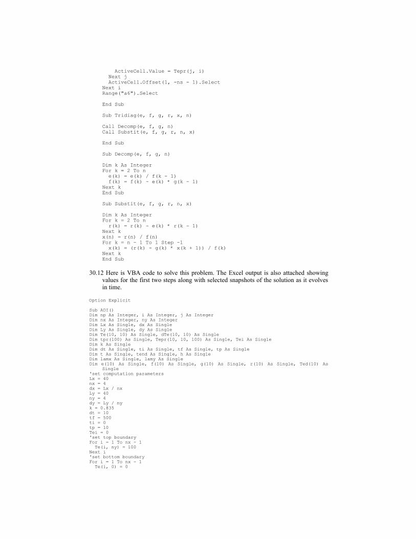
ActiveCell.Value = Tepr(j, i) Next j ActiveCell.Offset(1, -ns - 1).SelectNext iRange("a6").Select
End Sub
Sub Tridiag(e, f, g, r, x, n)
Call Decomp(e, f, g, n)Call Substit(e, f, g, r, n, x)
End Sub
Sub Decomp(e, f, g, n)
Dim k As IntegerFor k = 2 To n e(k) = e(k) / f(k - 1) f(k) = f(k) - e(k) * g(k - 1)Next kEnd Sub
Sub Substit(e, f, g, r, n, x)
Dim k As IntegerFor k = 2 To n r(k) = r(k) - e(k) * r(k - 1)Next kx(n) = r(n) / f(n)For k = n - 1 To 1 Step -1 x(k) = (r(k) - g(k) * x(k + 1)) / f(k)Next kEnd Sub
30.12 Here is VBA code to solve this problem. The Excel output is also attached showingvalues for the first two steps along with selected snapshots of the solution as it evolvesin time.
Option Explicit
Sub ADI()Dim np As Integer, i As Integer, j As IntegerDim nx As Integer, ny As IntegerDim Lx As Single, dx As SingleDim Ly As Single, dy As SingleDim Te(10, 10) As Single, dTe(10, 10) As SingleDim tpr(100) As Single, Tepr(10, 10, 100) As Single, Tei As SingleDim k As SingleDim dt As Single, ti As Single, tf As Single, tp As SingleDim t As Single, tend As Single, h As SingleDim lamx As Single, lamy As SingleDim e(10) As Single, f(10) As Single, g(10) As Single, r(10) As Single, Ted(10) As
Single'set computation parametersLx = 40nx = 4dx = Lx / nxLy = 40ny = 4dy = Ly / nyk = 0.835dt = 10tf = 500ti = 0tp = 10Tei = 0'set top boundaryFor i = 1 To nx - 1 Te(i, ny) = 100Next i'set bottom boundaryFor i = 1 To nx - 1 Te(i, 0) = 0

Next i'set left boundaryFor j = 1 To ny - 1 Te(0, j) = 75Next j'set right boundaryFor j = 1 To ny - 1 Te(nx, j) = 50Next j'set corners for plotTe(0, 0) = (dy * Te(1, 0) + dx * Te(0, 1)) / (dy + dx)Te(nx, 0) = (dy * Te(nx - 1, 0) + dx * Te(nx, 1)) / (dy + dx)Te(0, ny) = (dy * Te(1, ny) + dx * Te(0, ny - 1)) / (dy + dx)Te(nx, ny) = (dy * Te(nx - 1, ny) + dx * Te(nx, ny - 1)) / (dy + dx)'set interiorFor i = 1 To nx - 1 For j = 1 To ny - 1 Te(i, j) = Tei Next jNext i'save initial values for outputnp = 0t = titpr(np) = tFor i = 0 To nx For j = 0 To ny Tepr(i, j, np) = Te(i, j) Next jNext iDo tend = t + tp If tend > tf Then tend = tf h = dt Do If t + h > tend Then h = tend - t 'Sweep y lamx = k * h / dx ^ 2 lamy = k * h / dy ^ 2 For i = 1 To nx - 1 f(1) = 2 * (1 + lamy) g(1) = -lamy r(1) = lamx * Te(i - 1, 1) + 2 * (1 - lamx) * Te(i, 1) + lamx * Te(i + 1, 1) _ + lamy * Te(i, 0) For j = 2 To ny - 2 e(j) = -lamy f(j) = 2 * (1 + lamy) g(j) = -lamy r(j) = lamx * Te(i - 1, j) + 2 * (1 - lamx) * Te(i, j) + lamx * Te(i + 1, j) Next j e(ny - 1) = -lamy f(ny - 1) = 2 * (1 + lamy) r(ny - 1) = lamx * Te(i - 1, ny - 1) + 2 * (1 - lamx) * Te(i, ny - 1) _ + lamx * Te(i + 1, ny - 1) + lamy * Te(i, nx) Call Tridiag(e(), f(), g(), r(), Ted(), nx - 1) For j = 1 To ny - 1 Te(i, j) = Ted(j) Next j Next i t = t + h / 2 'Sweep x For j = 1 To ny - 1 f(1) = 2 * (1 + lamx) g(1) = -lamx r(1) = lamy * Te(1, j - 1) + 2 * (1 - lamy) * Te(1, j) + lamy * Te(1, j + 1) _ + lamx * Te(0, j) For i = 2 To nx - 2 e(i) = -lamx f(i) = 2 * (1 + lamx) g(i) = -lamx r(i) = lamy * Te(i, j - 1) + 2 * (1 - lamy) * Te(i, j) + lamy * Te(i, j + 1) Next i e(nx - 1) = -lamx f(nx - 1) = 2 * (1 + lamx) r(nx - 1) = lamy * Te(nx - 1, j - 1) + 2 * (1 - lamy) * Te(nx - 1, j) _ + lamy * Te(nx - 1, j + 1) + lamx * Te(ny, j) Call Tridiag(e(), f(), g(), r(), Ted(), nx - 1) For i = 1 To nx - 1 Te(i, j) = Ted(i) Next i Next j t = t + h / 2 If t >= tend Then Exit Do

Loop 'save values for output np = np + 1 tpr(np) = t For i = 0 To nx For j = 0 To ny Tepr(i, j, np) = Te(i, j) Next j Next i If t >= tf Then Exit DoLoop'output results back to sheetRange("a5").SelectRange("a5:e2005").ClearContentsFor k = 0 To np ActiveCell.Value = "t = " & tpr(k) ActiveCell.Offset(1, 0).Select For j = ny To 0 Step -1 For i = 0 To nx ActiveCell.Value = Tepr(i, j, k) ActiveCell.Offset(0, 1).Select Next i ActiveCell.Offset(1, -nx - 1).Select Next j ActiveCell.Offset(1, 0).SelectNext kRange("a5").SelectEnd Sub
Sub Tridiag(e, f, g, r, x, n)Call Decomp(e, f, g, n)Call Substit(e, f, g, r, n, x)End Sub
Sub Decomp(e, f, g, n)Dim k As IntegerFor k = 2 To n e(k) = e(k) / f(k - 1) f(k) = f(k) - e(k) * g(k - 1)Next kEnd Sub
Sub Substit(e, f, g, r, n, x)Dim k As IntegerFor k = 2 To n r(k) = r(k) - e(k) * r(k - 1)Next kx(n) = r(n) / f(n)For k = n - 1 To 1 Step -1 x(k) = (r(k) - g(k) * x(k + 1)) / f(k)Next kEnd Sub
30.13 MATLAB solution:
%PDE Parabolic Problem - Heat conduction in a rod% u[xx]=u[t]% BC u(0,t)=0 u(1,t)=1% IC u(x,0)=0 x<1
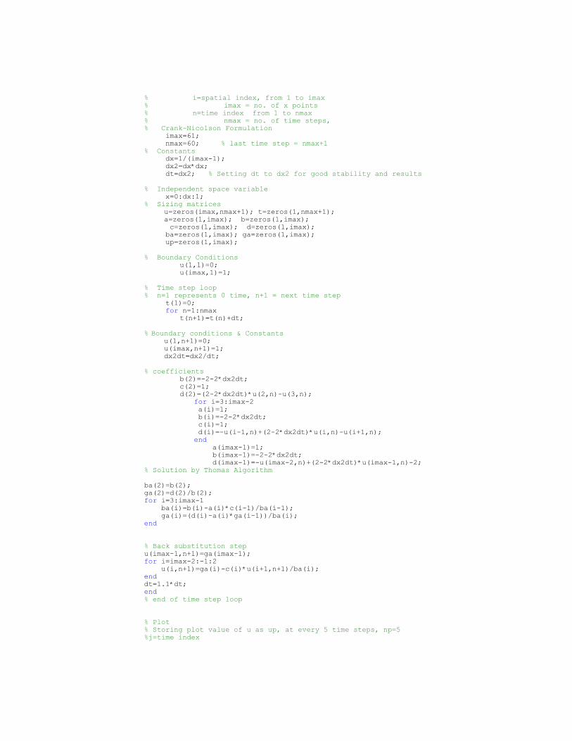
% i=spatial index, from 1 to imax % imax = no. of x points% n=time index from 1 to nmax% nmax = no. of time steps,% Crank-Nicolson Formulation
imax=61;nmax=60; % last time step = nmax+1
% Constantsdx=1/(imax-1); dx2=dx*dx;dt=dx2; % Setting dt to dx2 for good stability and results
% Independent space variablex=0:dx:1;
% Sizing matrices u=zeros(imax,nmax+1); t=zeros(1,nmax+1); a=zeros(1,imax); b=zeros(1,imax);
c=zeros(1,imax); d=zeros(1,imax);ba=zeros(1,imax); ga=zeros(1,imax);up=zeros(1,imax);
% Boundary Conditions u(1,1)=0; u(imax,1)=1;
% Time step loop% n=1 represents 0 time, n+1 = next time step
t(1)=0;for n=1:nmax
t(n+1)=t(n)+dt;
% Boundary conditions & Constants u(1,n+1)=0; u(imax,n+1)=1; dx2dt=dx2/dt;
% coefficients b(2)=-2-2*dx2dt; c(2)=1; d(2)=(2-2*dx2dt)*u(2,n)-u(3,n); for i=3:imax-2 a(i)=1; b(i)=-2-2*dx2dt; c(i)=1; d(i)=-u(i-1,n)+(2-2*dx2dt)*u(i,n)-u(i+1,n); end a(imax-1)=1; b(imax-1)=-2-2*dx2dt; d(imax-1)=-u(imax-2,n)+(2-2*dx2dt)*u(imax-1,n)-2;% Solution by Thomas Algorithm ba(2)=b(2);ga(2)=d(2)/b(2);for i=3:imax-1 ba(i)=b(i)-a(i)*c(i-1)/ba(i-1); ga(i)=(d(i)-a(i)*ga(i-1))/ba(i);end
% Back substitution stepu(imax-1,n+1)=ga(imax-1);for i=imax-2:-1:2 u(i,n+1)=ga(i)-c(i)*u(i+1,n+1)/ba(i);end dt=1.1*dt;end % end of time step loop
% Plot% Storing plot value of u as up, at every 5 time steps, np=5%j=time index
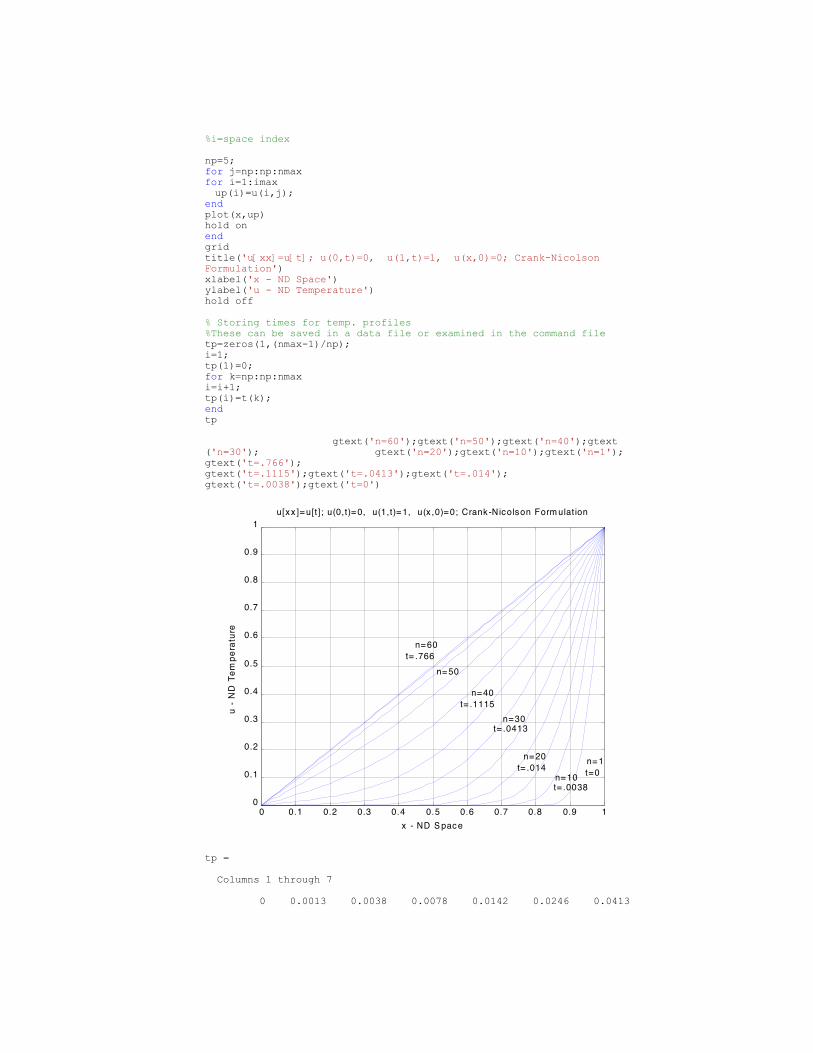
%i=space index
np=5;for j=np:np:nmaxfor i=1:imaxup(i)=u(i,j);
endplot(x,up)hold onendgridtitle('u[xx]=u[t]; u(0,t)=0, u(1,t)=1, u(x,0)=0; Crank-NicolsonFormulation')xlabel('x - ND Space')ylabel('u - ND Temperature')hold off
% Storing times for temp. profiles%These can be saved in a data file or examined in the command filetp=zeros(1,(nmax-1)/np);i=1;tp(1)=0;for k=np:np:nmaxi=i+1;tp(i)=t(k);endtp gtext('n=60');gtext('n=50');gtext('n=40');gtext('n=30'); gtext('n=20');gtext('n=10');gtext('n=1');gtext('t=.766');gtext('t=.1115');gtext('t=.0413');gtext('t=.014');gtext('t=.0038');gtext('t=0')
0 0.1 0.2 0.3 0.4 0.5 0.6 0.7 0.8 0.9 10
0.1
0.2
0.3
0.4
0.5
0.6
0.7
0.8
0.9
1u[xx ]= u[t ]; u(0,t)= 0, u(1,t)= 1, u(x ,0)=0; Crank -Nicolson Form ulat ion
x - ND S pac e
u - N
D T
empe
ratu
re
n=60
n= 50
n=40
n=30
n=20
n=10
n= 1
t= .766
t= .1115
t= .0413
t= .014
t= .0038t=0
tp =
Columns 1 through 7
0 0.0013 0.0038 0.0078 0.0142 0.0246 0.0413

Columns 8 through 13
0.0682 0.1115 0.1813 0.2937 0.4746 0.7661
30.14
t
u
r
u
rr
u
∂
∂=
∂
∂+
∂
∂ 12
2
Substituting of second order correct Crank-Nicolson analogues
t
uu
t
u
rir
r
uu
r
uu
r
u
r
uuu
r
uuu
r
u
nini
nininini
nininininini
∆
−=
∂
∂
∆−=
∆
−+
∆
−=
∂
∂
∆
+−+
∆
+−=
∂
∂
+
−++−++
−++−+++
,1,
,1,11,11,1
2
,1,,1
2
1,11,1,1
2
2
)1(
222
1
2
1
into the governing equation give the following finite difference equations:
nini
nininini
ui
ut
r
ui
ui
ut
ru
i
,1,
2
,11,11,
2
1,1
)1(2
1122
)1(2
11
)1(2
1122
)1(2
11
+
−++++−
−+−+
∆
∆−−
−+−=
−++
∆
∆−−+
−−
For the end points:
x = 1 (i = R), substitute the value of uR = 1 into the above FD equationx = 0 (i = 1), set the FD analog to the first derivative = 0
0222
1 ,0,21,01,2
1
=
∆
−+
∆
−=
∂
∂ ++
= r
uu
r
uu
r
u nnnn
i
Also substitute in i = 1 into the finite difference equation and algebraically eliminate
nn uu ,01,0 ++ from the two equations and get the FD equation at i = 1:
[ ] [ ] nnnn uut
ruu
t
r,2,1
2
1,21,1
2
222222 −+
∆
∆−−=+
∆
∆−− ++
%PDE Parabolic Problem - Heat conduction in the radial direction in acircular rod% u[rr]+(1/r)u[r]=u[t] 0<r<1% BC u(1,t)=1 u[r](0,t)=0% IC u(r,0)=0 0<r<1% i=spatial index, from 1 to imax % imax = no. of r points (imax=21 for 20 dr spaces)% n=time index from 1 to nmax% nmax = no. of time steps,% Crank-Nicolson Formulation
imax=41;nmax=60; % last time step = nmax+1

% Constants
dr=1/(imax-1); dr2=dr*dr;dt=dr2; % Setting dt to dr2 for good stability and results
% Independent space variabler=0:dr:1;
% Sizing matrices
u=zeros(imax,nmax+1); t=zeros(1,nmax+1);a=zeros(1,imax); b=zeros(1,imax);
c=zeros(1,imax); d=zeros(1,imax);ba=zeros(1,imax); ga=zeros(1,imax);up=zeros(1,imax);
% Boundary Conditions u(imax,1)=1;
% Time step loop% n=1 represents 0 time, new time = n+1
t(1)=0;for n=1:nmax t(n+1)=t(n)+dt;
% Boundary conditions & Constantsu(imax,n+1)=1;dr2dt=dr2/dt;
% coefficients b(1)=-2-2*dr2dt; c(1)=2; d(1)=(2-2*dr2dt)*u(1,n)-2*u(2,n); for i=2:imax-2 a(i)=1-1/(2*(i-1)); b(i)=-2-2*dr2dt; c(i)=1+1/(2*(i-1)); d(i)=(-1+1/(2*(i-1)))*u(i-1,n)+(2-2*dr2dt)*u(i,n)+(-1-1/(2*(i-1)))*u(i+1,n); end a(imax-1)=1-1/(2*(imax-2)); b(imax-1)=-2-2*dr2dt; d(imax-1)=(-1+1/(2*(imax-2)))*u(imax-2,n)+(2-2*dr2dt)*u(imax-1,n)-2*(1+1/(2*(imax-2)))% Solution by Thomas Algorithm ba(1)=b(1); ga(1)=d(1)/b(1); for i=2:imax-1 ba(i)=b(i)-a(i)*c(i-1)/ba(i-1); ga(i)=(d(i)-a(i)*ga(i-1))/ba(i); end
% Back substitution step u(imax-1,n+1)=ga(imax-1); for i=imax-2:-1:1 u(i,n+1)=ga(i)-c(i)*u(i+1,n+1)/ba(i); end dt=1.1*dt;
end % end of time step loop
% Plot% Storing plot value of u as up, at every 5 time steps%j=time index%i=space index
istart=4;for j=istart:istart:nmax+1
for i=1:imax up(i)=u(i,j);
endplot(r,up)

hold onendgrid
title('u[rr]+(1/r)u[r]=u[t]; u(1,t)=1 u[r](0,t)=0; u(r,0)=0')xlabel('r - ND Space')ylabel('u - ND Temperature')hold off
% Storing times for temp. profiles% These can be saved in a data file or examined in the command file
tp=zeros(1,(nmax-1)/istart);i=1;tp(1)=0;for k=istart:istart:nmax+1
i=i+1;tp(i)=t(k);
endtp
0 0.1 0.2 0.3 0.4 0.5 0.6 0.7 0.8 0.9 10
0.1
0.2
0.3
0.4
0.5
0.6
0.7
0.8
0.9
1u[rr]+ (1/r)u[r]= u[t ]; u(1,t)= 1 u[r](0,t)= 0; u(r,0)=0
r - ND S pac e
u -
ND
Tem
pera
ture
tp =
Columns 1 through 7
0 0.0021 0.0059 0.0116 0.0199 0.0320 0.0497
Columns 8 through 14
0.0757 0.1137 0.1694 0.2509 0.3703 0.5450 0.8008
Columns 15 through 16
1.1754 1.7238
30.15

t
u
x
ub
dx
u
∂
∂=
∂
∂+
∂2
2
Substituting of second order correct Crank-Nicolson analogues
t
uu
t
u
x
uu
x
uu
x
u
x
uuu
x
uuu
x
u
nini
nininini
nininininini
∆
−=
∂
∂
∆
−+
∆
−=
∂
∂
∆
+−+
∆
+−=
∂
∂
+
−++−++
−++−+++
,1,
,1,11,11,1
2
,1,,1
2
1,11,1,1
2
2
222
1
2
1
into the governing equation give the following finite difference equations
nini
nininini
uxbut
x
uxbuxbut
xuxb
,1,
2
,11,11,
2
1,1
2
1122
2
11
2
1122
2
11
+
−++++−
∆−−+
∆
∆−+
∆+−=
∆++
∆
∆−−+
∆−
%PDE Parabolic Problem with a dispersion term% u[xx]+bu[x]=u[t]% BC u(0,t)=0 u(1,t)=1% IC u(x,0)=0 x<1% i=spatial index, from 1 to imax % imax = no. of spatial points (imax=21 for 20 dx spaces)% n=time index, from 1 to nmax% nmax = no. of time steps% Crank-Nicholson formulation for the spatial derivatives
imax=61;nmax=60; % last time step = nmax+1
% constants
dx=1/(imax-1);dx2=dx*dx;dt=dx2;
% ParametersB=-4;
% Independent spatial variablex=0:dx:1;
% Sizing matricesu=zeros(imax,nmax); t=zeros(1,nmax);a=zeros(1,imax); b=zeros(1,imax);
c=zeros(1,imax); d=zeros(1,imax);ba=zeros(1,imax); ga=zeros(1,imax);up=zeros(1,imax);
% Boundary Conditions u(1,1)=0; u(imax,1)=1;
% Time step loop% n=1 represents 0 time, new time = n+1
t(1)=0; for n=1:nmax

t(n+1)=t(n)+dt;
% Boundary conditions & constantsu(1,n+1)=0;u(imax,n+1)=1;dx2dt=dx2/dt;
% Coefficients b(2)=-2-2*dx2dt; c(2)=1+0.5*B*dx; d(2)=(-1-0.5*B*dx)*u(3,n)+(2-2*dx2dt)*u(2,n); for i=3:imax-2 a(i)=1-0.5*B*dx; b(i)=-2-2*dx2dt; c(i)=1+0.5*B*dx; d(i)=(-1-0.5*B*dx)*u(i+1,n)+(2-2*dx2dt)*u(i,n)+(-1+0.5*B*dx)*u(i-1,n); end a(imax-1)=1-0.5*B*dx;b(imax-1)=-2-2*dx2dt;d(imax-1)=2*(-1-0.5*B*dx)+(2-2*dx2dt)*u(imax-1,n)+(-1+0.5*B*dx)*u(imax-2,n);
% Solution by Thomas Algorithm ba(2)=b(2); ga(2)=d(2)/b(2); for i=3:imax-1 ba(i)=b(i)-a(i)*c(i-1)/ba(i-1); ga(i)=(d(i)-a(i)*ga(i-1))/ba(i); end
% Back substitution step u(imax-1,n+1)=ga(imax-1); for i=imax-2:-1:2 u(i,n+1)=ga(i)-c(i)*u(i+1,n+1)/ba(i); end dt=1.1*dt;
end% End of time step loop
%Plot%Storing plot value of u as up, at ever 5 time steps% j=time index% i=speace index
for j=5:5:nmaxfor i=1:imax
up(i)=u(i,j);end
plot(x,up)hold on
endgrid
title('u[xx]+bu[x]=u[t]; u(0,t)=0 u(1,t)=1; u(x,0)=0 x<1')xlabel('x - ND Space')ylabel('u - ND Temperature')hold offgtext('b=-4')% Storing times for temp. profiles% These can be used in a data file or examined in the command file
tp=zeros(1,(nmax-1)/5);i=1;tp(1)=0;for k=5:5:nmax
i=i+1;tp(i)=t(k);
endtp
tp =

Columns 1 through 7
0 0.0013 0.0038 0.0078 0.0142 0.0246 0.0413
Columns 8 through 13
0.0682 0.1115 0.1813 0.2937 0.4746 0.7661
0 0.1 0.2 0.3 0.4 0.5 0.6 0.7 0.8 0.9 10
0.1
0.2
0.3
0.4
0.5
0.6
0.7
0.8
0.9
1u[x x ]+bu[x ]= u[t] ; u(0,t)= 0 u(1,t)= 1; u(x ,0)= 0 x<1
x - ND S pace
u -
ND
Tem
pera
ture
b=4
0 0.1 0.2 0.3 0.4 0.5 0.6 0.7 0.8 0.9 10
0.1
0.2
0.3
0.4
0.5
0.6
0.7
0.8
0.9
1u[x x ]+ bu[x ]= u[t]; u(0,t)= 0 u(1,t)= 1; u(x ,0)= 0 x < 1
x - ND S pac e
u -
ND
Tem
pera
ture
b= 2

0 0.1 0.2 0.3 0.4 0.5 0.6 0.7 0.8 0.9 10
0.1
0.2
0.3
0.4
0.5
0.6
0.7
0.8
0.9
1u[x x ]+bu[x ]= u[t]; u(0,t)=0 u(1,t)= 1; u(x ,0)= 0 x< 1
x - ND S pac e
u - N
D T
empe
ratu
re
b=0
0 0.1 0.2 0.3 0.4 0.5 0.6 0.7 0.8 0.9 10
0.1
0.2
0.3
0.4
0.5
0.6
0.7
0.8
0.9
1u[x x ]+bu[x ]= u[t]; u(0,t)=0 u(1,t)= 1; u(x ,0)= 0 x< 1
x - ND S pac e
u - N
D T
empe
ratu
re
b= -2

0 0.1 0.2 0.3 0.4 0.5 0.6 0.7 0.8 0.9 10
0.1
0.2
0.3
0.4
0.5
0.6
0.7
0.8
0.9
1u[x x ]+bu[x ]= u[t]; u(0,t)=0 u(1,t)= 1; u(x ,0)= 0 x< 1
x - ND S pac e
u - N
D T
empe
ratu
re
b= -4

CHAPTER 31
31.1 The equation to be solved is
d T
dx
2
220= −
Assume a solution of the form T = ax2 + bx + c which can be differentiated twice to give T” = 2a.
Substituting this result into the differential equation gives a = −10. The boundary conditions canbe used to evaluate the remaining coefficients. For the first condition at x = 0,
50 10 0 02= − + +( ) ( )b c
or c = 50. Similarly, for the second condition.
100 10 10 10 502= − + +( ) ( )b
which can be solved for b = 105. Therefore, the final solution is
T x x= − + +10 105 502
The results are plotted in Fig. 31.5.
0
100
200
300
0 5 10
31.2 The heat source term in the first row of Eq. (31.26) can be evaluated by substituting Eq. (31.3)and integrating to give
202 5
2 525
0
2 5 .
.
. −=∫
xdx
Similarly, Eq. (31.4) can be substituted into the heat source term of the second row of Eq.(31.26), which can also be integrated to yield
200
2 525
0
2 5 xdx
−=∫ .
.
These results along with the other parameter values can be substituted into Eq. (31.26) to give
0 4 0 4 251 2 1
. . ( )T TdT
dxx− = − +
and

− + = +0 4 0 4 251 2 2
. . ( )T TdT
dxx
31.3 In a manner similar to Fig. 31.7, the equations can be assembled for the total system,
0 4 0 4
0 4 0 8 0 4
0 4 0 8 0 4
0 4 08 0 4
0 4 0 4
25
50
50
50
25
1
2
3
4
5
1
1
. .
. . .
. . .
. . .
. .
( ) /
( ) /
−
− −
− −
− −
−
=
− +
+
T
T
T
T
T
dT x dx
dT x dx
The unknown end temperatures can be substituted to give
1 0 4
0 8 0 4
0 4 0 8 0 4
0 4 0 8
0 4 1
5
70
50
90
15
1
2
3
4
5
−
−
− −
−
− −
−
=
−
.
. .
. . .
. .
.
( ) /
( ) /
dT x dx
T
T
T
dT x dx
These equations can be solved for
dT x dx
T
T
T
dT x dx
( ) /
( ) /
1
2
3
4
5
105
250
325
275
95−
=
−
The solution, along with the analytical solution (dashed line) is shown below:
0
100
200
300
0 5 10
31.4
02
2= − −D
d c
dxUdc
dxkc
R Dd c
dxUdc
dxkc= − −
2
2
~ ~~
Dd c
dxUdc
dxkc N dx
x
x
i
2
21
2~ ~
~− −
∫

Dd c
dxN x dxi
x
x 2
21
2~
( )∫ (1)
− ∫Udc
dxN x dxi
x
x ~( )
1
2
(2)
− ∫k cN x dxix
x~ ( )
1
2
(3)
Term (1):
Dd c
dxN x dx D
dc
dxx
c c
x x
dc
dxx
c c
x x
ix
x 2
2
11 2
2 1
22 1
2 1
1
2~
( )
( )
( )∫ =
− −−
−
−−
−
Term (2):
dc
dxN x dx
c c
x xN x dxi
x
x
ix
x~( ) ( )
1
2
1
2 2 1
2 1∫ ∫=
−
−
N x dxx x
ix
x
( )1
2 2 1
2∫ =−
∴ =−
∫dc
dxN x dx
c ci
x
x ~( )
1
2 2 1
2
− = −
−
−
∫Udc
dxN x dx U
c c
c cix
x ~( )
1
2
2 1
2 1
2
2
Term (3):
− = −−
∫k c N x dxk x x c
ci
x
x~ ( )
( )2 1 1
221
2
Total element equation [(1) + (2) + (3)]
a a
a a
c
c
b
b
11 11
11 11
1
2
1
2
=
where
( )aD
x x
U kx x11
2 1
2 12 2
=−
− + − aD
x x
U12
2 1 2=
−
−+ a
D
x x
U21
2 1 2=
−
−−
( )aD
x x
U kx x22
2 1
2 12 2
= −−
+ + −

b Ddc
dxx1 1= − ( ) b D
dc
dxx2 2= ( )
31.5 First we can develop an analytical function for comparison. Substituting parameters gives
15 10 5082
2. × =
d u
dx
Assume a solution of the form
u ax bx c= + +2
This can be differentiated twice to yield d2u/dx2 = 2a. This can be substituted into the ODE,
which can then be solved for a = 1.6667×10⁻⁷. The boundary conditions can then be used to
evaluate the remaining coefficients. At the left side, u(0) = 0 and
0 16667 10 0 07 2= × + +−. ( ) ( )b c
and therefore, c = 0. At the right side of the bar, u(30) = 0 and
0 16667 10 30 307 2= × +−. ( ) ( )b
and therefore, b = −5×10⁻⁶, and the solution is
u x x= × − ×− −16667 10 5 107 2 6.
which can be displayed as
-4E-05
-2E-05
0E+00
0 6 12 18 24 30
The element equation can be written as
A E
x x
u
uA E
du
dxx
du
dxx
P x N x dx
P x N x dx
cc
x
x
x
x2 1
1
2
1
2
1
2
1 1
1 11
2
1
2−
−
−
=
−
+
∫∫
( )
( )
( ) ( )
( ) ( )
The distributed load can be evaluated as
−−
= − −−
= −∫ ∫506
6150 50
0
6150
0
6
0
6xdx
xdx
Thus, the final element equation is

2 5 10 2 5 10
2 5 10 2 5 10
150
150
7 7
7 7
1
2
1
2
. .
. .
( )
( )
× − ×
− × ×
=
−
+
−
−
u
uA E
du
dxx
du
dxx
c
Assembly yields
15 10 2 5 10
5 10 2 5 10
2 5 10 5 10 2 5 10
2 5 10 5 10 2 5 10
2 5 10 5 10
2 5 10 15 10
150
300
300
300
300
150
8 7
7 7
7 7 7
7 7 7
7 7
7 7
1
1
1
1
1
2
. .
.
. .
. .
.
. .
( )
( )
× − ×
× − ×
− × × − ×
− × × − ×
− × ×
− × − ×
=
−
−
−
−
−
−
du
dxx
u
u
u
u
du
dxx
which can be solved for
du
dxx
u
u
u
u
du
dxx
( )
( )
.
.
.
.
1
1
1
1
1
2
6
5
5
5
5
6
5 10
2 4 10
36 10
36 10
2 4 10
5 10
=
− ×
− ×
− ×
− ×
− ×
×
−
−
−
−
−
−
These results, along with the analytical solution (dashed line) are displayed below:
-4E-05
-2E-05
0E+00
0 6 12 18 24 30
31.6 Option Explicit
Sub FErod()
Dim ns As Integer, ii As Integer, i As Integer, j As IntegerDim k As Integer, m As IntegerDim x(5) As Single, st(2, 2) As Single, c As SingleDim s(2, 2) As Single, a(5, 5) As Single, b(5) As Single, d(5) As SingleDim Te(5) As Single, ff As SingleDim e(5) As Single, f(5) As Single, g(5) As Single, r(5) As SingleDim dum1 As Single, dum2 As SingleDim dTeLeft As Single, dTeRight As Single
'set parameters

ns = 4x(1) = 0x(2) = 2.5x(3) = 5x(4) = 7.5x(5) = 10Te(1) = 40Te(5) = 200ff = 10
'construct system matrixst(1, 1) = 1: st(1, 2) = -1: st(2, 1) = -1: st(2, 2) = 1For ii = 1 To ns c = 1 / (x(ii + 1) - x(ii)) For i = 1 To 2 For j = 1 To 2 s(i, j) = c * st(i, j) Next j Next i For i = 1 To 2 k = ii - 1 + i For j = 1 To 2 m = ii - 1 + j a(k, m) = a(k, m) + s(i, j) Next j b(k) = b(k) + ff * ((x(ii + 1) - x(ii)) - (x(ii + 1) - x(ii)) / 2) Next iNext ii
'determine impact of uniform source and boundary conditionsCall Mmult(a(), Te(), d(), ns + 1, ns + 1, 1)For i = 1 To ns + 1 b(i) = b(i) - d(i)Next ia(1, 1) = 1a(2, 1) = 0a(ns + 1, ns + 1) = -1a(ns, ns + 1) = 0
'Transform square matrix into tridiagonal formf(1) = a(1, 1)g(1) = a(1, 2)r(1) = b(1)For i = 2 To ns e(i) = a(i, i - 1) f(i) = a(i, i) g(i) = a(i, i + 1) r(i) = b(i)Next ie(ns + 1) = a(ns + 1, ns)f(ns + 1) = a(ns + 1, ns + 1)r(ns + 1) = b(ns + 1)
'Tridiagonal solverdum1 = Te(1)dum2 = Te(ns + 1)Call Tridiag(e, f, g, r, ns + 1, Te())dTeLeft = Te(1)dTeRight = Te(ns + 1)Te(1) = dum1Te(ns + 1) = dum2
'output resultsRange("a3").SelectActiveCell.Value = "dTe(x = " & x(0) & ")/dx = "ActiveCell.Offset(0, 1).SelectActiveCell.Value = dTeLeftActiveCell.Offset(1, -1).SelectActiveCell.Value = "dTe(x = " & x(ns + 1) & ")/dx = "ActiveCell.Offset(0, 1).SelectActiveCell.Value = dTeRightActiveCell.Offset(3, -1).Select

For i = 1 To ns + 1 ActiveCell.Value = x(i) ActiveCell.Offset(0, 1).Select ActiveCell.Value = Te(i) ActiveCell.Offset(1, -1).SelectNext iRange("b3").Select
End Sub
Sub Mmult(a, b, c, m, n, l)
Dim i As Integer, j As Integer, k As IntegerDim sum As Single
For i = 1 To n sum = 0 For k = 1 To m sum = sum + a(i, k) * b(k) Next k c(i) = sumNext i
End Sub
Sub Tridiag(e, f, g, r, n, x)Dim k As Integer
'decomposeFor k = 2 To n e(k) = e(k) / f(k - 1) f(k) = f(k) - e(k) * g(k - 1)Next k'substituteFor k = 2 To n r(k) = r(k) - e(k) * r(k - 1)Next kx(n) = r(n) / f(n)For k = n - 1 To 1 Step -1 x(k) = (r(k) - g(k) * x(k + 1)) / f(k)Next kEnd Sub
The output is
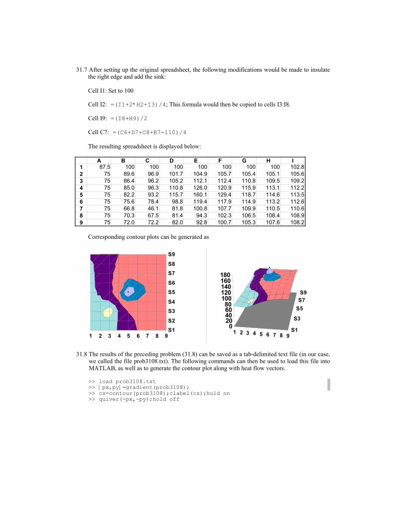
31.7 After setting up the original spreadsheet, the following modifications would be made to insulatethe right edge and add the sink:
Cell I1: Set to 100
Cell I2: =(I1+2*H2+I3)/4; This formula would then be copied to cells I3:I8.
Cell I9: =(I8+H9)/2
Cell C7: =(C6+D7+C8+B7-110)/4
The resulting spreadsheet is displayed below:
A B C D E F G H I
1 87.5 100 100 100 100 100 100 100 102.8
2 75 89.6 96.9 101.7 104.9 105.7 105.4 105.1 105.6
3 75 86.4 96.2 105.2 112.1 112.4 110.8 109.5 109.2
4 75 85.0 96.3 110.8 126.0 120.9 115.9 113.1 112.2
5 75 82.2 93.2 115.7 160.1 129.4 118.7 114.6 113.5
6 75 75.6 78.4 98.8 119.4 117.9 114.9 113.2 112.6
7 75 66.8 46.1 81.8 100.8 107.7 109.9 110.5 110.6
8 75 70.3 67.5 81.4 94.3 102.3 106.5 108.4 108.9
9 75 72.0 72.2 82.0 92.8 100.7 105.3 107.6 108.2
Corresponding contour plots can be generated as
1 2 3 4 5 6 7 8 9
S1
S2
S3
S4
S5
S6
S7
S8
S9
1 2 3 4 5 6 7 8 9
S1
S3
S5
S7
S9
020406080
100
120
140
160
180
31.8 The results of the preceding problem (31.8) can be saved as a tab-delimited text file (in our case,we called the file prob3108.txt). The following commands can then be used to load this file intoMATLAB, as well as to generate the contour plot along with heat flow vectors.
>> load prob3108.txt>> [px,py]=gradient(prob3108);>> cs=contour(prob3108);clabel(cs);hold on>> quiver(-px,-py);hold off

1 2 3 4 5 6 7 8 9
1
2
3
4
5
6
7
8
9
60
80
100
120 140
160
31.9 The scheme for implementing this calculation on Excel is shown below:
A B C D E F G H I J K
1 87.5 100 100 100 100 100 100 100 100 100 62.5
2 75 25
3 75 25
4 75 25
5 75 25
6 62.5 50 50 50 50 50 50 50 50 50 37.5
The simple Laplace equation applies directly to the blank white cells (recall Fig. 31.14).However, for the shaded cells impacted by the heat sink, a heat balance equation must bewritten. For example, for cell E3, the control volume approach can be developed as
03 3 3 3 3 4 2 3
100= −−
+−
−−
+−
−kE D
xy z k
F D
xy z k
E E
yx z k
E E
yx z x y' ' ' '
∆∆ ∆
∆∆ ∆
∆∆ ∆
∆∆ ∆ ∆ ∆
Collecting and canceling terms yields
0 4 3 3 3 4 3 100= − + + + + −E D F E Dx y
zk
∆ ∆
∆ '
Substituting the length dimensions and the coefficient of thermal conductivity gives,
ED F E D
33 3 4 3 160
4=
+ + + −
The result is depicted below, along with the corresponding contour plots.
A B C D E F G H I J K
1 87.5 100 100 100 100 100 100 100 100 100 62.5
2 75 74.0 62.0 40.2 10.1 -1.5 7.9 34.7 50.8 51.3 25
3 75 59.0 33.7 -11.2 -98.2 -123.8 -101.8 -19.8 17.3 29.2 25
4 75 53.1 25.3 -20.7 -108.0 -133.7 -111.6 -29.2 8.8 23.4 25
5 75 53.3 34.9 11.2 -19.5 -31.3 -21.8 5.7 23.8 30.5 25
6 62.5 50 50 50 50 50 50 50 50 50 37.5
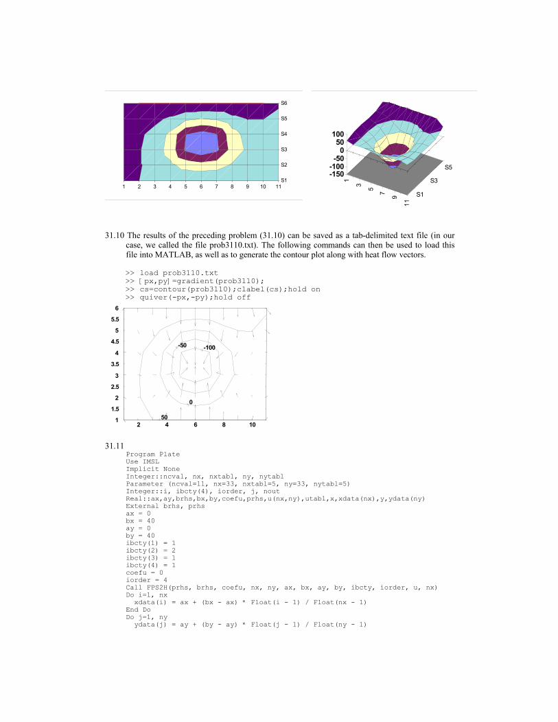
1 2 3 4 5 6 7 8 9 10 11
S1
S2
S3
S4
S5
S6
1
3
5
7
9
11
S1
S3
S5
-150
-100
-50
0
50
100
31.10 The results of the preceding problem (31.10) can be saved as a tab-delimited text file (in ourcase, we called the file prob3110.txt). The following commands can then be used to load thisfile into MATLAB, as well as to generate the contour plot along with heat flow vectors.
>> load prob3110.txt>> [px,py]=gradient(prob3110);>> cs=contour(prob3110);clabel(cs);hold on>> quiver(-px,-py);hold off
2 4 6 8 101
1.5
2
2.5
3
3.5
4
4.5
5
5.5
6
-100 -50
0
50
31.11Program PlateUse IMSLImplicit NoneInteger::ncval, nx, nxtabl, ny, nytablParameter (ncval=11, nx=33, nxtabl=5, ny=33, nytabl=5)Integer::i, ibcty(4), iorder, j, noutReal::ax,ay,brhs,bx,by,coefu,prhs,u(nx,ny),utabl,x,xdata(nx),y,ydata(ny)External brhs, prhsax = 0bx = 40ay = 0by = 40ibcty(1) = 1ibcty(2) = 2ibcty(3) = 1ibcty(4) = 1coefu = 0iorder = 4Call FPS2H(prhs, brhs, coefu, nx, ny, ax, bx, ay, by, ibcty, iorder, u, nx)Do i=1, nx xdata(i) = ax + (bx - ax) * Float(i - 1) / Float(nx - 1)End DoDo j=1, ny ydata(j) = ay + (by - ay) * Float(j - 1) / Float(ny - 1)

End DoCall UMACH(2, nout)Write (nout,'(8X,A,11X,A,11X,A)') 'X', 'Y', 'U'Do j=1, nytabl Do i=1, nxtabl x = ax + (bx - ax) * Float(i - 1) / Float(nxtabl - 1) y = ay + (by - ay) * Float(j - 1) / Float(nytabl - 1) utabl = QD2VL(x,y,nx,xdata,ny,ydata,u,nx,.FALSE.) Write (nout,'(4F12.4)') x, y, utabl End DoEnd DoEnd Program
Function prhs(x, y)Implicit NoneReal::prhs, x, yprhs = 0End Function
Real Function brhs(iside, x, y)Implicit NoneInteger::isideReal::x , yIf (iside == 1) Then brhs = 50ElseIf (iside == 2) Then brhs = 0ElseIf (iside == 3) Then brhs = 75Else brhs = 100End IfEnd Function
Output:
0.0000 0.0000 75.0000 10.0000 0.0000 71.6339 20.0000 0.0000 66.6152 30.0000 0.0000 59.1933 40.0000 0.0000 50.0000 0.0000 10.0000 75.0000 10.0000 10.0000 72.5423 20.0000 10.0000 67.9412 30.0000 10.0000 60.1914 40.0000 10.0000 50.0000 0.0000 20.0000 75.0000 10.0000 20.0000 75.8115 20.0000 20.0000 72.6947 30.0000 20.0000 64.0001 40.0000 20.0000 50.0000 0.0000 30.0000 75.0000 10.0000 30.0000 83.5385 20.0000 30.0000 83.0789 30.0000 30.0000 74.3008 40.0000 30.0000 50.0000 0.0000 40.0000 87.5000 10.0000 40.0000 100.0000 20.0000 40.0000 100.0000 30.0000 40.0000 100.0000 40.0000 40.0000 75.0000Press any key to continue

31.12
Other node equations are derived similarly


31.13
Other node equations are derived similarly