Embed Size (px)
Citation preview


Part III
Human Genetics

9
Mapping Qualitative Traits in Humans UsingAffected Sib Pairs
In humans we cannot create inbred lines, backcrosses, etc. Consequently, itis more difficult to study directly the correlation of phenotypes and geneticmarkers. We can proceed indirectly by noting that relatives frequently havemore similar phenotypes than non-relatives, presumably because they havemore similar genotypes. For studying human diseases, particularly convenientunits are affected sib pairs (ASP), which are the subject of this chapter. Wedelay until Chap. 11 a discussion of the substantially more complex problemof pedigrees involving variable numbers and relationships of affecteds.
Since humans are members of populations, not subject to breeding experi-ments, we shall want to use some of the material on population genetics fromChap. 3, notably that concerned with the ideas of random mating/Hardy-Weinberg equilibrium and identity by descent (IBD).
If two relatives are affected with the same disease, which is caused to someextent by the individual’s genotype and is relatively rare in the population,it seems plausible to hypothesize that they have the disease because bothinherited one or more disease-predisposing alleles from a common ancestor.
Recall that two relatives are said to have inherited an allele identical bydescent (IBD) at a given locus, if they have inherited the same allele froma common ancestor. At any genetic locus, two siblings inherit their paternalallele IBD with probability 1/2 and independently inherit their maternal al-lele IBD with probability 1/2. Thus they inherit 0, 1, or 2 alleles IBD withprobabilities 1/4, 1/2, 1/4, respectively; and on average they inherit one alleleIBD. (This argument presupposes that the parents are not inbred, so they donot already contain alleles inherited IBD from a remote ancestor.) If we havea sample of, say, n sib pairs, at a randomly selected genetic marker, there willbe about n alleles inherited IBD. If the sib pairs share a given phenotype,e.g., the same disease, then we expect that at a marker tightly linked to agene or genes contributing to the phenotype there will be more than n allelesIBD. In the following sections we develop a genetic model for a qualitativetrait and discuss genome scans to detect genes contributing to the trait. For
186 9 Mapping Qualitative Traits in Humans Using Affected Sib Pairs
simplicity we refer to the trait as a disease and individuals having the diseaseas affected. Analysis of QTL in humans is discussed in Chap. 11.
We use a simple genetic model in order to describe a potential connectionbetween the disease status of the siblings and the distribution of the num-ber of alleles shared IBD. This connection is then used in order to derive theconditional distribution of the number of alleles shared IBD, given that bothsiblings are affected. This leads in turn to a relation that connects the fre-quency in the population of the susceptibility alleles and their contribution tothe risk of getting the disease to the distribution of the test statistics. Theseissues are discussed in the following two sections.
The third section deals with the asymptotic distribution of the test statis-tic, and the properties of the associated test, when large samples are used inorder to detect a risk factor that has a relatively small effect on the probabilityof being affected.
The IBD status for a pair at a given locus is inferred from the genotypicinformation at hand, which may include the genotypes of the siblings andtheir parents or the genotypes of the siblings alone. In the preceding discussionwe make the assumption that the IBD status can be perfectly reconstructedbased on the genotypic information. In practice, this is seldom the case andan estimate of the IBD number has to replace the unknown true value. Inthe fourth section we will present statistical tools for the estimation of theIBD state from the genotypic information and assess the effect of partialinformation on the statistical properties of the scanning procedure.
9.1 Genetic Models
We assume initially a single susceptibility locus. The polymorphism at thatlocus consists of two alleles – a susceptibility allele D, and wild-type alleled. The genetic model provides the ingredients which are needed in order tocompute the conditional distribution of the IBD status, given the phenotypesof the siblings. It consists of two components: a model connecting phenotypesto genotypes at the susceptibility locus and a population genetic model, de-scribing the population joint distribution of genotypes at the trait loci for theparents of the siblings. Although we discuss in detail the case of a bi-allelicdisease locus, essentially all the results described are valid for loci having anarbitrary number of alleles.
A Model for the Trait
Here we consider a single autosomal trait locus with allele D, associated withthe disease, and a wild-type allele d. In the model we allow for sporadic casesand partial penetrance. Specifically, define the three penetrance probabilities:
9.1 Genetic Models 187
g0 = Pr(Affected | dd ) ,
g1 = Pr(Affected |Dd ) ,
g2 = Pr(Affected |DD) .
In order to emphasize certain similarities with the models used for experimen-tal genetics, it is often convenient to re-write the penetrances in the form
g1 = g0 + α + δ; g2 = g0 + 2α .
We assume that α > 0 to be consistent with g2 > g0. With this notation y,which refers here to the probability that an individual is affected as a functionof genotype, has the form of equation (2.2) with e = 0. Now xM (resp. xF)equals the number of D alleles, 0 or 1, inherited from the mother (resp. father).Note, however, that while in Chap. 2 y is an observed quantitative phenotypethat is allowed to take on any value, here the phenotype is 0 (no disease) or 1(disease), while y is the unobserved (conditional on the genotype) probabilitythat the phenotype is 1. Hence y itself must be between 0 and 1.
The additive model, which we emphasize in what follows, relates the threepenetrance parameters to each other by requiring that g1 = (g0 + g2)/2, orequivalently that δ = 0. Thus, one needs to specify only g0 and α. Moreover,as we shall see later, the quantity of interest will depend only on the ratioR2 = g2/g0 = 1 + 2α/g0 – the relative risk of a risk-allele homozygote withrespect to a wild-type homozygote. One can envision other special cases ofthis model, even in the simple case of a single trait locus. Important examplesare the recessive model which assumes g0 = g1 < g2, equivalently δ = −α orthe dominant model, which assumes g0 < g1 = g2, or δ = α. The statisticwe consider below, which counts the total number of alleles shared IBD, ismost appropriate for the additive model and to a good approximation for adominant model as well.
We complete the description of the relation between the genotypes andthe probability that the siblings are affected by adding the assumption thatwithin a pedigree, the phenotypes of relatives are conditionally independentgiven their genotypes. As a result, we find that
Pr(Both affected |G1, G2) = Pr(Affected |G1)× Pr(Affected |G2) = y1y2 ,(9.1)
where G1 and G2 are the genotypes of the first and the second sibling re-spectively. An important consequence of this assumption is the exclusion ofenvironmental effects on susceptibility to the disease. (See Prob. 9.5 for pos-sible generalizations.)
A Population Genetic Model
The second component in the genetic model is a population genetic model thatdescribes the frequencies of the pedigree founders’ genotypes. For the case of
188 9 Mapping Qualitative Traits in Humans Using Affected Sib Pairs
a sib-pair, there are two founders – the mother and the father, whom weassume mate at random in an infinitely large population and are themselvesthe product of random matings. Hence their genotypes are in Hardy-Weinbergequilibrium, i.e., the two alleles at a given locus are randomly sampled fromthe population pool. If the population frequency of the allele D is denotedby p (and the frequency of the allele d is 1 − p), then the probability ofthe genotype DD is p2. Likewise, the probability of the genotype dd is (1 −p)2, and the probability of the genotype Dd is 2 p(1 − p). Random matingalso implies independence between the parents’ genotypes. For example, theprobability that both parents’ genotypes are DD is p4. In a similar fashion, onecan compute the probability of all other combinations of parents’ genotypesas a function of a single parameter p, the frequency of the allele D in thegenetic pool. It also follows that each child individually has a genotype thatsatisfies Hardy-Weinberg frequencies. However, the genotypes of two childrenare dependent.
From (2.2), we obtain (2.3), which for convenience we repeat here (withe = 0):
y = m + {α + (1− 2p)δ}[(xM − p) + (xF − p)]− {2δ}[(xM − p)(xF − p)] .
Combining this expression with the assumption of Hardy-Weinberg equilib-rium, we also obtain the variance decomposition (2.5):
σ2y = σ2
A + σ2D ,
where σ2A = 2p(1− p)[α + (1− 2p)δ]2 and σ2
D = 4p2(1− p)2δ2. For a dominanttrait (δ = α) σ2
A = 8p(1 − p)3α2, while for a recessive trait (δ = −α) σ2A =
8p3(1 − p)α2. In the usual case that p is substantially less than 1/2, theadditive variance is much larger than the dominance variance for a dominanttrait, smaller for a recessive trait. The simplest case is an additive trait, forwhich δ = 0, hence σ2
D = 0.By taking expectations in (9.1) and using the representation of yi given
above to obtain an expression for the product y1y2, we can calculate theprobability Pr(A) that two sibs are both affected:
Pr(A) = E(y1y2) = m2 + cov(y1, y1) = m2 + σ2A/2 + σ2
D/4 . (9.2)
To see how (9.2) is derived, let xMi (xFi) denote the number of D allelesinherited by the ith sib from their mother (father). First recall that E[(xMi −p)2] = p(1−p). Now consider the product (xM1−p)(xM2−p). If xM1 and xM2 areIBD, then the product equals (xM1− p)2, so in this case the expected productis just p(1 − p), as before. If xM1 and xM2 are not IBD, then by the Hardy-Weinberg assumption, they are independent and the expected product is theproduct of the expectations, which equals 0. Since xM1 and xM2 are IBD withprobability 1/2, we find that E(xM1−p)(xM2−p) = p(1−p)/2+0/2 = p(1−p)/2.Similarly E[(xM1 − p)(xM2 − p)(xF1 − p)(xF2 − p)] = [p(1− p)]2/4, since alleles
9.2 IBD Probabilities at the Candidate Trait Locus 189
inherited from the father and from the mother are independent. Also, termslike E[(xM1 − p)(xM2 − p)(xF1 − p)] = 0, since one factor is independent of theother two. Collecting together the various products gives (9.2).
9.2 IBD Probabilities at the Candidate Trait Locus
Given a a pair of affected sibs, let JM, resp. JF, be 1 or 0 according as thealleles at the trait locus from the mother, resp. from the father, are inheritedIBD or not. Let J = JM +JF denote the total number of alleles inherited IBDat a trait locus. Note that JM and JF are independent random variables takingvalues 0 and 1 with probability 1/2 each. The argument given above can beexpressed conditionally, as E[(xM1−p)(xM2−p)|JM] = p(1−p)JM. Other termscan be evaluated similarly, leading to E(y1y2|JM, JF) = m2+Jσ2
A/2+JMJFσ2D,
which in turn implies
E(y1y2|J) = m2 + Jσ2A/2 + I{J=2}σ2
D , (9.3)
where I{J=2} is the indicator of the event that the IBD count is two. LetQ2 = Pr(A) = E(y1y2) be the probability given in (9.2) that both sibs areaffected. Then by Bayes’ formula:
Pr(J = j|A) = Pr(J = j)Pr(A|J = j)
Pr(A)= Pr(J = j)
E(y1y2|J = j)E(y1y2)
,
Substituting (9.2) and (9.3), we find after some algebraic simplification thatπj = Pr(J = j|A) is given by
π0 = [1− (α− δ/2)/Q2]/4 ,
π1 = [1− δ/2Q2]/2 , (9.4)π2 = [1 + (α + δ/2)/Q2]/4 ,
where α = (σ2A + σ2
D)/2 and δ = σ2D/2. We have used the notation α, δ
because these quantities play roles in human genetics, here and in Chap. 11,similar to α, δ in the analysis of an intercross (cf. (9.6)). Note, however,that 0 ≤ δ ≤ α, although there is no similar restriction on α and δ. In thespecial case of an additive model, σ2
D = 0, the equations simplify accordingly.While the terms in (9.4) are very simple, tedious calculation is required toevaluate them in terms of the allele frequency p and penetrances. Special casesare explored in the problems at the end of the chapter. A case of particularinterest is the additive case, where g1 = g0 + α, g2 = g0 + 2α, so σ2
D = 0.Let R2 = g2/g0 = 1 + 2α/g0 denote the ratio of the penetrance of a DD-homozygote to that of a dd-homozygote. By solving for α = g0(R2− 1)/2, wefind that m = g0 + 2pα = g0[1 + p(R2 − 1)] and σ2
A = g20p(1− p)(R2 − 1)2/2.
Thus σ2A/2Q2 and hence the IBD probabilities in (9.4) depend only on p and
R2
190 9 Mapping Qualitative Traits in Humans Using Affected Sib Pairs
The case R2 = 1, which is equivalent under the additive model to thecase g0 = g1 = g2, corresponds to no relation between the disease and theinvestigated gene. Indeed, when R2 = 1, σ2
A = σ2D = 0, so (9.4) gives the null
distribution of the IBD status: π0 = π2 = 1/4, π1 = 1/2. This distribution isthe B(2, 1/2) distribution. The expected number of alleles IBD in this case is 1.However, when R2 > 1, the relation between the probabilities is π0 < π2. Also,since π1 = 1/2, π2 = 1/2− π0. The expected number of alleles IBD becomes1/2 + 2π2 = 1 + (π2 − π0) > 1. Thus the equations (9.4) give quantitativemeaning to the intuitive idea expressed in the introduction to this chapterthat two siblings affected with the same disease are likely to have inheritedthe same disease predisposing allele from a parent.
The function “DistIBD” computes the IBD probabilities as a function ofthe allele frequency p and the penetrance probabilities g0, g1 , and g2:
> DistIBD <- function(p,g0,g1,g2)+ {+ alpha <- (g2-g0)/2+ delta <- g1 - g0 - alpha+ m <- g0 + 2*p*alpha + 2*p*(1-p)*delta+ a <- alpha + (1-2*p)*delta+ d <- delta+ sig.A <- 2*p*(1-p)*a^2+ sig.D <- 4*p^2*(1-p)^2*d^2+ Q <- m^2 + sig.A/2 + sig.D/4+ pi.0 <- (1- (sig.A + sig.D/2)/(2*Q))/4+ pi.1 <- (1-sig.D/(4*Q))/2+ pi.2 <- (1 + (sig.A + 3*sig.D/2)/(2*Q))/4+ return(data.frame(pi.0=pi.0,pi.1=pi.1,pi.2=pi.2))+ }
Let us explore the effect of the parameters on the distribution of IBD forg0 = 0.05 and p = 0.1, for an additive model with different values of α:
> alpha <- seq(0,0.4,by=0.1)> IBD.prob <- DistIBD(0.1,0.05,0.05+alpha,0.05+2*alpha)> IBD.e <- IBD.prob$pi.1+2*IBD.prob$pi.2> IBD.sd <- sqrt(IBD.prob$pi.1+4*IBD.prob$pi.2 - IBD.e^2)> round(cbind(alpha,IBD.prob,IBD.e,IBD.sd),3)alpha pi.0 pi.1 pi.2 IBD.e IBD.sd
1 0.0 0.250 0.5 0.250 1.000 0.7072 0.1 0.211 0.5 0.289 1.078 0.7033 0.2 0.173 0.5 0.327 1.154 0.6904 0.3 0.150 0.5 0.350 1.200 0.6785 0.4 0.135 0.5 0.365 1.230 0.669
Of no surprise is the fact that the expectation increases with α. Note that thestandard deviation remains more or less constant.
9.3 A Test for Linkage at a Single Marker Based on a Normal Approximation 191
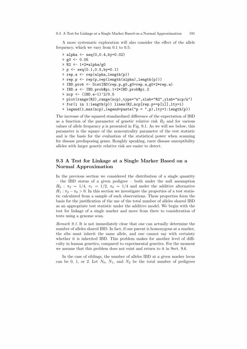
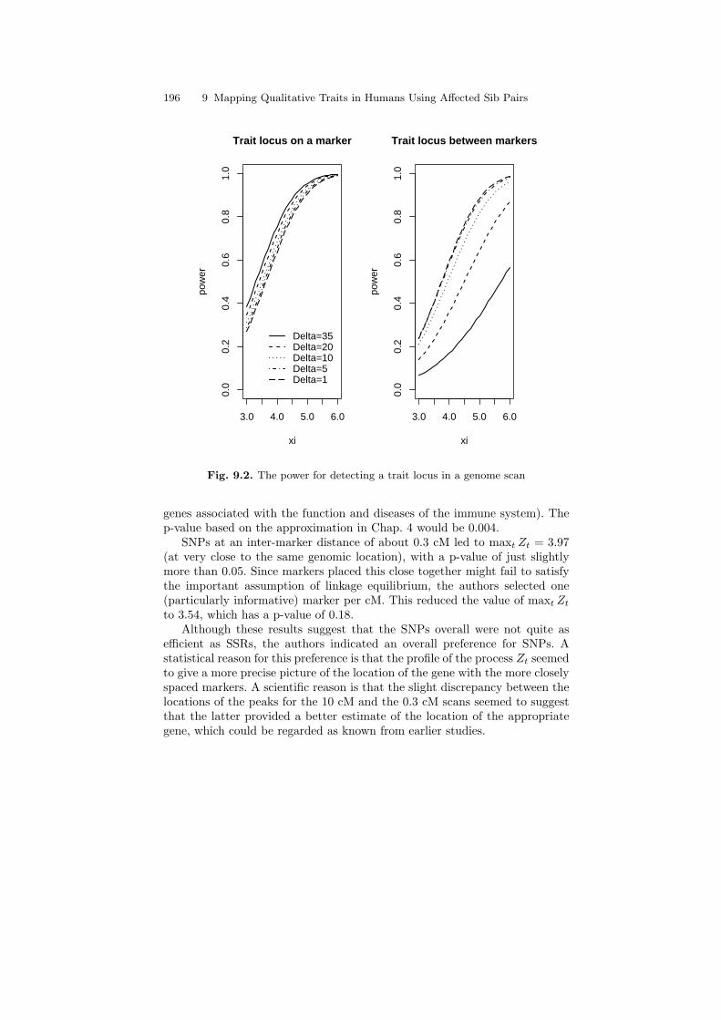
A more systematic exploration will also consider the effect of the allelefrequency, which we vary from 0.1 to 0.5:
> alpha <- seq(0,0.4,by=0.02)> g0 <- 0.05> R2 <- 1+2*alpha/g0> p <- seq(0.1,0.5,by=0.1)> rep.a <- rep(alpha,length(p))> rep.p <- rep(p,rep(length(alpha),length(p)))> IBD.prob <- DistIBD(rep.p,g0,g0+rep.a,g0+2*rep.a)> IBD.e <- IBD.prob$pi.1+2*IBD.prob$pi.2> ncp <- (IBD.e-1)^2/0.5> plot(range(R2),range(ncp),type="n",xlab="R2",ylab="ncp/n")> for(i in 1:length(p)) lines(R2,ncp[rep.p==p[i]],lty=i)> legend(1,max(ncp),legend=paste("p = ",p),lty=1:length(p))
The increase of the squared standardized difference of the expectation of IBDas a function of the parameter of genetic relative risk R2 and for variousvalues of allele frequency p is presented in Fig. 9.1. As we will see below, thisparameter is the square of the noncentrality parameter of the test statisticand is the basis for the evaluation of the statistical power when scanningfor disease predisposing genes. Roughly speaking, rarer disease susceptibilityalleles with larger genetic relative risk are easier to detect.
9.3 A Test for Linkage at a Single Marker Based on aNormal Approximation
In the previous section we considered the distribution of a single quantity– the IBD status of a given pedigree – both under the null assumptionH0 : π2 = 1/4, π1 = 1/2, π0 = 1/4 and under the additive alternativeH1 : π2 − π0 > 0. In this section we investigate the properties of a test statis-tic calculated from a sample of such observations. These properties form thebasis for the justification of the use of the total number of alleles shared IBDas an appropriate test statistic under the additive model. We begin with thetest for linkage of a single marker and move from there to consideration oftests using a genome scan.
Remark 9.1. It is not immediately clear that one can actually determine thenumber of alleles shared IBD. In fact, if one parent is homozygous at a marker,the sibs must inherit the same allele, and one cannot say with certaintywhether it is inherited IBD. This problem makes for another level of diffi-culty in human genetics, compared to experimental genetics. For the momentwe assume that this problem does not exist and return to it in Sect. 9.6.
In the case of siblings, the number of alleles IBD at a given marker locuscan be 0, 1, or 2. Let N0, N1, and N2 be the total number of pedigrees
192 9 Mapping Qualitative Traits in Humans Using Affected Sib Pairs
5 10 15
0.00
0.02
0.04
0.06
0.08
0.10
R2
ncp/
n
p = 0.1p = 0.2p = 0.3p = 0.4p = 0.5
Fig. 9.1. The squared noncentrality parameter (per unit sample size) of the IBDstatistic.
that share 0, 1, or 2 alleles IBD. The joint distribution of these counts isMultinomial(n, π), with π = (π0, π1, π2). Under the null distribution π =(1/4, 1/2, 1/4). For an additive model (i.e., σ2
D = 0) the alternative distributionat the trait locus takes the form π = (1/4−σ2
A/(8Q), 1/2, 1/4+σ2A/(8Q)). The
total IBD, standardized to have mean 0 and variance 1 under the hypothesisof no linkage, is a reasonable statistic for testing H0 : σ2
A = 0 versus thealternative H1 : σ2
A > 0.The total number of alleles shared IBD is N1 + 2N2. Since the expected
number of alleles shared IBD is n and the variance is n/2 (both computedunder the null distribution), and since n = N0 + N1 + N2, the standardizedstatistic is
Z =2N2 + N1 − n
(n/2)1/2=
N2 −N0
(n/2)1/2. (9.5)
Observe that the hypothesis tested is one sided, hence the null is rejectedfor large positive values of the test statistic. The threshold for significance isdetermined by the null distribution of the test statistic. As the sample size
9.4 Genome Scans 193
increases (n → ∞) the distribution of this test statistic resembles more andmore that of the standard normal distribution.
The mean of the test statistic under the alternative hypothesis for a markerperfectly linked to the trait locus τ is given by
ξ = E(Zτ ) = (2n)1/2(π2 − π0) = (n/2)1/2α/Q2 . (9.6)
The variance of Z is 1 − (α/Q2)2/2 ≈ 1, for local alternatives. The noncen-trality parameter at a linked marker is calculated below.
9.4 Genome Scans
For a genome scan, we use maxt Zt, where we now introduce the subscript t todenote marker location. The significance level and power can be found exactlyas in Chaps. 4 and 6, provided we use an approximation suitable for a one-sided test and the appropriate value of β. It turns out that β is 0.04, exactlytwice what it was for a backcross. The reason is that along each chromosome(one maternally inherited and the other paternally inherited), the two siblingsinvolve two meiotic events. In contrast a backcross involved only one. A moredetailed mathematical analysis follows.
To study the properties of Zt and hence to approximate the significancelevel and power of a genome scan using the results of Chaps. 4 and 6, it is help-ful to use the representation of the numerator 2N2t+N1t−n =
∑ni=1[Ji(t)−1].
This representation shows that the correlation function and mean value of thestandardized statistic Zt can be obtained directly from the correlation func-tion and mean value of each term in the numerator, namely J(t), the numberof alleles shared IBD by a sib pair at the marker t.
We first consider the case of markers that are unlinked to the trait locus.Under local alternatives, the same results for the covariance function holdat linked markers. Let J(t) be written as JM(t) + JF(t) where JM(t) is thenumber of alleles, 0 or 1, inherited by the siblings IBD from their mother atlocus t and JF(t) is the number inherited from their father. Let s be a locusat recombination distance θ from t. If JM(s) = 1, then JM(t) = 1 if and only ifboth sibs have recombinations between t and s on their maternally inheritedchromosome or neither sib does. The probability of no recombinations in thetwo maternal meioses is (1− θ)2, while the probability of two recombinationsis θ2. Thus Pr(JM(t) = 1|JM(s) = 1) = θ2 + (1 − θ)2. For future notationalconvenience, let ϕ be defined by 1−ϕ = θ2+(1−θ)2. Similar reasoning appliesto JF, so Pr(J(t) = 2|J(s) = 2) = (1−ϕ)2. By similar arguments one sees thatPr(J(t) = 1|J(s) = 2) = 2ϕ(1 − ϕ), Pr(J(t) = 1|J(s) = 1) = ϕ2 + (1 − ϕ)2,Pr(J(t) = 2|J(s) = 1) = ϕ(1 − ϕ), etc., so we obtain a 3 × 3 matrix oftransition probabilities from state J(s) = i to state J(t) = j, for i, j = 0, 1, 2.Some calculation with these probabilities leads to
E[J(t)− 1|J(s)] = (1− 2ϕ)[J(s)− 1] . (9.7)
194 9 Mapping Qualitative Traits in Humans Using Affected Sib Pairs
Multiplying by J(s) − 1 and taking expectations, we obtain the importantrelation
cov[J(t), J(s)] = (1− 2 ϕ)/2 = 2 θ(1− θ) = exp(−0.04 |s− t|)/2 ,
where the third equality in the preceding expression follows from the equationθ = [1 − exp(−0.02 |t − s|)]/2, for the recombination fraction θ in terms ofgenetic distance |t − s| in cM. We conclude by observing that the precedingconditional probabilities and the resulting covariance are exactly the same asfor x(t), the number of A alleles in an intercross design, except that θ hasbeen replaced by ϕ, which has the effect of turning the parameter 0.02 into0.04 in the exponent of the correlation coefficient.
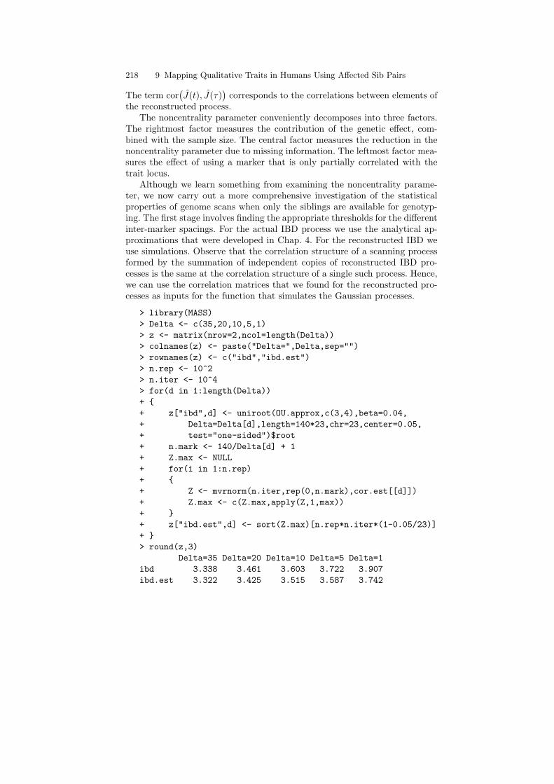
As an illustration, let us determine the thresholds for a genome scan withvarious inter-marker spacings. Note that the genetic length of the humangenome is very roughly about twice that of a mouse, or about 3,200 cM.Moreover, the genetic material in humans is distributed among 23 pairs ofchromosomes (22 pairs of autosomes and a pair of sex chromosomes). We usethese values in the approximation (??), but we divide the expression in theexponent by 2, since we are now interested in a one-sided test, and we setβ = 0.04, to obtain:
> Delta <- c(35,20,10,5,1)> z <- vector(length=length(Delta))> names(z) <- paste("Delta=",Delta,sep="")> for (i in 1:length(Delta)) z[i] <-+ uniroot(OU.approx,c(3,4),beta=0.04,Delta=Delta[i],+ length=3200,chr=23,center=0.05,test="one-sided")$root> round(z,3)Delta=35 Delta=20 Delta=10 Delta=5 Delta=1
3.337 3.459 3.601 3.721 3.906
The noncentrality parameter for a marker at no recombination distancefrom the trait locus itself was given in the preceding section. To evaluatepower in a genomic scan, we must also know the effect of recombination onthe noncentrality parameter. Observe that the reasoning behind (9.7), whichdepends only on the recombination fraction between the loci s and t continuesto apply if we set s = τ , the trait locus. By taking expectations, we concludethat at a marker t linked to the trait locus τ ,
E(Zt) = E(Zτ )(1− 2ϕ) = ξ exp(−0.04|t− τ |) .
The rate of decay of the noncentrality parameter is twice what it was for abackcross or an intercross. This means that as one increases the inter-markerdistance, there is a greater loss of power for detecting a trait locus midwaybetween markers in sib pairs than in a backcross or an intercross.
We now explore numerically the power to detect a trait locus in a genomescan as a function of the noncentrality parameter at the trait locus. We con-sider separately the case where the trait is perfectly linked to a marker and
9.4 Genome Scans 195
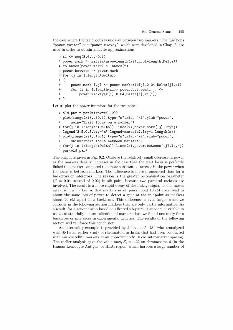
the case where the trait locus is midway between two markers. The functions“power.marker” and “power.midway”, which were developed in Chap. 6, areused in order to obtain analytic approximations:
> xi <- seq(3,6,by=0.1)> power.mark <- matrix(nrow=length(xi),ncol=length(Delta))> colnames(power.mark) <- names(z)> power.between <- power.mark> for (j in 1:length(Delta))+ {+ power.mark [,j] <- power.marker(z[j],0.04,Delta[j],xi)+ for (i in 1:length(xi)) power.between[i,j] <-+ power.midway(z[j],0.04,Delta[j],xi[i])+ }
Let us plot the power functions for the two cases:
> old.par = par(mfrow=c(1,2))> plot(range(xi),c(0,1),type="n",xlab="xi",ylab="power",+ main="Trait locus on a marker")> for(j in 1:length(Delta)) lines(xi,power.mark[,j],lty=j)> legend(3.5,0.3,bty="n",legend=names(z),lty=1:length(z))> plot(range(xi),c(0,1),type="n",xlab="xi",ylab="power",+ main="Trait locus between markers")> for(j in 1:length(Delta)) lines(xi,power.between[,j],lty=j)> par(old.par)
The output is given in Fig. 9.2. Observe the relatively small decrease in poweras the markers density increases in the case that the trait locus is perfectlylinked to a marker compared to a more substantial increase in the power whenthe locus is between markers. The difference is more pronounced than for abackcross or intercross. The reason is the greater recombination parameter(β = 0.04 instead of 0.02) in sib pairs, because two parental meioses areinvolved. The result is a more rapid decay of the linkage signal as one movesaway from a marker, so that markers in sib pairs about 10 cM apart lead toabout the same loss of power to detect a gene at the midpoint as markersabout 20 cM apart in a backcross. This difference is even larger when weconsider in the following section markers that are only partly informative. Asa result, for a genome scan based on affected sib-pairs, it appears advisable touse a substantially denser collection of markers than we found necessary for abackcross or intercross in experimental genetics. The results of the followingsection will reinforce this conclusion.
An interesting example is provided by John et al. [43], who reanalyzedwith SNPs an earlier study of rheumatoid arthritis that had been conductedwith microsatellite markers at an approximately 10 cM inter-marker spacing.The earlier analysis gave the value maxt Zt = 4.22 on chromosome 6 (in theHuman Leucocyte Antigen, or HLA, region, which harbors a large number of
196 9 Mapping Qualitative Traits in Humans Using Affected Sib Pairs
3.0 4.0 5.0 6.0
0.0
0.2
0.4
0.6
0.8
1.0
Trait locus on a marker
xi
pow
er
Delta=35Delta=20Delta=10Delta=5Delta=1
3.0 4.0 5.0 6.0
0.0
0.2
0.4
0.6
0.8
1.0
Trait locus between markers
xi
pow
er
Fig. 9.2. The power for detecting a trait locus in a genome scan
genes associated with the function and diseases of the immune system). Thep-value based on the approximation in Chap. 4 would be 0.004.
SNPs at an inter-marker distance of about 0.3 cM led to maxt Zt = 3.97(at very close to the same genomic location), with a p-value of just slightlymore than 0.05. Since markers placed this close together might fail to satisfythe important assumption of linkage equilibrium, the authors selected one(particularly informative) marker per cM. This reduced the value of maxt Zt
to 3.54, which has a p-value of 0.18.Although these results suggest that the SNPs overall were not quite as
efficient as SSRs, the authors indicated an overall preference for SNPs. Astatistical reason for this preference is that the profile of the process Zt seemedto give a more precise picture of the location of the gene with the more closelyspaced markers. A scientific reason is that the slight discrepancy between thelocations of the peaks for the 10 cM and the 0.3 cM scans seemed to suggestthat the latter provided a better estimate of the location of the appropriategene, which could be regarded as known from earlier studies.
9.5 Parametric Methods 197
9.5 Parametric Methods
The approach described above is frequently called nonparametric to distin-guish it from the parametric approach pioneered by Morton [56] and system-atically described by Ott [57]. While parameters appear in both approaches,in the parametric approach the latent genetic parameters – penetrances andallele frequencies – play an explicit role in statistics to detect linkage, whereasin the nonparametric approach one concentrates on statistical parameters,which can in principle be estimated directly from experimental data withouta specific genetic model. Examples are the frequency of a trait, or the prob-ability that a particular relative of an affected is also affected, which can beestimated from population samples of phenotypes, or noncentrality parame-ters of statistics to detect linkage, which can be estimated from a combinationof phenotypic and genotypic data. The parametric approach was developedat a time when the diseases under consideration involved a single gene, oftenshowed a clear mode of inheritance, dominant or recessive, and had essen-tially complete penetrance, so it might be reasonable to assume g0 ≈ 0, withg1 = g2 ≈ 1 for a dominant trait or g1 ≈ 0, g2 ≈ 1 for a recessive trait. More-over, the number of markers available was extremely small, so the limitingfactor in one’s ability to map a disease gene was not the genetic effect onthe trait, which was quite pronounced, but the recombination distance of thenearest marker to the gene.
For example, suppose we see the disease occurring in successive generationsof pedigrees with approximately 50% of the offspring of affected individualsalso having the disease. This suggests that the trait is dominant and fullypenetrate without sporadic cases (g0 = 0), and under an assumption of Hardy-Weinberg equilibrium we can estimate the frequency p of the disease gene fromthe population prevalence, 2p(1− p) + p2 = 2p− p2, of the trait.
The simplest illustration of a parametric analysis arises from consideringa three generation pedigree of an affected grandparent, say the grandfather,the intervening parent, say the father, and an affected grandchild. We assumethe grandmother and mother are unaffected, so under the assumption of fullpenetrance the father is also affected. Assume there is a marker that has re-combination θ with the trait, and assume that all marker alleles in the pedigreeare unique, so we know exactly which marker allele passes from the affectedgrandfather, to the father, and the allele that the father then passes to thegrandchild. If in addition to the disease allele, the father passes to his child themarker allele he received from the grandfather, then by definition there is norecombination between the disease allele and the marker allele. This happenswith probability 1 − θ. If the father passes the allele he inherited from thegrandmother, there is recombination with the disease allele, which happenswith probability θ. If we let R denote the number of recombinations, 0 or 1,we have a Bernoulli variable with Pr(R = r) = θr(1 − θ)1−r. If we have asample of n such grandchildren, the total number of recombinations in thesample would be binomial with probability θ, and we could test the hypoth-
198 9 Mapping Qualitative Traits in Humans Using Affected Sib Pairs
esis θ = 1/2 by counting these recombinations. Observe that the grandfatherand grandson share one allele IBD at the marker locus if and only if R = 0.Hence a test based on the number of recombinations is equivalently a testbased on the number of alleles shared IBD, so the parametric analysis is inthis case equivalent to a nonparametric analysis based on number of allelesshared IBD. Observe also that in this scenario there can be multiple affectedgrandchildren in a pedigree without any essential changes, and that unaffectedgrandchildren also provide linkage information. For them, however, recombi-nations have probability 1 − θ and non-recombinations have probability θ,since they are assumed not to have inherited the disease allele. Finally notethat this simple scenario would become substantially more complex if thereare sporadic cases and/or the penetrance of the disease allele is less than one,since then we could not be sure that the grandchild has the disease allele northat it comes from the grandfather. In that case an appropriate parametriclikelihood function would involve the penetrances g0, g1, g2 and the allelefrequency p in addition to θ.
Returning to the case of affected sib pairs, to put parametric and non-parametric analysis on similar footing we assume a two generation pedigree,but parental phenotypes are unknown. If there are few sporadic cases in thepopulation and the disease is rare (and dominant), we would be willing tosuppose that there is exactly one copy of the disease allele in the parentalgeneration. But we do not know which of four marker alleles present in theparents and lying on the same chromosome as the disease related locus (weassume as above that markers are completely informative) is actually linkedto the disease allele itself. (Genetic terminology is that the linkage phase isunknown.) Hence we consider the four possibilities to be equally likely. Theanalysis is more complicated but similar in principle to that given above. Itleads to the number of alleles shared IBD by the siblings, so we eventuallyarrive at the probabilities in (9.4), or more generally the corresponding prob-abilities, say πi(θ) for a marker at recombination distance θ from the diseasegene. These probabilities would be assumed known except for the parameter θ.To test the null hypothesis θ = 1/2 (no linkage) against a specific alternativevalue θ < 1/2, we could use the log likelihood ratio statistic
2∑
j=0
Nj log[πj(θ)/πj(1/2)] , (9.8)
which is often maximized with respect to θ to reflect the fact that the trueθ is almost always unknown. Under the conditions described above, the non-centrality parameter of this statistic is typically large if θ is small, but wouldbe small if the true θ is close to 1/2.
A detailed development of this approach, especially the modifications re-quired to deal with the fact that for complex diseases the allele frequenciesand penetrances are essentially never known, is beyond the scope of this book.The most important strength of a parametric approach, to which we return in
9.5 Parametric Methods 199
Chap. 11, is that, subject to being able to perform the required calculations, itgeneralizes directly to pedigrees having varying numbers and configurations ofaffecteds and to arbitrary combinations of pedigrees. This property has playedan important role in dealing with single gene traits of large penetrance, wherelarge pedigrees with multiple affecteds are common. It is less important fordealing with complex diseases, involving small penetrances where pedigreeswith large numbers of affecteds are rare.
The weakness of a parametric approach is that for complex diseases theremay be multiple genes of incomplete penetrance that may interact with eachother or with the environment, as well as non-genetic cases of the disease(g0 > 0), with the result that one has no clear idea of the number or valuesof the relevant penetrances and allele frequencies. In addition, since modernDNA analysis has made available a large number of mapped markers, theemphasis on testing an hypothesis about θ seems misplaced. We are preparedto assume that some markers are closely linked to the relevant genes. However,the complexity of the genetics can lead to small noncentrality parameters, evenat tightly linked markers, so the true signal at a linked marker may be smallcompared to the apparent signals arising from chance fluctuations at spuriousmarkers throughout the genome. Hence in our outlook we have emphasizeda null hypothesis to the effect that at the marker locus under considerationthere is effectively no departure from Mendelian segregation of genotypes, sothe noncentrality parameter of any test statistic is zero.
To gain somewhat more insight into the nature of a parametric analysis andprepare for a related discussion in Chap. 11, suppose (to simplify calculations)that δ = 0 and α is small. By using the Taylor series approximation log(1 +x) ≈ x − x2/2, valid for small |x|, one can show that the log likelihood ratiostatistic at a marker locus t assumed to be a recombination distance of θ fromthe trait locus is approximately
ξ(1− 2ϕ)Zt − ξ2(1− 2ϕ)2/2 (9.9)
where Zt is the approximately normal statistic defined above and ξ =(n/2)1/2(α/Q2) is its noncentrality at the trait locus τ . So far we have re-garded ξ as known. If we admit that it is unknown, the parameters ξ andϕ cannot be estimated separately if we only observe Zt. Only the parameterη = ξ(1− 2ϕ) can be estimated.
At this point there are different possibilities for proceeding. (i) If we max-imize the preceding expression with respect to η = ξ(1 − 2ϕ) ≥ 0, we get[max(Zt, 0)]2/2, where the nonnegativity restriction arises from the fact thatthe parameter η cannot be negative. This would be equivalent to the statisticZt (for one-sided alternatives), but as we shall see, the equivalence for thissimple problem turns out to be the exception, not the rule. (See Prob. 9.11 foran example and the related discussion in Chap. 11.) (ii) If we take the attitudethat markers are reasonably dense, so the distance from the nearest markerto the trait locus is likely to be small, we might simply set ϕ = 0 in (9.9)and scan the genome for maxima with respect to t. The result is a monotonic
200 9 Mapping Qualitative Traits in Humans Using Affected Sib Pairs
function of max Zt, hence is again equivalent to using max Zt directly. (iii) Ifwe take into consideration that we have a collection of mapped markers, thesituation is similar to that in Chap. 7. For the asymptotic Gaussian model,where the log likelihood at τ is given by (9.9) with t = τ and ϕ = 0, we canalso compute the likelihood function for a trait locus τ lying between markersti and ti+1. Using the notation of Chap. 7 (but with ϕ in place of θ), we havethat E0[Zτ |Zti
, Zti+1 ] = σ′τWZ, var0[Zτ |Zti, Zti+1 ] = 1 − σ′τWστ , and hence
the likelihood function equals
E0[exp(ξZτ − ξ2/2)|Zti , Zti+1 ] = exp(ξσ′τWZ − ξ2σ′τWστ/2) .
For ξ regarded as known, the likelihood ratio statistic for a genome scan wouldbe the maximum over τ of the expression appearing in the exponent. If ξ isregarded as unknown, we can maximize over ξ ≥ 0 as well. This leads to aone-sided version of the statistic in Chap. 7. Based on the results of Chap. 7,it seems unlikely that these statistics will be substantially more powerful thanthe simpler statistics studied earlier in this chapter.
9.6 Estimating the Number of Alleles Shared IBD
In general, IBD status, which is the basis for the statistics discussed above,is not observed directly. It needs to be inferred from genotype information.Assume that both parents of the siblings were recruited and the genotypesof all the given members of the family were obtained. If multi-allelic mark-ers are used, one may be able to observe that at a particular locus the twoparents have four distinct alleles. This favorable scenario enables the precisedetermination of the IBD status of the siblings. At the other extreme, if bothparents are homozygous, then the specific marker provides no information re-garding the IBD status of the siblings at that locus. The marker is then saidto be uninformative. There may also exist intermediate cases, e.g., where oneparent is homozygous while the other is heterozygous, or when both parentsare heterozygous for the same two alleles. Such markers are denoted partiallyinformative. However, even when a marker is partially informative or totalyuninformative, there may be other markers nearby which are either informa-tive or at least partially informative. If these markers are sufficiently close,so there is little chance of recombination, one may attempt to infer the IBDstatus at the given locus based on the genotypes at those nearby loci andthen conduct a genome scan with reconstructed IBD statistics. The problemof partial information regarding IBD relations among the affected siblingsand the need to exploit genotype information from nearby markers in orderto reconstruct the IBD becomes even more acute if the parents are not avail-able for genotyping. This is commonly the case in late onset diseases, suchas Alzheimer disease, in which the participating affected siblings are typicallyolder and are less likely to have living parents.
9.6 Estimating the Number of Alleles Shared IBD 201
Recall that markers fall into two main classes: SNPs, which are bi-allelic,and various classes of multi-allelic markers, e.g., SSRs, which often have 4–10 alleles. While SNPs are much more numerous and more easily genotyped,they are individually less informative. In most of the following we concentrateon SNPs and find that because each one by itself is relatively uninformative,there is a considerable loss of information unless they are reasonably dense.The programs are easily adapted to multi-allelic markers and show that SSRscan be more widely separated without a corresponding loss of information.
In this section we will investigate the effect of partial information regardingthe IBD relations on the statistical properties of the test statistics. We willsubstitute for the unknown IBD statistic its conditional expectation, given thegenotypic information at hand. This is similar to the case of missing genotypesthat was discussed in Chap. 7. However, the computation of the conditionalexpectation is more complex and will require application of algorithms thatwere originally developed in the context of what are called hidden Markovmodels, or HMM in short.
The section is divided into three subsections. In the first subsection wewill develop R code for the simulation of pedigrees. The HMM algorithms willbe presented in the second subsection. In the third subsection we will explorethe statistical properties of a genome scan with affected sib pairs when onlytheir genotypes are available. The tools that were developed in the first twosubsections will be used in that exploration.
9.6.1 Simulating Pedigrees
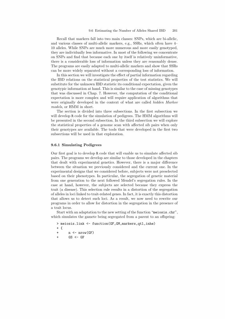
Our first goal is to develop R code that will enable us to simulate affected sibpairs. The programs we develop are similar to those developed in the chaptersthat dealt with experimental genetics. However, there is a major differencebetween the situation we previously considered and the current one. In theexperimental designs that we considered before, subjects were not preselectedbased on their phenotypes. In particular, the segregation of genetic materialfrom one generation to the next followed Mendel’s segregation rules. In thecase at hand, however, the subjects are selected because they express thetrait (a disease). This selection rule results in a distortion of the segregationof alleles in loci linked to trait-related genes. In fact, it is exactly this distortionthat allows us to detect such loci. As a result, we now need to rewrite ourprograms in order to allow for distortion in the segregation in the presence ofa trait locus.
Start with an adaptation to the new setting of the function “meiosis.chr”,which simulates the gamete being segregated from a parent to an offspring:
> meiosis.link <- function(GF,GM,markers,qtl,inhe)+ {+ n <- nrow(GF)+ GS <- GF
202 9 Mapping Qualitative Traits in Humans Using Affected Sib Pairs
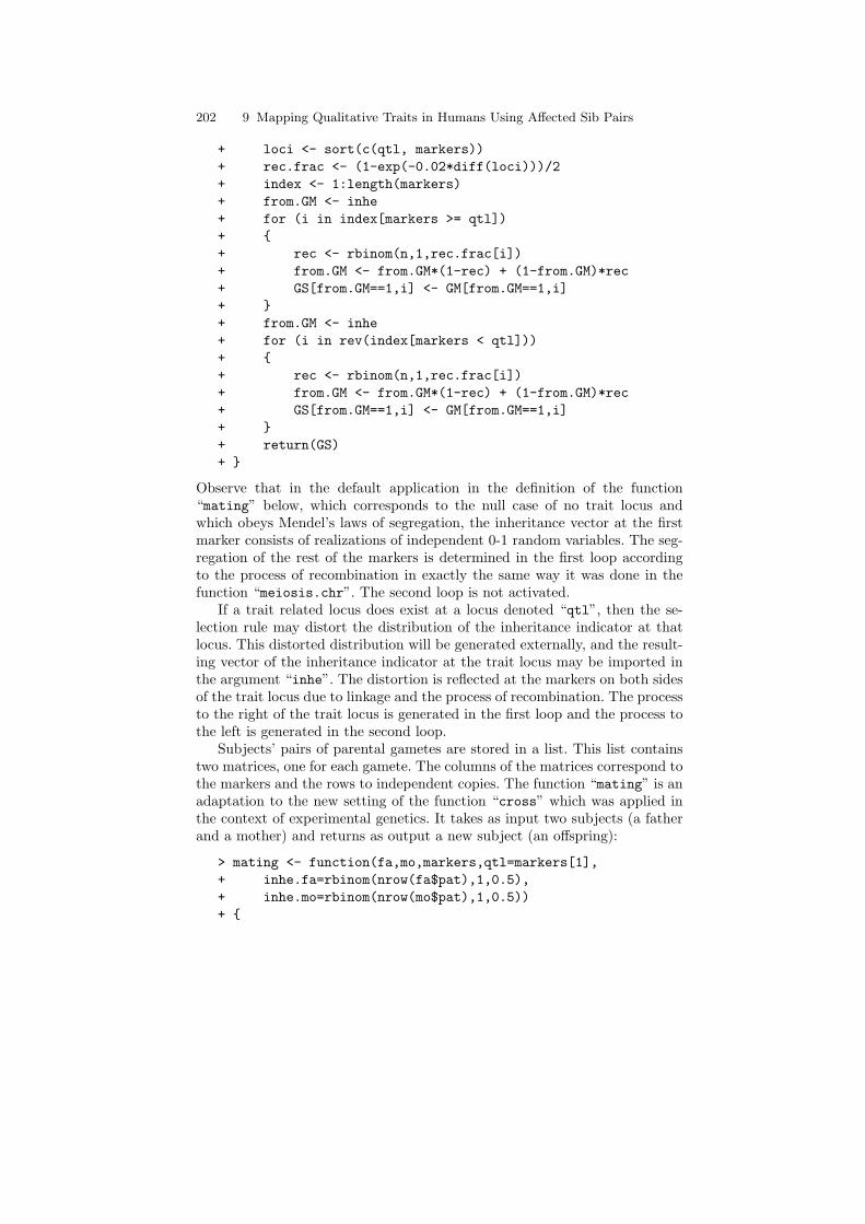
+ loci <- sort(c(qtl, markers))+ rec.frac <- (1-exp(-0.02*diff(loci)))/2+ index <- 1:length(markers)+ from.GM <- inhe+ for (i in index[markers >= qtl])+ {+ rec <- rbinom(n,1,rec.frac[i])+ from.GM <- from.GM*(1-rec) + (1-from.GM)*rec+ GS[from.GM==1,i] <- GM[from.GM==1,i]+ }+ from.GM <- inhe+ for (i in rev(index[markers < qtl]))+ {+ rec <- rbinom(n,1,rec.frac[i])+ from.GM <- from.GM*(1-rec) + (1-from.GM)*rec+ GS[from.GM==1,i] <- GM[from.GM==1,i]+ }+ return(GS)+ }
Observe that in the default application in the definition of the function“mating” below, which corresponds to the null case of no trait locus andwhich obeys Mendel’s laws of segregation, the inheritance vector at the firstmarker consists of realizations of independent 0-1 random variables. The seg-regation of the rest of the markers is determined in the first loop accordingto the process of recombination in exactly the same way it was done in thefunction “meiosis.chr”. The second loop is not activated.
If a trait related locus does exist at a locus denoted “qtl”, then the se-lection rule may distort the distribution of the inheritance indicator at thatlocus. This distorted distribution will be generated externally, and the result-ing vector of the inheritance indicator at the trait locus may be imported inthe argument “inhe”. The distortion is reflected at the markers on both sidesof the trait locus due to linkage and the process of recombination. The processto the right of the trait locus is generated in the first loop and the process tothe left is generated in the second loop.
Subjects’ pairs of parental gametes are stored in a list. This list containstwo matrices, one for each gamete. The columns of the matrices correspond tothe markers and the rows to independent copies. The function “mating” is anadaptation to the new setting of the function “cross” which was applied inthe context of experimental genetics. It takes as input two subjects (a fatherand a mother) and returns as output a new subject (an offspring):
> mating <- function(fa,mo,markers,qtl=markers[1],+ inhe.fa=rbinom(nrow(fa$pat),1,0.5),+ inhe.mo=rbinom(nrow(mo$pat),1,0.5))+ {
9.6 Estimating the Number of Alleles Shared IBD 203
+ pat <- meiosis.link(fa$pat,fa$mat,markers,qtl,inhe.fa)+ mat <- meiosis.link(mo$pat,mo$mat,markers,qtl,inhe.mo)+ return(list(pat=pat, mat=mat))+ }
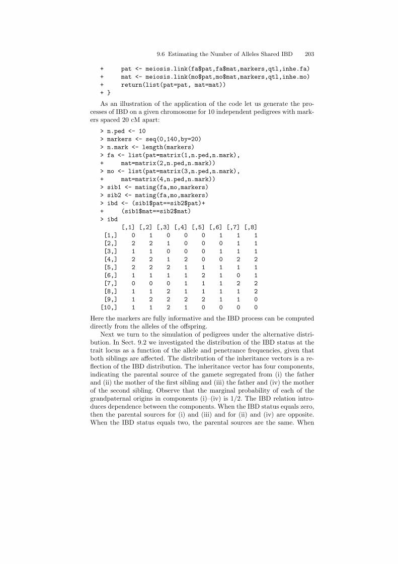
As an illustration of the application of the code let us generate the pro-cesses of IBD on a given chromosome for 10 independent pedigrees with mark-ers spaced 20 cM apart:
> n.ped <- 10> markers <- seq(0,140,by=20)> n.mark <- length(markers)> fa <- list(pat=matrix(1,n.ped,n.mark),+ mat=matrix(2,n.ped,n.mark))> mo <- list(pat=matrix(3,n.ped,n.mark),+ mat=matrix(4,n.ped,n.mark))> sib1 <- mating(fa,mo,markers)> sib2 <- mating(fa,mo,markers)> ibd <- (sib1$pat==sib2$pat)++ (sib1$mat==sib2$mat)> ibd
[,1] [,2] [,3] [,4] [,5] [,6] [,7] [,8][1,] 0 1 0 0 0 1 1 1[2,] 2 2 1 0 0 0 1 1[3,] 1 1 0 0 0 1 1 1[4,] 2 2 1 2 0 0 2 2[5,] 2 2 2 1 1 1 1 1[6,] 1 1 1 1 2 1 0 1[7,] 0 0 0 1 1 1 2 2[8,] 1 1 2 1 1 1 1 2[9,] 1 2 2 2 2 1 1 0
[10,] 1 1 2 1 0 0 0 0
Here the markers are fully informative and the IBD process can be computeddirectly from the alleles of the offspring.
Next we turn to the simulation of pedigrees under the alternative distri-bution. In Sect. 9.2 we investigated the distribution of the IBD status at thetrait locus as a function of the allele and penetrance frequencies, given thatboth siblings are affected. The distribution of the inheritance vectors is a re-flection of the IBD distribution. The inheritance vector has four components,indicating the parental source of the gamete segregated from (i) the fatherand (ii) the mother of the first sibling and (iii) the father and (iv) the motherof the second sibling. Observe that the marginal probability of each of thegrandpaternal origins in components (i)–(iv) is 1/2. The IBD relation intro-duces dependence between the components. When the IBD status equals zero,then the parental sources for (i) and (iii) and for (ii) and (iv) are opposite.When the IBD status equals two, the parental sources are the same. When
204 9 Mapping Qualitative Traits in Humans Using Affected Sib Pairs
the IBD status equals one, then for one pair the parental source is the sameand for the other it is opposite:
> inhe.vector <- function(ibd.prob,n.ped)+ {+ ibd.qtl <- sample(0:2,n.ped,replace=TRUE,prob=ibd.prob)+ sib1.pat <- rbinom(n.ped,1,0.5)+ sib1.mat <- rbinom(n.ped,1,0.5)+ pat.equal <- rbinom(n.ped,1,0.5)+ sib2.pat <- sib1.pat*pat.equal+(1-sib1.pat)*(1-pat.equal)+ sib2.mat <- sib1.mat*(1-pat.equal)+(1-sib1.mat)*pat.equal+ inhe <- cbind(sib1.pat,sib1.mat,sib2.pat,sib2.mat)+ inhe[ibd.qtl==0,3:4] <- 1-inhe[ibd.qtl==0,1:2]+ inhe[ibd.qtl==2,3:4] <- inhe[ibd.qtl==2,1:2]+ return(inhe)+ }
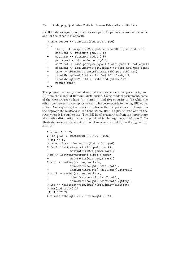
The program works by simulating first the independent components (i) and(ii) from the marginal Bernoulli distribution. Using random assignment, someof the rows are set to have (iii) match (i) and (iv) opposite to (ii) while theother rows are set in the opposite way. This corresponds to having IBD equalto one. Subsequently, the relations between the components are changed tothe appropriate relations in the rows where IBD is equal to zero and in therows where it is equal to two. The IBD itself is generated from the appropriatealternative distribution, which is provided in the argument “ibd.prob”. Toillustrate consider the additive model in which we take p = 0.2, g0 = 0.1,α = 0.4:
> n.ped <- 10^5> ibd.prob <- DistIBD(0.2,0.1,0.5,0.9)> qtl <- 80> inhe.qtl <- inhe.vector(ibd.prob,n.ped)> fa <- list(pat=matrix(1,n.ped,n.mark),+ mat=matrix(2,n.ped,n.mark))> mo <- list(pat=matrix(3,n.ped,n.mark),+ mat=matrix(4,n.ped,n.mark))> sib1 <- mating(fa, mo, markers,+ inhe.fa=inhe.qtl[,"sib1.pat"],+ inhe.mo=inhe.qtl[,"sib1.mat"],qtl=qtl)> sib2 <- mating(fa, mo, markers,+ inhe.fa=inhe.qtl[,"sib2.pat"],+ inhe.mo=inhe.qtl[,"sib2.mat"],qtl=qtl)> ibd <- (sib1$pat==sib2$pat)+(sib1$mat==sib2$mat)> sum(ibd.prob*0:2)[1] 1.137339> 2*mean(inhe.qtl[,1:2]==inhe.qtl[,3:4])
9.6 Estimating the Number of Alleles Shared IBD 205
[1] 1.1369> round(apply(ibd,2,mean),4)[1] 0.9996 1.0098 1.0261 1.0622 1.1369 1.0605 1.0288 1.0108
A susceptibility locus is present 80 cM from the telomere, next to the 5thmarker. Note that the average IBD at the marker is about equal to the expec-tation computed from the IBD probabilities. The expected IBD is elevated inthe vicinity of the trait locus and it gradually decreases to the null expectationas markers become more distant from that locus.
Now consider the replacement of the fully informative markers by par-tially informative ones. The information provided by markers is in the formof the classification of pedigrees based on the genotypes of those members forwhich the genotypes are obtained. For example, we will assume in the sequelthat genotypes are obtained for both siblings but not for their parents. Wewill also assume that the markers have n.al distinct alleles, with the defaultvalue of two. Genotype measurement for an individual returns the combinedreading of its pair of homologous chromosomes, without distinguishing theparental source. Hence, for bi-allelic markers one may obtain three distinctgenotypes. More generally, for markers with n.al alleles the total number ofdistinct genotypes is n.al(n.al+1)/2. The total number of genotypes for pairof siblings is the square of the number of individual genotypes.
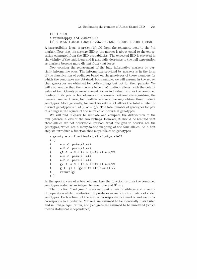
We will find it easier to simulate and compute the distribution of thefour parental alleles of the two siblings. However, it should be realized thatthese alleles are not observable. Instead, what one gets to observe are thegenotypes, which are a many-to-one mapping of the four alleles. As a firststep we introduce a function that maps alleles to genotypes:
> genotype <- function(a1,a2,a3,a4,n.al=2)+ {+ a.m <- pmin(a1,a2)+ a.M <- pmax(a1,a2)+ g1 <- a.M + (a.m-1)*(n.al-a.m/2)+ a.m <- pmin(a3,a4)+ a.M <- pmax(a3,a4)+ g2 <- a.M + (a.m-1)*(n.al-a.m/2)+ g <- g1 + (g2-1)*n.al*(n.al+1)/2+ return(g)+ }
In the specific case of a bi-allelic markers the function returns the combinedgenotypes coded as an integer between one and 32 = 9.
The function “ped.geno” takes as input a pair of siblings and a vectorof population allele distribution. It produces as an output a matrix of codedgenotypes. Each column of the matrix corresponds to a marker and each rowcorresponds to a pedigree. Markers are assumed to be identically distributedand in linkage equilibrium, and pedigrees are assumed to be unrelated (whichmeans statistical independence):
206 9 Mapping Qualitative Traits in Humans Using Affected Sib Pairs
> ped.geno <- function(sib1,sib2,f=rep(1/2,2))+ {+ n.ped <- nrow(sib1$pat)+ n.mark <- ncol(sib1$pat)+ n.al <- length(f)+ par.al <- list()+ for(par in 1:4) par.al[[par]] <-+ matrix(sample(1:n.al,n.ped*n.mark,+ replace=TRUE,prob=f),n.ped,n.mark)+ a <- inhe <- c(sib1,sib2)+ for (v in 1:4) for (par in 1:4)+ a[[v]][inhe[[v]]==par] <-+ par.al[[par]][inhe[[v]]==par]+ geno <- genotype(a[[1]],a[[2]],a[[3]],a[[4]],n.al)+ return(geno)+ }
The function works by simulating alleles (integers in the range between 1 andn.al) for each of the four parental gametes. The function “sample” is used inorder simulate the alleles from the population distribution of marker alleles.The lists “sib1” and “sib2” store two matrices each with the index of theparental source of the gamete. The resulting inherited alleles are computedand sorted in the list “a”. Finally, the function “genotype” is applied in orderto compute the resulting genotype codes.
9.6.2 Computing the Conditional Distribution of IBD
The goal in this subsection is to reconstruct the unobserved process of IBDin a pedigree using the marker genotypes. This will be conducted by thecalculation of the conditional expectation of the full-information statistic –the total number of alleles inherited IBD for the two siblings – given thegenotypic information at hand. This conditional expectation is straightforwardto compute once the conditional distribution of IBD, given the genotypes, isknown. The calculation of the latter is the subject of this subsection.
The probabilistic structure of the observations may be modeled using a“hidden” process. The hidden process is the process of IBD at the markers.This process may not be observed directly, but it does have an effect on thedistribution of the observed genotypes. This effect may be exploited in orderto make inference on the underlying hidden process. In particular, when theunderlying hidden process is Markovian and the distribution of an observa-tion is determined by the state of the hidden process at the location of theobservation, independently of its values at other locations, the model is calleda hidden Markov model (HMM). Our case fits into this setting since the pro-cess of IBD is Markovian and since markers were assumed to be in linkageequilibrium.
9.6 Estimating the Number of Alleles Shared IBD 207
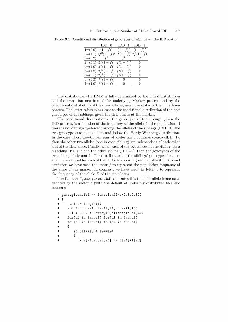
Table 9.1. Conditional distribution of genotypes of ASP, given the IBD status.
IBD=0 IBD=1 IBD=2
1=(0,0) (1− f)4 (1− f)3 (1− f)2
5=(1,1) 4f2(1− f)2 f(1− f) 2f(1− f)9=(2,2) f4 f3 f2
2=(0,1) 2f(1− f)3 f(1− f)2 04=(1,0) 2f(1− f)3 f(1− f)2 06=(1,2) 2f3(1− f) f2(1− f) 08=(2,1) 2f3(1− f) f2(1− f) 0
3=(0,2) f2(1− f)2 0 07=(2,0) f2(1− f)2 0 0
The distribution of a HMM is fully determined by the initial distributionand the transition matrices of the underlying Markov process and by theconditional distribution of the observations, given the states of the underlyingprocess. The latter refers in our case to the conditional distribution of the pairgenotypes of the siblings, given the IBD status at the marker.
The conditional distribution of the genotypes of the siblings, given theIBD process, is a function of the frequency of the alleles in the population. Ifthere is no identity-by-descent among the alleles of the siblings (IBD=0), thetwo genotypes are independent and follow the Hardy-Weinberg distribution.In the case where exactly one pair of alleles has a common source (IBD=1),then the other two alleles (one in each sibling) are independent of each otherand of the IBD allele. Finally, when each of the two alleles in one sibling has amatching IBD allele in the other sibling (IBD=2), then the genotypes of thetwo siblings fully match. The distributions of the siblings’ genotypes for a bi-allelic marker and for each of the IBD situations is given in Table 9.1. To avoidconfusion we have used the letter f to represent the population frequency ofthe allele of the marker. In contrast, we have used the letter p to representthe frequency of the allele D of the trait locus.
The function “geno.given.ibd” computes this table for allele frequenciesdenoted by the vector f (with the default of uniformly distributed bi-allelicmarker):
> geno.given.ibd <- function(f=c(0.5,0.5))+ {+ n.al <- length(f)+ P.0 <- outer(outer(f,f),outer(f,f))+ P.1 <- P.2 <- array(0,dim=rep(n.al,4))+ for(a2 in 1:n.al) for(a1 in 1:n.al)+ for(a3 in 1:n.al) for(a4 in 1:n.al)+ {+ if (a1==a3 & a2==a4)+ {+ P.2[a1,a2,a3,a4] <- f[a1]*f[a2]
208 9 Mapping Qualitative Traits in Humans Using Affected Sib Pairs
+ P.1[a1,a2,a3,a4] <- f[a1]*f[a2]*(f[a1]+f[a2])/2+ }+ if (a1==a3 & a2!=a4)+ {+ P.1[a1,a2,a3,a4] <- f[a1]*f[a2]*f[a4]/2+ }+ if (a1!=a3 & a2==a4)+ {+ P.1[a1,a2,a3,a4] <- f[a1]*f[a3]*f[a2]/2+ }+ }+ a1 <- rep(1:n.al,n.al^3)+ a2 <- rep(rep(1:n.al,rep(n.al,n.al)),n.al^2)+ a3 <- rep(rep(1:n.al,rep(n.al^2,n.al)),n.al)+ a4 <- rep(1:n.al,rep(n.al^3,n.al))+ geno <- genotype(a1,a2,a3,a4,n.al)+ P.0 <- tapply(as.vector(P.0),geno,sum)+ P.1 <- tapply(as.vector(P.1),geno,sum)+ P.2 <- tapply(as.vector(P.2),geno,sum)+ P <- cbind(P.0,P.1,P.2)+ colnames(P) <- paste("State=",0:2,sep="")+ return(P)+ }
The function works by computing the distribution of the vector of four allelesfor the two siblings in each of the IBD situations. The results are storedin three vectors, each of length n.al to the fourth power. The probabilitiesfor the different genotypes are computed by summation of the four allelicprobabilities according to the level of the genotype. This is carried out withthe aid of the function “tapply”. The function “tapply” takes as input avector, a factor, and a function. The function is applied to the collection ofvalues of the vector that correspond to each given level of the factor.
The other component is the distribution of the unobserved IBD process.This process is generated in the case under consideration as a function ofthe four inheritance indicators. Each of these indicators can be viewed asan independent process with two states (0 or 1). The states of the processesmay change from one marker to the next, depending on the recombinationfraction. Under a model of no crossover interference (the Haldane model)these independent inheritance processes are Markovian. As it turns out, forthe specific pedigree structure of two siblings the process of IBD is Markovianas well. The transition matrix of going from one marker to the next, whichwas discussed on our analysis of J in Sect. 9.3, is computed in the function“trans.mat”:
9.6 Estimating the Number of Alleles Shared IBD 209
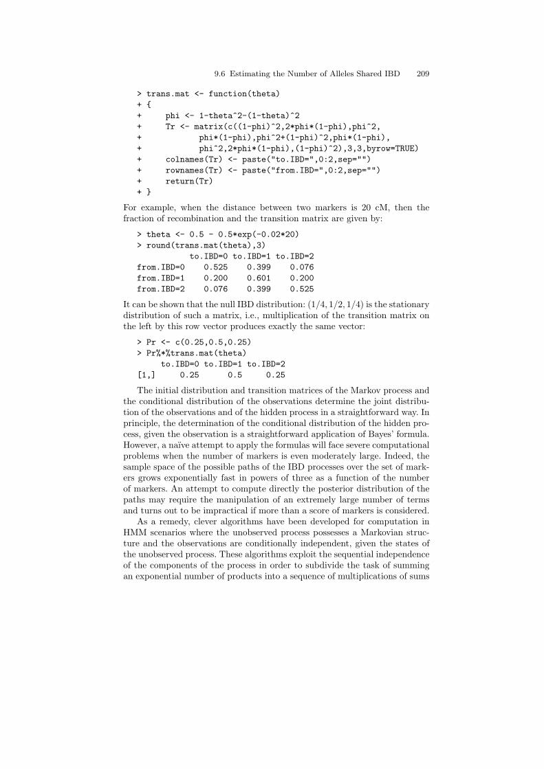
> trans.mat <- function(theta)+ {+ phi <- 1-theta^2-(1-theta)^2+ Tr <- matrix(c((1-phi)^2,2*phi*(1-phi),phi^2,+ phi*(1-phi),phi^2+(1-phi)^2,phi*(1-phi),+ phi^2,2*phi*(1-phi),(1-phi)^2),3,3,byrow=TRUE)+ colnames(Tr) <- paste("to.IBD=",0:2,sep="")+ rownames(Tr) <- paste("from.IBD=",0:2,sep="")+ return(Tr)+ }
For example, when the distance between two markers is 20 cM, then thefraction of recombination and the transition matrix are given by:
> theta <- 0.5 - 0.5*exp(-0.02*20)> round(trans.mat(theta),3)
to.IBD=0 to.IBD=1 to.IBD=2from.IBD=0 0.525 0.399 0.076from.IBD=1 0.200 0.601 0.200from.IBD=2 0.076 0.399 0.525
It can be shown that the null IBD distribution: (1/4, 1/2, 1/4) is the stationarydistribution of such a matrix, i.e., multiplication of the transition matrix onthe left by this row vector produces exactly the same vector:
> Pr <- c(0.25,0.5,0.25)> Pr%*%trans.mat(theta)
to.IBD=0 to.IBD=1 to.IBD=2[1,] 0.25 0.5 0.25
The initial distribution and transition matrices of the Markov process andthe conditional distribution of the observations determine the joint distribu-tion of the observations and of the hidden process in a straightforward way. Inprinciple, the determination of the conditional distribution of the hidden pro-cess, given the observation is a straightforward application of Bayes’ formula.However, a naıve attempt to apply the formulas will face severe computationalproblems when the number of markers is even moderately large. Indeed, thesample space of the possible paths of the IBD processes over the set of mark-ers grows exponentially fast in powers of three as a function of the numberof markers. An attempt to compute directly the posterior distribution of thepaths may require the manipulation of an extremely large number of termsand turns out to be impractical if more than a score of markers is considered.
As a remedy, clever algorithms have been developed for computation inHMM scenarios where the unobserved process possesses a Markovian struc-ture and the observations are conditionally independent, given the states ofthe unobserved process. These algorithms exploit the sequential independenceof the components of the process in order to subdivide the task of summingan exponential number of products into a sequence of multiplications of sums
210 9 Mapping Qualitative Traits in Humans Using Affected Sib Pairs
with a fixed number of summands. Below we apply two basic algorithms thatwere developed for computation in such a setting: The forward and the back-ward algorithms.
Denote by J(tm) the IBD process at the mth marker and by Pr(Gm | j)the probability of the observed genotypes at that marker, given that the IBDstatus is j. Denote the transition probability for the IBD process by Tij =Pr(J(tm) = j | J(tm−1) = i), which also equals Pr(J(tm−1) = j | J(tm) = i),since the process of recombination does not depend on the way we order themarkers, but only on the distance between them. In principle Tij will alsodepend on m when distances between markers vary. The forward algorithmcomputes recursively the quantity Fm(j) = Pr(G1, G2, . . . , Gm, J(tm) = j),which is the joint distribution of the genotypes up to locus tm and IBD statusat that locus. It does so by conditioning on the states of hidden process atthe locus tm−1 and exploiting the Markovian structure and independence inorder to obtain the relation:
Fm(j) =∑
i
Pr(G1, G2, . . . , Gm, J(tm−1) = i, J(tm) = j)
=∑
i
{Fm−1(i)× Tij × Pr(Gm | j)
}.
Summation in the relation extends over the three possible values of the IBDprocess at locus tm−1. Applying this relation recursively, starting with theinitial relation F1(j) = Pr(G1 | j)Pr(J(t1) = j), allows for the computationof these quantities for all m and j. The number of elements that needs to bemanipulated is proportional to the product of the number of markers withthe number of possible states of the underlying process (which equals three inour setting).
Denote by m the index of the last marker on the given chromosome.The backward algorithm is used in order to compute the quantity Bm(j) =Pr(Gm+1, Gm+2, . . . , Gm |J(tm) = j), namely the conditional distribution ofthe genotypes beyond a locus, given the IBD status at the locus. A recur-sive relation between the quantities can be identified. This time the relationinvolves a sum over the states of the process at tm+1 and takes the form
Bm(j) =∑
i
Pr(Gm+1, . . . , Gm, J(tm+1) = i | J(tm) = j)
=∑
i
{Bm+1(i)× Tji × Pr(Gm+1 | i)
}.
The starting values for the recursion are Bm(j) = 1.Let G = (G1, . . . , Gm) be the genetic information over the chromosome for
the given pedigree. Since Pr(G, J(tm) = j) = Pr(G1, . . . , Gm, J(tm) = j) =Fm(j)Bm(j), it follows from the definition of conditional probabilities that
Pr(J(tm) = j |G)
=Fm(j)Bm(j)∑i Fm(i)Bm(i)
. (9.10)
9.6 Estimating the Number of Alleles Shared IBD 211
Consequently, the conditional distribution of IBD, given the genotype infor-mation, can be computed at each locus as a function of the F and B quantities.
The functions “forward” and “backward” apply the forward and backwardalgorithms in order to compute the forward an backward joint distributionsof the genotypes and the IBD states. The first argument to these functions isan array “G.I” with the conditional probabilities of the observed genotypesfor each of the pedigrees, each of the markers and each of the IBD states. Thesecond and third arguments are the transition matrix of the IBD process andits initial distribution, respectively. The output are arrays that contain theforward and backward probabilities, respectively:
> forward <- function(G.I,Tr,Pr)+ {+ n.samp <- dim(G.I)[1]+ n.mark <- dim(G.I)[2]+ F <- G.I+ F[,1,] <- sweep(G.I[,1,],2,Pr,"*")+ for (i in 2:n.mark)+ {+ F[,i,] <- G.I[,i,]*(F[,i-1,]%*%Tr)+ S <- F[,i,1] + F[,i,2] + F[,i,3]+ F[,i,] <- sweep(F[,i,],1,S,"/")+ }+ return(F)+ }> backward <- function(G.I,Tr,Pr)+ {+ n.samp <- dim(G.I)[1]+ n.mark <- dim(G.I)[2]+ B <- G.I+ B[,n.mark,] <- 1+ for (i in seq(n.mark-1,1))+ {+ B[,i,] <- (G.I[,i+1,]*B[,i+1,])%*%t(Tr)+ S <- B[,i,1] + B[,i,2] + B[,i,3]+ B[,i,] <- sweep(B[,i,],1,S,"/")+ }+ return(B)+ }
Note that in each iteration of the evaluation, the currently computed quan-tities in F and B are re-scaled to sum to one. This re-scaling increases thenumerical stability of the algorithm, which would otherwise involve the ma-nipulation of terms that become vanishingly small as the algorithm progresses.Round off errors would have been a serious concern if that were the case. Ow-ing to the re-scaling, the terms are no longer the probabilities per se, but
212 9 Mapping Qualitative Traits in Humans Using Affected Sib Pairs
are only proportional to such probabilities. Nonetheless, the constants of pro-portionality do not depend on the IBD status at a locus and are thereforecanceled out of both the numerator and the denominator when (9.10) is ap-plied in order to obtain the target distribution. The actual computation ofthe conditional distribution of the states, given the genotypes, is carried outin the function “marginal.post”. This function takes as input the outputarrays of the functions “forward” and “backward” and produces an array ofthe same type with the posterior probabilities of the states:
> marginal.post <- function(F,B)+ {+ P <- F*B+ S <- P[,,1]+P[,,2]+P[,,3]+ P <- sweep(P,1:2,S,"/")+ return(P)+ }
9.6.3 Statistical Properties of Genome Scans
With the tools developed for the simulation of random pedigrees and a func-tion for the computation of the estimated identity-by-descent probabilitiesfrom the genotypic information, we can start investigating the statistical prop-erties of mapping in the more realistic setting of partial information. Let usinitiate our investigation by the determination of the expectation and covari-ance properties of the scanning statistic under both the null and the alter-native hypotheses. Later, we will consider Gaussian processes with the samecovariance and mean structure and obtain significance thresholds and powercurves. Our investigation will include several inter-marker spacings.
The first simulation is conducted under the null distribution. We simulate105 independent pedigrees and use them in order to compute the covarianceand mean structure of the reconstructed IBD process. We also assess theaccuracy of the reconstruction at a central locus. The simulation is split into100 batches in order to avoid running out of memory:
> n.rep <- 10^2> n.ped <- 10^3> Delta <- c(35,20,10,5,1)> ibd.est.null <- matrix(nrow=3,ncol=length(Delta))> colnames(ibd.est.null) <- paste("Delta=",Delta,sep="")> rownames(ibd.est.null) <- c("mean","var","mse")> cor.ibd <- vector(mode="list",length=length(Delta))> names(cor.ibd) <- paste("Delta=",Delta,sep="")> cor.est <- cor.ibd> P <- geno.given.ibd()> for(i in 1:length(Delta))
9.6 Estimating the Number of Alleles Shared IBD 213
+ {+ markers <- seq(0,140,by=Delta[i])+ n.mark <- length(markers)+ locus <- ceiling(n.mark/2)+ theta <- 0.5 - 0.5*exp(-0.02*Delta[i])+ Tr <- trans.mat(theta)+ fa <- list(pat=matrix(1,n.ped,n.mark),+ mat=matrix(2,n.ped,n.mark))+ mo <- list(pat=matrix(3,n.ped,n.mark),+ mat=matrix(4,n.ped,n.mark))+ ibd.est <- ibd <- NULL+ G.I <- array(dim=c(n.ped,n.mark,3))+ for (rep in 1:n.rep)+ {+ sib1 <- mating(fa,mo,markers)+ sib2 <- mating(fa,mo,markers)+ geno <- ped.geno(sib1,sib2)+ for(k in 1:3) G.I[,,k] <-+ matrix(P[geno,k],n.ped,n.mark)+ F.P <- forward(G.I,Tr,Pr)+ B.P <- backward(G.I,Tr,Pr)+ I.G <- marginal.post(F.P,B.P)+ ibd.est <- rbind(ibd.est,2*I.G[,,3]+I.G[,,2])+ ibd <- rbind(ibd,(sib1$pat == sib2$pat)++ (sib1$mat == sib2$mat))+ }+ ibd.est.null["mean",i] <- mean(ibd.est[,locus])+ ibd.est.null["var",i] <- var(ibd.est[,locus])+ ibd.est.null["mse",i] <-+ mean((ibd[,locus]-ibd.est[,locus])^2)+ cor.ibd[[i]] <- cor(ibd)+ cor.est[[i]] <- cor(ibd.est)+ }
Observe that mean, variance, and mean-square distance between the recon-structed and actual IBD processes are stored in a matrix called “ibd.est.null”.The columns of this matrix correspond to the different inter-marker spacings.The correlation matrices are stored in a list named “cor.est”. For later com-parison, we also store the correlation structure of the actual IBD process inthe list “cor.ibd”.
Let us examine the mean, the variance, and the quality of reconstructionunder the null distribution:
214 9 Mapping Qualitative Traits in Humans Using Affected Sib Pairs
> round(ibd.est.null,3)Delta=35 Delta=20 Delta=10 Delta=5 Delta=1
mean 1.001 1.002 1.001 1.002 0.998var 0.126 0.155 0.217 0.292 0.425mse 0.374 0.343 0.284 0.208 0.075
Several insights emerge. First, it can be seen that the expected value of theestimated IBD is about equal to the expectation of the true IBD, which is one.As a matter of fact, it can be shown mathematically that the expectations ofthe estimated and the true IBD coincide. This follows from the fact that theestimated expression is a conditional expectation and the mathematical factthat the expectation of a random variable is equal to the expectation of itsconditional expectation. (Symbolically, E(J) = E[E(J |G)].)
Second, one can conclude that the variance of the estimated IBD is lessthan the variance of the actual IBD, which is equal to 1/2. Moreover, thedenser the markers are, the closer the variance is to 1/2. Mathematically therelation between variances of the actual IBD J and the estimated IBD, whichwe denote by J , is given by the relation
var(J) = var(E(J |G)) + E(var(J |G)) = var(J) + E(var(J |G)) > var(J).
The more informative G is, the more similar J is to J and the closer theirvariances are to each other.
Third, a closer examination of the numbers in the second and third rowsreveals that their sum equals one-half – the variance of the actual IBD statistic.In mathematical terms one can express this relation in the form:
E[(J − J)2] = E[var(J |G)].
Substituted into the previous equation, this relation shows that the closer thevariance of the reconstructed IBD is to the variance of the actual IBD, themore accurate the reconstruction is, as measured by its mean squared error.
In the computation of a scanning statistic, standardization is carried outwith the standard deviation of the estimated IBD. The resulting statistic has azero mean and a unit variance under the null distribution. The Gaussian lim-iting distribution of the process of statistics is determined by the correlationstructure. In Fig. 9.3 the correlation function between a statistic computedfor a central marker and the statistics computed at the flanking markers isplotted. The spacing between markers is 10 cM. The code that produced thefigure is:
> markers <- seq(0,140,by=10)> plot(markers,cor.ibd$"Delta=10"[8,],pch=19,ylab="cor.")> points(markers,cor.est$"Delta=10"[8,])> legend(1,0.99,legend=c("Actual","Estimated"),pch=c(19,1))
The correlation values for the actual IBD process are plotted in solid blackand the values for the estimated IBD process are plotted in black and white.
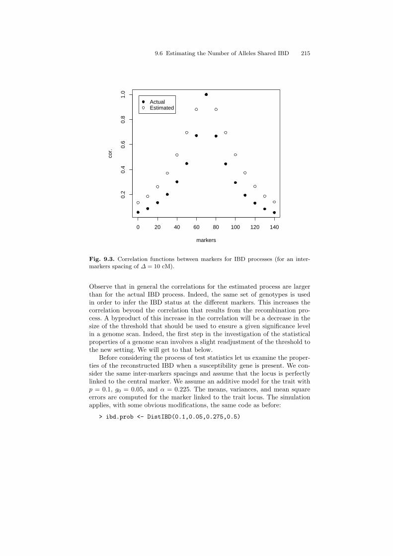
9.6 Estimating the Number of Alleles Shared IBD 215
0 20 40 60 80 100 120 140
0.2
0.4
0.6
0.8
1.0
markers
cor.
ActualEstimated
Fig. 9.3. Correlation functions between markers for IBD processes (for an inter-markers spacing of ∆ = 10 cM).
Observe that in general the correlations for the estimated process are largerthan for the actual IBD process. Indeed, the same set of genotypes is usedin order to infer the IBD status at the different markers. This increases thecorrelation beyond the correlation that results from the recombination pro-cess. A byproduct of this increase in the correlation will be a decrease in thesize of the threshold that should be used to ensure a given significance levelin a genome scan. Indeed, the first step in the investigation of the statisticalproperties of a genome scan involves a slight readjustment of the threshold tothe new setting. We will get to that below.
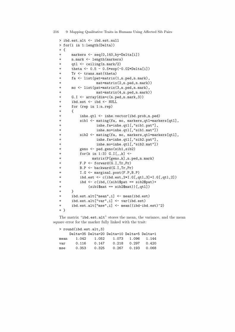
Before considering the process of test statistics let us examine the proper-ties of the reconstructed IBD when a susceptibility gene is present. We con-sider the same inter-markers spacings and assume that the locus is perfectlylinked to the central marker. We assume an additive model for the trait withp = 0.1, g0 = 0.05, and α = 0.225. The means, variances, and mean squareerrors are computed for the marker linked to the trait locus. The simulationapplies, with some obvious modifications, the same code as before:
> ibd.prob <- DistIBD(0.1,0.05,0.275,0.5)
216 9 Mapping Qualitative Traits in Humans Using Affected Sib Pairs
> ibd.est.alt <- ibd.est.null> for(i in 1:length(Delta))+ {+ markers <- seq(0,140,by=Delta[i])+ n.mark <- length(markers)+ qtl <- ceiling(n.mark/2)+ theta <- 0.5 - 0.5*exp(-0.02*Delta[i])+ Tr <- trans.mat(theta)+ fa <- list(pat=matrix(1,n.ped,n.mark),+ mat=matrix(2,n.ped,n.mark))+ mo <- list(pat=matrix(3,n.ped,n.mark),+ mat=matrix(4,n.ped,n.mark))+ G.I <- array(dim=c(n.ped,n.mark,3))+ ibd.est <- ibd <- NULL+ for (rep in 1:n.rep)+ {+ inhe.qtl <- inhe.vector(ibd.prob,n.ped)+ sib1 <- mating(fa, mo, markers,qtl=markers[qtl],+ inhe.fa=inhe.qtl[,"sib1.pat"],+ inhe.mo=inhe.qtl[,"sib1.mat"])+ sib2 <- mating(fa, mo, markers,qtl=markers[qtl],+ inhe.fa=inhe.qtl[,"sib2.pat"],+ inhe.mo=inhe.qtl[,"sib2.mat"])+ geno <- ped.geno(sib1,sib2)+ for(k in 1:3) G.I[,,k] <-+ matrix(P[geno,k],n.ped,n.mark)+ F.P <- forward(G.I,Tr,Pr)+ B.P <- backward(G.I,Tr,Pr)+ I.G <- marginal.post(F.P,B.P)+ ibd.est <- c(ibd.est,2*I.G[,qtl,3]+I.G[,qtl,2])+ ibd <- c(ibd,((sib1$pat == sib2$pat)++ (sib1$mat == sib2$mat))[,qtl])+ }+ ibd.est.alt["mean",i] <- mean(ibd.est)+ ibd.est.alt["var",i] <- var(ibd.est)+ ibd.est.alt["mse",i] <- mean((ibd-ibd.est)^2)+ }
The matrix “ibd.est.alt” stores the mean, the variance, and the meansquare error for the marker fully linked with the trait:
> round(ibd.est.alt,3)Delta=35 Delta=20 Delta=10 Delta=5 Delta=1
mean 1.042 1.052 1.073 1.096 1.144var 0.116 0.147 0.218 0.297 0.420mse 0.353 0.325 0.267 0.193 0.068
9.6 Estimating the Number of Alleles Shared IBD 217
As expected, the mean of the estimated IBD is elevated. The elevation is moreapparent when markers are denser. The variance and mean square error are,however, hardly affected by the change in distribution from unlinked to linked.This last observation is consistent with the mathematics of local alternatives,where one varies the mean but not the covariance structure.
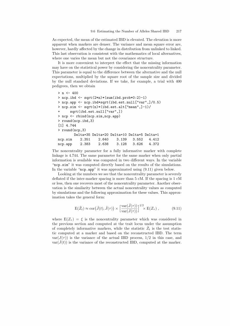
It is more convenient to interpret the effect that the missing informationmay have on the statistical power by considering the noncentrality parameter.This parameter is equal to the difference between the alternative and the nullexpectations, multiplied by the square root of the sample size and dividedby the null standard deviations. If we take, for example, a trial with 400pedigrees, then we obtain
> n <- 400> ncp.ibd <- sqrt(2*n)*(sum(ibd.prob*0:2)-1)> ncp.app <- ncp.ibd*sqrt(ibd.est.null["var",]/0.5)> ncp.sim <- sqrt(n)*(ibd.est.alt["mean",]-1)/+ sqrt(ibd.est.null["var",])> ncp <- rbind(ncp.sim,ncp.app)> round(ncp.ibd,3)[1] 4.744> round(ncp,3)
Delta=35 Delta=20 Delta=10 Delta=5 Delta=1ncp.sim 2.351 2.640 3.139 3.552 4.412ncp.app 2.383 2.638 3.128 3.626 4.372
The noncentrality parameter for a fully informative marker with completelinkage is 4.744. The same parameter for the same marker when only partialinformation is available was computed in two different ways. In the variable“ncp.sim” it was computed directly based on the results of the simulations.In the variable “ncp.app” it was approximated using (9.11) given below.
Looking at the numbers we see that the noncentrality parameter is severelydeflated if the inter-marker spacing is more than 5 cM. If the spacing is 1 cMor less, then one recovers most of the noncentrality parameter. Another obser-vation is the similarity between the actual noncentrality values as computedby simulations and the following approximation for these values. This approx-imation takes the general form:
E(Zt) ≈ cor(J(t), J(τ)
)×[var(J(τ))var(J(τ))
]1/2
× E(Zτ ) , (9.11)
where E(Zτ ) = ξ is the noncentrality parameter which was considered inthe previous section and computed at the trait locus under the assumptionof completely informative markers, while the statistic Zt is the test statis-tic computed at a marker and based on the reconstructed IBD. The termvar(J(τ)) is the variance of the actual IBD process, 1/2 in this case, andvar(J(t)) is the variance of the reconstructed IBD, computed at the marker.
218 9 Mapping Qualitative Traits in Humans Using Affected Sib Pairs
The term cor(J(t), J(τ)
)corresponds to the correlations between elements of
the reconstructed process.The noncentrality parameter conveniently decomposes into three factors.
The rightmost factor measures the contribution of the genetic effect, com-bined with the sample size. The central factor measures the reduction in thenoncentrality parameter due to missing information. The leftmost factor mea-sures the effect of using a marker that is only partially correlated with thetrait locus.
Although we learn something from examining the noncentrality parame-ter, we now carry out a more comprehensive investigation of the statisticalproperties of genome scans when only the siblings are available for genotyp-ing. The first stage involves finding the appropriate thresholds for the differentinter-marker spacings. For the actual IBD process we use the analytical ap-proximations that were developed in Chap. 4. For the reconstructed IBD weuse simulations. Observe that the correlation structure of a scanning processformed by the summation of independent copies of reconstructed IBD pro-cesses is the same at the correlation structure of a single such process. Hence,we can use the correlation matrices that we found for the reconstructed pro-cesses as inputs for the function that simulates the Gaussian processes.
> library(MASS)> Delta <- c(35,20,10,5,1)> z <- matrix(nrow=2,ncol=length(Delta))> colnames(z) <- paste("Delta=",Delta,sep="")> rownames(z) <- c("ibd","ibd.est")> n.rep <- 10^2> n.iter <- 10^4> for(d in 1:length(Delta))+ {+ z["ibd",d] <- uniroot(OU.approx,c(3,4),beta=0.04,+ Delta=Delta[d],length=140*23,chr=23,center=0.05,+ test="one-sided")$root+ n.mark <- 140/Delta[d] + 1+ Z.max <- NULL+ for(i in 1:n.rep)+ {+ Z <- mvrnorm(n.iter,rep(0,n.mark),cor.est[[d]])+ Z.max <- c(Z.max,apply(Z,1,max))+ }+ z["ibd.est",d] <- sort(Z.max)[n.rep*n.iter*(1-0.05/23)]+ }> round(z,3)
Delta=35 Delta=20 Delta=10 Delta=5 Delta=1ibd 3.338 3.461 3.603 3.722 3.907ibd.est 3.322 3.425 3.515 3.587 3.742
9.6 Estimating the Number of Alleles Shared IBD 219
As expected from our comparison of correlations, the threshold levels for thereconstructed IBD are slightly smaller than the threshold levels for the actualIBD process. We will use these lower thresholds in order to determine thepower.
For the actual IBD process we use the analytical approximation that wasdeveloped in Chapter 6. For the estimated IBD we again use simulations.Motivated by the theory of local alternatives, we simulate the process un-der the alternative distribution using the same covariance structure that wasused under the null. The mean function is computed based on the approxi-mation (9.11) and is added to each row of the random part using the function“sweep”:
> xi <- seq(3,6,by=0.1)> n.rep <- 10> power.ibd <- matrix(nrow=length(xi),ncol=length(Delta))> colnames(power.ibd) <- names(z)> power.est <- power.ibd> for (d in 1:length(Delta))+ {+ power.ibd [,d] <-+ power.marker(z["ibd",d],0.04,Delta[d],xi)+ n.mark <- 140/Delta[d] + 1+ qtl <- ceiling(n.mark/2)+ rho <- sqrt(ibd.est.null["var",d]/0.5)*+ ((cor.est[[d]])[qtl,])+ Z <- mvrnorm(n.iter,rep(0,n.mark),cor.est[[d]])+ for (i in 1:length(xi))+ {+ ncp <- xi[i]*rho+ Z1 <- sweep(Z,2,ncp,"+")+ power.est[i,d] <-+ mean(apply(Z1,1,max) >= z["ibd.est",d])+ }+ }
Let us plot the power functions:
> plot(range(xi),c(0,1),type="n",xlab="xi",ylab="power")> gr <- gray(0.75*(1:length(Delta))/length(Delta))> for(d in 1:length(Delta))+ {+ lines(xi,power.ibd[,d],col=gr[d])+ lines(xi,power.est[,d],col=gr[d],lty=2)+ }> legend(xi[1],1,bty="n",legend=colnames(z),+ lty=rep(1,ncol(z)),col=gr)
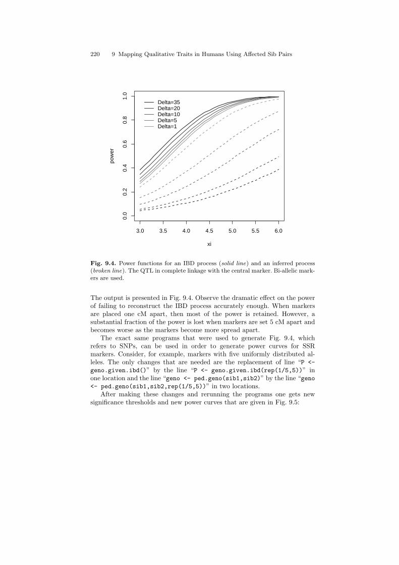
220 9 Mapping Qualitative Traits in Humans Using Affected Sib Pairs
3.0 3.5 4.0 4.5 5.0 5.5 6.0
0.0
0.2
0.4
0.6
0.8
1.0
xi
pow
er
Delta=35Delta=20Delta=10Delta=5Delta=1
Fig. 9.4. Power functions for an IBD process (solid line) and an inferred process(broken line). The QTL in complete linkage with the central marker. Bi-allelic mark-ers are used.
The output is presented in Fig. 9.4. Observe the dramatic effect on the powerof failing to reconstruct the IBD process accurately enough. When markersare placed one cM apart, then most of the power is retained. However, asubstantial fraction of the power is lost when markers are set 5 cM apart andbecomes worse as the markers become more spread apart.
The exact same programs that were used to generate Fig. 9.4, whichrefers to SNPs, can be used in order to generate power curves for SSRmarkers. Consider, for example, markers with five uniformly distributed al-leles. The only changes that are needed are the replacement of line “P <-geno.given.ibd()” by the line “P <- geno.given.ibd(rep(1/5,5))” inone location and the line “geno <- ped.geno(sib1,sib2)” by the line “geno<- ped.geno(sib1,sib2,rep(1/5,5))” in two locations.
After making these changes and rerunning the programs one gets newsignificance thresholds and new power curves that are given in Fig. 9.5:
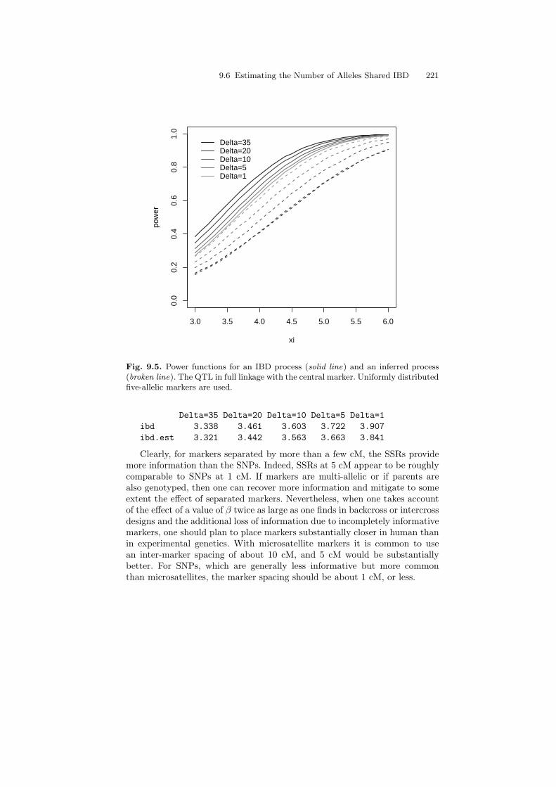
9.6 Estimating the Number of Alleles Shared IBD 221
3.0 3.5 4.0 4.5 5.0 5.5 6.0
0.0
0.2
0.4
0.6
0.8
1.0
xi
pow
er
Delta=35Delta=20Delta=10Delta=5Delta=1
Fig. 9.5. Power functions for an IBD process (solid line) and an inferred process(broken line). The QTL in full linkage with the central marker. Uniformly distributedfive-allelic markers are used.
Delta=35 Delta=20 Delta=10 Delta=5 Delta=1ibd 3.338 3.461 3.603 3.722 3.907ibd.est 3.321 3.442 3.563 3.663 3.841
Clearly, for markers separated by more than a few cM, the SSRs providemore information than the SNPs. Indeed, SSRs at 5 cM appear to be roughlycomparable to SNPs at 1 cM. If markers are multi-allelic or if parents arealso genotyped, then one can recover more information and mitigate to someextent the effect of separated markers. Nevertheless, when one takes accountof the effect of a value of β twice as large as one finds in backcross or intercrossdesigns and the additional loss of information due to incompletely informativemarkers, one should plan to place markers substantially closer in human thanin experimental genetics. With microsatellite markers it is common to usean inter-marker spacing of about 10 cM, and 5 cM would be substantiallybetter. For SNPs, which are generally less informative but more commonthan microsatellites, the marker spacing should be about 1 cM, or less.
222 9 Mapping Qualitative Traits in Humans Using Affected Sib Pairs
9.7 Bibliographical Comments
The idea of using affected sib pairs to map disease genes goes back to Pen-rose [58]. James [42] observed that the regression models used for quantitativetraits could also be used for qualitative traits if one treated the (unobserved)penetrance of a qualitative trait as a quantitative phenotype. Risch [65] pro-vided an elegant theoretical framework for single marker applications. Fordiscussion of genome scans, see Feingold, Brown, and Siegmund [28] and Lan-der and Kruglyak [48].
The standard paradigm of parametric linkage analysis is due to Mor-ton [56], and is described in detail by Ott [57].
Considerable effort has gone into the problem of reconstructing IBD re-lations from marker data. One of the first and still widely used programsfor this purpose is based on the Elston-Stewart [24] algorithm, implementedin the software SAGE. As befits its vintage, this algorithm is particularlyadept at dealing with large pedigrees and a relatively small number of mark-ers. Two widely used and freely available programs that are built around ahidden Markov model of the kind discussed in the text are GENEHUNTER(Kruglyak et al. [46]) and MERLIN (Abecassis et al. [2]). Both of these pro-grams can handle essentially any number of markers, but have problems indealing with large pedigrees. ALLEGRO [33] began its existence as somethingof an offspring of GENEHUNTER, but lately [34] seems to have developedan independent life of its own.
These programs also provide suites of statistical methods that utilize theIBD reconstruction for gene mapping. The reconstruction is computationallyintensive, so the programs should be optimized; and since the goals are reason-ably clear, one would usually want to use programs prepared by professionals.The statistical applications, on the other hand, are comparatively easy to pro-gram using available statistical software, and the appropriate methods are notso generally agreed on. Hence one might want to use the IBD reconstructionof, for example, GENEHUNTER or MERLIN as a preliminary step to one’sown statistical analysis.
Problems
9.1. (a) Plot the mean function of the Z statistic for an additive model withg0 = 0.05, for various values of p, α, and n.(b) For inter-marker spacing of ∆ = 5 cM, plot the power function for variousvalues of p, α, and n.(c) For p = 0.1 and α = 0.4, how large a value of n is required to have 90%power to detect a gene perfectly linked to a marker?
9.2. Use (9.4) to find the probabilities of IBD for an additive model withg0 = 0. Note, in particular, that these probabilities depend only on p and
9.7 Bibliographical Comments 223
not on the penetrances g1 = α, g2 = 2α. Do the same for the dominantmodel g0 = 0, g1 = g2 = α. Make numerical comparisons of the noncentralityparameters of (N2−N0)/(n/2)1/2 for the two models for different values of p.Do you find your numerical results surprising?
9.3. The probabilities of IBD for the recessive model 0 = g0 = g1 < g2 aregiven by
π0 =p2
(1 + p)2, π1 =
2p
(1 + p)2, π2 =
1(1 + p)2
,
where p is the frequency of the allele D in the population.(a) Write an R function that computes the power to detect a susceptibilitygene as a function of the relevant parameters.(b) Plot the power function for various values these parameters.
9.4. The statistic Z1 = (N2 − N0)/(n/2)1/2 is designed for an additivemodel. For a recessive model, where σ2
D À σ2A , an alternative is Z2 =
(N2 − n/4)/(3n/16)1/2.
(a) Explain why this is a reasonable statistic (for example, by calculating itsnoncentrality parameter).(b) For the additive and recessive models of the preceding two problems, forwhich g0 = 0, compare the noncentrality parameters of Z1 and Z2 as functionsof p. For which values of p does Z2 have a substantially larger noncentralityparameter than Z1? (See Chap. 11 for additional discussion of alternativestatistics when the dominance variance may be important.)
9.5. Consider the model (2.3) for the penetrance y, where e is assumed tocontain environmental effects and possibly the effect of other genes that areunlinked to the trait locus at τ . Since two siblings are expected to sharegenetic material and are also likely to share a common environment, we allowfor a covariance r = cov(e1, e2). How should the assumption (9.1) be changed?What is the effect of this generalization on (9.2) and (9.4)?
9.6. Simulate significance thresholds at various inter-marker distances whenmarkers are only partially informative and compare these thresholds to thoseobtained (either by simulation or by theoretical approximations) for fully in-formative markers. Now make similar comparisons of the power of genomescans based on the appropriate thresholds.
9.7. An alternative to the additive model, which is also particularly tractable,is the multiplicative relative risk model. The penetrances are given by g0 > 0,g1 = g0R, g2 = g0R
2, where R > 1 is called the relative risk. Assuming Hardy-Weinberg equilibrium, for a sib pair find expressions for Pr(Both affected)and the conditional probability Pr(Both affected|J(τ) = j) for j = 0, 1, 2.Generalize this model to consider two (unlinked) genes acting multiplicativelybetween loci.
224 9 Mapping Qualitative Traits in Humans Using Affected Sib Pairs
Remark 9.2. It is possible to reduce this to the canonical form given in Sect. 9.1and apply the results given in the text; but the properties of this model aresufficiently simple that one can also carry out the desired calculations fromfirst principles.
9.8. Let σ2D = 0 in (9.4). The log likelihood function for the data (N0, N1, N2)
parametrized by α/Q2 is `(α/Q2) = N2 log(1 + α/Q2) + N0 log(1 − α/Q2).Show that the statistic Z introduced in the text is the score statistic for testingthe hypothesis H0 : α = 0, which is of the form ˙(0)/{E0[ ˙(0)]2}1/2. (We usethe dot notation for derivatives. See Chap. 1 for a discussion of the scorestatistic.)
9.9. Let πi(θ) = Pr(J(t) = i|A) for a marker t at a recombination fraction θfrom a trait locus τ . Show that πi(θ) is of the same form as (9.4), but with αreplaced by α(1− 2ϕ) and δ replaced by δ(1− 2ϕ)2.
9.10. The affected sib pair method is based on the observation that affectedsibs are likely to share an excess of alleles IBD at a locus that increasessusceptibility to the trait. A sib pair of whom one affected and one unaffectedis likely to share a deficit of alleles IBD at a trait locus. Assuming there is nodominance variance, develop a model for using affected/unaffected sib pairsfor gene mapping. Find the score statistic or an otherwise reasonable statisticand evaluate its noncentrality parameter. Can you give conditions where thesesib pairs would be as useful as affected sib pairs? Does it seem plausible thatthese conditions might sometimes be satisfied?
9.11. Suppose that our sample consists of n1 affected/unaffected sib pairs, asin the preceding problem, and n2 affected sib pairs. Assuming a parametricmodel, where we regard the penetrances and allele frequencies as known, andthe validity of (9.8), propose an approximate Gaussian log likelihood ratiostatistic to combine these two kinds of sib pairs. Observe that this involves aspecific linear combination of the two Z statistics, with weights that dependon the hypothesized values of the noncentrality parameters. (This issue isdiscussed again in Chap. 11.)
9.12. Give an analysis along the lines of Sects. 9.1–9.3 for samples of (i)an affected grandparent and grandchild (ii) affected half-sibling pairs, (iii)affected first cousins pairs.
Remark 9.3. Determining the recombination parameter for first cousins in-volves a more difficult argument than the other two cases.
9.13. Compute the probability distribution of the total number of allelesshared IBD by a trio of siblings.
9.14. Show that (9.3) can be re-written in the form
E(y1y2|J) = E(y1y2) + (J − 1)α− (I{J=1} − 1/2)δ .
9.7 Bibliographical Comments 225
9.15. Recall that a trait is called recessive if δ = −α. Consider a child whoseparents are related to each other, e.g., siblings or first cousins. Let F denotethe coefficient of relatedness of the parents. Using the model (2.3) togetherwith the assumption that E(e) = 0, show that the probability the child isaffected is Q1 = m + FσD. In particular, the probability that an inbred childis affected is larger than the probability m that a child of unrelated parentsis affected. An individual is said to be homozygous by descent (HBD) at thelocus t if the two alleles at that locus are IBD. Hence the the probability ofHBD at a random locus is the coefficient of relatedness of the parents. Explainhow you could use a sample of inbred affected individuals, e.g., a sample ofaffected children of first cousins, to map a recessively acting gene. What wouldbe the noncentrality parameter at a trait locus in a large sample in terms ofthe sample size n, Q1, F , and σ2
D? How would your analysis change if youwant to consider the possibility of a second gene, which is unlinked to anddoes not interact with the first gene?