Embed Size (px)
Citation preview
Part III — Local Fields
Based on lectures by H. C. JohanssonNotes taken by Dexter Chua
Michaelmas 2016
These notes are not endorsed by the lecturers, and I have modified them (oftensignificantly) after lectures. They are nowhere near accurate representations of what
was actually lectured, and in particular, all errors are almost surely mine.
The p-adic numbers Qp (where p is any prime) were invented by Hensel in the late 19thcentury, with a view to introduce function-theoretic methods into number theory. Theyare formed by completing Q with respect to the p-adic absolute value | − |p , definedfor non-zero x ∈ Q by |x|p = p−n, where x = pna/b with a, b, n ∈ Z and a and b arecoprime to p. The p-adic absolute value allows one to study congruences modulo allpowers of p simultaneously, using analytic methods. The concept of a local field is anabstraction of the field Qp, and the theory involves an interesting blend of algebra andanalysis. Local fields provide a natural tool to attack many number-theoretic problems,and they are ubiquitous in modern algebraic number theory and arithmetic geometry.
Topics likely to be covered include:
The p-adic numbers. Local fields and their structure.
Finite extensions, Galois theory and basic ramification theory.
Polynomial equations; Hensel’s Lemma, Newton polygons.
Continuous functions on the p-adic integers, Mahler’s Theorem.
Local class field theory (time permitting).
Pre-requisites
Basic algebra, including Galois theory, and basic concepts from point set topology
and metric spaces. Some prior exposure to number fields might be useful, but is not
essential.
1
Contents III Local Fields
Contents
0 Introduction 3
1 Basic theory 41.1 Fields . . . . . . . . . . . . . . . . . . . . . . . . . . . . . . . . . 41.2 Rings . . . . . . . . . . . . . . . . . . . . . . . . . . . . . . . . . 71.3 Topological rings . . . . . . . . . . . . . . . . . . . . . . . . . . . 91.4 The p-adic numbers . . . . . . . . . . . . . . . . . . . . . . . . . 11
2 Valued fields 152.1 Hensel’s lemma . . . . . . . . . . . . . . . . . . . . . . . . . . . . 152.2 Extension of norms . . . . . . . . . . . . . . . . . . . . . . . . . . 182.3 Newton polygons . . . . . . . . . . . . . . . . . . . . . . . . . . . 22
3 Discretely valued fields 273.1 Teichmuller lifts . . . . . . . . . . . . . . . . . . . . . . . . . . . 303.2 Witt vectors* . . . . . . . . . . . . . . . . . . . . . . . . . . . . . 33
4 Some p-adic analysis 38
5 Ramification theory for local fields 435.1 Ramification index and inertia degree . . . . . . . . . . . . . . . 435.2 Unramified extensions . . . . . . . . . . . . . . . . . . . . . . . . 475.3 Totally ramified extensions . . . . . . . . . . . . . . . . . . . . . 49
6 Further ramification theory 516.1 Some filtrations . . . . . . . . . . . . . . . . . . . . . . . . . . . . 516.2 Multiple extensions . . . . . . . . . . . . . . . . . . . . . . . . . . 55
7 Local class field theory 637.1 Infinite Galois theory . . . . . . . . . . . . . . . . . . . . . . . . . 637.2 Unramified extensions and Weil group . . . . . . . . . . . . . . . 657.3 Main theorems of local class field theory . . . . . . . . . . . . . . 68
8 Lubin–Tate theory 718.1 Motivating example . . . . . . . . . . . . . . . . . . . . . . . . . 718.2 Formal groups . . . . . . . . . . . . . . . . . . . . . . . . . . . . . 758.3 Lubin–Tate extensions . . . . . . . . . . . . . . . . . . . . . . . . 79
Index 88
2
0 Introduction III Local Fields
0 Introduction
What are local fields? Suppose we are interested in some basic number theoreticproblem. Say we have a polynomial f(x1, · · · , xn) ∈ Z[x1, · · · , xn]. We want tolook for solutions a ∈ Zn, or show that there are no solutions at all. We mighttry to view this polynomial as a real polynomial, look at its roots, and see ifthey are integers. In lucky cases, we might be able to show that there are noreal solutions at all, and conclude that there cannot be any solutions at all.
On the other hand, we can try to look at it modulo some prime p. If thereare no solutions mod p, then there cannot be any solution. But sometimes p isnot enough. We might want to look at it mod p2, or p3, or . . . . One importantapplication of local fields is that we can package all these information together.In this course, we are not going to study the number theoretic problems, butjust look at the properties of the local fields for their own sake.
Throughout this course, all rings will be commutative with unity, unlessotherwise specified.
3
1 Basic theory III Local Fields
1 Basic theory
We are going to start by making loads of definitions, which you may or may nothave seen before.
1.1 Fields
Definition (Absolute value). Let K be a field. An absolute value on K is afunction | · | : K → R≥0 such that
(i) |x| = 0 iff x = 0;
(ii) |xy| = |x||y| for all x, y ∈ K;
(iii) |x+ y| ≤ |x|+ |y|.
Definition (Valued field). A valued field is a field with an absolute value.
Example. The rationals, reals and complex numbers with the usual absolutevalues are absolute values.
Example (Trivial absolute value). The trivial absolute value on a field K is theabsolute value given by
|x| =
{1 x 6= 0
0 x = 0.
The only reason we mention the trivial absolute value here is that fromnow on, we will assume that the absolute values are not trivial, because trivialabsolute values are boring and break things.
There are some familiar basic properties of the absolute value such as
Proposition. ||x| − |y|| ≤ |x − y|. Here the outer absolute value on the lefthand side is the usual absolute value of R, while the others are the absolutevalues of the relevant field.
An absolute value defines a metric d(x, y) = |x− y| on K.
Definition (Equivalence of absolute values). Let K be a field, and let | · |, | · |′be absolute values. We say they are equivalent if they induce the same topology.
Proposition. Let K be a field, and | · |, | · |′ be absolute values on K. Thenthe following are equivalent.
(i) | · | and | · |′ are equivalent
(ii) |x| < 1 implies |x|′ < 1 for all x ∈ K
(iii) There is some s ∈ R>0 such that |x|s = |x|′ for all x ∈ K.
Proof. (i) ⇒ (ii) and (iii) ⇒ (i) are easy exercises. Assume (ii), and we shallprove (iii). First observe that since |x−1| = |x|−1, we know |x| > 1 implies|x|′ > 1, and hence |x| = 1 implies |x|′ = 1. To show (iii), we have to show that
the ratio log |x|log |x′| is independent of x.
4
1 Basic theory III Local Fields
Suppose not. We may assume
log |x|log |x|′
<log |y|log |y|′
,
and moreover the logarithms are positive. Then there are m,n ∈ Z>0 such that
log |x|log |y|
<m
n<
log |x|′
log |y|′.
Then rearranging implies ∣∣∣∣ xnym∣∣∣∣ < 1 <
∣∣∣∣ xnym∣∣∣∣′ ,
a contradiction.
Exercise. Let K be a valued field. Then equivalent absolute values induce thesame the completion K of K, and K is a valued field with an absolute valueextending | · |.
In this course, we are not going to be interested in the usual absolute values.Instead, we are going to consider some really weird ones, namely non-archimedeanones.
Definition (Non-archimedean absolute value). An absolute value | · | on a fieldK is called non-archimedean if |x+ y| ≤ max(|x|, |y|). This condition is calledthe strong triangle inequality .
An absolute value which isn’t non-archimedean is called archimedean.
Metrics satisfying d(x, z) ≤ max(d(x, y), d(y, z)) are often known as ultra-metrics.
Example. Q, R and C under the usual absolute values are archimedean.
In this course, we will only consider non-archimedean absolute values. Thus,from now on, unless otherwise mentioned, an absolute value is assumed to benon-archimedean. The metric is weird!
We start by proving some absurd properties of non-archimedean absolutevalues.
Recall that the closed balls are defined by
B(x, r) = {y : |x− y| ≤ r}.
Proposition. Let (K, | · |) be a non-archimedean valued field, and let x ∈ Kand r ∈ R>0. Let z ∈ B(x, r). Then
B(x, r) = B(z, r).
So closed balls do not have unique “centers”. Every point can be viewed asthe center.
Proof. Let y ∈ B(z, r). Then
|x− y| = |(x− z) + (z − y)| ≤ max(|x− z|, |z − y|) ≤ r.
So y ∈ B(x, r). By symmetry, y ∈ B(x, r) implies y ∈ B(z, r).
5
1 Basic theory III Local Fields
Corollary. Closed balls are open.
Proof. To show that B(x, r) is open, we let z ∈ B(x, r). Then we have
{y : |y − z| < r} ⊆ B(z, r) = B(x, r).
So we know the open ball of radius r around z is contained in B(x, r). So B(x, r)is open.
Norms in non-archimedean valued fields are easy to compute:
Proposition. Let K be a non-archimedean valued field, and x, y ∈ K. If|x| > |y|, then |x+ y| = |x|.
More generally, if x =∑∞c=0 xi and the non-zero |xi| are distinct, then
|x| = max |xi|.
Proof. On the one hand, we have |x + y| ≤ max{|x|, |y|}. On the other hand,we have
|x| = |(x+ y)− y| ≤ max(|x+ y|, |y|) = |x+ y|,
since we know that we cannot have |x| ≤ |y|. So we must have |x| = |x+ y|.
Convergence is also easy for valued fields.
Proposition. Let K be a valued field.
(i) Let (xn) be a sequence in K. If xn − xn+1 → 0, then xn is Cauchy.
If we assume further that K is complete, then
(ii) Let (xn) be a sequence in K. If xn − xn+1 → 0, then a sequence (xn) inK converges.
(iii) Let∑∞n=0 yn be a series in K. If yn → 0, then
∑∞n=0 yn converges.
The converses to all these are of course also true, with the usual proofs.
Proof.
(i) Pick ε > 0 and N such that |xn − xn+1| < ε for all n ≥ N . Then givenm ≥ n ≥ N , we have
|xm − xn| = |xm − xm−1 + xm−1 − xm−2 + · · · − xn|≤ max(|xm − xm−1|, · · · , |xn+1 − xn|)< ε.
So the sequence is Cauchy.
(ii) Follows from (1) and the definition of completeness.
(iii) Follows from the definition of convergence of a series and (2).
The reason why we care about these weird non-archimedean fields is thatthey have very rich algebraic structure. In particular, there is this notion of thevaluation ring.
6
1 Basic theory III Local Fields
Definition (Valuation ring). Let K be a valued field. Then the valuation ringof K is the open subring
OK = {x : |x| ≤ 1}.
We prove that it is actually a ring
Proposition. Let K be a valued field. Then
OK = {x : |x| ≤ 1}
is an open subring of K. Moreover, for each r ∈ (0, 1], the subsets {x : |x| < r}and {x : |x| ≤ r} are open ideals of OK . Moreover, O×K = {x : |x| = 1}.
Note that this is very false for usual absolute values. For example, if we takeR with the usual absolute value, we have 1 ∈ OR, but 1 + 1 6∈ OR.
Proof. We know that these sets are open since all balls are open.To see OK is a subring, we have |1| = |−1| = 1. So 1,−1 ∈ OK . If x, y ∈ OK ,
then |x+ y| ≤ max(|x|, |y|) ≤ 1. So x+ y ∈ OK . Also, |xy| = |x||y| ≤ 1 · 1 = 1.So xy ∈ OK .
That the other sets are ideals of OK is checked in the same way.To check the units, we have x ∈ O×K ⇔ |x|, |x−1| ≤ 1⇔ |x| = |x|−1 = 1.
1.2 Rings
Definition (Integral element). Let R ⊆ S be rings and s ∈ S. We say s isintegral over R if there is some monic f ∈ R[x] such that f(s) = 0.
Example. Any r ∈ R is integral (take f(x) = x− r).
Example. Take Z ⊆ C. Then z ∈ C is integral over Z if it is an algebraicinteger (by definition of algebraic integer). For example,
√2 is an algebraic
integer, but 1√2
is not.
We would like to prove the following characterization of integral elements:
Theorem. Let R ⊆ S be rings. Then s1, · · · , sn ∈ S are all integral iffR[s1, · · · , sn] ⊆ S is a finitely-generated R-module.
Note that R[s1, · · · , sn] is by definition a finitely-generated R-algebra, butrequiring it to be finitely-generated as a module is stronger.
Here one direction is easy. It is not hard to show that if s1, · · · , sn are allintegral, then R[s1, · · · , sn] is finitely-generated. However to show the otherdirection, we need to find some clever trick to produce a monic polynomial thatkills the si.
The trick we need is the adjugate matrix we know and love from IA Vectorsand Matrices.
Definition (Adjoint/Adjugate matrix). Let A = (aij) be an n× n matrix withcoefficients in a ring R. The adjugate matrix or adjoint matrix A∗ = (a∗ij) of Ais defined by
a∗ij = (−1)i+j det(Aij),
where Aij is an (n − 1) × (n − 1) matrix obtained from A by deleting the ithcolumn and the jth row.
7
1 Basic theory III Local Fields
As we know from IA, the following property holds for the adjugate matrix:
Proposition. For any A, we have A∗A = AA∗ = det(A)I, where I is theidentity matrix.
With this, we can prove our claim:
Proof of theorem. Note that we can construct R[s1, · · · , sn] by a sequence
R ⊆ R[s1] ⊆ R[s1, s2] ⊆ · · · ⊆ R[s1, · · · , sn] ⊆ S,
and each si is integral over R[s1, · · · , sn−1]. Since the finite extension of a finiteextension is still finite, it suffices to prove it for the case n = 1, and we write sfor s1.
Suppose f(x) ∈ R[x] is monic such that f(s) = 0. If g(x) ∈ R[x], then thereis some q, r ∈ R[x] such that g(x) = f(x)q(x) + r(x) with deg r < deg f . Theng(s) = r(s). So any polynomial expression in s can be written as a polynomialexpression with degree less than deg f . So R[s] is generated by 1, s, · · · , sdeg f−1.
In the other direction, let t1, · · · , td be R-module generators of R[s1, · · · , sn].We show that in fact any element of R[s1, · · · , sn] is integral over R. Considerany element b ∈ R[s1, · · · , sn]. Then there is some aij ∈ R such that
bti =
d∑j=1
aijtj .
In matrix form, this says(bI −A)t = 0.
We now multiply by (bI −A)∗ to obtain
det(bI −A)tj = 0
for all j. Now we know 1 ∈ R. So 1 =∑cjtj for some cj ∈ R. Then we have
det(bI −A) = det(bI −A)∑
cjtj =∑
cj(det(bI −A)tj) = 0.
Since det(bI −A) is a monic polynomial in b, it follows that b is integral.
Using this characterization, the following result is obvious:
Corollary. Let R ⊆ S be rings. If s1, s2 ∈ S are integral over R, then s1 + s2
and s1s2 are integral over R. In particular, the set R ⊆ S of all elements in Sintegral over R is a ring, known as the integral closure of R in S.
Proof. If s1, s2 are integral, then R[s1, s2] is a finite extension over R. Sinces1 + s2 and s1s2 are elements of R[s1, s2], they are also integral over R.
Definition (Integrally closed). Given a ring extension R ⊆ S, we say R isintegrally closed in S if R = R.
8
1 Basic theory III Local Fields
1.3 Topological rings
Recall that we previously constructed the valuation ring OK . Since the valuedfield K itself has a topology, the valuation ring inherits a subspace topology.This is in fact a ring topology.
Definition (Topological ring). Let R be a ring. A topology on R is called aring topology if addition and multiplication are continuous maps R×R→ R. Aring with a ring topology is a topological ring.
Example. R and C with the usual topologies and usual ring structures aretopological rings.
Exercise. Let K be a valued field. Then K is a topological ring. We can seethis from the fact that the product topology on K ×K is induced by the metricd((x0, y0), (x1, y1)) = max(|x0 − x1|, |y0 − y1|).
Now if we are just randomly given a ring, there is a general way of constructinga ring topology. The idea is that we pick an ideal I and declare its elements tobe small. For example, in a valued ring, we can pick I = {x ∈ OK : |x| < 1}.Now if you are not only in I, but I2, then you are even smaller. So we have ahierarchy of small sets
I ⊇ I2 ⊇ I3 ⊇ I4 ⊇ · · ·
Now to make this a topology on R, we say that a subset U ⊆ R is open if everyx ∈ U is contained in some translation of In (for some n). In other words, weneed some y ∈ R such that
x ∈ y + In ⊆ U.
But since In is additively closed, this is equivalent to saying x+ In ⊆ U . So wemake the following definition:
Definition (I-adically open). Let R be a ring and I ⊆ R an ideal. A subsetU ⊆ R is called I-adically open if for all x ∈ U , there is some n ≥ 1 such thatx+ In ⊆ U .
Proposition. The set of all I-adically open sets form a topology on R, calledthe I-adic topology .
Note that the I-adic topology isn’t really the kind of topology we are usedto thinking about, just like the topology on a valued field is also very weird.Instead, it is a “filter” for telling us how small things are.
Proof. By definition, we have ∅ and R are open, and arbitrary unions are clearlyopen. If U, V are I-adically open, and x ∈ U ∩ V , then there are n,m such thatx+ In ⊆ U and x+ Im ⊆ V . Then x+ Imax(m,n) ⊆ U ∩ V .
Exercise. Check that the I-adic topology is a ring topology.
In the special case where I = xR, we often call the I-adic topology the x-adictopology .
Now we want to tackle the notion of completeness. We will consider the caseof I = xR for motivation, but the actual definition will be completely general.
9
1 Basic theory III Local Fields
If we pick the x-adic topology, then we are essentially declaring that we takex to be small. So intuitively, we would expect power series like
a0 + a1x+ a2x2 + a3x
3 + · · ·
to “converge”, at least if the ai are “of bounded size”. In general, the ai are“not too big” if aix
i is genuinely a member of xiR, as opposed to some silly thinglike x−i.
As in the case of analysis, we would like to think of these infinite series as asequence of partial sums
(a0, a0 + a1x, a0 + a1x+ a2x2, · · · )
Now if we denote the limit as L, then we can think of this sequence alternativelyas
(L mod I, L mod I2, L mod I3, · · · ).The key property of this sequence is that if we take L mod Ik and reduce it modIk−1, then we obtain L mod Ik−1.
In general, suppose we have a sequence
(bn ∈ R/In)∞n=1.
such that bn mod In−1 = bn−1. Then we want to say that the ring is I-adicallycomplete if every sequence satisfying this property is actually of the form
(L mod I, L mod I2, L mod I3, · · · )
for some L. Alternatively, we can take the I-adic completion to be the collectionof all such sequences, and then a space is I-adically complete it is isomorphic toits I-adic completion.
To do this, we need to build up some technical machinery. The kind ofsequences we’ve just mentioned is a special case of an inverse limit.
Definition (Inverse/projective limit). Let R1, R2, , · · · be topological rings, withcontinuous homomorphisms fn : Rn+1 → Rn.
R1 R2 R3 R4 · · ·f1 f2 f3
The inverse limit or projective limit of the Ri is the ring
lim←−Rn =
{(xn) ∈
∏n
Rn : fn(xn+1) = xn
},
with coordinate-wise addition and multiplication, together with the subspacetopology coming from the product topology of
∏Rn. This topology is known as
the inverse limit topology .
Proposition. The inverse limit topology is a ring topology.
Proof sketch. We can fit the addition and multiplication maps into diagrams
lim←−Rn × lim←−Rn lim←−Rn
∏Rn ×
∏Rn
∏Rn
10
1 Basic theory III Local Fields
By the definition of the subspace topology, it suffices to show that the correspond-ing maps on
∏Rn are continuous. By the universal property of the product, it
suffices to show that the projects∏Rn ×
∏Rn → Rm is continuous for all m.
But this map can alternatively be obtained by first projecting to Rm, then doingmultiplication in Rm, and projection is continuous. So the result follows.
It is easy to see the following universal property of the inverse limit topology:
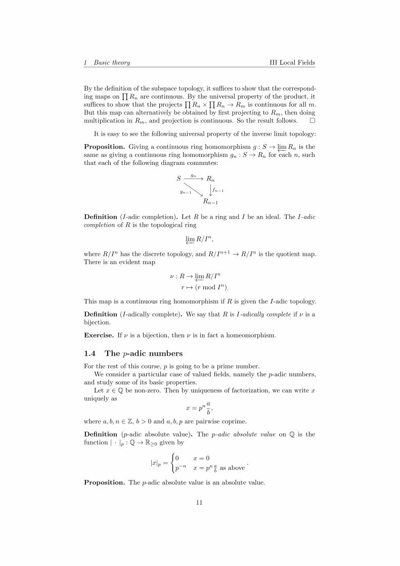
Proposition. Giving a continuous ring homomorphism g : S → lim←−Rn is thesame as giving a continuous ring homomorphism gn : S → Rn for each n, suchthat each of the following diagram commutes:
S Rn
Rn−1
gn
gn−1fn−1
Definition (I-adic completion). Let R be a ring and I be an ideal. The I-adiccompletion of R is the topological ring
lim←−R/In,
where R/In has the discrete topology, and R/In+1 → R/In is the quotient map.There is an evident map
ν : R→ lim←−R/In
r 7→ (r mod In).
This map is a continuous ring homomorphism if R is given the I-adic topology.
Definition (I-adically complete). We say that R is I-adically complete if ν is abijection.
Exercise. If ν is a bijection, then ν is in fact a homeomorphism.
1.4 The p-adic numbers
For the rest of this course, p is going to be a prime number.We consider a particular case of valued fields, namely the p-adic numbers,
and study some of its basic properties.Let x ∈ Q be non-zero. Then by uniqueness of factorization, we can write x
uniquely as
x = pna
b,
where a, b, n ∈ Z, b > 0 and a, b, p are pairwise coprime.
Definition (p-adic absolute value). The p-adic absolute value on Q is thefunction | · |p : Q→ R≥0 given by
|x|p =
{0 x = 0
p−n x = pn ab as above.
Proposition. The p-adic absolute value is an absolute value.
11
1 Basic theory III Local Fields
Proof. It is clear that |x|p = 0 iff x = 0.Suppose we have
x = pna
b, y = pm
c
d.
We wlog m ≥ n. Then we have
|xy|p =∣∣∣pn+m ac
bd
∣∣∣ = p−m−n = |x|p|y|p.
So this is multiplicative. Finally, we have
|x+ y|p =
∣∣∣∣pn ab+ pm−ncb
bd
∣∣∣∣ ≤ p−n = max(|x|p, |y|p).
Note that we must have bd coprime to p, but ab+ pm−ncb need not be. However,any extra powers of p could only decrease the absolute value, hence the aboveresult.
Note that if x ∈ Z is an integer, then |x|p = p−n iff pn || x (we say pn || x ifpn | x and pn+1 - x).
Definition (p-adic numbers). The p-adic numbers Qp is the completion of Qwith respect to | · |p.
Definition (p-adic integers). The valuation ring
Zp = {x ∈ Qp : |x|p ≤ 1}
is the p-adic integers.
Proposition. Zp is the closure of Z inside Qp.
Proof. If x ∈ Z is non-zero, then x = pna with n ≥ 0. So |x|p ≤ 1. So Z ⊆ Zp.We now want to show that Z is dense in Zp. We know the set
Z(p) = {x ∈ Q : |x|p ≤ 1}
is dense inside Zp, essentially by definition. So it suffices to show that Z is densein Z(p). We let x ∈ Z(p) \ {0}, say
x = pna
b, n ≥ 0.
It suffices to find xi ∈ Z such that xi → 1b . Then we have pnaxi → x.
Since (b, p) = 1, we can find xi, yi ∈ Z such that bxi + piyi = 1 for all i ≥ 1.So ∣∣∣∣xi − 1
b
∣∣∣∣p
=
∣∣∣∣1b∣∣∣∣p
|bxi − 1|p = |piyi|p ≤ p−i → 0.
So done.
Proposition. The non-zero ideals of Zp are pnZp for n ≥ 0. Moreover,
ZpnZ
∼=ZppnZp
.
12
1 Basic theory III Local Fields
Proof. Let 0 6= I ⊆ Zp be an ideal, and pick x ∈ I such that |x|p is maximal.This supremum exists and is attained because the possible values of the absolutevalues are discrete and bounded above. If y ∈ I, then by maximality, we have|y|p ≤ |x|p. So we have |yx−1|p ≤ 1. So yx−1 ∈ Zp, and this implies thaty = (yx−1)x ∈ xZp. So I ⊆ xZp, and we obviously have xZp ⊆ I. So we haveI = xZp.
Now if x = pn ab , then since ab is invertible in Zp, we have xZp = pnZp. So
I = pnZp.To show the second part, consider the map
fn : Z→ ZppnZp
given by the inclusion map followed by quotienting. Now pnZp = {x : |x|p ≤ p−n.So we have
ker fn = {x ∈ Z : |x|p ≤ p−n} = pnZ.
Now since Z is dense in Zp, we know the image of fn is dense in Zp/pnZp.But Zp/pnZp has the discrete topology. So fn is surjective. So fn induces anisomorphism Z/pnZ ∼= Zp/pnZp.
Corollary. Zp is a PID with a unique prime element p (up to units).
This is pretty much the point of the p-adic numbers — there are a lot ofprimes in Z, and by passing on to Zp, we are left with just one of them.
Proposition. The topology on Z induced by | · |p is the p-adic topology (i.e.the pZ-adic topology).
Proof. Let U ⊆ Z. By definition, U is open wrt | · |p iff for all x ∈ U , there isan n ∈ N such that
{y ∈ Z : |y − x|p ≤ p−n} ⊆ U.
On the other hand, U is open in the p-adic topology iff for all x ∈ U , there issome n ≥ 0 such that x+ pnZ ⊆ U . But we have
{y ∈ Z : |y − x|p ≤ p−n} = x+ pnZ.
So done.
Proposition. Zp is p-adically complete and is (isomorphic to) the p-adic com-pletion of Z.
Proof. The second part follows from the first as follows: we have the maps
Zp lim←−Zp/(pnZp) limZ/(pnZ)ν (fn)n
We know the map induced by (fn)n is an isomorphism. So we just have to showthat ν is an isomorphism
To prove the first part, we have x ∈ ker ν iff x ∈ pnZp for all n iff |x|p ≤ p−nfor all n iff |x|p = 0 iff x = 0. So the map is injective.
To show surjectivity, we let
zn ∈ lim←−Zp/pnZp.
13
1 Basic theory III Local Fields
We define ai ∈ {0, 1, · · · , p− 1} recursively such that
xn =
n−1∑i=0
aipi
is the unique representative of zn in the set of integers {0, 1, · · · , pn − 1}. Then
x =
∞∑i=0
aipi
exists in Zp and maps to x ≡ xn ≡ zn (mod pn) for all n ≥ 0. So ν(x) = (zn).So the map is surjective. So ν is bijective.
Corollary. Every a ∈ Zp has a unique expansion
a =
∞∑i=0
aipi.
with ai ∈ {0, · · · , p− 1}.More generally, for any a ∈ Q×, there is a unique expansion
a =
∞∑i=n
aipi
for ai ∈ {0, · · · , p− 1}, an 6= 0 and
n = − logp |a|p ∈ Z.
Proof. The second part follows from the first part by multiplying a by p−n.
Example. We have
1
1− p= 1 + p+ p2 + p3 + · · · .
14
2 Valued fields III Local Fields
2 Valued fields
2.1 Hensel’s lemma
We return to the discussion of general valued fields. We are now going to introducean alternative to the absolute value that contains the same information, but ispresented differently.
Definition (Valuation). Let K be a field. A valuation on K is a functionv : K → R ∪ {∞} such that
(i) v(x) = 0 iff x = 0
(ii) v(xy) = v(x) + v(y)
(iii) v(x+ y) ≥ min{v(x), v(y)}.
Here we use the conventions that r +∞ =∞ and r ≤ ∞ for all r ∈ ∞.In some sense, this definition is sort-of pointless, since if v is a valuation,
then the function|x| = c−v(x)
for any c > 1 is a (non-archimedean) absolute value. Conversely, if | · | is avaluation, then
v(x) = − logc |x|
is a valuation.Despite this, sometimes people prefer to talk about the valuation rather than
the absolute value, and often this is more natural. As we will later see, in certaincases, there is a canonical normalization of v, but there is no canonical choicefor the absolute value.
Example. For x ∈ Qp, we define
vp(x) = − logp |x|p.
This is a valuation, and if x ∈ Zp, then vp(x) = n iff pn || x.
Example. Let K be a field, and define
k((T )) =
{ ∞∑i=n
aiTi : ai ∈ k, n ∈ Z
}.
This is the field of formal Laurent series over k. We define
v(∑
aiTi)
= min{i : ai 6= 0}.
Then v is a valuation of k((T )).
Recall that for a valued field K, the valuation ring is given by
OK = {x ∈ K : |x| ≤ 1} = {x ∈ K : v(x) ≥ 0}.
Since this is a subring of a field, and the absolute value is multiplicative, wenotice that the units in O are exactly the elements of absolute value 1. The
15
2 Valued fields III Local Fields
remaining elements form an ideal (since the field is non-archimedean), and thuswe have a maximal ideal
m = mK = {x ∈ K : |x| < 1}
The quotientk = kK = OK/mK
is known as the residue field .
Example. Let K = Qp. Then O = Zp, and m = pZp. So
k = O/m = Zp/pZp ∼= Z/pZ.
Definition (Primitive polynomial). If K is a valued field and f(x) = a0 + a1x+· · ·+ anx
n ∈ K[x] is a polynomial, we say that f is primitive if
maxi|ai| = 1.
In particular, we have f ∈ O[x].
The point of a primitive polynomial is that such a polynomial is naturally,and non-trivially, an element of k[x]. Moreover, focusing on such polynomials isnot that much of a restriction, since any polynomial is a constant multiple of aprimitive polynomial.
Theorem (Hensel’s lemma). Let K be a complete valued field, and let f ∈ K[x]be primitive. Put f = f mod m ∈ k[x]. If there is a factorization
f(x) = g(x)h(x)
with (g, h) = 1, then there is a factorization
f(x) = g(x)h(x)
in O[x] withg = g, h = h mod m,
with deg g = deg g.
Note that requiring deg g = deg g is the best we can hope for — we cannotguarantee deg h = deg h, since we need not have deg f = deg f .
This is one of the most important results in the course.
Proof. Let g0, h0 be arbitrary lifts of g and h to O[x] with deg g = g0 anddeg h = h0. Then we have
f = g0h0 mod m.
The idea is to construct a “Taylor expansion” of the desired g and h term byterm, starting from g0 and h0, and using completeness to guarantee convergence.To proceed, we use our assumption that g, h are coprime to find some a, b ∈ O[x]such that
ag0 + bh0 ≡ 1 mod m. (†)
16
2 Valued fields III Local Fields
It is easier to work modulo some element π instead of modulo the ideal m, sincewe are used to doing Taylor expansion that way. Fortunately, since the equationsabove involve only finitely many coefficients, we can pick an π ∈ m with absolutevalue large enough (i.e. close enough to 1) such that the above equations holdwith m replaced with π. Thus, we can write
f = g0h0 + πr0, r0 ∈ O[x].
Plugging in (†), we get
f = g0h0 + πr0(ag0 + bh0) + π2(something).
If we are lucky enough that deg r0b < deg g0, then we group as we learnt insecondary school to get
f = (g0 + πr0b)(h0 + πr0a) + π2(something).
We can then set
g1 = g0 + πr0b
h1 = h0 + πr0a,
and then we can write
f = g1h1 + π2r1, r1 ∈ O[x], deg g1 = deg g. (∗)
If it is not true that deg r0b ≤ deg g0, we use the division algorithm to write
r0b = qg0 + p.
Then we havef = g0h0 + π((r0a+ q)g0 + ph0),
and then proceed as above.Given the factorization (∗), we replace r1 by r1(ag0 + bh0), and then repeat
the procedure to get a factorization
f ≡ g2h2 mod π3, deg g2 = deg g.
Inductively, we constrict gk, hk such that
f ≡ gkhk mod πk+1
gk ≡ gk−1 mod πk
hk ≡ hk−1 mod πk
deg gk = deg g
Note that we may drop the terms of hk whose coefficient are in πk+1O, and theabove equations still hold. Moreover, we can then bound deg hk ≤ deg f −deg gk.It now remains to set
g = limk→∞
gk, h = limk→∞
hk.
17
2 Valued fields III Local Fields
Corollary. Let f(x) = a0 + a1x+ · · ·+ anxn ∈ K[x] where K is complete and
a0, an 6= 0. If f is irreducible, then
|a`| ≤ max(|a0|, |an|)
for all `.
Proof. By scaling, we can wlog f is primitive. We then have to prove thatmax(|a0|, |an|) = 1. If not, let r be minimal such that |ar| = 1. Then 0 < r < n.Moreover, we can write
f(x) ≡ xr(ar + ar+1x+ · · ·+ anxn−r) mod m.
But then Hensel’s lemma says this lifts to a factorization of f , a contradiction.
Corollary (of Hensel’s lemma). Let f ∈ O[x] be monic, and K complete. If fmod m has a simple root α ∈ k, then f has a (unique) simple root α ∈ O liftingα.
Example. Consider xp−1 − 1 ∈ Zp[x]. We know xp−1 splits into distinct linearfactors over Fp[x]. So all roots lift to Zp. So xp−1 − 1 splits completely in Zp.So Zp contains all p roots of unity.
Example. Since 2 is a quadratic residue mod 7, we know√
2 ∈ Q7.
2.2 Extension of norms
The main goal of this section is to prove the following theorem:
Theorem. Let K be a complete valued field, and let L/K be a finite extension.Then the absolute value on K has a unique extension to an absolute value on L,given by
|α|L = n
√|NL/K(α)|,
where n = [L : K] and NL/K is the field norm. Moreover, L is complete withrespect to this absolute value.
Corollary. Let K be complete and M/K be an algebraic extension of K. Then| · | extends uniquely to an absolute value on M .
This is since any algebraic extension is the union of finite extensions, anduniqueness means we can patch the absolute values together.
Corollary. Let K be a complete valued field and L/K a finite extension. Ifσ ∈ Aut(L/K), then |σ(α)|L = |α|L.
Proof. We check that α 7→ |σ(α)|L is also an absolute value on L extending theabsolute value on K. So the result follows from uniqueness.
Before we can prove the theorem, we need some preliminaries. Given a finiteextension L/K, we would like to consider something more general than a fieldnorm on L. Instead, we will look at norms of L as a K-vector space. Thereare less axioms to check, so naturally there will be more choices for the norm.However, just as in the case of R-vector spaces, we can show that all choices ofnorms are equivalent. So to prove things about the extended field norm, oftenwe can just pick a convenient vector space norm, prove things about it, thenapply equivalence.
18
2 Valued fields III Local Fields
Definition (Norm on vector space). Let K be a valued field and V a vectorspace over K. A norm on V is a function ‖ · ‖ : V → R≥0 such that
(i) ‖x‖ = 0 iff x = 0.
(ii) ‖λ‖ = |λ| ‖x‖ for all λ ∈ K and x ∈ V .
(iii) ‖x+ y‖ ≤ max{‖x‖ , ‖y‖}.
Note that our norms are also non-Archimedean.
Definition (Equivalence of norms). Let ‖ · ‖ and ‖ · ‖′ be norms on V . Thentwo norms are equivalent if they induce the same topology on V , i.e. there areC,D > 0 such that
C ‖x‖ ≤ ‖x‖′ ≤ D ‖x‖
for all x ∈ V .
One of the most convenient norms we will work with is the max norm:
Example (Max norm). Let K be a complete valued field, and V a finite-dimensional K-vector space. Let x1, · · · , xn be a basis of V . Then if
x =∑
aixi,
then‖x‖max = max
i|ai|
defines a norm on V .
Proposition. Let K be a complete valued field, and V a finite-dimensionalK-vector space. Then V is complete under the max norm.
Proof. Given a Cauchy sequence in V under the max norm, take the limit of eachcoordinate to get the limit of the sequence, using the fact that K is complete.
That was remarkably easy. We can now immediately transfer this to all othernorms we can think of by showing all norms are equivalent.
Proposition. Let K be a complete valued field, and V a finite-dimensionalK-vector space. Then any norm ‖ · ‖ on V is equivalent to ‖ · ‖max.
Corollary. V is complete with respect to any norm.
Proof. Let ‖ · ‖ be a norm. We need to find C,D > 0 such that
C ‖x‖max ≤ ‖x‖ ≤ D ‖x‖max .
We set D = maxi(‖xi‖). Then we have
‖x‖ =∥∥∥∑ aixi
∥∥∥ ≤ max (|ai| ‖xi‖) ≤ (max |ai|)D = ‖x‖maxD.
We find C by induction on n. If n = 1, then ‖x‖ = ‖a1x1‖ = |a1| ‖x‖ =‖x‖max ‖x1‖. So C = ‖x1‖ works.
19
2 Valued fields III Local Fields
For n ≥ 2, we let
Vi = Kx1 ⊕ · · · ⊕Kxi−1 ⊕Kxi+1 ⊕ · · · ⊕Kxn= span{x1, · · · , xi−1, xi+1, · · · , xn}.
By the induction hypothesis, each Vi is complete with respect to (the restrictionof) ‖ · ‖. So in particular Vi is closed in V . So we know that the union
n⋃i=1
xi + Vi
is also closed. By construction, this does not contain 0. So there is some C > 0such that if x ∈
⋃ni=1 xi + Vi, then ‖x‖ ≥ C. We claim that
C ‖x‖max ≤ ‖x‖.
Indeed, take x =∑aixi ∈ V . Let r be such that
|ar| = maxi
(|ai|) = ‖x‖max .
Then
‖x‖−1max ‖x‖ =
∥∥a−1r x
∥∥=
∥∥∥∥a1
arx1 + · · ·+ ar−1
arxr−1 + xr +
ar+1
arxr+1 + · · ·+ an
arxn
∥∥∥∥≥ C,
since the last vector is an element of xr + Vr.
Before we can prove our theorem, we note the following two easy lemmas:
Lemma. Let K be a valued field. Then the valuation ring OK is integrallyclosed in K.
Proof. Let x ∈ K and |x| > 1. Suppose we have an−1, · · · , a0 ∈ OK . Then wehave
|xn| > |a0 + a1x+ · · ·+ an−1xn−1|.
So we knowxn + an−1x
n−1 + · · ·+ a1x+ a0
has non-zero norm, and in particular is non-zero. So x is not integral over OK .So OK is integrally closed.
Lemma. Let L be a field and | · | a function that satisfies all axioms of anabsolute value but the strong triangle inequality. Then | · | is an absolute valueiff |α| ≤ 1 implies |α+ 1| ≤ 1.
Proof. It is clear that if | · | is an absolute value, then |α| ≤ 1 implies |α+ 1| ≤ 1.Conversely, if this holds, and |x| ≤ |y|, then |x/y| ≤ 1. So |x/y + 1| ≤ 1. So
|x+ y| ≤ |y|. So |x+ y| ≤ max{|x|, |y|}.
Finally, we get to prove our theorem.
20
2 Valued fields III Local Fields
Theorem. Let K be a complete valued field, and let L/K be a finite extension.Then the absolute value on K has a unique extension to an absolute value on L,given by
|α|L = n
√∣∣NL/K(α)∣∣,
where n = [L : K] and NL/K is the field norm. Moreover, L is complete withrespect to this absolute value.
Proof. For uniqueness and completeness, if | · |L is an absolute value on L, thenit is in particular a K-norm on L as a finite-dimensional vector space. So weknow L is complete with respect to | · |L.
If | · |′L is another absolute value extending | · |, then we know | · |L and | · |′Lare equivalent in the sense of inducing the same topology. But then from one ofthe early exercises, when field norms are equivalent, then we can find some s > 0such that | · |sL = | · |′L. But the two norms agree on K, and they are non-trivial.So we must have s = 1. So the norms are equal.
To show existence, we have to prove that
|α|L = n
√∣∣NL/K(α)∣∣
is a norm.
(i) If |α|L = 0, then NL/K(α) = 0. This is true iff α = 0.
(ii) The multiplicativity of |α| and follows from the multiplicativity of NL/K ,| · | and n
√· .
To show the strong triangle inequality, it suffices to show that |α|L ≤ 1 implies|α+ 1|L ≤ 1.
Recall that
OL = {α ∈ L : |α|L ≤ 1} = {α ∈ L : NL/K(α) ∈ OK}.
We claim that OL is the integral closure of OK in L. This implies what wewant, since the integral closure is closed under addition (and 1 is in the integralclosure).
Let α ∈ OL. We may assume α 6= 0, since that case is trivial. Let theminimal polynomial of α over K be
f(x) = a0 + a1x+ · · ·+ an−1xn−1 + xn ∈ K[x].
We need to show that ai ∈ OK for all i. In other words, |ai| ≤ 1 for all i. Thisis easy for a0, since
NL/K(α) = ±am0 ,
and hence |a0| ≤ 1.By the corollary of Hensel’s lemma, for each i, we have
|ai| ≤ max(|a0|, 1)
By general properties of the field norm, there is some m ∈ Z≥1 such thatNL/K(α) = ±am0 . So we have
|ai| ≤ max(∣∣∣NL/K(α)1/m
∣∣∣ , 1) = 1.
21
2 Valued fields III Local Fields
So f ∈ OK [x]. So α is integral over OK .On the other hand, suppose α is integral over OK . Let K/K be an algebraic
closure of K. Note that
NL/K(α) =
( ∏σ:L↪→K
σ(α)
)d,
for some d ∈ Z≥1, and each σ(α) is integral over OK , since α is (apply σ to theminimal polynomial). This implies that NL/K(α) is integral over OK (and liesin K). So NL/K(α) ∈ OK since OK is integrally closed in K.
Corollary (of the proof). Let K be a complete valued field, and L/K a finiteextension. We equip L with | · |L extending | · | on K. Then OL is the integralclosure of OK in L.
2.3 Newton polygons
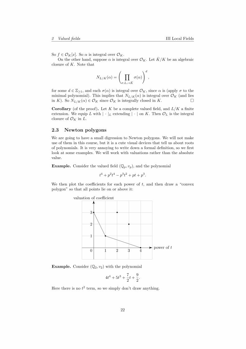
We are going to have a small digression to Newton polygons. We will not makeuse of them in this course, but it is a cute visual devices that tell us about rootsof polynomials. It is very annoying to write down a formal definition, so we firstlook at some examples. We will work with valuations rather than the absolutevalue.
Example. Consider the valued field (Qp, vp), and the polynomial
t4 + p2t4 − p3t2 + pt+ p3.
We then plot the coefficients for each power of t, and then draw a “convexpolygon” so that all points lie on or above it:
power of t
valuation of coefficient
1 2 3 40
1
2
3
Example. Consider (Q2, v2) with the polynomial
4t4 + 5t3 +7
2t+
9
2.
Here there is no t2 term, so we simply don’t draw anything.
22
2 Valued fields III Local Fields
power of t
valuation of coefficient
1 2 3 40
−1
1
2
We now go to come up with a formal definition.
Definition (Lower convex set). We say a set S ⊆ R2 is lower convex if
(i) Whenever (x, y) ∈ S, then (x, z) ∈ S for all z ≥ y.
(ii) S is convex.
Definition (Lower convex hull). Given any set of points T ⊆ R2, there is aminimal lower convex set S ⊇ T (by the intersection of all lower convex setscontaining T – this is a non-empty definition because R2 satisfies the property).This is known as the lower convex hull of the points.
Example. The lower convex hull of the points (0, 3), (1, 1), (2, 3), (3, 2), (4, 0) isgiven by the region denoted below:
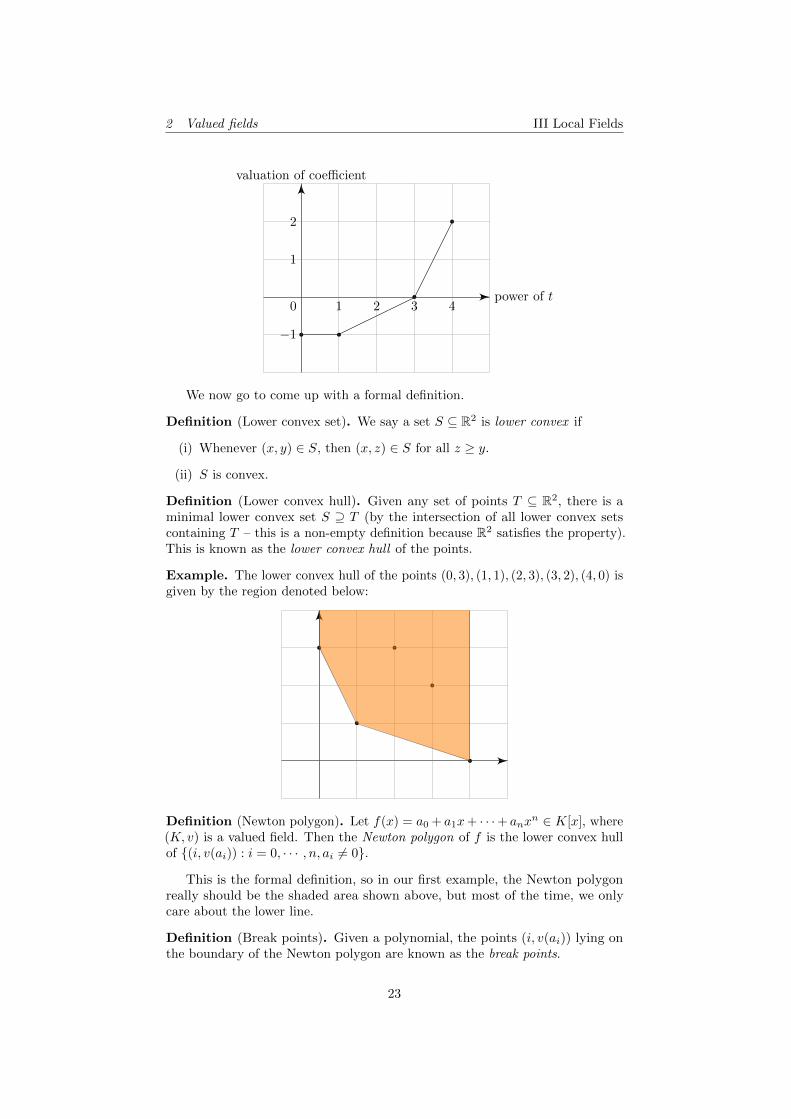
Definition (Newton polygon). Let f(x) = a0 + a1x+ · · ·+ anxn ∈ K[x], where
(K, v) is a valued field. Then the Newton polygon of f is the lower convex hullof {(i, v(ai)) : i = 0, · · · , n, ai 6= 0}.
This is the formal definition, so in our first example, the Newton polygonreally should be the shaded area shown above, but most of the time, we onlycare about the lower line.
Definition (Break points). Given a polynomial, the points (i, v(ai)) lying onthe boundary of the Newton polygon are known as the break points.
23
2 Valued fields III Local Fields
Definition (Line segment). Given a polynomial, the line segment between twoadjacent break points is a line segment .
Definition (Multiplicity/length). The length or multiplicity of a line segmentis the horizontal length.
Definition (Slope). The slope of a line segment is its slope.
Example. Consider again (Q2, v2) with the polynomial
4t4 + 5t3 +7
2t+
9
2.
power of t
valuation of coefficient
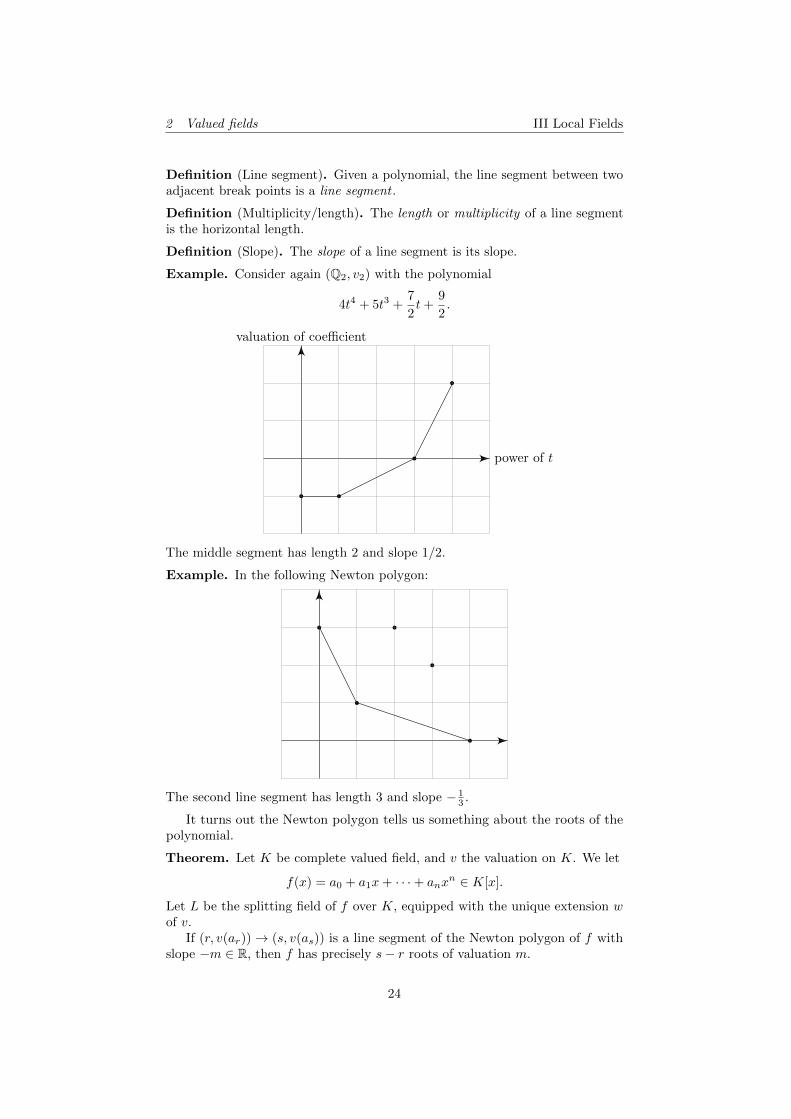
The middle segment has length 2 and slope 1/2.
Example. In the following Newton polygon:
The second line segment has length 3 and slope − 13 .
It turns out the Newton polygon tells us something about the roots of thepolynomial.
Theorem. Let K be complete valued field, and v the valuation on K. We let
f(x) = a0 + a1x+ · · ·+ anxn ∈ K[x].
Let L be the splitting field of f over K, equipped with the unique extension wof v.
If (r, v(ar))→ (s, v(as)) is a line segment of the Newton polygon of f withslope −m ∈ R, then f has precisely s− r roots of valuation m.
24
2 Valued fields III Local Fields
Note that by lower convexity, there can be at most one line segment for eachslope. So this theorem makes sense.
Proof. Dividing by an only shifts the polygon vertically, so we may wlog an = 1.We number the roots of f such that
w(α1) = · · · = w(αs1) = m1
w(αs1+1) = · · · = w(αs2) = m2
...
w(αst) = · · · = w(αn) = mt+1,
where we havem1 < m2 < · · · < mt+1.
Then we know
v(an) = v(1) = 0
v(an−1) = w(∑
αi
)≥ min
iw(αi) = m1
v(an−2) = w(∑
αiαj
)≥ min
i 6=jw(αiαj) = 2m1
...
v(an−s1) = w
∑i1 6=... 6=is1
αi1...αis1
= minw(αi1 · · ·αis1 ) = s1m1.
It is important that in the last one, we have equality, not an inequality, becausethere is one term in the sum whose valuation is less than all the others.
We can then continue to get
v(αn−s1−1) ≥ minw(αi1 · · ·αis1+1) = s1m1 +m2,
until we reachv(αn−s1−s2) = s1m1 + (s2 − s1)m2.
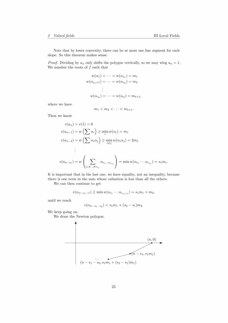
We keep going on.We draw the Newton polygon.
(n, 0)
(n− s1, s1m1)
(n− s1 − s2, s1m1 + (s2 − s1)m1)· · ·
25
2 Valued fields III Local Fields
We don’t know where exactly the other points are, but the inequalities implythat the (i, v(ai)) are above the lines drawn. So this is the Newton polygon.
Counting from the right, the first line segment has length n− (n− s1) = s1
and slope0− s1m1
n− (n− s1)= −m1.
In general, the kth segment has length (n− sk−1)− (n− sk) = sk − sk−1, andslope (
s1m1 +∑k−2i=1 (si+1 − si)mi+1
)−(s1m1 +
∑k−1i=1 (si+1 − si)mi+1
)sk − sk−1
=−(sk − sk−1)mk
sk − sk−1= −mk.
and the others follow similarly.
Corollary. If f is irreducible, then the Newton polygon has a single line segment.
Proof. We need to show that all roots have the same valuation. Let α, β be inthe splitting field L. Then there is some σ ∈ Aut(L/K) such that σ(α) = β.Then w(α) = w(σ(α)) = β. So done.
Note that Eisenstein’s criterion is a (partial) converse to this!
26
3 Discretely valued fields III Local Fields
3 Discretely valued fields
We are now going to further specialize. While a valued field already has somenice properties, we can’t really say much more about them without knowingmuch about their valuations.
Recall our previous two examples of valued fields: Qp and Fp((T )). Thevaluations had the special property that they take values in Z. Such fields areknown as discretely valued fields.
Definition (Discretely valued field). Let K be a valued field with valuation v.We say K is a discretely valued field (DVF) if v(k×) ⊆ R is a discrete subgroupof R, i.e. v(k×) is infinite cyclic.
Note that we do not require the image to be exactly Z ⊆ R. So we allowscaled versions of the valuation. This is useful because the property of mappinginto Z is not preserved under field extensions in general, as we will later see. Wewill call those that do land in Z normalized valuations.
Definition (Normalized valuation). Let K be a DVF. The normalized valuationVK on K is the unique valuation on K in the given equivalence class of valuationswhose image is Z.
Note that the normalized valuation does not give us a preferred choice ofabsolute value, since to obtain an absolute value, we still have to arbitrarily pickthe base c > 1 to define |x| = c−v(x).
Definition (Uniformizer). Let K be a discrete valued field. We say π ∈ K isuniformizer if v(π) > 0 and v(π) generates v(k×) (iff v(π) has minimal positivevaluation).
So with a normalized valuation, we have vK(π) = 1.
Example. The usual valuation on Qp is normalized, and so is the usual valuationon k((T )). p is a uniformizer for Qp and T is a uniformizer for k((T )).
The kinds of fields we will be interested are local fields. The definition wehave here might seem rather ad hoc. This is just one of the many equivalentcharacterizations of a local field, and the one we pick here is the easiest to state.
Definition (Local field). A local field is a complete discretely valued field witha finite residue field.
Example. Q and Qp with vp are both discretely valued fields, and Qp is a localfield. p is a uniformizer.
Example. The Laurent series field k((T )) with valuation
v(∑
anTn)
= inf{n : an 6= 0}
is a discrete valued field, and is a local field if and only if k is finite field, as theresidue field is exactly k. We have
Ok((T )) = k[[T ]] =
{ ∞∑n=0
anTn : an ∈ k
}.
Here T is a uniformizer.
27
3 Discretely valued fields III Local Fields
These discretely valued field are pretty much like the p-adic numbers.
Proposition. Let K be a discretely valued field with uniformizer π. Let S ⊆ OKbe a set of coset representatives of Ok/mk = kK containing 0. Then
(i) The non-zero ideals of OK are πnOK for n ≥ 0.
(ii) The ring OK is a PID with unique prime π (up to units), and mK = πOK .
(iii) The topology on OK induced by the absolute value is the π-adic topology.
(iv) If K is complete, then OK is π-adically complete.
(v) If K is complete, then any x ∈ K can be written uniquely as
x =
∞∑n�−∞
anπn,
where an ∈ S, and|x| = |π|− inf{n:an 6=0}.
(vi) The completion K is also discretely valued and π is a uniformizer, andmoreover the natural map
OkπnOk
OKπnOK
∼
is an isomorphism.
Proof. The same as for Qp and Zp, with π instead of p.
Proposition. Let K be a discretely valued field. Then K is a local field iff OKis compact.
Proof. If OK is compact, then π−nOK is compact for all n ≥ 0 (where π is theuniformizer), and in particular complete. So
K =
∞⋃n≥0
π−nOK
is complete, as this is an increasing union, and Cauchy sequences are bounded.Also, we know the quotient map OK → kK is continuous when kK is given thediscrete topology, by definition of the π-adic topology. So kK is compact anddiscrete, hence finite.
In the other direction, if K is local, then we know OK/πnOK is finite forall n ≥ 0 (by induction and finiteness of kK). We let (xi) be a sequence in OK .Then by finiteness of OK/πOK , there is a subsequence (x1,i) which is constantmodulo π. We keep going, choosing a subsequence (xn+1,i) of (xni) such that(xn+1,i) is constant modulo πn+1. Then (xi,i)
∞i=1 converges, since it is Cauchy as
|xii − xjj | ≤ |π|j
for j ≤ i. So OK is sequentially compact, hence compact.
28
3 Discretely valued fields III Local Fields
Now the valuation ring OK inherits a valuation from K, and this gives it astructure of a discrete valuation ring. We will define a discrete valuation ring ina funny way, but there are many equivalent definitions that we will not list.
Definition (Discrete valuation ring). A ring R is called a discrete valuationring (DVR) if it is a PID with a unique prime element up to units.
Proposition. R is a DVR iff R ∼= OK for some DVF K.
Proof. We have already seen that valuation rings of discrete valuation fields areDVRs. In the other direction, let R be a DVR, and π a prime. Let x ∈ R \ {0}.Then we can find a unique unit u ∈ R× and n ∈ Z≥0 such that x = πnu (say,by unique factorization of PIDs). We define
v(x) =
{n x 6= 0
∞ x = 0
This is then a discrete valuation of R. This extends uniquely to the field offractions K. It remains to show that R = OK . First note that
K = R
[1
π
].
This is since any non-zero element in R[
1π
]looks like πnu, u ∈ R×, n ∈ Z, and
is already invertible. So it must be the field of fractions. Then we have
v(πnu) = n ∈ Z≥0 ⇐⇒ πnu ∈ R.
So we have R = OK .
Now recall our two “standard” examples of valued fields — Fp((T )) andQp. Both of their residue fields are Fp, and in particular has characteristic p.However, Fp((T )) itself is also of characteristic p, while Qp has characteristic 0.It would thus be helpful to split these into two different cases:
Definition (Equal and mixed characteristic). Let K be a valued field withresidue field kK . Then K has equal characteristic if
charK = char kK .
Otherwise, we have K has mixed characteristic.
If K has mixed characteristic, then necessarily charK = 0, and char kK > 0.
Example. Qp has mixed characteristic, since charQp = 0 but char kQp =Z/pZ = p.
We will also need the following definition:
Definition (Perfect ring). Let R be a ring of characteristic p. We say R isperfect if the Frobenius map x 7→ xp is an automorphism of R, i.e. every elementof R has a pth root.
Fact. Let F be a field of characteristic p. Then F is perfect if and only if everyfinite extension of F is separable.
Example. Fq is perfect for every q = pn.
29
3 Discretely valued fields III Local Fields
3.1 Teichmuller lifts
Take our favorite discretely valued ring Zp. This is p-adically complete, so wecan write each element as
x = a0 + a1p+ a2p2 + · · · ,
where each ai is in {0, 1, · · · , p− 1}. The reason this works is that 0, 1, · · · , p−1 are coset representatives of the ring Zp/pZp ∼= Z/pZ. While these cosetrepresentatives might feel like a “natural” thing to do in this context, this isbecause we have implicitly identified with Zp/pZp ∼= Z/pZ as a particular subsetof Z ⊆ Zp. However, this identification respects effectively no algebraic structureat all. For example, we cannot multiplying the cosets simply by multiplying therepresentatives as elements of Zp, because, say, (p− 1)2 = p2 − 2p+ 1, which isnot 1. So this is actually quite bad, at least theoretically.
It turns out that we can actually construct “natural” lifts in a very generalscenario.
Theorem. Let R be a ring, and let x ∈ R. Assume that R is x-adicallycomplete and that R/xR is perfect of characteristic p. Then there is a uniquemap [−] : R/xR→ R such that
[a] ≡ a mod x
and[ab] = [a][b].
for all a, b ∈ R/xR. Moreover, if R has characteristic p, then [−] is a ringhomomorphism.
Definition (Teichmuller map). The map [−] : R/xR → R is called the Te-ichm uller map. [x] is called the Teichmuller lift or representative of x.
The idea of the proof is as follows: suppose we have an a ∈ R/xR. If werandomly picked a lift α, then chances are it would be a pretty “bad” choice,since any two such choices can differ by a multiple of x.
Suppose we instead lifted a pth root of a to R, and then take the pth powerof it. We claim that this is a better way of picking a lift. Suppose we have pickedtwo lifts of ap
−1
, say, α1 and α′1. Then α′1 = xc+ α1 for some c. So we have
(α′1)p − αp1 = αp1 + pxc+O(x2)− αp1 = pxc+O(x2),
where we abuse notation and write O(x2) to mean terms that are multiples ofx2.
We now recall that R/xR has characteristic p, so p ∈ xR. Thus in factpxc = O(x2). So we have
(α′1)p − αp1 = O(x2).
So while the lift is still arbitrary, any two arbitrary choices can differ by at mostx2. Alternatively, our lift is now a well-defined element of R/x2R.
We can, of course, do better. We can lift the p2th root of a to R, then takethe p2th power of it. Now any two lifts can differ by at most O(x3). Moregenerally, we can try to lift the pnth root of a, then take the pnth power of
30
3 Discretely valued fields III Local Fields
it. We keep picking a higher and higher n, take the limit, and hopefully getsomething useful out!
To prove this result, we will need the following messy lemma:
Lemma. Let R be a ring with x ∈ R such that R/xR has characteristic p. Letα, β ∈ R be such that
α = β mod xk (†)
Then we haveαp = βp mod xk+1.
Proof. It is left as an exercise to modify the proof to work for p = 2 (it is actuallyeasier). So suppose p is odd. We take the pth power of (†) to obtain
αp − βp +
p−1∑i=1
(p
i
)αp−iβi ∈ xp(k+1)R.
We can now write
p−1∑i=1
(−1)i(p
i
)αp−iβi =
p−12∑i=1
(−1)i(p
i
)(αβ)i
(αp−2i − βp−2i
)= p(α− β)(something).
Now since R/xR has characteristic p, we know p ∈ xR. By assumption, we knowα− β ∈ xk+1R. So this whole mess is in xk+2R, and we are done.
Proof of theorem. Let a ∈ R/xR. For each n, there is a unique ap−n ∈ R/xR.
We lift this arbitrarily to some αn ∈ R such that
αn ≡ ap−n
mod x.
We defineβn = αp
n
n .
The claim is that[a] = lim
n→∞βn
exists and is independent of the choices.Note that if the limit exists no matter how we choose the αn, then it
must be independent of the choices. Indeed, if we had choices βn and β′n,then β1, β
′2, β3, β
′4, β5, β
′6, · · · is also a respectable choice of lifts, and thus must
converge. So βn and β′n must have the same limit.Since the ring is x-adically complete and is discretely valued, to show the
limit exists, it suffices to show that βn+1 − βn → 0 x-adically. Indeed, we have
βn+1 − βn = (αpn+1)pn
− αpn
n .
We now notice that
αpn+1 ≡ (ap−n−1
)p = ap−n≡ αn mod x.
So by applying the previous the lemma many times, we obtain
(αpn+1)pn
≡ αpn
n mod xn+1.
31
3 Discretely valued fields III Local Fields
So βn+1 − βn ∈ xn+1R. So limβn exists.To see [a] = a mod x, we just have to note that
limn→∞
αpn
n ≡ limn→∞
(ap−n
)pn
= lim a = a mod x.
(here we are using the fact that the map R → R/xR is continuous when R isgiven the x-adic topology and R/xR is given the discrete topology)
The remaining properties then follow trivially from the uniqueness of theabove limit.
For multiplicativity, if we have another element b ∈ R/xR, with γn ∈ R
lifting bp−n
for all n, then αnγn lifts (ab)p−n
. So
[ab] = limαpn
n γpn
n = limαpn
n lim γpn
n = [a][b].
If R has characteristic p, then αn + γn lifts ap−n
+ bp−n
= (a+ b)p−n
. So
[a+ b] = lim(αn + γn)pn
= limαpn
n + lim γpn
n = [a] + [b].
Since 1 is a lift of 1 and 0 is a lift of 0, it follows that this is a ring homomorphism.Finally, to show uniqueness, suppose φ : R/xR → R is a map with these
properties. Then we note that φ(ap−n
) ≡ ap−n mod x, and is thus a valid choiceof αn. So we have
[a] = limn→∞
φ(ap−n
)pn
= limφ(a) = φ(a).
Example. Let R = Zp and x = p. Then [−] : Fp → Zp satisfies
[x]p−1 = [xp−1] = [1] = 1.
So the image of [x] must be the unique p− 1th root of unity lifting x (recall weproved their existence via Hensel’s lemma).
When proving theorems about these rings, the Teichmuller lifts would bevery handy and natural things to use. However, when we want to do actualcomputations, there is absolutely no reason why these would be easier!
As an application, we can prove the following characterization of equalcharacteristic complete DVF’s.
Theorem. Let K be a complete discretely valued field of equal characteristic p,and assume that kK is perfect. Then K ∼= kK((T )).
Proof. Let K be a complete DVF. Since every DVF the field of fractions ofits valuation ring, it suffices to prove that OK ∼= kK [[T ]]. We know OK hascharacteristic p. So [−] : kK → OK is an injective ring homomorphism. Wechoose a uniformizer π ∈ OK , and define
kK [[T ]]→ OKby
∞∑n=0
anTn 7→
∞∑n=0
[an]πn.
Then this is a ring homomorphism since [−] is. The bijectivity follows fromproperty (v) in our list of properties of complete DVF’s.
Corollary. Let K be a local field of equal characteristic p. Then kK ∼= Fq forsome q a power of p, and K ∼= Fq((T )).
32
3 Discretely valued fields III Local Fields
3.2 Witt vectors*
We are now going to look at the mixed characteristic analogue of this result. Wewant something that allows us to go from characteristic p to characteristic 0.This is known as Witt vectors, which is non-examinable.
We start with the notion of a strict p-ring. Roughly this is a ring that satisfiesall the good properties whose name has the word “p” in it.
Definition (Strict p-ring). Let A be a ring. A is called a strict p-ring if it isp-torsion free, p-adically complete, and A/pA is a perfect ring.
Note that a strict p-ring in particular satisfies the conditions for the Te-ichmuller lift to exist, for x = p.
Example. Zp is a strict p-ring.
The next example we are going to construct is more complicated. This is insome sense a generalization of the usual polynomial rings Z[x1, · · · , xn], or moregenerally,
Z[xi | i ∈ I],
for I possibly infinite. To construct the “free” strict p-ring, after adding all thesevariables xi, to make it a strict p-ring, we also need to add their pth roots, andthe p2th roots etc, and then take the p-adic completion, and hope for the best.
Example. Let X = {xi : i ∈ I} be a set. Let
B = Z[xp−∞
i | i ∈ I] =
∞⋃n=0
Z[xp−n
i | i ∈ I].
Here the union on the right is taken by treating
Z[xi | i ∈ I] ⊆ Z[xp−1
i | i ∈ I] ⊆ · · ·
in the natural way.We let A be the p-adic completion of B. We claim that A is a strict p-ring
and A/pA ∼= Fp[xp−∞
i | i ∈ I].Indeed, we see that B is p-torsion free. By Exercise 13 on Sheet 1, we know
A is p-adically complete and torsion free. Moreover,
A/pA ∼= B/pB ∼= Fp[xp−∞
i | i ∈ I],
which is perfect since every element has a p-th root.
If A is a strict p-ring, then we know that we have a Teichmuller map
[−] : A/pA→ A,
Lemma. Let A be a strict p-ring. Then any element of A can be writtenuniquely as
a =
∞∑n=0
[an]pn,
for a unique an ∈ A/pA.
33
3 Discretely valued fields III Local Fields
Proof. We recursively construct the an by
a0 = a (mod p)
a1 ≡ p−1(a− [a0]) (mod p)
...
Lemma. Let A and B be strict p-rings and let f : A/pA → B/pB be a ringhomomorphism. Then there is a unique homomorphism F : A→ B such thatf = F mod p, given by
F(∑
[an]pn)
=∑
[f(an)]pn.
Proof sketch. We define F by the given formula and check that it works. First ofall, by the formula, F is p-adically continuous, and the key thing is to check thatit is additive (which is slightly messy). Multiplicativity then follows formallyfrom the continuity and additivity.
To show uniqueness, suppose that we have some ψ lifting f . Then ψ(p) = p.So ψ is p-adically continuous. So it suffices to show that ψ([a]) = [ψ(a)].
We take αn ∈ A lifting ap−n ∈ A/pA. Then ψ(αn) lifts f(a)p
−n. So
ψ([a]) = limψ(αp−n
n ) = limψ(αn)p−n
= [f(a)].
So done.
There is a generalization of this result:
Proposition. Let A be a strict p-ring and B be a ring with an element xsuch that B is x-adically complete and B/xB is perfect of characteristic p. Iff : A/pA → B/xB is a ring homomorphism. Then there exists a unique ringhomomorphism F : A → B with f = F mod x, i.e. the following diagramcommutes:
A B
A/pA B/xB
F
f
.
Indeed, the conditions on B are sufficient for Teichmuller lifts to exist, andwe can at least write down the previous formula, then painfully check it works.
We can now state the main theorem about strict p-rings.
Theorem. Let R be a perfect ring. Then there is a unique (up to isomorphism)strict p-ring W (B) called the Witt vectors of R such that W (R)/pW (R) ∼= R.
Moreover, for any other perfect ring R, the reduction mod p map gives abijection
HomRing(W (R),W (R′)) HomRing(R,R′)∼ .
Proof sketch. If W (R) and W (R′) are such strict p-rings, then the second partfollows from the previous lemma. Indeed, if C is a strict p-ring with C/pC ∼=R ∼= W (R)/pW (R), then the isomorphism α : W (R)/pW (R)→ C/pC and itsinverse α−1 have unique lifts γ : W (R) → C and γ−1 : C → W (R), and theseare inverses by uniqueness of lifts.
34
3 Discretely valued fields III Local Fields
To show existence, let R be a perfect ring. We form
Fp[xp−∞
r | r ∈ R]→ R
xr 7→ r
Then we know that the p-adic completion of Z[xp−∞
r | r ∈ R], written A, is astrict p-ring with
A/pA ∼= Fp[xp−∞
r | r ∈ R].
We writeI = ker(Fp[xp
−∞
r | r ∈ R]→ R).
Then define
J =
{ ∞∑n=0
[ak]pn ∈ A : an ∈ I for all n
}.
This turns out to be an ideal.
J A R
0 I A/pA R 0
We put W (R) = A/J . We can then painfully check that this has all the requiredproperties. For example, if
x =
∞∑n=0
[an]pn ∈ A,
and
px =
∞∑n=0
[an]pn+1 ∈ J,
then by definition of J , we know [an] ∈ I. So x ∈ J . So W (R)/J is p-torsionfree. By a similar calculation, one checks that
∞⋂n=0
pnW (R) = {0}.
This implies that W (R) injects to its p-adic completion. Using that A is p-adicallycomplete, one checks the surjectivity by hand.
Also, we haveW (R)
pW (R)∼=
A
J + pA.
But we know
J + pA =
{∑n
[an]pn | a0 ∈ I
}.
So we haveW (R)
pW (R)∼=
Fp[xp−∞
r | r ∈ R]
I∼= R.
So we know that W (R) is a strict p-ring.
35
3 Discretely valued fields III Local Fields
Example. W (Fp) = Zp, since Zp satisfies all the properties W (Fp) is supposedto satisfy.
Proposition. A complete DVR A of mixed characteristic with perfect residuefield and such that p is a uniformizer is the same as a strict p-ring A such thatA/pA is a field.
Proof. Let A be a complete DVR such that p is a uniformizer and A/pA isperfect. Then A is p-torsion free, as A is an integral domain of characteristic 0.Since it is also p-adically complete, it is a strict p-ring.
Conversely, if A is a strict p-ring, and A/pA is a field, then we have A× ⊆A \ pA, and we claim that A× = A \ pA. Let
x =
∞∑n=0
[xn]pn
with x0 6= 0, i.e. x 6∈ pA. We want to show that x is a unit. Since A/pA is afield, we can multiply by [x−1
0 ], so we may wlog x0 = 1. Then x = 1 − py forsome y ∈ A. So we can invert this with a geometric series
x−1 =
∞∑n=0
pnyn.
So x is a unit. Now, looking at Teichmuller expansions and factoring out multipleof p, any non-zero element z can be written as pnu for a unique n ≥ Z≥0 andu ∈ A×. Then we have
v(z) =
{n z 6= 0
∞ z = 0
is a discrete valuation on A.
Definition (Absolute ramification index). Let R be a DVR with mixed charac-teristic p with normalized valuation vR. The integer vR(p) is called the absoluteramification index of R.
Corollary. Let R be a complete DVR of mixed characteristic with absoluteramification index 1 and perfect residue field k. Then R ∼= W (k).
Proof. Having absolute ramification index 1 is the same as saying p is a uni-formizer. So R is a strict p-ring with R/pR ∼= k. By uniqueness of the Wittvector, we know R ∼= W (k).
Theorem. Let R be a complete DVR of mixed characteristic p with a perfectresidue field k and uniformizer π. Then R is finite over W (k).
Proof. We need to first exhibit W (k) as a subring of R. We know that id : k → klifts to a homomorphism W (k)→ R. The kernel is a prime ideal because R isan integral domain. So it is either 0 or pW (k). But R has characteristic 0. So itcan’t be pW (k). So this must be an injection.
Let e be the absolute ramification index of R. We want to prove that
R =
e−1⊕i=0
πiW (k).
36
3 Discretely valued fields III Local Fields
Looking at valuations, one sees that 1, π, π, · · · , πe−1 are linearly independentover W (k). So we can form
M =
e−1⊕i=0
πiW (k) ⊆ R.
We consider R/pR. Looking at Teichmuller expansions
∞∑n=0
[xn]πn ≡e−1∑n=0
[xn]πn mod pR,
we see that 1, π, · · · , πe−1 generate R/pR as W (k)-modules (all the Teichmullerlifts live in W (k)). Therefore R = M + pR. We iterate to get
R = M + p(M + pR) = M + p2r = · · · = M + pmR
for all m ≥ 1. So M is dense in R. But M is also p-adically complete, henceclosed in R. So M = R.
The important statement to take away is
Corollary. Let K be a mixed characteristic local field. Then K is a finiteextension of Qp.
Proof. Let Fq be the residue field of K. Then OK is finite over W (Fq) by theprevious theorem. So it suffices to show that W (Fq) is finite over W (Fp) = Zp.Again the inclusion Fp ⊆ Fq gives an injection W (Fp) ↪→W (Fq). Write q = pd,and let x1, · · · , xd ∈W (Fq) be lifts of an Fp-bases of Fq.. Then we have
W (Fq) =
d⊕i=1
xdZp + pW (Fq),
and then argue as in the end of the previous theorem to get
W (Fq) =
d⊕i=1
xdZp.
37
4 Some p-adic analysis III Local Fields
4 Some p-adic analysis
We are now going to do some fun things that is not really related to the course.In “normal” analysis, the applied mathematicians hold the belief that everyfunction can be written as a power series
f(x) =
∞∑n=0
anxn.
When we move on to p-adic numbers, we do not get such a power series expansion.However, we obtain an analogous result using binomial coefficients.
Before that, we have a quick look at our familiar functions exp and log, whichwe shall continue to define as a power series:
exp(x) =
∞∑n=0
xn
n!, log(1 + x) =
∞∑n=1
(−1)n−1xn
n
The domain will no longer be all of the field. Instead, we have the followingresult:
Proposition. Let K be a complete valued field with an absolute value | · | andassume that K ⊇ Qp and | · | restricts to the usual p-adic norm on Qp. Thenexp(x) converges for |x| < p−1/(p−1) and log(1 + x) converges for |x| < 1, andthen define continuous maps
exp : {x ∈ K : |x| < p−1/(p−1)} → OKlog : {1 + x ∈ K : |x| < 1} → K.
Proof. We let v = − logp | · | be a valuation extending vp. Then we have thedumb estimate
v(n) ≤ logp n.
Then we have
v
(xn
n
)≥ n · v(x)− logp n→∞
if v(x) > 0. So log converges.For exp, we have
v(n!) =n− sp(n)
p− 1,
where sp(n) is the sum of the p-adic digits of n. Then we have
v
(xn
n!
)≥ n · v(x)− n
p− 1= n ·
(v(x)− 1
p− 1
)→∞
if v(x) > 1/(p− 1). Since v(xn
n!
)≥ 0, this lands in OK .
For the continuity, we just use uniform convergence as in the real case.
What we really want to talk about is binomial coefficients. Let n ≥ 1. Thenwe know that (
x
n
)=x(x− 1) · · · (x− n+ 1)
n!
38
4 Some p-adic analysis III Local Fields
is a polynomial in x, and so defines a continuous function Zp → Qp by x 7→(xn
).
When n = 0, we set(xn
)= 1 for all x ∈ Zp.
We know(xn
)∈ Z if x ∈ Z≥0. So by density of Z≥0 ⊆ Zp, we must have(
xn
)∈ Zp for all x ∈ Zp.We will eventually want to prove the following result:
Theorem (Mahler’s theorem). Let f : Zp → Qp be any continuous function.Then there is a unique sequence (an)n≥0 with an ∈ Qp and an → 0 such that
f(x) =
∞∑n=0
an
(x
n
),
and moreoversupx∈Zp
|f(x)| = maxk∈N|ak|.
We write C(Zp,Qp) for the set of continuous functions Zp → Qp as usual.This is a Qp vector space as usual, with
(λf + µg)(x) = λf(x) + µg(x)
for all λ, µ ∈ Qp and f, g ∈ C(Zp,Qp) and x ∈ Zp.If f ∈ C(Zp,Qp), we set
‖f‖ = supx∈Zp
|f(x)|p.
Since Zp is compact, we know that f is bounded. So the supremum exists andis attained.
Proposition. The norm ‖ · ‖ defined above is in fact a (non-archimedean)norm, and that C(Zp,Qp) is complete under this norm.
Let c0 denote the set of sequences (an)∞n=0 in Qp such that an → 0. This isa Qp-vector space with a norm
‖(an)‖ = maxn∈N|an|p,
and c0 is complete. So what Mahler’s theorem gives us is an isometric isomor-phism between c0 and C(Zp,Qp).
We define∆ : C(Zp,Qp)→ C(Zp,Qp)
by∆f(x) = f(x+ 1)− f(x).
By induction, we have
∆nf(x) =
n∑i=0
(−1)i(n
i
)f(x+ n− i).
Note that ∆ is a linear operator on C(Zp,Qp), and moreover
|∆f(x)|p = |f(x+ 1)− f(x)|p ≤ ‖f‖.
39
4 Some p-adic analysis III Local Fields
So we have‖∆f‖ ≤ ‖f‖.
In other words, we have‖∆‖ ≤ 1.
Definition (Mahler coefficient). Let f ∈ C(Zp,Qp). Then nth-Mahler coeffi-cient an(f) ∈ Qp is defined by the formula
an(f) = ∆n(f)(0) =
n∑i=0
(−1)i(n
i
)f(n− i).
We will eventually show that these are the an’s that appear in Mahler’stheorem. The first thing to prove is that these coefficients do tend to 0. Wealready know that they don’t go up, so we just have to show that they alwayseventually go down.
Lemma. Let f ∈ C(Zp,Qp). Then there exists some k ≥ 1 such that
‖∆pkf‖ ≤ 1
p‖f‖.
Proof. If f = 0, there is nothing to prove. So we will wlog ‖f‖ = 1 by scaling(this is possible since the norm is attained at some x0, so we can just divide byf(x0)). We want to find some k such that
∆pkf(x) ≡ 0 mod p
for all x. To do so, we use the explicit formula
∆pkf(x) =
pk∑i=0
(−1)i(pk
i
)f(x+ pk − i) ≡ f(x+ pk)− f(x) (mod p)
because the binomial coefficients(pk
i
)are divisible by p for i 6= 0, pk. Note that
we do have a negative sign in front of f(x) because (−1)pk
is −1 as long as p isodd, and 1 = −1 if p = 2.
Now Zp is compact. So f is uniformly continuous. So there is some k suchthat |x− y|p ≤ p−k implies |f(x)− f(y)|p ≤ p−1 for all x, y ∈ Zp. So take thisk, and we’re done.
We can now prove that the Mahler’s coefficients tend to 0.
Proposition. The map f 7→ (an(f))∞n=0 defines an injective norm-decreasinglinear map C(Zp,Qp)→ c0.
Proof. First we prove that an(f)→ 0. We know that
‖an(f)‖p ≤ ‖∆nf‖.
So it suffices to show that ‖∆nf‖ → 0. Since ‖∆‖ ≤ 1, we know ‖∆nf‖ ismonotonically decreasing. So it suffices to find a subsequence that tends to 0.To do so, we simply apply the lemma repeatedly to get k1, k2, · · · such that∥∥∥∥∆p
k1+...+kn
∥∥∥∥ ≤ 1
pn‖f‖.
40

4 Some p-adic analysis III Local Fields
This gives the desired sequence.Note that
|an(f)|p ≤ ‖∆n‖ ≤ ‖f‖.
So we know‖(an(f))n‖ = max |an(f)|p ≤ ‖f‖.
So the map is norm-decreasing. Linearity follows from linearity of ∆. To finish,we have to prove injectivity.
Suppose an(f) = 0 for all n ≥ 0. Then
a0(f) = f(0) = 0,
and by induction,we have that
f(n) = ∆kf(0) = an(f) = 0.
for all n ≥ 0. So f is constantly zero on Z≥0. By continuity, it must be zeroeverywhere on Zp.
We are almost at Mahler’s theorem. We have found some coefficients already,and we want to see that it works. We start by proving a small, familiar, lemma.
Lemma. We have (x
n
)+
(x
n− 1
)=
(x+ 1
n
)for all n ∈ Z≥1 and x ∈ Zp.
Proof. It is well known that this is true when x ∈ Z≥n. Since the expressionsare polynomials in x, them agreeing on infinitely many values implies that theyare indeed the same.
Proposition. Let a = (an)∞n=0 ∈ c0. We define fa : Zp → Qp by
fa(x) =∞∑n=0
an
(x
n
).
This defines a norm-decreasing linear map c0 → C(Zp,Qp). Moreover an(fa) =an for all n ≥ 0.
Proof. Linearity is clear. Norm-decreasing follows from
|fa(x)| =∣∣∣∣∑ an
(x
n
)∣∣∣∣ ≤ supn|an|p
∣∣∣∣(xn)∣∣∣∣
p
≤ supn|an|p = ‖an‖,
where we used the fact that(xn
)∈ Zp, hence
∣∣(xn
)∣∣p≤ 1.
Taking the supremum, we know that
‖fa‖ ≤ ‖a‖.
For the last statement, for all k ∈ Z≥0, we define
a(k) = (ak, ak+1, ak+1, · · · ).
41
4 Some p-adic analysis III Local Fields
Then we have
∆fa(x) = fa(x+ 1)− fa(x)
=
∞∑n=1
an
((x+ 1
n
)−(x
n
))
=
∞∑n=1
an
(x
n− 1
)
=
∞∑n=0
an+1
(x
n
)= fa(1)(x)
Iterating, we have∆kfa = fa(k) .
So we havean(fa) = ∆nfa(0) = fa(n)(0) = an.
Summing up, we now have maps
C(Zp,Qp) c0F
G
with
F (f) = (an(f))
G(a) = fa.
We now that F is injective and norm-decreasing, and G is norm-decreasingand FG = id. It then follows formally that GF = id and the maps are norm-preserving.
Lemma. Suppose V,W are normed spaces, and F : V → W , G : W → V aremaps such that F is injective and norm-decreasing, and G is norm-decreasingand FG = idW . Then GF = idV and F and G are norm-preserving.
Proof. Let v ∈ V . Then
F (v −GFv) = Fv − FGFv = (F − F )v = 0.
Since F is injective, we havev = GFv.
Also, we have‖v‖ ≥ ‖Fv‖ ≥ ‖GFv‖ = ‖v‖.
So we have equality throughout. Similarly, we have ‖v‖ = ‖Gv‖.
This finishes the proof Mahler’s theorem, and also finishes this section onp-adic analysis.
42
5 Ramification theory for local fields III Local Fields
5 Ramification theory for local fields
From now on, the characteristic of the residue field of any local field will bedenoted p, unless stated otherwise.
5.1 Ramification index and inertia degree
Suppose we have an extension L/K of local fields. Then since mK ⊆ mL, andOL ⊆ OL, we obtain an injection
kK =OKmk
↪→ OLmL
= kL.
So we also get an extension of residue fields kL/kK . The question we want to askis how much of the extension is “due to” the extension of residue fields kL/kK ,and how much is “due to” other things happening.
It turns out these are characterized by the following two numbers:
Definition (Inertia degree). Let L/K be a finite extension of local fields. Theinertia degree of L/K is
fL/K = [kL : kK ].
Definition (Ramification index). Let L/K be a finite extension of local fields,and let vL be the normalized valuation of L and πK a uniformizer of K. Theinteger
eL/K = vL(πK)
is the ramification index of L/K.
The goal of the section is to show the following result:
Theorem. Let L/K be a finite extension. Then
[L : K] = eL/KfL/K .
We then have two extreme cases of ramification:
Definition (Unramified extension). Let L/K be a finite extension of local fields.We say L/K is unramified if eL/K = 1, i.e. fL/K = [L : K].
Definition (Totally ramified extension). Let L/K be a finite extension of localfields. We say L/K is totally ramified if fL/K = 1, i.e. eL/K = [L : K].
In the next section we will, amongst many things, show that every extensionof local fields can be written as an unramified extension followed by a totallyramified extension.
Recall the following: let R be a PID and M a finitely-generated R-module.Assume that M is torsion-free. Then there is a unique integer n ≥ 0 such thatM ∼= Rn. We say n has rank n. Moreover, if N ⊆M is a submodule, then N isfinitely-generated, so N ∼= Rm for some m ≤ n.
Proposition. Let K be a local field, and L/K a finite extension of degree n.Then OL is a finitely-generated and free OK module of rank n, and kL/kK isan extension of degree ≤ n.
Moreover, L is also a local field.
43
5 Ramification theory for local fields III Local Fields
Proof. Choose a K-basis α1, · · · , αn of L. Let ‖ · ‖ denote the maximum normon L. ∥∥∥∥∥
n∑i=1
xiαi
∥∥∥∥∥ = maxi=1,...,n
|xi|
as before. Again, we know that ‖ · ‖ is equivalent to the extended norm | · | onL as K-norms. So we can find r > s > 0 such that
M = {x ∈ L : ‖x‖ ≤ s} ⊆ OL ⊆ N = {x ∈ L : ‖x‖ ≤ r}.
Increasing r and decreasing s if necessary, we wlog r = |a| and s = |b| for somea, b ∈ K.
Then we can write
M =
n⊕i=1
Okbαi ⊆ OL ⊆ N =
n⊕i=1
OKaαi.
We know that N is finitely generated and free of rank n over OK , and so is M .So OL must be finitely generated and free of rank n over OK .
Since mk = mk ∩ OK , we have a natural injection
OKmk
↪→ OLmL
= kL.
Since OL is generated over OK by n elements, we know that kK is generated byn elements over kK , so it has rank at most n.
To see that L is a local field, we know that kL/kK is finite and kK is finite,so kL is finite. It is complete under the norm because it is a finite-dimensionalvector space over a complete field.
Finally, to see that the valuation is discrete, suppose we have a normalizedvaluation on K, and w the unique extension of vK to L. Then we have
w(α) =1
nvK(NL/K(α)).
So we have
w(L×) ⊆ 1
nv(K×) =
1
nZ.
So it is discrete.
Note that we cannot just pick an arbitrary basis of L/K and scale it to givea basis of OL/OK . For example, Q2(
√2)/Q2 has basis 1,
√2, but |
√2| = 1√
2
and cannot be scaled to 1 by an element in Q2.Even if such a scaled basis exists, it doesn’t necessarily give a basis of the
integral rings. For example, Q3(√−1)/Q3 has a Q3-basis 1, 1 + 3
√−1 and
|1 + 3√−1| = 1, but √
−1 6∈ Z3 + Z3(1 + 3√−1).
So this is not a basis of OQ3(√−1) over Z3.
Theorem. Let L/K be a finite extension. Then
[L : K] = eL/KfL/K ,
and there is some α ∈ OL such that OL = OK [α].
44
5 Ramification theory for local fields III Local Fields
Proof. We will be lazy and write e = eL/K and f = fL/K . We first note thatkL/kK is separable, so there is some α ∈ kL such that kL = kK(α) by theprimitive element theorem. Let
f(x) ∈ kK [x]
be the minimal polynomial of α over kK and let f ∈ OL[x] be a monic lift of fwith deg f = deg f .
We first claim that there is some α ∈ OL lifting α such that vL(f(α)) = 1(note that it is always ≥ 1). To see this, we just take any lift β. If vL(f(β)) = 1,then we are happy and set α = β. If it doesn’t work, we set α = β + πL, whereπL is the uniformizer of L.
Then we have
f(α) = f(β + πL) = f(β) + f ′(β)πL + bπ2L
for some b ∈ OL, by Taylor expansion around β. Since vL(f(β)) ≥ 2 andvL(f ′(β)) = 0 (since f is separable, we know f ′(β) does not vanish when wereduce mod m), we know vL(f(α)) = 1. So f(α) is a uniformizer of L.
We now claim that the elements αiπj for i = 0, · · · , f−1 and j = 0, · · · , e−1are an OK-basis of OL. Suppose we have∑
i,j
aijαiπj = 0
for some aij ∈ K not all 0. We put
sj =
f−1∑i=0
aijαi.
We know that 1, α, · · · , αf−1 are linearly independent over K since their re-ductions are linearly independent over kK . So there must be some j such thatsj 6= 0.
The next claim is that if sj 6= 0, then e | vL(sj). We let k be an index forwhich |akj | is maximal. Then we have
a−1kj sj =
f−1∑i=0
a−1kj aijα
i.
Now note that by assumption, the coefficients on the right have absolute value≤ 1, and is 1 when i = k. So we know that
a−1kj sj 6≡ 0 mod πL,
because 1, α, · · · , αf−1 are linearly independent. So we have
vL(a−1kj sj) = 0.
So we must have
vL(sj) = vL(akj) + vL(a−1kj sj) ∈ vL(K×) = evL(L×) = eZ.
45
5 Ramification theory for local fields III Local Fields
Now we write ∑aijα
iπj =
e−1∑j=0
sjπj = 0.
If sj 6= 0, then we have vL(sjπj) = vL(sj) + j ∈ j + eZ. So no two non-zero
terms in∑e−1j=0 sjπ
j have the same valuation. This implies that∑e−1j=0 sjπ
j 6= 0,which is a contradiction.
We now want to prove that
OL =⊕i,j
OKαiπj .
We letM =
⊕i,j
OKαiπj ,
and put
N =
f−1⊕i=0
OLαi.
Then we haveM = N + πN + π2N + · · ·+ πe−1N.
We are now going to use the fact that 1, α, · · · , αf−1 span kL over kK . So wemust have that OL = N + πOL. We iterate this to obtain
OL = N + π(N +OL)
= N + πN + π2OL= · · ·= N + πN + π2N + · · ·+ πe−1N + πnOL= M + πKOL,
using the fact that πK and πe have the same valuation, and thus they differ bya unit in OL. Iterating this again, we have
OL = M + πnkOL
for all n ≥ 1. So M is dense in OL. But M is the closed unit ball in the subspace⊕i,j
Kαiπj ⊆ l
with respect to the maximum norm with respect to the given basis. So it mustbe complete, and thus M = OL.
Finally, since αiπj = αif(α)j is a polynomial in α, we know that OL =OK [α].
Corollary. If M/L/K is a tower of finite extensions of local fields, then
fM/K = fL/KfM/L
eM/K = eL/KeM/L
Proof. The multiplicativity of fM/K follows from the tower law for the residuefields, and the multiplicativity of eM/K follows from the tower law for the localfields and that fM/KeM/K = [M : K].
46
5 Ramification theory for local fields III Local Fields
5.2 Unramified extensions
Unramified extensions are easy to classify, since they just correspond to extensionsof the residue field.
Theorem. Let K be a local field. For every finite extension `/kK , there is aunique (up to isomorphism) finite unramified extension L/K with kL ∼= ` overkK . Moreover, L/K is Galois with
Gal(L/K) ∼= Gal(`/kK).
Proof. We start with existence. Let α be a primitive element of `/kK withminimal polynomial f ∈ kK [x]. Take a monic lift f ∈ OK [x] of f such thatdeg f = deg f . Note that since f is irreducible, we know f is irreducible. So wecan take L = K(α), where α is a root of f (i.e. L = K[x]/f). Then we have
[L : K] = deg f = deg(f) = [` : kK ].
Moreover, kL contains a root of f , namely the reduction α. So there is anembedding ` ↪→ kL, sending α to the reduction of α. So we have
[kL : kK ] ≥ [` : kL] = [L : K].
So L/K must be unramified and kL ∼= ` over kK .Uniqueness and the Galois property follow from the following lemma:
Lemma. Let L/K be a finite unramified extension of local fields and let M/Kbe a finite extension. Then there is a natural bijection
HomK - Alg(L,M)←→ HomkK - Alg(kL, kM )
given in one direction by restriction followed by reduction.
Proof. By the uniqueness of extended absolute values, any K-algebra homomor-phism ϕ : L ↪→M is an isometry for the extended absolute values. In particular,we have ϕ(OL) ⊆ OM and ϕ(mL) ⊆ mM . So we get an induced kK-algebrahomomorphism ϕ : kL → kM .
So we obtain a map
HomK-Alg(L,M)→ HomkK -Alg(kL, kM )
To see this is bijective, we take a primitive element α ∈ kL over kK , and take aminimal polynomial f ∈ kK [x]. We take a monic lift of f to Ok[x], and α ∈ OLthe unique root of f which lifts α, which exists by Hensel’s lemma. Then bycounting dimensions, the fact that the extension is unramified tells us that
kL = kK(α), L = K(α).
So we can construct the following diagram:
ϕ HomK-Alg(L,M) HomkK -Alg(kL, kM ) ϕ
ϕ(α) {x ∈M : f(x) = 0} {x ∈ kM : f(x) = 0} ϕ(α)
∼=
reduction
∼=
reduction
But the bottom map is a bijection by Hensel’s lemma. So done.
47
5 Ramification theory for local fields III Local Fields
Alternatively, given a map ϕ : kL → kM , we can lift it to the map ϕ : L→Mgiven by
ϕ(∑
[an]πnk
)=∑
[ϕ(an)]πnk ,
using the fact that πnk is a uniformizer in L since the extension is unramified. Sowe get an explicit inverse.
Proof of theorem (continued). To finish off the proof of the theorem, we justnote that an isomorphism ϕ : kL ∼= kM over kK between unramified extensions.Then ϕ lifts to a K-embedding ϕ : L ↪→M and [L : K] = [M : K] implies thatϕ is an isomorphism.
To see that the extension is Galois, we just notice that
|AutK(L)| = |AutkK (kL)| = [kL : kK ] = [L : K].
So L/K is Galois. Moreover, the map AutK(L) → AutkK (kL) is really ahomomorphism, hence an isomorphism.
Proposition. Let K be a local field, and L/K a finite unramified extension,and M/K finite. Say L,M are subfields of some fixed algebraic closure K of K.Then LM/M is unramified. Moreover, any subextension of L/K is unramifiedover K. If M/K is unramified as well, then LM/K is unramified.
Proof. Let α be a primitive element of kK/kL, and f ∈ kK [x] a minimal polyno-mial of α, and f ∈ Ok[x] a monic lift of f , and α ∈ OL a unique lift of f liftingα. Then L = K(α). So LM = M(α).
Let g be the minimal polynomial of α over kM . Then g | f . By Hensel’slemma, we can factorize f = gh in OM [x], where g is monic and lifts g. Theng(α) = 0 and g is irreducible in M [x]. So g is the minimal polynomial of α overM . So we know that
[LM : M ] = deg g = deg g ≤ [kLM : kM ] ≤ [LM : M ].
So we have equality throughout and LM/M is unramified.The second assertion follows from the multiplicativity of fL/K , as does the
third.
Corollary. Let K be a local field, and L/K finite. Then there is a uniquemaximal subfield K ⊆ T ⊆ L such that T/K is unramified. Moreover, [T : K] =fL/K .
Proof. Let T/K be the unique unramified extension with residue field extensionkL/kK . Then id : kT = kL → kL lifts to a K-embedding T ↪→ L. Identifying Twith its image, we know
[T : K] = fL/K .
Now if T ′ is any other unramified extension, then T ′T is an unramified extensionover K, so
[T : K] ≤ [TT ′ : K] ≤ fL/K = [T : K].
So we have equality throughout, and T ′ ⊆ T . So this is maximal.
48
5 Ramification theory for local fields III Local Fields
5.3 Totally ramified extensions
We now quickly look at totally ramified extensions. Recall the following irre-ducibility criterion:
Theorem (Eisenstein criterion). Let K be a local field, and f(x) = xn +an−1x
n−1 + · · · + a0 ∈ OK [x]. Let πK be the uniformizer of K. If πK |an−1, · · · , a0 and π2
K - a0, then f is irreducible.
Proof. Left as an exercise. You’ve probably seen this already in a much moregeneral context, but in this case there is a neat proof using Newton polygons.
We will need to use the following characterization of the ramification index:
Proposition. Let L/K be an extension of local fields, and vK be the normalizedvaluation. Let w be the unique extension of vK to L. Then the ramificationindex eL/K is given by
e−1L/K = w(πL) = min{w(x) : x ∈ mL},
Proof. We know w and vL differ by a constant. To figure out what this is, wehave
1 = w(πK) = e−1L/KvL(πK).
So for any x ∈ L, we have
w(x) = e−1L/KvL(x).
In particular, putting x = πL, we have
w(πL) = e−1L/KvL(πL) = e−1
L/K .
The equalityw(πL) = min{w(x) : x ∈ mL},
is trivially true because the minimum is attained by πL.
Definition (Eisenstein polynomial). A polynomial f(x) ∈ OK [x] satisfying theassumptions of Eisenstein’s criterion is called an Eisenstein polynomial .
We can now state the proposition:
Proposition. Let L/K be a totally ramified extension of local fields. ThenL = K(πL) and the minimal polynomial of πL over K is Eisenstein.
Conversely, if L = K(α) and the minimal polynomial of α over K is Eisenstein,then L/K is totally ramified and α is a uniformizer of L.
Proof. Let n = [L : K], vK be the valuation of K, and w the unique extensionto L. Then
[K(πL) : K]−1 ≤ e−1K(πL)/K = min
x∈mK(πL)
w(c) ≤ 1
n,
where the last inequality follows from the fact that πL ∈ mL(πL).But we also know that
[K(πL) : K] ≤ [L : K].
49
5 Ramification theory for local fields III Local Fields
So we know that L = K(πL).Now let f(x) = xn+an−1x
n−1 + · · ·+a0 ∈ OK [x] be the minimal polynomialof πL/K. Then we have
πnL = −(a0 + a1πL + · · ·+ an−1πn−1L ).
So we have
1 = w(πnL) = w(a0 + a1πL + · · ·+ an−1πn−1L ) = min
i=0,...,n−1
(vk(ai) +
i
n
).
This implies that vK(ai) ≥ 1 for all i, and vK(x0) = 1. So it is Eisenstein.For the converse, if K = K(α) and n = [L : K], take
g(x) = xn + bn−1xn−1 + ..+ b0 ∈ OK [x]
be the minimal polynomial of α. So all roots have the same valuation. So wehave
1 = w(b0) = n · w(α).
So we have w(α) = 1n . So we have
e−1L/K = min
x∈mLw(x) ≤ 1
n= [L : K]−1.
So [L : K] = eL/K = n. So L/K is totally ramified and α is a uniformizer.
In fact, more is true. We have OL = OK [πL], since every element in OL canbe written as ∑
i≥0
aiπiL,
where ai is a lift of an element in kL = kK , which can be chosen to be in OK .
50
6 Further ramification theory III Local Fields
6 Further ramification theory
6.1 Some filtrations
If we have a field K, then we have a unit group UK = O×K . We would like tocome up with a filtration of subgroups of the unit group, namely a sequence
· · · ⊆ U (2)K ⊆ U (1)
K ⊆ U (0)K = UK
of subgroups that tells us how close a unit is to being 1. The further down weare in the chain, the closer we are to being 1.
Similarly, given a field extension L/K, we want a filtration on the Galoisgroup (the indexing is conventional)
· · · ⊆ G2(L/K) ⊆ G1(L/K) ⊆ G0(L/K) ⊆ G−1(L/K) = Gal(L/K).
This time, the filtration tells us how close the automorphisms are to being theidentity map.
The key thing about these filtrations is that we can figure out information
about the quotients U(s)K /U
(s+1)K and Gs(L/K)/Gs+1(L/K), which is often easier.
Later, we might be able to patch these up to get more useful information aboutUK and Gal(L/K).
We start with the filtration of the unit group.
Definition (Higher unit groups). We define the higher unit groups to be
U(s)K = U (s) = 1 + πsKOK .
We also put
UK = U(0)K = U (0) = O×K .
The quotients of these units groups are surprisingly simple:
Proposition. We have
UK/U(1)K∼= (k×K , · ),
U(s)K /U
(s+1)K
∼= (kK ,+).
for s ≥ 1.
Proof. We have a surjective homomorphism O×K → k×K which is just reduction
mod πK , and the kernel is just things that are 1 modulo πK , i.e. U(1)K . So this
gives the first part.
For the second part, we define a surjection U(s)K → kK given by
1 + πsKx 7→ x mod πk.
This is a group homomorphism because
(1 + πsKx)(1 + πsKy) = 1 + πS(x+ y + πsxy),
and this gets mapped to
x+ y + πsx+ y ∼= x+ y mod πK .
Then almost by definition, the kernel is U(s+1)K .
51
6 Further ramification theory III Local Fields
The next thing to consider is a filtration of the Galois group.
Definition (Higher ramification group). Let L/K be a finite Galois extensionof local fields, and vL the normalized valuation of L.
Let s ∈ R≥−1. We define the sth ramification group by
Gs(L/K) = {σ ∈ Gal(L/K) : vL(σ(x)− x) ≥ s+ 1 for all x ∈ OL}.
So if you belong to Gs for a large s, then you move things less. Note that wecould have defined these only for s ∈ Z≥−1, but allowing fractional indices willbe helpful in the future.
Now since σ(x)− x ∈ OL for all x ∈ OL, we know
G−1(L/K) = Gal(L/K).
We next consider the case of G0(L/K). This is, by definition
G0(L/K) = {σ ∈ Gal(L/K) : vL(σ(x)− x) ≥ 1 for all x ∈ OL}= {σ ∈ Gal(L/K) : σ(x) ≡ x mod m for all x ∈ OL}.
In other words, these are all the automorphisms that reduce to the identity whenwe reduce it to Gal(kL/kK).
Definition (Inertia group). Let L/K be a finite Galois extension of local fields.Then the inertia group of L/K is the kernel of the natural homomorphism
Gal(L/K)→ Gal(kL/kK)
given by reduction. We write this as
I(L/K) = G0(L/K).
Proposition. Let L/K be a finite Galois extension of local fields. Then thehomomorphism
Gal(L/K)→ Gal(kL/kK)
given by reduction is surjective.
Proof. Let T/K be maximal unramified subextension. Then by Galois theory,the map Gal(L/K) → Gal(T/K) is a surjection. Moreover, we know thatkT = kL. So we have a commutative diagram
Gal(L/K) Gal(kL/kK)
Gal(T/K) Gal(kT /kK).∼
So the map Gal(L/K)→ Gal(kL/kK) is surjective.
Then the inertia group is trivial iff L/K is unramified. The field T issometimes called the inertia field .
Lemma. Let L/K be a finite Galois extension of local fields, and let σ ∈ I(L/K).Then σ([x]) = [x] for all x.
More generally, let x ∈ kL and σ ∈ Gal(L/K) with image σ ∈ Gal(kL/kK).Then we have
[σ(x)] = σ([x]).
52
6 Further ramification theory III Local Fields
Proof. Consider the map kL → OL given by
f : x 7→ σ−1([σ(x)]).
This is multiplicative, because every term is multiplicative, and
σ−1([σ(x)]) ≡ x mod πL.
So this map f has to be the Teichmuller lift by uniqueness.
That’s all we’re going to say about the inertia group. We now consider thegeneral properties of this filtration.
Proposition. Let L/K be a finite Galois extension of local fields, and vL thenormalized valuation of L. Let πL be the uniformizer of L. Then Gs+1(L/K) isa normal subgroup of Gs(L/K) for s ∈ Z≥0, and the map
Gs(L/K)
Gs+1(L/K)→
U(s)L
U(s+1)L
given by
σ 7→ σ(πL)
πL
is a well-defined injective group homomorphism, independent of the choice ofπL.
Proof. We define the map
φ : Gs(L/K)→U
(s)L
U(s+1)L
σ 7→ σ(πL)/πL.
We want to show that this has kernel Gs+1(L/K).First we show it is well-defined. If σ ∈ Gs(L/K), we know
σ(πL) = πL + πs+1L x
for some x ∈ OL. So we know
σ(πL)
πL= 1 + πsLx ∈ U
(s)L .
So it has the right image. To see this is independent of the choice of πL, we letu ∈ O×L . Then σ(u) = u+ πs+1
L y for some y ∈ OL.Since any other uniformizer must be of the form πLu, we can compute
σ(πLu)
πLu=
(πL + πs+1L )(u+ πs+1
L y)
πLu
= (1 + πsLx)(1 + πs+1L u−1y)
≡ 1πsLx (mod Us+1L ).
So they represent the same element in in U(s)L /U
(s+1)L .
53
6 Further ramification theory III Local Fields
To see this is a group homomorphism, we know
φ(στ) =σ(τ(πL))
πL=σ(τ(πL))
τ(πL)
τ(πL)
πL= φ(σ)φ(t),
using the fact that τ(πL) is also a uniformizer.Finally, we have to show that kerφ = Gs+1(L/K). We write down
kerφ = {σ ∈ Gs(L/K) : vL(σ(πL)− πL) ≥ s+ 2}.
On the other hand, we have
Gs+1(L/K) = {σ ∈ Gs(L/K) : vL(σ(z)− z) ≥ s+ 2 for all z ∈ OL}.
So we trivially have Gs+1(L/K) ⊆ kerφ. To show the converse, let x ∈ OL andwrite
x =
∞∑n=0
[xn]πnL.
Take σ ∈ kerφ ⊆ Gs(L/K) ⊆ I(L/K). Then we have
σ(πL) = πL + πs+2L y, y ∈ OL.
Then by the previous lemma, we know
σ(x)− x =
∞∑n=1
[xn] ((σ(πL))n − πnL)
=
∞∑n=1
[xn]((πL + πs+2
L y)n − πnL)
= πs+2L (things).
So we know vL(σ(x)− x) ≥ s+ 2.
Corollary. Gal(L/K) is solvable.
Proof. Note that ⋂s
Gs(L/K) = {id}.
So (Gs(L/K))s∈Z≥−1is a subnormal series of Gal(L/K), and all quotients are
abelian, because they embed intoU
(s)L
U(s+1)L
∼= (kK ,+) (and s = −1 can be checked
separately).
Thus if L/K is a finite extension of local fields, then we have, for s ≥ 1,injections
Gs(L/K)
Gs+1(L/K)↪→ kL.
Since kL is a p-group, it follows that
|Gs(L/K)||Gs+1(L/K)|
54
6 Further ramification theory III Local Fields
is a pth power. So it follows that for any t, the quotient
|G1(L/K)||Gt(L/K)|
is also a pth power. However, we know that the intersection of all Gs(L/K)is {id}, and also Gal(L/K) is finite. So for sufficiently large t, we know that|Gt(L/K)| = 1. So we conclude that
Proposition. G1(L/K) is always a p-group.
We now use the injection
G0(L/K)
G1(L/K)↪→ k×L ,
and the fact that k×L has order prime to p. So G1(L/K) must be the Sylowp-subgroup of G0(L/K). Since it is normal, it must be the unique p-subgroup.
Definition (Wild inertia group and tame quotient). G1(L/K) is called the wildinertia group, and the quotient G0(L/K)/G1(L/K) is the tame quotient .
6.2 Multiple extensions
Suppose we have tower M/L/K of finite extensions of local fields. How do theramification groups of the different extensions relate? We first do the easy case.
Proposition. Let M/L/K be finite extensions of local fields, and M/K Galois.Then
Gs(M/K) ∩Gal(M/L) = Gs(M/L).
Proof. We have
Gs(M/K) = {σ ∈ Gal(M/L) : vM (σx− x) ≥ s+ 1} = Gs(M/K) ∩Gal(M/L).
This is trivial, because the definition uses the valuation vM of the bigger fieldall the time. What’s more difficult and interesting is quotients, namely goingfrom M/K to L/K.
We want to prove the following theorem:
Theorem (Herbrand’s theorem). Let M/L/K be finite extensions of local fieldswith M/K and L/K Galois. Then there is some function ηM/L such that
Gt(L/K) ∼=Gs(M/K)
Gs(M/L)
for all s, where t = ηM/L(s).
To better understand the situation, it helps to provide an alternative charac-terization of the Galois group.
Definition (iL/K). We define
iL/K(σ) = minx∈OL
vL(σ(x)− x).
55
6 Further ramification theory III Local Fields
It is then immediate that
Gs(L/K) = {σ ∈ Gal(L/K) : iL/K(σ) ≥ s+ 1}.
This is not very helpful. We now claim that we can compute iL/K using thefollowing formula:
Proposition. Let L/K be a finite Galois extension of local fields, and pickα ∈ OL such that OL = OK [α]. Then
iL/K(σ) = vL(σ(α)− α).
Proof. Fix a σ. It is clear that iL/K(σ) ≤ vL(σ(α) − α). Conversely, for anyx ∈ OL, we can find a polynomial g ∈ OK [t] such that
x = g(α) =∑
biαi,
where bi ∈ OK . In particular, bi is fixed by σ.Then we have
vL(σ(x)− x) = vL(σg(α)− g(α))
= vL
(n∑i=1
bi(σ(α)i − αi)
)≥ vL(σ(α)− α),
using the fact that σ(α)− α | σ(α)i − αi for all i. So done.
Now if M/L/K are finite Galois extensions of local fields, then OM = OK [α]implies OM = OL[α]. So for σ ∈ Gal(M/L), we have
iM/L(σ) = iM/K(σ).
Going in the other direction is more complicated.
Proposition. Let M/L/K be a finite extension of local fields, such that M/Kand L/K are Galois. Then for σ ∈ Gal(L/K), we have
iL/K(σ) = e−1M/L
∑τ∈Gal(M/K)
τ |L=σ
iM/K(τ).
Here eM/L is just to account for the difference between vL and vM . So thereal content is that the value of iL/K(σ) is the sum of the values of iM/K(τ) forall τ that restrict to σ.
Proof. If σ = 1, then both sides are infinite by convention, and equality holds.So we assume σ 6= 1. Let OM = OL[α] and OL = OK [β], where α ∈ OM andβ ∈ OL. Then we have
eM/LiL/K(σ) = eM/LvL(σβ − β) = vM (σβ − β).
Now if τ ∈ Gal(M/K), then
iM/K(τ) = vM (τα− α)
56
6 Further ramification theory III Local Fields
Now fix a τ such that τ |L = σ. We set H = Gal(M/L). Then we have
∑τ ′∈Gal(M/K),τ ′|L=σ
iM/K(τ ′) =∑g∈H
vM (τg(α)− α) = vM
∏g∈H
(τg(α)− α)
.
We letb = σ(β)− β = τ(β)− β
anda =
∏g∈H
(τg(α)− α).
We want to prove that vM (b) = vM (a). We will prove that a | b and b | a.We start with a general observation about elements in OL. Given z ∈ OL,
we can write
z =
n∑i=1
ziβi, zi ∈ OK .
Then we know
τ(z)− z =
n∑i=1
zi(τ(β)i − βi)
is divisible by τ(β)− β = b.Now let F (x) ∈ OL[x] be the minimal polynomial of α over L. Then explicitly,
we haveF (x) =
∏g∈H
(x− g(α)).
Then we have(τF )(x) =
∏g∈H
(x− τg(α)),
where τF is obtained from F by applying τ to all coefficients of F . Then allcoefficients of τF −F are of the form τ(z)− z for some z ∈ OL. So it is divisibleby b. So b divides every value of this polynomial, and in particular
b | (τF − F )(α) =∏g∈H
(α− g(α)) = ±a,
So b | a.In other direction, we pick f ∈ OK [x] such that f(α) = β. Then f(α)−β = 0.
This implies that the polynomial f(x)− β divides the minimal polynomial of αin OL[x]. So we have
f(x)− β = F (x)h(x)
for some h ∈ OL[x].Then noting that f has coefficients in OK , we have
(f − τβ)(x) = (τf − τb)(x) = (τF )(x)(τh)(x).
Finally, set x = α. Then
−b = β − τβ = ±a(τh)(α).
So a | b.
57
6 Further ramification theory III Local Fields
Now that we understand how the iL/K behave when we take field extensions,we should be able to understand how the ramification groups behave!
We now write down the right choice of ηL/K : [−1,∞)→ [−1,∞):
ηL/K(s) =
(e−1L/K
∑σ∈G
min(iL/K(σ), s+ 1)
)− 1.
Theorem (Herbrand’s theorem). Let M/L/K be a finite extension of localfields with M/K and L/K Galois. We set
H = Gal(M/L), t = ηM/L(s).
Then we haveGs(M/K)H
H= Gt(L/K).
By some isomorphism theorem, and the fact that H ∩Gs(M/K) = Gs(M/L),this is equivalent to saying
Gt(L/K) ∼=Gs(M/K)
Gs(M/L).
Proof. Let G = Gal(M/K). Fix a σ ∈ Gal(L/K). We let τ ∈ Gal(M/K) be anextension of σ to M that maximizes iM/K , i.e.
iM/K(τ) ≥ iM/K(τg)
for all g ∈ H. This is possible since H is finite.We claim that
iL/K(σ)− 1 = ηM/L(iM/K(τ)− 1).
If this were true, then we would have
σ ∈ Gs(M/K)H
H⇔ τ ∈ Gs(M/K)
⇔ iM/K(τ)− 1 ≥ s
Since ηM/L is strictly increasing, we have
⇔ ηM/L(iM/K(τ)− 1) ≥ ηM/L(s) = t
⇔ iL/K(σ)− 1 ≥ t⇔ σ ∈ Gt(L/K),
and we are done.To prove the claim, we now use our known expressions for iL/K(σ) and
ηM/L(iM/K(τ)− 1) to rewrite it as
e−1M/L
∑g∈H
iM/K(τg) = e−1M/L
∑g∈H
min(iM/L(g), iM/K(τ)).
We then make the stronger claim
iM/K(τg) = min(iM/L(g), iM/K(τ)).
58
6 Further ramification theory III Local Fields
We first note that
iM/K(τg) = vM (τg(α)− α)
= vM (τg(α)− g(α) + g(α)− α)
≥ min(vM (τg(α)− g(α)), vM (g(α)− α))
= min(iM/K(τ), iM/K(g))
We cannot conclude our (stronger) claim yet, since we have a ≥ in the middle.We now have to split into two cases.
(i) If iM/K(g) ≥ iM/K(τ), then the above shows that iM/K(τg) ≥ iM/K(τ).But we also know that it is bounded above by m. So iM/K(τg) = iM/K(τ).So our claim holds.
(ii) If iM/K(g) < iM/K(τ), then the above inequality is in fact an equality asthe two terms have different valuations. So our claim also holds.
So done.
We now prove an alternative characterization of the function ηL/K , using afunny integral.
Proposition. Write G = Gal(L/K). Then
ηL/K(s) =
∫ s
0
dx
(G0(L/K) : Gx(L/K)).
When −1 ≤ x < 0, our convention is that
1
(G0(L/K) : Gx(L/K))= (Gx(L/K) : G0(L/K)),
which is just equal to 1 when −1 < x < 0. So
ηL/K(s) = s if − 1 ≤ s ≤ 0.
Proof. We denote the RHS by θ(s). It is clear that both ηL/K(s) and θ(s) arepiecewise linear and the break points are integers (since iL/K(σ) is always aninteger). So to see they are the same, we see that they agree at a point, andthat they have equal derivatives. We have
ηL/K(0) =|{σ ∈ G : iL/K(σ) ≥ 1}|
eL/K− 1 = 0 = θ(0),
since the numerator is the size of the inertia group.If s ∈ [−1,∞) \ Z, then
η′L/K(s) = e−1L/K(|{σ ∈ G : iL/K(σ) ≥ s+ 1}|)
=|Gs(L/K)||G0(L/K)|
=1
(G0(L/K) : Gs(L/K))
= θ′(s).
So done.
59
6 Further ramification theory III Local Fields
We now tidy up the proof by inventing a different numbering of the ramifica-tion groups. Recall that
ηL/K : [−1,∞)→ [−1,∞)
is continuous, strictly increasing, and
ηL/K(−1) = −1, ηL/K(s)→∞ as s→∞.
So this is invertible. We set
Notation.ψL/K = η−1
L/K .
Definition (Upper numbering). Let L/K be a Galois extension of local fields.Then the upper numbering of the ramification groups of L/K is defined by
Gt(L/K) = GψL/K(t)(L/K)
for t ∈ [−1,∞). The original number is called the lower numbering.
To rephrase our previous theorem using the upper numbering, we need alittle lemma:
Lemma. Let M/L/K be a finite extension of local fields, and M/K and L/Kbe Galois. Then
ηM/K = ηL/K ◦ ηM/L.
HenceψM/K = ψM/L ◦ ψL/K .
Proof. Let s ∈ [−1,∞), and let t = ηM/L(s), and H = Gal(M/L). By Her-brand’s theorem, we know
Gt(L/K) ∼=Gs(M/K)H
H∼=
Gs(M/K)
H ∩Gs(M/K)=Gs(M/K)
Gs(M/L).
Thus by multiplicativity of the inertia degree, we have
|Gs(M/K)|eM/K
=|Gt(L/K)|eL/K
|Gs(M/L)|eM/L
.
By the fundamental theorem of calculus, we know that whenever the derivativesmake sense, we have
η′M/K(s) =|Gs(M/K)|eM/K
.
So putting this in, we know
η′M/K(s) = η′L/K(t)η′M/L(s) = (ηL/K ◦ ηM/L)′(s).
Since ηM/K and ηL/K ◦ ηM/L agree at 0 (they both take value 0), we know thatthe functions must agree everywhere. So done.
60
6 Further ramification theory III Local Fields
Corollary. Let M/L/K be finite Galois extensions of local fields, and H =Gal(M/L). Let t ∈ [−1,∞). Then
Gt(M/K)H
H= Gt(L/K).
Proof. Put s = ηL/K(t). Then by Herbrand’s theorem, we have
Gt(M/K)H
H=GψM/K(t)(M/K)H
H∼= GηM/L(ψM/K(t))(L/K)
= Gs(L/K)
= Gt(L/K).
This upper numbering might seem like an unwieldy beast that was inventedjust so that our theorem looks nice. However, it turns out that often the uppernumberings are rather natural, as we could see in the example below:
Example. Consider ζpn a primitive pnth root of unity, and K = Qp(ζpn). Theminimal polynomial of ζpn is the pnth cyclotomic polynomial
Φpn(x) = xpn−1(p−1) + xp
n−1(p−2) + · · ·+ 1.
It is an exercise on the example sheet to show that this is indeed irreducible.So K/Qp is a Galois extension of degree pn−1(p − 1). Moreover, it is totallyramified by question 6 on example sheet 2, with uniformizer
π = ζpn − 1
is a uniformizer. So we know
OK = Zp[ζpn − 1] = Zp[ζpn ].
We then have an isomorphism(ZpnZ
)×→ Gal(L/Qp)
obtained by sending m→ σm, where
σm(ζpn) = ζmpn .
We have
iK/Qp(σm) = vK(σm(ζpn)− ζpn)
= vK(ζmpn − ζpn)
= vK(ζm−1pn − 1)
since ζpn is a unit. If m = 1, then this thing is infinity. If it is not 1, then ζm−1pn
is a primitive pn−kth root of unity for the maximal k such that pk | m− 1. Soby Q6 on example sheet 2, we have
vK(ζm−1pn − 1) =
pn−1(p− 1)
pn−k−1(p− 1)= pk.
61
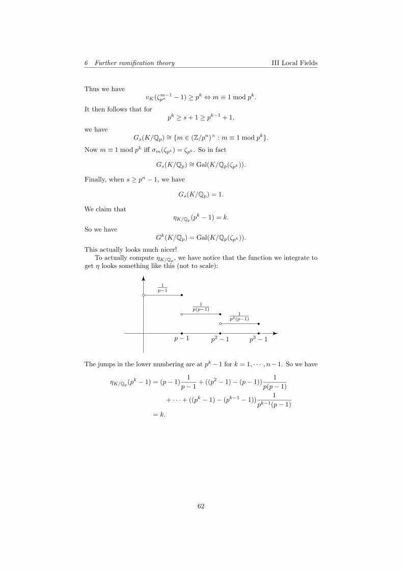
6 Further ramification theory III Local Fields
Thus we havevK(ζm−1
pn − 1) ≥ pk ⇔ m ≡ 1 mod pk.
It then follows that forpk ≥ s+ 1 ≥ pk−1 + 1,
we haveGs(K/Qp) ∼= {m ∈ (Z/pn)× : m ≡ 1 mod pk}.
Now m ≡ 1 mod pk iff σm(ζpk) = ζpk . So in fact
Gs(K/Qp) ∼= Gal(K/Qp(ζpk)).
Finally, when s ≥ pn − 1, we have
Gs(K/Qp) = 1.
We claim thatηK/Qp(pk − 1) = k.
So we haveGk(K/Qp) = Gal(K/Qp(ζpk)).
This actually looks much nicer!To actually compute ηK/Qp , we have notice that the function we integrate to
get η looks something like this (not to scale):
1p−1
1p(p−1)
1p2(p−1)
p− 1 p2 − 1 p3 − 1
The jumps in the lower numbering are at pk− 1 for k = 1, · · · , n− 1. So we have
ηK/Qp(pk − 1) = (p− 1)1
p− 1+ ((p2 − 1)− (p− 1))
1
p(p− 1)
+ · · ·+ ((pk − 1)− (pk−1 − 1))1
pk−1(p− 1)
= k.
62
7 Local class field theory III Local Fields
7 Local class field theory
Local class field theory is the study of abelian extensions of local fields, i.e. aGalois extension whose Galois group is abelian.
7.1 Infinite Galois theory
It turns out that the best way of formulating this theory is to not only use finiteextensions, but infinite extensions as well. So we need to begin with some infiniteGalois theory. We will mostly just state the relevant results instead of provingthem, because this is not a course on Galois theory.
In this section, we will work with any field.
Definition (Separable and normal extensions). Let L/K be an algebraic exten-sion of fields. We say that L/K is separable if, for every α ∈ L, the minimalpolynomial fα ∈ K[α] is separable. We say L/K is normal if fα splits in L forevery α ∈ L.
Definition (Galois extension). Let L/K be an algebraic extension of fields.Then it is Galois if it is normal and separable. If so, we write
Gal(L/K) = AutK(L).
These are all the same definitions as in the finite case.In finite Galois theory, the subgroups of Gal(L/K) match up with the
intermediate extensions, but this is no longer true in the infinite case. TheGalois group has too many subgroups. To fix this, we need to give Gal(L/K) atopology, and talk about closed subgroups.
Definition (Krull topology). Let M/K be a Galois extension. We define theKrull topology on M/K by the basis
{Gal(M/L) : L/K is finite}.
More explicitly, we say that U ⊆ Gal(M/K) is open if for every σ ∈ U , we canfind a finite subextension L/K of M/K such that σGal(M/L) ⊆ U .
Note that any open subgroup of a topological group is automatically closed,but the converse does not hold.
Note that when M/K is finite, then the Krull topology is discrete, since wecan just take the finite subextension to be M itself.
Proposition. Let M/K be a Galois extension. Then Gal(M/K) is compactand Hausdorff, and if U ⊆ Gal(M/K) is an open subset such that 1 ∈ U , thenthere is an open normal subgroup N ⊆ Gal(M/K) such that N ⊆ U .
Groups with properties in this proposition are known as profinite groups.
Proof. We will not prove the first part.For the last part, note that by definition, there is a finite subextension of
M/K such that Gal(M/L) ⊆ U . We then let L′ be the Galois closure of L overK. Then Gal(M/L′) ⊆ Gal(M/L) ⊆ U , and Gal(M/L′) is open and normal.
63
7 Local class field theory III Local Fields
Recall that we previously defined the inverse limit of a sequence rings. Moregenerally, we can define such an inverse limit for any sufficiently nice posetof things. Here we are going to do it for topological groups (for those doingCategory Theory, this is the filtered limit of topological groups).
Definition (Directed system). Let I be a set with a partial order. We say thatI is a directed system if for all i, j ∈ I, there is some k ∈ I such that i ≤ k andj ≤ k.
Example. Any total order is a directed system.
Example. N with divisibility | as the partial order is a directed system.
Definition (Inverse limit). Let I be a directed system. An inverse system (oftopological groups) indexed by I is a collection of topological groups Gi for eachi ∈ I and continuous homomorphisms
fij : Gj → Gi
for all i, j ∈ I such that i ≤ j, such that
fii = idGi
andfik = fij ◦ fjk
whenever i ≤ j ≤ k.We define the inverse limit on the system (Gi, fij) to be
lim←−i∈I
Gi =
{(gi) ∈
∏i∈I
Gi : fij(gj) = gi for all i ≤ j
}⊆∏i∈I
gi,
which is a group under coordinate-wise multiplication and a topological spaceunder the subspace topology of the product topology on
∏i∈I Gi. This makes
lim←−i∈I Gi into a topological group.
Proposition. Let M/K be a Galois extension. The set I of finite Galoissubextensions L/K is a directed system under inclusion. If L,L′ ∈ I and L ⊆ L′,then we have a restriction map
· |L′
L : Gal(L′/K)→ Gal(L/K).
Then (Gal(L/K), · |L′L ) is an inverse system, and the map
Gal(M/K)→ lim←−i∈I
Gal(L/K)
σ 7→ (σ|L)i∈I
is an isomorphism of topological groups.
We now state the main theorem of Galois theory.
64
7 Local class field theory III Local Fields
Theorem (Fundamental theorem of Galois theory). Let M/K be a Galois ex-tension. Then the map L 7→ Gal(M/L) defines a bijection between subextensionsL/K of M/K and closed subgroups of Gal(M/K), with inverse given by sendingH 7→MH , the fixed field of H.
Moreover, L/K is finite if and only if Gal(M/L) is open, and L/K is Galoisiff Gal(M/L) is normal, and then
Gal(L/K)
Gal(M/L)→ Gal(L/K)
is an isomorphism of topological groups.
Proof. This follows easily from the fundamental theorem for finite field extensions.We will only show that Gal(M/L) is closed and leave the rest as an exercise. Wecan write
L =⋃L′⊆L
L′/K finite
L′.
Then we haveGal(M/L) =
⋂L′⊆L
L′/K finite
Gal(M/L′),
and each Gal(M/L′) is open, hence closed. So the whole thing is closed.
7.2 Unramified extensions and Weil group
We first define what it means for an infinite extension to be unramified or totallyramified. To do so, we unexcitingly patch up the definitions for finite cases.
Definition (Unramified extension). Let K be a local field, and M/K be alge-braic. Then M/K is unramified if L/K is unramified for every finite subextensionL/K of M/K.
Note that since the extension is not necessarily finite, in general M will notbe a local field, since chances are its residue field would be infinite.
Definition (Totally ramified extension). Let K be a local field, and M/K bealgebraic. Then M/K is totally ramified if L/K is totally ramified for everyfinite subextension L/K of M/K.
Proposition. Let M/K be an unramified extension of local fields. Then M/Kis Galois, and
Gal(M/K) ∼= Gal(kM/kK)
via the reduction map.
Proof. Every finite subextension of M/K is unramified, so in particular is Galois.So M/K is Galois (because normality and separability is checked for eachelement). Then we have a commutative diagram
Gal(M/K) Gal(kM/kK)
lim←−L/K
Gal(L/K) lim←−L/K
Gal(kL/kK)
reduction
∼ ∼
reduction∼
65
7 Local class field theory III Local Fields
The left hand map is an isomorphism by (infinite) Galois theory, and since allfinite subextensions of kM/kK are of the form kL/kK by our finite theory, weknow the right-hand map is an isomorphism. The bottom map is an isomorphismsince it is an isomorphism in each component. So the top map must be anisomorphism.
Since the compositor of unramified extensions is unramified, it follows thatany algebraic extension M/K has a maximal unramified subextension
T = TM/K/K.
In particular, every field K has a maximal unramified extension Kur.We now try to understand unramified extensions. For a finite unramified
extension L/K, we have an isomorphism
Gal(L/K) Gal(kL/kK)∼ ,
By general field theory, we know that Gal(kL/kK) is a cyclic group generated by
FrobL/K : x 7→ xq,
where q = |kK | is the size of kK . So by the isomorphism, we obtain a generatorof Gal(L/K).
Definition (Arithmetic Frobenius). Let L/K be a finite unramified extensionof local fields, the (arithmetic) Frobenius of L/K is the lift of FrobL/K ∈Gal(kL/kK) under the isomorphism Gal(L/K) ∼= Gal(kL/kK).
There is also a geometric Frobenius, which is its inverse, but we will not usethat in this course.
We know Frob is compatible in towers, i.e. if M/L/K is a tower of finiteunramified extension of local fields, then FrobM/K |L = FrobL/K , since they both
reduce to the map x 7→ x|kK | in Gal(kL/kK), and the map between Gal(kL/kK)and Gal(L/K) is a bijection.
So if M/K is an arbitrary unramified extension, then we have an element
(FrobL/K) ∈ lim←−L/K
Gal(L/K) ∼= Gal(M/K).
So we get an element FrobM/K ∈ Gal(M/K). By tracing through the proof of
Gal(M/K) ∼= Gal(kM/kK), we see that this is the unique lift of x 7→ x|kK |.Note that while for finite unramified extensions M/K, the Galois group is
generated by the Frobenius, this is not necessarily the case when the extension isinfinite. However, powers of the Frobenius are the only things we want to thinkabout, so we make the following definition:
Definition (Weil group). Let K be a local field and M/K be Galois. LetT = TM/K be the maximal unramified subextension of M/K. The Weil groupof M/K is
W (M/K) = {σ ∈ Gal(M/K) : σ|T = FrobnT/K for some n ∈ Z}.
We define a topology on W (M/K) by saying that U is open iff there is a finiteextension L/T such that σGal(L/T ) ⊆ U .
66
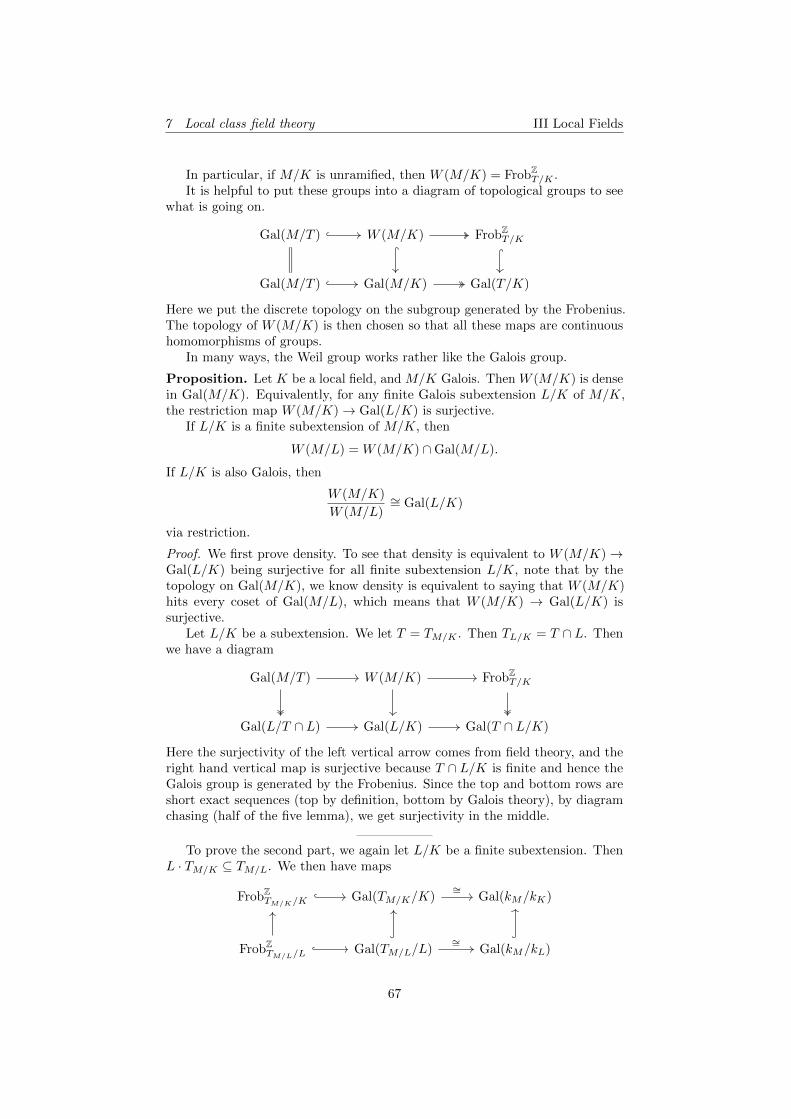
7 Local class field theory III Local Fields
In particular, if M/K is unramified, then W (M/K) = FrobZT/K .
It is helpful to put these groups into a diagram of topological groups to seewhat is going on.
Gal(M/T ) W (M/K) FrobZT/K
Gal(M/T ) Gal(M/K) Gal(T/K)
Here we put the discrete topology on the subgroup generated by the Frobenius.The topology of W (M/K) is then chosen so that all these maps are continuoushomomorphisms of groups.
In many ways, the Weil group works rather like the Galois group.
Proposition. Let K be a local field, and M/K Galois. Then W (M/K) is densein Gal(M/K). Equivalently, for any finite Galois subextension L/K of M/K,the restriction map W (M/K)→ Gal(L/K) is surjective.
If L/K is a finite subextension of M/K, then
W (M/L) = W (M/K) ∩Gal(M/L).
If L/K is also Galois, then
W (M/K)
W (M/L)∼= Gal(L/K)
via restriction.
Proof. We first prove density. To see that density is equivalent to W (M/K)→Gal(L/K) being surjective for all finite subextension L/K, note that by thetopology on Gal(M/K), we know density is equivalent to saying that W (M/K)hits every coset of Gal(M/L), which means that W (M/K) → Gal(L/K) issurjective.
Let L/K be a subextension. We let T = TM/K . Then TL/K = T ∩ L. Thenwe have a diagram
Gal(M/T ) W (M/K) FrobZT/K
Gal(L/T ∩ L) Gal(L/K) Gal(T ∩ L/K)
Here the surjectivity of the left vertical arrow comes from field theory, and theright hand vertical map is surjective because T ∩ L/K is finite and hence theGalois group is generated by the Frobenius. Since the top and bottom rows areshort exact sequences (top by definition, bottom by Galois theory), by diagramchasing (half of the five lemma), we get surjectivity in the middle.
To prove the second part, we again let L/K be a finite subextension. ThenL · TM/K ⊆ TM/L. We then have maps
FrobZTM/K/K
Gal(TM/K/K) Gal(kM/kK)
FrobZTM/L/L
Gal(TM/L/L) Gal(kM/kL)
∼=
∼=
67
7 Local class field theory III Local Fields
So the left hand vertical map is an inclusion. So we know
FrobZTM/L/L
= FrobZTM/K/K
∩Gal(TM/L/L).
Now if σ ∈ Gal(M/L), then we have
σ ∈W (M/L)⇔ σ|TM/L/L ∈ FrobZTM/L/L
⇔ σ|TM/K/K ∈ FrobZTM/K/K
⇔ σ ∈W (M/K).
So this gives the second part.
Now L/K is Galois as well. Then Gal(M/L) is normal in Gal(M/K). SoW (M/L) is normal in W (M/K) by the second part. Then we can compute
W (M/K)
W (M/L)=
W (M/K)
W (M/K) ∩Gal(M/L)
∼=W (M/K) Gal(M/L)
Gal(M/L)
=Gal(M/K)
Gal(M/L)∼= Gal(L/K).
The only non-trivial part in this chain is the assertion thatW (M/K) Gal(M/L) =Gal(M/K), i.e. that W (M/K) hits every coset of Gal(M/L), which is whatdensity tells us.
7.3 Main theorems of local class field theory
We now come to the main theorems of local class field theory.
Definition (Abelian extension). Let K be a local field. A Galois extensionL/K is abelian if Gal(L/K) is abelian.
We will fix an algebraic closure K of K, and all algebraic extensions we willconsider will be taken to be subextensions of K/K. We let Ksep be the separableclosure of K inside K.
If M/K and M/K are Galois extensions, then LM/K is Galois, and the mapgiven by restriction
Gal(LM/K) ↪→ Gal(L/K)×Gal(M/K).
is an injection. In particular, if L/K and M/K are both abelian, then so isLM/K. This implies that there is a maximal abelian extension Kab.
Finally, note that we know an example of an abelian extension, namely themaximal unramified extension Kur = TKsep/K ⊆ Kab, and we put FrobK =FrobKur/K .
Theorem (Local Artin reciprocity). There exists a unique topological isomor-phism
ArtK : K× →W (Kab/K)
characterized by the properties
68
7 Local class field theory III Local Fields
(i) ArtK(πK)|Kur = FrobK , where πK is any uniformizer.
(ii) We haveArtK(NL/K(x))|L = idL
for all L/K finite abelian and x ∈ L×.
Moreover, if M/K is finite, then for all x ∈ M×, we know ArtM (x) is anautomorphism of Mab/M , and restricts to an automorphisms of Kab/K. Thenwe have
ArtM (x)|Kab
K = ArtK(NM/K(x)).
Moreover, ArtK induces an isomorphism
K×
NM/K(M×)→ Gal
(M ∩Kab
K
).
To simplify this, we will write N(L/K) = NL/K(L×) for L/K finite. Fromthis theorem, we can deduce a lot of more precise statements.
Corollary. Let L/K be finite. Then N(L/K) = N((L ∩Kab)/K), and
(K× : N(L/K)) ≤ [L : K]
with equality iff L/K is abelian.
Proof. To see this, we let M = L ∩Kab. Applying the isomorphism twice gives
K×
N(L/K)∼= Gal(M/K) ∼=
K×
N(M/K).
Since N(L/K) ⊆ N(M/K), and [L : K] ≥ [M : K] = |Gal(M/K)|, we aredone.
The theorem tells us if we have a finite abelian extension M/K, then weobtain an open finite-index subgroup NM/K(M×) ≤ K×. Conversely, if we aregiven an open finite index subgroup of K×, we might ask if there is an abelianextension of K whose norm group is corresponds to this subgroup. The followingtheorem tells us this is the case:
Theorem. Let K be a local field. Then there is an isomorphism of posets{open finite indexsubgroups of K×
} {finite abelian
extensions of L/K
}H (Kab)ArtK(H)
N(L/K) L/K
.
In particular, for L/K and M/K finite abelian extensions, we have
N(LM/K) = N(L/K) ∩N(M/K),
N(L ∩M/K) = N(L/K)N(M/K).
69
7 Local class field theory III Local Fields
While proving this requires quite a bit of work, a small part of it follows fromlocal Artin reciprocity:
Theorem. Let L/K be a finite extension, and M/K abelian. Then N(L/K) ⊆N(M/K) iff M ⊆ L.
Proof. By the previous theorem, we may wlog L/K abelian by replacing withL ∩Kab. The ⇐ direction is clear by the last part of Artin reciprocity.
For the other direction, we assume that we have N(L/K) ⊆ N(M/K), andlet σ ∈ Gal(Kab/L). We want to show that σ|M = idM . This would then implythat M is a subfield of L by Galois theory.
We know W (Kab/L) is dense in Gal(Kab/L). So it suffices to show this forσ ∈W (Kab/L). Then we have
W (Kab/L) ∼= ArtK(N(L/K)) ⊆ ArtK(N(M/K)).
So we can find x ∈M× such that σ = ArtK(NM/K(x)). So σ|M = idM by localArtin reciprocity.
Side note: Why is this called “class field theory”? Usually, we call the fieldcorresponding to the subgroup H the class field of H. Historically, the first typeof theorems like this are proved for number fields. The groups that appear onthe left would be different, but in some cases, they are the class group of thenumber field.
70
8 Lubin–Tate theory III Local Fields
8 Lubin–Tate theory
For the rest of the course, we will indicate how one can explicitly construct thefield Kab and the map ArtK .
There are many ways we can approach local class field theory. The approachwe use, using Lubin–Tate theory, is the most accessible one. Another possibleapproach is via Galois cohomology. This, however, relies on more advancedmachinery, namely Galois cohomology.
8.1 Motivating example
We will work out the details of local Artin reciprocity in the case of Qp as amotivating example for the proof we are going to come up with later. Here wewill need the results of local class field theory to justify our claims, but this isnot circular since this is not really part of the proof.
Lemma. Let L/K be a finite abelian extension. Then we have
eL/K = (O×K : NL/K(O×L )).
Proof. Pick x ∈ L×, and w the valuation on L extending vK , and n = [L : K].Then by construction of w, we know
vK(NL/K(x)) = nw(x) = fL/KvL(x).
So we have a surjection
K×
N(L/K)
ZfL/KZ
vK .
The kernel of this map is equal to
O×KN(L/K)
N(L/K)∼=
O×KO×K ∩N(L/K)
=O×K
NL/K(O×L ).
So by local class field theory, we know
n = (K× : N(L/K)) = fL/K(O×K : NL/K(O×L )),
and this implies what we want.
Corollary. Let L/K be a finite abelian extension. Then L/K is unramified ifand only if NL/K(O×L ) = O×K .
Now we fix a uniformizer πK . Then we have a topological group isomorphism
K× ∼= 〈πK〉 × O×K .
Since we know that the finite abelian extensions correspond exactly to finiteindex subgroups of K× by taking the norm groups, we want to understandsubgroups of K×. Now consider the subgroups of K× of the form
〈πmK 〉 × U(n)K .
71
8 Lubin–Tate theory III Local Fields
We know these form a basis of the topology of K×, so it follows that finite-indexopen subgroups must contain one of these guys. So we can find the maximalabelian extension as the union of all fields corresponding to these guys.
Since we know that N(LM/K) = N(L/K) ∩N(M/K), it suffices to furtherspecialize to the cases
〈πK〉 × U (n)K
and〈πmK 〉 × OK
separately. The second case is easy, because this corresponds to an unramifiedextension by the above corollary, and unramified extensions are completelycharacterized by the extension of the residue field. Note that the norm group andthe extension are both independent of the choice of uniformizer. The extensionscorresponding to the first case are much more difficult to construct, and theydepend on the choice of πK . We will get them from Lubin–Tate theory.
Lemma. Let K be a local field, and let Lm/K be the extension correspondingto 〈πmK 〉 × OK . Let
L =⋃m
Lm.
Then we haveKab = KurL,
Lemma. We have isomorphisms
W (Kab/K) ∼= W (KurL/K)∼= W (Kur/K)×Gal(L/K)
∼= FrobZK ×Gal(L/K)
Proof. The first isomorphism follows from the previous lemma. The secondfollows from the fact that Kur ∩ L = K as L is totally ramified. The lastisomorphism follows from the fact that TKur/K = Kur trivially, and then by
definition W (Kur/K) ∼= FrobZK .
Example. We consider the special case of K = Qp and πK = p. We let
Ln = Qp(ζpn),
where ζpn is the primitive pnth root of unity. Then by question 6 on examplesheet 2, we know this is a field with norm group
N(Qp(ζpn)/Qp) = 〈p〉 × (1 + pnZp) = 〈p〉 × U (n)Qp ,
and thus this is a totally ramified extension of Qp.We put
Qp(ζp∞) =
∞⋃n=1
Qp(ζpn).
Then again this is totally ramified extension, since it is the nested union oftotally ramified extensions.
72
8 Lubin–Tate theory III Local Fields
Then we have
Gal(Qp(ζp∞)/Qp) ∼= lim←−n
Gal(Qp(ζpn)/Qp)
= lim←−n
(Z/pnZ)×
= Z×p .
Note that we are a bit sloppy in this deduction. While we know that it is truethat Z×p ∼= lim←−n(Z/pnZ)×, the inverse limit depends not only on the groups
(Z/pnZ)× themselves, but also on the maps we use to connect the groups together.Fortunately, from the discussion below, we will see that the maps
Gal(Qp(ζpn)/Qp)→ Gal(Qp(ζpn−1)/Qp)
indeed correspond to the usual restriction maps
(Z/pnZ)× → (Z/pn−1Z)×.
It is a fact that this is the inverse of the Artin map of Qp restricted to Z×p .Note that we have W (Qp(ζp∞)/Qp) = Gal(Qp(ζp∞)/Qp) because its maximalunramified subextension is trivial.
We can trace through the above chains of isomorphisms to figure out whatthe Artin map does. Let m = Z×p . Then we can write
m = a0 + a1p+ · · · ,
where ai ∈ {0, · · · , p− 1} and a0 6= 0. Now for each n, we know
m ≡ a0 + a1p+ · · ·+ an−1pn−1 mod pn.
By the usual isomorphism Gal(Qp(ζpn)/Qp) ∼= Z/pnZ, we know m acts as
ζpn 7→ ζa0+a1p+...+an−1p
n−1
pn “=” ζmpn
on Qp(ζpn), where we abuse notation because taking ζpn to powers of p greaterthan n gives 1. It can also be interpreted as (1 + λpn)m, where λpn = ζpn − 1 isa uniformizer, which makes sense using binomial expansion.
So the above isomorphisms tells us that ArtQp restricted to Z×p acts onQp(ζp∞) as
ArtQp(m)(ζpn) ≡ σm−1(ζpn) = ζm−1
pn .
The full Artin map can then be read off from the following diagram:
Q×p W (Qabp /Qp)
〈p〉 × Z×p W (Qurp /Qp)×Gal(Qp(ζp∞)/Qp)
∼=
ArtQp
restriction∼
where the bottom map sends
〈pn,m〉 7→ (FrobnQp , σm−1).
73
8 Lubin–Tate theory III Local Fields
In fact, we have
Theorem (Local Kronecker-Weber theorem).
Qabp =
⋃n∈Z≥1
Qp(ζn),
Qurp =
⋃n∈Z≥1
(n,p)=1
Qp(ζn).
Not a proof. We will comment on the proof of the generalized version later.
Remark. There is another normalization of the Artin map which sends auniformizer to the geometric Frobenius , defined to be the inverse of the arithmeticFrobenius. With this convention, ArtQp(m)|Qp(ζp∞ ) is σm.
We can define higher ramification groups for general Galois extensions.
Definition (Higher ramification groups). Let K be a local field and L/K Galois.We define, for s ∈ R≥−1
Gs(M/K) = {σ ∈ Gal(M/K) : σ|L ∈ Gs(L/K) for all finite
Galois subextension M/K}.
This definition makes sense, because the upper number behaves well whenwe take quotients. This is one of the advantages of upper numbering. Note thatwe can write the ramification group as the inverse limit
Gs(M/K) ∼= lim←−L/K
Gs(L/K),
as in the case of the Galois group.
Example. Going back to the case of K = Qp. We write Qpn for the unramifiedextension of degree n of Qp. By question 11 of example sheet 3, we know that
Gs(Qpn(ζpm)/Qp) =
Gal(Qpn(ζpm)/Qp) s = −1
Gal(Qpn(ζpm)/Qpn) −1 < s ≤ 0
Gal(Qpn(ζpm)/ζpk) k − 1 < s ≤ k ≤ m− 1
1 s > m− 1
,
which corresponds to
〈p〉 × U (0)
〈pn〉 × U (m)s = −1
〈pn〉 × U (0)
〈pn〉 × U (m)−1 < s ≤ 0
〈pn〉 × U (k)
〈pn〉 × U (m)k − 1 < s ≤ k ≤ m− 1
1 s > m− 1
under the Artin map.
74
8 Lubin–Tate theory III Local Fields
By taking the limit as n,m→∞, we get
Theorem. We have
Gs(Qabp /Qp) = ArtQp(1 + pkZp) = ArtQp(U (k)),
where k is chosen such that k − 1 < s ≤ k, k ∈ Z≥0.
Corollary. If L/Qp is a finite abelian extension, then
Gs(L/Qp) = ArtQp
(N(L/Qp)(1 + pnZp)
N(L/Qp)
),
where n− 1 < s ≤ n.
Here ArtQp induces an isomorphism
Q×pN(L/Qp)
→ Gal(L/Qp).
So it follows that L ⊆ Qp(ζpm) for some n if and only if Gs(L/Qp) = 1 for alls > m− 1.
8.2 Formal groups
The proof of local Artin reciprocity will be done by constructing the analogousversions of Ln for an arbitrary local field, and then proving that it works. Todo so, we will need the notion of a formal group. The idea of a formal group isthat a formal group is a rule that specifies how we should multiply two elementsvia a power series over a ring R. Then if we have a complete R-module, thenthe formal group will turn the R-module into an actual group. There is then anatural notion of a formal module, which is a formal group F with an R-action.
At the end, we will pick R = OK . The idea is then that we can fix analgebraic closure K, and then a formal OK -module will turn mK into an actualOK-module. Then if we adjoin the right elements of mK to K, then we obtainan extension of K with a natural OK action, and we can hope that this restrictsto field automorphisms when we restrict to the unit group.
Notation. Let R be a ring. We write
R[[x1, · · · , xn]] =
∑k1,...,kn∈Z≥0
ak1,...,knxk11 · · ·xknn : ak1,...,kn ∈ R
for the ring of formal power series in n variables over R.
Definition (Formal group). A (one-dimensional, commutative) formal groupover R is a power series F (X,Y ) ∈ R[X,Y ] such that
(i) F (X,Y ) ≡ X + Y mod (X2, XY, Y 2)
(ii) Commutativity: F (X,Y ) = F (Y,X)
(iii) Associativity: F (X,F (Y,Z)) = F (F (X,Y ), Z).
75
8 Lubin–Tate theory III Local Fields
This is most naturally understood from the point of view of algebraic geometry,as a generalization of the Lie algebra over a Lie group. Instead of talking aboutthe tangent space of a group (the “first-order neighbourhood”), we talk about itsinfinitesimal (formal) neighbourhood, which contains all higher-order information.A lot of the seemingly-arbitrary compatibility conditions we later impose havesuch geometric motivation that we unfortunately cannot go into.
Example. If F is a formal group over OK , where K is a complete valued field,then F (x, y) converges for all x, y ∈ mK . So mK becomes a (semi)group underthe multiplication
(x, y) 7→ F (x, y) ∈ mk
Example. We can define
Ga(X,Y ) = X + Y.
This is called the formal additive group.Similarly, we can have
Gm(X,Y ) = X + Y +XY.
This is called the formal multiplicative group. Note that
X + Y +XY = (1 +X)(1 + Y )− 1.
So if K is a complete valued field, then mK bijects with 1 + mk by sendingx 7→ 1 + x, and the rule sending (x, y) ∈ m2
K 7→ x + y + xy ∈ mK is just theusual multiplication in 1 + mK transported to mK via the bijection above.
We can think of this as looking at the group in a neighbourhood of theidentity 1.
Note that we called this a formal group, rather than a formal semi-group. Itturns out that the existence of identity and inverses is automatic.
Lemma. Let R be a ring and F a formal group over R. Then
F (X, 0) = X.
Also, there exists a power series i(X) ∈ X ·R[[X]] such that
F (X, i(X)) = 0.
Proof. See example sheet 4.
The next thing to do is to define homomorphisms of formal groups.
Definition (Homomorphism of formal groups). Let R be a ring, and F,G beformal groups over R. A homomorphism f : F → G is an element f ∈ R[[X]]such that f(X) ≡ 0 mod X and
f(F (X,Y )) = G(f(X), f(Y )).
The endomorphisms f : F → F form a ring EndR(F ) with addition +F given by
(f +F g)(x) = F (f(x), g(x)).
and multiplication is given by composition.
76
8 Lubin–Tate theory III Local Fields
We can now define a formal module in the usual way, plus some compatibilityconditions.
Definition (Formal module). Let R be a ring. A formal R-module is a formalgroup F over R with a ring homomorphism R→ EndR(F ), written, a 7→ [a]F ,such that
[a]F (X) = aX mod X2.
Those were all general definitions. We now restrict to the case we really careabout. Let K be a local field, and q = |kK |. We let π ∈ OK be a uniformizer.
Definition (Lubin–Tate module). A Lubin–Tate module over OK with respectto π is a formal OK-module F such that
[π]F (X) ≡ Xq mod π.
We can think of this condition of saying “uniformizer corresponds to theFrobenius”.
Example. The formal group Gm is a Lubin–Tate Zp module with respect to pgiven by the following formula: if a ∈ Zp, then we define
[a]Gm(X) = (1 +X)a − 1 =
∞∑n=1
(a
n
)Xn.
The conditions(1 +X)a − 1 ≡ aX mod X2
and(1 +X)p − 1 ≡ Xp mod p
are clear.We also have to check that a 7→ [a]F is a ring homomorphism. This follows
from the identities
((1 +X)a)b = (1 +X)ab, (1 +X)a(1 +X)b = (1 +X)ab,
which are on the second example sheet.
The objective of the remainder of the section is to show that all Lubin–Tatemodules are isomorphic.
Definition (Lubin–Tate series). A Lubin–Tate series for π is a power seriese(X) ∈ OK [[X]] such that
e(X) ≡ πX mod X2, e(X) ≡ Xq mod π.
We denote the set of Lubin–Tate series for π by Eπ.
Now by definition, if F is a Lubin–Tate OK module for π, then [π]F is aLubin–Tate series for π.
Definition (Lubin–Tate polynomial). A Lubin–Tate polynomial is a polynomialof the form
uXq + π(aq−1Xq−1 + · · ·+ a2X
2) + πX
with u ∈ U (1)K , and aq−1, · · · , a2 ∈ OK .
In particular, these are Lubin–Tate series.
77
8 Lubin–Tate theory III Local Fields
Example. Xq + πX is a Lubin–Tate polynomial.
Example. If K = Qp and π = p, then (1 +X)p− 1 is a Lubin–Tate polynomial.
The result that allows us to prove that all Lubin–Tate modules are isomorphicis the following general result:
Lemma. Let e1, e2 ∈ Eπ and take a linear form
L(x1, · · · , xn) =
n∑i=1
aiXi, ai ∈ OK .
Then there is a unique power series F (x1, · · · , xn) ∈ OK [[x1, · · · , xn]] such that
F (x1, · · · , xn) ≡ L(x1, · · · , xn) mod (x1, · · · , xn)2,
ande1(F (x1, · · · , xn)) = F (e2(x1), e2(x2), · · · , e2(xn)).
For reasons of time, we will not prove this. We just build F by successiveapproximation, which is not terribly enlightening.
Corollary. Let e ∈ Eπ be a Lubin–Tate series. Then there are unique powerseries Fe(X,Y ) ∈ OK [[X,Y ]] such that
Fe(X,Y ) ≡ X + Y mod (X + Y )2
e(Fe(X,Y )) = Fe(e(X), E(Y ))
Corollary. Let e1, e2 ∈ Eπ be Lubin–Tate series and a ∈ OK . Then there existsa unique power series [a]e1,e2 ∈ OK [[X]] such that
[a]e1,e2(X) ≡ aX mod X2
e1([a]e1,e2(X)) = [a]e1,e2(e2(X)).
To simplify notation, if e1 = e2 = e, we just write [a]e = [a]e,e.
We now state the theorem that classifies all Lubin–Tate modules in terms ofLubin–Tate series.
Theorem. The Lubin–Tate OK modules for π are precisely the series Fe fore ∈ Eπ with formal OK-module structure given by
a 7→ [a]e.
Moreover, if e1, e2 ∈ Eπ and a ∈ OK , then [a]e1,e2 is a homomorphism fromFe2 → Fe1 .
If a ∈ O×K , then it is an isomorphism with inverse [a−1]e2,e1 .
So in some sense, there is only one Lubin–Tate module.
Proof sketch. If F is a Lubin–Tate OK-module for π, then e = [π]F ∈ Eπ bydefinition, and F satisfies the properties that characterize the series Fe. SoF = Fe by uniqueness.
For the remaining parts, one has to verify the following for all e, e1, e2, e3 ∈ Eπand a, b ∈ OK .
78
8 Lubin–Tate theory III Local Fields
(i) Fe(X,Y ) = Fe(Y,X).
(ii) Fe(X,Fe(Y,Z)) = Fe(Fe(X,Y ), Z).
(iii) [a]e1,e2(Fe(X,Y )) = Fe1([a]e1,e2(X), [a]e1,e2(Y )).
(iv) [ab]e1,e3(X) = [a]e1,e2([b]e2,e3(X)).
(v) [a+ b]e1,e2(X) = [a]e1,e2(X) + [b]e1,e2(X).
(vi) [π]e(X) = e(X).
The proof is just repeating the word “uniqueness” ten times.
8.3 Lubin–Tate extensions
We now use the Lubin–Tate modules to do things. As before, we fixed analgebraic closure K of K. We let m = mK be the maximal ideal in OK .
Proposition. If F is a formal OK-module, then m becomes a (genuine) OKmodule under the operations +F and ·
x+F y = F (x, y)
a · x = [a]F (x)
for all x, y ∈ m and a ∈ OK .We denote this mF .
This isn’t exactly immediate, because K need not be complete. However,this is not a problem as each multiplication given by F only involves finitelymany things (namely two of them).
Proof. If x, y ∈ m, then F (x, y) is a series in K(x, y) ⊆ K. Since K(x, y) isa finite extension, we know it is complete. Since the terms in the sum haveabsolute value < 1 and → 0, we know it converges to an element in mK(x,y) ⊆ m.The rest then essentially follows from definition.
To prove local class field theory, we want to find elements with an UK/U(n)K
action for each n, or equivalently elements with an OK/O(n)K action. Note that
the first quotient is a quotient of groups, while the second quotient is a quotientof a ring by an ideal. So it is natural to consider the following elements:
Definition (πn-division points). Let F be a Lubin–Tate OK -module for π. Letn ≥ 1. The group F (n) of πn-division points of F is defined to be
F (n) = {x ∈ mF | [πn]Fx = 0} = ker([πn]F ).
This is a group under the operation given by F , and is indeed an OK module.
Example. Let F = Gm,K = Qp and π = p. Then for x ∈ mGm , we have
pn · x = (1 + x)pn
− 1.
So we knowGm(n) = {ζipn − 1 | i = 0, 1, · · · , pn − 1},
where ζpn ∈ Qp is the primitive pnth root of unity.
So Gm(n) generates Qp(ζpn).
79
8 Lubin–Tate theory III Local Fields
To prove this does what we want, we need the following lemma:
Lemma. Let e(X) = Xq + πX. We let
fn(X) = (e ◦ · · · ◦ e)︸ ︷︷ ︸n times
(X).
Then fn has no repeated roots. Here we take f0 to be the identity function.
Proof. Let x ∈ K. We claim that if |fi(x)| < 1 for i = 0, · · · , n − 1, thenf ′n(X) 6= 0.
We proceed by induction on n.
(i) When n = 1, we assume |x| < 1. Then
f ′1(x) = e′(x) = qxq−1 + π = π(
1 +q
πxq−1
)6= 0,
since we know qπ has absolute value ≤ 1 (q vanishes in kK , so q/π lives in
OK), and xq−1 has absolute value < 1.
(ii) in the induction step, we have
f ′n+1(x) = (qfn(x)q−1 + π)f ′n(x) = π(
1 +q
πfn(x)q−1
)f ′n(x).
By induction hypothesis, we know f ′n(x) 6= 0, and by assumption |fn(x)| <1. So the same argument works.
We now prove the lemma. We assume that fn(x) = 0. We want to show that|fi(x)| < 1 for all i = 0, · · · , n− 1. By induction, we have
fn(x) = xqn
+ πgn(x)
for some gn(x) ∈ OK [x]. It follows that if fn(x) = 0, then |x| < 1. So |fi(x)| < 1for all i. So f ′n(x) 6= 0.
The point of the lemma is to prove the following proposition:
Proposition. F (n) is a free OK/πnOK module of rank 1. In particular, it hasqn elements.
Proof. By definition, we know
πn · F (n) = 0.
So F (n) is indeed an OK/πnOK-module.To prove that it is free of rank 1, we note that all Lubin–Tate modules
for π are isomorphic. This implies that all the honest OK modules F (n) areisomorphic. We choose F = Fe, where e = Xq + πX. Then F (n) consistsof the roots of the polynomial fn = en(X), which is of degree qn and has norepeated roots. So |F (n)| = qn. To show that it is actually the right thing, ifλn ∈ F (n) \ F (n− 1), then we have a homomorphism
OK → F (n)
80
8 Lubin–Tate theory III Local Fields
given by A 7→ a · λn. Its kernel is πnOK by our choice of λn. By counting, weget an OK-module isomorphism
OKπnOK
→ F (n)
as desired.
Corollary. We have isomorphisms
OKπnOK
∼= EndOK (F (n))
UK
U(n)K
∼= AutOK (F (n)).
Given a Lubin–Tate OK-module F for π, we consider
Ln,π = Ln = K(F (n)),
which is the field of πn division points of F . From the inclusions F (n) ⊆ F (n+1)for all n, we obtain a corresponding inclusion of fields
Ln ⊆ Ln+1.
The field Ln depends only in π, and not on F . To see this, we let G be anotherLubin–Tate OK-module, and let f : F → G be an isomorphism. Then
G(n) = f(F (n)) ⊆ K(F (n))
since the coefficients of f lie in K. So we know
K(G(n)) ⊆ K(F (n)).
By symmetry, we must have equality.
Theorem. Ln/K is a totally ramified abelian extension of degree qn−1(q − 1)with Galois group
Gal(Ln/K) ∼= AutOK (F (n)) ∼=UK
U(n)K
.
Explicitly, for any σ ∈ Gal(Ln/K), there is a unique u ∈ UK/U (n)K such that
σ(λ) = [u]F (λ)
for all λ ∈ F (n). Under this isomorphism, for m ≥ n, we have
Gal(Lm/Ln) ∼=U
(n)K
U(m)K
.
Moreover, if F = Fe, where
e(X) = Xq + π(aq−1πq−1 + · · ·+ a2X
2) + πX,
81
8 Lubin–Tate theory III Local Fields
and λn ∈ F (n) \ F (n− 1), then λn is a uniformizer of Ln and
φn(X) =en(X)
en−1(X)= Xqn−1(q−1) + · · ·+ π
is the minimal polynomial of λn. In particular,
NLn/K(−λn) = π.
Proof. Consider a Lubin–Tate polynomial
e(X) = xq + π(aq−1Xq−1 + · · ·+ a2X
2) + πX.
We set F = Fe. Then
φn(X) =en(X)
en−1(X)= (en−1(X))q−1 + π(aq1e
n−1(X)q−2 + · · ·+ a2en−1(X)) + π
is an Eisenstein polynomial of degree qn−1(q − 1) by starting at it long enough.So if λn ∈ F (n) \ F (n − 1), then λn is a root of φn(x), so K(λn)/K is totallyramified of degree qn−1(q − 1), and λn is a uniformizer, and
NK(λn)/K(−λn) = π
as the norm is just the constant coefficient of the minimal polynomial.Now let σ ∈ Gal(Ln/K). Then σ induces a permutation of F (n), as these
are the roots of en(X), which is in fact OK-linear, i.e.
σ(x) +F σ(y) = F (σ(x), σ(y)) = σ(F (x, y)) = σ(x+F y)
σ(a · x) = σ([a]F (x)) = [a]F (σ(x)) = a · σ(x)
for all x, y ∈ mLn and a ∈ OK .So we have an injection of groups
Gal(Ln/K) ↪→ AutOK (F (n)) =UK
U(n)K
But we know∣∣∣∣∣ UKU (n)K
∣∣∣∣∣ = qn−1(q − 1) = [K(λn) : K] ≤ [Ln : K] = |Gal(Ln/K)|.
So we must have equality throughout, the above map is an isomorphism, andK(λn) = Ln.
It is clear from the construction of the isomorphism that for m ≥ n, thediagram
Gal(Lm/K) UK/U(m)K
Gal(Ln/K) UK/U(n)K
∼
restriction quotient
∼
commutes. So the isomorphism
Gal(Lm/Ln) ∼=U
(m)K
U(n)K
follows by looking at the kernels.
82
8 Lubin–Tate theory III Local Fields
Example. In the case where K = Qp and π = p, recall that
Gm(n) = {ζipn − 1 | i = 0, · · · , pn−1 − 1},
where ζpn is the principal pnth root of unity. The theorem then gives
Gal(Qp(ζpn)/Qp) ∼= (Z/pn)×
given by if a ∈ Z≥0 and (a, p) = 1, then
σa(ζipn − 1) = [a]Gm(n)(ζipn − 1) = (1 + (ζipn − 1))a − 1 = ζaipn − 1.
This agrees with the isomorphism we previously constructed.
Back to the general situation, setting
L∞ =
∞⋃n=1
Ln,
we know L∞/K is Galois, and we have isomorphisms
Gal(L∞/K) lim←−Gal(Ln/K) lim←−n UK/U(n)K∼= UK
σ (σ|Ln)n
∼ ∼
This map will be the inverse of the Artin map restricted to L∞.To complete the proof of Artin reciprocity, we need to use the following
theorem without proof:
Theorem (Generalized local Kronecker-Weber theorem). We have
Kab = KurL∞
(for any π).
Comments on the proof. One can prove this from the Hasse-Arf theorem, whichstates that in an abelian extension, the jumps in the upper ramification groupsoccur only at integer values. This, together with the calculation of ramificationgroups done later, easily implies the theorem. Essentially, L∞ maxed out allpossible jumps of the upper ramification groups. However, the Hasse-Arf theoremis difficult to prove.
Another approach is to prove the existence of the Artin map using othertechniques (e.g. Galois cohomology). Consideration of the norm group (cf. thenext theorem) then implies the theorem. The content of this section thenbecomes an explicit construction of a certain family of abelian extensions.
We can characterize the norm group by
Theorem. We haveN(Ln/K) = 〈π〉 × U (n)
k .
Comments on the proof. This can be done by defining Coleman operators , whichare power series representations of the norm. Alternatively, assuming the
description of the local Artin map given below and local Artin reciprocity, U(n)k
is in the kernel of Art|Ln , so 〈π〉 × U (n)k ⊆ N(Ln/K). The result follows by
comparing order.
83
8 Lubin–Tate theory III Local Fields
We can then construct the Artin map as follows:
Theorem. Let K be a local field. Then we have an isomorphism Art : K× →W (Kab/K) given by the composition
K× W (Kab/K)
〈π〉 × UK FrobZK ×Gal(L∞/K)
∼
Art
∼
where the bottom map is given by (πm, u) 7→ (FrobmK , σu−1), where
σu(λ) = [u]F (λ)
for all λ ∈⋃∞n=1 F (n).
The inverse shows up in the proof to make sure the map defined above isindependent of the choice of uniformizer. We will not prove this, nor that themap obtained has the desired properties. Instead, we will end the course bycomputing the higher ramification groups of these extensions.
Theorem. We have
Gs(Ln/K) =
Gal(Ln/K) −1 ≤ s ≤ 0
Gal(Ln/Lk) qk−1 − 1 < s ≤ qk − 1, 1 ≤ k ≤ n− 1
1 s > qn−1
Proof. The case for −1 ≤ s ≤ 0 is clear.For 0 ≤ s ≤ 1 (which we may wlog is actually 1), we know that
Gal(Ln/Lk) ∼= U(k)K /U
(n)K
under the isomorphism Gal(Ln/K) ∼= UK/U(n)K . On the other hand, we know
G1(Ln/K) is the Sylow p-subgroup of Gal(Ln/K). So we must have
G1(Ln/K) ∼= U(1)K /U
(n)K .
So we know that G1(Ln/K) = Gal(Ln/L1). Thus we know that Gs(Ln/K) =Gal(Ln/K) for 0 < s ≤ 1.
We now let σ = σu ∈ G1(Ln/K) and u ∈ U (1)K /U
(n)K . We write
u = 1 + επk
for some ε ∈ UK and some k = k(u) ≥ 1. Since σ is not the identity, we knowk < n. We claim that
iLn/K(σ) = vLn(σ(λ)− λ) = qk.
Indeed, we let λ ∈ F (n) \ F (n− 1), where F is a choice of Lubin–Tate modulefor π. Then λ is a uniformizer of Ln and OLn = OK [λ]. We can compute
σu(λ) = [u]F (λ)
= [1 + επk]F (λ)
= F (λ, [επk]F (λ))
84
8 Lubin–Tate theory III Local Fields
Now we can write
[επk]F (λ) = [ε]F ([πk]F (λ)) ∈ F (n− k) \ F (n− k − 1),
since [ε]F is invertible, and applying [πn−k]F to [πk]F (λ) kills it, but applying[πn−k−1]F gives [πn−1]F , which does not kill.
So we know [επk]F (λ) is a uniformizer of Ln−k. Since Ln/Ln−k is totallyramified of degree qk, we can find ε0 ∈ O×Ln such that
[επk]F (λ) = ε0λqk
Recall that F (X, 0) = X and F (0, Y ) = Y . So we can write
F (X,Y ) = X + Y +XYG(X,Y ),
where G(X,Y ) ∈ OK [[X,Y ]]. So we have
σ(λ)− λ = F (λ, [επk]F (λ))− λ
= F (λ, ε0λqk)− λ
= λ+ ε0λqk + ε0λ
qk+1G(λ, ε0λqk)− λ
= ε0λqk + ε0λ
qk+1G(λ, ε0λqk).
In terms of valuation, the first term is the dominating term, and
iLn/K(σ) = vLn(σ(λ)− λ) = qk
So we knowiLn/K(σk) ≥ s+ 1⇔ qk(u) − 1 ≥ s.
So we know
Gs(Ln/K) = {σK ∈ G1(Ln/K) : qk(u) − 1 ≥ s} = Gal(Ln/Lk),
where qk−1 − 1 < s ≤ qk − 1 for k = 1, · · · , n− 1, and 1 if s > qn−1 = 1.
Corollary. We have
Gt(Ln/K) =
Gal(Ln/K) −1 ≤ t ≤ 0
Gal(Ln/Lk) k − 1 < t ≤ k, k = 1, · · · , n− 1
1 t > n− 1
In other words, we have
Gt(Ln/K) =
{Gal(Ln/Ldte) −1 ≤ t ≤ n− 1
1 t > n− 1,
where we set L0 = K.
Once again, the numbering is a bit more civilized in the upper numbering.
Proof. We have to compute the integral of
1
(G0(Ln/K) : Gx(Ln/K).
We again plot this out
85
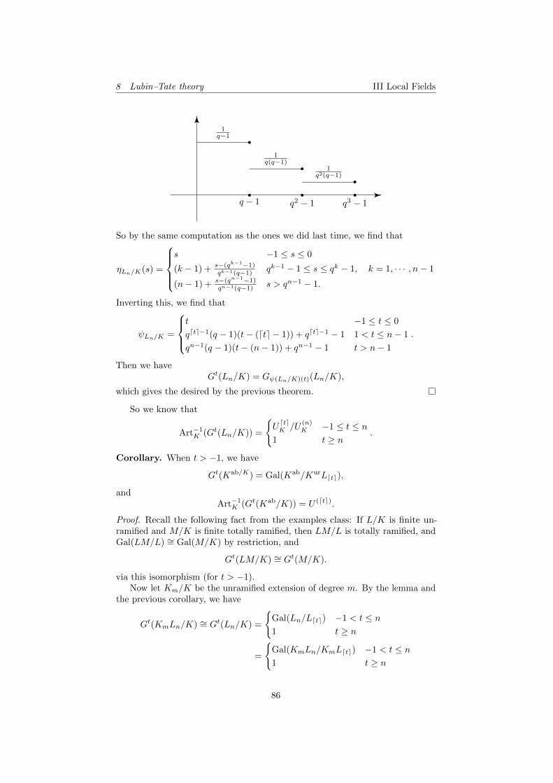
8 Lubin–Tate theory III Local Fields
1q−1
1q(q−1)
1q2(q−1)
q − 1 q2 − 1 q3 − 1
So by the same computation as the ones we did last time, we find that
ηLn/K(s) =
s −1 ≤ s ≤ 0
(k − 1) + s−(qk−1−1)qk−1(q−1)
qk−1 − 1 ≤ s ≤ qk − 1, k = 1, · · · , n− 1
(n− 1) + s−(qn−1−1)qn−1(q−1) s > qn−1 − 1.
Inverting this, we find that
ψLn/K =
t −1 ≤ t ≤ 0
qdte−1(q − 1)(t− (dte − 1)) + qdte−1 − 1 1 < t ≤ n− 1
qn−1(q − 1)(t− (n− 1)) + qn−1 − 1 t > n− 1
.
Then we haveGt(Ln/K) = Gψ(Ln/K)(t)(Ln/K),
which gives the desired by the previous theorem.
So we know that
Art−1K (Gt(Ln/K)) =
{UdteK /U
(n)K −1 ≤ t ≤ n
1 t ≥ n.
Corollary. When t > −1, we have
Gt(Kab/K) = Gal(Kab/KurLdte),
andArt−1
K (Gt(Kab/K)) = U (dte).
Proof. Recall the following fact from the examples class: If L/K is finite un-ramified and M/K is finite totally ramified, then LM/L is totally ramified, andGal(LM/L) ∼= Gal(M/K) by restriction, and
Gt(LM/K) ∼= Gt(M/K).
via this isomorphism (for t > −1).Now let Km/K be the unramified extension of degree m. By the lemma and
the previous corollary, we have
Gt(KmLn/K) ∼= Gt(Ln/K) =
{Gal(Ln/Ldte) −1 < t ≤ n1 t ≥ n
=
{Gal(KmLn/KmLdte) −1 < t ≤ n1 t ≥ n
86

8 Lubin–Tate theory III Local Fields
So we have
Gt(Kab/K) = Gt(KurL∞/K)
= lim←−m,n
Gt(KmLn/K)
= lim←−m,nn≥dte
Gal(KmLn/KmLdte)
= Gal(KurL∞/KurLdte)
= Gal(Kab/KurLdte),
and
Art−1K (Gal(Kab/KurLdte)) = Art−1
K
lim←−m,nn≥dte
Gal(KmLn/KmLdte)
= lim←−
m,nn≥dte
Art−1K
(Gal(KmLn/KmLdte)
)
= lim←−m,nn≥dte
U(dte)K
U(n)K
= Udte.
Corollary. Let M/K be a finite abelian extension. Then we have an isomor-phism
ArtK :K×
N(M/K)∼= Gal(M/K).
Moreover, for t > −1, we have
Gt(M/K) = ArtK
(U
(dte)K N(M/K)
N(M/K)
).
Proof. We have
Gt(M/K) =Gt(Kab/K)G(Kab/M)
G(Kab/M)= Art
(U
(dte)K N(M/K)
N(M/K)
).
87
Index III Local Fields
Index
C(Zp,Qp), 39I-adic completion, 11I-adic topology, 9I-adically complete, 11I-adically open, 9Kur, 66L/K, 52N(L/K), 69
U(s)k , 51
W (M/K), 66W (R), 34ηL/K , 58OK , 15mK , 16πn-division points, 79ψL/K , 60c0, 39iL/K , 55kK , 16p-adic absolute value, 11p-adic integers, 12p-adic numbers, 12sth ramification group, 52x-adic topology, 9
abelian extension, 68absolute ramification index, 36absolute value, 4
archimedean, 5non-archimedean, 5
absolute valuesequivalence, 4
adjoint matrix, 7adjugate matrix, 7algebraic integer, 7archimedean absolute value, 5arithmetic Frobenius, 66
break points, 23
class field, 70Coleman operators, 83
directed system, 64discrete valuation ring, 29discretely valued field, 27DVF, 27
DVR, 29
Eisenstein criterion, 49Eisenstein polynomial, 49equal characteristic, 29equivalence of norm, 19equivalent absolute values, 4
formal additive group, 76formal group, 75
homomorphism, 76module, 77
formal Laurent series, 15formal module, 77formal multiplicative group, 76fundamental theorem of Galois
theory, 65
Galois extension, 63generalized local Kronecker-Weber
theorem, 83geometric Frobenius, 74
Hasse-Arf theorem, 83Hensel’s lemma, 16Herbrand’s theorem, 58Higher ramification groups, 74higher unit groups, 51homomorphism
formal group, 76
inertia degree, 43inertia field, 52inertia group, 52integral element, 7integrally closed, 8inverse limit, 10, 64inverse limit topology, 10inverse system, 64
Krull topology, 63
length, 24line segment, 24local field, 27Local Kronecker-Weber theorem, 74local Kronecker-Weber theorem, 83lower convex hull, 23
88
Index III Local Fields
lower convex set, 23lower numbering of ramification
group, 60Lubin–Tate module, 77Lubin–Tate polynomial, 77Lubin–Tate series, 77
Mahler coefficient, 40Mahler’s theorem, 39maximal ideal, 16mixed characteristic, 29module
formal group, 77multiplicity, 24
Newton polygon, 23non-archimedean absolute value, 5norm
equivalent, 19norm on vector space, 19normal extension, 63normalized valuation, 27
perfect ring, 29primitive polynomial, 16profinite groups, 63projective limit, 10
ramification group, 52lower numbering, 60upper numbering, 60
ramification index, 43rank, 43
residue field, 16ring topology, 9
separable extension, 63slope, 24strict p-ring, 33strong triangle inequality, 5
tame quotient, 55Teichmuller lift, 30Teichmuller map, 30Teichmuller representative, 30topological ring, 9totally ramified extension, 43, 65triangle inequality, 4trivial absolute value, 4
ultrametric, 5uniformizer, 27unramified extension, 43, 65upper numbering of ramification
group, 60
valuation, 15normalized, 27
valuation ring, 7, 15valued field, 4
discretely, 27
Weil group, 66wild inertia group, 55Witt vector, 34
89