PART II OLIGOPOLY

II. 2 COLLUSION

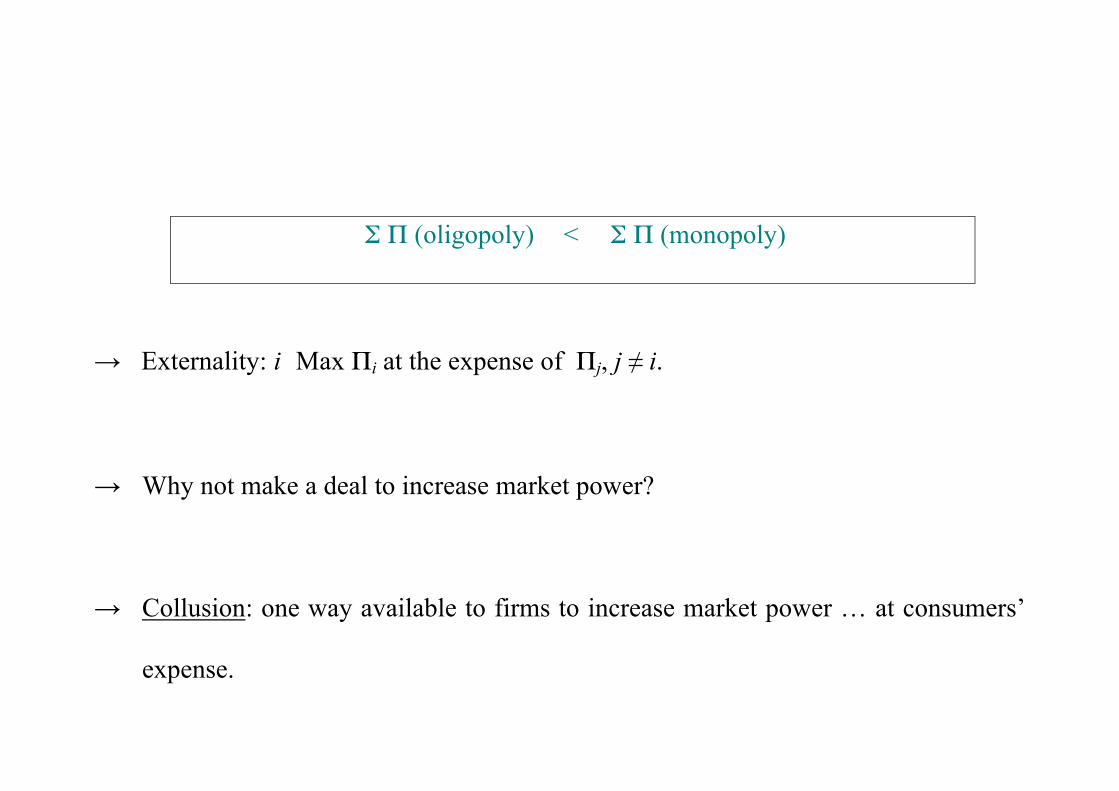
Σ Π (oligopoly) < Σ Π (monopoly)

→ Externality: i Max Πi at the expense of Πj, j ≠  i.

→ Why not make a deal to increase market power?

→ Collusion: one way available to firms to increase market power … at consumers’

expense.

→ * Either official (i.e. cartel)

example : oil price increases in 1973 by OPEC

* Or, more frequently, secret because illegal by the Sherman Act (US) and by

article 85 of the Treaty of Rome (EU).

→ Collusion is frequently a secret agreement either on prices or on quantities (as in

the present chapter).

Instead, firms can also agree on advertising expenses, territory sharing, quality,

etc.

example of territory sharing: the chemical industry in the 20s

ICI → UK & Commonwealth

German firms → continental Europe

Du Pont → America

Illegal since then.

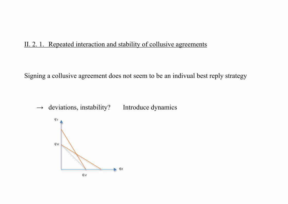
II. 2. 1. Repeated interaction and stability of collusive agreements

Signing a collusive agreement does not seem to be an indivual best reply strategy

→ deviations, instability? Introduce dynamics

qA

qB

qM

qM

The Model

• Cf. Bertrand (duopoly, homogeneous product, constant and symmetric MC, no

capacity constraint)

• Many periods (t = 1, 2, …)

• Firms can change their prices

• Bertrand game at each period: Firms play a repeated game

Equilibrium of such a dynamic game?

• The well-known Nash-Bertrand static equilibrium can be an equilibrium in

this dynamic setting

• There can be other equilibria

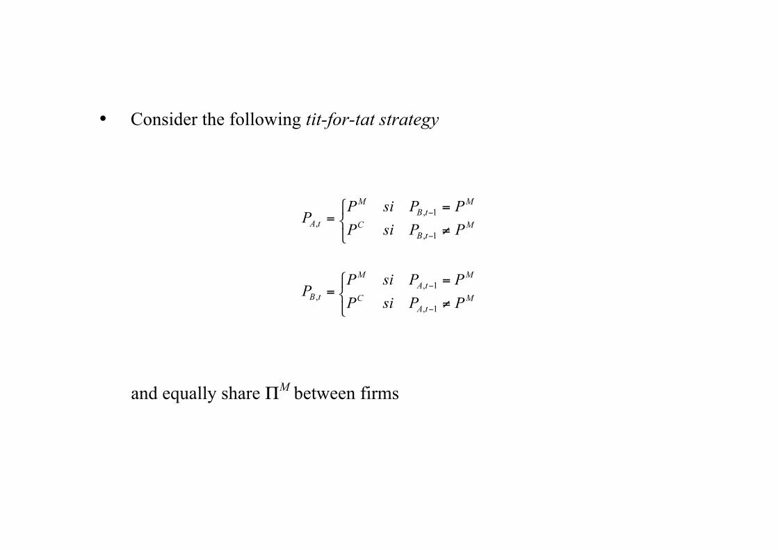
• Consider the following tit-for-tat strategy

and equally share ΠM between firms

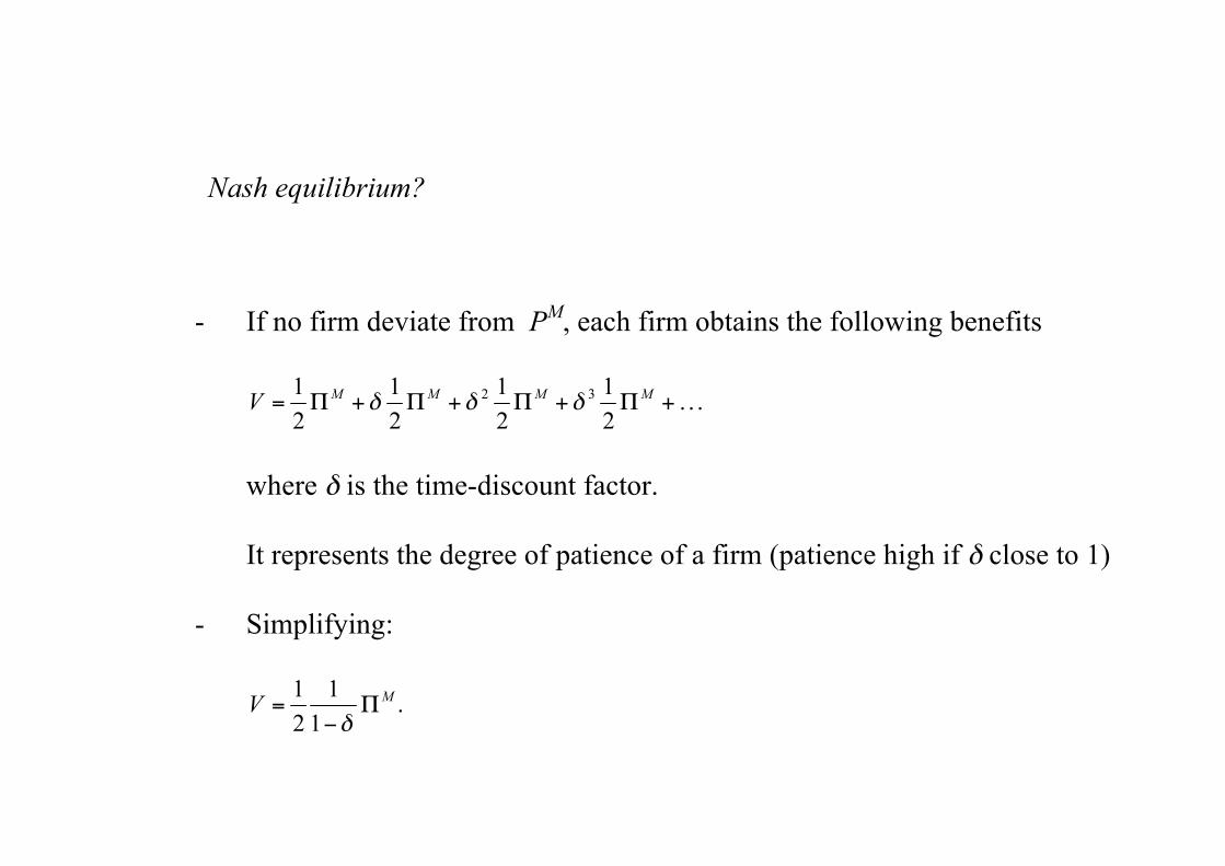
Nash equilibrium?

- If no firm deviate from PM, each firm obtains the following benefits

where δ is the time-discount factor.

It represents the degree of patience of a firm (patience high if δ close to 1)

- Simplifying:

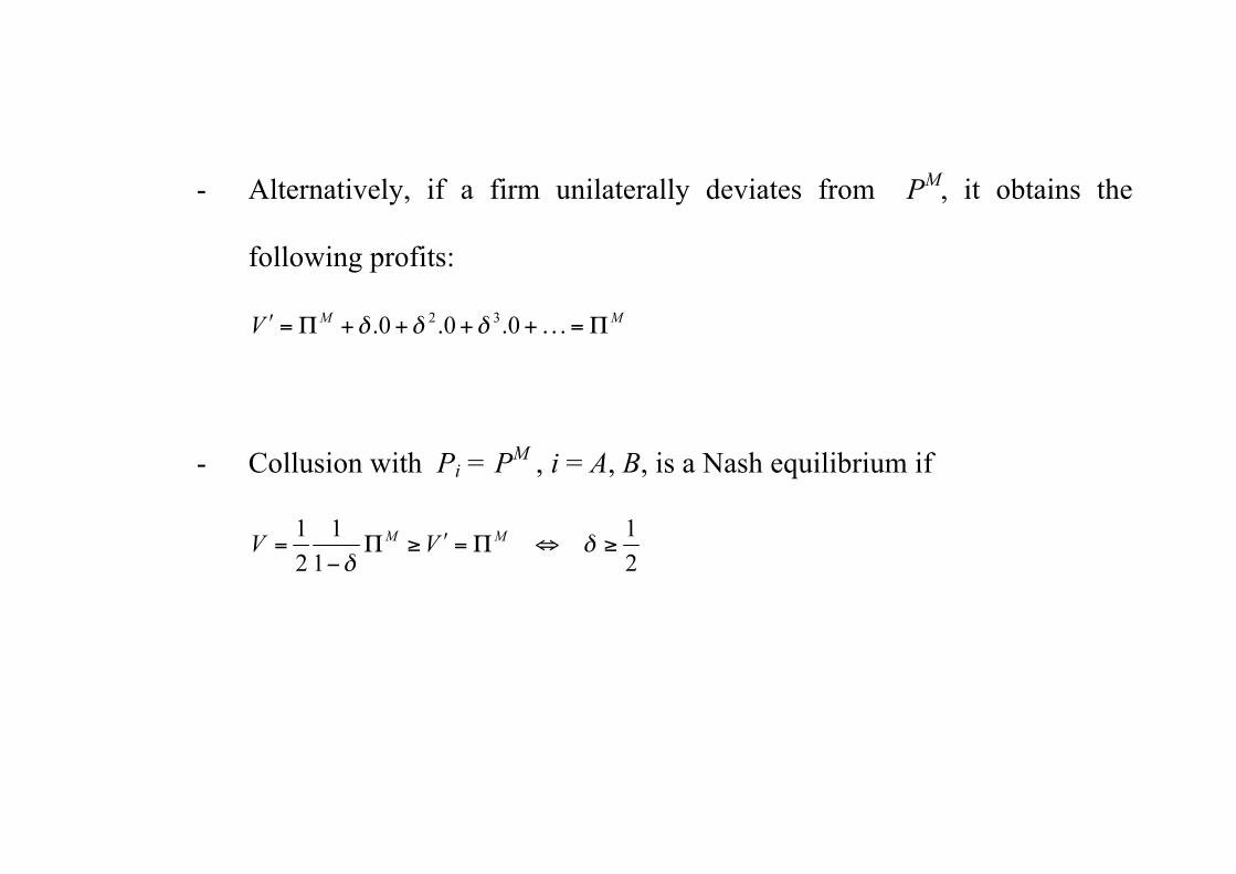
- Alternatively, if a firm unilaterally deviates from PM, it obtains the

following profits:

- Collusion with Pi = PM , i = A, B, is a Nash equilibrium if

- The importance of the discount factor, δ.

It measures what $1 is worth in the future compared with what it is woth

today.

Generally, we assume that 0 < δ < 1.

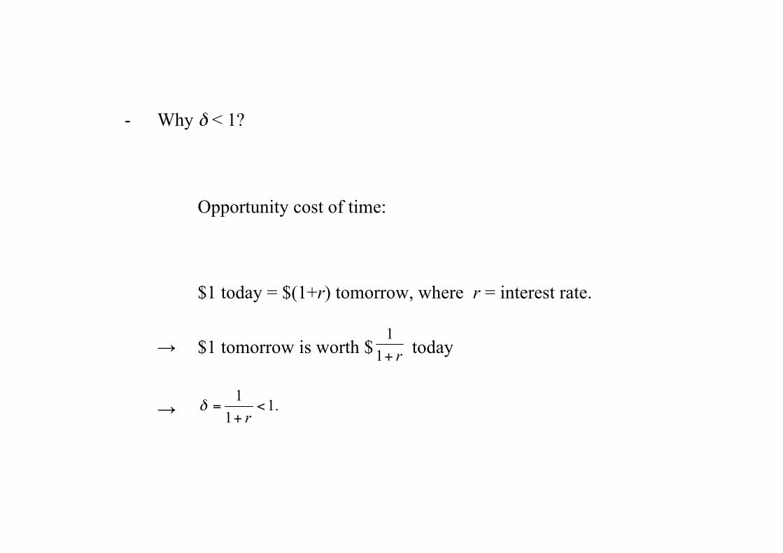
- Why δ < 1?

Opportunity cost of time:

$1 today = $(1+r) tomorrow, where r = interest rate.

→ $1 tomorrow is worth $ today

→

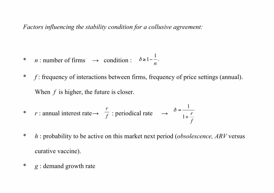
Factors influencing the stability condition for a collusive agreement:

* n : number of firms → condition :

€

δ ≥1− 1n.

* f : frequency of interactions between firms, frequency of price settings (annual).

When f is higher, the future is closer.

* r : annual interest rate → : periodical rate →

* h : probability to be active on this market next period (obsolescence, ARV versus

curative vaccine).

* g : demand growth rate

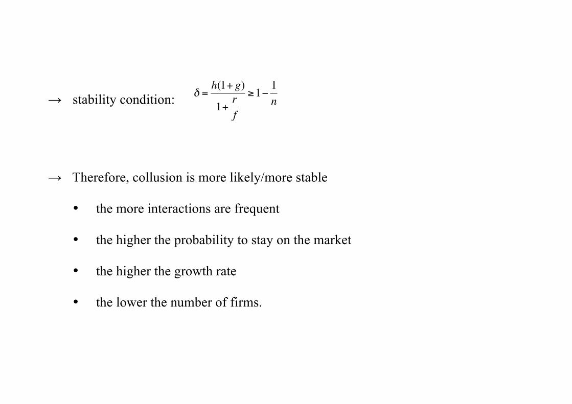
→ stability condition:

€

δ =h(1+ g)

1+rf

≥1− 1n  

→ Therefore, collusion is more likely/more stable

• the more interactions are frequent

• the higher the probability to stay on the market

• the higher the growth rate

• the lower the number of firms.

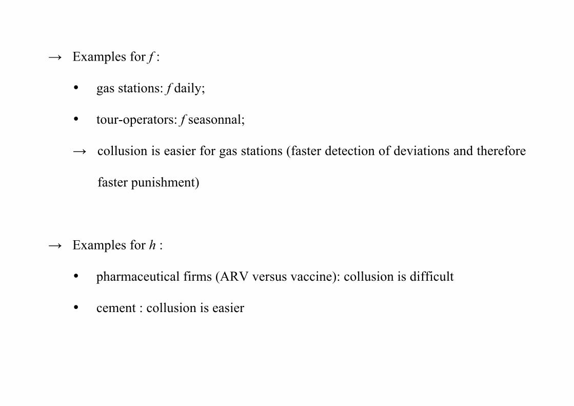
→ Examples for f :

• gas stations: f daily;

• tour-operators: f seasonnal;

→ collusion is easier for gas stations (faster detection of deviations and therefore

faster punishment)

→ Examples for h :

• pharmaceutical firms (ARV versus vaccine): collusion is difficult

• cement : collusion is easier

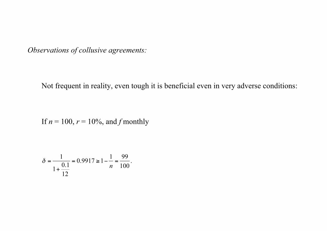
Observations of collusive agreements:

Not frequent in reality, even tough it is beneficial even in very adverse conditions:

If n = 100, r = 10%, and f monthly

Why?

• It is illegal;

• High turnover (low h) ;

• Collusive strategy that implies a permanent price war. However, all firms are

better of revising their strategies over time, it is not renegotiation-proof.

Therefore, the threat of a price war is not credible.

• When it is difficult to observe prices, secret deviations are possible and the

collusive agreement is less stable.

To sum up

What matters for the stability of the collusive agreement is the trade-off short-term

gains and long-term losses.

II. 2. 2. Price wars

Observation

Industry prices oscillate between high levels and low levels.

→ Contradicts the collusive stability condition

→ Extensions of the model

Secret price cuts and demand flucuations

Markets with huge clients (concrete or ships), negotiated prices, difficult to

identify price cuts.

Model 1

Each firm only observes its own demand, not the total demand.

If a firm’s demand is low, either its rival has secretly decreased its price, or the

total demand is low.

→ Punishment? (bad equilibrium)

or not? (bad incentive).

→ temporary price wars and pro-cyclical prices.

Model 2

Each firm observes total demand.

Gains from deviations are higher the larger the total demand.

→ A collusive agreement should specify common price decreases in periods of

high demand to desincentivate unilateral deviations (the gains associated to a

deviation are lower if prices decrease).

→ Counter-cyclical prices.

Empirically,

Both models seem relevant, depending on the sectors under analysis:

• Cement prices between 1947 and 1981 : counter-cyclical

• Ships built in Chicago the East Coast: pro-cyclical prices

II. 2. 3. An additional factor that eases collusion

• Multi-markets contacts.