How Much Collusion? A Meta-Analysis On Oligopoly Experiments

MAX PLANCK SOC IETY

Preprints of theMax Planck Institute for

Research on Collective GoodsBonn 2006/27

How Much Collusion?A Meta-Analysis On Oligopoly Experiments

Christoph Engel

Preprints of the Max Planck Institute for Research on Collective Goods Bonn 2006/27

How Much Collusion? A Meta-Analysis On Oligopoly Experiments

Christoph Engel

December 2006

Max Planck Institute for Research on Collective Goods, Kurt-Schumacher-Str. 10, D-53113 Bonn http://www.coll.mpg.de

1

Christoph Engel

How Much Collusion? A Meta-Analysis On Oligopoly Experiments

I. Research Question 2 II. Methodology 3 III. Dependence of Collusion on Product Characteristics 7

1. Homogeneity vs. Heterogeneity of Goods 7 2. Effect of Introducing Fixed Costs 10 3. Effect of Constrained Capacity 10 4. Effect of Advance Production 12 5. Collusion when Process Innovation in Possible 13

IV. Dependence of Collusion on Market Characteristics 14 1. Effect of Market Size 14 2. Symmetry vs. Asymmetry of Sellers 17 3. Effect of Power Asymmetries among Sellers 19

V. Dependence of Collusion on Demand and Supply Characteristics 20 1. Effect of Demand Characteristics 20 2. Effect of Supply Characteristics 21 3. Dependence of Collusion on the Distribution of the Surplus 22

VI. Dependence of Collusion on Seller Characteristics 23 VII. Role of Seller Interaction in Explaining Collusion 24

1. Dependence on the Strategic Variable 24 2. Simultaneous vs. Sequential Interaction 26 3. Duration of the Interaction between Sellers 27 4. Partner vs. Stranger Design 29 5. Effect of Communication on Collusion 31 6. Option to Agree 33

VIII.Dependence of Collusion on the Information Environment 36 1. Role of Ex Ante Information 36 2. Role of Feedback 39 3. Neutral vs. Market Frame 42

IX. Sensitivity of Collusion to Buyer Activity 43 1. Computer vs. Human Buyers 43 2. Sensitivity of Collusion to the Trading Institution 43 3. Collusion under Conditions of Demand Inertia 45

X. Conclusion 46 * I am grateful to Werner Güth, Reinhard Selten, Martin Hellwig, Martin Beckenkamp,

Thomas Gaube and Frank Maier-Rigaud for their advice, and to Lena Heuner for her help in tracing old papers.

2

I. Research Question

Richness can be embarrassing. Oligopoly has been among the first topics in experimental eco-nomics, starting as early as 1959 (Hoggatt 1959; Selten and Sauermann 1959). In the meantime, a total of 154 experimental papers has been published1. Many of them report on more than one experiment, so that there is data on much more than 500 different parameter constellations2. There is a number of survey articles (Friedman 1969; Plott 1982; Plott 1989; Davis and Holt 1993; Holt 1995; Lupi and Sbriglia 2003; Huck, Normann et al. 2004; Suetens 2004; Suetens and Potters 2005). But the latest comprehensive survey is a decade old. Moreover, it does not make the findings comparable across publications. This is undertaken in the present meta-study. It uses a simple question to turn the richness of the material into a boon: how much collusion have the respective experimenters found? More than one would normatively want? And more than game theory would expect?

Specifically, this study not only compares what experimenters have set out to test. In order to test subjects on their respective research question, they had to specify a whole array of other parame-ters, like product characteristics, market size, the shape of supply and demand, the strategic vari-able, the duration of the game, communication protocols, the information environment, and trad-ing institutions. That way they have generated a rich body of data that has remained untapped thus far. This meta-study makes this data available.

This richness of the data has a third advantage. The sample is large enough to make many inter-action effects significant. The most important ones are presented here.

Actually, these questions are not only helpful in generating order. They are also decisive for the main users of oligopoly experiments: the antitrust authorities. There are two main ways how these authorities may put experimental findings to productive use. Even in legal orders as dedi-cated to antitrust enforcement as the US, the European Community or Germany, administrative resources are limited. Knowing which factors facilitate collusion most helps these authorities detect instances of collusion.

Yet the relevance is not confined to administrative policy. Getting the expected degree of collu-sion right also matters in doctrinal terms. Both in the US3 and in Europe,4 merger control inter-venes if the fact that a previously independent commercial entity disappears from the market makes “tacit collusion“ substantially more likely. The behavioural evidence helps antitrust au-thorities in their ensuing predictive task. For them, understanding interaction effects is particu-

1 For references see the list at the end of this paper. 2 For the reasons laid out in section II, this study covers 510 independent observations. 3 Department of Justice, Federal Trade Commission, Antitrust Division, 1992 Horizontal Merger Guidelines

of September 10, 1992, 57 FR 41552, Section 2.1. 4 Court of First Instance, 6 June 2002, Airtours plc v Commission of the European Communities, European

Court Reports 2002 II 2585, at para. 60; Guidelines on the Assessment of Horizontal Mergers under the Council Regulation on the Control of Concentrations between Undertakings, OJ 2004 C 31/5, para. 22, 39, 41

3

larly relevant. They have to find out whether the co-presence of two or more factors makes it more or less likely that collusion happens.

The remainder of this article is organised as follows. Section II specifies the methodology. Sec-tion III presents the evidence on product characteristics. Section IV addresses market structure, section V supply and demand, section VI seller characteristics, section VII seller interaction, sec-tion VIII the information environment, and section IX buyer activity. Section X concludes.

II. Methodology

Individual experimental papers often excel in sophistication. They for instance offer complex theoretical models for explaining the data. Recently, a wealth of learning theories has been used for the purpose (see in particular Sherman 1969; Shubik, Wolf et al. 1971; Cox and Walker 1998; Nagel and Vriend 1999b; Nagel and Vriend 1999a; Rassenti, Reynolds et al. 2000; Capra, Goeree et al. 2002; Offerman, Potters et al. 2002; Anderhub, Güth et al. 2003; Bosch-Domènech and Vriend 2003; Altavilla, Luini et al. 2005). Others present demanding statistical models (e.g. Daughety and Forsythe 1987; Benson and Faminow 1988; Davis, Reilly et al. 2003; Davis and Wilson 2005). Most papers give graphical information on time series. None of this works for a study that aims at being as encompassing as possible. The reason is simple. Many publications do not offer the data one would need for the purpose.

One information, however, is hardly ever missing: which has been the effect of the respective treatment on the strategic variable of the oligopolists (which is normally either price or quan-tity)? Specifically, in the large majority of papers, this information is given per instance of inter-action. If the author has not done so anyhow, it is easy to calculate the mean for all rounds of interaction. Of course, duration matters. In a typical experiment, there is a pronounced change from the initial rounds over the middle of the game towards end effects (Selten and Stoecker 1986). If one adds many more rounds, the characteristic picture may reverse (Alger 1987). But duration varies so profoundly from experiment to experiment that only comparing aggregates is feasible. Since the number of rounds from which the mean is taken is always reported, one may control the result for total duration.

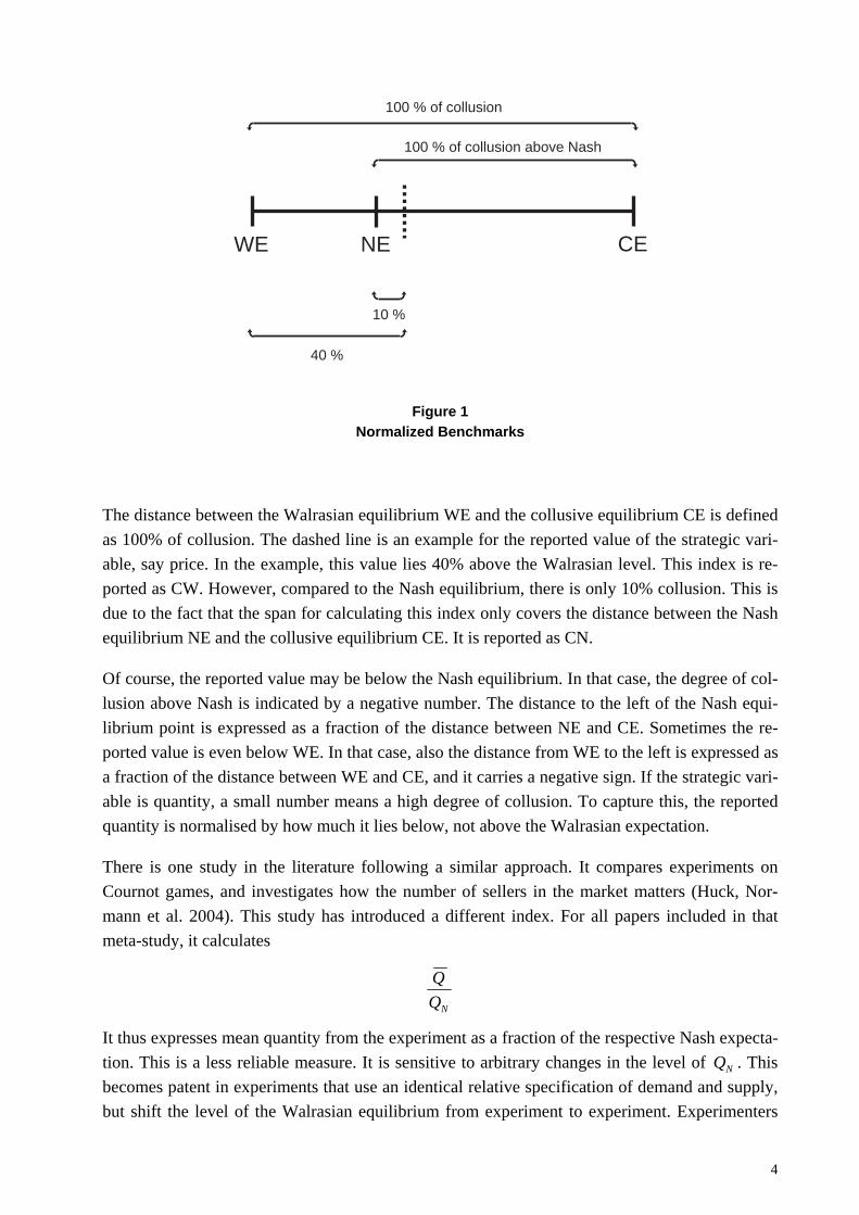
Absolute price or quantity is not meaningful across experiments. One needs a standardised benchmark. Actually, in oligopoly games there are three such benchmarks: the Walrasian and the collusive benchmarks always exist. In the standard Bertrand situation, the Walrasian and the Nash benchmark coincide (Bertrand 1883). But when marginal cost is not constant, or when firms compete in quantity, to name only the two most important reasons, the Nash equilibrium predicts a different outcome. Typically, it is between the Walrasian and the collusive expecta-tions. This makes for the following picture.

4

WE NE CE

100 % of collusion

10 %

40 %

100 % of collusion above Nash

Figure 1 Normalized Benchmarks

The distance between the Walrasian equilibrium WE and the collusive equilibrium CE is defined as 100% of collusion. The dashed line is an example for the reported value of the strategic vari-able, say price. In the example, this value lies 40% above the Walrasian level. This index is re-ported as CW. However, compared to the Nash equilibrium, there is only 10% collusion. This is due to the fact that the span for calculating this index only covers the distance between the Nash equilibrium NE and the collusive equilibrium CE. It is reported as CN.

Of course, the reported value may be below the Nash equilibrium. In that case, the degree of col-lusion above Nash is indicated by a negative number. The distance to the left of the Nash equi-librium point is expressed as a fraction of the distance between NE and CE. Sometimes the re-ported value is even below WE. In that case, also the distance from WE to the left is expressed as a fraction of the distance between WE and CE, and it carries a negative sign. If the strategic vari-able is quantity, a small number means a high degree of collusion. To capture this, the reported quantity is normalised by how much it lies below, not above the Walrasian expectation.

There is one study in the literature following a similar approach. It compares experiments on Cournot games, and investigates how the number of sellers in the market matters (Huck, Nor-mann et al. 2004). This study has introduced a different index. For all papers included in that meta-study, it calculates

NQQ

It thus expresses mean quantity from the experiment as a fraction of the respective Nash expecta-tion. This is a less reliable measure. It is sensitive to arbitrary changes in the level of NQ . This becomes patent in experiments that use an identical relative specification of demand and supply, but shift the level of the Walrasian equilibrium from experiment to experiment. Experimenters

5

sometimes have done so in order to exclude parameter learning (for an example see Isaac, Ramey et al. 1984)5. Moreover, this index generates high values if NQ is very small, and low values if NQ is very high in absolute terms. And it cannot be calculated if an experimenter has normalised 0=NQ . For three reasons, this index is nonetheless calculated wherever possible. It is reported as NN. First it makes comparisons easier with the (small) set of papers in the litera-ture that presents this index. Occasionally the CN index suffers from a mirror problem. If the Nash equilibrium is close to the collusive equilibrium, this index grows very large. In the ex-periments covered by this study, however, this is a rare event. Most importantly, however, there are several treatment variables where the NN index is significant, while the CN index is not.

60 of the 510 experiments covered in this study use a stranger design. In every round, subjects are rematched. Behaviourally speaking, this is not the same as one-shot interaction. From round 2 on, subjects come with the expectations built in previous rounds. But it at least is as good an approximation as is feasible with the experimental method. In the remaining 460 experiments, however, interaction is repeated. As is known from the folk theorem, this leads to multiple Nash equilibria if there is uncertainty about the end of the game (Aumann and Shapley 1994). Of course, the data on repetition effects is reported here. However, for calculating the Nash bench-mark, repetition is ignored. The benchmark is always taken from the one-shot game.

The large majority of the experiments covered in this study use a computer to simulate the oppo-site market side. This computer is programmed as a non-strategic actor. It simply represents the demand curve. Equilibrium analysis becomes much more demanding if there are strategic actors on both sides of the market. In order to make the data comparable across treatments, this element of the situation is ignored when calculating the Nash equilibrium in the minority of experiments with human buyers. The benchmark is always exclusively taken from the interaction between sellers, i.e. assuming passive buyers.

The number of papers which themselves calculate one of the three indices is very small (see e.g. Cason and Davis 1995). But generating them is straightforward if the benchmarks and the means are reported. This, however, is often not the case. Whenever possible, these calculations have been done in preparation of this meta-study. Often this meant optimisation calculus. If the Wal-rasian benchmark was missing, often the industry demand and supply functions had to be con-structed from firm functions, or directly from the cost functions. Occasionally, the reported val-ues had to be weighted for calculating the means, for instance if discrete outcomes had different frequencies. The data bank behind this paper specifies which parameters could not be taken di-rectly from the respective paper, and it explains which kind of judgement has been exercised in so doing, if necessary. It is publicly available.

Following the theory of induced valuation (Smith 1976), in the Seventies and Eighties, many experimenters have given their subjects step functions for supply and demand. Determining the

5 Take the following simple example: in the first experiment, WE = 0, CE = 100, NE = 50, experimental data

40. In this case, the index is 40/50 = 0,8. Now shift the scale by 100, leaving relative positions unaffected. Now WE = 100, CE = 200, NE = 150, experimental data 140. Now the index is 140/150 = 0,9333.

6

Walrasian equilibrium is straightforward with step functions. It is the point where the two step functions cross. Calculating the collusive equilibrium requires trial and error, but is doable. However, since these functions are characterised by discontinuities, there is often no Nash equi-librium in pure strategies. Calculating the mixed equilibria is theoretically possible, but it is a formidable task (Holt and Solis-Soberon 1992). If the authors themselves have done so, and if they have come up with a single equilibrium, the expected value is taken as the Nash benchmark. But the effort for doing so for all the remaining papers with step functions would have been pro-hibitive. Instead, it is only checked whether there is a Nash equilibrium in pure strategies (at or directly above the Walrasian equilibrium). If this is not the case, the two indices relying on the Nash equilibrium are left blank. This is the main, but not the only reason why it has not been possible for all papers to calculate all three indices. The databank specifies which indices are missing, and for which reason. In the presentation of the results, for each index the composition of the sample is presented separately.

47 papers have a pertinent topic, but are not included in this meta-study. There are different rea-sons for excluding them. Most frequently, in the paper there are only graphs, but no exact num-bers for calculating the means. In other cases, it is not possible to calculate the benchmarks, for instance because a step function is only presented graphically and measurement scales cannot be reconstructed from the graph. Sometimes, the research question is too far away, for instance if the experimenters have given their subjects so little information that it is meaningless to talk about collusion. Finally, some papers do not give summary statistics, but exclusively regressions, and the model is such that the data relevant for this comparative paper cannot be reconstructed. Also, experiments on spatial competition are excluded.

The data is presented the following way. The main effect of each treatment variable is calculated three times. The first calculation covers all experiments with the respective feature. It is called the gross data. Some papers do not report the standard variable. They for instance do not indicate industry profit, or the necessary elements for calculating it, when sellers are asymmetric. In such cases, the best available proxy is taken for calculating the indices.6 Other papers do not give data for all rounds of repetition, but only for some of them. Such somehow unusual data is excluded from the second calculation. It is called ordinary coverage. Finally, the effect is calculated a third time with data taken only from those experiments where this was a treatment variable. This is called the treatment data.

All effects are tested for significance by way of ANOVA. That way, interaction effects can be analysed as well. The samples are relatively large. However, variance might not always be ho-mogeneous in subsamples. Moreover, the number of cases in each subsample is not always bal-anced. For both reasons, ANOVA results might not be fully reliable (see Hays 1994:10.20). Therefore, as a double-check, the main effects are also tested with a non parametric test.7 If the independent variable is dichotomous, a Mann Whitney U Test is used. If the independent vari-

6 The respective proxy is specified in the data bank. 7 Reinhard Selten had suggested to do so.

7

able has more than two categories, a Kruskal Wallis test is applied (as suggested by Bortz 2005:287). In most cases, the p-values are similar. Not so rarely, the non parametric test even yields a smaller p-value than the ANOVA.

In order to save space, insignificant findings are not presented. Weakly significant findings (p<0,1) are reported where the result seems sufficiently relevant. The treatment data, however, is always reported. This is justified since experimenters themselves had to check for significance. The results of the non parametric test are only presented if the ANOVA has yielded a significant result.

III. Dependence of Collusion on Product Characteristics

1. Homogeneity vs. Heterogeneity of Goods

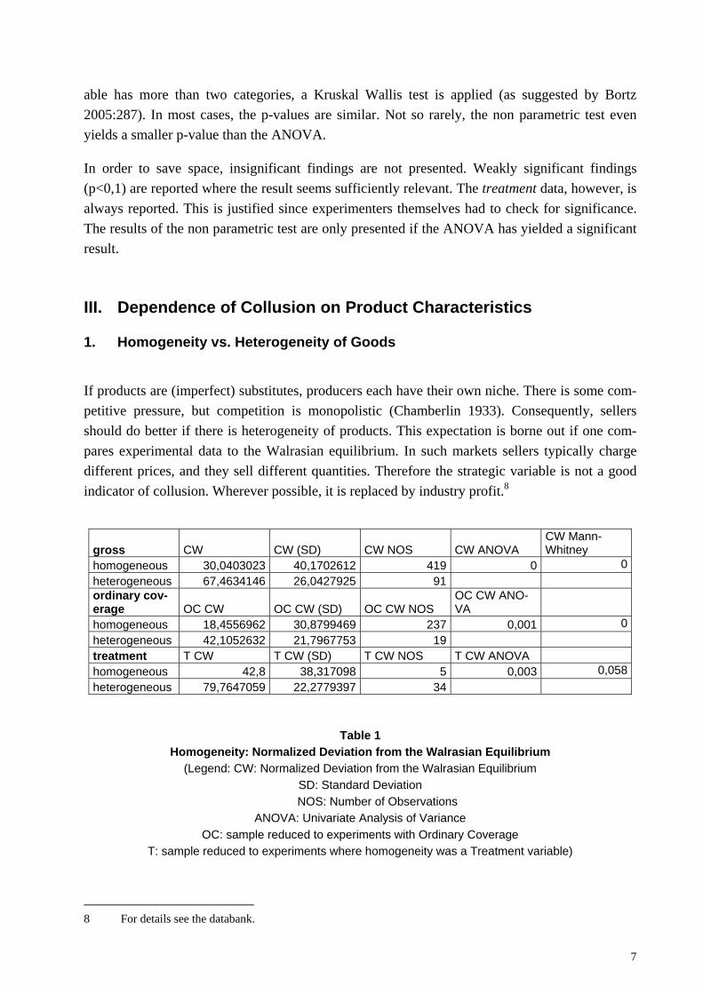
If products are (imperfect) substitutes, producers each have their own niche. There is some com-petitive pressure, but competition is monopolistic (Chamberlin 1933). Consequently, sellers should do better if there is heterogeneity of products. This expectation is borne out if one com-pares experimental data to the Walrasian equilibrium. In such markets sellers typically charge different prices, and they sell different quantities. Therefore the strategic variable is not a good indicator of collusion. Wherever possible, it is replaced by industry profit.8

gross CW CW (SD) CW NOS CW ANOVA CW Mann-Whitney

homogeneous 30,0403023 40,1702612 419 0 0heterogeneous 67,4634146 26,0427925 91 ordinary cov-erage OC CW OC CW (SD) OC CW NOS

OC CW ANO-VA

homogeneous 18,4556962 30,8799469 237 0,001 0heterogeneous 42,1052632 21,7967753 19 treatment T CW T CW (SD) T CW NOS T CW ANOVA homogeneous 42,8 38,317098 5 0,003 0,058heterogeneous 79,7647059 22,2779397 34

Table 1 Homogeneity: Normalized Deviation from the Walrasian Equilibrium

(Legend: CW: Normalized Deviation from the Walrasian Equilibrium SD: Standard Deviation

NOS: Number of Observations ANOVA: Univariate Analysis of Variance

OC: sample reduced to experiments with Ordinary Coverage T: sample reduced to experiments where homogeneity was a Treatment variable)

8 For details see the databank.

8

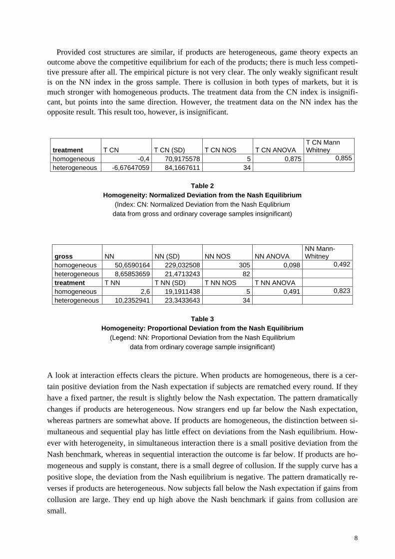
Provided cost structures are similar, if products are heterogeneous, game theory expects an outcome above the competitive equilibrium for each of the products; there is much less competi-tive pressure after all. The empirical picture is not very clear. The only weakly significant result is on the NN index in the gross sample. There is collusion in both types of markets, but it is much stronger with homogeneous products. The treatment data from the CN index is insignifi-cant, but points into the same direction. However, the treatment data on the NN index has the opposite result. This result too, however, is insignificant.

treatment T CN T CN (SD) T CN NOS T CN ANOVA T CN Mann Whitney

homogeneous -0,4 70,9175578 5 0,875 0,855heterogeneous -6,67647059 84,1667611 34

Table 2

Homogeneity: Normalized Deviation from the Nash Equilibrium (Index: CN: Normalized Deviation from the Nash Equlibrium

data from gross and ordinary coverage samples insignificant)

gross NN NN (SD) NN NOS NN ANOVA NN Mann-Whitney

homogeneous 50,6590164 229,032508 305 0,098 0,492heterogeneous 8,65853659 21,4713243 82 treatment T NN T NN (SD) T NN NOS T NN ANOVA homogeneous 2,6 19,1911438 5 0,491 0,823heterogeneous 10,2352941 23,3433643 34

Table 3

Homogeneity: Proportional Deviation from the Nash Equilibrium (Legend: NN: Proportional Deviation from the Nash Equilibrium

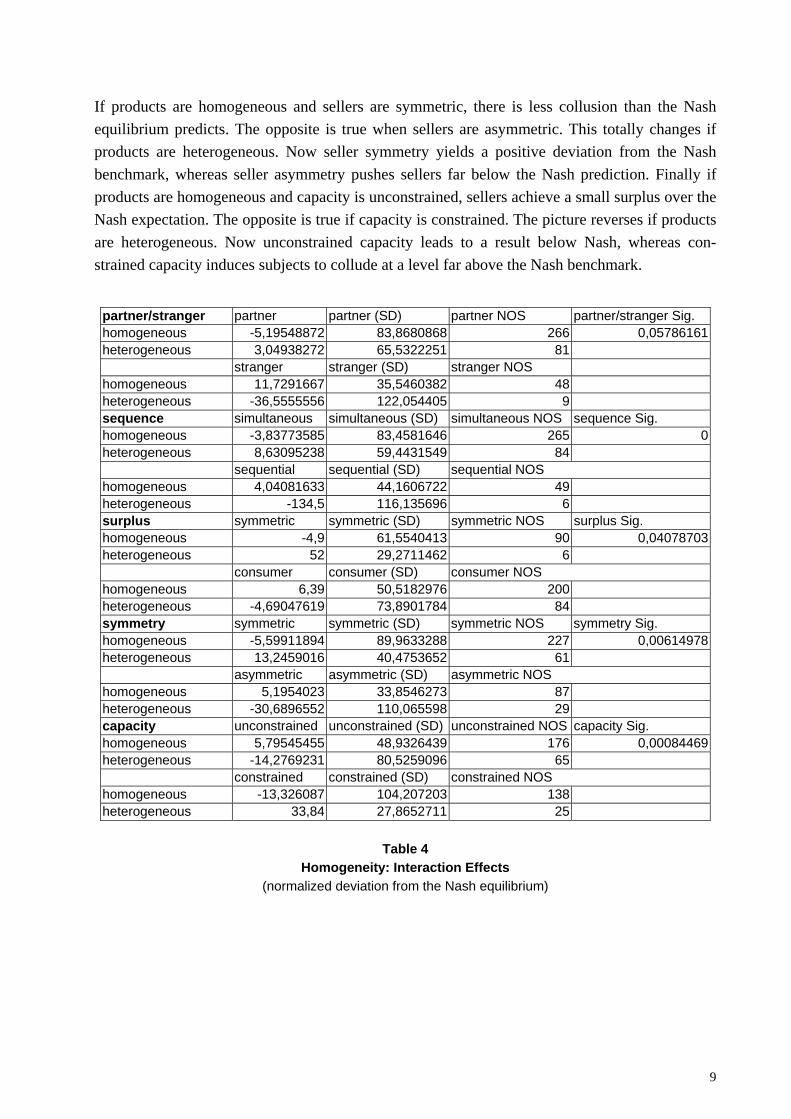
data from ordinary coverage sample insignificant) A look at interaction effects clears the picture. When products are homogeneous, there is a cer-tain positive deviation from the Nash expectation if subjects are rematched every round. If they have a fixed partner, the result is slightly below the Nash expectation. The pattern dramatically changes if products are heterogeneous. Now strangers end up far below the Nash expectation, whereas partners are somewhat above. If products are homogeneous, the distinction between si-multaneous and sequential play has little effect on deviations from the Nash equilibrium. How-ever with heterogeneity, in simultaneous interaction there is a small positive deviation from the Nash benchmark, whereas in sequential interaction the outcome is far below. If products are ho-mogeneous and supply is constant, there is a small degree of collusion. If the supply curve has a positive slope, the deviation from the Nash equilibrium is negative. The pattern dramatically re-verses if products are heterogeneous. Now subjects fall below the Nash expectation if gains from collusion are large. They end up high above the Nash benchmark if gains from collusion are small.

9

If products are homogeneous and sellers are symmetric, there is less collusion than the Nash equilibrium predicts. The opposite is true when sellers are asymmetric. This totally changes if products are heterogeneous. Now seller symmetry yields a positive deviation from the Nash benchmark, whereas seller asymmetry pushes sellers far below the Nash prediction. Finally if products are homogeneous and capacity is unconstrained, sellers achieve a small surplus over the Nash expectation. The opposite is true if capacity is constrained. The picture reverses if products are heterogeneous. Now unconstrained capacity leads to a result below Nash, whereas con-strained capacity induces subjects to collude at a level far above the Nash benchmark.

partner/stranger partner partner (SD) partner NOS partner/stranger Sig. homogeneous -5,19548872 83,8680868 266 0,05786161heterogeneous 3,04938272 65,5322251 81

stranger stranger (SD) stranger NOS homogeneous 11,7291667 35,5460382 48 heterogeneous -36,5555556 122,054405 9 sequence simultaneous simultaneous (SD) simultaneous NOS sequence Sig. homogeneous -3,83773585 83,4581646 265 0heterogeneous 8,63095238 59,4431549 84

sequential sequential (SD) sequential NOS homogeneous 4,04081633 44,1606722 49 heterogeneous -134,5 116,135696 6 surplus symmetric symmetric (SD) symmetric NOS surplus Sig. homogeneous -4,9 61,5540413 90 0,04078703heterogeneous 52 29,2711462 6

consumer consumer (SD) consumer NOS homogeneous 6,39 50,5182976 200 heterogeneous -4,69047619 73,8901784 84 symmetry symmetric symmetric (SD) symmetric NOS symmetry Sig. homogeneous -5,59911894 89,9633288 227 0,00614978heterogeneous 13,2459016 40,4753652 61

asymmetric asymmetric (SD) asymmetric NOS homogeneous 5,1954023 33,8546273 87 heterogeneous -30,6896552 110,065598 29 capacity unconstrained unconstrained (SD) unconstrained NOS capacity Sig. homogeneous 5,79545455 48,9326439 176 0,00084469heterogeneous -14,2769231 80,5259096 65

constrained constrained (SD) constrained NOS homogeneous -13,326087 104,207203 138 heterogeneous 33,84 27,8652711 25

Table 4

Homogeneity: Interaction Effects (normalized deviation from the Nash equilibrium)

10

2. Effect of Introducing Fixed Costs

All three benchmarks for this study are taken from the one-shot situation. On the short run, for rational actors only marginal, and hence variable cost should matter. However, subjects interact over multiple rounds, and if there is a fixed cost it matters for the payment they expect from the experimenter. One should therefore expect that subjects trade at a price further away from the Walrasian equilibrium if there is a fixed cost. This expectation holds true in the data from the gross sample. In line with this, with no fixed cost, the normalised mean deviation from the Nash equilibrium is negative. If there is a fixed cost, the mean deviation becomes positive. Apparently, subjects do not decide in a purely forward-looking manner.


no fixed cost 32,2363184 36,2569986 408 0 0fixed cost 58,4285714 53,5142452 102

Table 5

Fixed Cost: Normalized Deviation from the Walrasian Equilibrium (data on ordinary coverage insignificant; no treatment data available)

gross CN CN (SD) CN NOS CN ANOVA CN Mann-Whitney

no fixed cost -6,76489028 77,7691586 319 0,022 0fixed cost 14,7882353 73,6943647 85

Table 6

Fixed Cost: Normalized Deviation from the Nash Equilibrium (data on ordinary coverage insignificant; no treatment data available

data on NN index from gross and ordinary coverage samples insignificant, from treatment sample not available)

3. Effect of Constrained Capacity

If sellers compete in price, if products are homogeneous, and if marginal cost is constant, the mere presence of a second seller suffices to force the competitive equilibrium on the sellers. This is in essence the result of (Bertrand 1883). In the literature, this result is typically referred to as the “Bertrand paradox“ (e.g. Tirole 1988:210). Among the many attempts to dissolve the para-dox, the first had been to introduce capacity constraints (Edgeworth 1897). Theory then expects positive profits. The experimental data stands in harsh opposition to the expectation. If capacity is constrained, collusion plummets with respect to all three indices.

11


unconstrained 54,0912698 38,9772076 252 0 0constrained 16,8590308 32,7397548 227 ordinary cov-erage OC CW OC CW (SD) OC CW NOS

OC CW ANO-VA

unconstrained 42,5 24,2806826 98 0 0constrained 6,38607595 26,1501604 158

Table 7

Capacity: Normalized Deviation from the Walrasian Equilibrium (no treatment data available)


unconstrained 0,38174274 59,6220345 241 0,41 0,769constrained -6,09202454 97,9236166 163 ordinary cov-erage OC CN OC CN (SD) OC CN NOS

OC CN ANO-VA

unconstrained 5,64516129 33,9112157 93 0,028 0constrained -20,2340426 107,531583 94

Table 8

Capacity: Normalized Deviation from the Nash Equilibrium (no treatment data available)


unconstrained 58,1631799 252,777783 239 0,044 0,421constrained 15,2702703 70,1011509 148 ordinary cov-erage OC NN OC NN (SD) OC NN NOS

OC NN ANO-VA

unconstrained 130,43956 396,327031 91 0,004 0,001constrained 5,625 74,1055961 88

Table 9

Capacity: Proportional Deviation from the Nash Equilibrium (no treatment data available)

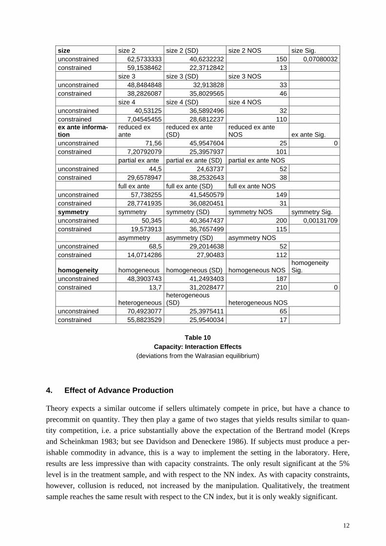
Interaction effects make it possible to say more about the underlying forces. Most graphic is the interaction with market size. In duopoly, the constraint only has a small (negative) effect on the deviation from the Walrasian equilibrium. The effect becomes a bit more pronounced in triopoly, and is strong in larger markets. In asymmetric markets, the negative effect of a capacity con-straint on deviations from the Walrasian equilibrium is much more pronounced than in symmet-ric markets. Likewise, the negative effect is stronger in sequential than in simultaneous interac-tion. Collusion in homogeneous markets is dampened much more by a capacity constraint than when subjects trade in substitutes. Finally, a capacity constraint reduces collusion with all speci-fications of ex ante information, but the reduction is much stronger with reduced ex ante infor-mation.

12

size size 2 size 2 (SD) size 2 NOS size Sig. unconstrained 62,5733333 40,6232232 150 0,07080032constrained 59,1538462 22,3712842 13 size 3 size 3 (SD) size 3 NOS unconstrained 48,8484848 32,913828 33 constrained 38,2826087 35,8029565 46 size 4 size 4 (SD) size 4 NOS unconstrained 40,53125 36,5892496 32 constrained 7,04545455 28,6812237 110 ex ante informa-tion

reduced ex ante

reduced ex ante (SD)

reduced ex ante NOS ex ante Sig.

unconstrained 71,56 45,9547604 25 0constrained 7,20792079 25,3957937 101 partial ex ante partial ex ante (SD) partial ex ante NOS unconstrained 44,5 24,63737 52 constrained 29,6578947 38,2532643 38 full ex ante full ex ante (SD) full ex ante NOS unconstrained 57,738255 41,5450579 149 constrained 28,7741935 36,0820451 31 symmetry symmetry symmetry (SD) symmetry NOS symmetry Sig. unconstrained 50,345 40,3647437 200 0,00131709constrained 19,573913 36,7657499 115 asymmetry asymmetry (SD) asymmetry NOS unconstrained 68,5 29,2014638 52 constrained 14,0714286 27,90483 112

homogeneity homogeneous homogeneous (SD) homogeneous NOS homogeneity Sig.

unconstrained 48,3903743 41,2493403 187 constrained 13,7 31,2028477 210 0

heterogeneousheterogeneous (SD) heterogeneous NOS

unconstrained 70,4923077 25,3975411 65 constrained 55,8823529 25,9540034 17

Table 10

Capacity: Interaction Effects (deviations from the Walrasian equilibrium)

4. Effect of Advance Production

Theory expects a similar outcome if sellers ultimately compete in price, but have a chance to precommit on quantity. They then play a game of two stages that yields results similar to quan-tity competition, i.e. a price substantially above the expectation of the Bertrand model (Kreps and Scheinkman 1983; but see Davidson and Deneckere 1986). If subjects must produce a per-ishable commodity in advance, this is a way to implement the setting in the laboratory. Here, results are less impressive than with capacity constraints. The only result significant at the 5% level is in the treatment sample, and with respect to the NN index. As with capacity constraints, however, collusion is reduced, not increased by the manipulation. Qualitatively, the treatment sample reaches the same result with respect to the CN index, but it is only weakly significant.

13

treatment T CW T CW (SD) T CW NOS T CW A-NOVA

T CW Mann Whitney

no advance produc-tion 42,3333333 26,5847701 9 0,15124064 0,118advance production 22,75 31,7722721 12

Table 11

Advance Production: Normalized Deviation from the Walrasian Equilibrium (data from gross and ordinary coverage samples insignificant)


no advance produc-tion 4 30,1454806 9 0,08337275 0,088advance production -29,75 48,6698058 12

Table 12

Advance Production: Normalized Deviation from the Nash Equilibrium (all other data insignificant)

treatment T NN T NN (SD) T NN NOS T NN ANOVA T NN Mann Whitney

no advance produc-tion 3,66666667 8,51469318 9 0,04223725 0,025advance production -5,25 9,80839158 12

Table 13

Advance Production: Proportional Deviation from the Nash Equilibrium (all other data insignificant)

5. Collusion when Process Innovation is Possible

Do subjects collude more if they have a chance for a process innovation that reduces cost for them, but not for their competitors? There is no significant data with respect to the Nash equilib-rium. With respect to the Walrasian equilibrium, the effect is significant and pronounced. The opportunity to invest in cost reduction leads to substantially more collusion. The fact that there is no significance in the sample reduced to experiments with ordinary coverage has a simple expla-nation. From 26 experiments with a chance to innovate only two are in the reduced sample.


no innovation 34,9359823 36,5078226 453 0,001 0,159innovation 62,7692308 81,8873898 26

Table 14

Innovation: Normalized Deviation from the Walrasian Equilibrium (data from ordinary coverage sample insignificant, no treatment data on this index

data on CN and NN indices insignificant, no treatment data on these indices)

14

IV. Dependence of Collusion on Market Characteristics

1. Effect of Market Size

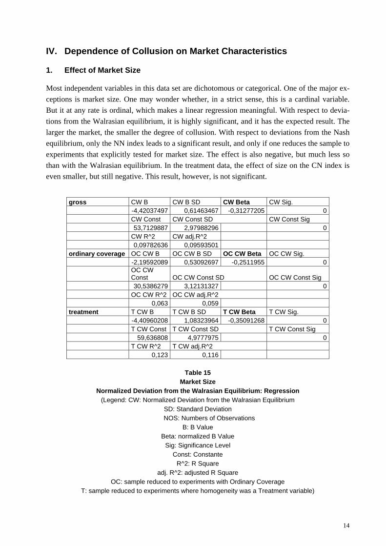
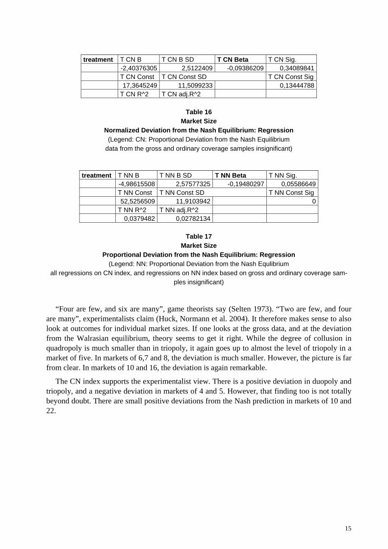
Most independent variables in this data set are dichotomous or categorical. One of the major ex-ceptions is market size. One may wonder whether, in a strict sense, this is a cardinal variable. But it at any rate is ordinal, which makes a linear regression meaningful. With respect to devia-tions from the Walrasian equilibrium, it is highly significant, and it has the expected result. The larger the market, the smaller the degree of collusion. With respect to deviations from the Nash equilibrium, only the NN index leads to a significant result, and only if one reduces the sample to experiments that explicitly tested for market size. The effect is also negative, but much less so than with the Walrasian equilibrium. In the treatment data, the effect of size on the CN index is even smaller, but still negative. This result, however, is not significant.

gross CW B CW B SD CW Beta CW Sig. -4,42037497 0,61463467 -0,31277205 0 CW Const CW Const SD CW Const Sig 53,7129887 2,97988296 0 CW R^2 CW adj.R^2 0,09782636 0,09593501 ordinary coverage OC CW B OC CW B SD OC CW Beta OC CW Sig. -2,19592089 0,53092697 -0,2511955 0

OC CW Const OC CW Const SD OC CW Const Sig

30,5386279 3,12131327 0 OC CW R^2 OC CW adj.R^2 0,063 0,059 treatment T CW B T CW B SD T CW Beta T CW Sig. -4,40960208 1,08323964 -0,35091268 0 T CW Const T CW Const SD T CW Const Sig 59,636808 4,9777975 0 T CW R^2 T CW adj.R^2 0,123 0,116

Table 15

Market Size Normalized Deviation from the Walrasian Equilibrium: Regression

(Legend: CW: Normalized Deviation from the Walrasian Equilibrium SD: Standard Deviation

NOS: Numbers of Observations B: B Value

Beta: normalized B Value Sig: Significance Level

Const: Constante R^2: R Square

adj. R^2: adjusted R Square OC: sample reduced to experiments with Ordinary Coverage

T: sample reduced to experiments where homogeneity was a Treatment variable)

15

treatment T CN B T CN B SD T CN Beta T CN Sig. -2,40376305 2,5122409 -0,09386209 0,34089841 T CN Const T CN Const SD T CN Const Sig 17,3645249 11,5099233 0,13444788 T CN R^2 T CN adj.R^2

Table 16

Market Size Normalized Deviation from the Nash Equilibrium: Regression

(Legend: CN: Proportional Deviation from the Nash Equilibrium data from the gross and ordinary coverage samples insignificant)

treatment T NN B T NN B SD T NN Beta T NN Sig. -4,98615508 2,57577325 -0,19480297 0,05586649 T NN Const T NN Const SD T NN Const Sig 52,5256509 11,9103942 0 T NN R^2 T NN adj.R^2 0,0379482 0,02782134

Table 17

Market Size Proportional Deviation from the Nash Equilibrium: Regression

(Legend: NN: Proportional Deviation from the Nash Equlibrium all regressions on CN index, and regressions on NN index based on gross and ordinary coverage sam-

ples insignificant)

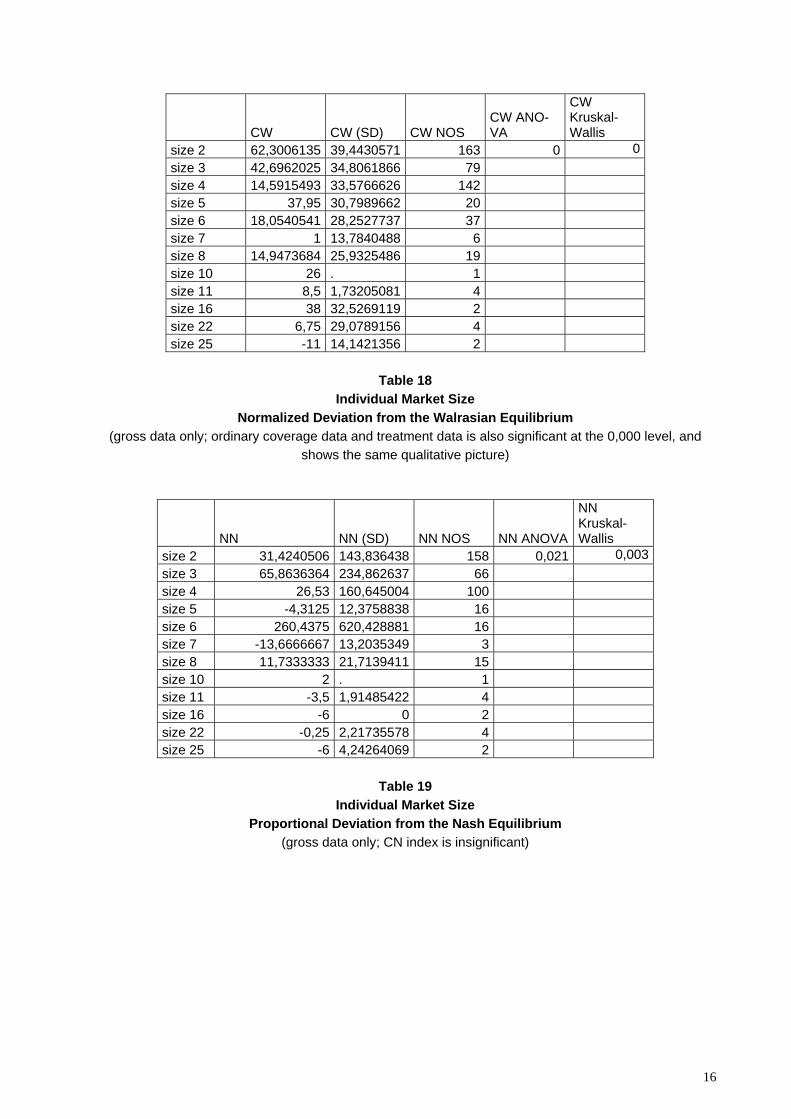
“Four are few, and six are many”, game theorists say (Selten 1973). “Two are few, and four are many”, experimentalists claim (Huck, Normann et al. 2004). It therefore makes sense to also look at outcomes for individual market sizes. If one looks at the gross data, and at the deviation from the Walrasian equilibrium, theory seems to get it right. While the degree of collusion in quadropoly is much smaller than in triopoly, it again goes up to almost the level of triopoly in a market of five. In markets of 6,7 and 8, the deviation is much smaller. However, the picture is far from clear. In markets of 10 and 16, the deviation is again remarkable.

The CN index supports the experimentalist view. There is a positive deviation in duopoly and triopoly, and a negative deviation in markets of 4 and 5. However, that finding too is not totally beyond doubt. There are small positive deviations from the Nash prediction in markets of 10 and 22.

16

CW CW (SD) CW NOS CW ANO-VA

CW Kruskal-Wallis

size 2 62,3006135 39,4430571 163 0 0 size 3 42,6962025 34,8061866 79 size 4 14,5915493 33,5766626 142 size 5 37,95 30,7989662 20 size 6 18,0540541 28,2527737 37 size 7 1 13,7840488 6 size 8 14,9473684 25,9325486 19 size 10 26 . 1 size 11 8,5 1,73205081 4 size 16 38 32,5269119 2 size 22 6,75 29,0789156 4 size 25 -11 14,1421356 2

Table 18

Individual Market Size Normalized Deviation from the Walrasian Equilibrium

(gross data only; ordinary coverage data and treatment data is also significant at the 0,000 level, and shows the same qualitative picture)

NN NN (SD) NN NOS NN ANOVA

NN Kruskal-Wallis

size 2 31,4240506 143,836438 158 0,021 0,003 size 3 65,8636364 234,862637 66 size 4 26,53 160,645004 100 size 5 -4,3125 12,3758838 16 size 6 260,4375 620,428881 16 size 7 -13,6666667 13,2035349 3 size 8 11,7333333 21,7139411 15 size 10 2 . 1 size 11 -3,5 1,91485422 4 size 16 -6 0 2 size 22 -0,25 2,21735578 4 size 25 -6 4,24264069 2

Table 19

Individual Market Size Proportional Deviation from the Nash Equilibrium

(gross data only; CN index is insignificant)

17

2. Symmetry vs. Asymmetry of Sellers

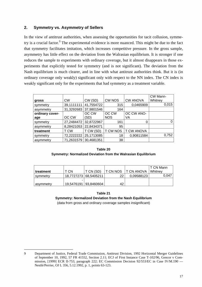
In the view of antitrust authorities, when assessing the opportunities for tacit collusion, symme-try is a crucial factor.9 The experimental evidence is more nuanced. This might be due to the fact that symmetry facilitates imitation, which increases competitive pressure. In the gross sample, asymmetry has little effect on the deviation from the Walrasian equilibrium. It is stronger if one reduces the sample to experiments with ordinary coverage, but it almost disappears in those ex-periments that explicitly tested for symmetry (and is not significant). The deviation from the Nash equilibrium is much clearer, and in line with what antitrust authorities think. But it is (in ordinary coverage only weakly) significant only with respect to the NN index. The CN index is weakly significant only for the experiments that had symmetry as a treatment variable.


symmetry 39,1111111 41,7554722 315 0,0465909 0,015asymmetry 31,3292683 37,9801546 164 ordinary cover-age OC CW

OC CW (SD)

OC CW NOS

OC CW ANO-VA

symmetry 27,2484472 32,8722967 161 0 0asymmetry 8,28421053 22,8434371 95 treatment T CW T CW (SD) T CW NOS T CW ANOVA symmetry 72,2222222 25,1713085 18 0,90811584 0,752asymmetry 71,2631579 30,4681351 38

Table 20

Symmetry: Normalized Deviation from the Walrasian Equilibrium


symmetry 18,7727273 68,5405211 22 0,09588123 0,047

asymmetry -

19,5476191 93,8460604 42

Table 21

Symmetry: Normalized Deviation from the Nash Equilibrium (data from gross and ordinary coverage samples insignificant)

9 Department of Justice, Federal Trade Commission, Antitrust Division, 1992 Horizontal Merger Guidelines

of September 10, 1992, 57 FR 41552, Section 2.11; ECJ of First Instance Case T-102/96, Gencor v Com-mission, [1999] ECR II-753, paragraph 222; EC Commission Decision 92/553/EC in Case IV/M.190 — Nestlé/Perrier, OJ L 356, 5.12.1992, p. 1, points 63-123.

18


symmetry 55,3498233 236,903865 283 0,03062506 0,026asymmetry 4,77884615 27,2756361 104 ordinary coverage OC NN OC NN (SD) OC NN NOS OC NN ANOVA symmetry 92,4592593 334,671632 135 0,06154268 0,002asymmetry -2,65909091 7,72173972 44 treatment T NN T NN (SD) T NN NOS T NN ANOVA symmetry 44,3888889 79,4859506 18 0,02969758 0,176asymmetry 8,81578947 40,2511408 38

Table 22

Symmetry: Proportional Deviation from the Nash Equilibrium Again, interaction effects help to understand the somewhat mixed evidence. It is particularly in-teresting to test for interactions with market size. Asymmetry increases collusion in markets of 2 and 3, but reduces it in larger markets. Moreover, symmetry hurts if gains from collusion are small, but it helps if there is a larger pie.

size size 2 size 2 (SD) size 2 NOS size Sig. symmetry 59,3082707 42,1597216 133 0,00060183asymmetry 75,5666667 19,4221405 30 size 3 size 3 (SD) size 3 NOS symmetry 33,4418605 29,2023338 43 asymmetry 53,75 38,0213286 36 size 4 size 4 (SD) size 4 NOS symmetry 18,626506 37,6708177 83 asymmetry 8,91525424 26,0452445 59 size 5 size 5 (SD) size 5 NOS symmetry 51 33,4932829 11 asymmetry 22 18,1727818 9 surplus producer surplus producer surplus (SD) producer surplus NOS surplus Sig.symmetry -18,375 38,9539563 8 0,00137745asymmetry 25,1176471 30,7284118 17 symmetric surplus symmetric surplus (SD) symmetric surplus NOS symmetry 27,6981132 33,1364193 106 asymmetry 3,34615385 17,7153996 26 consumer surplus consumer surplus (SD) consumer surplus NOS symmetry 48,5103093 43,0939737 194 asymmetry 38,214876 39,3086518 121

Table 23

Symmetry: Interaction Effects (normalized deviation from the Walrasian equilibrium)

19

3. fect of Power Asymmetries among Sellers

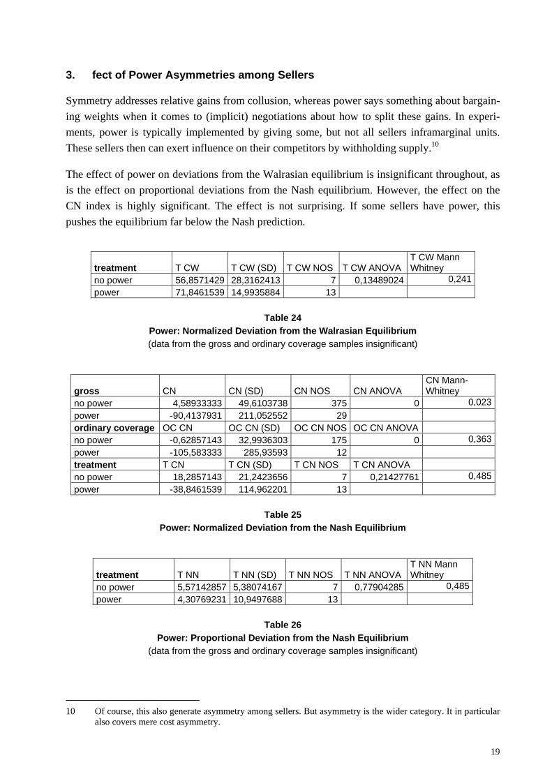
Symmetry addresses relative gains from collusion, whereas power says something about bargain-ing weights when it comes to (implicit) negotiations about how to split these gains. In experi-ments, power is typically implemented by giving some, but not all sellers inframarginal units. These sellers then can exert influence on their competitors by withholding supply.10

The effect of power on deviations from the Walrasian equilibrium is insignificant throughout, as is the effect on proportional deviations from the Nash equilibrium. However, the effect on the CN index is highly significant. The effect is not surprising. If some sellers have power, this pushes the equilibrium far below the Nash prediction.

treatment T CW T CW (SD) T CW NOS T CW ANOVA T CW Mann Whitney

no power 56,8571429 28,3162413 7 0,13489024 0,241power 71,8461539 14,9935884 13

Table 24

Power: Normalized Deviation from the Walrasian Equilibrium (data from the gross and ordinary coverage samples insignificant)


no power 4,58933333 49,6103738 375 0 0,023power -90,4137931 211,052552 29 ordinary coverage OC CN OC CN (SD) OC CN NOS OC CN ANOVA no power -0,62857143 32,9936303 175 0 0,363power -105,583333 285,93593 12 treatment T CN T CN (SD) T CN NOS T CN ANOVA no power 18,2857143 21,2423656 7 0,21427761 0,485power -38,8461539 114,962201 13

Table 25

Power: Normalized Deviation from the Nash Equilibrium


no power 5,57142857 5,38074167 7 0,77904285 0,485power 4,30769231 10,9497688 13

Table 26

Power: Proportional Deviation from the Nash Equilibrium (data from the gross and ordinary coverage samples insignificant)

10 Of course, this also generate asymmetry among sellers. But asymmetry is the wider category. It in particular

also covers mere cost asymmetry.

20

V. Dependence of Collusion on Demand and Supply Characteristics

1. Effect of Demand Characteristics

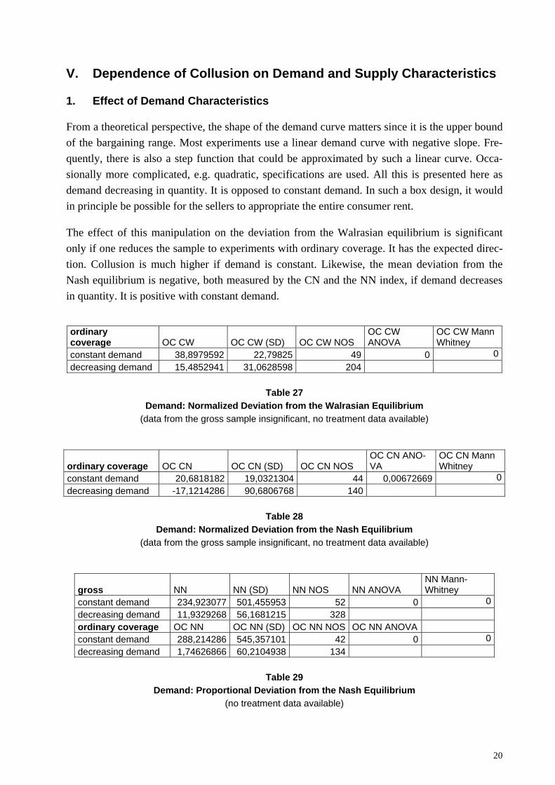
From a theoretical perspective, the shape of the demand curve matters since it is the upper bound of the bargaining range. Most experiments use a linear demand curve with negative slope. Fre-quently, there is also a step function that could be approximated by such a linear curve. Occa-sionally more complicated, e.g. quadratic, specifications are used. All this is presented here as demand decreasing in quantity. It is opposed to constant demand. In such a box design, it would in principle be possible for the sellers to appropriate the entire consumer rent.

The effect of this manipulation on the deviation from the Walrasian equilibrium is significant only if one reduces the sample to experiments with ordinary coverage. It has the expected direc-tion. Collusion is much higher if demand is constant. Likewise, the mean deviation from the Nash equilibrium is negative, both measured by the CN and the NN index, if demand decreases in quantity. It is positive with constant demand.

ordinary coverage OC CW OC CW (SD) OC CW NOS

OC CW ANOVA

OC CW Mann Whitney

constant demand 38,8979592 22,79825 49 0 0decreasing demand 15,4852941 31,0628598 204

Table 27

Demand: Normalized Deviation from the Walrasian Equilibrium (data from the gross sample insignificant, no treatment data available)

ordinary coverage OC CN OC CN (SD) OC CN NOS OC CN ANO-VA

OC CN Mann Whitney

constant demand 20,6818182 19,0321304 44 0,00672669 0decreasing demand -17,1214286 90,6806768 140

Table 28

Demand: Normalized Deviation from the Nash Equilibrium (data from the gross sample insignificant, no treatment data available)


constant demand 234,923077 501,455953 52 0 0decreasing demand 11,9329268 56,1681215 328 ordinary coverage OC NN OC NN (SD) OC NN NOS OC NN ANOVA constant demand 288,214286 545,357101 42 0 0decreasing demand 1,74626866 60,2104938 134

Table 29

Demand: Proportional Deviation from the Nash Equilibrium (no treatment data available)

21

2. Effect of Supply Characteristics

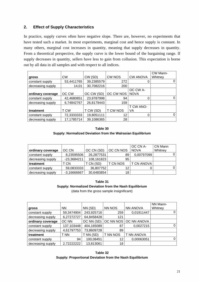
In practice, supply curves often have negative slope. There are, however, no experiments that have tested such a market. In most experiments, marginal cost and hence supply is constant. In many others, marginal cost increases in quantity, meaning that supply decreases in quantity. From a theoretical perspective, the supply curve is the lower bound of the bargaining range. If supply decreases in quantity, sellers have less to gain from collusion. This expectation is borne out by all data in all samples and with respect to all indices.


constant supply 53,4411765 39,2385579 272 0 0decreasing supply 14,01 30,7082216 200

ordinary coverage OC CW OC CW (SD) OC CW NOSOC CW A-NOVA


treatment T CW T CW (SD) T CW NOS T CW ANO-VA


Table 30

Supply: Normalized Deviation from the Walrasian Equilibrium

ordinary coverage OC CN OC CN (SD) OC CN NOS OC CN A-NOVA

CN Mann Whitney

constant supply 8,23595506 26,2877531 89 0,00797099 0decreasing supply -23,3684211 108,161823 95 treatment T CN T CN (SD) T CN NOS T CN ANOVA constant supply 59,0833333 36,807752 12 0 0decreasing supply -3,16666667 30,6483854 18

Table 31

Supply: Normalized Deviation from the Nash Equilibrium (data from the gross sample insignificant)


constant supply 59,3474904 243,925716 259 0,01911447 0decreasing supply 6,27272727 64,8458428 121 ordinary coverage OC NN OC NN (SD) OC NN NOS OC NN ANOVA constant supply 137,103448 404,165089 87 0,0027215 0decreasing supply 4,61797753 73,8609728 89 treatment T NN T NN (SD) T NN NOS T NN ANOVA constant supply 94 100,08451 12 0,00063051 0decreasing supply 2,72222222 13,813061 18

Table 32

Supply: Proportional Deviation from the Nash Equilibrium

22

3. Dependence of Collusion on the Distribution of the Surplus

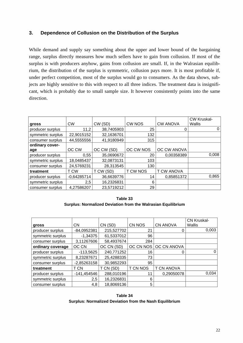
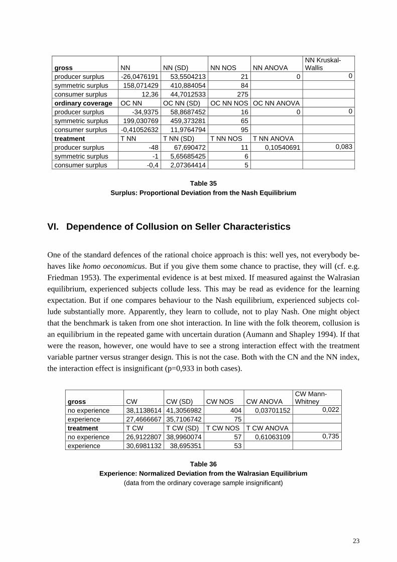
While demand and supply say something about the upper and lower bound of the bargaining range, surplus directly measures how much sellers have to gain from collusion. If most of the surplus is with producers anyhow, gains from collusion are small. If, in the Walrasian equilib-rium, the distribution of the surplus is symmetric, collusion pays more. It is most profitable if, under perfect competition, most of the surplus would go to consumers. As the data shows, sub-jects are highly sensitive to this with respect to all three indices. The treatment data is insignifi-cant, which is probably due to small sample size. It however consistently points into the same direction.

gross CW CW (SD) CW NOS CW ANOVA CW Kruskal-Wallis

producer surplus 11,2 38,7405903 25 0 0symmetric surplus 22,9015152 32,1636701 132 consumer surplus 44,5555556 41,9180949 315 ordinary cover-age OC CW OC CW (SD) OC CW NOS OC CW ANOVA

producer surplus 0,55 35,0690672 20 0,00358389 0,008symmetric surplus 18,0485437 32,0873131 103 consumer surplus 24,5769231 28,313545 130 treatment T CW T CW (SD) T CW NOS T CW ANOVA producer surplus -0,64285714 36,6639776 14 0,85851372 0,865symmetric surplus 2,5 16,2326831 6 consumer surplus 4,27586207 23,5719212 29

Table 33 Surplus: Normalized Deviation from the Walrasian Equilibrium

gross CN CN (SD) CN NOS CN ANOVA CN Kruskal-Wallis

producer surplus -84,0952381 215,527702 21 0 0,003symmetric surplus -1,34375 61,5337012 96 consumer surplus 3,11267606 58,4937674 284 ordinary coverage OC CN OC CN (SD) OC CN NOS OC CN ANOVA producer surplus -113,5625 240,771252 16 0 0symmetric surplus 8,23287671 25,4288335 73 consumer surplus -2,85263158 30,9852293 95 treatment T CN T CN (SD) T CN NOS T CN ANOVA producer surplus -141,454546 288,010196 11 0,29050078 0,034symmetric surplus 2,5 16,2326831 6 consumer surplus 4,8 18,8069136 5

Table 34

Surplus: Normalized Deviation from the Nash Equilibrium

23

gross NN NN (SD) NN NOS NN ANOVA NN Kruskal-Wallis

producer surplus -26,0476191 53,5504213 21 0 0symmetric surplus 158,071429 410,884054 84 consumer surplus 12,36 44,7012533 275 ordinary coverage OC NN OC NN (SD) OC NN NOS OC NN ANOVA producer surplus -34,9375 58,8687452 16 0 0symmetric surplus 199,030769 459,373281 65 consumer surplus -0,41052632 11,9764794 95 treatment T NN T NN (SD) T NN NOS T NN ANOVA producer surplus -48 67,690472 11 0,10540691 0,083symmetric surplus -1 5,65685425 6 consumer surplus -0,4 2,07364414 5

Table 35

Surplus: Proportional Deviation from the Nash Equilibrium

VI. Dependence of Collusion on Seller Characteristics

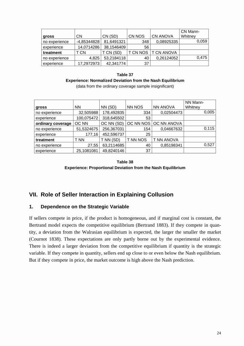
One of the standard defences of the rational choice approach is this: well yes, not everybody be-haves like homo oeconomicus. But if you give them some chance to practise, they will (cf. e.g. Friedman 1953). The experimental evidence is at best mixed. If measured against the Walrasian equilibrium, experienced subjects collude less. This may be read as evidence for the learning expectation. But if one compares behaviour to the Nash equilibrium, experienced subjects col-lude substantially more. Apparently, they learn to collude, not to play Nash. One might object that the benchmark is taken from one shot interaction. In line with the folk theorem, collusion is an equilibrium in the repeated game with uncertain duration (Aumann and Shapley 1994). If that were the reason, however, one would have to see a strong interaction effect with the treatment variable partner versus stranger design. This is not the case. Both with the CN and the NN index, the interaction effect is insignificant (p=0,933 in both cases).


no experience 38,1138614 41,3056982 404 0,03701152 0,022experience 27,4666667 35,7106742 75 treatment T CW T CW (SD) T CW NOS T CW ANOVA no experience 26,9122807 38,9960074 57 0,61063109 0,735experience 30,6981132 38,695351 53

Table 36

Experience: Normalized Deviation from the Walrasian Equilibrium (data from the ordinary coverage sample insignificant)

24


no experience -4,85344828 81,6491321 348 0,08925335 0,059experience 14,0714286 38,1546409 56 treatment T CN T CN (SD) T CN NOS T CN ANOVA no experience 4,825 53,2184118 40 0,26124052 0,475experience 17,2972973 42,341774 37

Table 37

Experience: Normalized Deviation from the Nash Equilibrium (data from the ordinary coverage sample insignificant)


no experience 32,505988 178,492835 334 0,02504473 0,005experience 100,075472 318,645502 53 ordinary coverage OC NN OC NN (SD) OC NN NOS OC NN ANOVA no experience 51,5324675 256,367031 154 0,04667632 0,115experience 177,16 452,596737 25 treatment T NN T NN (SD) T NN NOS T NN ANOVA no experience 27,55 63,2114685 40 0,85198341 0,527experience 25,1081081 49,8240146 37

Table 38

Experience: Proportional Deviation from the Nash Equilibrium

VII. Role of Seller Interaction in Explaining Collusion

1. Dependence on the Strategic Variable

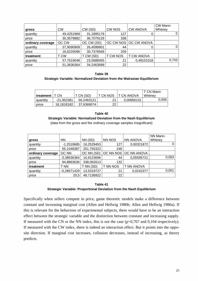
If sellers compete in price, if the product is homogeneous, and if marginal cost is constant, the Bertrand model expects the competitive equilibrium (Bertrand 1883). If they compete in quan-tity, a deviation from the Walrasian equilibrium is expected, the larger the smaller the market (Cournot 1838). These expectations are only partly borne out by the experimental evidence. There is indeed a larger deviation from the competitive equilibrium if quantity is the strategic variable. If they compete in quantity, sellers end up close to or even below the Nash equilibrium. But if they compete in price, the market outcome is high above the Nash prediction.

25


quantity 49,4251969 31,1895179 127 0 0price 30,3579882 36,7079129 338 ordinary coverage OC CW OC CW (SD) OC CW NOS OC CW ANOVA quantity 37,9090909 26,4599901 44 0 0price 16,6220096 30,7376569 209 treatment T CW T CW (SD) T CW NOS T CW ANOVA quantity 57,7619048 23,5688455 21 0,48151018 0,743price 51,3636364 34,2463699 22

Table 39

Strategic Variable: Normalized Deviation from the Walrasian Equilibrium


quantity -21,952381 56,2463121 21 0,00856131 0,006price 18,1818182 37,6369074 22

Table 40

Strategic Variable: Normalized Deviation from the Nash Equilibrium (data from the gross and the ordinary coverage samples insignificant)


quantity -1,2519685 16,2529453 127 0,00321872 0price 65,1048387 251,755322 248 ordinary coverage OC NN OC NN (SD) OC NN NOS OC NN ANOVA quantity -3,38636364 10,9123696 44 0,05595721 0,003price 94,8863636 338,062613 132 treatment T NN T NN (SD) T NN NOS T NN ANOVA quantity -5,28571429 13,5319727 21 0,0242377 0,001price 20,5 48,7136922 22

Table 41

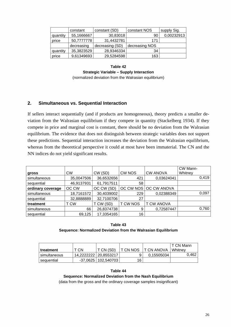
Strategic Variable: Proportional Deviation from the Nash Equilibrium Specifically when sellers compete in price, game theoretic models make a difference between constant and increasing marginal cost (Allen and Hellwig 1986b; Allen and Hellwig 1986a). If this is relevant for the behaviour of experimental subjects, there would have to be an interaction effect between the strategic variable and the distinction between constant and increasing supply. If measured with the CN or the NN index, this is not the case (p=0,767 and 0,104 respectively). If measured with the CW index, there is indeed an interaction effect. But it points into the oppo-site direction. If marginal cost increases, collusion decreases, instead of increasing, as theory predicts.

26

constant constant (SD) constant NOS supply Sig. quantity 55,1666667 30,83018 90 0,00232913 price 50,7777778 31,4432781 171 decreasing decreasing (SD) decreasing NOS quantity 35,3823529 28,9346334 34 price 9,61349693 29,5284598 163

Table 42

Strategic Variable – Supply Interaction (normalized deviation from the Walrasian equilibrium)

2. Simultaneous vs. Sequential Interaction

If sellers interact sequentially (and if products are homogeneous), theory predicts a smaller de-viation from the Walrasian equilibrium if they compete in quantity (Stackelberg 1934). If they compete in price and marginal cost is constant, there should be no deviation from the Walrasian equilibrium. The evidence that does not distinguish between strategic variables does not support these predictions. Sequential interaction increases the deviation from the Walrasian equilibrium, whereas from the theoretical perspective it could at most have been immaterial. The CN and the NN indices do not yield significant results.


simultaneous 35,0047506 36,6532656 421 0,03624041 0,419sequential 46,9137931 61,7917511 58 ordinary coverage OC CW OC CW (SD) OC CW NOS OC CW ANOVA simultaneous 18,7161572 30,4039002 229 0,02388349 0,097sequential 32,8888889 32,7100706 27 treatment T CW T CW (SD) T CW NOS T CW ANOVA simultaneous 66 26,8374738 9 0,72587447 0,760sequential 69,125 17,3354165 16

Table 43 Sequence: Normalized Deviation from the Walrasian Equilibrium


simultaneous 14,2222222 20,8553217 9 0,15505034 0,462sequential -37,0625 102,540703 16

Table 44

Sequence: Normalized Deviation from the Nash Equilibrium (data from the gross and the ordinary coverage samples insignificant)

27

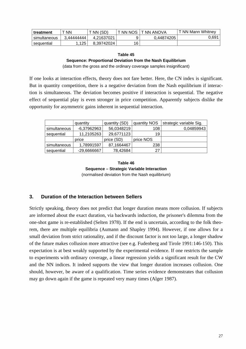
treatment T NN T NN (SD) T NN NOS T NN ANOVA T NN Mann Whitney simultaneous 3,44444444 4,21637021 9 0,44874205 0,691sequential 1,125 8,39742024 16

Table 45

Sequence: Proportional Deviation from the Nash Equilibrium (data from the gross and the ordinary coverage samples insignificant)

If one looks at interaction effects, theory does not fare better. Here, the CN index is significant. But in quantity competition, there is a negative deviation from the Nash equilibrium if interac-tion is simultaneous. The deviation becomes positive if interaction is sequential. The negative effect of sequential play is even stronger in price competition. Apparently subjects dislike the opportunity for asymmetric gains inherent in sequential interaction.

quantity quantity (SD) quantity NOS strategic variable Sig. simultaneous -6,37962963 56,0348219 108 0,04859943sequential 11,2105263 29,6771123 19 price price (SD) price NOS simultaneous 1,78991597 87,1664467 238 sequential -29,6666667 78,42684 27

Table 46 Sequence – Strategic Variable Interaction

(normalised deviation from the Nash equilibrium)

3. Duration of the Interaction between Sellers

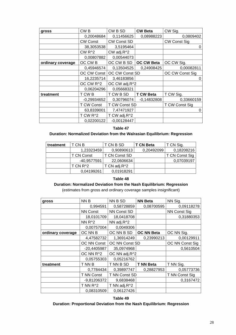
Strictly speaking, theory does not predict that longer duration means more collusion. If subjects are informed about the exact duration, via backwards induction, the prisoner's dilemma from the one-shot game is re-established (Selten 1978). If the end is uncertain, according to the folk theo-rem, there are multiple equilibria (Aumann and Shapley 1994). However, if one allows for a small deviation from strict rationality, and if the discount factor is not too large, a longer shadow of the future makes collusion more attractive (see e.g. Fudenberg and Tirole 1991:146-150). This expectation is at best weakly supported by the experimental evidence. If one restricts the sample to experiments with ordinary coverage, a linear regression yields a significant result for the CW and the NN indices. It indeed supports the view that longer duration increases collusion. One should, however, be aware of a qualification. Time series evidence demonstrates that collusion may go down again if the game is repeated very many times (Alger 1987).

28

gross CW B CW B SD CW Beta CW Sig. 0,20048684 0,11456625 0,08988223 0,0809402 CW Const CW Const SD CW Const Sig 38,3053538 3,5195464 0 CW R^2 CW adj.R^2 0,00807882 0,00544073 ordinary coverage OC CW B OC CW B SD OC CW Beta OC CW Sig. 0,45946574 0,13504525 0,24908425 0,00082811 OC CW Const OC CW Const SD OC CW Const Sig 16,2235714 3,46183856 0 OC CW R^2 OC CW adj.R^2 0,06204296 0,05668321 treatment T CW B T CW B SD T CW Beta T CW Sig. -0,29934652 0,30796074 -0,14832808 0,33660159 T CW Const T CW Const SD T CW Const Sig 63,8339001 7,47471927 0 T CW R^2 T CW adj.R^2 0,02200122 -0,00128447

Table 47 Duration: Normalized Deviation from the Walrasian Equilibrium: Regression

treatment T CN B T CN B SD T CN Beta T CN Sig. 1,23323459 0,90890613 0,20492099 0,18208216 T CN Const T CN Const SD T CN Const Sig -40,9577591 22,0606634 0,07039197 T CN R^2 T CN adj.R^2 0,04199261 0,01918291

Table 48 Duration: Normalized Deviation from the Nash Equilibrium: Regression

(estimates from gross and ordinary coverage samples insignificant)

gross NN B NN B SD NN Beta NN Sig. 0,994591 0,58728859 0,08700595 0,09118278 NN Const NN Const SD NN Const Sig 18,0101709 18,0418708 0,31880353 NN R^2 NN adj.R^2 0,00757004 0,0049306 ordinary coverage OC NN B OC NN B SD OC NN Beta OC NN Sig. 4,47582732 1,36914249 0,23990213 0,00129911 OC NN Const OC NN Const SD OC NN Const Sig -20,4405987 35,0974968 0,5610504 OC NN R^2 OC NN adj.R^2 0,05755303 0,05216762 treatment T NN B T NN B SD T NN Beta T NN Sig. 0,7784434 0,39897747 0,28827953 0,05773736 T NN Const T NN Const SD T NN Const Sig -9,81206372 9,6838468 0,3167472 T NN R^2 T NN adj.R^2 0,08310509 0,06127426

Table 49 Duration: Proportional Deviation from the Nash Equilibrium: Regression

29

4. Partner vs. Stranger Design

It is more interesting, and more relevant, to compare experiments that had a fixed partner design with others that rematched subjects from round to round. On average, the latter manipulation increases collusion with respect to all three indices.


partner 34,5250597 42,0143085 419 0,006 0,001stranger 49,8666667 25,682195 60 ordinary coverage OC CW OC CW (SD) OC CW NOS OC CW ANOVA partner 16,7882883 30,6395664 222 0 0stranger 42,5588235 22,2794799 34 treatment T CW T CW (SD) T CW NOS T CW ANOVA partner 61,8421053 21,5748391 19 0,853 0,811stranger 60,5 23,2797631 20

Table 50 Partner vs. Stranger Design

Normalized Deviation from the Walrasian Equilibrium

ordinary coverage OC CN OC CN (SD) OC CN NOS OC CN ANOVA CN Mann Whit-ney

partner -11,8846154 87,1616194 156 0,086 0stranger 15,3870968 22,8599758 31 treatment T CN T CN (SD) T CN NOS T CN ANOVA partner -8,89473684 70,2178315 19 0,656 0,440stranger -20,05 84,0829634 20

Table 51

Partner vs. Stranger Design Normalized Deviation from the Nash Equilibrium

(gross data insignificant)


partner 24,0684524 151,842804 336 0 0stranger 158,313725 389,258448 51 ordinary coverage OC NN OC NN (SD) OC NN NOS OC NN ANOVA partner 30,5666667 219,584581 150 0 0stranger 268,275862 491,13243 29 treatment T NN T NN (SD) T NN NOS T NN ANOVA partner 13,2631579 42,6872894 19 0,523 0,704stranger 6,35 21,4089873 20

Table 52 Partner vs. Stranger Design

Proportional Deviation from the Nash Equilibrium

These are surprising findings, both compared to the theoretical prediction, and to the findings in those experiments that had the distinction between partner and stranger design as a treatment variable. From the already mentioned folk theorem it follows that theory makes no clear predic-

30

tion for the repeated game (Aumann and Shapley 1994). But one result is beyond doubt. In one-shot interaction, there is no collusive equilibrium. (Bertrand 1883) and (Cournot 1838) agree on this. It is equally remarkable that in the subsample with experiments that explicitly tested for the effect, the distinction between the partner and the stranger design is insignificant for all three indices.

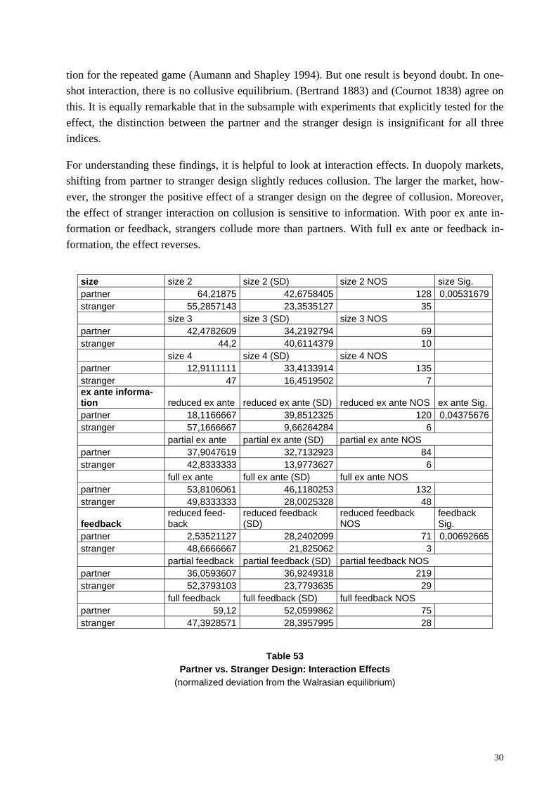
For understanding these findings, it is helpful to look at interaction effects. In duopoly markets, shifting from partner to stranger design slightly reduces collusion. The larger the market, how-ever, the stronger the positive effect of a stranger design on the degree of collusion. Moreover, the effect of stranger interaction on collusion is sensitive to information. With poor ex ante in-formation or feedback, strangers collude more than partners. With full ex ante or feedback in-formation, the effect reverses.

size size 2 size 2 (SD) size 2 NOS size Sig. partner 64,21875 42,6758405 128 0,00531679stranger 55,2857143 23,3535127 35 size 3 size 3 (SD) size 3 NOS partner 42,4782609 34,2192794 69 stranger 44,2 40,6114379 10 size 4 size 4 (SD) size 4 NOS partner 12,9111111 33,4133914 135 stranger 47 16,4519502 7 ex ante informa-tion reduced ex ante reduced ex ante (SD) reduced ex ante NOS ex ante Sig.partner 18,1166667 39,8512325 120 0,04375676stranger 57,1666667 9,66264284 6 partial ex ante partial ex ante (SD) partial ex ante NOS partner 37,9047619 32,7132923 84 stranger 42,8333333 13,9773627 6 full ex ante full ex ante (SD) full ex ante NOS partner 53,8106061 46,1180253 132 stranger 49,8333333 28,0025328 48

feedback reduced feed-back

reduced feedback (SD)

reduced feedback NOS

feedback Sig.

partner 2,53521127 28,2402099 71 0,00692665stranger 48,6666667 21,825062 3 partial feedback partial feedback (SD) partial feedback NOS partner 36,0593607 36,9249318 219 stranger 52,3793103 23,7793635 29 full feedback full feedback (SD) full feedback NOS partner 59,12 52,0599862 75 stranger 47,3928571 28,3957995 28

Table 53 Partner vs. Stranger Design: Interaction Effects

(normalized deviation from the Walrasian equilibrium)

31

This explanation is corroborated if one checks the distribution of market sizes in the subsample that has explicitly tested the stranger versus the partner design. 33 experiments had a duopoly market, 6 a quadropoly. 27 had full, 12 partial ex ante information, none reduced information. 18 had full and 18 partial, and only 3 reduced feedback. In the subsample, treatment variables are thus overrepresented that dampen the effect of a stranger design on collusion.

5. Effect of Communication on Collusion

In game theoretic terms, competition puts sellers into a prisoner's dilemma.11 If they have a chance to talk before play, from a theoretical perspective this is just irrelevant “cheap talk“ (for background and alternative models see Crawford 1998). Indeed, the main effect is not significant with respect to the CW and the NN indices. Only the CN index shows what common sense would expect: communication increases collusion.

treatment T CW T CW (SD) T CW NOS T CW ANOVA T CW Mann Whitney

no communication 47,5555556 125,966376 9 0,80658175 0,042communication 57,6153846 63,1948554 13

Table 54

Communication: Normalized Deviation from the Walrasian Equilibrium (data from gross and ordinary coverage samples insignificant)


no communication -4,99171271 80,3984705 362 0,0349576 0,006communication 21,5714286 35,1374603 42 treatment T CN T CN (SD) T CN NOS T CN ANOVA no communication 3,11111111 21,1509128 9 0,003486 0,003communication 45 33,4713808 13

Table 55

Communication: Normalized Deviation from the Nash Equilibrium (data from ordinary coverage sample insignificant)


no communication 29,875 65,9641407 8 0,19233194 0,051communication 116,9 170,040159 10

Table 56

Communication: Proportional Deviation from the Nash Equilibrium (data from gross and ordinary coverage samples insignificant)

11 Strictly speaking, this only holds if marginal cost increases. But if the supply curve differs from this, the

parties still face a dilemma.

32

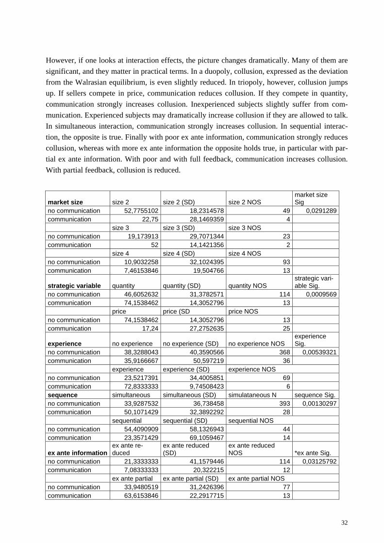
However, if one looks at interaction effects, the picture changes dramatically. Many of them are significant, and they matter in practical terms. In a duopoly, collusion, expressed as the deviation from the Walrasian equilibrium, is even slightly reduced. In triopoly, however, collusion jumps up. If sellers compete in price, communication reduces collusion. If they compete in quantity, communication strongly increases collusion. Inexperienced subjects slightly suffer from com-munication. Experienced subjects may dramatically increase collusion if they are allowed to talk. In simultaneous interaction, communication strongly increases collusion. In sequential interac-tion, the opposite is true. Finally with poor ex ante information, communication strongly reduces collusion, whereas with more ex ante information the opposite holds true, in particular with par-tial ex ante information. With poor and with full feedback, communication increases collusion. With partial feedback, collusion is reduced.

market size size 2 size 2 (SD) size 2 NOS market size Sig

no communication 52,7755102 18,2314578 49 0,0291289communication 22,75 28,1469359 4 size 3 size 3 (SD) size 3 NOS no communication 19,173913 29,7071344 23 communication 52 14,1421356 2 size 4 size 4 (SD) size 4 NOS no communication 10,9032258 32,1024395 93 communication 7,46153846 19,504766 13

strategic variable quantity quantity (SD) quantity NOS strategic vari-able Sig.

no communication 46,6052632 31,3782571 114 0,0009569communication 74,1538462 14,3052796 13 price price (SD price NOS no communication 74,1538462 14,3052796 13 communication 17,24 27,2752635 25

experience no experience no experience (SD) no experience NOS experience Sig.

no communication 38,3288043 40,3590566 368 0,00539321communication 35,9166667 50,597219 36 experience experience (SD) experience NOS no communication 23,5217391 34,4005851 69 communication 72,8333333 9,74508423 6 sequence simultaneous simultaneous (SD) simulataneous N sequence Sig.no communication 33,9287532 36,738458 393 0,00130297communication 50,1071429 32,3892292 28 sequential sequential (SD) sequential NOS no communication 54,4090909 58,1326943 44 communication 23,3571429 69,1059467 14

ex ante information ex ante re-duced

ex ante reduced (SD)

ex ante reduced NOS *ex ante Sig.

no communication 21,3333333 41,1579446 114 0,03125792communication 7,08333333 20,322215 12 ex ante partial ex ante partial (SD) ex ante partial NOS no communication 33,9480519 31,2426396 77 communication 63,6153846 22,2917715 13

33

ex ante full ex ante full (SD) ex ante full NOS no communication 52,1197605 39,6774347 167 communication 60,8461538 66,9450598 13 feedback informa-tion

reduced feed-back


reduced feedback NOS *feedback Sig.

no communication 4,15942029 29,7744577 69 0,0173197communication 7,8 25,2922913 5 partial feedback partial feedback (SD) partial feedback NOS no communication 39,650655 36,1609494 229 communication 17,6842105 27,166263 19 full feedback full feedback (SD) full feedback NOS no communication 53,9354839 43,9032549 93 communication 74,5 69,9082732 10

Table 57 Communication: Interaction Effects


6. Option to Agree

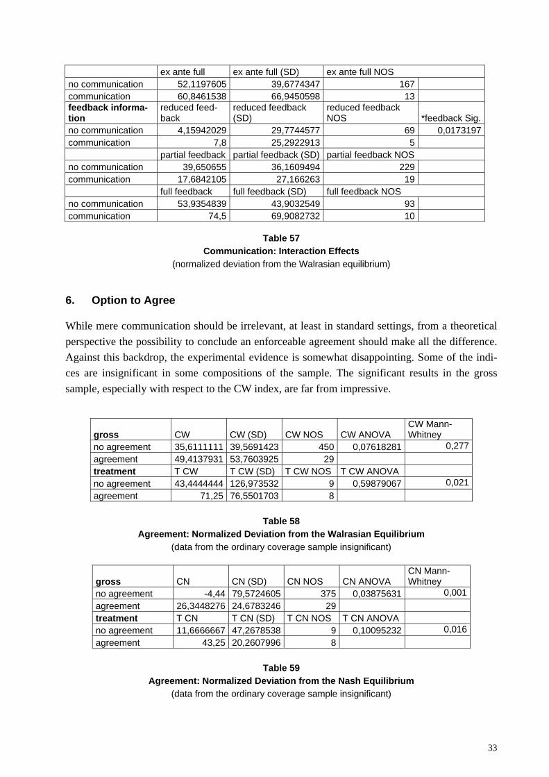
While mere communication should be irrelevant, at least in standard settings, from a theoretical perspective the possibility to conclude an enforceable agreement should make all the difference. Against this backdrop, the experimental evidence is somewhat disappointing. Some of the indi-ces are insignificant in some compositions of the sample. The significant results in the gross sample, especially with respect to the CW index, are far from impressive.


no agreement 35,6111111 39,5691423 450 0,07618281 0,277agreement 49,4137931 53,7603925 29 treatment T CW T CW (SD) T CW NOS T CW ANOVA no agreement 43,4444444 126,973532 9 0,59879067 0,021agreement 71,25 76,5501703 8

Table 58

Agreement: Normalized Deviation from the Walrasian Equilibrium (data from the ordinary coverage sample insignificant)


no agreement -4,44 79,5724605 375 0,03875631 0,001agreement 26,3448276 24,6783246 29 treatment T CN T CN (SD) T CN NOS T CN ANOVA no agreement 11,6666667 47,2678538 9 0,10095232 0,016agreement 43,25 20,2607996 8

Table 59

Agreement: Normalized Deviation from the Nash Equilibrium (data from the ordinary coverage sample insignificant)

34


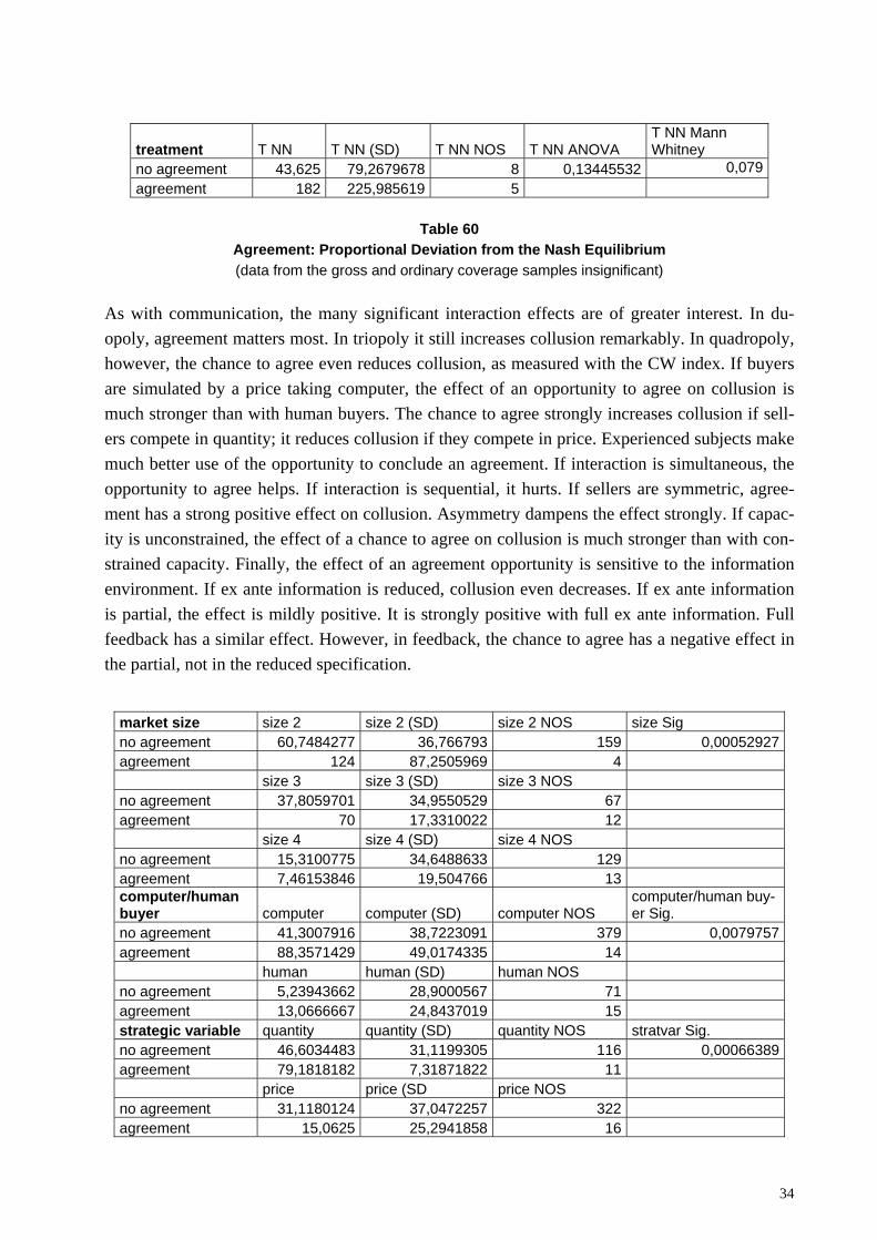
no agreement 43,625 79,2679678 8 0,13445532 0,079agreement 182 225,985619 5

Table 60

Agreement: Proportional Deviation from the Nash Equilibrium (data from the gross and ordinary coverage samples insignificant)

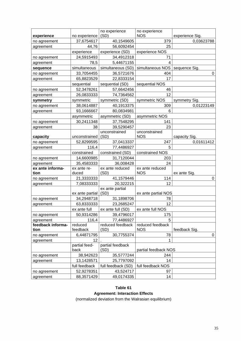
As with communication, the many significant interaction effects are of greater interest. In du-opoly, agreement matters most. In triopoly it still increases collusion remarkably. In quadropoly, however, the chance to agree even reduces collusion, as measured with the CW index. If buyers are simulated by a price taking computer, the effect of an opportunity to agree on collusion is much stronger than with human buyers. The chance to agree strongly increases collusion if sell-ers compete in quantity; it reduces collusion if they compete in price. Experienced subjects make much better use of the opportunity to conclude an agreement. If interaction is simultaneous, the opportunity to agree helps. If interaction is sequential, it hurts. If sellers are symmetric, agree-ment has a strong positive effect on collusion. Asymmetry dampens the effect strongly. If capac-ity is unconstrained, the effect of a chance to agree on collusion is much stronger than with con-strained capacity. Finally, the effect of an agreement opportunity is sensitive to the information environment. If ex ante information is reduced, collusion even decreases. If ex ante information is partial, the effect is mildly positive. It is strongly positive with full ex ante information. Full feedback has a similar effect. However, in feedback, the chance to agree has a negative effect in the partial, not in the reduced specification.

market size size 2 size 2 (SD) size 2 NOS size Sig no agreement 60,7484277 36,766793 159 0,00052927agreement 124 87,2505969 4 size 3 size 3 (SD) size 3 NOS no agreement 37,8059701 34,9550529 67 agreement 70 17,3310022 12 size 4 size 4 (SD) size 4 NOS no agreement 15,3100775 34,6488633 129 agreement 7,46153846 19,504766 13 computer/human buyer computer computer (SD) computer NOS

computer/human buy-er Sig.

no agreement 41,3007916 38,7223091 379 0,0079757agreement 88,3571429 49,0174335 14 human human (SD) human NOS no agreement 5,23943662 28,9000567 71 agreement 13,0666667 24,8437019 15 strategic variable quantity quantity (SD) quantity NOS stratvar Sig. no agreement 46,6034483 31,1199305 116 0,00066389agreement 79,1818182 7,31871822 11 price price (SD price NOS no agreement 31,1180124 37,0472257 322 agreement 15,0625 25,2941858 16

35

experience no experience no experience (SD)

no experience NOS experience Sig.

no agreement 37,6754617 40,1549605 379 0,03623788agreement 44,76 56,6092454 25 experience experience (SD) experience NOS no agreement 24,5915493 34,4912318 71 agreement 78,5 5,44671155 4 sequence simultaneous simultaneous (SD) simultaneous NOS sequence Sig. no agreement 33,7054455 36,5721676 404 0agreement 65,8823529 22,8333154 17 sequential sequential (SD) sequential NOS no agreement 52,3478261 57,6642456 46 agreement 26,0833333 74,7364562 12 symmetry symmetric symmetric (SD) symmetric NOS symmetry Sig. no agreement 38,0614887 40,1913375 309 0,01223149agreement 93,1666667 80,0834981 6 asymmetric asymmetric (SD) asymmetric NOS no agreement 30,2411348 37,7548295 141 agreement 38 39,5290457 23

capacity unconstrained unconstrained (SD)

unconstrained NOS capacity Sig.

no agreement 52,8299595 37,0413337 247 0,01611412agreement 116,4 77,4486927 5 constrained constrained (SD) constrained NOS no agreement 14,6600985 31,7120044 203 agreement 35,4583333 36,008428 24 ex ante informa-tion

ex ante re-duced

ex ante reduced (SD)

ex ante reduced NOS ex ante Sig.

no agreement 21,3333333 41,1579446 114 0agreement 7,08333333 20,322215 12

ex ante partial ex ante partial (SD) ex ante partial NOS

no agreement 34,2948718 31,1898706 78 agreement 63,8333333 23,2685247 12 ex ante full ex ante full (SD) ex ante full NOS no agreement 50,9314286 39,4796017 175 agreement 116,4 77,4486927 5 feedback informa-tion

reduced feedback


reduced feedback NOS feedback Sig.

no agreement 6,44871795 30,7755374 78 0agreement 12 . 1

partial feed-back

partial feedback (SD) partial feedback NOS

no agreement 38,942623 35,5777244 244 agreement 13,1428571 25,7797092 14 full feedback full feedback (SD) full feedback NOS no agreement 52,9278351 43,524717 97 agreement 88,3571429 49,0174335 14

Table 61

Agreement: Interaction Effects (normalized deviation from the Walrasian equilibrium)

36

VIII. Dependence of Collusion on the Information Environment

1. Role of Ex Ante Information

From the very first oligopoly experiments on, experimenters have manipulated the information they have given their subjects, both in advance and as feedback to their choices in previous rounds (e.g. Fouraker and Siegel 1963). The effect of ex ante information on deviations from the Walrasian equilibrium is straightforward. The better subjects are informed, the more they col-lude. The effect on deviations from the Nash equilibrium is less clear. The only significant find-ing is in the sample reduced to experiments with ordinary coverage, and with respect to the NN index. Collusion increases from reduced to full ex ante information, but it is lowest with partial ex ante information.

The distinction between full and partial ex ante information is net. If subjects are fully informed, they are able to calculate their competitors' profits. With partial information, they are only able to anticipate their own profit. The reduced information category is less strictly defined. It encom-passes all situations where subjects receive yet less information. Often this means that they have no full knowledge of demand. Sometimes, there is cost uncertainty.12


reduced ex ante information 19,9761905 39,8162709 126 0 0partial ex ante information 38,2333333 31,7886454 90 full ex ante information 52,75 42,0183353 180

ordinary coverage OC CW OC CW (SD)

OC CW NOS

OC CW ANO-VA

reduced ex ante information 7,90588235 28,3026263 85 0 0partial ex ante information 22,6428571 28,8273426 42 full ex ante information 36,8064516 30,2328877 62 treatment T CW T CW (SD) T CW NOS T CW ANOVA reduced ex ante information -4,4 32,9787811 10 0,00313307 0,002partial ex ante information 31,5 27,6973439 8 full ex ante information 42,2307692 28,8968102 13

Table 62 Ex ante Information: Normalized Deviation from the Walrasian Equilibrium

treatment T CN T CN (SD) T CN NOS T CN ANO-VA

T CN Kruskal Wallis

reduced ex ante information -26,2 75,3713768 10 0,64802787 0,628partial ex ante information -17,875 24,82762 8 full ex ante information -5,38461539 45,2797572 13

Table 63 Ex ante Information: Normalized Deviation from the Nash Equilibrium

(data from the gross and ordinary coverage samples insignificant)

12 Details are specified in the databank.

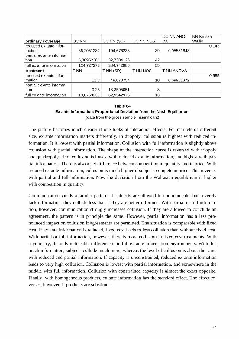
37

ordinary coverage OC NN OC NN (SD) OC NN NOS OC NN ANO-VA

NN Kruskal Wallis

reduced ex ante infor-mation 36,2051282 104,676238 39 0,05581643

0,143

partial ex ante informa-tion 5,80952381 32,7304126 42

full ex ante information 124,727273 384,742986 55 treatment T NN T NN (SD) T NN NOS T NN ANOVA reduced ex ante infor-mation 11,3 49,073754 10 0,69951372

0,585

partial ex ante informa-tion -0,25 18,3595051 8

full ex ante information 19,0769231 62,9542976 13

Table 64 Ex ante Information: Proportional Deviation from the Nash Equilibrium

(data from the gross sample insignificant)

The picture becomes much clearer if one looks at interaction effects. For markets of different size, ex ante information matters differently. In duopoly, collusion is highest with reduced in-formation. It is lowest with partial information. Collusion with full information is slightly above collusion with partial information. The shape of the interaction curve is reversed with triopoly and quadropoly. Here collusion is lowest with reduced ex ante information, and highest with par-tial information. There is also a net difference between competition in quantity and in price. With reduced ex ante information, collusion is much higher if subjects compete in price. This reverses with partial and full information. Now the deviation from the Walrasian equilibrium is higher with competition in quantity.

Communication yields a similar pattern. If subjects are allowed to communicate, but severely lack information, they collude less than if they are better informed. With partial or full informa-tion, however, communication strongly increases collusion. If they are allowed to conclude an agreement, the pattern is in principle the same. However, partial information has a less pro-nounced impact on collusion if agreements are permitted. The situation is comparable with fixed cost. If ex ante information is reduced, fixed cost leads to less collusion than without fixed cost. With partial or full information, however, there is more collusion in fixed cost treatments. With asymmetry, the only noticeable difference is in full ex ante information environments. With this much information, subjects collude much more, whereas the level of collusion is about the same with reduced and partial information. If capacity is unconstrained, reduced ex ante information leads to very high collusion. Collusion is lowest with partial information, and somewhere in the middle with full information. Collusion with constrained capacity is almost the exact opposite. Finally, with homogeneous products, ex ante information has the standard effect. The effect re-verses, however, if products are substitutes.

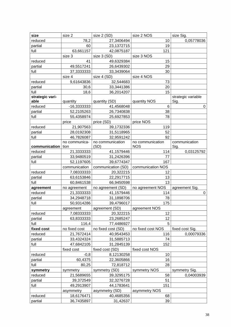
38

size size 2 size 2 (SD) size 2 NOS size Sig. reduced 78,2 27,3406494 10 0,05778036partial 60 23,1372715 19 full 63,661157 42,0875187 121 size 3 size 3 (SD) size 3 NOS reduced 41 49,6329384 15 partial 49,5517241 26,6439302 29 full 37,3333333 33,3439064 30 size 4 size 4 (SD) size 4 NOS reduced 9,61643836 32,544683 73 partial 30,6 33,3441386 20 full 18,6 36,2014207 15 strategic vari-able quantity quantity (SD) quantity NOS

strategic variable Sig.

reduced -16,3333333 41,4568048 6 0partial 52,2105263 26,7340838 38 full 55,4358974 25,6927853 78 price price (SD) price NOS reduced 21,907563 39,1732336 119 partial 28,0192308 31,5118965 52 full 46,7826087 32,9591242 92

communication no communica-tion

no communication (SD)

no communication NOS

communication Sig.

reduced 21,3333333 41,1579446 114 0,03125792partial 33,9480519 31,2426396 77 full 52,1197605 39,6774347 167 communication communication (SD) communication NOS reduced 7,08333333 20,322215 12 partial 63,6153846 22,2917715 13 full 60,8461538 66,9450598 13 agreement no agreement no agreement (SD) no agreement NOS agreement Sig. reduced 21,3333333 41,1579446 114 0partial 34,2948718 31,1898706 78 full 50,9314286 39,4796017 175 agreement agreement (SD) agreement NOS reduced 7,08333333 20,322215 12 partial 63,8333333 23,2685247 12 full 116,4 77,4486927 5 fixed cost no fixed cost no fixed cost (SD) no fixed cost NOS fixed cost Sig. reduced 21,7672414 40,9543453 116 0,00079336partial 33,4324324 31,5885713 74 full 47,6842105 31,2845139 152 fixed cost fixed cost (SD) fixed cost NOS reduced -0,8 8,12130258 10 partial 60,4375 22,3605866 16 full 80,25 72,818712 28 symmetry symmetry symmetry (SD) symmetry NOS symmetry Sig. reduced 21,5689655 39,3295175 58 0,04003939partial 39,372549 32,3276728 51 full 49,2913907 44,1783641 151 asymmetry asymmetry (SD) asymmetry NOS reduced 18,6176471 40,4685356 68 partial 36,7435897 31,42637 39

39

full 70,7586207 20,7547846 29 capacity unconstrained unconstrained (SD) unconstrained NOS capacity Sig. reduced 71,56 45,9547604 25 0partial 44,5 24,63737 52 full 57,738255 41,5450579 149 constrained constrained (SD) constrained NOS reduced 7,20792079 25,3957937 101 partial 29,6578947 38,2532643 38 full 28,7741935 36,0820451 31 homogeneity homogeneous homogeneous (SD) homogeneous NOS homogeneity Sig. reduced 6,8 27,5294947 105 0partial 32,5324675 30,6545199 77 full 49,722973 44,4867665 148 heterogeneous heterogeneous (SD) heterogeneous NOS reduced 85,8571429 22,3299926 21 partial 72 9,97496867 13 full 66,75 23,7459674 32

Table 65 Ex ante Information: Interaction Effects


2. Role of Feedback

At the aggregate level, ex ante and feedback information have similar effects. The deviation from the Walrasian equilibrium is smallest if feedback is reduced. It increases with partial feed-back, and it is highest with full feedback. As with ex ante information, the aggregate effect on deviations from the Nash equilibrium is less obvious. The only weakly significant result is in the ordinary coverage sample. It is the same as with the Walrasian equilibrium.

The distinction between partial and full is the same as with ex ante information. Feedback is full if subjects know their competitors’ profits. It is partial if they only know their own profit. Again the category of reduced feedback is less strictly defined. It encompasses all situations where sub-jects get even less feedback.


reduced feedback 6,51898734 30,5839998 79 0 0partial feedback 37,5426357 35,5630657 258 full feedback 57,3963964 45,5725753 111

ordinary coverage OC CW OC CW (SD) OC CW NOS OC CW ANO-VA

reduced feedback -0,57894737 23,274716 57 0 0partial feedback 22,4015748 31,2651893 127 full feedback 40,4150943 25,5150287 53 treatment T CW T CW (SD) T CW NOS T CW ANOVA reduced feedback 5,33333333 58,7934237 6 0,1014702 0,238partial feedback 40,0285714 38,6678813 35 full feedback 43,7368421 31,2940216 19

Table 66 Feedback: Normalized Deviation from the Walrasian Equilibrium

40


reduced feedback -85,6666667 77,6908403 6 0,57446048 0,009partial feedback -19,7142857 171,490623 35 full feedback -27,4736842 76,9670697 19

Table 67

Feedback: Normalized Deviation from the Nash Equilibrium (data from the gross and ordinary coverage samples insignificant)

ordinary cover-age OC NN OC NN (SD) OC NN NOS OC NN ANOVA

NN Kruskal Wal-lis

reduced feedback -2,66666667 4,9244289 9 0,08515388 0,022partial feedback 46,4867257 252,181876 113 full feedback 156,108696 413,03711 46 treatment T NN T NN (SD) T NN NOS T NN ANOVA reduced feedback -27,8333333 30,6099113 6 0,56795273 0,021partial feedback -6,0625 41,6505722 32 full feedback -3,66666667 64,9823505 18

Table 68

Feedback: Proportional Deviation from the Nash Equilibrium (data from the gross sample insignificant)

As with ex ante information, feedback is mainly relevant through its interaction with other treat-ment variables. If buyers are human, going from reduced to partial feedback has a much smaller effect on collusion. If subjects are allowed to communicate, the effect of partial feedback is small, but the effect of full feedback is very large. The opposite is true if subjects cannot com-municate. This pattern is even more pronounced if they are allowed to conclude an agreement. In a stranger design feedback is almost irrelevant. From this it follows that subjects use feedback mainly as a tool for backing collusion, not as one for learning how to interact. If interaction is simultaneous, feedback has the standard effects. In sequential interaction, however, collusion is high with reduced and with full feedback, and it is low with partial feedback.

If there is no fixed cost, feedback has the usual effects. With fixed cost, however, collusion is much higher with reduced and with full feedback. Although results are only weakly significant, it is also interesting to look at the interaction with surplus. If gains from collusion are high since most of the surplus is with consumers, feedback has the standard effects. With a symmetric dis-tribution of the surplus between sellers and buyers, going from partial to full feedback no longer increases collusion. If most of the surplus is with producers anyhow, collusion even drops if one goes from partial to full feedback. Finally, if products are homogeneous, feedback has the usual effects. With substitutes, however, collusion goes down if one goes from partial to full feedback.

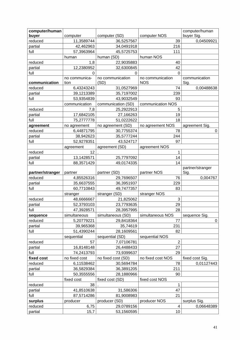
41

computer/human buyer computer computer (SD) computer NOS

computer/human buyer Sig.

reduced 11,3589744 36,5257567 39 0,04509921partial 42,462963 34,0491918 216 full 57,3963964 45,5725753 111 human human (SD) human NOS reduced 1,8 22,9035883 40 partial 12,2380952 32,6300845 42 full 0 0 0

communication no communica-tion

no communication (SD)

no communication NOS

communication Sig.

reduced 6,43243243 31,0527969 74 0,00488638partial 39,1213389 35,7197002 239 full 53,9354839 43,9032549 93 communication communication (SD) communication NOS reduced 7,8 25,2922913 5 partial 17,6842105 27,166263 19 full 75,2777778 51,0222622 18 agreement no agreement no agreement (SD) no agreement NOS agreement Sig. reduced 6,44871795 30,7755374 78 0partial 38,942623 35,5777244 244 full 52,9278351 43,524717 97 agreement agreement (SD) agreement NOS reduced 12 . 1 partial 13,1428571 25,7797092 14 full 88,3571429 49,0174335 14

partner/stranger partner partner (SD) partner NOS partner/stranger Sig.

reduced 4,85526316 29,7696507 76 0,004767partial 35,6637555 36,3951937 229 full 60,7710843 49,7477357 83 stranger stranger (SD) stranger NOS reduced 48,6666667 21,825062 3 partial 52,3793103 23,7793635 29 full 47,3928571 28,3957995 28 sequence simultaneous simultaneous (SD) simultaneous NOS sequence Sig. reduced 5,20779221 29,8418364 77 0partial 39,965368 35,74619 231 full 51,4390244 28,1609561 82 sequential sequential (SD) sequential NOS reduced 57 7,07106781 2 partial 16,8148148 26,4488433 27 full 74,2413793 73,9399637 29 fixed cost no fixed cost no fixed cost (SD) no fixed cost NOS fixed cost Sig. reduced 6,11538462 30,5694784 78 0,01127443partial 36,5829384 36,3891205 211 full 50,3555556 28,1880966 90 fixed cost fixed cost (SD) fixed cost NOS reduced 38 . 1 partial 41,8510638 31,586306 47 full 87,5714286 81,9008983 21 surplus producer producer (SD) producer NOS surplus Sig. reduced 6,75 29,0789156 4 0,06648389partial 15,7 53,1560595 10

42

full -2 15,5563492 2 symmetric symmetric (SD) symmetric NOS reduced 2,64102564 26,6916971 39 partial 31,8701299 31,8864559 77 full 29,125 23,5962568 16 consumer consumer (SD) consumer NOS reduced 10,6944444 34,6969076 36 partial 41,374269 35,3614984 171 full 64,4444444 46,6943471 90 capacity unconstrained unconstrained (SD) unconstrained NOS capacity Sig. reduced 24,0909091 49,451905 11 0,04256421partial 53,6241611 29,4896859 149 full 60,9659091 48,3346688 88 constrained constrained (SD) constrained NOS reduced 3,67647059 25,7887174 68 partial 15,559633 31,1984185 109 full 43,7391304 29,9927527 23 homogeneity homogeneous homogeneous (SD) homogeneous NOS homogeneity Sig. reduced 2,67123288 27,9285073 73 partial 30,793578 32,8133747 218 0full 53,3291139 52,0031364 79 heterogeneous heterogeneous (SD) heterogeneous NOS reduced 53,3333333 22,6686274 6 partial 74,325 26,4772641 40 full 67,4375 20,4654508 32

Table 69 Feedback: Interaction Effects


3. Neutral vs. Market Frame

In oligopoly experiments, it is standard to tell subjects that they are sellers in a market. Some experimenters wondered whether the explicit frame has an impact on the degree of collusion. This is indeed the case, but in a surprising direction. If subjects are given the underlying game in a neutral frame, cooperation (collusion) rates go up substantially.


market frame 35,8543046 40,9771246 453 0,0182041 0,004neutral frame 57,2380952 24,9116534 21 ordinary coverage OC CW OC CW (SD) OC CW NOS OC CW ANOVA market frame 18,814346 30,5160302 237 0 0neutral frame 50,0714286 22,1062619 14

Table 70 Frame: Normalized Deviation from the Walrasian Equilibrium

(no treatment data available)

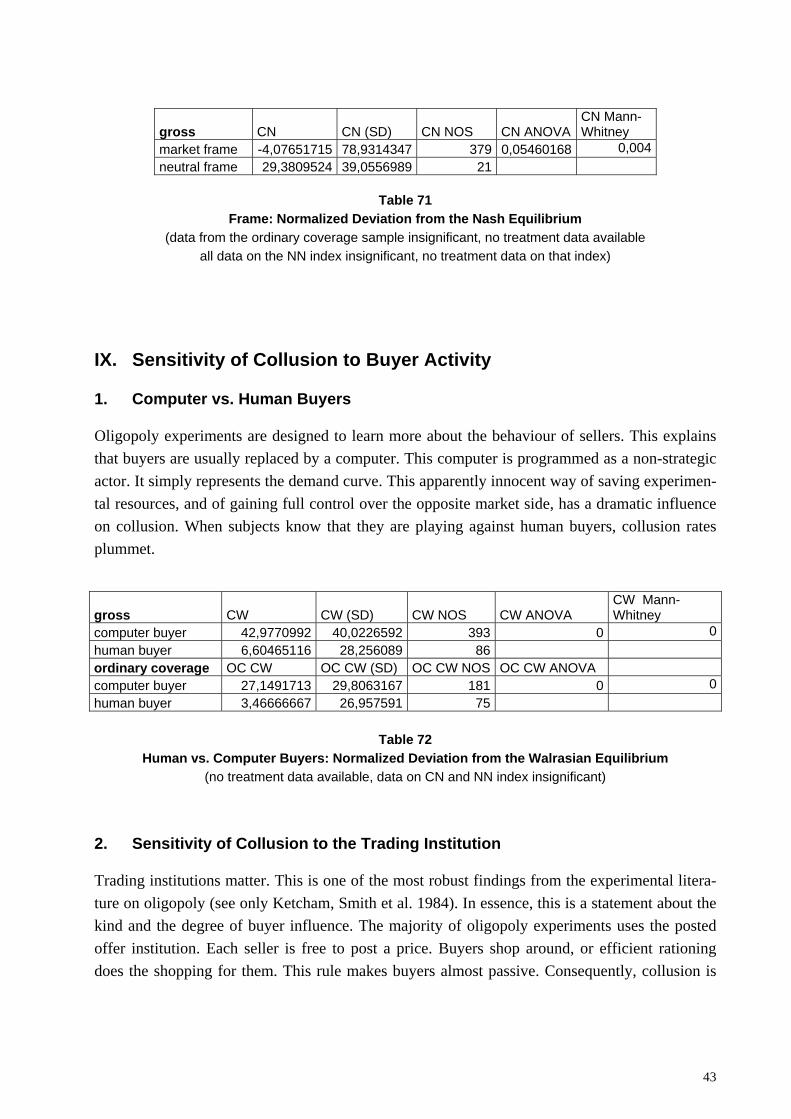
43


market frame -4,07651715 78,9314347 379 0,05460168 0,004 neutral frame 29,3809524 39,0556989 21

Table 71

Frame: Normalized Deviation from the Nash Equilibrium (data from the ordinary coverage sample insignificant, no treatment data available

all data on the NN index insignificant, no treatment data on that index)

IX. Sensitivity of Collusion to Buyer Activity

1. Computer vs. Human Buyers

Oligopoly experiments are designed to learn more about the behaviour of sellers. This explains that buyers are usually replaced by a computer. This computer is programmed as a non-strategic actor. It simply represents the demand curve. This apparently innocent way of saving experimen-tal resources, and of gaining full control over the opposite market side, has a dramatic influence on collusion. When subjects know that they are playing against human buyers, collusion rates plummet.


computer buyer 42,9770992 40,0226592 393 0 0human buyer 6,60465116 28,256089 86 ordinary coverage OC CW OC CW (SD) OC CW NOS OC CW ANOVA computer buyer 27,1491713 29,8063167 181 0 0human buyer 3,46666667 26,957591 75

Table 72 Human vs. Computer Buyers: Normalized Deviation from the Walrasian Equilibrium

(no treatment data available, data on CN and NN index insignificant)

2. Sensitivity of Collusion to the Trading Institution

Trading institutions matter. This is one of the most robust findings from the experimental litera-ture on oligopoly (see only Ketcham, Smith et al. 1984). In essence, this is a statement about the kind and the degree of buyer influence. The majority of oligopoly experiments uses the posted offer institution. Each seller is free to post a price. Buyers shop around, or efficient rationing does the shopping for them. This rule makes buyers almost passive. Consequently, collusion is

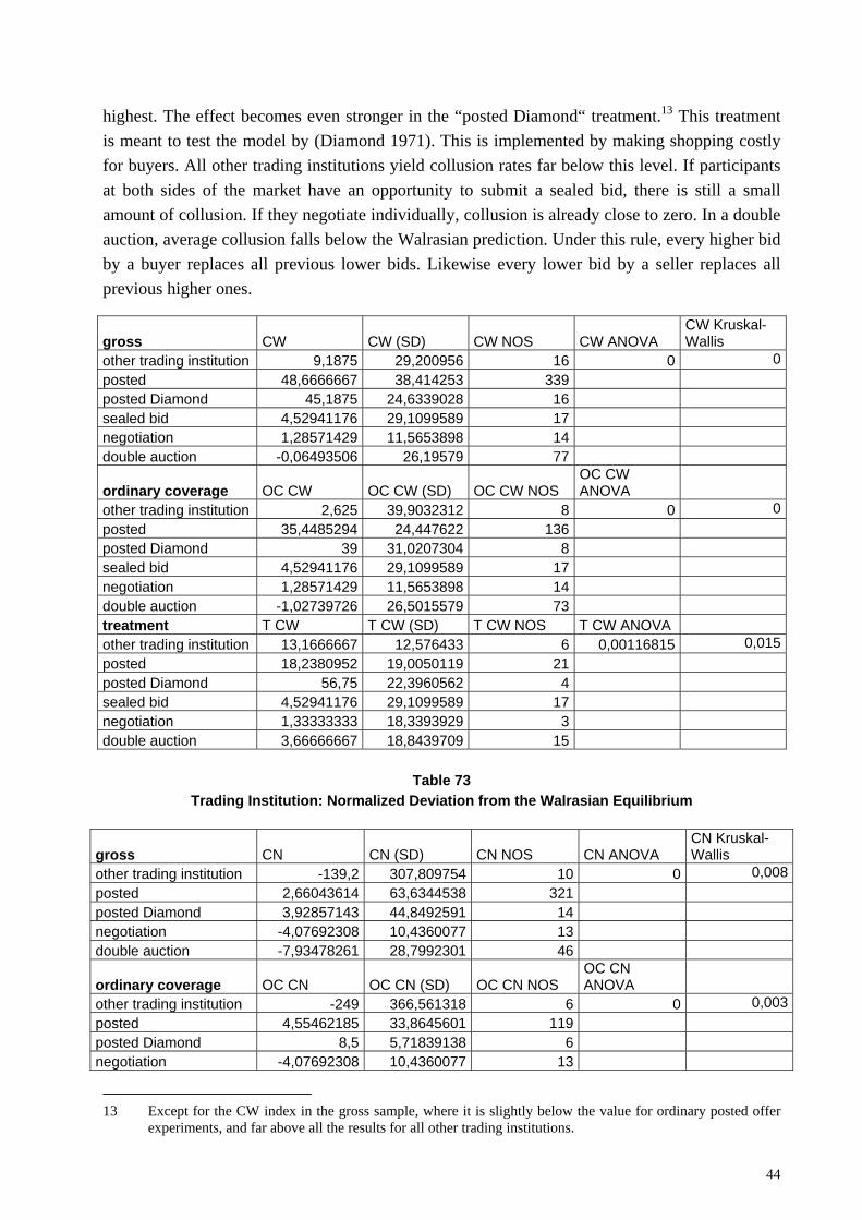
44

highest. The effect becomes even stronger in the “posted Diamond“ treatment.13 This treatment is meant to test the model by (Diamond 1971). This is implemented by making shopping costly for buyers. All other trading institutions yield collusion rates far below this level. If participants at both sides of the market have an opportunity to submit a sealed bid, there is still a small amount of collusion. If they negotiate individually, collusion is already close to zero. In a double auction, average collusion falls below the Walrasian prediction. Under this rule, every higher bid by a buyer replaces all previous lower bids. Likewise every lower bid by a seller replaces all previous higher ones.


other trading institution 9,1875 29,200956 16 0 0posted 48,6666667 38,414253 339 posted Diamond 45,1875 24,6339028 16 sealed bid 4,52941176 29,1099589 17 negotiation 1,28571429 11,5653898 14 double auction -0,06493506 26,19579 77

ordinary coverage OC CW OC CW (SD) OC CW NOS OC CW ANOVA

other trading institution 2,625 39,9032312 8 0 0posted 35,4485294 24,447622 136 posted Diamond 39 31,0207304 8 sealed bid 4,52941176 29,1099589 17 negotiation 1,28571429 11,5653898 14 double auction -1,02739726 26,5015579 73 treatment T CW T CW (SD) T CW NOS T CW ANOVA other trading institution 13,1666667 12,576433 6 0,00116815 0,015posted 18,2380952 19,0050119 21 posted Diamond 56,75 22,3960562 4 sealed bid 4,52941176 29,1099589 17 negotiation 1,33333333 18,3393929 3 double auction 3,66666667 18,8439709 15

Table 73 Trading Institution: Normalized Deviation from the Walrasian Equilibrium

gross CN CN (SD) CN NOS CN ANOVA CN Kruskal-Wallis

other trading institution -139,2 307,809754 10 0 0,008posted 2,66043614 63,6344538 321 posted Diamond 3,92857143 44,8492591 14 negotiation -4,07692308 10,4360077 13 double auction -7,93478261 28,7992301 46

ordinary coverage OC CN OC CN (SD) OC CN NOS OC CN ANOVA

other trading institution -249 366,561318 6 0 0,003posted 4,55462185 33,8645601 119 posted Diamond 8,5 5,71839138 6 negotiation -4,07692308 10,4360077 13

13 Except for the CW index in the gross sample, where it is slightly below the value for ordinary posted offer

experiments, and far above all the results for all other trading institutions.

45

double auction -9,8372093 28,7409864 43 treatment T CN T CN (SD) T CN NOS T CN ANOVA posted 2,61538462 33,0493027 13 0,01841942 0,022posted Diamond 55,5 22,6936114 4 negotiation -9 5,65685425 2 double auction -26,1428571 51,6540691 7

Table 74 Trading Institution: Normalized Deviation from the Nash Equilibrium

gross NN NN (SD) NN NOS NN ANOVA NN Kruskal-Wallis

other trading institution -85,3333333 73,9963963 6 0 0posted 38,9903846 173,147159 312 posted Dia-mond 271,25 613,814576 16

negotiation -1,61538462 7,03015483 13 double auction 4,725 43,3814255 40 ordinary cov-erage OC NN OC NN (SD) OC NN NOS OC NN ANOVA

other trading institution -85,3333333 73,9963963 6 0 0,011posted 76,6869565 273,718429 115 posted Dia-mond 488 836,420776 8

negotiation -1,61538462 7,03015483 13 double auction 4,72972973 45,1470736 37 treatment T NN T NN (SD) T NN NOS T NN ANOVA posted 56,9230769 154,47139 13 0,91419845 0,094posted Dia-mond 63 26,0895892 4

negotiation -1,5 0,70710678 2 double auction 33,4285714 104,485816 7

Table 75 Trading Institution: Proprotional Deviation from the Nash Equilibrium

3. Collusion under Conditions of Demand Inertia

In reality, demand is hardly ever perfectly elastic. Buyers hold to their buying habits as long as a competing offer is not clearly more attractive in qualitative terms, or substantially cheaper. Ex-perimenters have tested markets with such demand inertia. The result is as one would expect. Market outcomes are further away from both the Walrasian and the Nash predictions.

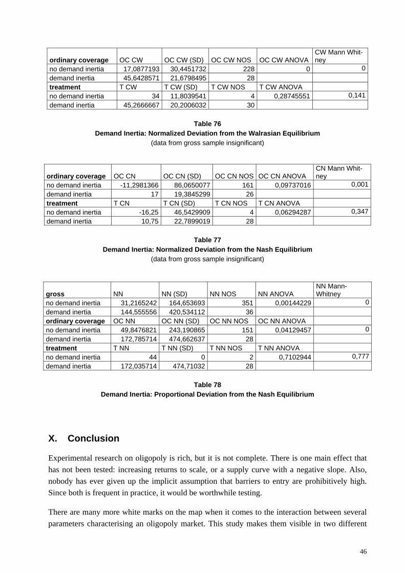
46

ordinary coverage OC CW OC CW (SD) OC CW NOS OC CW ANOVA CW Mann Whit-ney

no demand inertia 17,0877193 30,4451732 228 0 0demand inertia 45,6428571 21,6798495 28 treatment T CW T CW (SD) T CW NOS T CW ANOVA no demand inertia 34 11,8039541 4 0,28745551 0,141demand inertia 45,2666667 20,2006032 30

Table 76 Demand Inertia: Normalized Deviation from the Walrasian Equilibrium

(data from gross sample insignificant)

ordinary coverage OC CN OC CN (SD) OC CN NOS OC CN ANOVA

CN Mann Whit-ney

no demand inertia -11,2981366 86,0650077 161 0,09737016 0,001demand inertia 17 19,3845299 26 treatment T CN T CN (SD) T CN NOS T CN ANOVA no demand inertia -16,25 46,5429909 4 0,06294287 0,347demand inertia 10,75 22,7899019 28

Table 77 Demand Inertia: Normalized Deviation from the Nash Equilibrium

(data from gross sample insignificant)


no demand inertia 31,2165242 164,653693 351 0,00144229 0demand inertia 144,555556 420,534112 36 ordinary coverage OC NN OC NN (SD) OC NN NOS OC NN ANOVA no demand inertia 49,8476821 243,190865 151 0,04129457 0demand inertia 172,785714 474,662637 28 treatment T NN T NN (SD) T NN NOS T NN ANOVA no demand inertia 44 0 2 0,7102944 0,777demand inertia 172,035714 474,71032 28

Table 78 Demand Inertia: Proportional Deviation from the Nash Equilibrium

X. Conclusion

Experimental research on oligopoly is rich, but it is not complete. There is one main effect that has not been tested: increasing returns to scale, or a supply curve with a negative slope. Also, nobody has ever given up the implicit assumption that barriers to entry are prohibitively high. Since both is frequent in practice, it would be worthwhile testing.

There are many more white marks on the map when it comes to the interaction between several parameters characterising an oligopoly market. This study makes them visible in two different

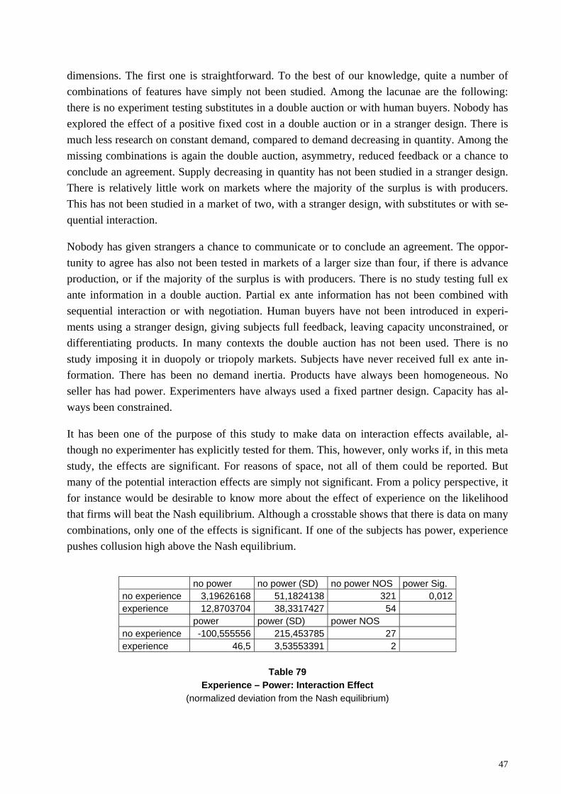
47

dimensions. The first one is straightforward. To the best of our knowledge, quite a number of combinations of features have simply not been studied. Among the lacunae are the following: there is no experiment testing substitutes in a double auction or with human buyers. Nobody has explored the effect of a positive fixed cost in a double auction or in a stranger design. There is much less research on constant demand, compared to demand decreasing in quantity. Among the missing combinations is again the double auction, asymmetry, reduced feedback or a chance to conclude an agreement. Supply decreasing in quantity has not been studied in a stranger design. There is relatively little work on markets where the majority of the surplus is with producers. This has not been studied in a market of two, with a stranger design, with substitutes or with se-quential interaction.

Nobody has given strangers a chance to communicate or to conclude an agreement. The oppor-tunity to agree has also not been tested in markets of a larger size than four, if there is advance production, or if the majority of the surplus is with producers. There is no study testing full ex ante information in a double auction. Partial ex ante information has not been combined with sequential interaction or with negotiation. Human buyers have not been introduced in experi-ments using a stranger design, giving subjects full feedback, leaving capacity unconstrained, or differentiating products. In many contexts the double auction has not been used. There is no study imposing it in duopoly or triopoly markets. Subjects have never received full ex ante in-formation. There has been no demand inertia. Products have always been homogeneous. No seller has had power. Experimenters have always used a fixed partner design. Capacity has al-ways been constrained.

It has been one of the purpose of this study to make data on interaction effects available, al-though no experimenter has explicitly tested for them. This, however, only works if, in this meta study, the effects are significant. For reasons of space, not all of them could be reported. But many of the potential interaction effects are simply not significant. From a policy perspective, it for instance would be desirable to know more about the effect of experience on the likelihood that firms will beat the Nash equilibrium. Although a crosstable shows that there is data on many combinations, only one of the effects is significant. If one of the subjects has power, experience pushes collusion high above the Nash equilibrium.

no power no power (SD) no power NOS power Sig. no experience 3,19626168 51,1824138 321 0,012 experience 12,8703704 38,3317427 54 power power (SD) power NOS no experience -100,555556 215,453785 27 experience 46,5 3,53553391 2

Table 79

Experience – Power: Interaction Effect (normalized deviation from the Nash equilibrium)

48

A closer look at the data demonstrates why further research on interaction effects is a desidera-tum. In the critical cell, the effect is based on just two observations. It has only become signifi-cant since the impact of experience is dramatic. This implies that explicit tests of interaction ef-fects should be able to establish many more of them. This study, and the data bank behind it, may help experimenters build expectations about the direction of the interaction effects, and where they are particularly likely to be found.

49

References

ALGER, DAN (1987). “Laboratory Tests of Equilibrium Predictions with Disequilibrium Data.“

Review of Economic Studies 54: 105-145.

ALLEN, BETH and MARTIN HELLWIG (1986a). Bertrand-Edgeworth Oligopoly in Large Markets.“ Review of Economic Studies 53: 175-204.

ALLEN, BETH and MARTIN HELLWIG (1986b). “Price-Setting Firms and the Oligopolistic Foun-dations of Perfect Competition.“ American Economic Association Papers and Proceedings 76: 387-392.

ALTAVILLA, CARLO, LUIGI LUINI and PATRIZIA SBRIGLIA (2005). Social Learning in Market Games http://www.econ-pol.unisi.it/labsi/labsi_paper/labsi3.pdf.

ANDERHUB, VITAL, WERNER GÜTH, ULRICH KAMECKE and HANS-THEO NORMANN (2003). “Ca-pacity Choices and Price Competition in Experimental Markets.“ Experimental Economics 6: 27-52.

AUMANN, ROBERT J. and LLOYD S. SHAPLEY (1994). Long Term Competition - A Game Theo-retic Analysis. Collected Papers I. Robert J. Aumann. Cambridge, MIT Press: 395-409.

BENSON, BRUCE L. and M.D. FAMINOW (1988). “The Impact of Experience on Prices and Profits in Experimental Duopoly Markets.“ Journal of Economic Behavior & Organization 9: 345-365.

BERTRAND, JOSEPH LOUIS FRANCOIS (1883). “Théorie mathématique de la richesse sociale par León Walras. Recherches sur les principes mathématiques de la théorie des richesses par Augustin Cournot.“ Journal des savants 67: 499-508.

BORTZ, JÜRGEN (2005). Statistik für Human- und Sozialwissenschaftler. Heidelberg, Springer.

BOSCH-DOMÈNECH, ANTONI and NICOLAAS J. VRIEND (2003). “Imitation of Successful Behavior in Cournot Markets.“ Economic Journal 113: 495-524.

CAPRA, MONICA C., JACOB K. GOEREE, ROSARIO GOMEZ and CHARLES A. HOLT (2002). “Learn-ing and Noisy Equilibrium Behavior in an Experimental Study of Imperfect Price Competi-tion.“ International Economic Review 43: 613-636.

CASON, TIMOTHY N. and DOUGLAS D. DAVIS (1995). “Price Communication in a Multi-Market Context. An Experimental Investigation.“ Review of Industrial Organization 10: 769-787.

CHAMBERLIN, EDWARD (1933). The Theory of Monopolistic Competition. Cambridge,, Harvard University Press.

50

COURNOT, ANTOINE-AUGUSTIN (1838). Recherches sur les principes mathématiques de la théorie des richesses. Paris,, Libraririe des sciences politiques et sociales M. Riveáre & cie.

COX, JAMES C. and MARK WALKER (1998). “Learning to Play Cournot Duopoly Strategies.“ Journal of Economic Behavior & Organization 36: 141-161.

CRAWFORD, VINCENT (1998). “A Survey of Experiments on Communication via Cheap Talk.“ Journal of Economic Theory 78(2): 286-298.

DAUGHETY, ANDREW F. and ROBERT FORSYTHE (1987). “The Effects of Industry-Wide Price Regulation on Industrial Organization.“ Journal of Law, Economics and Organization 3: 397-434.

DAVIDSON, CARL and RAYMOND J. DENECKERE (1986). “Long-Run Competition in Capacity, Short-Run Competition in Price, and the Cournot Model.“ Rand Journal of Economics 17: 404-415.

DAVIS, DOUGLAS D. and CHARLES A. HOLT (1993). Experimental Economics. Princeton, NJ, Princeton Univ. Press.

DAVIS, DOUGLAS D., ROBERT J. REILLY and BART WILSON (2003). “Cost Structures and Nash Play in Repeated Cournot Games.“ Experimental Economics 6: 209-226.

DAVIS, DOUGLAS and BART WILSON (2005). “Differentiated Product Competition and the Anti-trust Logit Model. An Experimental Analysis.“ Journal of Economic Behavior & Organi-zation 57: 89-113.

DIAMOND, PETER (1971). “A Model of Price Adjustments.“ Journal of Economic Theory 3: 156-168.

EDGEWORTH, FRANCIS (1897). “La Teoria Pura del Monopolio.“ Giornale degli Economisti 40: 13-31.

FOURAKER, LAWRENCE E. and SIDNEY SIEGEL (1963). Bargaining Behavior. New York,, McGraw-Hill.

FRIEDMAN, DANIEL (1969). “On Experimental Research in Oligopoly.“ Review of Economic Studies 36: 399-415.

FRIEDMAN, MILTON (1953). Essays in Positive Economics. [Chicago], University of Chicago Press.

FUDENBERG, DREW and JEAN TIROLE (1991). Game Theory. Cambridge, Mass., MIT Press.

HAYS, WILLIAM LEE (1994). Statistics. Fort Worth, Harcourt College Publishers.

51

HOGGATT, AUSTIN CURWOOD (1959). “An Experimental Business Game.“ Behavioral Science 4: 192-203.

HOLT, CHARLES A. (1995). Industrial Organization. A Survey of Laboratory Research. Hand-book of Experimental Economics. John H. Kagel und Alvin E. Roth. Princeton, Princeton University Press: 349-443.

HOLT, CHARLES A. and FERNANDO SOLIS-SOBERON (1992). “The Calculation of Equilibrium Mixed Strategies in Posted-Offer Auctions.“ Research in Experimental Economics 5: 189-228.

HUCK, STEFFEN, HANS-THEO NORMANN and JÖRG OECHSSLER (2004). “Two are Few and Four are Many. Number Effects in Experimental Oligopolies.“ Journal of Economic Behavior & Organization 53: 435-446.

ISAAC, R. MARK, VALÉRIE RAMEY and ARLINGTON W. WILLIAMS (1984). “The Effects of Market Organization on Conspiracy in Restraints of Trade.“ Journal of Economic Behavior & Or-ganization 5: 191-222.

KETCHAM, JON, VERNON L. SMITH and ARLINGTON W. WILLIAMS (1984). “A Comparison of Posted-Offer and Double-Auction Pricing Institutions.“ Review of Economic Studies 51: 595-614.

KREPS, DAVID M. and JOSE ALEXANDRE SCHEINKMAN (1983). “Quantity Precommitment and Bertrand Competition Yields Cournot Outcomes.“ Bell Journal of Economics 14: 326-337.

LUPI, PAOLO and PATRIZIA SBRIGLIA (2003). “Exploring Human Behaviour and Learning in Ex-perimental Cournot Settings.“ Rivista Internazionale di Studi Sociali 51: 373-397.

NAGEL, ROSEMARIE and NICOLAAS J. VRIEND (1999a). “An Experimental Study of Adaptive Be-haviour in an Oligopolistic Market Game.“ Journal of Evolutionary Economics 9: 27-65.

NAGEL, ROSEMARIE and NICOLAAS J. VRIEND (1999b). “Inexperienced and Experienced Players in an Oligopolistic Market Game with Minimal Information.“ Industrial and Corporate Change 8: 41-65.

OFFERMAN, THEO, JAN POTTERS and JOEP SONNEMANS (2002). “Imitation and Belief Learning in an Oligopoly Experiment.“ Review of Economic Studies 69: 973-997.

PLOTT, CHARLES R. (1982). “Industrial Organization. Theory and Experimental Economics.“ Journal of Economic Literature 20: 1485-1527.

PLOTT, CHARLES R. (1989). An Updated Review of Industrial Organization. Applications of Ex-perimental Methods. Handbook of Industrial Organization. Richard Schmalensee und Robert D. Willig. Amsterdam, North Holland: 1109-1176.

52

RASSENTI, STEPHEN, STANLEY S. REYNOLDS, VERNON L. SMITH and FERENC SZIDAROVSZKY (2000). “Adaptation Convergence of Behaviour in Repeated Experimental Cournot Games.“ Journal of Economic Behavior & Organization 41: 117-146.

SELTEN, REINHARD (1973). “A Simple Model of Imperfect Competition, Where Four Are Few and Six Are Many.“ International Journal of Game Theory 2: 141-201.

SELTEN, REINHARD (1978). “The Chain Store Paradox.“ Theory and Decision 9: 127-159.

SELTEN, REINHARD and HEINZ SAUERMANN (1959). “Ein Oligopolexperiment.“ Zeitschrift für die gesamte Staatswissenschaft 115: 427-471.

SELTEN, REINHARD and ROLF STOECKER (1986). “End Behavior in Sequences of Finite Prisoner's Dilemma Supergames.“ Journal of Economic Behavior & Organization 7: 47-70.

SHERMAN, ROGER (1969). “Risk Attitude and Cost Variability in a Capacity Choice Experi-ment.“ Review of Economic Studies 36: 453-466.

SHUBIK, MARTIN, GERRIT WOLF and SCOTT LOCKHART (1971). “An Artificial Player for a Busi-ness Market Game.“ Simulation and Games 2: 27-43.

SMITH, VERNON L. (1976). “Experimental Economics: Induced Value Theory.“ American Eco-nomic Review Papers and Proceedings 66: 274-279.

STACKELBERG, HEINRICH VON (1934). Marktform und Gleichgewicht. Wien und Berlin,, J. Springer.

SUETENS, SIGRID (2004). R&D Cooperation in Oligopoly with Spillovers. An Experimental Eco-nomics Approach. Literature Review

http://www.ua.ac.be/download.aspx?c=*TEWHI&n=14378&ct=009844&e=34935.

SUETENS, SIGRID and JAN POTTERS (2005). Bertrand Colludes More Than Cournot http://ideas.repec.org/p/ant/wpaper/2005037.html.

TIROLE, JEAN (1988). The Theory of Industrial Organization. Cambridge, Mass., MIT Press.

53

papers included in the meta-study

ABBINK, KLAUS and JORDI BRANDTS (2003). 24 http://www.iae-csic.uab.es/brandts/pub/24-revised.pdf.

ABBINK, KLAUS and JORDI BRANDTS (2005a). Collusion in Growing and Shrinking Markets. Empirical Evidence from Experimental Duopolies

http://www.nottingham.ac.uk/economics/cedex/papers/2005-03.pdf.

ABBINK, KLAUS and JORDI BRANDTS (2005b). “Price Competition under Cost Uncertainty. A Laboratory Analysis.“ Economic Inquiry 43: 636-648.

ABRAMS, ERIC, MARTIN SEFTON and ABDULLAH YAVAS (2000). “An Experimental Comparison of two Search Models.“ Economic Theory 16: 735-749.

ALTAVILLA, CARLO, LUIGI LUINI and PATRIZIA SBRIGLIA (2005). Social Learning in Market Games http://www.econ-pol.unisi.it/labsi/labsi_paper/labsi3.pdf.

ANDERHUB, VITAL, WERNER GÜTH, ULRICH KAMECKE and HANS-THEO NORMANN (2003). “Ca-pacity Choices and Price Competition in Experimental Markets.“ Experimental Economics 6: 27-52.

BAILEY, JEFF and STUART MESTELMAN (2002). Testing and Verifying Cournot and Bertrand Theories of Duopoly Markets

BOSCH-DOMÈNECH, ANTONI and NICOLAAS J. VRIEND (2003). “Imitation of Successful Behavior in Cournot Markets.“ Economic Journal 113: 495-524.

BRANDTS, JORDI and PABLO GUILLÉN (2004). Collusion into Fights in an Experiment with Price-Setting Firms and Production in Advance http://pareto.uab.es/wp/2004/61804.pdf.

BROWN KRUSE, JAMIE, STEPHEN RASSENTI, STANLEY S. REYNOLDS and VERNON L. SMITH (1994). “Bertrand-Edgeworth Competition in Experimental Markets.“ Econometrica 62: 343-371.

CAPRA, MONICA C., JACOB K. GOEREE, ROSARIO GOMEZ and CHARLES A. HOLT (2002). “Learn-ing and Noisy Equilibrium Behavior in an Experimental Study of Imperfect Price Competi-tion.“ International Economic Review 43: 613-636.

CARLSON, JOHN A. (1967). “The Stability of an Experimental Market with a Supply-Response Lag.“ Southern Economic Journal 33: 305-321.

CASON, TIMOTHY N. and DOUGLAS D. DAVIS (1995). “Price Communication in a Multi-Market Context. An Experimental Investigation.“ Review of Industrial Organization 10: 769-787.

54

CASON, TIMOTHY N. and DANIEL FRIEDMAN (2003). “Buyer Search and Price Dispersion. A Laboratory Study.“ Journal of Economic Theory 112: 232-260.

COOK, WILLIAM D. and E.C.H. VEENDORP (1975). “Six Markets in Search of an Auctioneer.“ Canadian Journal of Economics 8: 238-257.

CRÖSSMANN, HEINZ JÜRGEN (1982). Entscheidungsverhalten auf unvollkommenen Märkten. Frankfurt, Barudio.

DAUGHETY, ANDREW F. and ROBERT FORSYTHE (1987). Industrywide Regulation and the Forma-tion of Reputations. A Laboratory Analysis. Public Regulation. New Perspectives on Insti-tutions and Policies. Elizabeth E. Bailey. Cambridge, Mass., MIT Press: 347-398.

DAVIS, DOUGLAS (1996). “Consumer Search Costs and Market Performance.“ Economic Inquiry 34: 133-151.

DAVIS, DOUGLAS (1998). “Conspiracies and Secret Discounts in Laboratory Markets.“ Economic Journal 108: 736-756.

DAVIS, DOUGLAS D. (1999). “Advanced Production and Cournot Outcomes. An Experimental Investigation.“ Journal of Economic Behavior & Organization 40: 59-79.

DAVIS, DOUGLAS D. and ARLINGTON W. WILLIAMS (1986). “The Effects of Rent Asymmetries in Posted Offer Markets.“ Journal of Economic Behavior & Organization 7: 303-316.

DAVIS, DOUGLAS D. and BART WILSON (2003). Horizontal Merger, Strategic Buyers and Fixed Cost Synergies. An Experimental Investigation

http://www.people.vcu.edu/~dddavis/working%20papers/dw0803.pdf.

DAVIS, DOUGLAS and CHARLES A. HOLT (1994). “Market Power and Mergers in Laboratory Markets with Posted Prices.“ Rand Journal of Economics 25: 467-487.

DAVIS, DOUGLAS and BART WILSON (2000). “Firm-Specific Cost Savings and Market Power.“ Economic Theory 16: 545-565.

DIXON, HUW D., PATRIZIA SBRIGLIA and ERNESTO SOMMA (2003). Learning to Collude. An Ex-periment in Convergence and Equilibrium Selection in Oligopoly

http://papers.ssrn.com/sol3/papers.cfm?abstract_id=877231.

DOLBAER, F.G., L.B. LAVE, G. BOWMAN, A. LIEBERMAN, E. PRESCOTT, F. RUETTER and R. SHERMAN (1968). “Collusion in Oligopoly. An Experiment on the Effect of Numbers and Information.“ Quarterly Journal of Economics 82: 240-259.

DUFWENBERG, MARTIN and URI GNEEZY (2000). “Price Competition and Market Concentration. An Experimental Study.“ International Journal of Industrial Organization 18: 7-22.

55

DUFWENBERG, MARTIN, URI GNEEZY, JACOB K. GOEREE and ROSEMARIE NAGEL (2002). Price Floors and Competition http://www.ne.su.se/paper/wp02_13.pdf.

DUGAR, SUBHASISH (2005). Do Price-Matching Guarantees Facilitate Tacit Collusion? An Ex-perimental Study http://ssrn.com/abstract=655392.

DUGAR, SUBHASISH and TODD SORENSEN (2005). Hassle Costs, Price-Matching Guarantees and Price Competition. An Experiment http://ssrn.com/abstract=727324.

FAJFAR, PABLO (2005). Information and Competition in Cournot's Model. Evidence from the Laboratory http://ssrn.com/abstract=884231.

FEINBERG, ROBERT M. and THOMAS A. HUSTED (1993). “An Experimental Test of Discount-Rate Effects on Collusive Behaviour in Duopoly Markets.“ Journal of Industrial Economics 41: 153-160.

FEINBERG, ROBERT M. and ROGER SHERMAN (1988). “Mutual Forbearance under Experimental Conditions.“ Southern Economic Journal 54: 985-993.

FONSECA, MIGUEL A., STEFFEN HUCK and HANS-THEO NORMANN (2005). “Playing Cournot Al-though They Shouldn't.“ Economic Theory 25: 669-677.

FONSECA, MIGUEL A., WIELAND MÜLLER and HANS-THEO NORMANN (2005). Endogenous Tim-ing in Duopoly. Experimental Evidence

http://greywww.kub.nl:2080/greyfiles/center/2005/doc/77.pdf.

FOURAKER, LAWRENCE E. and SIDNEY SIEGEL (1963). Bargaining Behavior. New York, McGraw-Hill.

FRIEDMAN, JAMES W. and AUSTIN CURWOOD HOGGATT (1980). An Experiment in Noncoopera-tive Oligopoly. Greenwich, Conn., JAI Press.

GARCÍA GALLEGO, AURORA (1998). “Oligopoly Experimentation of Learning with Simulated Markets.“ Journal of Economic Behavior & Organization 35: 333-355.

GARCÍA GALLEGO, AURORA and NIKOLAOS GEORGANTZIS (2001). “Multiproduct Activity in an Experimental Differentiated Oligopoly.“ International Journal of Industrial Organization 19: 493-518.

GOODWIN, DAVID and STUART MESTELMAN (2003). Advance Production Duopolies and Posted Prices or Market-Clearing Prices

http://socserv.mcmaster.ca/econ/mceel/papers/KSDuopAllAug03.pdf.

GRETHER, DAVID M. and CHARLES R. PLOTT (1984). “The Effects of Market Practices in Oli-gopolistic Markets. An Experimental Examination of the Ethyl Case.“ Economic Inquiry 22: 479-507.

56

GÜTH, WERNER, WIELAND MÜLLER and YOSSI SPIEGEL (2006). “Noisy Leadership. An Experi-mental Approach.“ Games and Economic Behavior forthcoming.

HARSTAD, RONALD, STEPHEN MARTIN and HANS-THEO NORMANN (1998). Intertemporal Pricing Schemes. Experimental Tests of Consciously Parallel Behaviour in Oligopoly. Applied In-dustrial Economics. Louis Phlips. Cambridge, Cambridge University Press: 123-151.

HOFFMAN, ELIZABETH and CHARLES R. PLOTT (1981). “The Effect of Intertemporal Speculation on the Outcomes in Seller Posted Offer Auction Markets.“ Quarterly Journal of Economics 96: 223-242.

HOGGATT, AUSTIN CURWOOD (1959). “An Experimental Business Game.“ Behavioral Science 4: 192-203.

HOGGATT, AUSTIN CURWOOD (1969). “Response of Paid Student Subjects to Differential Behav-iour of Robots in Bifurcated Duopoly Games.“ Review of Economic Studies 36: 417-432.

HOLT, CHARLES A. (1985). “An Experimental Test of the Consistent-Conjectures Hypothesis.“ American Economic Review 75: 314-325.

HOLT, CHARLES A. and ANNE P. VILLAMIL (1986). “A Laboratory Experiment with a Singe-Person Cobweb.“ Atlantic Economic Journal 14/2: 51-54.

HONG, JAMES T. and CHARLES R. PLOTT (1982). “Rate Filing Policies for Inland Water Transpor-tation. An Experimental Approach.“ Bell Journal of Economics 13: 1-19.

HUCK, STEFFEN, WIELAND MÜLLER and HANS-THEO NORMANN (2001). “Stackelberg Beats Cournot. On Collusion and Efficiency in Experimental Markets.“ Economic Journal 111: 749-765.

HUCK, STEFFEN, WIELAND MÜLLER and HANS-THEO NORMANN (2002). “To Commit or Not to Commit. Endogenous Timing in Experimental Duopoly Markets.“ Games and Economic Behavior 38: 240-264.

HUCK, STEFFEN, WIELAND MÜLLER and HANS-THEO NORMANN (2004). “Strategic Delegation in Experimental Markets.“ International Journal of Industrial Organization 22: 561-574.

HUCK, STEFFEN, HANS-THEO NORMANN and JÖRG OECHSSLER (1999). “Learning in Cournot Oli-gopoly. An Experiment.“ Economic Journal 109: C80-C95.

HUCK, STEFFEN, HANS-THEO NORMANN and JÖRG OECHSSLER (2000). “Does Information About Competitor's Actions Increase or Decrease Competition in Experimental Oligopoly Mar-kets?“ International Journal of Industrial Organization 18: 39-57.

HUCK, STEFFEN, HANS-THEO NORMANN and JÖRG OECHSSLER (2001). “Market Volatility and Inequality in Earnings. Experimental Evidence.“ Economics Letters 70: 363-368.

57

HUCK, STEFFEN, HANS-THEO NORMANN and JÖRG OECHSSLER (2002). “Stability of the Cournot Process. Experimental Evidence.“ International Journal of Game Theory 31: 123-136.

HUCK, STEFFEN, HANS-THEO NORMANN and JÖRG OECHSSLER (2004). “Two are Few and Four are Many. Number Effects in Experimental Oligopolies.“ Journal of Economic Behavior & Organization 53: 435-446.

HUCK, STEFFEN and BRIAN WALLACE (2002). “Reciprocal Strategies and Aspiration Levels in a Cournot-Stackelberg Experiment.“ Economics Bulletin 3/3: 1-7.

ISAAC, R. MARK and CHARLES R. PLOTT (1981a). “The Opportunity for Conspiracy in Restraint of Trade. An Experimental Study.“ Journal of Economic Behavior & Organization 2: 1-30.

ISAAC, R. MARK and CHARLES R. PLOTT (1981b). “Price Controls and the Behavior of Auction Markets. An Experimental Examination.“ American Economic Review 71: 448-459.

ISAAC, R. MARK, VALÉRIE RAMEY and ARLINGTON W. WILLIAMS (1984). “The Effects of Market Organization on Conspiracy in Restraints of Trade.“ Journal of Economic Behavior & Or-ganization 5: 191-222.

JOHNSON, MICHAEL D. and CHARLES R. PLOTT (1989). “The Effect of Two Trading Institutions on Price Expectations and the Stability of Supply-Response Lag Markets.“ Journal of Eco-nomic Psychology 10: 189-216.

JULLIEN, CÉLINE and BERNARD RUFFIEUX (2001). “Innovation, avantages concurrentiels et con-currence. Une Analyse expérimentelle des incitations à innover et de l'efficacité des marchés en présence de chocs endogènes.“ Revue d'Économie Politique 111: 121-149.

KESER, CLAUDIA (1993). “Some Results of Experimental Duopoly Markets with Demand Iner-tia.“ Journal of Industrial Economics 41: 133-151.

KESER, CLAUDIA (2000). “Cooperation in Symmetric Duopolies with Demand Inertia.“ Interna-tional Journal of Industrial Organization 18: 23-38.

KÜBLER, DOROTHEA and WIELAND MÜLLER (2002). “Simultaneous and Sequential Price Com-petition in Heterogeneous Duopoly Markets. Experimental Evidence.“ International Jour-nal of Industrial Organization 20: 1437-1460.

MARTINI, GIANMARIA (2003). “Complexity and Individual Rationality in a Dynamic Duopoly. An Experimental Study.“ Research in Economics 57: 345-370.

MASON, CHARLES F. and OWEN R. PHILLIPS (1997). “Information and Cost Asymmetry in Ex-perimental Duopoly Markets.“ Review of Economics and Statistics 79: 290-299.

58

MASON, CHARLES F., OWEN R. PHILLIPS and CLIFFORD NOWELL (1992). “Duopoly Behavior in Asymmetric Markets. An Experimental Evaluation.“ Review of Economics and Statistics 74: 662-670.

MESTELMAN, STUART, DEBORAH WELLAND and DOUGLAS WELLAND (1987). “Advance Produc-tion in Posted Offer Markets.“ Journal of Economic Behavior & Organization 8: 249-264.

MESTELMAN, STUART and DOUGLAS WELLAND (1987). “Advance Production in Oral Double Auction Markets.“ Economics Letters 23: 43-48.

MESTELMAN, STUART and DOUGLAS WELLAND (1988). “Advance Production in Experimental Markets.“ Review of Economic Studies 55: 641-654.

MESTELMAN, STUART and DOUGLAS WELLAND (1991). “The Effects of Rent Asymmetries in Markets Characterized by Advance Production. A Comparison of Trading Institutions.“ Journal of Economic Behavior & Organization 15: 387-405.

MILLER, ROSS M., CHARLES R. PLOTT and VERNON L. SMITH (1977). “Intertemporal Competitive Equilibrium. An Empirical Study of Speculation.“ Quarterly Journal of Economics 91: 599-624.

MORGAN, JOHN, HENRIK ORZEN and MARTIN SEFTON (2006). “An Experimental Study of Price Dispersion.“ Games and Economic Behavior 54: 134-158.

MÜLLER, WIELAND (2006). “Allowing for Two Production Periods in the Cournot Duopoly. Ex-perimental Evidence.“ Journal of Economic Behavior & Organization 60: 100-111.

MUREN, ASTRI (2000). “Quantity Precommitment in an Experimental Oligopoly Market.“ Jour-nal of Economic Behavior & Organization 41: 147-157.

MUREN, ASTRI and ROGER PYDDOKE (1999). Does Collusion Without Communication Exist? http://ideas.repec.org/p/hhs/sunrpe/1999_0011.html.

MURPHY, JAMES L. (1966). “Effects of the Threat of Losses on Duopoly Bargaining.“ Quarterly Journal of Economics 80: 296-313.

OECHSSLER, JÖRG and FRANK SCHUHMACHER (2004). “The Limited Liability Effect in Experi-mental Duopoly Markets.“ International Journal of Industrial Organization 22: 163-184.

OFFERMAN, THEO, JAN POTTERS and JOEP SONNEMANS (2002). “Imitation and Belief Learning in an Oligopoly Experiment.“ Review of Economic Studies 69: 973-997.

ORZEN, HENRIK (2005). Concentration and Competition. An Experiment http://www.nottingham.ac.uk/economics/cedex/papers/2005-06.pdf.

59

PANTZ, KATINKA and ANTHONY ZIEGELMEYER (2004). Collaborative Networks in Experimental Triopolies ftp://papers.econ.mpg.de/esi/discussionpapers/2005-38.pdf.

PHILLIPS, OWEN R. and CHARLES F. MASON (1992). “Mutual Forbearance in Experimental Con-glomerate Markets.“ Rand Journal of Economics 23: 395-414.

PLOTT, CHARLES R. and VERNON L. SMITH (1978). “An Experimental Examination of Two Ex-change Institutions.“ Review of Economic Studies 45: 133-153.

PLOTT, CHARLES R. and JONATHAN T. UHL (1981). “Competitive Equilibrium with Middlemen. An Empirical Study.“ Southern Economic Journal 47: 1063-1071.

RASSENTI, STEPHEN, STANLEY S. REYNOLDS, VERNON L. SMITH and FERENC SZIDAROVSZKY (2000). “Adaptation Convergence of Behaviour in Repeated Experimental Cournot Games.“ Journal of Economic Behavior & Organization 41: 117-146.

RUFFLE, BRADLEY J. (2000). “Some Factors Affecting Demand Withholding in Posted-Offer Markets.“ Economic Theory 16: 529-544.

SAUERMANN, HEINZ and REINHARD SELTEN (1959). “Ein Oligopolexperiment.“ Zeitschrift für die gesamte Staatswissenschaft 115: 427-471.

SELTEN, REINHARD (1967a). Ein Oligopolexperiment mit Preisvariation und Investition. Beiträge zur experimentellen Wirtschaftsforschung. Ernst Sauermann. Tübingen, Mohr: 103-135.

SELTEN, REINHARD (1967b). Investitionsverhalten im Oligopolexperiment. Beiträge zur Experi-mentellen Wirtschaftsforschung I. Ernst Sauermann. Tübingen, Mohr: 60-102.

SELTEN, REINHARD (1970). Ein Marktexperiment. Beiträger zur experimentellen Wirtschaftsfor-schung II. Ernst Sauermann. Tübingen, Mohr: 33-98.

SELTEN, REINHARD and CLAUS C. BERG (1970). Drei experimentelle Oligopolspielserien mit kontinuierlichem Zeitablauf. Beiträge zur Experimentellen Wirtschaftsforschung II. Ernst Sauermann. Tübingen, Mohr: 162-221.

SHERMAN, ROGER (1971). “An Experiment on the Persistence of Price Collusion.“ Southern Eco-nomic Journal 37: 489-495.

SHERMAN, ROGER (1972). Oligopoly. An Empirical Approach. Lexington, Mass., Lexington Books.

SHUBIK, MARTIN, GERRIT WOLF and HERBERT B. EISENBERG (1972). “Some Experiences with an Experimental Oligopoly Business Game.“ General Systems 17: 61-74.

SMITH, VERNON L. and ARLINGTON W. WILLIAMS (1981). “On Nonbinding Price Controls in a Competitive Market.“ American Economic Review 71: 467-474.

60

SMITH, VERNON L. and ARLINGTON W. WILLIAMS (1982). “The Effects of Rent Asymmetries in Experimental Aucion Markets.“ Journal of Economic Behavior & Organization 3: 99-116.

SMITH, VERNON L., ARLINGTON W. WILLIAMS, W. KENNETH BRATTON and MICHAEL G. VAN-

NONI (1982). “Competitive Market Institutions. Double Auction vs. Sealed Bid-Offer.“ American Economic Review 72: 58-77.

STOECKER, ROLF (1980). Experimentelle Untersuchung des Entscheidungsverhaltens im Bert-rand-Oligopol. Bielefeld, Pfeffer.

SUETENS, SIGRID (2003). Does R& Cooperation Facilitate Price Collusion? An Experiment http://greywww.kub.nl:2080/greyfiles/center/2003/doc/99.pdf.

SUETENS, SIGRID (2005). “Cooperative and Noncooperative R&D in Experimental Duopoly Mar-kets.“ International Journal of Industrial Organization 23: 63-82.

WELLFORD, CHARISSA PEPIN (1990). Takeovers and Horizontal Mergers. Policy and Perform-ance. Ann Arbor, UMI.

WILLIAMS, ARLINGTON W. (1979). “Intertemporal Competitive Equilibrium. On Further Experi-mental Results.“ Research in Experimental Economics 1: 255-278.

WILLIAMS, ARLINGTON W. (1987). “The Formation of Price Forecasts in Experimental Markets.“ Journal of Money, Credit and Banking 19: 1-18.

WILLIAMS, ARLINGTON W. and VERNON L. SMITH (1984). “Cyclical Double-Auction Markets with and without Speculators.“ Journal of Business 57: 1-33.

WOLF, GERRIT and MARTIN SHUBIK (1975). “Teams Compared to Individuals in Duopoly Games with an Artifical Player.“ Southern Economic Journal 41: 635-648.

Documents

How Much Collusion? A Meta-Analysis On Oligopoly Experiments