Embed Size (px)
Citation preview

Lehrstuhl Informatik V
Part II: Finite Difference/Volume Discretisation forCFD
Finite Volume Method of the Advection-Diffusion Equation
A Finite Difference/Volume Method for the IncompressibleNavier-Stokes Equations
Marker-and-Cell Method, Staggered GridSpatial Discretisation of the Continuity EquationSpatial Discretisation of the Momentum EquationsTime DiscretisationChorin ProjectionImplementation Aspects
Tobias Neckel: Scientific Computing I
Module 9: Case Study – Computational Fluid Dynamics, Winter 2013/2014 19
Lehrstuhl Informatik V
Finite Volume Method –Advection-Diffusion Equation
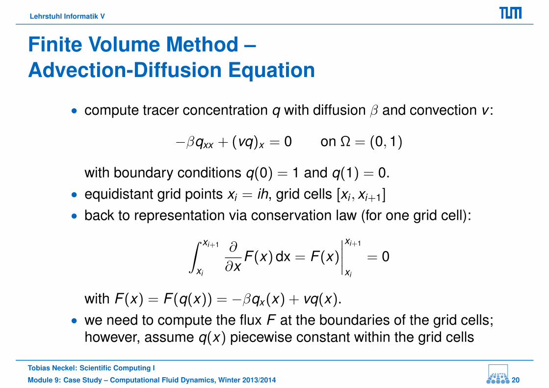
• compute tracer concentration q with diffusion β and convection v :
−βqxx + (vq)x = 0 on Ω = (0,1)
with boundary conditions q(0) = 1 and q(1) = 0.• equidistant grid points xi = ih, grid cells [xi , xi+1]
• back to representation via conservation law (for one grid cell):∫ xi+1
xi
∂
∂xF (x) dx = F (x)
∣∣∣∣xi+1
xi
= 0
with F (x) = F (q(x)) = −βqx (x) + vq(x).• we need to compute the flux F at the boundaries of the grid cells;
however, assume q(x) piecewise constant within the grid cells
Tobias Neckel: Scientific Computing I
Module 9: Case Study – Computational Fluid Dynamics, Winter 2013/2014 20

Lehrstuhl Informatik V
Finite Volume Method –Advection-Diffusion Equation (2)
• wanted: compute F (xi ) with F (q(x)) = −βqx (x) + vq(x)• where q(x) := qi for each Ωi = [xi , xi+1]• computing the diffusive flux is straightforward:
−βqx∣∣xi+1
= −β q(xi+1)− q(xi )
h• options for advective flux vq:
• symmetric flux:
vq∣∣xi+1
=vq(xi ) + vq(xi+1)
2• “upwind” flux:
vq∣∣xi+1
=
vq(xi ) if v > 0vq(xi+1) if v < 0
Tobias Neckel: Scientific Computing I
Module 9: Case Study – Computational Fluid Dynamics, Winter 2013/2014 21

Lehrstuhl Informatik V
Finite Volume Method –Advection-Diffusion Equation (3)
• system of equations: for all i
F (x)
∣∣∣∣xi+1
xi
= F (xi+1)− F (xi ) = 0
• for symmetric flux:
−β q(xi+1)− 2q(xi ) + q(xi−1)
h2 + vq(xi+1)− q(xi−1)
2h= 0
leads to non-physical behaviour as soon as β < vh2
(observe signs of matrix elements!)• system of equations for upwind flux (assume v > 0):
−β q(xi+1)− 2q(xi ) + q(xi−1)
h2 + vq(xi )− q(xi−1)
h= 0
→ stable, but overly diffusive solutions (positive definite matrix)
Tobias Neckel: Scientific Computing I
Module 9: Case Study – Computational Fluid Dynamics, Winter 2013/2014 22

Lehrstuhl Informatik V
Marker-and-Cell Method – Staggered Grid
Marker-and-Cell method (Harlow and Welch, 1965):• discretization scheme: Finite Differences• can be shown to be equivalent to Finite Volumes, however• based on a so-called staggered grid:
• Cartesian grid (rectangular grid cells),with cell centres at xi,j := (ih, jh), e.g.
• pressure located in cell centres• velocities (those in normal direction) located on cell edges
Tobias Neckel: Scientific Computing I
Module 9: Case Study – Computational Fluid Dynamics, Winter 2013/2014 23
Lehrstuhl Informatik V
Spatial Discretisation – Continuity Equation:
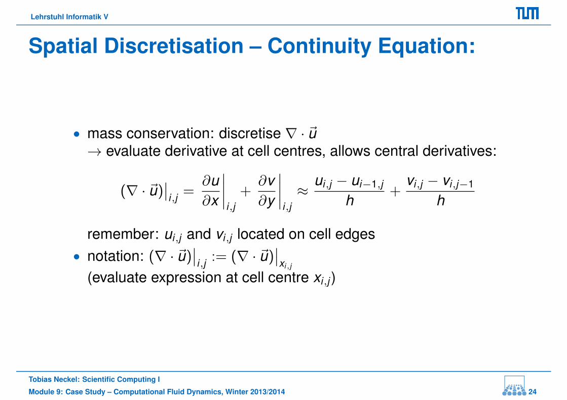
• mass conservation: discretise ∇ · ~u→ evaluate derivative at cell centres, allows central derivatives:
(∇ · ~u)∣∣i,j =
∂u∂x
∣∣∣∣i,j
+∂v∂y
∣∣∣∣i,j≈ ui,j − ui−1,j
h+
vi,j − vi,j−1
h
remember: ui,j and vi,j located on cell edges• notation: (∇ · ~u)
∣∣i,j := (∇ · ~u)
∣∣xi,j
(evaluate expression at cell centre xi,j )
Tobias Neckel: Scientific Computing I
Module 9: Case Study – Computational Fluid Dynamics, Winter 2013/2014 24

Lehrstuhl Informatik V
Spatial Discretisation – Pressure Terms
• note: velocities located on midpoints of cell edges
∂u∂t
∣∣∣∣i+ 1
2 ,j= . . . ,
∂v∂t
∣∣∣∣i,j+ 1
2
= . . .
=⇒ all derivatives need to be approximated at midpoints of celledges!
• pressure term ∇p: central differences for first derivatives(as pressure is located in cell centres)
∂p∂x
∣∣∣∣i+ 1
2 ,j≈ pi+1,j − pi,j
h,
∂p∂y
∣∣∣∣i,j+ 1
2
≈ pi,j+1 − pi,j
h
Tobias Neckel: Scientific Computing I
Module 9: Case Study – Computational Fluid Dynamics, Winter 2013/2014 25

Lehrstuhl Informatik V
Spatial Discretisation – Diffusion Term
• for diffusion term ∆~u: use standard 5- or 7-point stencil• 2D:
∆u∣∣i,j ≈
ui−1,j + ui,j−1 − 4ui,j + ui+1,j + ui,j+1
h2
• 3D:
∆u∣∣i,j,k ≈
ui−1,j,k + ui,j−1,k + ui,j,k−1 − 6ui,j,k + ui+1,j,k + ui,j+1,k + ui,j,k+1
h2
Tobias Neckel: Scientific Computing I
Module 9: Case Study – Computational Fluid Dynamics, Winter 2013/2014 26

Lehrstuhl Informatik V
Spatial Discretisation – Convection Terms
• treat derivatives of nonlinear terms (~u · ∇)~u:• central differences (for momentum equation in x-direction):
u∂u∂x
∣∣∣∣i+ 1
2 ,j≈ ui,j
ui+1,j − ui−1,j
2h, v
∂u∂y
∣∣∣∣i+ 1
2 ,j≈ v
∣∣xi+ 1
2 ,j
ui,j+1 − ui,j−1
2h
with v∣∣xi+ 1
2 ,j= 1
4
(vi,j + vi,j−1 + vi+1,j + vi+1,j−1
)
• upwind differences (for momentum equation in x-direction):
u∂u∂x
∣∣∣∣xi+ 1
2 ,j
≈ ui,jui,j − ui−1,j
2h, v
∂u∂y
∣∣∣∣xi+ 1
2 ,j
≈ v∣∣xi+ 1
2 ,j
ui,j − ui,j−1
2h
if ui,j > 0 and v∣∣xi+ 1
2 ,j> 0
• mix of central and upwind differences possible and used
Tobias Neckel: Scientific Computing I
Module 9: Case Study – Computational Fluid Dynamics, Winter 2013/2014 27

Lehrstuhl Informatik V
Time Discretisation
• recall the incompressible Navier-Stokes equations:
∇ · ~u = 0∂
∂t~u + (~u · ∇)~u = −∇p +
1Re
∆~u + f
• note the role of the unknowns:→ 2 or 3 equations for velocities (x , y , and z component)
resulting from momentum conservation→ 4th equation (mass conservation) to “ close” the system;
required to determine pressure p→ however, p does not occur explicitly in mass conservation
• possible approach: Chorin’s projection method→ p acts as a variable to enforce the mass conservation as
“side condition”
Tobias Neckel: Scientific Computing I
Module 9: Case Study – Computational Fluid Dynamics, Winter 2013/2014 28
Lehrstuhl Informatik V
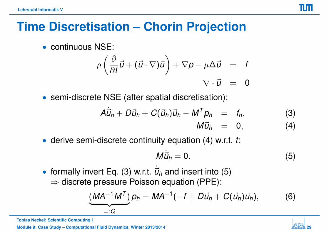
Time Discretisation – Chorin Projection• continuous NSE:
ρ
(∂
∂t~u + (~u · ∇)~u
)+∇p − µ∆~u = f
∇ · ~u = 0
• semi-discrete NSE (after spatial discretisation):
A~uh + D~uh + C(~uh)~uh −MT ph = fh, (3)M~uh = 0, (4)
• derive semi-discrete continuity equation (4) w.r.t. t :
M~uh = 0. (5)
• formally invert Eq. (3) w.r.t. ~uh and insert into (5)⇒ discrete pressure Poisson equation (PPE):
(MA−1MT )︸ ︷︷ ︸=:Q
ph = MA−1(−f + D~uh + C(~uh)~uh), (6)
Tobias Neckel: Scientific Computing I
Module 9: Case Study – Computational Fluid Dynamics, Winter 2013/2014 29

Lehrstuhl Informatik V
Time Discretisation – Chorin Projection
• updating the velocities:• discretise time with explicit method (explicit Euler, e.g.):
~u(n+1)h − ~u(n)
hτ
= . . .
• update velocity “correctly”: solve momentum equations (3)• use pressure ph of PPE solution to compute discrete
pressure gradients MT ph:
⇒ ~u(n+1)h = ~u(n)
h + τ(−D~u(n)
h − C(~u(n)h )~u(n)
h +~f (n)h + MT ph
)
• costs: solve 1 linear system of equations in each time step!
Tobias Neckel: Scientific Computing I
Module 9: Case Study – Computational Fluid Dynamics, Winter 2013/2014 30

Lehrstuhl Informatik V
Implementation
• geometry representation as a flag field (Marker-and-Cell)
flag field as an array of booleans:0 0 0 0 0 0 0 0 0 0 0 0 0 0 0 0 0 0 0 0 0 0 0 00 0 0 0 0 0 0 0 0 0 0 0 0 0 0 0 0 0 0 0 0 0 0 00 0 0 0 0 0 0 0 1 1 0 0 0 0 0 0 0 0 0 0 0 0 0 00 0 0 0 0 0 0 0 0 1 1 0 0 0 0 0 0 0 0 0 0 0 0 00 0 0 0 0 0 0 0 0 0 1 1 0 0 0 0 0 0 0 0 0 0 0 00 0 0 0 0 0 0 0 0 0 0 1 1 0 0 0 0 0 0 0 0 0 0 00 0 0 0 0 0 0 0 0 0 0 0 0 0 0 0 0 0 0 0 0 0 0 00 0 0 0 0 0 0 0 0 0 0 0 0 0 0 0 0 0 0 0 0 0 0 0
• input data (boundary conditions) and output data (computedresults) as arrays
Tobias Neckel: Scientific Computing I
Module 9: Case Study – Computational Fluid Dynamics, Winter 2013/2014 31

Lehrstuhl Informatik V
Implementation (2)
Lab course “Scientific Computing – Computational Fluid Dynamics”:• modular C/C++ code• parallelization:
• simple data parallelism, domain decomposition• straightforward MPI-based parallelization (exchange of
ghost layers)• target architectures:
• parallel computers with distributed memory• clusters
• possible extensions:• free-surface flows (“the falling drop”)• multigrid solver for the pressure equation• heat transfer
Tobias Neckel: Scientific Computing I
Module 9: Case Study – Computational Fluid Dynamics, Winter 2013/2014 32

Lehrstuhl Informatik V
Part III: The Shallow Water Equations and FiniteVolumes Revisited
The Shallow Water EquationsModelling Scenario: Tsunami Simulation
Finite Volume DiscretisationCentral and Upwind FluxesLax-Friedrichs Flux
Towards Tsunami SimulationWave Speed of TsunamisTreatment of Bathymetry Data
Tobias Neckel: Scientific Computing I
Module 9: Case Study – Computational Fluid Dynamics, Winter 2013/2014 33

Lehrstuhl Informatik V
The Shallow Water Equations
∂
∂t
hhuhv
+
∂
∂x
huhu2 + 1
2 gh2
huv
+
∂
∂y
hvhuv
hv2 + 12 gh2
= S(t , x , y)
Comments on modelling:• generalized 2D hyperbolic PDE: q = (h,hu,hv)T
∂
∂tq +
∂
∂xF (q) +
∂
∂yG(q) = S(t , x , y)
derived from conservations laws for mass and momentum• may be derived by vertical averaging from the 3D incompressible
Navier-Stokes equations• compare to Euler equations: density ρ vs. water depth h
Tobias Neckel: Scientific Computing I
Module 9: Case Study – Computational Fluid Dynamics, Winter 2013/2014 34

Lehrstuhl Informatik V
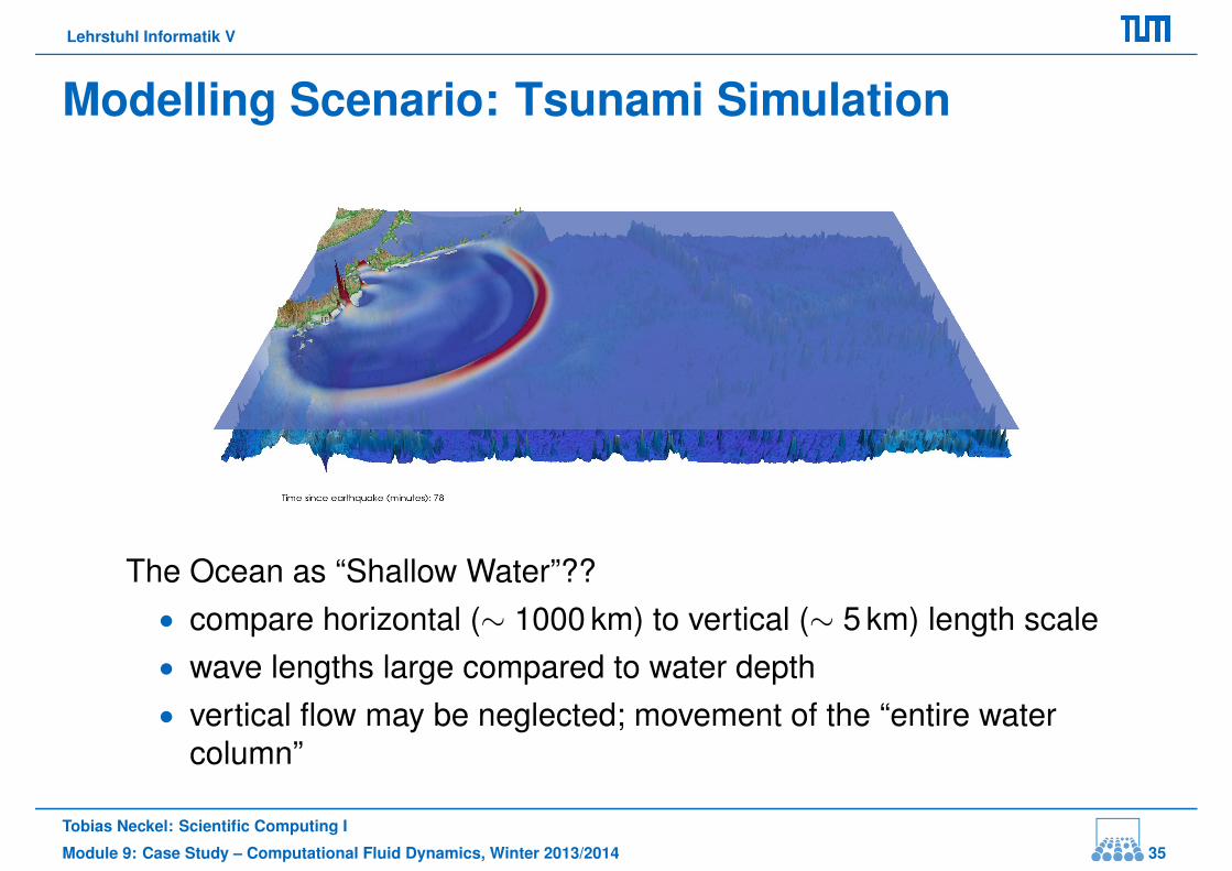
Modelling Scenario: Tsunami Simulation
The Ocean as “Shallow Water”??• compare horizontal (∼ 1000 km) to vertical (∼ 5 km) length scale• wave lengths large compared to water depth• vertical flow may be neglected; movement of the “entire water
column”
Tobias Neckel: Scientific Computing I
Module 9: Case Study – Computational Fluid Dynamics, Winter 2013/2014 35

Lehrstuhl Informatik V
Modelling Scenario: Tsunami Simulation
The Ocean as “Shallow Water”??• compare horizontal (∼ 1000 km) to vertical (∼ 5 km) length scale• wave lengths large compared to water depth• vertical flow may be neglected; movement of the “entire water
column”
Tobias Neckel: Scientific Computing I
Module 9: Case Study – Computational Fluid Dynamics, Winter 2013/2014 35

Lehrstuhl Informatik V
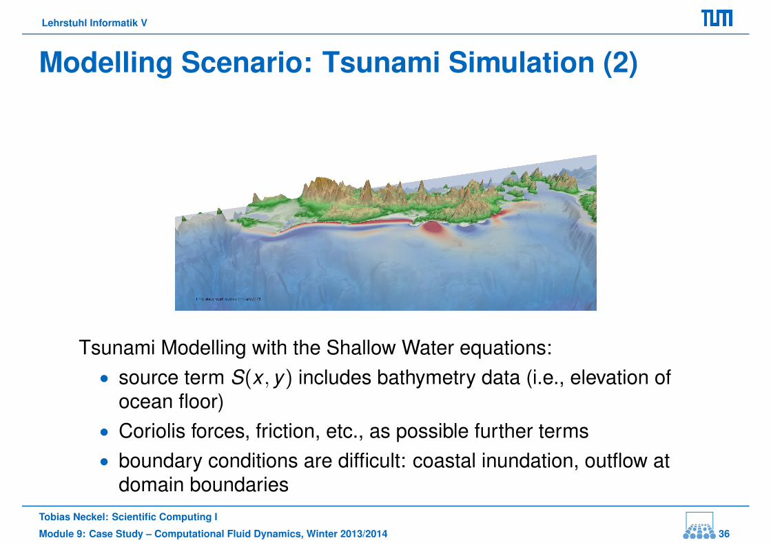
Modelling Scenario: Tsunami Simulation (2)
Tsunami Modelling with the Shallow Water equations:• source term S(x , y) includes bathymetry data (i.e., elevation of
ocean floor)• Coriolis forces, friction, etc., as possible further terms• boundary conditions are difficult: coastal inundation, outflow at
domain boundariesTobias Neckel: Scientific Computing I
Module 9: Case Study – Computational Fluid Dynamics, Winter 2013/2014 36
Lehrstuhl Informatik V
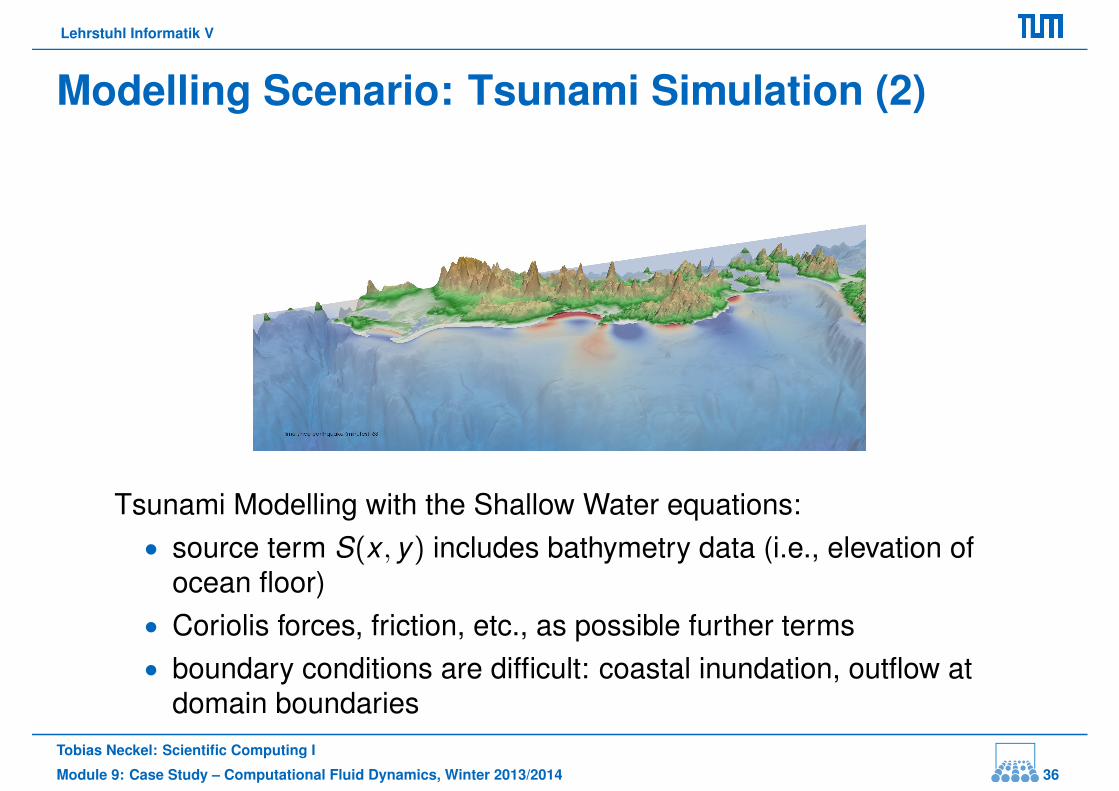
Modelling Scenario: Tsunami Simulation (2)
Tsunami Modelling with the Shallow Water equations:• source term S(x , y) includes bathymetry data (i.e., elevation of
ocean floor)• Coriolis forces, friction, etc., as possible further terms• boundary conditions are difficult: coastal inundation, outflow at
domain boundariesTobias Neckel: Scientific Computing I
Module 9: Case Study – Computational Fluid Dynamics, Winter 2013/2014 36
Lehrstuhl Informatik V
Modelling Scenario: Tsunami Simulation (2)
Tsunami Modelling with the Shallow Water equations:• source term S(x , y) includes bathymetry data (i.e., elevation of
ocean floor)• Coriolis forces, friction, etc., as possible further terms• boundary conditions are difficult: coastal inundation, outflow at
domain boundariesTobias Neckel: Scientific Computing I
Module 9: Case Study – Computational Fluid Dynamics, Winter 2013/2014 36

Lehrstuhl Informatik V
Finite Volume Discretisation
• discretise system of PDEs
∂
∂tq +
∂
∂xF (q) +
∂
∂yG(q) = S(t , x , y)
• with
q :=
hhuhv
F (q) :=
huhu2 + 1
2 gh2
huv
G(q) :=
hvhuv
hv2 + 12 gh2
• basic form of numerical schemes:
Q(n+1)i,j = Q(n)
i,j −τ
h
(F (n)
i+ 12 ,j− F (n)
i− 12 ,j
)− τ
h
(G(n)
i,j+ 12−G(n)
i,j− 12
)
where F (n)i+ 1
2 ,j, G(n)
i,j+ 12, . . . approximate the flux functions F (q) and
G(q) at the grid cell boundaries
Tobias Neckel: Scientific Computing I
Module 9: Case Study – Computational Fluid Dynamics, Winter 2013/2014 37
Lehrstuhl Informatik V
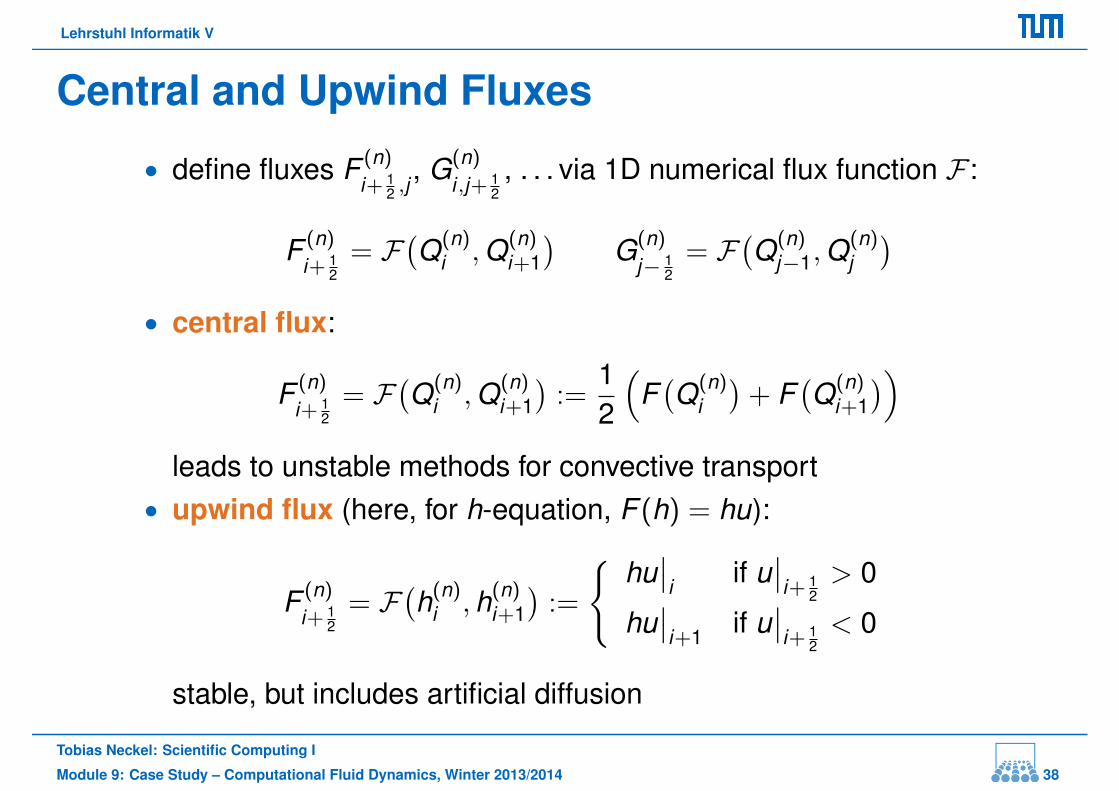
Central and Upwind Fluxes
• define fluxes F (n)i+ 1
2 ,j, G(n)
i,j+ 12, . . . via 1D numerical flux function F :
F (n)i+ 1
2= F
(Q(n)
i ,Q(n)i+1
)G(n)
j− 12
= F(Q(n)
j−1,Q(n)j
)
• central flux:
F (n)i+ 1
2= F
(Q(n)
i ,Q(n)i+1
):=
12
(F(Q(n)
i
)+ F
(Q(n)
i+1
))
leads to unstable methods for convective transport• upwind flux (here, for h-equation, F (h) = hu):
F (n)i+ 1
2= F
(h(n)
i ,h(n)i+1
):=
hu∣∣i if u
∣∣i+ 1
2> 0
hu∣∣i+1 if u
∣∣i+ 1
2< 0
stable, but includes artificial diffusion
Tobias Neckel: Scientific Computing I
Module 9: Case Study – Computational Fluid Dynamics, Winter 2013/2014 38

Lehrstuhl Informatik V
(Local) Lax-Friedrichs Flux
• classical Lax-Friedrichs method uses as numerical flux:
F (n)i+ 1
2= F
(Q(n)
i ,Q(n)i+1
):=
12
(F(Q(n)
i
)+ F
(Q(n)
i+1
))− h
2τ(Q(n)
i+1−Q(n)i
)
• can be interpreted as central flux plus diffusion flux:
h2τ(Q(n)
i+1 −Q(n)i
)=
h2
2τ·
Q(n)i+1 −Q(n)
i
h
with diffusion coefficient h2
2τ , where c := hτ is some kind of
velocity (“one grid cell per time step”)• idea of local Lax-Friedrichs method: use the “appropriate”
velocity
F (n)i+ 1
2:=
12
(F(Q(n)
i
)+ F
(Q(n)
i+1
))−
ai+ 12
2(Q(n)
i+1 −Q(n)i
)
Tobias Neckel: Scientific Computing I
Module 9: Case Study – Computational Fluid Dynamics, Winter 2013/2014 39
Lehrstuhl Informatik V
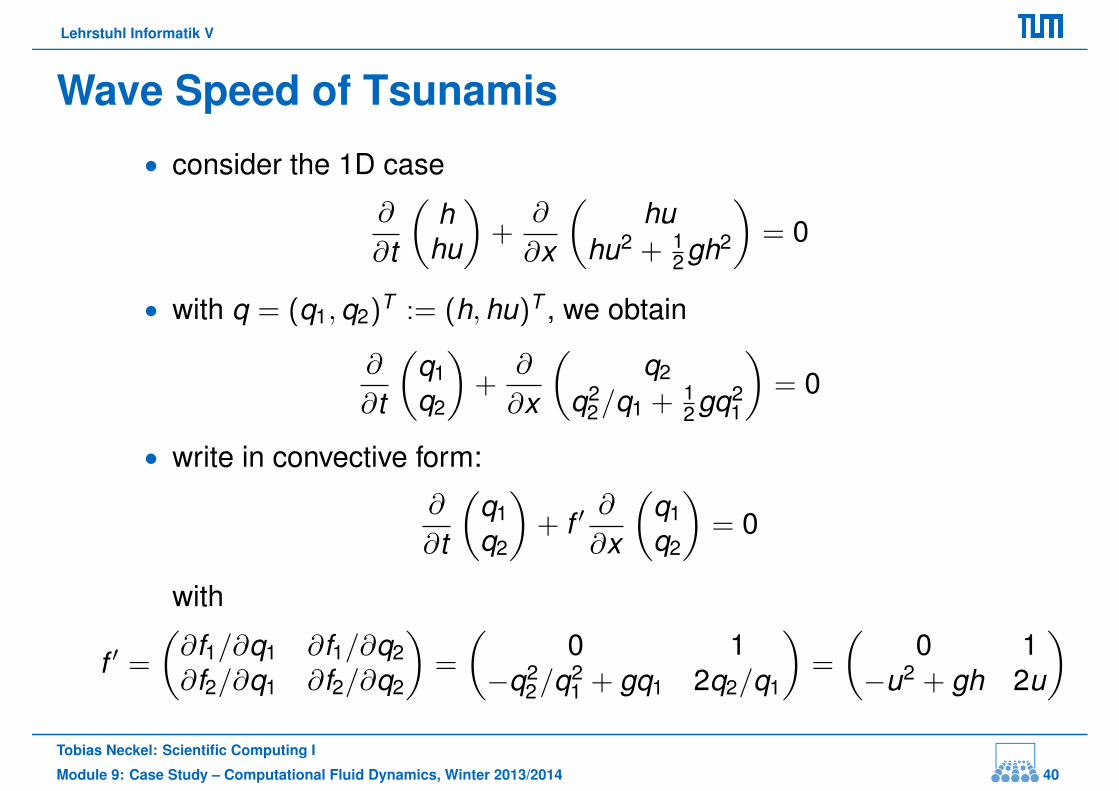
Wave Speed of Tsunamis
• consider the 1D case
∂
∂t
(h
hu
)+
∂
∂x
(hu
hu2 + 12 gh2
)= 0
• with q = (q1,q2)T := (h,hu)T , we obtain
∂
∂t
(q1q2
)+
∂
∂x
(q2
q22/q1 + 1
2 gq21
)= 0
• write in convective form:
∂
∂t
(q1q2
)+ f ′
∂
∂x
(q1q2
)= 0
with
f ′ =
(∂f1/∂q1 ∂f1/∂q2∂f2/∂q1 ∂f2/∂q2
)=
(0 1
−q22/q
21 + gq1 2q2/q1
)=
(0 1
−u2 + gh 2u
)
Tobias Neckel: Scientific Computing I
Module 9: Case Study – Computational Fluid Dynamics, Winter 2013/2014 40
Lehrstuhl Informatik V
Wave Speed of Tsunamis (2)
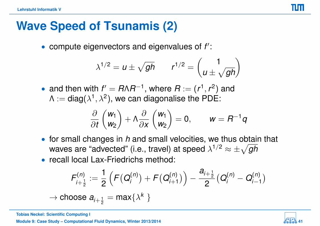
• compute eigenvectors and eigenvalues of f ′:
λ1/2 = u ±√
gh r1/2 =
(1
u ±√
gh
)
• and then with f ′ = RΛR−1, where R := (r1, r2) andΛ := diag(λ1, λ2), we can diagonalise the PDE:
∂
∂t
(w1w2
)+ Λ
∂
∂x
(w1w2
)= 0, w = R−1q
• for small changes in h and small velocities, we thus obtain thatwaves are “advected” (i.e., travel) at speed λ1/2 ≈ ±
√gh
• recall local Lax-Friedrichs method:
F (n)i+ 1
2:=
12
(F(Q(n)
i
)+ F
(Q(n)
i+1
))−
ai+ 12
2(Q(n)
i −Q(n)i−1
)
→ choose ai+ 12
= maxλk Tobias Neckel: Scientific Computing I
Module 9: Case Study – Computational Fluid Dynamics, Winter 2013/2014 41

Lehrstuhl Informatik V
Shallow Water Equations with Bathymetry
h
b
∂
∂t
hhuhv
+
∂
∂x
huhu2 + 1
2 gh2
huv
+
∂
∂y
hvhuv
hv2 + 12 gh2
=
0−(ghb)x−(ghb)y
Questions for numerics:• treat (bh)x and (bh)y as source terms or include these into flux
computations?• preserve certain properties of solutions – e.g., “lake at rest”
Tobias Neckel: Scientific Computing I
Module 9: Case Study – Computational Fluid Dynamics, Winter 2013/2014 42
Lehrstuhl Informatik V
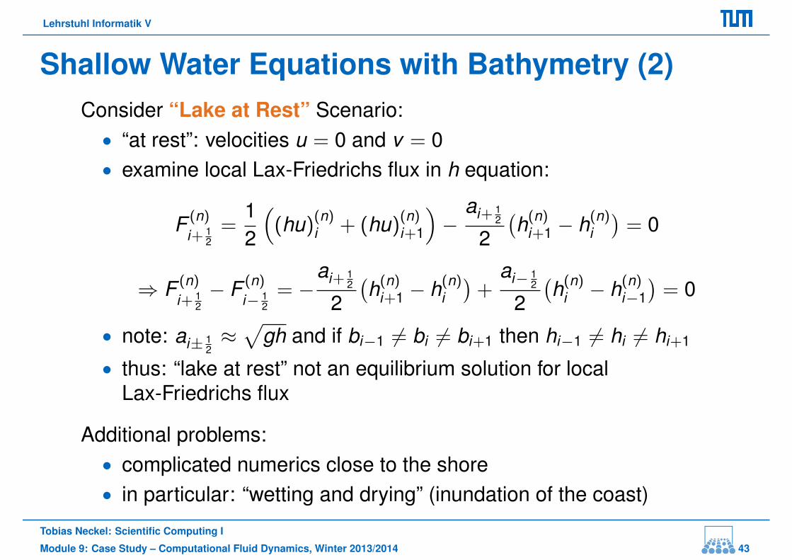
Shallow Water Equations with Bathymetry (2)Consider “Lake at Rest” Scenario:
• “at rest”: velocities u = 0 and v = 0• examine local Lax-Friedrichs flux in h equation:
F (n)i+ 1
2=
12
((hu)
(n)i + (hu)
(n)i+1
)−
ai+ 12
2(h(n)
i+1 − h(n)i
)= 0
⇒ F (n)i+ 1
2− F (n)
i− 12
= −ai+ 1
2
2(h(n)
i+1 − h(n)i
)+
ai− 12
2(h(n)
i − h(n)i−1
)= 0
• note: ai± 12≈√
gh and if bi−1 6= bi 6= bi+1 then hi−1 6= hi 6= hi+1
• thus: “lake at rest” not an equilibrium solution for localLax-Friedrichs flux
Additional problems:• complicated numerics close to the shore• in particular: “wetting and drying” (inundation of the coast)
Tobias Neckel: Scientific Computing I
Module 9: Case Study – Computational Fluid Dynamics, Winter 2013/2014 43

Lehrstuhl Informatik V
References and Literature
Course material is mostly based on:• R. J. LeVeque: Finite Volume Methods for Hyperbolic Equations,
Cambridge Texts in Applied Mathematics, 2002.• M. Griebel, T. Dornseifer and T. Neunhoeffer: Numerical
Simulation in Fluid Dynamics: A Practical Introduction,SIAM Monographs on Mathematical Modeling and Computation,SIAM, 1997.
Shallow Water Code SWE:→ http://www5.in.tum.de/SWE/
Tobias Neckel: Scientific Computing I
Module 9: Case Study – Computational Fluid Dynamics, Winter 2013/2014 44