Efï¬cient Discretisation for Link Travel Time Models

Networks and Spatial Economics, 4: (2004) 269–290©C 2004 Kluwer Academic Publishers, Manufactured in the Netherlands.

Efficient Discretisation for Link Travel Time Models

MALACHY CAREY∗Y.E. GESchool of Management and Economics, Queen’s University Belfast, Northern Ireland, BT7 1NNemail: [email protected]: [email protected]

Abstract

In the literature, two different models have been used to compute link travel times in dynamic traffic assignment(DTA), and elsewhere we investigated how these are affected by discretising the link length. Here we considerdiscretising time as well as space (the link length). We vary the discretising of time with spatial discretisation heldfixed, and vice versa, and also vary both together. The results show that “coordinated” discretisation is usually themost efficient in approximating the limit solution (continuous time, continuous space) and, even when it is not themost efficient, it has other advantages. The results have implications for algorithms for DTA and for the choiceof discrete versus continuous time models. For example, refining the discretisation of time (without refining itfor space) can make the solution less accurate, so that in the widely used whole-link models (i.e. without spatialdiscretisation) it is more efficient to use the largest feasible time steps, close to the link travel time.

Keywords: Dynamic traffic assignment, link travel times, road traffic networks, efficient discretisation

1. Introduction

Dynamic traffic assignment (DTA) concerns the determination of traffic loadings (num-bers of vehicles per unit time) and travel times on links and paths of a road network whenthese are varying over time. We consider DTA models that use link travel-time functions.We note that these DTA models can be classified as continuous time or discrete time andthere is usually a continuous time and discrete time version of any DTA model (e.g., Wuet al., 1998). It appears to be widely accepted that the continuous time formulation is morerealistic and more accurate. The discrete time formulation is often introduced as a neces-sary or convenient device to obtain approximate numerical solutions to the continuous timeformulation, and for a best approximation it is assumed or recommended that the lengthsof time intervals should be as small as possible. Using such small time steps is compu-tationally costly for medium or large traffic networks. In this paper we consider whethersuch small time steps really give us more realistic solutions. We use the solutions from thewell-known Lighthill, Whitham, Richards (LWR) model (Lighthill and Whitham, 1955;Richards, 1956) as a benchmark for comparisons, but nevertheless, the paper is intended asa contribution to investigating DTA models for networks, and not a contribution to traffic flowtheory.

∗To whom all correspondence should be addressed.

270 CAREY AND GE

It turns out that the closeness to the LWR solution depends on the discretisation of space(the link length) as well as time, hence we consider discretising both and ask what is the bestcombination of time and space step sizes. We consider both the quality of the solution andthe computing cost. An algorithm, or a discretisation scheme, is said to be more efficient ifit yields the same accuracy (or quality of solution) for a smaller computing cost, or a greateraccuracy (or quality of solution) for the same computing cost. To focus the discussion weconsider a single link with various profiles of inflows and assume link travel-time functionsfrom the DTA literature.

Travel time on a link, in the existing DTA literature, is generally treated as a function ofvariables related to the whole link. A model widely used in DTA is τ (t) = f (x(t)), whereτ (t) is the link travel time for vehicles entering a link at time t , and x(t) is the number ofvehicles on the link at time t . The properties of models of this kind have been investigatedextensively by Friesz et al. (1993), Astarita (1995, 1996), Wu et al. (1995, 1998), Ranet al. (1997), Xu et al. (1999), Carey and McCartney (2002), Zhu and Marcotte (2000), andAdamo et al. (1999). More recently Carey et al. (2003) introduced an alternative travel-timemodel, τ (t) = h(w(t)), in which the travel time τ (t) for a user entering the link at time tis taken as a function of the average flow rate w(t) over the link during the time period atraveler entering at time t traverses the link.

In Carey and Ge (2001, 2003) it is shown that if one treats time as continuous and divides ahomogeneous link, without obstructions, into shorter segments then as the segment lengthsapproach zero the solution profiles, for say outflow and travel time, from the above twowhole-link models converge to the solution from the LWR model. Hence, when comparingsolutions from various discretisation schemes, we use the solution from the LWR modelas the benchmark. Of course, to make the travel-time models comparable with the LWRmodel we use functional form of the former that is consistent with the latter and vice versa.In the next section we set out the travel-time models used.

These travel-time models are normally applied to whole links in network models for DTA,without discretising the link length. However, in Section 3 we consider various combinationsof discretisation(step sizes) for time and space, varying the discretisation of one whileholding the other fixed and vice versa. From these experiments we show that the mostefficient discretisation is obtained by choosing the minimum number of time steps for anygiven discretisation of space, which we refer to as ‘coordinated’ discretisation. We illustratethis for various inflow patterns and functional forms of travel-time functions. The resultshave obvious implications for discretisation schemes used in network models for DTA.

2. Link travel-time models to be investigated

This section sets out particular functional forms that will be used in later numerical examples,for the travel-time models τ = f (x) and τ = h(w), and the flow density function q = Q(k)used in the LWR model. We choose linear and quadratic forms of τ = f (x) and derive thecorresponding functional forms of τ = h(w) and q = Q(k). To derive the latter we notethat all three forms should yield the same solution when the link flow, density and speedon the link, or link segment, are assumed to be constant. In that case, x = τq and x = Lk,where x is the number of vehicles on the link, τ is the link travel time, q is the link flow rate,

EFFICIENT DISCRETISATION FOR LINK TRAVEL TIME MODELS 271

k is the link density and L is the link length. We use these to derive comparable functionalforms.

Using a linear form of τ = f (x). The earliest form of τ = f (x) used in DTA (Frieszet al., 1993) was the linear form, which can be stated as

τ = a + bx (1)

where a and b can be interpreted to be the free-flow travel time and the minimum headway onthe link of interest, respectively. To obtain the corresponding form of τ = h(w), substitutingx = τq into Eq. (1) and letting w = q and rearranging gives

τ = a/(1 − bw) (2)

To obtain the corresponding flow-density relationship, for the associated LWR model, sub-stitute x = Lk and τ = x/q = Lk/q in (1), and rearrange, thus

q = Lk/(a + bLk) (3)

Using a quadratic form of τ = f (x). A quadratic travel-time function is used in Wuet al. (1998) and Xu et al. (1999) and can be written as

τ = a + bx + cx2 (4)

where a and b have the same interpretation as in model (1), and c is a parameter to becalibrated and its physical meaning is discussed in Carey and Ge (2001). As above, wederive the model of τ = h(w) as

τ = a + bqτ + cq2τ 2 (5)

or

τ = (1 − bq) ±√

(1 − bq)2 − 4acq2

2cq2(6)

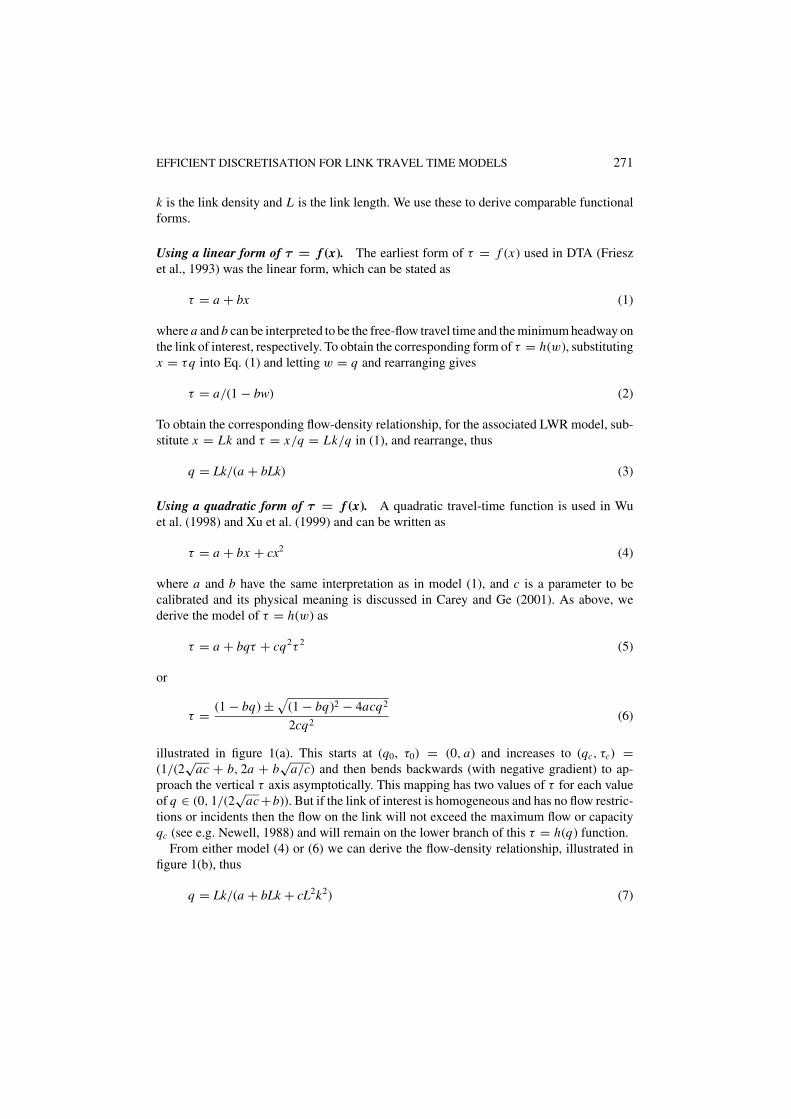
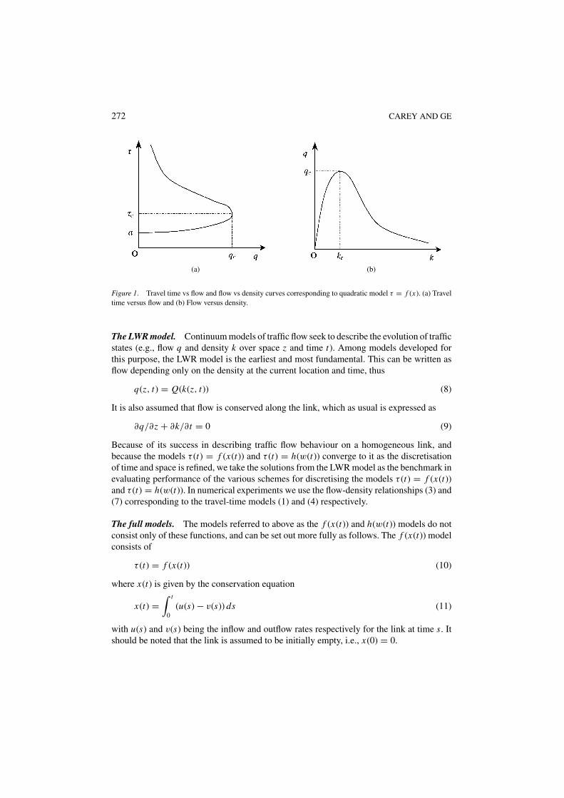
illustrated in figure 1(a). This starts at (q0, τ0) = (0, a) and increases to (qc, τc) =(1/(2

√ac + b, 2a + b

√a/c) and then bends backwards (with negative gradient) to ap-

proach the vertical τ axis asymptotically. This mapping has two values of τ for each valueof q ∈ (0, 1/(2

√ac+b)). But if the link of interest is homogeneous and has no flow restric-

tions or incidents then the flow on the link will not exceed the maximum flow or capacityqc (see e.g. Newell, 1988) and will remain on the lower branch of this τ = h(q) function.

From either model (4) or (6) we can derive the flow-density relationship, illustrated infigure 1(b), thus

q = Lk/(a + bLk + cL2k2) (7)

272 CAREY AND GE

(a) (b)

Figure 1. Travel time vs flow and flow vs density curves corresponding to quadratic model τ = f (x). (a) Traveltime versus flow and (b) Flow versus density.

The LWR model. Continuum models of traffic flow seek to describe the evolution of trafficstates (e.g., flow q and density k over space z and time t). Among models developed forthis purpose, the LWR model is the earliest and most fundamental. This can be written asflow depending only on the density at the current location and time, thus

q(z, t) = Q(k(z, t)) (8)

It is also assumed that flow is conserved along the link, which as usual is expressed as

∂q/∂z + ∂k/∂t = 0 (9)

Because of its success in describing traffic flow behaviour on a homogeneous link, andbecause the models τ (t) = f (x(t)) and τ (t) = h(w(t)) converge to it as the discretisationof time and space is refined, we take the solutions from the LWR model as the benchmark inevaluating performance of the various schemes for discretising the models τ (t) = f (x(t))and τ (t) = h(w(t)). In numerical experiments we use the flow-density relationships (3) and(7) corresponding to the travel-time models (1) and (4) respectively.

The full models. The models referred to above as the f (x(t)) and h(w(t)) models do notconsist only of these functions, and can be set out more fully as follows. The f (x(t)) modelconsists of

τ (t) = f (x(t)) (10)

where x(t) is given by the conservation equation

x(t) =∫ t

0(u(s) − v(s)) ds (11)

with u(s) and v(s) being the inflow and outflow rates respectively for the link at time s. Itshould be noted that the link is assumed to be initially empty, i.e., x(0) = 0.


In the h(w(t)) model (Carey et al., 2003)

τ (t) = h(w(t)) (12)

where w(t) is an estimate of the mean flow rate over the link during the period a vehicleentering at time t traverses the link. An estimate of the average flow rate can be taken as

w(t) = βu(t) + (1 − β)v(t + τ (t)), (13)

where β is a weighting constant 1 > β ≥ 0. To define the outflow rate v(t + τ (t)) they usethe flow propagation equation

v(t + τ (t)) = u(t)/[1 + τ ′(t)], (14)

Combining (12) to (14) the model can be written as

τ (t) = h

(βu(t) + (1 − β)

u(t)

1 + τ ′(t)

), (15)

Carey and Ge (2003) show that (14) also implies (11).In the rest of the paper when we refer to (10)–(11) as the f (x(t)) model and (12)–(14)

or (15) as the h(w(t)) model. For brevity we often abbreviate this to f (x) and h(w). Bysolving the f (x(t)) and h(w(t)) models we mean taking a given profile of inflows u(t) toa link over the time horizon [0, T ] and using the models to compute the profile of traveltimes and outflows from the link over the same time horizon.

2.1. Discretising the models

The models f (x(t)) and h(w(t)) are stated above for continuous time but in general, evenfor simple functional forms of f (·) and h(·), explicit analytical expressions for the solutionscan not be obtained. In view of that the models are usually solved by numerical methods,dividing time into small discrete intervals. Also, rather than applying the models directlyto the whole link, we here divide the link into segments and apply the models sequentiallyto these. A time-space discretised version of each model is set out in Carey and Ge (2001,2003) and it is not necessary to set that out again here. It is sufficient to note that the timehorizon [0, T ] is divided into equal intervals of length �t and the homogeneous link oflength L is divided into nL identical segments of length �x = L/nL . In the discretisedf (x) model the whole-link variable x(t) is replaced by variables xi j denoting the numberof vehicles on segment i at the beginning of time interval j . The whole-link inflows andoutflows u(t) and v(t) are replaced by ui j and vi j denoting the inflow and outflow raterespectively for link segment i in time interval j .

Feasible discretisation. We assume throughout that �t and �x are chosen so that the timestep �t is not greater than the time taken to traverse the link segment �x . If �t were largerthan that, it would introduce contradictions. In particular, it would imply that all traffic on�x at the start of any time interval �t would exit from �x before the end of the interval �t ,so that the segment would appear to be temporarily empty in the latter part of the interval�t .

274 CAREY AND GE

Setting �t less than or equal to the travel time for the link segment �x is not as simpleas it might seem. The problem is, the time taken to traverse the link, and hence to traversesegments of the link, can vary over time and is not known in advance. The discretisation�t and �x have to be chosen in advance of knowing the travel time on the link. However,we can ensure the above condition (�t not greater than the travel time on �x) by assuminga stronger condition,

�t ≤ the free-flow travel time (fftt) on �x . (16)

Let, nT = number of time steps into which the link fftt is divided, i.e. nT = (link fftt)/�t .Recall that nL = L/�x . Substituting �t = (link fftt)/nT and �x = L/nL into (16)

gives (link fftt)/nT ≤ link fftt/ nL hence (16) is equivalent to

nT ≥ nL . (17)

Suppose it is known in advance that, over the time horizon being considered, the traveltime on the link will never be less than some constant, say t∗, where t∗ is greater than thelink fftt. In that case the condition (16) could be replaced by �t ≤ (minimum travel timeon �x) = t1(�x/L), so that nT > nL . However, when applying the model to the linksof a network of even medium size, it is likely that on some links at some times the traveltime will be the fftt, hence these links will determine the �t and �x and will require thecondition (16). In view of that we will assume (16) rather than a weaker condition.

Definition. We refer to discretisation as coordinated if (16), or equivalently (17), is satisfiedas a strict equality, that is, if �t equals the free-flow travel time (fftt) on �x , or equivalentlynT = nL .

Since we have assumed a homogenous link, the segments �x are identical hence coordinateddiscretisation implies �t/(link fftt) = �x/L .

2.2. Measures of closeness of solution profiles over time

Later when we compute the solutions from f (x(t)) and h(w(t)) models we wish to comparethese solution profiles with those obtained using the LWR model. To measure the differencebetween the solution profiles we compute the percentage difference between them at a setof points in time, S = {t1, t2, . . . , t j , . . . }, over the time horizon [0, T ] and take the averageof these differences, to obtain the mean percentage difference, thus

MPDv = 100

|S||S|∑j=1

|vm(t j ) − v∗(t j )|v∗(t j )

(18)

where vm(t j ) is the outflow computed from the whole-link model τ (t) = f (x(t)) or τ (t) =h(w(t)) at time interval t j using m time intervals, v ∗ (t j ) is the outflow at time t j computedusing the LWR model, and |S| is the number of elements in the set S. To avoid a zerodenominator in (18) we exclude from S any t j for which v ∗ (t j ) is zero. (If desired we canalso exclude t j for which v ∗ (t j ) is close to zero.) The solutions of the f (x(t)) and h(w(t))


models are computed at m = T/�t points in time, hence we could compare with the LWRsolution at these points. However, for accuracy, we computed the solution of the LWR modelat a much larger number of points in time namely mL : in fact we used mL = 12,800. Wecan compute the solutions of the f (x(t)) and h(w(t)) models at these mL = 12,800 pointsin time by taking their solutions at the m points in time and linearly interpolating, which iswhat we did, so that we used |S| = 12,800. (In fact, any finer discretisation of time givesalmost the identical profiles of outflows and travel times from the LWR model.)

Similarly, the MPD for travel times is

MPDτ = 100

|S||S|∑j=1

|τm(t j ) − τ ∗(t j )|τ ∗(t j )

The mean percentage difference is a convenient simple measure, but such an average canobscure a wide range of values over the time horizon [0, T ]. We therefore also presentgraphs for some of the solutions (the link travel time and outflow profiles) over [0, T ] sothat these can be compared directly with each other.

3. Varying the pattern of discretisation, with a linear travel-time function f (x)

In this section we take the time-space discretised versions of the f (x(t)) and h(w(t)) models,apply these to a given profile of link inflows u(t) over the time horizon [0, T ], and computethe resulting solution profile for link travel times and link outflows over the same timehorizon. For brevity we refer to this as solving the f (x(t)) and h(w(t)) models. We examinehow the solutions vary as we vary the discretisation of time and space. The inflow profileis assumed to be

u(t) ={

(A + B) sin(π t/20) 0 ≤ t < 10

A + B sin5(π (t + 2)/24) 10 ≤ t < 22(19)

and is shown in each of the figures 2, 3 and 5 where A = 20 and B = 12. This inflow profileis continuously differentiable and starts from zero, i.e., u(0) = 0. The inflow profile waschosen with the peak inflow A + B = 32, as described in Carey and Ge (2001), to avoidsharp changes in the inflow rate. For f (x(t)) and h(w(t)) we used the forms (1) and (2), andsolved the models repeatedly for various time and space discretisations ranging from finestto roughest. The largest feasible link segments is �x = L and the smallest is �x = (segmentwith fftt equal to �t). This is equivalent to varying the number of segments nL from nL = 1to nL = nT . The largest feasible time step size is �t = (link fftt) and the smallest is �t =(arbitrarily small) which is effectively continuous time. This is equivalent to varying nT

from nT = 1 to nT = arbitrarily large. Typical results from these experiments are shown inTables 1 to 4 and figures 2, 3 and 5 and are discussed below. In previous papers, Carey andGe (2001, 2003) varied the discretisation of space while treating time as continuous. Thatis a special case of the scenarios in Section 3.1 below and corresponds to the final columnof Tables 1 to 4.

276 CAREY AND GE

(a) (b)

(c) (d)

Figure 2. Solutions from the f (x) and h(w) models, with nT fixed (nT = 8) and nL varying from nL = 1 tocoordinated (nL = nT ). (a) Outflow profiles for τ = f (x) model, (b) Outflow profiles for τ = h(w) model, (c)Travel time profiles for τ = f (x) model, and (d) Travel time profiles for τ = h(w) model.

3.1. Varying the space discretisation with the time discretisation held fixed

To discuss the effects of varying the discretisation of space and time we first consider refiningthe discretisation of space while holding the discretisation of time fixed. This correspondsto moving down the columns in Tables 1 to 4. The entries (MPDs) in all columns decreaseas we move down the column, which implies that, in all cases, refining the discretisationof space improves the solution (the approximation to the LWR solution) as measured byMPDv and MPDτ . (These results are also consistent with the results presented in Carey andGe (2001, 2003) which correspond to the final column in the tables.)

This is illustrated in more detail in figures 2(a)–(d) which correspond to a single column(column nT = 8) in Tables 1 to 4. Since there are some significant differences between theperformance of the f (x) and h(w) models, first consider the f (x) model. In figure 2(c), whenthe link is treated as a single segment (nL = 1) the link travel-time profile is significantlybelow the LWR profile, up to about 10% below. As �x decreases the travel-time profile


(a) (b)

(c) (d)

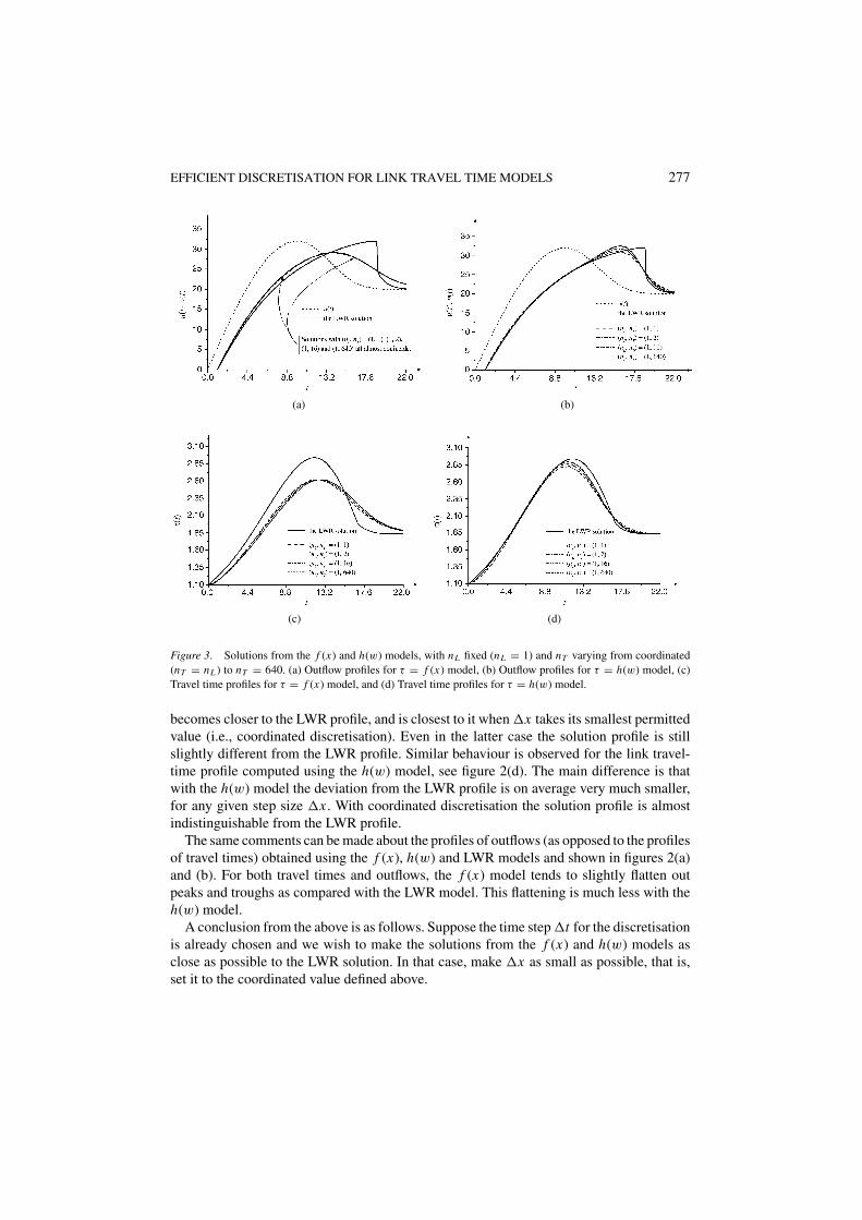
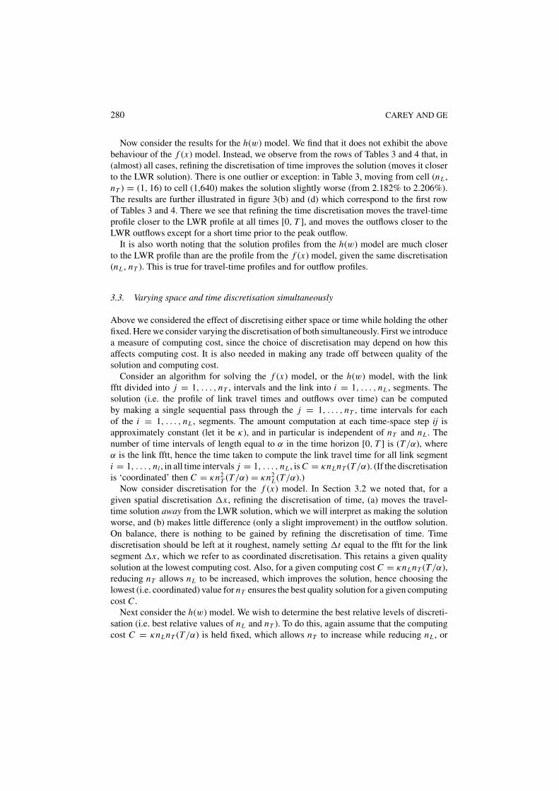
Figure 3. Solutions from the f (x) and h(w) models, with nL fixed (nL = 1) and nT varying from coordinated(nT = nL ) to nT = 640. (a) Outflow profiles for τ = f (x) model, (b) Outflow profiles for τ = h(w) model, (c)Travel time profiles for τ = f (x) model, and (d) Travel time profiles for τ = h(w) model.

becomes closer to the LWR profile, and is closest to it when �x takes its smallest permittedvalue (i.e., coordinated discretisation). Even in the latter case the solution profile is stillslightly different from the LWR profile. Similar behaviour is observed for the link travel-time profile computed using the h(w) model, see figure 2(d). The main difference is thatwith the h(w) model the deviation from the LWR profile is on average very much smaller,for any given step size �x . With coordinated discretisation the solution profile is almostindistinguishable from the LWR profile.

The same comments can be made about the profiles of outflows (as opposed to the profilesof travel times) obtained using the f (x), h(w) and LWR models and shown in figures 2(a)and (b). For both travel times and outflows, the f (x) model tends to slightly flatten outpeaks and troughs as compared with the LWR model. This flattening is much less with theh(w) model.

A conclusion from the above is as follows. Suppose the time step �t for the discretisationis already chosen and we wish to make the solutions from the f (x) and h(w) models asclose as possible to the LWR solution. In that case, make �x as small as possible, that is,set it to the coordinated value defined above.

278 CAREY AND GE

3.2. Varying the time discretisation with the space discretisation held fixed

Now consider the converse of the above, that is, consider refining the discretisation of timewhile holding the discretisation of space fixed. This corresponds to moving to the rightalong the rows of Tables 1 to 4. First consider the results for the f (x) model, in Tables 1and 2. We see that in all cases refining the discretisation of time very slightly improves theMPDv in Table 1. However, the improvement is very small (e.g., the largest change is in the

Table 1. MPDs of outflows for model τ = f (x).

Time

Space nT = 1 2 4 8 16 640

nL = 1 7.2666 7.1250 7.0738 7.0525 7.0441 7.0143

2 – 5.1238 4.9758 4.9206 4.8987 4.8631

4 – – 3.3543 3.2394 3.1969 3.1484

8 – – – 2.0431 1.9644 1.8964

16 – – – – 1.1764 1.0770

640 – – – – – 0.0886

Table 2. MPDs of travel times for model τ = f (x).

Time

Space nT =1 2 4 8 16 640

nL = 1 7.7041 8.0925 8.4316 8.6603 8.7939 8.9430

2 – 4.5642 4.7598 4.9444 5.0703 5.2239

4 – – 2.5088 2.6090 2.7037 2.8453

8 – – – 1.3213 1.3683 1.4836

16 – – – – 0.6703 0.7457

640 – – – – – 0.0075

Table 3. MPDs of outflows for model τ = h(w).

Time

Space nT = 1 2 4 8 16 640

nL = 1 3.6268 2.8417 2.4560 2.2628 2.1822 2.2064

2 – 2.2073 1.6309 1.3472 1.2143 1.1970

4 – – 1.2573 0.8788 0.7062 0.6569

8 – – – 0.6903 0.4557 0.3850

16 – – – – 0.3583 0.2705

640 – – – – – 0.1155


Table 4. MPDs of travel times for model τ = h(w).

Time

Space nT = 1 2 4 8 16 640

nL =1 2.7367 1.8917 1.5488 1.4146 1.3573 1.3056

2 – 1.3682 0.8619 0.6586 0.5797 0.5171

4 – – 0.6582 0.3810 0.2648 0.1811

8 – – – 0.3115 0.1670 0.0624

16 – – – – 0.1443 0.0320

640 – – – – – 0.0211

Notes to Tables 1–4: The MPDs in the nT = 8 column of Tables 1–4 correspond to figure 2;The MPDs in the nL = 1 row of Tables 1–4 correspond to figure 3;The MPDs in the diagonal of Tables 1–4 corresponds to figure 5.Numbers having the same type of underlining have the same computing cost (KnL nT ).

first row of Table 2, which ranges from 7.267% when nT = 1 to 7.014% when nT = 640).We graphed the solution profiles corresponding to this row (i.e. for various values of nT )and found that the differences between the graph lines were barely visible (figure 3(a)).In figure 3 we omitted the lines corresponding to (nL , nT ) = (1, 4) and (1, 8) to avoidclutter.

In contrast to the above small improvement in the MPDv , the solution quality as measuredby MPDτ becomes slightly worse in all cases as we refine the discretisation of time (seerows of Table 2). However, the deterioration is very small (e.g., the largest change is in thefirst row of Table 2, which ranges from 7.704% when nT = 1 to 8.943% when nT = 640).The corresponding solution profiles (for various values of nT ) are shown in figure 3(c).There we see that refining the discretisation moves the solution profile away from the LWRsolution, whether travel times are increasing or decreasing. (There is a relatively short timeinterval in figure 3(c) when refining the discretisation moves the f (x) travel times towardsthe LWR travel times.)

The above result for the f (x) model seems somewhat surprising, since we usually expectthat piecewise linear approximation to a continuous model will improve with smaller stepsize. However, when solving a bivariate or multivariate model by finite approximations thesolution is not necessarily improved by refining the discretisation of one variable withoutrefining the other. Also, the result is similar to that found by Daganzo for the cell trans-mission model (Daganzo, 1994) and for finite approximations to the kinematic wave model(Daganzo, 1995). In both cases he showed that the algorithm is most accurate, in approxi-mating traffic density, when the time step was set equal to the fftt for the cell, which is thecoordinated discretisation in this paper, and shown on the diagonal in Table 2. However, wenote that the models considered here differ from those in Daganzo (1994, 1995) in the waythey treat movement of traffic over time. In the latter, traffic moves forward by at most onetime step at a time, whereas in the discretised τ (t) = f (x(t)) and τ (t) = h(w(t)) models,traffic that enters a segment at time t exits from it at time t + τ (t), where τ (t) is the timetaken to traverse the segment.

280 CAREY AND GE

Now consider the results for the h(w) model. We find that it does not exhibit the abovebehaviour of the f (x) model. Instead, we observe from the rows of Tables 3 and 4 that, in(almost) all cases, refining the discretisation of time improves the solution (moves it closerto the LWR solution). There is one outlier or exception: in Table 3, moving from cell (nL ,nT ) = (1, 16) to cell (1,640) makes the solution slightly worse (from 2.182% to 2.206%).The results are further illustrated in figure 3(b) and (d) which correspond to the first rowof Tables 3 and 4. There we see that refining the time discretisation moves the travel-timeprofile closer to the LWR profile at all times [0, T ], and moves the outflows closer to theLWR outflows except for a short time prior to the peak outflow.

It is also worth noting that the solution profiles from the h(w) model are much closerto the LWR profile than are the profile from the f (x) model, given the same discretisation(nL , nT ). This is true for travel-time profiles and for outflow profiles.

3.3. Varying space and time discretisation simultaneously

Above we considered the effect of discretising either space or time while holding the otherfixed. Here we consider varying the discretisation of both simultaneously. First we introducea measure of computing cost, since the choice of discretisation may depend on how thisaffects computing cost. It is also needed in making any trade off between quality of thesolution and computing cost.

Consider an algorithm for solving the f (x) model, or the h(w) model, with the linkfftt divided into j = 1, . . . , nT , intervals and the link into i = 1, . . . , nL , segments. Thesolution (i.e. the profile of link travel times and outflows over time) can be computedby making a single sequential pass through the j = 1, . . . , nT , time intervals for eachof the i = 1, . . . , nL , segments. The amount computation at each time-space step ij isapproximately constant (let it be κ), and in particular is independent of nT and nL . Thenumber of time intervals of length equal to α in the time horizon [0, T ] is (T/α), whereα is the link fftt, hence the time taken to compute the link travel time for all link segmenti = 1, . . . , nl , in all time intervals j = 1, . . . , nL , is C = κnLnT (T/α). (If the discretisationis ‘coordinated’ then C = κn2

T (T/α) = κn2L (T/α).)

Now consider discretisation for the f (x) model. In Section 3.2 we noted that, for agiven spatial discretisation �x , refining the discretisation of time, (a) moves the travel-time solution away from the LWR solution, which we will interpret as making the solutionworse, and (b) makes little difference (only a slight improvement) in the outflow solution.On balance, there is nothing to be gained by refining the discretisation of time. Timediscretisation should be left at it roughest, namely setting �t equal to the fftt for the linksegment �x , which we refer to as coordinated discretisation. This retains a given qualitysolution at the lowest computing cost. Also, for a given computing cost C = κnLnT (T/α),reducing nT allows nL to be increased, which improves the solution, hence choosing thelowest (i.e. coordinated) value for nT ensures the best quality solution for a given computingcost C .

Next consider the h(w) model. We wish to determine the best relative levels of discreti-sation (i.e. best relative values of nL and nT ). To do this, again assume that the computingcost C = κnLnT (T/α) is held fixed, which allows nT to increase while reducing nL , or


vice versa. But (from Sections 3.1 and 3.2) increasing either one of these (say nT ) improvesthe solution while reducing the other (say nL ) makes the solution worse, so that it is notimmediately obvious whether there will be a net improvement.

In view of this, we compute the net change in the solution profiles caused by varying nL

and nT while holding the computing cost C fixed. Some results are shown in Tables 1 to4. Let K denote κ(T/α) so that C = KnLnT . In Tables 1 to 4 the following cells have thesame computing costs:

C = KnLnT = 4K for cells (nL , nT ) = (2, 2), (1, 4).


C = KnLnT = 16K for cells (nL , nT ) = (4, 4), (2, 8), (1, 16).


The coordinated discretisations (nL = nT ) is shown in bold. In each case, in Tables 3 and 4,coordinated discretisations (on the diagonal) yield better solutions (lower MPDv and MPDτ )than any alternative equal-cost discretisations. Similarly, moving closer to a coordinateddiscretisation improves the solution, e.g., moving from (8, 1) to (2, 8) or from (1, 16) to(2, 8). The only exception to this is that in Table 4 the coordinated discretisation (8, 8) hasa slightly higher MPDτ than an alternative discretisation (4, 16), i.e. 0.311% compared toinstead 0.265%. However, both of these MPDτ s are relatively small. [Note that in Tables 1and 2 the same result also holds for the f (x) model. That is, the discretisations that arecoordinated, or closer to coordinated, yield better solutions (lower MPDv and MPDτ ) thanthe alternative equal-cost discretisations. Also, in Tables 1 and 2 there are no exceptions tothis.]

These results suggest that for the h(w) model (as for the f (x) model) coordinated dis-cretisation (i.e. nL = nT ) ensures the best quality solution for a given computation costC = KnLnT . This also implies that any given quality solution is obtained at the lowestcomputation cost.

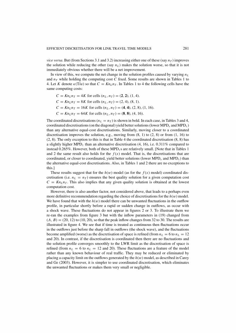
However, there is also another factor, not considered above, that leads to a perhaps evenmore definitive recommendation regarding the choice of discretisations for the h(w) model.We have found that with the h(w) model there can be unwanted fluctuations in the outflowprofile, in particular shortly before a rapid or sudden change in outflows, as occur witha shock wave. These fluctuations do not appear in figures 2 or 3. To illustrate them were-ran the examples from figure 3 but with the inflow parameters in (19) changed from(A, B) = (20, 12) to (10, 20), so that the peak inflow changes from 32 to 30. The results areillustrated in figure 4. We see that if time is treated as continuous then fluctuations occurin the outflows just before the sharp fall in outflows (the shock wave), and the fluctuationsbecome amplified (worse) as the discretisation of space is refined (from nL = 6 to nL = 12and 20). In contrast, if the discretisation is coordinated then there are no fluctuations andthe solution profile converges smoothly to the LWR limit as the discretisation of space isrefined (from nL = 6 to nL = 12 and 20). These fluctuations are a feature of the modelrather than any known behaviour of real traffic. They may be reduced or eliminated byplacing a capacity limit on the outflows generated by the h(w) model, as described in Careyand Ge (2003). However, it is simpler to use coordinated discretisation, which eliminatesthe unwanted fluctuations or makes them very small or negligible.

282 CAREY AND GE

(a)

(b)

Figure 4. Outflow profiles from the τ = h(w) model, with the same settings as figure 3 but with different inflowprofile (19), using (A, B) = (10, 20). (a) Solutions based on continuous time (nT = 640) and (b) Solutions basedon coordinated discretisation.

3.4. Coordinated space and time discretisation

Since the above results and discussion recommend using coordinated discretisation, weconsider how solutions from coordinated discretisation respond to refining the discretisation


(a) (b)

(c) (d)

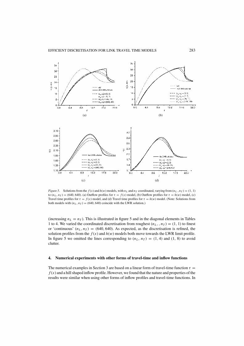
Figure 5. Solutions from the f (x) and h(w) models, with nL and nT coordinated, varying from (nL , nT ) = (1, 1)to (nL , nT ) = (640, 640). (a) Outflow profiles for τ = f (x) model, (b) Outflow profiles for τ = h(w) model, (c)Travel time profiles for τ = f (x) model, and (d) Travel time profiles for τ = h(w) model. (Note: Solutions fromboth models with (nL , nT ) = (640, 640) coincide with the LWR solution.)

(increasing nL = nT ). This is illustrated in figure 5 and in the diagonal elements in Tables1 to 4. We varied the coordinated discretisation from roughest (nL , , nT ) = (1, 1) to finestor ‘continuous’ (nL , nT ) = (640, 640). As expected, as the discretisation is refined, thesolution profiles from the f (x) and h(w) models both move towards the LWR limit profile.In figure 5 we omitted the lines corresponding to (nL , nT ) = (1, 4) and (1, 8) to avoidclutter.

4. Numerical experiments with other forms of travel-time and inflow functions

The numerical examples in Section 3 are based on a linear form of travel-time function τ =f (x) and a hill shaped inflow profile. However, we found that the nature and properties of theresults were similar when using other forms of inflow profiles and travel-time functions. In

284 CAREY AND GE

particular, the direction in which MPDv and MPDτ and the graphs of the solutions change,in response to refining the discretisation of time or space, is the same as in Section 3. Also,the fluctuations discussed in the last paragraph of Section 3.3 and the recommendations thatcoordinated discretisation be used, are as in Section 3.

Rather than illustrate all of this again using various travel-time and inflow functions wewill set out three examples and illustrate only some aspects of these. In these examples weintroduce ‘plateau’ shaped inflow profiles, and a nonlinear (quadratic) travel-time functionτ = f (x), together with the corresponding form of τ = h(w). The inflow profiles wereagain chosen to avoid sharp changes in the inflow rate.

We present results obtained using coordinated discretisation and, for comparison, resultsobtained using the same numbers of link segments but treating time as continuous (thatis, an arbitrarily large number of time steps). We refer to these as the ‘coordinated’ and‘continuous’ cases (‘coord’ and ‘cont’ for short) respectively in Tables 5 to 7 and figures 6to 8 below. (Recall that the coordinated case corresponds to the diagonal in Tables 1 to 4

(a) (b)

(c) (d)

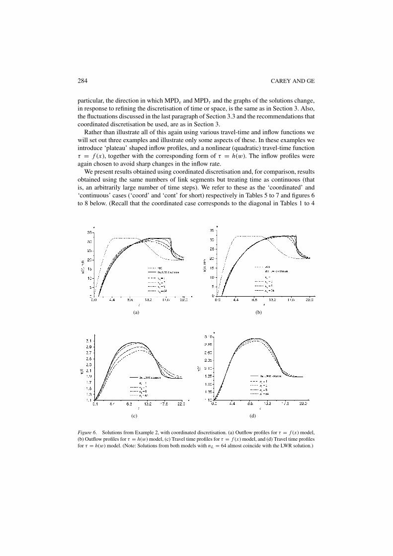
Figure 6. Solutions from Example 2, with coordinated discretisation. (a) Outflow profiles for τ = f (x) model,(b) Outflow profiles for τ = h(w) model, (c) Travel time profiles for τ = f (x) model, and (d) Travel time profilesfor τ = h(w) model. (Note: Solutions from both models with nL = 64 almost coincide with the LWR solution.)


Table 5. Mean percentage deviation of the solution profiles from the LWR solution in figure 6.

Number of segments, nL 1 2 8 64Length of segments, �z 1.2 0.6 0.15 1.875 × 10−2

Time step size (�t) Coord Cont Coord Cont Coord Cont Coord Cont

τ = f (x) MPDv 9.420 9.244 6.714 6.411 2.615 2.421 0.390 0.341

MPDτ 9.224 10.835 5.456 6.293 1.490 1.711 0.153 0.173

τ = h(w) MPDv 4.499 2.518 2.895 1.486 0.942 0.445 0.103 0.193

MPDτ 2.909 1.566 1.448 0.594 0.315 0.077 0.031 0.024


Number of segments, nL 1 2 8 64Length of segments �z 1.2 0.6 0.15 1.875 × 10−2


τ = f (x) MPDv 7.814 7.492 5.262 4.917 1.851 1.677 0.222 0.196

MPDτ 7.331 8.449 4.104 4.676 1.083 1.211 0.116 0.119

τ = h(w) MPDv 4.224 1.943 2.588 1.261 0.821 0.550 0.089 0.414

MPDτ 2.739 1.208 1.405 0.472 0.317 0.070 0.029 0.025


Number of segments, nL 1 2 8 64Length of segments, �z 1.2 0.6 0.15 1.875 × 10−2


Computing cost KnL nT 1K 1MK 4K 2MK 64K 8MK 642 K 64MK

τ = f (x) MPDv 6.203 5.779 4.099 3.777 1.431 1.291 0.162 0.175

MPDτ 5.984 6.713 3.329 3.716 0.934 1.007 0.111 0.113

τ = h(w) MPDv 3.511 1.757 2.054 1.048 0.621 0.506 0.0621 0.410

MPDτ 2.471 0.952 1.278 0.402 0.305 0.056 0.030 0.025

and the continuous case corresponds to the final column in Tables 1 to 4.) In both cases,we divided the link into 1, 2, 4, 8, 16 and 640 segments in successive runs. For coordinateddiscretisation this meant dividing the time horizon [0, 24] into 20, 40, 80, 160, 320 and12,800 time intervals respectively. As before, to generate the benchmark profiles of outflowand travel time from the LWR model we divided the time horizon into a very large numberof time intervals (12,800).

Example 2. With plateau shaped inflow profile and linear form of τ = f (x).

286 CAREY AND GE

In Section 3 we assumed a hill shaped inflow profile. In this example we instead assumea plateau shaped inflow profile as follows

u(t) =

(A + B) sin(π t/10) 0 ≤ t < 5A + B 5 ≤ t < 10A + B sin5(π (t + 2)/24) 10 ≤ t ≤ 22

(20)

in veh/min, where A = 20 and B = 12 are assumed. (This is obtained from the hill shapedprofile (19) by holding the peak value fixed from t = 5 to 10.) We use the same travel-time models as in Section 3, that is (1) and (2), with a = 1.1 min, b = 0.02 min/veh andL = 1.2 km. The generated solution profiles are presented in figure 6, and the correspondingvalues of MPDs are listed in Table 5.

Example 3. With plateau shaped inflow profile and quadratic form of τ = f (x).

The previous experiments have all used a linear travel-time function τ = f (x) hence wehere instead use the nonlinear travel-time models (4) and (6), with a = 1.1 min, b = 0.02veh/min, c = 10−2 veh/min2 and L = 1.2 km. We use the same shaped inflow profile as inExample 2 but with the peak flow reduced from 32 to 22 (A = 10, B = 12). The resultingsolution profiles are shown in figure 7 and the MPDs in Table 6.

Example 4. With hill shaped inflow profile and quadratic form of τ = f (x).

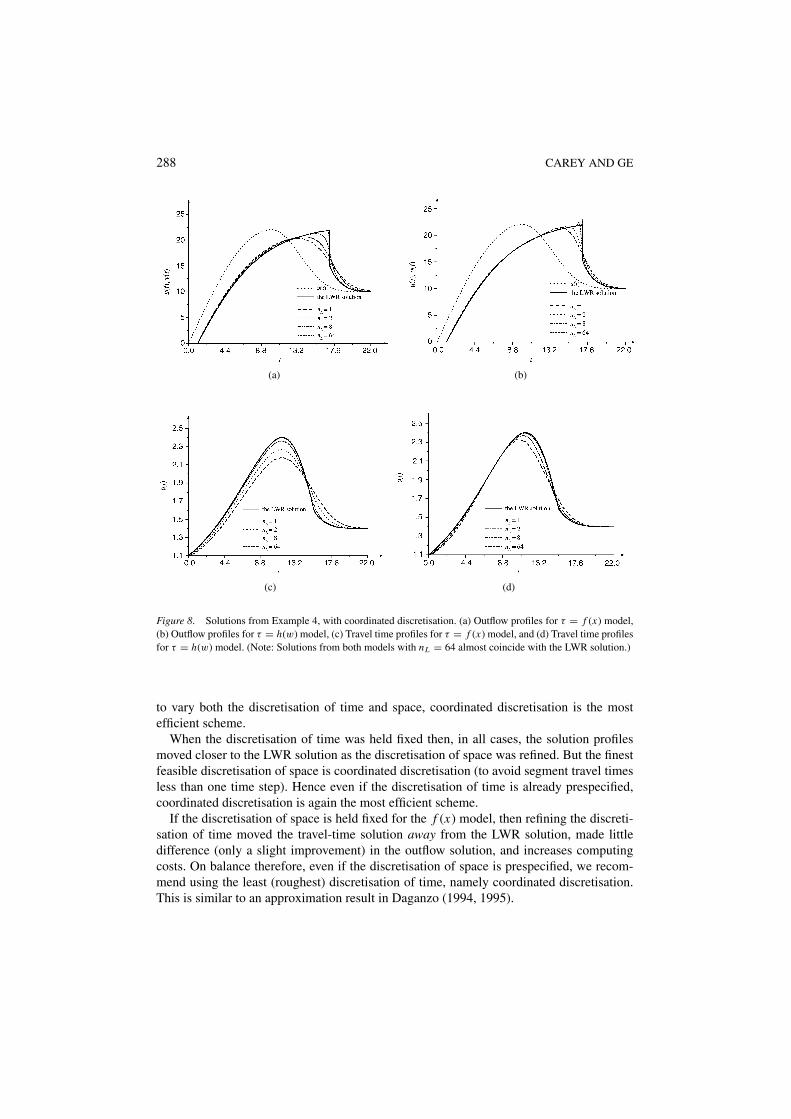
Section 3 assumed a hill shaped inflow profile with a linear travel-time model τ = f (x).Here we show that similar convergence results are obtained assuming a nonlinear travel-time model τ = f (x) with a similar inflow profile. We assume the nonlinear travel-timemodels (4) and (6), as in Example 3, and the inflow profile (19) with A = 10 and B = 12.We repeated the same experiments as in Examples 2 and 3 and the resulting solution profilesare shown in figure 8 and the MPDs in Table 7.

The characteristics of the results in Tables 5 to 7 are basically the same as already notedfor the example in Section 3.2 based on comparing the diagonal elements and final columnin Tables 1 to 4. In all three Tables (5 to 7), the solutions for the h(w) model are in all casescloser to the LWR benchmark (as measured by MPDs) when time is treated as continuousthan when coordinated discretisation is used. However, it must be emphasised this reductionin the MPDs is obtained at a cost of greatly increased computing time (KnLnT ): see thirdrow of Table 7. For the “continuous” case we used a very large number of time intervals (callit M) instead of the minimum number implied by coordinated discretisation (nT = 1, 2, 8and 64 as shown in first row of Table 7). Instead of using continuous time, or anythingapproximating continuous time, a much greater reduction in MPDs can be obtained, for thesame computing cost, by refining the discretisation of time and space together, in coordinateddiscretisation.

The above observation applies even more strongly in the case of the f (x) model. In thatmodel, in all cases, coordinated discretisation yields smaller MPDs for link travel timesand has a lower computing cost than using continuous time (see third row from bottom inTables 5 to 7).


(a) (b)

(c) (d)


5. Concluding remarks

We considered the effects of varying the discretisation of time and space (the link length)used in solving the link travel-time models τ (t) = f (x(t)) and τ (t) = h(w(t)) set out inSection 2. To compare the discretisation schemes numerically we introduced various linktravel-time functions and link inflow functions. We also introduced measures of quality of thesolutions (closeness to the LWR solutions) and a measure of computing cost. We considereda homogeneous link without obstructions or restrictions to flow or traffic controls. For thatcase we note that both models yield the same solution as the LWR model if the discretisationof both space and time are refined to the continuous limit. Some of the remarks below areexplained further in Section 3.3.

For the f (x) model we found (Sections 3.3 and 4) that, for any given level of computingcost, the best approximation to the LWR solution was always obtained by using coordinateddiscretisation. The same was almost always true for the h(w) model. Thus, if we are free

288 CAREY AND GE

(a) (b)

(c) (d)


to vary both the discretisation of time and space, coordinated discretisation is the mostefficient scheme.

When the discretisation of time was held fixed then, in all cases, the solution profilesmoved closer to the LWR solution as the discretisation of space was refined. But the finestfeasible discretisation of space is coordinated discretisation (to avoid segment travel timesless than one time step). Hence even if the discretisation of time is already prespecified,coordinated discretisation is again the most efficient scheme.

If the discretisation of space is held fixed for the f (x) model, then refining the discreti-sation of time moved the travel-time solution away from the LWR solution, made littledifference (only a slight improvement) in the outflow solution, and increases computingcosts. On balance therefore, even if the discretisation of space is prespecified, we recom-mend using the least (roughest) discretisation of time, namely coordinated discretisation.This is similar to an approximation result in Daganzo (1994, 1995).


If the discretisation of space is held fixed for the h(w) model, then refining the dis-cretisation of time moved the solution profiles closer to the LWR solution. Hence, if thediscretisation of space is prespecified, the fineness of discretisation to use depends on achoice or trade-off between quality of the solution and the computing cost. It is notable thatit is only in this case (the h(w) model with the discretisation of space prespecified) thatthere is such a trade-off. In all other cases, coordinated discretisation either gave a lowercost for a given quality of solution, or a better quality of solution for a given cost. However,even in the present case, we recommend coordinated discretisation for another reason. Thatis, it avoids (or reduces) a fluctuation or ‘spike’ that can otherwise occur in solutions of thediscretised h(w) model shortly before a sharp change in outflows, such as a shock wave.

An important special case of the two preceding paragraphs occurs for so called whole-linkDTA models. As noted in the introduction, whole-link models for DTA are usually formu-lated as continuous time models and solved using a fine discretisation of time. However, thecoordinated discretisation recommended for the f (x) and h(w) models in the preceding twoparagraphs implies using the roughest discretisation of time, setting the time steps equal tothe free flow travel time for the whole link.

Finally, we note that for any given discretisation of time and space, the solution of theh(w) was in all cases closer to the LRW solution, as measured by the MPDs, than thesolution of the f (x) model: the percentage difference from the LWR solution was usuallya few times smaller.

Acknowledgment

This research was supported by UK Engineering and Physical Sciences Research Coun-cil (EPSRC) research grants GR/L80904 and GR/R/70101, which the authors gratefullyacknowledge.

References

Adamo, V., V. Astarita, M. Florian, M. Mahut, and J.H. Wu. (1999). “Modelling the Spill-Back of Congestion inLink Based Dynamic Network Loading Models: A Simulation Model with Application.” In Proceedings of the14th International Symposium on Transportation and Traffic Theory, A. Ceder (ed.), Elsevier, pp. 555–573.

Astarita, V. (1995). “Flow Propagation Description in Dynamic Network Loading Models.” In Proceedings of IVInternational Conference on Application of Advanced Technologies in Transportation Engineering (AATT), Y.J.Stephanedes and F. Filippi (eds.), ASCE, pp. 599–603.

Astarita, V. (1996). “A Continuous Time Link Model for Dynamic Network Loading Based on Travel TimeFunction.” In Proceedings of the 13th International Symposium on Theory of Traffic Flow, J.-B. Lesort (ed.),Elsevier, pp. 79–102.

Carey, M. and Y.E. Ge. (2001). “Convergence of Whole-Link Travel Time Models.” Faculty of Business andManagement, University of Ulster, Northern Ireland, BT7 0QB.

Carey, M. and Y.E. Ge. (2003). “Comparing Whole-Link Travel-Time Models.” Transportation Research 37B,905–926.

Carey, M., Y.E. Ge, and M. McCartney. (2003) “A Whole-Link Travel-Time Model with Desirable Properties.”Transportation Science 37, 83–96.

Carey, M. and M. McCartney. (2002). “Behaviour of a Whole-Link Travel Time Model Used in Dynamic TrafficAssignment.” Transportation Research 36(1), 83–95, 2002.

290 CAREY AND GE

Daganzo, C.F. (1994). “The Cell Transmission Model: A Dynamic Representation of Highway Traffic Consistentwith the Hydrodynamic Theory.” Transportation Research 28B, 269–287.

Daganzo, C.F. (1995). “A Finite Difference Approximation of the Kinematic Wave Model of Traffic Flow.”Transportation Research 29B, 261–276.

Friesz, T.L., D. Bernstein, T.E. Smith, R.L. Tobin, and B.W. Wie. (1993). “A Variational Inequality Formulationof the Dynamic Network User Equilibrium Problem.” Operations Research 41, 179–191.

Lighthill, M.J. and G.B. Whitham. (1955). “On Kinematic Waves. I: Flow Movement in Long Rivers II: A Theoryof Traffic Flow on Long Crowded Roads.” In Proceedings of the Royal Society A 229, 281–345.

Newell, G.F. (1988). “Traffic Flow for the Morning Commute.” Transportation Science 22, 47—58.Ran, B., N.M. Rouphail, A. Tarko, and D.E. Boyce. (1997). “Toward a Class of Link Travel Time Functions for

Dynamic Assignment Models on Signalized Networks.” Transportation Research 31B, 277–290.Richards, P.I. (1956). “Shock Waves on the Highway.” Operations Research 4, 42–51.Wu J.H., Y. Chen, and M. Florian. (1995). “The Continuous Dynamic Network Loading Problem: A Mathematical

Formulation and Solution Method.” Presented at the 3rd EURO WORKING GROUP Meeting on Urban trafficand transportation, Barcelona, Sept., pp. 27–29.

Wu, J.H., Y. Chen, and M. Florian. (1998). “The Continuous Dynamic Network Loading Problem: A MathematicalFormulation and Solution Method.” Transportation Research 32B, 173–187.

Xu, Y.W., J.H. Wu, M. Florian, P. Marcotte, and D.L. Zhu. (1999). “Advances in the Continuous Dynamic NetworkLoading Problem.” Transportation Science 33, 341–353.

Zhu, D. and P. Marcotte. (2000). “On the Existence of Solutions to the Dynamic User Equilibrium Problem.”Transportation Science 34, 402–414.

Reproduced with permission of the copyright owner. Further reproduction prohibited without permission.

Documents

Efï¬cient Discretisation for Link Travel Time Models