Embed Size (px)
Citation preview

Course Notes
High Performance Computing Systems and Enabling Platforms
Marco Vanneschi © - Department of Computer Science, University of Pisa
Part 2
Parallel Architectures
This Part deals with a systematic treatment of parallel MIMD (Multiple Instruction Stream Multiple Data
Stream) architectures, in particular shared memory multiprocessors and distributed memory multicomputers.
In Section 1 the main characteristics of both kinds of architectures are introduced and discussed, along with
some relevant issues at the state-of-the-art and in perspective, notably multi-/many-core chips. Section 2 is
dedicated to limited-degree interconnection networks suitable for highly parallel machines: topologies,
technologies, routing and flow control strategies, bandwidth and latency evaluation. Interconnection network
characteristics are used in Section 3 to develop cost models for multiprocessors (shared memory access
latency) and multicomputers (inter-node communication latency). Sections 4 and 5 study and evaluate the
run-time support of parallel computation mechanisms for both classes of MIMD architectures, respectively.
The main issues are related to the exploitation of memory hierarchies and cache coherence, synchronization
and locking, interprocess communication mechanisms for shared memory and distributed memory machines
and their architectural supports, and cost models of interprocess communication.
Contents
1. MIMD parallel architectures ......................................................................................................... 3
1.1 Processing nodes ...................................................................................................................................... 4
1.2 Interconnection networks ......................................................................................................................... 6
1.3 Shared memory multiprocessors .............................................................................................................. 9 1.3.1 Shared memory ..................................................................................................................................................... 9 1.3.2 Multiprocessor taxonomy ................................................................................................................................... 10 1.3.3 Mapping parallel programs onto SMP and NUMA architectures ....................................................................... 13 1.3.4 High-bandwidth shared memory and multiprocessor caching ............................................................................ 16 1.3.5 Cache coherence ................................................................................................................................................. 18 1.3.6 Interleaved memory bandwidth and scalability upper bound .............................................................................. 22 1.3.7 Software lockout ................................................................................................................................................. 25
1.4 Multicomputers ...................................................................................................................................... 26
1.5 Multicore/manycore examples ............................................................................................................... 28 1.5.1 General-purpose architectures: current, low parallelism chips ............................................................................ 28 1.5.2 Experimental, highly parallel architectures on chip ............................................................................................ 31 1.5.3 Network Processors on chip ................................................................................................................................ 32 1.5.4 General-purpose multicore architectures with application-oriented coprocessors .............................................. 33
2. Interconnection networks............................................................................................................. 35
2.1 Network topologies ................................................................................................................................ 35
2.2 Properties of interconnection networks .................................................................................................. 38
2.3 Buses and crossbars ............................................................................................................................... 40
2
2.4 Rings, multi-rings, meshes and tori........................................................................................................ 42
2.5 Routing and flow control strategies ....................................................................................................... 42 2.5.1 Routing: path setup and path selection ................................................................................................................ 43 2.5.2 Flow control and wormhole routing .................................................................................................................... 45 2.5.3 Switching nodes for wormhole networks ............................................................................................................ 45 2.5.4 Communication latency of structures with pipelined flow control...................................................................... 46
2.6 k-ary n-cube networks ............................................................................................................................ 47 2.6.1 Characteristics and routing.................................................................................................................................. 47 2.6.2 Cost model: base latency under physical constraints .......................................................................................... 48
2.7 k-ary n-fly networks ............................................................................................................................... 51 2.7.1 Basic characteristics ............................................................................................................................................ 51 2.7.2 Formalization of k-ary n-fly networks ................................................................................................................ 52 2.7.3 Deterministic routing algorithm for k-ary n-fly networks ................................................................................... 53
2.8 Fat Trees ................................................................................................................................................ 54 2.8.1 Channel capacity: from trees to fat trees ............................................................................................................. 54 2.8.2 Average distance ................................................................................................................................................. 54 2.8.3 Generalized Fat Tree ........................................................................................................................................... 55
3. Cost models for MIMD architectures ......................................................................................... 57
3.1 Shared memory access latency in multiprocessors ................................................................................ 57 3.1.1 Firmware messages in multiprocessor interconnection networks ....................................................................... 57 3.1.2 Memory access base latency ............................................................................................................................... 60 3.1.3 Under-load memory access latency .................................................................................................................... 62 3.1.4 On parallel programs mapping and structured parallel paradigms ...................................................................... 73
3.2 Inter-node communication latency in multicomputers ........................................................................... 75 3.2.1 Performance measures for low dimension k-ary n-cubes .................................................................................... 75 3.2.2 Performance measures for Generalized Fat Trees ............................................................................................... 77
4. Shared memory run-time support of parallel programs ........................................................... 80
4.1 Summary of uniprocessor run-time support of interprocess communication ......................................... 80
4.2 Locking .................................................................................................................................................. 84 4.2.1 Indivisible sequences o memory accesses ........................................................................................................... 85 4.2.2 Lock – unlock implementations .......................................................................................................................... 88 4.2.3 Locked version of interprocess communication run-time support ...................................................................... 90
4.3 Low-level scheduling ............................................................................................................................. 92 4.3.1 Preemptive wake-up in anonymous processors architectures ............................................................................. 92 4.3.2 Process wake-up in dedicated processors architectures ...................................................................................... 93
4.4 Run-time support and cache coherence .................................................................................................. 93 4.4.1 Automatic cache coherence through Invalidation ............................................................................................... 94 4.4.2 Algorithm-dependent cache coherence ............................................................................................................... 97
4.5 Cost model of interprocess communication ........................................................................................... 98
4.6 Communication processor.................................................................................................................... 100
5. Distributed memory run-time support to parallel programs ................................................. 102
6. Questions and exercises .............................................................................................................. 106

3
1. MIMD parallel architectures
MIMD (Multiple Instruction Stream Multiple Data Stream) architectures are the most
widely adopted high-performance machines. They are inherently general-purpose, and
range from medium-low parallelism servers and PC/workstation clusters, to massively
parallel (MPP) enabling platforms. Application parallelism is exploited at the process (or
thread) level, which acts as the intermediate virtual machine for user-oriented parallel
applications, or is the primitive level in which the parallel programming methodology can
be applied directly.
Though medium-high end servers and clusters have been used since several years, MIMD
architectures are now becoming more and more popular owing to the multicore/manycore
evolution/revolution: by now on-chip MIMD architectures are a reality, and the “Moore
law” is expected to be applied to the number of processors (cores), accompanied by a
corresponding evolution of on-chip interconnection networks.
The overall, simplified view of a MIMD architecture is the following:
where the Processing Nodes can be complete computers (CPU, Main Memory, I/O
subsystem), or CPUs possibly with a local memory and/or some limited I/O, or merely
Memory modules.
The interconnection structure, or interconnection network, is able to connect, directly or
indirectly, any pair of processing nodes to exchange firmware messages. Firmware
messages are used by the firmware interpreter and by the process run-time support, and
must not be confused with messages exchanged among application processes at the process
level. That is, firmware messages are an architectural feature to implement shared memory
accesses, or communications between computer nodes or between CPU nodes, according
to the architecture class.
For the moment being, we refer to homogeneous architectures, i.e. composed of N identical
computer nodes or CPU nodes. However, heterogeneous architectures are emerging as a
powerful alternative, especially for very large platforms configurations.
Basically, we distinguish between two main MIMD classes:
1. Shared memory architectures, or multiprocessors,
2. Distributed memory architectures, or multicomputers.
. . . . . . Processing Node
0
Processing Node
i
Processing Node
N-1
Interconnection Network
4
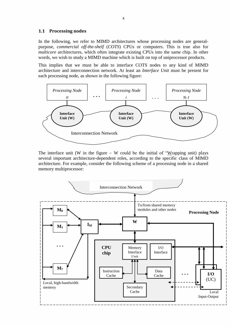
1.1 Processing nodes
In the following, we refer to MIMD architectures whose processing nodes are general-
purpose, commercial off-the-shelf (COTS) CPUs or computers. This is true also for
multicore architectures, which often integrate existing CPUs into the same chip. In other
words, we wish to study a MIMD machine which is built on top of uniprocessor products.
This implies that we must be able to interface COTS nodes to any kind of MIMD
architecture and interconnection network. At least an Interface Unit must be present for
each processing node, as shown in the following figure:
The interface unit (W in the figure W could be the initial of “Wrapping unit) plays
several important architecture-dependent roles, according to the specific class of MIMD
architecture. For example, consider the following scheme of a processing node in a shared
memory multiprocessor:
Local
Input-Output
Local, high-bandwidth
memory
. . . . . . Processing Node
0
Processing Node
i
Processing Node
N-1
Interconnection Network
Interface
Unit (W)
Interface
Unit (W)
Interface
Unit (W)
To/from shared memory
modules and other nodes
Data
Cache
Instruction
Cache
Memory
Interface
Unit
CPU
chip
W
M0
M1
M7
IM
. . .
. . .
Interconnection Network
Processing Node
Secondary
Cache
I/O
(UC)
I/O
Interface

5
Node Interface Unit
An off-the-shelf CPU chip is connected to the “rest of the world” through its primitive
external interfaces, in the figure the Memory Interface and the I/O interface (e.g., I/O Bus).
The interface unit W is directly connected to the Memory Interface, so it is able to
intercept all the external memory requests and to transform them into proper firmware
messages to/from the various sections of the architecture:
i) external firmware messages: through the interconnection network all the shared
memory supports are visible as destinations or as sources, all well as some specific
I/O units belonging to the other nodes (Memory Mapped I/O);
ii) internal firmware messages, exchanged with the local memory (where present) and
the local I/O.
For example, in case i), consider a read-request directed to the main memory (it may be the
request of a single word or, more in general, of a cache block). According to the physical
address, W is able to distinguish whether the request has to be forwarded: a) to the local
memory or to the local I/O, or b) to the external shared memory. In case a) very few
modifications are done to the firmware message received from the CPU (physical address,
memory operation type, and other synchronization or annotation bits). In case b), the
request is transformed into a firmware message (consisting in one or few words)
containing all the architecture-dependent information: the information received by the CPU
are enriched by the message header, i.e. network routing and flow control information
(source node identifier, destination node identifier, message length, message type, and
possibly others), some of which are derived from the CPU request itself (e.g. the
destination memory module identifier is a part of the physical address). In both cases a)
and b), W is able to serve other requests simultaneously, possibly from other nodes,
including the reply from the main memory (single word or cache block) which is returned
to the CPU. In some architectures, the Interface Unit could also be a complex subsystem,
consisting of several units.
Communication Unit
In the figure, an I/O unit, called Communication Unit (UC), is provided for direct
interprocessor communications support.
Though, in a multiprocessor, the majority of run-time support information are present in
shared memory, there are some cases in which asynchronous I/O messages are preferred.
Two main types of interprocessor communications are used:
for processor synchronization, i.e. for the implementation of some locking
mechanism,
for process low-level scheduling, notably for decentralized process wake-up or
processor preemption.
6
Let us assume that CPUs are memory mapped I/O machines (e.g., D-RISC). An
interprocessor communication from node Ni to node Nj begins with the transfer of the
message from CPUi to UCi through one or more Store instructions. UCi communicates the
message to UCj through the node interface unit and the interconnection network. UCj
transforms the received message into an interrupt to CPUj, where the interrupt handler will
be executed as usually.
CPU facilities for MIMD architectures
The COTS uniprocessor reutilization is not always free or easy. Some additional MIMD
facilities, notably for the correct and/or efficient implementation of the firmware
parallelism and of the process run-time support, must be present in the corresponding
uniprocessor architecture at the assembler and/or firmware level. In other words, a certain
knowledge of the potential utilization in a MIMD architecture must have been foreseen in
the corresponding uniprocessor architecture. Notable examples of facilities for shared
memory architectures are:
especially for highly parallel machines, the physical address space must be
extendable to very large capacities, for example 1 Tera (40-bit physical address) till
256 Tera (48-bit physical address). Though this issue has no impact at the
assembler machine level, it requires proper firmware support, notably in MMU and
in the chip interface, and the proper definition of the address translation function;
locking mechanisms, or other synchronization mechanisms, require special
assembler instructions or annotations in assembler instructions, as well as proper
information at the CPU interface (indivisibility bit);
cache management multiprocessor-dependent options require special instructions or
annotations, as well as proper information at the CPU interface (e.g. firmware
structures and directives for cache coherence).
1.2 Interconnection networks
In general, highly parallel architectures utilize limited degree networks, in which a
processing node is directly connected to only a small subset of nodes, or it is indirectly
connected to any other node through an intermediate path of switching nodes with few
neighbors. Correspondingly, interconnection networks can be classified in:
direct, or static, networks,
indirect, or dynamic, networks.
In a direct network, point to point dedicated links connect the processing nodes in some
fixed topology. Of course, messages can be routed to any processing node which is not
directly connected. Each network node, also called switch node, is connected to one and
only one processing node, possibly through the node interface unit (logically, W is not
necessary if the network node plays this role too). Notable examples of limited-degree
direct networks for parallel architectures are:
Rings,
Meshes and Tori (toroidal meshes),
Cubes (k-ary n-cubes),
shown in figure 1.

7
Figure 1 : examples of direct network topologies
In an indirect network, processing nodes are not directly connected; they communicate
through intermediate switch nodes, or simply switches, each of which has a limited number
of neighbors. In general, more than one switch is used to establish a communication path
between any pair of processing nodes. These structures are also denoted as dynamic
networks, since they allow the interconnection pattern among the network nodes to be
varied dynamically through the proper cooperation of switching units. Buses and crossbars
are indirect networks at the possible extremes. Notable examples of limited-degree indirect
networks for parallel architectures are:
Multistage networks,
Butterflies (k-ary n-fly),
Trees and Fat Trees,
shown in the figure 2.

8
Figure 2: examples of indirect network topologies
N
0
N
1
N
2
N
3
N
4
N
5
N
6
N
7

9
The various topologies are characterized by the following orders of magnitude of
communication latencies for firmware messages (N = number of processing nodes):
Crossbar (not limited-degree network): O(1)
Buses, Rings: O(N)
Meshes, 2-dimension cubes: O( 𝑁)
Hypercubes, multistage, butterflies, trees and fat trees: O(log N).
More precisely, these are the latencies evaluated in absence of contention (base latency). In
Section 2 we will describe the various kinds of networks in detail, and evaluate the cost
model for the base latency and for the under-load latency.
1.3 Shared memory multiprocessors
In a multiprocessor architecture, N processors (better: CPUs) share the main memory (in
general realized according to a high bandwidth organization). The following is a
simplified, abstract view of a shared memory multiprocessor:
As an alternative, in multicore chips some lower levels of the memory hierarchy (secondary
cache, tertiary cache) can be shared among the all the CPUs (cores) or groups of CPUs.
1.3.1 Shared memory
The shared memory characteristic of multiprocessors means that any processor is able to
address any location of main memory. That is, the result of the translation of a logical
address, generated by any processor, can be any physical address of the main memory.
Thus, processors are allowed
a) to physically share information (shared data structures or objects). More precisely:
distinct processes can refer data which are shared in a primitive way, i.e. physically
shared data in the same physical memory;
. . . . . .
CPU0
CPUi
CPUN-1
Shared main memory or memory hierarchy
Interconnection network:
processor-memory and processor-processor
W W W
Node 0
Node i
Node N-1

10
b) to have access to a common memory acting as a sort of repository for any
information, including private information too, i.e. information (programs and data)
that are private of processes and are not shared with other processes.
Notice that these characteristics are peculiar of the uniprocessor architecture too. In fact,
from several respects, multiprocessors can be considered as a parallel extension of
uniprocessors.
The shared memory characteristics is, at the same time, the advantage and the disadvantage
of multiprocessors:
on one hand, it is exploited (as in uniprocessors) to implement an easy-to-design
and potentially efficient run-time support of interprocess cooperation. In fact, the
run-time support is an extension of the basic solutions studied for uniprocessors in
Part 1, Sect. 3, the extensions being due to correctness (consistency) and to
efficiency reasons;
on the other hand, shared memory is the primary source of performance
degradation, since the access to shared memory modules and/or shared data cause
congestion. That is, formally the system can be modeled as a client-server queueing
system, where the clients are processors and the servers are shared memory
modules. The utilization factor of each memory module could be so high (though
less than one) that, in absence of proper optimization techniques, the efficiency and
scalability are relatively low despite a large number of processors is connected.
Moreover, the memory access “base “latency (i.e. without considering congestion)
is (much) higher than in a uniprocessor, because the interconnection network
latency is a function of the number N of processing nodes.
1.3.2 Multiprocessor taxonomy
An useful multiprocessor taxonomy is shown in the following Figure.
Processes to processors mapping refers to the strategy for allocating processes to
processing nodes:
a) dedicated processors: process allocation is decided statically, once for all. That is,
processes are partitioned into N disjoint sets, and each set is allocated to a distinct
processing node at loading time. Thus, a process can be executed only by the same
processor. Explicit reallocation of processes to other nodes is possible at run-time
too, notably for load balancing or fault tolerance, however it is considered a relative
Shared memory multiprocessors
Processes to processors mapping Shared memory organization
Anonymous
processors
Uniform Memory
Access (UMA)
Dedicated processors
Anonymous processors
Non Uniform Memory Access
(NUMA)
11
rare event. In this architecture, each node has its own process Ready List, which is
managed - as in a uniprocessor system - only by the local process set;
b) anonymous processors: no static process allocation exists, thus any process can be
executed by (i.e., it can run on) any processor. Process allocation is dynamically
performed at run-time, i.e., it coincides with the low-level scheduling of processes.
A unique system-wide Ready List exists, from which each processor, in the
context-switch phase, “gets” the process to be executed.
Informally, the anonymous processors architecture is the natural generalization of
uniprocessor. Conceptually, it follows the farm paradigm, with the goal of achieving a
good load balance of processors: processors acts as workers, the low level scheduling is the
abstract emitter functionality, and the Ready List acts as the task stream.
The dedicated processor architecture is a first step towards more distributed architectures
with respect to uniprocessor machines. Conceptually, it follows the functional partitioning
with independent workers paradigm: processors acts as workers, the task stream is thought
of as decomposed into N distinct partitions, and the distribution functionality is statically
established. As known, in principle this paradigm is prone to processors load unbalance,
although this problem is partially alleviated by the number of processes allocated to the
same node, and possibly by periodic reallocations.
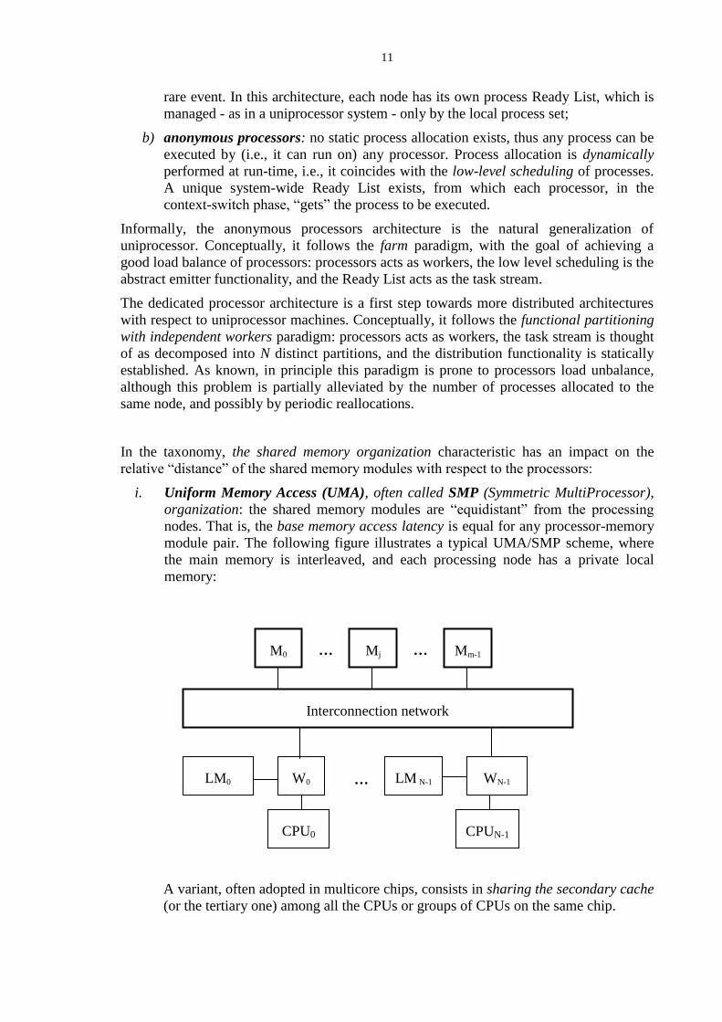
In the taxonomy, the shared memory organization characteristic has an impact on the
relative “distance” of the shared memory modules with respect to the processors:
i. Uniform Memory Access (UMA), often called SMP (Symmetric MultiProcessor),
organization: the shared memory modules are “equidistant” from the processing
nodes. That is, the base memory access latency is equal for any processor-memory
module pair. The following figure illustrates a typical UMA/SMP scheme, where
the main memory is interleaved, and each processing node has a private local
memory:
A variant, often adopted in multicore chips, consists in sharing the secondary cache
(or the tertiary one) among all the CPUs or groups of CPUs on the same chip.
… … M0
…
Mj Mm-1
Interconnection network
W0
CPU0
LM0 WN-1
CPUN-1
LM N-1
12
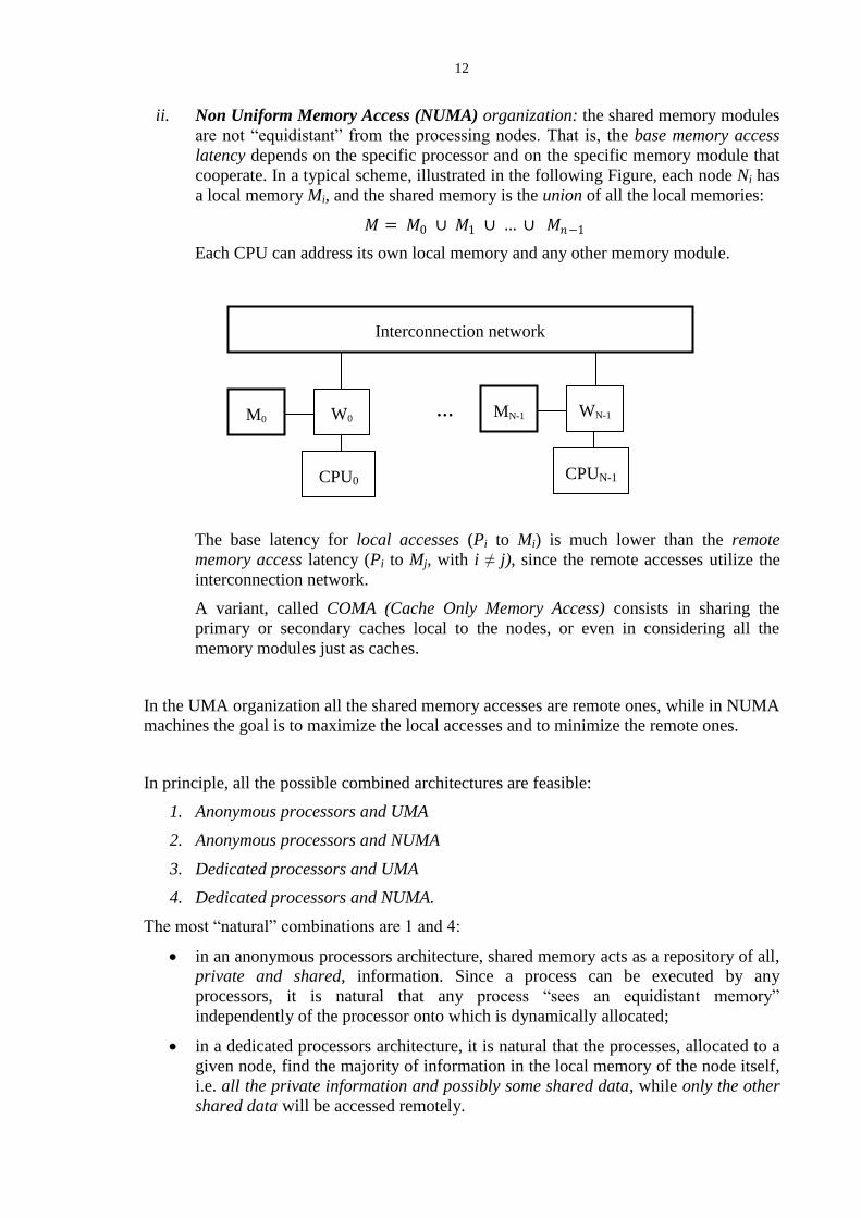
ii. Non Uniform Memory Access (NUMA) organization: the shared memory modules
are not “equidistant” from the processing nodes. That is, the base memory access
latency depends on the specific processor and on the specific memory module that
cooperate. In a typical scheme, illustrated in the following Figure, each node Ni has
a local memory Mi, and the shared memory is the union of all the local memories:
𝑀 = 𝑀0 ∪ 𝑀1 ∪ … ∪ 𝑀𝑛−1
Each CPU can address its own local memory and any other memory module.
The base latency for local accesses (Pi to Mi) is much lower than the remote
memory access latency (Pi to Mj, with i ≠ j), since the remote accesses utilize the
interconnection network.
A variant, called COMA (Cache Only Memory Access) consists in sharing the
primary or secondary caches local to the nodes, or even in considering all the
memory modules just as caches.
In the UMA organization all the shared memory accesses are remote ones, while in NUMA
machines the goal is to maximize the local accesses and to minimize the remote ones.
In principle, all the possible combined architectures are feasible:
1. Anonymous processors and UMA
2. Anonymous processors and NUMA
3. Dedicated processors and UMA
4. Dedicated processors and NUMA.
The most “natural” combinations are 1 and 4:
in an anonymous processors architecture, shared memory acts as a repository of all,
private and shared, information. Since a process can be executed by any
processors, it is natural that any process “sees an equidistant memory”
independently of the processor onto which is dynamically allocated;
in a dedicated processors architecture, it is natural that the processes, allocated to a
given node, find the majority of information in the local memory of the node itself,
i.e. all the private information and possibly some shared data, while only the other
shared data will be accessed remotely.
…
Interconnection network
W0
CPU0
M0 WN-1
CPUN-1
MN-1
13
In the following, unless otherwise stated,
combination 1 will be called SMP multiprocessor,
combination 4 will be called NUMA multiprocessor.
However, though combinations 1 and 4 are the most popular, also combinations 2 and 3
are meaningful and some notable examples exist. The reason lies in the central role that
memory hierarchy and caching play in multiprocessor architectures. Informally, if cache
memories are allocated efficiently (i.e. if processes are characterized by high locality and
reuse) the majority of accesses are performed locally in caches, thus smoothing the
difference between local or remote main memory, which has impact on the block transfer
latency only.
The importance of caching in multiprocessors architectures will be studied deeply in
subsequent Sections.
1.3.3 Mapping parallel programs onto SMP and NUMA architectures
In this Section we reason about some relationships between architectural paradigms (SMP
and NUMA multiprocessors) and structured parallel applications paradigms.
Let us consider a parallelization example, studied according to the methodology of Part 1.
Example specification
We wish to parallelize a sequential process P, which statically encapsulates two
integer arrays, A[M] and B[M] with M = 106, and operates on a stream of integers
x. For each x, P computes
c = x;
i = 0 … M – 1: c = f (c, A[i], B[i])
The obtained c value is sent onto the output stream.
Function f is a black-box of which the calculation time distribution is known: the
uniform distribution in the interval (0 - 20. The average interarrival time is equal
to 105.
Let the following three target architectures, based on the same COTS technology,
be available:
1. NUMA multiprocessor with 128 processing nodes, private secondary cache
of 2 Mega words per node, and local-shared memory of 1G words per node;
2. SMP multiprocessor with 128 processing nodes, private secondary cache of
2 Mega words per node, and equidistant shared main memory of 128G
words;
3. SMP multiprocessor with 128 processing nodes, 16 secondary caches, each
of which is 16 Mega words and is shared by a distinct group of 8 nodes, and
equidistant shared main memory of 128G words.
In any configuration, each processing nodes has a primary data cache of 32K
words, with block size = 8 words, and a communication processor. The
interprocess communication parameters are assumed equal for the three
architectures: Tsetup = 103, Ttrasm = 10
2.
14
Arrays A, B are statically allocated in P, thus they are statically encapsulated (replicated or
partitioned) in the processes of any parallel version.
In any parallel version, the ideal parallelism degree is
𝑛 = 𝑇𝑐𝑎𝑙𝑐
𝑇𝐴=
𝑀 𝑇𝑓
𝑇𝐴= 100
which is lower than the number of available processing nodes.
Two parallel versions can be identified:
a) A farm version with A and B fully replicated in n = 100 workers. Since the emitter and
collector are not bottlenecks (their service time is equal to Tsend(1) = 1,1 x 10³ <<
TA), the effective service time is equal to the ideal one, that is TA. Each worker node
requires a memory capacity equal to the sequential version (about 2 Mega words,
referring to data only), thus the whole memory capacity is equal to about 200 Mega
words.
b) For studying a data parallel implementation, we observe that, since no computational
property is known about function f, the M steps, to be executed for each x, are linearly
ordered. Thus, the only applicable data parallel paradigm is the loop-unfolding
pipeline, in which x values enter the first stage and the intermediate stages
communicate the partial c values. The virtual processor version consists of an array
VP[M], where the generic VP[i] encapsulates A[i] and B[i]. By mapping the virtual
processor version onto the actual one with parallelism degree n = 100, each stage
statically encapsulates a partition of A and a partition of B of size M/n = 104 integers.
The ideal service time of each stage is equal to 105, thus the communication latency
Tsend(1) is fully masked by the calculation time. The effective service time is equal to
the ideal one, that is TA. The whole memory capacity is equal to the sequential version
(about 2 Mega words, referring to data only), while each node requires a memory
capacity of about 20K words.
The advantages of the pipeline solution in terms of required memory capacity are obvious.
On the other hand, the pipeline solution is affected by load unbalance problems, due to the
high variance of the calculation time.
The impact of the required memory capacity of both solutions will be studied for the three
architectures.
For this purpose, let us characterize the sequential computation P from the memory
hierarchy utilization viewpoint. For each input steam element x, the same values of A and
B (1 Mega words each) are needed. Thus, A and B are characterized by full reuse, and of
course locality too. We assume that the primary instruction cache is able to store all the
code blocks (function f), thus in the following we focus on the data cache only. The data
cache working set for the sequential abstract machine is given by all the A and B blocks
(about 2 Mega words). This working set can be actually exploited only if the physical
architecture is able to maintain the working set in primary cache permanently (option “not-
deallocate”, if available at the assembler machine level). The uniprocessor equivalent
physical architecture has nodes with primary data cache of 32K words and secondary
cache of 2 Mega words. Thus, the uniprocessor equivalent physical architecture is not able
to exploit the desired working set in primary data cache. The consequence is that the reuse
property is not exploited, thus
2M/primary cachefaults
15
occur during the manipulation of each input stream element x. The effect on P service time
is not evaluated in detail here (it depends on the organization of the block transfer and
other architectural aspects), however we can say that the performance degradation is
meaningful compared to the ideal situation of reuse exploitation.
1. NUMA multiprocessor with 128 processing nodes, private secondary cache of 2 Mega
words per node, and local-shared memory of 1G words per node
1a) Farm solution
The situation is the same of the uniprocessor machine, replicated in every node. The
primary data cache (32K words) has not sufficient capacity to store all the data
working set (2 Mega words). The secondary private cache is strictly sufficient,
provided that no other processes are allocated in the same node. A realistic situation is
that some performance degradation is due to secondary cache faults too, though pre-
fetching is typically applied at this level of memory hierarchy.
In conclusion, the farm solution will be penalized by the whole memory hierarchy
inadequacy with respect to the working set requirements of the computation. The
consequence is a sensible increase in service time. Alternatively, we can re-evaluate
the sequential calculation time Tcalc, taking into account the cache penalties; this leads
to a greater value of the parallelism degree, which has to be compared to the actual
number of processing nodes.
1b) Pipelined data parallel solution
This is a typical case in which the data parallel computation behaves much better than
the sequential one (“hyper-scalability”). In fact, each node is able to maintain the
respective working set partition in data cache permanently, passing from one stream
element to the next, i.e. is able to exploit full reuse. Once loaded into the primary data
cache for the first stream element, the A and B partitions (20K words) are no more
deallocated. We are able to meet a very significant objective of multiprocessor
architectures: the secondary caches and the shared memory itself are scarcely utilized,
except for communications (which, on the other hand, are fully masked by
calculations).
The load unbalance effect can mitigate the advantages of the data parallel solution. In
this application, we can say that the better utilization of memory hierarchy overcomes
the load unbalance effect. However, this issue would deserve an additional
investigation (not discussed here for the sake of brevity).
2. SMP multiprocessor with 128 processing nodes, private secondary cache of 2 Mega
words per node, and equidistant shared main memory of 128G words
2a) Farm solution
The replicated arrays, A and B, are allocated in the shared main memory in 100
copies. They are loaded, at least in part, into the secondary caches once referred for the
first time by the respective workers. The 256K faults generated by each primary data
cache can not always be served by the secondary cache alone, thus a certain fraction of
block transfers the main memory is needed. On the other hand, despite the anonymous
processors characteristic, processor context-switching is a rare event in a well
designed farm program (statistically, emitter, workers and collectors are rarely
blocked, owing also to the load balanced behavior). Thus, the situation is analogous to
the execution on a NUMA architecture, with some additional, marginal degradation.
16
2b) Pipelined data parallel solution
Analogously to the NUMA architecture, reuse of A and B partitions in primary data
caches is fully exploited, once the A and B partitions have been acquired for the first
time. The load unbalance can increase the probability of context-switching, with a
consequent additional degradation with respect to the NUMA architecture, although
the anonymous processor characteristic can marginally mitigate this problem.
3. SMP multiprocessor with 128 processing nodes, 16 secondary caches, each of which
is 16 Mega words and is shared by a distinct group of 8 nodes, and equidistant shared
main memory of 128G words
For this parallel program, we can say that, statistically, the memory hierarchy has the
same performance of architecture 2, since the farm workers or the pipeline stages,
belonging to the same group of 8 nodes, tend to share the respective secondary cache
uniformly. Thus, similar considerations to architecture 2 apply to both the farm and
the data parallel version.
This example shows some important relationships between parallel programming
paradigms and parallel architectures. Notably the following characteristics of parallel
paradigms have a strong impact on the achievable performance:
memory requirements,
load balancing,
predictability of sequential computations.
On the other hand, several architectural issues have to be taken into account, notably:
interprocess communication costs,
non-determinism in process scheduling,
structures for memory hierarchy management, notably block transfer bandwidth
and latency,
options for primary cache management,
strategies for secondary cache management,
1.3.4 High-bandwidth shared memory and multiprocessor caching
As said, multiprocessor performance is limited by the latency of the interconnection
network and of shared memory modules. We distinguish between:
base latency, i.e. without considering the effects of congestion,
under-load latency, i.e. considering the effects of congestion, evaluated according
to a client-server queueing model.
In order to reduce such latencies, modular memory and caching become the most critical
issues. Both techniques aim to decrease the response time, since both the server service
time (utilization factor) and the server latency are improved by applying these techniques.
17
Modular memory
The interleaved memory organization plays a double role in multiprocessors:
a) as in uniprocessor machines, it supports high-bandwidth transfers of cache blocks;
b) peculiarly of multiprocessor machines, it contributes to reduce the memory
congestion (the memory utilization factor).
Jointly, points a) and b) motivate the following memory organization:
1) a modular memory is composed of several groups of modules, called macro-
modules,
2) each macro-module has an interleaved internal organization, for example:
3) macro-modules may be organized, each other,
in an interleaved way, as in the SMP architecture (in the figure: the first
location of module M4 has physical address equal to 4), or
in a sequential way as in a NUMA architecture (in the figure: the first location
of module M4 has a physical address which is equal to the last address of
module M3 incremented by one).
The global effect is high bandwidth for cache block transfers in any architecture (SMP,
NUMA), and reduced contention on equidistant memory modules in SMP machines.
From a technological point of view, a macro-module with h modules, each with k-bit
words, can be realized as just one module with long word, i.e. with hk-bit words
(similarly to superscalar/VLIW architectures). For example, a 256-bit word macro-module
is equivalent to a macro-module composed of 8 interleaved modules with 32-bit words
each.
Often the number of modules, or the number of words in a long word, of a macro-module
coincides with the cache block size (cache “line”).
Caching
Similarly to the interleaved memory organization, caching plays a very important double
role in multiprocessors:
a) as in uniprocessor machines, it contributes to minimize the instruction service time,
b) peculiarly of multiprocessor machines, it contributes to reduce the memory
congestion (the memory utilization factor), as well as the network congestion.
About point b), notice that even relatively slow caches could be accepted (any way, cache
technologies are characterized by relatively low access times too).
Interleaved macro-
module 1
Interleaved macro-
module 2
Interleaved macro-
module 0
M0 M1 M2 M3 M4 M5 M6 M7
. . .
18
The term all-cache architecture will be used for multiprocessors in which any information
is transferred into the primary cache before being used. Many machines are all-cache,
although some systems offer the cache-disabling option in order to avoid that some
information are cached, for example by marking the entries of the process relocation table
with a “cacheable/non cacheable” bit.
1.3.5 Cache coherence
The potential advantages of the all-cache characteristic have an important consequence: the
so-called cache coherence problem. It consists in the need to maintain shared data
consistent in presence of caching. That is, assume that processors Pi and Pj transfer the
same block S from the main memory M into their respective primary caches Ci and Cj:
if S is read-only, no consistency problem arises;
if Pi modifies (at least one word of) S in Ci, then the S copy in Cj becomes
inconsistent (not coherent). This inconsistency cannot be solved by the existence of
S copy in M, because:
o for Write-Back caching, M is inconsistent with respect to Ci,
o but even in a Write-Through system M is not “immediately” consistent with
Ci (i.e., updating S in Ci and updating S in M are not atomic events,
otherwise the Write-Through technique doesn’t make any sense), thus it is
not possible to rely on this writing technique only.
Solutions to this problems have been investigated intensively. We will distinguish between
automatic techniques and non-automatic or algorithm-dependent techniques.
Automatic cache coherence
In many systems, cache coherence techniques are entirely implemented at the firmware
level. Two main automatic techniques are used:
a) Invalidation: at most one copy of a modifiable block S exists in the whole set of
caches. Let Ci be the cache currently storing S; Ci is called the owner of S. If any
other processor Pj tries to acquire S in Cj, then Pj invalidates the Ci copy and Cj
becomes the owner of S. Invalidation has the effect of de-allocating the block. An
optimized version is the following: more than one cache can contain an updated
copy of S, however, if a processor Pj modifies S, than only the copy in Cj becomes
valid, and all the other copies are invalidated;
b) Update: more than one copy of S can be present simultaneously in as many caches.
Each modification of S in Cj is communicated (multicasted) to all other caches in
an atomic manner. That is, all copies of the same block in different caches are
maintained consistent.
19
In both cases, a proper protocol (e.g. the MESI standard and its variants) must exists to
perform the required sequences of actions atomically, i.e. in an indivisible, time-
independent way. At first sight, the Update technique appears simpler, while Invalidation
is potentially affected by a sort of inefficient “ping-pong” effect (two nodes, that try
simultaneously to write into the same block, invalidate each other repeatedly). However,
things are different in the real utilization of cache coherent systems: Update has a
substantially higher overhead, also due to the fact that only a small fraction of nodes
contain the same block. On the other hand, processor synchronization reduces the “ping-
ping” effect substantially, so Invalidation is adopted by the majority of systems.
Moreover, several optimizations have been proposed in order to reduce the number of
invalidations. An example is the MESIF protocol:
a descriptor is maintained in shared memory for each cache block. The descriptor
contains a mask of N bits, where the i-th bit correspond to processor Pi;
if, for block p,
o bit_mask[j] = 0: processor Pj can not have block p in cache Cj;
o bit_mask[j] = 1: it is possible (but not guaranteed) that processor Pj has
block p in cache Cj;
for each p, automatic coherence is applied to processors having the bit_mask = 1.
Automatic cache coherence protocols is studied in detail in a companion document by
Silvia Lametti.
Two main classes of architectural solutions have been developed for automatic caching:
i) Snoopy-based, in which atomicity is achieved merely by means of a hardware
centralization point, notably a single bus (Snoopy Bus). The bus is “snooped” by all
the nodes, so that each node has always updated information about the relevant
state of a block (e.g. modified or not): snooping and broadcast are primitive
operations for the bus structure. This solution is clearly limited to machines with a
low number of processors, and forces the choice of the slowest kind of
interconnection structure;
ii) Directory-based, in which atomicity is achieved by means of protocols on shared
data without relying on hardware centralization points. Each block is associated a
shared data structure, called the block directory entry, which maintains information
about the set of caches that currently contain a block copy and its state.
Broadcast/multicast communications are used only when strictly necessary,
otherwise point-to-point interprocessor communications are employed. Though at
the expense of a substantial overhead in terms of additional shared memory
accesses, this class of solutions aims to solve the cache coherence problems also in
highly parallel multiprocessors with powerful interconnection networks.
Non-automatic or algorithm-dependent cache coherence
This technique is characterized by explicit cache management strategies, which are specific
of the algorithm to be executed, without relying on any automatic architectural support.
Relying on the existence of explicit processor synchronizations and on proper data
structures, it is possible to emulate cache coherence techniques in an efficient way for each
computation, often reducing the number of memory accesses and cache transfers. No
mechanism/structure exists that limit the architecture parallelism.

20
The intuitive pros and cons consist, respectively, in
possible optimizations for the specific algorithm, with respect to the automatic
solutions overhead,
an increased complexity of programming.
Automatic vs non-automatic approaches to cache coherence: synchronization and reuse
In order to better understand relative strengths and weaknesses of automatic and non-
automatic solutions, let us consider some typical situations in parallel or concurrent
applications. We will distinguish shared-objects vs message-passing applications and, for
each model, automatic vs non-automatic approaches.
a) Shared-objects applications
Consider an application expressed (compiled) according to a global environment, i.e.
shared-objects, cooperation model. Consider two or more processes sharing an object A in
mutual exclusion, e.g. each process contains a critical, or indivisible, section S of
operations implying consistent reading and writing of A. Proper synchronization
operations are provided to ensure mutual exclusion of S (see also Sect. 4.2): in turn, such
operations exploit a shared object X (e.g. semaphore, monitor) manipulated in an
indivisible manner:
Process Q ::
…
while (…) do
…
enter_critical_section (X);
A = F(A, …);
exit_critical_section (X);
…
…
Process R :: similar
Process …
Cache coherence has to be applied both to A and to X.
Furthermore, suppose that S is executed many times, for example is contained in a loop.
For this reason, reuse is an important property of both X and A.
Consider the situation in which
i) the critical section S is executed by process Q, running on processor P, and
ii) no other process attempts to execute S before the second execution of S by Q on P.
S

21
a1) Shared objects applications and automatic approach
Once A and X have been transferred into the cache of P during the first execution of S,
owing to assumption ii) an automatic approach is able to naturally exploit reuse: A and X
are still in P cache during the second execution of S, thus automatically avoiding transfer
overhead of objects A and X between the memory hierarchy levels for each iteration.
Instead, if assumption ii) doesn’t hold (other processes execute S between the first and the
second execution of Q), X and A have been automatically invalidated, thus they are not
present in P cache during the second execution of S and must be acquired again.
In other words, the automatic approach aims to perform the block transfers (through
invalidation) in the strictly needed cases only.
a2) Shared objects applications and non-automatic approach
In a non-automatic approach, the simplest design style is to write a code that ensures cache
coherency, but that does not ensure reuse: at the exit of primitives modifying X and at the
exit of S, objects X and A are re-written in main shared memory.
However, more sophisticated design styles can be conceived, making exploitation of reuse
possible in the automatic approach too. Some special operations can be defined which
verify the consistency of X and A and, if objects are modified by other processes, provide a
sort of invalidation by program.
Again, the same power of the automatic approach is possible in the non-automatic case too,
although at the expense of an increased complexity of programming for objects whose
management is visible to the programmer. On the other hand, specific applications can
have peculiar properties according to which optimizations can be recognized in a non-
automatic solution with respect to the automatic case.
b) Message-passing applications
Consider now an application expressed (compiled) according to a local environment, i.e.
message-passing, cooperation model. In this case, in a shared memory architecture, shared
objects belong to the run-time supports of message-passing primitives only
(communication channel descriptors, locking semaphores, target variables, process
descriptors, and so on).
In this case, the programming complexity disadvantage of the non-automatic approach
doesn’t exist, provided that the following strategy is adopted: algorithm-dependent
solutions are applied in the design of the run-time support to concurrency mechanisms, as
it will be done in Sect. 4.4.
In a system with a clear structure by levels, this solution allows the application designer to
neglect the cache coherence problems (as it must be, since the applications should be
developed in an architecture-independent way), while the only instances of the cache
coherence problems are limited to the run-time support of the message-passing concurrent
language in which the applications are expressed or compiled. Thus, explicit cache
coherence strategies are designed for the very limited set of algorithms used in the run-time
support of message-passing primitives only.
Notice that this is true also for the global environment model, at least as far as the
synchronization primitives are concerned (operation acting on X, in the previous example).
Moreover, for such applications, some development frameworks/tools provide primitive
operations to manipulate any shared object, e.g. also A in the previous example. Again, in
22
such cases, the only instances of the cache coherence problems are limited to the run-time
support of the concurrent language in which the applications are expressed or compiled.
The only case in which the non-automatic approach requires additional efforts to the
application programmer is the following one: global environment applications in which
some shared objects (e.g., A in the previous examples) are not manipulated by means of
primitives of the concurrent part of the language, i.e. they are manipulated by usual
mechanisms of sequential languages without any intervention of the concurrent compiler.
In Section 4.4 automatic and non-automatic techniques will be studied and compared in
depth with respect to the interprocess communication run-time support.
False sharing
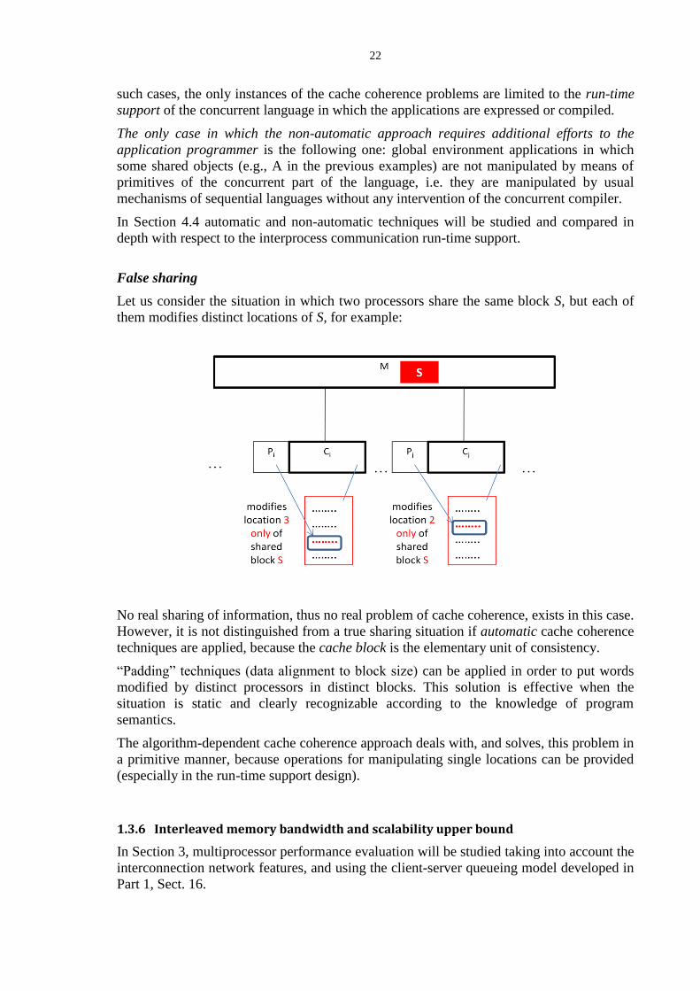
Let us consider the situation in which two processors share the same block S, but each of
them modifies distinct locations of S, for example:
No real sharing of information, thus no real problem of cache coherence, exists in this case.
However, it is not distinguished from a true sharing situation if automatic cache coherence
techniques are applied, because the cache block is the elementary unit of consistency.
“Padding” techniques (data alignment to block size) can be applied in order to put words
modified by distinct processors in distinct blocks. This solution is effective when the
situation is static and clearly recognizable according to the knowledge of program
semantics.
The algorithm-dependent cache coherence approach deals with, and solves, this problem in
a primitive manner, because operations for manipulating single locations can be provided
(especially in the run-time support design).
1.3.6 Interleaved memory bandwidth and scalability upper bound
In Section 3, multiprocessor performance evaluation will be studied taking into account the
interconnection network features, and using the client-server queueing model developed in
Part 1, Sect. 16.

23
Here we report an asymptotic evaluation just to give an idea of the performance
degradation problems in multiprocessor architectures.
This analysis is valid for a SMP system, i.e. an anonymous processors architecture with
UMA interleaved memory. It is based on the cost model for the offered bandwidth of an
interleaved memory, under the following assumptions:
i) n identical processors;
ii) m interleaved memory modules. In the following, the term memory module will be
used to denote single-word modules, or long-word modules, or interleaved macro-
modules according to the specific memory organization;
iii) accesses (single words, or cache blocks in memory organizations with long-word
modules or macro-modules) are done to private information only, or to shared
information which do not require to be manipulated by indivisible sequences.
Under these assumptions the following statement holds: the access of any processor to any
memory module has a probability which is constant and equal to 1/m, i.e. we have a fully
uniform distribution of accesses from processors to memory modules.
As a consequence, the conflict probability p(k), i.e. the probability that k processors over n
(k = 1 ,…, n) are trying to simultaneously access the same memory module, is distributed
according to the binomial law:
p(k) = n
k
1
m
k
1-1
m
nk
For each module Mj (j = 1 ,…, m), let Zj be a binary random variable defined as follows:
Zj = 0
1
busy is M if
idle is M if
j
j
By definition of p(k):
Zj = 0
1
nk1 | )(y probabilitwith
)0(y probabilitwith
kp
p
The mean value of this random variable is:
E(Zj) = 1 - p(0) = 1 - (1 - 1/m)n
The offered bandwidth of the interleaved memory, measured in words per access time or in
cache blocks per access time, can be expressed as:
= E(j1
m
Zj) = mE(Zj) = m 1 - 1 - 1
m
n
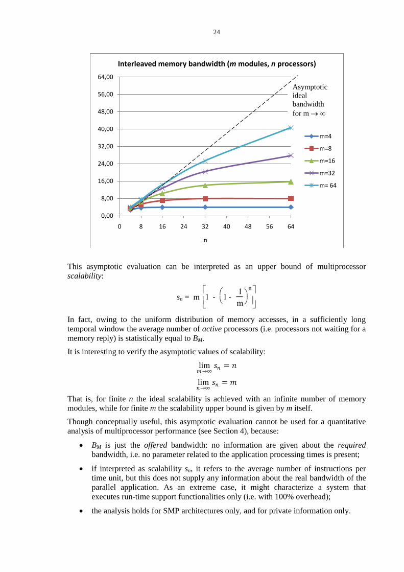
which is graphically shown in the following Figure.
As expected, shared memory conflicts play an important, negative role in multiprocessor
performance, because the memory bandwidth degradation is sensible for high values of n.
(Nevertheless, the absolute values of memory bandwidth are not necessarily so bad: it has
to be remarked that, in long-word or macro-modules based organizations, the bandwidth
values are measured in cache blocks per access time.)
24
This asymptotic evaluation can be interpreted as an upper bound of multiprocessor
scalability:
sn = m 1 - 1 - 1
m
n
In fact, owing to the uniform distribution of memory accesses, in a sufficiently long
temporal window the average number of active processors (i.e. processors not waiting for a
memory reply) is statistically equal to BM.
It is interesting to verify the asymptotic values of scalability:
lim𝑚→∞
𝑠𝑛 = 𝑛
lim𝑛→∞
𝑠𝑛 = 𝑚
That is, for finite n the ideal scalability is achieved with an infinite number of memory
modules, while for finite m the scalability upper bound is given by m itself.
Though conceptually useful, this asymptotic evaluation cannot be used for a quantitative
analysis of multiprocessor performance (see Section 4), because:
BM is just the offered bandwidth: no information are given about the required
bandwidth, i.e. no parameter related to the application processing times is present;
if interpreted as scalability sn, it refers to the average number of instructions per
time unit, but this does not supply any information about the real bandwidth of the
parallel application. As an extreme case, it might characterize a system that
executes run-time support functionalities only (i.e. with 100% overhead);
the analysis holds for SMP architectures only, and for private information only.
0,00
8,00
16,00
24,00
32,00
40,00
48,00
56,00
64,00
0 8 16 24 32 40 48 56 64
n
Interleaved memory bandwidth (m modules, n processors)
m=4
m=8
m=16
m=32
m= 64
Asymptotic
ideal
bandwidth
for m ∞

25
1.3.7 Software lockout
The system congestion is further increased by the so-called software-lockout effect, that is
the effect of busy waiting periods caused by indivisible sequences on shared data
structures, e.g. run-time support data structures.
As it will be studied in Sect. 4, these sequences are typically executed in lock state, i.e.,
mutually exclusive sections enclosed between a lock and an unlock operation. A processor,
which is temporarily blocked to enter a lock section, is in a busy waiting state, thus it can
be considered inactive from the point of view of the computation to be executed.
While the analysis of Sect. 1.3.6 refers to waiting periods in absence of indivisible
sequences (i.e. for sequences containing just one memory access), the software lockout
analysis refers to indivisible sequences containing at least two memory accesses.
A worst-case analysis of the software-lockout problem has been done under the
assumption that the busy waiting times are exponentially distributed.
Let:
L be the average time spent inside a lock section,
E be the average time spent outside lock sections.
The average number of inactive processors is expressed by the following function of n and
of L/E parameter:
If L/E increases (i.e., L increases), the average number of inactive processors increases
very rapidly. In the Figure we can observe that L/E should be at most of the order of 10-2
for limiting the scalability degradation to acceptable values.
Moreover, for a given L/E, a threshold value nc exists, such that for n > nc the average
number of inactive processors grows linearly, i.e. in practice any additional processor over
average number of inactive processors

26
nc is just an inactive one. For values of L/E having order of magnitude greater than 10-2
this
threshold value is rather low. Consequently, in the run-time support design, the lock
section lengths have to be minimized, notably by trying to decompose each lock section
into a number of smaller, independent lock sections, possibly interleaved each other.
Although the above analysis is a worst case one, the software lockout effect might become
a serious problem in parallel applications. Just to prove this assertion, it is worth knowing
that software lockout was the main cause of the commercial failures of some industrial
multiprocessor products which tried to adopt uniprocessor operating systems, like Unix. In
such operating system versions, the L/E ratio is as large as 60% and over, therefore
disappointing scalability values were achieved. In order to correct this conceptual and
technological error, the operating system versions (Unix kernel) for multiprocessors were
completely re-written adopting minimization techniques of lock sections.
1.4 Multicomputers
In this class of MIMD architectures, no memory sharing is physically possible among
processes allocated onto distinct processing nodes. That is, the result of the translation of a
logical address, generated by any processor running on a node Ni, cannot be a physical
address of the main memory belonging to a distinct node Nj. Memory sharing is prevented
at the firmware level, though it could be emulated at a higher level. The only primitive
architectural mechanism for node cooperation is the communication by value, that is the
cooperation via input-output mechanisms and interface units. Interprocess communication
is implemented on top of such mechanism.
Many enabling platforms belong to the multicomputer class: massively parallel processors
(MMP), network computers, clusters of PCs/workstations, multi-clusters, server farms,
data centres, grids, clouds, and so on. The figure in the next page shows clusters belonging
to different technological generations:
27
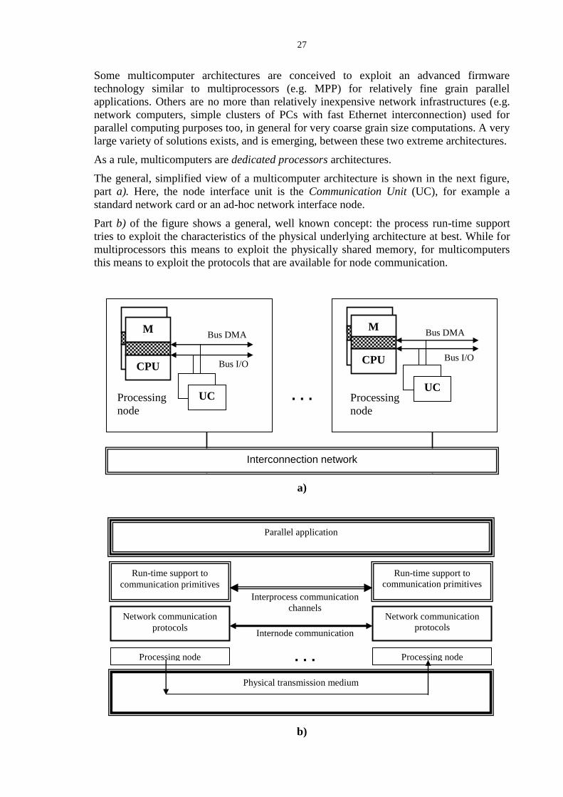
Some multicomputer architectures are conceived to exploit an advanced firmware
technology similar to multiprocessors (e.g. MPP) for relatively fine grain parallel
applications. Others are no more than relatively inexpensive network infrastructures (e.g.
network computers, simple clusters of PCs with fast Ethernet interconnection) used for
parallel computing purposes too, in general for very coarse grain size computations. A very
large variety of solutions exists, and is emerging, between these two extreme architectures.
As a rule, multicomputers are dedicated processors architectures.
The general, simplified view of a multicomputer architecture is shown in the next figure,
part a). Here, the node interface unit is the Communication Unit (UC), for example a
standard network card or an ad-hoc network interface node.
Part b) of the figure shows a general, well known concept: the process run-time support
tries to exploit the characteristics of the physical underlying architecture at best. While for
multiprocessors this means to exploit the physically shared memory, for multicomputers
this means to exploit the protocols that are available for node communication.
a)
b)
. . .
Internode communication
channels
Interprocess communication
channels
Physical transmission medium
Parallel application
Run-time support to
communication primitives
Network communication
protocols
Run-time support to
communication primitives
Network communication
protocols
Processing node Processing node
Interconnection network
. . .
CPU
Processing
node
Bus DMA
Bus I/O
M
CPU
UC
CPU
Processing
node
Bus DMA
Bus I/O
M
CPU
UC

28
In some cases, standard communication protocols. i.e. IP-like, are directly used, at the
expense of a large overhead and performance unpredictability for parallel computations. In
other cases, similarly to multiprocessors, the primitive firmware protocol of the
interconnection network is used, with sensible improvements in bandwidth and latency of
one or more orders of magnitude compared to IP-like protocols, as well as in performance
predictability.
Also for multicomputers, the main peculiar characteristic (i.e. distributed memory) is an
advantage and a disadvantage at the same time:
on one hand, the absence of a shared memory leads to potentially scalable
solutions,
on the other hand, interprocess communication between processes allocated onto
distinct nodes is delayed by the network latency, and possibly by heavy
communication protocols, for long messages (longer than in multiprocessors, where
firmware messages are used for remote memory accesses or short interprocessor
communications).
In other words, phrases like “shared memory is a bottleneck for multiprocessors” and “high
scalability is achieved in distributed memory architectures” are rather simplistic. In both
MIMD architectures the interconnection network congestion problems represent the
dominant issue for performance. In multiprocessors, additional congestion is caused by
memory sharing, however the shorter firmware messages have a positive effect on the
exploitation of network bandwidth.
No simplistic conclusion about the performance comparison of the two MIMD classes is
possible a priori, provided that also the multicomputer systems adopt the primitive
firmware protocol of the interconnection network.
1.5 Multicore/manycore examples
In this Section we apply the MIMD architectures overview to the analysis of some
multicore products considered representatives of the state-of-the art and of some current
trends in this area. The following features will taken into account:
general-purpose vs special-purpose, notably network processors, architectures
homogeneous vs heterogeneous architectures,
SMP vs NUMA shared memory architectures,
low parallelism vs high parallelism architectures.
1.5.1 General-purpose architectures: current, low parallelism chips
Typical members of this class are x86-based chips:
Intel Xeon (Core 2 Duo, Core 2 Quad), Nehalem
AMD Athlon, Opteron quad-core (Barcelona)
Power PC based:
IBM Power 5, 6
IBM Cell

29
UltraSPARC based:
Sun UltraSparc T1, T2
Except IBM Cell, all the mentioned products are homogeneous, shared cache (L2 / L3)
multiprocessors. Figures 1, 2, 3 shows the main characteristics of Intel and AMD
multicores.
Fig. 1: Intel Xeon - SMP
Fig. 2: Intel Nehalem - SMP

30
Fig. 3: AMD Opteron Quad Core - NUMA
SUN Niagara line, UltraSPARC T2 is a SMP, shared L2-cache multiprocessor, with 8
simple, pipelined, in-order cores interconnected by a crossbar, 8 simultaneous threads per
core, each core equipped with one floating point unit.
IBM BlueGene/P is basically a PowerPC 32-bit quad-core, having a NUMA architecture
with 2-dimension mesh interconnection network and automatic cache coherence. Each core
is able to execute 4 simultaneous floating point operations per clock cycle (850 MHz). It is
characterized by a significantly less power consumption (16 W) compared to the over 65
W of x86 quad-core products. This chip is the basic component of the BlueGene MPP
system, extendable to over 75000 quad-core chips (thus, over 290000 cores).
The IBM Cell BE has been one of the first multicore architectures especially developed for
highly parallel, fine grain parallel computations:
31
It can be considered the evolution of uniprocessor Power PC (Processor Element, PPE),
equipped with 8 I/O vectorized coprocessors, towards a heterogeneous NUMA
multiprocessor: that is, the I/O coprocessors have been transformed into general Processing
Cores (Synergistic Processing Element, SPE) with vectorization capabilities:
PPE is superscalar, in-order, with L2-cache accessible by the SPEs. PPE is mainly used as
a master processor for basic operating system and loading tasks, as well as an intelligent
shared memory repository for SPEs.
Each SPE is RISC, 128-bit, pipelined, in-order, with vectorized instructions. The SPE
Local Memory, which is not a cache, is rather small (256 Kb) and must be managed by
program explicitly. The interconnection structure consists in 4 bidirectional Rings, 16
bytes per ring.
It has been experimented that Cell is characterized by a reliable cost model for memory
access and communication. It is now out of market, and it will be replaced by the
WireSpeed processor, described in a subsequent Section.
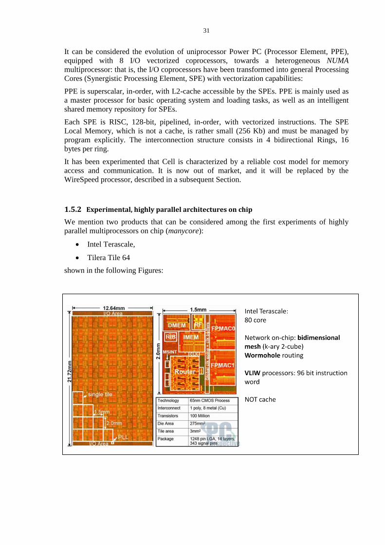
1.5.2 Experimental, highly parallel architectures on chip
We mention two products that can be considered among the first experiments of highly
parallel multiprocessors on chip (manycore):
Intel Terascale,
Tilera Tile 64
shown in the following Figures:
32
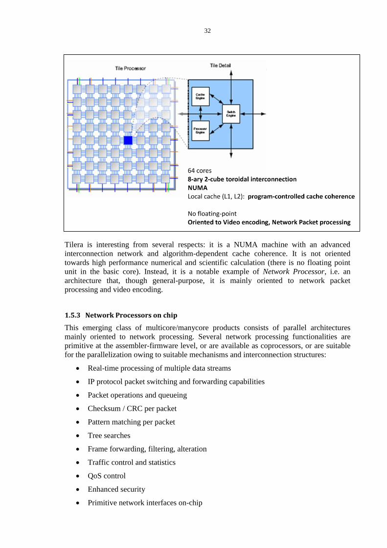
Tilera is interesting from several respects: it is a NUMA machine with an advanced
interconnection network and algorithm-dependent cache coherence. It is not oriented
towards high performance numerical and scientific calculation (there is no floating point
unit in the basic core). Instead, it is a notable example of Network Processor, i.e. an
architecture that, though general-purpose, it is mainly oriented to network packet
processing and video encoding.
1.5.3 Network Processors on chip
This emerging class of multicore/manycore products consists of parallel architectures
mainly oriented to network processing. Several network processing functionalities are
primitive at the assembler-firmware level, or are available as coprocessors, or are suitable
for the parallelization owing to suitable mechanisms and interconnection structures:
Real-time processing of multiple data streams
IP protocol packet switching and forwarding capabilities
Packet operations and queueing
Checksum / CRC per packet
Pattern matching per packet
Tree searches
Frame forwarding, filtering, alteration
Traffic control and statistics
QoS control
Enhanced security
Primitive network interfaces on-chip
33
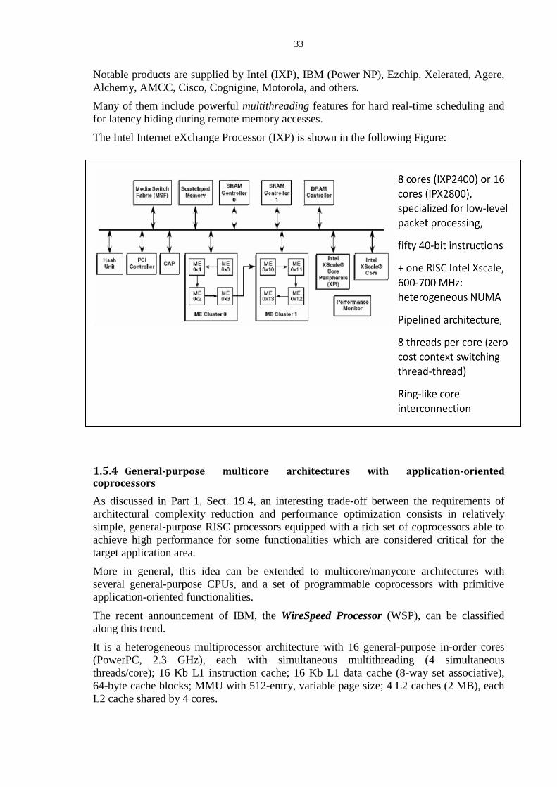
Notable products are supplied by Intel (IXP), IBM (Power NP), Ezchip, Xelerated, Agere,
Alchemy, AMCC, Cisco, Cognigine, Motorola, and others.
Many of them include powerful multithreading features for hard real-time scheduling and
for latency hiding during remote memory accesses.
The Intel Internet eXchange Processor (IXP) is shown in the following Figure:
1.5.4 General-purpose multicore architectures with application-oriented coprocessors
As discussed in Part 1, Sect. 19.4, an interesting trade-off between the requirements of
architectural complexity reduction and performance optimization consists in relatively
simple, general-purpose RISC processors equipped with a rich set of coprocessors able to
achieve high performance for some functionalities which are considered critical for the
target application area.
More in general, this idea can be extended to multicore/manycore architectures with
several general-purpose CPUs, and a set of programmable coprocessors with primitive
application-oriented functionalities.
The recent announcement of IBM, the WireSpeed Processor (WSP), can be classified
along this trend.
It is a heterogeneous multiprocessor architecture with 16 general-purpose in-order cores
(PowerPC, 2.3 GHz), each with simultaneous multithreading (4 simultaneous
threads/core); 16 Kb L1 instruction cache; 16 Kb L1 data cache (8-way set associative),
64-byte cache blocks; MMU with 512-entry, variable page size; 4 L2 caches (2 MB), each
L2 cache shared by 4 cores.
34
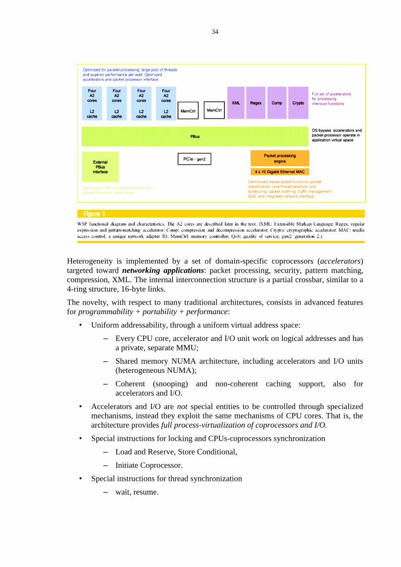
Heterogeneity is implemented by a set of domain-specific coprocessors (accelerators)
targeted toward networking applications: packet processing, security, pattern matching,
compression, XML. The internal interconnection structure is a partial crossbar, similar to a
4-ring structure, 16-byte links.
The novelty, with respect to many traditional architectures, consists in advanced features
for programmability + portability + performance:
• Uniform addressability, through a uniform virtual address space:
– Every CPU core, accelerator and I/O unit work on logical addresses and has
a private, separate MMU;
– Shared memory NUMA architecture, including accelerators and I/O units
(heterogeneous NUMA);
– Coherent (snooping) and non-coherent caching support, also for
accelerators and I/O.
• Accelerators and I/O are not special entities to be controlled through specialized
mechanisms, instead they exploit the same mechanisms of CPU cores. That is, the
architecture provides full process-virtualization of coprocessors and I/O.
• Special instructions for locking and CPUs-coprocessors synchronization
– Load and Reserve, Store Conditional,
– Initiate Coprocessor.
• Special instructions for thread synchronization
– wait, resume.

35
2. Interconnection networks
This Section deals with interconnection networks for any kind of MIMD architecture. We
will see that, though few of them are more suitable for specific architectures, several
networks can be used in both classes of parallel architectures (shared memory
multiprocessors and distributed memory multicomputers), provided that proper
mechanisms are realized in processing nodes and in networks nodes according to the
specific architecture class.
The focus will be on limited degree networks which, with respect to traditional buses and
crossbars, are suitable for scalable, highly parallel architectures. In an architecture based
on limited degree networks, a processing node is directly connected to a small subset of
nodes, or it is indirectly connected to any other node through an intermediate path of
switching nodes. As a rule, these networks provide some degree of symmetry, for
modularity, efficiency and cost-model predictability reasons.
2.1 Network topologies
For clarity and completeness of presentation, this Section contains a repetition of Sect. 1.2.
A first characteristic of interconnection networks consists in the following distinction:
direct, or static, networks,
indirect, or dynamic, networks.
In a direct network, point to point dedicated links connect the processing nodes in some
fixed topology. Of course, messages can be routed to any processing node which is not
directly connected. Each network node, also called switch node, is connected to one and
only one processing node, possibly through the node interface unit (logically, W is not
necessary if the network node plays this role too). Notable examples of limited-degree
direct networks for parallel architectures are:
Rings,
Meshes and Tori (toroidal meshes),
Cubes (k-ary n-cubes),
shown in figure 1.
In an indirect network, processing nodes are not directly connected; they communicate
through intermediate switch nodes, or simply switches, each of which has a limited number
of neighbors. In general, more than one switch is used to establish a communication path
between any pair of processing nodes. These structures are also denoted as dynamic
networks, since they allow the interconnection pattern among the network nodes to be
varied dynamically through the proper cooperation of switching units. Buses and crossbars
are indirect networks at the possible extremes. Notable examples of limited-degree indirect
networks for parallel architectures are:
Multistage networks,
Butterflies (k-ary n-fly),
Trees and Fat Trees,
shown in the figure 2.
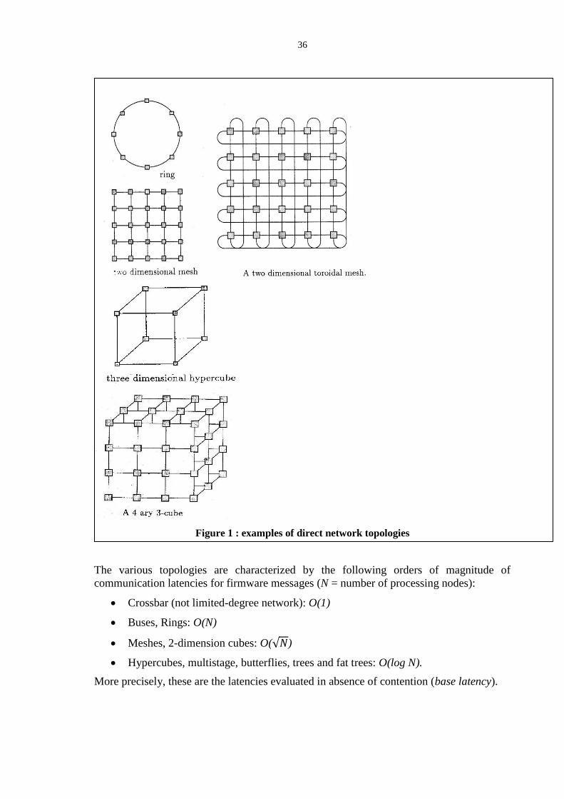
36
Figure 1 : examples of direct network topologies
The various topologies are characterized by the following orders of magnitude of
communication latencies for firmware messages (N = number of processing nodes):
Crossbar (not limited-degree network): O(1)
Buses, Rings: O(N)
Meshes, 2-dimension cubes: O( 𝑁)
Hypercubes, multistage, butterflies, trees and fat trees: O(log N).
More precisely, these are the latencies evaluated in absence of contention (base latency).

37
Figure 2: examples of indirect network topologies
N
0
N
1
N
2
N
3
N
4
N
5
N
6
N
7

38
2.2 Properties of interconnection networks
Node degree
This property is measured by the number of links incident in a network node. The
definition can take into account bidirectional links, e.g. a pair of input and output
unidirectional links are considered a single bidirectional link for the evaluation of node
degree.
This metric reflects the cost of a node, which is mainly due to the pin-count measure; thus,
in a limited degree network, it should be kept as small as possible.
Distance measures
Communication between two nodes that are not directly connected must take place by
routing mechanisms: through other network nodes in a direct network, or through
intermediate switches in an indirect one. Although the actual path depends upon the
routing algorithm, for the moment being we consider the shortest path as a topological
characteristic.
The network diameter is defined as the maximum length of the shortest communication
paths between all possible pairs of nodes.
Although the diameter is useful in comparing two topologies with identical node degree, it
may be not always indicative of the actual performance. In practice, it is more important to
measure the “distance” traveled by an “average” message. The mean internode distance, or
average distance, is the average length of all the paths traveled by messages in the
network. While the diameter depends only on the network topology, the distance also
depends on the mapping of the cooperating processing modules and their communication
patterns. Thus, for an arbitrary message distribution:
𝑎𝑣𝑒𝑟𝑎𝑔𝑒 𝑑𝑖𝑠𝑡𝑎𝑛𝑐𝑒 = 𝑖 ∗ 𝑝(𝑖)
𝑑
𝑖=1
where d is the diameter, and p(i) is the probability of messages that travel a distance i.
We say that an application exploits communication locality if there is an upper bound b
such that p(j) = 0 j b. Communication locality is a desirable feature concerning the
parallel application mapping. We will see that there are some network topologies which are
locality sensitive, i.e. the communication latency depends heavily on the average distance,
while for other notable networks the communication latency tends to increase slowly with
the distance, at least for message traffic under a certain network utilization factor.
Unless specific assumptions about the parallel computation mapping are done, we assume
the uniform distribution for p(i), i.e. each node send messages to any other node with equal
probability. In this case:
𝑎𝑣𝑒𝑟𝑎𝑔𝑒 𝑑𝑖𝑠𝑡𝑎𝑛𝑐𝑒 = 1
𝑁 𝑖 ∗ 𝑛(𝑖)
𝑑
𝑖=1
where N is the number of processing nodes, and n(i) is the number of nodes at a distance i
from a given node.
Some interesting limited degree networks have an important feature: their average distance
is logarithmic in the number of nodes
39
average distance = O(log N)
Analogously to what happens in algorithm theory, a logarithmic distance is a very good
result with respect to the best distance as possible, i.e. with respect to a constant O(1)
distance, which is typical of the too expensive non-limited degree crossbar networks.
Logarithmic networks are hypercubes (k-ary n-cubes with high n), multistage networks (k-
ary n-flies), trees and fat trees.
Other limited degree networks, notably two dimensional meshes and k-ary n-cubes with
low n, are characterized by a distance which, as order of magnitude, is higher compared to
the logarithmic ones:
𝑎𝑣𝑒𝑟𝑎𝑔𝑒 𝑑𝑖𝑠𝑡𝑎𝑛𝑐𝑒 = 𝑁𝑛
However, we will see that, according to the value of the multiplicative constant, some
square-root (or cubic-root) networks have a better latency than some logarithmic networks
of the some class (notably, low n k-ary n-cubes compared to high n k-ary n-cubes).
Of course, limited degree networks such as buses are characterized by a distance which is
not acceptable for highly parallel systems:
average distance = O(N)
Other limited degree networks such as rings have this characteristic.
Another performance metric is the average traffic density on a link, measured by the link
offered bandwidth (the mean number of messages carried by the link in a time unit). The
network offered bandwidth measures the so-called network capacity, which, as usually,
depends on the bandwidth of the bottleneck links (i.e. the average traffic density of the
bottleneck links). For example, in a binary tree the message density increases along a path
from any leaf to the root under uniform traffic; the fat tree network is conceived in order to
properly increasing the link bandwidth as the distance increases.
Bisection width
This important property is used to evaluate the link and/or wires density and the network
connectivity degree. It is also useful in estimating the area required for a VLSI
implementation of the network.
Considering the network as a graph, the bisection width is defined as the minimum number
of edges that must be removed to partition the original graph of N vertices into two
subgraphs of N/2 vertices each (if N is odd, two subgraphs of (N+1)/2 and (N-1)/2
respectively).
For example, the bisection width of a two dimensional mesh with N nodes is 𝑁. For a
binary n-dimension cube (N = 2n nodes) the bisection width is N/2. This shows the dense
connectivity of the hypercubes compared to the meshes.
Network latency
The network latency is measured as the actual time latency needed to establish a
communication through the network between the source and the destination node.
The base network latency is defined as the network latency measured without contention.
Informally, this corresponds to the situation in which no link conflict between any pair of

40
messages occurs. Formally, this means that the utilization factors of each network link
(considered as a server in a client-server queueing system) are equal to zero (network = 0).
The base latency is not a function of message traffic. It is just a function of architectural
characteristics:
switch delay (switching unit service time),
wire delay (Ttr, wire transmission latency),
network distance,
message length,
routing strategy,
flow control strategy.
The base latency is an ideal latency evaluation, taking into account only the architectural
features of a communication network.
The effective latency, or under-load latency, takes into account the contention, i.e. link
conflict situations. Formally, we evaluate the network according to a queueing model,
where each network link is a server in a client-server queueing system (Part 1, Section 16).
The network load, or network traffic, is measured as the response time of the servers, thus
as a function of
the network utilization factor network,
the service time tS and interarrival time tA distributions,
the network base latency itself, i.e the server latency LS.
From a qualitative viewpoint, we have the known function shape:
2.3 Buses and crossbars
Buses and crossbars represent the two extreme solutions to interconnection networks. Their
principle is illustrated in the following figure.
The highest-end structure is the fully interconnected crossbar, while the bus is the most
elementary limited-degree network.
1 0
Under-load
network latency
Base
network latency
network
critical

41
Buses are the most common interconnection networks for uniprocessor systems (I/O
subsystem, including DMA) and for the first-generation low parallelism multiprocessors.
Though being limited degree structures (by definition), they are not suitable for highly
parallel systems, because of their linear distance and latency, their limited parallelism (at
most one message can be transmitted at the time), thus limited scalability, as well as
limited availability in case of failures.
The extension to multiple buses networks, also called partial configuration or partial
crossbar, has been adopted in several systems to partially overcome the mentioned
drawbacks.
A crossbar, shown in the following figure in the classic example of a shared memory SMP
multiprocessor, is a fully interconnected network:
In the figure, a switching unit is placed at each of the n2 crossing point of the horizontal
and vertical lines.
Simplified bus
scheme
Simplified crossbar
scheme
42
A crossbar is not a limited degree network: it is of O(N2) complexity in terms of hardware
resources (switches) and area, thus it can be used only in limited parallelism systems or
subsystems, including chips with a small number of cores. In these cases, the distance and
latency are constant, i.e. the best as possible.
It may be interesting to define networks built around a large number of limited degree
switching units, each of which exploits an internal small crossbar structure.
Moreover, crossbar can be effectively emulated by k-ary n-fly networks and fat trees, as
studied in subsequent Sections.
2.4 Rings, multi-rings, meshes and tori
In the version with bidirectional links, a ring with N nodes is a simple direct network, with
node degree equal to 2 (one bidirectional input link and one bidirectional output link per
node), diameter N/2 and average distance N/4.
Though not suitable for highly parallel systems and having limited availability in case of
failures, rings have many interesting properties that can be exploited to implement
sophisticated functionalities, such as multicast communications and cache coherence
protocols. For this reason, and owing to its simplicity, it is adopted as a basis in some
multicore chips, notably in multi-ring version.
Similarly, bidimensional meshes (node degree equal to 4), and their toroidal versions with
wraparound connections, are adopted in several MPP machines and in some emerging
multicore/manycore chips. As said, they have O( 𝑁) distance and base latency.
At a first sight, many simple parallel algorithms can be mapped directly onto mesh-based
architectures, for example image processing, matrix computations, numerical solutions of
differential equations (convolutions), and computational geometry. However, as we know
according to Part 1 methodology, often the parallel paradigms for these applications need
additional channels that are not mapped directly onto mesh structures, e.g. scatter, gather,
multicast, reduce, stencils.
More in general, looking for a relationship between parallel computation structure and
network structure is not meaningful, except for some special-purpose machines. Instead,
we are interested in studying limited degree network topologies with interesting properties
for a large variety of parallel paradigms and their compositions. Similarly, attempts to
reduce the mesh diameter by introducing additional links (e.g. a global bus, or rows and
columns of busses) are not to be considered meaningful for future high performance
systems, because they tend to specialize the architecture towards particular applications or
algorithms.
Rings, meshes and their variants, as well as hypercubes, are particular cases of the general
k-ary n-cube class, which is studied in a subsequent section.
2.5 Routing and flow control strategies
It is out of the scope of this course to give a complete treatment of routing strategies and
algorithms, for which a rich specialized literature exists. In this Section, we focus on the
main issues of interest about routing and flow control for highly parallel architectures.

43
A general consideration has to be stated first: though the basic concepts are common to any
networking infrastructure, interconnection networks for parallel architectures are able to
execute the routing and flow control strategies directly at the firmware level, i.e. according
to efficient and performance-predictable primitive firmware protocols. This avoids the
large overhead and performance unpredictability, which are typical of other networks,
notably with IP or similar protocols. However, some commercial networks are available in
double version: with firmware-primitive protocol and with IP protocol; the latter version
allows the application designer to reuse existing codes that employ IP protocols, unless a
much higher and predictable performance is needed (in this case, the firmware-primitive
version must be adopted).
2.5.1 Routing: path setup and path selection
The following figure shows a possible taxonomy of communication methods employed in
interconnection networks:
Usually, in parallel architectures, the path setup, or path configuration, is determined
dynamically on demand. This can be done according to the classical methods of packet
switching, or also message switching for short messages (e.g. for remote memory
accesses), while circuit switching is rarely adopted.
The routing path selection is defined in terms of a relation R and a function F, defined on
the set of physical links L and on the set of processing nodes N:
44
R L x N x L
F: Perm(L) x L
Given the current link l L and the destination node n N, the routing relation R
identifies a set of permissible links Perm(L) L, that can be used in the next step on the
route. R is a relation, because there can be several alternative paths to reach the
destination. At each step of the route, the function F selects one link l Perm(L), possibly
exploiting some additional information on the state of the network, for example current
link/node load and availability.
The simplest routing approach is the deterministic one, in which the route is fully
established by the source and destination addresses (identifiers). Though simple, this
approach is unable to adapt the network to dynamic conditions, such as congestion or
failures and, in general, communication patterns.
Adaptive routing, which has been a notable area in ICT research and technology, aims to
provide network performance that is less sensitive to the communication pattern.
As shown in the following simple example, in a deterministic routing strategy several
message can cross the same “hot” node (in black), even if there are some alternative paths
to handle the communication pattern; while an adaptive routing strategy can route distinct
messages along distinct paths.
Often, simple and efficient firmware mechanisms are sufficient to collect information on
the state of the network in an adaptive routing strategy, notably the “ack” signals of the
output interfaces in a network node, possibly associated to firmware time-outs and history
information. Moreover, the parallel paradigm constraints could be able to supply useful
information about the communication pattern load.
A minimal adaptive routing limits the path selection to the shortest paths between any
given pair (source, destination). With a non-minimal routing algorithm, the selected path
may not always be a shortest path.
Adaptive routing is also able to better support deadlock avoidance strategies (not studied
here).

45
2.5.2 Flow control and wormhole routing
In general, the term flow control denotes the set of techniques to manage the network
resources, notably links, switch nodes, and buffering capacity.
In a store and forward strategy, at each intermediate node a packet (or a single-packet
message) must be entirely buffered before being forwarded onto the proper output link, if
and when available.
In any flow control strategy, the packet is the unit of routing, i.e. all the words belonging to
the same packet must travel exactly the same path. In a packet switching path setup
strategy, distinct packets of the same message can be routed independently onto distinct
paths, thus exploiting potential parallelism at the packet grain size level.
In interconnection networks for parallel architectures, an additional source of parallelism
can be efficiently exploited: in the so-called wormhole flow control, each single packet is
further decomposed into smaller units, called flits, for example one words or few bytes,
often coinciding with the link width. All the flits of the same packet follow the same route
(as said above, the packet is the unit of routing), however flits are considered as streams
elements in a pipelined transmission. That is, the flits of the same packet are not entirely
buffered before being routed, instead the buffering unit is the flit: as soon as a flit is
received, it is forwarded onto the output link selected by the packet routing strategy, and
the next flit is immediately used, or the flit waits in the network/switching node.
In this way, we are able to achieve the typical completion time benefits of a pipeline
implementation compared to the sequential implementation (store and forward), provided
that the switching node bandwidth per flit is high enough, as it holds in parallel
architectures in which the routing and flow control strategies are implemented at the very
primitive firmware level (one clock cycle). On the contrary, in a typical IP network, the
routing and flow control service time is too high to be able to exploit a wormhole strategy
effectively.
Moreover, owing to the minimization of the buffering area, the wormhole technique is of
special interest in the implementation of networks on chip.
As a rule, the first flit of a packet is the packet header containing the routing information,
notably (source identifier, destination identifier) and packet length. Exploiting such
information, the switching node executes the routing strategy and establishes the output
link, so that all the other flits of the same packet will be forwarded onto this link, when
available. In case of a temporary block of the output link (e.g. the ack is delayed), the
packet buffering is distributed backward in the preceding network units along the path.
In the virtual cut through variant, the pipeline transmission is equally applied, but, in case
of a blocking situation, all the “worm” flits are received by, and buffered into, the blocked
switching node, as in the store and forward flow control.
2.5.3 Switching nodes for wormhole networks
The structure of a wormhole network switching node, with node degree equal to four, is
illustrated in the following figure:
The behavior is characterized as follows:
all communications with the neighbor switching nodes are performed by
asynchronous, level-transition interfaces with standard rdy-ack synchronization;

46
each switching node SWi is able to execute several unidirectional communications in
parallel, for example by decomposing the node into two independent sub-units, SWi1
and SWi2, one for each network direction;
each sub-unit is able to execute the following actions in a single clock cycle:
1. according to the header flit information of both the input messages (if both are
present), determines their respective output interfaces: if they are distinct, both flits
are routed in parallel, otherwise one is selected and the other header flit waits;
2. for each routed message, a loop controlled by the message length is executed,
during which the subsequent flits are sent onto the already selected interface;
3. go to step 1, taking into account that, if one of the message transmission is still on-
going, the other input interface is continuously tested too, in order to verify the
possible presence of a new message. If so, this message can be routed immediately,
provided that it uses the free interface, otherwise the header flit waits.
2.5.4 Communication latency of structures with pipelined flow control
In many cases, parallel architectures exploit forms of pipelined system-wide
communication. For example, streams of data blocks read in parallel from a high
bandwidth memory (interleaved macro-module, or long-word module), traveling through
processing node interface units, and, of course, through wormhole-based switches.
In other words, the pipelined transmission is applied to paths that include, but are not
limited to, wormhole network sections: in this way, the bandwidths of the processing and
of the switching units are balanced through the application of a fine grain pipeline
paradigm.
Let any unit along a pipelined path have a service time equal to and any link a
transmission latency equal to Ttr. The typical scheme of a pipeline, in which the first stage
SWi
SWi1
Routing
and
flow control
OUT11 IN11
OUT12 IN12
SWi2
Routing
and
flow control
IN21 OUT21
IN22 OUT22

47
generates the stream and the final one collects the stream elements, is shown in the
following figure:
Let d the whole number of pipelined units and m the stream length (in the example, d = 4,
m = 5). The latency is given by:
Tlat-pipe = (m – 1) 2 ( + Ttr) + (d – 1) ( + Ttr) = (2m + d – 3) ( + Ttr)
The final clock cycle is spent in processing actions, thus has not been counted in the
latency expression. Let:
thop = + Ttr
called hop latency (i.e., the latency of a switch+link section). Thus:
Tlat-pipe = (2m + d – 3) thop
This formula can be easily generalized in the case of different clock cycles or service times
greater than a single clock cycle.
2.6 k-ary n-cube networks
2.6.1 Characteristics and routing
This class generalizes rings, meshes, tori and hypercubes. k-ary n-cube networks are
especially suitable for NUMA multiprocessors and for multicomputers, as well as SIMD
coprocessors and other special-purpose machines.
The following figure shows how higher dimension cubes can be recursively built starting
from lower dimension ones with the same arity k. The number of nodes is given by:
𝑁 = 𝑘𝑛
where n is the cube dimension. The node degree is 2n. For symmetry reasons, toroidal
structures with wrap-around connections are often provided, so that no boundary nodes
exist.
A deterministic routing strategy exploits one of the possible shortest paths between source
and destination nodes. The message header includes the routing information: source and
destination node identifiers expressed as coordinates in the n-dimension space:
message header = (source node identifier, destination node identifier, message length,
message type)
(m – 1) 2 ( + Ttr) (d – 1) ( + Ttr)

48
The simple deterministic routing function is of dimensional kind. For example, for n = 2,
let (Xs, Ys) be the source node coordinates and (Xd, Yd) the destination node coordinates.
The first dimension is followed until the node with coordinates (Xd, Ys) is reached, then
the second dimension is followed until the destination node (Xd, Yd) is reached. This
algorithm can be easily generalized to any n.
Other non deterministic routing algorithms can be the adaptive ones (the minimal adaptive
algorithm is still a dimensional one, consisting in selecting one of the paths belonging to
the shortest paths set).
2.6.2 Cost model: base latency under physical constraints
From the point of view of the cost model, it is useful to distinguish between low
dimension cubes (n = 2, 3 dimension meshes) and high dimension cubes, typically the
binary hypercube with k = 2. For example, a system with N = 256 nodes can be
implemented as a 2-ary 8-cube (8-dimension binary hypercube), or as 16-ary 2-cube (2-
dimension mesh with 16 nodes per side).
The node distance is of order O(k n). For a given number of nodes N,
4-ary 2-cube
4-ary 1-cube
bidirectional link.
In a toroidal structure, a wrap-around
link, so each node has 2 neighbors. network node
4-ary 3-cube

49
for relatively low dimension networks, k dominates, thus the average distance is
O( 𝑁𝑛
),
for relatively high dimension networks, n dominates, thus the average distance is
O(𝑙𝑜𝑔𝑘N).
Despite the different orders of magnitude, the comparison between the high dimension
solution (e.g. 2-ary 8-cube) and the low dimension one (e.g. 8-ary 2-cube) is not so
obvious, since the multiplicative constant value in the latency expression plays a very
important role.
This evaluation has been studied by Dally and Agarwal for networks with wormhole flow
control, under physical constraints. The following figure shows the base latency as a
function of the network dimension n, considering the wire delay (Ttr, wire transmission
latency) normalized with respect to the wire delay of a two dimensional cube, assuming a
linear model for the wire delay.
In this figure, constraints about the bisection width and the pin count are not considered.
This is a quite optimistic evaluation for the high dimensional cubes, for which an
unbounded number of network node connections have been assumed. This figure focuses
on the limits of signal propagation alone. This physical limitation tends to favor low
dimensional networks (n = 2, 3). For example, for a 4096 node system, the binary
hypercube has a base latency three time higher than the corresponding three dimensional
cubes.
Embedding a logical topology into the physical word poses the problem of wire density. As
seen, a measure of wire density is the bisection width. The bisection width for a torus
connected k-ary n-cube is
𝑏𝑖𝑠𝑒𝑐𝑡𝑖𝑜𝑛 𝑤𝑖𝑑𝑡 = 2 𝑊 𝑁
𝑘
where W is the link width in bits. For example, the bisection width is 2W in a ring, 2Wk in
a mesh, and WN in a binary hypercube.

50
A meaningful evaluation is given by keeping the bisection width constant, normalizing its
value to N, which is equal to the bisection width of a binary hypercube with serial links.
The result is shown in the following figure:
The fixed bisection width constraints is often considered too restrictive, because it
indicates a cost factor more than a physical limitation.
A more realistic bound is provided by the pin count of each chip. In this case, we can keep
constant the number of pins to 128 binary wires per node (not counting rdy-ack and ground
lines). The impact on the base network latency is shown in the following figure:
In conclusion, the low dimensional cubes, which are able to exploit much wider links with
the same link and chip cost, outperform high dimensional ones.
51
2.7 k-ary n-fly networks
2.7.1 Basic characteristics
The following figure shows an indirect, multistage network modeled as a butterfly of ariety
k and dimension n (shortly, k-ary n-fly), in this example with k = 2 and n = 3.
It connects N processing nodes (C) with N processing nodes (S), in general of different
kinds, where
𝑁 = 𝑘𝑛
For example, C nodes are CPUs and S nodes are shared memory modules of a SMP
multiprocessor, which is the most notable example of architecture using k-ary n-fly
networks, along with shared memory SIMD machines.
The node degree is equal to 2k.
The distance, coinciding with the diameter, is constant and equal to the dimension n. Thus,
the base latency is proportional to n, that is a k-ary n-fly is a logarithmic network:
base latency = O(n) = O(log N)
A unique shortest path, of length n, connects any C (or S) node to any S (or C) node.
Other multistage networks (Omega, Benes, etc) can be modeled as k-ary n-flies in terms of
interconnection and communication properties.
n = 3
C0
C1
C2
C3
C4
C5
C6
C7
S0
S1
S2
S3
S4
S5
S6
S7
k = 2
Switch unit Processing node Processing node

52
2.7.2 Formalization of k-ary n-fly networks
In order to give a more formal definition of this structure and its properties, let us refer to a
binary butterfly (2-ary n-fly). The treatment can be easily extended to any ariety k.
A binary butterfly
connects N = 2n processing nodes to N = 2
n distinct processing nodes through n
levels of switch nodes;
each level contains N/2 switch nodes;
the two processing node sets are connected, two by two, to the first and to the
last level of switch nodes.
The number of switch nodes and of links is, respectively:
𝑛 2𝑛−1
(𝑛 − 1) 2𝑛
Therefore, as order of magnitude, a butterfly is able to connect N to N processing nodes
with
O(N logN)
switch nodes and links, with an important saving compared to a O(N2) fully interconnected
crossbar.
It may be interesting to notice the analogy, in the area of signal processing, of the Fast Fourier
Transform (FFT) with respect to the Discrete Fourier Transform (DFT). The FFT algorithm has
exactly the binary butterfly topology, and reduces the complexity of DFT from O(N2) to O(N logN),
where N is the amount of complex numbers to which the algorithm is applied. Programmed
according to the data-parallel paradigm, FFT is a static-variable stencil computation which, with N
virtual processors, is executed in log N steps, where, at i-th step, the stencil pattern is exactly
determined by the topology of the i-th level.
The following connectivity rule holds:
each switch node is defined by the coordinates (i, j), with
o i is the row identifier: 0 ≤ i ≤ 2n – 1,
o j is the column (or level) identifier: 0 ≤ j ≤ n – 1;
the generic switch node (i, j), with 0 ≤ j ≤ n – 2, is connected to two switch
nodes:
o (i, j + 1), through the so-called “straight link”,
o (k, j + 1), through the so-called “oblique link”, where k is such that
𝑎𝑏𝑠 𝑘 − 𝑖 = 2𝑛−𝑗−2
In other words, the binary representation of k differs from the binary
representation of i in only the j-th bit starting from the most significant.
The recursive construction of a binary butterfly is defined as follows:
for n = 1, the butterfly consists of just one switch node with two input links and
two output links;
given the n dimensional butterfly, the (n+1) dimensional butterfly is obtained
by applying the following steps:

53
i. two n dimensional butterflies, topologically placed one over the other,
represent the n final levels, each of 2n switch nodes;
ii. the first level, of 2n switch nodes, is added at the left;
iii. the first level nodes are connected to the second level nodes by applying
the connectivity rule, so achieving the full reachability of the two
processing nodes sets.
An n dimensional binary butterfly, with n > 1, is mapped onto a (n-1) dimensional binary
hypercube (2-ary (n-1)-cube): this is achieved by merging all the butterfly nodes of the
same row into one hypercube node, which is identified by the same binary representation
of such row.
2.7.3 Deterministic routing algorithm for k-ary n-fly networks
The following routing algorithm derives from the above properties, and from the
connectivity rule in particular. It applies to both network directions.
Let us consider a binary butterfly (k = 2), whose switch nodes are modeled as belonging to
a matrix with N/k rows and n columns. Each processing node, Ci and Sj, is identified by a
unique natural number represented by n bits. For example let C3 = (011) the source node
and S6 = (110) the destination node. As usually, any message header contains the routing
information consisting of such source and destination node identifiers.
Initially, the message is delivered from the source node to the directly connected switch
node; for example, from C3 to the switch node on the second row and first column. Now
the algorithm follows n steps, corresponding to the network levels. During the i-th step, the
switch node compares the i-th bit of the source and destination identifiers, starting from the
most significant bit. If such i-th bits are equal, then the message is routed onto the straight
link, otherwise onto the oblique link. In the example, the oblique link at the first step, and
the straight link at the second step. The last step is executed by the switch node connected
to the destination node, according to the value of the least significant bit of the destination
identifier (in the example, to the first processing node).
For a Sj source and a Ci destination, the binary representation of identifiers is considered in
reverse order, starting from the second least significant bit. For example, if S6 is the source
and C3 the destination, the first link is straight and the second oblique. The least significant
bit of the destination identifier is used for the final step delivery.
The algorithm is generalized for any ariety k, by considering the k-base representation of
processing node identifiers. At each step, the difference between the source identifier digit
and the destination identifier one is used to uniquely identify the interface onto which the
message is routed.
As for the other networks, non-minimal adaptive routing strategies, i.e. not exploiting the
shortest paths, can be used.
In the next Sections, performance measures for k-ay n-fly networks will be given as
evaluations of generalized fat trees: network structures that basically exploit k-ary n-flyes
to build high bandwidth trees.

54
2.8 Fat Trees
2.8.1 Channel capacity: from trees to fat trees
A tree-structured network can be used as an indirect networks for interconnecting nodes of
the same kinds, notably in a NUMA multiprocessor for both the processor-memory and the
processor-processor structures (thus, unified in the same network), or in a multicomputer,
or in a SMP multiprocessor for the processor-processor structure if distinct from the
processor-memory one.
Communications occur between leaves, where the processing nodes are located/connected,
while all the other nodes, including the root, are switch nodes.
The deterministic routing algorithm is relatively easy, since there is a unique minimal path
between a pair of processing nodes (i, j): a message sent from i goes up the internal
switches until it finds the nearest common ancestor and then down to j.
The base latency is logarithmic. However, for a “normal” tree, latency and bandwidth
under traffic are penalized by the relatively high utilization factor of switch nodes and links
(high conflict rate).
The solution for tree-structured indirect networks is the so-called fat tree:
With respect to a “normal” tree, in a fat tree the link transmission bandwidth, or channel
capacity, increases gradually from the leaves to the root, in order to compensate the
increasing congestion probability. In the figure the typical structure, in which the channel
capacity doubles at each level, is shown. It is responsibility of the routing and flow control
strategy to select one of the output wires to evenly distribute the messages and to minimize
congestion. As consequence, the bandwidth is much greater than the inverse of service
time of a pair switch+link.
2.8.2 Average distance
The average distance, which impacts on the base latency evaluation, is the same for a
normal tree and for a fat tree (instead, the under-load latency is very different).
Under the uniform distribution assumption, the average path length in a binary tree with 2n
leaves is given by:
N0 N1 N2 N3 N4 N5 N6 N7
Network
switch nodes Processing
node
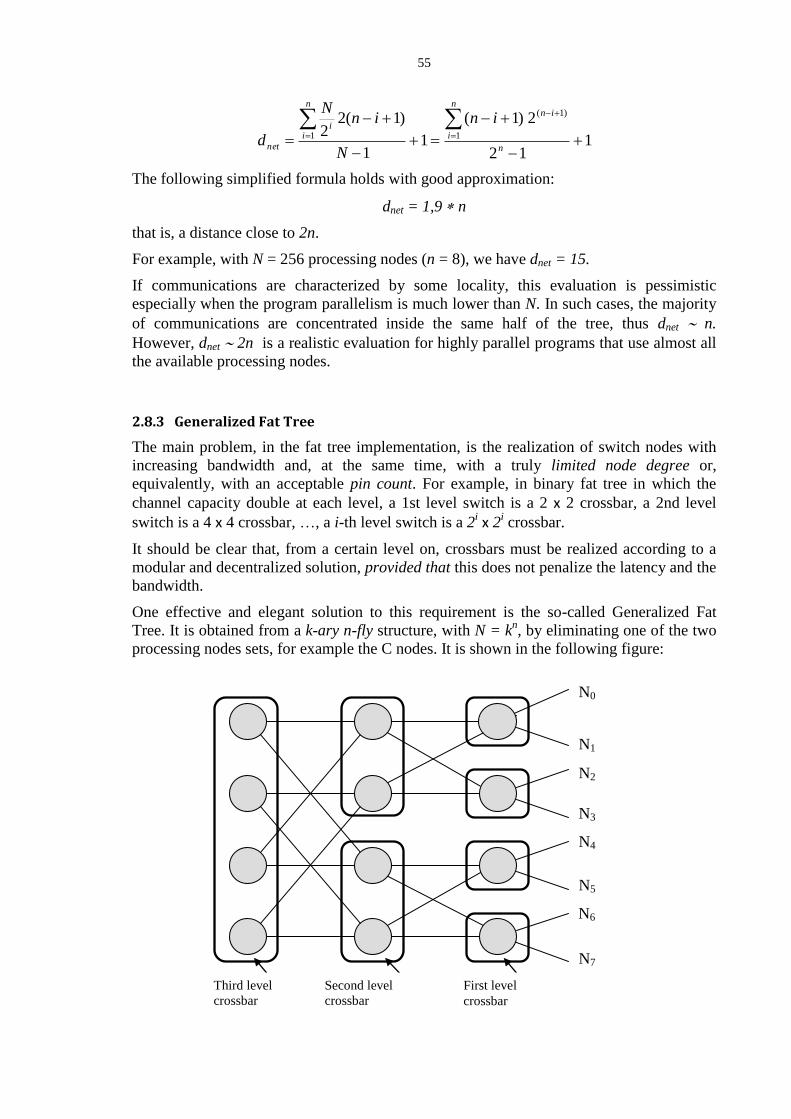
55
112
2)1(
11
)1(22 1
)1(
1
n
n
i
inn
ii
net
in
N
inN
d
The following simplified formula holds with good approximation:
dnet = 1,9 n
that is, a distance close to 2n.
For example, with N = 256 processing nodes (n = 8), we have dnet = 15.
If communications are characterized by some locality, this evaluation is pessimistic
especially when the program parallelism is much lower than N. In such cases, the majority
of communications are concentrated inside the same half of the tree, thus dnet n.
However, dnet 2n is a realistic evaluation for highly parallel programs that use almost all
the available processing nodes.
2.8.3 Generalized Fat Tree
The main problem, in the fat tree implementation, is the realization of switch nodes with
increasing bandwidth and, at the same time, with a truly limited node degree or,
equivalently, with an acceptable pin count. For example, in binary fat tree in which the
channel capacity double at each level, a 1st level switch is a 2 x 2 crossbar, a 2nd level
switch is a 4 x 4 crossbar, …, a i-th level switch is a 2i x 2
i crossbar.
It should be clear that, from a certain level on, crossbars must be realized according to a
modular and decentralized solution, provided that this does not penalize the latency and the
bandwidth.
One effective and elegant solution to this requirement is the so-called Generalized Fat
Tree. It is obtained from a k-ary n-fly structure, with N = kn, by eliminating one of the two
processing nodes sets, for example the C nodes. It is shown in the following figure:
N0
N1
N2
N3
N4
N5
N6
N7
Third level
crossbar
First level
crossbar
Second level
crossbar

56
At each fat tree level, the crossbar switch is realized by a proper number of butterfly
switches operating in parallel without conflicts.
A minimal adaptive routing can be realized according to the butterfly properties, in order
to minimize the conflict probability (the utilization factor), thus with good values of
bandwidth and under-load latency. In practice, in a parallel architecture with Generalized
Fat Tree network, as a first approximation we can neglect the network conflicts with
respect to the conflicts generated at the target shared memory module or destination node.
In other words, the critical utilization factor of a Generalized Fat Tree is relatively high
and the cost model is quite stable for different communication patterns.
Moreover, the Generalized Fat Tree is interesting for its flexibility too. That is, it can be
used as a fat tree (for N processing node with distance 2n) and as a butterfly (for 2N
processing node with distance n) at the same time, according to different message types,
provided that the switch nodes implement both routing strategies. For example, in a SMP
multiprocessor, the same network works for both processor-memory and for processor-
processor communications.
57
3. Cost models for MIMD architectures
In this Section we apply the concepts and techniques on interconnection networks to
evaluate the shared memory access latency for multiprocessor architectures and the inter-
node latency in multicomputer architectures. Analytical cost models will be developed for
the base latency and the under-load latency, in the latter case using queueing system
theory. These evaluations are supported or integrated with experimental and simulation
data.
As said in the previous Section, the same type of interconnection networks can be used in
both a multiprocessor and a multicomputer: there are few basic differences in the type of
traffic handled in the two architectures, as well as in the performance requirements placed
on them. It is worth remembering the distinction between messages at different levels:
firmware messages and inter-process messages (in a message passing cooperation model).
The run-time support of inter-process communications makes use of some firmware
messages crossing the interconnection network:
a) in a multiprocessor, they are mainly remote memory access requests and replies,
and possibly explicit inter-processor communications for scheduling and processor
synchronization purposes. Thus, the traffic handled in a shared memory
multiprocessor consists of relatively small blocks of data in a single packet, i.e.
typically a cache block, or few words for access requests and/or explicit inter-
processor communications;
b) in a multicomputer, generally one of the firmware messages, organized in more
packets, is used for implementing the transmission of the true inter-process
message, enriched by an header and some other utility information of the run-time
support. Moreover, there are further firmware messages for synchronization and
scheduling purposes. Therefore, the length of a firmware message generated in a
multicomputer can vary over a wide range and, on the average, is much larger than
the length in a multiprocessor.
Also, the interconnection network in a multiprocessor must have low latency to keep the
memory access time reasonable, while multicomputers can generally tolerate higher
network latencies.
3.1 Shared memory access latency in multiprocessors
3.1.1 Firmware messages in multiprocessor interconnection networks
To refer to a concrete case, let us assume the following architectural characteristics:
NUMA architecture;
all-cached architecture;
N = 256 processing nodes;
Generalized Fat Tree based on a 2-ary 8-fly, with wormhole flow control and one-
word flits;
Physical addresses of 40 bits (1 Tera main memory), thus local addresses of 32 bit;
Primary cache with block size = 8 words.

58
Let us consider a typical organization of a processing node in a multiprocessor architecture
(see also Sect. 1.1), shown in the following Figure, including:
Interface Unit W to/from the interconnection network, with service time equal to
one clock cycle (;
Communication Unit (UC) for serving inter-processor direct communications;
Interleaved local memory macro-module, M0, …, M7, with independent interface
unit IM. This unit, with service time equal to , can request the access to all local
memory modules simultaneously for reading/writing a 8-word block. Block data
from the modules are received in distinct IM interfaces, and are sent to W one word
at a time in pipeline.
All the intra-node links are explicitly marked with their width in bits for a 32-bit
machine.
W unit receives from CPU (through the CPU memory interface unit, MINF) memory
access requests for reading a cache block:
CPU_R = (block physical base address, operation)
or for writing a cache block:
CPU_W = (block physical base address, 8-word block, operation)
Bidirectional one-word
link = two unidirectional
one-word links
CD CI
MINF
UC CPU chip
W
M0
M1
M7
Switch Node (SW)
Interconnection
Network
Processing Node
addr (32), op
datain (32),
dataout (32),
outcome
IM
addr (40), datain (32), op, dataout (32), outcome
. . .
in (32),
out (32)
addr (32), datain (32), op,
dataout (32), outcome
. . .
addr (32), datain
(32), op,
dataout (32),
outcome
funct (1), capin (32), nodeout (8), capout
(32)
in (32),
out (32)
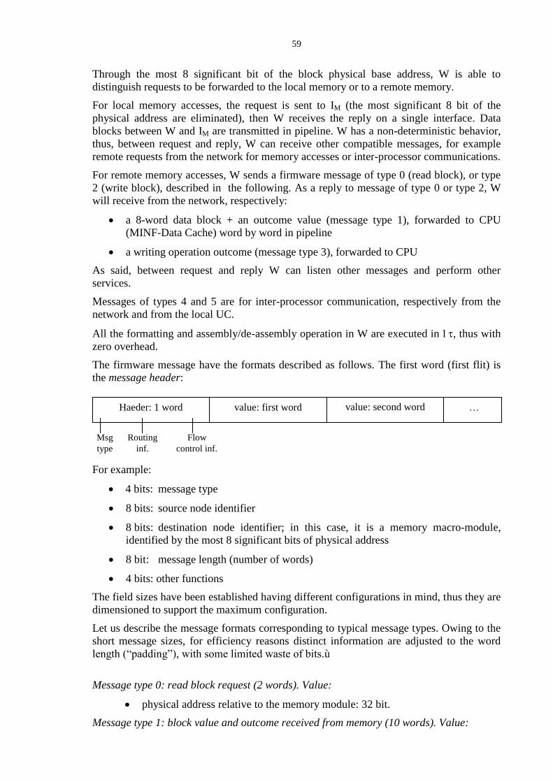
59
Through the most 8 significant bit of the block physical base address, W is able to
distinguish requests to be forwarded to the local memory or to a remote memory.
For local memory accesses, the request is sent to IM (the most significant 8 bit of the
physical address are eliminated), then W receives the reply on a single interface. Data
blocks between W and IM are transmitted in pipeline. W has a non-deterministic behavior,
thus, between request and reply, W can receive other compatible messages, for example
remote requests from the network for memory accesses or inter-processor communications.
For remote memory accesses, W sends a firmware message of type 0 (read block), or type
2 (write block), described in the following. As a reply to message of type 0 or type 2, W
will receive from the network, respectively:
a 8-word data block + an outcome value (message type 1), forwarded to CPU
(MINF-Data Cache) word by word in pipeline
a writing operation outcome (message type 3), forwarded to CPU
As said, between request and reply W can listen other messages and perform other
services.
Messages of types 4 and 5 are for inter-processor communication, respectively from the
network and from the local UC.
All the formatting and assembly/de-assembly operation in W are executed in , thus with
zero overhead.
The firmware message have the formats described as follows. The first word (first flit) is
the message header:
For example:
4 bits: message type
8 bits: source node identifier
8 bits: destination node identifier; in this case, it is a memory macro-module,
identified by the most 8 significant bits of physical address
8 bit: message length (number of words)
4 bits: other functions
The field sizes have been established having different configurations in mind, thus they are
dimensioned to support the maximum configuration.
Let us describe the message formats corresponding to typical message types. Owing to the
short message sizes, for efficiency reasons distinct information are adjusted to the word
length (“padding”), with some limited waste of bits.ù
Message type 0: read block request (2 words). Value:
physical address relative to the memory module: 32 bit.
Message type 1: block value and outcome received from memory (10 words). Value:
value: first word Haeder: 1 word value: second word
…
Msg
type
Flow
control inf.
Routing
inf.
60
outcome (8 bits);
not used (24 bits);
data (8 words).
Message type 2: write block request (10 words). Value:
block physical base address (32 bit);
data (8 words).
Message type 3: outcome of a block writing service from memory (2 words). Value:
outcome (8 bits);
not used (24 bits).
Message type 4: …
Message type 5: …
The figure in the following page illustrates the communications involved in a remote block
read operation. A path through the interconnection network crosses an average number of
switch nodes, given by dnet = 15 in the worst case, or dnet = 8 in the best case.
3.1.2 Memory access base latency
Referring to the figure, the remote memory access base latency for a cache block reading
operation is given by:
tao = TR-rem-0 = T0 + T1
where T0 and T1 are the latencies of the request phase and of the reply phase, respectively.
Let l be the length of a firmware message (according to the message type) and d the path
distance. We apply the general formula for the latency of structures with pipelined flow
control (Sect.2.5.4):
T0 = (2 l + d – 3) thop
Let the message of type 0, with l = 2, be originated by a data cache fault referred to a block
to be read from a remote memory macro-module. The path from the CPU to the remote
macro-module is MINF, Wsource, SW0, …, SWdnet-1, Wdest, IM-dest, all in pipeline, with
distance:
d = dnet + 4
Thus:
T0 = (5 + dnet ) thop
The reply message, of type 1, has length l = words.
The actions in remote M consist of a first sequential (i.e., not in pipeline) phase in which
the interleaved memory modules are read:
read request from IM to M: : thop,
modules are read in parallel: M,
words are transmitted in parallel from M to IM: thop.
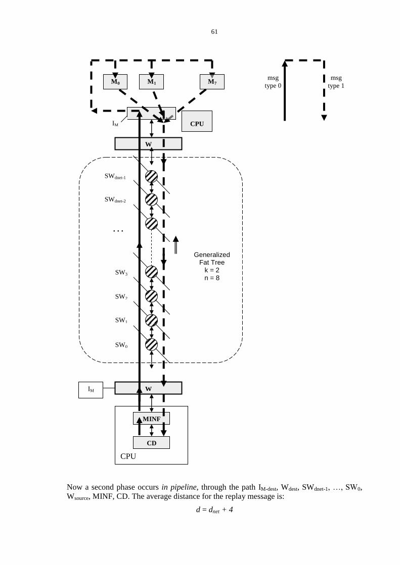
61
Now a second phase occurs in pipeline, through the path IM-dest, Wdest, SWdnet-1, …, SW0,
Wsource, MINF, CD. The average distance for the replay message is:
d = dnet + 4
msg
type 1
msg
type 0
CPU
. . . M0 M1
W
CPU
SWdnet-1
SWdnet-2
. . .
SW3
SW2
SW1
SW0
W
MINF
CD
Generalized
Fat Tree k = 2 n = 8
IM
IM
. . .
. . .
. . .
M7
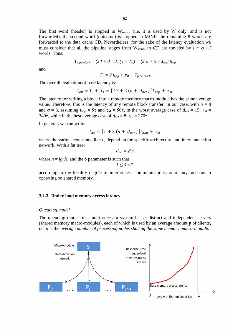
62
The first word (header) is stopped in Wsource (i.e. it is used by W only, and is not
forwarded), the second word (outcome) is stopped in MINF, the remaining 8 words are
forwarded to the data cache CD. Nevertheless, for the sake of the latency evaluation we
must consider that all the pipeline stages from Wsource to CD are traveled by l =
words. Thus:
Tpipe-block = (2 l + d – 3) ( + Ttr) = (2 + 5 +dnet) thop
and
T1 = 2 thop + M + Tpipe-block
The overall evaluation of base latency is:
𝑡𝑎0 = 𝑇0 + 𝑇1 = 12 + 2 𝜎 + 𝑑𝑛𝑒𝑡 𝑡𝑜𝑝 + 𝜏𝑀
The latency for writing a block into a remote memory macro-module has the same average
value. Therefore, this is the latency of any remote block transfer. In our case, with n = 8
and = 8, assuming thop = and M = , in the worst average case of dnet = 15: ta0 =
340, while in the best average case of dnet = 8: ta0 = 270.
In general, we can write:
𝑡𝑎0 = 𝑐 + 2 𝜎 + 𝑑𝑛𝑒𝑡 𝑡𝑜𝑝 + 𝜏𝑀
where the various constants, like c, depend on the specific architecture and interconnection
network. With a fat tree:
dnet = n
where n = lg2N, and the parameter is such that
1 ≤ < 2
according to the locality degree of interprocess communications, or of any mechanism
operating on shared memory.
3.1.3 Under-load memory access latency
Queueing model
The queueing model of a multiprocessor system has m distinct and independent servers
(shared memory macro-modules), each of which is used by an average amount p of clients,
i.e. p is the average number of processing nodes sharing the same memory macro-module.

63
Each server corresponds to a shared memory macro-module and to the interconnection
network paths from the p nodes to the shared macro-module itself, including the used
switch nodes:
In a SMP architecture, in which statistically the memory accesses are uniformly distributed
over the m macro-modules, p can be estimated as the mean of the binomial distribution
(Sect. 1.3.5):
𝑝 = 𝑁
𝑚
In a NUMA architecture, the uniform distribution does not hold, and the p value depends
on specific characteristics of the parallel program and its mapping onto the processing
nodes. In Sect. 3-1-4 we will discuss the mapping problem in NUMA architectures.
The under-load memory access latency is given by the server response time RQ.
In NUMA architectures it is meaningful to distinguish between remote memory access
latency (RQ-rem) and local memory access latency (RQ-loc). Assuming that, in case of conflict
between a remote request and a local request, this last is served with higher priority, we
can write:
RQ-loc = ta0-loc (1 + )
where is the server utilization factor, which is a result of the queueing model resolution.
Assumptions and approximations
The cost model for a shared memory multiprocessor implies a complex evaluation because
of the rather large number of variables, architectural variants and, perhaps most important,
many different situations that are related to the parallel application characteristics and to
the way in which the parallel computation exploits the multiprocessor architecture.
Our goal is to define a method for the under-load memory access evaluation, which is
characterized by an acceptable complexity and, at the same time, is able to capture the
essential elements of the problem. For this reason, we have to adapt an approximate
approach and to rely on some assumptions. The most meaningful assumptions are:
1. all the conflicts are concentrated on the memory macro-modules only, i.e. conflicts on
the network switch nodes and links have a negligible impact. Clearly, this assumption
is a simplification, which is reasonable for fat-tree based networks. For different kinds
of networks, in general also the conflicts along the interconnection network have to be
evaluated: the cost model could be improved to include such conflicts too;
2. let Tp be the mean time between two consecutive accesses of the same processing node
to a memory macro-module (during this time, the processor executes instructions
operating on registers, or primary cache). We assume that Tp be the mean value of an
exponentially distributed random variable. Actually this distribution depends on the
parallel application characteristics, and could be different from the exponential one.
However, for our purposes, we are interested in evaluating the interarrival time
distribution, which can be approximated as an exponential one because of the
independent behavior of the various processing nodes. In other words, for many
different distributions of the time between two consecutive accesses, the combination
of the requests of p processing nodes is approximately characterized by a random
behavior. Thus, for the WQ evaluation a good approximation is represented by the
M/D/1 queue. Again, a more accurate evaluation, taking into account the parallel
application characteristics, could be provided to improve the analysis;

64
3. the server service time is approximated as the base memory access latency. This means
that, if a request is blocked because of conflicts, it is blocked in the processing node.
Clearly, it is a worst-case assumption. In general, a request is blocked in an
intermediate switch node of the network, or in the macro-module interface. The best-
case assumption could be that the server service time is approximated as the memory
clock cycle. The most accurate evaluation lies in between, and it could be easily
provided to improve the analysis. We will adopt the worst-case assumption in order to
evaluate an upper bound of the under-load memory access latency.
Model resolution
Applying the methodology of Part1, Sect. 16, RQ is the solution of the system of equations:
1
),,(
0
0
p
TT
tT
T
T
tTWR
RTT
A
as
A
s
assQQ
Qp
From Sect. 16.1.2 of Part 1 we know that, for a M/D/1 queue:
)1(2)1(2
0
asQ tTW
The solution of the queueing model is a second degree equation in :
02 CBA
with coefficients:
000 2122 aapap tpCtpTBtTA
This equations has always two real, positive roots, 1 and 2, with 1 < 2, 1 < and 2 >
1. Thus, 1 is the solution of the queueing model.
According to this solution, the multiprocessor cost model will be studied in terms of RQ as
a function of the following parameters:
p: average number of processing nodes accessing the same memory macro-module,
Tp: mean time between two consecutive accesses to a memory macro-module,
N processing nodes, with n = lg2N network dimension,
: cache block size,
: relative network distance used in dnet = n,
thop = + Ttr : network hop latency,
M: memory clock cycle.

65
For each combination of such parameters, also the processing bandwidth and the relative
efficiency of the set of p clients will be evaluated. As discussed in Sect. 1.3.5, the
bandwidth value is a rough performance evaluation, measured as the average number of
instructions executed in the time unit. Thus, it is not a measure of the parallel program
performance, but just of the system ability to execute a certain amount of instructions in
presence of memory conflicts.
The true bandwidth and completion time of an application are evaluated according to the
cost model of the parallel program graph and of the used parallel paradigms. We know
that, in the application cost model, the physical architecture is abstracted through the Tsend
and Tcalc parameters:
Tsend is determined as a function of RQ, which is the queueing model solution,
Tcalc is determined as a function of Tp (calculation grain).
Some notable numeric evaluations are shown in the figures of the following pages, where
the cache block access latency is measured by RQ/, and the rough bandwidth is measured
in relative units.
The following observations are relevant:
1) The effect of p shows the importance of “low-p mappings” of parallel programs, as
it will be discussed in the next Section.
2) As it is expected, the effect of Tp is meaningful for fine grain computations (the
utilization factor increases), while for coarse grain computations the impact on
memory conflicts tends to become negligible, so the under-load latency tends to the
base one (ta0) for large Tp values.
3) The impact of N on the under-load latency is not so relevant, while it affects the
base latency. In terms of contention degradation, the relative parallelism degree is p
instead of N.
4) The impact of the cache block size is significant. However, if the macro-module
parallelism is high, larger blocks can be exploited: they have a positive impact on the
overall application bandwidth, since the number of remote accesses is proportionally
reduced. From this point of view, the importance of wormhole flow control has to be
remarked.
5) It is confirmed that the impact of is not too meaningful for low values of p. That
is, basically, for “low-p mappings” (see next Section), the communications tend to
be distance insensitive.
6) The impact of the memory clock cycle is significant for slow memory technologies.
However, notice that, owing to the memory hierarchy, the impact is limited for
memory clock cycles of the order of few tens .
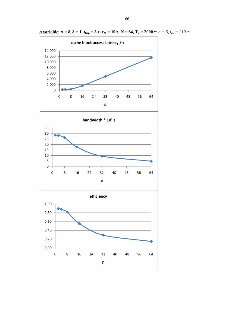
66
p variable; = 8, = 1, thop = 5 , M = 10 , N = 64, Tp = 2000 n = 6, ta0 = 210
0
2.000
4.000
6.000
8.000
10.000
12.000
14.000
0 8 16 24 32 40 48 56 64
p
tempo accesso blocco /
0
5
10
15
20
25
30
35
0 8 16 24 32 40 48 56 64
p
banda
0,00
0,20
0,40
0,60
0,80
1,00
0 8 16 24 32 40 48 56 64
p
efficienza
cache block access latency /
bandwidth * 103
efficiency
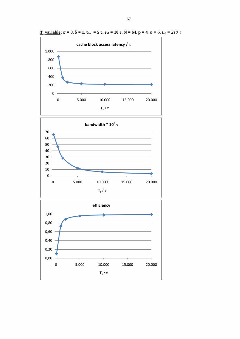
67
Tp variable; = 8, = 1, thop = 5 , M = 10 , N = 64, p = 4n = 6, ta0 = 210
0
200
400
600
800
1.000
0 5.000 10.000 15.000 20.000
Tp /
tempo accesso blocco /
0
10
20
30
40
50
60
70
0 5.000 10.000 15.000 20.000
Tp /
banda
0,00
0,20
0,40
0,60
0,80
1,00
0 5.000 10.000 15.000 20.000
Tp /
efficienza
cache block access latency /
bandwidth * 103
efficiency

68
p, Tp variables; = 8, = 1, thop = 5 , M = 10 , N = 64n = 6, ta0 = 210
0
2.000
4.000
6.000
8.000
10.000
12.000
14.000
0 8 16 24 32 40 48 56 64
p
tempo accesso blocco /
Tp=100
Tp=2.000
Tp=5.000
Tp=10.000
0
5
10
15
20
25
30
35
0 8 16 24 32 40 48 56 64
p
banda
Tp=100
Tp=2.000
Tp=5.000
Tp=10.000
0,00
0,20
0,40
0,60
0,80
1,00
0 8 16 24 32 40 48 56 64
p
efficienza
Tp=100
Tp=2.000
Tp=5.000
Tp=10.000
cache block access latency /
bandwidth * 103
efficiency
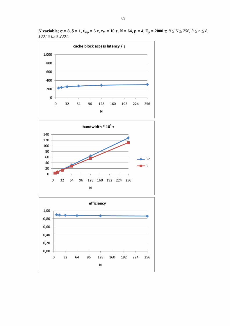
69
N variable; = 8, = 1, thop = 5 , M = 10 , N = 64, p = 4, Tp = 2000 8 ≤ N ≤ 256 3 ≤ n ≤ 8,
180 ≤ ta0 ≤ 230.
0
200
400
600
800
1.000
0 32 64 96 128 160 192 224 256
N
tempo accesso blocco /
0
20
40
60
80
100
120
140
0 32 64 96 128 160 192 224 256
N
banda
Bid
B
0,00
0,20
0,40
0,60
0,80
1,00
0 32 64 96 128 160 192 224 256
N
efficienza
cache block access latency /
bandwidth * 103 bandwidth * 103 bandwidth * 103 bandwidth * 103
efficiency
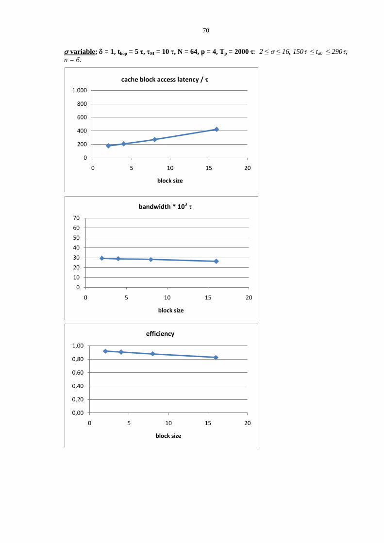
70
variable; = 1, thop = 5 , M = 10 , N = 64, p = 4, Tp = 2000 2 ≤ ≤ 16 150 ≤ ta0 ≤ 290; n = 6.
0
200
400
600
800
1.000
0 5 10 15 20
block size
tempo accesso blocco /
0
10
20
30
40
50
60
70
0 5 10 15 20
block size
banda
0,00
0,20
0,40
0,60
0,80
1,00
0 5 10 15 20
block size
efficienza
cache block access latency /
bandwidth * 103
efficiency
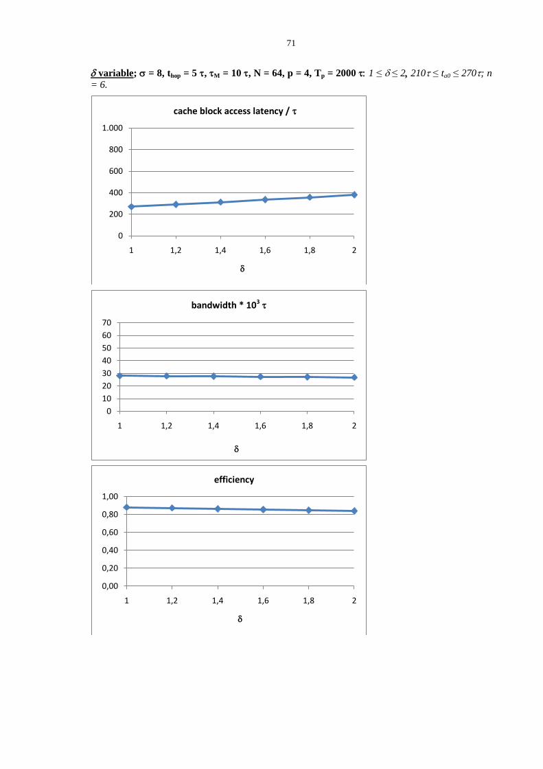
71
variable; = 8, thop = 5 , M = 10 , N = 64, p = 4, Tp = 2000 1 ≤ ≤ 2 210 ≤ ta0 ≤ 270; n
= 6.
0
200
400
600
800
1.000
1 1,2 1,4 1,6 1,8 2
tempo accesso blocco /
0
10
20
30
40
50
60
70
1 1,2 1,4 1,6 1,8 2
banda
0,00
0,20
0,40
0,60
0,80
1,00
1 1,2 1,4 1,6 1,8 2
efficienza
cache block access latency /
bandwidth * 103
efficiency
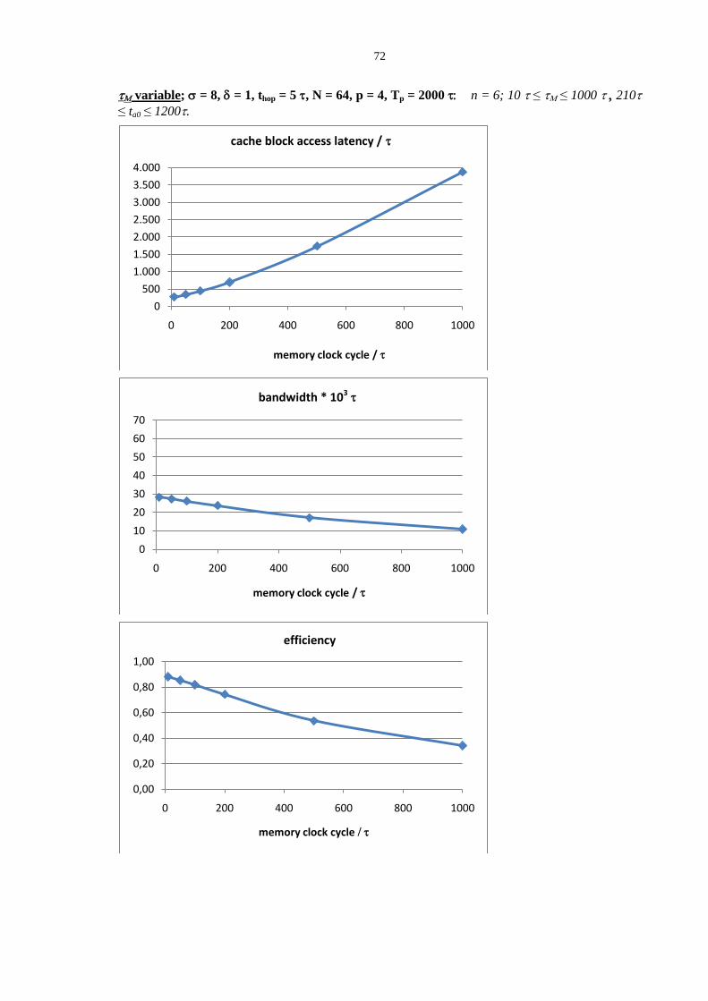
72
variable; = 8, = 1, thop = 5 , N = 64, p = 4, Tp = 2000 n = 6; 10 ≤ ≤ 1000 210
≤ ta0 ≤ 1200.
0
500
1.000
1.500
2.000
2.500
3.000
3.500
4.000
0 200 400 600 800 1000
memory clock cycle /
tempo accesso blocco /
0
10
20
30
40
50
60
70
0 200 400 600 800 1000
memory clock cycle /
banda
0,00
0,20
0,40
0,60
0,80
1,00
0 200 400 600 800 1000
memory clock cycle /
efficienza
cache block access latency /
bandwidth * 103
efficiency
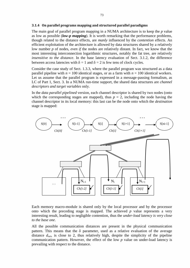
73
3.1.4 On parallel programs mapping and structured parallel paradigms
The main goal of parallel program mapping in a NUMA architecture is to keep the p value
as low as possible (low-p mapping). It is worth remarking that the performance problems,
though related to the distance effects, are manly influenced by the contention effects. An
efficient exploitation of the architecture is allowed by data structures shared by a relatively
low number p of nodes, even if the nodes are relatively distant. In fact, we know that the
most interesting interconnection logarithmic structures, notably the fat tree, are relatively
insensitive to the distance. In the base latency evaluation of Sect. 3.1.2, the difference
between access latencies with = 1 and = 2 is few tens of clock cycles.
Consider the case study of Sect. 1.3.3, where the parallel program was structured as a data
parallel pipeline with n = 100 identical stages, or as a farm with n = 100 identical workers.
Let us assume that the parallel program is expressed in a message-passing formalism, as
LC of Part 1, Sect. 3. In a NUMA run-time support, the shared data structures are channel
descriptors and target variables only.
In the data parallel pipelined version, each channel descriptor is shared by two nodes (onto
which the corresponding stages are mapped), thus p = 2, including the node having the
channel descriptor in its local memory: this last can be the node onto which the destination
stage is mapped:
Each memory macro-module is shared only by the local processor and by the processor
onto which the preceding stage is mapped. The achieved p value represents a very
interesting result, leading to negligible contention, thus the under-load latency is very close
to the base one.
All the possible communication distances are present in the physical communication
pattern. This means that the parameter, used as a relative evaluation of the average
distance dnet, is close to 2, thus relatively high, despite the simplicity of the pipeline
communication pattern. However, the effect of the low p value on under-load latency is
prevailing with respect to the distance.
Ch[0] Ch[i-1]
Ch[i]
Ch[i+1]
S[0]
. . . . . .
… Ni-1
Ni Ni+1
Ch[i-2]
Ch[i-1]
Ch[i]
S[i-1] S[i] S[i+1] S[ni-1]
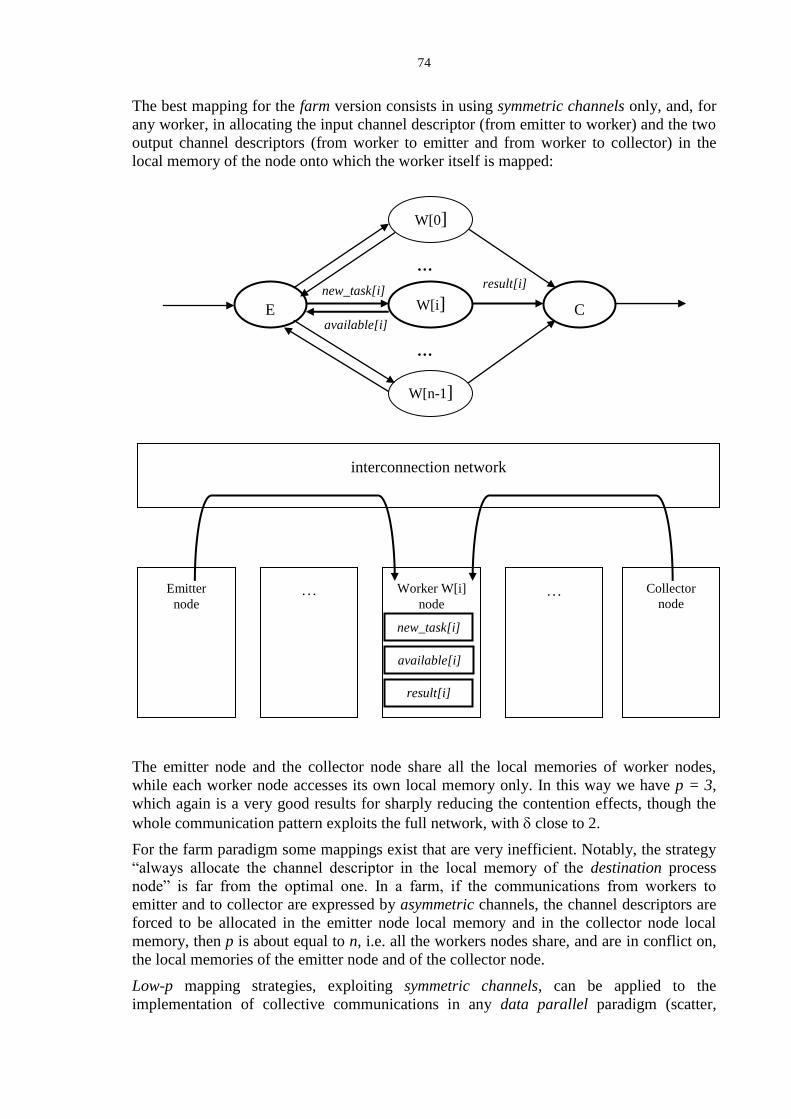
74
The best mapping for the farm version consists in using symmetric channels only, and, for
any worker, in allocating the input channel descriptor (from emitter to worker) and the two
output channel descriptors (from worker to emitter and from worker to collector) in the
local memory of the node onto which the worker itself is mapped:
The emitter node and the collector node share all the local memories of worker nodes,
while each worker node accesses its own local memory only. In this way we have p = 3,
which again is a very good results for sharply reducing the contention effects, though the
whole communication pattern exploits the full network, with close to 2.
For the farm paradigm some mappings exist that are very inefficient. Notably, the strategy
“always allocate the channel descriptor in the local memory of the destination process
node” is far from the optimal one. In a farm, if the communications from workers to
emitter and to collector are expressed by asymmetric channels, the channel descriptors are
forced to be allocated in the emitter node local memory and in the collector node local
memory, then p is about equal to n, i.e. all the workers nodes share, and are in conflict on,
the local memories of the emitter node and of the collector node.
Low-p mapping strategies, exploiting symmetric channels, can be applied to the
implementation of collective communications in any data parallel paradigm (scatter,
result[i]
available[i]
new_task[i]
…
…
E
W[0]
W[i]
W[n-1]
C
Emitter
node …
Collector
node
Worker W[i]
node …
new_task[i]
result[i]
available[i]
interconnection network

75
gather, multicast), as well as to collective operations (reduce), and to stencil
communications.
Also limited degree process structures are suitable for low-p mapping, notably
process trees
process rings and linear chains.
As a conclusion, we have verified another very important property of structured
parallelism paradigms: owing to the detailed knowledge of the process patterns, we are
able to identify some efficient implementation strategies, notably in terms of
communication forms and the related low-p mappings.
3.2 Inter-node communication latency in multicomputers
The multiprocessor evaluation could be extended to multicomputers too, at least from a
qualitative viewpoint.
In particular, since multicomputers are dedicated processors architectures,
the effect of low-p mappings is quite similar to what has been discussed about
NUMA multiprocessors.
Analogous considerations can be done about the impact of Tp and parameters:
coarse grain computations reduce the contention effects,
for low-p and coarse grain computations, logarithmic networks, like fat tree, are
basically distance insensitive.
However, quantitative evaluations are sensibly affected by the variable length of messages:
the approximations of the previous Section are less meaningful. Moreover, we wish to
consider both low dimension cubes and fat trees. For these reasons, in this Section the
analysis is completed with experimental and simulation studies: they are due to Fabrizio
Petrini.
It is worth remarking that some multicomputer architectures (MPP) exploit the firmware-
primitive network protocols, in the same way of multiprocessors, while others (simple
clusters) exploit IP-like protocols. In the latter case, the latency is largely dominated by the
IP protocol itself (notably, an overhead of about 105 instructions).
3.2.1 Performance measures for low dimension k-ary n-cubes
Assuming uniform traffic, the under-load latency has been estimated by Agarwal solving a
proper queueing model:
𝐿 = 1 + 𝜌 𝐵 (𝑘𝑑 − 1)
1 − 𝜌 𝑘𝑑2 (1 +
1
𝑛) 𝑛 𝑘𝑑 + 𝐵
where B is the packet size in flits (see wormhole flow control), and
𝑘𝑑 = 𝑘 − 1
2

76
is the average distance with unidirectional channels and toroidal connections. This model
is reported in the following figure, which respects the qualitative shape at the end of Sect.
2.2:
A meaningful result is that better latency is achieved with smaller packets: that is, small
packets utilize the network closer to its theoretical bandwidth, without significant
degradation in latency, and the average latency becomes less sensitive to congestion. This
result can be applied to shared memory multiprocessors too.
More robust models must take into account higher network loads or non-uniform traffic,
for example due to collective communications and other typical communication patterns of
parallel paradigms (Part 1).
The following figures have been derived by Fabrizio Petrini through simulation for a 16-
ary 2-cube under uniform traffic.

77
The first figure shows the bandwidth as a function of the packet size, the second the
comparison of deterministic vs adaptive routing strategies (the adaptive routing algorithm
is due to Duato):
Other simulation studies have been done for different traffic models.
3.2.2 Performance measures for Generalized Fat Trees
The following figures show some simulation results on Generalized Fat Trees. The
assumptions are:
1. uniform traffic,
2. minimal adaptive routing,
3. different number of logical communication channels inside the switch nodes,
4. Generalized Fat Tree based on a 4-ary 4-fly network.
78
The fourth assumption allows us to compare this network to the k-ary n-cube network
evaluated in Sect. 3.2.1, with the same number of processing nodes (N = 162 = 4
4 = 256). It
can be seen that, under the uniform traffic assumption, cube performances are better than,
or comparable to, fat trees.
However, it can be seen that, for more complex communication patterns, for example,
collective communications, the fate tree structures outperforms the cubes. This is due to the
fact that fat trees are much less sensitive to distance than cubes. For this reason, many
current commercial networks, including Myrinet and Infiniband, are basically structured as
fat trees.
A meaningful benchmark for complex communication patterns is represented by the so-
called complement traffic, in which
all nodes communicate simultaneously,
a node with binary identifier a0 a1 … an-1 sends messages to the node whose binary
identifier is 𝑎 0 𝑎1 … 𝑎𝑛−1 .
In other words, in a complement traffic pattern all the messages cross the network
bisection and traverse a path whose length is the network diameter. Thus, it is a latency-
sensitive pattern that stresses the network capability of dealing with a significant amount of
possible conflicts.
The following figure shows the relative bandwidths of
a) 16-ary 2-cube,
b) Generalized Fat Tree based on a 4-ary 4-fly network,
under complement traffic, using comparable technologies and minimal adaptive routing:
79
a)
b)
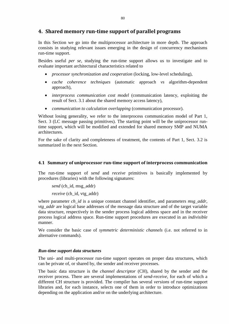
80
4. Shared memory run-time support of parallel programs
In this Section we go into the multiprocessor architecture in more depth. The approach
consists in studying relevant issues emerging in the design of concurrency mechanisms
run-time support.
Besides useful per se, studying the run-time support allows us to investigate and to
evaluate important architectural characteristics related to
processor synchronization and cooperation (locking, low-level scheduling),
cache coherence techniques (automatic approach vs algorithm-dependent
approach),
interprocess communication cost model (communication latency, exploiting the
result of Sect. 3.1 about the shared memory access latency),
communication to calculation overlapping (communication processor).
Without losing generality, we refer to the interprocess communication model of Part 1,
Sect. 3 (LC message passing primitives). The starting point will be the uniprocessor run-
time support, which will be modified and extended for shared memory SMP and NUMA
architectures.
For the sake of clarity and completeness of treatment, the contents of Part 1, Sect. 3.2 is
summarized in the next Section.
4.1 Summary of uniprocessor run-time support of interprocess communication
The run-time support of send and receive primitives is basically implemented by
procedures (libraries) with the following signatures:
send (ch_id, msg_addr)
receive (ch_id, vtg_addr)
where parameter ch_id is a unique constant channel identifier, and parameters msg_addr,
vtg_addr are logical base addresses of the message data structure and of the target variable
data structure, respectively in the sender process logical address space and in the receiver
process logical address space. Run-time support procedures are executed in an indivisible
manner.
We consider the basic case of symmetric deterministic channels (i.e. not referred to in
alternative commands).
Run-time support data structures
The uni- and multi-processor run-time support operates on proper data structures, which
can be private of, or shared by, the sender and receiver processes.
The basic data structure is the channel descriptor (CH), shared by the sender and the
receiver process. There are several implementations of send-receive, for each of which a
different CH structure is provided. The compiler has several versions of run-time support
libraries and, for each instance, selects one of them in order to introduce optimizations
depending on the application and/or on the underlying architecture.
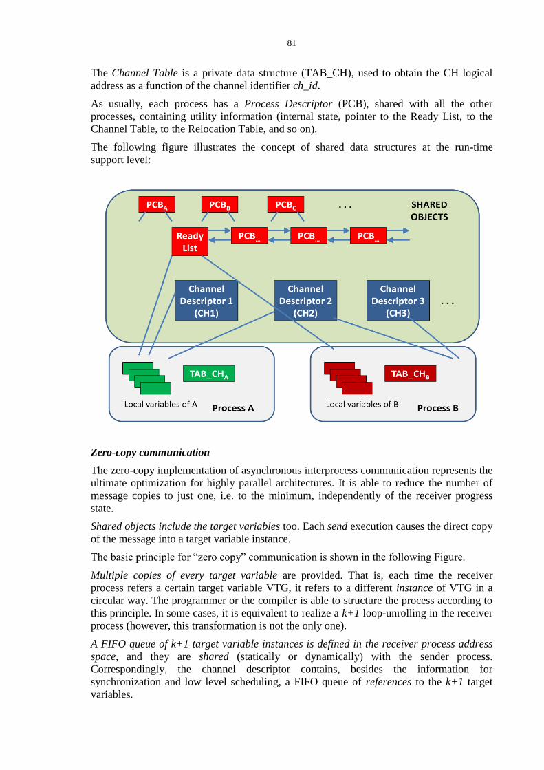
81
The Channel Table is a private data structure (TAB_CH), used to obtain the CH logical
address as a function of the channel identifier ch_id.
As usually, each process has a Process Descriptor (PCB), shared with all the other
processes, containing utility information (internal state, pointer to the Ready List, to the
Channel Table, to the Relocation Table, and so on).
The following figure illustrates the concept of shared data structures at the run-time
support level:
Zero-copy communication
The zero-copy implementation of asynchronous interprocess communication represents the
ultimate optimization for highly parallel architectures. It is able to reduce the number of
message copies to just one, i.e. to the minimum, independently of the receiver progress
state.
Shared objects include the target variables too. Each send execution causes the direct copy
of the message into a target variable instance.
The basic principle for “zero copy” communication is shown in the following Figure.
Multiple copies of every target variable are provided. That is, each time the receiver
process refers a certain target variable VTG, it refers to a different instance of VTG in a
circular way. The programmer or the compiler is able to structure the process according to
this principle. In some cases, it is equivalent to realize a k+1 loop-unrolling in the receiver
process (however, this transformation is not the only one).
A FIFO queue of k+1 target variable instances is defined in the receiver process address
space, and they are shared (statically or dynamically) with the sender process.
Correspondingly, the channel descriptor contains, besides the information for
synchronization and low level scheduling, a FIFO queue of references to the k+1 target
variables.
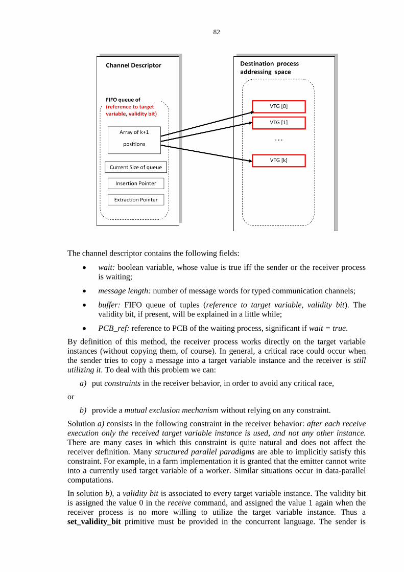
82
The channel descriptor contains the following fields:
wait: boolean variable, whose value is true iff the sender or the receiver process
is waiting;
message length: number of message words for typed communication channels;
buffer: FIFO queue of tuples (reference to target variable, validity bit). The
validity bit, if present, will be explained in a little while;
PCB_ref: reference to PCB of the waiting process, significant if wait = true.
By definition of this method, the receiver process works directly on the target variable
instances (without copying them, of course). In general, a critical race could occur when
the sender tries to copy a message into a target variable instance and the receiver is still
utilizing it. To deal with this problem we can:
a) put constraints in the receiver behavior, in order to avoid any critical race,
or
b) provide a mutual exclusion mechanism without relying on any constraint.
Solution a) consists in the following constraint in the receiver behavior: after each receive
execution only the received target variable instance is used, and not any other instance.
There are many cases in which this constraint is quite natural and does not affect the
receiver definition. Many structured parallel paradigms are able to implicitly satisfy this
constraint. For example, in a farm implementation it is granted that the emitter cannot write
into a currently used target variable of a worker. Similar situations occur in data-parallel
computations.
In solution b), a validity bit is associated to every target variable instance. The validity bit
is assigned the value 0 in the receive command, and assigned the value 1 again when the
receiver process is no more willing to utilize the target variable instance. Thus a
set_validity_bit primitive must be provided in the concurrent language. The sender is

83
suspended in the send execution if the validity bit of the target variable referred to by the
CH buffer is equal to 0.
Solution b) implies a context-switching overhead. It can be minimized by adopting some
proper strategies, notably increasing the asynchrony degree in order to reduce the
probability of finding the validity bit equal to zero;
The pseudo-code of zero-copy send run-time support for uniprocessor is shown in the
following figure, in the case of the validity bit utilization:
In the zero-copy cost model, the interprocess communication latency reduces to the send
latency only:
Lcom = Tsend = Tsetup + L Ttransm
Implementation in user space
Optimizations of send-receive run-time libraries, and zero-copy communication in
particular, must be designed according to a basic principle: they are executed in user space,
i.e. no privileged hierarchical states are exploited, in order to avoid the unnecessarily large
overhead of the transition into the supervisor state. For example, several additional
message copies are caused by the supervisor call mechanism.
In the HPC world, the most efficient, and/or most recent, run-time libraries of industrial
quality are implemented in user space.
Shared pointers
The necessity of shared references, used in the send-receive implementation (e.g. PCB
reference, target variable reference), requires a reasonable solution to indirectly referred
shared data structures, also called “shared pointers”.
84
Capability-based addressing (Part 1, Sect. 3.4.2) is a general and efficient solution based
on the dynamic allocation of objects in the logical address spaces, and is also characterized
by high protection degree.
4.2 Locking
Locking mechanisms are used to synchronize distinct processors executing sequences of
operations as indivisible, or atomic, actions. A sequence of operations, which can be
executed by more than one processor, is indivisible, or atomic, if no concurrent execution
is allowed for the sake of correctness. For example, let us consider two processors that can
execute the following computations:
Processor_1:: p; c; q
Processor_2:: r; c; s
Let us assume that the computation semantics is such that operation c must be executed at
most by one processor at the time (by Processor_1, or by Processor_2, but not both), while
no other constraint exists about the parallel execution of the various operations. This means
that c (which, in turn is a sequence of operations) is an atomic (sequence of) operation(s).
More in general, in
Processor_1:: p; c1; q
Processor_2:: r; c2; s
c1 and c2 are atomic if cannot be executed concurrently by Processor_1 and Processor_2.
Often (but not in general) atomic actions operate on modifiable shared data, that are
maintained in a consistent state if no concurrent manipulations is allowed, e.g. a read-
modify-write sequence.
Locking mechanisms extend what in a uniprocessor system is merely implemented through
interrupt disabling (in a multiprocessor this is just a necessary, but not sufficient, condition
for atomicity).
In the send run-time support (as in any other primitive at the process level), some
sequences to be rendered indivisible are:
a) read-modify-write sequences on the channel descriptor. For example:
< read the validity bit; if = 0:
read the buffer insertion pointer;
modify insertion pointer and buffer current size;
read the wait boolean; if true:
modify wait >
b) wake-up operations on the ready list in a SMP architecture.
In turn, a) sequence can be organized according to different schemes, in order to reduce its
duration, for example through a re-organization of the algorithm. A possible re-
organization consists in testing the wait boolean at the beginning of the sequence.
An indivisible sequence of actions is enclosed between two synchronization operations,
called lock and unlock, operating on a locking semaphore data type, for example:

85
lock (ch_semaphore);
read validity bit; if = 0:
read buffer insertion pointer;
modify insertion pointer and buffer current size;
read wait boolean; if true:
modify wait;
unlock (ch_semaphore);
This scheme implements a mutual exclusion of the enclosed sequence, i.e. at most one
processor at the time is able to execute this sequence. If several processors try to execute
the sequence simultaneously, then just one of them is able to complete the lock operation,
while the others are blocked inside the lock operation itself. Once the sequence is
completed, the unlock operation provides to unblock one of the possibly waiting
processors. This semantics is feasible provided that lock and unlock themselves are
indivisible operations.
Semantically, lock-unlock are similar to any semaphoric operation pair, like P-V or wait-
signal. However, the difference is that:
i) the lock-unlock atomicity is implemented directly at the firmware level (while the
P-V atomicity is implemented by lock-unlock brackets),
ii) the lock-unlock mechanism synchronizes processors (not processes), thus it implies
busy waiting (while P-V is characterized by the process transition into the waiting
state, accompanied by a context switch).
Point ii) implies an accurate trade-off between locking overhead minimization and
software lockout minimization, as discussed in Sect. 1.3.7.
4.2.1 Indivisible sequences o memory accesses
Point i) implies that
the lock-unlock atomicity is obtained recognizing, in the lock and unlock
algorithms, one or more indivisible sequences of memory accesses. For example, an
indivisible sequence of memory accesses could be: read (addr); read (addr + 1);
write (addr). In this example, only the memory accesses of an indivisible sequence
of operations are pointed out (e.g. it is possible that some calculation is done before
the write operation, but this is not of interest when the focus is on indivisible
sequences of memory accesses);
indivisible sequences of memory accesses are implemented with the help of the
shared memory arbitration mechanism. This can be done in at least two ways:
1. block the access to currently used locking semaphore locations,
or
2. block the access to the entire memory module containing the locking
semaphore.
In practice, because of the relatively short duration of lock and unlock sequences on
locking semaphores, the second solution is adopted.
86
INDIV bit and related processor mechanisms
This firmware mechanism, operating on the shared memory modules arbitration, employs
an additional bit, called indivisibility bit (indiv), belonging to the memory access request
generated by the processor, e.g.
memory access request = (logical address, data, memory operation,
memory hierarchy management annotations, indiv)
The indiv bit is forwarded towards the memory module (along with physical address, data,
and so on), and it is properly used by the one or more units in the interconnection path
from the processor to the memory module (as usually, in an all-cache architecture, this
situation occurs when a cache block is transferred from/into shared memory).
We can model an indivisible memory access sequence of h accesses in the following way:
all the first h-1 requests contain indiv = 1, and the h-th request contains indiv = 0.
Of course, in order that the indiv value is generated by the processor interpreter, the
assembler machine must contain proper instructions or annotations:
in many systems, assembler instructions for executing an indivisible read-modify-
write sequence on a single location exist. For example, Test and Set (R, Y),
Exchange (R, Y), Subtract from Memory (R,Y), Add to Memory (R, Y), where R
denotes a processor register and Y the address of the memory location on which the
sequence has to be performed;
a more powerful and flexible technique consists in annotations inserted in any
instruction that can refer shared memory locations (Load, Store).
In the didactic assembler machine D-RISC, both techniques are provided:
explicit SET_INDIV, RESET_INDIV and Exchange instructions,
set_indiv and reset_indiv annotations in Load and Store instructions.
Impact on memory behavior and interconnection structure
Once the assembler-level mechanisms are defined, the processor interpreter is
straightforward (merely, put the indiv bit to 1 or to 0 in the memory output interface). The
system strategy to implement indivisible sequences of memory accesses, according to the
indiv value, characterizes the specific multiprocessor architecture.
In order to understand the problem, consider initially the two extreme situations, in which
the interconnection structure is a crossbar or a single bus (Section 2.3):
a) in the crossbar-based architecture, a memory module (or its interface unit) has N
input distinct links, one from each processor. The memory module firmware
interpreter consists in non-deterministically testing all the N interfaces, in the same
clock cycle, and in selecting and serving one of the ready requests. Let J be the
interface identifier of the selected request. If this request contains indiv = 1, a
deterministic phase is entered: only the J-th interface is listened and served until a
request with indiv = 0 is received. During this period, all the other possible requests
are just waiting in their respective interfaces. When indiv = 0, the non-
deterministic behavior is resumed again. This mechanism is very efficient and
simple to implement, e.g. an explicit waiting queue is not necessary (it is
implemented by the unit interfaces themselves and by the non-deterministic
selection strategy);
87
b) in the bus-based architecture, a memory module (or its interface unit) has just one
input link from all the processors. The memory module firmware interpreter
consists in testing such interface and in serving the ready request. Let J be the
processor identifier associated to a received request. If this request contains indiv =
1, only the requests from the J-th processor are served until a request with indiv = 0
is received from processor J. All the other possible requests with processor
identifier different from J are received and explicitly buffered inside the unit. When
indiv = 0, the first queued request is served; if no queued requests exist, the input
interface is tested again. It should be noted that this explicit buffering (a FIFO
queue of N elements) is necessary, otherwise not even the requests from processor J
could be received and served (i.e., deadlock situation).
Consider now all the other limited degree interconnection networks studied in Sect. 2. The
scheme described in point a) cannot be adopted for any of them, i.e. in any architecture
based on a limited degree network (including the bus), an explicit buffering mechanism
must be provided.
For example, consider an SMP architecture with a k-ary n-fly network. The (unique) path
from a processor Pi to a memory module Mj is not exclusive of Pi, instead it contains some
sub-paths leading to Mj and shared by other processor subsets. From an indivisibility
modeling viewpoint, the set of Mj sub-paths is equivalent to a bus: it is impossible for the
memory module to listen only the processor which initiated the indivisible access
sequence; all the requests must the received, some of them are buffered and one is served.
In this kind of network, the queue could also be decentralized in the switch nodes
belonging to the path, however this decentralized solution does not offer any performance
advantage and complicates the switch design. Thus, a centralized buffer in each memory
unit is provided.
Quite similar considerations apply to the other limited degree networks. The reader is
invited to verify this concept for k-ary n-cubes and (fat) trees.
Memory congestion and fairness
Another important issue is related to the implementation of busy waiting in the execution
of a lock(x) operation. If a processor finds x = “red”, a loop of continuous read operations,
repeated until x = “green” is found, is not acceptable because:
the system congestion (shared memory module and interconnection network) is
unnecessarily increased,
the unlock execution itself is delayed by such attempts,
in presence of automatic cache coherence invalidation protocols, the cache block
containing the lock semaphore is invalided many times and unnecessarily. In fact,
in this case a sort of inefficient “ping-pong” effect occurs.
Two main classes of solutions exist:
a) periodic retry locking: the read attempts are spaced out by a constant time interval,
whose value is a function of the lock section duration (e.g. one half of such duration).
Theoretically, this solution is affected by the fairness problem, e.g. no processor is
guaranteed to enter a lock section in a finite time (though the probability of finding a
“red” semaphore is low);
b) fair locking: a fair solution is also able to minimize the contention effects. The lock
semaphore data structure contains a FIFO queue of processor names. If a processor

88
finds x = “red”, the processor name is inserted into the queue; the processor waits for
an unblocking interprocessor communication from the processor executing the
unlock operation. Just one access to the lock semaphore is needed for every lock
section, thus minimizing the system contention. This feature is especially valuable in
automatic cache coherence architectures with invalidation.
The efficiency, and the fairness, are paid with a slightly greater overhead because of
the queue manipulation (queue pointers and current size variables); however no
additional accesses to shared memory are done, provided that the semaphore data
structure (value, queue) is contained in the same cache block.
Finally, notice that, when lock sections are very short, e.g. just two memory accesses, lock-
unlock operations can be replaced by set_indiv and reset_indiv mechanisms themselves
directly. Though being an unfair solution, it is not affected by the congestion problem.
4.2.2 Lock – unlock implementations
Let us study the locking mechanism implementation according the above lines a) and b).
The pseudo-code notation
set indiv; S; reset indiv;
will be used for indivisible memory access sequences. They can be realized with explicit
instructions or with instruction annotations. For example, in D-RISC:
LOAD Rsemaphore, 0, Rtemp_semaphore, set_indiv
IF < test semaphore condition >
…
< manipulate the local semaphore value >
STORE Rsemaphore, 0, Rtemp_semaphore, reset_indiv
For each lock-unlock algorithm, an approximate evaluation of latency will be given.
Simply, the latency is evaluated as the number of shared memory accesses, i.e. cache block
transfer from / to the shared memory. The approximation consists in neglecting all the
local actions on registers or cache, which is quite acceptable.
1) Period retry locking
A simple boolean lock semaphore is used, initialed at the “true” value.
lock (semlock)::
ok = false;
while not ok do
set indiv;
if semlock then
semlock = false; reset indiv;
ok = true
else reset indiv;
busy waiting: execute a proper number of NOP
instructions
89
unlock (semlock)::
semlock = true
Lock latency (“green” semaphore): two shared memory access times.
Unlock latency: one shared memory access time.
2) Fair locking with FIFO queue
The lock semaphore is a struct (boolean value, FIFO queue of processor names).
Inizialization:: semlock.val = true; semlock.queue = empty.
lock (semlock)::
set indiv;
if semlock.val then
semlock.val = false; reset indiv
else
put (my_name, semlock.queue) ; reset indiv;
wait an I/O interrupt, generated by UC (Communication Unit) when an
unblocking interprocessor message is received
unlock (semlock)::
set indiv;
if empty (semlock.queue)
then
semlock.val = true; reset indiv
else
waiting_processor_name = get (semlock.queue); reset indiv;
send to UC an unblocking interprocessor message, with destination =
waiting_processor_name
Lock latency: two shared memory access times for any value of the semaphore (of course, the “red”
semaphore situation implies busy waiting)
Unlock latency: one plus one shared memory access times. Notice that the lock semaphore words
are stored in distinct modules of an interleaved macro-module. However, it is sufficient to execute
set_indiv on the first module only (where semlock.val is stored): this requires an additional access
in the unlock operation (e.g. an “empty” read).
It should be remarked that locking per se is a low-latency mechanism, provided that primitive
elementary supports exist at the assembler and firmware level. This is not the situation when the
available locking mechanisms are operating system calls to be executed in kernel space. However,
implementing the run-time support on top of an operating system is inefficient both for the
excessive overhead (see the discussion about the minimization of copies, Part 1, Sect. 3.4.1), and
for the much higher impact of software lockout (high values of parameter L).
In the following, we assume that synchronization in the run-time support design is realized by
locking mechanisms executed in user space, implemented by the primitive firmware and assembler
mechanisms described above, and that short lock sections are designed.

90
4.2.3 Locked version of interprocess communication run-time support
The uniprocessor version of run-time support is the basis for the multiprocessor version.
The main modifications concern the low-level scheduling (see subsequent Sections) and
the synchronization of critical sections. For this last aspect, it is sufficient that the critical
sections are enclosed in lock-unlock brackets.
The channel descriptor is modified with the addition of a lock semaphore:
X: lock semaphore;
Wait: boolean;
Message_length: integer;
Buffer: FIFO queue of (k + 1) positions (reference to target variable, validity bit)
PCB_ref: reference to PCB
The X semaphore is used for the mutual exclusion of all the critical sections
(“communication sections”), except the ones used in low-level scheduling actions.
Communications sections are the same for SMP and for NUMA multiprocessors.
The straightforward modification to the zero-copy send run-time support, with respect to Sect. 4.1,
is the following:
send (ch_id, msg_address) ::
CH address =TAB_CH (ch_id);
lock (X);
if (CH_Buffer [Insertion_Pointer].validity_bit = 0) then
wait = true;
copy reference to Sender_PCB into CH.PCB_ref ;
unlock (X);
process transition into WAIT state: context switching ;
copy message value into the target variable referred by
CH_Buffer [Insertion_Pointer].reference_to_target_variable ;
modify CH_Buffer. Insertion_Pointer and CH_Buffer_Current_Size;
if wait then
wait = false;
wake_up partner process (CH.PCB_ref) ;
if buffer_full then
wait = true;
copy reference to Sender_PCB into CH.PCB_ref ;
unlock (X);
process transition into WAIT state: context switching
else unlock (X)
91
This version can be optimized in order to reduce the size of lock sections, because of the software
lockout problem.
A first optimization is the following:
send (ch_id, msg_address) ::
CH address =TAB_CH (ch_id);
lock (X);
if (CH_Buffer [Insertion_Pointer].validity_bit = 0) then
wait = true;
copy reference to Sender_PCB into CH.PCB_ref ;
unlock (X);
process transition into WAIT state: context switching ;
if wait then
unlock (X);
copy message value into the target variable referred by
CH_Buffer [Insertion_Pointer].reference_to_target_variable ;
modify CH_Buffer. Insertion_Pointer and CH_Buffer_Current_Size;
case wait, buffer_full of
false, false: unlock (X);
false, true: wait = true;
copy reference to Sender_PCB into CH.PCB_ref ;
unlock (X);
process transition into WAIT state: context switching
true, : wait = false;
wake_up partner process (CH.PCB_ref) ;
The code executed when the validity bit is zero has a very low probability, thus it has negligible
impact on the L parameter.
The most important optimization is: the communication critical section is of “zero length” if the
partner is waiting.
Moreover, another important optimization could be introduced: the message copy could be
executed outside the critical section, also when the partner is not in waiting state.
This optimization is left as an exercise.
92
4.3 Low-level scheduling
As said, the low-level scheduling, and in particular the process wake-up phase, is specific
of each architecture.
4.3.1 Preemptive wake-up in anonymous processors architectures
In an anonymous processors (SMP) architecture, the non-preemptive wake-up procedure
consists merely in inserting the PCB of the waked-up process into the unique shared Ready
List, operating in lock state. A lock semaphore is associated to the Ready List.
If a priority-based preemptive scheduling is provided, the following strategy is realized in
order to exploit the anonymity feature:
let B be a waiting process;
let A be a process, running on processor Pi, which executes a primitive waking up
process B;
let C be a process, running on processor Pj, which has the minimum priority among
all the N running processes;
if priority (B) priority (C), then A executes the non-preemptive wake-up
procedure, putting PCBB into the Ready List, and the wake-up procedure ends;
otherwise, if priority (B) > priority (C), then a preemption action occurs in
processor Pj: C passes into the ready state and B passes directly into the running
state. This is done according to one of the two following alternatives:
o if i = j, thus A C, and the preemption action is executed by A itself on Pi,
and the wake-up procedure ends;
o otherwise, if i ≠ j, then A sends an interprocessor message to Pj in order to
cause the execution of the preemptive action on such processor. The
preemption message contains the reference to PCBB. As usually, the
received interprocessor message is transformed by UCj into an interrupt,
which is handled by the running process C: the interrupt handler procedure
consists just in the preemption action.
The information about the minimum priority running process must be available to A. For
this purpose, a shared Central Table is provided. It contains N entries, each one
corresponding to a distinct processor and containing the priority of the currently running
process and other utility information. This Table can be implemented as an ordered list,
and is updated at every context switch.
It is possible that a certain inconsistency occurs in the above procedure: during the
interprocessor communication, processor Pj could have executed a context switch, or
modified the C priority, so that the priority of the Pj running process is no longer less than
the B priority value. Notice that such an inconsistency does not imply an incorrect
behavior, but just a temporary lack of scheduling optimization. Processor Pj can
execute the context switch, without worrying about the lack of optimization,
or
execute the whole preemptive wake-up procedure again, as if it were the waking-up
process A. In theory, this can cause a “bouncing” procedure, which is not

93
guaranteed to terminate in a finite time. In practice, after a very limited number of
“bounces”, the context switch is executed in any case. This solution requires that
the interprocessor message includes also the B priority value.
The task of verifying the consistency of interprocessor request, and possibly of accessing
the Central Table and starting the “bouncing” procedure, can be delegated to a “smart”
UCj, thus avoiding to interrupt CPUj unnecessarily.
4.3.2 Process wake-up in dedicated processors architectures
In a dedicated processor architecture, the low-level scheduling operations on a process
allocated on Pj can be executed only by one of the Pj processes. If a process A, running on
Pi, wishes to wake-up a process B, allocated on Pj:
if i = j, then a local wake-up procedure is executed by A, exactly as in a
uniprocessor system (with or without preemption);
otherwise, if i ≠ j, A sends an interprocessor message to Pj in order to cause the
execution of the local wake-up procedure on such processor. The wake-up message
contains the reference to PCBB. As usually, the received interprocessor message is
transformed by UCj into an interrupt, which is handled by the running process C:
the interrupt handler procedure consists just in the wake-up procedure.
4.4 Run-time support and cache coherence
In Sect. 1.3.5, we have discussed general problems related to cache coherence in parallel
applications, both in a shared-objects model and in a message-passing model,
distinguishing between the management of shared objects belonging to the run-time
support only and shared objects under the responsibility of the application programmer.
Now we go into the cache coherence issues in more depth with regard to the cache
coherence impact on the interprocess communication run-time support design. Therefore,
the shared data structures to be kept cache-coherent are the run-time support ones, in
particular the channel descriptors (and associated locking semaphores, target variable, and
similar) in a message-passing model and, for SMP architectures, the ready list.
We will study, and compare, the implementation according to the automatic invalidation
cache coherence approach and to the algorithm-dependent one (Sect. 1.3.5).
In this analysis, a central role is played by the presence of processor synchronization
through locking mechanisms. For this reason, we focus on the analysis and evaluation of a
lock section: it can be (a part of) the code of the run-time support executed in lock state.
We distinguish between two cases:
a) one-to-one synchronization: a lock semaphore synchronizes two processors, for
example in the run-time support of a LC send-receive communication on a
symmetric channel:
Pi:: Pj::
lock (X); lock (X);
CS1; CS2;
unlock (X); unlock (X);
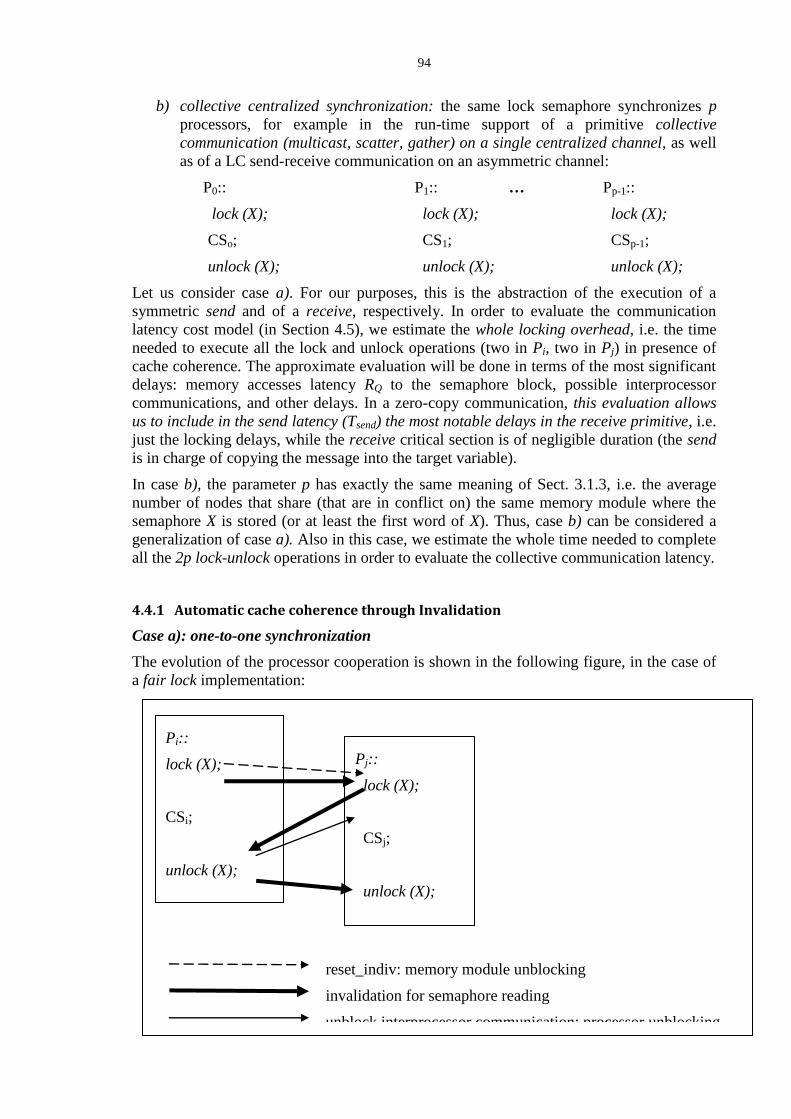
94
b) collective centralized synchronization: the same lock semaphore synchronizes p
processors, for example in the run-time support of a primitive collective
communication (multicast, scatter, gather) on a single centralized channel, as well
as of a LC send-receive communication on an asymmetric channel:
P0:: P1:: … Pp-1::
lock (X); lock (X); lock (X);
CSo; CS1; CSp-1;
unlock (X); unlock (X); unlock (X);
Let us consider case a). For our purposes, this is the abstraction of the execution of a
symmetric send and of a receive, respectively. In order to evaluate the communication
latency cost model (in Section 4.5), we estimate the whole locking overhead, i.e. the time
needed to execute all the lock and unlock operations (two in Pi, two in Pj) in presence of
cache coherence. The approximate evaluation will be done in terms of the most significant
delays: memory accesses latency RQ to the semaphore block, possible interprocessor
communications, and other delays. In a zero-copy communication, this evaluation allows
us to include in the send latency (Tsend) the most notable delays in the receive primitive, i.e.
just the locking delays, while the receive critical section is of negligible duration (the send
is in charge of copying the message into the target variable).
In case b), the parameter p has exactly the same meaning of Sect. 3.1.3, i.e. the average
number of nodes that share (that are in conflict on) the same memory module where the
semaphore X is stored (or at least the first word of X). Thus, case b) can be considered a
generalization of case a). Also in this case, we estimate the whole time needed to complete
all the 2p lock-unlock operations in order to evaluate the collective communication latency.
4.4.1 Automatic cache coherence through Invalidation
Case a): one-to-one synchronization
The evolution of the processor cooperation is shown in the following figure, in the case of
a fair lock implementation:
Pi::
lock (X);
CSi;
unlock (X);
Pj::
lock (X);
CSj;
unlock (X);
reset_indiv: memory module unblocking
invalidation for semaphore reading
unblock interprocessor communication: processor unblocking

95
Without losing generality, we assume that Pi (with cache Ci) and Pj (with cache Cj) try the
lock (X) execution simultaneously, and that Pi is able to read the X block. That is, the read
request of Pj is blocked (queued) by the indivisibility bit mechanism.
Pi executes lock (X) and enters the critical section.
The reset indiv, at the end of lock (X), unblocks Pj, which now is able to read the X block
by invalidating the X block in Ci. On the other hand, Pi does no more need such block. Pj
has acquired the lock semaphore, however it is blocked in the lock (X). According to the
lock implementation, Pj is
periodically testing the local value of X in Cj, until Pi will invalidate, and acquire, X
in order to modify it in the unlock. The next attempt of Pj to read X will cause the
invalidation, then X will be modified locally in Cj,
or
waiting for an unblock interprocessor communication (from Pi).
At the end of the critical section, Pi executes the unlock(X): the read request operation
causes the invalidation of the X block in Cj (on the other hand, Pj is not really using X) and
the X block acquisition in Ci. At the end of the unlock, Pj is unblocked by Pi
implicitly (periodic retry lock): in this case the X block is read into Cj by
invalidating the X block in Ci (on the other hand, it is no more used by Pi) – this
situation is not shown in the Figure,
or
explicitly (fair lock): X is not read – this is the situation shown in the Figure.
Finally, the unlock(X) execution in Pj
with fair locking: causes the invalidation of X block in Ci (where it is no more used)
and its acquisition in Cj,
with periodic retry locking: finds the lock semaphore already in Cj.
This description is useful to highlight a significant aspect: in presence of processor
synchronization: the automatic cache coherence strategy per se does not imply inefficient
“ping-pong” effects. When a processor invalidates a block, the other processor is blocked
or is not using the block itself.
The invalidation mechanism has a cost. We assume that an invalidation is implemented by
one write operation of the old owner into the shared main memory, followed by a read
operation of the new owner. Thus, its cost is equivalent to two remote memory accesses,
i.e. 2RQ. Even if the implementation does not really consist in the two memory accesses
described above (e.g. copying from Ci into Cj), the final effect is equivalent in terms of
latency. This evaluation is valid for both multiprocessor organizations, SMP or NUMA,
and for both writing techniques, Write-Back or Write-Through.
Notice that such evaluation is a rather optimistic one, because we are not taking into
account the invalidation mechanism overhead for the snoopy bus control or the directory
manipulation: we are just evaluating the invalidation cost in terms of memory block
transfers.
Because we are evaluating the whole effect of lock-unlock in both processors, 8 accesses
are required to complete the computation in Pi and Pj, both for the retry and the fair
locking. Therefore:
one-to-one synchronization latency 8 RQ

96
The processor unblocking interprocessor communication in the fair solution occurs in
parallel to the computation of Pi and Pj, thus its cost can be neglected as a first
approximation.
Notice that the lock-unlock operations do not exploit reuse, thus the automatic cache
coherence does not introduce advantages compared to architectures in with the lock
semaphores are not cacheable.
It is important to notice that, if explicit locking mechanisms are not employed, the cache
coherence mechanism itself could be used for synchronization purposes too, provided that
explicit lock-free and cache coherence based algorithms are designed: this is not without
consequences on programmability. That is, the promise of the cache coherence invisibility
is not kept: without locking the designer must deal with the cache coherence issues
explicitly. In terms of performance, the software lockout avoidance might be paid with an
additional overhead of the cache coherence mechanism and some “ping-pong”
occurrences.
Case b): collective centralized synchronization
This case is illustrated in the following figure:
As shown, it is a generalization of one-to-one synchronization to one-to-p or p-to-one
centralized synchronizations. Two linear chains of invalidations are driven by the lock
synchronization mechanism. In the figure, it is exemplified the case of two chains ordered
from P0 to Pp-1, assuming that P0 is the first processor able to enter the critical section.
However, any ordering is feasible for two p-step chains.
Thus by evaluating the interprocessor communication latency as RQ:
collective centralized synchronization latency 4 p RQ
P0::
lock (X);
CS0;
unlock (X);
P1::
lock (X);
CS1;
unlock (X);
reset_indiv: memory module unblocking
invalidation for semaphore reading
unblock interprocessor communication: processor unblocking
P2::
lock (X);
CS2;
unlock (X)
P3::
lock (X);
CS3;
unlock (X);

97
which coincides with the one-to-one evaluation when p = 2.
It is confirmed the importance of low-p mappings of parallel programs, as discussed in
Sect. 3.1.4.
4.4.2 Algorithm-dependent cache coherence
In this approach, a less or equal number of shared memory accesses is done, without the
additional overhead of the automatic management, and some further improvements can be
achieved.
Some assembler-level annotations, or directives, for cache management are useful, or
necessary, in this approach. In D-RISC they are called:
STORE …, deallocate explicit block de-allocation
STORE …, not_deallocate explicit block permanence in cache
STORE …, re_write_block explicit block copy into shared memory
STORE …, write_through single word writing in shared memory
Case a): one-to-one synchronization
Let us assume that Pi executes lock (X) which is concluded with an explicit block re-
writing into the shared memory.
The reset indiv, at the end of lock (X), unblocks Pj, which now is able to read the X block;
however it is blocked in the lock (X). According to the lock implementation, Pj is
periodically retrying the X block acquisition, or waiting for an unblock interprocessor
communication (from Pi).
If the period retry locking is adopted, Pi does not deallocate X from Ci, while deallocation
is necessary with the fair locking technique.
At the end of the critical section, Pi executes the unlock(X): X is already in Ci with the
period retry locking, while X must be read again with the fair locking technique.
At the end of the unlock(X), Pj is unblocked by Pi, implicitly or explicitly (fair lock: X is
not read).
We can see that no additional overhead is introduced in the algorithm-dependent
approach, since just “normal” memory-cache transfers are performed without any other
mechanism.
Thus:
one-to-one synchronization latency = 6 RQ or 8 RQ
respectively for the periodic retry or the fair locking techniques, since in the periodic retry
solution the block X has not been deallocated at the end of the lock operation.
Moreover, some significant improvements can be achieved. Notably, the memory access
latency for the re-writing operations can be reduced by modifying just one word, instead of
an entire block, as allowed by the annotation write-through. Notice that this cannot be
implemented in an automatic cache coherence strategy.
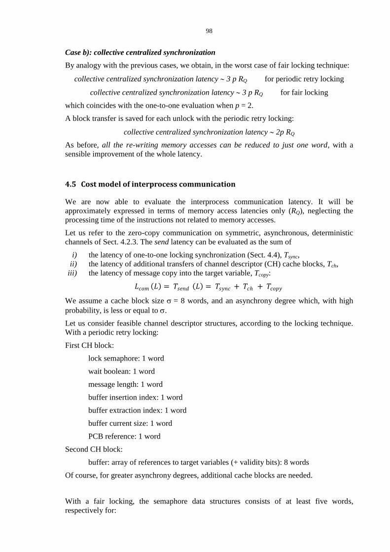
98
Case b): collective centralized synchronization
By analogy with the previous cases, we obtain, in the worst case of fair locking technique:
collective centralized synchronization latency 3 p RQ for periodic retry locking
collective centralized synchronization latency 3 p RQ for fair locking
which coincides with the one-to-one evaluation when p = 2.
A block transfer is saved for each unlock with the periodic retry locking:
collective centralized synchronization latency 2p RQ
As before, all the re-writing memory accesses can be reduced to just one word, with a
sensible improvement of the whole latency.
4.5 Cost model of interprocess communication
We are now able to evaluate the interprocess communication latency. It will be
approximately expressed in terms of memory access latencies only (RQ), neglecting the
processing time of the instructions not related to memory accesses.
Let us refer to the zero-copy communication on symmetric, asynchronous, deterministic
channels of Sect. 4.2.3. The send latency can be evaluated as the sum of
i) the latency of one-to-one locking synchronization (Sect. 4.4), Tsync,
ii) the latency of additional transfers of channel descriptor (CH) cache blocks, Tch,
iii) the latency of message copy into the target variable, Tcopy:
𝐿𝑐𝑜𝑚 𝐿 = 𝑇𝑠𝑒𝑛𝑑 𝐿 = 𝑇𝑠𝑦𝑛𝑐 + 𝑇𝑐 + 𝑇𝑐𝑜𝑝𝑦
We assume a cache block size = 8 words, and an asynchrony degree which, with high
probability, is less or equal to .
Let us consider feasible channel descriptor structures, according to the locking technique.
With a periodic retry locking:
First CH block:
lock semaphore: 1 word
wait boolean: 1 word
message length: 1 word
buffer insertion index: 1 word
buffer extraction index: 1 word
buffer current size: 1 word
PCB reference: 1 word
Second CH block:
buffer: array of references to target variables (+ validity bits): 8 words
Of course, for greater asynchrony degrees, additional cache blocks are needed.
With a fair locking, the semaphore data structures consists of at least five words,
respectively for:
99
semaphore value: 1 word
processor queue insertion index: 1 word
processor queue extraction index: 1 word
processor queue current size: 1 word
processor queue: at least 1 word
To save space, the processor queue can be implemented in the following way: few words
contain the names of the first queued processors in FIFO order. If more processors are
queued (a rare event), their names are encoded by a bit mask, where each bit position
correspond to a processor name. This requires few additional words.
Thus, the first cache block is needed for the lock semaphore only, and, in the most
probable situation, the channel descriptor has two further blocks.
In conclusion,
periodic retry locking: the cache transfer latency Tsync is exploited also for the
manipulation of those channel descriptor information which are stored in the same
semaphore block. Thus, since the second block is not modified by the send
primitive:
Tch = 2 RQ
taking into account also the latency on the receive side.
fair locking: Tsync is exploited for the lock synchronization only. Thus:
Tch = 4 RQ
The message copy consists in a loop of message block reading operationss (from the local
memory in a NUMA machine) and writing operations into shared remote memory. A
pipeline implementation is able to hide the message block reading latency; it can be
realized through the block prefetching option, or by a proper realization of the node
interface unit (W). Thus, Tcopy reduces to the writing latency only:
𝑇𝑐𝑜𝑝𝑦 𝐿 = 𝐿
𝜎 𝑅𝑄
𝐿𝑐𝑜𝑚 𝐿 = 𝑇𝑠𝑒𝑛𝑑 𝐿 = 8 𝑅𝑄 + 𝐿
𝜎 𝑅𝑄
Thus (for L multiple of :
𝑇𝑠𝑒𝑡𝑢𝑝 = 8 𝑅𝑄 𝑇𝑡𝑟𝑎𝑛𝑠𝑚 = 𝑅𝑄
𝜎
With fair locking:
𝐿𝑐𝑜𝑚 𝐿 = 𝑇𝑠𝑒𝑛𝑑 𝐿 = 12 𝑅𝑄 + 𝐿
𝜎 𝑅𝑄
Thus (for L multiple of :
𝑇𝑠𝑒𝑡𝑢𝑝 = 12 𝑅𝑄 𝑇𝑡𝑟𝑎𝑛𝑠𝑚 = 𝑅𝑄
𝜎
The Tsetup formula can be rendered a bit more accurate by considering the probability of
executing low-level scheduling actions. On the other hand, we have not taken into account
the possible improvements due to the single word re-writing option.

100
Using the results of Sect. 3.1.4 about the under-load memory access latency, with values of
RQ of the order of 102 - 10
3 clock cycles, we have the typical values of the communication
cost model parameters:
𝑇𝑠𝑒𝑡𝑢𝑝 = 𝑎 103 𝜏 𝑇𝑡𝑟𝑎𝑛𝑠𝑚 = 𝑏 102 𝜏
with a and b constants ranging in the intervals (0,5 - 20) and (0,1 - 2) respectively.
4.6 Communication processor
We know that, in some parallel program patterns, the interprocess communication latency
might be overlapped to the calculation time.
The needed architectural support consists in a communication processor (KP) associated to
the main processor (IP) of the processing node. KP is dedicated, or specialized, to the
execution of the run-time support functionalities, and in particular the send primitive. The
principle is the following:
when IP has to execute a send primitive on an asynchronous channel, it delegates
this task to KP and continues the execution;
the receive primitive is executed by IP entirely.
The architectural scheme of the processing node is based on a shared memory cooperation
between IP and KP. This can be achieved by realizing the node as a small multiprocessor
with dedicated processors, for example:
where MI and MK are local memories (or secondary caches, if the node is integrated on a
single chip) of IP and KP respectively.
Equivalently, KP may be an input-output coprocessor, sharing memory with IP through
DMA and Memory mapped I/O. In particular, this kind of implementation is adopted when
the communication processor is provided “inside” the interconnection network box. That
is, the externally available links of the interconnection network (i.e. the links to be
connected to the processing nodes) are I/O links.
IP
MI
KP
MK
Interconnection Network
uc uc
W-IP W-KP
W-node Processing node
101
The parameter passing from IP to KP is done by reference (by capability) through shared
memory, without additional copies. IP prepares a data structure S containing the channel
identifier and the message reference. The reference to S is transmitted to KP via I/O (in the
Figure; via the pair of communication units uc-uc). KP is a “daemon”, that, once activated
by the interrupt from IP, acquires the parameters into its addressing space, with very low
overhead, and starts the send execution.
In this example, we have a clear proof of the capability role in the “shared pointer
problem” (Part 1, Sect. 3.4.2). The KP process must share any possible messages, target
variables and PCBs of communicating processes. A static allocation of such objects in the
KP addressing space is extremely inefficient or practically impossible. The dynamic
allocation allowed by the capability addressing solves the problem in an elegant and
efficient manner.
Though it is possible to realize KP with the same architecture of IP, the trend is to design a
much simpler CPU-KP, possibly specialized at the firmware level, as discussed in the
multicore solutions of Sect. 1.5.4.
Let us know analyze the send implementation in more depth.
The send semantics is: copy the message and, if the asynchrony degree becomes saturated
(buffer_full), suspend the sender process. Of course, this condition must by verified in
presence of KP too.
If IP delegates the send execution entirely to KP, then some complications are introduced
in the send implementation because of the management of the waiting state of the sender
process, and if we wish to achieve the objective of delegating more than one asynchronous
communications (on the same channel or on different channels) overlapped to the same
calculation section, e.g.
calculation …; send …; send …; send …; …
A simpler and efficient solution, able to achieve this objective, consists in the following
principle:
IP itself verifies the saturation of channel asynchrony;
IP delegates to KP the send continuation;
if (buffer_size = k) IP sets the wait boolean variable in the channel descriptor, and
suspends the sender process (if k denotes the asynchrony degree, k + 1 is the
number of buffer elements);
In the zero-copy communication, IP controls the validity bit too, if provided.
The channel descriptor is locked by IP and unlocked by KP.
This scheme eliminates the complexity of the general solution (full delegation to KP), at
the expense of an initial phase executed by IP itself, thus not overlapped to the internal
calculation. In the interprocess communication cost model, the latency of this phase must
be included in the Tcalc parameter. In practice, the overlapping is applied to the channel
descriptor buffer manipulation, to the message copy, and to the low-level scheduling
actions on the destination process.
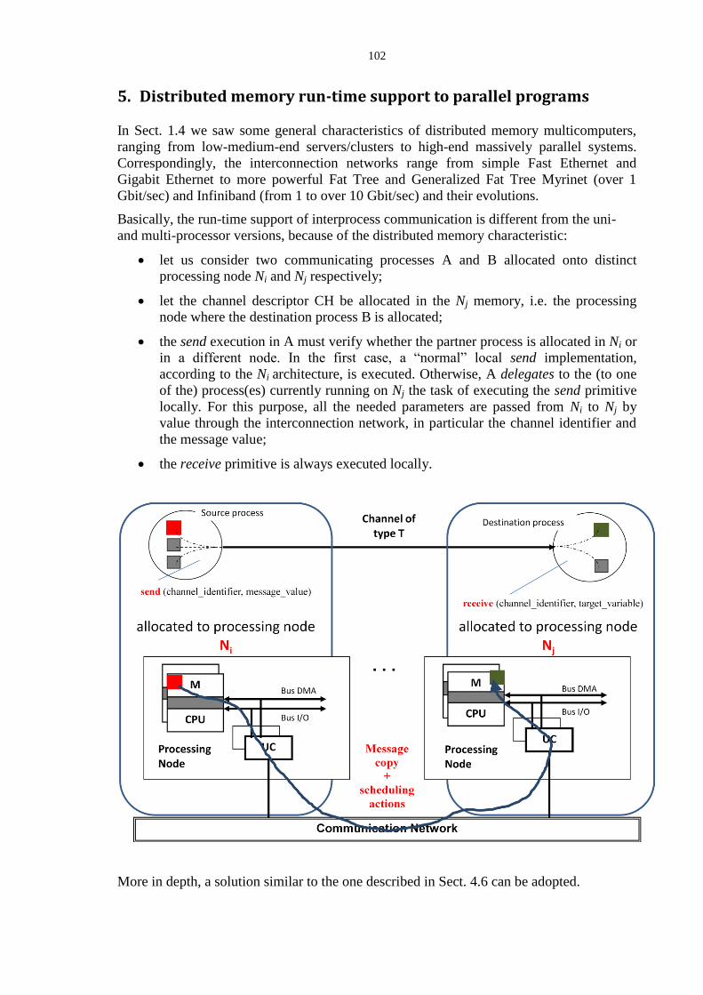
102
5. Distributed memory run-time support to parallel programs
In Sect. 1.4 we saw some general characteristics of distributed memory multicomputers,
ranging from low-medium-end servers/clusters to high-end massively parallel systems.
Correspondingly, the interconnection networks range from simple Fast Ethernet and
Gigabit Ethernet to more powerful Fat Tree and Generalized Fat Tree Myrinet (over 1
Gbit/sec) and Infiniband (from 1 to over 10 Gbit/sec) and their evolutions.
Basically, the run-time support of interprocess communication is different from the uni-
and multi-processor versions, because of the distributed memory characteristic:
let us consider two communicating processes A and B allocated onto distinct
processing node Ni and Nj respectively;
let the channel descriptor CH be allocated in the Nj memory, i.e. the processing
node where the destination process B is allocated;
the send execution in A must verify whether the partner process is allocated in Ni or
in a different node. In the first case, a “normal” local send implementation,
according to the Ni architecture, is executed. Otherwise, A delegates to the (to one
of the) process(es) currently running on Nj the task of executing the send primitive
locally. For this purpose, all the needed parameters are passed from Ni to Nj by
value through the interconnection network, in particular the channel identifier and
the message value;
the receive primitive is always executed locally.
More in depth, a solution similar to the one described in Sect. 4.6 can be adopted.

103
A partial view of the channel descriptor (CHs) is available in Ni. It contains the following
main information:
processing node in which the destination process is allocated,
message length,
asynchrony degree,
wait boolean variable,
number of the currently buffered messages.
For a remote communication, an information packet (source node, destination node,
message length, channel identifier, message value source process identifier) is sent to the
Communication Unit (UC) in DMA, and from UC over the network to the destination
node.
The sender process verifies the asynchrony degree saturation in CHs and, if buffer_full,
passes into the waiting state.
It is a task of the receive primitive to cause the updating of the number of buffered
messages in CHs, via an interprocessor message from Nj to Ni. In Ni, the interrupt handler
updates the number of currently buffered messages in CHs and checks the wait boolean: if
true, the source process is waked-up.
The following Figures summarize the distributed run-time support implementation.

104
About the interprocess communication cost model, also according to the study of Sect. 3.2,
we can say that:
If the communication network is used with the primitive firmware routing and
flow-control protocol, we achieve similar results to the shared memory run-time:

105
o for systems realized in a rack
Tsetup , Ttransm
o otherwise, for long distance networks, the transmission latency dominates,
e.g.
Tsetup , Ttransm
till
If the communication network is used with the IP protocol, i.e., the application is
IP-dependent, an additional overhead is paid due to the protocol actions (e.g.,
formatting, de-formatting) inside the nodes (plus transmission overhead on long
distance networks):
o on rack: Tsetup , Ttransm
o on long distances: Tsetup , Ttransm

106
6. Questions and exercises
1) Assume that a wormhole Generalized Fat Tree network, with ariety k = 2 and n = 8, is
used in a SMP architecture with a double role: a) processor-to-memory interconnection,
and b) processor-to-processor interconnection. The firmware messages contain in the first
word: routing information (source identifier, destination identifier), message type (a or b),
and message length in words. Links and flits size is one word.
Describe the detailed (e.g., at the clock cycle grain) behavior of a switching node.
2) Consider a k-ary 2-cube interconnection network with deterministic routing and
wormhole flow control (one-word links, one-word flits).
Describe the structure and behavior of a Network Node. The description should clearly
show whether it is feasible to achieve the maximum bidirectional bandwidth, provided that
the proper traffic conditions hold.
3) Implement in detail the lock operation according to the fair algorithm. Evaluate its
latency in case of green semaphore.
4) Find an alternative implementation of zero-copy send primitive, able to reduce the
locking critical section duration.
5) Consider the preemptive wake-up procedure in a SMP architecture. In order to avoid the
consistency problem arising in the processor to be preempted, a complex locking
procedure could be implemented: which data structures should have been locked, and
when unlocked ?
That is, implement the preemptive wake-up procedure in such a way that the situation
detected by the waking process doesn’t change until the wake-up has been completed.
6) Consider a NUMA multiprocessor architecture with 128 nodes. Each node includes a D-
RISC pipelined CPU without secondary cache. Data cache blocks are 4-word wide. Local
memory locations are 128-bit wide. The maximum capacity of main memory is 512 Giga
words. The interconnection structure is of logarithmic kind, with one-word links and
wormhole flow control. All the system processing units have the same clock cycle ,
except the local memory units having a clock cycle equal to . Any inter-chip link has a
transmission latency.
a) Explain the architecture of a generic node. Show the structure of firmware
messages used for local memory accesses and for remote memory accesses, and
explain how and where they are built.
b) Determine the base latency of local memory accesses and of remote memory
accesses.
c) Explain the qualitative impact of parameter p (the average number of nodes
accessing the same memory module) on the memory access latency. Estimate a
reliable value of p for a system executing a parallel program structured as a 16-
stage pipeline, where each stage is a 4-worker farm.

107
d) Evaluate the interprocess communication latency approximately, in terms of the
base memory access latencies only, assuming zero-copy communication and 4-
word messages. Referring to the example in point c), estimate the approximation
degree of this evaluation compared to the evaluation in terms of under-load
memory access latencies.
7) Let’s assume that the source code of run-time support for send and receive
communication primitives is available in a uniprocessor version for a given assembler-
firmware architecture S. We try to exploit this code for other kinds of architecture at best.
Explain which parts can be preserved, and which parts have to be modified/replaced and in
which way, for a) SMP, b) NUMA, and c) cluster architectures, exploiting the given
uniprocessor architecture S as building block. Explain possible specific features required to
S for the a), b), c) implementations.
8)
a) Consider the under-load memory access latency in all-cache multiprocessor
architectures. For all the parameters, that have influence on such latency, discuss their
qualitative impact. Where possible, introduce some quantitative considerations, in
particular under which conditions the impact of each parameters is more or less
significant.
b) Consider an all-cache NUMA architecture with 32 nodes connected by a toroidal ring
with wormhole flow control and 32-bit links. Show the architecture of a generic node
based on D-RISC pipelined CPU. Evaluate the base memory access latency. Explain
qualitatively, yet formally, why the under-load memory access latency decreases by
replacing the single ring with m independent toroidal rings.
9) Consider the architectures with communication processor. Assuming KP identical to IP,
a multiprocessor with N processing nodes has a total of 2N CPUs. Thus the problem arises:
why not exploiting 2N processing nodes without communication processors?
Discuss this problem, individuating pros and cons of the communication processor
solution.
10) Study algorithm-dependent solutions to cache coherence applied to the secondary
caches in SMP architectures.
11) Describe the send and receive run-time support in detail for a multicomputer
architecture.
12) Consider a multicomputer in which the nodes have an internal multiprocessor
architecture.
Study the implications on the interprocess communication run-time support, distinguishing
between SMP and NUMA architectures.
108
13) General scheme of exercises integrating Part 1 and Part 2:
Consider the parallel programming exercises of Part 1, for example Sect. 17, 18.
Study their implementations on a SMP architecture and on a NUMA architecture. In
particular, discuss
a) how the memory hierarchy is exploited,
b) how the shared data structures are mapped.
Assume typical reasonable values for the parameters characterizing the memory hierarchy,
and suitable logarithmic interconnection networks for the SMP and for the NUMA
architecture.
Moreover:
c) assuming that the given values of Tsetup and Ttransm have been estimated for a certain
value of p, discuss under which conditions such estimate is accurate for the given
computation and its mapping (all the other parameters of the cost model are
assumed to be verified).