Embed Size (px)
Citation preview

ParMooN – a modernized program package based onmapped finite elements
Ulrich Wilbrandta, Clemens Bartscha, Naveed Ahmeda, Najib Aliaa,1, FelixAnkera,2, Laura Blanka, Alfonso Caiazzoa, Sashikumaar Ganesanb,3, Swetlana
Gierea, Gunar Matthiesc, Raviteja Meesalab, Abdus Shamimb, JagannathVenkatesanb, Volker Johna,d,4,∗
aWeierstrass Institute for Applied Analysis and Stochastics, Leibniz Institute inForschungsverbund Berlin e. V. (WIAS), Mohrenstr. 39, 10117 Berlin, GermanybDepartment of Computational and Data Sciences, Indian Institute of Science,
Bangalore - 560012, Indiac Department of Mathematics, Institute of Numerical Mathematics, TU Dresden,
01062 Dresden GermanydFree University of Berlin, Department of Mathematics and Computer Science, Arnimallee
6, 14195 Berlin, Germany
Abstract
ParMooN is a program package for the numerical solution of elliptic andparabolic partial differential equations. It inherits the distinct features of itspredecessor MooNMD [28]: strict decoupling of geometry and finite elementspaces, implementation of mapped finite elements as their definition can befound in textbooks, and a geometric multigrid preconditioner with the optionto use different finite element spaces on different levels of the multigrid hierar-chy. After having presented some thoughts about in-house research codes, thispaper focuses on aspects of the parallelization for a distributed memory environ-
∗Corresponding author.Email addresses: [email protected] (Ulrich Wilbrandt),
[email protected] (Clemens Bartsch), [email protected](Naveed Ahmed), [email protected] (Najib Alia), [email protected](Felix Anker), [email protected] (Laura Blank),[email protected] (Alfonso Caiazzo), [email protected] (SashikumaarGanesan), [email protected] (Swetlana Giere),[email protected] (Gunar Matthies), [email protected] (RavitejaMeesala), [email protected] (Abdus Shamim), [email protected](Jagannath Venkatesan), [email protected] (Volker John)
1The work of Najib Alia has been supported by a funding from the European Union’sHorizon 2020 research and innovation programme under the Marie Sk lodowska-Curie grantagreement No. 675715 (MIMESIS).
2The work of Felix Anker has been supported by grant Jo329/10-2 within the DFG priorityprogramme 1679: Dynamic simulation of interconnected solids processes.
3The work of Sashikumaar Ganesan has partially been supported by the Naval ResearchBoard, DRDO, India through the grant NRB/4003/PG/368.
4The work of Volker John has partially been supported by grant Jo329/10-2 within theDFG priority programme 1679: Dynamic simulation of interconnected solids processes.
Preprint submitted to Elsevier December 23, 2016

ment, which is the main novelty of ParMooN. Numerical studies, performedon compute servers, assess the efficiency of the parallelized geometric multigridpreconditioner in comparison with some parallel solvers that are available inthe library PETSc. The results of these studies give a first indication whetherthe cumbersome implementation of the parallelized geometric multigrid methodwas worthwhile or not.
Keywords: Mapped finite elements; Geometric multigrid method;Parallelization;
1. Introduction
MooNMD, a C++ program package for the numerical solution of ellipticand parabolic partial differential equations based on mapped finite elements, isdescribed in [28]. A modernized version of this package, called ParMooN, hasrecently been developed to be used as a research code in the future.
The core of MooNMD was designed more than 15 years ago and this codehas been successfully used in many scientific studies. There are almost 90 re-search articles citing MooNMD via [28], see [37]. Recent advances in computinghardware and language standards necessitate a re-design and re-implementationof some of the core routines. With the new core and the new features, the codewas renamed to ParMooN (Parallel Mathematics and object-oriented Numer-ics).
The general aims of this paper are to report on the development of the exist-ing research code towards the new package ParMooN in order to accomplishthe desired features of an in-house research code that will be formulated inSection 2 and to assess the parallelized geometric multigrid method by compar-ing it with solvers that are available in an external library. The original codepossesses some distinct features that should be transferred to ParMooN, likethe strict decoupling of geometry and finite element spaces, the implementationof mapped finite elements as their definition can be found in textbooks, and amultiple discretization multilevel (MDML) preconditioner. This paper focuseson the most relevant aspect concerning the development of ParMooN, namelythe distributed memory parallelization. In particular, the technically most cum-bersome part, the parallelization of the geometric multigrid, is discussed.
A main contribution of this paper is a first assessment of the resulting par-allel geometric multigrid method in comparison with parallel solvers for linearsystems of equations that can be called from the library PETSc. The numericalstudies were performed on compute servers as the available in-house hardware.We think that this assessment is also of interest for other groups who developtheir own codes in order to get an impression whether it is worthwhile to im-plement a parallelized geometric multigrid method or not. Two main problemclasses supported in ParMooN are considered in the numerical studies: scalarconvection-diffusion-reaction equations and the incompressible Navier–Stokesequations.
2

The paper is organized as follows. Section 2 contains an exposition of ourthoughts about in-house research codes, in particular about their advantages andtheir goals. Mapped finite elements, as they are used in MooNMD/ParMooN,are described in Section 3. Section 4 presents main aspects of the parallelizationand the parallelization of the geometric multigrid method is briefly discussed inSection 5. Numerical studies that compare this method with solvers availablein PETSc are presented in Section 6. The paper concludes with a summary.
2. Some Considerations about In-House Research Codes
Nowadays, several academic software packages for solving partial differentialequations exist in the research community. They are usually developed andsupported by research groups for whom software development is one of themain scientific tasks. Such software packages include, among others, deal.II[10], FEniCS [2], DUNE [15, 11], OpenFOAM [32], or FreeFem++ [19].These packages have advanced functionality and support features like adaptivemesh refinement, parallelism, etc.
Naturally, a research code developed in-house possesses less functionalitythan these large packages. In view of their availability, the following questionsarise: Why is it worth to develop an own research code? In particular, isit worth to develop a code within a research group that focuses primarily onnumerical analysis? In the following, some arguments, mainly based on our ownexperience, are presented.
In-depth knowledge of details of the software. The first key aspect of workingwith a code developed and maintained within the research group is the detailedknowledge of the software structure. In fact, applied mathematicians oftenwork at the development of numerical methods. These methods have to beimplemented, assessed, and compared with popular state-of-the-art methods forthe same problem. A meaningful assessment requires the usage of the methodsin the same code. In this respect, it is important to have access to a code whereone knows and can control every detail.
For brevity, just one example will be mentioned to show the importance ofknowing the details of a software package. This example concerns the clar-ification of appropriate interface conditions in subdomain iterations for theStokes–Darcy problem, see [13]. Standard Neumann interface conditions canbe used only for viscosity and permeability coefficients that are unrealisticallylarge. For realistic coefficients, appropriate Robin boundary conditions have tobe used. The implementation of the Robin interface conditions was performedin a straightforward way in MooNMD/ParMooN.
Flexibility. Further advantages of an own research code are the possibility ofcontrolling its core parts and flexibility. In particular, for our research it is veryimportant that the code supports the use of different discretization strategies.As an example, MooNMD was designed for finite element methods. But forthe investigation of discretizations of time-dependent convection-diffusion equa-tions in [29], finite difference methods were implemented as well. Because these
3

methods performed very well, they were later used in the context of simulatingpopulation balance systems defined in tensor-product domains, e.g., see [36].
Testing of numerical methods. MooNMD was used in the definition ofbenchmark problems in [23]. The list of examples could be extended. In addi-tion, a number of numerical methods have been developed and implemented inour research code which turned out to be not (yet) competitive, like the opti-mization of stabilization parameters in SUPG methods in [27]. Having a knownand flexible research code at disposal allows to test and support methods that,at the time of the implementation, have not been benchmarked in detail.
Certainly, also the large packages mentioned above allow the implementa-tion of different methods and discretization strategies. However, we think thata successful implementation often requires a very close interaction with coredevelopers of the packages. This effort might not be feasible for both the userand the developer. Therefore, an own code might reduce the time from thedevelopment to the assessment of numerical methods.
Benefits for students. A further aspect, related to the interaction of the coredevelopment team, concerns the students and the PhD students who are involvedin the development and in the usage of the code. Since the core developers ofan own research code are readily available and they are experts in the focusedresearch topics of the group, these students can be supported efficiently. Inaddition, students working at the code stated several positive effects: the workat details of the implementation facilitates the insight into the methods andalgorithms, which is important for analyzing their properties, and it enhancesthe skills in software design and management.
Of course, incorporating students into code development requires that thereis an easy use of the code and an easy access to basic routines, such as, in thecase of a finite element solver, assembling of matrices and solving linear systemsof equations. This issue touches already the next question: What should beexpected from an own research code?
Easy usage. In order to support students starting to work with the code, aneasy installation and basic testing setup are essential. There are even successfulattempts for designing complex codes that can be used for teaching studentsin basic courses on numerical methods for partial differential equations, likethe so-called computational laboratory for Investigating Incompressible FlowProblems (IFISS), see [16], which uses Matlab, and the open source softwareFreeFem++ [19], which is based on an own language.
Modularity. The code should be modular. In particular, there should be ageneral core and individual projects are attached to this core. Of course, theprojects use routines from the core. But using an own code, it seems to be easierthan with a large package, which is developed somewhere else, to incorporatecontributions from the projects into the core.
Stability. With respect to the required stability of the code, there are, inour opinion, no fundamental differences between own research codes and largepackages.
Efficiency. However, there are different expectations with respect to theefficiency. A research code should be flexible in many respects, since its main
4
tasks include supporting the development of numerical methods and resultsfrom numerical analysis. For instance, in the code MooNMD/ParMooN, theconcept of mapped finite elements is implemented, see Section 3. In this way,the code supports currently around 170 finite elements in two dimensions and 75finite elements in three dimensions. Consequently, all routines are implementedfor the general situation. For certain finite elements, this might be less efficientthan using tailored routines. However, also for a research code, efficiency is a keyproperty that should not be neglected. For instance, the simulation of standardacademic benchmark problems for turbulent incompressible flows requires thecomputation of large time intervals to collect temporal averages of statistics ofinterest. In our opinion, an own research code should be reasonably efficienton the available in-house hardware, which, in our case, are usually laptops,compute servers, or small clusters.
3. Mapped Finite Element Spaces
The implementation of finite element methods in MooNMD/ParMooNis based on a rather abstract definition of a finite element space and on themapping of each mesh cell to a reference cell.
Let Ω ⊂ Rd, d ∈ 2, 3, be a bounded domain and let T h be an admissibletriangulation of Ω consisting of compact, simply connected mesh cells. Foreach mesh cell K, a local finite element space P (K) ⊂ Cs(K), s ≥ 0, is givenby some finite-dimensional space of functions spanned by a basis φK,iNK
i=1.
Furthermore, a set of local linear functionals ΦK,iNKi=1 is given. The space
P (K) is unisolvent with respect to the functionals. Often, a so-called localbasis is chosen, i.e., a basis that satisfies ΦK,i(φK,j) = δij for i, j = 1, . . . , NK .The local linear functionals might be values of the functions or their derivativesin certain points, integrals on K or on faces of K.
Let Φ1, . . . ,ΦN : Cs(Ω) → R be given continuous linear functionals. Therestriction of each functional to Cs(K) defines the set of local functionals. Theunion of all mesh cells Kj , for which there is a p ∈ P (Kj) with Φi(p) 6= 0, willbe denoted by ωi. Now, the global finite element space is defined as follows. Afunction v(x) defined on Ω with v|K ∈ P (K) for all K ∈ T h is called continuouswith respect to the functional Φi if Φi(v|K1
) = Φi(v|K2) for all K1,K2 ∈ ωi.
The space
S =v ∈ L∞(Ω) : v|K ∈ P (K) and v is continuous with respect to
Φi, i = 1, . . . , N
is called finite element space. The global basis φjNj=1 of S is defined by theconditions φj ∈ S with Φi(φj) = δij for i, j = 1, . . . , N .
Using this definition for the implementation of a finite element space requires1.) the definition of the local basis and linear functionals for each K,2.) the implementation of a method that assures continuity with respect to
the functionals stated in the definition of S.
5

The first requirement can be achieved in two different ways, via a mappedor an unmapped implementation. In the unmapped approach, the local basisand linear functionals are defined directly on K. In contrast, mapped finiteelements are closely connected to a standard way of analyzing finite elementdiscretizations. This analysis consists of three steps:• Map an arbitrary mesh cell K to a compact reference mesh cell K.• Prove the desired properties on K, which is the core of the analysis.• Map the reference mesh cell K back to K to get the final result.
Hence, this approach has two main features:• All considerations have to be done on K only.• Information about neighbor mesh cells ofK is neither available nor needed.
Mapped and unmapped finite element methods possess the same analyticalproperties if the reference map FK : K → K is affine for every mesh cell K ofthe given triangulation, e.g., compare [14, Chap. 2.3]. In the case of non-affinemaps, occurring, e.g., for a triangulation consisting of arbitrary quadrilateral orhexahedral mesh cells, mapped and unmapped finite element spaces might bedifferent. In MooNMD/ ParMooN, the concept of mapped finite elements isimplemented in the following way. Reference mesh cells are the unit simplices,e.g., in two dimensions with the vertices (0, 0), (1, 0), (0, 1), and the unit cubesK = [−1, 1]d. Affine maps are available for all reference mesh cells. To accountfor arbitrary quadrilaterals and hexahedra, d-linear maps are also implementedfor the unit cubes. Based on the different reference cells, local spaces on K,linear functionals, and reference maps, MooNMD/ParMooN currently sup-ports about 170 finite elements in two dimensions and 75 finite elements in threedimensions.
The use of mapped finite element spaces essentially requires the implementa-tion of finite elements on the reference cells. The quadrature rules for numericalintegration have to be implemented only on these cells, since the integrals onphysical cells are transformed to integrals on the reference cells. Note that thesame strategy works also for the handling of cell faces, which are mapped ontolower-dimensional reference cells by corresponding reference maps.
Concerning requirement 2.) above, a finite element space S is representedby a map F called d.o.f.-manager which maps local, i. e., within a cell, indicesof degrees of freedom (d.o.f.) to global ones. For this purpose define M(K) tobe the set of local d.o.f.s denoted by (K, i) on the cell K. Then define the setof all local degrees of freedom
M :=⋃
K∈T h
M(K).
The local-to-global map F now surjectively maps M to 1, . . . , N such thatF((K, i)) = F((K ′, j)) whenever the local degrees of freedom (K, i) and (K ′, j)belong to the same global degree of freedom. The number N ≤ |M | is then thenumber of global degrees of freedom. In other words, F describes a partition Pof the set M (i. e., an equivalence relation) together with a global numbering.Computing such a map F is done via Algorithm 1 in ParMooN.
6

Algorithm 1: Computation of F that maps local degrees of freedom to global ones. The inputis a mesh T h whose cells K are ordered by increasing integers id(K).
1 P ← finest partition of M
2 for all mesh cells K ∈ T h
3 determine M(K)4 for all neighbors K′ of K with id(K) < id(K′)5 determine M(K′)6 find local partition Ploc of M(K) ∪M(K′)7 P ← finest partition coarser than P and Ploc
8 assign increasing integers to each subset in the partition P
A B
C D
1 2
3 4
1 2
3 4
1 2
3 4
1 2
3 4
F
A B
C D
1 2
3 4
2 5
4 6
3 4
7 8
4 6
8 9
Figure 1: A 2× 2 mesh with Q1 finite elements. Left: Local degrees of freedom in each cell.Right: Global degrees of freedom after the application of algorithm 1.
Initially the partition is set to be the finest partition of the set M , i. e., itconsists of disjoint single-element subsets, so that no two degrees of freedom inM are identified yet. Step 6 in Algorithm 1 consists of finding identical degreesof freedom in two neighboring cells K and K ′, i e., a local partition Ploc ofM(K)∪M(K ′). This step is done using the information of positions of degreesof freedom in the reference cell and tailored mapper classes. Step 7 updates thepartition P such that all sets in the previous set P and in Ploc are containedin one set in the updated partition P . Finally, to each set of the resultingpartition of M , a unique integer is assigned that will serve as (the index of) theglobal degree of freedom. Steps 6 and 7 are explained in detail in the followingexample.
Example 1: Consider a 2 × 2 mesh T h consisting of four cells A, B, C, andD, each associated with a Q1-finite element, see Figure 1. The set of all localdegrees of freedom is therefore M = (A, 1), . . . , (A, 4) ∪ (B, 1), . . . , (B, 4) ∪(C, 1), . . . , (C, 4) ∪ (D, 1), . . . , (D, 4). Algorithm 1 modifies a partition P ,which is initialized to be the finest partition of M . During the algorithm, thecondition id(K) < id(K ′) is true exactly four times and steps 6 and 7 aredepicted in Figure 2.
(i) K = A, K ′ = B: Identify (A, 2), (B, 1) (red) and (A, 4), (B, 3) (green).
7

A B C D
A B C D(i)
A B C D(ii)
A B C D(iii)
A B C D(iv)
Figure 2: The partition P of M during the four relevant steps in Algorithm 1. Each cellcorresponds to one local degree of freedom. Cells with the same color/pattern are consideredequal, only empty (white) cells are not equal to each other.
(ii) K = A, K ′ = C: Identify (A, 3), (C, 1) (blue) and (A, 4), (C, 2) (green).
(iii) K = B, K ′ = D: Identify (B, 3), (D, 1) (green) and (B, 4), (D, 2) (yellow).
(iv) K = C, K ′ = D: Identity (C, 2), (D, 1) (green) and (C, 4), (D, 3) (teal).
Now the set P defines a partition with nine sets, each describing one globaldegree of freedom. The map F identifies M with its image space 1, . . . , 9:
F(A, 1) = 1, F(A, 2) = F(B, 1) = 2,
F(A, 3) = F(C, 1) = 3, F(A, 4) = F(B, 3) = F(C, 2) = F(D, 1) = 4,
F(B, 2) = 5, F(B, 4) = F(D, 2) = 6,
F(C, 3) = 7, F(C, 4) = F(D, 3) = 8,
F(D, 4) = 9.
The image of F is illustrated in Figure 1 on the right.
The implementation of the concepts described in this section have beenadapted from MooNMD to ParMooN in a straightforward way. It is clear thatthe definition of the local basis and functionals is completely local and thereforenot affected by the parallelization. The required continuity in the definitionof finite element spaces is performed in ParMooN on each process separately.The computed results are visualized with the software package ParaView [1,6] that does not require global numbers for the d.o.f.s. However, if needed,global numbers for d.o.f.s across all processes can be assigned, compare [18].Altogether, the used concepts turned out to be applicable in the same way forthe sequential as well as for the parallel code.
4. Parallel Data Structures in ParMooN
In this chapter, the main steps in our approach to parallelize a finite ele-ment code are described. ParMooN supports a single program, multiple data(SPMD) approach on parallelism using the Message Passing Interface (MPI)standard [31]. It relies on a decomposition of the domain, which is the standardfor parallelized finite element codes. Decomposing the computational domainand distributing it among the processes naturally leads to a parallelization of
8

1
1
1
1
1
1
1 1
1
2 2 2
2 2
2 2 2
2
0 0 0
0 0 0
0 0 0
0
0
0
3
3
3
3
3
3
3
3
3
3 3 32
1
1
1
1
1
1
1 1
1
0 0 0
0 0 0
0 0 0
1
1
1
2 2 2 3
On process 0:
Independent Cells
Dependent Cells
Halo Cells
On process 1:
Independent Cells
Dependent Cells
Halo Cells
Cells distributed among four processes
Own Own
Figure 3: Different cell types due to a domain decomposition.
matrix-vector operations. The local aspect of the finite element method, whichis reflected in the sparsity of the arising matrices, limits the communicationoverhead.
The main steps to be described in this section are domain decomposition,d.o.f. classification, consistency levels for distributed vectors, and technicaldetails on the implementation of communication.
4.1. Decomposing the Domain - Own Cells and Halo Cells
In order to distribute the domain among the participating MPI processes,ParMooN makes use of the METIS graph partitioning tool [30]. At programstart, all processes read the same geometry and perform the same initial domainrefinement steps. Upon reaching the first refinement level on which computa-tions will be performed, the root process (process number 0) calls the METISlibrary to compute a disjoint domain decomposition, i.e., to determine whichprocess is going to be in charge of which mesh cells.
Root then communicates the METIS output to the other processes. Eachprocess is informed about the cells it will be responsible for. These cells arecalled own cells of the process. Each process then keeps only its own cells plusthose cells that share a boundary face, edge, or vertex with an own cell. Indomain decomposition methods these cells are commonly referred to as halocells. The sketches in Figure 3 clarify that expression – the halo cells form aone-layer thick halo around the set of own cells. Each process P deletes all cellswhich are neither own nor halo cells of P .
The own cells are further divided into dependent and independent cells.Therefore one defines the interface as the set of those faces, edges and ver-tices which are shared by own cells and halo cells. All own cells that contain apiece of interface are called dependent cells, while the remaining own cells arecalled independent cells.
9

The requirements on an efficient domain decomposition are twofold: thecomputational load must be balanced, i.e., there should be a comparable numberof cells on each process, and the needed amount of communication must be small,i.e., the interfaces should be as small as possible. Due to the deletion of cells,each process stores only a part of the entire problem, but all processes executethe same program code. This was initially referred to as the single program,multiple data approach.
With its domain reduced to own cells plus halo cells, each process sets up afinite element space and performs all further computations only on its part ofthe domain.
4.2. Types of Degrees of Freedom
In the case of parallelized finite element methods, communication is neces-sary to transmit values of d.o.f.s across processes. This section describes theclassification of d.o.f.s which is applied for this purpose.
A d.o.f. with index i is defined by the finite element basis function φi andthe associated global linear functional Φi. It is represented, e.g., by the i-thentry in the vectors for the solution and the right-hand side. Each process isresponsible for the classification of its d.o.f.s. The class to which a certain d.o.f.i belongs to depends on its location and on the classes of those d.o.f.s withwhich it is coupled. That is to say, two degrees of freedom of a finite element ind dimensions are said to be coupled if the supports of the corresponding basisfunctions intersect on a set of non-zero d-dimensional measure. Note that, withthis definition, coupling only occurs for d.o.f.s that are located in the same meshcell. This notion of coupling transfers directly to a property of the finite elementmatrix A: the coupling of d.o.f. i and j will (potentially) lead to non-zero entriesaij and aji, and the needed memory for these entries has to be allocated.
In the following, the classes handling d.o.f.s in ParMooN will be describedshortly. All d.o.f.s that are localized in a own cell known to process P arecalled known d.o.f.s and their set will be denoted by DP
known (DP∗ stands in the
following for the set of d.o.f.s on P of type ∗). This set is then divided intomasters and slaves, i.e.,
DPknown = DP
master
·∪DPslave,
where·∪ denotes the disjoint union. A d.o.f. i is said to be a master on P if P is
responsible for the value of i, in a way that will be clarified in Section 4.3. Allknown d.o.f.s which are not master on P are called slaves. It is worth notingthat every d.o.f. in the entire problem is a master on exactly one process. Incontrast, a d.o.f. can be slave on more than one process.
An even finer classification of DPmaster and DP
slave will be used in the following.Note that the names for the classes correspond only loosely to the types ofcells they are located in. Care must be taken of those d.o.f.s that lie on theintersection of different cell types. The classes are:
10

• Independent d.o.f., i.e., all d.o.f.s which lie in P ’s own cells but not inits dependent cells. All P ’s independent d.o.f.s are set as masters, sincethey are not even known to any other process. They only couple to othermasters of P .
• Dependent d.o.f., i.e., those d.o.f.s lying in P ’s dependent cells, but notin its halo cells. Process P is the master of all its dependent d.o.f.s.The notation is motivated by the fact that the dependent d.o.f.s are in avicinity to the domain interface and therefore possess a certain dependencyon other processes.
• Interface d.o.f., i.e., all d.o.f.s that lie on the intersection of dependentcells and halo cells. These d.o.f.s are known to all adjacent processesas interface d.o.f.s, too. Only one of these processes will take masterresponsibility for each interface d.o.f. In particular, on a process P , onedistinguishes between master interface d.o.f.s (the interface d.o.f.s whichare master on P ) and slave interface d.o.f.s (all others d.o.f.s, for each ofwhich a neighboring process takes master responsibility).
• Halo d.o.f., i.e., all d.o.f.s which lie in halo cells but not on the interface.Since all of them are dependent d.o.f.s to neighboring processes, one ofthese will take master responsibility for them. On P all halo d.o.f.s areslaves.
Hence, the sets of masters and slaves can be divided as
DPmaster = DP
independent
·∪DPdependent
·∪DPinterface master ,
DPslave = DP
interface slave
·∪DPhalo.
Moreover, it is convenient to further refine the d.o.f. classification in orderto reduce the communication overhead, see Section 4.3. To this aim, the haloand the dependent d.o.f.s of P are further divided into Halo(α) and Halo(β),and Dependent(α) and Dependent(β), respectively:• Halo(α) and Halo(β) d.o.f.s.: The Halo(α) d.o.f.s are those that are cou-
pled with at least one (interface) master of P , while Halo(β) d.o.f.s arecoupled solely with other slaves, i.e., with interface slave d.o.f.s and otherhalo d.o.f.s.
• Dependent(α) and Dependent(β) d.o.f.s.: Dependent(α) d.o.f.s are thoseconnected to at least one (interface) slave, while Dependent(β) d.o.f.s areall those that are connected to masters only, i.e., to interface master, otherdependent, or independent d.o.f.s. Note that all Dependent(β) d.o.f.s ofprocess P will be Halo(β) on all other processes where they are known.For Dependent(α) d.o.f.s the situation is not as simple. Each of them isHalo(α) to at least one neighboring process, but can be Halo(β) to others.
In general, the d.o.f. classification depends on the finite element spacesand the decomposition of the domain. Figure 4 sketches the different types fortwo-dimensional Q2 finite elements at the interface between two processes.
11

process 1
Independent
Dependent(α)
Dependent(β)
Interface Master
Interface Slave
Halo(α)
Halo(β)
D.o.f. types:
I
M
S
Hα
Hβ
Dα
Dβ
process 0
M
M
M
S
S
I
I
I
I
I
I
I
I
I
I
Dβ
Dβ
Dα
Dα
Dα
Dβ
Dβ
Dα
Dα
Dα
Hα
Hα
Hα
Hα
Hα
Hα
Hα
Hα
Hα
Hα
I
I
I
I
I
I
I
I
I
I
Dα
Dα
Dα
Dα
Dα
Dα
Dα
Dα
Dα
Dα
S
S
S
M
M
Hβ
Hβ
Hα
Hα
Hα
Hβ
Hβ
Hα
Hα
Hα
Figure 4: Types of d.o.f.s at the interface for two-dimensional Q2 finite elements, from thepoint of view of process 0 and process 1, where only the named d.o.f.s are known to therespective process.
4.3. Consistency Levels
In parallel computations, values and information, e.g., finite element vectors,can be stored either in a consistent way or in an additive way. In the case of afinite element vector, which is of major interest here, consistent storage meansthat all processes have the same and correct value at all respective d.o.f.s as inthe sequential environment. If the vector is present in additive storage, eachglobal value is the sum of the values over all processes where it is known. InParMooN, certain concepts of weakened consistent storage of finite elementvectors and matrices are used.
A finite element vector belongs to one of the following four levels of consis-tency.• Level-0-consistent. Consistency holds only with regard to master degrees
of freedom. Each master on each process holds the same value as it wouldbe in a sequential computation. The values of slaves are in an undefinedstorage state. In the implementation of operations care must be taken notto lose Level-0-consistency – all master values must be kept as they wouldbe in a sequential execution.
• Level-1-consistent. All masters and all interface slave d.o.f.s are storedconsistently. The values of all halo d.o.f.s are in an undefined storagestate.
• Level-2-consistent. Consistency is established for all but Halo(β) d.o.f.s.The values of Halo(β) d.o.f.s. are in an undefined storage state while allother values are consistent.
12

• Level-3-consistent. All d.o.f.s are stored consistently. This situation iscalled the “real” consistent storage.
The main motivations behind introducing this classification are that differentoperations require a different state of consistency of their input data and thatrestoring a certain state of consistency requires a certain amount of communica-tion – the lower the required state of consistency, the lower the required amountof communication.
After the domain has been decomposed, each process P assembles a finiteelement matrix on all its known cells. The use of halo cells assures that allinformation to assemble the rows belonging to masters is available on P . Thefinite element matrix assembled in this way will have the property that all rowsand columns which belong to masters are correctly assembled, i.e., consistent.A matrix with this property is called Level-0-consistent, too. In fact, eventhe rows belonging to interface slave d.o.f.s are correct, but this is only a by-product. Hence, the finite element matrix is even Level-1-consistent. Note thatit is not possible to extend this concept to Level-2- or even Level-3-consistencyof a matrix. The reason is that some of the d.o.f.s which would be needed tostore the entire matrix row associated with a halo d.o.f. are not in DP
known.Regarding operations, multiplication of a Level-0-consistent matrix with a
Level-2-consistent vector gives a Level-0-consistent vector. Level-3-consistencyof the input vector is not needed. If the input is Level-3-consistent, togetherwith the matrix being Level-1-consistent, the result will be Level-1-consistent.
Multiplying a vector with a constant scalar will maintain the current con-sistency level, as will vector-vector addition. In the latter case, vectors withdifferent consistency level might be added and the result has the lower consis-tency level. Scalar products require Level-0-consistency of both vectors, whereall slaves will be skipped, and a globally additive reduce operation is requiredto get a consistent result.
Level-3-consistency of a finite element vector in ParMooN is only enforcedif operations require knowledge of the represented finite element function evenon the halo cells. Such operations include the matrix assembling with an inputfinite element function, e.g., for the convective term of the Navier–Stokes equa-tions, interpolating initial conditions in a time-dependent problem, or gradientrecovery by averaging gradients over a patch of mesh cells.
Enforcing certain consistency levels is a matter of communication. For eachd.o.f. which needs an update, the responsible master process communicates itsvalue to all processes where it is slave. These processes simply reset its valueto the received value. The required infrastructure for this communication is setup just once for a certain finite element space and can be reused whenever anupdate is necessary.
4.4. Organizing Communication
When setting up the communication structure, one has to find, for eachnon-independent master i, all those slaves on other processes that are globallyidentical to i. Certain master types match with certain slave types, see Ta-
13

Table 1: Master-slave relationship of d.o.f. types.
Relation (shorthand) Master type updates Slave typeInterface (IMS) Interface Master −→ Interface SlaveDependent(α)–Halo(α) (DHα) Dependent(α) −→ Halo(α)Dependent(β)–Halo(β) (DHβ) Dependent(β) −→ Halo(β)
ble 1, forming three distinct pairs of master-slave relations. To restore a certainconsistency level, at least one of these relations requires an update.
Note that it is generally not possible to immediately identify the globalnumber of a d.o.f., since each process creates finite element spaces only on itsknown (own and halo) cells and it numbers its d.o.f.s locally, unaware of theother processes. In ParMooN, the global identification of a d.o.f. is definedaccording to the global number of the mesh cell in which the d.o.f. is located.These global cell numbers are assigned to each cell before decomposing thedomain. Performing only uniform refinements after domain decomposition, sucha globally unique cell number can easily be given to children cells, too. Hence,the global cell number and a consistent local numbering of the d.o.f.s withineach cell enable to identify each d.o.f. globally.
The communication structure is stored in a class called ParFEMapper, whilethe communication itself is performed by a class named ParFECommunicator.Setting up the ParFEMapper and ParFECommunicator requires some com-munication itself, and a detailed description of this task is presented in [18]. Inwhat follows, only an overview of it is given, including a short description ofthose data fields of ParFEMapper that are relevant when updating the d.o.f.sof a certain master-slave relation, see Table 1. The interface (IMS) relation ispresented as an example. For the two other relations, the data fields are definedin a similar way.
For the IMS update, the ParFECommunicator wraps a call to the MPIfunction MPI Alltoallv, where every process may send a different set of val-ues of the same type (MPI DOUBLE in this case) to each other process. Tocontrol the MPI Alltoallv call, the ParFEMapper stores the following data,where mpi size is the total number of processes and nInterfaceSlaves isthe number of interface slaves local to process P .• int* sendBufIMS is the send buffer, filled with the values of all interface
masters, each one possibly appearing more than once, which will then besent to the other processes. Its total length equals the sum over all valuesof sendCountsIMS.
• int* sendCountsIMS is an array of size mpi size. It lists how manyvalues P has to send to each process.
• int* sendDisplIMS is the send displacement, an array of size mpi size.It stores where in the array sendBufIMS the message for a certain processstarts. In ParMooN there are neither overlaps nor gaps, so sendDis-
14

plIMS[i] holds the sum of sendCountsIMS[0] to sendCountsIMS[i-1].
• int* recvBufIMS is the receive buffer, which will be filled with sentvalues from the other processes in the communication routine. Its sizeequals nInterfaceSlaves.
• int* recvCountsIMS is an array of size mpi size. It lists how manyvalues are to be received from each process. The sum of its values isnInterfaceSlaves.
• int* recvDisplIMS is the receive displacement. Like for int* send-DisplIMS there are neither gaps nor overlaps.
Besides the data, which is needed in the immediate control of MPI Alltoallv,the ParFEMapper contains two arrays that allow to interpret the sent andreceived data, by mapping between send- or receive buffer and the local d.o.f.s:• int* sentDofIMS interprets sentDofIMS[i]= d as: The i-th place
in sendBufIMS has to be filled with the value of the local d.o.f. i.• int* rcvdDofIMS interprets rcvdDofIMS[i]= d as: The i-th value
in recvBufIMS should update the local d.o.f. i.To change a vector from Level-0-consistency to Level-1-consistency, only an
IMS update is required. For restoring Level-2-consistency, additionally a DHαupdate is necessary, while Level-3-consistency requires even a DHβ update ontop.
5. The Parallel Geometric Multigrid Method
Geometric multigrid methods are an appealing option to be used as precon-ditioners in problems where the necessary hierarchy of grids can be provided.These methods have been used in the simulations performed with MooNMD inparticular for three-dimensional problems and for linear saddle point problemsarising in the linearization and discretization of equations modeling incompress-ible flow problems [25].
The components of a geometric multigrid method are the following: func-tion prolongation, defect restriction, function restriction, smoother, and coarsegrid solver. Concerning details of the algorithms and implementation of thefirst three components in MooNMD/ParMooN, it will be referred to [28] fordetails. It shall be only noted that multilevel methods are supported that allowdifferent finite element spaces on different levels of the multigrid hierarchy. Inparticular, the so-called multiple discretization multilevel (MDML) method forhigher order discretizations can be used. This method possesses the higher orderdiscretization on the highest multigrid level and a low order discretization onall coarser levels, where more multigrid levels might be defined than geometriclevels exist. The motivation for this approach is the experience that multigridmethods often work very efficiently for low order discretizations. Numericalstudies of the efficiency of the MDML method can be found, e.g., in [24]. Thegrid transfer operations are performed with a local operator, taking values onlyon the mesh cells of the current level, proposed in [35], that can handle different
15

finite element spaces on different levels of the grid hierarchy, see [25, 28] fordetails.
The implementation and parallelization of geometric multigrid methods re-quire a considerable amount of work. The geometric data structures need to beequipped with parent-child information and the grid transfer operations haveto be implemented. In the current version of ParMooN, each process is re-sponsible for a part of the coarsest grid, compare Section 4.1, and refines thispart uniformly. Consequently, all parent-child information is available on theprocess. More technical details on constructing the grid hierarchy can be foundin [18].
As usual in parallel geometric multigrid methods, block-Jacobi smoothers areapplied, where the blocks correspond to the master and interface slave degreesof freedom of a process. Within the blocks, the actual smoother, like SSORor the Vanka smoother, is used. After each smoothing iteration, the values atthe interface are updated by computing their arithmetic average. As alreadymentioned above, the grid transfer operators need as potential input all valuesthat are connected to a mesh cell. Since it is sufficient to perform the gridtransfer only on own cells, the input vectors for the grid transfer have to beLevel-1-consistent.
6. Numerical Studies
The performed numerical studies are a first step of assessing the efficiency ofthe parallelized geometric multigrid method in comparison with parallel solversthat can be used by linking an external library to the code. The underlyingquestion is whether it was worthwhile to perform the complex parallelizationof this method. We think that this question arises also in other groups thatmaintain an in-house research code.
In this paper, the numerical studies concentrate on the standard multigridmethod (same number of geometric and multigrid levels, same discretization oneach level) since we think that this method is of most interest for the community.It was used as preconditioner in the flexible GMRES (FGMRES) method [33].The system on the coarsest grid was solved with a sparse direct solver. Moreover,the V-cycle was applied because of its better efficiency on parallel computerscompared with the more stable F- and W-cycle (the F-cycle is our standardapproach in sequential simulations). The V-cycle approaches less often coarsergrids, which possess an unfavorable ratio of computational work and necessarycommunications, than the other cycles.
The efficiency of the geometric multigrid preconditioner has been comparedwith the efficiency of the sparse direct solver MUMPS [3, 4] and the FGMRESmethod preconditioned with SSOR (for scalar problems), the BoomerAMG [21](for scalar problems), or the LSC preconditioner [17] (for linear saddle pointproblems). These solvers were used as they are provided in the library PETSc,version 3.7.2, [7, 8, 9]. The restart parameter in FGMRES was set to be 50.
The numerical studies were performed on a hardware platform that can beusually found in universities and academic institutes, in our case, on compute
16
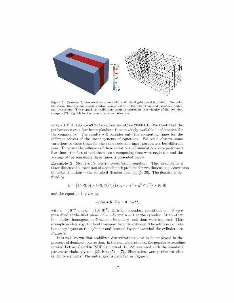
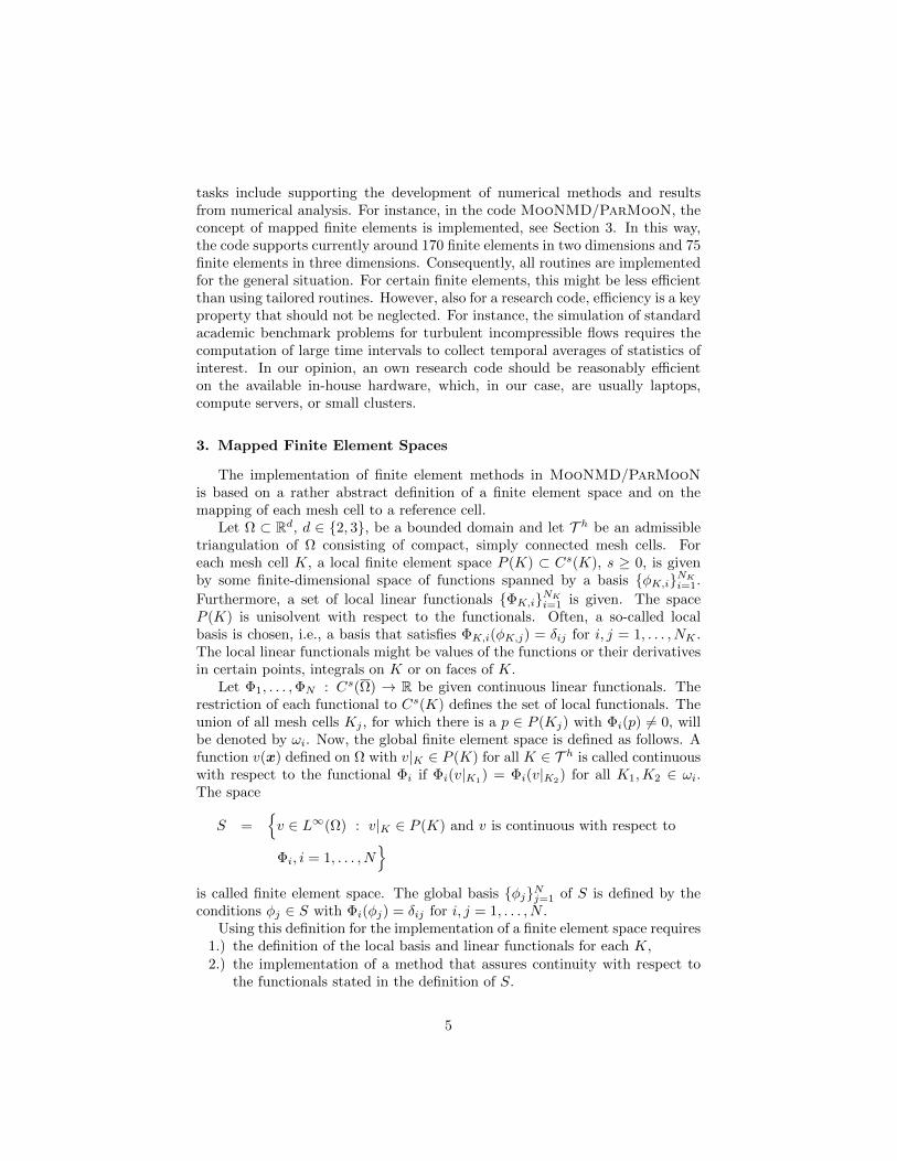
Figure 5: Example 2, numerical solution (left) and initial grid (level 0, right). The colorbar shows that the numerical solution computed with the SUPG method possesses under-and overshoots. These spurious oscillations occur in particular in a vicinity of the cylinder,compare [27, Fig. 14] for the two-dimensional situation.
servers HP BL460c Gen9 2xXeon, Fourteen-Core 2600MHz. We think that theperformance on a hardware platform that is widely available is of interest forthe community. The results will consider only the computing times for thedifferent solvers of the linear systems of equations. We could observe somevariations of these times for the same code and input parameters but differentruns. To reduce the influence of these variations, all simulations were performedfive times, the fastest and the slowest computing time were neglected and theaverage of the remaining three times is presented below.
Example 2: Steady-state convection-diffusion equation. This example is athree-dimensional extension of a benchmark problem for two-dimensional convection-diffusion equations – the so-called Hemker example [5, 20]. The domain is de-fined by
Ω =(−3, 9)× (−3, 3) \
(x, y) : x2 + y2 ≤ 1
× (0, 6)
and the equation is given by
−ε∆u+ b · ∇u = 0 in Ω,
with ε = 10−6 and b = (1, 0, 0)T . Dirichlet boundary conditions u = 0 wereprescribed at the inlet plane x = −3 and u = 1 at the cylinder. At all otherboundaries, homogeneous Neumann boundary conditions were imposed. Thisexample models, e.g., the heat transport from the cylinder. The solution exhibitsboundary layers at the cylinder and internal layers downwind the cylinder, seeFigure 5.
It is well known that stabilized discretizations have to be employed in thepresence of dominant convection. In the numerical studies, the popular streamline-upwind Petrov–Galerkin (SUPG) method [12, 22] was used with the standardparameter choice given in [26, Eqs. (5) – (7)]. Simulations were performed withQ1 finite elements. The initial grid is depicted in Figure 5.
17

2 4 8 12 16 20 24
# processors
0
500
1000
1500
2000
2500
3000
3500solver time in sec.
FGMRES + SSOR (PETSc)
FGMRES + AMG (PETSc)
FGMRES + MG (ParMooN)
MUMPS
2 4 8 12 16 20 24
# processors
10
20
30
40
50
60
70
80
90
solver time in sec.
FGMRES + SSOR (PETSc)
FGMRES + AMG (PETSc)
FGMRES + MG (ParMooN)
Figure 6: Example 2, solver times on refinement level 4.
2 4 8 12 16 20 24
# processors
100
200
300
400
500
600
solver time in sec.
FGMRES + SSOR (PETSc)
FGMRES + MG (ParMooN)
Figure 7: Example 2, solver times on refinement level 5. PETSc FGMRES with BoomerAMGconverged only with two processors (1519 sec.).
Computational results are presented in Figures 6 and 7 for refinement lev-els 4 (1 297 375 d.o.f.s) and 5 (10 388 032 d.o.f.s). The PETSc solvers werecalled with the flags -ksp type fgmres -pc type sor and -ksp type fgmres
-pc type hypre -pc hypre type boomeramg, respectively. For the geometricmultigrid preconditioner, the V(2,2)-cycle was used and the overrelaxation pa-rameter of the SSOR smoother within the block-Jacobi method was set to beω = 1. This approach is certainly not optimal since with an increasing numberof processes the number of blocks of the block-Jacobi method increases, whichin turn makes it advantageous to apply some damping, i.e., a somewhat smalleroverrelaxation parameter. In order not to increase the complexity of the numer-ical studies, we decided to fix a constant overrelaxation parameter that workedreasonably well for the whole range of processor numbers which was used. Theiterative solvers were stopped if the Euclidean norm of the residual vector wasless than 10−10. Parameters like the stopping criterion, the overrelaxation fac-tor, and the restart parameter were the same in all iterative methods.
18

It can be seen in Figure 6 that the sparse direct solver performed less effi-cient by around two orders of magnitude than the other solvers. This behav-ior was observed for all studied scalar problems and no further results withthis solver for scalar problems will be presented. Among the iterative solvers,PETSc FGMRES with SSOR preconditioner and ParMooN FGMRES withgeometric multigrid preconditioner (MG) performed notably more efficient thanPETSc FGMRES with BoomerAMG. The latter solver did not even convergeon the finer grid in the simulations on more than two processors. With re-spect to the computing times and the stability, similar results were obtained byapplying two V(1,1) BoomerAMG cycles (-pc hypre boomeramg max iter 2).With the V(2,2) cycle (-pc hypre boomeramg grid sweeps all 2), the solverdid not converge. FGMRES with SSOR required considerably more iterationsthan ParMooN FGMRES with MG: around 125 vs. 25 on level 4 and 320vs. 45 on level 5. A notable decrease of the computing time for the iterativesolvers on the coarser grid can be observed only until 8 processors. On this grid,PETSc FGMRES with SSOR was a little bit faster than ParMooN FGMRESwith MG. On the finer grid, a decrease of the computing times occurred until16 processors and ParMooN FGMRES with MG was often a little bit moreefficient.
Example 3: Time-dependent convection-diffusion-reaction equation. This ex-ample can be found also in the literature, e.g., in [29], and it models a typicalsituation which is encountered in applications. A species enters the domainΩ = (0, 1)3 at the inlet Γin = 0 × (5/8, 6/8)× (5/8, 6/8) and it is transportedthrough the domain to the outlet Γout = 1 × (3/8, 4/8) × (4/8, 5/8). In ad-dition, the species is diffused somewhat and in the subregion where the speciesis transported, also a reaction occurs. The ratio of diffusion and convection istypical for many applications.
The underlying model is given by
∂tu− ε∆u+ b · ∇u+ cu = 0 in (0, 3)× Ω,
u = uin in (0, 3)× Γin,
ε∂u
∂n= 0 on (0, 3)× ΓN,
u = 0 on (0, 3)× (∂Ω \ (ΓN ∪ Γin)) ,
u(0, ·) = u0 in Ω.
The diffusion parameter is given by ε = 10−6, the convection field is defined byb = (1,−1/4,−1/8)T , and the reaction by
c(x) =
1 if dist(x, g) ≤ 0.1,
0 else,
where g is the line through the center of the inlet and the center of the outletand dist(x, g) denotes the Euclidean distance of the point x to the line g. The
19

2 4 8 12 16 20 24
# processors
500
1000
1500
2000solver time in sec.
FGMRES + SSOR (PETSc)
FGMRES + AMG (PETSc)
FGMRES + MG (ParMooN)
2 4 8 12 16 20 24
# processors
40
60
80
100
120
140
solver time in sec.
FGMRES + SSOR (PETSc)
FGMRES + MG (ParMooN)
Figure 8: Example 3, solver times on the 643 cubed mesh.
boundary condition at the inlet is prescribed by
uin =
sin(πt/2) if t ∈ [0, 1],
1 if t ∈ (1, 2],
sin(π(t− 1)/2) if t ∈ (2, 3].
The initial condition is set to be u0(x) = 0. Initially, in the time interval [0, 1],the inflow increases and the injected species is transported towards the outlet.Then, there is a constant inflow in the time interval (1, 2] and the species reachesthe outlet. At t = 2, there is almost a steady-state solution. Finally, the inflowdecreases in the time interval (2, 3], compare [29].
The SUPG stabilization of the Q1 finite element method was used and astemporal discretization, the Crank–Nicolson scheme with the equidistant timestep ∆t = 10−2 was applied. Simulations were performed on grids with 643 and1283 cubic mesh cells. The coarsest grid for the geometric multigrid methodpossessed 43 cubic mesh cells. The SSOR method was applied with the over-relaxation parameter ω = 1.25. As initial guess for the iterative solvers, thesolution from the previous discrete time was used. The availability of a goodinitial guess and the dominance of the system matrix by the mass matrix arethe main differences to the steady-state case.
Computing times for the iterative solvers are presented in Figures 8 and 9.On the coarser grid, a speed-up can be observed only until 8 processors andon the finer grid until 12 to 16 processors. With respect to the efficiency ofthe iterative solvers, the same observations can be made as in the steady-stateExample 2. Using the V(2,2) cycle or two V(1,1) cycles in the BoomerAMGgave the same order of computing times as the presented times of the V(1,1)cycle. The same statement holds true for the number of iterations per time step,e.g., on the finer grid there were up to 45 for PETSc FGMRES with SSOR andaround 1-3 for PETSc FGMRES with BoomerAMG and ParMooN FGMRESwith MG.
Example 4: Steady-state incompressible Navier–Stokes equations. This exam-
20
2 4 8 12 16 20 24
# processors
5000
10000
15000
20000
solver time in sec.
FGMRES + SSOR (PETSc)
FGMRES + AMG (PETSc)
FGMRES + MG (ParMooN)
2 4 8 12 16 20 24
# processors
400
600
800
1000
1200
1400
1600
solver time in sec.
FGMRES + SSOR (PETSc)
FGMRES + MG (ParMooN)
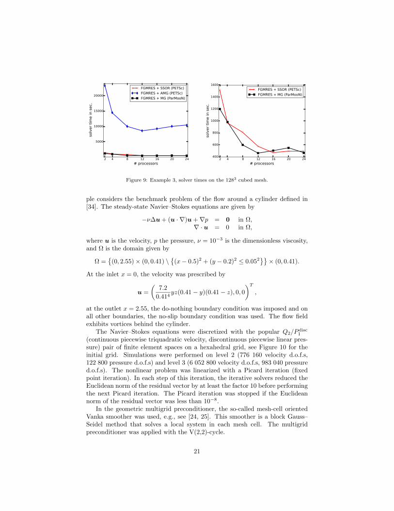
Figure 9: Example 3, solver times on the 1283 cubed mesh.
ple considers the benchmark problem of the flow around a cylinder defined in[34]. The steady-state Navier–Stokes equations are given by
−ν∆u + (u · ∇)u +∇p = 0 in Ω,∇ · u = 0 in Ω,
where u is the velocity, p the pressure, ν = 10−3 is the dimensionless viscosity,and Ω is the domain given by
Ω =
(0, 2.55)× (0, 0.41) \
(x− 0.5)2 + (y − 0.2)2 ≤ 0.052× (0, 0.41).
At the inlet x = 0, the velocity was prescribed by
u =
(7.2
0.414yz(0.41− y)(0.41− z), 0, 0
)T
,
at the outlet x = 2.55, the do-nothing boundary condition was imposed and onall other boundaries, the no-slip boundary condition was used. The flow fieldexhibits vortices behind the cylinder.
The Navier–Stokes equations were discretized with the popular Q2/Pdisc1
(continuous piecewise triquadratic velocity, discontinuous piecewise linear pres-sure) pair of finite element spaces on a hexahedral grid, see Figure 10 for theinitial grid. Simulations were performed on level 2 (776 160 velocity d.o.f.s,122 800 pressure d.o.f.s) and level 3 (6 052 800 velocity d.o.f.s, 983 040 pressured.o.f.s). The nonlinear problem was linearized with a Picard iteration (fixedpoint iteration). In each step of this iteration, the iterative solvers reduced theEuclidean norm of the residual vector by at least the factor 10 before performingthe next Picard iteration. The Picard iteration was stopped if the Euclideannorm of the residual vector was less than 10−8.
In the geometric multigrid preconditioner, the so-called mesh-cell orientedVanka smoother was used, e.g., see [24, 25]. This smoother is a block Gauss–Seidel method that solves a local system in each mesh cell. The multigridpreconditioner was applied with the V(2,2)-cycle.
21

Figure 10: Example 4, initial grid (level 0).
2 4 8 12 16 20 24
# processors
0
10000
20000
30000
40000
50000
solver time in sec.
FGMRES + LSC (PETSc)
FGMRES + MG (ParMooN)
MUMPS
2 4 8 12 16 20 24
# processors
50
100
150
200
250
300
350
solver time in sec.
FGMRES + MG (ParMooN)
Figure 11: Example 4, solver times on refinement level 2.
The linearization and used discretization of the incompressible Navier–Stokesequations require the solution of a linear saddle point problem in each Picarditeration. We tried several options for calling an iterative solver from PETScfor such problems, as well based on the coupled system as on Schur complementapproaches. Only with a Schur complement approach and the least squarecommutator (LSC) preconditioner (-ksp type fgmres -pc type fieldsplit
-pc fieldsplit type schur -pc fieldsplit schur factorization type upper
-fieldsplit 1 pc type lsc -fieldsplit 1 lsc pc type lu -fieldsplit 0 ksp type
preonly -fieldsplit 0 pc type lu), reasonable computing times could beobtained, at least for the coarser grid, see Figure 11. Like for the scalar prob-lems, the sparse direct solver performed by far the least efficient. The solverwith the geometric multigrid method was more efficient by around a factor of20 compared with the iterative solver called from PETSc. For the finer grid,the numerical studies were restricted to the geometric multigrid preconditioner,see Figure 12. It can be observed that increasing the number of processors from2 to 20 reduces the computing time by a factor of around 6.6.
22

2 4 8 12 16 20 24
# processors
500
1000
1500
2000so
lver tim
e in s
ec.
FGMRES + MG (ParMooN)
2 4 8 12 16 20 24
# processors
0.5
0.6
0.7
0.8
0.9
1.0
scalin
g
Figure 12: Example 4, solver times and scaling on refinement level 3. The scaling is computedby 2 · t2/(p · tp), where p is the number of processors and tp the corresponding time from theleft picture.
7. Summary
This paper presented some aspects of the remanufacturing of an existing re-search code, in particular with respect to its parallelization. All distinct featuresof the predecessor code could be incorporated in a straightforward way into themodernized code ParMooN. The efficiency of the most complex method in theparallel implementation, the geometric multigrid method, was assessed againstsome parallel solvers that are available in external libraries. The major con-clusions of this assessment are twofold. For scalar convection-diffusion-reactionequations, the geometric multigrid preconditioner was similarly efficient as aniterative solver from the PETSc library. The larger the problems became, thebetter was its efficiency in comparison with the external solver. For linear saddlepoint problems, arising in the simulation of the incompressible Navier–Stokesequations, we could not find so far any external solver that proved to be nearlyas efficient as the geometric multigrid preconditioner.
On the one hand, we keep on working at improving the efficiency of the ge-ometric multigrid preconditioner. On the other hand, we continue to assess ex-ternal libraries with respect to efficient solvers for linear saddle point problems,which can be used in situations where a multigrid hierarchy is not available. Inaddition, an assessment as presented in this paper on another widely availablehardware platform, namely small clusters of processors, is planned.
References
[1] James Ahrens, Berk Geveci, and Charles Law. ParaView: An End-UserTool for Large Data Visualization. Visualization Handbook. Elsevier, 2005.
[2] Martin Alns, Jan Blechta, Johan Hake, August Johansson, BenjaminKehlet, Anders Logg, Chris Richardson, Johannes Ring, Marie Rognes,
23

and Garth Wells. The fenics project version 1.5. Archive of NumericalSoftware, 3(100), 2015.
[3] Patrick R. Amestoy, Iain S. Duff, Jean-Yves L’Excellent, and Jacko Koster.A fully asynchronous multifrontal solver using distributed dynamic schedul-ing. SIAM J. Matrix Anal. Appl., 23(1):15–41 (electronic), 2001.
[4] Patrick R. Amestoy, Abdou Guermouche, Jean-Yves L’Excellent, andStephane Pralet. Hybrid scheduling for the parallel solution of linear sys-tems. Parallel Comput., 32(2):136–156, 2006.
[5] Matthias Augustin, Alfonso Caiazzo, Andre Fiebach, Jurgen Fuhrmann,Volker John, Alexander Linke, and Rudolf Umla. An assessment of dis-cretizations for convection-dominated convection-diffusion equations. Com-put. Methods Appl. Mech. Engrg., 200(47-48):3395–3409, 2011.
[6] Utkarsh Ayachit. The ParaView Guide: A Parallel Visualization Applica-tion. Kitware, Inc., 2015.
[7] Satish Balay, Shrirang Abhyankar, Mark F. Adams, Jed Brown, PeterBrune, Kris Buschelman, Lisandro Dalcin, Victor Eijkhout, William D.Gropp, Dinesh Kaushik, Matthew G. Knepley, Lois Curfman McInnes, KarlRupp, Barry F. Smith, Stefano Zampini, Hong Zhang, and Hong Zhang.PETSc Web page. http://www.mcs.anl.gov/petsc, 2016.
[8] Satish Balay, Shrirang Abhyankar, Mark F. Adams, Jed Brown, PeterBrune, Kris Buschelman, Lisandro Dalcin, Victor Eijkhout, William D.Gropp, Dinesh Kaushik, Matthew G. Knepley, Lois Curfman McInnes, KarlRupp, Barry F. Smith, Stefano Zampini, Hong Zhang, and Hong Zhang.PETSc users manual. Technical Report ANL-95/11 - Revision 3.7, ArgonneNational Laboratory, 2016.
[9] Satish Balay, William D. Gropp, Lois Curfman McInnes, and Barry F.Smith. Efficient management of parallelism in object oriented numericalsoftware libraries. In E. Arge, A. M. Bruaset, and H. P. Langtangen, editors,Modern Software Tools in Scientific Computing, pages 163–202. BirkhauserPress, 1997.
[10] W. Bangerth, D. Davydov, T. Heister, L. Heltai, G. Kanschat, M. Kron-bichler, M. Maier, B. Turcksin, and D. Wells. The deal.II library, version8.4. Journal of Numerical Mathematics, 24, 2016.
[11] Markus Blatt, Ansgar Burchardt, Andreas Dedner, Christian Engwer, Jor-rit Fahlke, Bernd Flemisch, Christoph Gersbacher, Carsten Graser, FelixGruber, Christoph Gruninger, Dominic Kempf, Robert Klofkorn, TobiasMalkmus, Steffen Muthing, Martin Nolte, Marian Piatkowski, and OliverSander. The distributed and unified numerics environment, version 2.4.Archive of Numerical Software, 4(100):13–29, 2016.
24

[12] Alexander N. Brooks and Thomas J. R. Hughes. Streamlineupwind/Petrov-Galerkin formulations for convection dominated flows withparticular emphasis on the incompressible Navier-Stokes equations. Com-put. Methods Appl. Mech. Engrg., 32(1-3):199–259, 1982.
[13] Alfonso Caiazzo, Volker John, and Ulrich Wilbrandt. On classical itera-tive subdomain methods for the Stokes-Darcy problem. Comput. Geosci.,18(5):711–728, 2014.
[14] Philippe G. Ciarlet. The finite element method for elliptic problems. North-Holland Publishing Co., Amsterdam, 1978. Studies in Mathematics and itsApplications, Vol. 4.
[15] Andreas Dedner, Robert Klofkorn, Martin Nolte, and Mario Ohlberger. Ageneric interface for parallel and adaptive discretization schemes: abstrac-tion principles and the DUNE-FEM module. Computing, 90(3-4):165–196,2010.
[16] Howard C. Elman, Alison Ramage, and David J. Silvester. IFISS: a compu-tational laboratory for investigating incompressible flow problems. SIAMRev., 56(2):261–273, 2014.
[17] Howard C. Elman, David J. Silvester, and Andrew J. Wathen. Finiteelements and fast iterative solvers: with applications in incompressible fluiddynamics. Numerical Mathematics and Scientific Computation. OxfordUniversity Press, Oxford, second edition, 2014.
[18] S. Ganesan, V. John, G. Matthies, R. Meesala, S. Abdus, and U. Wilbrandt.An object oriented parallel finite element scheme for computing pdes: De-sign and implementation. In IEEE 23rd International Conference on HighPerformance Computing Workshops (HiPCW) Hyderabad, pages 106–115.IEEE, 2016.
[19] F. Hecht. New development in freefem++. J. Numer. Math., 20(3-4):251–265, 2012.
[20] P. W. Hemker. A singularly perturbed model problem for numerical com-putation. J. Comput. Appl. Math., 76(1-2):277–285, 1996.
[21] Van Emden Henson and Ulrike Meier Yang. BoomerAMG: a parallel alge-braic multigrid solver and preconditioner. Appl. Numer. Math., 41(1):155–177, 2002.
[22] T. J. R. Hughes and A. Brooks. A multidimensional upwind scheme withno crosswind diffusion. In Finite element methods for convection dominatedflows (Papers, Winter Ann. Meeting Amer. Soc. Mech. Engrs., New York,1979), volume 34 of AMD, pages 19–35. Amer. Soc. Mech. Engrs. (ASME),New York, 1979.
25

[23] S. Hysing, S. Turek, D. Kuzmin, N. Parolini, E. Burman, S. Ganesan,and L. Tobiska. Quantitative benchmark computations of two-dimensionalbubble dynamics. Internat. J. Numer. Methods Fluids, 60(11):1259–1288,2009.
[24] Volker John. Higher order finite element methods and multigrid solversin a benchmark problem for the 3D Navier-Stokes equations. Internat. J.Numer. Methods Fluids, 40(6):775–798, 2002.
[25] Volker John. Finite Element Methods for Incompressible Flow Problems,volume 51 of Springer Series in Computational Mathematics. Springer-Verlag, Berlin, 2016.
[26] Volker John and Petr Knobloch. On spurious oscillations at layers di-minishing (SOLD) methods for convection-diffusion equations. I. A review.Comput. Methods Appl. Mech. Engrg., 196(17-20):2197–2215, 2007.
[27] Volker John, Petr Knobloch, and Simona B. Savescu. A posteriori op-timization of parameters in stabilized methods for convection-diffusionproblems—Part I. Comput. Methods Appl. Mech. Engrg., 200(41-44):2916–2929, 2011.
[28] Volker John and Gunar Matthies. MooNMD—a program package based onmapped finite element methods. Comput. Vis. Sci., 6(2-3):163–169, 2004.
[29] Volker John and Julia Novo. On (essentially) non-oscillatory discretiza-tions of evolutionary convection-diffusion equations. J. Comput. Phys.,231(4):1570–1586, 2012.
[30] George Karypis and Vipin Kumar. MeTis: Unstructured Graph Partition-ing and Sparse Matrix Ordering System, Version 4.0. http://www.cs.umn.edu/~metis, 2009.
[31] MPI-Forum. Mpi: A message-passing interface standard, version 3.1. Tech-nical report, University of Tennessee, Knoxville, Tennessee, June 2015.
[32] OpenFOAM. OpenFOAM Web page. http://openfoam.org/, 2016.
[33] Youcef Saad. A flexible inner-outer preconditioned GMRES algorithm.SIAM J. Sci. Comput., 14(2):461–469, 1993.
[34] M. Schafer and S. Turek. Benchmark computations of laminar flow arounda cylinder. (With support by F. Durst, E. Krause and R. Rannacher). InFlow simulation with high-performance computers II. DFG priority researchprogramme results 1993 - 1995, pages 547–566. Wiesbaden: Vieweg, 1996.
[35] F. Schieweck. A general transfer operator for arbitrary finite elementspaces. Preprint 00-25, Fakultat fur Mathematik, Otto-von-Guericke-Universitat Magdeburg, 2000.
26

[36] Ellen Schmeyer, Robert Bordas, Dominique Thevenin, and Volker John.Numerical simulations and measurements of a droplet size distribution ina turbulent vortex street. Meteorol. Z., 23(4):387–396, 09 2014.
[37] Scopus. https://www.scopus.com/record/display.uri?src=s&origin=cto&ctoId=CTODS 701493876&stateKey=CTOF 701493878&eid=2-s2.0-7444244347. accessed 13.09.2016.
27