Embed Size (px)
Citation preview
France
rentialspect toals withme are
ulationntifica-ation
arisingcation
9nd
Applied Numerical Mathematics 54 (2005) 519–536www.elsevier.com/locate/apnum
Parameter identification for chemical modelsin combustion problems
R. Beckera, M. Braackb,∗, B. Vexlerb
a Laboratoire de Mathematiques Appliquees, Université de Pau et des Pays de l’Adour, BP 1155, 64013 Pau cedex,b Institute of Applied Mathematics, University of Heidelberg, INF 294, 69120 Heidelberg, Germany
Abstract
We present an algorithm for parameter identification in combustion problems modeled by partial diffeequations. The method includes local mesh refinement controlled by a posteriori error estimation with rethe error in the parameters. The algorithm is applied to two types of combustion problems. The first one dethe identification of Arrhenius parameters, while in the second one diffusion coefficients for an ozone flacalibrated. 2004 IMACS. Published by Elsevier B.V. All rights reserved.
1. Introduction
Estimation of the unknown parameters in chemical models is indispensable for successful simand optimization of combustion problems. In this paper we present an algorithm for parameter idetion in the context of multidimensional reactive flows. Typical problems are, for instance, the estimof reaction rates or Arrhenius parameters and the estimation of diffusion coefficients. Since thesystem of partial differential equations is usually very complex, the solution of parameter identifi
This work has been supported by the German Research Foundation (DFG), through theSonderforschungsbereich 35‘Reactive Flows, Diffusion and Transport’, and theGraduiertenkolleg‘Complex Processes: Modeling, Simulation aOptimization’ at the Interdisciplinary Center of Scientific Computing (IWR), University of Heidelberg.* Corresponding author.
E-mail addresses:[email protected] (R. Becker), [email protected] (M. Braack),
[email protected] (B. Vexler).0168-9274/$30.00 2004 IMACS. Published by Elsevier B.V. All rights reserved.doi:10.1016/j.apnum.2004.09.017
520 R. Becker et al. / Applied Numerical Mathematics 54 (2005) 519–536
esentedation.
educinge opti-ementa suffi-teps arereplace
ncludesultigrid
tionary
type
tor-ertain,f Arrhe-which
and itshe firstove (2).view ofis [14].ationsated, for
lem ashere-of therror es-cientses theelemen-rder to-iments.
problems requires development of special discretization and optimization techniques. In the pralgorithm we use local mesh refinement for finding efficient discretizations for parameter identificThe approach is based on a posteriori error estimation for the error in parameters and allows for rthe dimension of the discretized problem to a minimum for achieving a prescribed accuracy. Thmization loop for determining the unknown parameters is intrinsically coupled with the mesh refinalgorithm: at the beginning, the optimization algorithm acts on coarse meshes. After achievingcient reduction of the cost functional the mesh is refined and the optimization continues. These siterated until the estimated error in parameters is below a user-specified tolerance. This allows tooptimization iterations on fine meshes by iterations on coarse meshes. In addition, our algorithm ithe use of stabilized finite element discretizations on hierarchies of locally refined meshes, a mprocedure for solving the linear sub-problems, and a special optimization loop.
For discussing the subject, we consider the following simple model problem of a scalar staconvection–diffusion–reaction equation (cdr-equation) for the variableu in a domainΩ ⊂ R
2 with adivergence-free vector fieldβ and a diffusion coefficientD:
β · ∇u − div(D∇u) + s(u, q) = f, (1)
provided with Dirichlet boundary conditionsu = u at the inflow boundaryΓin ⊂ ∂Ω and Neumannconditions∂nu = 0 on∂Ω \Γin. As usual in combustion problems, the reaction term is of Arrhenius
s(u, q) := Aexp−E/(d − u)
u(c − u). (2)
While d, c are fixed parameters, the parametersA, E are considered as unknown and form the vecvalued parameterq = (A,E) ∈ R
2. Since they are not directly measurable, we assume to have cmeasurementsC ∈ R
nm , which should match with computed quantitiesC(u) ∈ Rnm . Here we may think
e.g., of laser measurements of mean concentrations along fixed lines, see Section 5. Calibration onius parameter has be done by many scientists, for instance, by Lohmann [18] for coal pyrolysisis frequently used in chemical engineering.
The aim of this work is the presentation of the numerical background of the proposed methodvalidation by model problems. To this end numerical results for two test problems are presented. Tone deals with the estimation of Arrhenius parameters for one single reaction, as mentioned abIn the second example we analyze diffusion parameters in a combustion problem. For an overparameter estimation problems in chemistry, we refer to the book of Englezos and KalogerakTherein, many applications of parameter identification in the framework of ordinary differential equare given. Parameter estimation problems for reactive flows in one space dimensions are treinstance, by Bock et al. [20].
This paper is organized as follows. In Section 2 we formulate the parameter identification proban optimization problem and describe the optimization algorithm for it on the continuous level. Tafter, in Section 3 the optimization loop is applied to the stabilized finite element discretizationproblem. Section 4 is devoted to the adaptive mesh refinement algorithm and the a posteriori etimation. In Section 5, the described algorithms are applied for estimating the Arrhenius coeffiof the scalar cdr-equation (1). A more complex ozone flame is analyzed in Section 6. It includequations for compressible flows, a system of cdr-equations for three chemical species and 6tary (bi-directional) reactions. The considered parameters calibrate a simple diffusion model in omatch with given observations. In both examples, the measurementsC are produced numerically. In future work, the whole approach will be applied to examples with measured data coming from exper
R. Becker et al. / Applied Numerical Mathematics 54 (2005) 519–536 521
rame-cationuous
ert
nsf
for
he cost
)
[13],
ith the
2. The optimization algorithm for parameter identification problems
The aim of this section is the description of the optimization algorithms for the solution of the pater identification problems. In Section 2.1, we start with the formulation of the parameter identifiproblem in variational form and describe the typical optimization algorithms for it on the continlevel including trust-region techniques.
2.1. The optimization algorithm for the continuous problem
We consider the parameter identification problem in the following variational form: thestate variableu is supposed to be a sum of the functionu describing the Dirichlet conditions and a function of a HilbspaceV , i.e.,u ∈ V := u + V . The unknown parameterq is assumed to be in the spaceQ := R
np . Thesystem of equations for the state variableu reads
a(u, q)(φ) = (f,φ) ∀φ ∈ V, (3)
wherea(u, q)(φ) is a form acting on the function spaceV × Q × V . This form is linear inφ and maybe nonlinear inu andq. The right sidef is assumed to be in the dual spaceV ′. The forma(u, q)(φ) isassumed to be differentiable with respect tou andq with Gateaux derivativesa′
u anda′q , respectively.
For the cdr-equation (1) the forma(u, q)(φ) is obtained by multiplication of Eq. (1) with test functioφ ∈ V = v ∈ H 1(Ω)|vΓin = 0, integration over the computational domainΩ and integration by parts othe diffusive term. The resulting discrete Galerkin form is
a(u, q)(φ) :=∫Ω
(β · ∇u + s(u, q)
)φ dx +
∫Ω
D∇u∇φ dx. (4)
Further, the measurable quantities are represented by a linear observation operatorC : V → Z, whichmaps the state variableu into the space of measurementsZ := R
nm with nm np. We denote by〈· , ·〉Zthe Euclidean scalar product ofZ and by‖ · ‖Z the corresponding norm. Similar notations are usedthe scalar product and norm in the spaceQ.
The values of the parameters are estimated from a given set of measurementsC ∈ Z using a least-squares approach, in such a way that we obtain the constrained optimization problem with tfunctionalJ : V → R:
Minimize J (u) := 1
2
∥∥C(u) − C∥∥2
Z, under the constraint (3). (5
Under a regularity assumption fora′u, the implicit function theorem in Banach spaces, see Dieudonné
implies the existence of an open setQ0 ⊂ Q, containing the optimal parameterq, and a continuouslydifferentiable solution operatorS :Q0 → V , q → S(q), so that (3) is fulfilled foru = S(q). Using thissolution operatorS, we define the reduced observation operatorc :Q0 → Z by c(q) := C(S(q)), in or-der to reformulate the problem under consideration as an unconstrained optimization problem wreduced cost functionalj :Q0 → R:
Minimize j (q) := 1∥∥c(q) − C∥∥2
, q ∈ Q . (6)
2 Z 0
522 R. Becker et al. / Applied Numerical Mathematics 54 (2005) 519–536
-
ely.
f theing
as the
tors, re-
t right
ed
Vexlernis and
Denoting byG = c′(q) the Jacobian matrix of the reduced observation operatorc, the first-order necessary conditionj ′(q) = 0 for (6) reads
G∗(c(q) − C) = 0, (7)
whereG∗ denotes the transpose ofG. The unconstrained optimization problem (6) is solved iterativStarting with an initial guessq0, the next parameter is obtained byqk+1 = qk + δq, where the updateδqis the solution of the problem
Hkδq = G∗krk, whererk := C − c
(qk
), Gk := c′(qk
), (8)
and Hk is an approximation of the Hessian∇2j (qk) of the reduced cost functionalj . Although δq
depends on the iteratek, we suppress the index in order to facilitate the readability. The choice omatrix Hk ∈ R
np×np leads to different variants of the optimization algorithm. We consider the followtypical possibilities:
2.1.1. Gauß–Newton algorithmThe choiceHk := G∗
kGk corresponds to the Gauß–Newton algorithm, which can be interpretedsolution to the linearized minimization problem
Minimize1
2
∥∥c(qk
) + Gkδq − C∥∥2
. (9)
The componentsGij of the JacobianGk can be computed as follows:
Gij := ∂ci
∂qj
(qk
) = Ci(wj ), i = 1, . . . , nm, j = 1, . . . , np,
whereCi andci denote the components of the observation and the reduced observation operaspectively. The tanget solutionwj ∈ V is determined by
a′u
(uk, qk
)(wj ,φ) = −a′
qj
(uk, qk
)(φ) ∀φ ∈ V, j = 1, . . . , np, (10)
whereuk = S(qk). For one Gauß–Newton step, the state equation (3) foruk = S(qk) andnp tangentproblems (10) have to be solved which originate from the same linear operator but with differensides. The solution of (8) is uncritical due to the small dimension ofHk. Note that we suppress the indexk
for the matrix entriesGij and the vectorswj .
2.1.2. Full Newton algorithmAnother possibility is to setHk := ∇2j (qk), which leads to the full Newton algorithm. The requir
Hessian∇2j (qk) is given by
∇2j(qk
) = G∗kGk + Mk. (11)
As before, the computation of the JacobianGk is required. The entries of the matrixMk ∈ Rnp×np can be
computed by a subtle evaluation of several second derivatives of the forma(u, q)(φ) in the directionswj
(the solutions of the tangent problems (10)) andz ∈ V , the solution of the adjoint equation
a′u
(uk, qk
)(φ, z) = −(rk,Cφ) ∀φ ∈ V. (12)
Since we do not use this method for the problems under consideration, we refer to Becker and[4] for details. For convergence theory of Gauß–Newton and Newton methods see, e.g., DenSchnabel [11] or Nocedal and Wright [19].
R. Becker et al. / Applied Numerical Mathematics 54 (2005) 519–536 523
er-uadratic
r evenost of
the
ian.orithmrations.
initial-hortly
ntc-a
the
t-regionoice one
For large least-squares residuals‖C(u)− C‖Z, the Gauß–Newton algorithm often shows slow convgence. The full Newton algorithm has better (local) convergence properties, because it leads to qconvergence. However, for reactive flow problems, the evaluation of the second derivatives ofa(u, q)(φ)
is usually very expensive. Therefore, the use of the full Newton algorithms is often unattractive, oimpossible. We discuss shortly an alternative algorithm which combines the comparative “low” cthe Gauß–Newton method and the better convergence properties of the full Newton.
2.1.3. Gauss–Newton-update methodBased on the ideas of Dennis et al. [12], we replace the expensive matrixMk in (11) by an approxi-
mation obtained by an update formula. It produces a sequence of computable matricesMk . Starting withM0 = 0:
Mk+1 = Mk + 1
y∗δq(xy∗ + yx∗) − x∗δq
(y∗δq)2yy∗,
wherey = G∗k+1 rk+1 −G∗
k rk, x = (G∗k+1 −G∗
k) rk+1 − Mkδq. Then, for the matrixHk we use the follow-ing Hessian approximation:Hk := G∗
kGk + Mk. Note, that no further equations have to be solved fordetermination ofMk .
The matricesMk are chosen in such a way thatHk is a secant approximation of the (exact) HessFor derivation and analysis of this update formula, see also [11]. In Section 6 we compare this algwith the Gauß–Newton method and observe a substantial difference in the required number of ite
2.2. Trust-region method
It is well known, that the convergence of the algorithms described so far is ensured, only if theguessq0 is in a sufficiently small neighborhood of the optimal parameterq. We use trust-region techniques in order to improve the global convergence, see, e.g., [11] or [19]. In the following, we sdescribe this algorithm. If the matrixHk is positive definite, the computation ofδq ∈ Q in (8) can beinterpreted as the solution of a minimization problem (cf. (9)):
Minimize mk(δq) := j(qk
) − r∗k Gkδq + 1
2δq∗Hkδq, δq ∈ Q. (13)
The cost functionalmk of (13) is the so-calledlocal model function, which behavior near the currepoint qk is similar to that of the actual cost functionalj defined in (6). However, the local model funtion mk may not be a good approximation ofj for large δq. Therefore, we restrict the search forminimizer ofmk to a ball (trust region) aroundqk. In other words, we replace the problem (13) byfollowing constrained optimization problem:
Minimize mk(δq), subject to‖δq‖Q ∆k, (14)
with a trust-region radius∆k to be determined iteratively.For the convergence properties of the trust-region method, the strategy for choosing the trus
radius∆k is crucial. Following the standard approach, see, e.g., Conn et al. [10], we base this chthe agreement between the model functionmk and the cost functionalj at the previous iteration. For thincrementδq, we define the ratio
ρk = j (qk) − j (qk + δq),
mk(0) − mk(δq)
524 R. Becker et al. / Applied Numerical Mathematics 54 (2005) 519–536
dtherink it,
to theyst
set
is
without
e easiestnt fine”estionsuniformesh re-ortant inn prob-ent. The
ned on
esh,nodes,
and use it as an indicator of the quality of the local modelmk. If this ratio is close to 1, there is a gooagreement between the modelmk and the cost functionalj for the current step. As a consequence,trust region is expanded for the next iteration. Otherwise, we do not alter the trust region or shdepending on the distance|ρk − 1|, see [19] for a precise definition.
The solution of the quadratic minimization problem (14) requires an additional remark. Duecompactness of the feasible set described by the condition‖δq‖Q ∆k, the problem (14) posses alwaa solution independently of the definiteness of the matrixHk. If the matrixHk is positive definite and iholds∥∥H−1
k G∗krk
∥∥Q
∆k,
we setδq = H−1k G∗
krk. Otherwise, the solutionδq is searched on the boundary of the feasibleδq|‖δq‖Q ∆k, and is determined by
δq = (Hk + λI)−1G∗krk,
whereI is the identity matrix andλ > 0 is chosen, such that‖δq‖Q = ∆k. For computation ofλ, thesingular value decomposition ofHk is computed andλ is determined by the scalar equation, whichsolved by one-dimensional Newton method, see, e.g., [19] for details.
For the numerical examples in Sections 5 and 6, the optimization algorithm does not convergeusing such globalization techniques.
3. The discretization by finite elements
The continuous state equation (3) and several tangent problems (10) have to be discretized. Thpossibility is to replace these equations by some numerical discrete approximations on a “sufficiemesh resulting from the uniform refinement of the starting mesh. However, the naturally arising quhere are: first, how to decide if a mesh is sufficient fine? Second, are the meshes produced by therefinement economical for the computation of parameters? And third, how to design another mfinement procedure in order to obtain more efficient meshes? These questions are extremely impcombustion problems, because of arising thin flame fronts. Furthermore, in parameter estimatiolems the measurements are usually local quantities which gives the need of local mesh refinemrequired procedure is described in Section 4.
3.1. Meshes and finite element spaces
For the discretization we use a conforming equal-order Galerkin finite element method defiquadrilateral meshesTh = K over the computational domainΩ ⊂ R
2, with cells denoted byK . Themesh parameterh is defined as a cell-wise constant function by settingh|K = hK andhK is the diameterof K . The straight parts which make up the boundary∂K of a cellK are calledfaces.
A meshTh is called regular, if it fulfills the standard conditions for shape-regular finite element msee, e.g., Ciarlet [8]. However, in order to easy the mesh refinement we allow the cell to havewhich lie on midpoints of faces of neighboring cells. But at most one suchhanging nodeis permitted foreach face.
R. Becker et al. / Applied Numerical Mathematics 54 (2005) 519–536 525
lled
mialsnson
m corre-intwise
s num-ues canom arouptetor
cribedmation
The discrete function spaceVh ⊂ V consist of continuous, piecewise polynomial functions (so-caQ1-elements) for all unknowns,
Vh = ϕh ∈ C(Ω); ϕh|K ∈ Q1
,
whereQ1 is the space of functions obtained by transformations of (isoparametric) bilinear polynoon a fixed reference unit cellK . For a detailed description of this standard construction, see [8] or Joh[17].
The case of hanging nodes requires some additional remarks. There are no degrees of freedosponding to these irregular nodes and the value of the finite element function is determined by pointerpolation. This implies continuity and therefore global conformity, i.e.,Vh ⊂ V . For implementationdetails, see, e.g., Carey and Oden [7].
For several applications, the Galerkin formulation is not stable. For instance, at higher Reynoldbers, advective terms become unstable. In order to overcome this limitation, stabilization techniqbe used. For this, the triangulationTh is supposed to be constructed in such a way that it results frcoarser quasi-regular meshT2h by one global refinement. By a “patch” of elements we denote a gof four cells inTh which results from a common coarser cell inT2h. The corresponding discrete finielement spacesV2h and Vh are nested:V2h ⊂ Vh. By I h
2h we denote the nodal interpolation operaI h
2h :Vh → V2h. By
πh :Vh → Vh, πhξ = ξ − I h2hξ
we denote the difference between the identity and this interpolation.
3.2. The stabilized nonlinear form
Let the discrete function spaces be given byVh ⊂ V , Vh := uh + Vh, with an approximationuh ofthe boundary datau. For fixed parameterqh ∈ Q, the discrete solutionuh ∈ Vh is determined by thediscretized state equation
ah(uh, qh)(φ) = (f,φ) ∀φ ∈ Vh. (15)
The nonlinear formah(uh, qh)(φ) results from a stabilized finite element discretization on the meshTh,given by a sum of the Galerkin part and stabilization terms:
ah(uh, qh)(φ) = a(uh, qh)(φ) + bh(uh, qh)(φ).
We note that the kind of the discretization is not essential for the discrete optimization loop desbelow. However, the use of finite elements is crucial for the derivation of the a posteriori error estiin Section 4.
3.2.1. Convection stabilizationFor a cdr-equation (1), the stabilization term added to the Galerkin formulation reads
bh(uh, qh)(φ) :=∑K∈Th
δK
∫K
(β · ∇πhuh)(β · ∇πhφ)dx, (16)
where the cell-wise coefficientsδK depend on the local balance of convection and diffusion:
δK := δ0h2K .
6D + hK‖β‖K
526 R. Becker et al. / Applied Numerical Mathematics 54 (2005) 519–536
d
added.t
e
ws en-nce they
iliza-
-on thestokes
d to the
r.
fer,
Here, the quantitieshK and‖β‖K are cell-wise values for the cell-size and the convectionβ. The para-meterδ0 is a fixed constant, usually chosen asδ0 = 0.5. Note, thatπh vanishes onV2h, and therefore, thestabilization vanishes for test functions of the coarse gridξ ∈ V2h. This type of stabilization is analyzeby Guermond [15].
For systems of cdr-equations, for each convective term, one stabilization term of type (16) isThe convectionβ and the particular diffusion coefficientD may depend itself fromu and may be differenfor each sub-equation.
3.2.2. Pressure-velocity stabilizationFor equal-order finite elements, the Galerkin formulation of the Stokes system for the pressurp and
velocity v,
divv = 0, −µ∆v + ∇p = f
is known to be unstable, since the stiff pressure-velocity coupling for (nearly) incompressible floforces spurious pressure modes. The same occurs for hydrodynamic incompressible flows siinvolve also the saddle-point structure of the Stokes system. Letph denote the discrete pressure,vh thediscrete velocity,uh = (ph, vh), andξ the test function for the divergence equation. The added stabtion term which damps acoustic pressure modes is of the form
bh(uh, qh)(φ) =∑K∈Th
αK
∫K
(∇πhph)(∇πhξ) dx, (17)
with weightsαK = α0h2K/µ depending on the mesh sizehK of cell K and the viscosityµ. The parame
ter α0 is usually chosen between 0.2 and 1. The stabilization term (17) acts as a diffusion termfine-grid scales of the pressure. The scaling proportional toh2
K give stability of the discrete equationand maintain accuracy. This type of stabilization is introduced in Becker and Braack [1] for the Sequation. Therein, a stability proof and an error analysis is given. The same stabilization is applie(compressible) Navier–Stokes equations.
The proposed stabilization is consistent in the sense that the introduced terms vanish forh → 0. Forsmooth solutions, the introduced perturbation is even of higher-order than the discretization erro
3.3. The finite-dimensional optimization algorithm
Analog to Section 2.1, we assume the regularity of the derivative(ah)′u, which implies the existence o
a discrete solution operatorSh, such thatuh = Sh(qh) fulfills the discrete state equation (15). Moreovwe introduce the discrete reduced observation operatorch by settingch(qh) = C(Sh(qh)). The optimiza-tion loop on a given meshTh for the problem
Minimize jh(qh) := 1
2
∥∥ch(qh) − C∥∥2
Z, qh ∈ Q,
starts with an initial guess for the parametersq0h ∈ Q. Thereafter, the corresponding discrete stateuk
h andthe next parameterqk+1
h are obtained by the discrete equations
ukh ∈ Vh: ah
(uk
h, qkh
)(φ) = (f,φ) ∀φ ∈ Vh,
δq ∈ Q: H δq = G∗r , r := C − c(qk
),
h h h h h h h h
R. Becker et al. / Applied Numerical Mathematics 54 (2005) 519–536 527
a-iscrete
d on theeasure
ntation
ß–
] for
velopedr whichul error
uence ofa given
efinesdure is
es fromization
qk+1h ∈ Q: qk+1
h = qkh + δqh, (18)
whereGh := c′h(q
kh) andHh the discrete approximation ofHk according the choice above. The globaliz
tion technique formulated for the continuous problems in Section 2.2 can be carried over to the dcase analogously.
4. Adaptive mesh refinement via a posteriori error estimation
In this section, we describe the adaptive algorithm for mesh refinement and error control basea posteriori error estimation for parameter identification problems developed in [4]. In order to mthe error in the parameters, we introduce an error functionalE :Q → R. The use of the error functionalE
allows to weight the relative importance of the different parameters. The following error represeholds:
E(q) − E(qh) = ηh + P + R. (19)
Here,ηh denotes the computable a posteriori error estimator given later. The remainder termR is due tolinearization and is cubic in the error. The termP appears if an inexact Newton algorithm (e.g., GauNewton) is applied. However,P vanishes if the optimal parameters perfectly match for (6), i.e.,j (q) = 0.Since the partsP andR are omitted in the numerical examples in this work, we simply refer to [4details.
The error estimator is based on the optimal control approach to a posteriori error estimation dein Becker and Rannacher [2,3]. However, a direct application of this approach leads to an estimatocontrols the error in the cost functional (5). In general, such an estimator does not provide usefbounds for the parameters, in contrast to the estimator (19) described in the following.
We sketch a generic adaptive mesh refinement algorithm. Such an algorithm generates a seqlocally refined meshes and corresponding finite element spaces until the estimated error is belowtoleranceTOL. For the following iteration, we have a mesh refinement procedure that adaptively ra given regular mesh to obtain a new regular mesh for the next iteration. The refinement proceguided by information based on the cell-wise contributions of the estimatorηh.
Adaptive mesh refinement algorithm1. Choose an initial meshTh0 and setl = 02. Construct the finite element spaceVhl
3. Compute the discrete optimalqhl∈ Q, i.e., iterate (18)
4. Evaluate the a posteriori error estimatorηhl
5. If ηhl TOL quit
6. RefineThl→ Thl+1 using information fromηhl
7. Incrementl and go to 2
In step 3 the least-squares problem is solved on a fixed mesh. As initial data we use the valuthe computation on the previous mesh. This allows us to avoid unnecessary iterations of the optimloop on fine meshes.
528 R. Becker et al. / Applied Numerical Mathematics 54 (2005) 519–536
the
define
sume.
lement
tion of, which
estima-in this
ctaack
lar cdr-le
s are aof ex-rameter
withor the
For evaluation of our a posteriori error estimatorηh, we consider an additional adjoint equation foradjoint variabley ∈ V :
a′u(u, q)(φ, y) = ⟨
G(G∗G
)−1∇E(q),C(φ)⟩Z
∀φ ∈ V, (20)
and solve the discrete version of it, i.e.,yh ∈ Vh:
(ah)′u(uh, qh)(φ, yh) = ⟨
Gh
(G∗
hGh
)−1∇E(qh),C(φ)⟩Z
∀φ ∈ Vh. (21)
We denote byρ andρ∗ the residuals of the state and the adjoint equations, respectively, i.e., wefor test functionsφ ∈ V :
ρ(uh)(φ) := (f,φ) − ah(uh, qh)(φ),
ρ∗(uh, yh)(φ) := ⟨Gh
(G∗
hGh
)−1∇E(qh),C(φ)⟩Z
− (ah)′u(uh, qh)(φ, yh).
Using this notation, the error estimator is given by
ηh = 1
2ρ(uh)(y − ihy) + 1
2ρ∗(uh, yh)(u − ihu), (22)
whereih :V → Vh is an appropriate interpolation operator, see Clément [9]. For simplicity we asthat uh = u, such thatu − ihu ∈ V . For a proof of (19) with the error estimator given by (22), see [4]
For evaluation of this error estimator, the local interpolation errorsy − ihy andu − ihu have to beapproximated. In our numerical examples, we use interpolation of the computed bilinear finite esolutionsyh anduh on the space of biquadratic finite elements on patches of cells.
The main computational cost for the a posteriori error estimator described above is the soluone auxiliary equation (21). This is cheap, even in comparison with only one Gauß–Newton stepincludes solution of the state (nonlinear) and of the several (linear) tangent equations.
These residual terms are still global quantities. In order to use it for local mesh adaptation, thetor ηh has still to be localized to cell-wise or node-wise error indicators. For the numerical resultswork, we perform node-wise localization by summation over all nodes of the mesh. For a meshTh withN nodes, the estimator can be expressed byηh = ∑N
i=1 τi . Then, the mesh is locally refined with respeto the error indicatorsηi := |τi |. For more details on the localization procedure used, we refer to Brand Ern [6]. However, there are also methods for localization to cell-wise quantities, see [3].
5. Identification of Arrhenius parameters
The first example we analyze with respect to the proposed optimization algorithm is the scaequation (1) withf ≡ 1, D = 10−6, and a chemical source term of Arrhenius type (2). The variabu
stands for the mole fraction of a fuel, while the mole fraction of the oxidizer is 0.2 − u. Since the Ar-rhenius law is a heuristic law and cannot be derived by physical laws, the involved parameterpriori unknown and have to be calibrated. This parameter fitting is usually done by comparisonperimental data and simulation results. Therefore, this example is well suited for the proposed paidentification algorithm.
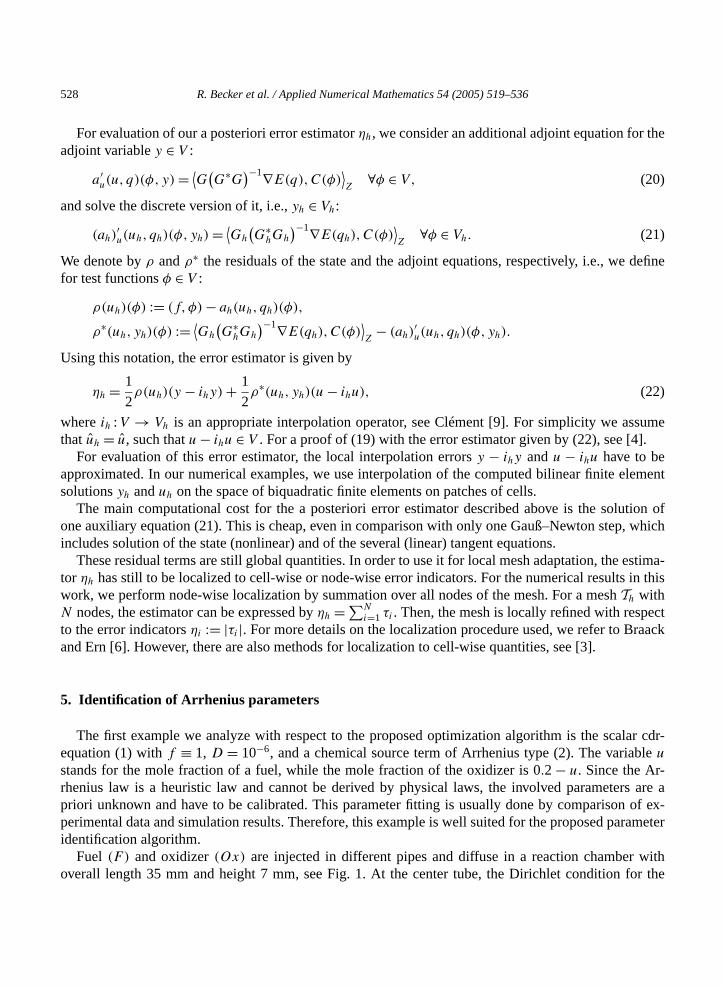
Fuel (F ) and oxidizer(Ox) are injected in different pipes and diffuse in a reaction chamberoverall length 35 mm and height 7 mm, see Fig. 1. At the center tube, the Dirichlet condition f
R. Becker et al. / Applied Numerical Mathematics 54 (2005) 519–536 529
atically
o-
ble
on
pu-ore
optimal
he
Fig. 1. Configuration of the reaction chamber for estimating Arrhenius coefficients. Dashed vertical lines indicate schemthe lines where the measurements are modeled.
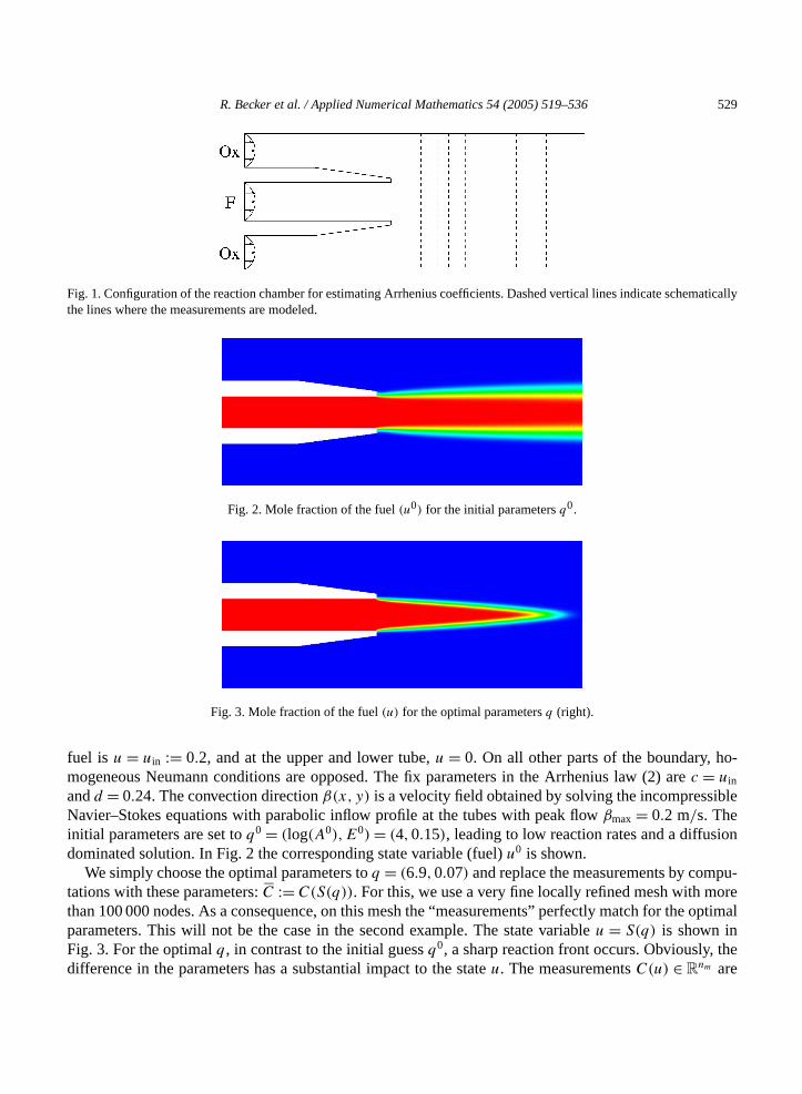
Fig. 2. Mole fraction of the fuel(u0) for the initial parametersq0.
Fig. 3. Mole fraction of the fuel(u) for the optimal parametersq (right).
fuel is u = uin := 0.2, and at the upper and lower tube,u = 0. On all other parts of the boundary, hmogeneous Neumann conditions are opposed. The fix parameters in the Arrhenius law (2) arec = uin
andd = 0.24. The convection directionβ(x, y) is a velocity field obtained by solving the incompressiNavier–Stokes equations with parabolic inflow profile at the tubes with peak flowβmax = 0.2 m/s. Theinitial parameters are set toq0 = (log(A0),E0) = (4,0.15), leading to low reaction rates and a diffusidominated solution. In Fig. 2 the corresponding state variable (fuel)u0 is shown.
We simply choose the optimal parameters toq = (6.9,0.07) and replace the measurements by comtations with these parameters:C := C(S(q)). For this, we use a very fine locally refined mesh with mthan 100 000 nodes. As a consequence, on this mesh the “measurements” perfectly match for theparameters. This will not be the case in the second example. The state variableu = S(q) is shown inFig. 3. For the optimalq, in contrast to the initial guessq0, a sharp reaction front occurs. Obviously, tdifference in the parameters has a substantial impact to the stateu. The measurementsC(u) ∈ R
nm are
530 R. Becker et al. / Applied Numerical Mathematics 54 (2005) 519–536
er,
cribedng cost. Onaining
ction ofs
(d in the
eshes,arame-methodtimiza-
Table 1Numerical results for Arrhenius parameter identification
N it ‖C(u) − C‖ Res q1 q2
1664 1 5.87e−2 2.54e−3 4.000 1.500e−12 5.86e−2 2.56e−3 4.001 1.499e−13 5.81e−2 2.83e−3 4.132 1.499e−14 4.47e−2 6.42e−3 5.630 1.489e−15 2.36e−2 5.58e−3 6.752 1.481e−16 6.22e−3 1.90e−3 7.433 1.093e−17 8.34e−4 2.55e−4 6.660 4.621e−28 3.00e−4 1.00e−4 6.825 6.394e−2
2852 1 4.79e−4 1.44e−4 6.798 6.216e−22 3.68e−5 1.04e−5 6.905 7.134e−23 1.92e−5 5.51e−8 6.906 7.158e−2
6704 1 2.33e−4 7.72e−5 6.906 7.158e−22 1.42e−5 1.91e−8 6.904 7.066e−2
13676 1 6.91e−5 2.30e−5 6.904 7.063e−22 3.53e−6 6.76e−9 6.905 7.052e−2
21752 1 1.22e−5 3.24e−6 6.905 7.052e−22 2.84e−6 8.89e−9 6.902 7.022e−2
modeled by mean values alongnm = 10 straight linesΓi at different positions in the reaction chambsee dashed lines in Fig. 1, i.e.,
Ci(v) =∫Γi
v dx, i = 1, . . . , nm.
For the error functional, we choose the discretization error with respect to the second parameterE(q) =q2. In the optimization loop, we use the Gauß–Newton algorithm with the trust-region strategy desbefore. In Table 1, the results obtained are listed. The third column displays the correspondifunctional. On the first mesh with onlyN = 1664 nodes, 8 iterations (see second column) are donethis mesh, the cost functional is reduced by more than two digits. In the fourth column, the remresidual of the optimization condition (7) (in the discrete form) is listed:
Res:= ∥∥G∗h
(C − ch
(qk
h
))∥∥. (23)
The last two columns show the corresponding obtained parameters. After a substantial reduRes, the mesh is adapted locally according the a posteriori error estimatorηh. The second mesh ha2852 nodes. Here, the optimization loop is repeated. However on the finer meshes, only a few 3)iterations are necessary. On the finest mesh, the error in the first parameter is about 0.03% ansecond parameter about 0.3%.
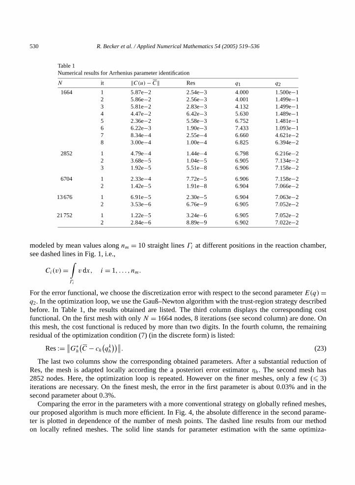
Comparing the error in the parameters with a more conventional strategy on globally refined mour proposed algorithm is much more efficient. In Fig. 4, the absolute difference in the second pter is plotted in dependence of the number of mesh points. The dashed line results from ouron locally refined meshes. The solid line stands for parameter estimation with the same op
R. Becker et al. / Applied Numerical Mathematics 54 (2005) 519–536 531
ly refined
er left to
cessaryrefined
n. Thes.
Fig. 4. Relative error in the second Arrhenius parameter in dependence of the number of mesh points. Solid line: globalmeshes; dashed line: locally refined meshes on the basis of a posteriori error estimation.
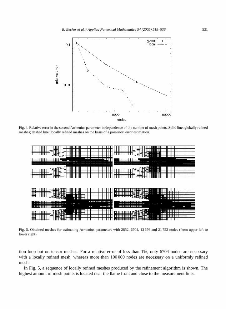
Fig. 5. Obtained meshes for estimating Arrhenius parameters with 2852, 6704, 13 676 and 21 752 nodes (from upplower right).
tion loop but on tensor meshes. For a relative error of less than 1%, only 6704 nodes are newith a locally refined mesh, whereas more than 100 000 nodes are necessary on a uniformlymesh.
In Fig. 5, a sequence of locally refined meshes produced by the refinement algorithm is showhighest amount of mesh points is located near the flame front and close to the measurement line
532 R. Becker et al. / Applied Numerical Mathematics 54 (2005) 519–536
uations
al
educts
.
pro-
pecies,ecties massnn-
6. Identification of diffusion parameters
In this example, we consider a stationary ozone flame modeled by the following system of eqfor velocitiesv, pressurep, temperatureT and mass fractionsyk:
div(ρv) = 0, (ρv · ∇)v + divπ + ∇p = 0,
ρv · ∇T − 1
cp
divQ= −∑i∈S
hifi, ρv · ∇yk + divFk = fk, k ∈ S.
The specific enthalpies are denoted byhi , the heat capacity at constant pressure is denoted bycp. Bothquantities are evaluated by the use of thermodynamic data bases. The setS denotes the set of chemicspecies. The densityρ is given by the perfect gas law in a mixture with partial molecular weightsmi andthe uniform gas constantR:
ρ = p
RT
(∑i∈S
yi
mi
)−1
.
The stress tensorπ is given as usual for compressible flows. The reaction termsfi are modeled byArrhenius laws for reactions with reaction rateskr :
fi = mi
∑r∈R
(ν ′ri − νri)kr
∏s∈S
cνrj
j , kr = ArTβr exp
− Er
RT
.
The setR includes all reactions considered. The stoichiometric coefficients of the products andfor reactionr are denoted byν ′
ri and νri , respectively. The concentrationci of speciesi is given byci = ρyi/mi . The heat fluxQ is given by Fourier’s lawQ = −q0λ∇T , whereλ is the heat conductivityThe species fluxesFk are modeled by a simple Fick law:
Fk = −qkD∗k∇yk. (24)
The scaling parametersqk are the free parameters which have to be calibrated in the optimizationcedure. Following Hirschfelder and Curtiss [16], the diffusion coefficients in the mixtureD∗
k are givenby
D∗k = (1− yk)
(∑l =k
xl
Dbinkl
)−1
,
with binary diffusion coefficientsDbinkl and mole fractionsxl .
6.1. Configuration of an ozone decomposition flame
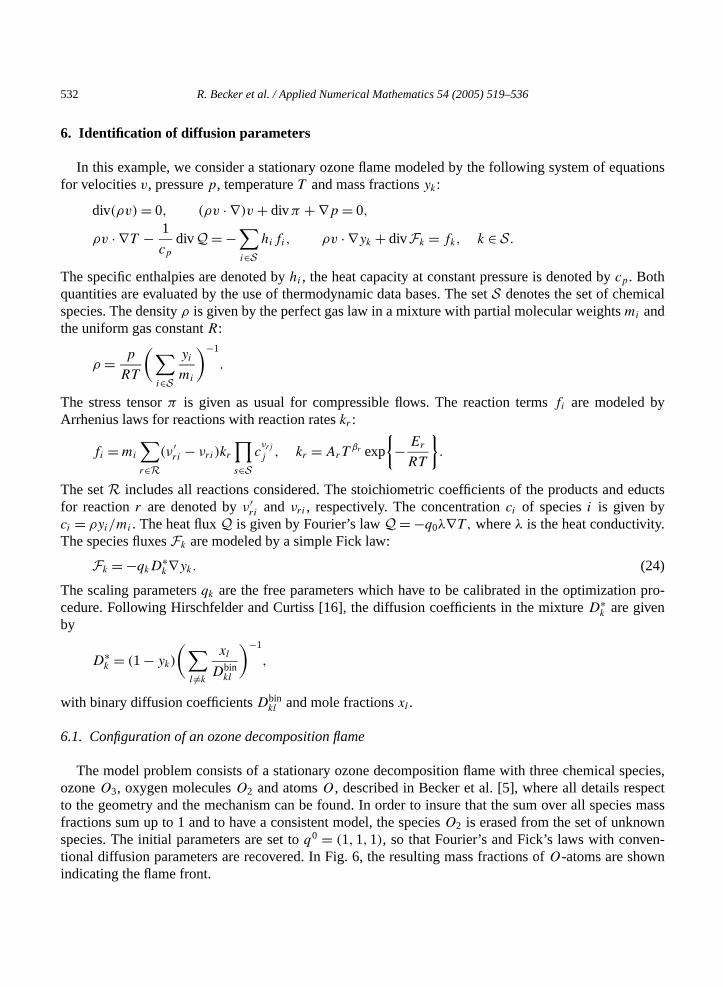
The model problem consists of a stationary ozone decomposition flame with three chemical sozoneO3, oxygen moleculesO2 and atomsO, described in Becker et al. [5], where all details respto the geometry and the mechanism can be found. In order to insure that the sum over all specfractions sum up to 1 and to have a consistent model, the speciesO2 is erased from the set of unknowspecies. The initial parameters are set toq0 = (1,1,1), so that Fourier’s and Fick’s laws with convetional diffusion parameters are recovered. In Fig. 6, the resulting mass fractions ofO-atoms are shownindicating the flame front.
R. Becker et al. / Applied Numerical Mathematics 54 (2005) 519–536 533
fusion
sstheimizedent.spect to
cy
hows
Newtonerefore,e part ofence of
ons for.
Fig. 6. Oxygen atoms for the initial diffusion model (Fick’s law).
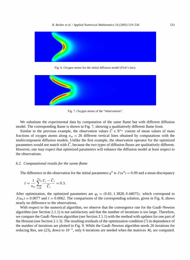
Fig. 7. Oxygen atoms of the “observations”.
We substitute the experimental data by computation of the same flame but with different difmodel. The corresponding flame is shown in Fig. 7, showing a qualitatively different flame front.
Similar to the previous example, the observation valuesC ∈ Rnm consist of mean values of ma
fractions of oxygen atoms alongnm = 26 different vertical lines obtained by computations withmulticomponent diffusion models. Unlike the first example, the observation operator for the optparameters would not match withC, because the two types of diffusion fluxes are qualitatively differHowever, one may expect that optimized parameters will enhance the diffusion model at least rethe observations.
6.2. Computational results for the ozone flame
The difference in the observation for the initial parametersq0 is J (u0) = 0.09 and a mean discrepan
ε = 1
nm
nm∑i=0
Ci − Ci
Ci
= 0.3.
After optimization, the optimized parameters areqh = (0.65,1.3828,0.44075), which correspond toJ (uh) = 0.0077 andε = 0.0062. The comparisons of the corresponding solution, given in Fig. 8, snearly no difference to the observations.
With respect to the numerical algorithm, we observe that the convergence rate for the Gauß–algorithm (see Section 2.1.1) is not satisfactory and that the number of iterations is too large. Thwe compare the Gauß–Newton algorithm (see Section 2.1.1) with the method with updates for onthe Hessian (see Section 2.1.3). The resulting residuals of the optimization condition (7) in dependthe number of iterations are plotted in Fig. 9. While the Gauß–Newton algorithm needs 26 iteratireducing Res, see (23), down to 10−5, only 6 iterations are needed when the matricesM are computed
k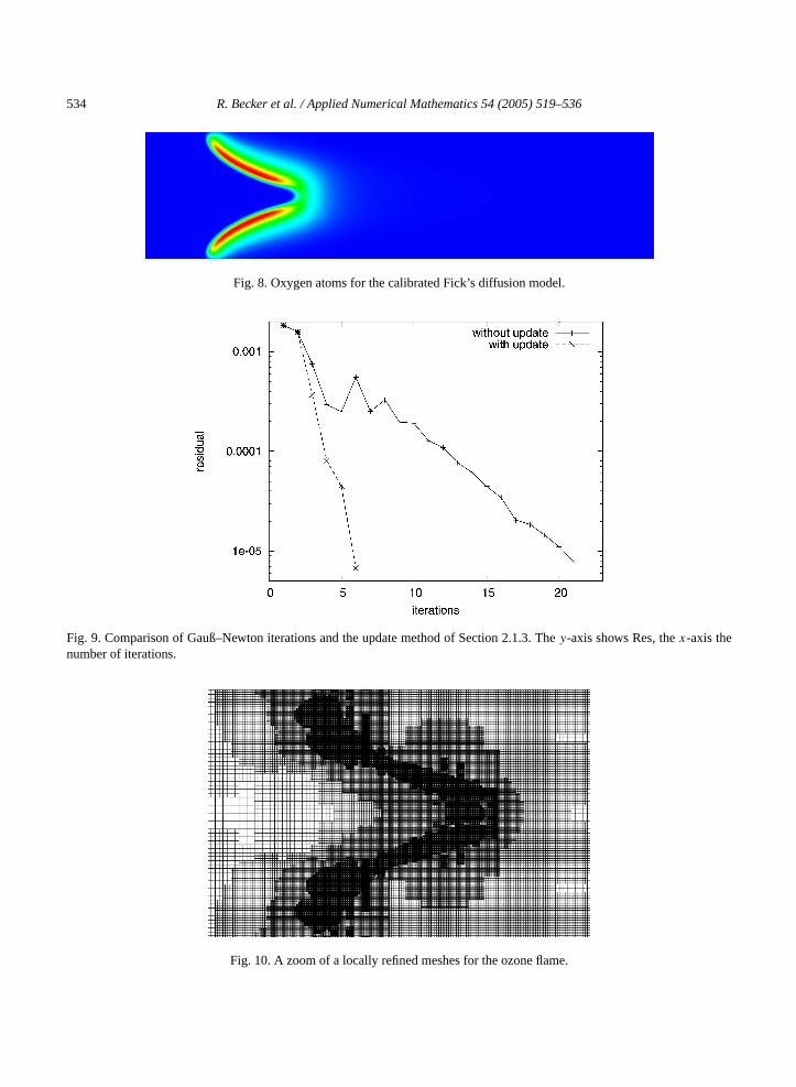
534 R. Becker et al. / Applied Numerical Mathematics 54 (2005) 519–536
Fig. 8. Oxygen atoms for the calibrated Fick’s diffusion model.
Fig. 9. Comparison of Gauß–Newton iterations and the update method of Section 2.1.3. They-axis shows Res, thex-axis thenumber of iterations.
Fig. 10. A zoom of a locally refined meshes for the ozone flame.
R. Becker et al. / Applied Numerical Mathematics 54 (2005) 519–536 535
residual
for this
jections,
xamples,
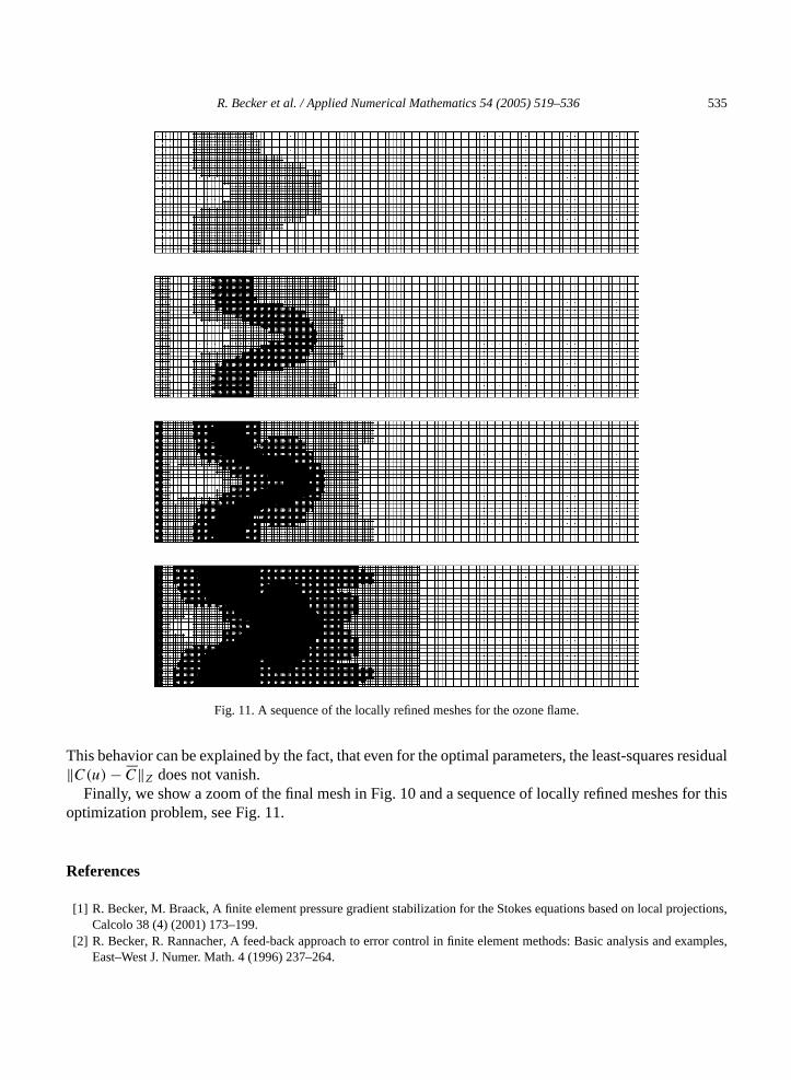
Fig. 11. A sequence of the locally refined meshes for the ozone flame.
This behavior can be explained by the fact, that even for the optimal parameters, the least-squares‖C(u) − C‖Z does not vanish.
Finally, we show a zoom of the final mesh in Fig. 10 and a sequence of locally refined meshesoptimization problem, see Fig. 11.
References
[1] R. Becker, M. Braack, A finite element pressure gradient stabilization for the Stokes equations based on local proCalcolo 38 (4) (2001) 173–199.
[2] R. Becker, R. Rannacher, A feed-back approach to error control in finite element methods: Basic analysis and eEast–West J. Numer. Math. 4 (1996) 237–264.
536 R. Becker et al. / Applied Numerical Mathematics 54 (2005) 519–536
ods, in:
blems,
e finite
1 (2)
–84.
lassics in
1) 348–
001.. Anal.
iversity
Pro-wr.uni-
9.tion sys-blems in
[3] R. Becker, R. Rannacher, An optimal control approach to a posteriori error estimation in finite element methA. Iserles (Ed.), Acta Numerica 2001, Cambridge University Press, Cambridge, 2001, pp. 1–102.
[4] R. Becker, B. Vexler, A posteriori error estimation for finite element discretization of parameter identification proNumer. Math. 96 (3) (2004) 435–459.
[5] R. Becker, M. Braack, R. Rannacher, Numerical simulation of laminar flames at low Mach number with adaptivelements, Combust. Theory Modelling 3 (1999) 503–534.
[6] M. Braack, A. Ern, A posteriori control of modeling errors and discretization errors, Multiscale Model. Simulation(2003) 221–238.
[7] G. Carey, J. Oden, Finite Elements, Computational Aspects, vol. III, Prentice-Hall, Englewood Cliffs, NJ, 1984.[8] P. Ciarlet, Finite Element Methods for Elliptic Problems, North-Holland, Amsterdam, 1978.[9] P. Clément, Approximation by finite element functions using local regularization, RAIRO Anal. Numer. 9 (1975) 77
[10] A.R. Conn, N. Gould, P. Toint, Trust-Region Methods, SIAM, MPS, Philadelphia, PA, 2000.[11] J. Dennis, R. Schnabel, Numerical methods for unconstrained optimization and nonlinear equations equations, C
Applied Mathematics, SIAM.[12] J. Dennis, D. Gay, R. Welsch, An adaptive nonlinear least-squares algorithm, ACM Trans. Math. Software 7 (198
368.[13] J. Dieudonné, Fondation of Modern Analysis, Academic Press, New York, 1960.[14] P. Englezos, N. Kalogerakis, Applied Parameter Estimation for Chemical Engineers, Marcel Dekker, New York, 2[15] J.-L. Guermond, Stabilization of Galerkin approximations of transport equations by subgrid modeling, Modél. Math
Numér. 33 (6) (1999) 1293–1316.[16] J.O. Hirschfelder, C.F. Curtiss, Flame and Explosion Phenomena, Williams and Wilkins, Baltimore, MD, 1949.[17] C. Johnson, Numerical Solution of Partial Differential Equations by the Finite Element Method, Cambridge Un
Press, Cambridge, 1987.[18] T.W. Lohmann, Modelling of reaction kinetics in coal pyrolysis, in: J. Warnatz, F. Behrendt (Eds.),
ceedings of the International Workshop: Modelling of Chemical Reaction Systems, 1996, http://reaflow.iheidelberg.de/~crs96/Program/Contrib/a28lo.htm.
[19] J. Nocedal, S. Wright, Numerical Optimization, Springer Series in Operations Research, Springer, New York, 199[20] M.W. Ziesse, H.G. Bock, J.V. Gallitzendörfer, J.P. Schlöder, Parameter estimation in multispecies transport reac
tems using parallel algorithms, in: J. Gottlieb, P. DuChateaux (Eds.), Parameter Identification and Inverse ProHydrology, Geology and Ecology, Kluwer Academic, Dordrecht, 1996.